114

In this chapter, we show how individual demand curves are “added up” to createthe market demand curve for a good. Market demand curves reflect the actionsof many people and show how these actions are affected by market prices.

This chapter also describes a few ways of measuring market demand. We in-troduce the concept of elasticity and show how we can use it to summarize howthe quantity demanded of a good changes in response to changes in income andprices.

I MARKET DEMAND CURVES

The market demand for a good is the total quantity of the good demanded by allpotential buyers. The market demand curve shows the relationship between thistotal quantity demanded and the market price of the good, when all other thingsthat affect demand are held constant. The market demand curve’s shape and po-sition are determined by the shape of individuals’ demand curves for the productin question. Market demand is nothing more than the combined effect of eco-nomic choices by many consumers.

Construction of the Market Demand CurveFigure 4-1 shows the construction of the market demand curve for good X whenthere are only two buyers. For each price, the point on the market demand curveis found by summing the quantities demanded by each person. For example, at aprice of P*X, individual 1 demands X*1, and individual 2 demands X*2. The totalquantity demanded at the market at P*X is therefore the sum of these twoamounts: X* 5 X*1 1 X*2. Consequently the point X*, P*X is one point on themarket demand curve D. The other points on the curve are plotted in the sameway. The market curve is simply the horizontal sum of each person’s demand

Market Demand and Elasticity

Market demandThe total quantity ofa good or servicedemanded by allpotential buyers.

Market demandcurveThe relationshipbetween the totalquantity demandedof a good or serviceand its price,holding all otherfactors constant.

Market Demand and Elasticity4

1969X_Ch04pp3 1/4/06 11:18 AM Page 114

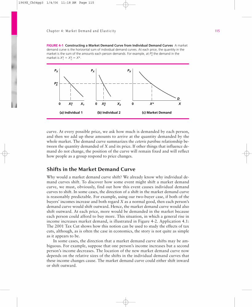
curve. At every possible price, we ask how much is demanded by each person,and then we add up these amounts to arrive at the quantity demanded by thewhole market. The demand curve summarizes the ceteris paribus relationship be-tween the quantity demanded of X and its price. If other things that influence de-mand do not change, the position of the curve will remain fixed and will reflecthow people as a group respond to price changes.

Shifts in the Market Demand CurveWhy would a market demand curve shift? We already know why individual de-mand curves shift. To discover how some event might shift a market demandcurve, we must, obviously, find out how this event causes individual demandcurves to shift. In some cases, the direction of a shift in the market demand curveis reasonably predictable. For example, using our two-buyer case, if both of thebuyers’ incomes increase and both regard X as a normal good, then each person’sdemand curve would shift outward. Hence, the market demand curve would alsoshift outward. At each price, more would be demanded in the market becauseeach person could afford to buy more. This situation, in which a general rise inincome increases market demand, is illustrated in Figure 4-2. Application 4.1:The 2001 Tax Cut shows how this notion can be used to study the effects of taxcuts, although, as is often the case in economics, the story is not quite as simpleas it appears to be.

In some cases, the direction that a market demand curve shifts may be am-biguous. For example, suppose that one person’s income increases but a secondperson’s income decreases. The location of the new market demand curve nowdepends on the relative sizes of the shifts in the individual demand curves thatthese income changes cause. The market demand curve could either shift inwardor shift outward.

C h a p t e r 4 : M a r k e t D e m a n d a n d E l a s t i c i t y 115

FIGURE 4-1 Constructing a Market Demand Curve from Individual Demand Curves A marketdemand curve is the horizontal sum of individual demand curves. At each price, the quantity in themarket is the sum of the amounts each person demands. For example, at P*X the demand in themarket is X*1 1 X*2 5 X*.

(a) Individual 1

PX

P*

X1X*0

(b) Individual 2

PX

X2X*0

(c) Market Demand

PX

X

D

X*0

X

1 2

1969X_Ch04pp3 1/4/06 11:18 AM Page 115

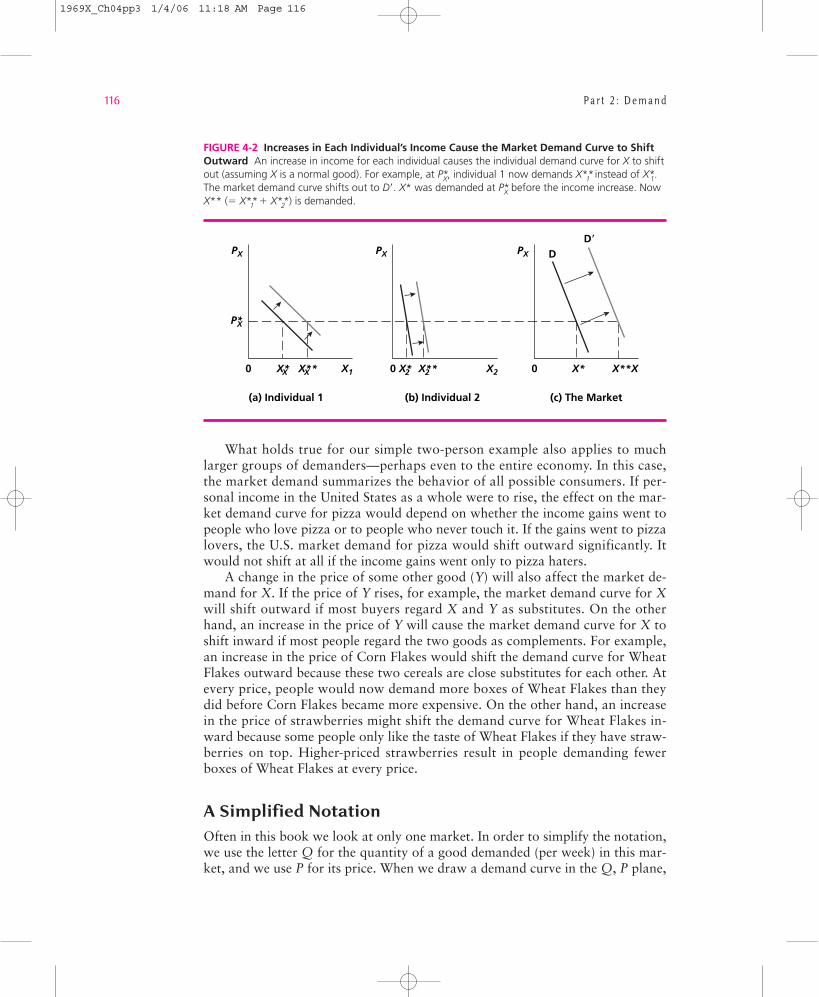
What holds true for our simple two-person example also applies to muchlarger groups of demanders—perhaps even to the entire economy. In this case,the market demand summarizes the behavior of all possible consumers. If per-sonal income in the United States as a whole were to rise, the effect on the mar-ket demand curve for pizza would depend on whether the income gains went topeople who love pizza or to people who never touch it. If the gains went to pizzalovers, the U.S. market demand for pizza would shift outward significantly. Itwould not shift at all if the income gains went only to pizza haters.

A change in the price of some other good (Y) will also affect the market de-mand for X. If the price of Y rises, for example, the market demand curve for Xwill shift outward if most buyers regard X and Y as substitutes. On the otherhand, an increase in the price of Y will cause the market demand curve for X toshift inward if most people regard the two goods as complements. For example,an increase in the price of Corn Flakes would shift the demand curve for WheatFlakes outward because these two cereals are close substitutes for each other. Atevery price, people would now demand more boxes of Wheat Flakes than theydid before Corn Flakes became more expensive. On the other hand, an increasein the price of strawberries might shift the demand curve for Wheat Flakes in-ward because some people only like the taste of Wheat Flakes if they have straw-berries on top. Higher-priced strawberries result in people demanding fewerboxes of Wheat Flakes at every price.

A Simplified NotationOften in this book we look at only one market. In order to simplify the notation,we use the letter Q for the quantity of a good demanded (per week) in this mar-ket, and we use P for its price. When we draw a demand curve in the Q, P plane,

116 P a r t 2 : D e m a n d

FIGURE 4-2 Increases in Each Individual’s Income Cause the Market Demand Curve to ShiftOutward An increase in income for each individual causes the individual demand curve for X to shiftout (assuming X is a normal good). For example, at P*X, individual 1 now demands X**1 instead of X*1.The market demand curve shifts out to D9. X* was demanded at P*X before the income increase. NowX** (5 X**1 1 X**2 ) is demanded.

(a) Individual 1

PX

P*

X1X* X**0

(b) Individual 2

PX

X2X* X**0

(c) The Market

PX

X

DD�

X* X**0

X

X X 2 2

1969X_Ch04pp3 1/4/06 11:18 AM Page 116

In May 2001, the U.S. Congress passed one of thelargest cuts in personal income taxes in history. Thecuts are to be implemented over a 10-year periodand will (over that period) amount to more than$1.6 trillion. As a “down payment” on this sum,the law provided that most U.S. taxpayers receivean immediate check for $300 (or $600 for a mar-ried couple), and these checks rolled out of theTreasury at the rate of 9 million per week during thesummer of 2001. Many politicians argued that sucha large tax reduction would have an important ef-fect on fighting the recession that was then begin-ning, by boosting the demand for virtually everygood. But such a prediction ignored both economictheory and the realities of the bizarre U.S. tax sys-tem. Ultimately, the tax cut seems to have had vir-tually no immediate impact on consumer spending.

The Permanent Income HypothesisOur discussion of demand theory showed thatchanges in people’s incomes do indeed shift de-mand curves outward. But we have been a bitcareless in defining exactly what income is. MiltonFriedman made one of the most important dis-coveries that clarify this question in the 1950s. Heargued that spending decisions are based on a per-son’s long-term view of his or her economic cir-cumstances.1 Short-term increases or decreases inincome have little effect on spending patterns.Friedman’s view that spending decisions are basedon a person’s “permanent” income is now widelyaccepted by economists.

Tax Cuts and Permanent IncomeAccording to Friedman’s theory, a tax reduction willaffect a person’s spending only to the extent that itaffects his or her permanent income. This insightsuggests that the 2001 tax act had little impact fortwo reasons. First, consider the $300 checks. Thesecame to people “out of the blue,” and everyoneknew that such largess would not continue. Thechecks were too small to stimulate spending on anymajor goods, so they were largely saved. In this,they were exhibiting exactly the same sort of non-response that they had shown in many previousepisodes, including temporary tax increases in thelate 1960s and temporary reductions in the 1970s.

Now consider the effect of the overall tax act, aplan that was intended to be implemented over a

10-year period. Because of wrangling in Congress,the actual schedule of tax cuts is “back-loaded.”That is, most of the cuts do not begin until 2006,and the largest cuts are reserved until 2009–2010.Such distant tax cuts probably have little immediateimpact on people’s perceptions of their economicsituations. In purely dollar terms, the present valueof such distant tax savings is much smaller thantheir actual stated amounts.2 Perhaps more impor-tant, taxpayers may have had little faith that taxcuts projected for many years in the future will ac-tually occur. That is, many of the tax reductionspromised under the 2001 act were simply not“credible.”

Complexities in the Income TaxAnother set of reasons that led to the sluggishresponse to the 2001 tax cuts relates to the com-plexities in the U.S. income tax itself. First, all ofthe rate changes in the bill were subject to “sun-set” provisions—in 2011, tax rates are supposedto return to 2001 levels. In effect, the entire taxbill is a temporary one. What happens after 2011is anyone’s guess. Second, the bill did not dealwith the alternative minimum tax (AMT)—a pro-vision of the U.S. income tax originally intendedto catch fat cats who pay little taxes, but one thathas increasingly affected middle-income taxpay-ers. Under this arcane provision, much of the ef-fect of the tax reductions promised under the2001 act will be neutralized by increased taxescollected under the AMT. Finally, many of the taxreductions in the 2001 bill came about throughspecial credits for all sorts of items such as col-lege tuitions and energy conservation. How theseactually affect the purchasing power of the aver-age citizen obviously depends on whether theywish to spend their incomes on the especially fa-vored items. Certainly not everyone’s budget waspositively affected.

To Think About1. If a person makes economic decisions based on

his or her permanent income, how much mightbe spent currently out of an unexpected $300check from the government?

2. How might various people differ in the ways inwhich they respond to getting a tax rebatecheck from the government?

C h a p t e r 4 : M a r k e t D e m a n d a n d E l a s t i c i t y 117

Application 4.1 The 2001 Tax Cut

1 Milton Friedman, A Theory of the Consumption Function(Princeton, NJ: Princeton University Press, 1957). Recentamendments to Friedman’s theory stress the “life-cycle”nature of income and spending decisions—that is, peopleare assumed to plan their spending over their entire lives.

2 The present value of a sum payable in the future is lessthan the actual amount because of forgone interest. Fora discussion of this concept, see Chapter 16 and itsAppendix.

1969X_Ch04pp3 1/4/06 11:18 AM Page 117

we assume that all other factors affecting demand are held constant. That is, in-come, the price of other goods, and preferences are assumed not to change. If oneof these factors happened to change, the demand curve would shift to a new lo-cation. As was the case for individual demand curves, the term “change in quan-tity demanded” is used for a movement along a given market demand curve (inresponse to a price change), and the term “change in demand” is used for a shiftin the entire curve.

I ELASTICITY

Economists frequently need to show how changes in one variable affect someother variable. They ask, for example, how much does a change in the price of

electricity affect the quantity of it demanded,or how does a change in income affect totalspending on automobiles? One problem insummarizing these kinds of effects is that goodsare measured in different ways. For example,steak is typically sold per pound, whereas or-anges are generally sold per dozen. A $0.10 perpound rise in the price of steak might cause na-tional consumption of steak to fall by 100,000pounds per week, and a $0.10 per dozen rise inthe price of oranges might cause national or-ange purchases to fall by 50,000 dozen perweek. But there is no good way to compare thechange in steak sales to the change in orangesales. When two goods are measured in differ-ent units, we cannot make a simple comparison

between the demand for them to determine which demand is more responsive tochanges in its price.

Economists solve this measurement problem in a two-step process. First, theypractically always talk about changes in percentage terms. Rather than sayingthat the price of oranges, say, rose by $0.10 per dozen, from $2.00 to $2.10, theywould instead report that orange prices rose by 5 percent. Similarly, a fall inorange prices of $0.10 per dozen would be regarded as a change of minuspercent.

Percentage changes can, of course, also be calculated for quantities. If na-tional orange purchases fell from 500,000 dozen per week to 450,000, we wouldsay that such purchases fell by 10 percent (that is, they changed by minus 10 per-cent). An increase in steak sales from 2 million pounds per week to 2.1 millionpounds per week would be regarded as a 5 percent increase.

The advantage of always talking in terms of percentage changes is that wedon’t have to worry very much about the actual units of measurement beingused. If orange prices fall by 5 percent, this has the same meaning regardlessof whether we are paying for them in dollars, yen, marks, or pesos. Similarly, an

118 P a r t 2 : D e m a n d

A shift outward in a demand curve can be de-scribed either by the extent of its shift in thehorizontal direction or by its shift in the verticaldirection. How would the following shifts beshown graphically?

1. News that nutmeg cures the common coldcauses people to demand 2 million pounds morenutmeg at each price.

2. News that nutmeg cures the common coldcauses people to be willing to pay $1 more perpound of nutmeg for each possible quantity.

M I C R O Q U I Z 4 . 1

1969X_Ch04pp3 1/4/06 11:18 AM Page 118

increase in the quantity of oranges sold of 10 percent means the same thing re-gardless of whether we measure orange sales in dozens, crates, or boxcars full.

The second step in solving the measurement problem is to link percentagechanges when they have a cause/effect relationship. For example, if a 5 percentfall in the price of oranges typically results in a 10 percent increase in quantitybought (when everything else is held constant), we could link these two facts andsay that each percent fall in the price of oranges leads to an increase in sales ofabout 2 percent. That is, we would say that the “elasticity” of orange sales withrespect to price changes is about 2 (actually, as we discuss in the next section,minus 2 because price and quantity move in opposite directions). This approachis quite general and is used throughout economics. Specifically, if economists be-lieve that variable A affects variable B, they define the elasticity of B with respectto A as the percent change in B for each percentage point change in A. The num-ber that results from this calculation is unit-free. It can readily be comparedacross different goods, between different countries, or over time.

I PRICE ELASTICITY OF DEMAND

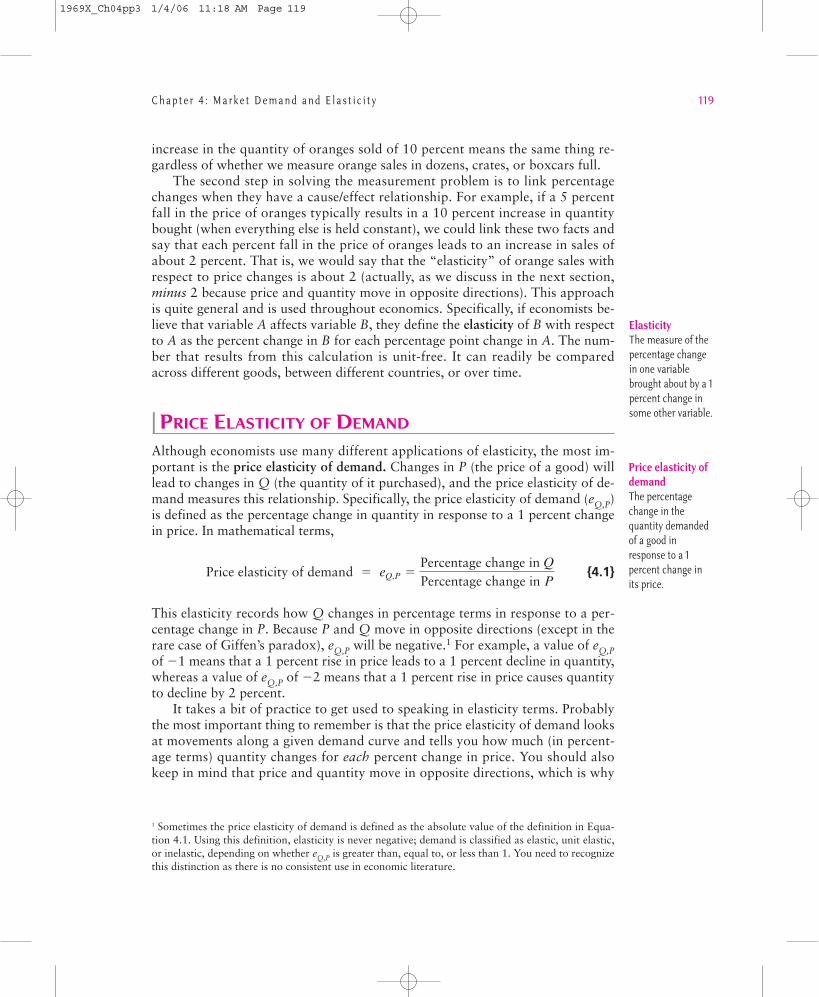
Although economists use many different applications of elasticity, the most im-portant is the price elasticity of demand. Changes in P (the price of a good) willlead to changes in Q (the quantity of it purchased), and the price elasticity of de-mand measures this relationship. Specifically, the price elasticity of demand (eQ,P)is defined as the percentage change in quantity in response to a 1 percent changein price. In mathematical terms,

{4.1}

This elasticity records how Q changes in percentage terms in response to a per-centage change in P. Because P and Q move in opposite directions (except in therare case of Giffen’s paradox), eQ,P will be negative.1 For example, a value of eQ,Pof 21 means that a 1 percent rise in price leads to a 1 percent decline in quantity,whereas a value of eQ,P of 22 means that a 1 percent rise in price causes quantityto decline by 2 percent.

It takes a bit of practice to get used to speaking in elasticity terms. Probablythe most important thing to remember is that the price elasticity of demand looksat movements along a given demand curve and tells you how much (in percent-age terms) quantity changes for each percent change in price. You should alsokeep in mind that price and quantity move in opposite directions, which is why

Price elasticity of demand 5 eQ,P 5Percentage change in QPercentage change in P

C h a p t e r 4 : M a r k e t D e m a n d a n d E l a s t i c i t y 119

ElasticityThe measure of thepercentage changein one variablebrought about by a 1percent change insome other variable.

Price elasticity ofdemandThe percentagechange in thequantity demandedof a good inresponse to a 1percent change inits price.

1 Sometimes the price elasticity of demand is defined as the absolute value of the definition in Equa-tion 4.1. Using this definition, elasticity is never negative; demand is classified as elastic, unit elastic,or inelastic, depending on whether eQ,P is greater than, equal to, or less than 1. You need to recognizethis distinction as there is no consistent use in economic literature.

1969X_Ch04pp3 1/4/06 11:18 AM Page 119

the price elasticity of demand is negative. For example, suppose that studies haveshown that the price elasticity of demand for gasoline is 22. That means thatevery percent rise in price will cause a movement along the gasoline demandcurve reducing quantity demanded by 2 percent. So, if gasoline prices rise by, say,6 percent, we know that (if nothing else changes) quantity will fall by 12 percent( 5 6 3 [22] ). Similarly, if the gasoline price were to fall by 4 percent, this priceelasticity could be used to predict that gasoline purchases would rise by 8 per-cent ( 5 [24] 3 [22] ). Sometimes price elasticities take on decimal values, butthis should pose no problem. If, for example, the price elasticity of demand foraspirin were found to be 20.3, this would mean that each percentage point risein aspirin prices would cause quantity demanded to fall by 0.3 percent (that is,by three-tenths of 1 percent). So, if aspirin prices rose by 15 percent (and every-thing else that affects aspirin demand stayed fixed), we could predict that thequantity of aspirin demanded would fall by 4.5 percent (5 15 3 [20.3] ).

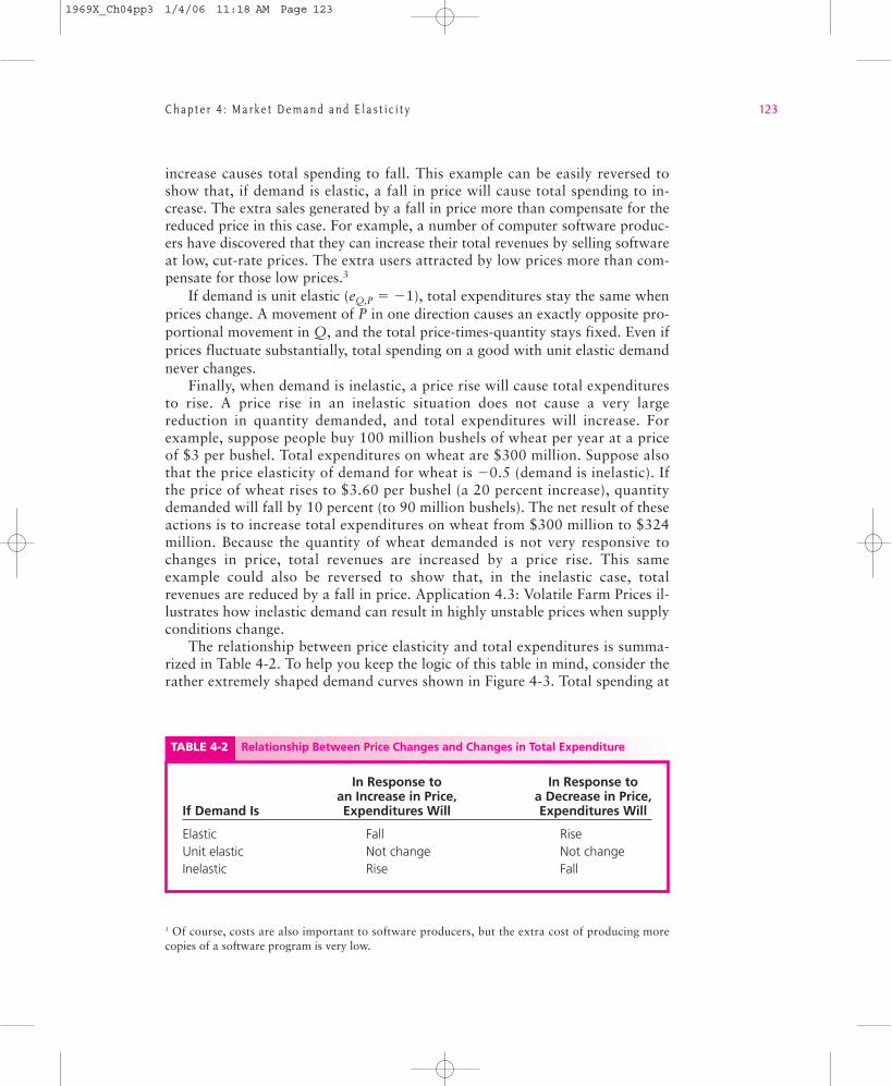
Values of the Price Elasticity of DemandA distinction is usually made among values of eQ,P that are less than, equal to, orgreater than 21. Table 4-1 lists the terms used for each value. For an elasticcurve (eQ,P is less than 21),2 a price increase causes a more than proportionalquantity decrease. If eQ,P 5 23, for example, each 1 percent rise in price causesquantity to fall by 3 percent. For a unit elastic curve (eQ,P is equal to 21), a priceincrease causes a decrease in quantity of the same proportion. For an inelasticcurve (eQ,P is greater than 21), price increases proportionally more than quan-tity decreases. If eQ,P 5 21⁄2, a 1 percent rise in price causes quantity to fall byonly 1⁄2 of 1 percent. In general then, if a demand curve is elastic, changes in pricealong the curve affect quantity significantly; if the curve is inelastic, price has lit-tle effect on quantity demanded.

Price Elasticity and theSubstitution EffectThe discussion of income and substi-tution effects in Chapter 3 provides abasis for judging what the size of theprice elasticity for particular goodsmight be. Goods with many close sub-stitutes (brands of breakfast cereal,small cars, brands of electronic calcu-

120 P a r t 2 : D e m a n d

2 Remember, numbers like 23 are less than 21, whereas 21⁄2 is greater than 21. Because we are ac-customed to thinking only of positive numbers, statements about the size of price elasticities cansometimes be confusing.

TABLE 4-1 Terminology for the Ranges of EQ,P

Value of eQ,P at a Point Terminology for Curveon Demand Curve at This Point

eQ,P , 21 ElasticeQ,P 5 2 1 Unit elasticeQ,P . 2 1 Inelastic

1969X_Ch04pp3 1/4/06 11:18 AM Page 120

lators, and so on) are subject to large substitution effects from a price change.For these kinds of goods, we can presume that demand will be elastic (eQ,P ,

21). On the other hand, goods with few close substitutes (water, insulin, andsalt, for example) have small substitution effects when their prices change. De-mand for such goods will probably be inelastic with respect to price changes (eQ,P. 21; that is, eQ,P is between 0 and 21). Of course, as we mentioned previously,price changes also create income effects on the quantity demanded of a good,which we must consider to completely assess the likely size of overall price elas-ticities. Still, because the price changes for most goods have only a small effecton people’s real incomes, the existence (or nonexistence) of substitutes is proba-bly the principal determinant of price elasticity.

Price Elasticity and TimeMaking substitutions in consumption choices may take time. To change fromone brand of cereal to another may only take a week (to finish eating the firstbox), but to change from heating your house with oil to heating it with electric-ity may take years because a new heating system must be installed. We alreadyhave seen in Application 3.4: SUVs and Gasoline Prices that trends in gasolineprices may have little short-term impact because people already own their carsand have relatively fixed travel needs. Over a longer term, however, there is clearevidence that people will change the kinds of cars they drive in response tochanging real gasoline prices. In general then, it might be expected that substitu-tion effects and the related price elasticities would be larger the longer the timeperiod that people have to change their behavior. In some situations it is impor-tant to make a distinction between short-term and long-term price elasticities ofdemand, because the long-term concept may show much greater responses toprice change. In Application 4.2: Brand Loyalty, we look at a few cases wherethis distinction can be important.

Price Elasticity and Total ExpendituresThe price elasticity of demand is useful for studying how total expenditures on agood change in response to a price change. Total expenditures on a good arefound by multiplying the good’s price (P) times the quantity purchased (Q). Ifdemand is elastic, a price increase will cause total expenditures to fall. Whendemand is elastic, a given percentage increase in price is more than counterbal-anced in its effect on total spending by the resulting large decrease in quantitydemanded. For example, suppose people are currently buying 1 million automo-biles at $10,000 each. Total expenditures on automobiles amount to $10 billion.Suppose also that the price elasticity of demand for automobiles is 22. Now, ifthe price increases to $11,000 (a 10 percent increase), the quantity purchasedwould fall to 800,000 cars (a 20 percent fall). Total expenditures on cars are now$8.8 billion ($11,000 times 800,000). Because demand is elastic, the price

C h a p t e r 4 : M a r k e t D e m a n d a n d E l a s t i c i t y 121

1969X_Ch04pp3 1/4/06 11:18 AM Page 121

One reason that substitution effects are larger overlonger periods than over shorter ones is that peopledevelop spending habits that do not change easily.For example, when faced with a variety of brandsconsisting of the same basic product, you may de-velop loyalty to a particular brand, purchasing it ona regular basis. This behavior makes sense becauseyou don’t need to reevaluate products continually.Thus, your decision-making costs are reduced.Brand loyalty also reduces the likelihood of brandsubstitutions, even when there are short-term pricedifferentials. Over the long term, however, price dif-ferences can tempt buyers into trying new brandsand thereby switch their loyalties.

AutomobilesThe competition between American and Japaneseautomakers provides a good example of changingloyalties. Prior to the 1980s, Americans exhibitedconsiderable loyalty to U.S. automobiles. Repeatpurchases of the same brand were a common pat-tern. In the early 1970s, Japanese automobilesbegan making inroads into the American market ona price basis. The lower prices of Japanese carseventually convinced Americans to buy them. Satis-fied with their experiences, by the 1980s manyAmericans developed loyalty to Japanese brands.This loyalty was encouraged, in part, by large differ-ences in quality between Japanese and U.S. cars,which became especially large in the mid-1980s.Although U.S. automakers have worked hard toclose some of the quality gap, lingering loyalty toJapanese autos has made it difficult to regain mar-ket share. By one estimate, U.S. cars would have tosell for approximately $1,600 less than their Japan-ese counterparts in order to encourage buyers ofJapanese cars to switch.1

Licensing of Brand NamesThe advantages of brand loyalty have not been loston innovative marketers. Famous trademarks suchas Coca-Cola, Harley-Davidson, or Disney’s MickeyMouse have been applied to products rather differ-ent from the originals. For example, Coca-Cola fora period licensed its famous name and symbol tomakers of sweatshirts and blue jeans, in the hopethat this would differentiate the products from theirgeneric competitors. Similarly, Mickey Mouse is oneof the most popular trademarks in Japan, appear-ing on products both conventional (watches and

lunchboxes) and unconventional (fashionable hand-bags and neckties).

The economics behind these moves arestraight-forward. Prior to licensing, products arevirtually perfect substitutes and consumers shiftreadily among various makers. Licensing createssomewhat lower price responsiveness for thebranded product, so producers can charge more forit without losing all their sales. The large fees paidto Coca-Cola, Disney, Michael Jordan, or majorleague baseball provide strong evidence of thestrategy’s profitability.

Overcoming Brand LoyaltyA useful way to think about brand loyalty is thatpeople incur “switching costs” when they decide todepart from a familiar brand. Producers of a newproduct must overcome those costs if they are to besuccessful. Temporary price reductions are one wayin which switching costs might be overcome. Heavyadvertising of a new product offers another routeto this end. In general firms would be expected tochoose the most cost-effective approach. For exam-ple, in a study of brand loyalty to breakfast cerealsM. Shum2 used scanner data to look at repeat pur-chases of a number of national brands such asCheerios or Rice Krispies. He found that an increasein a new brands advertising budget of 25 percentreduced the costs associated with switching from amajor brand by about $0.68—a figure that repre-sents about a 15 percent reduction. The authorshowed that obtaining a similar reduction in switch-ing costs through temporary price reductions wouldbe considerably more costly to the producers of anew brand.

To Think About1. Does the speed with which price differences

erode brand loyalties depend on the frequencywith which products are bought? Why mightdifferences between short-term and long-termprice elasticities be much greater for brands ofautomobiles than for brands of toothpaste?

2. Why do people buy licensed products whenthey could probably buy generic brands at muchlower prices? Does the observation that peoplepay 50 percent more for Nike golf shoes en-dorsed by Tiger Woods than for identical no-name competitors violate the assumptions ofutility maximization?

Application 4.2 Brand Loyalty

1 F. Mannering and C. Winston, “Brand Loyalty and theDecline of American Automobile Firms,” Brookings Paperson Economic Activity, Microeconomics (1991): 67–113.

2 M. Shum, “Does Advertising Overcome Brand Loyalty?Evidence from the Breakfast Cereals Market,” Journal ofEconomics and Management Strategy, Summer, 2004:241–272.

122 P a r t 2 : D e m a n d

1969X_Ch04pp3 1/24/06 2:39 PM Page 122

C h a p t e r 4 : M a r k e t D e m a n d a n d E l a s t i c i t y 123

increase causes total spending to fall. This example can be easily reversed toshow that, if demand is elastic, a fall in price will cause total spending to in-crease. The extra sales generated by a fall in price more than compensate for thereduced price in this case. For example, a number of computer software produc-ers have discovered that they can increase their total revenues by selling softwareat low, cut-rate prices. The extra users attracted by low prices more than com-pensate for those low prices.3

If demand is unit elastic (eQ,P 5 21), total expenditures stay the same whenprices change. A movement of P in one direction causes an exactly opposite pro-portional movement in Q, and the total price-times-quantity stays fixed. Even ifprices fluctuate substantially, total spending on a good with unit elastic demandnever changes.

Finally, when demand is inelastic, a price rise will cause total expendituresto rise. A price rise in an inelastic situation does not cause a very largereduction in quantity demanded, and total expenditures will increase. Forexample, suppose people buy 100 million bushels of wheat per year at a priceof $3 per bushel. Total expenditures on wheat are $300 million. Suppose alsothat the price elasticity of demand for wheat is 20.5 (demand is inelastic). Ifthe price of wheat rises to $3.60 per bushel (a 20 percent increase), quantitydemanded will fall by 10 percent (to 90 million bushels). The net result of theseactions is to increase total expenditures on wheat from $300 million to $324million. Because the quantity of wheat demanded is not very responsive tochanges in price, total revenues are increased by a price rise. This sameexample could also be reversed to show that, in the inelastic case, totalrevenues are reduced by a fall in price. Application 4.3: Volatile Farm Prices il-lustrates how inelastic demand can result in highly unstable prices when supplyconditions change.

The relationship between price elasticity and total expenditures is summa-rized in Table 4-2. To help you keep the logic of this table in mind, consider therather extremely shaped demand curves shown in Figure 4-3. Total spending at

3 Of course, costs are also important to software producers, but the extra cost of producing morecopies of a software program is very low.

TABLE 4-2 Relationship Between Price Changes and Changes in Total Expenditure

In Response to In Response toan Increase in Price, a Decrease in Price,

If Demand Is Expenditures Will Expenditures Will

Elastic Fall RiseUnit elastic Not change Not changeInelastic Rise Fall

1969X_Ch04pp3 1/4/06 11:18 AM Page 123

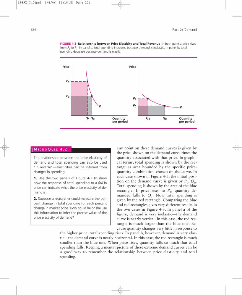
any point on these demand curves is given bythe price shown on the demand curve times thequantity associated with that price. In graphi-cal terms, total spending is shown by the rec-tangular area bounded by the specific price-quantity combination chosen on the curve. Ineach case shown in Figure 4-3, the initial posi-tion on the demand curve is given by P0, Q0.Total spending is shown by the area of the bluerectangle. If price rises to P1, quantity de-manded falls to Q1. Now total spending isgiven by the red rectangle. Comparing the blueand red rectangles gives very different results inthe two cases in Figure 4-3. In panel a of thefigure, demand is very inelastic—the demandcurve is nearly vertical. In this case, the red rec-tangle is much larger than the blue one. Be-cause quantity changes very little in response to

the higher price, total spending rises. In panel b, however, demand is very elas-tic—the demand curve is nearly horizontal. In this case, the red rectangle is muchsmaller than the blue one. When price rises, quantity falls so much that totalspending falls. Keeping a mental picture of these extreme demand curves can bea good way to remember the relationship between price elasticity and totalspending.

124 P a r t 2 : D e m a n d

FIGURE 4-3 Relationship between Price Elasticity and Total Revenue In both panels, price risesfrom P0 to P1. In panel a, total spending increases because demand is inelastic. In panel b, totalspending decrease because demand is elastic.

Quantityper period

P0

P1

Price

Q1 Q0 Quantityper period

P0

P1

D D

Price

Q1 Q0

The relationship between the price elasticity ofdemand and total spending can also be used “in reverse”—elasticities can be inferred fromchanges in spending.

1. Use the two panels of Figure 4-3 to showhow the response of total spending to a fall inprice can indicate what the price elasticity of de-mand is.

2. Suppose a researcher could measure the per-cent change in total spending for each percentchange in market price. How could he or she usethis information to infer the precise value of theprice elasticity of demand?

M I C R O Q U I Z 4 . 2

1969X_Ch04pp3 1/4/06 11:18 AM Page 124

C h a p t e r 4 : M a r k e t D e m a n d a n d E l a s t i c i t y 125

The demand for agricultural products is relativelyprice-inelastic. That is especially true for basic cropssuch as wheat, corn, or soybeans. An important im-plication of this inelasticity is that even modestchanges in supply, often brought about by weatherpatterns, can have large effects on the prices ofthese crops. This volatility in crop prices has been afeature of farming throughout all of history.

The Paradox of AgricultureRecognition of the fundamental economics of farmcrops yields paradoxical insights about the influenceof the weather on farmers’ well-being. “Good”weather can produce bountiful crops and abysmallylow prices, whereas “bad” weather (in moderation)can result in attractively high prices. For example,relatively modest supply disruptions in the U.S.grain belt during the early 1970s caused an explo-sion in farm prices. Farmers’ incomes increasedmore than 40 percent over a short, two-year pe-riod. These incomes quickly fell back again whenmore normal weather patterns returned.

This paradoxical situation also results in mis-leading news coverage of localized droughts. Tele-vision news reporters will usually cover droughtsby showing the viewer a shriveled ear of corn, leav-ing the impression that all farmers are being dev-astated. That is undoubtedly true for the farmerwhose parched field is being shown (though he orshe may also have irrigated fields next door). Butthe larger story of local droughts is that the price in-creases they bring benefit most farmers outside theimmediate area—a story that is seldom told.

Volatile Prices and GovernmentProgramsEver since the New Deal of the 1930s, the volatil-ity of U.S. crop prices was moderated through avariety of federal price-support schemes. Theseschemes operated in two ways. First, through vari-ous acreage restrictions, the laws constrained theextent to which farmers could increase their planti-ngs. In many cases, farmers were paid to keep theirland fallow. A second way in which prices weresupported was through direct purchases of crops bythe government. By manipulating purchases andsales from grain reserves, the government was ableto moderate any severe swings in price that mayhave otherwise occurred. All of that seemed tohave ended in 1996 with the passage of the FederalAgricultural Improvement and Reform (FAIR) Act.That act sharply reduced government interventionin farm markets.

Initially, farm prices held up quite well followingthe passage of the FAIR Act. Throughout 1996,they remained significantly above their levels of theearly 1990s. But the increased plantings encour-aged by the act in combination with downturns insome Asian economies caused a decline in cropprices of nearly 20 percent between 1997 and2000. Though prices staged a bit of a rebound inearly 2001, by the end of the year they had againfallen back. Faced with elections in November2002, this created considerable pressure on politi-cians to do something more for farmers. Such pres-sures culminated in the passage of a 10-year, $83billion farm subsidy bill in May of 2002. That billlargely reversed many of the provisions of the FAIRAct. Still, payments to farmers were relatively mod-est in 2004, mainly because farm prices werebuoyed by less-than-bumper crops.

By 2005, however, volatility had returned tocrop prices. Prices fell rather sharply early in theyear, mainly as a result of abundant late winter andspring harvests. Net farm income dipped dramati-cally during this period, falling by about 40 percentas of mid-year. Direct payments from the govern-ment to farmers increased as a result with suchpayments reaching all-time highs. Such paymentsamounted to more than one-third of total netfarm income during the first half of 2005. But noth-ing stays constant in agriculture for very long. Asummer drought in the Midwest and damagecaused by hurricane Katrina in the South causeda sharp upward movement in crop prices after mid-year. Gross receipts by farmers rose, approachingthe levels of 2004. Whether this recent prosperitywill persist is anyone’s guess. The basic price inelas-ticity of demand for most farm products ensuresthat even modest variations in supply will continueto have major consequences for price.

To Think About1. The volatility of farm prices is both good and

bad news for farmers. Since periods of lowprices are often followed by periods of highprices, the long-term welfare of farmers is hardto determine. Would farmers be better off iftheir prices had smaller fluctuations around thesame trend levels?

2. How should fluctuations in foreign demand forU.S. crops be included in a supply-demandmodel? Do such fluctuations make crop priceseven more volatile?

Application 4.3 Volatile Farm Prices

1969X_Ch04pp3 1/4/06 11:18 AM Page 125

126 P a r t 2 : D e m a n d

I DEMAND CURVES AND PRICE ELASTICITY

The relationship between a particular demand curve and the price elasticity it ex-hibits is relatively complicated. Although it is common to talk about the priceelasticity of demand for a good, this usage conveys the false impression that priceelasticity necessarily has the same value at every point on a market demandcurve. A more accurate way of speaking is to say that “at current prices, the priceelasticity of demand is . . .” and, thereby, leave open the possibility that the elas-ticity may take on some other value at a different point on the demand curve. Insome cases, this distinction may be unimportant because the price elasticity ofdemand has the same value over a relatively broad range of a demand curve. Inother cases, the distinction may be important, especially when large movementsalong a demand curve are being considered.

Linear Demand Curves and Price ElasticityProbably the most important illustration of this warning about elasticities occursin the case of a linear (straight-line) demand curve. As one moves along such ademand curve, the price elasticity of demand is always changing value. At highprice levels, demand is elastic; that is, a fall in price increases quantity purchasedmore than proportionally. At low prices, on the other hand, demand is inelastic;a further decline in price has relatively little proportional effect on quantity.

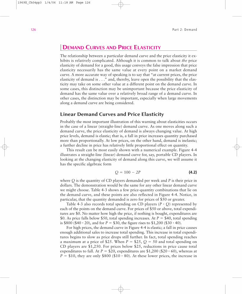
This result can be most easily shown with a numerical example. Figure 4-4illustrates a straight-line (linear) demand curve for, say, portable CD players. Inlooking at the changing elasticity of demand along this curve, we will assume ithas the specific algebraic form

Q 5 100 2 2P {4.2}

where Q is the quantity of CD players demanded per week and P is their price indollars. The demonstration would be the same for any other linear demand curvewe might choose. Table 4-3 shows a few price-quantity combinations that lie onthe demand curve, and these points are also reflected in Figure 4-4. Notice, inparticular, that the quantity demanded is zero for prices of $50 or greater.

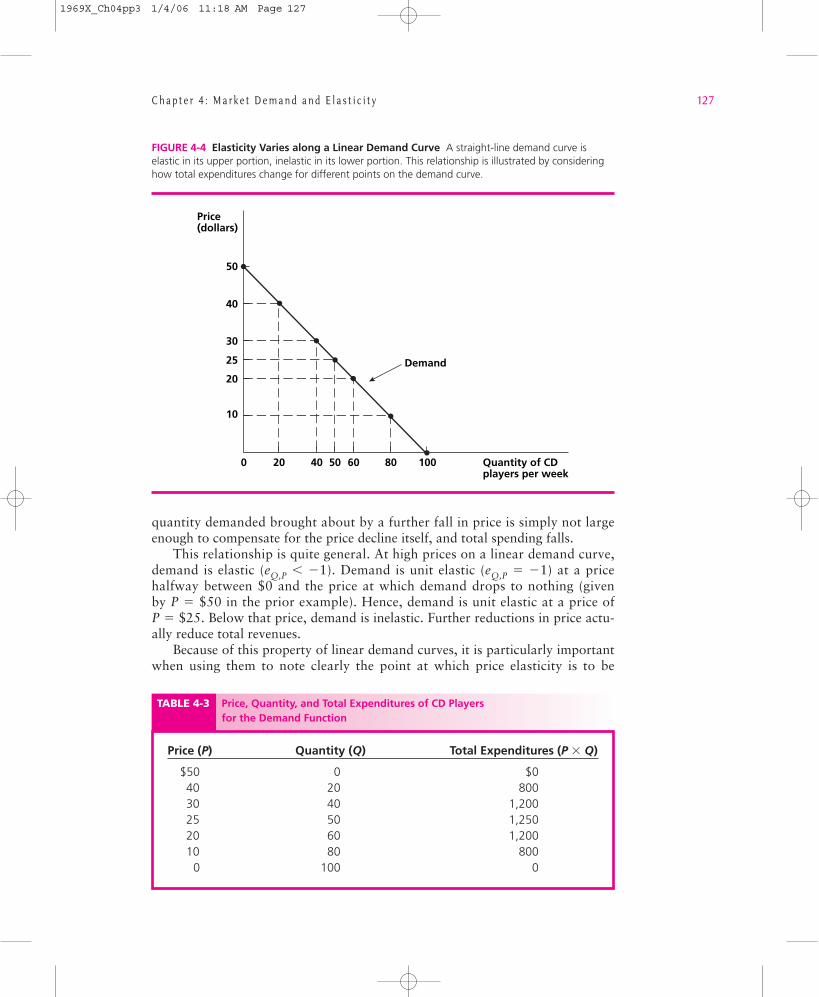
Table 4-3 also records total spending on CD players (P ? Q) represented byeach of the points on the demand curve. For prices of $50 or above, total expendi-tures are $0. No matter how high the price, if nothing is bought, expenditures are$0. As price falls below $50, total spending increases. At P 5 $40, total spendingis $800 ($40 ? 20), and for P 5 $30, the figure rises to $1,200 ($30 ? 40).

For high prices, the demand curve in Figure 4-4 is elastic; a fall in price causesenough additional sales to increase total spending. This increase in total expendi-tures begins to slow as price drops still further. In fact, total spending reachesa maximum at a price of $25. When P 5 $25, Q 5 50 and total spending onCD players are $1,250. For prices below $25, reductions in price cause totalexpenditures to fall. At P 5 $20, expenditures are $1,200 ($20 ? 60), whereas atP 5 $10, they are only $800 ($10 ? 80). At these lower prices, the increase in

1969X_Ch04pp3 1/4/06 11:18 AM Page 126

C h a p t e r 4 : M a r k e t D e m a n d a n d E l a s t i c i t y 127

FIGURE 4-4 Elasticity Varies along a Linear Demand Curve A straight-line demand curve iselastic in its upper portion, inelastic in its lower portion. This relationship is illustrated by consideringhow total expenditures change for different points on the demand curve.

quantity demanded brought about by a further fall in price is simply not largeenough to compensate for the price decline itself, and total spending falls.

This relationship is quite general. At high prices on a linear demand curve,demand is elastic (eQ,P , 21). Demand is unit elastic (eQ,P 5 21) at a pricehalfway between $0 and the price at which demand drops to nothing (givenby P 5 $50 in the prior example). Hence, demand is unit elastic at a price ofP 5 $25. Below that price, demand is inelastic. Further reductions in price actu-ally reduce total revenues.

Because of this property of linear demand curves, it is particularly importantwhen using them to note clearly the point at which price elasticity is to be

TABLE 4-3 Price, Quantity, and Total Expenditures of CD Players for the Demand Function

Price (P) Quantity (Q) Total Expenditures (P 3 Q)

$50 0 $040 20 80030 40 1,20025 50 1,25020 60 1,20010 80 800

0 100 0

Price(dollars)

10

50

40

30

25

20

Quantity of CDplayers per week

Demand

20 40 50 60 80 1000

1969X_Ch04pp3 1/4/06 11:18 AM Page 127

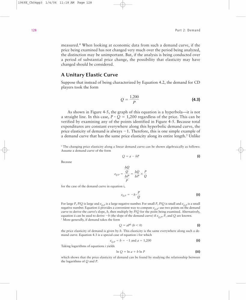
measured.4 When looking at economic data from such a demand curve, if theprice being examined has not changed very much over the period being analyzed,the distinction may be unimportant. But, if the analysis is being conducted overa period of substantial price change, the possibility that elasticity may havechanged should be considered.

A Unitary Elastic CurveSuppose that instead of being characterized by Equation 4.2, the demand for CDplayers took the form

{4.3}

As shown in Figure 4-5, the graph of this equation is a hyperbola—it is nota straight line. In this case, P ? Q 5 1,200 regardless of the price. This can beverified by examining any of the points identified in Figure 4-5. Because totalexpenditures are constant everywhere along this hyperbolic demand curve, theprice elasticity of demand is always 21. Therefore, this is one simple example ofa demand curve that has the same price elasticity along its entire length.5 Unlike

Q 51,200

P

128 P a r t 2 : D e m a n d

4 The changing price elasticity along a linear demand curve can be shown algebraically as follows:Assume a demand curve of the form

Q 5 a 2 bP {i}

Because

for the case of the demand curve in equation i,

{ii}

For large P, P/Q is large and eQ,P is a large negative number. For small P, P/Q is small and eQ,P is a smallnegative number. Equation ii provides a convenient way to compute eQ,P: use two points on the demandcurve to derive the curve’s slope, b, then multiply by P/Q for the point being examined. Alternatively,equation ii can be used to derive 2b (the slope of the demand curve) if eQ,P, P, and Q are known.5 More generally, if demand takes the form

Q 5 aPb (b , 0) {i}

the price elasticity of demand is given by b. This elasticity is the same everywhere along such a de-mand curve. Equation 4.3 is a special case of equation i for which

eQ,P 5 b 5 21 and a 5 1,200 {ii}

Taking logarithms of equations i yields

ln Q 5 ln a 1 b ln P {iii}

which shows that the price elasticity of demand can be found by studying the relationship betweenthe logarithms of Q and P.

eQ,P 5 2b ?

PQ

eQ,P 5

DQQ

DPP

5DQDP

3PQ

1969X_Ch04pp3 1/4/06 11:18 AM Page 128

C h a p t e r 4 : M a r k e t D e m a n d a n d E l a s t i c i t y 129

the linear case, for this curve, there is no need to worry about being specificabout the point at which elasticity is to be measured. Application 4.4: An Exper-iment in Health Insurance illustrates how you might calculate elasticity fromactual data and why your results could be very useful indeed.

I INCOME ELASTICITY OF DEMAND

Another type of elasticity is the income elasticity of demand (eQ,I). This con-cept records the relationship between changes in income and changes in quantitydemanded:

{4.4}

For a normal good, eQ,I is positive because increases in income lead to in-creases in purchases of the good. For the unlikely case of an inferior good, on theother hand, eQ,I would be negative, implying that increases in income lead to de-creases in quantity purchased. Such negative income elasticities are rarely en-countered, however.

Among normal goods, whether eQ,I is greater than or less than 1 is a matterof some interest. Goods for which eQ,I . 1 might be called luxury goods, in thatpurchases of these goods increase more rapidly than income. For example, ifthe income elasticity of demand for automobiles is 2, then a 10 percent increase

Income elasticity of demand 5 eQ,I 5Percentage change in QPercentage change in I

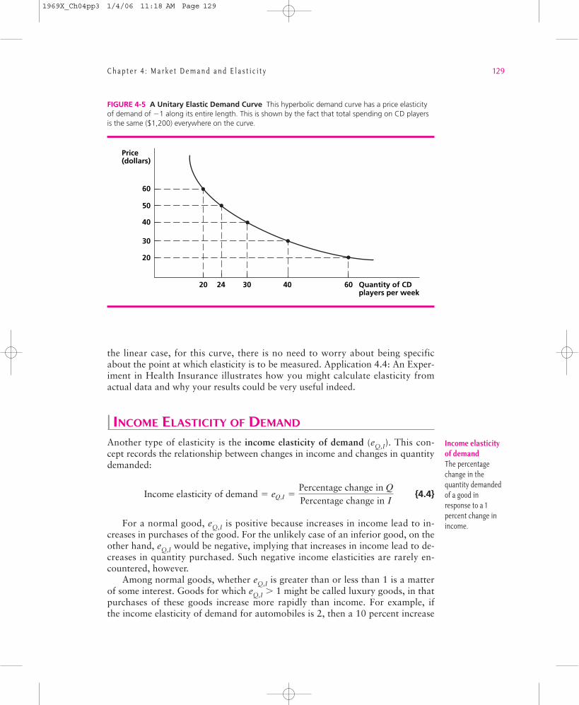
FIGURE 4-5 A Unitary Elastic Demand Curve This hyperbolic demand curve has a price elasticityof demand of 21 along its entire length. This is shown by the fact that total spending on CD playersis the same ($1,200) everywhere on the curve.

Price(dollars)

20

60

50

40

30

Quantity of CDplayers per week

20 24 30 40 60

Income elasticityof demandThe percentagechange in thequantity demandedof a good inresponse to a 1percent change inincome.

1969X_Ch04pp3 1/4/06 11:18 AM Page 129

130 P a r t 2 : D e m a n d

The provision of health insurance is one of the mostuniversal and expensive social policies throughoutthe world. Although many nations have compre-hensive insurance schemes that cover most of theirpopulations, policymakers in the United States haveresisted such an all-inclusive approach. Instead, U.S.policies have evolved as a patchwork, stressingemployer-provided insurance for workers togetherwith special programs for the aged (Medicare) andthe poor (Medicaid). Regardless of how health in-surance plans are designed, however, all face a sim-ilar set of problems.

Moral HazardOne of the most important such problems is thatinsurance coverage of health care needs tends toincrease the demand for services. Because insuredpatients pay only a small fraction of the costs of theservices they receive, they will demand more thanthey would have if they had to pay market prices.This tendency of insurance coverage to increase de-mand is (perhaps unfortunately) called “moral haz-ard,” though there is nothing especially immoralabout such behavior.

The Rand ExperimentThe Medicare program was introduced in theUnited States in 1965, and the increase in demandfor medical services by the elderly was immediatelyapparent. In order to understand better the factorsthat were leading to this increase in demand, thegovernment funded a large-scale experiment infour cities. In that experiment, which was con-ducted by the Rand Corporation, people were as-signed to different insurance plans that varied inthe fraction of medical costs that people wouldhave to pay out of their own pockets for medicalcare.1 In insurance terms, the experiment varied the“coinsurance” rate from zero (free care) to nearly100 percent (patients pay everything).

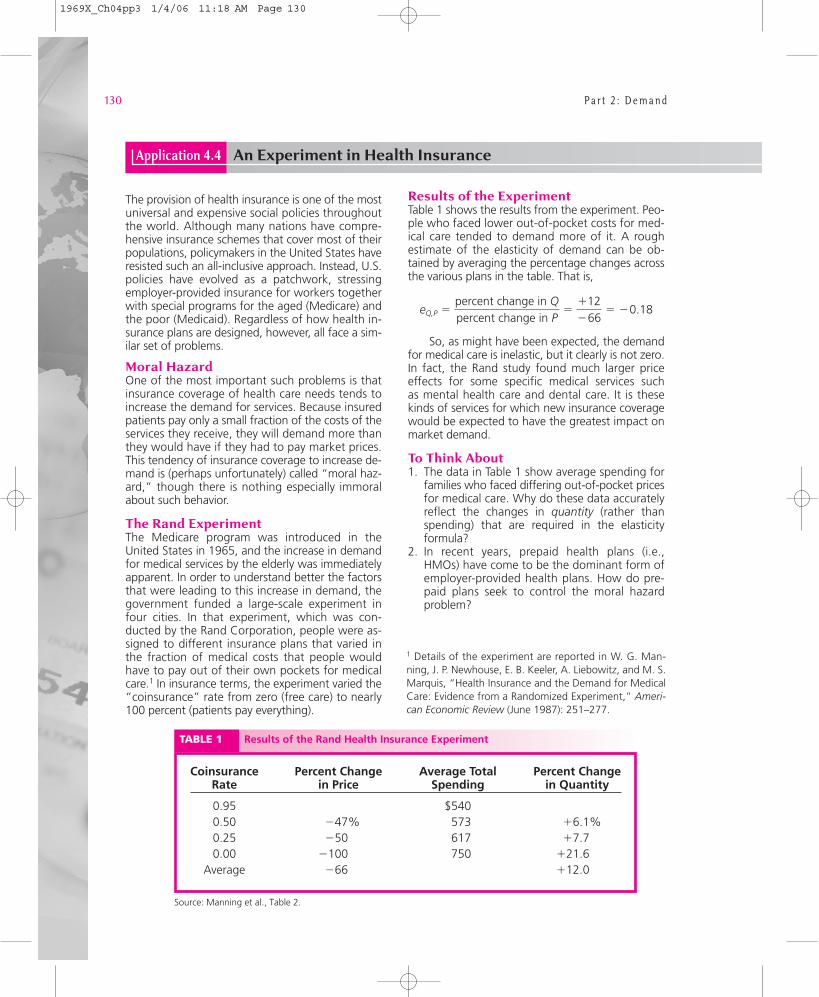
Results of the ExperimentTable 1 shows the results from the experiment. Peo-ple who faced lower out-of-pocket costs for med-ical care tended to demand more of it. A roughestimate of the elasticity of demand can be ob-tained by averaging the percentage changes acrossthe various plans in the table. That is,

So, as might have been expected, the demandfor medical care is inelastic, but it clearly is not zero.In fact, the Rand study found much larger priceeffects for some specific medical services suchas mental health care and dental care. It is thesekinds of services for which new insurance coveragewould be expected to have the greatest impact onmarket demand.

To Think About1. The data in Table 1 show average spending for

families who faced differing out-of-pocket pricesfor medical care. Why do these data accuratelyreflect the changes in quantity (rather thanspending) that are required in the elasticityformula?

2. In recent years, prepaid health plans (i.e.,HMOs) have come to be the dominant form ofemployer-provided health plans. How do pre-paid plans seek to control the moral hazardproblem?

eQ,P 5percent change in Qpercent change in P

5112266

5 20.18

Application 4.4 An Experiment in Health Insurance

1 Details of the experiment are reported in W. G. Man-ning, J. P. Newhouse, E. B. Keeler, A. Liebowitz, and M. S.Marquis, “Health Insurance and the Demand for MedicalCare: Evidence from a Randomized Experiment,” Ameri-can Economic Review (June 1987): 251–277.

TABLE 1 Results of the Rand Health Insurance Experiment

Source: Manning et al., Table 2.

Coinsurance Percent Change Average Total Percent ChangeRate in Price Spending in Quantity

0.95 $5400.50 247% 573 16.1%0.25 250 617 17.70.00 2100 750 121.6

Average 266 112.0

1969X_Ch04pp3 1/4/06 11:18 AM Page 130

C h a p t e r 4 : M a r k e t D e m a n d a n d E l a s t i c i t y 131

in income will lead to a 20 percent increase inautomobile purchases. Auto sales would there-fore be very responsive to business cycles thatproduce changes in people’s incomes. On theother hand Engel’s Law suggests that food hasan income elasticity of much less than 1. If theincome elasticity of demand for food were 0.5,for example, then a 10 percent rise in incomewould result in only a 5 percent increase in foodpurchases. Considerable research has been doneto determine the actual values of income elastic-ities for various items, and we discuss the resultsof some of these studies in the final section ofthis chapter.

I CROSS-PRICE ELASTICITY OF DEMAND

In Chapter 3 we showed that a change in the price of one good will affect thequantity demanded of many other goods. To measure such effects, economistsuse the cross-price elasticity of demand. This concept records the percentagechange in quantity demanded (Q) that results from a 1 percentage point changein the price of some other good (call this other price P9). That is,

(4.5)

If the two goods in question are substitutes, the cross-price elasticity of demandwill be positive because the price of one good and the quantity demanded of theother good will move in the same direction. For example, the cross-price elastic-ity for changes in the price of tea on coffee demand might be 0.2. Each 1 percent-

age point increase in the price of tea results in a0.2 percentage point increase in the demand forcoffee because coffee and tea are substitutes inpeople’s consumption choices. A fall in theprice of tea would cause the demand for coffeeto fall also, since people would choose to drinktea rather than coffee.

If two goods in question are complements,the cross-price elasticity will be negative, show-ing that the price of one good and the quantityof the other good move in opposite directions.The cross-price elasticity of doughnut prices oncoffee demand might be, say, 21.5. This wouldimply that each 1 percent increase in the price ofdoughnuts would cause the demand for coffee

Cross-price elasticity of demand 5 eQ,P 5 Percentage change in QPercentage change in P

Cross-priceelasticity ofdemandThe percentagechange in thequantity demandedof a good inresponse to a 1percent change inthe price of anothergood.

Possible values for the income elasticity of de-mand are restricted by the fact that consumersare bound by budget constraints. Use this fact toexplain:

1. Why is it that not every good can have an in-come elasticity of demand greater than 1? Canevery good have an income elasticity of demandless than 1?

2. If a set of consumers spend 95 percent oftheir incomes on housing, why can’t the incomeelasticity of demand for housing be muchgreater than 1?

M I C R O Q U I Z 4 . 3

Suppose that a set of consumers spend their in-comes only on beer and pizza.

1. Explain why a fall in the price of beer will havean ambiguous effect on pizza purchases.

2. What can you say about the relationship be-tween the price elasticity of demand for pizza,the income elasticity of demand for pizza, andthe cross-price elasticity of the demand for pizzawith respect to beer prices? (Hint: Rememberthe demand for pizza must be homogeneous.)

M I C R O Q U I Z 4 . 4

1969X_Ch04pp3 1/18/06 2:06 PM Page 131

to fall by 1.5 percent. When doughnuts are more expensive, it becomes less attrac-tive to drink coffee because many people like to have a doughnut with their morn-ing coffee. A fall in the price of doughnuts would increase coffee demand because,in that case, people will choose to consume more of both complementary products.As for the other elasticities we have examined, considerable empirical research hasbeen conducted to try to measure actual cross-price elasticities of demand.

I EMPIRICAL STUDIES

I OF DEMAND

Economists have for many years studied the demand for all sorts of goods. Someof the earliest studies generalized from the expenditure patterns of a small sam-ple of families. More recent studies have examined a wide variety of goods to es-timate both income and price elasticities. Although it is not possible for us todiscuss in detail here the statistical techniques used in these studies, we can showin a general way how these economists have gone about getting their estimates.

Estimating Demand CurvesEstimating the demand curve for a product is one of the more difficult and im-portant problems in econometrics. The importance of the question is obvious.Without some idea of what the demand curve for a product looks like, econo-mists could not describe with any precision how the market for a good might beaffected by various events. Usually the notion that a rise in price will cause quan-tity demanded to fall will not be precise enough—we need some way to estimatethe size of the effect.

Problems in deriving such an estimate are of two general types. First are thoserelated to the need to implement the ceteris paribus assumption. One must findsome way to hold constant all of the other factors that affect quantity demandedso that the direct relationship between price and quantity can be observed. Oth-erwise, we will be looking at points on several demand curves rather than ononly one. We have already discussed this problem in the Appendix to Chapter 1,which shows how it can often be solved through the use of relatively simple sta-tistical procedures.6

A second problem in estimating a demand curve goes to the heart of micro-economic theory. From the early days in your introductory economics course,you have (hopefully) learned that quantity and price are determined by the simul-taneous operation of demand and supply. A simple plot of quantity versus pricewill be neither a demand curve nor a supply curve, but only points at which thetwo curves intersect. The econometric problem then is to penetrate behind thisconfusion and “identify” the true demand curve. There are indeed methods for

132 P a r t 2 : D e m a n d

www.infotrac-college.comKeywords: Priceelasticity, Farmprices, Rand healthinsuranceexperiment, Moralhazard

6 The most common technique, multiple regression analysis, estimates a relationship between quantitydemanded (Q), price (P), and other factors that affect quantity demanded (X) of the form Q 5 a 1 bP1 cX. Given this relationship, X can be held constant while looking at the relationship between Q andP. Following footnote 5, it is common practice to use logarithms to provide estimates of elasticities.

1969X_Ch04pp3 1/18/06 2:06 PM Page 132

doing this, though we will not pursue them here.7 All studies of demand, includ-ing those we look at in the next section, must address this issue, however.

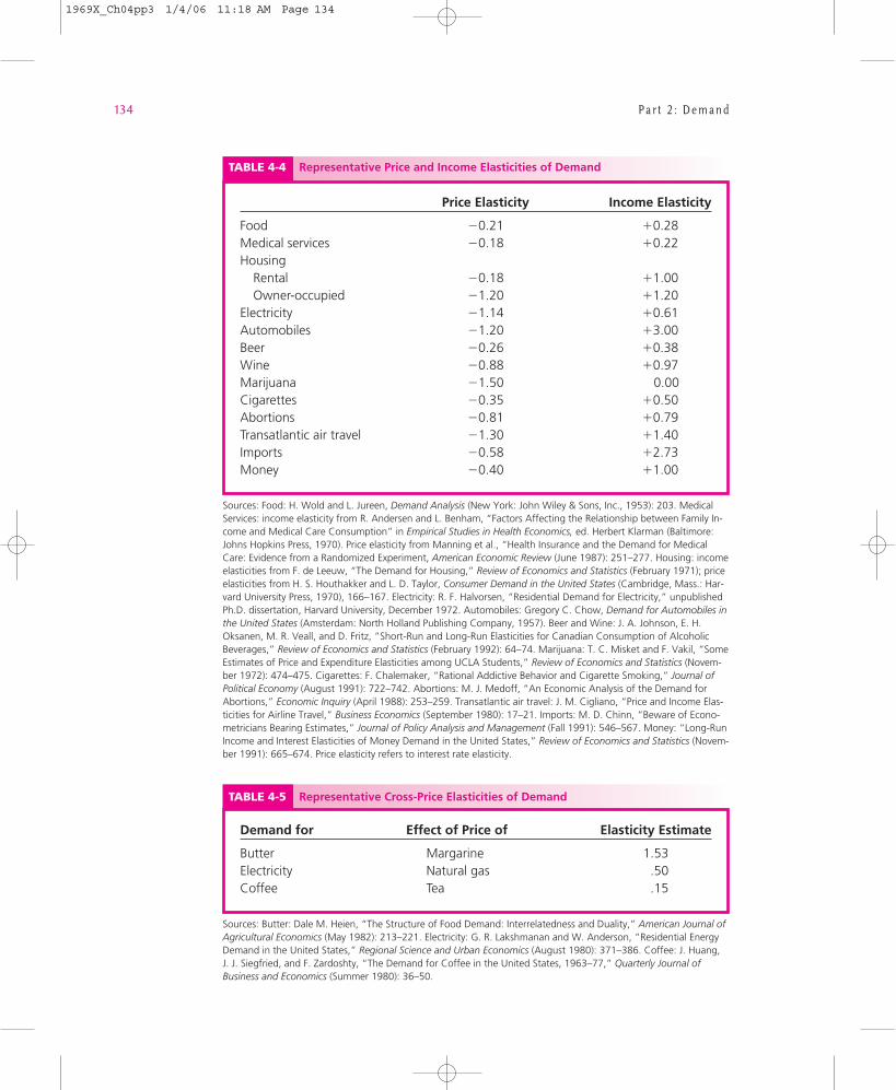
Some Elasticity EstimatesTable 4-4 gathers a number of estimated income and price elasticities of demand.As we shall see, these estimates often provide the starting place for analyzing howactivities such as changes in taxes or import policy might affect various markets.In several later chapters, we use these numbers to illustrate such applications.

Although interested readers are urged to explore the original sources of theseestimates to understand more details about them, in our discussion we just takenote of a few regularities they exhibit. With regard to the price elasticity figures,most estimates suggest that product demands are relatively inelastic (between0 and 21). For the groupings of commodities listed, substitution effects are notespecially large, although they may be large within these categories. For example,substitutions between beer and other commodities may be relatively small, thoughsubstitutions among brands of beer may be substantial in response to price differ-ences. Still, all the estimates are less than 0, so there is clear evidence that peopledo respond to price changes for most goods.8 Application 4.5: Alcohol Taxes asDrunk Driving Policy shows how price elasticity estimates can inform an impor-tant policy debate.

As expected, the income elasticities in Table 4-4 are positive and are roughlycentered about 1.0. Luxury goods, such as automobiles or transatlantic travel(eQ,I . 1), tend to be balanced by necessities, such as food or medical care(eQ,I , 1). Because none of the income elasticities are negative, it is clear thatGiffen’s paradox must be very rare.

Some Cross-Price Elasticity EstimatesTable 4-5 shows a few cross-price elasticity estimates that economists have de-rived. All of the pairs of goods illustrated are probably substitutes, and the posi-tive values for the elasticities confirm that view. The figure for the relationshipbetween butter and margarine is the largest in Table 4-5. Even in the absence ofhealth issues, the competition between these two spreads on the basis of price isclearly very intense. Similarly, natural gas prices have an important effect on elec-tricity sales because they help determine how people heat their homes.

C h a p t e r 4 : M a r k e t D e m a n d a n d E l a s t i c i t y 133

7 For a good discussion, see R. Ramanathan, Introductory Econometrics with Applications, 5th ed.(Mason, OH: South-Western, 2002), Chapter 13.8 Although the estimated price elasticities in Table 4-4 incorporate both substitution and income ef-fects, they predominantly represent substitution effects. To see this, note that the price elasticity ofdemand (eQ,P) can be disaggregated into substitution and income effects by

eQ,P 5 eS 2 siei

where eS is the “substitution” price elasticity of demand representing the effect of a price changeholding utility constant, si is the share of income spent on the good in question, and ei is the good’sincome elasticity of demand. Because si is small for most of the goods in Table 4-4, eQ,P and eS havevalues that are reasonably close.

1969X_Ch04pp3 1/4/06 11:18 AM Page 133

134 P a r t 2 : D e m a n d

TABLE 4-5 Representative Cross-Price Elasticities of Demand

Sources: Butter: Dale M. Heien, “The Structure of Food Demand: Interrelatedness and Duality,” American Journal ofAgricultural Economics (May 1982): 213–221. Electricity: G. R. Lakshmanan and W. Anderson, “Residential EnergyDemand in the United States,” Regional Science and Urban Economics (August 1980): 371–386. Coffee: J. Huang,J. J. Siegfried, and F. Zardoshty, “The Demand for Coffee in the United States, 1963–77,” Quarterly Journal ofBusiness and Economics (Summer 1980): 36–50.

Demand for Effect of Price of Elasticity Estimate

Butter Margarine 1.53Electricity Natural gas .50Coffee Tea .15

TABLE 4-4 Representative Price and Income Elasticities of Demand

Sources: Food: H. Wold and L. Jureen, Demand Analysis (New York: John Wiley & Sons, Inc., 1953): 203. MedicalServices: income elasticity from R. Andersen and L. Benham, “Factors Affecting the Relationship between Family In-come and Medical Care Consumption” in Empirical Studies in Health Economics, ed. Herbert Klarman (Baltimore:Johns Hopkins Press, 1970). Price elasticity from Manning et al., “Health Insurance and the Demand for MedicalCare: Evidence from a Randomized Experiment, American Economic Review (June 1987): 251–277. Housing: incomeelasticities from F. de Leeuw, “The Demand for Housing,” Review of Economics and Statistics (February 1971); priceelasticities from H. S. Houthakker and L. D. Taylor, Consumer Demand in the United States (Cambridge, Mass.: Har-vard University Press, 1970), 166–167. Electricity: R. F. Halvorsen, “Residential Demand for Electricity,” unpublishedPh.D. dissertation, Harvard University, December 1972. Automobiles: Gregory C. Chow, Demand for Automobiles inthe United States (Amsterdam: North Holland Publishing Company, 1957). Beer and Wine: J. A. Johnson, E. H.Oksanen, M. R. Veall, and D. Fritz, “Short-Run and Long-Run Elasticities for Canadian Consumption of AlcoholicBeverages,” Review of Economics and Statistics (February 1992): 64–74. Marijuana: T. C. Misket and F. Vakil, “SomeEstimates of Price and Expenditure Elasticities among UCLA Students,” Review of Economics and Statistics (Novem-ber 1972): 474–475. Cigarettes: F. Chalemaker, “Rational Addictive Behavior and Cigarette Smoking,” Journal ofPolitical Economy (August 1991): 722–742. Abortions: M. J. Medoff, “An Economic Analysis of the Demand forAbortions,” Economic Inquiry (April 1988): 253–259. Transatlantic air travel: J. M. Cigliano, “Price and Income Elas-ticities for Airline Travel,” Business Economics (September 1980): 17–21. Imports: M. D. Chinn, “Beware of Econo-metricians Bearing Estimates,” Journal of Policy Analysis and Management (Fall 1991): 546–567. Money: “Long-RunIncome and Interest Elasticities of Money Demand in the United States,” Review of Economics and Statistics (Novem-ber 1991): 665–674. Price elasticity refers to interest rate elasticity.

Price Elasticity Income Elasticity

Food 20.21 10.28Medical services 20.18 10.22Housing

Rental 20.18 11.00Owner-occupied 21.20 11.20

Electricity 21.14 10.61Automobiles 21.20 13.00Beer 20.26 10.38Wine 20.88 10.97Marijuana 21.50 0.00Cigarettes 20.35 10.50Abortions 20.81 10.79Transatlantic air travel 21.30 11.40Imports 20.58 12.73Money 20.40 11.00

1969X_Ch04pp3 1/4/06 11:18 AM Page 134

Each year more than 40,000 Americans die in auto-mobile accidents. Such accidents are the leadingcause of death for teenagers. It is generally believedthat alcohol consumption is a major factor in atleast half of those accidents. In recent years, thegovernment has tried to combat drunk driving byteenagers in two primary ways: by increasing legalminimum ages for drinking and by adopting stricterdrunk-driving laws. These efforts appear to havehad significant effects in reducing teen fatalities. Atthe same time that these laws were coming into ef-fect, however, real taxes on alcohol declined. Be-cause teens may be especially sensitive to alcoholprices, these reductions may have eroded some ofthe impact of the more stringent laws. But theconnection between teen alcohol consumption andalcohol taxes is actually more complex than it firstappears.

Price Elasticity Estimates—The Importance of BeerMost empirical studies of alcohol consumptionshow that it is sensitive to price. The figures in Table4-4 suggest that these elasticities in the UnitedStates range from approximately 20.3 for beer toperhaps as large as 20.9 for wine. Studies of alco-hol consumption in other countries reach essentiallythe same conclusion: while all alcohol consumptionappears to be relatively price sensitive, price elastici-ties for beer are usually found to be less than halfthose for wine (and other spirits). Unfortunately,most teenage alcohol consumption is beer. Thelower price elasticity of demand for this producttherefore poses a problem for those who would usealcohol taxes as a deterrent to drunk driving.

Why beer should have a lower price elasticity ofdemand than other alcoholic beverages is a puzzle.Two factors may provide a partial explanation. First,a significant portion of beer consumption is done ina group setting (tapping a keg, for example). In thiscase, the direct impact of higher prices may be lessthan when goods are purchased individually be-cause, at the margin, drinking more costs the con-sumer no more in out-of-pocket costs. A secondpossible reason for the lower price elasticity of beerconsumption relates to differences among beerconsumers. Most beer is consumed by people whodrink quite a bit of it (say, more than a six-pack at asession). This is a group of consumers for whom de-mand has been found to be less responsive to pricethan is the case for most other consumers.

Beer Consumption and Habit FormationAnother possibility, however, is that past studiesof alcohol consumption have not modeled this ac-tivity correctly, and thus consumption may be moreprice responsive than the elasticity estimates imply.Specifically, some authors have argued that “binge”drinking of beer is primarily a habit, created overseveral years of increasingly serious drinking. Hence,as for many products, the price elasticity of demandfor beer may be much larger over the long run thanthe short-run estimates imply. One importanteconometric study that supports this conclusionfinds that restoring the real rate of taxation on beerto that prevailing in the 1970s would reduce high-way fatalities by 7 to 8 percent—a figure about inline with the declines brought on by the stricterlaws.1 Overall, such a price increase might saveabout 3,500 lives.

A similar conclusion was reached by C. Carpen-ter who looked at the importance of habit forma-tion in another way.2 The author studied the impactof “zero-tolerance” drunk driving laws that set verylow blood alcohol limits for drivers under 21. Heshowed that these laws reduced binge drinkingby about 13 percent among younger males—anestimate close to that found for the impact ofhigher beer prices. Because this study was based onself-reported alcohol use, however, the author hadsome difficulty in tying his findings of reduceddrinking to actual reductions in drunk driving.

To Think About1. Reducing alcohol consumption through taxation

would have a number of effects in addition tothose related to drunk driving. What are some ofthese effects? Do these also provide a rationalefor higher alcohol taxes?

2. One principle of efficient taxation is that taxesshould be imposed directly on the “problem.”Alcohol taxes do not do that because they tax al-cohol consumers who do not drive and they donot tax nondrinkers who cause accidents. Still,why might this policy be preferred to a more di-rect tax on drunk drivers?

C h a p t e r 4 : M a r k e t D e m a n d a n d E l a s t i c i t y 135

Application 4.5 Alcohol Taxes as Drunk Driving Policy

1 C. J. Ruhm, “Alcohol Policies and Highway Vehicle Fa-talities,” Journal of Health Economics (August 1996):435–454.2 C. Carpenter, “How Do Zero Tolerance Drunk DrivingLaws Work?” Journal of Health Economics, January, 2004:61–83.

1969X_Ch04pp3 1/4/06 11:18 AM Page 135

136 P a r t 2 : D e m a n d

In this chapter, we constructed a market demandcurve by adding up the demands of all potentialconsumers. This curve shows the relationship be-tween the market price of a good and the amountthat people choose to purchase of that good, assum-ing all the other factors that affect demand do notchange. The market demand curve is a basic build-ing block for the theory of price determination. Weuse the concept frequently throughout the remain-der of this book. You should therefore keep in mindthe following points about this concept:

• The market demand curve represents the summa-tion of the demands of a given number of poten-tial consumers of a particular good. The curveshows the ceteris paribus relationship betweenthe market price of the good and the amount de-manded by all consumers.

• Factors that shift individual demand curves alsoshift the market demand curve to a new position.Such factors include changes in incomes, changesin the prices of other goods, and changes in peo-ple’s preferences.

• The price elasticity of demand provides a con-venient way of measuring the extent to whichmarket demand responds to price changes formovement along a given demand curve. Specifi-cally, the price elasticity of demand shows the

percentage change in quantity demanded in re-sponse to a 1 percent change in market price.Demand is said to be elastic if a 1 percent changein price leads to a greater than 1 percent changein quantity demanded. Demand is inelastic if a 1 percent change in price leads to a smaller than1 percent change in quantity.

• There is a close relationship between the priceelasticity of demand and total spending on agood. If demand is elastic, a rise in price will re-duce total expenditures. If demand is inelastic, arise in price will increase total spending.

• Other elasticities of demand are defined in a waysimilar to that used for the price elasticity. For ex-ample, the income elasticity of demand measuresthe percentage change in quantity demanded inresponse to a 1 percent change in income.

• The price elasticity of demand is not necessarilythe same at every point on a demand curve. For alinear demand curve, demand is elastic for highprices and inelastic for low prices.

• Economists have estimated elasticities of demandfor many different goods using real-world data. Amajor problem in making such estimates is to de-vise ways of holding constant all other factorsthat affect demand so that the price2quantitypoints being used lie on a single demand curve.

SUMMARY

1. In the construction of the market demand curveshown in Figure 4-1, why is a horizontal linedrawn at the prevailing price, ? What does this assume about the price facing each person?How are people assumed to react to this price?

2. Explain how the following events might affectthe market demand curve for prime filet mignon:a. A fall in the price of filet mignon because of

a decline in cattle pricesb. A general rise in consumers’ incomesc. A rise in the price of lobsterd. Increased health concerns about cholesterol

e. An income tax increase for high-income peo-ple, used to increase welfare benefits

f. A cut in income taxes and welfare benefits3. Why is the price elasticity of demand usually

negative? If the price elasticity of demand forautomobiles is less than the price elasticity ofdemand for medical care, which demand ismore elastic? Give a numerical example.

4. “Gaining extra revenue is easy for any pro-ducer—all it has to do is raise the price of itsproduct.” Do you agree? Explain when thiswould be true and when it would not be true.

P*x

REVIEW QUESTIONS

1969X_Ch04pp3 1/4/06 11:18 AM Page 136

C h a p t e r 4 : M a r k e t D e m a n d a n d E l a s t i c i t y 137

5. Suppose that the market demand curve forpasta is a straight line of the form Q 5 300 250P where Q is the quantity of pasta bought inthousands of boxes per week and P is the priceper box (in dollars).a. At what price does the demand for pasta go

to 0? Develop a numerical example to showthat the demand for pasta is elastic at thispoint.

b. How much pasta is demanded at a price of$0? Develop a numerical example to showthat demand is inelastic at this point.

c. How much pasta is demanded at a price of$3? Develop a numerical example that sug-gests that total spending on pasta is as largeas possible at this price.

6. Marvin currently spends 35 percent of his$100,000 income on housing. If his income elas-ticity of demand for housing is 0.8, will this frac-tion rise or fall when he gets a raise to $120,000?What is the new fraction of income spent onhousing? Would you give different answers tothe questions if Marvin’s income elasticity ofdemand for housing were 1.3?

7. J. Trueblue always spends one-third of his in-come on American flags. What is the income

elasticity of his demand for such flags? What isthe price elasticity of his demand for flags?

8. Table 4-4 reports an estimated price elasticity ofdemand for electricity of 21.14. Explain whatthis means with a numerical example. Does thisnumber seem large? Do you think this is a short-or long-term elasticity estimate? How might thisestimate be important for owners of electric utili-ties or for bodies that regulate them?

9. Table 4-5 reports that the cross-price elasticity ofdemand for electricity with respect to the price ofnatural gas is 0.50. Explain what this means witha numerical example. What does the fact that thenumber is positive imply about the relationshipbetween electricity and natural gas use?

10. An economist hired by a home building firmhas been asked to estimate a demand curve forhomes. He gathers data on the price of newhouses and on the number sold from the top100 metropolitan areas in the United States.He plots these data, draws a line that seems topass near the points, and labels that line “de-mand.” How many problems can you identifyin this approach to estimating the demand forhouses?

4.1 Suppose the demand curve for flyswatters isgiven by

Q 5 500 2 50P

where Q is the number of flyswatters demanded perweek and P is the price in dollars.

a. How many flyswatters are demanded at a price of$2? How about a price of $3? $4? Suppose fly-swatters were free; how many would be bought?

b. Graph the flyswatter demand curve. Rememberto put P on the vertical axis and Q on the hori-zontal axis. To do so, you may wish to solve forP as a function of Q.

c. Suppose during July the flyswatter demand curveshifts to

Q 5 1,000 2 50P

Answer part a and part b for this new demand curve.

4.2 Suppose that the demand curve for garbanzobeans is given by

Q 5 20 2 P

where Q is thousands of pounds of beans boughtper week and P is the price in dollars per pound.

a. How many beans will be bought at P 5 0?

PROBLEMS

1969X_Ch04pp3 1/4/06 11:18 AM Page 137

138 P a r t 2 : D e m a n d

b. At what price does the quantity demanded ofbeans become 0?

c. Calculate total expenditures (P ? Q) for beans ofeach whole dollar price between the prices iden-tified in part a and part b.

d. What price for beans yields the highest totalexpenditures?

e. Suppose the demand for beans shifted to Q 5

40 2 2P. How would your answers to part athrough part d change? Explain the differencesintuitively and with a graph.

4.3 Consider the three demand curves

{i}

{ii}

{iii}

a. Use a calculator to compute the value of Q foreach demand curve for P 5 1 and for P 5 1.1.

b. What do your calculations show about the priceelasticity of demand at P 5 1 for each of thethree demand curves?

c. Now perform a similar set of calculations for thethree demand curves at P 5 4 and P 5 4.4. Howdo the elasticities computed here compare tothose from part b? Explain your results usingfootnote 5 of this chapter.

4.4 The market demand for potatoes is given by

Q 5 1,000 1 0.3I 2 300P 1 299P9

where

Q 5 Annual demand in poundsI 5 Average income in dollars per yearP 5 Price of potatoes in cents per pound

P9 5 Price of rice in cents per pound.

a. Suppose I 5 $10,000 and P9 5 $0.25; whatwould be the market demand for potatoes? At

what price would Q 5 0? Graph this demandcurve.

b. Suppose I rose to $20,000 with P9 staying at$0.25. Now what would the demand for potatoesbe? At what price would Q 5 0? Graph this de-mand curve. Explain why more potatoes are de-manded at every price in this case than in part a.

c. If I returns to $10,000 but P9 falls to $0.10, whatwould the demand for potatoes be? At what pricewould Q 5 0? Graph this demand curve. Explainwhy fewer potatoes are demanded at every pricein this case than in part a.

4.5 Tom, Dick, and Harry constitute the entiremarket for scrod. Tom’s demand curve is given by

Q1 5 100 2 2P

for P # 50. For P . 50, Q1 5 0. Dick’s demandcurve is given by

Q2 5 160 2 4P

for P # 40. For P . 40, Q2 5 0. Harry’s demandcurve is given by

Q3 5 150 2 5P

for P # 30. For P . 30, Q3 5 0. Using this infor-mation, answer the following:

a. How much scrod is demanded by each person atP 5 50? At P 5 35? At P 5 25? At P 5 10? Andat P 5 0?

b. What is the total market demand for scrod ateach of the prices specified in part a?

c. Graph each individual’s demand curve.d. Use the individual demand curves and the results

of part b to construct the total market demandfor scrod.

4.6 Suppose the quantity of good X demanded byindividual 1 is given by

X1 5 10 2 2PX 1 0.01I1 1 0.4PY

and the quantity of X demanded by individual 2 is

X2 5 5 2 PX 1 0.02I2 1 0.2PY

a. What is the market demand function for total

Q 5100P 3 >2

Q 5100

"P

Q 5100P

1969X_Ch04pp3 1/4/06 11:18 AM Page 138

C h a p t e r 4 : M a r k e t D e m a n d a n d E l a s t i c i t y 139

X (5 X1 1 X2) as a function of PX, I1, I2, andPY?

b. Graph the two individual demand curves (with Xon the horizontal axis, PX on the vertical axis) forthe case I1 5 1,000, I2 5 1,000, and PY 5 10.

c. Using these individual demand curves, constructthe market demand curve for total X. What isthe algebraic equation for this curve?

d. Now suppose I1 increases to 1,100 and I2 de-creases to 900. How would the market demandcurve shift? How would the individual demandcurves shift? Graph these new curves.

e. Finally, suppose PY rises to 15. Graph the newindividual and market demand curves thatwould result.

4.7 Suppose that the current market price of VCRsis $300, that average consumer disposable incomeis $30,000, and that the price of DVD players (asubstitute for VCRs) is $500. Under these condi-tions, the annual U.S. demand for VCRs is 5 millionper year. Statistical studies have shown that for thisproduct eQ,P 5 21.3, eQ,I 5 1.7, and eQ,P9 5 0.8where P9 is the price of DVD players.

Use this information to predict the annual numberof VCRs sold under the following conditions:

a. Increasing competition from Korea causes VCRprices to fall to $270 with I and P9 unchanged.

b. Income tax reductions raise average disposableincome to $31,500 with P and P9 unchanged.

c. Technical improvements in DVD players causetheir price to fall to $400 with P and I un-changed.

d. All of the events described in part a through partc occur simultaneously.

4.8 In Chapter 3 we introduced the concept of con-sumer surplus as measured by the area above mar-ket price and below an individual’s demand for agood. This problem asks you to think about thatconcept for the market as a whole.

a. Consumer surplus in the market as a whole issimply the sum of the consumer surplus receivedby each individual consumer. Use Figure 4-1 toexplain why this total consumer surplus is alsogiven by the area under the market demandcurve and above the current price.

b. Use a graph to show that the loss of consumersurplus resulting from a given price rise is greaterwith an inelastic demand curve than with anelastic one. Explain your result intuitively. (Hint:What is the primary reason a demand curve iselastic?)

c. How would you evaluate the following assertion:“The welfare loss from any price increase can bereadily measured by the increased spending on agood made necessary by that price increase.”

4.9 In Problem 3.9, we introduced compensated de-mand curves along which utility is held constantand only the substitution effect of price changes isconsidered. This problem shows how the price elas-ticity of demand along such a curve is related to thecustomary measure of price elasticity.

a. Suppose consumers buy only two goods, foodand shelter, and that they buy these in fixedproportions—one unit of food for each unitof shelter. In this case, what does the compen-sated demand curve for food look like? What isthe price elasticity of demand along this curve(call this elasticity es—the substitution elastic-ity)? Are there any substitution effects in thisdemand?

b. Under the conditions of part a, what is the in-come elasticity of demand for food (eF,I)?

c. Continuing as in part a, suppose one unit offood costs half what one unit of housing costs.What fraction of income will be spent on food(call this sF)?

d. Using the information in part c, what is the over-all price elasticity of demand (including bothsubstitution and income effects) for food (eF,P)?(Hint: A numerical example may help here.)

e. Use your answers to part a through part dto show that the numbers calculated in thisproblem obey the formula in footnote 8 of thischapter:

eF,P 5 es 2 sFeF,I

This formula is quite general. It is some-times called the “Slutsky Equation” after its dis-coverer.

f. Let us change this problem a bit now to assumethat people always spend 1⁄3 of their income onfood, no matter what their income or what the

1969X_Ch04pp3 1/4/06 11:18 AM Page 139

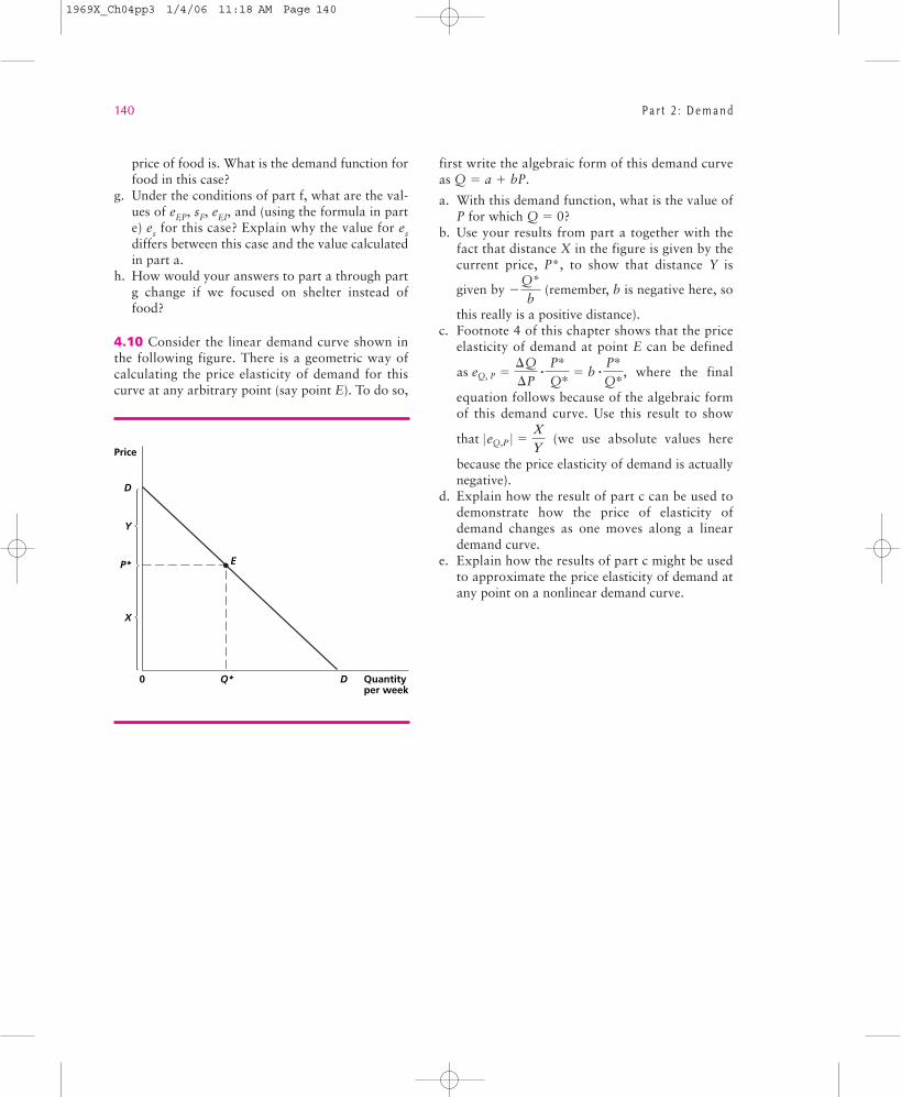
140 P a r t 2 : D e m a n d

price of food is. What is the demand function forfood in this case?

g. Under the conditions of part f, what are the val-ues of eF,P, sF, eF,I, and (using the formula in parte) es for this case? Explain why the value for esdiffers between this case and the value calculatedin part a.

h. How would your answers to part a through partg change if we focused on shelter instead offood?

4.10 Consider the linear demand curve shown inthe following figure. There is a geometric way ofcalculating the price elasticity of demand for thiscurve at any arbitrary point (say point E). To do so,

first write the algebraic form of this demand curveas .

a. With this demand function, what is the value ofP for which Q 5 0?

b. Use your results from part a together with thefact that distance X in the figure is given by thecurrent price, P*, to show that distance Y is

given by 2 (remember, b is negative here, so

this really is a positive distance).c. Footnote 4 of this chapter shows that the price

elasticity of demand at point E can be defined

as , where the final

equation follows because of the algebraic formof this demand curve. Use this result to show

that (we use absolute values here

because the price elasticity of demand is actuallynegative).

d. Explain how the result of part c can be used todemonstrate how the price of elasticity ofdemand changes as one moves along a lineardemand curve.

e. Explain how the results of part c might be usedto approximate the price elasticity of demand atany point on a nonlinear demand curve.

0 eQ,P 0 5XY

eQ, P 5DQDP

?

P* Q*

5 b ?

P*Q*

Q*b

Q 5 a 1 bP

Price

P*

Y

D

X

Quantityper week

0 Q* D

E

1969X_Ch04pp3 1/4/06 11:18 AM Page 140