DNA properties.

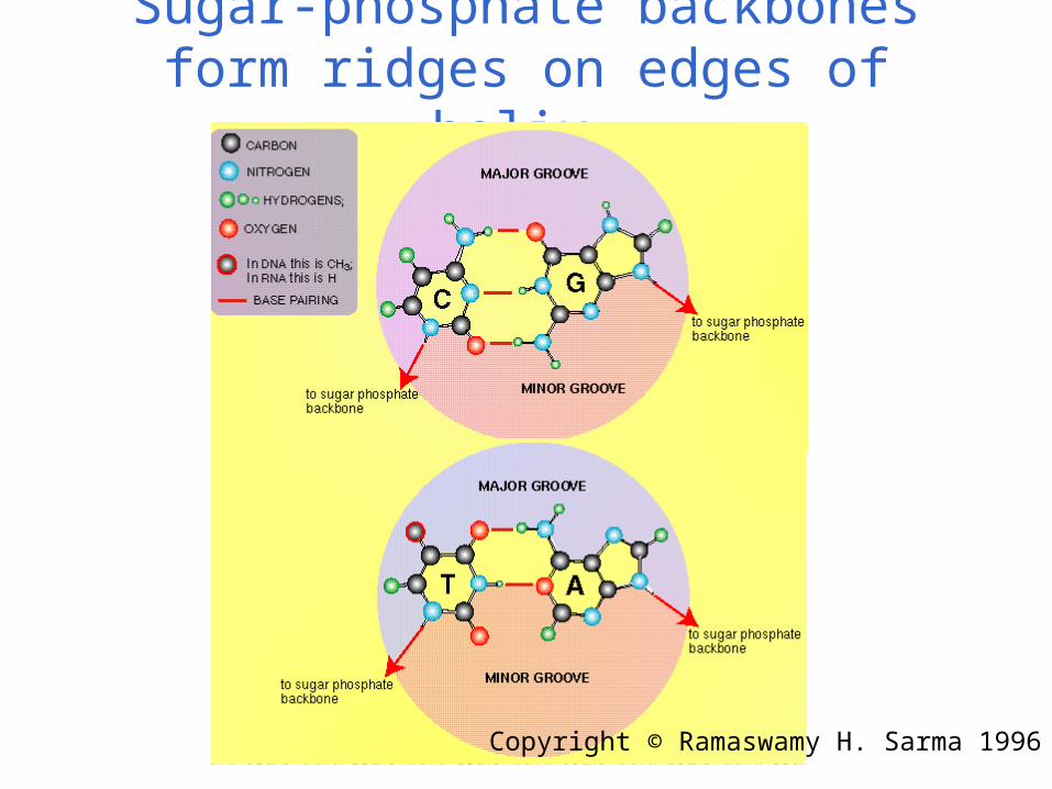
Sugar-phosphate backbones form ridges on edges of helix.

Copyright © Ramaswamy H. Sarma 1996

Classwork I.

1. Go to http://ndbserver.rutgers.edu/.

2. Select Crystal structure of B-DNA, resolution >=2 Angstroms.

3. Select Crystal structure of single-stranded RNA with mismatch base pairing with resolution >= 2 Angstroms.

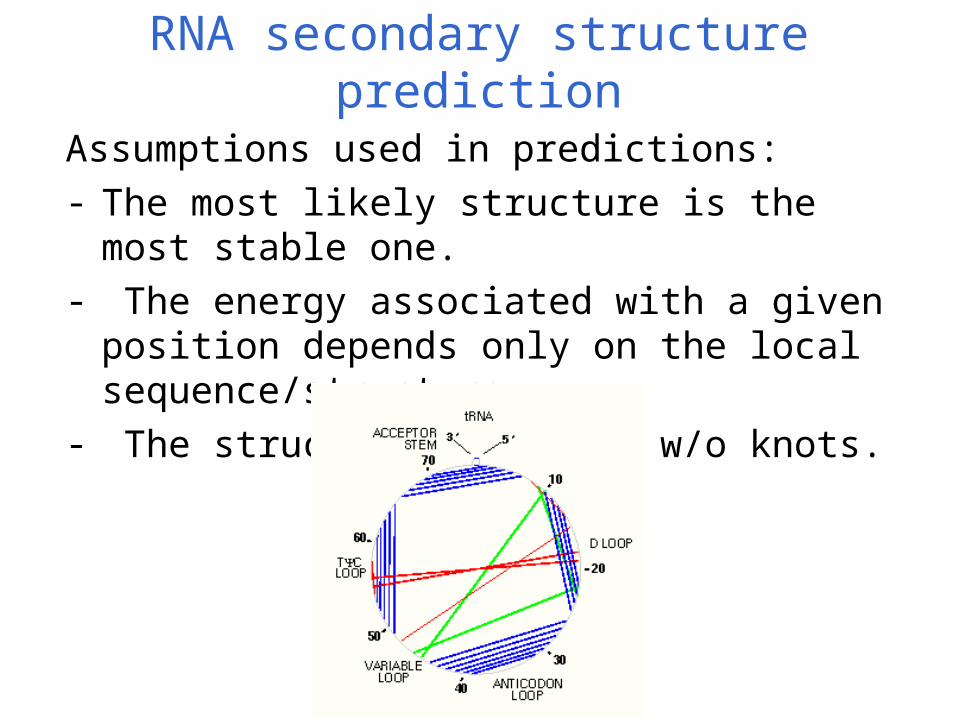
RNA secondary structure prediction

Assumptions used in predictions:- The most likely structure is the most stable one.- The energy associated with a given position

depends only on the local sequence/structure- The structure is formed w/o knots.

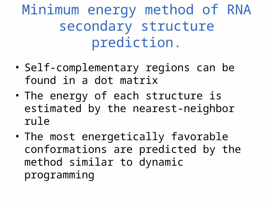
Minimum energy method of RNA secondary structure prediction.

• Self-complementary regions can be found in a dot matrix

• The energy of each structure is estimated by the nearest-neighbor rule

• The most energetically favorable conformations are predicted by the method similar to dynamic programming

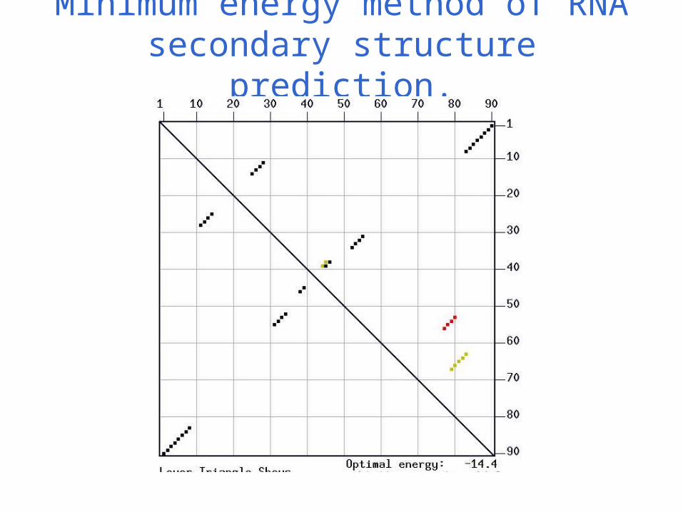
Minimum energy method of RNA secondary structure prediction.

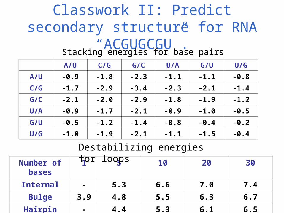
Classwork II: Predict secondary structure for RNA “ACGUGCGU”.

Stacking energies for base pairsA/U C/G G/C U/A G/U U/G

A/U -0.9 -1.8 -2.3 -1.1 -1.1 -0.8

C/G -1.7 -2.9 -3.4 -2.3 -2.1 -1.4

G/C -2.1 -2.0 -2.9 -1.8 -1.9 -1.2

U/A -0.9 -1.7 -2.1 -0.9 -1.0 -0.5

G/U -0.5 -1.2 -1.4 -0.8 -0.4 -0.2

U/G -1.0 -1.9 -2.1 -1.1 -1.5 -0.4

Number of bases

1 5 10 20 30

Internal - 5.3 6.6 7.0 7.4

Bulge 3.9 4.8 5.5 6.3 6.7

Hairpin - 4.4 5.3 6.1 6.5

Destabilizing energies for loops

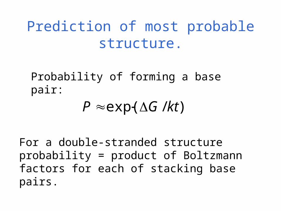
Prediction of most probable structure.

)/exp( ktGP

Probability of forming a base pair:

For a double-stranded structure probability = product of Boltzmann factors for each of stacking base pairs.

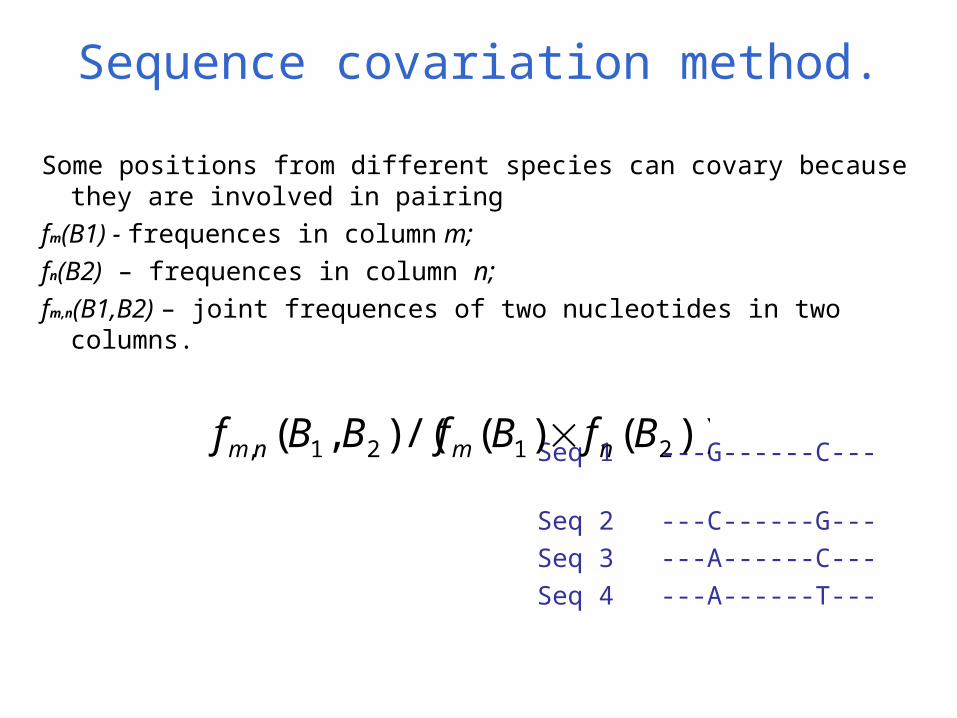
Sequence covariation method.

Some positions from different species can covary because they are involved in pairing

fm(B1) - frequences in column m;

fn(B2) – frequences in column n;

fm,n(B1,B2) – joint frequences of two nucleotides in two columns.

Seq 1 ---G------C---

Seq 2 ---C------G---

Seq 3 ---A------C---

Seq 4 ---A------T---

))()(/(),( 2121, BfBfBBf nmnm

Gene Prediction.

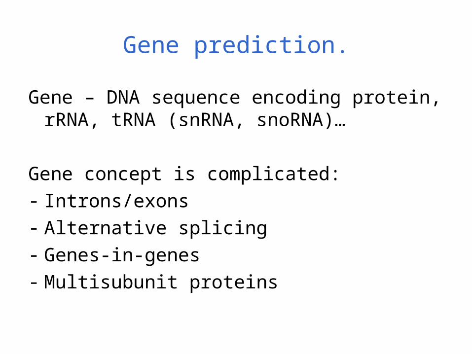
Gene prediction.

Gene – DNA sequence encoding protein, rRNA, tRNA (snRNA, snoRNA)…

Gene concept is complicated:

- Introns/exons

- Alternative splicing

- Genes-in-genes

- Multisubunit proteins

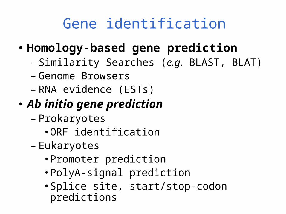
• Homology-based gene prediction– Similarity Searches (e.g. BLAST, BLAT)– Genome Browsers– RNA evidence (ESTs)

• Ab initio gene prediction– Prokaryotes

• ORF identification– Eukaryotes

• Promoter prediction• PolyA-signal prediction• Splice site, start/stop-codon predictions

Gene identification

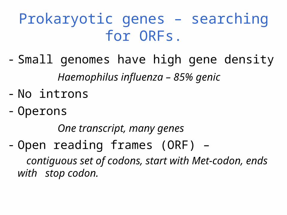
Prokaryotic genes – searching for ORFs.

- Small genomes have high gene density

Haemophilus influenza – 85% genic

- No introns

- Operons

One transcript, many genes

- Open reading frames (ORF) – contiguous set of codons, start with Met-codon,

ends with stop codon.

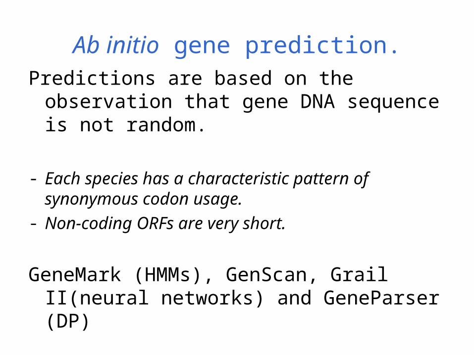
Ab initio gene prediction.

Predictions are based on the observation that gene DNA sequence is not random.

- Each species has a characteristic pattern of synonymous codon usage.

- Non-coding ORFs are very short.

GeneMark (HMMs), GenScan, Grail II(neural networks) and GeneParser (DP)

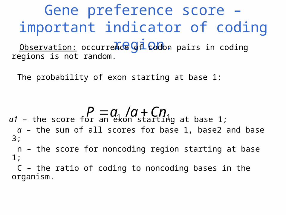
Gene preference score – important indicator of coding region.

Observation: occurrence of codon pairs in coding regions is not random.

The probability of exon starting at base 1:

a1 – the score for an exon starting at base 1; a – the sum of all scores for base 1, base2 and base 3; n – the score for noncoding region starting at base 1; C – the ratio of coding to noncoding bases in the organism.

11 / CnaaP

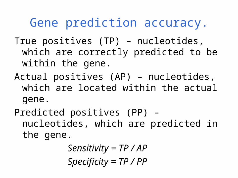
Gene prediction accuracy.

True positives (TP) – nucleotides, which are correctly predicted to be within the gene.

Actual positives (AP) – nucleotides, which are located within the actual gene.

Predicted positives (PP) – nucleotides, which are predicted in the gene.

Sensitivity = TP / AP

Specificity = TP / PP

Principles of protein structure and stability.

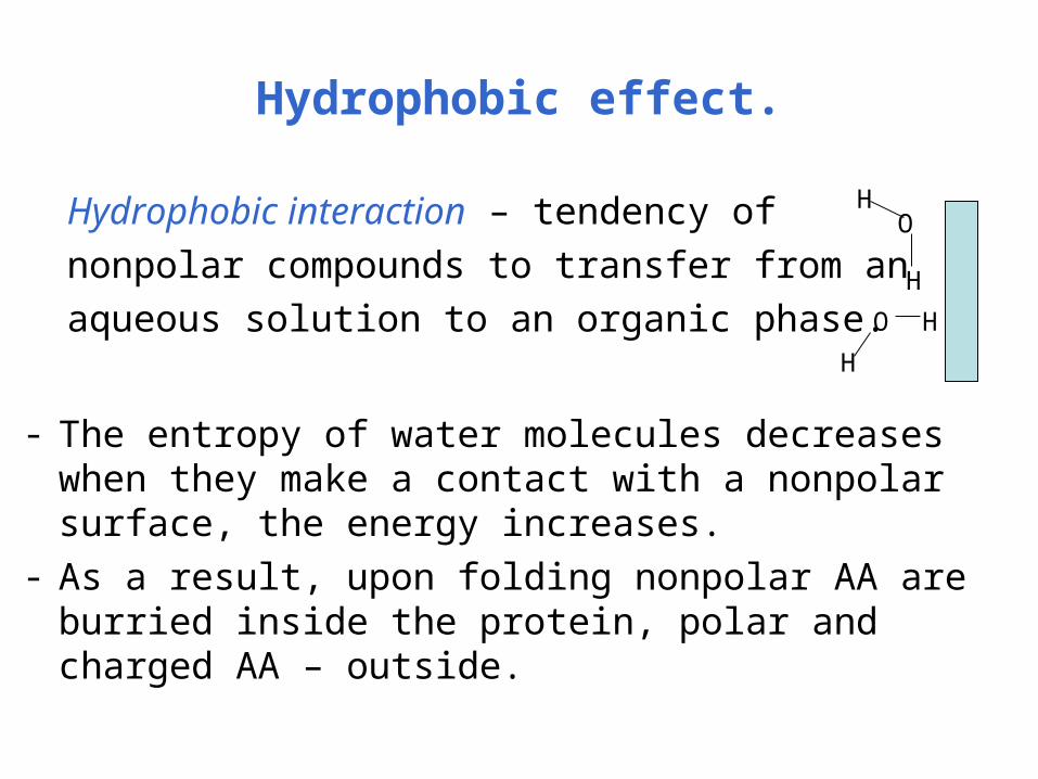
Hydrophobic effect.

Hydrophobic interaction – tendency of

nonpolar compounds to transfer from an

aqueous solution to an organic phase.

- The entropy of water molecules decreases when they

make a contact with a nonpolar surface, the energy increases.

- As a result, upon folding nonpolar AA are burried inside the protein, polar and charged AA – outside.

O

H

H

H

H

O

Summary:

- Hydrophobic effect is mostly responsible for making a compact globule. Final specific tertiary structure is formed by van der Waals interactions, HB, disulfide bonds.

- Secret of stability of native structures is not in the magnitude of the interactions but in their

cooperativity.

Protein secondary structure prediction.

Assumptions: • There should be a correlation between amino acid sequence

and secondary structure. Short aa sequence is more likely to form one type of SS than another.

• Local interactions determine SS. SS of a residues is determined by their neighbors (usually a sequence window of 13-17 residues is used).

Exceptions: short identical amino acid sequences can sometimes be found in different SS.

Accuracy: 65% - 75%, the highest accuracy – prediction of an α helix

Chou-Fasman method.

Analysis of frequences for all amino acids to be in different types of SS.

Ala, Glu, Leu and Met – strong predictors of alpha-helices,

Pro and Gly predict to break the helix.

)(/),(log(),( SfSafSaScore ii

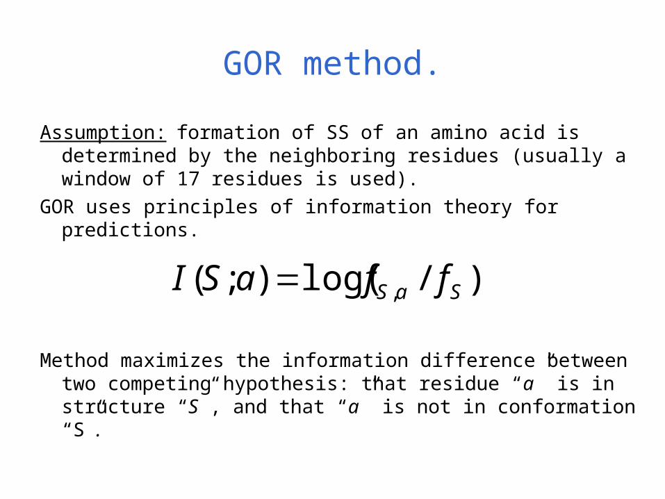
GOR method.

Assumption: formation of SS of an amino acid is determined by the neighboring residues (usually a window of 17 residues is used).

GOR uses principles of information theory for predictions.

Method maximizes the information difference between two competing hypothesis: that residue “a” is in structure “S”, and that “a” is not in conformation “S”.

)/log();( , SaS ffaSI

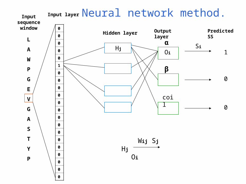
Neural network method.

L

A

W

P

G

E

V

G

A

S

T

Y

P

0

0

0

0

0

1

0

0

0

0

0

0

0

0

0

0

0

0

0

0

0

HjOi

α

β

coil

1

0

0

Si

Hj Oi

Wij Sj

Input sequence window

Input layer

Hidden layer Output layer Predicted SS

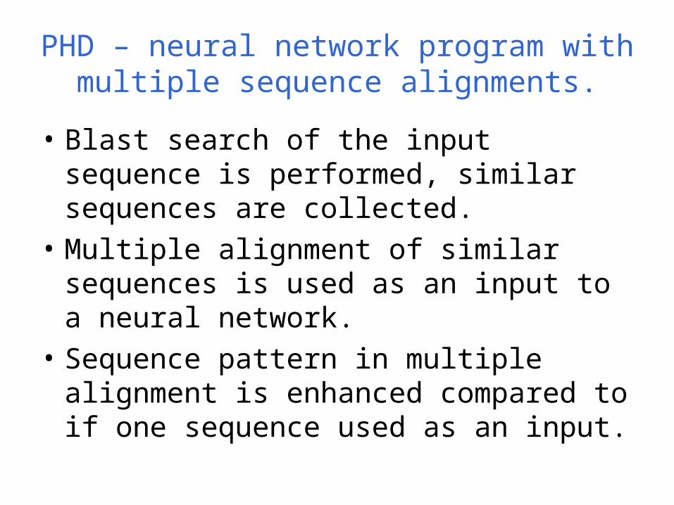
PHD – neural network program with multiple sequence alignments.

• Blast search of the input sequence is performed, similar sequences are collected.

• Multiple alignment of similar sequences is used as an input to a neural network.

• Sequence pattern in multiple alignment is enhanced compared to if one sequence used as an input.

Classwork

• Go to http://ncbi.nlm.nih.gov, search for protein “flavodoxin” in Entrez, retrieve its amino acid sequence.

• Go to http://cubic.bioc.columbia.edu/predictprotein and run PHD on the sequence.

The Conserved Domain Architecture Retrieval Tool (CDART).

• Performs similarity searches of the NCBI Entrez Protein Database based on domain architecture, defined as the sequential order of conserved domains in proteins.

• The algorithm finds protein similarities across significant evolutionary distances using sensitive protein domain profiles. Proteins similar to a query protein are grouped and scored by architecture.

Fold recognition.

Unsolved problem: direct prediction of protein structure from the physico-chemical principles.

Solved problem: to recognize, which of known folds are similar to the fold of unknown protein.

Fold recognition is based on observations/assumptions:- The overall number of different protein folds is limited

(1000-3000 folds)

- The native protein structure is in its ground state (minimum energy)

Protein structure prediction.

Prediction of three-dimensional structure from its protein sequence. Different approaches:

- Homology modeling (predicted structure has a very close homolog in the structure database).

- Fold recognition (predicted structure has an existing fold).

- Ab initio prediction (predicted structure has a new fold).

Steps of homology modeling.

1. Template recognition & initial alignment.

2. Backbone generation.

3. Loop modeling.

4. Side-chain modeling.

5. Model optimization.

6. Model validation.

Classwork I: Homology modeling.

- Go to NCBI Entrez, search for gi461699

- Do Blast search against PDB

- Do CD-search.

Fold recognition.

Goal: to find in PDB a fold which best matches a given sequence.

Since similarity between target and the closest to it template is not high, sequence-sequence alignment methods fail to find a closest match.

Solution: threading – sequence-structure alignment method.

Threading – method for structure prediction.

Sequence-structure alignment, target sequence is compared to all structural templates from the database.

Requires:- Alignment method (dynamic programing, Monte

Carlo,…)- Scoring function, which yields relative score for

each alternative alignment

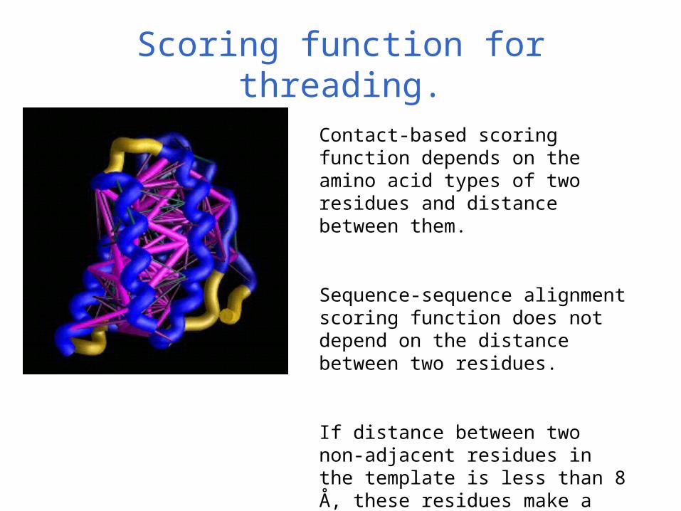
Scoring function for threading.

Contact-based scoring function depends on the amino acid types of two residues and distance between them.

Sequence-sequence alignment scoring function does not depend on the distance between two residues.

If distance between two non-adjacent residues in the template is less than 8 Å, these residues make a contact.

Mechanisms of evolution.

- Evolution is caused by mutations of genes.

- Mutations spread through the population via genetic drift and/or natural selection.

- If mutant gene produces an advantage (new morphological character), this feature will be

inherited by all descendant species.

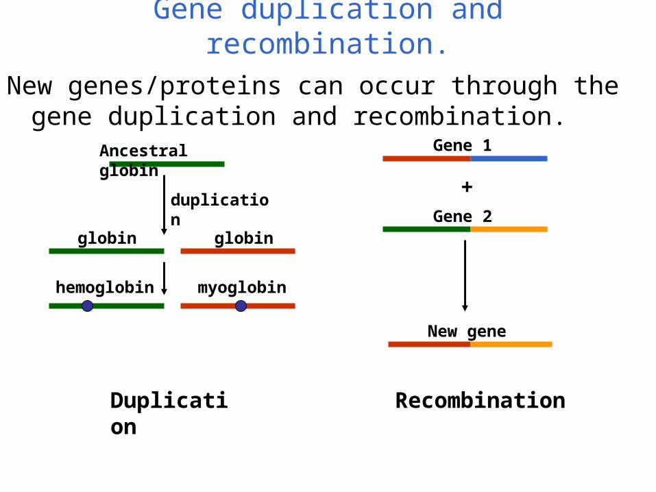
Gene duplication and recombination.

New genes/proteins can occur through the gene duplication and recombination.

Ancestral globin

duplication

globin globin

hemoglobin myoglobin

Duplication

+

Gene 1

Gene 2

New gene

Recombination

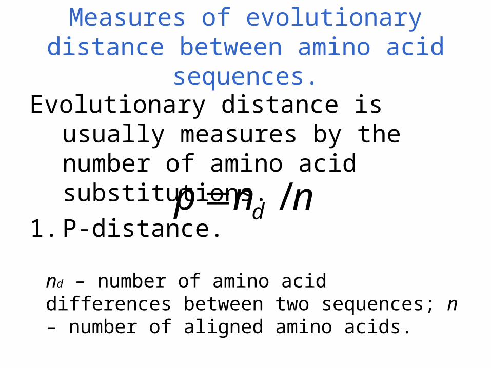
Measures of evolutionary distance between amino acid sequences.

Evolutionary distance is usually measures by the number of amino acid substitutions.

1. P-distance.

nnp d /

nd – number of amino acid differences between two sequences; n – number of aligned amino acids.

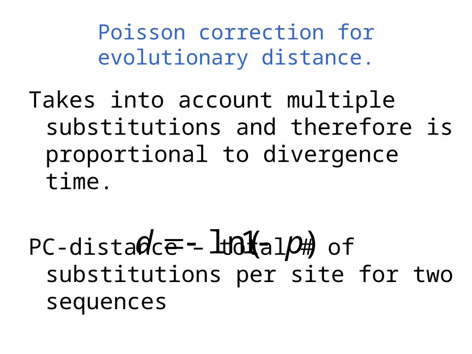
Poisson correction for evolutionary distance.

Takes into account multiple substitutions and therefore is proportional to divergence time.

PC-distance – total # of substitutions per site for two sequences )1ln( pd

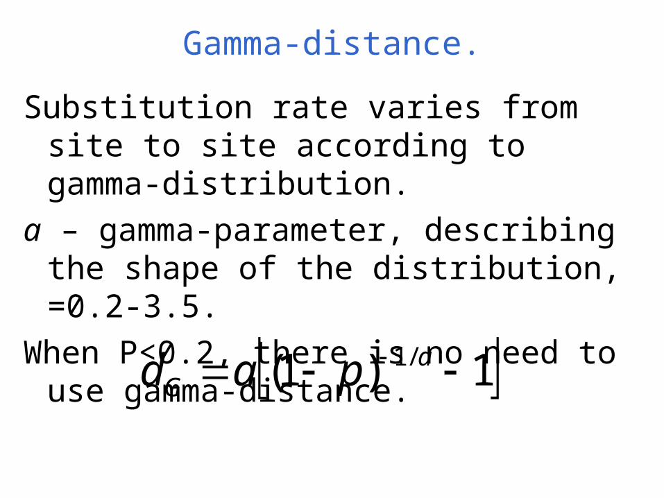
Gamma-distance.

Substitution rate varies from site to site according to gamma-distribution.

a – gamma-parameter, describing the shape of the distribution, =0.2-3.5.

When P<0.2, there is no need to use gamma-distance.

1)1( /1 aG pad

Another method to estimate evolutionary distances: amino acid substitution matrices.

Substitutions occur more often between amino acids of similar properties.

Dayhoff (1978) derived first matrices from multiple alignments of close homologs.

The number of aa substitutions is measured in terms of accepted point mutations (PAM) – one aa substitution per 100 sites.

Dayhoff-distance can be approximated by gamma-distance with a=2.25.

The concept of evolutionary trees.

- Trees show relationships between organisms.

- Trees consist of nodes and branches, topology - branching pattern.

- The length of each branch represents the number of substitutions occurred between two nodes. If rate of evolution is constant, branches will have the same length (molecular clock hypothesis).

- Trees can be binary or bifurcating.- Trees can be rooted and unrooted. The root is placed by

including a taxon which is known to branch off earlier than others.

Accuracies of phylogenetic trees.

Two types of errors:- Topological error- Branch length error

Bootstrap test:

Resampling of alignment columns with replacement; recalculating the tree; counting how many times this topology occurred – “bootstrap confidence value”. If it is >0.95 – reliable topology/interior branch.

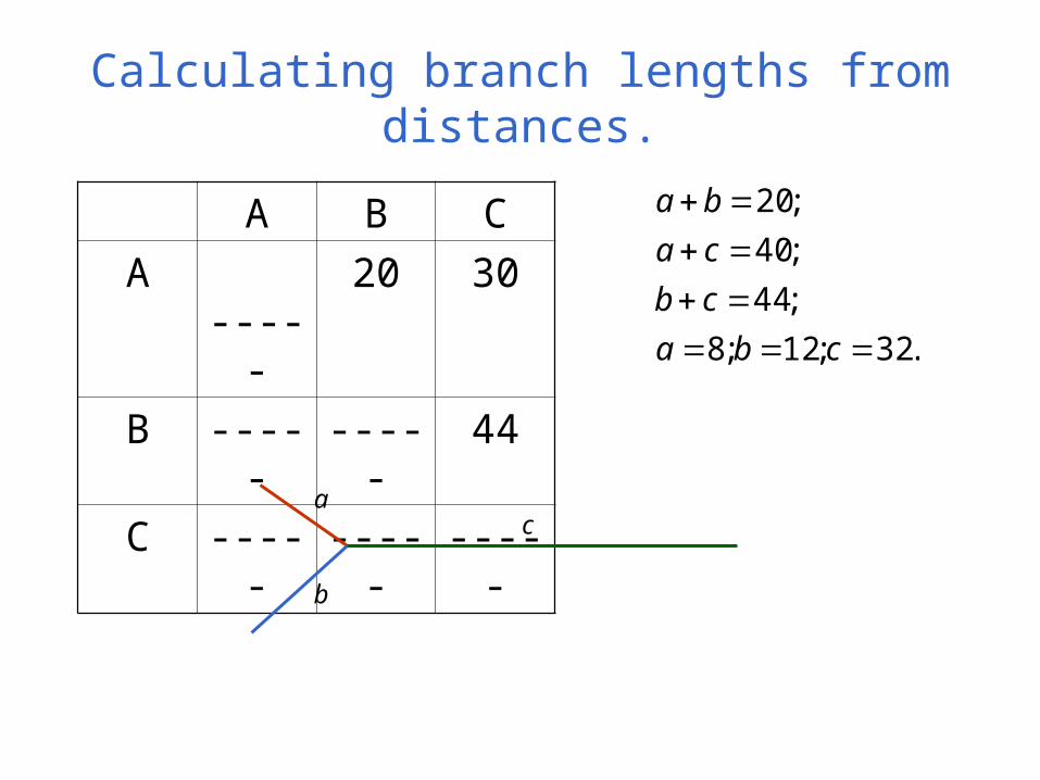
Calculating branch lengths from distances.

A B C

A ----- 20 30

B ----- ----- 44

C ----- ----- -----.32;12;8

;44

;40

;20

cba

cb

ca

ba

a

b

c

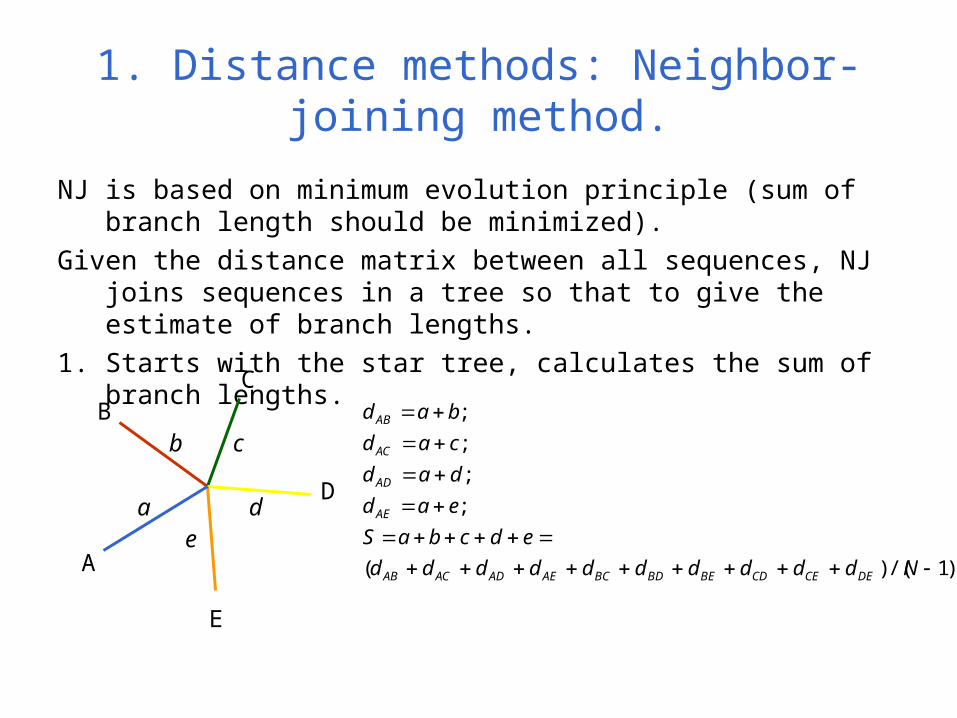
1. Distance methods: Neighbor-joining method.

NJ is based on minimum evolution principle (sum of branch length should be minimized).

Given the distance matrix between all sequences, NJ joins sequences in a tree so that to give the estimate of branch lengths.

1. Starts with the star tree, calculates the sum of branch lengths.

A

BC

D

E

a

b c

de

)1/()(

;

;

;

;

Ndddddddddd

edcbaS

ead

dad

cad

bad

DECECDBEBDBCAEADACAB

AE

AD

AC

AB

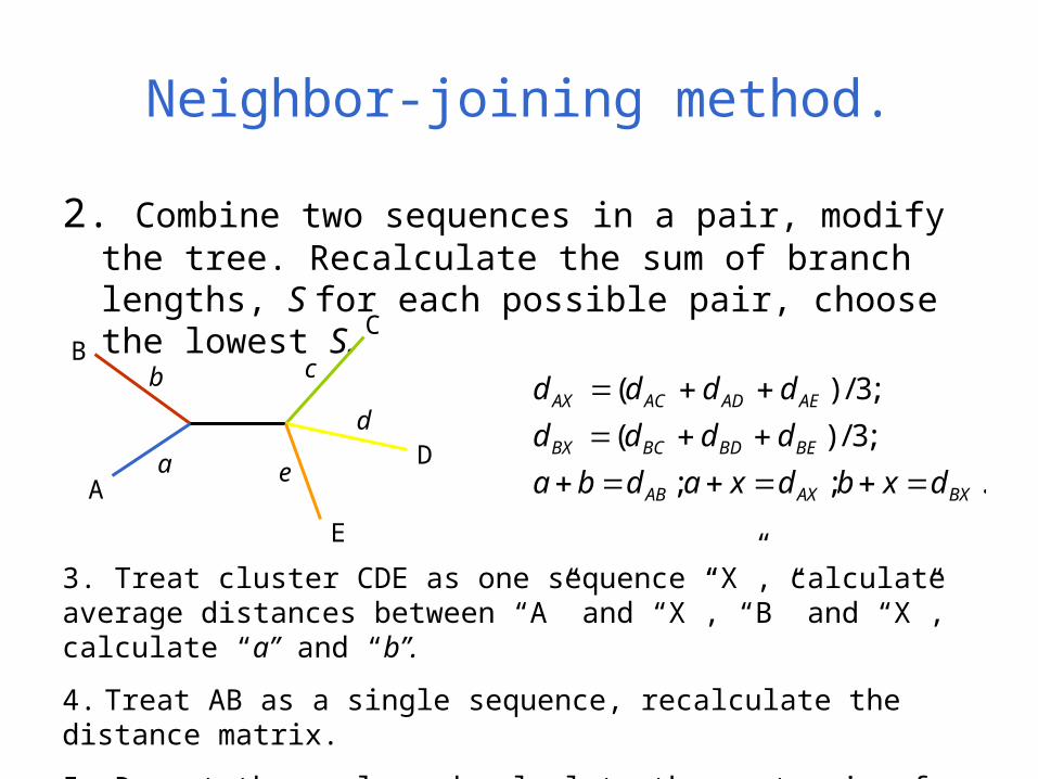
Neighbor-joining method.

2. Combine two sequences in a pair, modify the tree. Recalculate the sum of branch lengths, S for each possible pair, choose the lowest S.

A

BC

D

E

a

b c

d

e .;;

;3/)(

;3/)(

BXAXAB

BEBDBCBX

AEADACAX

dxbdxadba

dddd

dddd

3. Treat cluster CDE as one sequence “X”, calculate average distances between “A” and “X”, “B” and “X”, calculate “a” and “b”.

4. Treat AB as a single sequence, recalculate the distance matrix.

5. Repeat the cycle and calculate the next pair of branch lengths.

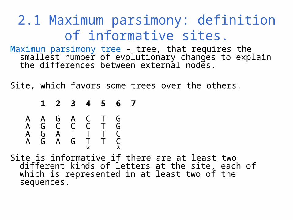
2.1 Maximum parsimony: definition of informative sites.

Maximum parsimony tree – tree, that requires the smallest number of evolutionary changes to explain the differences between external nodes.

Site, which favors some trees over the others.

1 2 3 4 5 6 7

A A G A C T G A G C C C T G A G A T T T C A G A G T T C * * Site is informative if there are at least two different kinds of letters

at the site, each of which is represented in at least two of the sequences.

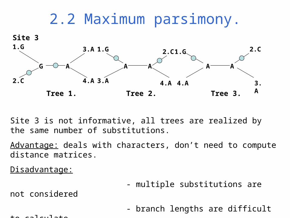
2.2 Maximum parsimony.

1.G

2.C

G A

3.A

4.A

A

1.G

3.A

A

2.C

4.A

1.G

4.A

A A

2.C

3.A

Tree 1. Tree 2. Tree 3.

Site 3

Site 3 is not informative, all trees are realized by the same number of substitutions.

Advantage: deals with characters, don’t need to compute distance matrices.

Disadvantage:

- multiple substitutions are not considered

- branch lengths are difficult to calculate

- slow

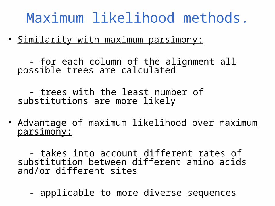
Maximum likelihood methods.

• Similarity with maximum parsimony:

- for each column of the alignment all possible trees are calculated

- trees with the least number of substitutions are more likely

• Advantage of maximum likelihood over maximum parsimony:

- takes into account different rates of substitution between different amino acids and/or different sites

- applicable to more diverse sequences

Molecular clock.

• First observation: rates of amino acid substitutions in hemoglobin and cytochrome c are ~ the same among different mammalian lineages.

• Molecular clock hypothesis: rate of evolution is ~ constant over time in different lineages; proteins evolve at constant rates.

• This hypothesis is used in estimating divergence times and reconstruction of phylogenetic trees.

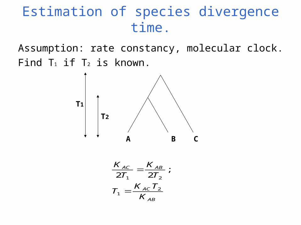
Estimation of species divergence time.

Assumption: rate constancy, molecular clock.

Find T1 if T2 is known.

A B C

T1

T2

AB

AC

ABAC

K

TKT

T

K

T

K

21

21

;22

Neutral theory of evolution.

• Kimura in 1968: majority of molecular changes in evolution are due to the random fixation of neutral mutations (do not effect the fitness of organism.

• As a consequence the random genetic drift occurs.

• Value of selective advantage of mutation should be stronger than effect of random drift.

Genome analysis.

Genome – the sum of genes and intergenic sequences of a haploid cell.

Analysis of gene order (synteny).

Genes with a related function are frequently clustered on the chromosome.

Ex: E.coli genes responsible for synthesis of Trp are clustered and order is conserved between different bacterial species.

Operon: set of genes transcribed simultaneously with the same direction of transcription

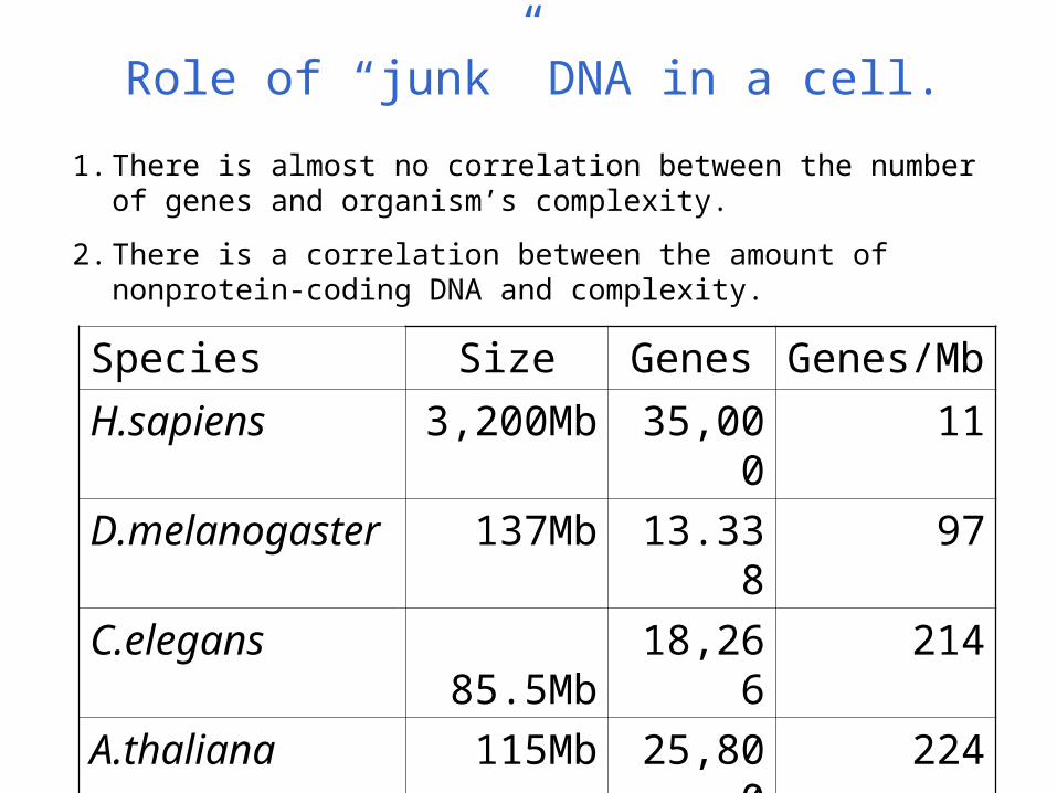
Role of “junk” DNA in a cell.

Species Size Genes Genes/Mb

H.sapiens 3,200Mb 35,000 11

D.melanogaster 137Mb 13.338 97

C.elegans 85.5Mb 18,266 214

A.thaliana 115Mb 25,800 224

S.cerevisiae 15Mb 6,144 410

E.coli 4.6Mb

4,300 934

1. There is almost no correlation between the number of genes and organism’s complexity.

2. There is a correlation between the amount of nonprotein-coding DNA and complexity.

Regulatory role of non-coding regions.

- “Micro-RNAs” control timing of processes in development and apoptosis.

- Intron’s RNAs inform about the transcription of a particular gene.

- Alternative splicing can be regulated by non-coding regions.

- Non-coding regions can be very well conserved between the species and many genetic deseases have been linked to variations/mutations in non-coding regions.

Systems biology.

• Integrative approach to study the relationships and interactions between various parts of a complex system.

Goal: to develop a model of interacting components for the whole system.

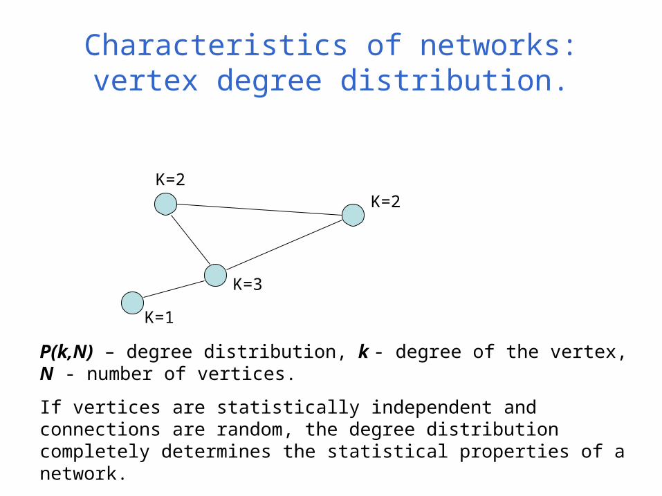
Characteristics of networks: vertex degree distribution.

K=2K=2

K=3

K=1

P(k,N) – degree distribution, k - degree of the vertex, N - number of vertices.

If vertices are statistically independent and connections are random, the degree distribution completely determines the statistical properties of a network.

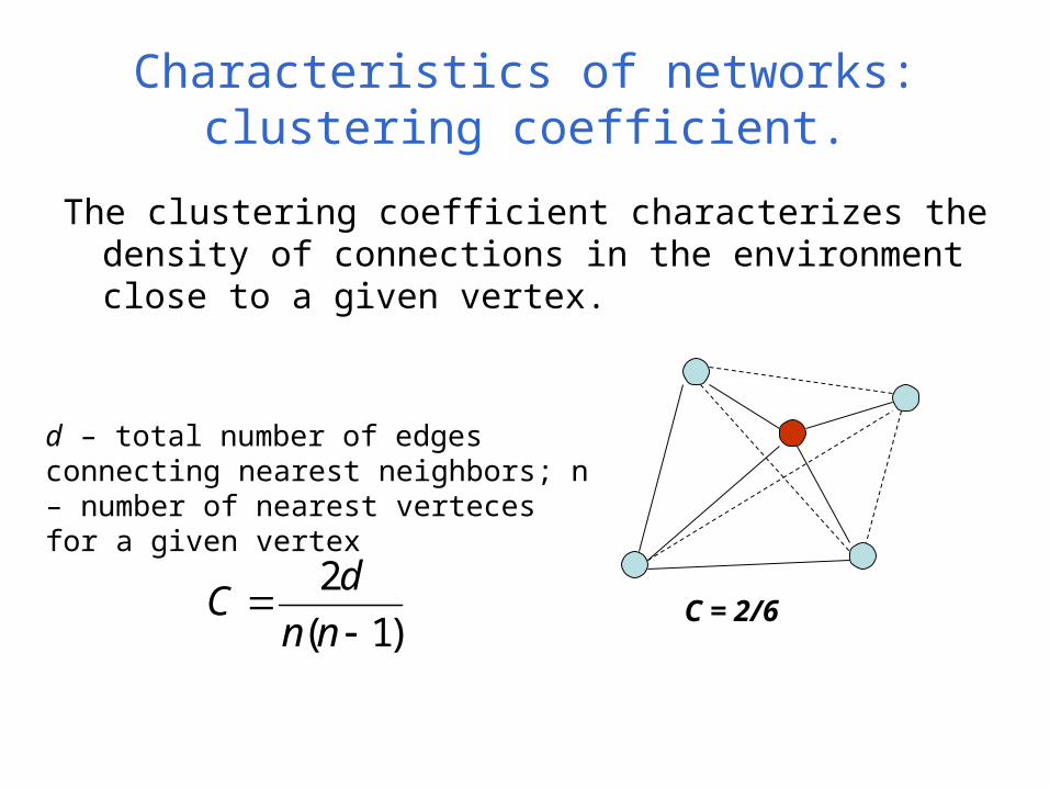
Characteristics of networks: clustering coefficient.

The clustering coefficient characterizes the density of connections in the environment close to a given vertex.

)1(

2

nn

dC

d – total number of edges connecting nearest neighbors; n – number of nearest verteces for a given vertex

C = 2/6

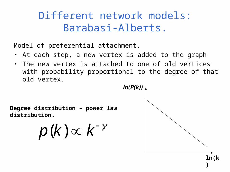
Different network models: Barabasi-Alberts.

Model of preferential attachment.• At each step, a new vertex is added to the graph• The new vertex is attached to one of old vertices with probability

proportional to the degree of that old vertex.

ln(P(k))

ln(k)

kkp )(

Degree distribution – power law distribution.

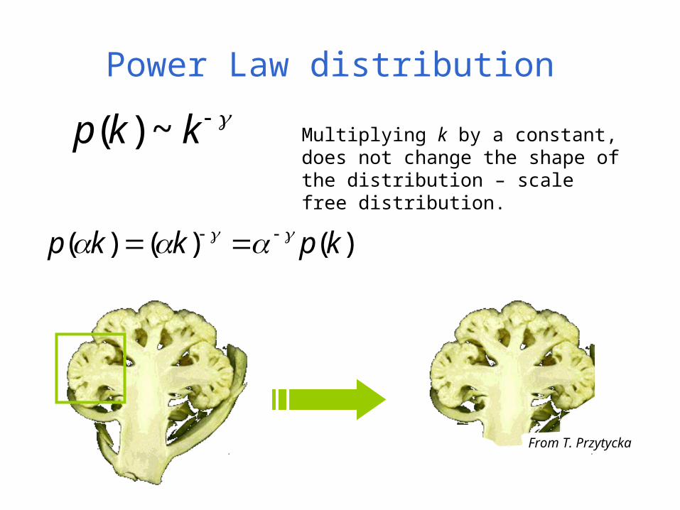
Power Law distribution

kkp ~)(

)()()( kpkkp

Multiplying k by a constant, does not change the shape of the distribution – scale free distribution.

From T. Przytycka

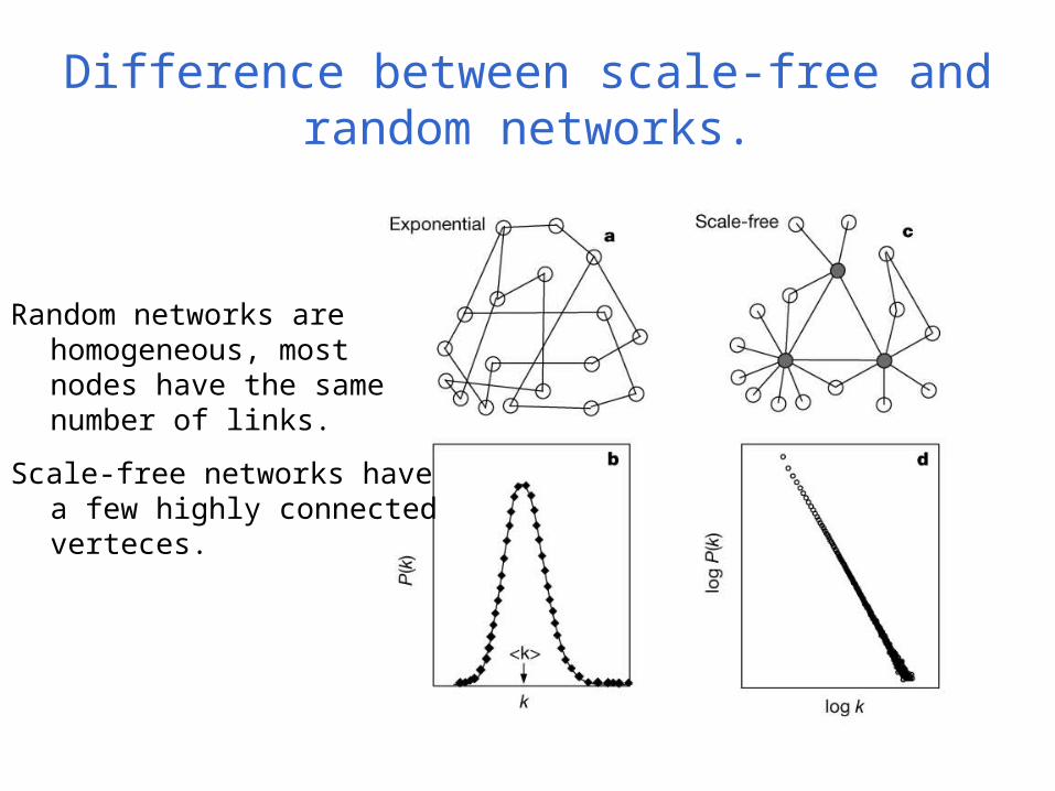
Difference between scale-free and random networks.

Random networks are homogeneous, most nodes have the same number of links.

Scale-free networks have a few highly connected verteces.