A Survey on Modeling Economic GrowthWith Special Interest on Natural Resource Use

Frauke Voosholz∗

Corrected Draft September 2014

CAWM Discussion Paper No. 69

Abstract

The purpose of this paper is to survey the contributions to economic growththeory. We focus on the basic models and literature that link resource economicand economic growth, in order to reveal the main differences on how the differentaspects are incorporated into growth models. As economic science is not a hardscience, all economic activities must always be considered against the backgroundof the economy, the political and social institutions, and technical capabilities atthat time (as already mentioned by Solow (1985), p. 328). That is why many ofthe first growth models, fitted to contemporary state, when they were developed,are not transferable to remote periods. Furthermore, natural resources as inputfactors, which influence economic growth, were neglected for a long time, whereastoday they are one of the most discussed factors influencing economic growth.

JEL classification: O13, O41, O40, Q20, Q32

Keywords: economic growth, growth theory, historical overview, renew-able resources, non-renewable resources

∗Dipl. Volksw. Frauke Voosholz, University of Muenster, Institute of Spacial and Housing Economics,Am Stadtgraben 9, 48143 Muenster / Germany, Tel. +49-251-83-22979, f voos01@wiwi.uni-muenster.de

1

1 Why is Growth so Important?

There are 215 countries in the world, whose GDPs (gross domestic product) are growing

at different rates. Even small differences in the growth rates lead to enormous differences

in real terms, if running with the same start value (after 100 years, a growth rate of 0.7

percent leads to twice the starting GDP, a rate of 1.7 percent leads to an increment of 5.4

times). Some countries, like Qatar and Paraguay, are growing rapidly with an inflation

adjusted increase of the GDP of about 15 percent a year, some are not growing at all,

others, like Puerto Rico, Anguilla and San Marino, are even dwindling by more than

five percent a year (cf. CIA - Central Intelligence Agency (2010)). The GDP does not

represent in full the real state of the individual welfare of people living in those countries,

but it is one of the best ways to compare countries quantitatively. The income per person

is a useful index, highly correlated to quality of life. According to the scientific approach

it may be reasonable to add further indicators, e.g. public welfare or working lifetime.

But why do growth rates differ ever so much? Every country has a different starting

point. The supply of labor, the stock of resources, capital and human capital, the level of

infrastructure, and the climate conditions are some of the main aspects influencing the

development of countries. Further aspects affecting the process of growth are the political

and institutional environment, the volume of international trade and the current GDP.

Growth models try to capture these facts to show the relationships and the development

of the variables. They try to reveal how decisions made by economic agents, the value

of the variables in the past, present and future, as well as specific implications affect the

growth rates.

Studies in economic growth want to make a contribution to solutions on economic-

political problems. So it is important to keep in mind the implications, the adequacy to

the purpose and the suitability of instruments. Even similar problems often need specific

methods, and even the same problem cannot be solved in the same way in each country

because in a specific situation there are a lot of interdependencies between different

political issues.

Generally in political and public discussions only a growth rate above two percent is

regarded as sufficient; in some countries a satisfying growth rate is even claimed by law,

e.g. Germany (cf. Bundesministerium der Justiz (1967) paragraph 1). This is accounted

for by the general definition of growth. Growth is understood as a sustained extension

of good-production, so that the average household may use more products and achieve

a greater level of satisfaction and happiness. The importance of a growth rate not only

greater than zero, but even larger, is determined by the fact that the growth rate must

be higher than the inflation rate to achieve this goal.

Alongside of the direct goal of economic growth, there are more indirect goals of eco-

2

nomic policies, seeing economic growth only as a means to an end (cf. Meyer et al. (1998)

pp. 1-2). While technical improvement leads to higher average labor productivity, the

employment rate can only be kept constant or be raised if more goods can be distributed.

Another goal, a fairer income distribution, is usually more easily achievable if there is

additional income as basis for the reallocation.

In addition, growth has to be evaluated. It influences many fields that often are not di-

rectly included in economic questions. It is relevant which impact it has on the individual

utility and on the society. The positive effects have to be balanced with the cost of growth,

like, for example, environmental destruction or less leisure time. Keeping in mind that

we are dealing with production functions, which include the development of resources,

it must be guaranteed that not only one generation benefits from economic growth, but

that it is long lasting and sustainable. Especially, the exhaustion of non-renewable re-

sources must be taken into account. Here technical progress and a substitution progress

are important to keep on the economy growing.

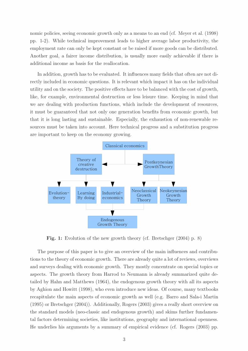
Fig. 1: Evolution of the new growth theory (cf. Bretschger (2004) p. 8)

The purpose of this paper is to give an overview of the main influences and contribu-

tions to the theory of economic growth. There are already quite a lot of reviews, overviews

and surveys dealing with economic growth. They mostly concentrate on special topics or

aspects. The growth theory from Harrod to Neumann is already summarized quite de-

tailed by Hahn and Matthews (1964), the endogenous growth theory with all its aspects

by Aghion and Howitt (1998), who even introduce new ideas. Of course, many textbooks

recapitulate the main aspects of economic growth as well (e.g. Barro and Sala-i Martin

(1995) or Bretschger (2004)). Additionally, Rogers (2003) gives a really short overview on

the standard models (neo-classic and endogenous growth) and skims further fundamen-

tal factors determining societies, like institutions, geography and international openness.

He underlies his arguments by a summary of empirical evidence (cf. Rogers (2003) pp.

3

122-128). Rostow (1959) looks on economic growth from a different perspecitve. In his

review he concentrates on the stages of growth in a describing non-theoretical context,

depending on the different stages of the development of societies (cf. Rostow (1959) p.

1).

The main aim of the paper is to show how the different schools of economic build

on one another and influence todays dealing with economic growth and its presentation

in theoretical literature (see Fig. 1). This survey is arranged in five main sections

and proceeds as follows. At first, a short historical overview of the theory of growth

is given. We discuss the historical background of growth theory, followed by the main

basic theories of economic growth. In a further section the fundamentals of endogenous

growth theory are discussed. Section five introduces factors influencing economic growth,

thereby concentrating on resources and the differences in research design. We conclude

by giving an outlook on further research requirement.

2 Some Background of Growth Models

We start with the classical economists of the 18th and 19th century, who made

important discoveries in their grand theories, building the basis of further

research. Influenced by this, Schumpeter made a first step to a new field

of research by his theory of creative destruction, and coevally the idea of

accelerators and multiplicators was introduced.

2.1 Fundamentals of Growth Theory

The Tableau economique, educed by Francois Quesney (1694-1774), can be interpreted

as first growth model (later translated edition, see Quesney (1965)). Quesnay states that

only land is net-productive; the land lords will invest all their income (production Y less

consumption C). Assuming constant prices, the amount of goods produced depends only

on the consumption rate c, and therefore, determines whether production grows, declines

or is stationary (formally written g = 0.5 (c− 0.5) − 2/3 (c− 0.5)2, see Eltis (1975) p.

333).

The classical economics, replacing the physiocratic body of thought, included in their

grand theories many aspects which were later used as science base of the first attempts

to describe long-run economic growth in more detail. The main aspects of these grand

theories relevant for economic growth will be described shortly in the style of current

formal models. As a basis of the classical economics Adam Smith’s “An Inquiry into

the Nature and Causes of the Wealth of Nations” (Smith (1776)) can be seen. Most

4

principals are mentioned there, even though there are still many discrepancies between

the different elements of his book (cf. Stavenhagen (1969) pp. 52 ff.).

Adam Smith (1723-1790) concentrates mainly on the definition of wealth, how it

arises and why it grows. In contrast to the physiocrates, he points out that the labor

performed by the nation is the source of wealth and not the agricultural, primary pro-

duction. The efficiency of labor depends on the division of labor, and the division of

labor needs functioning markets. Smith’s production function may read roughly like this:

Y = Y (K,L, T ) where T is usable land with T ≤ Tmax (see Meyer et al. (1998) pp. 52 et

seqq.). As long as there is a lot of usable land uncultivated, the enlargement of the pro-

duction is determined by the capital accumulation and population growth. If at the same

time the division of labor is growing, the returns to scale are growing, too. The closer

the economy reaches the limit of population growth (Nmax), depending on the natural

endowment of the economy (land, climate, etc.), and has reached a high level of labor

division, the more the returns to scale decrease. In the long-run, economies, following

Smith, reach a steady state.

In the different editions of “An Essay on the Principle of Population” Thomas

Robert Malthus (1766-1834) mainly develops a population theory, where the popu-

lation growth (geometric series nt+1 = nt · 2) is always stronger than the growth of food

production (arithmetic series yt+1 = yt + 1) (see Malthus (1798), chapter 2). Therefore,

there is a limit to population growth, even under the condition of technological progress.

Savings, and consequently, waiver of consumption were the determining factors for eco-

nomic growth. But there was the risk of a lack of demand, which would induce a negative

cycle. In summary, Malthus puts forward the assumption that there is a stationary final

state without growth, when the optimal size of population is reached. But this state

would only be achieved after a long period of time.

A further important classical economist is David Ricardo (1772-1823). In his stud-

ies, compiled in “On the Principles of Political Economy and Taxation” (Ricardo (1821)),

he mainly dealt with the allocation of income between capital, labor and land (cf. Eltis

(1989) p. 202). As long as only fertile soils are used, the tenants achieve a higher rent (for

capital). Those profits are normally invested in production, more land can be cultivated,

more workforce employed. At some point in time, the less fertile pieces of land have to

be used by the tenants to enlarge the production. At this time, the tenants’ profits are

reduced because they have to pay a higher rent for the best soils to the landowners. As

long as they receive a bit more than the minimum rent, the tenants will invest, and it is

possible that the population of the economy grows or that the workers can enlarge their

demand for goods. If the minimum rent is reached, the economy reaches a stationary

state. The price of goods is controlled by the amount of labor used for the production.

To overcome the stationary state, Ricardo advocated international trade, so that every

5

economy could specialize in the product where they have an advantage regarding the

costs of production in comparison to the other countries (cf. Heertje and Wenzel (2008)

p. 51). The wealth of the economies can be increased in this way.

In 1848 John Stuart Mill (1806-1873) tried to summarize the current state of the

economic theory in his publication “Principles of Political Economy”. He subdivides the

economic theory in five categories “Production”, “Distribution”, “Exchange”, “Influence

of the progress of society on Production and Distribution”, and “Influence of Government”

(Mill (1848)). Until today his structure is important in economic research. At the same

time he developed the ideas of earlier acting economists and introduced new modifications.

He tried to keep in touch with the reality and the consequences on political proceedings,

by trying to introduce a reform party (cf. Marchi (1989) p. 272). He kept the idea of

a stationary final state, welcomed by him because it may lead to a fair and cultivated

social existence (cf. Holub (2010) p. 233). A further important aspect of Mill’s research

was that he concentrated on the maximization of utility and fortune, in contrast to profit

maximization (cf. ibidem pp. 229-230).

Friedrich List (1798-1846) encourages this idea as well. He assumed that each

nation had to develop itself, using investments and technological progress, to reach a

higher productivity. Prohibitive taxes may be used by nations which have not reached

the maximum level of industrialization yet (cf. List (1841) p. 18).

An important contribution is the fact that factor aggregation, associated with in-

creasing or diminishing returns to scale, which is crucial to many growth models, was

introduced by Alfred Marshall (1842-1924) and introduced into growth economy (see

Romer (1994) p. 14). He summarizes that “every increase of wealth and every increase

in the numbers and intelligence of the people increased the facilities for a highly devel-

oped industrial organization, which in its turn adds much to the collective efficiency of

capital and labor” (Marshall (1980) book 4, chap. 13, paragraph 1).

In total, one could say that these economists were more interested in development

in the long-run than in short-term changes. They mostly assumed that there is a sta-

tionary limit to which all initially growing economies convert, accounted for by different

mechanisms.

2.2 From the Theory of Long-period Equilibrium to the Theory

of Growth

In contrast to the former theories, Joseph Alois Schumpeter (1883-1950) sees inno-

vations as the main driving force for economic growth. A constant evolution and mod-

ification of products and production processes, new customers and suppliers, and even

6

changes in the political settings lead to new market structures and temporary monopoles

(Schumpeter (1934)). At the same time old ideas become inefficient, and the economic

cycle, the possible finale state and the equilibrium are changed. Schumpeter had in mind

innovations like e.g. the steam-engine or the railroad system, which occur as episodes.

Using the idea of Albert Aftalion (1874-1956), the accelerator principle was devel-

oped by John Bates Clark (1847-1938) (cf. first published in French 1913, Aftalion

(1927) and Clark (1917)). It states that investment depends on consumption and a con-

stant accelerator c, that is why a change in consumption leads to an over-proportional

change in investments, formally I = c · dCdt

with c > 1, which leads to economic growth

(cf. Clark (1917) p. 223).

In contrast to J. B. Clark, John Maynard Keynes (1883-1946) states that the

amount of investments is independently set, and the total income is given by Y = C + I.

The national income may either be consumed C or saved for investments S, consequently

consumption is a function of the total income. If the marginal propensity to consume c′ is

constant, the multiplier results from dYdt

= 1

1−c′·dIdt; a change in the amount of investments

leads to a change of the total income, subject to the multiplier 1

1−c′(Keynes (1936)). If

the equilibrium of S = I is disturbed, additional national investments have to be made

to restore the equilibrium. However, his theory does not lead to suggestions concerning

long-run growth, rather to guidance in different phases of the economic cycle (cf. Murad

(1962) p. 57).

Karl Marx (1818-1883) uses theoretical considerations, concerning two different eco-

nomic sectors. Equilibrium is reached if and only if both sectors grow at the same rate.

Formally the growth rate g is defined by the ration of savings and investment rate s to

the capital coefficient z, where z is determined by the ratio of fixed and variable capital

to wages and the income of the capitalists. If s and z are constant, continuous balanced

growth is possible (see Marx (1962) with an example in chapter 21, section 3, III). Origi-

nally, Marx states that the composition of capital z grows because of the capitalization of

the capitalists’ income, and therefore, the total growth rate will sink and finally stagnate.

The case of continuous balanced growth is only a random exceptional state.

Not being a specialist in growth theory Allyn Abbot Young (1876–1929) wrote

one single paper dealing with the understanding of economic growth as a presidential ad-

dress to the British Association in September 1928 on “Increasing Returns and economic

Progress” (Young (1928)). His main idea is that inventions of any kind, which entail an

economic progress, will lead to changes elsewhere, and therefore, expedite themselves in

a cumulative way. He sees no limits to the process of expansion as long as the demand

is elastic and returns of production are increasing (see Young (1928) pp. 533-534). He

describes the trend of the growth rate and the differences between countries, which are in-

fluenced by the growing size of the market, and therefore, enhance the economics of scale

7

(cf. Currie (1981) p. 53). It is a theory of self-perpetuating, demand-induced growth.

The paper had been neglected for a long time because it was written at the wrong time

(Great depression, followed by the Second World War), when the focus concentrated on

different aspects, but especially not on increasing returns (cf. ibidem p. 54).

3 The First Growth Theories

In the post-keynesian era the first separate theories of growth. Today’s theory

of growth is mostly influenced by neoclassical theory, amended by the indus-

trial economics and the macroeconomic contributions to the relevance and

design of human capital. Schumpeter’s theory of creative destruction became

the starting point for three further research areas, the evolutionary approach,

the industrial economic and the area of human capital research.

3.1 Postkeynesian Growth Theory

The idea was to combine the ideas elaborated by Marx (expanded reproduction) and

by Keynes (solving the equilibrium by driving consumption with additional investments)

and additionally, take into account the capacity effect and not only the income effect

of investments. Roy Harrod (1900-1978) assumes an exogenous constant saving rate

s = SY

and uses a function for the demand of investments, depending on the investment

coefficient v′ = It∆Yt

. v′ is determined by the technological progress and the behavior of

the firms. From the equilibrium condition I = S follows that the “warranted rate of

growth” must be g∗ = sv′

(see Harrod (1939) p. 18). In contrast to this, Evsey Domar

(1914-1997) determines the capacity effect by the marginal capital coefficient v′ = ∆Kt

∆Yt∗

(with ∆Yt∗ = change in production capacity). In this model equilibrium is reached if the

investments create as much new capacity as new demand is generated. This is given if

investment grows at the constant rate of gI∗ = sv(see Domar (1946) p. 145). Determined

by these equations of both models, all growth rates must grow at the same rate in an

equilibrium gY = gK = gL. Otherwise if the real investment rate differs from the optimal

one, it will, following the models, collapse. As these models were unveiled shortly after

the Great Depression, the basic ideas were favorably accepted, but do not have great

influence on current growth theory (cf. Barro and Sala-i Martin (1995) p. 10).

These ideas are supplemented by the assumption of a constant labor coefficient. It is

assumed that factor prices are quite inflexible and substitution of factors is nearly impos-

sible. Therefore, a Leontief production function is used, which implies that equilibrium

with full employment of all input factors is only possible when all factors grow at the

same rates. If the growth rate of population n is constant, all other factors also have

8

to grow with the rate of n, which is called the natural growth rate in Harrod’s termi-

nology (see Hahn and Matthews (1964) pp. 783-784). It must not equal the “warranted

rate of growth”, but if differing from this rate, the level of satisfaction may be over- or

under-fulfilled.

Later the ideas of Harrod and Domar were developed to the “Harrod-Domar-Theory”.

The main improvement was that investments were divided into induced investments Iind

and autonomous investments Iaut. The induced investments are determined by the accel-

erator principle Iind = v′ · dYt

dtif dYt

dt> 0, and the autonomous ones grow at an exogenous

constant rate (cf. Hamberg and Schultze (1961) p.60-62).

3.2 Neo-keynesian Growth Theory

At the same time as Harrod, Paul Samuelson (1915-2009) developed a quite similar

model (Samuelson (1939)). He adds governmental expenditures as another input factor

of the national income, but it is set constantly to G = 1. Depending on the relation of

consumption to private investments, he reveals four different states of the economy, either

growing but with decreasing growth rate, reaching a steady state, oscillating around zero

income, or a steadily growing state.

Nicolas Kaldor (1908–1986) uses a consumption function, in which he distinguishes

between two categories, the wage income and the capital income, as basis for consumption.

He assumes that according to the type of income there are different saving rates; the

capital income recipients’ one are higher than the wage income recipients’ one. The total

savings S are the arithmetical average of both categories of savings, weighted with the

income quotes. To achieve the equilibrium of S = I, income has to be shifted from capital

income to wage income if S is higher than the optimal level, or the other way around if

S is lower than the optimal level (Kaldor (1957)).

3.3 Neoclassical Growth Theory

To overcome the criticisms of the post-keynesian growth theories, a new approach was

developed. In contrast to Harrod and Domar, Robert Merton Solow (born 1924)

uses an aggregated production function where substitution between labor and capital is

possible, and therefore, the capital coefficient becomes variable (Solow (1956)). But the

returns of scale are still assumed to be constant, and the savings and consumption rates

are still exogenously given. The main equation describes the change of the per capita

capital intensity with respect to time k = s · f (k)− (n+ δ) · k, where n+ δ describes the

effective discount rate. The model describes the growth rate during the adjustment to the

steady state. Differences from the optimal capital intensity are autocratically adjusted.

9

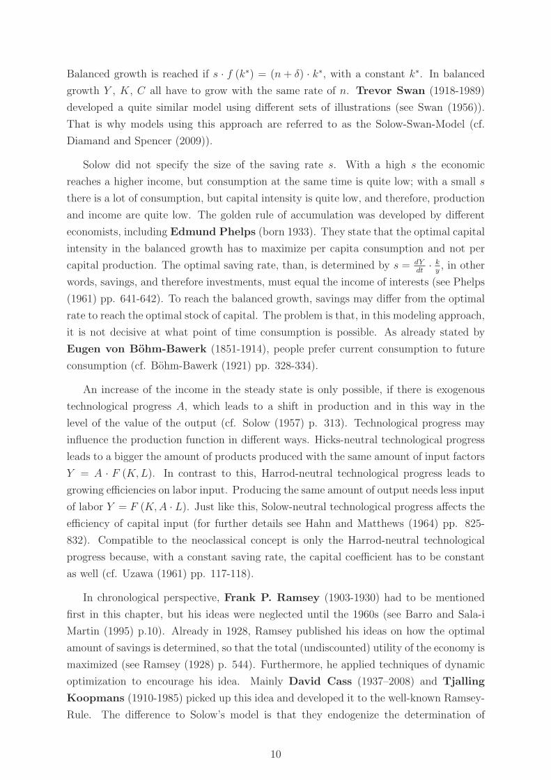
Balanced growth is reached if s · f (k∗) = (n+ δ) · k∗, with a constant k∗. In balanced

growth Y , K, C all have to grow with the same rate of n. Trevor Swan (1918-1989)

developed a quite similar model using different sets of illustrations (see Swan (1956)).

That is why models using this approach are referred to as the Solow-Swan-Model (cf.

Diamand and Spencer (2009)).

Solow did not specify the size of the saving rate s. With a high s the economic

reaches a higher income, but consumption at the same time is quite low; with a small s

there is a lot of consumption, but capital intensity is quite low, and therefore, production

and income are quite low. The golden rule of accumulation was developed by different

economists, including Edmund Phelps (born 1933). They state that the optimal capital

intensity in the balanced growth has to maximize per capita consumption and not per

capital production. The optimal saving rate, than, is determined by s = dYdt

·ky, in other

words, savings, and therefore investments, must equal the income of interests (see Phelps

(1961) pp. 641-642). To reach the balanced growth, savings may differ from the optimal

rate to reach the optimal stock of capital. The problem is that, in this modeling approach,

it is not decisive at what point of time consumption is possible. As already stated by

Eugen von Bohm-Bawerk (1851-1914), people prefer current consumption to future

consumption (cf. Bohm-Bawerk (1921) pp. 328-334).

An increase of the income in the steady state is only possible, if there is exogenous

technological progress A, which leads to a shift in production and in this way in the

level of the value of the output (cf. Solow (1957) p. 313). Technological progress may

influence the production function in different ways. Hicks-neutral technological progress

leads to a bigger the amount of products produced with the same amount of input factors

Y = A · F (K,L). In contrast to this, Harrod-neutral technological progress leads to

growing efficiencies on labor input. Producing the same amount of output needs less input

of labor Y = F (K,A · L). Just like this, Solow-neutral technological progress affects the

efficiency of capital input (for further details see Hahn and Matthews (1964) pp. 825-

832). Compatible to the neoclassical concept is only the Harrod-neutral technological

progress because, with a constant saving rate, the capital coefficient has to be constant

as well (cf. Uzawa (1961) pp. 117-118).

In chronological perspective, Frank P. Ramsey (1903-1930) had to be mentioned

first in this chapter, but his ideas were neglected until the 1960s (see Barro and Sala-i

Martin (1995) p.10). Already in 1928, Ramsey published his ideas on how the optimal

amount of savings is determined, so that the total (undiscounted) utility of the economy is

maximized (see Ramsey (1928) p. 544). Furthermore, he applied techniques of dynamic

optimization to encourage his idea. Mainly David Cass (1937–2008) and Tjalling

Koopmans (1910-1985) picked up this idea and developed it to the well-known Ramsey-

Rule. The difference to Solow’s model is that they endogenize the determination of

10

the optimal amount of savings and explicitly model the consumer side (see Cass (1965)

and Koopmans (1963)). Koopmans uses a discounted utility function with an infinite

time horizon to determine the optimal path of consumption and investment under the

individuals’ budget constraint (see Koopmans (1963) pp. 22-23). Specific information on

the behavior of the optimal saving rate can only be given with additional assumptions

concerning the utility and the production function (see Cass (1965) p. 238), but generally

it can be said that the saving rate is now determined by the interest rate and is not given

exogenously. Beginning with a given stock of capital, there is only one existing optimal

allocation path to reach the steady state, where stock of capital grows with the same

intensity as the labor input. Keeping in mind that the utility is now discounted, the

optimal stock of capital per capita in the steady state is smaller than in the Solow model.

Using Samuelson’s idea, Peter Diamond (born 1940) introduced the overlapping

generations in neoclassical growth theory (Samuelson (1958) and Diamond (1965)). He

extended the set-up used by Cass and Koopmans by introducing individuals with finite

time horizon. Individuals are continuously dying, and new agents are born. Individuals

have different saving rates in different stages of life. It is assumed that individuals save

an amount of their income in the first period of life, which generates the capital stock in

the next period. During the second period of life, they receive income from the capital

stock, which is completely consumed. The decision of the saving rates, which depends on

the time preferences, has to be made, taking into consideration the growing population

and the growing demand.

John von Neumann (1903-1957) develops a linear economic model of growth. His

main contribution was the mathematical approach to prove the existence and uniqueness

of equilibrium of an expanding economy. In contrast to the other models, Neumann (1945)

uses a production function, where the final goods are produced with the same products

as input factors, and a decision has to be made which of the different available production

technologies is used. The important parameter is to define with which intensity the chosen

technologies have to be used to maximize total production (cf. Neumann (1945) p. 2).

The fact of producing and developing these technologies is not considered. The difficulty

is to find the set where the demand for all goods (for production and consumption) and

the supply of these goods are balanced. The equilibrium is reached, when the economy

expands without any change in the production structure (cf. Hahn and Matthews (1964)

p. 855).

3.4 Evolutionary Theory

In the 1980s a new approach of explaining the technological change influencing economic

growth was developed. The evolutionary theory designs the economic process similar

11

to the biological evolution. There is one market, and the ongoing competition between

products, companies and even economic systems leads to the situation that only those

will survive which fit the needs best and adjust themselves best to changing conditions.

Based on the ideas published by Friedrich von Hayek (competition as discovery of

new possibilities (see v. Hayek (1969)) and by Schumpeter (1883-1950) (theory creative

destruction (see chapter 2.2 of this paper)), it is possible that changes and innovations will

cause the destruction of ideas and products. The evolutionary theory was established as

a separate research field after the critique of Nelson and Winter on the basic question

of how firms and industries change overtime, giving an answer with evolutionary theory

background (see Nelson and Winter (1982)).

4 Endogenous Growth Theory

The neoclassical approaches were quite unsatisfactory because the main vari-

able explaining economic growth, the rate of technological progress, was ex-

ogenously given. The results did not fit to the empirical data and the eco-

nomical insight that technological progress depends on economic decisions.

Furthermore, if the rate of technological progress is exogenously given, it must

be the same for all countries, and differences between countries would van-

ish. A new field of research, a new neoclassical approach or the endogenous

growth theory, developed, trying to explain technological progress endoge-

nously. The main problem was how to deal with the possibility of increasing

returns, keeping in mind that under these conditions not all factors can be

paid the marginal factor product (see Aghion and Howitt (1998) p. 23). The

different ideas to overcome these problems are already listed an assorted by

Romer (1994) and described in detail by Jones and Manuelli (1997). In the

next sections the main aspects are explained, concentrating on the authors’

different assumptions.

4.1 Leading Towards Endogenous Growth

Young can be seen as one of the forerunners of endogenous growth (see chapter 2.2 of this

paper). He already insists on the assertion that growth is endogenous and cumulative

and the main source of growth is growth itself (cf. Sandilands (2000) p. 309). Already

Nordhaus (born 1941) stated that it is not satisfying or rather not correct to say that

economic growth is induced by technological progress because it cannot be determined

what leads to economic growth. It is more precise to say that the growth of the input

factors cannot fully explain the growth of the output and that there have to be other

12

driving forces (see Nordhaus (1969) p. 18). As a consequence, he claims for theories that

explain the generation and transmission of new knowledge and for that reason are able to

define the forces leading to productivity changes. In a first attempt to achieve this aim,

Nordhaus defines technological change as depending on the number of inventions made,

which in turn depend on the amount of output devoted to invention. A new result is

that a rising technological change leads to reduction of the capital stock. The problem of

this model is that there has to be population growth in a first step to start the process

of a growing number of inventions. A growing amount of output in real terms must

be devoted to invention production because diminishing returns are assumed; otherwise

technology will stagnate (ibidem p.23). Karl Shell (born 1938) introduced an invention

sector in almost the same manner, thereby concentrating on the organizational matters

as monopoles and the properties of pure public goods (Shell (1973)).

4.2 Endogenous Growth Using Capital Accumulation

One of the simplest ideas to overcome the exogenous explanation of economic growth

is relaxing some assumptions of the Solow model. Now the marginal productivity of

capital convergences to a positive value A > 0, and therefore, production becomes a linear

equation depending on capital, in the Cobb-Douglas case this reads Y = AK. This kind of

model is known as the AK-approach. Sergio Rebelo (born 1959) chooses this approach

in his basic growth model, using a very wide capital definition including both physical

and human capital (cf. Rebelo (1991) pp. 502-503). In this case, growth is professed

by always positive marginal returns to capital, which seems to be unrealistic. As in the

linear Neumann Model, technological progress is completely left out of consideration.

Larry Jones and Rodolfo Manuelli add to the production function a further term to

incorporate further input factors, Y = AK + f (K,L) (cf. Jones and Manuelli (1990)

p. 1014). But these factors cannot be essential to production because otherwise the

assumption of steady positive values of the marginal productivity cannot be maintained.

It might decrease in the beginning, but with rising capital intensity it convergences to A

again.

4.3 Technological Progress Using Spillover Effects

The main idea is that there must be a difference between productions seen from the

point of view of an individual firm compared to the perspecitve of the whole economy.

From the individual’s view, the state of the technology is exogenously given, and even the

progress might seem to be exogenous because discoveries may be accidental and not always

based on individual decisions. But from an external view, the technological progress is

endogenous because it is influenced by the decisions and efforts made by individuals (cf.

13

Romer (1994) pp. 13-14). There are externalities from the individual behavior to the

total stock of knowledge and reverse.

One of the first endogenous growth models is “Increasing Returns and Long-Run

Growth” (1986) introduced by Paul M. Romer (born 1955). He models technological

progress as depending on the total amount of investments to knowledge A (R), which is

determined by individual decisions of each competitive firm j. Investments can be either

done in the capital of the firms or in individual research, increasing private knowledge Rj.

Investing one unit into research enlarges the stock of knowledge not only by one unit, but

rather more, depending on the current stock of private knowledge (cf. Romer (1986) p.

1019). The output of the individual firms then reads Yj = A (R) ·F (Rj, Kj, Lj), depend-

ing on the total stock of knowledge and the individual inputs, including investments to

knowledge (cf. Romer (1994) p. 15). To prevent the production function from increasing

returns, the private stock of knowledge is assumed to be rival, and therefore, has to be

enlarged to achieve more output. The spillovers from the private stocks of knowledge

Rj to the total stock of knowledge R describe the endogenization of the technological

progress. For the individual firm, the stock of total knowledge is exogenously given, but

it is determined by individual decisions.

Another early and quite similar model was developed by Kenneth J. Arrow (born

1921). He stated that the technological progress is influenced by the investments to capital

in each period and called it the experience generated by using the goods acquired by the

capital stock (cf. Arrow (1962) p. 157 and p. 172). The production function changes to

Yj = A (K) · F (Kj, Lj). In this case the endogenization of the technological progress is

a by-product of the production process and the choice of the investment rate, and not

directly influenced by an individual decision. Robert Lucas (born 1937) developed a

similar model, distinguishing between physical capital K and human capital H. In this

case, there are two individual investment decisions. Investments in human capital are

generated by devoting time to learning and reaching a higher skill level (cf. Lucas (1988)

p. 18). The technological progress is determined by the individual investments into

human capital, therefore Yj = A (H) · F (Kj, Hj) (see additionally for the whole section

and especially the equations Romer (1994) p. 15).

The idea of the following models was to explain the differences of income per capita

in different countries. To explain the different growth rates the assumption that the

same technological opportunities are available at all times for everyone must be dropped

(see Romer (1994) p. 4). He also gives one of the first solutions to model this. He

predicates that the technological progress depends positively on the amount of capital

in the respective country and negatively on the amount of labor. The negative effect

results from the fact that, with a higher amount of labor it becomes unattractive to

drive technological progress in labor saving innovations A (K,L) = KγL−γ. Using a

14

Cobb-Douglas production function, as Y = A (K,L) ·Kα · L1−α, the total output reads

Y = K1−βLβ with β = α − γ. Now the size of β is determining if and to what extend

different economies converge (Barro and Sala-i Martin (1992)). Additionally, they explain

the differences in the possible steady state by further variables included in A, like e.g. the

school enrollment rates and political revolutions (ibidem p. 242, Table 3). Mankiw et al.

(1992) assume that the technological level is the same in all economies, but that there is

a further input factor of human capital, which represents the additional variables. Those

were also used by Robert J. Barro (born 1944) and Xaviar Sala i Martin (born

1962) (Mankiw et al. (1992) p. 11).

4.4 Innovation as Engine of Growth

A further approach in endogenous growth theory, which is mainly used today, is to model

explicitly technological innovation and investments to research and development. There

are two different manners how this influences the production, either by increasing the

variety of products or by improving the quality of products. A characteristic of these

models is that they take into account that the firms will only invest in research and

development if there is a chance to use the innovation exclusively and that they have at

least a temporary monopoly.

One of the best known models is introduced by Paul Romer in 1990. Using the

production variety theory of Avinash Dixit (born 1944) and Joseph E. Stiglitz (born

1963), he creates a model where innovations lead to new products or new technologies;

the variety of products is increasing (horizontal innovation) (Dixit and Stiglitz (1977),

Romer (1990)). To overcome the critique that obsolescence is not taken into account,

vertical innovations, where the qualities of products and processes are improved, and

therefore, old products substituted, are considered (Grossman and Helpman (1991) and

Aghion and Howitt (1992)). Gene Grossman (born 1955) and Elhanan Helpman

(born 1946) introduce quality ladders for each product, which are followed during the

innovation process. Philippe Aghion (born 1956) and Peter Howitt (born 1946) take

up again Schumpeter’s idea of creative destruction (see chapter 2.2 of this paper).

The main setup of these models is quite similar. The economy consists of three

sectors, one producing innovations, the second producing intermediates and the third

one manufacturing the final output. Using human capital, a distinction between working

people’s individual knowledge H, which is rival in use, and the technological level A,

which is non-rival, has to be made (see Romer (1990) p. S79). In the research sector a

share of human capital HA and the current stock of knowledge are used to produce new

ideas and templates (in the case of Romer) or new prototypes with better qualities (in

the other case), A = F (A,HA). Then a different firm in the sector of the intermediates

15

bids to get the right to combine the output of the research sector with further investment

goods (foregone output) to produce goods required by the final production xi. In this

case, the intermediates producer has at least a temporary monopoly and the innovations

can be paid (see Aghion and Howitt (1992) p. 328). The remainder of human capital

HY , labor L and physical capital K, which consist of the different intermediates xi, are

the input used for final production, therefore total output is Y = F (HY , L,∑

xi∞

i=0).

The growth engine of these models is that there are sectors which use their own output

as input. In the research sector mainly labor or a share of human capital is used as direct

input, combined with the total stock of the technical knowledge of the society influencing

the productivity of the used labor. The output of the research sector is the new technical

knowledge which is added to the current stock. Additionally, the assumption of non-

decreasing returns to the direct or indirect inputs is needed to generate positive growth

per capita (see Groth (2007) p. 130). Due to the fact that Schumpeter was one of the first

to have the idea that a temporary monopoly is essential to motivate innovations and that

new inventions may make old technologies inefficient, growth models incorporating this

are called models of neo-Schumpeterian growth (see Aghion and Howitt (1998) chapter

2).

4.5 Further Endogenous Growth Models

Today, the theory of endogenous growth is the main theory used to analyze economic

growth. It is used as a basis for further research in many fields and focusing on many

different concrete aspects (for an overview on the different aspects in endogenous growth

theory see Jones and Manuelli (1997)). Researchers try to incorporate more input fac-

tors into the production function to reach more realistic results and to reveal different

coherences between growth and the assumptions made to model these input factors. For

example, the human capital sector is more specified by incorporating inelastic supply,

leisure time, education or unemployment. Another field of economic research incorpo-

rates the government as a further producing sector, producing public goods, or as political

institution, making different requirements or giving assistance. Different market struc-

tures and sizes and even open economies, including international trade, are considered

as well. In recent years, quite a lot of research deals with the effect of natural resources,

keeping sustainability and environmental facts in mind (see next section).

Different sectors are added to reflect the economy of a single country or region with

the intention to receive more realistic models. The different sectors react differently on

economic decisions, and different production coefficients are assumed (for an introduction

to multisector growth models see Roe et al. (2010)). The rising complexity of these models

requires computational methods. They are introduced in economic growth theory in

16

order to solve these problems and make numerical simulations possible. Additionally, not

only deterministic models are solved; stochastic parameters are introduced. Doing so,

the normal uncertainty of economic development and further uncontrollable influencing

factors are incorporated. Now the expected utility becomes the object of maximization

(see Heer and Maußner (2009) pp. 27-33 for an example of a stochastic Ramsey model).

A further field of research deals with supplementary empirical studies, which are made

to confirm or refuse these expansions to the models and to verify the accompanying

assumptions. Testing the theoretical results in comparison to real data sets leads to

better assumptions concerning the different variables. Today more and more data are

gathered and edited for research purpose. With the help of today’s computer capacities,

it is possible to test huge sets of data and compare the results of different sets of variables

to each other. Additionally, the value of the different variables may be estimated. It is

possible to isolate unusual and non-recurrent events, and therefore, future predictions

become more stalwart, as far as they are determined by the past.

5 Natural Resources and Growth

In recent decades the inter-temporal allocation of exhaustible resources has

been a frequently discussed topic, especially in the context of sustainable

economic growth. In this context, sustainability is defined as leading to inter-

generational justice, meaning that future generations may not be put into a

worse position. But that does not mean that all resources have to be kept un-

touched and cannot be used; rather all consequences of the use (like finiteness

and environmental impact) and all substitution possibilities should be taken

into account (for a further definition see Aghion and Howitt (1998) p. 155-

157). During the last years the use of renewable resources is as well discussed

critically because of the competition of land used for cultivation of renewable

energy resources and the land used for food production.

5.1 Beginning of Resource Theory

The economists who developed the first economical theories were confronted with a com-

pletely different set of production. Agricultural products were the main goods produced

by using natural resources. The concern that resources would not last forever and might

be fully exploited was of no vital significance. In the classical perspective, land was the

main scarce factor, which would lead to diminishing returns and economic stagnation (see

Ricardo chapter 2.1 and cf. Groth (2007) p. 127). This period is followed by the first

systematic approaches to resource theory keeping in mind both, nonrenewable resources

17

and renewable resources. In 1849 Martin Faustmann (1844-1876) formulates one of

the first optimal rules for reforestation (timber as renewable resource), while trying to

determine the maximum value of forest floor (Faustmann (1849)); but it was not until

1921 that Bertil Ohlin (1899-1979) formulated the mathematical conditions describing

this rule (Ohlin (1995)). An early approach to the economics of nonrenewable resources,

which is seldom cited, is evolved by Gray in 1913. He points out the importance of con-

servation of resources, especially of those which are exhausted by use and non-restorable

after exhaustion, and the conflict between present and future use (cf. Gray (1913) pp.

499-501). His work is followed by Harold Hotelling’s (1895-1973) famous work on the

economics of exhaustible resources, where he revealed the still used Hotelling Rule. He

provided a rule to maximize the present value of all future profits for the owner of an

exhaustible supply (cf. Hotelling (1931) p. 140). The amount extracted has to be chosen

in a way that the price of the resource increases at the rate of interest. This leads to the

result that the stock of the resource is not extracted completely as soon as possible.

In the beginning, neoclassical economics dealing with economic growth almost com-

pletely neglected natural resources. Until the 1970s, the pessimistic Malthusian view

that the limited stock of non-renewable resources would restrict the economic growth

was dominant. Especially the predictions of the Club of Rome emphasized these nega-

tive predictions (see Meadows et al. (1972)). They warn that the optimistic assumptions

of economic growth will not last for long, due to the rising world population and the

associated rising food demand. Additionally, they focus on the increasing environmen-

tal damage and the limited stocks of important resources. By introducing resources as

essential input to production in the neoclassical growth framework, this view could be

overcome to some extent because economic growth now was seen as possible as long as

there was a sufficient rise in the technical progress. Until then, land was seen as the re-

stricting factor for growth (see Ricardo in chapter 2.2 of this paper). Land is introduced

as a non-reproducible factor, the same amount of which is available in each period (cf.

Rebelo (1991) p. 502). Using land as an input factor in the Solow model (see chapter

3.3 of this paper), leads to the result that the growth rates of output and technological

progress now differ from each other. The growth rate of total output is now depending

on the exogenous technological growth less the production coefficient of land β times

the population growth n (gY = g (P,−β · n), cf. Jones (2002) pp. 172-173). In this

model land exhibits diminishing returns because it is used as a fixed factor; technological

progress, if high enough, may compensate this.

But in the neoclassical view definitve answers could not be given as long as techno-

logical progress was seen as exogenous. The increase of research, including the dealing

with natural resource, was driven by the oil crisis in the mid-1970s. In a symposium

issue of Review of Economic Studies in 1974, the basic articles considering non-renewable

resources R in economic growth models were published (for a summery see Krautkraemer

18

(1998) pp. 2091-2095). They are all starting from the same main assumptions and then

concentrate on different aspects (cf. Groth (2007) pp. 135-142). A neoclassical produc-

tion function with constant returns to scale and exogenous technological progress is used.

There is a fixed amount of cumulative resource extraction for all times. If population

growth is considered, the largest consumption per head which lasts to eternity must be

found, keeping in mind the finiteness of the non-renewable resource (cf. Solow (1974)

p. 35). There are different possibilities to do so; the non-renewable resource may be

substituted by capital or other resources, there might be resources-augmenting technical

progress, or increasing returns to scale (cf. Neumeyer (2000) p. 307).

There is only one state where the capital-output ratio K/Y and the ratio of used

resource to resource stock R/S are constant. It can only be reached if the rate of technical

progress is greater than the share of the resource multiplied by the rate of population

growth, which means resource augmenting technological progress (Stiglitz (1974a,b)). In

case the economy departs from this path, there exists a finite time horizon after which

consumption stops growing and the resource is fully exhausted. Furthermore, it is not

certain whether resource augmenting technical progress is permanently possible and is

sufficient to replace the declining stock of the resource (cf. Neumeyer (2000) p. 325).

Dasgupta and Heal (1974) use a quite different approach to solve the same problem.

They use a CES production function; in the case of the substitution parameter σ ≤ 1 the

non-renewable resources are essential to production. The production and consequently

the consumption level first rises, but tends to zero during time. If σ > 1, there is no

problem because the resource is inessential for production. To overcome the result of

declining output, technical change is introduced at a specific date T , when a perfect

substitute for the non-renewable resource, in form of a flow of services at a constant rate,

is discovered (cf. Dasgupta and Heal (1974) p. 7). At point T the economy switches,

and production and consumption rise again.

5.2 Including Resources in Economic Growth Models Today

Again the approach, starting from the assumption that technological progress is only

exogenously given, is not satisfying. That is why models postulating endogenous tech-

nological progress and including natural resources were developed. The different basic

ideas are summarized by Aghion and Howitt (1998), chapter 5.They incorporate a non-

renewable resource to the AK-model (see chapter 4.2 of this paper) and to the Schum-

peterian approach (see chapter 3.4 of this paper); and at the same time they take into

account the state of the environment. In all approaches innovations and technological

progress are used as a necessary input in order to be able to reach an optimal sustainable

growth path. This is seen to be possible; but the question is, how it can be reached and

19

which institutions have to be introduced (cf. Aghion and Howitt (1998) pp. 164-165).

Grimaud and Rouge (2003) develop a model using the approach of Aghion and Howitt

(1992) incorporating a non-renewable resource and using labor either for final production

or for research. Under certain conditions an equilibrium growth path can be revealed,

but the outcome may either be positive or negative, depending on the discount rate of

the economy in relation to the parameters of the research function (cf. Grimaud and

Rouge (2003) p. 452). Further approaches were made for example by Scholz and Ziemes

(1999) and Schou (2000). The basic results of these models are all quite similar to those,

when no non-renewable resource is used, because the resources do not enter the growth

engine, the research sector (cf. Groth (2007) p. 150). An idea to solve these critiques

is presented by Groth (2005). He introduces the non-renewable resource not only into

the production function of the final output but also as input to the research activity (see

ibidem pp. 3-4). In this case there must be population growth and a high elasticity of

output to knowledge to compensate for the declining resource input.

It seems that when using renewable resources in an economic growth model instead

of non-renewable ones there are no big differences to a model where resources are not

considered. As long as the regeneration capacity of the resource ηA is higher than the

demand of the resource for production, and no further input or output is observed, this

is true (cf. Aznar-Marquez and Ruiz-Tamarit (2005) p. 180). But in the context of re-

newable resources further extensions have to be kept in mind. Depending on the chosen

production function, a higher input of a resource leads to a higher output and therefore

to higher growth. It would be reasonable to use as much renewable resource as possible,

but in the context of sustainable growth, the regeneration capacity is a limiting factor.

Additionally, a further influencing factor is the allocation of labor between harvesting the

resource and its use in the final output sector (cf. Elıasson and Turnovsky (2004) pp.

5-6). Another approach is to model the sensitiveness of the resource regeneration to envi-

ronmental pollution arising from final good production (cf. Tahvonen and Kuuluvainen

(1991) pp. 651-652). But pollution may also be generated by the production and use of

the resources (both by renewable or by non-renewable ones). Furthermore, it is discussed

if a growing use of renewable resources and therefore, an expansion of production, is after

all desirable because the land used for resource production is in competition to the land

used for food production (cf. Kuhn et al. (2013) p. 471).

6 Outlook

We can see that for a long time the basic theories for economic growth were subject to

enormous changes, influenced by the different stages of the societies. As the existing

theories were not satisfying in the new context or did not fit to undergone experiences,

20

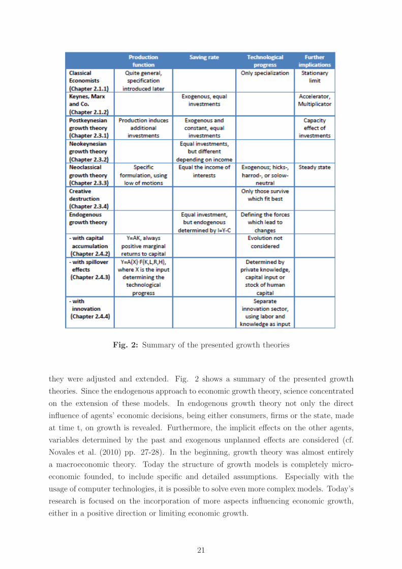
Fig. 2: Summary of the presented growth theories

they were adjusted and extended. Fig. 2 shows a summary of the presented growth

theories. Since the endogenous approach to economic growth theory, science concentrated

on the extension of these models. In endogenous growth theory not only the direct

influence of agents’ economic decisions, being either consumers, firms or the state, made

at time t, on growth is revealed. Furthermore, the implicit effects on the other agents,

variables determined by the past and exogenous unplanned effects are considered (cf.

Novales et al. (2010) pp. 27-28). In the beginning, growth theory was almost entirely

a macroeconomic theory. Today the structure of growth models is completely micro-

economic founded, to include specific and detailed assumptions. Especially with the

usage of computer technologies, it is possible to solve even more complex models. Today’s

research is focused on the incorporation of more aspects influencing economic growth,

either in a positive direction or limiting economic growth.

21

Since the beginning of the 21st century, non-renewable but also renewable resources

become more and more an important input factor to models of economic growth. Against

the background of scarce resource, sustainable development and environmental issues, it

is essential to integrate the economic resource theory into growth theory to reveal the

influences on economic growth.

References

Aftalion, A. (1927). The Theory of Economic Cycles Based on the Capitalistic Technique

of Production. The Review of Economics and Statistics, 9 (4), 165–170.

Aghion, P. and Howitt, P. (1992). A Model of Growth Through Creative Destruction.

Econometrica, 60 (2), 323–351.

Aghion, P. and Howitt, P. (1998). Endogenous Growth Theory. Cambridge and Mas-

sachusetts: The MIT Press.

Arrow, K. J. (1962). The Economic Implications of Learning by Doing. The Review of

Economic Studies, 29 (3), 155–173.

Aznar-Marquez, J. and Ruiz-Tamarit, J. R. (2005). Renewable Natural Resources and

Endogenous Growth. Macroeconomic Dynamics, 9 (2), 170–197.

Barro, R. J. and Sala-i Martin, X. (1992). Convergence. Journal of Political Economy,

100 (2), 223–251.

Barro, R. J. and Sala-i Martin, X. (1995). Economic Growth. New York: McGraw-Hill

Inc.

Bohm-Bawerk, E. v. (1921). Kapital und Kapitalzins: Abt. Positive Theorie des Kapitales

(4th ed.). Kapital und Kapitalzins. G. Fischer.

Bretschger, L. (2004). Wachstumstheorie (3rd ed.). Munchen: Oldenbourg Wis-

senschaftsverlag.

Bundesministerium der Justiz (1967). Gesetz zur Forderung der Stabilitat und des

Wachstums der Wirtschaft. http://bundesrecht.juris.de/bundesrecht/ stabg/gesamt.pdf,

26.05.2014.

Cass, D. (1965). Optimum Growth in an Aggregative Model of Capital Accumulation.

The Review of Economic Studies, 32 (3), 233–240.

CIA - Central Intelligence Agency (2010). The World Factbook: Country Compar-

ison: GDP Real Growth Rate. https://www.cia.gov/library/publications/the-world-

factbook/rankorder/rankorderguide.html, 26.05.2014.

22

Clark, J. M. (1917). Business Acceleration and the Law of Demand: A Technical Factor

in Economic Cycles. Journal of Political Economy, 25 (3), 217–235.

Currie, L. (1981). Allyn Young and the Development of Growth Theory. Journal of

Economic Studies, 8 (1), 52–60.

Dasgupta, P. and Heal, G. (1974). The Optimal Depletion of Exhaustible Resources. The

Review of Economic Studies, 41 (5), 3–28.

Diamand, R. W. and Spencer, B. J. (2009). Trevor Swan and the Neoclassical Growth

Model. In History of Political Economy, volume 41 (pp. 107–126). Duke Univerity

Press.

Diamond, P. A. (1965). National Debt in a Neoclassical Growth Model. The American

Economic Review, 55 (5), 1126–1150.

Dixit, A. K. and Stiglitz, J. E. (1977). Monopolistic Competition and Optimum Product

Diversity. The American Economic Review, 67 (3), 297–308.

Domar, E. (1946). Captial Expansion, Rate of Growth, and Employment. Econometrica,

14 (2), 137–147.

Elıasson, L. and Turnovsky, S. (2004). Renewable Resources in an Endogenously Growing

Economy: Balanced Growth and Transitional Dynamics. Journal of Environmental

Economics and Management, 3 (48), 1018–1049.

Eltis, W. (1975). Francois Quesnay: A Reinterpretation: 2. The Theory of Economic

Growth. Oxford Economic Papers, 27 (3), 327–351.

Eltis, W. (1989). David Ricardo. In J. Starbatty (Ed.), Klassiker des okonomischen

Denkens, volume 1 (pp. 188–207). Munchen: Beck.

Faustmann, M. (1849). Berechnung des Werthes, welchen Waldboden, sowie noch nicht

haubare Holzbestande fur die Waldwirtschaft besitzen. Allgemeine Forst- und Jagd-

Zeitung, 15, 441–451.

Gray, L. C. (1913). The Economic Possibilities of Conservation. The Quarterly Journal

of Economics, 27 (3), 497–519.

Grimaud, A. and Rouge, L. (2003). Non-renewable Resources and Growth with Vertical

Innovations: Optimum, Equilibrium and Economic Policies. Journal of Environmental

Economics and Management, 45 (2), 433–453.

Grossman, G. M. and Helpman, E. (1991). Quality Ladders in the Theory of Growth.

The Review of Economic Studies, 58 (1), 43–61.

23

Groth, C. (2005). Growth and Non-renewable Resources Revisited. Working Paper

University of Copenhagen, 1–31.

Groth, C. (2007). A New-Growth Perspective on Non-Renewable Resources. In

L. Bretschger and S. Smulders (Eds.), The Economics of Non-Market Goods and Re-

sources, volume 10 (pp. 127–163). Springer.

Hahn, F. H. and Matthews, R. (1964). The Theory of Economic Growth: A Survey. The

Economic Journal, 74 (296), 779–902.

Hamberg, D. and Schultze, C. L. (1961). Autonomous vs. Induced Investment: The

Interrelatedness of Parameters in Growth Models. The Economic Journal, 71 (281),

53–65.

Harrod, R. (1939). An Essay in Dynamic Theory. Economic Journal, 49 (193), 14–33.

Heer, B. and Maußner, A. (2009). Dynamic General Equilibrium Modeling: Computa-

tional Methods and Applications (2nd ed., corr. 2nd printing ed.). Berlin: Springer.

Heertje, A. and Wenzel, H.-D. (2008). Grundlagen der Volkswirtschaftslehre (7th ed.).

Berlin and Heidelberg: Springer.

Holub, H.-W. (2010). Eine Einfuhrung in die Geschichte des okonomischen Denkens:

Band III: Physokraten und Klassiker (2nd ed.). Munster and Berlin and Wien: LIT

Verlag.

Hotelling, H. (1931). The Economics of Exhaustible Resources. Journal of Political

Economy, 39 (2), 137–175.

Jones, C. I. (2002). Introduction to Economic Growth (2nd ed.). New York: W. W.

Norton & Company.

Jones, L. E. and Manuelli, R. E. (1990). A Convex Model of Equilibrium Growth: Theory

and Policy Implications. Journal of Political Economy, 98 (5), 1008–1038.

Jones, L. E. and Manuelli, R. E. (1997). The Sources of Growth. Journal of Economic

Dynamics and Control, 21 (1), 75–114.

Kaldor, N. (1957). A Model of Economic Growth. The Economic Journal, 67 (268),

591–624.

Keynes, J. M. (1936). The General Theory of Employment Interest and Money. London:

Macmillan Press.

Koopmans, T. C. (1963). On the Concept of Optiomal Economic Growth. Cowles Foun-

dation Discussion Paper, (163), 1–37.

24

Krautkraemer, J. A. (1998). Nonrenewalbe Resource Scarcity. Journal of Economic

Literature, 36 (4), 2065–2107.

Kuhn, T., Pickhardt, M., and Voosholz, F. (2013). Energy Policy, Food, and Climate

Change–A Numerical Simulation Approach. Procedia Economics and Finance, 5, 468–

477.

List, F. (1841). Das Nationale System der Politischen Okonomie. Stuttgart: Cotta

Verlag.

Lucas, R. E. J. (1988). On the Mechanics of Economic Development. Journal of Monetary

Economics, 22 (1), 3–42.

Malthus, R. (1798). An Essay on the Principle of Population. London: J. Johnson, in

St. Paul’s Church-Yard.

Mankiw, G. N., Romer, D., and Weil, D. N. (1992). A Contribution to the Empirics of

Economic Growth. The Quarterly Journal of Economics, 107 (2), 407–437.

Marchi, N. d. (1989). John Stuart Mill. In J. Starbatty (Ed.), Klassiker des okonomischen

Denkens, volume 1 (pp. 266–290). Munchen: Beck.

Marshall, A. (1980). Principles of Economics: The Agents of Production (8th ed.).,

volume 4 of Principles of Economics. London: Macmillan Press.

Marx, K. (1962). Das Kapital - Kritik der politischen Okonomie: Band II: Der Zirku-

lationsprozess des Kapitals. In F. Engels (Ed.), Marx-Engels-Werke, volume 24 (pp.

7–518). Berlin/DDR: Dietz Verlag.

Meadows, D. H., Meadows, D. L., Randers, J., and Behrens, W. W. I. (1972). The Limits

to Growth. A Report for the Club of Rome’s Project on the Predicament of Mankind.

New York: Universe Books.

Meyer, E., Muller-Siebers, K.-W., and Strobele, W. (1998). Wachstumstheorie (2nd ed.).

Munchen and Wien: Oldenbourg Wissenschaftsverlag.

Mill, J. S. (1848). Principles of Political Economy (7th ed.). London: Longmans, Green

and Co.

Murad, A. (1962). What Keynes Means. New York: Bookman Associates.

Nelson, R. R. and Winter, S. G. (1982). An Evolutionary Theory of Economic Change.

Cambridge: Harvard University Press.

Neumann, J. v. (1945). A Model of General Economic Equilibrium. The Review of

Economic Studies, 13 (1), 1–9.

25

Neumeyer, E. (2000). Scare or Abundant? The Economics of Natural Resource Avail-

ability. Journal of Economic Surveys, 14 (3), 307–335.

Nordhaus, W. D. (1969). An Economic Theory of Technological Change. The American

Economic Review, 59 (2), 18–28.

Novales, A., Fernandez Casillas, E., and Ruız, J. (2010). Economic Growth: Theory and

Numerical Solution Methods (1st ed.). Berlin: Springer.

Ohlin, B. (1995). Concerning the Question of the Rotation Period in Forestry (translated

from the original, 1921). Journal of Forest Economics, 1, 89–114.

Phelps, E. (1961). The Golden Rule of Accumulation: A Fable for Growthmen. The

American Economic Review, 51 (4), 638–643.

Quesney, F. (1965). Tableau Economique (3rd ed. 1759). Berlin: Akademie Verl.

Ramsey, F. P. (1928). A Mathematical Theory of Saving. The Economic Journal, 38 (152),

543–559.

Rebelo, S. (1991). Long-Run Policy Analysis and Long-Run Growth. Journal of Political

Economy, 99 (3), 500–521.

Ricardo, D. (1821). On the Principles of Political Economy and Taxation (3rd ed.).

London: John Murray.

Roe, T. L., Saracoglu, D. S., and Smith, R. B. W. (2010). Multisector Growth Models:

Theory and Application. New York and NY: Springer-Verlag New York.

Rogers, M. (2003). A Survey of Economic Growth. The Economic Record, 79 (244),

112–135.

Romer, P. M. (1986). Increasing Returns and Long-Run Growth. Journal of Political

Economy, 94 (4), 1002–1037.

Romer, P. M. (1990). Endogenous Technological Change. Journal of Political Economy,

98 (5), S71–S102.

Romer, P. M. (1994). The Origins of Endogenous Growth. Journal of Economic Per-

spectives, 8 (1), 3–22.

Rostow, W. W. (1959). The Stages of Economic Growth. The Economic History Review,

12 (1), 1–16.

Samuelson, P. A. (1939). Interactions between the Multiplier Analysis and the Principle

of Acceleration. The Review of Economics and Statistics, 21 (2), 75–78.

26

Samuelson, P. A. (1958). An Exact Consumption-Loan Model of Interest with or without

the Social Contrivance of Money. Journal of Political Economy, 66 (6), 467–482.

Sandilands, R. J. (2000). Perspectives on Allyn Young in Theories of Endogenous Growth.

Journal of History of Economic Thought, 22 (3), 309–328.

Scholz, C. M. and Ziemes, G. (1999). Exhaustible Resources, Monopolistic Competition,

and Endogenous Growth. Environmental and Resource Economics, 13 (2), 169–185.

Schou, P. (2000). Polluting Non-Renewable Resources and Growth. Environmental and

Resource Economics, 16 (2), 211–227.

Schumpeter, J. (1934). Theorie der wirtschaftlichen Entwicklung (4th ed.). Berlin:

Duncker & Humbot.

Shell, K. (1973). Inventive Activity, Industrial Organization and Economic Growth. In

J. A. Mirrlees and N. Stern (Eds.), Models of Economic Growth (pp. 77–100). London:

Macmillan Press.

Smith, A. (1776). An Inquiry into the Nature and Causes of the Wealth of Nations. Basel:

J. J. Tourneisen.

Solow, R. M. (1956). A Contribution to the Theory of Economic Growth. The Quarterly

Journal of Economics, 70 (1), 65–94.

Solow, R. M. (1957). Technical Change and the Aggregate Production Function. The

Review of Economics and Statistics, 39 (3), 312–320.

Solow, R. M. (1974). Intergenerational Equity and Exhaustible Resources. The Review

of Economic Studies, 41 (5), 29–45.

Solow, R. M. (1985). Economic History and Economics. The American Economic Review,

79 (2), 328–331.

Stavenhagen, G. (1969). Die Geschichte der Wirtschaftstheorie (4th ed.). Gottingen:

Vandenhoeck & Ruprecht.

Stiglitz, J. E. (1974a). Growth with Exhaustible Natural Resources: Efficient and Optimal

Growth Paths. The Review of Economic Studies, 41 (5), 123–137.

Stiglitz, J. E. (1974b). Growth with Exhaustible Natural Resources: The Competitive

Economy. The Review of Economic Studies, 41 (5), 139–152.

Swan, T. W. (1956). Economic Growth and Capital Accumulation. Economic Record,

32 (2), 334–361.

27

Tahvonen, O. and Kuuluvainen, J. (1991). Optimal Growth with Renewable Resources

and Pollution. European Economic Review, 35 (2-3), 650–661.

Uzawa, H. (1961). Neutral Inventions and the Stability of Growth Equilibrium. The

Review of Economic Studies, 28 (2), 117–124.

v. Hayek, F. A. (1969). Freiburger Studien. Tubingen: Mohr-Siebeck.

Young, A. A. (1928). Increasing Returns and Economic Progress. The Economic Journal,

38 (152), 527–542.

28