Djukic 2012

8/13/2019 Djukic 2012

http://slidepdf.com/reader/full/djukic-2012 1/16

Efficient real time OD matrix estimation based on Principal

Component Analysis

TRAIL Research School, October 2012

AuthorsTamara Djukic MSc, Gunnar Flötteröd* PhD MSc, Hans van Lint PhD

MSc and Prof . Serge Hoogendoorn PhD MSc

Faculty of Civiel Engineering and Geosciences, Department of Transport& Planning,Delft University of Technology, the NetherlandsDepartment of Traffic and Logistics, Royal Institute of Technology, KTH, Stockholm,

Sweden© 2012 by T. Djukic and TRAIL Research School

8/13/2019 Djukic 2012


8/13/2019 Djukic 2012


Abstract

In this paper we explore the idea of dimensionality reduction and approximation ofOD demand based on principal component analysis (PCA). First, we show how wecan apply PCA to linearly transform the high dimensional OD matrices into the lower

dimensional space without significant loss of accuracy. Next, we define a newtransformed set of variables (demand principal components) that is used to representthe OD demand in lower dimensional space. We use these new variables as statevariable in a novel reduced state space model for real time estimation of OD demand.Through an example we demonstrate the quality improvement of OD estimates usingthis new formulation and a so-called ‘colored’ Kalman filter over the standardKalman filter approach for OD estimation, when correlated measurement noise isaccounted due to reduction of variables in state vector.

Keywords

Dynamic OD matrix, Dimensionality reduction, Principal Demand Component,Kalman Filter

8/13/2019 Djukic 2012


8/13/2019 Djukic 2012


Efficient real time OD matrix estimation based on Principal Demand Component 1

1 INTRODUCTION

Much of the work in OD matrix estimation and prediction so far has focused onimproving estimation and prediction of OD matrices with more sophisticated and lesstime consuming algorithms (Bierlaire and Crittin 2004; Kattan and Abdulhai 2006;Zhou and Mahmassani 2007) and by including additional available data, ranging fromtraffic counts to automatic identification data (Asakura, Hato et al. 2000; Antoniou,Ben-Akiva et al. 2004; Dixon and Rilett 2005), and data from Bluetooth devices(Barcelo, Montero et al. 2010) , to name a few. Lately, decomposition of network intosmaller subareas has been proposed by authors (Lou and Yin 2010; Frederix 2011) todeal with high dimensional OD estimation problem. However, the OD estimation

problem remains computationally intensive because these methods have to deal notonly with high dimensional structures of OD matrices but also with the complexity ofthese methods.

One of the problems with high-dimensional datasets is that, in many cases, not all themeasured variables are “important” for understanding the underlying phenomena ofinterest. In other words, we may believe that high-dimensional data are multiple,indirect measurements of an underlying source. While certain computationallyexpensive novel methods can construct predictive models with high accuracy fromhigh-dimensional data (Zhou and Mahmassani 2007), it is still of interest in real timeapplications to reduce the dimension of the OD demand data prior to any modeling ofthe data.Therefore, one possible solution approach to solve this “curse of dimensionality” is tomap the high dimensional OD matrices into a space of lower dimensionality, such thatmost of the structural information about the demand is preserved. In this paper we

apply the Principal Component Analysis (Jolliffe 2002) or PCA, also known as theKarhunen-Loeve transform, commonly used method for this purpose. PCA is a lineartransformation technique for dimensionality reduction that performs a linear mappingof the data to a lower dimensional space in such a way that the variance of the data inthe low-dimensional representation is maximized.In this paper we show that any data set of observed OD flows or generated fromdetailed demand microsimulation system can be represented, without loss ofgenerality, as a linear combination of a set of only a few orthonormal vectors(eigenvectors) and principal demand components. In our method, first we extractoffline these Eigenvectors that capture the trip-making patterns and their spatial andtemporal variations, whereas the principal demand components capture the

contribution of each eigenvector to the realization of a particular OD demand. These principal demand components define the fixed structure of our OD matrices, whichwe then update on-line from traffic counts. They are used as state variables instead ofthe OD flows themselves, which leads to a simplified state space model that can besolved recursively using the so-called colored noise Kalman filter (Bryson 1968).Reducing the problem dimensionality through PCA replaces the usual approach ofusing prior OD matrices by structural information obtained either from data or from adetailed demand microsimulation system. The importance and originality of thisapproach lie in the possibility to capture the most important structural informationwithout loss of accuracy and considerably decreasing the model complexity. The paper is organized as follows. In the first part of the paper, we present the idea ofdimensionality reduction and approximation of OD demand based on PCA. In thesecond part of the paper, we propose the new state space formulation of the OD

8/13/2019 Djukic 2012


2 TRAIL Research School, October 2012

estimation model with principal demand components as the state variables. Next, weexplore the properties of the colored noise Kalman filter to solve the proposed ODestimation method with time-correlated measurements. In the third part of paper, weinvestigate the quality improvement of estimates over standard Kalman filter whencolored measurements are accounted due to degradation of variables in state vector on

the synthetic network. The paper closes with a discussion on further application perspectives of the new model in estimation and prediction of OD demand and furtherresearch directions.

2 Reduced OD model formulation

2.1 The idea of dimensionality reduction

Since OD matrices are high dimensional multivariate data structures, the specificationand estimation of OD matrices is both methodologically and computationallycumbersome for real time applications. There are three factors that increase thecomputational effort: the size of the state vector, the complexity of model components(e.g. assignment matrix, covariance matrices, etc.), and the number of measurementsto be processed. For example, the Kalman filter algorithm is commonly used methodto estimate and predict the OD matrices (Ashok, Ben-Akiva et al. 1993; Antoniou,Ben-Akiva et al. 2006; Barcelo 2010). Since the computational complexity of theKalman filter is typically in the order of O(n

3) , where in the simplest case n is the

total number of the OD pairs in the network, this can represent a potentialcomputational bottleneck. Clearly, reducing the dimensionality of the state vector, isa path to improve computational efficiency. For example, let us assume that OD flowshave been estimated for several previous days or months. These flows subsume in

them various kinds of information, about trip making patterns and their spatial andtemporal variations. Therefor, the key idea in our approach is to reduce thedimensionality of the OD matrix, in such way that the structural and temporal patternsare preserved. With this approach the computational cost can be speeded updramatically, without significant lost of accuracy. One commonly used method ofdimensionality reduction is a linear transformation technique known as PrincipalComponent Analysis (PCA). PCA has found application in traffic and transportationscience before, for example for the dimensionality reduction in calibration of traveldemand from traffic counts (Flötteröd 2009).In the reminder of this paper, we will explain the main features of PCA method andhow we use eigenvectors to define a fixed low dimensional structure of OD demand.

Next, we will present a new state space model formulation that can be solved with avariation of the Kalman Filter algorithm to update OD flows on-line from trafficcounts.

2.2 The dimensionality reduction based on PCA

Our goal is to map vectors of the OD demand X !"n onto the new vector in an M -

dimensional space, where M < n . To this end we first demonstrate the remarkable factthat any OD matrix has a concise representation when expressed in terms of anorthonormal basis of n!1 vectors e

i, i =1,2,...,n that can be derived using Principal

Component Analysis or PCA, also known as the Karhunen-Loeve procedure and is

discussed in detail in (Jolliffe 2002).

8/13/2019 Djukic 2012



For example, suppose that we have used a microsimulation-based demand model togenerate off-line a large sample of OD demand observations r , each being arealization of the n-dimensional OD demand x = ( x

1, x

2,..., x

n) . Thus, we have a r ! n

observation matrix X , where n represents the number of OD pairs in the followingform:

X =

x1(1)

x1(2)

…

…

xn(1)

xn(2)

! " !

x1(r ) # x

n(r )

!

"

#####

$

%

& & & & &

Once we generate the matrix X , we apply off-line the PCA algorithm to extract the

eigenvectors ei , i =1,2,...,n and eigenvalues !

i, i =1,2,...,n .

Since the covariance matrix of X is real and symmetric, its eigenvectors e1,e

2,...,e

n

can

be chosen as an orthonormal basis. Therefore, any vector x , or actually ( x ! x ) , can be

represented, without loss of generality, as a linear combination of a set of n orthonormal vectors e

i

x ! x = c1e1 + c

2e

2 + ...+ c

ne

n= c

ie

i

i=1

n

"

(1)

in which explicit expressions for the coefficients ci in (3) is given by

ci = ei

T

( x! x ) (2)

which can be regarded as a simple rotation of the coordinate system from original x ’sto a new set of coordinates given by c ’s. Through sorting the eigenvectors indecreased order in the light of the size of the eigenvalue, we can retain the first M eigenvectors with the maximum data variance. However, since the covariance matrixof observed OD demand in general can be very large, it is inconvenient to evaluateand store it explicitly. To avoid this we can use efficient algorithms, which find the M largest eigenvectors of the covariance matrix such as the orthogonal iteration and

power method (Golub and van Van Loan 1996).Once the M largest eigenvectors e

1,e

2,...,e

M are found, a new low dimensional

representation of the OD demand can be expressed as follows

ˆ x ! x = ciei

i=1

M

"

(3)

where ˆ x is the approximated OD demand constructed using the first M eigenvectors.The representation of ˆ x ! x on the orthonormal basis e

1,e

2,...,e

M is thus given by

principal demand components c1,c

2,...,c

M . Thus, we define a new set of variables,

principal demand components ci that capture the contribution of each eigenvector e

i

to the particular observations of OD demand. In turn, the eigenvectors ei capture the

common behavior of travelers over the all OD pairs. These eigenvectors then define

8/13/2019 Djukic 2012



the fixed structure of our OD matrices, which we then update on-line from trafficcounts.

3 State space formulation of the model

3.1 Kalman filter formulation of the model

The OD demand state in the network at time k is uniquely described by the vector ofthe principal demand components c

k in M -dimensional space, where M<n. Using this

reduced formulation we can now construct a new reduced state space model thatwhich can be solved using the Kalman filter (Kalman 1960). The transition equationis given by

ck =!

k "1ck "1

+# k "1

(4)

where ck is the state vector at time k ; ! k is the state transition matrix that accountsautoregressive process on the components, which, however, is omitted here forsimplicity. This implies that in our case the transition equation (4) with !

k = I

represents the random walk model. The process noise vector ! k is assumed white

Gaussian noise vector with a m!m variance covariance matrix Qk with eigenvalues

on the diagonal stored in decreasing order.The measurement equation can be expressed as follows:

yk = A

k x

k +!

k (5)

where yk !

Rnl denotes the vector of traffic counts for time interval k , and Ak

denotes the assignment matrix. Following the lower dimensional representation of ODdemand and substituting (3) in (5), we can formulate the new measurement equationas:

yk = A

k (c

k E

k + x ) = H

k ck + y

k +!

k (6)

where H k is a l !m matrix called observation matrix, mapping the principal demand

components during interval k to traffic counts observed during interval k . Note that

the observation matrix H

k

is not the same as the assignment matrix A

k

given in (10).Finally, the matrix H k is used for the linearization of the model; it equals the

transform of the assignment matrix Ak to the orthonormal basis matrix of eigenvectors

E k . The measurement noise vector !

k is assumed white Gaussian noise vector with

l ! l variance covariance matrix Rk . The standard Kalman filter algorithm to solve the

previously defined state space model, which consists of a prediction and a correctionstep is given in (Kalman 1960).

3.2 Colored noise Kalman filter

Reducing the state variables introduces additional uncertainty in the process, and thisnoise increases as the reduced number of state variables increases. In order to explainthe potential reasons of the time correlation between measurements introduced by the

8/13/2019 Djukic 2012


8/13/2019 Djukic 2012



Applying the time differencing approach on Eq. (9) and (10), which was !rstintroduced in 1968 by Bryson and Henrikson (Bryson 1968), yields a new pseudo-measurement equation z

k whose error is white in following form

z k = y

k +1 !! y

k

= ( H k "

k !!

k H

k )c

k + H

k w

k + v

k

= H k

*ck + v

k

*

(11)

where vk

*

= H k w

k + v

k is zero mean white noise with covariance matrix R

*

and H k

*

= H k !

k !"

k H

k .

Further, the decorellation technique from (Bryson 1968) is applied on state transitionfunction Eq.(7) to eliminate the correlation that now exists between the newmeasurement noise v

k

* and the process noise wk . A new transition equation can be

written as

ck =!

k !1ck !1

+ wk !1

+ J k !1( z

k !1 ! H

k !1

*ck !1

! vk !1

* )

= ! *

k !1ck !1

+ J k !1 z

k !1 + w

*

k !1

(12)

where the new state transition matrix is expressed as ! k !1

*

=! k !1

! J k !1 H

k !1

* and J k !1 z

k !1 is

the control item of the new system. The new process noise error wk !1

*= w

k !1! J

k !1vk !1

* has

zero mean with covariance matrix Q* . The new process noise and measurement noise

are uncorrelated with covariance matrix E [wk

*v j

*T ]= M * .

For a more detailed derivation of colored noise Kalman filter, and derivation of

covariance matrices Q*

, R*

and M

*

we refer to (Bryson 2002). At this time, Eq. (11)and (12) satisfy the assumptions of standard Kalman filter, where the new process andmeasurements noise have a zero mean and they are independent of each other. Asolution of such a system is summarized below:Prediction step:

K k = P

k !1|k !1 H

k

*T ( H *

k P

k !1|k !1 H

k

*T + R

*

k )!1

(13)

ck !1|k

= ck !1|k !1

+ K k ( z *

k ! H

*

k ck !1|k !1

)

(14)

P k !1|k

= ( I ! K k H *

k ) P

k !1|k !1( I ! K k H

*

k )T + K

k R

*

k K

T

k (15)

Update step:

ck |k = !

k

*c

k !1|k + J

k z

k (16)

P k |k = !

k

* P k !1|k

! k

*T +Q*

k (17)

The given solution algorithm assumes that the a priori statisticsck |k and

P k |k for time

interval k = 0 are given. The result of the Kalman filter, the estimated a posterior state

8/13/2019 Djukic 2012



vector ck , can be used to estimate the OD demand by applying Eq. (6). In the next

section, we will compare the performance of the standard Kalman filter and colorednoise Kalman filter algorithm to solve the proposed OD estimation method.

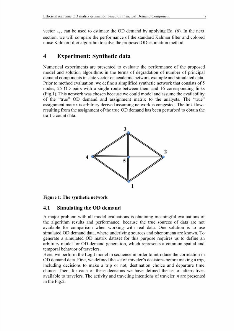
4 Experiment: Synthetic data Numerical experiments are presented to evaluate the performance of the proposedmodel and solution algorithms in the terms of degradation of number of principaldemand components in state vector on academic network example and simulated data.Prior to method evaluation, we define a simplified synthetic network that consists of 5nodes, 25 OD pairs with a single route between them and 16 corresponding links(Fig.1). This network was chosen because we could model and assume the availabilityof the “true” OD demand and assignment matrix to the analysts. The “true”assignment matrix is arbitrary derived assuming network is congested. The link flowsresulting from the assignment of the true OD demand has been perturbed to obtain the

traffic count data.

Figure 1: The synthetic network

4.1 Simulating the OD demand

A major problem with all model evaluations is obtaining meaningful evaluations ofthe algorithm results and performance, because the true sources of data are notavailable for comparison when working with real data. One solution is to use

simulated OD demand data, where underlying sources and phenomena are known. Togenerate a simulated OD matrix dataset for this purpose requires us to define anarbitrary model for OD demand generation, which represents a common spatial andtemporal behavior of travelers.Here, we perform the Logit model in sequence in order to introduce the correlation inOD demand data. First, we defined the set of traveler’s decisions before making a trip,including decisions to make a trip or not, destination choice and departure timechoice. Then, for each of these decisions we have defined the set of alternativesavailable to travelers. The activity and traveling intentions of traveler n are presentedin the Fig.2.

8/13/2019 Djukic 2012



Figure 2: The set of decisions and alternatives for traveler

The main principle of this model is that a large number of simulations are performed

for varying model inputs, reflecting the variability’s in the travelers behavior andconsequently in OD demand based on Monte Carlo simulations. Subsequently, wegenerate 1000 observations, each being a realization of the 25-dimensional ODdemand vector. Each generated OD demand vector without nonzero OD flows isstored in OD demand matrix X where each row represents one observation of ODdemand.

4.2 The model performance

To examine the effect of degradation of the number of principal demand componentsin state vector, we applied the PCA on the OD demand data matrix X . Once we

perform the PCA, we obtain the set of eigenvectors ei

for i = 1,2,...,20 and eigenvalues

! i for i =1,2,...,20 .

We have seen that we can use eigenvalues to explore the data reduction potential, forinstance by considering the total (cumulative) percentage of total variation explained(e.g. 95%), Fig.3. We can observe that the 90% of the variance of the data is captured

by first 5 eigenvectors.

1 2 3 4 5 6 7 8 9 100

10

20

30

40

50

60

70

80

90

100

Principal Component

V a r i a n c e E x p l a i n e d

( % )

0%

10%

20%

30%

40%

50%

60%

70%

80%

90%

100%

Figure 3: Cumulative percentage of total variation explained by eigenvalues

8/13/2019 Djukic 2012



We have performed the experiments such that in every experiment run we omit theone state variable (principal demand component) from the state vector. Since the

principal demand components in the state vector are arranged in decreasing order ofan eigenvalues, in every experiment run we remove the principal demand componentthat captures the lowest variance. In every experiment, we have performed the 1000

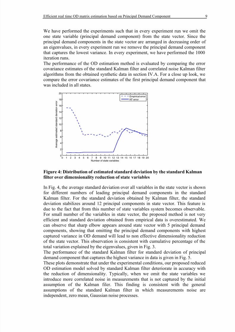
iteration runs.The performance of the OD estimation method is evaluated by comparing the errorcovariance estimates of the standard Kalman filter and correlated noise Kalman filteralgorithms from the obtained synthetic data in section IV.A. For a close up look, wecompare the error covariance estimates of the first principal demand component thatwas included in all states.

0 1 2 3 4 5 6 7 8 9 10 11 12 13 14 15 16 17 18 19 200

2

4

6

8

10

12

14

16

18

20

Number of state variables

A v e r a g e e s t i m a t e d s t a n d a r d d

e v i a t i o n e r r o r

Empirical error

KF error

Figure 4: Distribution of estimated standard deviation by the standard Kalman

filter over dimensionality reduction of state variables

In Fig. 4, the average standard deviation over all variables in the state vector is shownfor different numbers of leading principal demand components in the standardKalman filter. For the standard deviation obtained by Kalman filter, the standarddeviation stabilizes around 12 principal components in state vector. This feature isdue to the fact that from this number of state variables system becomes observable.For small number of the variables in state vector, the proposed method is not veryefficient and standard deviation obtained from empirical data is overestimated. Wecan observe that sharp elbow appears around state vector with 5 principal demand

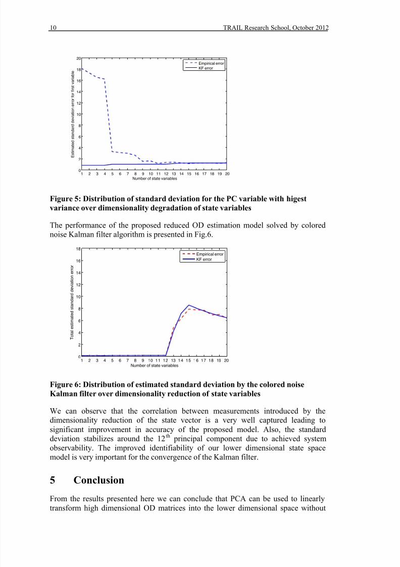
components, showing that omitting the principal demand components with highestcaptured variance in OD demand will lead to non effective dimensionality reductionof the state vector. This observation is consistent with cumulative percentage of thetotal variation explained by the eigenvalues, given in Fig. 3.The performance of the standard Kalman filter for standard deviation of principaldemand component that captures the highest variance in data is given in Fig. 5.These plots demonstrate that under the experimental conditions, our proposed reducedOD estimation model solved by standard Kalman filter deteriorate in accuracy withthe reduction of dimensionality. Typically, when we omit the state variables weintroduce more correlated noise in measurements that is not captured by the initialassumption of the Kalman filer. This finding is consistent with the general

assumptions of the standard Kalman filter in which measurements noise areindependent, zero mean, Gaussian noise processes.

8/13/2019 Djukic 2012



1 2 3 4 5 6 7 8 9 10 11 12 13 14 15 16 17 18 19 200

2

4

6

8

10

12

14

16

18

20


E s t i m a t e d s t a n d a r d d e v i a t i o n e r r o r

f o r f i r s t v a r i a b l e

Empirical error

KF error

Figure 5: Distribution of standard deviation for the PC variable with higestvariance over dimensionality degradation of state variables

The performance of the proposed reduced OD estimation model solved by colorednoise Kalman filter algorithm is presented in Fig.6.

1 2 3 4 5 6 7 8 9 10 11 12 13 14 15 16 17 18 19 200

2

4

6

8

10

12

14

16

18


T o t a l e s t i m a t e d s t a n d a

r d d e v i a t i o n e r r o r

Empirical error

KF error

Figure 6: Distribution of estimated standard deviation by the colored noise

Kalman filter over dimensionality reduction of state variables

We can observe that the correlation between measurements introduced by thedimensionality reduction of the state vector is a very well captured leading tosignificant improvement in accuracy of the proposed model. Also, the standarddeviation stabilizes around the 12th principal component due to achieved systemobservability. The improved identifiability of our lower dimensional state spacemodel is very important for the convergence of the Kalman filter.

5 Conclusion

From the results presented here we can conclude that PCA can be used to linearlytransform high dimensional OD matrices into the lower dimensional space without

8/13/2019 Djukic 2012



significant loss of estimation accuracy. We have proposed a new OD estimationmethod that uses the eigenvectors and principal demand components as state variablesinstead of OD flows. These variables can be used to construct a state space model thatcan be solved with recursive solution approaches such as the Kalman filter.The proposed state space model, however, appears to be sensitive to the reduction of

the dimensionality due to the induced temporal measurement correlation. We haveexplored and derived an analytical solution for the so-called colored noise Kalmanfilter algorithm that accounts for temporal correlated measurement noise to avoid thislimitation.The presented results are still academic in nature, and must be interpreted as a proofof concept. More results in more realistic settings are part of current research toascertain that the method performs well in practice.

Acknowledgment

This research is partly funded by the COST Action TU0903 – MULTITUDE projectin collaboration with Delft University of Technology and KTH University.

References

Antoniou, C., M. Ben-Akiva, et al. (2004). "Incorporating Automated VehicleIdentification Data into Origin-Destination Estimation." Transportation ResearchRecord: Journal of the Transportation Research Board 1882(-1): 37-44.

Antoniou, C., M. Ben-Akiva, et al. (2006). "Dynamic traffic demand prediction usingconventional and emerging data sources." Intelligent Transport Systems, IEE

Proceedings 153(1): 97-104.Asakura, Y., E. Hato, et al. (2000). "Origin-destination matrices estimation modelusing automatic vehicle identification data and its application to the Han-Shinexpressway network." Transportation 27(4): 419-438.

Ashok, K., M. E. Ben-Akiva, et al. (1993). "Dynamic origin-destination matrixestimation and prediction for real-time traffic management systems." Transportationand traffic theory.

Barcelo, J., L. Montero, et al. (2010). "Travel Time Forecasting and Dynamic Origin-Destination Estimation for Freeways Based on Bluetooth Traffic Monitoring."Transportation Research Record: Journal of the Transportation Research Board2175(-1): 19-27.

Barcelo, J. e. a. (2010). "A Kalman-filter approach for dynamic OD estimation incorridors based on bluetooth and Wi-Fi data collection." 12th World Conference onTransportation Research WCTR.

Bierlaire, M. and F. Crittin (2004). "An Efficient Algorithm for Real-Time Estimationand Prediction of Dynamic OD Tables." OPERATIONS RESEARCH 52(1): 116-127.

Bryson, A. E. (2002). "Applied Linear Optimal Control." Cambridge UniversityPress, Cambridge, UK: pp. 310–312.

Bryson, A. E., and Henrikson, L. J., (1968). "Estimation Using Sampled DataContaining Sequentially Correlated Noise." J. Spacecr. Rockets 56(pp.662 - 665).

8/13/2019 Djukic 2012



Dixon, M. P. and L. R. Rilett (2005). "Population Origin--Destination EstimationUsing Automatic Vehicle Identification and Volume Data." Journal of TransportationEngineering 131(2): 75-82.

Flötteröd, G., and Bierlaire, M. (2009). "Improved estimation of travel demand fromtraffic counts by a new linearization of the network loading map." Proceedings of theEuropean Transport Conference (ETC), Netherlands.

Frederix, R., Viti, F., and Tampère, C.M.J. (2011). "A hierarchical approach fordynamic origin-destination matrix estimation on large-scale congested networks."Proceedings of the IEEE-ITSC 2011 conference Washington DC, USA.

Golub, G. and C. van Van Loan (1996). Matrix Computations (Johns Hopkins Studiesin Mathematical Sciences)(3rd Edition), The Johns Hopkins University Press.

Jolliffe, I. T. (2002). Principal Component Analysis, Springer.

Kalman, R. E. (1960). "A New Approach to Linear Filtering and PredictionProblems." Transactions of the ASME ‚Äì Journal of Basic Engineering(82 (SeriesD)): 35-45.

Kattan, L. and B. Abdulhai (2006). "Noniterative Approach to Dynamic TrafficOrigin-Destination Estimation with Parallel Evolutionary Algorithms." TransportationResearch Record: Journal of the Transportation Research Board 1964(-1): 201-210.

Lou, Y. and Y. Yin (2010). "A decomposition scheme for estimating dynamic origin– destination flows on actuation-controlled signalized arterials." TransportationResearch Part C: Emerging Technologies 18(5): 643-655.

Zhou, X. and H. S. Mahmassani (2007). "A structural state space model for real-timetraffic origin-destination demand estimation and prediction in a day-to-day learning

framework." Transportation Research Part B: Methodological 41(8): 823-840.

Documents

Djukic 2012