Divide and Rule or the Rule of the Divided?

Evidence from Africa∗

Stelios Michalopoulos

Brown University and Tufts University

Elias Papaioannou

Dartmouth College, NBER and CEPR

December 29, 2011

Abstract

We investigate the importance of contemporary country-level institutional structures

and local ethnic-specific pre-colonial institutions in shaping comparative regional develop-

ment in Africa. We utilize information on the spatial distribution of African ethnicities

before colonization and regional variation in contemporary economic performance, as prox-

ied by satellite light density at night. We exploit the fact that political boundaries across

the African landscape partitioned ethnic groups in different countries subjecting identical

cultures to different country-level institutions. Our regression discontinuity estimates re-

veal that differences in countrywide institutional arrangements across the national border

do not explain differences in economic performance within ethnic groups. In contrast, we

document a strong association between pre-colonial ethnic institutional traits and contem-

porary regional development. While this correlation does not necessarily identify a causal

relationship, this result obtains conditional on country fixed effects, controlling for other

ethnic traits and when we focus on pairs of contiguous ethnic homelands where groups with

a different degree of local institutions reside.

Keywords: Africa, Borders, Ethnicities, Development, Institutions, Regression Discon-

tinuity

JEL classification Numbers: O10, O40, O43, N17, Z10.

∗We would like to thank 4 referees and the Editor for their invaluable comments. We thank seminar par-ticipants at Dartmouth, Tufts, Oxford, Vienna, Brown, Harvard, Stanford, UC-Berkeley, UC-Davis, NYU,

AUEB, the CEPR Development Economics Workshop, the World Bank, the IMF, the NBER Political Econ-

omy Meetings, the NBER Summer Institute Meetings in Economic Growth and Income Distribution and the

Macroeconomy for valuable comments. We also benefited from discussions with Yannis Ioannides, Rafael La

Porta, Antonio Ciccone, Rob Johnson, Raphael Frank, Jim Feyrer, Ross Levine, Avner Greif, Jeremiah Dittmar,

David Weil, Sandip Sukhtankar, Quamrul Ashraf, Oded Galor, Ed Kutsoati, Pauline Grosjean, Enrico Perotti,

Pedro Dal Bó, Nathan Nunn, Raquel Fernandez, Jim Robinson, and Enrico Spolaore. We are particularly

thankful to Andy Zeitlin, Melissa Dell, Andei Shleifer, Nico Voigtländer, and Daron Acemoglu for detailed

comments and useful suggestions. We also thank Nathan Nunn for providing the digitized version of Mur-

dock’s Tribal Map of Africa. A Supplementary Appendix with additional sensitivity checks is available online

at: http://www.dartmouth.edu/~elias/ and http://sites.google.com/site/steliosecon/. All errors are our sole

responsibility.

0

1 Introduction

In recent years there has been a surge of empirical research on the determinants of African

and more generally global underdevelopment. The predominant institutional view suggests

that poorly performing national institutional structures, such as lack of constraints on the

executive, poor property rights protection, as well as inefficient legal and court systems are

the ultimate causes of underdevelopment (see Acemoglu, Johnson, and Robinson (2005) for a

review). This body of research puts an emphasis on the impact of colonization on contemporary

country-level institutions and in turn on economic development. Yet in the African context

many downplay the importance of colonial and contemporary institutional structures. Recent

works on weak and strong states emphasize the limited state capacity of most African states

and their inability to provide public goods, collect taxes, and enforce contracts (Acemoglu

(2005); Besley and Persson (2009, 2010)). The inability of African governments to broadcast

power outside the capital cities has led many influential African scholars to highlight the role

of pre-colonial, ethnic-specific institutional and cultural traits. This body of research argues

that the presence of the Europeans in Africa was (with some exceptions) quite limited both

regarding timing and location. As a result of the negligible penetration of Europeans in the

mainland and the poor network infrastructure that has endured after independence, it is local,

ethnic-level, rather than national, institutional structures, that shape African development

today (see Herbst (2000) for a summary of the arguments).

In this paper we contribute to the literature on the determinants of African develop-

ment tackling these two distinct, though interrelated, questions. First, do contemporaneous

nationwide institutions affect economic performance across regions once we account for hard-to-

observe ethnicity-specific traits, culture, and geography? Second, do pre-colonial institutional

ethnic characteristics correlate with regional development once we consider country-specific

attributes, like economic/institutional performance, and national policies?

In contrast to most previous works that have relied on cross-country data and meth-

ods, we tackle these questions exploiting within-country and within-ethnicity regional varia-

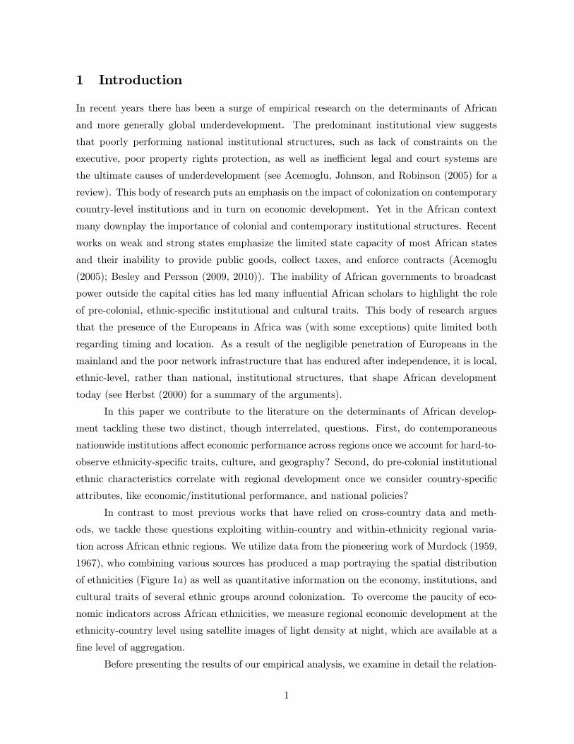
tion across African ethnic regions. We utilize data from the pioneering work of Murdock (1959,

1967), who combining various sources has produced a map portraying the spatial distribution

of ethnicities (Figure 1) as well as quantitative information on the economy, institutions, and

cultural traits of several ethnic groups around colonization. To overcome the paucity of eco-

nomic indicators across African ethnicities, we measure regional economic development at the

ethnicity-country level using satellite images of light density at night, which are available at a

fine level of aggregation.

Before presenting the results of our empirical analysis, we examine in detail the relation-

1

ship between satellite light density at night and economic well-being in Africa. We document

a strong positive correlation between light density and income per capita across African coun-

tries as well as infant mortality across administrative regions. Moreover, using micro-level data

from the Demographic and Health Surveys (DHS) we show that luminosity correlates strongly

with various proxy measures of development within countries. Most importantly, using micro-

data from the Afrobarometer surveys on access to public goods and education, we also show

that light density at night correlates with development proxies not only across regions within

countries, but also within ethnic homelands.

In the first part of our empirical analysis we examine the impact of contemporary na-

tional institutions on economic performance. In line with cross-country studies, we find a

positive correlation between rule of law (or control of corruption) and luminosity across ethnic

homelands. Yet due to omitted variables, reverse causation, and other potential sources of

endogeneity this correlation does not imply a causal relationship. To isolate the one-way effect

of contemporaneous institutions on regional development we exploit differences in country-level

institutional quality within ethnicities partitioned by national boundaries, as identified by in-

tersecting Murdock’s ethnolinguistic map with the 2000 Digital Chart of the World (Figure

1).

Ü

Historical Boundaries of Ethnicities Before Colonization

Traditional Ethnic Homelands

Figure 1: Ethnic Boundaries

Ü

Historical Boundaries ofEthnicities Before Colonization and National Boundaries

Traditional Ethnic Homelands

Contemporary National Boundaries

Figure 1: Ethnic and Country Boundaries

The artificial design of African borders, which took place in European capitals in the

late 19th century (mainly in the Berlin Conference in 1884− 5 and subsequent treaties in the1890), well before independence and when Europeans had hardly settled in the regions whose

2

borders were designing, offers a nice (quasi)-experimental setting to address this question.1

The drawing of colonial boundaries partitioned in the eve of African independence more than

200 ethnic groups across different countries. Taking advantage of this historical accident, we

compare economic performance in regions belonging to the historical homeland of the same

ethnic group, but are subject to different contemporary national institutions. Our approach

allows us to account for differences in geography, the disease environment, and other ecolog-

ical features. Moreover, by comparing development across border regions that belong to the

historical homeland of the same ethnic group (see Figures 2− 2 for examples), allows us toalso neutralize biases coming from cultural and other ethnic-specific differences. Our results

show that there is no systematic relationship between countrywide differences in institutions

and regional economic performance, as reflected in satellite images of light density at night,

within partitioned ethnicities in Africa. This pattern obtains both when the unit of analysis

is an ethnic partition and when we take advantage of the finer structure of the luminosity

data to construct multiple observations within each ethnic partition and perform a traditional

regression discontinuity (RD) analysis.

Figure 2 Figure 2

Figure 2 Figure 2

We obtain similar results when we perform our analysis in a sub-sample of partitioned

1There is no ambiguity among African scholars and historians that almost all African borders were artificially

drawn. See Asiwaju (1985) for examples and Michalopoulos and Papaioannou (2011) for additional references

on the artificial drawing of borders in Africa.

3

ethnic homelands where we have micro-level data from the Afrobarometer surveys on electrifica-

tion, access to clean water, access to a sewage system, and education. While in the cross section

there is a positive correlation between national institutional quality and these proxy measures

of development, the correlation becomes zero once we focus on within-ethnicity differences in

institutional quality across the border.

In the second part of our empirical investigation, we turn our focus on the economic

impact of pre-colonial ethnic institutions. Our analysis shows that political complexity at the

ethnicity level, before the advent of European colonizers, correlates significantly with contempo-

rary regional development, even when we account for national policies and other country-specific

features. This correlation does not necessarily imply a causal relationship, because one cannot

rule out the possibility that other ethnic characteristics and hard-to-account-for factors drive

the association between pre-colonial ethnic institutional traits and development. Yet the pos-

itive association between ethnic institutions and luminosity prevails numerous permutations.

First, it is robust to an array of controls related to the disease environment, land endowments,

and natural resources. Second, regressing luminosity on a variety of alternative pre-colonial

ethnicity-specific economic and cultural traits reported by Murdock (1967), we find that po-

litical centralization is the only robust correlate of regional economic development. Third, the

positive correlation between ethnic historical political complexity and regional development

is strong within pairs of adjacent ethnic homelands where groups with different pre-colonial

institutions reside. The uncovered pattern obtains both when the unit of analysis is an ethnic

homeland and when we exploit the finer structure of the luminosity data to obtain multiple

observations (pixels) for each ethnic homeland and conduct a regression discontinuity analysis.

Thus, although we do not have random assignment in ethnic institutions, the results

clearly point out that traits manifested in differences in the pre-colonial institutional legacy

of each ethnic group matter for contemporary African development. To get an idea of the

relative magnitudes the implied economic effect of pre-colonial ethnic institutions on regional

development is on average three times the implied (statistically insignificant) effect of national

institutions.

Related Literature Our research nests and advances over many strands of literature

that examine the historical roots of economic development in Africa.

First, an influential body of research asserts that through persistence, the institutions

that European powers established in the eve of colonization are the deep roots of contemporary

development. While there is ambiguity on the exact mechanisms via which colonization affected

African (and more generally non-European) development, there is an agreement that the type

4

of colonization and the identity of the colonizer had long-lasting effects on institutional quality

(e.g. La Porta et al. (1997, 1998, 1999); Acemoglu et al. (2001, 2002, 2005); Feyrer and

Sacerdote (2009)). Yet in spite of the ingenious instrumental variables identification schemes

employed in the cross-country literature, omitted variables and heterogeneity are always major

concerns (e.g. Glaeser et al. (2004), La Porta et al. (2008), Nunn (2009)). The micro approach

of our study enables us to overcome problems inherent to the cross-country framework adding

to a vibrant body of research that examines the within-country impact of historical institutions

(e.g. Banerjee and Iyer (2005); Huillery (2009); Iyer (2010); Acemoglu and Dell (2010) and

Gennaioli et al. (2011)).

Second, our identification scheme on the impact of national institutions explores disconti-

nuities across the border within partitioned ethnicities. As such our work relates to case studies

that examine the effect of national policies at the border. In an early contribution Miguel (2004)

compares public policies in health and education across the Kenya-Tanzania border to examine

the effect of Tanzanian nation-building policies. Using a similar to ours methodology, Bubb

(2009) investigates how differences in de jure property rights between Ghana and Ivory Coast

affect development in border areas. He finds that, despite large differences in de jure property

rights between the two countries, there are no differences in de facto property rights across the

border. Berger (2009) and Arbesu (2011) explore discontinuities across administrative colonial

boundaries within Nigeria to study the long-run effects of the different colonial tax systems.

The political science literature also investigates with case studies the impact of national policies

at the border. For example, Miles (1994) studies the development of the Hausa after their par-

titioning (at the Niger-Nigeria border), documenting that different French and British policies

(mainly on the role of local chiefs) endured after independence and had long-lasting effects.

Posner (2005) examines ethnic policies in Zambia and associates them with national represen-

tation. Our study, rather than focusing on the effect of national policies across a particular

border or within a single partitioned ethnic group, combines satellite light density images with

Murdock’s ethnolinguistic map to examine in a systematic way the effect of national institutions

on development across all of Africa’s partitioned ethnicities.

Third, our findings advance the literature on the role of pre-colonial, institutional and

cultural features in African development (Fortes and Evans-Pritchard (1940), Schapera (1967),

Stevenson (1968), Goody (1971), Bates (1983), Robinson (2002), Boone (2003), Englebert

(2009); see Herbst (2000) for an overview). This literature argues that ethnic groups had

marked differences in political centralization, land rights, and the power of local chiefs, among

others. As colonizers did not expand their power in remote areas far from the capital cities

and the coastline, such local institutions were preserved and were instrumental during the half-

5

century period of colonial rule (roughly 1890− 1940).2 Along the same lines, Mamdani (1996)argues that the indirect rule of the Europeans, if anything, increased the role of local chiefs

during the colonial era. Moreover, several African case studies stress the ongoing crucial role

of ethnic institutions and traditions (Englebert (2000); Miguel and Gugerty (2005); Franck

and Rainer (2009); Glennerster, Miguel, and Rothenberg (2010)). For example, in an early

contribution Douglas (1962) compares development between the neighboring groups of Lele

and Bushong in the Democratic Republic of Congo providing evidence that the two ethnicities

have different local institutions manifested in their different levels of development.

The African historiography has proposed various channels via which ethnic institutions

matter today. Herbst (2000) and Boone (2003) argue that in centralized societies there is a

high degree of political accountability of local chiefs. Others argue that centralized societies

were quicker in adopting growth-enhancing Western technologies and habits, because the col-

onizers collaborated more strongly with politically complex ethnic groups with strong chiefs

(Schapera (1967, 1970)). Herbst (2000) emphasizes the role of ethnic class stratification and

political centralization in establishing well-defined and secure land rights (see also Goldstein

and Udry (2008)). Furthermore, complex tribal societies with strong political institutions seem

to have been more successful in getting concessions both from colonial powers and from national

governments after independence.3

We improve upon this body of research showing that pre-colonial institutions are posi-

tively and systematically linked to regional development even when we control for local geogra-

phy and country-specific attributes. Accounting for common-to-all-ethnicities country factors

is central, as Gennaioli and Rainer (2006, 2007) show a positive cross-country correlation be-

tween pre-colonial centralization and current measures of institutional development. Moreover,

controlling for geography is important as studies on African institutional development argue

that pre-colonial political centralization was driven by land’s suitability for agriculture and

population density (e.g. Bates (1981); Fenske (2009)). Although our results do not necessarily

identify causal effects, they offer support to those emphasizing the importance of pre-colonial,

ethnicity-specific institutions in current times. In this regard our findings are in line with recent

empirical studies showing that historically determined socioeconomic and political factors have

persistent effects on comparative development (examples include the forced labor practices of

Spanish colonizers in Peru (Dell (2010)); the formation of city-states in Italy during the Middle

Ages (Guiso, Sapienza, and Zingales (2008)); 19th century inequality in Colombia (Acemoglu,

2For example, Acemoglu, Johnson, and Robinson (2003) partly attribute the economic success of Botswana

to the limited impact of colonization and the inclusive character of pre-colonial ethnic institutions.3Mamdani (1996), nevertheless, differs in his assessment on the beneficial contemporary role of hierarchical

pre-colonial structures arguing that the legacy of indirect rule in Africa through traditional chiefs was a basis

for post-independence poor institutional and economic performance.

6

Bautista, Querubin, and Robinson (2008)); the type of colonization and early inequality in

Brazil (Naritomi, Soares, and Assunção (2009)).

Moreover, the uncovered evidence on the limited role of national institutions on regional

development relates to works on state capacity (e.g. Tilly (1985); Migdal (1988); Acemoglu

(2005); Besley and Persson (2009, 2010); Acemoglu, Ticchi, and Vindigni (2011)) that em-

phasize the inability of weak states to broadcast power. Likewise, the finding that the positive

correlation between national institutions and regional development weakens in border areas has

implications for the literature on optimal state formation (e.g. Alesina and Spolaore (2003);

Spolaore and Wacziarg (2005)). Finally, this study contributes to a large body of work on the

historical causes of contemporary African development. Nunn (2008) stresses the importance

of the slave trade, while Englebert, Tarango, and Carter (2002), Alesina, Easterly, and Ma-

tuszeski (2011) and Michalopoulos and Papaioannou (2011) show a significant negative impact

on economic development from the improper colonial border design.

Paper Structure In the next section we first discuss the luminosity data and report

results from our cross-validation analysis examining the relationship between satellite light den-

sity and economic well being at various levels of aggregation (across countries, within countries

and within ethnic groups). Second, we present the pre-colonial ethnic institutional measures.

Third, we lay out the empirical specification and discuss estimation and inference. In section 3

we report our results on the effect of contemporary national institutions on regional develop-

ment. Section 4 presents our findings on the role of pre-colonial ethnic institutions in shaping

ethnic economic performance. Section 5 concludes.

2 Data and Identification

2.1 Data on partitioning

The starting point in compiling our dataset is George Peter Murdock’s (1959) Ethnolinguistic

map that portrays the spatial distribution of ethnicities across Africa around the European

colonization in the mid/late 19 century. Murdock’s map (reproduced in Figure 1) includes

843 tribal areas (the mapped groups correspond roughly to levels 7 − 8 of the Ethnologue’slanguage family tree); 8 areas are classified as uninhabited upon colonization and are therefore

not considered in our analysis. We also eliminate the Guanche, a small group in the Madeira

islands that is currently part of Portugal. One may wonder how much the spatial distribution of

ethnicities across the continent has changed over the past 100− 150 years. Reassuringly, usingindividual data from the Afrobarometer Nunn andWantchekon (2011) show a strong correlation

(around 055) between the location of the respondents in 2005 and the historical homeland of

7

their ethnicity as identified in Murdock’s (1959) map. In the same vein, Glennerster, Miguel,

and Rothenberg (2010) document in Sierra Leone that after the massive displacement of the

1991− 2002 civil war there has been a systematic movement of individuals towards the areasof their ethnic group’s historical homeland.

We project on top of Murdock’s ethnolinguistic map the 2000 Digital Chart of the World

(Figure 1) that portrays contemporary national boundaries yielding 1 247 country-tribe obser-

vations. This allows us to identify in a systematic way partitioned ethnicities. Appendix Table

12 lists split groups, defined as groups where at least 10% of their historical homeland belongs

to more than one contemporary state. In the empirical analysis we focus on partitions of at

least 100 square kilometers as tiny partitions are most likely due to the lack of precision in the

underlying mapping of ethnicities. Our procedure identifies 526 partitions that belong to 227

ethnic groups. For example, the Maasai have been partitioned between Kenya and Tanzania

(shares 62% and 38% respectively), the Anyi between Ghana and the Ivory Coast (shares 58%

and 42%), and the Chewa between Mozambique (50%), Malawi (34%), and Zimbabwe (16%).

We also checked whether our codification of partitioned ethnicities is in line with Asiwaju

(1985), who provides the only systematic codification (to our knowledge) of split ethnicities in

Africa. Our strategy identifies almost all ethnic groups that Asiwaju (1985) lists as partitioned.

Our procedure reveals that the median country in Africa has 43% of its population belonging

to partitioned ethnicities. This estimate is of the same order of magnitude to that of Englebert

et al. (2002) and Alesina et al. (2011), who using alternative sources and techniques estimate

that on average 40% of the African population comes from partitioned ethnic groups.

2.2 Satellite Light Density at Night

The nature of our study requires detailed data on economic development at the grid level.

To the best of our knowledge, geocoded high-resolution measures of economic development

spanning all Africa are not readily available. To overcome this issue we use satellite data on

light density at night to proxy for local economic activity.

The luminosity data come from the Defense Meteorological Satellite Program’s Opera-

tional Linescan System (DMSP-OLS) that reports images of the earth at night captured from

20 : 00 to 21 : 30 local time. The satellite detects lights from human settlements, fires, gas

flares, heavily lit fishing boats, lightning, and the aurora. The measure is a six-bit digital num-

ber (ranging from 0 to 63) calculated for every 30-second area pixel (approximately 1 square

kilometer). The resulting annual composite images are created by overlaying all images cap-

tured during a calendar year, dropping images where lights are shrouded by cloud cover or

overpowered by the aurora or solar glare (near the poles), and removing ephemeral lights like

8

fires, lightning and other noise. The result is a series of global images of time-stable night

lights. Using these data we construct average light density per square kilometer for 2007 and

2008 averaging across pixels at the desired level of aggregation.

This high-resolution dataset makes the data uniquely suited to spatial analyses of eco-

nomic development in Africa for several reasons. First, most African countries have low quality

income statistics, even at the national level (for example, the codebook of the Penn World Ta-

bles assigns the lowest scores on data quality to all African countries). Second, we lack data on

regional income or value added for most African countries. And while there are some regional

proxies of poverty and health, these data do not map to our unit of analysis and they are not

usually comparable across countries (as survey methods differ).

The use of luminosity data as a proxy for development builds on the recent contribution

by Henderson, Storeygard, and Weil (2011) and previous works (e.g. Elvidge, Baugh, Kihn,

Kroehl, and Davis (1997); Doll, Muller, and Morley (2006); Sutton, Elvidge, and Ghosh (2007))

showing that light density at night is a good proxy of economic activity. These studies establish

a strong within-country correlation between light density at night and GDP levels and growth

rates. There is also a strong association between luminosity and access to electricity and public

goods provision, especially across low income countries (see Elvidge, Baugh, Kihn, Kroehl, and

Davis (1997) and Min (2008)). Even Chen and Nordhaus (2010), who emphasize some problems

of the satellite image data, argue that luminosity can be quite useful for regional analysis in

war-prone countries with poor quality income data.

Satellite data on lights are subject to saturation and blooming. Saturation occurs at a

level of light similar to that in the urban centers of rich countries and results in top-coded values.

Blooming occurs because lights tend to appear larger than they actually are, especially for

bright lights over water and snow. These issues, however, are less pressing within Africa. First,

there are very few instances of top-coding (out of the 30 457 572 pixels of light density only

000017% are top-coded). Second, since luminosity is quite low across African regions, blooming

(bleeding) that occurs due to the diffusion of lights is not a major problem. Additionally,

to account for overglow over water, area under water and distance to the sea are standard

geographic controls in our regressions.

Variation in satellite light density across countries and regions may arise because of: (i)

cultural differences in use of lights; (ii) geographic differences; (iii) the composition of income

between consumption and investment; (iv) the division of economic activity between night and

day (or across sectors), and (v) the satellite used. By including country and ethnicity fixed

effects, and conditioning on a rich set of climatic and geographic control variables, we account

for these problems.

9

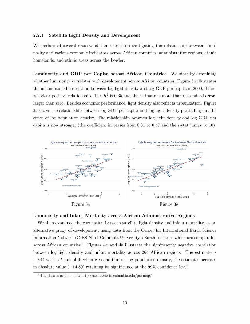
2.2.1 Satellite Light Density and Development

We performed several cross-validation exercises investigating the relationship between lumi-

nosity and various economic indicators across African countries, administrative regions, ethnic

homelands, and ethnic areas across the border.

Luminosity and GDP per Capita across African Countries We start by examining

whether luminosity correlates with development across African countries. Figure 3 illustrates

the unconditional correlation between log light density and log GDP per capita in 2000. There

is a clear positive relationship. The 2 is 035 and the estimate is more than 6 standard errors

larger than zero. Besides economic performance, light density also reflects urbanization. Figure

3 shows the relationship between log GDP per capita and log light density partialling out the

effect of log population density. The relationship between log light density and log GDP per

capita is now stronger (the coefficient increases from 031 to 047 and the t-stat jumps to 10).

MoroccoLibya

Angola

Botswana

Benin

Burundi

Chad

Congo (Democratic Republic of the)

Cameroon

ComorosCentral African Republic

Djibouti

Egypt

Equatorial Guinea

Ethiopia

The Gambia

Gabon

GhanaCote D'Ivoire

Kenya

Liberia

Lesotho

Madagascar Malawi

Mali

Mozambique

Niger

Nigeria

Guinea-Bissau

Rwanda

South Africa

Sierra Leone

SomaliaSudan

Togo

Tunisia

Tanzania

UgandaBurkina Faso

Swaziland

Zambia

Algeria

Republic of Congo

Guinea

Senegal

Mauritania

Zimbabwe

Namibia

56

78

9Lo

g (G

DP

per

Ca

pita

in 2

000)

-6 -4 -2 0 2Log (Light Density in 2007-2008)

Unconditional RelationshipLight Density and Income per Capita Across African Countries

Figure 3

Morocco

Libya

Angola

Botswana

Benin

Burundi

Chad

Congo (Democra tic Republic of the)

Cameroon

Comoros

Central African Republic

Djibouti

Egypt

Equatorial Guinea

Ethiopia

The Gambia

Gabon

GhanaCote D'Ivoi re

Kenya

Liberia

Lesotho

MadagascarMalawi

Mali

Mozambique

Niger

Nigeria

Guinea-Bissau

Rwanda

South Africa

Sierra Leone

SomaliaSudan

Togo

Tunisia

Tanzania

Uganda Burkina Faso

Swazi land

Zambia

Algeria

Republi c of Congo

Guinea

Senegal

Mauritania

Zimbabwe

Namibia

-2-1

01

2

Log

(GD

P p

er

Cap

ita in

200

0)

-2 -1 0 1 2 3

Log (Light Density in 2007-2008)

Conditional on Population Density

Light Density and Income per Capita Across African Countries

Figure 3

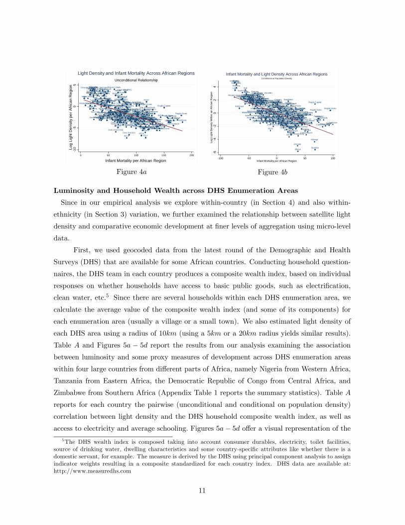
Luminosity and Infant Mortality across African Administrative Regions

We then examined the correlation between satellite light density and infant mortality, as an

alternative proxy of development, using data from the Center for International Earth Science

Information Network (CIESIN) of Columbia University’s Earth Institute which are comparable

across African countries.4 Figures 4 and 4 illustrate the significantly negative correlation

between log light density and infant mortality across 264 African regions. The estimate is

−944 with a t-stat of 9; when we condition on log population density, the estimate increasesin absolute value (−1489) retaining its significance at the 99% confidence level.

4The data is available at: http://sedac.ciesin.columbia.edu/povmap/

10

Região Sul

Congo

Região Centro SulNorth-Western

Região Capital

Região Oeste

Centra lRegião Norte

Congo, Dem. Rep. OfWestern

Northwest

Northeast

Região Este

BurundiButare

Kigali Rurale

Lake

Cyangugu

Kibungo

Borgou

Tillaberi (inc. Niamey)Plateaux

Savanes

Central

OuemeMarities

Dosso

Kara

North West

East

Zou

Atacora

Mono

Centrale

South WestAtlantique

Segou

Central/South & OuagadougouUpper East

Northern

Gao/Kidal/Tombouctou

Côte d'Ivoire

Mopti

SikassoWest

North

Upper West

Ghanzi

South

North West

Matabeleland North

Northe rn ProvinceNorth East

CentralMatabeleland South

SouthernSouthern

Northern Cape

Kgalagadi

South East

Kweneng

Kgat leng

North West

Bangui

RS V

S.Darfur

Centra l, South, & East

RS II

W. Darfur

RS I

North/ Extreme north/Adamaoua

RS III

Chad

RS IV

Upper GuineaForest Guinea

Western

Brong-Ahafo

Liberia

North East

Nord

Northwest & southwest

West & littoral

South East

Equatorial Guinea

Luapula

Cen tral

Copperbelt

Sud

Est

Moheli

Grande Comore

Anjouan

Cape Verde

Affa r

Debubawi Keih Bahri

Djibouti

North/West

Sud

Tunisia

Zone Nord (G3)

Oriental

OuestCentre

Tahoua/Agadez

Sud

Centre-SudLibya

Est

Occupied Palestinian Territories

Israel

GharbiaMenoufia

Matrouh

Suhag

IsmailiaBehera

DakahliaDamietta

AswanSuez

Fayoum

Giza

North Sina

SharkiaKalyoubia

Port-Said

South Sina

Nile River

Cairo

Northe rn

New Valley

Menia

Beni-SuetKafr El-Sh

Assyout

Red Sea

AlexandriaQuena

Red Sea

Maekel

Gash-BarkaSemenawi Keih BahriAnseba Gadaref

TigrayKassala

DebubSinnar

Somali

OromiyaEastern

Gambela

Harari

Dire Dawa

Rift Valley

Addis

SNNP

Central/South

Amhara

North/EastNorth Eastern

Ben-Gumz

Blue Nile

Ouest (inc. Libreville)Eastern

Volta

AshantiCentral

Greater Accra

Lower Guinea

Conakry

Guinea-Bissau Sierra Leone

Central Guinea

Koulikoro (inc. Bamako)

Nord-EstKayes

SudMacCarthy Island

KerewanMansakonkoBasse

Centre

Banjul

Brikama

Coastal

Nairobi

Northern Highla ndsCoast

Western

Centra l

Eastern

Northern

Nyanza

N.Darfur

Eastern CapeFree State

KwaZulu Natal

Lesotho

Centre-NordTensift

Centre

Toamasina

MahajangaToliary

Antananarivo

Fianarantsoa

Antsiranana

Zone Centre (G4)

Zone Fleuve (G2)

Zone Sud (G1)

MasvingoGaza

Eastern

Niassa

Central

Southern

Nampula

Mashonaland East

Tete

Cabo Delgado

Sofa laInhambane

LusakaMaputo province

Manica

South

Mashonaland CentralManicaland

Maputo Cidade

Zambezia

SwazilandMpumalanga

North

Nouakchott

Mauritius

Southern Highlands Northern

Zinda/Dif fa

Maradi

Umutara

Ruhengeri

Western

ByumbaKibuye

Kigali Ville (PVK)

Gitarama

Gisenyi

S.Kordofan

White Nile

Khartoum

Gazira

W. Kordofan

N.Kordofan

Ouest

Sao Tome and Principe

Seychelles

Central

Central

Gauteng

Western Cape

Mashonaland WestMidlands

BulawayoHarare

-10

-50

5L

og

Lig

ht D

en

sity

pe

r A

fric

an

Re

gion

0 50 100 150 200

Infant Mortality per African Region

Unconditional Relationship

Light Density and Infant Mortality Across African Regions

Figure 4

Central

Congo, Dem. Rep. Of

Região Capital

Região OesteRegião Centro SulRegião EsteNorth-Western

NortheastNorthwest

Região SulWestern

Região Norte

Congo

Cyangugu

Butare

Burundi

Kibungo

Kigali Rurale

Lake

Mono

Atlantique

Zou

Marities

Borgou

Central Tillaberi (inc. Niamey)

South West

AtacoraSavanes Dosso

Oueme

North West

CentralePlateauxKara

EastMopti

Upper EastGao/Kidal/Tombouctou

Upper West Segou

North

Sikasso

Northern

Côte d'Ivoire

Central/South & Ouagadougou

West

South EastSouthNorth EastNorthern Cape

Southern

KgalagadiNorth West

Ghanzi

Matabeleland North

CentralKweneng

Matabeleland South

Northern Province

KgatlengNorth WestSouthern

RS V

RS II

RS IS.Darfur

RS IV

Central, South, & East

Chad

RS III

North/ Extreme north/Adamaoua

Bangui

W. Darfur

Western

Brong-Ahafo

LiberiaUpper Guinea

Forest Guinea

Northwest & southwest

South East

North East

West & littoral

Equatorial Guinea

Nord

Luapula

Copperbelt

Central

Sud

Est

Anjouan

Grande Comore

Moheli

Cape Verde

North/West

Debubawi Keih Bahri

Djibouti

Affar

Tunisia

CentreEst

Sud

Zone Nord (G3)

Libya

OuestOriental

Tahoua/Agadez

SudCentre-Sud

Ismailia

Red Sea

New Valley

Assyout

Port-Said

North Sina

Giza

Red Sea

Kafr El-ShKalyoubia

DamiettaDakahlia

QuenaFayoumNorthern

Alexandria

Aswan

Menoufia

Cairo

Beni-Suet

South Sina

Nile River

Menia

Gharbia

Suez

SharkiaSuhagBehera

Matrouh

Anseba

Maekel

Gadaref

Kassala

TigrayDebub

Gash-BarkaSemenawi Keih Bahri

Spain

Nord-Ouest

Addis

Rift Valley

North EasternSomali

Oromiya

Harari

Gambela

Dire Dawa

Amhara

Ben-Gumz

SNNPNorth/East

Blue Nile

Central/South

Eastern

Sinnar

Ouest (inc. Libreville)

CentralAshanti

Greater Accra

EasternVolta

Guinea-Bissau

Lower Guinea

Central Guinea

Koulikoro (inc. Bamako)

Sierra Leone

Conakry

Sud

Nord-EstKayes

MacCarthy Island

Brikama

Kerewan

Banjul

Mansakonko

Centre

Basse

Coastal

Nyanza

Nairobi

Northern

Northern Highlands

Central Coast

WesternEastern

N.Darfur

Eastern CapeKwaZulu Natal

Lesotho

Free State

CentreTensiftCentre-Nord

Antananarivo

Mahajanga

Antsiranana

Toliary

Fianarantsoa

ToamasinaZone Sud (G1)

Zone Centre (G4)

Zone Fleuve (G2)

Sofala

Cabo DelgadoZambezia

Mashonaland Central

Manicaland

SouthInhambane

Masvingo

Southern

Eastern

Central

Niassa

Mashonaland East

Swaziland

Gaza

Mpumalanga

Lusaka

TeteNampula

Maputo Cidade

Manica

Maputo province

North

Nouakchott

Mauritius

Northern

Southern Highlands MaradiZinda/Diffa

Western

Umutara

Gitarama

Kibuye

Kigali Ville (PVK)

Gisenyi

Ruhengeri

Byumba

W. Kordofan

N.Kordofan

White Nile

KhartoumGazira

S.Kordofan

OuestSao Tome and Principe

Seychelles

Central

Central

Western Cape

Gauteng

Mashonaland West

Midlands

Harare

Bulawayo

-6-4

-20

24

Lo

g L

ight

De

nsi

ty W

ithin

an

Afr

ican

Re

gio

n

-100 -50 0 50 100Infant Mortality per African Region

Conditional on Population Density

Infant Mortality and Light Density Across African Regions

Figure 4

Luminosity and Household Wealth across DHS Enumeration Areas

Since in our empirical analysis we explore within-country (in Section 4) and also within-

ethnicity (in Section 3) variation, we further examined the relationship between satellite light

density and comparative economic development at finer levels of aggregation using micro-level

data.

First, we used geocoded data from the latest round of the Demographic and Health

Surveys (DHS) that are available for some African countries. Conducting household question-

naires, the DHS team in each country produces a composite wealth index, based on individual

responses on whether households have access to basic public goods, such as electrification,

clean water, etc.5 Since there are several households within each DHS enumeration area, we

calculate the average value of the composite wealth index (and some of its components) for

each enumeration area (usually a village or a small town). We also estimated light density of

each DHS area using a radius of 10 (using a 5 or a 20 radius yields similar results).

Table and Figures 5 − 5 report the results from our analysis examining the association

between luminosity and some proxy measures of development across DHS enumeration areas

within four large countries from different parts of Africa, namely Nigeria from Western Africa,

Tanzania from Eastern Africa, the Democratic Republic of Congo from Central Africa, and

Zimbabwe from Southern Africa (Appendix Table 1 reports the summary statistics). Table

reports for each country the pairwise (unconditional and conditional on population density)

correlation between light density and the DHS household composite wealth index, as well as

access to electricity and average schooling. Figures 5− 5 offer a visual representation of the5The DHS wealth index is composed taking into account consumer durables, electricity, toilet facilities,

source of drinking water, dwelling characteristics and some country-specific attributes like whether there is a

domestic servant, for example. The measure is derived by the DHS using principal component analysis to assign

indicator weights resulting in a composite standardized for each country index. DHS data are available at:

http://www.measuredhs.com

11

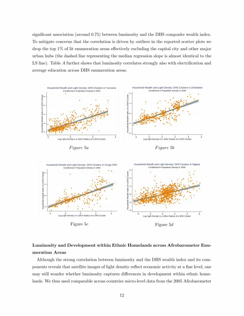
significant association (around 075) between luminosity and the DHS composite wealth index.

To mitigate concerns that the correlation is driven by outliers in the reported scatter plots we

drop the top 1% of lit enumeration areas effectively excluding the capital city and other major

urban hubs (the dashed line representing the median regression slope is almost identical to the

LS line). Table further shows that luminosity correlates strongly also with electrification and

average education across DHS enumeration areas.

-10

12

3H

ouse

hold

Wea

lth In

dex

of a

DH

S C

lust

er

-2 0 2 4Log Light Density in a 10km Radius of a DHS Cluster

Conditional in Population Density in 2000

Household Wealth and Light Density: DHS Clusters in Tanzania

-2-1

01

2H

ouse

hold

Wea

lth In

dex

of a

DH

S C

lust

er

-4 -2 0 2 4 6Log Light Density in a 10km Radius of a DHS Cluster

Conditional in Population Density in 2000

Household Wealth and Light Density: DHS Clusters in Zimbabwe

5 5

-10

12

Hou

seho

ld W

ealth

Inde

x o

f a D

HS

Clu

ster

-4 -2 0 2 4Log Light Density in a 10km Radius of a DHS Cluster

Conditional in Population Density in 2000

Household Wealth and Light Density: DHS Clusters in Congo DRC

Figure 5

-2-1

01

23

Hou

seho

ld W

ealth

Inde

x o

f a D

HS

Clu

ster

-4 -2 0 2 4 6Log Light Density in a 10km Radius of a DHS Cluster

Conditional in Population Density in 2000

Household Wealth and Light Density: DHS Clusters in Nigeria

Figure 5

Luminosity and Development within Ethnic Homelands across Afrobarometer Enu-

meration Areas

Although the strong correlation between luminosity and the DHS wealth index and its com-

ponents reveals that satellite images of light density reflect economic activity at a fine level, one

may still wonder whether luminosity captures differences in development within ethnic home-

lands. We thus used comparable across countries micro-level data from the 2005 Afrobarometer

12

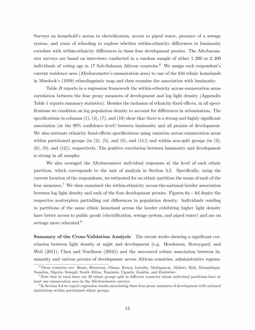
Surveys on household’s access to electrification, access to piped water, presence of a sewage

system, and years of schooling to explore whether within-ethnicity differences in luminosity

correlate with within-ethnicity differences in these four development proxies. The Afrobarom-

eter surveys are based on interviews conducted in a random sample of either 1 200 or 2 400

individuals of voting age in 17 Sub-Saharan African countries.6 We assign each respondent’s

current residence area (Afrobarometer’s enumeration area) to one of the 834 ethnic homelands

in Murdock’s (1959) ethnolinguistic map and then examine the association with luminosity.

Table reports in a regression framework the within-ethnicity across enumeration areas

correlation between the four proxy measures of development and log light density (Appendix

Table 1 reports summary statistics). Besides the inclusion of ethnicity fixed effects, in all speci-

fications we condition on log population density to account for differences in urbanization. The

specifications in columns (1), (4), (7), and (10) show that there is a strong and highly significant

association (at the 99% confidence level) between luminosity and all proxies of development.

We also estimate ethnicity fixed-effects specifications using variation across enumeration areas

within partitioned groups (in (2), (5), and (8), and (11)) and within non-split groups (in (3),

(6), (9), and (12)), respectively. The positive correlation between luminosity and development

is strong in all samples.

We also averaged the Afrobarometer individual responses at the level of each ethnic

partition, which corresponds to the unit of analysis in Section 32. Specifically, using the

current location of the respondents, we estimated for an ethnic partition the mean of each of the

four measures.7 We then examined the within-ethnicity across-the-national-border association

between log light density and each of the four development proxies. Figures 6− 6 depict therespective scatterplots partialling out differences in population density. Individuals residing

in partitions of the same ethnic homeland across the border exhibiting higher light density

have better access to public goods (electrification, sewage system, and piped water) and are on

average more educated.8

Summary of the Cross-Validation Analysis The recent works showing a significant cor-

relation between light density at night and development (e.g. Henderson, Storeygard, and

Weil (2011); Chen and Nordhaus (2010)) and the uncovered robust association between lu-

minosity and various proxies of development across African countries, administrative regions,

6These countries are: Benin, Botswana, Ghana, Kenya, Lesotho, Madagascar, Malawi, Mali, Mozambique,

Namibia, Nigeria, Senegal, South Africa, Tanzania, Uganda, Zambia, and Zimbabwe.7Note that in total there are 32 ethnic groups split in different countries whose individual partitions have at

least one enumeration area in the Afrobarometer surveys.8 In Section 34 we report regression results associating these four proxy measures of development with national

institutions within partitioned ethnic groups.

13

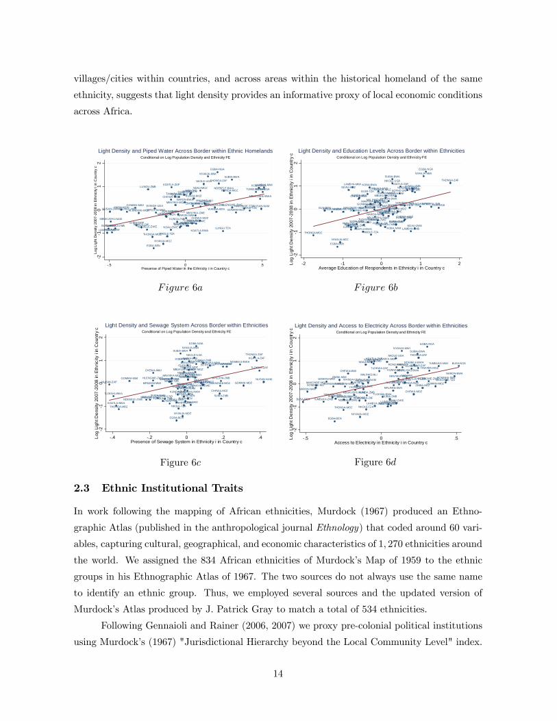
villages/cities within countries, and across areas within the historical homeland of the same

ethnicity, suggests that light density provides an informative proxy of local economic conditions

across Africa.

BUSA-BEN

BUSA-NGA

CHEWA-MWI

CHEWA-MOZ

EGBA-NGA

EGBA-BEN

GOMANI-MWI

GOMANI-MOZ

GUSII-TZA

GUSII-KEN

HLENGWE-ZWE

HLENGWE-MOZ

KGATLA-BWA

KGATLA-ZAF

KOBA-NAM

KOBA-BWA

KUNDA-MOZ

KUNDA-ZMB

LAMBYA-ZMB

LAMBYA-MWILUNGU-ZMB

LUNGU-TZA

MAKONDE-TZAMAKONDE-MOZ

MALINKE-SEN

MALINKE-MLIMANYIKA-MOZ

MANYIKA-ZWE

MASAI-TZAMASAI-KEN

MBUKUSHU-NAM

MBUKUSHU-BWA

MPEZENI-MWI

MPEZENI-ZMB

NARON-BWA

NARON-NAM

NDAU-MOZ

NDAU-ZWENDEBELE-ZWE

NDEBELE-BWA

NKOLE-UGA

NKOLE-TZA

NUSAN-NAMNUSAN-ZAF

NYANJA-MWI

NYANJA-MOZ

RONGA-MOZ

RONGA-ZAF

SONINKE-SEN

SONINKE-MLI

SOTHO-LSO

SOTHO-ZAF

SUBIA-BWA

SUBIA-ZMBSUBIA-NAM

TAWARA-MOZ

TAWARA-ZWE

THONGA-MOZ

THONGA-ZAF

TLOKWA-BWA

TLOKWA-ZAF

TUMBUKA-MWI

TUMBUKA-ZMB

WANGA-KENWANGA-UGA

XAM-LSO

XAM-ZAF

YAO-MOZ

YAO-MWIZIMBA-MWI

ZIMBA-MOZ

-2-1

01

2L

og

Lig

ht D

en

sity

200

7-2

00

8 in

Eth

nic

ity i

in C

oun

try

c

-.5 0 .5Presense of Piped Water in the Ethnicity i in Country c

Conditional on Log Population Density and Ethnicity FE

Light Density and Piped Water Across Border within Ethnic Homelands

BUSA-BEN

BUSA-NGA

CHEWA-MWI

CHEWA-MOZ

EGBA-NGA

EGBA-BEN

GOMANI-MWI

GOMANI-MOZGUN-NGA

GUN-BEN

GUSII-TZA

GUSII-KEN

HLENGWE-ZWE

HLENGWE-MOZ

KGATLA-BWA

KGATLA-ZAF

KOBA-NAM

KOBA-BWA

KUNDA-MOZ

KUNDA-ZMB

LAMBYA-ZMB

LAMBYA-MWILUNGU-ZMB

LUNGU-TZA

MAKONDE-TZAMAKONDE-MOZ

MALINKE-SEN

MALINKE-MLIMANYIKA-MOZ

MANYIKA-ZWE

MASAI-TZA MASAI-KEN

MBUKUSHU-NAM

MBUKUSHU-BWA

MPEZENI-MWI

MPEZENI-ZMB

NARON-BWA

NARON-NAM

NDAU-MOZ

NDAU-ZWENDEBELE-ZWE

NDEBELE-BWA

NKOLE-UGA

NKOLE-TZA

NUSAN-NAMNUSAN-ZAF

NYANJA-MWI

NYANJA-MOZ

RONGA-MOZ

RONGA-ZAF

SONINKE-SEN

SONINKE-MLI

SOTHO-LSO

SOTHO-ZAF

SUBIA-BWA

SUBIA-ZMBSUBIA-NAM

TAWARA-MOZ

TAWARA-ZWE

THONGA-MOZ

THONGA-ZAF

TLOKWA-BWA

TLOKWA-ZAF

TUMBUKA-MWI

TUMBUKA-ZMB

WANGA-KENWANGA-UGA

XAM-LSO

XAM-ZAF

YAO-MOZ

YAO-MWIZIMBA-MWI

ZIMBA-MOZ

-2-1

01

2L

og L

igh

t De

nsity

20

07-2

008

in E

thni

city

i in

Co

untr

y c

-2 -1 0 1 2Average Education of Respondents in Ethnicity i in Country c

Conditional on Log Population Density and Ethnicity FE

Light Density and Education Levels Across Border within Ethnicities

6 6

BUSA-BEN

BUSA-NGA

CHEWA-MWI

CHEWA-MOZ

EGBA-NGA

EGBA-BEN

GOMANI-MWI

GOMANI-MOZ

GUSII-TZA

GUSII-KEN

HLENGWE-ZWE

HLENGWE-MOZ

KGATLA-BWA

KGATLA-ZAF

KOBA-NAM

KOBA-BWA

KUNDA-MOZ

KUNDA-ZMB

LAMBYA-ZMB

LAMBYA-MWILUNGU-ZMB

LUNGU-TZA

MAKONDE-TZAMAKONDE-MOZ

MALINKE-SEN

MALINKE-MLIMANYIKA-MOZ

MANYIKA-ZWE

MASAI-TZA MASAI-KEN

MBUKUSHU-NAM

MBUKUSHU-BWA

MPEZENI-MWI

MPEZENI-ZMB

NARON-BWA

NARON-NAM

NDAU-MOZ

NDAU-ZWENDEBELE-ZWE

NDEBELE-BWA

NKOLE-UGA

NKOLE-TZA

NUSAN-NAMNUSAN-ZAF

NYANJA-MWI

NYANJA-MOZ

RONGA-MOZ

RONGA-ZAF

SONINKE-SEN

SONINKE-MLI

SOTHO-LSO

SOTHO-ZAF

SUBIA-BWA

SUBIA-ZMBSUBIA-NAM

TAWARA-MOZ

TAWARA-ZWE

THONGA-MOZ

THONGA-ZAF

TLOKWA-BWA

TLOKWA-ZAF

TUMBUKA-MWI

TUMBUKA-ZMB

WANGA-KENWANGA-UGA

XAM-LSO

XAM-ZAF

YAO-MOZ

YAO-MWIZIMBA-MWI

ZIMBA-MOZ

-2-1

01

2L

og L

igh

t De

nsity

20

07-2

008

in E

thni

city

i in

Co

untr

y c

-.4 -.2 0 .2 .4Presence of Sewage System in Ethnicity i in Country c

Conditional on Log Population Density and Ethnicity FE

Light Density and Sewage System Across Border within Ethnicities

Figure 6

BUSA-BEN

BUSA-NGA

CHEWA-MWI

CHEWA-MOZ

EGBA-NGA

EGBA-BEN

GOMANI-MWI

GOMANI-MOZGUN-NGA

GUN-BEN

GUSII-TZA

GUSII-KEN

HLENGWE-ZWE

HLENGWE-MOZ

KGATLA-BWA

KGATLA-ZAF

KOBA-NAM

KOBA-BWA

KUNDA-MOZ

KUNDA-ZMB

LAMBYA-ZMB

LAMBYA-MWILUNGU-ZMB

LUNGU-TZA

MAKONDE-TZAMAKONDE-MOZ

MALINKE-SEN

MALINKE-MLI MANYIKA-MOZ

MANYIKA-ZWE

MASAI-TZAMASAI-KEN

MBUKUSHU-NAM

MBUKUSHU-BWA

MPEZENI-MWI

MPEZENI-ZMB

NARON-BWA

NARON-NAM

NDAU-MOZ

NDAU-ZWENDEBELE-ZWE

NDEBELE-BWA

NKOLE-UGA

NKOLE-TZA

NUSAN-NAMNUSAN-ZAF

NYANJA-MWI

NYANJA-MOZ

RONGA-MOZ

RONGA-ZAF

SONINKE-SEN

SONINKE-MLI

SOTHO-LSO

SOTHO-ZAF

SUBIA-BWA

SUBIA-ZMBSUBIA-NAM

TAWARA-MOZ

TAWARA-ZWE

THONGA-MOZ

THONGA-ZAF

TLOKWA-BWA

TLOKWA-ZAF

TUMBUKA-MWI

TUMBUKA-ZMB

WANGA-KENWANGA-UGA

XAM-LSO

XAM-ZAF

YAO-MOZ

YAO-MWIZIMBA-MWI

ZIMBA-MOZ

-2-1

01

2L

og L

igh

t De

nsity

20

07-2

008

in E

thni

city

i in

Co

untr

y c

-.5 0 .5Access to Electricity in Ethnicity i in Country c

Conditional on Log Population Density and Ethnicity FE

Light Density and Access to Electricity Across Border within Ethnicities

Figure 6

2.3 Ethnic Institutional Traits

In work following the mapping of African ethnicities, Murdock (1967) produced an Ethno-

graphic Atlas (published in the anthropological journal Ethnology) that coded around 60 vari-

ables, capturing cultural, geographical, and economic characteristics of 1 270 ethnicities around

the world. We assigned the 834 African ethnicities of Murdock’s Map of 1959 to the ethnic

groups in his Ethnographic Atlas of 1967. The two sources do not always use the same name

to identify an ethnic group. Thus, we employed several sources and the updated version of

Murdock’s Atlas produced by J. Patrick Gray to match a total of 534 ethnicities.

Following Gennaioli and Rainer (2006, 2007) we proxy pre-colonial political institutions

using Murdock’s (1967) "Jurisdictional Hierarchy beyond the Local Community Level" index.

14

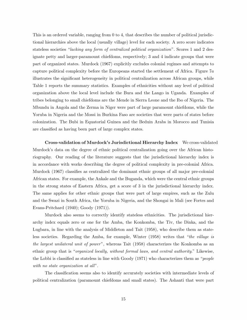
This is an ordered variable, ranging from 0 to 4, that describes the number of political jurisdic-

tional hierarchies above the local (usually village) level for each society. A zero score indicates

stateless societies “lacking any form of centralized political organization”. Scores 1 and 2 des-

ignate petty and larger-paramount chiefdoms, respectively; 3 and 4 indicate groups that were

part of organized states. Murdock (1967) explicitly excludes colonial regimes and attempts to

capture political complexity before the Europeans started the settlement of Africa. Figure 7

illustrates the significant heterogeneity in political centralization across African groups, while

Table 1 reports the summary statistics. Examples of ethnicities without any level of political

organization above the local level include the Bura and the Lango in Uganda. Examples of

tribes belonging to small chiefdoms are the Mende in Sierra Leone and the Ibo of Nigeria. The

Mbundu in Angola and the Zerma in Niger were part of large paramount chiefdoms, while the

Yoruba in Nigeria and the Mossi in Burkina Faso are societies that were parts of states before

colonization. The Bubi in Equatorial Guinea and the Beduin Arabs in Morocco and Tunisia

are classified as having been part of large complex states.

Cross-validation of Murdock’s Jurisdictional Hierarchy Index We cross-validated

Murdock’s data on the degree of ethnic political centralization going over the African histo-

riography. Our reading of the literature suggests that the jurisdictional hierarchy index is

in accordance with works describing the degree of political complexity in pre-colonial Africa.

Murdock (1967) classifies as centralized the dominant ethnic groups of all major pre-colonial

African states. For example, the Ankale and the Buganda, which were the central ethnic groups

in the strong states of Eastern Africa, get a score of 3 in the jurisdictional hierarchy index.

The same applies for other ethnic groups that were part of large empires, such as the Zulu

and the Swazi in South Africa, the Yoruba in Nigeria, and the Shongai in Mali (see Fortes and

Evans-Pritchard (1940); Goody (1971)).

Murdock also seems to correctly identify stateless ethnicities. The jurisdictional hier-

archy index equals zero or one for the Amba, the Konkomba, the Tiv, the Dinka, and the

Lugbara, in line with the analysis of Middleton and Tait (1958), who describe them as state-

less societies. Regarding the Amba, for example, Winter (1958) writes that “the village is

the largest unilateral unit of power”, whereas Tait (1958) characterizes the Konkomba as an

ethnic group that is “organized locally, without formal laws, and central authority.” Likewise,

the Lobbi is classified as stateless in line with Goody (1971) who characterizes them as “people

with no state organization at all”.

The classification seems also to identify accurately societies with intermediate levels of

political centralization (paramount chiefdoms and small states). The Ashanti that were part

15

of a loose confederation get a score of 2; likewise, the Nupe in Northern Nigeria, the Bemba in

Zambia, and the Ngwato in Botswana which were also part of small states get a score of 2 (see

Fortes and Evans-Pritchard (1940)).

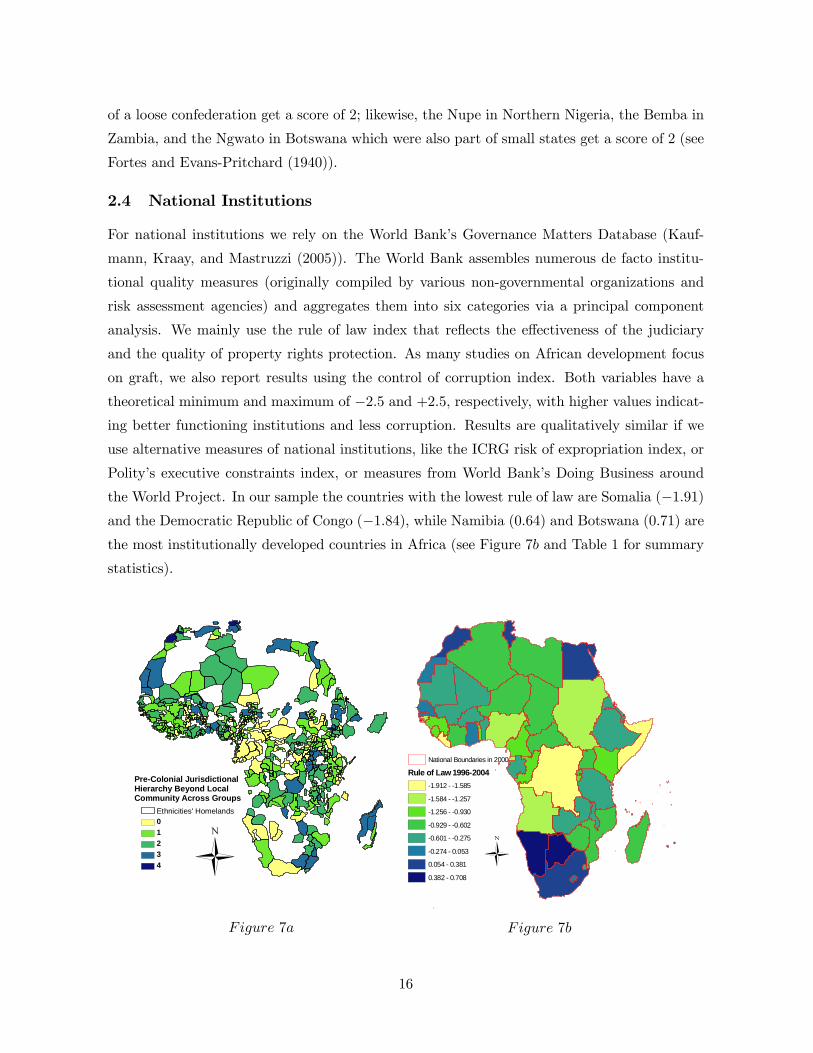
2.4 National Institutions

For national institutions we rely on the World Bank’s Governance Matters Database (Kauf-

mann, Kraay, and Mastruzzi (2005)). The World Bank assembles numerous de facto institu-

tional quality measures (originally compiled by various non-governmental organizations and

risk assessment agencies) and aggregates them into six categories via a principal component

analysis. We mainly use the rule of law index that reflects the effectiveness of the judiciary

and the quality of property rights protection. As many studies on African development focus

on graft, we also report results using the control of corruption index. Both variables have a

theoretical minimum and maximum of −25 and +25, respectively, with higher values indicat-ing better functioning institutions and less corruption. Results are qualitatively similar if we

use alternative measures of national institutions, like the ICRG risk of expropriation index, or

Polity’s executive constraints index, or measures from World Bank’s Doing Business around

the World Project. In our sample the countries with the lowest rule of law are Somalia (−191)and the Democratic Republic of Congo (−184), while Namibia (064) and Botswana (071) arethe most institutionally developed countries in Africa (see Figure 7 and Table 1 for summary

statistics).

Ü

Pre-Colonial Jurisdictional Hierarchy Beyond Local Community Across Groups

Ethnicities' Homelands0

1

2

3

4

7

Ü

National Boundaries in 2000

Rule of Law 1996-2004

-1.912 - -1.585

-1.584 - -1.257

-1.256 - -0.930

-0.929 - -0.602

-0.601 - -0.275

-0.274 - 0.053

0.054 - 0.381

0.382 - 0.708

7

16

2.5 General Empirical Framework

Our analysis on the relationship between contemporary national and pre-colonial ethnic insti-

tutions and regional development is based on variants of the following specification:

= 0 + + + 0Φ+ + [ + ] + (1)

The dependent variable, , is the level of economic activity in the historical homeland

of ethnic group in country , as proxied by light density at night. denotes institutional

quality of country , as reflected in the rule of law and the control for corruption measures. For

ethnicities that fall into more than one country, each area of the partitioned group is assigned

to the corresponding country . For example, regional light density in the part of the Ewe in

Ghana is matched to the institutional quality of Ghana, while the adjacent region of the Ewe

in Togo is assigned the value of Togo. denotes local ethnic institutions as reflected

in the degree of jurisdictional hierarchy beyond the local level.

Since the correlation between luminosity and proxies of development strengthens when

we condition on urbanization in many specifications we control for log population density

() though population density is likely endogenous to national/ethnic institutional devel-

opment. Moreover, when we control for population density the regression estimates capture

the relationship between institutions and economic development per capita.

A potential merit of our regional focus is that we can account properly for local geography

and other factors (captured in vector ). This is non-trivial as there is a fierce debate in

the literature on the institutional origins of development on whether the strong correlation

between institutional and economic development is driven by geographical features and the

disease environment (e.g. Gallup, Sachs, and Mellinger (1999), Easterly and Levine (2003)).

In many specifications we include a rich set of geographic controls, reflecting land endowments

(elevation, area under water), ecological features (malaria stability index, land suitability for

agriculture), and natural resources (diamond mines and petroleum fields).

There are several studies that suggest the inclusion of these variables. First, Nunn and

Puga (2011) show that elevation and terrain ruggedness have affected African development both

via goods and slave trades. Second, the inclusion of surface under water accounts for blooming

in the light image data and for the potential positive effect of water streams on development

via trade. Third, controlling for malaria prevalence is important as Gallup and Sachs (2001)

and subsequent studies have shown a large negative effect of malaria on development. Fourth,

there is a vast literature linking natural resources like oil and diamonds to development and

civil conflict (e.g. Ross (2006)). Fifth, Michalopoulos (2011) shows that differences in land

suitability and elevation across regions lead to the formation of ethnic groups, whereas Fenske

17

(2009) and Ashraf and Galor (2011) show that land quality is strongly correlated with pre-

colonial population densities. We also control for the distance of the centroid of each ethnic

group in country from the capital city, the national border, and the coast. The coefficient

on distance from the capital may reflect the impact of colonization and the limited penetration

of national institutions due to the poor infrastructure (we formally explore this possibility

below). Distance to the border captures the potentially lower level of development in border

areas. Distance to the sea coast captures the effect of trade, but to some extent also the

penetration of colonization. This is because during the colonial era (and the slave trades)

Europeans mainly settled in coastal areas.

In our analysis on the impact of national institutions in Section 3 we include ethnicity

fixed effects () to effectively control for cultural and unobserved geographical features of

ethnic homelands, whereas in Section 4, where we examine the role of ethnic institutions, we

include country fixed effects () to account for differences in national policies and institutions,

as well as other countrywide factors.

2.6 Technical Remarks

Estimation The distribution of luminosity is not normal, as (i) a significant fraction

(around 30%) of the observations takes on the value of zero9 and (ii) we have a few extreme

observations in the right tail of the distribution (see Appendix Figure 1). While the mean

of satellite light density is 0364 the median is more than twenty times smaller, 0017. This

occurs because there are a few ethnic areas where light density is extremely high. For example,

we have 13 observations (1%) where light density exceeds 64 and 26 observations (2%) where

light density exceeds 467.

To account for both issues in many specifications we use as the dependent variable the log

of light density adding a small number (( ≡ ln(001+), see Appendix Figure

1).10 This transformation assures that we use all observations and that we minimize the prob-

lem of outliers. We also estimate specifications ignoring unlit areas ( ≡ ln()),

as in this case the dependent variable is normally distributed (see Appendix Figure 1). More-

over, looking at the "intensive margin" also guarantees that we investigate the role of (national

and ethnic) institutions in explaining variation in economic performance across densely popu-

lated regions displaying non-trivial economic activity. Non-lit areas have a median population

density of 882 people per square kilometer whereas regions with positive light density have a

9A zero level of light density occurs either because the area is extremely sparsely populated without any

electricity or because the satellite sensors cannot capture dimly lit areas.10 In the previous draft of the paper we added one to the luminosity data before taking the logarithm finding

similar results.

18

median of 2763.11 Moreover, in our RD analysis where we use pixels of 0125 0125 decimal

degrees (approximately 1212 kilometers) as the unit of analysis we focus on the "extensive

margin" of luminosity using as the dependent variable a dummy that takes on the value one

when the pixel is lit.

Inference In all specifications we employ the approach of Cameron, Gelbach, and

Miller (2006) and cluster standard errors along two dimensions. Specifically, when the unit

of analysis is an ethnic homeland we cluster at the country and at the ethnic-family level.

Murdock assigns the 834 groups into 96 ethnolinguistic clusters/families. When the unit of

analysis is a pixel within an ethnic homeland we cluster at the country and at the ethnicity

level. This double-clustering accounts for two main concerns related to non-adjusted standard

errors. First, within each country we have several ethnicities where the country-level rule of law

and the control-of-corruption measures take the same value and thus clustering at the country-

level is required (Moulton (1986)). Likewise, partitioned ethnicities appear more than one time

in our sample and thus clustering at the ethnic family accounts for unobserved features within

each ethnolinguistic family. As we report specifications using the ethnicity-level indicators

that exhibit within-ethnic-family correlation, it is appropriate to also cluster standard errors

at the ethnic-family level. Second, the multi-way clustering method accounts for arbitrary

residual correlation within both dimensions and thus accounts for spatial correlation (Cameron,

Gelbach, and Miller (2006) explicitly cite spatial correlation as an application of the multi-

clustering approach). We also estimated standard errors accounting for spatial correlation of an

unknown form using Conley’s (1999) method. The two approaches yield similar standard errors;

and if anything the two-way clustering produces somewhat larger standard errors yielding more

conservative inference. Moreover, as in many specifications we include country or ethnicity fixed

effects this soaks up further the spatial correlation at each dimension.

2.7 Preliminary Evidence

Table 1 reports summary statistics for the variables employed in the empirical analysis. Table 2

reports cross-sectional LS specifications that associate regional development with contemporary

national and pre-colonial ethnic institutions. Below the estimates we report both double-

clustered (in parentheses) and Conley’s (in brackets) standard errors.12 Column (1) shows

11The results are similar if we ignore the top 1%, 2% or 5% of the luminosity data. Moreover, in the previous

version of the paper we reported Poisson ML specifications finding analogous results. We also estimated Tobit

specifications that account for censoring in the dependent variable and also performed least absolute deviation

(median) regressions using all data to account for outliers. These alternative estimation techniques deliver quite

similar results.12Conley’s correction method requires a cut-off distance beyond which the spatial correlation is assumed to

be zero; we experimented with various cutoff values between 100 and 3000 choosing the cutoff of 2000

19

that there is a positive and significant correlation between the rule of law index and regional

development. In column (2) we add population density, whereas in column (3) we control

for distance to the capital city, distance to the border, and distance to the coast ("location

controls"). While all distance terms enter with significant coefficients, the estimate on rule of

law retains its economic and statistical significance. In column (4) we control for population

density, location, and a rich set of geographic controls. Conditioning on geography reduces

the magnitude of the coefficient; yet the estimate retains significance at conventional levels.13

Overall, these correlations echo the findings of cross-country works; although the association

between institutional quality and development weakens when one accounts for geography, it

remains highly significant.

In columns (5) to (8) we associate regional development with ethnic pre-colonial political

institutions. Column (5) reports the unconditional estimate. The coefficient on jurisdictional

hierarchy index is positive and significant at the 99% confidence level. Controlling for popula-

tion density, location, and the rich set of geographic controls (in columns (6)-(8)) reduces the

size of the coefficient, which nevertheless remains at least two standard deviations above zero

in all permutations.

In columns (9)-(12) we regress regional light density on both national and ethnic insti-

tutions. Given the positive correlation (016) between rule of law and jurisdictional hierarchy,

it is useful to investigate the stability of the previous results. Column (9) introduces both the

rule of law index and the jurisdictional hierarchy measure. The unconditional estimate of rule

of law in the sample of 680 ethnicity-country observations is 014 (specification not shown).

Once we control for the degree of jurisdictional hierarchy the estimate on rule of law retains

its significance although it falls by 15%. Likewise, the coefficient on jurisdictional hierarchy

is positive and highly significant, though its magnitude is somewhat smaller compared to the

analogous specification in (5).14 A similar pattern obtains when we control for location (dis-

tance to the border, the sea coast, and the capital city), population density, and the set of

geographic-ecological controls (in (10)-(12)).

The coefficient in column (12) implies that a one point increase in the rule of law index

(roughly 2 standard deviations), which corresponds to moving approximately from the institu-

which delivers the largest in magnitude standard errors.13Land suitability for agriculture, which reflects climatic (temperature and precipitation) and soil conditions,

enters most models with a positive and significant estimate. The malaria stability index enters in all specifica-

tions with a statistically negative estimate. The coefficient on land area under water is positive and in many

specifications statistically significant. Elevation enters with a negative estimate which is significant in some

models. The petroleum dummy enters always with a positive and significant coefficient. The diamond dummy

enters in most specifications with a negative coefficient.14Compared to the specifications in columns (5)-(8), we lose three observations when we include the rule of

law index, because we lack data on Western Sahara (the results are almost identical if we assign the rule of law

index of Morocco to the Western-Saharan ethnic regions).

20

tional quality level of Angola to that of Gabon, is associated with a 070 log points increase in

regional luminosity (approximately 05 standard deviation). This effect is similar in magnitude

to cross-country studies associating log per capita GDP with national institutions (for example

Acemoglu, Johnson, and Robinson (2001) report "standardized" beta coefficients in the range

of 03 − 06). Turning now to the magnitude of pre-colonial institutions, the most conserva-tive LS estimate (017) implies that regional development increases by approximately 50% as

one moves from areas where stateless societies reside to regions with ethnic groups featuring

centralized pre-colonial institutions (i.e. have a jurisdictional hierarchy index equal to 3).

The preliminary results in Table 2 are informative about the broad data patterns. How-

ever, these estimates do not identify the one-way effect of neither contemporary national in-

stitutions nor ethnic historical institutional traits on regional development. This is the task of

the next two sections.

3 National Institutions and Regional Development

Identifying the causal impact of contemporary institutions on regional development is a de-

manding task, because, among other challenges, there are rarely otherwise identical cultures

exposed to different institutional settings. The arbitrary border design in Africa offers an ideal

setting to isolate the effect of nationwide institutions from ethnic-specific characteristics.

There is significant variation in both national institutional quality and luminosity across

African borders. Sharp border discontinuities in rule of law appear in several parts of Africa.

For example, in the Botswana and Zimbabwe border (where the Hiechware, the Subia, and the

Tlokwa are partitioned); across the Namibia and Angola border (where the Ambo are split);

between Kenya and Somalia (where the Bararetta group resides); or between Gabon and Congo

(where the Duma live). Likewise, there are changes in luminosity across the border within the

historical homeland of the same partitioned ethnic group (Figure 8). On the one hand, in

spite of notable differences in national institutions across adjacent countries, in around 30% of

the sample there are virtually no differences in light density across the border within ethnic

groups. On the other hand, in about 40% of the partitions there are more than one log point

differences in luminosity. For example, large jumps in luminosity appear in the Egypt-Sudan

border (where the Ababda and the Barabra groups are partitioned), in the border between

Ghana and the Ivory Coast (where the Assini reside), and between Benin and Togo (where the

Popo are split). To the extent that national institutions affect regional development, one should

expect to find that the part of the ethnic group that belongs to the high institutional quality

country would outperform economically the adjacent region of the same historical homeland

that falls into the country with the relatively worse national institutions.

21

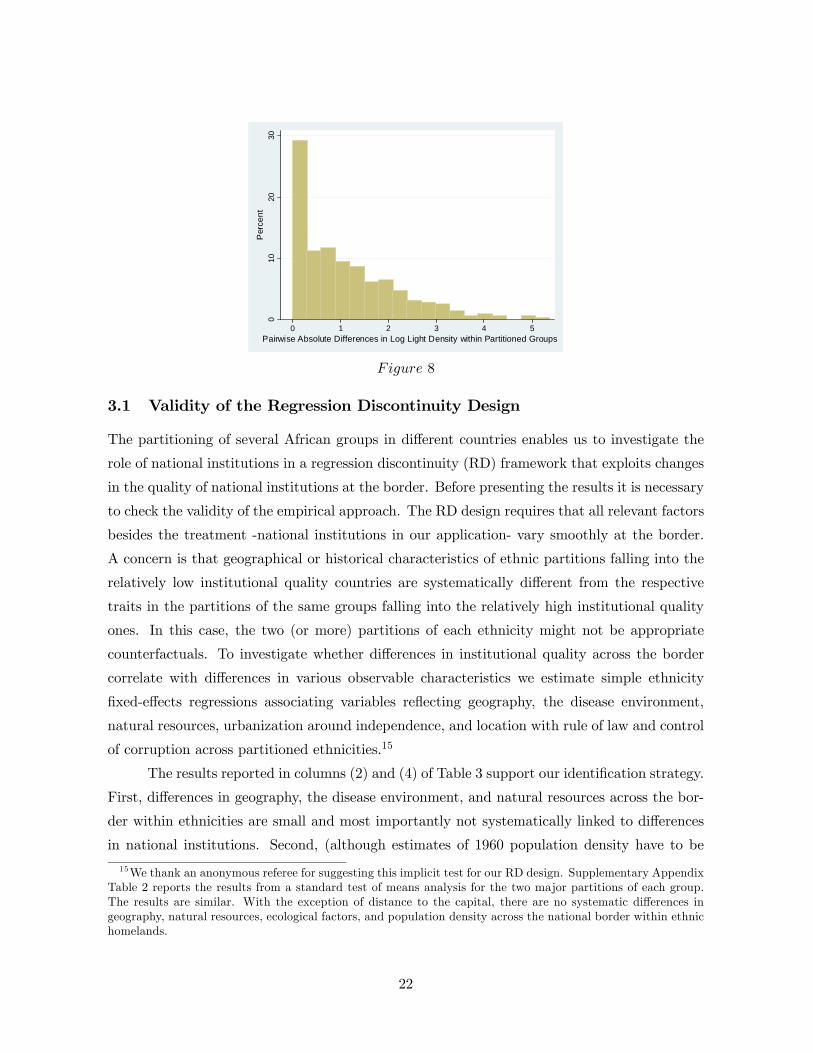
010

2030

Per

cen

t

0 1 2 3 4 5Pairwise Absolute Differences in Log Light Density within Partitioned Groups

8

3.1 Validity of the Regression Discontinuity Design

The partitioning of several African groups in different countries enables us to investigate the

role of national institutions in a regression discontinuity (RD) framework that exploits changes

in the quality of national institutions at the border. Before presenting the results it is necessary

to check the validity of the empirical approach. The RD design requires that all relevant factors

besides the treatment -national institutions in our application- vary smoothly at the border.

A concern is that geographical or historical characteristics of ethnic partitions falling into the

relatively low institutional quality countries are systematically different from the respective

traits in the partitions of the same groups falling into the relatively high institutional quality

ones. In this case, the two (or more) partitions of each ethnicity might not be appropriate

counterfactuals. To investigate whether differences in institutional quality across the border

correlate with differences in various observable characteristics we estimate simple ethnicity

fixed-effects regressions associating variables reflecting geography, the disease environment,

natural resources, urbanization around independence, and location with rule of law and control

of corruption across partitioned ethnicities.15

The results reported in columns (2) and (4) of Table 3 support our identification strategy.

First, differences in geography, the disease environment, and natural resources across the bor-

der within ethnicities are small and most importantly not systematically linked to differences

in national institutions. Second, (although estimates of 1960 population density have to be

15We thank an anonymous referee for suggesting this implicit test for our RD design. Supplementary Appendix

Table 2 reports the results from a standard test of means analysis for the two major partitions of each group.

The results are similar. With the exception of distance to the capital, there are no systematic differences in

geography, natural resources, ecological factors, and population density across the national border within ethnic

homelands.

22

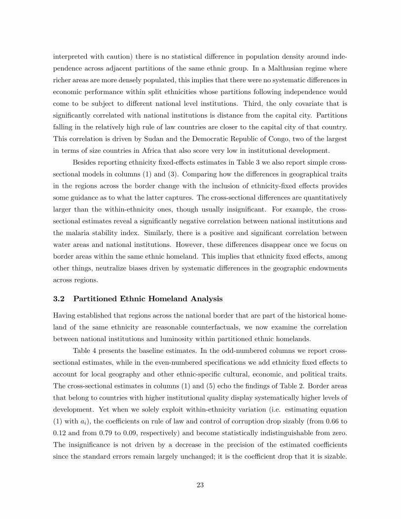
interpreted with caution) there is no statistical difference in population density around inde-

pendence across adjacent partitions of the same ethnic group. In a Malthusian regime where

richer areas are more densely populated, this implies that there were no systematic differences in

economic performance within split ethnicities whose partitions following independence would

come to be subject to different national level institutions. Third, the only covariate that is

significantly correlated with national institutions is distance from the capital city. Partitions

falling in the relatively high rule of law countries are closer to the capital city of that country.

This correlation is driven by Sudan and the Democratic Republic of Congo, two of the largest

in terms of size countries in Africa that also score very low in institutional development.

Besides reporting ethnicity fixed-effects estimates in Table 3 we also report simple cross-

sectional models in columns (1) and (3). Comparing how the differences in geographical traits

in the regions across the border change with the inclusion of ethnicity-fixed effects provides

some guidance as to what the latter captures. The cross-sectional differences are quantitatively

larger than the within-ethnicity ones, though usually insignificant. For example, the cross-

sectional estimates reveal a significantly negative correlation between national institutions and

the malaria stability index. Similarly, there is a positive and significant correlation between

water areas and national institutions. However, these differences disappear once we focus on

border areas within the same ethnic homeland. This implies that ethnicity fixed effects, among

other things, neutralize biases driven by systematic differences in the geographic endowments

across regions.

3.2 Partitioned Ethnic Homeland Analysis

Having established that regions across the national border that are part of the historical home-

land of the same ethnicity are reasonable counterfactuals, we now examine the correlation

between national institutions and luminosity within partitioned ethnic homelands.

Table 4 presents the baseline estimates. In the odd-numbered columns we report cross-

sectional estimates, while in the even-numbered specifications we add ethnicity fixed effects to

account for local geography and other ethnic-specific cultural, economic, and political traits.

The cross-sectional estimates in columns (1) and (5) echo the findings of Table 2. Border areas

that belong to countries with higher institutional quality display systematically higher levels of

development. Yet when we solely exploit within-ethnicity variation (i.e. estimating equation

(1) with ), the coefficients on rule of law and control of corruption drop sizably (from 066 to

012 and from 079 to 009, respectively) and become statistically indistinguishable from zero.

The insignificance is not driven by a decrease in the precision of the estimated coefficients

since the standard errors remain largely unchanged; it is the coefficient drop that it is sizable.

23

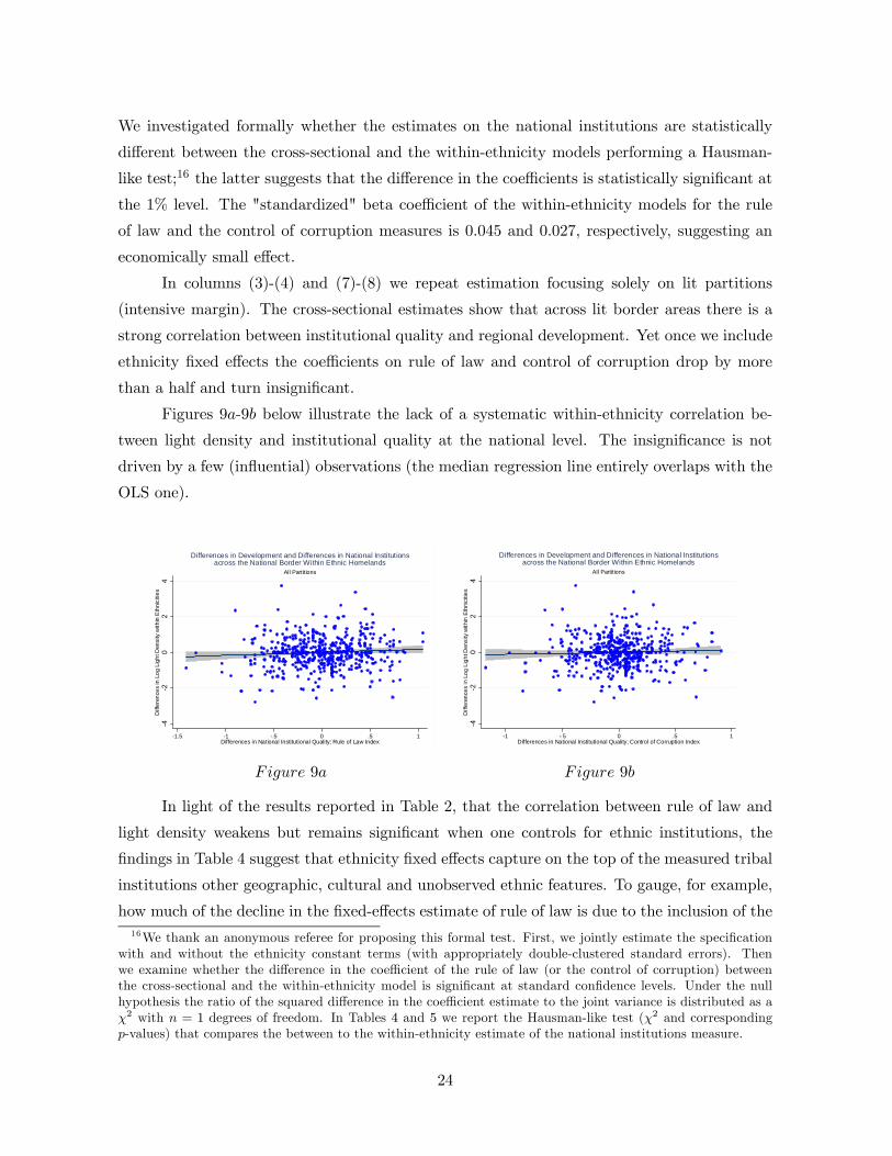
We investigated formally whether the estimates on the national institutions are statistically

different between the cross-sectional and the within-ethnicity models performing a Hausman-

like test;16 the latter suggests that the difference in the coefficients is statistically significant at

the 1% level. The "standardized" beta coefficient of the within-ethnicity models for the rule

of law and the control of corruption measures is 0045 and 0027, respectively, suggesting an

economically small effect.

In columns (3)-(4) and (7)-(8) we repeat estimation focusing solely on lit partitions

(intensive margin). The cross-sectional estimates show that across lit border areas there is a

strong correlation between institutional quality and regional development. Yet once we include

ethnicity fixed effects the coefficients on rule of law and control of corruption drop by more

than a half and turn insignificant.

Figures 9-9 below illustrate the lack of a systematic within-ethnicity correlation be-

tween light density and institutional quality at the national level. The insignificance is not

driven by a few (influential) observations (the median regression line entirely overlaps with the

OLS one).

-4-2

02

4D

iffe

ren

ces

in L

og

Lig

ht D

ensi

ty w

ithin

Eth

nic

itie

s

-1.5 -1 -.5 0 .5 1Differences in National Institutional Quality; Rule of Law Index

All Partitions

Differences in Development and Differences in National Institutionsacross the National Border Within Ethnic Homelands

-4-2

02

4D

iffe

ren

ces

in L

og

Lig

ht D

ensi

ty w

ithin

Eth

nic

itie

s

-1 -.5 0 .5 1Differences in National Institutional Quality; Control of Corruption Index

All Partitions

Differences in Development and Differences in National Institutionsacross the National Border Within Ethnic Homelands

9 9

In light of the results reported in Table 2, that the correlation between rule of law and

light density weakens but remains significant when one controls for ethnic institutions, the

findings in Table 4 suggest that ethnicity fixed effects capture on the top of the measured tribal

institutions other geographic, cultural and unobserved ethnic features. To gauge, for example,

how much of the decline in the fixed-effects estimate of rule of law is due to the inclusion of the

16We thank an anonymous referee for proposing this formal test. First, we jointly estimate the specification

with and without the ethnicity constant terms (with appropriately double-clustered standard errors). Then

we examine whether the difference in the coefficient of the rule of law (or the control of corruption) between

the cross-sectional and the within-ethnicity model is significant at standard confidence levels. Under the null

hypothesis the ratio of the squared difference in the coefficient estimate to the joint variance is distributed as a

2 with = 1 degrees of freedom. In Tables 4 and 5 we report the Hausman-like test (2 and corresponding

-values) that compares the between to the within-ethnicity estimate of the national institutions measure.

24

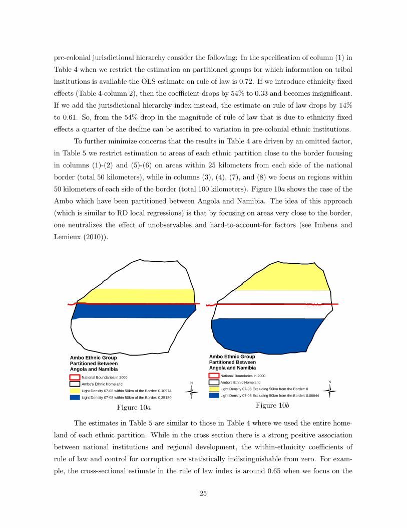
pre-colonial jurisdictional hierarchy consider the following: In the specification of column (1) in

Table 4 when we restrict the estimation on partitioned groups for which information on tribal

institutions is available the OLS estimate on rule of law is 072. If we introduce ethnicity fixed

effects (Table 4-column 2), then the coefficient drops by 54% to 033 and becomes insignificant.

If we add the jurisdictional hierarchy index instead, the estimate on rule of law drops by 14%

to 061. So, from the 54% drop in the magnitude of rule of law that is due to ethnicity fixed

effects a quarter of the decline can be ascribed to variation in pre-colonial ethnic institutions.

To further minimize concerns that the results in Table 4 are driven by an omitted factor,

in Table 5 we restrict estimation to areas of each ethnic partition close to the border focusing

in columns (1)-(2) and (5)-(6) on areas within 25 kilometers from each side of the national

border (total 50 kilometers), while in columns (3), (4), (7), and (8) we focus on regions within

50 kilometers of each side of the border (total 100 kilometers). Figure 10 shows the case of the

Ambo which have been partitioned between Angola and Namibia. The idea of this approach

(which is similar to RD local regressions) is that by focusing on areas very close to the border,

one neutralizes the effect of unobservables and hard-to-account-for factors (see Imbens and

Lemieux (2010)).

Ü

Ambo Ethnic GroupPartitioned Between Angola and Namibia

National Boundaries in 2000

Ambo's Ethnic Homeland

Light Density 07-08 within 50km of the Border: 0.10974

Light Density 07-08 within 50km of the Border: 0.35180

Figure 10

Ambo Ethnic GroupPartitioned Between Angola and Namibia

National Boundaries in 2000

Ambo's Ethnic Homeland

Light Density 07-08 Excluding 50km from the Border: 0

Light Density 07-08 Excluding 50km from the Border: 0.08644 ÜFigure 10

The estimates in Table 5 are similar to those in Table 4 where we used the entire home-

land of each ethnic partition. While in the cross section there is a strong positive association

between national institutions and regional development, the within-ethnicity coefficients of

rule of law and control for corruption are statistically indistinguishable from zero. For exam-

ple, the cross-sectional estimate in the rule of law index is around 065 when we focus on the

25

areas within 25 and within 50 from the national borders. Its magnitude drops by more

than two thirds once we add ethnicity fixed effects and becomes insignificant casting doubt

on the causal interpretation of the simple cross-sectional association between national insti-

tutional quality and regional development. The insignificance is not driven by an increase in

the standard errors. In all permutations two-standard-error bands in the within-ethnicity esti-

mates reported in the even-numbered columns exclude the analogous cross-sectional ones in the

odd-numbered columns. Likewise, the Hausman-type test suggests that the difference in the

coefficient between the cross-sectional and the within-ethnicity model is statistically significant

at standard confidence levels.

3.2.1 Further Evidence and Sensitivity Analysis

In the Supplementary Appendix Tables 3− 7 we report an array of sensitivity checks. Amongothers, we show that the uncovered pattern is robust to different econometric specifications,

alternative transformations of the dependent variable, different mapping of the ethnic home-

lands, and more. Below, we investigate in detail how cross-border migration and a group’s

distance from the capital city may affect our findings.

Migration Anecdotal evidence suggests that national boundaries across Africa are poorly

enforced due to the lack of border patrolling, poor demarcation, and geographic conditions

(desert areas in the North, rainforest in Central Africa). If people migrate to take advantage

of higher incomes in regions with higher levels of institutional quality, mobility across national

boundaries may attenuate income differences across the border. Furthermore, to the extent

that mobility barriers are lower within the same ethnicity compared to moving across different

ethnic homelands, once we focus within the same ethnic group, then the ease of mobility would

further attenuate any differences in regional development caused by changes in the national level

institutions. This scenario predicts that if institutions matter, then as a result of migration

towards the partitions located in the high institutional quality country, population density

should be systematically higher in the latter. Alternatively, it may be the case that population

in the low institutional quality country clusters near the border to migrate daily to the high

institutional quality country to work. Although we have controlled for population density, we

explore in detail the issue of migration with two different approaches.

First, in Table 6 we directly examine the effect of national institutions on population

density using data from the United Nations Environmental Programme.17 There seems to be no

17The UNEP dataset imputes population at the grid level using information on roads,

railroads and navigable rivers as well as information on urban centers (see details at:

http://na.unep.net/siouxfalls/globalpop/africa/part2.html#construct). To further assuage concerns re-

26

systematic association between the quality of national institutions and log population density

in border areas where partitioned ethnicities reside; this applies both to the cross-sectional and

the within-ethnicity estimates, suggesting that the insignificant within-ethnicity relationship

between country-level institutions and regional development is not driven by migration. Note

also that the coefficient is small and even changes sign across permutations. Moreover, to the

extent that population density reflects regional development, the insignificant within-ethnicity

coefficients of rule of law and control of corruption provide additional evidence that national

level institutions are not systematically related to regional economic performance.

Second, we re-estimated our benchmark specifications associating light density with na-

tional institutions across partitioned ethnic homelands excluding areas very close to the border.

Doing so, we account for potential temporary migration flows across the border as well as for

local trade across border regions. By excluding pixels close to the national border we also

account for potential stealing and bleeding (and/or blooming) in the luminosity data. Table

6 reports cross-sectional (in odd-numbered columns) and within-ethnicity specifications (in

even-numbered columns) associating satellite light density and national institutions across par-

titioned ethnic groups excluding the areas close to the border (see Figure 10 for an example).

In columns (1), (2), (5), and (6) we exclude areas within 25 kilometers from each side of the

national border (total 50 kilometers), while in columns (3), (4), (7), and (8) we exclude regions

within 50 kilometers of each side of the border (total 100 kilometers). The results are similar

to the estimates in Tables 4 and 5. While in the cross section there is a strong positive corre-

lation between institutional quality and luminosity, the coefficient drops sizably and becomes

statistically indistinguishable from zero when we add ethnicity fixed effects.

Penetration of National Institutions Europeans’ presence in Africa was (with some ex-

ceptions) limited to the coastline and the capital cities (e.g. Herbst (2000)). Hence, colonial

institutional arrangements, reflected through persistence on today’s institutional quality, would

have limited reach far from the capital cities. Along the same lines, several African scholars

have argued that due to the lack of the necessary infrastructure (roads, transportation system)

and limited state capacity, nationwide institutions have minimal impact far from the capital

cities.18 We explore this hypothesis searching for potential heterogeneous effects of national

lated to measurement error in the population estimates, we also experimented with an alternative measure

from the Gridded Population of the World (http://sedac.ciesin.columbia.edu/gpw/) which does not reallocate

the population, finding again no association between national institutional quality and population density.

Concerns of measurement error in the population density are further toned down because in line with a large

body of work in African historiography we do find a positive association between pre-colonial ethnic institutions

and contemporary population density (see Supplementary Appendix Table 11).18Herbst (2000; pp. 16) notes that "rather systematically, Europeans created capitals that moved power toward

the ocean and away from the interior centers of power that Africans had slowly created". Herbst lists many

27

institutions in ethnic partitions far and close to the capital cities.

Table 7 reports the results. In Panel we focus on two-way split ethnic groups which

have both their partitions close to or far from the respective capital cities (using as a threshold

the median distance to the capital city, 431 ). There are 49 ethnic groups, where both

partitions are relatively close to their capitals (for example, the centroid of Popo’s homeland

in Togo is 51 from Lome, while their homeland in Benin is 72 from Porto-Novo); and

49 groups where both partitions are far from the capital cities (e.g. the Ababda’s homeland

in Sudan is located 630 from Khartoum and their homeland in Egypt is 730 far from

Cairo). The cross-sectional correlation between rule of law and luminosity is twice as strong

for partitions close to the capital vis a vis partitions far from the capital. When we add

ethnicity fixed effects in columns (2) and (4) the coefficients drop by more than half and become

insignificant at conventional levels. Similar pattern obtains when we use all partitioned groups

in Panel . The cross-sectional coefficient on rule of law is positive and significant whereas the

interaction between capital distance and rule of law is negative. This suggests that the positive

cross-sectional correlation between national institutional quality and luminosity decays once we

move further from the capital. For example, combining the coefficients of column (1) of Panel

we get that for ethnic partitions that are further than 1 070 kilometers from the capital

city (this is the case for 10% of the partitions) the cross-sectional correlation is statistically

insignificant. Yet in line with our results so far, once we include ethnicity fixed effects to

account for geographic, institutional and cultural ethnic traits, the coefficient on the rule of law

index becomes statistically indistinguishable from zero. The evidence in Table 7 is consistent

with works from the African historiography that stress the limited penetration of national

institutions far from the capital cities and it complements the literature on optimal country

size (e.g. Alesina and Spolaore (2003)) and state capacity (e.g. Acemoglu (2005); Besley and

Persson (2009, 2010)). Finally, the diminishing effect of national institutions cautions against

generalizing the finding on the non-effect of national institutions for areas around the capital

cities in Africa.19

examples where colonizers decided to ignore local needs and established capital cities outside preexisting polities.

As extreme examples he lists Mauritania and Bechunaland (Botswana) that were ruled during colonization by

capitals outside their nominal territories (Saint-Louis and Mafeking, respectively). Moving the location of the

capital was a key question for African leaders at independence. Yet with a few exceptions (Tanzania, Malawi,

and Nigeria), most countries did not relocate the capital city.19Measurement error in the institutional quality index may also explain the weakening correlation between rule

of law and regional development in areas far from the capital. Since most institutional variables are measured in

the capital cities capturing the rules governing activities of the formal economy, they might not reflect accurately

the institutional features in rural areas (Pande and Udry (2006)).

28

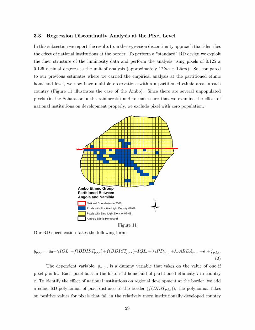
3.3 Regression Discontinuity Analysis at the Pixel Level

In this subsection we report the results from the regression discontinuity approach that identifies

the effect of national institutions at the border. To perform a "standard" RD design we exploit

the finer structure of the luminosity data and perform the analysis using pixels of 0125

0125 decimal degrees as the unit of analysis (approximately 12 12). So, compared

to our previous estimates where we carried the empirical analysis at the partitioned ethnic

homeland level, we now have multiple observations within a partitioned ethnic area in each

country (Figure 11 illustrates the case of the Ambo). Since there are several unpopulated

pixels (in the Sahara or in the rainforests) and to make sure that we examine the effect of

national institutions on development properly, we exclude pixel with zero population.

Ambo Ethnic GroupPartitioned Between Angola and Namibia

National Boundaries in 2000

Pixels with Positive Light Density 07-08

Pixels with Zero Light Density 07-08

Ambo's Ethnic Homeland

ÜFigure 11

Our RD specification takes the following form:

= 0++()+()∗+1+2++

(2)

The dependent variable, , is a dummy variable that takes on the value of one if

pixel is lit. Each pixel falls in the historical homeland of partitioned ethnicity in country

. To identify the effect of national institutions on regional development at the border, we add

a cubic RD-polynomial of pixel-distance to the border (()); the polynomial takes

on positive values for pixels that fall in the relatively more institutionally developed country

29

and negative values for pixels that fall in the relatively less institutionally developed one. We

also add interaction terms between the proxy measures of national institutions () and

the polynomial terms. In many specifications we also control for log pixel population density

() and log pixel area ().

This RD-type design (see Imbens and Lemieux (2008); Lee and Lemieux (2010)) exploits

the discontinuity in the quality of national institutions at the border to identify institutions’

local average treatment effect (LATE).20 The underlying idea is that by comparing pixel-level

economic development across the national border within the same ethnic group, one accounts

for all characteristics that may affect regional development. The results from Table 3 (and

Appendix Table 2) suggest that there are no differences in geography, ecology, and natural

resources within ethnic partitions. This reassures that pixels in the same ethnicity across the

national border are proper counterfactuals.

Previous research has employed variants of the above regression equation using differ-

ent control functions of the running variable (distance to the border) and limiting estimation

close to the discontinuity using different neighborhoods (bandwidths). At the one end, some

researchers use all observations, both far and close to the discontinuity, as this approach max-

imizes the sample and is more efficient (e.g. Lee, Moretti, and Butler (2004)). On the other

end, others estimate local linear regressions limiting their analysis to an area close to the dis-

continuity (e.g. Angrist and Lavy (2001)). Table 8 reports the regression discontinuity results

with both RD approaches proxying national institutional quality with the rule of law index (in

(1)-(4)) and the control for corruption index (in (5)-(8)). Table 1-Panel reports the summary

statistics of light density in this sample.

Cross-Sectional and Ethnicity Fixed-Effects Specifications Before presenting

the RD results, we report in Table 8-Panel A simple LS estimates across pixels. The cross-

sectional coefficients on the rule of law and the control for corruption index in columns (1) and

(5) are positive and highly significant. Yet once we include ethnicity fixed effects (in (2) and (6))

the coefficients on the measures of national institutions become statistically indistinguishable

from zero. The insignificance is not driven by a decrease in the precision of the estimated

coefficients since the standard errors also decline substantially. It is the coefficient that drops

considerably, from 011 to 0017 in the case of rule of law and from 0135 to 0017, in the

20Note that in contrast to most RD applications we do not have a discrete "treatment" group since the national

institutions variable is continuous. We also estimated specifications using as a dependent variable an indicator

that take on the value 1 in the country with the relatively higher measure of institutional development. The

results (not reported for brevity) are similar.

30

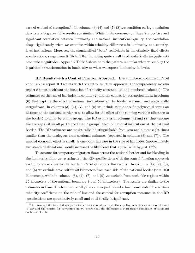
case of control of corruption.21 In columns (3)-(4) and (7)-(8) we condition on log population

density and log area. The results are similar. While in the cross-section there is a positive and

significant correlation between luminosity and national institutional quality, the correlation

drops significantly when we examine within-ethnicity differences in luminosity and country-

level institutions. Moreover, the standardized "beta" coefficients in the ethnicity fixed-effects

specifications, range from 0025 to 0046, implying quite small (and statistically insignificant)

economic magnitudes. Appendix Table 8 shows that the pattern is similar when we employ the

logarithmic transformation in luminosity or when we express luminosity in levels.

RD Results with a Control Function Approach Even-numbered columns in Panel

of Table 8 report RD results with the control function approach. For comparability we also

report estimates without the inclusion of ethnicity constants (in odd-numbered columns). The

estimates on the rule of law index in column (2) and the control for corruption index in column

(6) that capture the effect of national institutions at the border are small and statistically

insignificant. In columns (3), (4), (7), and (8) we include ethnic-specific polynomial terms on

distance to the national border so as to allow for the effect of the running variable (distance to

the border) to differ by ethnic group. The RD estimates in columns (4) and (8) thus capture

the average (within all partitioned ethnic groups) effect of national institutions at the national

border. The RD estimates are statistically indistinguishable from zero and almost eight times

smaller than the analogous cross-sectional estimates (reported in columns (3) and (7)). The

implied economic effect is small. A one-point increase in the rule of law index (approximately

two standard deviations) would increase the likelihood that a pixel is lit by just 17%.

To account for temporary migration flows across the national border and for bleeding in

the luminosity data, we re-estimated the RD specifications with the control function approach

excluding areas close to the border. Panel reports the results. In columns (1), (2), (5),

and (6) we exclude areas within 50 kilometers from each side of the national border (total 100

kilometers), while in columns (3), (4), (7), and (8) we exclude from each side regions within

25 kilometers of the national boundary (total 50 kilometers). The results are similar to the

estimates in Panel where we use all pixels across partitioned ethnic homelands. The within-

ethnicity coefficients on the rule of law and the control for corruption measures in the RD

specifications are quantitatively small and statistically insignificant.

21A Hausman-like test that compares the cross-sectional and the ethnicity fixed-effects estimates of the rule

of law and the control for corruption index, shows that the difference is statistically significant at standard

confidence levels.

31

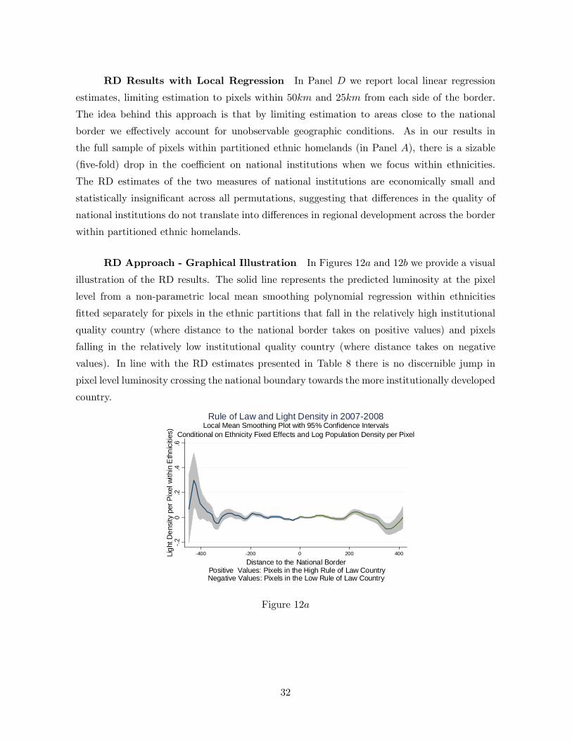
RD Results with Local Regression In Panel we report local linear regression

estimates, limiting estimation to pixels within 50 and 25 from each side of the border.

The idea behind this approach is that by limiting estimation to areas close to the national

border we effectively account for unobservable geographic conditions. As in our results in

the full sample of pixels within partitioned ethnic homelands (in Panel ), there is a sizable

(five-fold) drop in the coefficient on national institutions when we focus within ethnicities.

The RD estimates of the two measures of national institutions are economically small and

statistically insignificant across all permutations, suggesting that differences in the quality of

national institutions do not translate into differences in regional development across the border

within partitioned ethnic homelands.

RD Approach - Graphical Illustration In Figures 12 and 12 we provide a visual

illustration of the RD results. The solid line represents the predicted luminosity at the pixel

level from a non-parametric local mean smoothing polynomial regression within ethnicities

fitted separately for pixels in the ethnic partitions that fall in the relatively high institutional

quality country (where distance to the national border takes on positive values) and pixels

falling in the relatively low institutional quality country (where distance takes on negative

values). In line with the RD estimates presented in Table 8 there is no discernible jump in

pixel level luminosity crossing the national boundary towards the more institutionally developed

country.

-.2

0.2

.4.6

Lig

ht D

ens

ity p

er P

ixel

with

in E

thn

iciti

es)

-400 -200 0 200 400

Distance to the National Border Positive Values: Pixels in the High Rule of Law CountryNegative Values: Pixels in the Low Rule of Law Country

Local Mean Smoothing Plot with 95% Confidence IntervalsConditional on Ethnicity Fixed Effects and Log Population Density per Pixel

Rule of Law and Light Density in 2007-2008

Figure 12

32

-.2

0.2

.4.6

Ligh

t D

ensi

ty p

er P

ixe

l with

in E

thni

citie

s)

-400 -200 0 200 400

Distance to the National BorderPositive Values: Pixels in the High Control of Corruption CountryNegative Values: Pixels in the Low Control of Corruption Country

Local Mean Smoothing Plot with 95% Confidence IntervalsConditional on Ethnicity Fixed Effects and Log Population Density per Pixel

Control of Corruption and Light Density in 2007-2008

Figure 12

3.4 Results with Afrobarometer Data

We repeated our analysis using data from the 2005 Afrobarometer household surveys on various

measures of public goods provision (and education) as the dependent variable. Doing so the

sample reduces to 32 ethnic groups with at least one enumeration area in each of the partitions

across the countries that the Afrobarometer surveys cover. Nevertheless, it is useful repeating

the analysis in this sample both for cross-validation purposes and because one of the primary

channels associating institutions with development is via the provision of public goods. Our

specification reads:

= 0 + + () + () ∗ + + + (3)

The dependent variable, , reflects average household’s access to an electricity grid,

access to piped water, access to sewage system, and average years of schooling in Afrobarom-

eter’s enumeration area, , that falls in the historical homeland of ethnicity in country .

Since we have multiple households in each enumeration area we take the average. Panel

in Appendix Table 1 reports summary statistics for the dependent variables. Besides report-

ing simple cross-sectional and within-ethnicity results (i.e. including ), we also estimate

regression discontinuity models augmenting the specification with a third-order polynomial on

distance of each enumeration area to the national border, allowing the polynomial terms to

be different in areas falling in the relatively high versus the relatively low institutional quality

country (()); we also include interactions of the cubic polynomial with national

institutions, ; so in these specifications the coefficient on the rule of law or the control

33

for corruption index identifies the local effect of national institutions at the border.

Table 9 reports results associating rule of law (in columns (1)-(4)) or control of corrup-

tion (in columns (5)-(8)) with the household-based proxy measures of development from the

Afrobarometer surveys. We start our analysis replicating our previous findings with luminosity.

Panel reports estimates associating national institutions and luminosity across Afrobarome-

ter’s enumeration areas (luminosity is calculated within a 10 radius from each enumeration

area’s centroid). Column (1) shows that there is a highly significant positive association be-

tween rule of law and luminosity across cities/villages across partitioned ethnic groups. The

correlation weakens considerably and even changes sign when we include ethnicity fixed effects

(in (2)). Augmenting the specification with a global third-order RD polynomial on distance of

each enumeration area to the national border and its interactions with national institutions, so

as to estimate the local effect of rule of law at the border, yields similar (insignificant) results.22

We obtain similar results when we use the control of corruption index. There seems to be no

systematic association between luminosity and national institutions across the border within

partitioned ethnic homelands.

In Panel we use as the dependent variable the mean household access to an electricity

grid within each enumeration area (the average access to electricity across Afrobarometer’s

enumeration areas is 535%; see Appendix Table 1). The cross-sectional estimates show that

household’s access to electrification is greater in countries scoring higher in the two national

institutional quality measures. Yet once we focus within the same ethnic homeland to examine

whether households’ access to an electricity grid is higher in countries with more developed

national institutions, the correlation weakens considerably and in most cases changes sign.

In Panel we associate national institutions with the average household access to piped

water across Afrobarometer’s enumeration areas (the mean is 049). Adding ethnicity fixed

effects to exploit across-the-border variation in villages/towns (enumeration areas) of the same

ethnic group, the positive (and significant) cross-sectional relationship turns insignificant; not

only the coefficient on the rule of law and the control for corruption measures is statistically

insignificant, but the estimate is negative in all permutations.

In Panel we examine whether access to sewage system is systematically associated with

national institutions (on average access to a sewage system is 024) whereas in Panel we use as

the dependent variable average years of schooling across respondents within each enumeration

area (on average household heads have 3 years of formal education). The estimates, albeit less

precisely estimated, echo our previous results. Across all permutations the within-ethnicity

22We cannot estimate local linear regressions with the Afrobarometer data because the sample size of Afro-

barometer enumeration areas drops considerably when limiting attention to areas very close to the national

border.

34

coefficients on rule of law and control for corruption are statistically insignificant.

Summary The estimates in the sub-sample of partitioned ethnic homelands based

on micro-level data reflecting public goods provision and education from the Afrobarometer

surveys lend further support to our benchmark results where we used luminosity to proxy eco-

nomic development. While national institutions correlate positively (and in some specifications

significantly) with access to electricity, access to piped water, access to sewage system, and

schooling across the cities/villages of Afrobarometer surveys, the correlation turns insignificant

and often changes sign when we add ethnicity fixed effects. The analysis, therefore, suggests

that our benchmark estimates using satellite light density are not an artifact of the dependent

variable employed.

4 Pre-colonial Ethnic Institutions and Development

We now turn our focus on the impact of pre-colonial ethnic institutions on contemporary

regional development. In Section 41 we report results at the ethnic homeland level whereas in

Section 42 we perform the analysis at the pixel level.

4.1 Ethnic Homeland Analysis

4.1.1 Benchmark Estimates

The preliminary results in Table 2 reveal a significant association between the complexity

of pre-colonial political structures and regional development. The correlation between pre-

colonial ethnic institutions and regional development retained significance when we controlled

for geography, the disease environment and urbanization. Yet the positive correlation between

local institutions and regional development may be driven by country-level characteristics,

reflecting national policies, the type of colonization, etc. In Table 10 we estimate within-

country specifications associating regional development with pre-colonial ethnic institutions.

Panel reports estimates using all observations, while in Panel we focus on the intensive

margin of luminosity.

Jurisdictional Hierarchy beyond the Local Community Level The coefficient

on the jurisdictional hierarchy index in column (1) is 033 and more than three standard

deviations larger than zero.23 The estimates are only slightly smaller than the analogous

23 In the pre-colonial sample when we add country fixed effects we lose one observation. This is because for

Swaziland we have only one group with information on pre-colonial institutions, the Swazi.

35

unconditional specifications (reported in Table 2 column (5)), suggesting that common-to-all-

ethnicities country-level factors are not driving the positive correlation.24 In column (2) we

augment the specification with distance to the coast, distance to the border, distance from the

capital and the rich set of geographic controls. The coefficient on the jurisdictional hierarchy

beyond the local community level index retains its statistical and economic significance. In

column (3) we control for population density only, while in column (4) we control jointly

for geography, location, and population density. The estimate on the jurisdictional hierarchy

index retains statistical significance, although it falls by almost a half; this is not surprising as

according to the African historiography (see Stevenson (1968), Herbst (2000)) there is a strong

interplay between geography, population density, and political complexity.25 The magnitude

of the coefficient in column (3) of Panel implies that a one-standard-deviation increase in

the jurisdictional hierarchy index (which corresponds to a one-unit increase; see Table 1) is

associated with a 012-standard-deviation increase in regional luminosity. For comparison the

"beta" coefficient on the within-ethnicity estimates on the effect of national institutions on

regional development in Table 4 was around 0025 − 0042. So, the impact of ethnic-specificinstitutions on regional development is more than three times larger than the (insignificant)

effect of national institutions.

Political Centralization In columns (5) and (8) we use an alternative binary indi-

cator of pre-colonial institutions. Following Gennaioli and Rainer (2006, 2007) we construct

a dummy variable of pre-colonial political centralization (statehood) that takes the value of

zero when Murdock’s jurisdictional hierarchy indicates that the tribe lacks a centralized polit-

ical organization or is part of a small chiefdom; the index equals one if Murdock classifies the

ethnicity as being a large chiefdom or part of a state. Experimenting with the re-scaled in-

dex is useful, because the aggregation may account for measurement error in the jurisdictional

hierarchy index.26 Moreover, the binary classification is more in line with the distinction of

African ethnic political systems into strong ones and societies lacking centralized political ad-

24 In line with this, the Hausman-type test that compares the coefficient on the jurisdictional hierarchy index of

the cross-sectional to the within-country model, suggests that we cannot reject the null hypothesis of coefficient

equality.25Note that since population density may be both a cause and an effect of ethnic institutions, the specifications

where we also control for population density (in (3), (4), (7), and (8)) should be carefully interpreted. Following

Angrist and Pishcke’s (2008) recommendation we also used lagged (at independence) population density as a

control. In these models (not reported) the estimates on the ethnic institutions measures are somewhat larger

(and always significant at the 95% confidence level).26To further examine the impact of pre-colonial local institutions, we estimated specifications with four in-

dicator variables that take on the value one when the jurisdictional hierarchy index takes the value 1, 2, 3,

and 4 respectively, with the omitted category being the stateless societies. In line with the results of Table 10

these unrestricted specifications with the four indicator variables show that the higher the degree of pre-colonial

centralization the higher light density is today.

36

ministrative structures (Fortes and Evans-Pritchard (1940)).27 The within-country coefficient

on political centralization is positive and highly significant. The estimate retains significance,

when we control for geography (in (6)), current levels of population density (in (7)) or both

(in (8)). The magnitude of political centralization in column (8) in Panel suggests that

luminosity is 30 percent ((026) − 1 = 030) higher in ethnic homelands where politically

centralized societies reside (e.g. Yoruba in Nigeria), as compared to stateless societies or small

chiefdoms (e.g. the Sokoto or the Tiv in Nigeria).

These results advance the findings of Gennaioli and Rainer (2007), by showing that even

when one accounts for regional geographic endowments and country fixed effects, the correlation

between pre-colonial political centralization and regional development remains strong. The

estimates are supportive of an old conjecture among African scholars that dates at least back

to Fortes and Evans-Pritchard (1940) on the importance of pre-colonial ethnic institutions

in the process of African development. Our results are also in line with the cross-country

evidence of Bockstette, Chanda, and Putterman (2002) on the role of statehood experience on

contemporary development.

4.1.2 Institutions or Other Ethnic Traits?

One concern with the estimates in Table 10 is that some other deeply-rooted ethnic feature, re-

lated to the organization of the economy, social norms, early development, or societal structure,

is driving the positive correlation between luminosity and pre-colonial political centralization.

We thus examined whether political centralization rather than some other ethnic trait corre-

lates with contemporary development utilizing information from Murdock (1967). In Table 11

we report within-country specifications associating log light density with around twenty differ-

ent variables from Murdock’s Ethnographic Atlas (see the Data Appendix for detailed variable

definitions).28 These measures reflect the type of economic activity (dependence on gathering,

hunting, fishing, animal husbandry, milking of domesticated animals, and agriculture), societal

arrangements (polygyny, presence of clans at the village level, slavery), early development (size

and complexity of pre-colonial settlements), and some proxies of local institutional arrange-

ments (namely an indicator for the presence of property rights, elections for local headman,

ethnic class stratification and jurisdictional hierarchy at the local community).

27Fortes and Evans-Pritchard (1940) argue that "the political systems fall into two main categories. One group

consists of those societies which have centralized authority, administrative machinery, and judicial institutions-

in short, a government-and in which cleavages of wealth, privilege, and status correspond to the distribution of

power and authority. This group comprises the Zulu, the Ngwato, the Bemba, the Banyankole, and the Kede. The

other group consists of those societies which lack centralized authority, administrative machinery, and judicial

institutions-in short which lack government-and in which there are no sharp divisions of rank, status, or wealth.

This group comprises the Logoli, the Tallensi, and the Nuer."28We are grateful to an anonymous referee for proposing this test.

37

In Specification (reported in the first two columns) we regress regional light density

on the ethnic-level variables, simply conditioning on country fixed effects and on population

density. Most of the additional variables are statistically insignificant. An indicator that takes

the value 1 for societies where fishing contributes more than 5% in the pre-colonial subsistence

economy enters with a positive coefficient as current economic development is higher in areas

close to the sea and other streams and potentially because of blooming. An agricultural in-

tensity index ranging from 0 to 9 where higher values indicate higher dependence is negative

and significant but the correlation between pre-colonial agricultural intensity and regional de-

velopment is not robust to an alternative index of agricultural intensity. More importantly,

the results in columns (1)-(2) show that ethnic class stratification, a societal trait that has

been linked to property rights protection (e.g. Rudmin (1995)), correlates significantly with

luminosity; this suggests that regional development is higher in areas where stratified (as com-

pared to egalitarian) societies reside. The positive association between class stratification and

regional development, though surprising at first glance, is in line with recent works in Latin

America (e.g. Acemoglu, Bautista, Querubin, and Robinson (2008), Naritomi, Soares, and As-

sunção (2009), Dell (2010)). The main explanation is that in weakly institutionalized societies

inequality may lead to some form of property rights protection, as the elite has the incentive

to establish constraints (see Goldstein and Udry (2008) who show a positive link between po-

litical power inside the local community (class stratification) and land tenure (property rights)

in rural Gambian communities).

In Specification , reported in columns (3)-(5), we add the jurisdictional hierarchy be-

yond the local community index to test whether pre-colonial ethnic political centralization

correlates with current regional development conditional on the other historical ethnic traits.

In all specifications the jurisdictional hierarchy beyond the local community level index enters

with a positive and stable coefficient (around 020), quite similar in magnitude to the (more

efficient) estimates in Table 10. The coefficient is always significant at standard confidence

levels (usually at the 99% level). The most conservative estimate implies that regional de-

velopment, as reflected in luminosity, increases by approximately 45 percent when one moves

from the homeland of a stateless society (e.g. Lango in Uganda) to the historical homeland

of an ethnicity with a hierarchical political structure beyond the local level (e.g. Ganda in

Uganda). The results in Table 11 suggest that the positive within-country association between

the complexity of pre-colonial political institutions and contemporary regional development is

not driven by other deeply-rooted ethnic traits.

38

4.1.3 Contiguous-Ethnic-Homeland Analysis

In spite of employing a rich conditioning set it is conceivable that some unobservable geographic

features are driving the results. To account for this possibility in Table 12 we report results from

a contiguous-homelands analysis where we compare regional development of bordering ethnici-

ties having different degrees of pre-colonial political centralization.29 The rationale behind this

type of adjacent-region analysis is that it will neutralize the effect of hard-to-account-for geo-

graphical/ecological features that vary smoothly across contiguous territories. Our specification

reads:

∆ = 0 + ∆ +∆0Φ+

The dependent variable is the difference in log luminosity between the historical homeland

of ethnicity and the adjacent homeland of ethnicity .30 Our interest is in the coefficient

on the difference in the jurisdictional hierarchy beyond the local community index between

ethnicity and the contiguous ethnic group(s) . We have 258 unique adjacent ethnic pairs

comprising a centralized and a non-centralized ethnicity. When an ethnic group is adjacent to

more than one ethnicities with different pre-colonial centralization we include all such pairs in

the analysis. For example, the Acholi a non-centralized group in Uganda is adjacent to two

centralized groups, the Nyoro in Uganda and the Didinga in Sudan. The median (average)

distance between the centroids of neighboring ethnicities is 179 (215).

Panel reports estimates without conditioning on (differences in) log population den-

sity, while in Panel we control for differences in log population density. The estimates in

(1) show that luminosity is significantly higher in the historical homeland of ethnicities with

more complex pre-colonial political institutions. Controlling in (2) for differences in location,

geography/ecology, and natural resources has no effect on the estimate of interest. In columns

(3) and (4) we repeat the analysis requiring that both contiguous ethnic areas (of groups and

) are in the same country (in this case, for example, we drop the Acholi-Didinga pair because

the homelands of these groups belong to different countries). The results remain intact. Within

countries regional development is significantly higher in areas where tribes with centralized pre-

colonial institutions reside, as compared to their neighboring groups lacking strong pre-colonial

institutions.

29 In some sense this approach extends the pioneering case study of Douglas (1962), who attributed the large

differences in well-being between the Bushong and the Lele to their local institutions. We are thankful to Jim

Robinson for providing us with this reference.30Note that in the adjacent-ethnic-group regressions the unit of analysis are pairs of ethnic homelands for

which there is information on pre-colonial jurisdictional hierarchy. So, all relevant statistics are derived at the

ethnicity level. For example, ∆ = ln(001 + )− ln(001 + ).

39

In columns (5)-(6) and (7)-(8) we restrict our analysis to pairs of contiguous ethnicities

with large differences in jurisdictional hierarchy to account for measurement error in Mur-

dock’s classification of precolonial political centralization; this is also useful to check whether

large differences in pre-colonial institutions translate in significant differences in contemporary

development. In columns (5)-(6) we require a difference of at least two levels in the juris-

dictional hierarchy index, while in (7)-(8) we compare development between adjacent ethnic

groups with the maximum difference in the respective index of pre-colonial institutions (i.e.

∆ = 3−3). There is a strong positive correlation between differences in lumi-nosity and differences in the degree of pre-colonial political institutions. A couple of examples

illustrate the point. In South Africa the average luminosity in the historical homeland of the

Sotho, a highly centralized group, is 068, while luminosity in the neighboring ethnic homeland

of the Xam, a stateless society, is 013. Likewise, in Burkina Faso the average luminosity in the

homeland of the Mossi, the dominant ethnic group of the pre-colonial Mossi empire that gets

a score of 3 in the jurisdictional hierarchy index, is 027, while it is ten times smaller, 0027

in the adjacent ethnic area of the Samo that lack any level of political authority beyond the

local community. Similarly, average luminosity in the homeland of the Ganda, the central eth-

nic group of a strong pre-colonial kingdom in Uganda that had a centralized authority (under

the kabaka/king), is much higher (048) compared to the neighboring territory of the stateless

Lango (0023).

It is important to note that in both Panels of Table 12 the introduction of geographic

and location controls across specifications does not affect the stability of the coefficient on the

differences in political complexity. This pattern assuages (albeit not entirely resolves) concerns

that the positive correlation between pre-colonial ethnic institutions and regional development

is driven by unobserved characteristics related to local endowments and geography.

4.2 Pixel-Level Analysis

As in our analysis on the effect of national institutions on regional development, we estimated

specifications associating luminosity with pre-colonial ethnic institutions using as the unit of

analysis pixels of 0125 0125 decimal degrees. Performing the analysis at the pixel level

allows us to account for the possibility that luminosity at the ethnic homeland level also reflects

inequality. This is the case when average light density is driven by a few extremely lit areas.31

Moreover, utilizing the finer structure of the luminosity data we may also perform a regression

discontinuity analysis across ethnic borders, similar in spirit to our analysis on the effect of

31We thank an anonymous referee for alerting us to this possibility. To further account for this issue we

estimated models excluding ethnic homelands where capital cities fall. The results are similar (see Appendix

Table 10).

40

national institutions at the national border (in Section 33).

4.2.1 Benchmark Estimates

In Table 13 we report LS estimates associating pixel-level luminosity with pre-colonial political

institutions.32 The econometric specification reads:

= 0 + + + 1 + 2 + 0Φ+

The dependent variable, , is economic activity in pixel that belongs to the historical

homeland of ethnicity in country . Panel reports linear probability models where the

dependent variable equals one if the pixel is lit and zero otherwise.33 To illustrate that our

benchmark estimates in Section 41 are not driven by the transformation of the luminosity

data, in Panel we report specifications using as the dependent variable the natural log of

luminosity at the pixel level adding a small number (001).

The coefficient on the jurisdictional hierarchy index in column (1) is positive and highly

significant. The estimate retains significance in column (2) when we control for differences in log

pixel area () and log pixel population density (). In column (3) we introduce

a host of ethnicity-country characteristics, 0. In particular, we condition on distance to

the sea coast, distance to the capital city, distance to the national border, natural resources,

land suitability for agriculture, mean elevation, surface area, land area under water, and a

malaria stability index at the ethnicity-country level. In spite of the inclusion of this rich set of

controls, jurisdictional hierarchy beyond the local community continues to enter with a positive

and highly significant (at the 99% confidence level) coefficient.

The specifications in columns (4)-(6) include country fixed effects. Doing so has little

effect on the coefficient on the pre-colonial ethnic institutions; the estimate is stable (around

0035 − 0045) and highly significant. The coefficient implies that a one-point increase in the0 − 4 scale index capturing the complexity of pre-colonial political structures increases thelikelihood that a pixel is lit by 4%. The standardized "beta" coefficient is around 0125 for

both estimates in Panel and Panel . This is quite similar to the economic effect implied

by the estimates in our analysis at the ethnic homeland level in Section 41. The implied

economic effect of pre-colonial ethnic institutions on regional development at the pixel level is

32As in our previous estimates on the effect of national institutions on development at the pixel level, we focus

on populated areas (i.e. we exclude pixels with zero population). Table 1-Panel reports summary statistics

in this sample.33Probit ML estimates yield similar in magnitude marginal effects (evaluated at the mean of the independent

variables).

41

thus more than three times larger than the implied (statistically insignificant) effect of national

institutions found in Table 8

4.2.2 Contiguous Ethnic Homelands

We also estimated models associating development at the pixel level with pre-colonial ethnic

institutions within pairs of adjacent ethnicities with a different degree of political complexity.

This approach is similar to the framework employed in Section 413 where we used ethnic

homelands (rather than pixels) as the unit of analysis. Our specification reads:

() = 0 + + + 1 + 2 + ()

The dependent variable takes on the value of one if pixel is lit and zero otherwise.

Every pixel falls into the historical homeland of ethnicity that is adjacent to the homeland

of ethnicity (where ethnicities and differ in their degree of pre-colonial centralization,

). All specifications include ethnicity-pair fixed effects, . Therefore, the coeffi-

cient on the jurisdictional hierarchy beyond the local community index, , captures whether

differences in the complexity of pre-colonial ethnic institutions translate into differences in light

density across pixels within pairs of contiguous ethnicities. We perform the analysis within 68

adjacent ethnic pairs (in total 136 ethnicities) with different pre-colonial political institutions.

In case of ethnic homelands having multiple neighbors with different pre-colonial centraliza-

tion we chose the largest in size bordering group (so as to maximize the sample size). So, for

example in the case of the Acholi group that borders the Nyoro and the Didinga, since the

largest group in terms of surface area is the Nyoro, we include in the specification only the

Acholi-Nyoro pair.

Table 14 reports the results. The estimate on the jurisdictional hierarchy index in

columns (1)-(2) is positive and significant at standard confidence levels. Within adjacent ethnic

homelands where groups of different ethnic institutions reside, there is a significantly higher

probability that a pixel is lit if it falls in the historical homeland of the ethnicity that scores

higher in the jurisdictional hierarchy index. In columns (3)-(4) we restrict estimation to groups

that fall in the same country. The coefficient on the jurisdictional hierarchy beyond the lo-

cal community retains its statistical significance and if anything increases in magnitude. The

estimate in column (4) implies that within contiguous ethnic homelands, the probability that

a pixel is lit is approximately 3% higher if it is part of the historical homeland of an ethnic

group with more complex political institutions. In columns (5)-(6) we examine the association

between regional development and ethnic institutions across contiguous ethnic homelands in

the same country with large differences in the jurisdictional hierarchy index (greater than 1

42

unit). In this sample the estimate on the pre-colonial ethnic institutions is positive and highly

significant. For example, in Uganda the Acholi, a society organized in small local chiefdoms,

borders the Nyoro (Bunyoro), a group with complex local institutions that was part of the most

powerful traditional kingdoms in Eastern Africa. As a result 2% of the pixels falling in the

homeland of the Acholi are lit compared to 41% of the pixels in the homeland of the Nyoro.

4.2.3 RD within Contiguous Ethnic Homelands

Table 15 reports estimates, otherwise identical to Table 14, including in the specifications a

third-order RD polynomial on distance of the centroid of each pixel to the ethnic border;

distance takes positive values for pixels in the politically centralized ethnicities and negative

values for pixels in the non-centralized groups.

Performing, however, a standard RD approach across ethnic borders is not as straightfor-

ward as in the case of national borders for several reasons. First, while contemporary national

borders are accurately delineated, there is clearly some error in Murdock’s original map on the

exact location of ethnic boundaries. Second, since Murdock’s map (originally printed in the

end of his book on African ethnicities) is available at a small scale its digitization magnifies

any noise inherent to the initial border drawing. Third, Murdock assigns each area into a sin-

gle dominant ethnic group, while (some) ethnicities (may) overlap; and naturally population

mixing is higher closer to an ethnic boundary. As such the discontinuity, i.e. the point at

which ethnic-specific institutions change, is unlikely to occur exactly at the ethnic border as

delineated in Murdock’s map.

To account for these issues we exclude areas close to the ethnic border. Essentially,

this boils down to assuming that the border is "thick". Then we calculate for each pixel the

distance from the "thick" border. Such an approach allows us to account for population mixing

in the areas along the ethnic boundary and the measurement error in the drawing of the latter.

Excluding areas close to the ethnic border also accounts for bleeding in the luminosity data

and the fact that electricity grids are likely to be crossing adjacent regions within the same

country.

To illustrate that our results are not sensitive to the exact threshold, in Table 15 we

report estimates excluding areas of 50 (Panel ), 75 (Panel ), and 100 (Panel )

from each side of the ethnic border. The estimate on the pre-colonial institutions index in

columns (1) and (2) is positive and significant across all permutations. In columns (3) and (4)

we restrict estimation on neighboring ethnicities that belong to the same country to account for

all nationwide factors that may affect regional development. The coefficient on the jurisdictional

hierarchy index is more than two standard errors larger than zero across all specifications. In

43

columns (5) and (6) we focus on pairs of ethnicities with sharp discontinuities in the strength

of pre-colonial ethnic institutions. The estimates show that regional development, as reflected

in light density at night at the pixel level, is much higher in the homeland of societies with

advanced pre-colonial ethnic institutions. The magnitude of the coefficient in Panel implies

that within pairs of adjacent ethnicities the probability that a pixel is lit is 68% higher if it

falls in the homeland of a group with centralized pre-colonial political institutions.

5 Conclusion

We study the role of institutional quality in shaping contemporary comparative development in

Africa focusing both on formal nationwide structures and informal ethnic-specific arrangements.

We perform our analysis at the regional level utilizing anthropological and historical data on

the spatial distribution and local institutions of African ethnicities at the time of colonization.

To circumvent data unavailability on regional development in Africa we use satellite data on

light density at night to measure economic performance across ethnic homelands. Exploiting

within-ethnicity across-country variation on contemporary country-level institutions as well as

within-country across-ethnicity variation in ethnic pre-colonial institutions, we document new

empirical regularities on the role of institutional structures on African development.

First, we take advantage of the fact that the arbitrarily drawn national boundaries across

the African landscape partitioned groups in different countries, thus subjecting identical cul-

tures to different country-level institutions. Focusing on these groups we show that differences

in economic performance within ethnicities partitioned across different countries cannot be

explained by countrywide differences in institutional quality. We obtain similar results for a

subset of partitioned ethnic homelands for which we have micro-data on household’s access to

public goods from the Afrobarometer Surveys. While this result does not necessarily generalize

to areas far from the national borders, close to the capital cities or other parts of the world,

it casts doubt on the causal interpretation of the cross-country positive correlation between

institutional quality and economic development in Africa.

Second, we explore the significant heterogeneity of historical ethnic institutions and ex-

amine their role on regional development. In line with an influential conjecture among African

scholars, we show that the complexity of ethnic pre-colonial institutions correlates significantly

with contemporary regional development, even when we control for local geography, country-

characteristics, and other ethnic traits. Since we do not have random assignment on ethnic

institutions, this correlation does not necessarily imply causation. Yet the positive correlation

between ethnic political complexity and luminosity is present when we examine the association

within pairs of adjacent ethnic homelands where groups with different pre-colonial institutions

44

reside. Our analysis therefore provides large-scale formal econometric evidence in support of

the African historiography that emphasizes the importance of ethnic institutions and other

historical features in shaping contemporary economic performance suggesting that research on

African development needs to focus at the ethnicity rather than the country level.

On a broader scale, our codification of partitioned ethnic groups and the combination

of high resolution proxies of development (such as satellite light density at night) with his-

torical measures on culture and institutions provide a platform for subsequent research. One

may employ our approach to shed light on the perennial debate regarding the fundamental

determinants (correlates) of comparative economic development across countries; examining,

for example, the effect of human capital, financial development, public policies, and democracy

on economic performance in areas close to the national borders. Moreover, one could investi-

gate how pre-colonial ethnic features interact with contemporary public policies to determine

regional development.

45

6 Data Appendix

6.1 Variables at the ethnicity-country level

Light Density at Night: Light Density is calculated averaging light density observations

across pixels that fall within the unit of analysis. We use the average of the values in 2007

and 2008. In the regressions at the ethnic homeland we use Log (0.01 + Average Luminosity)

or Log (Average Luminosity). In the regressions at the pixel level we use as the dependent

variable a dummy variable that takes on the value of one if the area is lit and zero otherwise.

Source: Available at http://www.ngdc.noaa.gov/dmsp/global_composites_v2.html.

Population Density: Log (0.01 + population density per sq. km. in 2000 or in 1960).

Source: Nelson, Andy, 2004. African Population Database Documentation, UNEP GRID Sioux

Falls. Available at: http://na.unep.net/siouxfalls/datasets/datalist.php

Water Area: Log (1 + total area covered by rivers or lakes in sq. km.). Source:

Constructed using the "Inland water area features" dataset from Global Mapping International,

Colorado Springs, CO, USA. Global Ministry Mapping System.

Elevation: Average elevation in km. Source: National Oceanic and Atmospheric Admin-

istration (NOAA) and U.S. National Geophysical Data Center, TerrainBase, release 1.0 (CD-

ROM), Boulder, Colorado. http://www.sage.wisc.edu/atlas/data.php?incdataset=Topography

Land Suitability for Agriculture: Average land quality for cultivation within each

ethnicity-country. The index is the product of two components capturing the climatic and soil

suitability for farming. Source: Michalopoulos (2011); Original Source: Atlas of the Biosphere.

Available at http://www.sage.wisc.edu/iamdata/grid_data_sel.php.

Malaria Stability Index: The index takes into account the prevalence and type of

mosquitoes indigenous to a region, their human biting rate, their daily survival rate, and their

incubation period. Source: Kiszewski, Mellinger, Spielman, Malaney, Sachs, and Sachs (2004)

Distance to the Capital City: The geodesic distance from the centroid of each ethnic

group in a country to the capital city of the country it belongs to, measured in 1000 of km’s.

Source: Calculated using the Haversine formula.

Distance to the Sea Coast: The geodesic distance from the centroid of each ethnic

group in a country to the nearest coastline, measured in 1000 of km’s. Source: Global Map-

ping International, Colorado Springs, Colorado, USA. Series name: Global Ministry Mapping

System. Series issue: Version 3.0

Distance to the Border: The geodesic distance from the centroid of each ethnic group

in a country to the nearest border, measured in 1000 of km’s. Source: Calculated using ArcGis.

Petroleum: Indicator variable that equals one if an oil field is found in the region of

ethnic group in country . Source: The Petroleum Dataset v.1.1 contains information on all

46

known on-shore oil and gas deposits throughout the world.

http://www.prio.no/CSCW/Datasets/Geographical-and-Resource/Petroleum-Dataset/Petroleum-

Dataset-v11/

Diamond: Indicator variable that takes on the value of one if a diamond mine is

found in the region of ethnic group in country . Source: Map of Diamond Resources.

www.prio.no/CSCW/Datasets/Geographical-and-Resource/Diamond-Resources/

Access to an electricity grid: Average answer across respondent’s within Afrobarom-

eter’s enumeration areas on "whether in the enumeration area there is an electricity grid that

most houses could access". Source: 2005 Afrobarometer Surveys; available at

http://www.economics.harvard.edu/faculty/nunn/data_nunn

Access to piped water: Average answer across respondent’s within Afrobarometer’s

enumeration areas on "whether in the enumeration area there is a piped water system that

most houses could access". Source: 2005 Afrobarometer Surveys

Access to sewage system: Average answer across respondent’s within Afrobarometer’s

enumeration areas on "whether in the enumeration area there is a sewage system that most

houses could access". Source: 2005 Afrobarometer Surveys

Schooling: Average years of schooling across respondents within Afrobarometer’s enu-

meration areas. Source: 2005 Afrobarometer Surveys

6.2 Country-level variables

Rule of Law: The index is "capturing perceptions of the extent to which agents have confi-

dence in and abide by the rules of society, and in particular the quality of contract enforcement,

property rights, the police, and the courts, as well as the likelihood of crime and violence." The

standardized index ranges from −25 to +25 with higher values indicating better functioninginstitutions. Source: World Bank Governance Matters Indicators Database (Kaufman, Kraay,

and Mastruzzi (2005)). available at: http://info.worldbank.org/governance/wgi/index.asp

Control of Corruption: Index on the control of corruption "capturing perceptions

of the extent to which public power is exercised for private gain, including both petty and

grand forms of corruption, as well as capture of the state by elites and private interests." The

standardized index ranges from −25 to +25 with lower values indicating a higher degree ofcorruption. Source: World Bank Governance Matters Indicators Database (Kaufman, Kraay,

and Mastruzzi (2005)). available at: http://info.worldbank.org/governance/wgi/index.asp

47

6.3 Pre-colonial Ethnicity-level variables

Jurisdictional Hierarchy beyond Local Community: Ordered variable ranging from 0

to 4 indicating the number of jurisdictional levels (political complexity) in each society above

the local level. A 0 indicates stateless societies, 1 and 2 indicate petty and large paramount

chiefdoms (or their equivalent), 3 and 4 indicate large states. Source: Murdock (1967); vari-

able code in the Ethnolinguistic Atlas v33; A revised version of Murdock’s Atlas has been made

available by J. Patrick Gray at:

http://eclectic.ss.uci.edu/~drwhite/worldcul/EthnographicAtlasWCRevisedByWorldCultures.sav.

Centralization Indicator: This binary index takes the value 0 if the Jurisdictional

Hierarchy beyond Local Community variable equals 0 or 1. The index takes on the value 1

if the Jurisdictional Hierarchy Beyond Local Community variable equals 2, 3, and 4. This

aggregation follows Gennaioli and Rainer (2006, 2007). Source: Murdock (1967).

Gathering: Binary index that indicates the reliance of the economy on "the collection

of wild plants and small land fauna." The index equals zero when the dependence is between

0% and 5%; the index equals one when dependence is greater than 5% dependence. Source:

Murdock (1967); variable code in the Ethnographic Atlas v1.

Hunting: Binary index that indicates the intensity in hunting (including trapping and

fowling). The index equals zero when the dependence is between 0% and 5%; the index equals

one when dependence is greater than 5%. Source: Murdock (1967); variable code in the Ethno-

graphic Atlas v2.

Fishing: Binary index that indicates the intensity in fishing (including shell fishing and

the pursuit of large aquatic animals). The index equals zero when the dependence is between

0% and 5%; the index equals one when dependence is greater than 5%. Source: Murdock

(1967); variable code in the Ethnographic Atlas v3.

Animal Husbandry: 0− 9 scale index reflecting the percentage of subsistence comingfrom animal husbandry for each ethnicity at the time of colonization. The index equals 0 when

there 0%− 5% dependence; 1 when there is 6%− 15% dependence; 2 when there is 16%− 25%dependence; 3 when there is 26%−35% dependence; 4 when there is 36%−45% dependence; 5when there is 46%− 55% dependence; 6 when there is 56%− 65% dependence; 7 when there is

66%−75% dependence; 8 when there is 76%−85% dependence; and 9 when there is 86%−100%dependence. Source: Murdock (1967); variable code in the Ethnographic Atlas v4.

Milking: Binary index that equals one when "domestic animals are milked more often

that sporadically" and zero when "little or no milking". Source: Murdock (1967); variable code

in the Ethnographic Atlas v41.

Agriculture Dependence: 0 − 9 scale index reflecting the intensity of agriculture.

48

"It includes penetration of the soil, planting, tending the growing crops, and harvesting but

not subsequent food preparation". The index equals 0 when there 0% − 5% dependence; 1

when there is 6%− 15% dependence; 2 when there is 16%− 25% dependence; 3 when there is

26% − 35% dependence; 4 when there is 36% − 45% dependence; 5 when there is 46%− 55%dependence; 6 when there is 56%− 65% dependence; 7 when there is 66%− 75% dependence;

8 when there is 76%− 85% dependence; and 9 when there is 86%− 100% dependence. Source:

Murdock (1967); variable code in the Ethnographic Atlas v5.

Agriculture Type: 0 − 4 scale index reflecting the type of agriculture. The indexequals 0 when there is "no agriculture"; 1 when there is "causal agriculture"; 2 when there is

"extensive or shifting agriculture"; 3 when there is "intensive agriculture"; and 4 when there

is "intensive irrigated agriculture." Source: Murdock (1967); variable code in the Ethnographic

Atlas v28.

Polygyny: Indicator that equals one when polygyny is practised and zero otherwise.

Source: Murdock (1967); variable code in the Ethnographic Atlas v8.

Alternative Polygyny: Alternative indicator that equals one when polygyny is prac-

tised and zero otherwise, based on Murdock’s domestic organization variable. The indicator

equals zero when "independent nuclear, monogamous families" are the norm and one when

polygyny is common. Source: Murdock (1967); variable code in the Ethnographic Atlas v9; the

construction of the variable follows Fenske (2009).

Clan Communities: Indicator that equals one when Murdock’s community marriage

organization variable indicates that "clan communities or clan barrios" are present and zero

otherwise. Source: Murdock (1967); variable code in the Ethnographic Atlas v15.

Settlement Pattern: Ordered variable ranging from 1 to 8 quantifying "settlement

pattern of each group". 1 indicates fully nomadic (migratory) groups, 2 indicates semi-nomadic

groups, 3 indicates semi-sedentary groups, 4 identifies groups that live in compact and imper-

manent settlements, 5 indicates societies those in neighborhoods of dispersed family homes,

6 indicates for groups in separated hamlets forming a single community, 7 indicates societies

living in compact and relatively permanent settlements, and 8 denotes the groups residing in

complex settlements. Source: Murdock (1967); variable code in the Ethnographic Atlas v30.

Complex Settlements: Indicator that equals one for ethnicities living in compact and

relatively permanent settlements (30 = 7) or in complex settlements (30 = 8), and zero

otherwise. Source: Murdock (1967); variable code in the Ethnographic Atlas v30.

Patrilineal Descent Type: Indicator that equals one if the society is characterized by

patrilineal descent and zero otherwise. Source: Murdock (1967); variable code in the Ethno-

graphic Atlas v43.

49

Jurisdictional Hierarchy of Local Community: Ordered variable ranging from 0 to

2 reflecting the hierarchy of local community organization. A zero score indicates the theoretical

minimum of two (e.g., family and band), while a score of 2 indicates the theoretical maximum

of four levels (e.g., nuclear family, extended family, clan barrio, village levels). Source: Murdock

(1967); variable code in the Ethnographic Atlas v32.

Class Stratification: Ordered variable ranging from 0 to 4 quantifying "the degree of

class differentiation, excluding purely political and religious statuses". A zero score indicates

"absence of significant class distinctions among freemen, ignoring variations in individual re-

pute achieved through skill, valor, piety, or wisdom." A score of 1 indicates "the presence

of wealth distinctions, based on possession or distribution of property, which however have not

crystallized into distinct and hereditary social classes." A score of 2 indicates "elite stratification

in which an elite class derives its superior status from control over scarce resources, particularly

land, and is thereby differentiated from a propertyless proletariat or serf class". A score of 3

indicates a "dual stratification into a hereditary aristocracy and a lower class of ordinary com-

moners or freemen, where traditionally ascribed noble status is at least as decisive as control

over scarce resources. A score of 4 indicates "complex stratification into social classes corre-

lated in large measure with extensive differentiation of occupational statuses." Source: Murdock

(1967); variable code in the Ethnographic Atlas v67.

Class Stratification Indicator: Following Gennaioli and Rainer (2007) we define a

dummy stratification index that equals zero when Murdock’s variable equals zero indicating

"absence of significant class distinctions among freemen, ignoring variations in individual re-

pute achieved through skill, valor, piety, or wisdom," and one when Murdock’s class stratifica-

tion measure equals 1, 2, 3, or 4. Source: Murdock (1967); variable code in the Ethnographic

Atlas v67.

Elections: Indicator that equals 1 when succession to the office of the local headman is

conducted via "election or other formal consensus, nonhereditary" and zero otherwise. Source:

Murdock (1967); variable code in the Ethnographic Atlas v72.

Slavery: Indicator that equals one when some type of slavery (hereditary, incipient, or

significant) is present and zero when there it is absent or near absent. Source: Murdock (1967);

variable code in the Ethnographic Atlas v70; the construction of the index follows Fenske (2009).

Property Rights: Indicator that equals one when some form of inheritance rule of real

property (land) is present; the binary indicator equals zero when there is "absence of individual

property rights". Source: Murdock (1967); variable code in the Ethnographic Atlas v74.

50

References

Acemoglu, D. (2005): “Politics and Economics in Weak and Strong States,” Journal of

Monetary Economics, 52(7), 1199—1226.

Acemoglu, D., M. A. Bautista, P. Querubin, and J. A. Robinson (2008): “Economic

and Political Inequality in Development: The Case of Cundinamarca, Colombia,” in Insti-

tutions and Economic Performance, ed. by E. Helpman. Harvard University Press.

Acemoglu, D., and M. Dell (2010): “Productivity Differences Between and Within Coun-

tries,” American Economic Journal: Macroeconomics, 2(1), 169—188.

Acemoglu, D., S. Johnson, and J. A. Robinson (2003): “An African Success Story:

Botswana,” in In Search of Prosperity: Analytical Narrative on Economic Growth, ed. by

D. Rodrik. Princeton University Press, Princeton, NJ.

(2005): “Institutions as a Fundamental Cause of Long-Run Growth,” in Handbook of

Economic Growth, ed. by P. Aghion, and S. N. Durlauf, pp. 109—139. Elsevier North-Holland,

Amsterdam, The Netherlands.

Acemoglu, D., D. Ticchi, and A. Vindigni (2011): “Emergence and Persistence of Ineffi-

cient States,” Journal of the European Economic Association, 9(2), 177—208.

Alesina, A., W. Easterly, and J. Matuszeski (2011): “Artificial States,” Journal of the

European Economic Association, 9(2), 246—277.

Alesina, A., and E. Spolaore (2003): The Size of Nations. MIT Press.

Angrist, J., and V. C. Lavy (2001): “New Evidence on Classroom Computers and Pupil

Learning,” Economic Journal, 112, 735—765.

Angrist, J., and J.-S. Pischke (2008): Mostly Harmless Econometrics. Princeton University

Press, Princeton, NJ.

Arbesu, H. A. L. (2011): “Colonialism and Economic Development: Evidence from a Natural

Experiment in Colonial Nigeria,” mimeo MIT.

Ashraf, Q., and O. Galor (2011): “Dynamics and Stagnation in the Malthusian Epoch:

Theory and Evidence,” American Economic Review, forthcoming.

Asiwaju, A. (1985): “The Conceptual Framework,” in Partitioned Africans, pp. 1—18. St.

Martin Press, New York.

51

Banerjee, A., and L. Iyer (2005): “History, Institutions, and Economic Performance: The

Legacy of Colonial Land Tenure Systems in India,” American Economic Review, 95, 1190—

1213.

Bates, R. H. (1981): States and Markets in Africa. University of California Press, Berkeley,

CA.

(1983): “Modernization, Ethnic Competition, and the Rationality of Politics in

Contemporary Africa,” in State versus Ethnic Claims: African Policy Dilemmas, ed. by

D. Rothchild, and V. A. Olunsorola. Westview Press, Boulder, CO.

Berger, D. (2009): “Taxes, Institutions and Governance: Evidence from Colonial Nigeria,”

mimeo, New York University.

Besley, T., and T. Persson (2009): “The Origins of State Capacity: Property Rights,

Taxation and Politics,” American Economic Review, 99, 1218—1244.

(2010): “State Capacity, Conflict and Development,” Econometrica, 78(1), 1—34.

Bockstette, V., A. Chanda, and L. Putterman (2002): “States and Markets: The

Advantage of an Early Start,” Journal of Economic Growth, 7(4), 347—369.

Boone, C. (2003): Political Topographies of the African State: Territorial Authority and

Institutional Choice. Cambridge University Press.

Bubb, R. (2009): “States, Law, and Property Rights in West Africa,” Working Paper, New

York University School of Law.

Cameron, C. A., J. Gelbach, and D. Miller (2006): “Robust Inference with Multi-Way

Clustering,” NBER Technical Working Paper No. T0327.

Chen, X., and W. D. Nordhaus (2010): “The Value of Luminosity Data as a Proxy for

Economic Statistics,” Working Paper, NBER, No. 16317.

Conley, T. G. (1999): “GMM Estimation with Cross Sectional Dependence,” Journal of

Econometrics, 92, 1—45.

Dell, M. (2010): “The Persistent Effects of Peru’s Mining Mita,” Econometrica, 78(6), 839—

857.

Doll, C. N., J.-P. Muller, and J. G. Morley (2006): “Mapping Regional Economic

Activity from Night-Time Light Satellite Imagery,” Ecological Economics, 57, 75—92.

52

Douglas, M. (1962): “Lele Economy Compared with the Bushong: A Study of Economic

Backwardness,” in Markets in Africa, ed. by P. Bohannan, and G. Dalton, pp. 211—233.

Northwestern University Press, Evanston, ILL.

Easterly, W., and R. Levine (2003): “Tropics, Germs and Crops: the Role of Endowments

in Economic Development,” Journal of Monetary Economics, 50(1), 1203—1250.

Elvidge, C., K. Baugh, E. Kihn, H. Kroehl, and E. Davis (1997): “Mapping of City

Lights Using DMSP Operational Linescan System data,” Photogrammetric Engineering and

Remote Sensing, 63, 727—734.

Englebert, P. (2000): “Precolonial Institutions, Post-Colonial States, and Economic Devel-

opment in Tropical Africa,” Political Research Quarterly, 53(7), 7—36.

(2009): Africa, Unity, Sovereignty and Sorrow. Lynne Rienner Publishers, Inc., Boul-

der, Colorado.

Englebert, P., S. Tarango, and M. Carter (2002): “Dismemberment and Suffocation: A

Contribution to the Debate on African Boundaries,” Comparative Political Studies, 35(10),

1093—1118.

Ethnologue (2005): Languages of the World, SIL International; Fifteenth edition.

Fenske, J. (2009): “Does Land Abundance Explain African Institutions,” mimeo Yale Uni-

versity.

Feyrer, J., and B. Sacerdote (2009): “Colonialism and Modern Income: Islands as Natural

Experiments,” Review of Economics and Statistics, 91(2), 245—262.

Fortes, M., and E. Evans-Pritchard (1940): African Political Systems. Oxford University

Press.

Franck, R., and I. Rainer (2009): “Does the Leader’s Ethnicity Matter? Ethnic Favoritism,

Education and Health in Sub-Saharan Africa,” Working Paper, mimeo Bar Ilan University.

Gallup, J. L., and J. D. Sachs (2001): “The Economic Burden of Malaria,” The American

Journal of Tropical Medicine and Hygiene, 64(1), 85—96.

Gallup, J. L., J. D. Sachs, and A. Mellinger (1999): “Geography and Economic Devel-

opment,” Working Paper, CID Working Papers 1.

Gennaioli, N., R. L. Porta, F. L. de Silanes, and A. Shleifer (2011): “Human Capital

and Regional Development,” mineo, Harvard University.

53

Gennaioli, N., and I. Rainer (2006): “Precolonial Centralization and Institutional Quality

in Africa,” in Institutions and Norms in Economic Development, ed. by M. Gradstein, and

K. Konrad. MIT Press.

(2007): “The Modern Impact of Precolonial Centralization in Africa,” Journal of

Economic Growth, 12(3), 185—234.

Glaeser, E. L., R. L. Porta, F. L. de Silanes, and A. Shleifer (2004): “Do Institutions

Cause Growth?,” Journal of Economic Growth, 9(3), 271—303.

Glennerster, R., E. Miguel, and A. Rothenberg (2010): “Collective Action in Diverse

Sierra Leone Communities,” Working Paper, NBER, No. 16196.

Goldstein, M., and C. Udry (2008): “The Profits of Power: Land Rights and Agricultural

Investment in Ghana,” Journal of Political Economy, 116(6), 981—1022.

Goody, J. (1971): Technology, Tradition, and the State in Africa. International African Insti-

tute by Oxford University Press.

Guiso, L., P. Sapienza, and L. Zingales (2008): “Long Term Persistence,” Working Paper,

NBER, No. 14278.

Henderson, V. J., A. Storeygard, and D. N. Weil (2011): “Measuring Economic Growth

from Outer Space,” American Economic Review, forthcoming.

Herbst, J. (2000): States and Power in Africa. Princeton University Press, Princeton, NJ.

Huillery, E. (2009): “History Matters: The Long Term Impact of Colonial Public Investments

in French West Africa,” American Economic Journal - Applied Economics, 1(2), 176—215.

Imbens, G. W., and T. Lemieux (2008): “Regression discontinuity Designs: A Guide to

Practice,” Journal of Econometrics, 142(2), 615—635.

Iyer, L. (2010): “Direct versus Indirect Colonial Rule in India: Long-term Consequences,”

Review of Economics and Statistics, 92(4), 693—713.

Kaufmann, D., A. Kraay, and M. Mastruzzi (2005): “Governance Matters IV : Gover-

nance Indicators for 1996-2004,” Policy Research Working Paper Series, The World Bank.

Kiszewski, A., A. Mellinger, A. Spielman, P. Malaney, S. E. Sachs, and J. Sachs

(2004): “A Global Index of the Stability of Malaria Transmission,” American Journal of

Tropical Medicine and Hygiene, 70(5), 486—498.

54

Lee, D. S., and T. Lemieux (2010): “Regression Discontinuity Designs in Economics,”

Journal of Economic Literature, 48(2), 281—355.

Lee, D. S., E. Moretti, and M. J. Butler (2004): “Do Voters Affect Or Elect Policies?

Evidence from the U. S. House,” The Quarterly Journal of Economics, 119, 807—859.

Mamdani, M. (1996): Citizen and Subject: Contemporary Africa and the Legacy of Late

Colonialism. Princeton University Press, Princeton, NJ.

Michalopoulos, S. (2011): “The Origins of Ethnolinguistic Diversity,” American Economic

Review, forthcoming.

Michalopoulos, S., and E. Papaioannou (2011): “The Long-Run Effects of the Scramble

for Africa,” mimeo Harvard University.

Middleton, J., and D. Tait (1958): Tribes without Rulers. Routlege and Kegan Paul, Lon-

don.

Migdal, J. S. (1988): Strong Societies and Weak States: State-Society Relations and State

Capabilities in the Third World. Princeton University Press.

Miguel, E. (2004): “Tribe or Nation? Nation-Building and Public Goods in Kenya versus

Tanzania,” World Politics, 56(3), 327—362.

Miguel, E., and M. K. Gugerty (2005): “Ethnic Diversity, Social Santions, and Public

Goods in Kenya,” Journal of Public Economics, 89(11), 2325—2368.

Miles, W. F. (1994): Hausaland Divided: Colonialism and Independence in Nigeria and Niger.

Cornell University Press, Ithaca and London.

Min, B. (2008): “Democracy and Light: Electoral Accountability and the Provision of Public

Goods,” Working Paper, mimeo UCLA.

Moulton, B. R. (1986): “Random Group Effects and the Precision of Regression Estimates,”

Journal of Econometrics, 32, 385—397.

Murdock, G. P. (1959): Africa: Its Peoples and Their Culture History. McGraw-Hill Book

Company, New York.

(1967): Ethnographic Atlas. University of Pittsburgh Press, Pittsburgh, PA.

Naritomi, J., R. R. Soares, and J. J. Assunção (2009): “Institutional Development and

Colonial Heritage within Brazil,” Working Paper, IZA DP No. 4276.

55

Nunn, N. (2008): “The Long Term Effects of Africa’s Slave Trades,” Quarterly Journal of

Economics, 123(1), 139—176.

(2009): “The Importance of History for Economic Development,” Annual Review of

Economics, 1(1), 65—92.

Nunn, N., and D. Puga (2011): “Ruggedness: The Blessing of Bad Geography in Africa,”

Review of Economics and Statistics, forthcoming.

Nunn, N., and L. Wantchekon (2011): “The Slave Trade and the Origins of Mistrust in

Africa,” American Economic Review, forthcoming.

Pande, R., and C. Udry (2006): “Institutions and Development: A View from Below,”

in Proceedings of the 9th World Congress of the Econometric Society, ed. by R. Blundell,

W. Newey, and T. Persson. Cambridge University Press.

Posner, D. N. (2005): Institutions and Ethnic Politics in Africa. Cambridge University Press,

Cambridge, UK.

Robinson, J. A. (2002): “States and Power in Africa: Comparative Lessons in Authority and

Control by Jeffrey I. Herbst: A Review Essay,” Journal of Economic Literature, 40, 510—519.

Ross, M. L. (2006): “A Closer Look on Oil, Diamonds, and Civil War,” Anuual Review of

Political Science.

Rudmin, F. W. (1995): “Cross-Cultural Correlates of the Ownership of Private Property:

Two Samples of Murdock’s Data,” Journal of Socio-Economics, 24, 345—373.

Schapera, I. (1967): Government and Politics in Tribal Societies. Humanities Press, London:

Watts.

(1970): “Tribal Innovators: Tswana Chiefs and Social Change, 1795-1940,” London

School of Economics Monographs on Social Anthropology, (43).

Spolaore, E., and R. Wacziarg (2005): “Borders and Growth,” Journal of Economic

Growth, 10(4).

Stevenson, R. F. (1968): Population and Political Systems in Tropical Africa. Columbia

University Press.

Sutton, P. C., C. D. Elvidge, and T. Ghosh (2007): “Estimation of Gross Domestic

Product at Sub-National Scales Using Nighttime Satellite Imagery,” International Journal

of Ecological Economics and Statistics, 8(7), 5—21.

56

Tait, D. (1958): “The Territorial Pattern and Lineage System of Konkomba,” in Tribes without

Rulers, ed. by J. Middleton, and D. Tait, pp. 167—202. Routledge and Kegan Paul, London.

Tilly, C. (1985): “War Making and State Making as Organized Crime,” in Bringing the State

Back In, ed. by P. Evans, D. Rueschemeyer, and T. Skocpol. Cambridge University Press.

Winter, E. (1958): “The Aboriginal Political Structure of Bwamba,” in Tribes without Rulers,

ed. by J. Middleton, and D. Tait, pp. 136—166. Routledge and Kegan Paul, London.

57

UnconditionalCorrelation

Conditional on PD

UnconditionalCorrelation

Conditional on PD

UnconditionalCorrelation

Conditional on PD

UnconditionalCorrelation

Conditional on PD

DHS Composite Wealth Index 0.7828 0.7194 0.8809 0.7540 0.7219 0.5496 0.8599 0.7424Electrification 0.7045 0.6296 0.8423 0.7012 0.6064 0.4188 0.7733 0.6461Years of Schooling 0.5575 0.5035 0.7171 0.5191 0.5603 0.5385 0.6344 0.5378

Enumeration Areas 466 466 398 398 886 886 293 293

The table reports unconditional and conditional on log population density correlations between satellite light density at night (log (0.01 + light density)) and three proxy measures of development from the Demographic and Health Surveys (DHS) for Tanzania, Zimbabwe, Nigeria, and the Democratic Republic of Congo. The unit of analysis is the enumeration area of the Demographic and Health Surveys. As within each enumeration area there are several households, we average household responses across the enumeration area and use the respective mean values. Light density at night is the average light density in a radius of 10 km from the centroid of the DHS enumeration area. The DHS composite wealth index is derived using principal component analysis taking into account access of households to electricity, toilet facilities, clean drinking water, dwelling characteristics, etc. Schooling years denotes average years of schooling of the household’s head. Electrification denotes whether households have access to electricity. All correlations are significant at the 1% confidence level.

Table A: Correlations between Satellite Light Density at Night and DHS Measures of Household Wealth, Electrification, and Schooling

Tanzania 2007 Zimbabwe 2005 Nigeria 2008 Congo, DRC 2007

All Split Non-Split All Split Non-Split All Split Non-Split All Split Non-Split(1) (2) (3) (4) (5) (6) (7) (8) (9) (10) (11) (12)

Log Light Density 0.0489*** 0.0436*** 0.0522*** 0.0379*** 0.0416*** 0.0355*** 0.0532*** 0.0575*** 0.0504*** 0.1236*** 0.1177*** 0.1272*** (0.0072) (0.0135) (0.0078) (0.0066) (0.0121) (0.0111) (0.0107) (0.0154) (0.0136) (0.0179) (0.0436) (0.0212)

Adjusted R-squared 0.363 0.322 0.380 0.326 0.263 0.343 0.393 0.348 0.397 0.541 0.511 0.543

Log Light Density 0.0433*** 0.0367*** 0.0477*** 0.0356*** 0.0425*** 0.0304*** 0.0491*** 0.0508*** 0.0478*** 0.1028*** 0.0997*** 0.1045*** (0.0066) (0.0124) (0.0070) (0.0049) (0.0085) (0.0072) (0.0090) (0.0135) (0.0119) (0.0156) (0.0330) (0.0190)

Ethnicity FE Yes Yes Yes Yes Yes Yes Yes Yes Yes Yes Yes YesPopulation Density Yes Yes Yes Yes Yes Yes Yes Yes Yes Yes Yes Yes

Ethnicities 282 97 185 282 97 185 282 97 185 282 97 185Enumeration Areas 2241 806 1435 2221 799 1422 2249 805 1444 2268 812 1456Adjusted R-squared 0.365 0.322 0.384 0.331 0.280 0.346 0.400 0.356 0.403 0.540 0.511 0.542

The dependent variable is columns (4)-(6) is the average of respondent’s answer on "whether in the enumeration area there is a sewage system that most houses could access". The dependent variable is columns (7)-(9) is the average of respondent’s answer on "whether in the enumeration area there is an electricity grid that most houses could access". In columns (9)-(12) the dependent variable is the average years of schooling across respondents within each enumeration area. In all specifications we control for log (0.01 + population density in a radius of 10km or 5km of the enumeration centroid). The regressions in columns (1), (4), (7), and (10) are estimated in the full sample of ethnicities (282 ethnic groups in 17 countries). The regressions in columns (2), (5), (8) and (11) are estimated in the sub-sample of partitioned by the national border ethnic groups. The regressions in columns (3), (6), (9), and (12) are estimated in the sub-sample of non-partitioned ethnic groups. All specifications include ethnicity fixed effects (constants not reported). Below the estimates we report in parentheses double-clustered standard errors at the country and at the ethnicity dimension. ***, **, and * indicate statistical significance at the 1%, 5%, and 10% level, respectively.

The table reports ethnicity fixed-effects estimates associating four proxy measures of development (using micro-level data from the Afrobarometer) with log satellite light density at night, log (0.01 + light density). The unit of analysis is the enumeration area of the Afrobarometer Surveys. As within each enumeration area there are several households, we average household responses across the enumeration area and use the respective mean values as the dependent variable. In Panel A light density at night is the average light density in a radius of 10 km from the centroid of Afrobarometer’s enumeration area. In Panel B light density at night is the average light density in a radius of 5 km from the centroid of Afrobarometer’s enumeration area. The dependent variable is columns (1)-(3) is the average of respondent’s answer on "whether in the enumeration area there is a piped water system that most houses could access".

Table B: Satellite Light Density at Night and Proxy Measures of Development within Ethnicities across Afrobarometer Enumeration Areas in 2005

Access to Piped Water Presence of Sewage System Presence of Electricity Grid Schooling Years

Panel A: Using a 10 km radius

Panel B: Using a 5 km radius

variable Obs. mean st. dev. p25 median p75 min max

Light Density 1247 0.364 1.553 0.000 0.017 0.134 0.000 25.140Ln (0.01 + Light Density) 1247 -3.027 1.719 -4.605 -3.597 -1.937 -4.605 3.225Ln (Light Density) 898 -2.894 2.217 -4.299 -2.909 -1.491 -10.597 3.224

Ln (0.01 + Population Density) 1247 2.608 2.097 1.730 2.992 3.980 -4.605 7.432Ln (1 + Water Area) 1247 0.273 0.427 0.004 0.101 0.340 0.000 3.119Mean Elevation 1247 0.617 0.437 0.288 0.489 0.936 0.000 2.181Land Suitability For Agriculture 1247 0.400 0.244 0.241 0.416 0.569 0.001 0.979Malaria Stability Index 1247 0.708 0.352 0.500 0.876 1.000 0.000 1.000Oil Deposit Indicator 1247 0.083 0.277 0.000 0.000 0.000 0.000 1.000Diamond Mine Indicator 1247 0.091 0.287 0.000 0.000 0.000 0.000 1.000Distance to the Capital City 1247 0.521 0.378 0.265 0.422 0.673 0.010 1.935Distance to the Sea Coast 1247 0.608 0.434 0.225 0.563 0.935 0.000 1.739Distance to the Border 1247 0.107 0.117 0.020 0.061 0.159 0.000 0.637Rule of Law 1242 -0.843 0.586 -1.266 -0.888 -0.442 -1.912 0.708Control of Corruption 1242 -0.771 0.497 -1.048 -0.873 -0.468 -1.590 0.722Jurisdictional Hierarchy 683 1.215 0.965 0.000 1.000 2.000 0.000 4.000Political Centralization 683 0.356 0.479 0.000 0.000 1.000 0.000 1.000

Light Density 683 0.368 1.528 0.000 0.022 0.150 0.000 25.140Ln (0.01 + Light Density) 683 -2.946 1.701 -4.575 -3.429 -1.835 -4.605 3.225Ln (Light Density) 519 -2.887 2.173 -4.269 -2.909 -1.548 -10.597 3.224

Light Density 526 0.221 0.755 0.000 0.014 0.092 0.000 8.561Ln (0.01 + Light Density) 526 -3.193 1.575 -4.605 -3.745 -2.281 -4.605 2.148Ln (Light Density) 374 -3.176 2.183 -4.576 -3.116 -1.755 -10.597 2.147

Light Density at Pixel-level (0/1) 43498 0.122 0.327 0.000 0.000 0.000 0.000 1.000Ln (0.01 + Light Density at Pixel) 43498 -4.115 1.460 -4.605 -4.605 -4.605 -4.605 4.141

Light Density at Pixel-level (0/1) 64330 0.169 0.375 0.000 0.000 0.000 0.000 1.000Ln (0.01 + Light Density at Pixel) 64330 -3.898 1.749 -4.605 -4.605 -4.605 -4.605 4.143

Table 1: Summary Statistics

Table 1 reports descriptive statistics for all variables employed in the empirical analysis. Panel A reports summary statistics for all variables in the maximum sample of country-ethnicity observations. Panel B reports summary statistics for the dependent variable in the sample with data availability on pre-colonial ethnic institutions (from Murdock (1967)). Panel C gives summary statistics for the dependent variable in the sample of partitioned ethnic groups. Panel D gives summary statistics for the dependent variable in the sample of partitioned ethnic groups when we use pixel-level data. Panel E gives summary statistics for the dependent variable in the sample of pre-colonial ethnic institutions (from Murdock (1967)) when we use pixel-level data. The Data Appendix gives detailed variable definitions and data sources.

Panel A: Full Sample

Panel B: Precolonial Institutions Sample

Panel C: Partitioned Ethnic Groups Sample

Panel D: Pixel-Level Data - Partitioned Ethnic Groups Sample

Panel E: Pixel-Level Data - Precolonial Institutions Sample

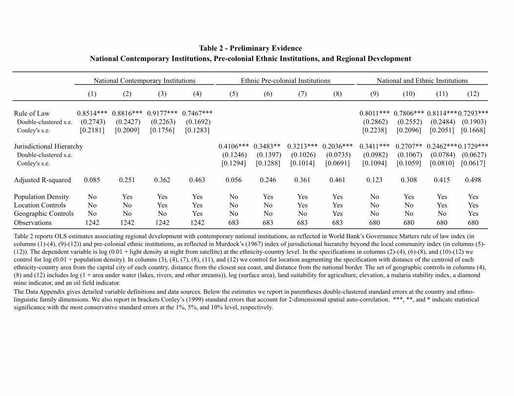
(1) (2) (3) (4) (5) (6) (7) (8) (9) (10) (11) (12)

Rule of Law 0.8514*** 0.8816*** 0.9177*** 0.7467*** 0.8011*** 0.7806*** 0.8114***0.7293*** Double-clustered s.e. (0.2743) (0.2427) (0.2263) (0.1692) (0.2862) (0.2552) (0.2484) (0.1903) Conley's s.e. [0.2181] [0.2009] [0.1756] [0.1283] [0.2238] [0.2096] [0.2051] [0.1668]

Jurisdictional Hierarchy 0.4106*** 0.3483** 0.3213*** 0.2036*** 0.3411*** 0.2707** 0.2462***0.1729*** Double-clustered s.e. (0.1246) (0.1397) (0.1026) (0.0735) (0.0982) (0.1067) (0.0784) (0.0627) Conley's s.e. [0.1294] [0.1288] [0.1014] [0.0691] [0.1094] [0.1059] [0.0810] [0.0617]

Adjusted R-squared 0.085 0.251 0.362 0.463 0.056 0.246 0.361 0.461 0.123 0.308 0.415 0.498

Population Density No Yes Yes Yes No Yes Yes Yes No Yes Yes YesLocation Controls No No Yes Yes No No Yes Yes No No Yes YesGeographic Controls No No No Yes No No No Yes No No No YesObservations 1242 1242 1242 1242 683 683 683 683 680 680 680 680

The Data Appendix gives detailed variable definitions and data sources. Below the estimates we report in parentheses double-clustered standard errors at the country and ethno-linguistic family dimensions. We also report in brackets Conley’s (1999) standard errors that account for 2-dimensional spatial auto-correlation. ***, **, and * indicate statistical significance with the most conservative standard errors at the 1%, 5%, and 10% level, respectively.

Table 2 reports OLS estimates associating regional development with contemporary national institutions, as reflected in World Bank’s Governance Matters rule of law index (in columns (1)-(4), (9)-(12)) and pre-colonial ethnic institutions, as reflected in Murdock’s (1967) index of jurisdictional hierarchy beyond the local community index (in columns (5)-(12)). The dependent variable is log (0.01 + light density at night from satellite) at the ethnicity-country level. In the specifications in columns (2)-(4), (6)-(8), and (10)-(12) we control for log (0.01 + population density). In columns (3), (4), (7), (8), (11), and (12) we control for location augmenting the specification with distance of the centroid of each ethnicity-country area from the capital city of each country, distance from the closest sea coast, and distance from the national border. The set of geographic controls in columns (4), (8) and (12) includes log (1 + area under water (lakes, rivers, and other streams)), log (surface area), land suitability for agriculture, elevation, a malaria stability index, a diamond mine indicator, and an oil field indicator.

Table 2 - Preliminary Evidence National Contemporary Institutions, Pre-colonial Ethnic Institutions, and Regional Development

National Contemporary Institutions Ethnic Pre-colonial Institutions National and Ethnic Institutions

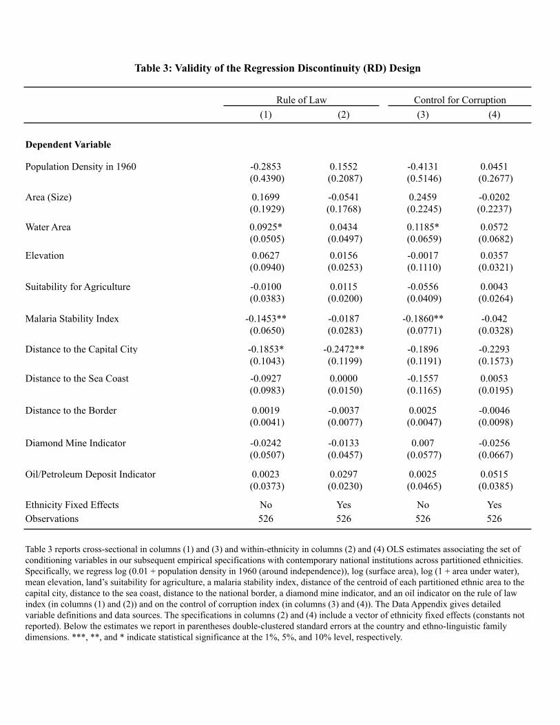
(1) (2) (3) (4)

Dependent Variable

Population Density in 1960 -0.2853 0.1552 -0.4131 0.0451 (0.4390) (0.2087) (0.5146) (0.2677)

Area (Size) 0.1699 -0.0541 0.2459 -0.0202 (0.1929) (0.1768) (0.2245) (0.2237)

Water Area 0.0925* 0.0434 0.1185* 0.0572 (0.0505) (0.0497) (0.0659) (0.0682)

Elevation 0.0627 0.0156 -0.0017 0.0357 (0.0940) (0.0253) (0.1110) (0.0321)

Suitability for Agriculture -0.0100 0.0115 -0.0556 0.0043 (0.0383) (0.0200) (0.0409) (0.0264)

Malaria Stability Index -0.1453** -0.0187 -0.1860** -0.042 (0.0650) (0.0283) (0.0771) (0.0328)

Distance to the Capital City -0.1853* -0.2472** -0.1896 -0.2293 (0.1043) (0.1199) (0.1191) (0.1573)

Distance to the Sea Coast -0.0927 0.0000 -0.1557 0.0053 (0.0983) (0.0150) (0.1165) (0.0195)

Distance to the Border 0.0019 -0.0037 0.0025 -0.0046 (0.0041) (0.0077) (0.0047) (0.0098)

Diamond Mine Indicator -0.0242 -0.0133 0.007 -0.0256 (0.0507) (0.0457) (0.0577) (0.0667)

Oil/Petroleum Deposit Indicator 0.0023 0.0297 0.0025 0.0515 (0.0373) (0.0230) (0.0465) (0.0385)

Ethnicity Fixed Effects No Yes No YesObservations 526 526 526 526

Table 3: Validity of the Regression Discontinuity (RD) Design

Table 3 reports cross-sectional in columns (1) and (3) and within-ethnicity in columns (2) and (4) OLS estimates associating the set of conditioning variables in our subsequent empirical specifications with contemporary national institutions across partitioned ethnicities. Specifically, we regress log (0.01 + population density in 1960 (around independence)), log (surface area), log (1 + area under water), mean elevation, land’s suitability for agriculture, a malaria stability index, distance of the centroid of each partitioned ethnic area to the capital city, distance to the sea coast, distance to the national border, a diamond mine indicator, and an oil indicator on the rule of law index (in columns (1) and (2)) and on the control of corruption index (in columns (3) and (4)). The Data Appendix gives detailed variable definitions and data sources. The specifications in columns (2) and (4) include a vector of ethnicity fixed effects (constants not reported). Below the estimates we report in parentheses double-clustered standard errors at the country and ethno-linguistic family dimensions. ***, **, and * indicate statistical significance at the 1%, 5%, and 10% level, respectively.

Rule of Law Control for Corruption

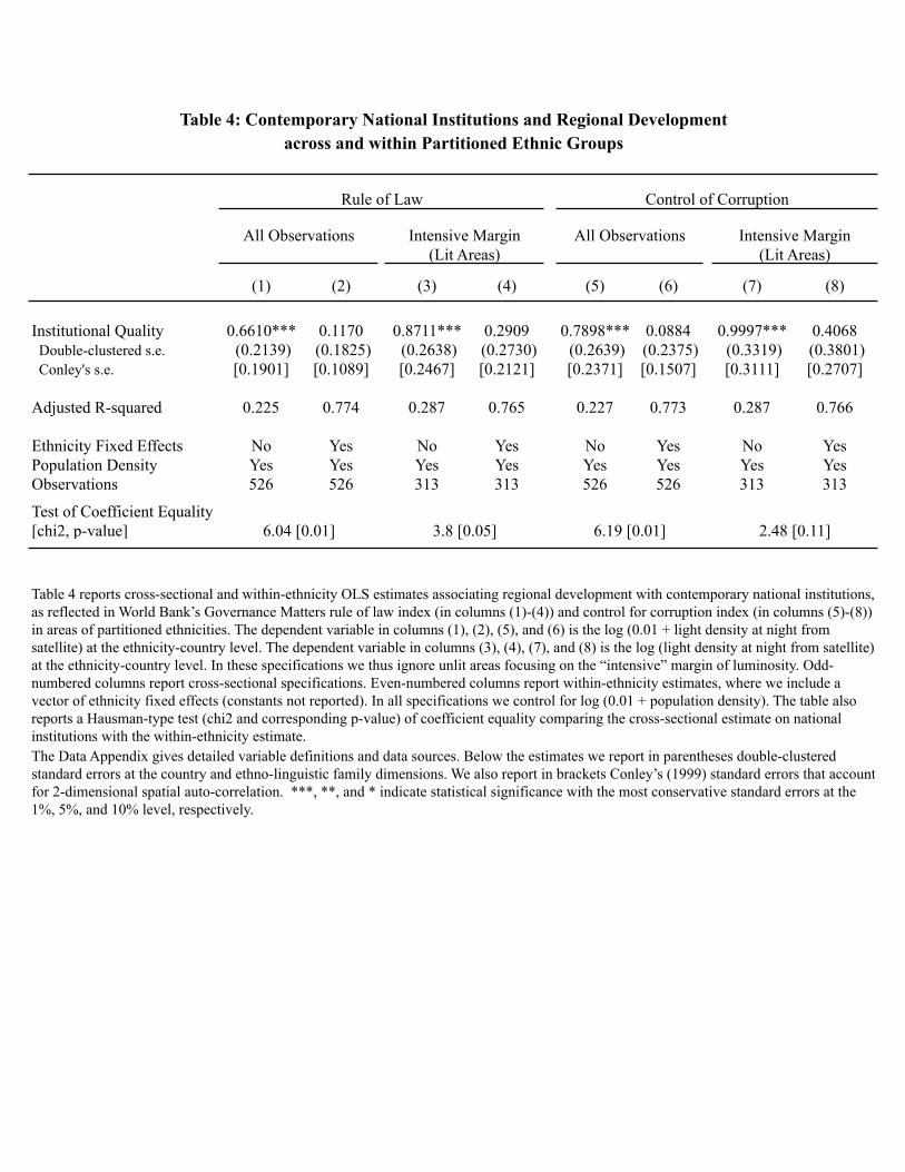
(1) (2) (3) (4) (5) (6) (7) (8)

Institutional Quality 0.6610*** 0.1170 0.8711*** 0.2909 0.7898*** 0.0884 0.9997*** 0.4068 Double-clustered s.e. (0.2139) (0.1825) (0.2638) (0.2730) (0.2639) (0.2375) (0.3319) (0.3801) Conley's s.e. [0.1901] [0.1089] [0.2467] [0.2121] [0.2371] [0.1507] [0.3111] [0.2707]

Adjusted R-squared 0.225 0.774 0.287 0.765 0.227 0.773 0.287 0.766

Ethnicity Fixed Effects No Yes No Yes No Yes No YesPopulation Density Yes Yes Yes Yes Yes Yes Yes YesObservations 526 526 313 313 526 526 313 313

Test of Coefficient Equality [chi2, p-value]

All Observations Intensive Margin (Lit Areas)

Rule of Law Control of Corruption

6.04 [0.01] 3.8 [0.05] 6.19 [0.01] 2.48 [0.11]

The Data Appendix gives detailed variable definitions and data sources. Below the estimates we report in parentheses double-clustered standard errors at the country and ethno-linguistic family dimensions. We also report in brackets Conley’s (1999) standard errors that account for 2-dimensional spatial auto-correlation. ***, **, and * indicate statistical significance with the most conservative standard errors at the 1%, 5%, and 10% level, respectively.

Table 4: Contemporary National Institutions and Regional Development across and within Partitioned Ethnic Groups

Table 4 reports cross-sectional and within-ethnicity OLS estimates associating regional development with contemporary national institutions, as reflected in World Bank’s Governance Matters rule of law index (in columns (1)-(4)) and control for corruption index (in columns (5)-(8)) in areas of partitioned ethnicities. The dependent variable in columns (1), (2), (5), and (6) is the log (0.01 + light density at night from satellite) at the ethnicity-country level. The dependent variable in columns (3), (4), (7), and (8) is the log (light density at night from satellite) at the ethnicity-country level. In these specifications we thus ignore unlit areas focusing on the “intensive” margin of luminosity. Odd-numbered columns report cross-sectional specifications. Even-numbered columns report within-ethnicity estimates, where we include a vector of ethnicity fixed effects (constants not reported). In all specifications we control for log (0.01 + population density). The table also reports a Hausman-type test (chi2 and corresponding p-value) of coefficient equality comparing the cross-sectional estimate on national institutions with the within-ethnicity estimate.

All Observations Intensive Margin (Lit Areas)

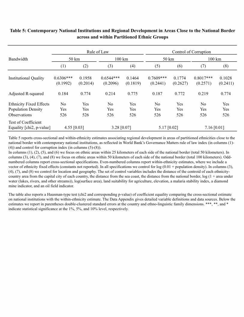
Bandwidth(1) (2) (3) (4) (5) (6) (7) (8)

Institutional Quality 0.6306*** 0.1958 0.6544*** 0.1464 0.7609*** 0.1774 0.8017*** 0.1028 (0.1992) (0.2014) (0.2096) (0.1819) (0.2441) (0.2627) (0.2571) (0.2411)

Adjusted R-squared 0.184 0.774 0.214 0.775 0.187 0.772 0.219 0.774

Ethnicity Fixed Effects No Yes No Yes No Yes No YesPopulation Density Yes Yes Yes Yes Yes Yes Yes YesObservations 526 526 526 526 526 526 526 526

Test of Coefficient Equality [chi2, p-value] 7.16 [0.01]

Table 5 reports cross-sectional and within-ethnicity estimates associating regional development in areas of partitioned ethnicities close to the national border with contemporary national institutions, as reflected in World Bank’s Governance Matters rule of law index (in columns (1)-(4)) and control for corruption index (in columns (5)-(8)).In columns (1), (2), (5), and (6) we focus on ethnic areas within 25 kilometers of each side of the national border (total 50 kilometers). In columns (3), (4), (7), and (8) we focus on ethnic areas within 50 kilometers of each side of the national border (total 100 kilometers). Odd-numbered columns report cross-sectional specifications. Even-numbered columns report within-ethnicity estimates, where we include a vector of ethnicity fixed effects (constants not reported). In all specifications we control for log (0.01 + population density). In columns (3), (4), (7), and (8) we control for location and geography. The set of control variables includes the distance of the centroid of each ethnicity-country area from the capital city of each country, the distance from the sea coast, the distance from the national border, log (1 + area under water (lakes, rivers, and other streams)), log(surface area), land suitability for agriculture, elevation, a malaria stability index, a diamond mine indicator, and an oil field indicator.

The table also reports a Hausman-type test (chi2 and corresponding p-value) of coefficient equality comparing the cross-sectional estimate on national institutions with the within-ethnicity estimate. The Data Appendix gives detailed variable definitions and data sources. Below the estimates we report in parentheses double-clustered standard errors at the country and ethno-linguistic family dimensions. ***, **, and * indicate statistical significance at the 1%, 5%, and 10% level, respectively.

4.55 [0.03] 3.28 [0.07] 5.17 [0.02]

50 km 100 km 50 km 100 km

Table 5: Contemporary National Institutions and Regional Development in Areas Close to the National Border across and within Partitioned Ethnic Groups

Rule of Law Control of Corruption

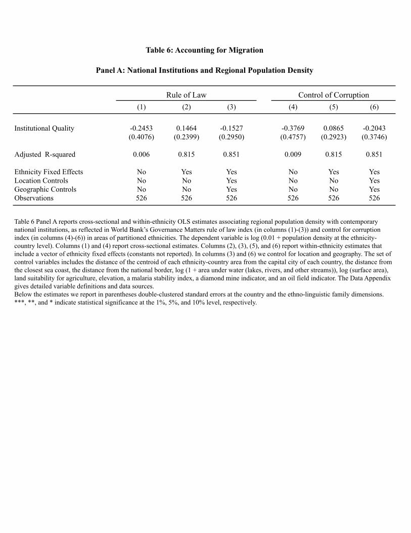
(1) (2) (3) (4) (5) (6)

Institutional Quality -0.2453 0.1464 -0.1527 -0.3769 0.0865 -0.2043(0.4076) (0.2399) (0.2950) (0.4757) (0.2923) (0.3746)

Adjusted R-squared 0.006 0.815 0.851 0.009 0.815 0.851

Ethnicity Fixed Effects No Yes Yes No Yes YesLocation Controls No No Yes No No YesGeographic Controls No No Yes No No YesObservations 526 526 526 526 526 526

Table 6: Accounting for Migration

Panel A: National Institutions and Regional Population Density

Table 6 Panel A reports cross-sectional and within-ethnicity OLS estimates associating regional population density with contemporary national institutions, as reflected in World Bank’s Governance Matters rule of law index (in columns (1)-(3)) and control for corruption index (in columns (4)-(6)) in areas of partitioned ethnicities. The dependent variable is log (0.01 + population density at the ethnicity-country level). Columns (1) and (4) report cross-sectional estimates. Columns (2), (3), (5), and (6) report within-ethnicity estimates that include a vector of ethnicity fixed effects (constants not reported). In columns (3) and (6) we control for location and geography. The set of control variables includes the distance of the centroid of each ethnicity-country area from the capital city of each country, the distance from the closest sea coast, the distance from the national border, log (1 + area under water (lakes, rivers, and other streams)), log (surface area), land suitability for agriculture, elevation, a malaria stability index, a diamond mine indicator, and an oil field indicator. The Data Appendix gives detailed variable definitions and data sources. Below the estimates we report in parentheses double-clustered standard errors at the country and the ethno-linguistic family dimensions. ***, **, and * indicate statistical significance at the 1%, 5%, and 10% level, respectively.

Rule of Law Control of Corruption

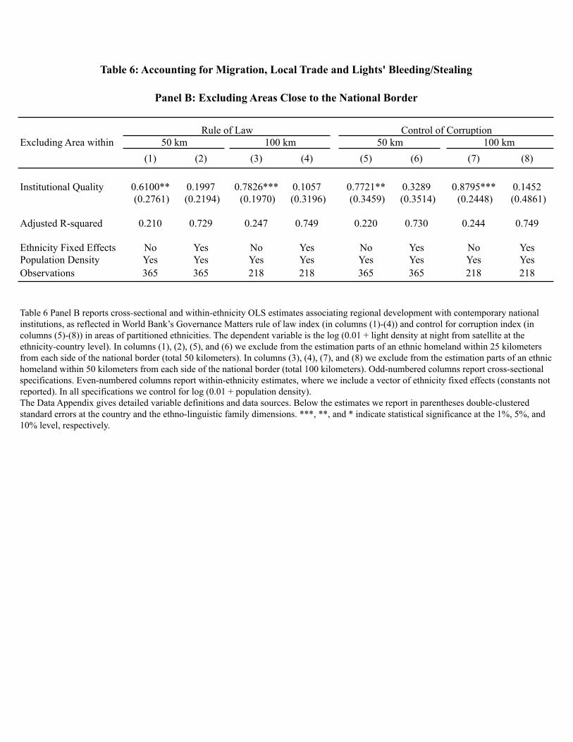
Excluding Area within(1) (2) (3) (4) (5) (6) (7) (8)

Institutional Quality 0.6100** 0.1997 0.7826*** 0.1057 0.7721** 0.3289 0.8795*** 0.1452 (0.2761) (0.2194) (0.1970) (0.3196) (0.3459) (0.3514) (0.2448) (0.4861)

Adjusted R-squared 0.210 0.729 0.247 0.749 0.220 0.730 0.244 0.749

Ethnicity Fixed Effects No Yes No Yes No Yes No YesPopulation Density Yes Yes Yes Yes Yes Yes Yes YesObservations 365 365 218 218 365 365 218 218

100 km Rule of Law Control of Corruption

The Data Appendix gives detailed variable definitions and data sources. Below the estimates we report in parentheses double-clustered standard errors at the country and the ethno-linguistic family dimensions. ***, **, and * indicate statistical significance at the 1%, 5%, and 10% level, respectively.

Table 6 Panel B reports cross-sectional and within-ethnicity OLS estimates associating regional development with contemporary national institutions, as reflected in World Bank’s Governance Matters rule of law index (in columns (1)-(4)) and control for corruption index (in columns (5)-(8)) in areas of partitioned ethnicities. The dependent variable is the log (0.01 + light density at night from satellite at the ethnicity-country level). In columns (1), (2), (5), and (6) we exclude from the estimation parts of an ethnic homeland within 25 kilometers from each side of the national border (total 50 kilometers). In columns (3), (4), (7), and (8) we exclude from the estimation parts of an ethnic homeland within 50 kilometers from each side of the national border (total 100 kilometers). Odd-numbered columns report cross-sectional specifications. Even-numbered columns report within-ethnicity estimates, where we include a vector of ethnicity fixed effects (constants not reported). In all specifications we control for log (0.01 + population density).

Table 6: Accounting for Migration, Local Trade and Lights' Bleeding/Stealing

Panel B: Excluding Areas Close to the National Border

50 km 100 km 50 km

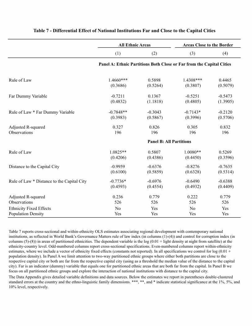
(1) (2) (3) (4)

Rule of Law 1.4660*** 0.5898 1.4308*** 0.4465 (0.3686) (0.5264) (0.3807) (0.5079)

Far Dummy Variable -0.7211 0.1367 -0.5251 -0.5473 (0.4832) (1.1818) (0.4805) (1.3905)

Rule of Law * Far Dummy Variable -0.7848** -0.3043 -0.7143* -0.2120 (0.3983) (0.5867) (0.3996) (0.5706)

Adjusted R-squared 0.327 0.826 0.305 0.832Observations 196 196 196 196

Rule of Law 1.0825** 0.5807 1.0080** 0.5269 (0.4206) (0.4386) (0.4450) (0.3596)

Distance to the Capital City -0.9959 -0.6376 -0.8276 -0.7635 (0.6100) (0.5859) (0.6328) (0.5314)

Rule of Law * Distance to the Capital City -0.7736* -0.6976 -0.6490 -0.6388 (0.4593) (0.4554) (0.4932) (0.4409)

Adjusted R-squared 0.236 0.779 0.222 0.779Observations 526 526 526 526Ethnicity Fixed Effects No Yes No YesPopulation Density Yes Yes Yes Yes

Panel A: Ethnic Partitions Both Close or Far from the Capital Cities

The Data Appendix gives detailed variable definitions and data sources. Below the estimates we report in parentheses double-clustered standard errors at the country and the ethno-linguistic family dimensions. ***, **, and * indicate statistical significance at the 1%, 5%, and 10% level, respectively.

Table 7 - Differential Effect of National Institutions Far and Close to the Capital Cities

All Ethnic Areas Areas Close to the Border

Table 7 reports cross-sectional and within-ethnicity OLS estimates associating regional development with contemporary national institutions, as reflected in World Bank’s Governance Matters rule of law index (in columns (1)-(4)) and control for corruption index (in columns (5)-(8)) in areas of partitioned ethnicities. The dependent variable is the log (0.01 + light density at night from satellite) at the ethnicity-country level. Odd-numbered columns report cross-sectional specifications. Even-numbered columns report within-ethnicity estimates, where we include a vector of ethnicity fixed effects (constants not reported). In all specifications we control for log (0.01 + population density). In Panel A we limit attention to two-way partitioned ethnic groups where either both partitions are close to the respective capital city or both are far from the respective capital city (using as a threshold the median value of the distance to the capital city). Far is an indicator (dummy) variable that equals one for partitioned ethnic areas that are both far from the capital. In Panel B we focus on all partitioned ethnic groups and explore the interaction of national institutions with distance to the capital city.

Panel B: All Partitions

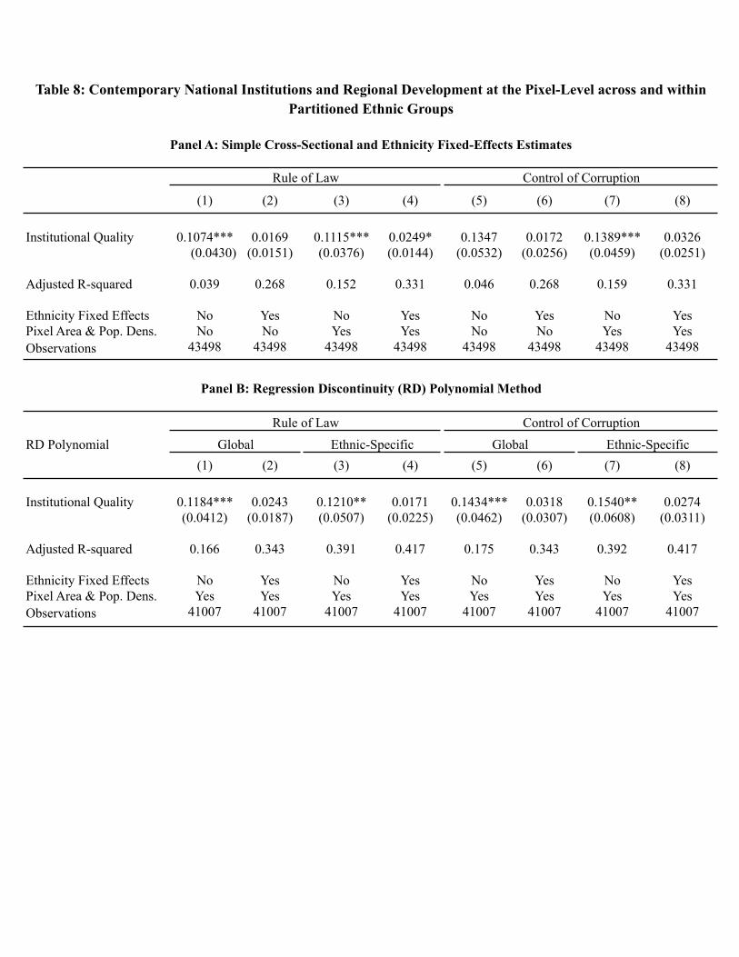
(1) (2) (3) (4) (5) (6) (7) (8)

Institutional Quality 0.1074*** 0.0169 0.1115*** 0.0249* 0.1347 0.0172 0.1389*** 0.0326(0.0430) (0.0151) (0.0376) (0.0144) (0.0532) (0.0256) (0.0459) (0.0251)

Adjusted R-squared 0.039 0.268 0.152 0.331 0.046 0.268 0.159 0.331

Ethnicity Fixed Effects No Yes No Yes No Yes No YesPixel Area & Pop. Dens. No No Yes Yes No No Yes YesObservations 43498 43498 43498 43498 43498 43498 43498 43498

RD Polynomial(1) (2) (3) (4) (5) (6) (7) (8)

Institutional Quality 0.1184*** 0.0243 0.1210** 0.0171 0.1434*** 0.0318 0.1540** 0.0274(0.0412) (0.0187) (0.0507) (0.0225) (0.0462) (0.0307) (0.0608) (0.0311)

Adjusted R-squared 0.166 0.343 0.391 0.417 0.175 0.343 0.392 0.417

Ethnicity Fixed Effects No Yes No Yes No Yes No YesPixel Area & Pop. Dens. Yes Yes Yes Yes Yes Yes Yes YesObservations 41007 41007 41007 41007 41007 41007 41007 41007

Panel B: Regression Discontinuity (RD) Polynomial Method

Global Ethnic-Specific Global Ethnic-Specific

Panel A: Simple Cross-Sectional and Ethnicity Fixed-Effects Estimates

Rule of Law Control of Corruption

Table 8: Contemporary National Institutions and Regional Development at the Pixel-Level across and within Partitioned Ethnic Groups

Rule of Law Control of Corruption

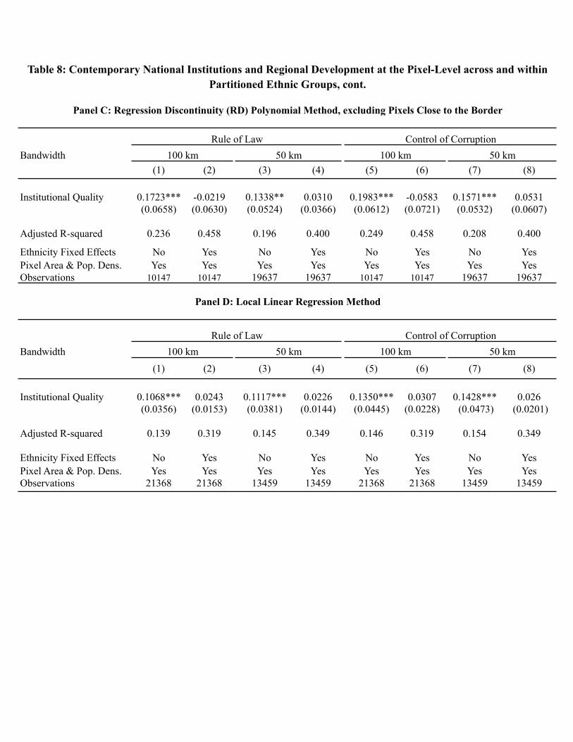
Bandwidth(1) (2) (3) (4) (5) (6) (7) (8)

Institutional Quality 0.1723*** -0.0219 0.1338** 0.0310 0.1983*** -0.0583 0.1571*** 0.0531(0.0658) (0.0630) (0.0524) (0.0366) (0.0612) (0.0721) (0.0532) (0.0607)

Adjusted R-squared 0.236 0.458 0.196 0.400 0.249 0.458 0.208 0.400

Ethnicity Fixed Effects No Yes No Yes No Yes No YesPixel Area & Pop. Dens. Yes Yes Yes Yes Yes Yes Yes YesObservations 10147 10147 19637 19637 10147 10147 19637 19637

Bandwidth(1) (2) (3) (4) (5) (6) (7) (8)

Institutional Quality 0.1068*** 0.0243 0.1117*** 0.0226 0.1350*** 0.0307 0.1428*** 0.026(0.0356) (0.0153) (0.0381) (0.0144) (0.0445) (0.0228) (0.0473) (0.0201)

Adjusted R-squared 0.139 0.319 0.145 0.349 0.146 0.319 0.154 0.349

Ethnicity Fixed Effects No Yes No Yes No Yes No YesPixel Area & Pop. Dens. Yes Yes Yes Yes Yes Yes Yes YesObservations 21368 21368 13459 13459 21368 21368 13459 13459

Panel C: Regression Discontinuity (RD) Polynomial Method, excluding Pixels Close to the Border

100 km 50 kmControl of Corruption

100 km

Rule of Law Control of Corruption

Rule of Law

100 km 50 km 100 km 50 km

Panel D: Local Linear Regression Method

50 km

Table 8: Contemporary National Institutions and Regional Development at the Pixel-Level across and within Partitioned Ethnic Groups, cont.

Table 8 - Notes

The Data Appendix gives detailed variable definitions and data sources. Below the estimates we report in parentheses double-clustered standard errors at the country and at the ethnicity level dimensions. ***, **, and * indicate statistical significance at the 1%, 5%, and 10% level, respectively.

Panel A reports cross-sectional and ethnicity fixed-effects specifications. Panel B reports RD-specifications with a polynomial control function. Estimation is performed across the two major partitions of each ethnic group. In columns (1), (2), (5), and (6) we include a (global) third-order RD polynomial in distance of the centroid of each pixel to the national border; distance takes positive values for pixels that belong to the relatively high institutional quality country and negative values for pixels that fall in the relatively low institutional quality country. The specifications also include interactions between the polynomial terms and the proxy measure of national institutions. In columns (3), (4), (7), and (8) we include ethnicity-specific third-order RD polynomial terms in distance of the centroid of each pixel to the national border; for each ethnicity separately distance takes positive values for pixels that belong to the relatively high institutional quality country and negative values for pixels that fall in the relatively low institutional quality country. The specifications also include interactions between the ethnicity-specific polynomial terms and the proxy measure of national institutions.Panel C reports RD-specifications with a global polynomial control function on distance to the national border. Estimation is performed across the two major partitions of each ethnic group. In columns (1), (2), (5), and (6) we exclude from the estimation pixels within 50 kilometers from each side of the national border (total 100 kilometers). In columns (3), (4), (7), and (8) we exclude from the estimation the parts of an ethnic homeland within 25 kilometers from each side of the national border (total 50 kilometers). Panel D reports RD-specifications with a local linear regression method restricting estimation in pixels close to the national border. Estimation is performed across the two major partitions of each ethnic group. In columns (1), (2), (5), and (6) we focus on pixels within 50 kilometers on each side of the national border (total 100 kilometers). In columns (3), (4), (7), and (8) we focus on pixels within 25 kilometers of each side of the national border (total 50 kilometers).

All panels of Table 8 report cross-sectional and within-ethnicity OLS estimates associating regional development, as reflected in satellite light density at night, with contemporary national institutions, as reflected in World Bank’s Governance Matters rule of law index (in columns (1)-(4)) and control for corruption index (in columns (5)-(8)). The unit of analysis is pixels of 0.125 x 0.125 decimal degrees (around 12 x 12 kilometers) within partitioned ethnicities. The dependent variable in all specifications is a dummy variable that takes the value one if the pixel is lit and zero otherwise. Even-numbered specifications report within-ethnicity estimates that include a vector of ethnicity fixed effects (constants not reported). In Panel A, columns (3), (4), (7), and (8) and all specifications in Panel B, Panel C, and Panel D we control for the log (area) and log (population density) of each pixel.

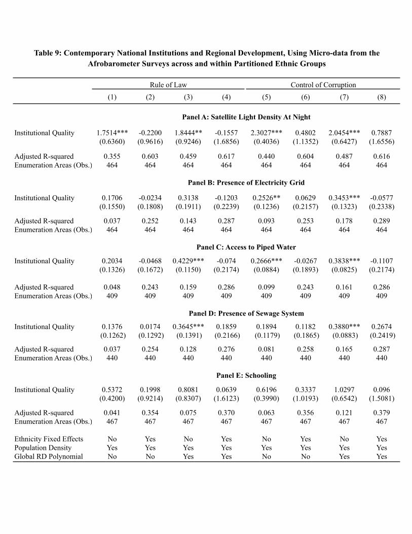
(1) (2) (3) (4) (5) (6) (7) (8)

Institutional Quality 1.7514*** -0.2200 1.8444** -0.1557 2.3027*** 0.4802 2.0454*** 0.7887(0.6360) (0.9616) (0.9246) (1.6856) (0.4036) (1.1352) (0.6427) (1.6556)

Adjusted R-squared 0.355 0.603 0.459 0.617 0.440 0.604 0.487 0.616Enumeration Areas (Obs.) 464 464 464 464 464 464 464 464

Institutional Quality 0.1706 -0.0234 0.3138 -0.1203 0.2526** 0.0629 0.3453*** -0.0577(0.1550) (0.1808) (0.1911) (0.2239) (0.1236) (0.2157) (0.1323) (0.2338)

Adjusted R-squared 0.037 0.252 0.143 0.287 0.093 0.253 0.178 0.289Enumeration Areas (Obs.) 464 464 464 464 464 464 464 464

Institutional Quality 0.2034 -0.0468 0.4229*** -0.074 0.2666*** -0.0267 0.3838*** -0.1107(0.1326) (0.1672) (0.1150) (0.2174) (0.0884) (0.1893) (0.0825) (0.2174)

Adjusted R-squared 0.048 0.243 0.159 0.286 0.099 0.243 0.161 0.286Enumeration Areas (Obs.) 409 409 409 409 409 409 409 409

Institutional Quality 0.1376 0.0174 0.3645*** 0.1859 0.1894 0.1182 0.3880*** 0.2674 (0.1262) (0.1292) (0.1391) (0.2166) (0.1179) (0.1865) (0.0883) (0.2419)

Adjusted R-squared 0.037 0.254 0.128 0.276 0.081 0.258 0.165 0.287Enumeration Areas (Obs.) 440 440 440 440 440 440 440 440

Institutional Quality 0.5372 0.1998 0.8081 0.0639 0.6196 0.3337 1.0297 0.096(0.4200) (0.9214) (0.8307) (1.6123) (0.3990) (1.0193) (0.6542) (1.5081)

Adjusted R-squared 0.041 0.354 0.075 0.370 0.063 0.356 0.121 0.379Enumeration Areas (Obs.) 467 467 467 467 467 467 467 467

Ethnicity Fixed Effects No Yes No Yes No Yes No YesPopulation Density Yes Yes Yes Yes Yes Yes Yes YesGlobal RD Polynomial No No Yes Yes No No Yes Yes

Panel D: Presence of Sewage System

Table 9: Contemporary National Institutions and Regional Development, Using Micro-data from the Afrobarometer Surveys across and within Partitioned Ethnic Groups

Panel A: Satellite Light Density At Night

Panel B: Presence of Electricity Grid

Panel C: Access to Piped Water

Panel E: Schooling

Rule of Law Control of Corruption

Table 9 - Notes

The specifications also include the interactions between the polynomial terms and the proxy measure of national institutions. In Panel A the dependent variable is average light density in a radius of 10 km from the centroid of an Afrobarometer’s enumeration area. In Panel B the dependent variable is the average within an Afrobarometer’s enumeration area of respondent’s answer on "whether in the enumeration area there is an electricity grid that most houses could access". In Panel C the dependent variable is the average within an Afrobarometer’s enumeration area of respondent’s answer on "whether in the enumeration area there is a piped water system that most houses could access". In Panel D the dependent variable is the average within an Afrobarometer’s enumeration area of respondent’s answer on "whether in the enumeration area there is a sewage system that most houses could access". In Panel E the dependent variable is the average years of schooling across respondents within each Afrobarometer’s enumeration area. In all specifications we control for ln (0.01 + population density in a 10km radius of the enumeration area). In all specifications we control for ln(0.01 + population density).

The Data Appendix gives detailed variable definitions and data sources. Appendix Table 1 – Panel A gives summary statistics for all variables from the 2005 Afrobarometer Surveys. Below the estimates we report in parentheses double-clustered standard errors at the country and at the ethnicity level dimensions. ***, **, and * indicate statistical significance at the 1%, 5%, and 10% level, respectively.

All panels of Table 9 report cross-sectional and within-ethnicity OLS estimates associating regional development, as reflected in satellite images on light density at night, public goods provision, and education, with contemporary national institutions, as reflected in World Bank’s Governance Matters rule of law index (in columns (1)-(4)) and control for corruption index (in columns (5)-(8)) in areas of partitioned ethnicities. The unit of analysis is an enumeration area of the 2005 Afrobarometer Surveys. As within each enumeration area there are several households, we average household responses within the enumeration area and use the respective averages as the dependent variable. Odd-numbered specifications report cross-sectional estimates. Even-numbered specifications report within-ethnicity estimates that include a vector of ethnicity fixed effects (constants not reported). In columns (3), (4), (7), and (8) we include a (global) third-order RD polynomial in distance of each enumeration area to the national border; distance takes positive values for areas that belong to the relatively high institutional quality country and negative values for partitioned areas that fall in the relatively low institutional quality country.

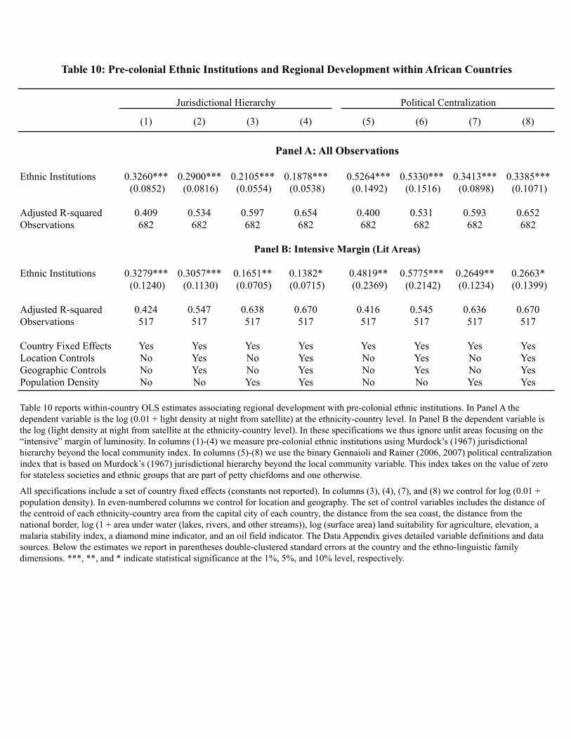
(1) (2) (3) (4) (5) (6) (7) (8)

Ethnic Institutions 0.3260*** 0.2900*** 0.2105*** 0.1878*** 0.5264*** 0.5330*** 0.3413*** 0.3385*** (0.0852) (0.0816) (0.0554) (0.0538) (0.1492) (0.1516) (0.0898) (0.1071)

Adjusted R-squared 0.409 0.534 0.597 0.654 0.400 0.531 0.593 0.652Observations 682 682 682 682 682 682 682 682

Ethnic Institutions 0.3279*** 0.3057*** 0.1651** 0.1382* 0.4819** 0.5775*** 0.2649** 0.2663* (0.1240) (0.1130) (0.0705) (0.0715) (0.2369) (0.2142) (0.1234) (0.1399)

Adjusted R-squared 0.424 0.547 0.638 0.670 0.416 0.545 0.636 0.670Observations 517 517 517 517 517 517 517 517

Country Fixed Effects Yes Yes Yes Yes Yes Yes Yes YesLocation Controls No Yes No Yes No Yes No YesGeographic Controls No Yes No Yes No Yes No YesPopulation Density No No Yes Yes No No Yes Yes

Panel B: Intensive Margin (Lit Areas)

Table 10 reports within-country OLS estimates associating regional development with pre-colonial ethnic institutions. In Panel A the dependent variable is the log (0.01 + light density at night from satellite) at the ethnicity-country level. In Panel B the dependent variable is the log (light density at night from satellite at the ethnicity-country level). In these specifications we thus ignore unlit areas focusing on the “intensive” margin of luminosity. In columns (1)-(4) we measure pre-colonial ethnic institutions using Murdock’s (1967) jurisdictional hierarchy beyond the local community index. In columns (5)-(8) we use the binary Gennaioli and Rainer (2006, 2007) political centralization index that is based on Murdock’s (1967) jurisdictional hierarchy beyond the local community variable. This index takes on the value of zero for stateless societies and ethnic groups that are part of petty chiefdoms and one otherwise.

Panel A: All Observations

All specifications include a set of country fixed effects (constants not reported). In columns (3), (4), (7), and (8) we control for log (0.01 + population density). In even-numbered columns we control for location and geography. The set of control variables includes the distance of the centroid of each ethnicity-country area from the capital city of each country, the distance from the sea coast, the distance from the national border, log (1 + area under water (lakes, rivers, and other streams)), log (surface area) land suitability for agriculture, elevation, a malaria stability index, a diamond mine indicator, and an oil field indicator. The Data Appendix gives detailed variable definitions and data sources. Below the estimates we report in parentheses double-clustered standard errors at the country and the ethno-linguistic family dimensions. ***, **, and * indicate statistical significance at the 1%, 5%, and 10% level, respectively.

Table 10: Pre-colonial Ethnic Institutions and Regional Development within African Countries

Jurisdictional Hierarchy Political Centralization

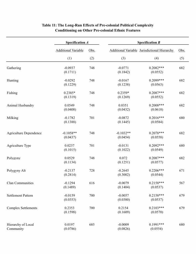
Additional Variable Obs. Additional Variable Jurisdictional Hierarchy Obs.

(1) (2) (3) (4) (5)

Gathering -0.0937 748 -0.0771 0.2082*** 682 (0.1711) (0.1842) (0.0552)

Hunting -0.0292 748 -0.0167 0.2099*** 682 (0.1229) (0.1238) (0.0563)

Fishing 0.2385* 748 0.2359* 0.2087*** 682 (0.1319) (0.1269) (0.0552)

Animal Husbandry 0.0549 748 0.0351 0.2008*** 682 (0.0408) (0.0432) (0.0618)

Milking -0.1782 701 -0.0872 0.2016*** 680 (0.1388) (0.1445) (0.0584)

Agriculture Dependence -0.1058** 748 -0.1032** 0.2078*** 682 (0.0437) (0.0454) (0.0558)

Agriculture Type 0.0237 701 -0.0131 0.2092*** 680 (0.1015) (0.1022) (0.0549)

Polygyny 0.0529 748 0.072 0.2087*** 682 (0.1134) (0.1251) (0.0577)

Polygyny Alt -0.2137 728 -0.2645 0.2206*** 671 (0.2814) (0.3002) (0.0544)

Clan Communities -0.1294 616 -0.0079 0.2158*** 567(0.1489) (0.1404) (0.0537)

Settlement Pattern -0.0159 700 -0.0057 0.2158*** 679 (0.0353) (0.0380) (0.0537)

Complex Settlements 0.2353 700 0.2154 0.2103*** 679 (0.1598) (0.1609) (0.0570)

Hierarchy of Local 0.0197 685 -0.0009 0.1991*** 680Community (0.0786) (0.0826) (0.0554)

Specification A Specification B

Table 11: The Long-Run Effects of Pre-colonial Political Complexity Conditioning on Other Pre-colonial Ethnic Features

Patrilineal Descent -0.1880 732 -0.2011 0.1932*** 671 (0.1314) (0.1309) (0.0500)

Class Stratification 0.1268** 607 0.0672 0.1556** 570 (0.0494) (0.0581) (0.0697)

Class Stratification Indicator 0.3970** 607 0.2757 0.1441** 570 (0.1819) (0.1900) (0.0563)

Elections 0.3459 535 0.2764 0.2217*** 500 (0.2463) (0.2583) (0.0583)

Slavery 0.0962 665 0.0556 0.1801*** 616 (0.0613) (0.0581) (0.0591)

Property Rights -0.1963 568 -0.1788 0.2196*** 529(0.2173) (0.2283) (0.0691)

Table 11 reports within-country OLS estimates associating regional development with pre-colonial ethnic features as reflected in Murdock’s (1967) Ethnographic Atlas. The dependent variable is the log (0.01 + light density at night from satellite) at the ethnicity-country level. All specifications include a set of country fixed effects (constants not reported). In all specifications we control for log (0.01 + population density at the ethnicity-country level). In specification A (in columns (1)-(2)) we regress log (0.01 + light density) on various ethnic traits from Murdock (1967). In specification B (columns (3)-(5)) we regress log (0.01 + light density) on each of Murdock’s additional variables and the jurisdictional hierarchy beyond the local community index. The Data Appendix gives detailed variable definitions and data sources. Below the estimates we report in parentheses double-clustered standard errors at the country and the ethno-linguistic family dimensions. ***, **, and * indicate statistical significance at the 1%, 5%, and 10% level respectively.

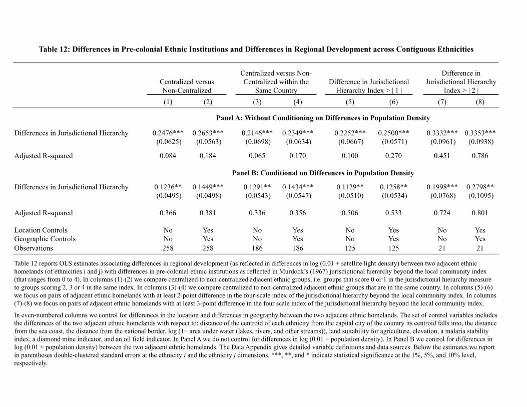
(1) (2) (3) (4) (5) (6) (7) (8)

Differences in Jurisdictional Hierarchy 0.2476*** 0.2653*** 0.2146*** 0.2349*** 0.2252*** 0.2500*** 0.3332*** 0.3353*** (0.0625) (0.0563) (0.0698) (0.0634) (0.0667) (0.0571) (0.0961) (0.0938)

Adjusted R-squared 0.084 0.184 0.065 0.170 0.100 0.270 0.451 0.786

Differences in Jurisdictional Hierarchy 0.1236** 0.1449*** 0.1291** 0.1434*** 0.1129** 0.1258** 0.1998*** 0.2798** (0.0495) (0.0498) (0.0543) (0.0547) (0.0510) (0.0534) (0.0768) (0.1095)

Adjusted R-squared 0.366 0.381 0.336 0.356 0.506 0.533 0.724 0.801

Location Controls No Yes No Yes No Yes No YesGeographic Controls No Yes No Yes No Yes No YesObservations 258 258 186 186 125 125 21 21

In even-numbered columns we control for differences in the location and differences in geography between the two adjacent ethnic homelands. The set of control variables includes the differences of the two adjacent ethnic homelands with respect to: distance of the centroid of each ethnicity from the capital city of the country its centroid falls into, the distance from the sea coast, the distance from the national border, log (1+ area under water (lakes, rivers, and other streams)), land suitability for agriculture, elevation, a malaria stability index, a diamond mine indicator, and an oil field indicator. In Panel A we do not control for differences in log (0.01 + population density). In Panel B we control for differences in log (0.01 + population density) between the two adjacent ethnic homelands. The Data Appendix gives detailed variable definitions and data sources. Below the estimates we report in parentheses double-clustered standard errors at the ethnicity i and the ethnicity j dimensions. ***, **, and * indicate statistical significance at the 1%, 5%, and 10% level, respectively.

Table 12 reports OLS estimates associating differences in regional development (as reflected in differences in log (0.01 + satellite light density) between two adjacent ethnic homelands (of ethnicities i and j) with differences in pre-colonial ethnic institutions as reflected in Murdock’s (1967) jurisdictional hierarchy beyond the local community index (that ranges from 0 to 4). In columns (1)-(2) we compare centralized to non-centralized adjacent ethnic groups, i.e. groups that score 0 or 1 in the jurisdictional hierarchy measure to groups scoring 2, 3 or 4 in the same index. In columns (3)-(4) we compare centralized to non-centralized adjacent ethnic groups that are in the same country. In columns (5)-(6) we focus on pairs of adjacent ethnic homelands with at least 2-point difference in the four-scale index of the jurisdictional hierarchy beyond the local community index. In columns (7)-(8) we focus on pairs of adjacent ethnic homelands with at least 3-point difference in the four scale index of the jurisdictional hierarchy beyond the local community index.

Panel A: Without Conditioning on Differences in Population Density

Panel B: Conditional on Differences in Population Density

Table 12: Differences in Pre-colonial Ethnic Institutions and Differences in Regional Development across Contiguous Ethnicities

Centralized versus Non-Centralized

Centralized versus Non-Centralized within the

Same CountryDifference in Jurisdictional

Hierarchy Index > | 1 |

Difference in Jurisdictional Hierarchy

Index > | 2 |

(1) (2) (3) (4) (5) (6)

0.0678*** 0.0530*** 0.0309*** 0.0464*** 0.0352*** 0.0380***(0.0227) (0.0190) (0.0116) (0.0179) (0.0117) (0.0086)

Adjusted R-squared 0.035 0.104 0.210 0.269 0.317 0.330

0.3601*** 0.2894*** 0.1730*** 0.2429** 0.1886*** 0.2131***(0.1256) (0.1048) (0.0621) (0.0984) (0.0659) (0.0498)

Adjusted R-squared 0.045 0.118 0.258 0.314 0.367 0.391

Observations 64330 64330 64330 64330 64330 64330Country Fixed Effects No No No Yes Yes YesPixel Area & Pop. Dens. No Yes Yes No Yes YesAdditional Controls No No Yes No No Yes

The specifications in columns (4)-(6) include a vector of country fixed effects (constants not reported). The Data Appendix gives detailed variable definitions and data sources. Below the estimates we report in parentheses double-clustered standard errors at the country and at the ethnicity level dimensions. ***, **, and * indicate statistical significance at the 1%, 5%, and 10% level, respectively.

Table 13: Precolonial Ethnic Institutions and Regional Development - Pixel Level Analysis

Jurisdictional Hierarchy beyond the Local Community

Table 13 reports cross-sectional and within-country OLS estimates associating regional development, as reflected in satellite light density at night with pre-colonial ethnic institutions, as reflected in Murdock’s (1967) jurisdictional hierarchy beyond the local community index. The unit of analysis is a pixel of 0.125 x 0.125 decimal degrees (around 12 x 12 kilometers). In Panel A the dependent variable is a dummy variable that takes on the value of one if the pixel is lit and zero otherwise. In Panel B the dependent variable is the log (0.01 + light density at night from satellite). In columns (2), (3), (5), and (6) we control for ln (pixel population density) and ln (pixel area). In columns (3) and (6) we control for the distance of the ethnicity-country’s centroid from the capital city of each country, the distance from the sea coast, the distance from the national border, ln (1 + area under water (lakes, rivers, and other streams)), land suitability for agriculture, elevation, a malaria stability index, a diamond mine indicator, and an oil field indicator.

Panel A: Lit/Unlit Pixels

Panel B: Ln (0.01 + Luminosity)

Jurisdictional Hierarchy beyond the Local Community

Cross-Sectional Estimates Within-Country Estimates

(1) (2) (3) (4) (5) (6)

0.0304** 0.0196* 0.0440** 0.0311*** 0.0461** 0.0339**(0.0145) (0.0109) (0.0216) (0.0157) (0.0229) (0.0157)

Adjusted R-squared 0.2778 0.3123 0.3507 0.3867 0.3163 0.3577Observations 27199 27199 15553 15553 9182 9182

Contiguous Ethnicity FE Yes Yes Yes Yes Yes YesPixel Area & Pop. Dens. No Yes No Yes No Yes

Table 14 reports adjacent ethnicity (pair) fixed-effects OLS estimates associating regional development, as reflected in satellite light density at night with pre-colonial ethnic institutions, as reflected in Murdock’s (1967) jurisdictional hierarchy beyond the local community index within pairs of adjacent ethnicities with a different degree of political centralization. The unit of analysis is a pixel of 0.125 x 0.125 decimal degrees (around 12 x 12 kilometers). Every pixel falls into the historical homeland of an ethnicity that is adjacent to the homeland of another ethnicity (where the two ethnicities score differently in the jurisdictional hierarchy beyond the local community index). The dependent variable is a dummy variable that takes on the value of one if the pixel is lit and zero otherwise. In columns (3)-(4) we restrict estimation to pixels of adjacent ethnic pairs that fall in the same country. In columns (5)-(6) we restrict estimation to pixels of adjacent ethnic pairs with large differences in the 0-4 jurisdictional hierarchy beyond the local level index (greater than one point) that fall in the same country. In even-numbered columns we control for ln (pixel population density) and ln (pixel area). Below the estimates we report in parentheses double-clustered standard errors at the country and at the ethnicity level dimensions. ***, **, and * indicate statistical significance at the 1%, 5%, and 10% level, respectively.

Table 14: Precolonial Ethnic Institutions and Regional Development - Pixel Level Analysis within Contiguous Ethnic Homelands

All ObservationsObservations within the Same

CountryDifference in Jurisdictional

Hierarchy Index > | 1 |

Jurisdictional Hierarchy beyond the Local Community

(1) (2) (3) (4) (5) (6)

0.0389* 0.0314* 0.0550** 0.0460** 0.0537** 0.0468** (0.0229) (0.0187) (0.0269) (0.0197) (0.0267) (0.0195)

Adjusted R-squared 0.2494 0.2851 0.3263 0.3619 0.3284 0.3664Observations 21895 21895 11746 11746 7049 7049

0.0561** 0.0453** 0.0816** 0.0674*** 0.0810** 0.0676***(0.0259) (0.0211) (0.0329) (0.0241) (0.0267) (0.0195)

Adjusted R-squared 0.2320 0.2684 0.3076 0.3454 0.3171 0.3571Observations 19209 19209 9923 9923 5988 5988

0.0658** 0.0533** 0.0983*** 0.0798*** 0.0889** 0.0715**(0.0264) (0.0211) (0.0355) (0.0256) (0.0387) (0.0280)

Adjusted R-squared 0.2155 0.2518 0.2859 0.3244 0.3110 0.3525Observations 16584 16584 8210 8210 5003 5003

Contiguous Ethnicity FE Yes Yes Yes Yes Yes YesPixel Area & Pop. Dens. No Yes No Yes No Yes

Table 15: Precolonial Ethnic Institutions and Regional Development - Pixel Level Analysis across Contiguous Ethnic Homelands

All ObservationsObservations within the

Same CountryDifference in Jurisdictional

Hierarchy Index > | 1 |

RD Specifications

In columns (3)-(4) we restrict estimation to pixels of adjacent ethnic pairs that fall in the same country. In columns (5)-(6) we restrict estimation to pixels of adjacent ethnic pairs with large differences in the 0-4 jurisdictional hierarchy beyond the local level index (greater than one point) that fall in the same country. In even-numbered columns we control for ln (pixel population density) and ln (pixel area). Below the estimates we report in parentheses double-clustered standard errors at the country and at the ethnicity level dimensions. ***, **, and * indicate statistical significance at the 1%, 5%, and 10% level, respectively.

All specifications include a (global) third-order RD polynomial on distance of the centroid of each pixel to the ethnic border; distance takes positive values for pixels that belong to the homeland of the politically centralized ethnicities and negative values for pixels that fall in the politically non-centralized ones. The specifications also include interactions between the polynomial terms and the jurisdictional hierarchy beyond the local level index. To account for population mixing in the areas along the ethnic boundary, measurement error on the exact separating line between the two ethnicities, and bleeding in the luminosity data we exclude from the estimation areas very close to the ethnic border (i.e. we assume a “thick” border and estimate the distance of each pixel to this “thick” border). In Panel A we exclude areas 50km from each side of the ethnic border (total 100km). In Panel B we exclude areas 75km from each side of the ethnic border (total 150km). In Panel C we exclude areas 100km from each side of the ethnic border (total 200km).

Panel A: Discontituity at 50 km from Each Side of the Ethnic Border

Jurisdictional Hierarchy beyond the Local Community

Panel C: Discontituity at 100 km from Each Side of the Ethnic Border

Panel B: Discontituity at 75 km from Each Side of the Ethnic Border

Jurisdictional Hierarchy beyond the Local Community

Jurisdictional Hierarchy beyond the Local Community

Table 15 reports RD (regression discontinuity) estimates with a polynomial control function. All Panels report adjacent ethnicity (pair) fixed-effects OLS estimates associating regional development, as reflected in satellite light density at night with pre-colonial ethnic institutions, as reflected in Murdock’s (1967) jurisdictional hierarchy beyond the local community index within pairs of adjacent ethnicities with a different degree of political centralization. The unit of analysis is a pixel of 0.125 x 0.125 decimal degrees (around 12 x 12 kilometers). Every pixel falls into the historical homeland of an ethnicity that is adjacent to the homeland of another ethnicity (where the two ethnicities score differently in the jurisdictional hierarchy beyond the local community index). The dependent variable is a dummy variable that takes on the value of one if the pixel is lit and zero otherwise.