Embed Size (px)
Citation preview
Distribution Consolidation and Pricing in the Beer Industry
Anton Popov
August 25, 2019
Abstract
This paper studies consolidation of distributors in the beer industry and its interaction with
the uniform pricing by retailers. I build a theoretical model which illustrates how distributor
consolidation in a set of counties may affect retail prices in all counties, depending on how
strong the incentive of retail chains to price uniformly is. Empirically, using Nielsen scanner
price data, I study two events of distributor consolidation in Ohio in 2009–2011, which followed
upstream MillerCoors joint venture in 2008. In one of the events, distributor consolidation has
no price effects. In another, bigger event, prices of consolidated brands (Miller, Coors, Heineken
and Modelo) in treated counties increase by 0.46% relative to the control ABI brands. I find
no evidence of prices in other counties being affected. The findings are consistent with some
regimes of my theoretical model. The implications of this study are that modeling distribution
tier and uniform pricing by retailers may be important for horizontal merger practitioners, both
in retrospect and for forecasting.
1 Introduction
Horizontal merger analysis, a central tool in anti-trust enforcement, often abstracts away from
the vertical structure of the industry by assuming that each firm sets the final price for its
product (e.g., Nevo (2001), Miller and Weinberg (2017)). The analysis resulting from such
assumptions may be limited in two ways. First, consolidation upstream may be followed by
consolidation downstream. Both predicted and actual price increases due to consolidation up-
stream may be mismeasured if one does not include distributor consolidation in the analysis.
Second, interactions of pricing incentives in different distribution tiers may affect the predicted
upward pricing pressure following the merger. For example, retail supermarket chains often
price uniformly in most of their stores (DellaVigna and Gentzkow (2017)). Abstracting away
from this aspect may bias the merger counterfactuals.
1
This paper studies consolidation of beer distributors, which followed the upstream merger of
Miller and Coors in 2008. I show theoretically that distributor consolidation may have effects
on retail prices either in only counties which were treated by consolidation, or in all counties,
depending on how strong the incentive of retailers to price uniformly is. I test empirically both
hypotheses for two events of distributor consolidation in my data. I find support for higher
prices of consolidated brands in treated counties for one of the events. I find no evidence for
higher prices in all counties. Thus, in this empirical setting uniform pricing by retailers does
not have interactions with distributor consolidation. However, the latter does have an effect on
prices, which was missed by the previous studies.
In many US states beer distribution system is three-tiered, with big manufactures only being
able to sell to retailers through distributors. Moreover, some states require exclusive territories
of distribution, effectively giving a distributor monopoly power in its territories. For any beer
brand, the manufacturer needs to divide the state into non-overlapping territories, such that in
any territory only one distributor has the right to sell the brand. This is the case for Ohio state,
which I study in this paper.
Before 2008 some territories in Ohio had Miller and Coors brands sold by separate distribu-
tors. After the merger MillerCoors tried to consolidate their distribution network by switching
Miller brands to distributors of Coors, or vice versa, with two successful attempts. If distrib-
utors have pricing power in this market, such consolidation may let the distributor internalize
the pricing externality, raising wholesale prices, which may reflect in retail price increases for
consolidated brands in treated territories. However, this effect may not be observed if the chains
adopt uniform pricing across territories. Incentives of chains to price uniformly may over-weigh
the upward pricing pressure in any particular store affected by distributor consolidation. Still,
if a consolidated distributor has some additional pricing power, this upward pricing pressure in
a set of territories may manifest in a higher overall pricing level of a uniformly pricing retail
chain.
I start by outlining a stylized model, in which these ideas are formalized. I introduce a penalty
term in the profit function of the monopolist retailer, which reflects the desire of retailer to price
uniformly. The penalty term includes a parameter, which governs how strong uniform pricing
incentive is. I give numerical examples of solutions to a two-stage game where distributors set
wholesale prices first, and a retailer, operating in multiple counties, sets its prices second. I
show that when two distributors of different brands merge in one of the counties, there exist
two types of equilibria: one where it leads to retail price increases only in counties treated
by consolidation, and another where it leads to price increases in all counties. The type of
equilibrium depends on the uniform pricing parameter: naturally, when this parameter is low,
the first type of equilibrium is realized, and when it is high, the second.
2
I continue with a descriptive analysis of pricing by several retail chains in Ohio. I use Nielsen
scanner data from 2009–2011 to show that many chains are pricing uniformly, with 80% of stores
in a given chain setting exactly the same price for a specific beer product for prolonged periods
of time.
Having established the existence of uniform pricing at the retail level, I continue by studying
two events of distributor consolidation. In one of these events, in December 2009, distribution
of Miller brands by Metropolitan distributing company in 6 counties was discontinued, with the
brands transferred to Bonbright Distributors in 3 counties, and the Fisher Company in another 3
counties. Both Bonbright Distributors and Fisher Company were distributors of Coors, Corona
and Heineken at the end of the sample in 2011. In the second event, in June 2010, Kerr
Distributing and Kerr Wholesale, which were distributing Coors brands in 17 counties, were
acquired by AFP Distributors, carrying Miller, Corona and Heineken, in all but one of these
counties. Thus, both of these events led to consolidation of Miller, Coors, Corona and Heineken
brands in the hands of one distributor, whereas before the event one of the brands (either Miller
or Coors) was not consolidated with the other three. I call the counties where the consolidation
events happened “treatment” counties, and all the other counties “control”. The group of
brands which, following the events, was consolidated in the hands of one distributor (Miller,
Coors, Corona and Heineken) are “consolidated” brands, and ABI brands, which were sold by
separate distributors, are “control” brands.
The main contribution of this paper is to study empirically the pricing effects of these two
distribution consolidation events. Using the retail prices from Nielsen data as the main outcome,
I study two hypotheses. First, in the treatment counties consolidated brands may see higher
price increases than non-consolidated brands.1 I use counties not treated by distribution consoli-
dation as control counties. Thus, this hypothesis requires a triple difference approach, where the
coefficient of interest is given by an interaction on (post distributor consolidation)×(treatment
county)×(consolidated brand). Controlling for non-consolidated brands accounts for the marginal
cost shocks which were common to consolidated and non-consolidated brands at the time
of event. Controlling for counties not treated by distribution consolidation accounts for the
marginal cost shocks which were common across the state of Ohio for a given brand, for exam-
ple, at the manufacturer level. Differential marginal cost shocks on both of these dimensions
(brand and geography), coincidental with the timing of consolidation event, may be a problem
for identification of the effect.
To explain the second hypothesis, it is useful to consider whether rejection of the first hy-
pothesis proves that distributors have no pricing power. In the setting where retail chains price
uniformly, it may be the case that in response to a wholesale price increase by a consolidated
1As a standard horizontal merger analysis would suggest.
3
distributor in the treatment counties, the retail chain finds it optimal to increase prices in all
counties, not only the ones where a distributor consolidated. The presence of such price in-
crease, common to all stores of a chain, constitutes the second hypothesis which I test. The
relevant coefficient comes from the double difference approach, on interaction of (post distribu-
tor consolidation)×(consolidated brand). Again, non-consolidated brands here are the control
group, which accounts for the marginal cost shocks coincidental with the consolidation event,
common to all brewers. There are no control counties here, because under the null hypothesis
all counties raise prices by the same amount for consolidated brands, and by the same (different)
amount for control brands.
The empirical results of this study are as follows. For the first hypothesis I find no price
increases during event 1, contemporaneously or in the following 15 months. There is also no
contemporaneous price increase for event 2. However, there is a price effect 9 months after event
2, with consolidated brands increasing prices by 0.51% more in the treated counties. This effect
is statistically significant, with the 95% confidence interval of [0.13%, 0.88%]. My interpretation
of this first set of findings is that the distributors have some degree of pricing power. When
consolidation affects more counties, as is the case with event 2, the incentive of retail chains to
price optimally in those counties seems to over-weigh the incentive to price uniformly. On the
other hand, event 1 only affects 6 counties, so the cost of keeping non-optimal uniform price
may not be high in that case. The lagged impact of distributor consolidation may be due to
rigidity of contracts. The second hypothesis that the distributor consolidation can affect pricing
in all counties does not find support in either of two consolidation events. Intuitively, for this
effect to exist both the uniform pricing incentive of retail chains and the upward pricing pressure
created by the distributor consolidation need to be high. Then it could be optimal to increase
prices in all counties where a retail chain operates, passing through the upward pricing pressure
from treatment counties to all counties. However, given that the price effect (as estimated by
hypothesis 1 testing) is not too high, it is reasonable that the second hypothesis finds no support.
Related literature
This paper is related to a wide range of research on the beer markets. The first group of papers
estimates the effects from the MillerCoors merger itself. Ashenfelter, Hosken, and Weinberg
(2015) compare upward pricing pressure resulting from the merger to cost efficiencies which it
generated by allowing Miller to brew their beers in Coors plants and vice versa, reducing shipping
costs. Using a reduced form approach, they find that increased concentration would raise prices
by 2% on average, but the cost efficiencies offset this price increase. A later paper by Miller
and Weinberg (2017) estimates the coordination parameter between joint MillerCoors and ABI,
4
using a structural model of demand and supply. They conclude that the merger increased the
amount of coordination between MillerCoors and ABI, which led to higher price increases than
what could be anticipated in the absence of coordination effects. The price increases related to
coordination effects are around 6–8 percentage points. It is the presence of coordination effects
which eroded the benefits coming from the cost efficiencies of the merger.
The second group of papers explore effects of exclusive territories on the beer markets. Sass
and Saurman (1996) study Indiana’s 1979 ban on the grant of exclusive territories. By studying
effects of the ban on quantities and prices of beer sold, they empirically estimate if the monopoly
power that exclusive territories give has an overall positive impact. Theoretically it could be bad
for price competition, but good for promoting the optimal dealer effort. Exclusive territories
ban is estimated to have reduced both consumption and prices of beer, leading the authors to
conclude that exclusive territories do increase demand through better dealer services. Burgdorf
(2019) studies a reverse event, where in 2006 Wisconsin required the brewers to assign exclusive
territories to their distributors. He finds that following the new mandate prices of craft beer
went up and quantity decreased. The conclusion is that the exclusive territories caused an
increase in the distribution cost, especially for the craft beer manufacturers.
Asker (2016) considers a different kind of exclusivity. Some distributors work exclusively with
a single manufacturer. In the US this is almost always the case for ABI distributors, whereas
other manufacturers may or may not share distributors. Asker (2016) studies the presence of
foreclosure effects in the markets where Miller uses an exclusive distributor as opposed to the
markets where Miller distributor also carries other brands. Using data on retail beer prices
and quantities in Dominick’s Finer Foods in Illinois in 1994, he estimates a structural model
of the industry and backs out costs and demand effects related to facing a Miller-exclusive
distributor. He does not find any evidence that the competing distributors have higher costs or
lower demand when Miller signs an exclusive contract with one of the distributors, thus rejecting
the foreclosure hypothesis.
What is common to the structural papers on beer markets mentioned above (Miller and
Weinberg (2017) and Asker (2016)) is that in their main specifications they do not model
distributors as price-setting, effectively assuming that the distributors only cover their fixed
costs, and do not contribute to double marginalization. Asker (2016) mentions the institutional
setting in Illinois which justifies such an approach: “The brewer has varying degrees of input
into the wholesale price charged by the distributor to retailers. When dealing with a large
supermarket chain, a sales representative from the brewer will arrive at a wholesale price for
the chain with the chain’s buyer. Distributors are then expected to supply at that price. While
resale price maintenance is prohibited explicitly by the Beer Industry Fair Trading Act... this
practice does not appear to invite legal sanction.”
5
There is also theoretical research laying out a different argument for lack of double marginal-
ization in markets like this. Bernheim and Whinston (1985) show that when a downstream firm
works with multiple upstream firms, the monopolistic outcome may be achieved. Effectively the
upstream firms “sell out” their business to a single agent downstream. Theoretically, incentives
described by Bernheim and Whinston (1985) could be present in the beer markets where a single
distributor may serve multiple brewers in an overlapping set of exclusive territories.
My paper serves as an empirical test to whether distributors have no pricing power, as in
Asker (2016) and (most of) Miller and Weinberg (2017). I reject this conjecture for one of
distributor consolidation effects which I study, showing that it did increase retail prices. Notice
that this finding does not, however, reject the model laid out in Bernheim and Whinston (1985).
Indeed, if consolidation leads from three brands being consolidated to four, and Bernheim and
Whinston (1985) predict a monopolistic price in both cases, under standard assumptions the
distributor will set a higher wholesale price when it has four brands consolidated than when it
has three.
The finding that distribution structure matters for retail pricing is an important one both
for studying mergers in the past and modeling mergers under review. For example, one of the
assumptions in Miller and Weinberg (2017) is that MillerCoors, both pre- and post-merger, had
a zero coordination parameter with Heineken and Modelo (brewer of Corona). However, as I
show here, there are price effects related to MillerCoors, Heineken and Modelo being sold by
the same distributor. What the model in Miller and Weinberg (2017) would attribute to pure
unilateral effects of Nash competition between MillerCoors and Heineken/Modelo, may instead
be picking up some of the joint distribution effects, overestimating the magnitude of unilateral
effects. If the true unilateral effects are smaller than what Miller and Weinberg (2017) estimate,
the coordination effects may in reality be even higher.
Finally, this paper is related to the study of uniform pricing by US supermarket chains
in DellaVigna and Gentzkow (2017). They document that despite big variations in consumer
demographics and competition across multiple locations of supermarket chains, they charge
nearly uniform prices for a range of products, including beer. My paper presents similar evidence
of uniform pricing for beer by chains in the state of Ohio.
The rest of the paper is structured as follows. Section 2 lays out a theoretical model, section
3 describes the data, section 4 shows evidence of uniform pricing by chains, section 5 presents
my empirical estimates, section 6 discusses the results, and section 7 concludes.
6
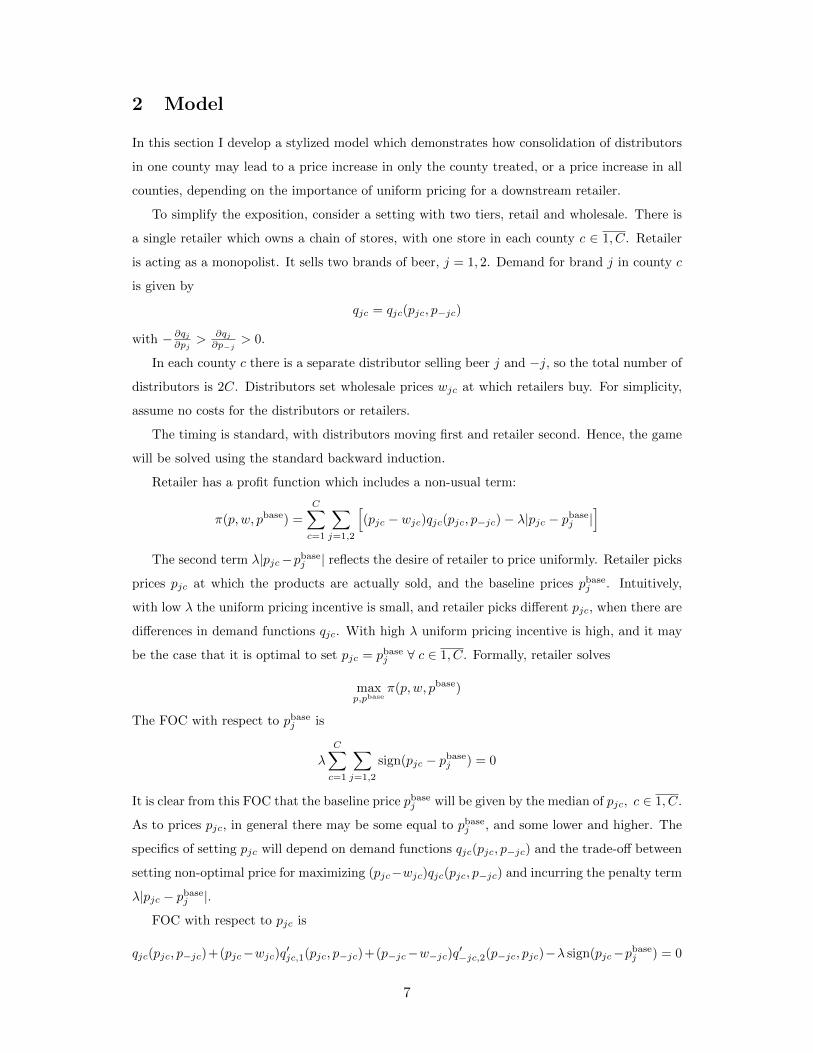
2 Model
In this section I develop a stylized model which demonstrates how consolidation of distributors
in one county may lead to a price increase in only the county treated, or a price increase in all
counties, depending on the importance of uniform pricing for a downstream retailer.
To simplify the exposition, consider a setting with two tiers, retail and wholesale. There is
a single retailer which owns a chain of stores, with one store in each county c ∈ 1, C. Retailer
is acting as a monopolist. It sells two brands of beer, j = 1, 2. Demand for brand j in county c
is given by
qjc = qjc(pjc, p−jc)
with − ∂qj∂pj
>∂qj∂p−j
> 0.
In each county c there is a separate distributor selling beer j and −j, so the total number of
distributors is 2C. Distributors set wholesale prices wjc at which retailers buy. For simplicity,
assume no costs for the distributors or retailers.
The timing is standard, with distributors moving first and retailer second. Hence, the game
will be solved using the standard backward induction.
Retailer has a profit function which includes a non-usual term:
π(p, w, pbase) =
C∑c=1
∑j=1,2
[(pjc − wjc)qjc(pjc, p−jc)− λ|pjc − pbasej |
]The second term λ|pjc−pbasej | reflects the desire of retailer to price uniformly. Retailer picks
prices pjc at which the products are actually sold, and the baseline prices pbasej . Intuitively,
with low λ the uniform pricing incentive is small, and retailer picks different pjc, when there are
differences in demand functions qjc. With high λ uniform pricing incentive is high, and it may
be the case that it is optimal to set pjc = pbasej ∀ c ∈ 1, C. Formally, retailer solves
maxp,pbase
π(p, w, pbase)
The FOC with respect to pbasej is
λ
C∑c=1
∑j=1,2
sign(pjc − pbasej ) = 0
It is clear from this FOC that the baseline price pbasej will be given by the median of pjc, c ∈ 1, C.
As to prices pjc, in general there may be some equal to pbasej , and some lower and higher. The
specifics of setting pjc will depend on demand functions qjc(pjc, p−jc) and the trade-off between
setting non-optimal price for maximizing (pjc−wjc)qjc(pjc, p−jc) and incurring the penalty term
λ|pjc − pbasej |.
FOC with respect to pjc is
qjc(pjc, p−jc)+(pjc−wjc)q′jc,1(pjc, p−jc)+(p−jc−w−jc)q′−jc,2(p−jc, pjc)−λ sign(pjc−pbasej ) = 0
7
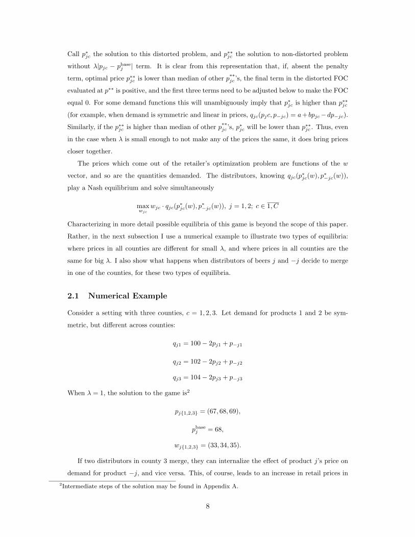
Call p∗jc the solution to this distorted problem, and p∗∗jc the solution to non-distorted problem
without λ|pjc − pbasej | term. It is clear from this representation that, if, absent the penalty
term, optimal price p∗∗jc is lower than median of other p**jc ’s, the final term in the distorted FOC
evaluated at p∗∗ is positive, and the first three terms need to be adjusted below to make the FOC
equal 0. For some demand functions this will unambiguously imply that p∗jc is higher than p∗∗jc
(for example, when demand is symmetric and linear in prices, qjc(pjc, p−jc) = a+ bpjc−dp−jc).
Similarly, if the p∗∗jc is higher than median of other p**jc ’s, p∗jc will be lower than p∗∗jc . Thus, even
in the case when λ is small enough to not make any of the prices the same, it does bring prices
closer together.
The prices which come out of the retailer’s optimization problem are functions of the w
vector, and so are the quantities demanded. The distributors, knowing qjc(p∗jc(w), p∗−jc(w)),
play a Nash equilibrium and solve simultaneously
maxwjc
wjc · qjc(p∗jc(w), p∗−jc(w)), j = 1, 2; c ∈ 1, C
Characterizing in more detail possible equilibria of this game is beyond the scope of this paper.
Rather, in the next subsection I use a numerical example to illustrate two types of equilibria:
where prices in all counties are different for small λ, and where prices in all counties are the
same for big λ. I also show what happens when distributors of beers j and −j decide to merge
in one of the counties, for these two types of equilibria.
2.1 Numerical Example
Consider a setting with three counties, c = 1, 2, 3. Let demand for products 1 and 2 be sym-
metric, but different across counties:
qj1 = 100− 2pj1 + p−j1
qj2 = 102− 2pj2 + p−j2
qj3 = 104− 2pj3 + p−j3
When λ = 1, the solution to the game is2
pj{1,2,3} = (67, 68, 69),
pbasej = 68,
wj{1,2,3} = (33, 34, 35).
If two distributors in county 3 merge, they can internalize the effect of product j’s price on
demand for product −j, and vice versa. This, of course, leads to an increase in retail prices in
2Intermediate steps of the solution may be found in Appendix A.
8
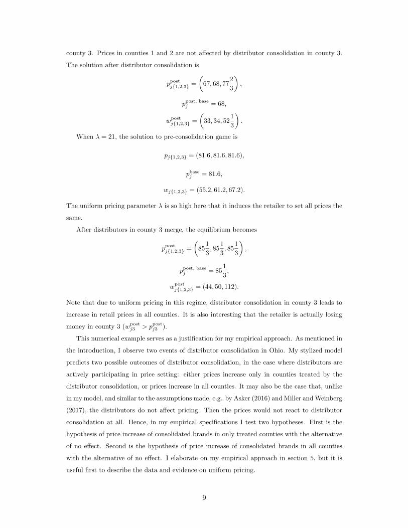
county 3. Prices in counties 1 and 2 are not affected by distributor consolidation in county 3.
The solution after distributor consolidation is
ppostj{1,2,3} =
(67, 68, 77
2
3
),
ppost, basej = 68,
wpostj{1,2,3} =
(33, 34, 52
1
3
).
When λ = 21, the solution to pre-consolidation game is
pj{1,2,3} = (81.6, 81.6, 81.6),
pbasej = 81.6,
wj{1,2,3} = (55.2, 61.2, 67.2).
The uniform pricing parameter λ is so high here that it induces the retailer to set all prices the
same.
After distributors in county 3 merge, the equilibrium becomes
ppostj{1,2,3} =
(85
1
3, 85
1
3, 85
1
3
),
ppost, basej = 851
3,
wpostj{1,2,3} = (44, 50, 112).
Note that due to uniform pricing in this regime, distributor consolidation in county 3 leads to
increase in retail prices in all counties. It is also interesting that the retailer is actually losing
money in county 3 (wpostj3 > ppostj3 ).
This numerical example serves as a justification for my empirical approach. As mentioned in
the introduction, I observe two events of distributor consolidation in Ohio. My stylized model
predicts two possible outcomes of distributor consolidation, in the case where distributors are
actively participating in price setting: either prices increase only in counties treated by the
distributor consolidation, or prices increase in all counties. It may also be the case that, unlike
in my model, and similar to the assumptions made, e.g. by Asker (2016) and Miller and Weinberg
(2017), the distributors do not affect pricing. Then the prices would not react to distributor
consolidation at all. Hence, in my empirical specifications I test two hypotheses. First is the
hypothesis of price increase of consolidated brands in only treated counties with the alternative
of no effect. Second is the hypothesis of price increase of consolidated brands in all counties
with the alternative of no effect. I elaborate on my empirical approach in section 5, but it is
useful first to describe the data and evidence on uniform pricing.
9
3 Data
The data come from two sources. The first is Nielsen scanner data. These are weekly data on
quantity sold and average price at the UPC level from multiple store chains that Nielsen tracks.
There are two well-known caveats of the scanner data. First, it records only products that had
a unit sold in any given week. If there are no sales of a UPC in a given week, it could be because
the store was out of this product, or because the product was on the shelf, but nobody bought
it. This first issue may lead to high prices missing in the data for some stores with low demand
(it may be that a store is more likely to not have a product sold when its price is high). Since
the big chains in my data will have a sale of all major products in all weeks, I do not consider
this to be a big issue.3 The second caveat is that the prices may change mid-week. This is not
an issue for my reduced form empirical specifications, which are run on these weekly average
prices taken directly from the data.
The second data set is the information on beer distributors, brands they are carrying, and
their territories from the Ohio Division of Liquor Control. These data for years 2009 to 2011
come in paper form as the scans from the Division of Liquor Control archives. Ideally I would
like to know the changes in the distribution structure in the year of the MillerCoors merger
(2008), as well. Unfortunately, the forms in that period are not very reliable, so I resort to
studying the period following the merger.
In the next subsections I describe each part of the data in more detail.
3.1 Brands
To have some consistency with the previous literature, I restrict attention to the same brands
as Miller and Weinberg (2017). These are 13 flagship brands of ABI, Miller, Coors, Heineken
and Modelo, which account for 40% of revenue of all beers in the Nielsen data.
The data have information at the UPC level, but for the purposes of exposition and empirical
analysis it may be useful to aggregate the data. In my regressions I fix the product level at
brand–(packaging size)–(unit size) combination. An example of a product would be Miller 12-
pack of 12 oz. units. If it is sold both in bottles and cans, such UPCs are aggregated into one
product.
Summary statistics on brands at even more aggregated brand level are shown in Table 1.4
Units and prices here are normalized to a 144-oz equivalent unit to be able to aggregate different
products of a given brand into a meaningful statistic.5 The time period that I use in this study
3Although I admit that the inclusion of smaller chains for which this is more likely to happen could bias the
relevant coefficients down, if the issue is more pronounced for treatment group than for control.4Table 9 in the Appendix shows summary statistics at the product level.5Also following Miller and Weinberg (2017).
10
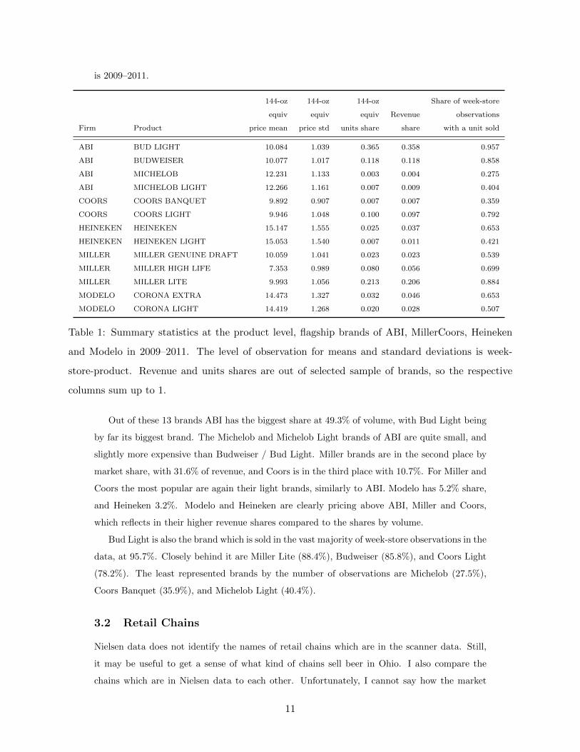
is 2009–2011.
144-oz 144-oz 144-oz Share of week-store
equiv equiv equiv Revenue observations
Firm Product price mean price std units share share with a unit sold
ABI BUD LIGHT 10.084 1.039 0.365 0.358 0.957
ABI BUDWEISER 10.077 1.017 0.118 0.118 0.858
ABI MICHELOB 12.231 1.133 0.003 0.004 0.275
ABI MICHELOB LIGHT 12.266 1.161 0.007 0.009 0.404
COORS COORS BANQUET 9.892 0.907 0.007 0.007 0.359
COORS COORS LIGHT 9.946 1.048 0.100 0.097 0.792
HEINEKEN HEINEKEN 15.147 1.555 0.025 0.037 0.653
HEINEKEN HEINEKEN LIGHT 15.053 1.540 0.007 0.011 0.421
MILLER MILLER GENUINE DRAFT 10.059 1.041 0.023 0.023 0.539
MILLER MILLER HIGH LIFE 7.353 0.989 0.080 0.056 0.699
MILLER MILLER LITE 9.993 1.056 0.213 0.206 0.884
MODELO CORONA EXTRA 14.473 1.327 0.032 0.046 0.653
MODELO CORONA LIGHT 14.419 1.268 0.020 0.028 0.507
Table 1: Summary statistics at the product level, flagship brands of ABI, MillerCoors, Heineken
and Modelo in 2009–2011. The level of observation for means and standard deviations is week-
store-product. Revenue and units shares are out of selected sample of brands, so the respective
columns sum up to 1.
Out of these 13 brands ABI has the biggest share at 49.3% of volume, with Bud Light being
by far its biggest brand. The Michelob and Michelob Light brands of ABI are quite small, and
slightly more expensive than Budweiser / Bud Light. Miller brands are in the second place by
market share, with 31.6% of revenue, and Coors is in the third place with 10.7%. For Miller and
Coors the most popular are again their light brands, similarly to ABI. Modelo has 5.2% share,
and Heineken 3.2%. Modelo and Heineken are clearly pricing above ABI, Miller and Coors,
which reflects in their higher revenue shares compared to the shares by volume.
Bud Light is also the brand which is sold in the vast majority of week-store observations in the
data, at 95.7%. Closely behind it are Miller Lite (88.4%), Budweiser (85.8%), and Coors Light
(78.2%). The least represented brands by the number of observations are Michelob (27.5%),
Coors Banquet (35.9%), and Michelob Light (40.4%).
3.2 Retail Chains
Nielsen data does not identify the names of retail chains which are in the scanner data. Still,
it may be useful to get a sense of what kind of chains sell beer in Ohio. I also compare the
chains which are in Nielsen data to each other. Unfortunately, I cannot say how the market
11
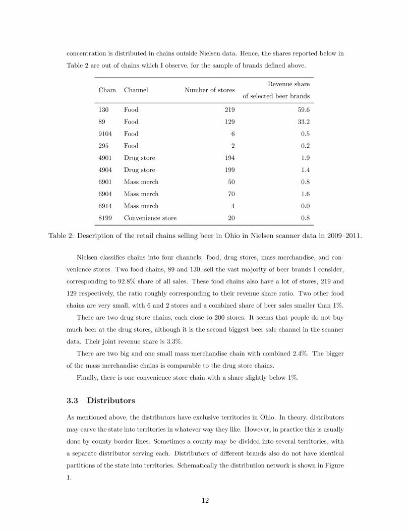
concentration is distributed in chains outside Nielsen data. Hence, the shares reported below in
Table 2 are out of chains which I observe, for the sample of brands defined above.
Chain Channel Number of storesRevenue share
of selected beer brands
130 Food 219 59.6
89 Food 129 33.2
9104 Food 6 0.5
295 Food 2 0.2
4901 Drug store 194 1.9
4904 Drug store 199 1.4
6901 Mass merch 50 0.8
6904 Mass merch 70 1.6
6914 Mass merch 4 0.0
8199 Convenience store 20 0.8
Table 2: Description of the retail chains selling beer in Ohio in Nielsen scanner data in 2009–2011.
Nielsen classifies chains into four channels: food, drug stores, mass merchandise, and con-
venience stores. Two food chains, 89 and 130, sell the vast majority of beer brands I consider,
corresponding to 92.8% share of all sales. These food chains also have a lot of stores, 219 and
129 respectively, the ratio roughly corresponding to their revenue share ratio. Two other food
chains are very small, with 6 and 2 stores and a combined share of beer sales smaller than 1%.
There are two drug store chains, each close to 200 stores. It seems that people do not buy
much beer at the drug stores, although it is the second biggest beer sale channel in the scanner
data. Their joint revenue share is 3.3%.
There are two big and one small mass merchandise chain with combined 2.4%. The bigger
of the mass merchandise chains is comparable to the drug store chains.
Finally, there is one convenience store chain with a share slightly below 1%.
3.3 Distributors
As mentioned above, the distributors have exclusive territories in Ohio. In theory, distributors
may carve the state into territories in whatever way they like. However, in practice this is usually
done by county border lines. Sometimes a county may be divided into several territories, with
a separate distributor serving each. Distributors of different brands also do not have identical
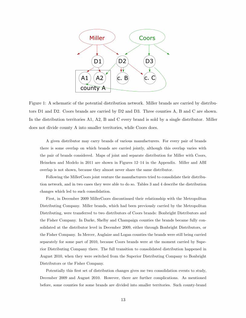
partitions of the state into territories. Schematically the distribution network is shown in Figure
1.
12
Miller Coors
D1 D2 D3
A2A1 c. B c. C
county A
Figure 1: A schematic of the potential distribution network. Miller brands are carried by distribu-
tors D1 and D2. Coors brands are carried by D2 and D3. Three counties A, B and C are shown.
In the distribution territories A1, A2, B and C every brand is sold by a single distributor. Miller
does not divide county A into smaller territories, while Coors does.
A given distributor may carry brands of various manufacturers. For every pair of brands
there is some overlap on which brands are carried jointly, although this overlap varies with
the pair of brands considered. Maps of joint and separate distribution for Miller with Coors,
Heineken and Modelo in 2011 are shown in Figures 12–14 in the Appendix. Miller and ABI
overlap is not shown, because they almost never share the same distributor.
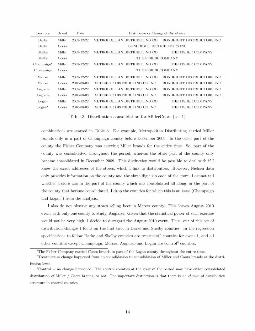
Following the MillerCoors joint venture the manufacturers tried to consolidate their distribu-
tion network, and in two cases they were able to do so. Tables 3 and 4 describe the distribution
changes which led to such consolidation.
First, in December 2009 MillerCoors discontinued their relationship with the Metropolitan
Distributing Company. Miller brands, which had been previously carried by the Metropolitan
Distributing, were transferred to two distributors of Coors brands: Bonbright Distributors and
the Fisher Company. In Darke, Shelby and Champaign counties the brands became fully con-
solidated at the distributor level in December 2009, either through Bonbright Distributors, or
the Fisher Company. In Mercer, Auglaize and Logan counties the brands were still being carried
separately for some part of 2010, because Coors brands were at the moment carried by Supe-
rior Distributing Company there. The full transition to consolidated distribution happened in
August 2010, when they were switched from the Superior Distributing Company to Bonbright
Distributors or the Fisher Company.
Potentially this first set of distribution changes gives me two consolidation events to study,
December 2009 and August 2010. However, there are further complications. As mentioned
before, some counties for some brands are divided into smaller territories. Such county-brand
13
Territory Brand Date Distributor or Change of Distributor
Darke Miller 2009-12-22 METROPOLITAN DISTRIBUTING CO BONBRIGHT DISTRIBUTORS INC
Darke Coors BONBRIGHT DISTRIBUTORS INC
Shelby Miller 2009-12-22 METROPOLITAN DISTRIBUTING CO THE FISHER COMPANY
Shelby Coors THE FISHER COMPANY
Champaign* Miller 2009-12-22 METROPOLITAN DISTRIBUTING CO THE FISHER COMPANY
Champaign Coors THE FISHER COMPANY
Mercer Miller 2009-12-22 METROPOLITAN DISTRIBUTING CO BONBRIGHT DISTRIBUTORS INC
Mercer Coors 2010-08-03 SUPERIOR DISTRIBUTING CO INC BONBRIGHT DISTRIBUTORS INC
Auglaize Miller 2009-12-22 METROPOLITAN DISTRIBUTING CO BONBRIGHT DISTRIBUTORS INC
Auglaize Coors 2010-08-03 SUPERIOR DISTRIBUTING CO INC BONBRIGHT DISTRIBUTORS INC
Logan Miller 2009-12-22 METROPOLITAN DISTRIBUTING CO THE FISHER COMPANY
Logan* Coors 2010-08-03 SUPERIOR DISTRIBUTING CO INC THE FISHER COMPANY
Table 3: Distribution consolidation for MillerCoors (set 1)
combinations are starred in Table 3. For example, Metropolitan Distributing carried Miller
brands only in a part of Champaign county before December 2009. In the other part of the
county the Fisher Company was carrying Miller brands for the entire time. So, part of the
county was consolidated throughout the period, whereas the other part of the county only
became consolidated in December 2009. This distinction would be possible to deal with if I
knew the exact addresses of the stores, which I link to distributors. However, Nielsen data
only provides information on the county and the three-digit zip code of the store. I cannot tell
whether a store was in the part of the county which was consolidated all along, or the part of
the county that became consolidated. I drop the counties for which this is an issue (Champaign
and Logan6) from the analysis.
I also do not observe any stores selling beer in Mercer county. This leaves August 2010
event with only one county to study, Auglaize. Given that the statistical power of such exercise
would not be very high, I decide to disregard the August 2010 event. Thus, out of this set of
distribution changes I focus on the first two, in Darke and Shelby counties. In the regression
specifications to follow Darke and Shelby counties are treatment7 counties for event 1, and all
other counties except Champaign, Mercer, Auglaize and Logan are control8 counties.
6The Fisher Company carried Coors brands in part of the Logan county throughout the entire time.7Treatment = change happened from no consolidation to consolidation of Miller and Coors brands at the distri-
bution level.8Control = no change happened. The control counties at the start of the period may have either consolidated
distribution of Miller / Coors brands, or not. The important distinction is that there is no change of distribution
structure in control counties.
14
Territory Brand Date Distributor or Change of Distributor
Athens Coors 2010-06-04 KERR DISTRIBUTING CO INC AFP DISTRIBUTORS INC
Athens Miller AFP DISTRIBUTORS INC
Gallia Coors 2010-06-04 KERR DISTRIBUTING CO INC AFP DISTRIBUTORS INC
Gallia Miller AFP DISTRIBUTORS INC
Hocking Coors 2010-06-04 KERR DISTRIBUTING CO INC AFP DISTRIBUTORS INC
Hocking Miller AFP DISTRIBUTORS INC
Meigs Coors 2010-06-04 KERR DISTRIBUTING CO INC AFP DISTRIBUTORS INC
Meigs Miller AFP DISTRIBUTORS INC
Morgan Coors 2010-06-04 KERR DISTRIBUTING CO INC AFP DISTRIBUTORS INC
Morgan Miller AFP DISTRIBUTORS INC
Washington Coors 2010-06-04 KERR DISTRIBUTING CO INC AFP DISTRIBUTORS INC
Washington Miller AFP DISTRIBUTORS INC
Fairfield* Coors 2010-06-04 KERR DISTRIBUTING CO INC AFP DISTRIBUTORS INC
Fairfield Miller AFP DISTRIBUTORS INC
Perry* Coors 2010-06-04 KERR DISTRIBUTING CO INC AFP DISTRIBUTORS INC
Perry Miller AFP DISTRIBUTORS INC
Jackson Coors 2010-06-04 KERR WHOLESALE CO AFP DISTRIBUTORS INC
Jackson Miller 2010-06-04 KERR WHOLESALE CO AFP DISTRIBUTORS INC
Lawrence Coors 2010-06-04 KERR WHOLESALE CO AFP DISTRIBUTORS INC
Lawrence Miller 2010-06-04 KERR WHOLESALE CO AFP DISTRIBUTORS INC
Pickaway Coors 2010-06-04 KERR WHOLESALE CO AFP DISTRIBUTORS INC
Pickaway Miller 2010-06-04 KERR WHOLESALE CO AFP DISTRIBUTORS INC
Pike Coors 2010-06-04 KERR WHOLESALE CO AFP DISTRIBUTORS INC
Pike Miller 2010-06-04 KERR WHOLESALE CO AFP DISTRIBUTORS INC
Ross Coors 2010-06-04 KERR WHOLESALE CO AFP DISTRIBUTORS INC
Ross Miller 2010-06-04 KERR WHOLESALE CO AFP DISTRIBUTORS INC
Scioto Coors 2010-06-04 KERR WHOLESALE CO AFP DISTRIBUTORS INC
Scioto Miller 2010-06-04 KERR WHOLESALE CO AFP DISTRIBUTORS INC
Vinton Coors 2010-06-04 KERR WHOLESALE CO AFP DISTRIBUTORS INC
Vinton Miller 2010-06-04 KERR WHOLESALE CO AFP DISTRIBUTORS INC
Fayette Coors 2010-06-04 KERR WHOLESALE CO THE FISHER COMPANY
Fayette Miller 2010-06-04 KERR WHOLESALE CO THE FISHER COMPANY
Highland Coors 2010-06-04 BONBRIGHT DISTRIBUTORS INC
Highland* Miller 2010-06-04 KERR WHOLESALE CO STAGNARO DISTRIBUTING
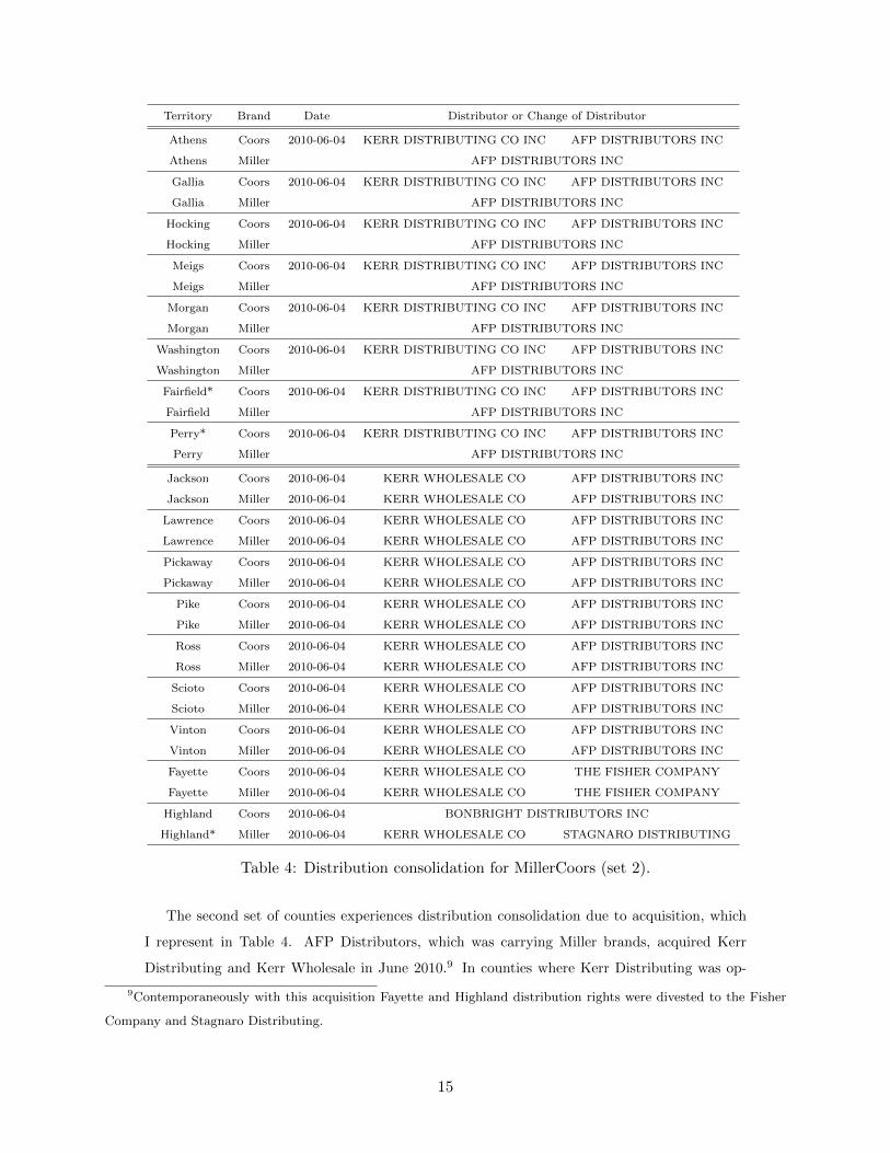
Table 4: Distribution consolidation for MillerCoors (set 2).
The second set of counties experiences distribution consolidation due to acquisition, which
I represent in Table 4. AFP Distributors, which was carrying Miller brands, acquired Kerr
Distributing and Kerr Wholesale in June 2010.9 In counties where Kerr Distributing was op-
9Contemporaneously with this acquisition Fayette and Highland distribution rights were divested to the Fisher
Company and Stagnaro Distributing.
15
erating, this acquisition led to consolidation of Miller and Coors brands in the hands of AFP
Distributors. In counties where Kerr Wholesale was operating, Miller and Coors were already
consolidated, so the change of ownership from Kerr Wholesale to AFP Distributors did not
affect the distribution consolidation status. Thus, counties of Kerr Distributing will serve as
treatment counties for this event, which I will call event 2 in the rest of the paper. Counties
of Kerr Wholesale will serve as control counties, along with many other counties where the
distribution consolidation status did not change.
Again, there are county-brand combinations divided into smaller territories (starred). With-
out documenting here which distributors carry the brands in parts of these counties, I sim-
ply state that the existence of county sub-division does not allow for clean data construction.
Similarly to analogous situation with event 1, I cannot tell whether distribution consolidation
happened or not in the upstream of the specific stores I observe. Thus, such counties (Fairfield,
Perry, Highland) are dropped from the analysis.
Finally, it turns out that all of the final distributors in the treatment counties also carried
Heineken and Modelo brands at the time when consolidation of MillerCoors distribution was
taking place. This means that not only Miller and Coors brands were consolidated in the hands
of one distributor, but also a brand that was transferred (Miller or Coors) was newly co-carried
with Heineken and Modelo. So, these brands should also be considered as “consolidated” brands,
along with Miller and Coors.
I explain my empirical strategy in more detail in section 5, but before that it is useful to
describe the uniform pricing which the chains employ across the state of Ohio.
4 Evidence on Uniform Pricing
As will be clear from the graphs below, the degree to which chains participate in uniform pricing
is quite high. However, it is not perfect in the sense that there are stores which deviate from
the median price in almost any week for a wide range of products. To illustrate these two points
I construct the following statistics. For each chain c, week t and product j, build a median
normalized10 price pmedjct across the stores s of chain c, and build the 10% and 90% empirical
percentiles of normalized prices.
10Where normalization is, as before, in terms of price for an equivalent of 144-oz. product volume.
16
2009010120090501
2009090120100101
2010050120100901
2011010120110501
2011090120120101
10.00
10.25
10.50
10.75
11.00
11.25
11.50
11.75
12.00COORS LIGHT 6-packMILLER LITE 6-pack
2009010120090501
2009090120100101
2010050120100901
2011010120110501
2011090120120101
8.75
9.00
9.25
9.50
9.75
10.00
10.25
10.50COORS LIGHT 12-packMILLER LITE 12-pack
2009010120090501
2009090120100101
2010050120100901
2011010120110501
2011090120120101
8.0
8.2
8.4
8.6
8.8
9.0
9.2
9.4COOR LIGHT 24-packMILLER LITE 24-pack
2009010120090501
2009090120100101
2010050120100901
2011010120110501
2011090120120101
10.5
11.0
11.5
12.0
COORS LIGHT 6-packMILLER LITE 6-pack
2009010120090501
2009090120100101
2010050120100901
2011010120110501
2011090120120101
9.00
9.25
9.50
9.75
10.00
10.25
10.50
COORS LIGHT 12-packMILLER LITE 12-pack
2009010120090501
2009090120100101
2010050120100901
2011010120110501
2011090120120101
8.0
8.2
8.4
8.6
8.8
9.0
9.2
9.4
9.6 COORS LIGHT 24-packMILLER LITE 24-pack
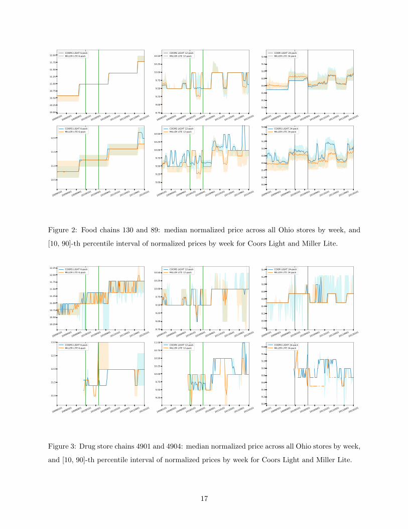
Figure 2: Food chains 130 and 89: median normalized price across all Ohio stores by week, and
[10, 90]-th percentile interval of normalized prices by week for Coors Light and Miller Lite.
2009010120090501
2009090120100101
2010050120100901
2011010120110501
2011090120120101
10.25
10.50
10.75
11.00
11.25
11.50
11.75
12.00
12.25 COORS LIGHT 6-packMILLER LITE 6-pack
2009010120090501
2009090120100101
2010050120100901
2011010120110501
2011090120120101
8.75
9.00
9.25
9.50
9.75
10.00
10.25
10.50COORS LIGHT 12-packMILLER LITE 12-pack
2009010120090501
2009090120100101
2010050120100901
2011010120110501
2011090120120101
7.8
8.0
8.2
8.4
8.6
8.8
9.0
9.2
9.4 COOR LIGHT 24-packMILLER LITE 24-pack
2009010120090501
2009090120100101
2010050120100901
2011010120110501
2011090120120101
11.0
11.5
12.0
12.5
13.0COORS LIGHT 6-packMILLER LITE 6-pack
2009010120090501
2009090120100101
2010050120100901
2011010120110501
2011090120120101
9.25
9.50
9.75
10.00
10.25
10.50
10.75
11.00COORS LIGHT 12-packMILLER LITE 12-pack
2009010120090501
2009090120100101
2010050120100901
2011010120110501
2011090120120101
8.0
8.2
8.4
8.6
8.8
9.0
9.2
9.4
9.6COORS LIGHT 24-packMILLER LITE 24-pack
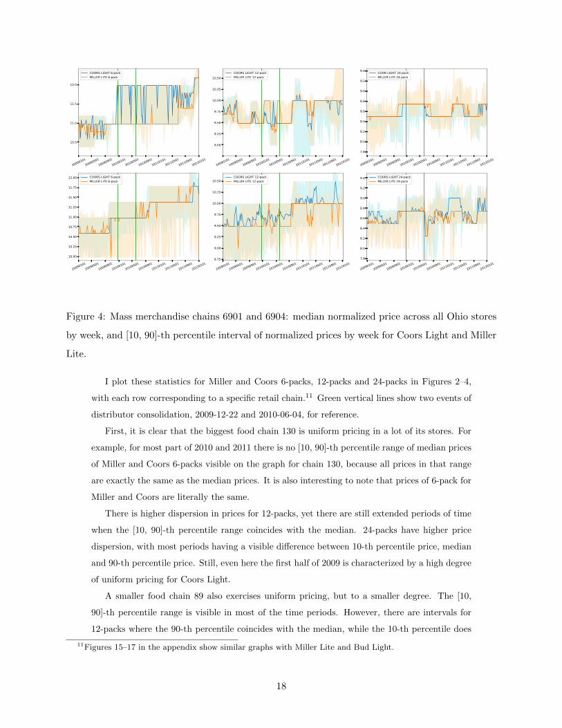
Figure 3: Drug store chains 4901 and 4904: median normalized price across all Ohio stores by week,
and [10, 90]-th percentile interval of normalized prices by week for Coors Light and Miller Lite.
17
2009010120090501
2009090120100101
2010050120100901
2011010120110501
2011090120120101
10.5
11.0
11.5
12.0
COORS LIGHT 6-packMILLER LITE 6-pack
2009010120090501
2009090120100101
2010050120100901
2011010120110501
2011090120120101
9.00
9.25
9.50
9.75
10.00
10.25
10.50COORS LIGHT 12-packMILLER LITE 12-pack
2009010120090501
2009090120100101
2010050120100901
2011010120110501
2011090120120101
7.8
8.0
8.2
8.4
8.6
8.8
9.0
9.2
9.4 COOR LIGHT 24-packMILLER LITE 24-pack
2009010120090501
2009090120100101
2010050120100901
2011010120110501
2011090120120101
10.00
10.25
10.50
10.75
11.00
11.25
11.50
11.75
12.00 COORS LIGHT 6-packMILLER LITE 6-pack
2009010120090501
2009090120100101
2010050120100901
2011010120110501
2011090120120101
8.75
9.00
9.25
9.50
9.75
10.00
10.25
10.50COORS LIGHT 12-packMILLER LITE 12-pack
2009010120090501
2009090120100101
2010050120100901
2011010120110501
2011090120120101
7.8
8.0
8.2
8.4
8.6
8.8
9.0
9.2
9.4 COORS LIGHT 24-packMILLER LITE 24-pack
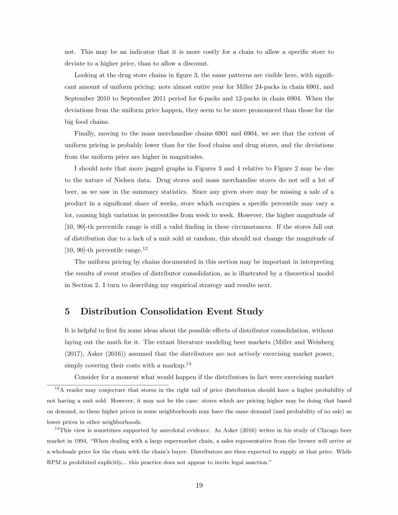
Figure 4: Mass merchandise chains 6901 and 6904: median normalized price across all Ohio stores
by week, and [10, 90]-th percentile interval of normalized prices by week for Coors Light and Miller
Lite.
I plot these statistics for Miller and Coors 6-packs, 12-packs and 24-packs in Figures 2–4,
with each row corresponding to a specific retail chain.11 Green vertical lines show two events of
distributor consolidation, 2009-12-22 and 2010-06-04, for reference.
First, it is clear that the biggest food chain 130 is uniform pricing in a lot of its stores. For
example, for most part of 2010 and 2011 there is no [10, 90]-th percentile range of median prices
of Miller and Coors 6-packs visible on the graph for chain 130, because all prices in that range
are exactly the same as the median prices. It is also interesting to note that prices of 6-pack for
Miller and Coors are literally the same.
There is higher dispersion in prices for 12-packs, yet there are still extended periods of time
when the [10, 90]-th percentile range coincides with the median. 24-packs have higher price
dispersion, with most periods having a visible difference between 10-th percentile price, median
and 90-th percentile price. Still, even here the first half of 2009 is characterized by a high degree
of uniform pricing for Coors Light.
A smaller food chain 89 also exercises uniform pricing, but to a smaller degree. The [10,
90]-th percentile range is visible in most of the time periods. However, there are intervals for
12-packs where the 90-th percentile coincides with the median, while the 10-th percentile does
11Figures 15–17 in the appendix show similar graphs with Miller Lite and Bud Light.
18
not. This may be an indicator that it is more costly for a chain to allow a specific store to
deviate to a higher price, than to allow a discount.
Looking at the drug store chains in figure 3, the same patterns are visible here, with signifi-
cant amount of uniform pricing: note almost entire year for Miller 24-packs in chain 6901, and
September 2010 to September 2011 period for 6-packs and 12-packs in chain 6904. When the
deviations from the uniform price happen, they seem to be more pronounced than those for the
big food chains.
Finally, moving to the mass merchandise chains 6901 and 6904, we see that the extent of
uniform pricing is probably lower than for the food chains and drug stores, and the deviations
from the uniform price are higher in magnitudes.
I should note that more jagged graphs in Figures 3 and 4 relative to Figure 2 may be due
to the nature of Nielsen data. Drug stores and mass merchandise stores do not sell a lot of
beer, as we saw in the summary statistics. Since any given store may be missing a sale of a
product in a significant share of weeks, store which occupies a specific percentile may vary a
lot, causing high variation in percentiles from week to week. However, the higher magnitude of
[10, 90]-th percentile range is still a valid finding in these circumstances. If the stores fall out
of distribution due to a lack of a unit sold at random, this should not change the magnitude of
[10, 90]-th percentile range.12
The uniform pricing by chains documented in this section may be important in interpreting
the results of event studies of distributor consolidation, as is illustrated by a theoretical model
in Section 2. I turn to describing my empirical strategy and results next.
5 Distribution Consolidation Event Study
It is helpful to first fix some ideas about the possible effects of distributor consolidation, without
laying out the math for it. The extant literature modeling beer markets (Miller and Weinberg
(2017), Asker (2016)) assumed that the distributors are not actively exercising market power,
simply covering their costs with a markup.13
Consider for a moment what would happen if the distributors in fact were exercising market
12A reader may conjecture that stores in the right tail of price distribution should have a higher probability of
not having a unit sold. However, it may not be the case: stores which are pricing higher may be doing that based
on demand, so these higher prices in some neighborhoods may have the same demand (and probability of no sale) as
lower prices in other neighborhoods.13This view is sometimes supported by anecdotal evidence. As Asker (2016) writes in his study of Chicago beer
market in 1994, “When dealing with a large supermarket chain, a sales representative from the brewer will arrive at
a wholesale price for the chain with the chain’s buyer. Distributors are then expected to supply at that price. While
RPM is prohibited explicitly... this practice does not appear to invite legal sanction.”
19
power. Consolidation of distribution, such as moving Miller brand to the same distributor who is
carrying Coors, Heineken and Modelo, would create the same incentives for the distributor as in
a usual horizontal merger. The distributor would be able to internalize the effect of raising Miller
prices on the demand for Coors, Heinieken and Modelo, and the other way around. This would
create upward pricing pressure for these brands. A distributor of a different, non-consolidated
brand, like ABI, will raise its prices in turn, following the usual logic of prices being strategic
complements in Nash-Bertrand price competition. However, this price increase would not be as
big as the price increase of consolidated brands, because ABI does not have the additional effect
of internalizing the pricing externality.
This description calls for a difference-in-difference approach to testing if distributors actively
exercise market power. If they do, following distributor consolidation, price increase of the
consolidated brands (Miller, Coors, Heineken, Modelo), should be higher than price change of
the brands not consolidated (ABI).
There is also a concern that contemporaneously with distributor consolidation there may be
some differential changes to the marginal costs of brands involved, which may contaminate the
results. For example, a decrease in marginal costs for only ABI would decrease its prices relative
to the brands involved in distribution consolidation, and give a false impression of the significant
effect of distributor marker power.14 In order to control for this, it is better to compare the
price changes in the counties that experienced the distributor consolidation to price changes in
counties which did not.15
The considerations above leads me to the following triple difference-in-difference empirical
specification:
log pjs(c)t(m) = γ1Itreatc + γ2Ipostt + γ3Itreatc · Ipostt +
+ γ4Itreatc · Iconsj + γ5Ipostt · Iconsj + γ6Itreatc · Ipostt · Iconsj +
+ αjc + βm + εjst
(1)
where indices are j for product, s for store, c for county, t for week, and m for month; the
observation level is product-week-store.
Price is regressed on the indicator of treatment Itreatc — the counties which experienced
distributor consolidation, indicator of post consolidation event Ipostt , their interaction, and in-
teractions of each of these three variables with the indicator of brands directly participating
in distributor consolidation Iconsj . The regression also includes chain-product fixed effects αjc
to control for the average price that a chain sets for a product, and month fixed effects βm to
14A contemporaneous state-wide change in the pricing policy of one of the manufacturers, like a price slash for a
state-wide sale of inventories by ABI, would be problematic in the same way.15Regardless of whether they were or were not consolidated in the first place. What is essential is that they do
not have a change of distribution event in the studied period.
20
control for seasonality in beer pricing. I use the entire period of 2009–2011 in the regressions
to be able to capture these seasonality effects from at least three years of data.16 I use robust
standard errors, clustered at the product level: graphical representation of prices in the previous
section indicates that prices of a given product may have common shocks across different chains.
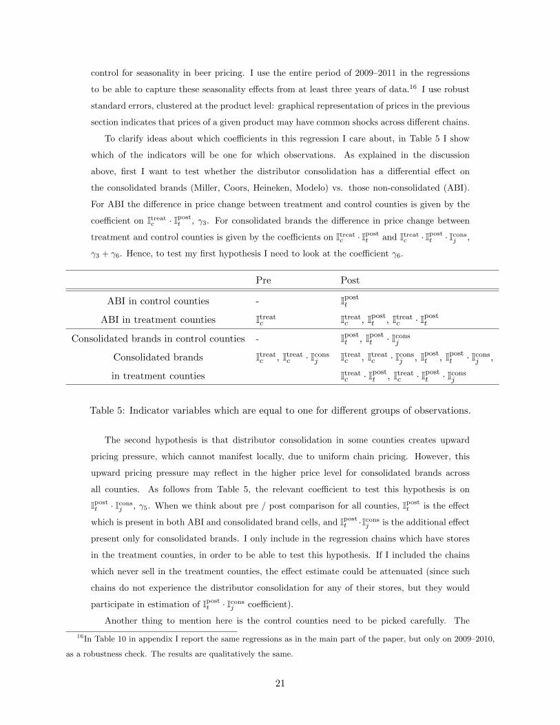
To clarify ideas about which coefficients in this regression I care about, in Table 5 I show
which of the indicators will be one for which observations. As explained in the discussion
above, first I want to test whether the distributor consolidation has a differential effect on
the consolidated brands (Miller, Coors, Heineken, Modelo) vs. those non-consolidated (ABI).
For ABI the difference in price change between treatment and control counties is given by the
coefficient on Itreatc · Ipostt , γ3. For consolidated brands the difference in price change between
treatment and control counties is given by the coefficients on Itreatc · Ipostt and Itreatc · Ipostt · Iconsj ,
γ3 + γ6. Hence, to test my first hypothesis I need to look at the coefficient γ6.
Pre Post
ABI in control counties - Ipostt
ABI in treatment counties Itreatc Itreat
c , Ipostt , Itreat
c · Ipostt
Consolidated brands in control counties - Ipostt , Ipost
t · Iconsj
Consolidated brands Itreatc , Itreat
c · Iconsj Itreat
c , Itreatc · Icons
j , Ipostt , Ipost
t · Iconsj ,
in treatment counties Itreatc · Ipost
t , Itreatc · Ipost
t · Iconsj
Table 5: Indicator variables which are equal to one for different groups of observations.
The second hypothesis is that distributor consolidation in some counties creates upward
pricing pressure, which cannot manifest locally, due to uniform chain pricing. However, this
upward pricing pressure may reflect in the higher price level for consolidated brands across
all counties. As follows from Table 5, the relevant coefficient to test this hypothesis is on
Ipostt · Iconsj , γ5. When we think about pre / post comparison for all counties, Ipostt is the effect
which is present in both ABI and consolidated brand cells, and Ipostt ·Iconsj is the additional effect
present only for consolidated brands. I only include in the regression chains which have stores
in the treatment counties, in order to be able to test this hypothesis. If I included the chains
which never sell in the treatment counties, the effect estimate could be attenuated (since such
chains do not experience the distributor consolidation for any of their stores, but they would
participate in estimation of Ipostt · Iconsj coefficient).
Another thing to mention here is the control counties need to be picked carefully. The
16In Table 10 in appendix I report the same regressions as in the main part of the paper, but only on 2009–2010,
as a robustness check. The results are qualitatively the same.
21
counties which are participating or ambiguous in distributor consolidation for event 2 cannot be
used as control counties for event 1.17 For example, if there is a distribution consolidation effect,
such counties of event 2, if included in the regression for event 1 as control, will experience it in
the post period in control group, and this will bias the estimate of γ6 down. Consistently with
this logic and the description of the data in Tables 3 and 4 counties Athens, Gallia, Hocking,
Meigs, Morgan, Washington (treatment of event 2) are excluded from the regression for event 1.
Counties Darke and Shelby (treatment of event 1) are excluded from the regression for event 2.
Counties Champaign, Mercer, Auglaize, Logan, Fairfield, Perry and Highland (those for which
I cannot tell apart the stores where distribution consolidation happened vs. not) are excluded
from both regressions.
5.1 Contemporaneous effect of distributor consolidation
Table 6 reports the results of empirical specification 1, in column 1 for event 1 around December
2009, and in column 2 for event 2 around June 2010. First, it is useful to note that the prices
of both consolidated and non-consolidated brands are statistically the same in treatment and
control counties before distribution consolidation: both coefficients on Itreatc and Itreatc · Iconsj are
close to 0 and insignificant.18
Turning to the coefficient of interest on the interaction Itreatc ·Ipostt ·Iconsj , we see that it is close
to zero and not statistically significant. The point estimates of the effect of distribution con-
solidation effect on prices are −0.36% and 0.28% respectively. I should note, however, that my
standard errors are comparable to the point estimates. For event 1, the 95% confidence interval
of the distribution consolidation effect is [−1.21%, 0.49%], and for event 2 it is [−0.10%, 0.65%].
Thus, the largest positive effect I cannot reject is 0.65%. Overall I find these results indicative of
no economically important contemporaneous effect of distributor consolidation on consolidated
brands in treated counties.
Of course, this finding may not be very surprising, given the evidence of chain uniform
pricing I showed in section 4. If the store managers are constrained by the chain pricing policy,
they may not increase local prices even if the distributor in their area raises the wholesale prices
post-consolidation. This idea justifies the second test which I consider. The higher pricing
pressure by the consolidated distributor may reflect not in higher local prices, but rather in
higher prices across the entire state of Ohio. As discussed above, the coefficient on Ipostt · Iconsj
17and vice versa18I drop Michelob brands in all regressions, and only keep Budweiser and Bud Light for ABI. This is driven by
the fact that Michelob brands were actually priced differently in the treatment and control counties pre-distribution
change, as opposed to the other brands included in the regression. This potentially indicated that Michelob brands,
as more niche, are not very suitable as a control group.
22

Chains present Chains not present
in treatment counties in treatment counties
(1) (2) (3) (4)
Event 1 Event 2 Event 1 Event 2
log pjs(c)t(m)
Itreatc -0.00147 -0.000564
(0.00175) (0.00165)
Ipostt 0.0368*** 0.0384*** 0.0636*** 0.0529***
(0.00584) (0.00630) (0.0136) (0.0110)
Itreatc · Ipost
t 0.00495 -0.000247
(0.00356) (0.000822)
Itreatc · Icons
j 0.000858 -0.00406
(0.00302) (0.00262)
Ipostt · Icons
j -0.0139* -0.0166* -0.0400** -0.0303**
(0.00759) (0.00849) (0.0182) (0.0142)
Itreatc · Ipost
t · Iconsj -0.00357 0.00275
(0.00421) (0.00188)
Product-chain FE X X X X
Month FE X X X X
Product-clustered SE X X X X
Observations 1,001,064 1,574,144 46,948 46,948
R2 0.993 0.993 0.949 0.948
Table 6: Estimates of log price regression on indicators of treatment counties, post-treatment,
consolidated brands, and their interactions, 2009–2011 sample. Product-clustered standard errors
in parentheses.
23
tests this hypothesis.
The respective point estimates are −1.39% and −1.66%, significant at the 10% level. If
anything, prices changes of consolidated brands were lower than price changes of ABI.19
The idea that distributor consolidation may not only affect the stores in the distributor’s
territories, but the entire chain, allows for some additional evidence. There are chains in my
data which never sold in the territories treated by the distributor change. These are the smaller
food chains 295 and 9104, mass merchandise chain 6914 and convenience store chain 8199, selling
a combined 1.5% of the selected beer brands in Nielsen data.
For these chains I run a simpler difference-in-difference specification:
log pjs(c)t(m) = γ2Ipostt + γ5Ipostt · Iconsj +
+ αjc + βm + εjst
(2)
This regression allows me to see price increases of ABI, and price increases of other brands
post-distribution change for the chains which should not have been affected by the distribution
change at all. The results are reported in columns 3 and 4 of Table 6. For some reason ABI
prices increased more at these chains than chains from regressions 1–2 (compare 6.36% increase
to 3.68% for event 1, and 5.29% increase to 3.84% for event 2). However, price increases of
other brands were the same. Summing up γ2 + γ5, for event 1 we have 2.29% price increase of
consolidated brands for the chains present in counties with newly consolidated distributors, and
2.36% increase for the chains not present. For event 2, the estimated price increases are 2.18%
and 2.26%.
Interpretation of these findings is a little complicated by the differential effect of ABI. If
one believes that ABI is the correct control group when comparing column 1 to 3, and column
2 to 4, she would conclude the following. For chains which were not treated by distribution
consolidation, price changes of Miller, Coors, Heineken and Modelo brands have a bigger gap
with ABI price changes. Thus, the distributor consolidation must have had a positive effect on
prices at the chains to which consolidated distributors do sell.
However, my interpretation is that the differential price changes of ABI in these columns
indicate something idiosyncratic to ABI and the small chains which participate in regressions (3),
(4).20 To me close price changes of Miller, Coors, Heineken and Modelo in chains to which newly
consolidated distributors do and do not sell serve as additional evidence that contemporaneously
the distribution structure did not have an effect on the overall pricing of a chain.
19I should note that this finding could also be explained by different changes in marginal costs for ABI and
consolidated brands around the same point in time.20Note that this was not a problem for interpretation of results in columns 1 and 2 in solitary, since the additional
effect on ABI brands in treatment counties (Itreatc · Ipostt ) was not statistically significant.
24
5.2 Lagged effect of distributor consolidation
In this subsection I show, first, evidence of parallel trends before the consolidation event, and,
second, evidence of lagged effect for event 2.
To illustrate the validity of parallel trends assumption, the date of ‘placebo’ event is placed
in different parts of the timeline to show that there is no significant effect before the actual event
date. A reader would like to see that, when placed in the ‘placebo’ spots, the event dummy
interacted with relevant variables is not statistically significant. If these placebo tests turn out
to fail (showing a significant coefficient) before the actual event, this may indicate a potential
problem with identification: it would seem that there are some unobserved events which lead to
effects being different in treatment and control groups.
If a significant coefficient is found after the actual event, this indicates a lagged effect of the
distributor consolidation, which is another reason to do this exercise.
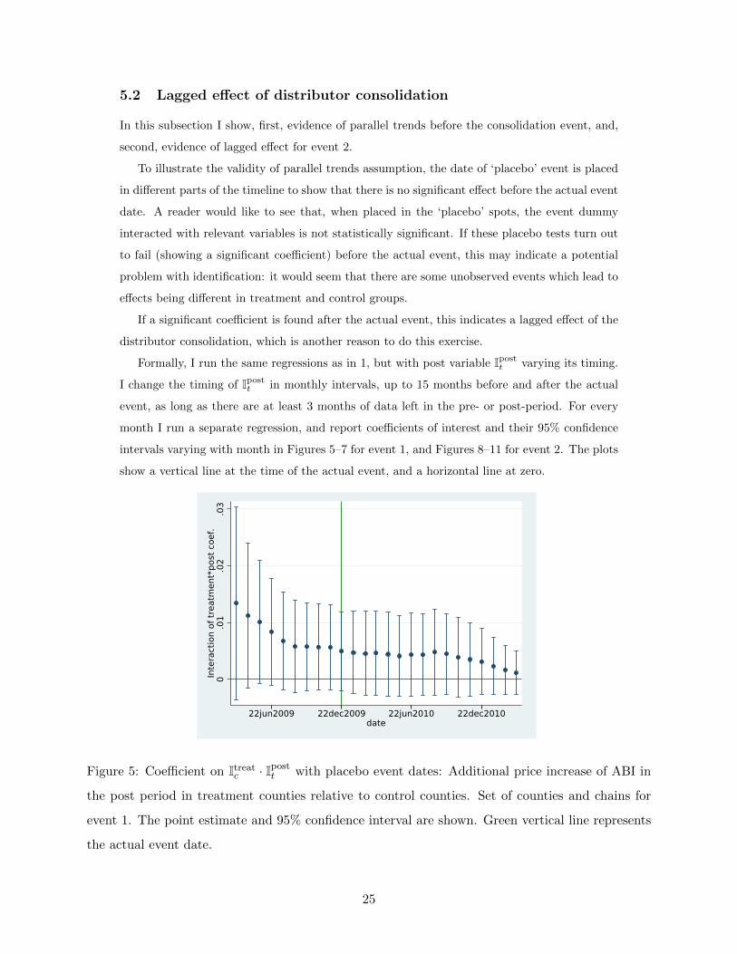
Formally, I run the same regressions as in 1, but with post variable Ipostt varying its timing.
I change the timing of Ipostt in monthly intervals, up to 15 months before and after the actual
event, as long as there are at least 3 months of data left in the pre- or post-period. For every
month I run a separate regression, and report coefficients of interest and their 95% confidence
intervals varying with month in Figures 5–7 for event 1, and Figures 8–11 for event 2. The plots
show a vertical line at the time of the actual event, and a horizontal line at zero.
0.0
1.0
2.0
3In
tera
ctio
n of
trea
tmen
t*po
st c
oef.
22jun2009 22dec2009 22jun2010 22dec2010date
Figure 5: Coefficient on Itreatc · Ipost
t with placebo event dates: Additional price increase of ABI in
the post period in treatment counties relative to control counties. Set of counties and chains for
event 1. The point estimate and 95% confidence interval are shown. Green vertical line represents
the actual event date.
25
I start the analysis with event 1, coefficient on Itreatc ·Ipostt , which is shown in Figure 5. Recall
from Table 5 that this is the additional price increase of ABI in the treatment counties relative
to control counties in the post period. It is useful to look at this coefficient to check if the
control group — ABI brands — is experiencing any differential price changes in treatment vs
control counties. We can see that all the coefficients for both pre-actual event and post-actual
event are not significantly different from zero. So, price increases of ABI are the same in control
and treatment counties, which is what we could expect, given that ABI brands are not directly
affected by distributor consolidation.21
-.04
-.03
-.02
-.01
0In
tera
ctio
n of
pos
t*co
nsol
idat
ed b
rand
s co
ef.
22jun2009 22dec2009 22jun2010 22dec2010date
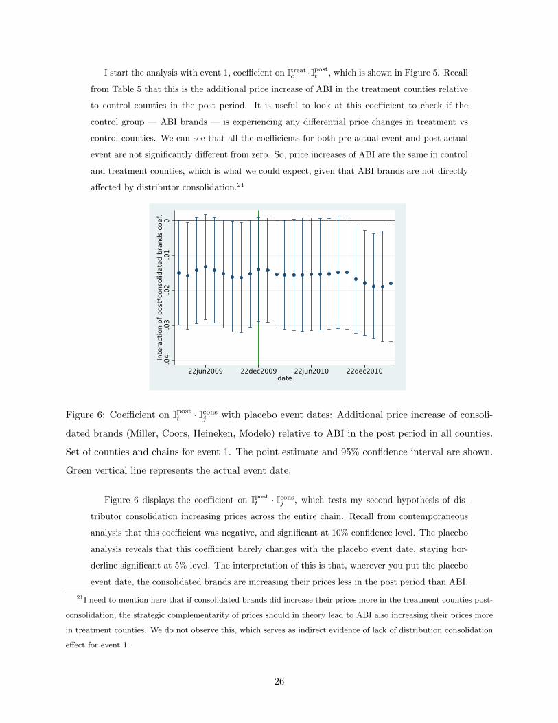
Figure 6: Coefficient on Ipostt · Icons
j with placebo event dates: Additional price increase of consoli-
dated brands (Miller, Coors, Heineken, Modelo) relative to ABI in the post period in all counties.
Set of counties and chains for event 1. The point estimate and 95% confidence interval are shown.
Green vertical line represents the actual event date.
Figure 6 displays the coefficient on Ipostt · Iconsj , which tests my second hypothesis of dis-
tributor consolidation increasing prices across the entire chain. Recall from contemporaneous
analysis that this coefficient was negative, and significant at 10% confidence level. The placebo
analysis reveals that this coefficient barely changes with the placebo event date, staying bor-
derline significant at 5% level. The interpretation of this is that, wherever you put the placebo
event date, the consolidated brands are increasing their prices less in the post period than ABI.
21I need to mention here that if consolidated brands did increase their prices more in the treatment counties post-
consolidation, the strategic complementarity of prices should in theory lead to ABI also increasing their prices more
in treatment counties. We do not observe this, which serves as indirect evidence of lack of distribution consolidation
effect for event 1.
26
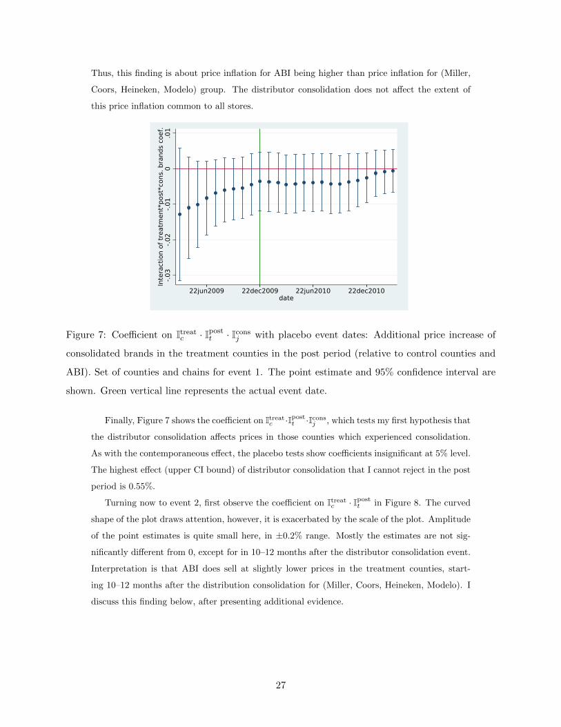
Thus, this finding is about price inflation for ABI being higher than price inflation for (Miller,
Coors, Heineken, Modelo) group. The distributor consolidation does not affect the extent of
this price inflation common to all stores.
-.03
-.02
-.01
0.0
1In
tera
ctio
n of
trea
tmen
t*po
st*c
ons.
bra
nds
coef
.
22jun2009 22dec2009 22jun2010 22dec2010date
Figure 7: Coefficient on Itreatc · Ipost
t · Iconsj with placebo event dates: Additional price increase of
consolidated brands in the treatment counties in the post period (relative to control counties and
ABI). Set of counties and chains for event 1. The point estimate and 95% confidence interval are
shown. Green vertical line represents the actual event date.
Finally, Figure 7 shows the coefficient on Itreatc ·Ipostt ·Iconsj , which tests my first hypothesis that
the distributor consolidation affects prices in those counties which experienced consolidation.
As with the contemporaneous effect, the placebo tests show coefficients insignificant at 5% level.
The highest effect (upper CI bound) of distributor consolidation that I cannot reject in the post
period is 0.55%.
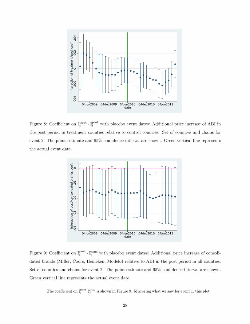
Turning now to event 2, first observe the coefficient on Itreatc · Ipostt in Figure 8. The curved
shape of the plot draws attention, however, it is exacerbated by the scale of the plot. Amplitude
of the point estimates is quite small here, in ±0.2% range. Mostly the estimates are not sig-
nificantly different from 0, except for in 10–12 months after the distributor consolidation event.
Interpretation is that ABI does sell at slightly lower prices in the treatment counties, start-
ing 10–12 months after the distribution consolidation for (Miller, Coors, Heineken, Modelo). I
discuss this finding below, after presenting additional evidence.
27
-.004
-.002
0.0
02.0
04In
tera
ctio
n of
trea
tmen
t*po
st c
oef.
04jun2009 04dec2009 04jun2010 04dec2010 04jun2011date
Figure 8: Coefficient on Itreatc · Ipost
t with placebo event dates: Additional price increase of ABI in
the post period in treatment counties relative to control counties. Set of counties and chains for
event 2. The point estimate and 95% confidence interval are shown. Green vertical line represents
the actual event date.
-.04
-.03
-.02
-.01
0In
tera
ctio
n of
pos
t*co
nsol
idat
ed b
rand
s co
ef.
04jun2009 04dec2009 04jun2010 04dec2010 04jun2011date
Figure 9: Coefficient on Ipostt · Icons
j with placebo event dates: Additional price increase of consoli-
dated brands (Miller, Coors, Heineken, Modelo) relative to ABI in the post period in all counties.
Set of counties and chains for event 2. The point estimate and 95% confidence interval are shown.
Green vertical line represents the actual event date.
The coefficient on Ipostt ·Iconsj is shown in Figure 9. Mirroring what we saw for event 1, this plot
28
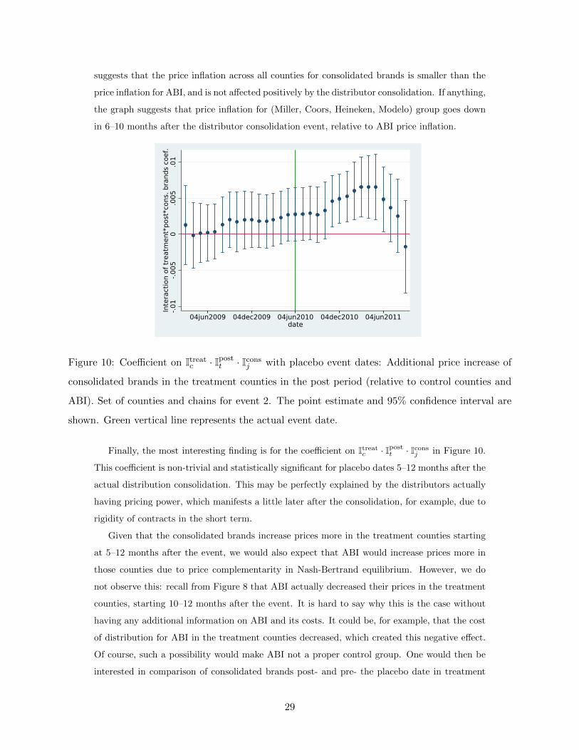
suggests that the price inflation across all counties for consolidated brands is smaller than the
price inflation for ABI, and is not affected positively by the distributor consolidation. If anything,
the graph suggests that price inflation for (Miller, Coors, Heineken, Modelo) group goes down
in 6–10 months after the distributor consolidation event, relative to ABI price inflation.
-.01
-.005
0.0
05.0
1In
tera
ctio
n of
trea
tmen
t*po
st*c
ons.
bra
nds
coef
.
04jun2009 04dec2009 04jun2010 04dec2010 04jun2011date
Figure 10: Coefficient on Itreatc · Ipost
t · Iconsj with placebo event dates: Additional price increase of
consolidated brands in the treatment counties in the post period (relative to control counties and
ABI). Set of counties and chains for event 2. The point estimate and 95% confidence interval are
shown. Green vertical line represents the actual event date.
Finally, the most interesting finding is for the coefficient on Itreatc · Ipostt · Iconsj in Figure 10.
This coefficient is non-trivial and statistically significant for placebo dates 5–12 months after the
actual distribution consolidation. This may be perfectly explained by the distributors actually
having pricing power, which manifests a little later after the consolidation, for example, due to
rigidity of contracts in the short term.
Given that the consolidated brands increase prices more in the treatment counties starting
at 5–12 months after the event, we would also expect that ABI would increase prices more in
those counties due to price complementarity in Nash-Bertrand equilibrium. However, we do
not observe this: recall from Figure 8 that ABI actually decreased their prices in the treatment
counties, starting 10–12 months after the event. It is hard to say why this is the case without
having any additional information on ABI and its costs. It could be, for example, that the cost
of distribution for ABI in the treatment counties decreased, which created this negative effect.
Of course, such a possibility would make ABI not a proper control group. One would then be
interested in comparison of consolidated brands post- and pre- the placebo date in treatment
29
and control counties, without ABI as a reference point, that is, not just the coefficient on
Itreatc · Ipostt · Iconsj , but the sum of Itreatc · Ipostt and Itreatc · Ipostt · Iconsj (see Table 5).
-.01
-.005
0.0
05.0
1Su
m o
f tre
atm
ent*
post
& tr
eatm
ent*
post
*con
s. c
oef.
04jun2009 04dec2009 04jun2010 04dec2010 04jun2011date
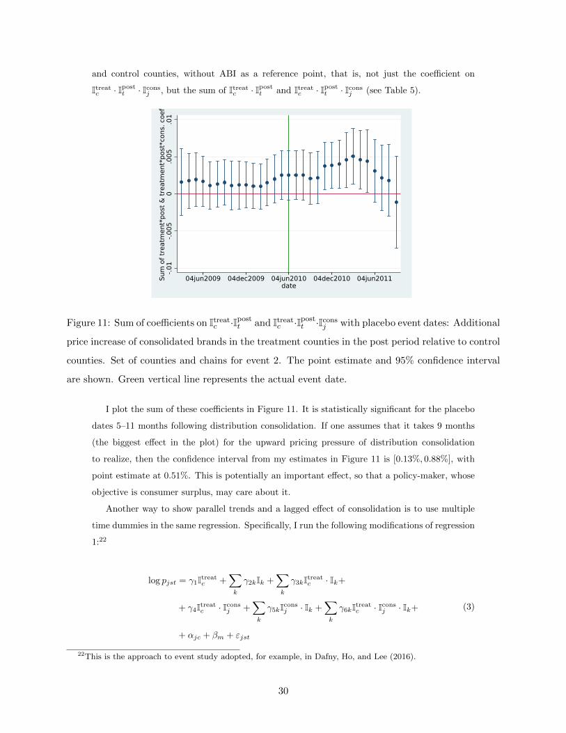
Figure 11: Sum of coefficients on Itreatc ·Ipost
t and Itreatc ·Ipost
t ·Iconsj with placebo event dates: Additional
price increase of consolidated brands in the treatment counties in the post period relative to control
counties. Set of counties and chains for event 2. The point estimate and 95% confidence interval
are shown. Green vertical line represents the actual event date.
I plot the sum of these coefficients in Figure 11. It is statistically significant for the placebo
dates 5–11 months following distribution consolidation. If one assumes that it takes 9 months
(the biggest effect in the plot) for the upward pricing pressure of distribution consolidation
to realize, then the confidence interval from my estimates in Figure 11 is [0.13%, 0.88%], with
point estimate at 0.51%. This is potentially an important effect, so that a policy-maker, whose
objective is consumer surplus, may care about it.
Another way to show parallel trends and a lagged effect of consolidation is to use multiple
time dummies in the same regression. Specifically, I run the following modifications of regression
1:22
log pjst = γ1Itreatc +∑k
γ2kIk +∑k
γ3kItreatc · Ik+
+ γ4Itreatc · Iconsj +∑k
γ5kIconsj · Ik +∑k
γ6kItreatc · Iconsj · Ik+
+ αjc + βm + εjst
(3)
22This is the approach to event study adopted, for example, in Dafny, Ho, and Lee (2016).
30
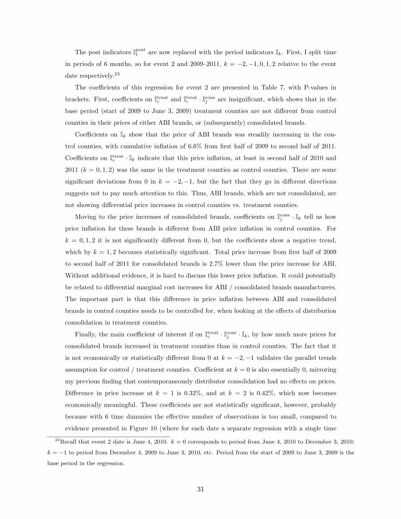
The post indicators Ipostt are now replaced with the period indicators Ik. First, I split time
in periods of 6 months, so for event 2 and 2009–2011, k = −2,−1, 0, 1, 2 relative to the event
date respectively.23
The coefficients of this regression for event 2 are presented in Table 7, with P-values in
brackets. First, coefficients on Itreatc and Itreatc · Iconsj are insignificant, which shows that in the
base period (start of 2009 to June 3, 2009) treatment counties are not different from control
counties in their prices of either ABI brands, or (subsequently) consolidated brands.
Coefficients on Ik show that the price of ABI brands was steadily increasing in the con-
trol counties, with cumulative inflation of 6.6% from first half of 2009 to second half of 2011.
Coefficients on Itreatc · Ik indicate that this price inflation, at least in second half of 2010 and
2011 (k = 0, 1, 2) was the same in the treatment counties as control counties. There are some
significant deviations from 0 in k = −2,−1, but the fact that they go in different directions
suggests not to pay much attention to this. Thus, ABI brands, which are not consolidated, are
not showing differential price increases in control counties vs. treatment counties.
Moving to the price increases of consolidated brands, coefficients on Iconsj · Ik tell us how
price inflation for these brands is different from ABI price inflation in control counties. For
k = 0, 1, 2 it is not significantly different from 0, but the coefficients show a negative trend,
which by k = 1, 2 becomes statistically significant. Total price increase from first half of 2009
to second half of 2011 for consolidated brands is 2.7% lower than the price increase for ABI.
Without additional evidence, it is hard to discuss this lower price inflation. It could potentially
be related to differential marginal cost increases for ABI / consolidated brands manufacturers.
The important part is that this difference in price inflation between ABI and consolidated
brands in control counties needs to be controlled for, when looking at the effects of distribution
consolidation in treatment counties.
Finally, the main coefficient of interest if on Itreatc · Iconsj · Ik, by how much more prices for
consolidated brands increased in treatment counties than in control counties. The fact that it
is not economically or statistically different from 0 at k = −2,−1 validates the parallel trends
assumption for control / treatment counties. Coefficient at k = 0 is also essentially 0, mirroring
my previous finding that contemporaneously distributor consolidation had no effects on prices.
Difference in price increase at k = 1 is 0.32%, and at k = 2 is 0.42%, which now becomes
economically meaningful. These coefficients are not statistically significant, however, probably
because with 6 time dummies the effective number of observations is too small, compared to
evidence presented in Figure 10 (where for each date a separate regression with a single time
23Recall that event 2 date is June 4, 2010. k = 0 corresponds to period from June 4, 2010 to December 3, 2010;
k = −1 to period from December 4, 2009 to June 3, 2010, etc. Period from the start of 2009 to June 3, 2009 is the
base period in the regression.
31
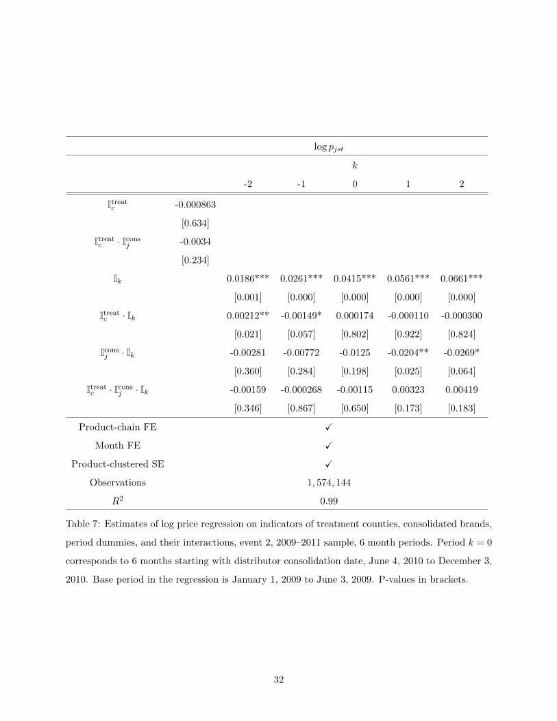
log pjst
k
-2 -1 0 1 2
Itreatc -0.000863
[0.634]
Itreatc · Icons
j -0.0034
[0.234]
Ik 0.0186*** 0.0261*** 0.0415*** 0.0561*** 0.0661***
[0.001] [0.000] [0.000] [0.000] [0.000]
Itreatc · Ik 0.00212** -0.00149* 0.000174 -0.000110 -0.000300
[0.021] [0.057] [0.802] [0.922] [0.824]
Iconsj · Ik -0.00281 -0.00772 -0.0125 -0.0204** -0.0269*
[0.360] [0.284] [0.198] [0.025] [0.064]
Itreatc · Icons
j · Ik -0.00159 -0.000268 -0.00115 0.00323 0.00419
[0.346] [0.867] [0.650] [0.173] [0.183]
Product-chain FE X
Month FE X
Product-clustered SE X
Observations 1, 574, 144
R2 0.99
Table 7: Estimates of log price regression on indicators of treatment counties, consolidated brands,
period dummies, and their interactions, event 2, 2009–2011 sample, 6 month periods. Period k = 0
corresponds to 6 months starting with distributor consolidation date, June 4, 2010 to December 3,
2010. Base period in the regression is January 1, 2009 to June 3, 2009. P-values in brackets.
32
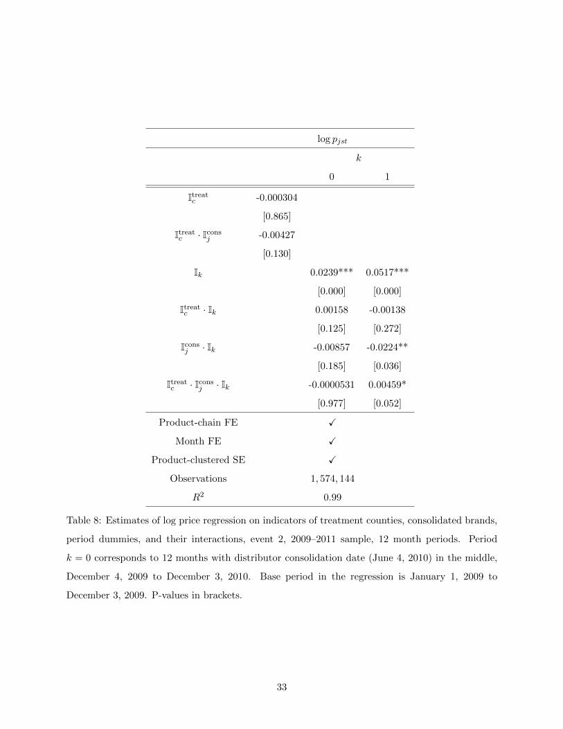
log pjst
k
0 1
Itreatc -0.000304
[0.865]
Itreatc · Icons
j -0.00427
[0.130]
Ik 0.0239*** 0.0517***
[0.000] [0.000]
Itreatc · Ik 0.00158 -0.00138
[0.125] [0.272]
Iconsj · Ik -0.00857 -0.0224**
[0.185] [0.036]
Itreatc · Icons
j · Ik -0.0000531 0.00459*
[0.977] [0.052]
Product-chain FE X
Month FE X
Product-clustered SE X
Observations 1, 574, 144
R2 0.99
Table 8: Estimates of log price regression on indicators of treatment counties, consolidated brands,
period dummies, and their interactions, event 2, 2009–2011 sample, 12 month periods. Period
k = 0 corresponds to 12 months with distributor consolidation date (June 4, 2010) in the middle,
December 4, 2009 to December 3, 2010. Base period in the regression is January 1, 2009 to
December 3, 2009. P-values in brackets.
33
dummy was estimated).
Thus, to provide evidence that the effects I am finding at k = 1, 2 are indeed statistically
significant, in Table 12 I present a similar regression, but with yearly time dummies instead of
half-yearly. Thus, the period contemporaneous with distributor consolidation, k = 0, is from
December 4, 2009 to December 3, 2010. Base period is January 1, 2009 to December 3, 2009.
In this regression qualitative evidence is the same as in Table 12, however, the coefficient on
Itreatc · Iconsj · Ik at k = 1 is now significant, with p-value of 0.052. Its magnitude is 0.46%, in
line with the previously shown effects in Figure 10 from regressions with a single time dummy.
Thus, the empirical evidence supports presence of price increases for the consolidated brands
following distributor consolidation in the treatment counties. It is somewhat unexpected that
prices of ABI are showing no differential price increases in the treatment counties vs. control
ones. The usual Nash equilibrium theory would suggest that ABI prices should rise through
unilateral response to prices of consolidated brands, but this is not observed in the coefficients
on Itreatc · Ik. A possible explanation to this is that ABI partition of distributors to territories is
different from the consolidated brands. Multiple counties which are treated for the consolidated
brands, belong to several distributors for ABI. Those distributors may have some internal rules
about pricing uniformly in their counties, and not reacting strategically to a price increase in a
subset of counties treated by Miller / Coors / Heineken / Modelo distribution consolidation.
Finally, I run similar regressions for event 1. They do not warrant a full discussion, since the
results are similar to the evidence shown in Figures 5–7, confirming that distributor consolidation
has no price effects for event 1. An interested reader may find estimates of these regressions in
Appendix C.
6 Discussion
First, in Section 4 I document that the chains exercise uniform pricing, with the biggest chains
having as many as 90% of stores setting the same price for a given brand in extended periods
of time. Hence, any discussion of distributor consolidation effects needs to be done through the
prism of this uniform pricing. Does distributor consolidation create upward pricing pressure? If
it does not, is the reason that the distributors do not wield any pricing power in this market,
or that UPP is constrained by the chain uniform pricing policies?
I attempt to shed some light on these questions with the empirical specifications in Section
5. The results reveal two important findings. One hypothesis is that distributor consolidation
in a set of territories may affect the overall prices of a chain present in those territories. I do not
find any empirical evidence for this hypothesis. Overall prices of consolidated brands increase
by less than prices of ABI, and this tendency does not change after the consolidation event.
34
I also show that the prices of consolidated brands change by the same amount for the chains
which have stores in the territories treated by distributor consolidations and the chains which
do not.
The other hypothesis, that the distributors may affect prices in the very counties where
they consolidate, finds mixed support. For event 1, this does not seem to be the case, either
contemporaneously with distribution consolidation, or in 15 months following it, although I
cannot statistically reject an effect as high as 0.55%. For event 2, however, I observe a significant
effect around 9 months following consolidation. The price increase for consolidated brands
in treatment counties is 0.51% higher than in control counties, with [0.13%, 0.88%] as 95%
confidence interval.
Why then does consolidation have an effect in case of event 2, but not event 1? Recall that
event 1 affects fewer counties than event 2 (See Tables 3 and 4). A retail chain may want to
set uniform prices in all its stores, but the cost of doing so may be higher when the prices are
sub-optimal in bigger share of stores. So, it may be that in the case of event 1 uniform pricing
incentive was strong enough to contain upward pricing pressure by the consolidated distributor,
whereas for event 2 it was not, and differential price increases were realized approximately 9
months after the event.
7 Conclusion
In this paper I investigate the importance of modeling vertical structure of the industry when
analyzing price effects of horizontal mergers at the distribution level. I build a stylized model,
in which uniform pricing by the retailers interacts with price setting by the distributors. I show
possibility of the existence of two types of equilibria. In one type a merger of distributors in
one county affects retail prices only in that county, and in another type it affects prices in all
counties. The former equilibrium exists when the incentive to price uniformly is weak, and the
latter exists when it is strong. Although not in my theoretical analysis, it may also be the case
that distribution structure, as assumed by the prior literature, does not matter for pricing.
Thus, empirically I test the hypothesis that distributors in the beer markets exercise market
power by increasing prices when they consolidate ownership of multiple brands. I use data
on two events of distributor consolidation which happened in 2009 and 2010 in Ohio following
the creation of MillerCoors joint venture. I find no empirical evidence that the consolidated
distributor’s upward pricing pressure manifests in higher prices in all counties. I also test if the
consolidated brands increase prices more in the very counties where distributors consolidated.
I find no contemporaneous effects, but a positive and significant effect around 9 months after
one of the consolidation events.
35
I conclude that the distributors are likely to have some pricing power, which may not reflect
in the final retail prices because of the retailers’ desire to price uniformly. The approach of
disregarding the distributors / modeling them as non-price setting, adopted in the previous
literature, may miss an important mechanism of price increases. Taking my point estimate at
face value, not thinking about distributor consolidation may attribute around 0.5% of price
increases to other sources.
Bringing a more structural approach to the task may be a useful next step. There is a
potential for a structural estimation in which distributors and retailers are modeled explicitly,
with the distributors having some pricing power, and retailers having an incentive for uniform
pricing. Applying a structural model to the data may reveal, for example, what monetary value
the retail chains put on pricing uniformly. I leave this avenue to future research.
References
Ashenfelter, O. C., D. S. Hosken, and M. C. Weinberg (2015): “Efficiencies brewed:
pricing and consolidation in the US beer industry,” The RAND Journal of Economics, 46,
328–361.
Asker, J. (2016): “Diagnosing foreclosure due to exclusive dealing,” The Journal of Industrial
Economics, 64, 375–410.
Bernheim, B. D. and M. D. Whinston (1985): “Common marketing agency as a device for
facilitating collusion,” The RAND Journal of Economics, 269–281.
Burgdorf, J. (2019): “Impact of mandated exclusive territories in the US brewing industry:
Evidence from scanner level data,” International Journal of Industrial Organization, 63, 376–
416.
Dafny, L., K. Ho, and R. S. Lee (2016): “The price effects of cross-market hospital mergers,”
Tech. rep., National Bureau of Economic Research.
DellaVigna, S. and M. Gentzkow (2017): “Uniform pricing in us retail chains,” Tech. rep.,
National Bureau of Economic Research.
Miller, N. H. and M. C. Weinberg (2017): “Understanding the price effects of the Miller-
Coors joint venture,” Econometrica, 85, 1763–1791.
Nevo, A. (2001): “Measuring market power in the ready-to-eat cereal industry,” Econometrica,
69, 307–342.
36
Sass, T. R. and D. S. Saurman (1996): “Efficiency effects of exclusive territories: Evidence
from the Indiana beer market,” Economic Inquiry, 34, 597–615.
37
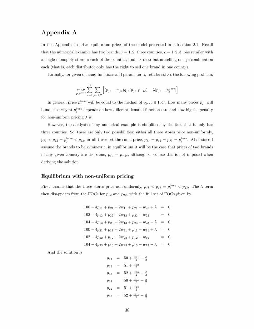
Appendix A
In this Appendix I derive equilibrium prices of the model presented in subsection 2.1. Recall
that the numerical example has two brands, j = 1, 2, three counties, c = 1, 2, 3, one retailer with
a single monopoly store in each of the counties, and six distributors selling one jc combination
each (that is, each distributor only has the right to sell one brand in one county).
Formally, for given demand functions and parameter λ, retailer solves the following problem:
maxp,pbase
C∑c=1
∑j=1,2
[(pjc − wjc)qjc(pjc, p−jc)− λ|pjc − pbasej |
]In general, price pbasej will be equal to the median of pjc, c ∈ 1, C. How many prices pjc will
bundle exactly at pbasej depends on how different demand functions are and how big the penalty
for non-uniform pricing λ is.
However, the analysis of my numerical example is simplified by the fact that it only has
three counties. So, there are only two possibilities: either all three stores price non-uniformly,
pj1 < pj2 = pbasej < pj2, or all three set the same price, pj1 = pj2 = pj3 = pbasej . Also, since I
assume the brands to be symmetric, in equilibrium it will be the case that prices of two brands
in any given country are the same, pjc = p−jc, although of course this is not imposed when
deriving the solution.
Equilibrium with non-uniform pricing
First assume that the three stores price non-uniformly, pj1 < pj2 = pbasej < pj2. The λ term
then disappears from the FOCs for p12 and p22, with the full set of FOCs given by
100− 4p11 + p21 + 2w11 + p21 − w21 + λ = 0
102− 4p12 + p22 + 2w12 + p22 − w22 = 0
104− 4p13 + p23 + 2w13 + p23 − w23 − λ = 0
100− 4p21 + p11 + 2w21 + p11 − w11 + λ = 0
102− 4p22 + p12 + 2w22 + p12 − w12 = 0
104− 4p23 + p13 + 2w23 + p13 − w13 − λ = 0
And the solution is
p11 = 50 + w11
2 + λ2
p12 = 51 + w12
2
p13 = 52 + w13
2 −λ2
p21 = 50 + w21
2 + λ2
p22 = 51 + w22
2
p23 = 52 + w23
2 −λ2
38
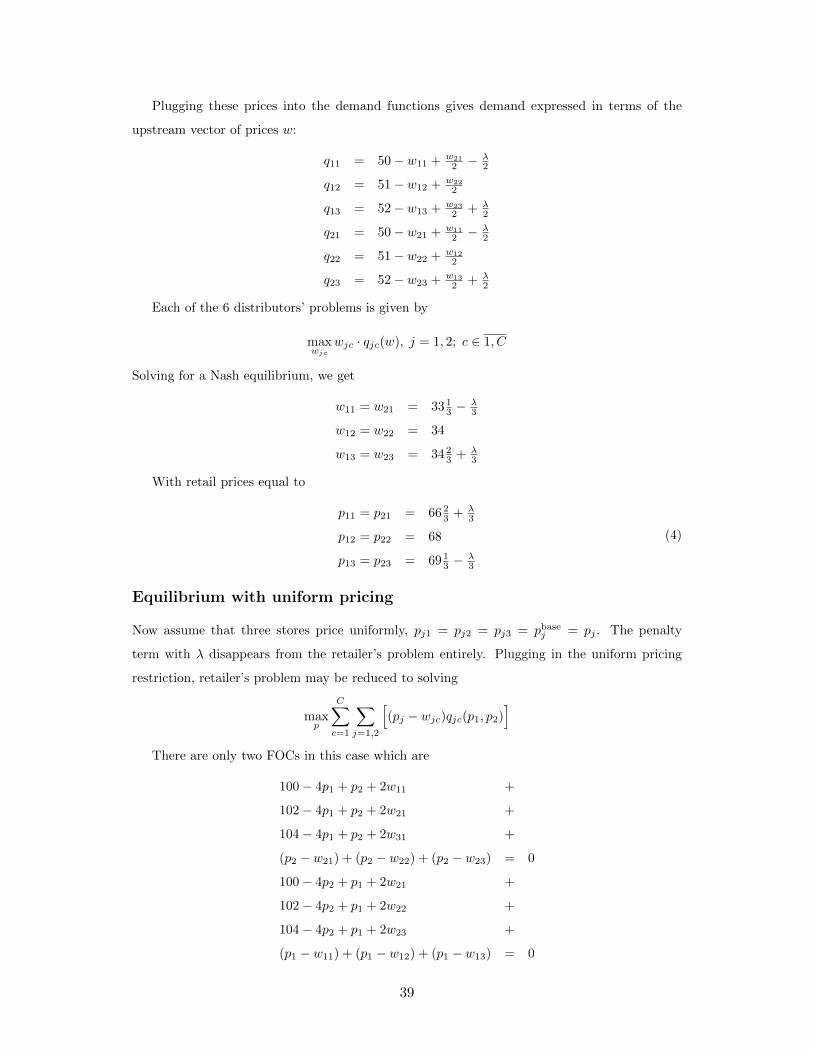
Plugging these prices into the demand functions gives demand expressed in terms of the
upstream vector of prices w:
q11 = 50− w11 + w21
2 −λ2
q12 = 51− w12 + w22
2
q13 = 52− w13 + w23
2 + λ2
q21 = 50− w21 + w11
2 −λ2
q22 = 51− w22 + w12
2
q23 = 52− w23 + w13
2 + λ2
Each of the 6 distributors’ problems is given by
maxwjc
wjc · qjc(w), j = 1, 2; c ∈ 1, C
Solving for a Nash equilibrium, we get
w11 = w21 = 33 13 −
λ3
w12 = w22 = 34
w13 = w23 = 34 23 + λ
3
With retail prices equal to
p11 = p21 = 66 23 + λ
3
p12 = p22 = 68
p13 = p23 = 69 13 −
λ3
(4)
Equilibrium with uniform pricing
Now assume that three stores price uniformly, pj1 = pj2 = pj3 = pbasej = pj . The penalty
term with λ disappears from the retailer’s problem entirely. Plugging in the uniform pricing
restriction, retailer’s problem may be reduced to solving
maxp
C∑c=1
∑j=1,2
[(pj − wjc)qjc(p1, p2)
]There are only two FOCs in this case which are
100− 4p1 + p2 + 2w11 +
102− 4p1 + p2 + 2w21 +
104− 4p1 + p2 + 2w31 +
(p2 − w21) + (p2 − w22) + (p2 − w23) = 0
100− 4p2 + p1 + 2w21 +
102− 4p2 + p1 + 2w22 +
104− 4p2 + p1 + 2w23 +
(p1 − w11) + (p1 − w12) + (p1 − w13) = 0
39
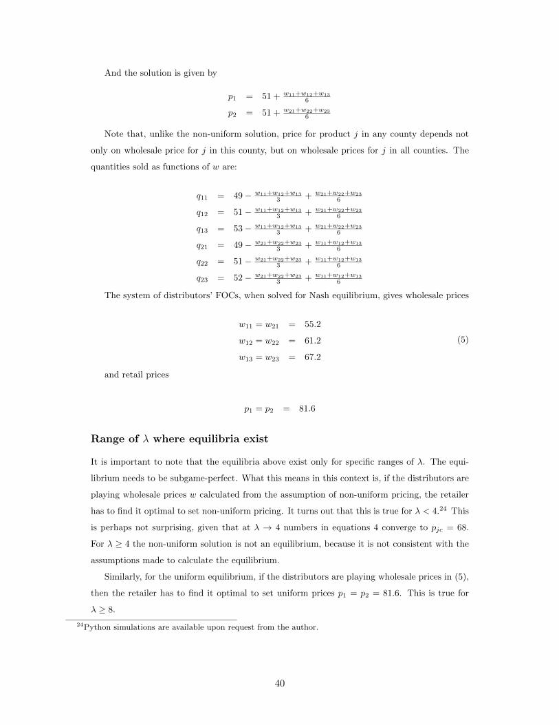
And the solution is given by
p1 = 51 + w11+w12+w13
6
p2 = 51 + w21+w22+w23
6
Note that, unlike the non-uniform solution, price for product j in any county depends not
only on wholesale price for j in this county, but on wholesale prices for j in all counties. The
quantities sold as functions of w are:
q11 = 49− w11+w12+w13
3 + w21+w22+w23
6
q12 = 51− w11+w12+w13
3 + w21+w22+w23
6
q13 = 53− w11+w12+w13
3 + w21+w22+w23
6
q21 = 49− w21+w22+w23
3 + w11+w12+w13
6
q22 = 51− w21+w22+w23
3 + w11+w12+w13
6
q23 = 52− w21+w22+w23
3 + w11+w12+w13
6
The system of distributors’ FOCs, when solved for Nash equilibrium, gives wholesale prices
w11 = w21 = 55.2
w12 = w22 = 61.2
w13 = w23 = 67.2
(5)
and retail prices
p1 = p2 = 81.6
Range of λ where equilibria exist
It is important to note that the equilibria above exist only for specific ranges of λ. The equi-
librium needs to be subgame-perfect. What this means in this context is, if the distributors are
playing wholesale prices w calculated from the assumption of non-uniform pricing, the retailer
has to find it optimal to set non-uniform pricing. It turns out that this is true for λ < 4.24 This
is perhaps not surprising, given that at λ → 4 numbers in equations 4 converge to pjc = 68.
For λ ≥ 4 the non-uniform solution is not an equilibrium, because it is not consistent with the
assumptions made to calculate the equilibrium.
Similarly, for the uniform equilibrium, if the distributors are playing wholesale prices in (5),
then the retailer has to find it optimal to set uniform prices p1 = p2 = 81.6. This is true for
λ ≥ 8.
24Python simulations are available upon request from the author.
40
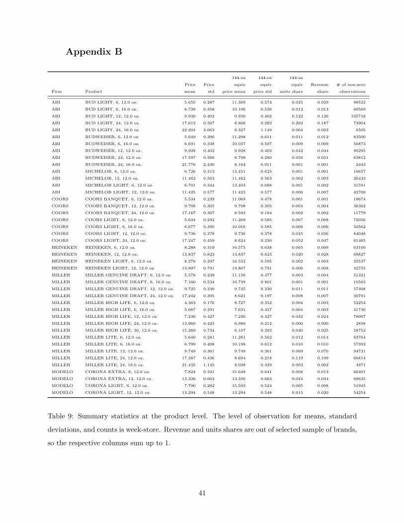
Appendix B
144-oz 144-oz 144-oz
Price Price equiv equiv equiv Revenue # of non-zero
Firm Product mean std price mean price std units share share observations
ABI BUD LIGHT, 6, 12.0 oz. 5.655 0.287 11.309 0.574 0.025 0.029 98522
ABI BUD LIGHT, 6, 16.0 oz. 6.738 0.358 10.106 0.536 0.012 0.013 60569
ABI BUD LIGHT, 12, 12.0 oz. 9.930 0.402 9.930 0.402 0.122 0.126 105718
ABI BUD LIGHT, 24, 12.0 oz. 17.612 0.567 8.806 0.283 0.202 0.187 73904
ABI BUD LIGHT, 24, 16.0 oz. 22.204 3.063 8.327 1.149 0.004 0.003 6505
ABI BUDWEISER, 6, 12.0 oz. 5.649 0.306 11.298 0.611 0.011 0.012 83500
ABI BUDWEISER, 6, 16.0 oz. 6.691 0.338 10.037 0.507 0.009 0.009 56873
ABI BUDWEISER, 12, 12.0 oz. 9.928 0.402 9.928 0.402 0.042 0.044 90295
ABI BUDWEISER, 24, 12.0 oz. 17.597 0.560 8.798 0.280 0.056 0.051 63812
ABI BUDWEISER, 24, 16.0 oz. 21.770 2.430 8.164 0.911 0.001 0.001 2443
ABI MICHELOB, 6, 12.0 oz. 6.726 0.313 13.451 0.625 0.001 0.001 16657
ABI MICHELOB, 12, 12.0 oz. 11.462 0.563 11.462 0.563 0.002 0.003 26433
ABI MICHELOB LIGHT, 6, 12.0 oz. 6.701 0.344 13.403 0.688 0.001 0.002 31591
ABI MICHELOB LIGHT, 12, 12.0 oz. 11.425 0.577 11.425 0.577 0.006 0.007 42700
COORS COORS BANQUET, 6, 12.0 oz. 5.534 0.239 11.069 0.478 0.001 0.001 18674
COORS COORS BANQUET, 12, 12.0 oz. 9.708 0.305 9.708 0.305 0.004 0.004 36362
COORS COORS BANQUET, 24, 12.0 oz. 17.187 0.367 8.593 0.184 0.002 0.002 11779
COORS COORS LIGHT, 6, 12.0 oz. 5.634 0.292 11.269 0.585 0.007 0.008 72056
COORS COORS LIGHT, 6, 16.0 oz. 6.677 0.390 10.016 0.585 0.006 0.006 50562
COORS COORS LIGHT, 12, 12.0 oz. 9.736 0.378 9.736 0.378 0.035 0.036 84048
COORS COORS LIGHT, 24, 12.0 oz. 17.247 0.459 8.624 0.230 0.052 0.047 61465
HEINEKEN HEINEKEN, 6, 12.0 oz. 8.288 0.319 16.575 0.638 0.005 0.009 63100
HEINEKEN HEINEKEN, 12, 12.0 oz. 13.837 0.823 13.837 0.823 0.020 0.028 68827
HEINEKEN HEINEKEN LIGHT, 6, 12.0 oz. 8.276 0.297 16.552 0.595 0.002 0.003 35537
HEINEKEN HEINEKEN LIGHT, 12, 12.0 oz. 13.807 0.791 13.807 0.791 0.006 0.008 42755
MILLER MILLER GENUINE DRAFT, 6, 12.0 oz. 5.578 0.239 11.156 0.477 0.003 0.004 51321
MILLER MILLER GENUINE DRAFT, 6, 16.0 oz. 7.160 0.534 10.739 0.801 0.001 0.001 10565
MILLER MILLER GENUINE DRAFT, 12, 12.0 oz. 9.725 0.330 9.725 0.330 0.011 0.011 57408
MILLER MILLER GENUINE DRAFT, 24, 12.0 oz. 17.242 0.395 8.621 0.197 0.008 0.007 30791
MILLER MILLER HIGH LIFE, 6, 12.0 oz. 4.363 0.176 8.727 0.352 0.004 0.003 52254
MILLER MILLER HIGH LIFE, 6, 16.0 oz. 5.087 0.291 7.631 0.437 0.004 0.003 41730
MILLER MILLER HIGH LIFE, 12, 12.0 oz. 7.236 0.427 7.236 0.427 0.032 0.024 78097
MILLER MILLER HIGH LIFE, 24, 12.0 oz. 13.960 0.423 6.980 0.212 0.000 0.000 2858
MILLER MILLER HIGH LIFE, 30, 12.0 oz. 15.269 0.734 6.107 0.293 0.040 0.025 58753
MILLER MILLER LITE, 6, 12.0 oz. 5.640 0.281 11.281 0.562 0.012 0.014 83764
MILLER MILLER LITE, 6, 16.0 oz. 6.799 0.408 10.198 0.612 0.010 0.010 57392
MILLER MILLER LITE, 12, 12.0 oz. 9.749 0.361 9.749 0.361 0.069 0.070 94731
MILLER MILLER LITE, 24, 12.0 oz. 17.387 0.436 8.694 0.218 0.119 0.109 66814
MILLER MILLER LITE, 24, 16.0 oz. 21.435 1.145 8.038 0.429 0.003 0.002 4971
MODELO CORONA EXTRA, 6, 12.0 oz. 7.824 0.321 15.648 0.641 0.008 0.013 66401
MODELO CORONA EXTRA, 12, 12.0 oz. 13.336 0.662 13.336 0.662 0.024 0.034 68635
MODELO CORONA LIGHT, 6, 12.0 oz. 7.796 0.262 15.593 0.524 0.005 0.008 51945
MODELO CORONA LIGHT, 12, 12.0 oz. 13.294 0.548 13.294 0.548 0.015 0.020 54254
Table 9: Summary statistics at the product level. The level of observation for means, standard
deviations, and counts is week-store. Revenue and units shares are out of selected sample of brands,
so the respective columns sum up to 1.
41
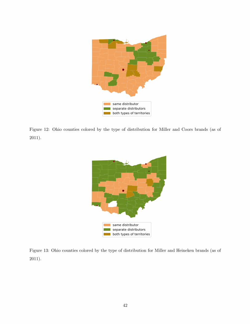
same distributorseparate distributorsboth types of territories
Figure 12: Ohio counties colored by the type of distribution for Miller and Coors brands (as of
2011).
same distributorseparate distributorsboth types of territories
Figure 13: Ohio counties colored by the type of distribution for Miller and Heineken brands (as of
2011).
42
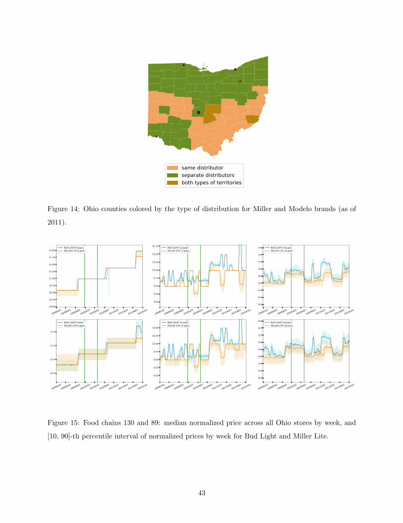
same distributorseparate distributorsboth types of territories
Figure 14: Ohio counties colored by the type of distribution for Miller and Modelo brands (as of
2011).
2009010120090501
2009090120100101
2010050120100901
2011010120110501
2011090120120101
10.00
10.25
10.50
10.75
11.00
11.25
11.50
11.75
12.00BUD LIGHT 6-packMILLER LITE 6-pack
2009010120090501
2009090120100101
2010050120100901
2011010120110501
2011090120120101
9.00
9.25
9.50
9.75
10.00
10.25
10.50
10.75 BUD LIGHT 12-packMILLER LITE 12-pack
2009010120090501
2009090120100101
2010050120100901
2011010120110501
2011090120120101
8.0
8.2
8.4
8.6
8.8
9.0
9.2
9.4
9.6 BUD LIGHT 24-packMILLER LITE 24-pack
2009010120090501
2009090120100101
2010050120100901
2011010120110501
2011090120120101
10.5
11.0
11.5
12.0
BUD LIGHT 6-packMILLER LITE 6-pack
2009010120090501
2009090120100101
2010050120100901
2011010120110501
2011090120120101
9.00
9.25
9.50
9.75
10.00
10.25
10.50
BUD LIGHT 12-packMILLER LITE 12-pack
2009010120090501
2009090120100101
2010050120100901
2011010120110501
2011090120120101
8.0
8.2
8.4
8.6
8.8
9.0
9.2
9.4
9.6 BUD LIGHT 24-packMILLER LITE 24-pack
Figure 15: Food chains 130 and 89: median normalized price across all Ohio stores by week, and
[10, 90]-th percentile interval of normalized prices by week for Bud Light and Miller Lite.
43

2009010120090501
2009090120100101
2010050120100901
2011010120110501
2011090120120101
10.25
10.50
10.75
11.00
11.25
11.50
11.75
12.00
12.25 BUD LIGHT 6-packMILLER LITE 6-pack
2009010120090501
2009090120100101
2010050120100901
2011010120110501
2011090120120101
9.00
9.25
9.50
9.75
10.00
10.25
10.50
10.75 BUD LIGHT 12-packMILLER LITE 12-pack
2009010120090501
2009090120100101
2010050120100901
2011010120110501
2011090120120101
7.8
8.0
8.2
8.4
8.6
8.8
9.0
9.2
9.4 BUD LIGHT 24-packMILLER LITE 24-pack
2009010120090501
2009090120100101
2010050120100901
2011010120110501
2011090120120101
11.0
11.5
12.0
12.5
13.0BUD LIGHT 6-packMILLER LITE 6-pack
2009010120090501
2009090120100101
2010050120100901
2011010120110501
2011090120120101
9.25
9.50
9.75
10.00
10.25
10.50
10.75
11.00BUD LIGHT 12-packMILLER LITE 12-pack
2009010120090501
2009090120100101
2010050120100901
2011010120110501
2011090120120101
8.0
8.2
8.4
8.6
8.8
9.0
9.2
9.4
9.6BUD LIGHT 24-packMILLER LITE 24-pack
Figure 16: Drug store chains 4901 and 4904: median normalized price across all Ohio stores by
week, and [10, 90]-th percentile interval of normalized prices by week for Bud Light and Miller Lite.
2009010120090501
2009090120100101
2010050120100901
2011010120110501
2011090120120101
10.5
11.0
11.5
12.0
BUD LIGHT 6-packMILLER LITE 6-pack
2009010120090501
2009090120100101
2010050120100901
2011010120110501
2011090120120101
9.00
9.25
9.50
9.75
10.00
10.25
10.50
10.75 BUD LIGHT 12-packMILLER LITE 12-pack
2009010120090501
2009090120100101
2010050120100901
2011010120110501
2011090120120101
8.0
8.2
8.4
8.6
8.8
9.0
9.2
9.4BUD LIGHT 24-packMILLER LITE 24-pack
2009010120090501
2009090120100101
2010050120100901
2011010120110501
2011090120120101
10.00
10.25
10.50
10.75
11.00
11.25
11.50
11.75
12.00 BUD LIGHT 6-packMILLER LITE 6-pack
2009010120090501
2009090120100101
2010050120100901
2011010120110501
2011090120120101
8.75
9.00
9.25
9.50
9.75
10.00
10.25
10.50BUD LIGHT 12-packMILLER LITE 12-pack
2009010120090501
2009090120100101
2010050120100901
2011010120110501
2011090120120101
7.8
8.0
8.2
8.4
8.6
8.8
9.0
9.2
9.4 BUD LIGHT 24-packMILLER LITE 24-pack
Figure 17: Mass merchandise chains 6901 and 6904: median normalized price across all Ohio stores
by week, and [10, 90]-th percentile interval of normalized prices by week for Bud Light and Miller
Lite.
44
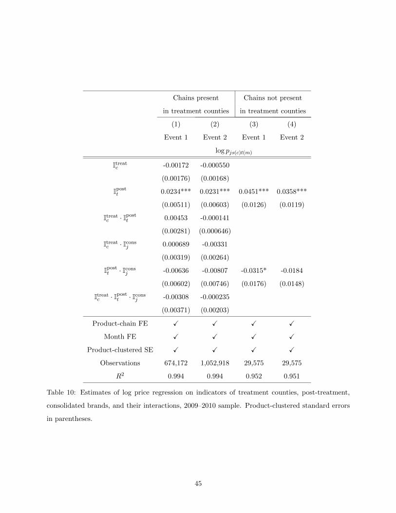
Chains present Chains not present
in treatment counties in treatment counties
(1) (2) (3) (4)
Event 1 Event 2 Event 1 Event 2
log pjs(c)t(m)
Itreatc -0.00172 -0.000550
(0.00176) (0.00168)
Ipostt 0.0234*** 0.0231*** 0.0451*** 0.0358***
(0.00511) (0.00603) (0.0126) (0.0119)
Itreatc · Ipost
t 0.00453 -0.000141
(0.00281) (0.000646)
Itreatc · Icons
j 0.000689 -0.00331
(0.00319) (0.00264)
Ipostt · Icons
j -0.00636 -0.00807 -0.0315* -0.0184
(0.00602) (0.00746) (0.0176) (0.0148)
Itreatc · Ipost
t · Iconsj -0.00308 -0.000235
(0.00371) (0.00203)
Product-chain FE X X X X
Month FE X X X X
Product-clustered SE X X X X
Observations 674,172 1,052,918 29,575 29,575
R2 0.994 0.994 0.952 0.951
Table 10: Estimates of log price regression on indicators of treatment counties, post-treatment,
consolidated brands, and their interactions, 2009–2010 sample. Product-clustered standard errors
in parentheses.
45
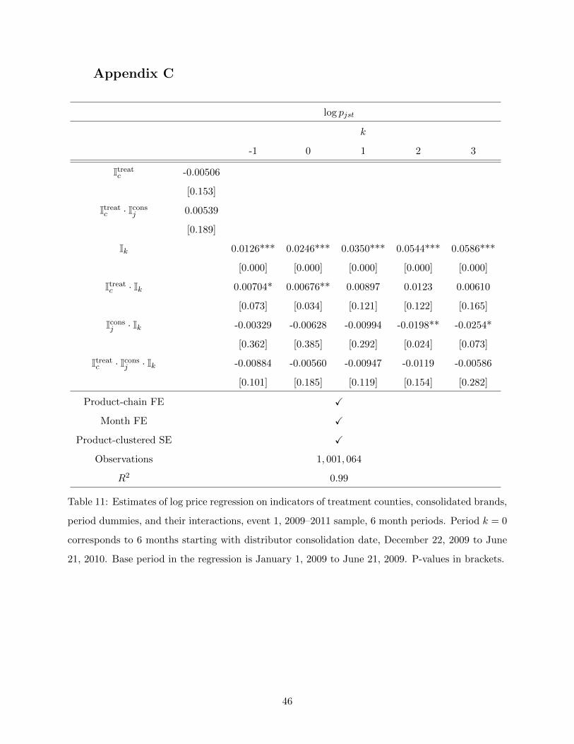
Appendix C
log pjst
k
-1 0 1 2 3
Itreatc -0.00506
[0.153]
Itreatc · Icons
j 0.00539
[0.189]
Ik 0.0126*** 0.0246*** 0.0350*** 0.0544*** 0.0586***
[0.000] [0.000] [0.000] [0.000] [0.000]
Itreatc · Ik 0.00704* 0.00676** 0.00897 0.0123 0.00610
[0.073] [0.034] [0.121] [0.122] [0.165]
Iconsj · Ik -0.00329 -0.00628 -0.00994 -0.0198** -0.0254*
[0.362] [0.385] [0.292] [0.024] [0.073]
Itreatc · Icons
j · Ik -0.00884 -0.00560 -0.00947 -0.0119 -0.00586
[0.101] [0.185] [0.119] [0.154] [0.282]
Product-chain FE X
Month FE X
Product-clustered SE X
Observations 1, 001, 064
R2 0.99
Table 11: Estimates of log price regression on indicators of treatment counties, consolidated brands,
period dummies, and their interactions, event 1, 2009–2011 sample, 6 month periods. Period k = 0
corresponds to 6 months starting with distributor consolidation date, December 22, 2009 to June
21, 2010. Base period in the regression is January 1, 2009 to June 21, 2009. P-values in brackets.
46
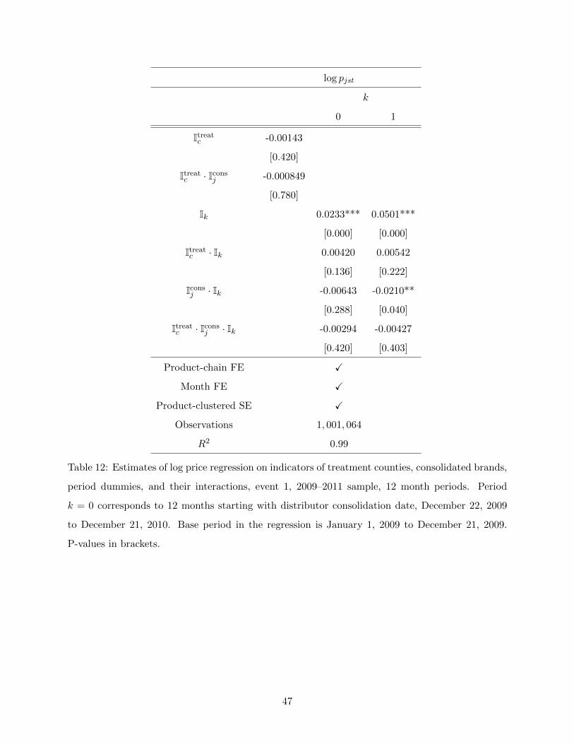
log pjst
k
0 1
Itreatc -0.00143
[0.420]
Itreatc · Icons
j -0.000849
[0.780]
Ik 0.0233*** 0.0501***
[0.000] [0.000]
Itreatc · Ik 0.00420 0.00542
[0.136] [0.222]
Iconsj · Ik -0.00643 -0.0210**
[0.288] [0.040]
Itreatc · Icons
j · Ik -0.00294 -0.00427
[0.420] [0.403]
Product-chain FE X
Month FE X
Product-clustered SE X
Observations 1, 001, 064
R2 0.99
Table 12: Estimates of log price regression on indicators of treatment counties, consolidated brands,
period dummies, and their interactions, event 1, 2009–2011 sample, 12 month periods. Period
k = 0 corresponds to 12 months starting with distributor consolidation date, December 22, 2009
to December 21, 2010. Base period in the regression is January 1, 2009 to December 21, 2009.
P-values in brackets.
47