Embed Size (px)
Citation preview
Distributed Multimedia
Synchronization Based on Fuzzy
Causal Relations
Por
Luis Alberto Morales Rosales
Tesis sometida como requisito parcial para obtener el grado de Doctor en Ciencias en la especialidad de Ciencias Computacionales en el Instituto Nacional de Astrofísica, Óptica y Electrónica.
Asesores:
Dr. Saúl Eduardo Pomares Hernández,
Dr. Gustavo Rodríguez Gómez,
Instituto Nacional de Astrofísica, óptica y Electrónica.
Sta. Ma. Tonantzintla, Puebla. 2009
INAOE 2009
Derechos Reservados El autor otorga al INAOE el permiso de reproducir y
distribuir copias de esta tesis en su totalidad o en partes

2
3
Summary
In this dissertation, the research is focused on the field of distributed multimedia systems
(DMS). One of the main problems in DMS is the data synchronization. Synchronization is
concerned with the preservation of temporal dependencies among the application data from
the time of generation to the time of presentation. The synchronization problem can be
characterized as an event ordering problem. Event ordering addresses the problem of
establishing a certain order among the events that occur in a distributed system (DS)
according to some particular criteria. The types of event orderings used in a DS are: no
order, FIFO, causal, ∆-causal, total, and causal-total. They mainly differ in the degree of
asynchronous execution allowed. One of the most important orderings is the causal order
(CO), which is based on Lamport’s happened-before relation. It establishes that the events
must be seen in the cause-effect order as they occur in the system. However, for certain
applications, for example multimedia synchronization, where some degradation of the
system is allowed, ensuring the CO based on Lamport’s relation is rigid and negatively
affects the performance of the system. In this dissertation a new ordering for DS is
introduced in order to achieve a more asynchronous execution than the CO. This new
ordering is called Fuzzy Causal Order (FCO). In addition, the Fuzzy Causal Relation (FCR)
and the Fuzzy Causal Consistency (FCC) are defined. The FCR establishes logical
dependencies based on the precedence of events and by considering some kind of
“distance” between their occurrences. With the notion of distance it was possible to
establish a cause-effect measure between two events a and b that indicates “how long ago”
an event a happened before an event b. Through the FCC, it was possible to determine
“how good” the performance of the system is at a given moment. The usefulness of the
FCO, FCR and FCC is shown by applying them to the concrete problem of intermedia
synchronization in DMS. In order to overcome the synchronization problem based on these
concepts, a distributed multimedia model and a synchronization algorithm were designed.
In addition, a fuzzy control system to adjust the delivery time of the messages and to
determine if a selective message discard must be carried out was designed.
4
Index
Index of Acronyms ................................................................................................................. 6
Chapter 1. Introduction ........................................................................................................... 7
1.1 Introduction .............................................................................................................. 7
1.2 Description of the problem .................................................................................... 10
1.3 Proposal of solution ............................................................................................... 12
1.4 Goals ...................................................................................................................... 13
1.5 Main contributions ................................................................................................. 14
1.6 Thesis organization ................................................................................................ 15
Chapter 2. State of the art ..................................................................................................... 17
2.1 Introduction ............................................................................................................ 17
2.2 Related work of multimedia synchronization ........................................................ 18
2.2.1 Synchronization on Demand .......................................................................... 18
2.2.2 Synchronization in real-time .......................................................................... 20
2.3 Synchronization Inter-streams ............................................................................... 21
2.3.1 Synchronous works ........................................................................................ 22
2.3.2 Asynchronous works ...................................................................................... 25
2.4 Fuzzy distributed multimedia synchronization ...................................................... 28
2.4.1 Fuzzy relation ................................................................................................. 28
2.4.2 Inter-stream synchronization using fuzzy logic concepts............................... 29
Chapter 3. Fuzzy Causal Ordering for Distributed Systems ................................................ 31
3.1 Introduction ............................................................................................................ 31
3.2 Preliminaries .......................................................................................................... 34
3.2.1 The System Model .......................................................................................... 34
3.2.2 Background and definitions ............................................................................ 35
3.3 Fuzzy causal relation and fuzzy causal consistency .............................................. 37
3.3.1 Fuzzy causal relation ...................................................................................... 37
3.3.2 Fuzzy causal consistency ................................................................................ 40
3.4 Fuzzy causal delivery for event ordering ............................................................... 41
3.5 Fuzzy causal order versus causal order .................................................................. 42
Chapter 4. Synchronization Model and Fuzzy Control for Multimedia Systems ................ 45
4.1 Introduction ............................................................................................................ 45
4.2 Multimedia synchronization model ....................................................................... 46
4.3 Component of input variables ................................................................................ 50
4.3.1 Causal distance ............................................................................................... 50
4.3.2 Temporal distance........................................................................................... 50
4.3.3 Duration of the synchronization period .......................................................... 51
4.3.4 Establishing the weighting grade (GP) ........................................................... 51
5
4.3.5 Determining the network conditions .............................................................. 53
4.4 Fuzzy causal component ........................................................................................ 55
4.4.1 The FCR applied to the intermedia synchronization ...................................... 55
4.4.2 The FCC applied to the intermedia synchronization ...................................... 58
4.5 Fuzzy control system ............................................................................................. 59
Chapter 5. Distributed Multimedia Synchronization Mechanism ........................................ 62
5.1 Introduction ............................................................................................................ 62
5.2 Distributed multimedia synchronization algorithm ............................................... 62
5.2.1 Algorithm codification ................................................................................... 63
5.3 General description of the algorithm ..................................................................... 68
5.4 Simulation .............................................................................................................. 69
5.4.1 Variables of the fuzzy control system ............................................................ 71
5.5 Results .................................................................................................................... 73
5.5.1 Soft case .......................................................................................................... 73
5.5.2 Medium case ................................................................................................... 76
5.5.3 Hard Case ....................................................................................................... 79
Chapter 6. Conclusions and Future Work ............................................................................ 82
6.1 Conclusions ............................................................................................................ 82
6.2 Future Work ........................................................................................................... 83
References ............................................................................................................................ 86
Appendixes ........................................................................................................................... 93
Appendix A. Happened-before relation for Intervals ........................................................... 93
Appendix B. Causal Distance Algorithm for Broadcast Case ............................................. 94
Appendix C. Maximum Error Tolerable for Multimedia Synchronization .......................... 97

6
Index of Acronyms Acronym or Symbol Definition
DS Distributed system DMS Distributed multimedia systems CO Causal order
FCR Fuzzy causal relation FCNR Fuzzy concurrent relation FCC Fuzzy causal consistency FCO Fuzzy causal order QoS Quality of service FR Frame rate GP Weighting grade NC Network conditions CS Current state of the system
RTT Round trip time of a message RS Spatial relation RT Temporal relation RL Logical relation DR Distance relation RN Membership function for the temporal distance RD Membership function for the causal distance → Causal relation || Concurrent relation
→λ
Fuzzy causal relation
λ
Fuzzy concurrent relation
EF Synchronization period
→I Happened before relation for intervals
||| Simultaneous interval relation
7
Chapter 1
“A problem is a chance for you to do your best.” Duke Ellington(1899-1974)
Introduction
1.1 Introduction
The advances of distributed systems over wide area networks has increased the research
interest of fields such as mobile system, ubiquitous computation and distributed multimedia
systems, among others.
In this dissertation the research is focused on the field of distributed multimedia systems
(DMS). The distributed multimedia systems have been defined as the exchange of big
volumes of multimedia data in a communication network among a group of participants
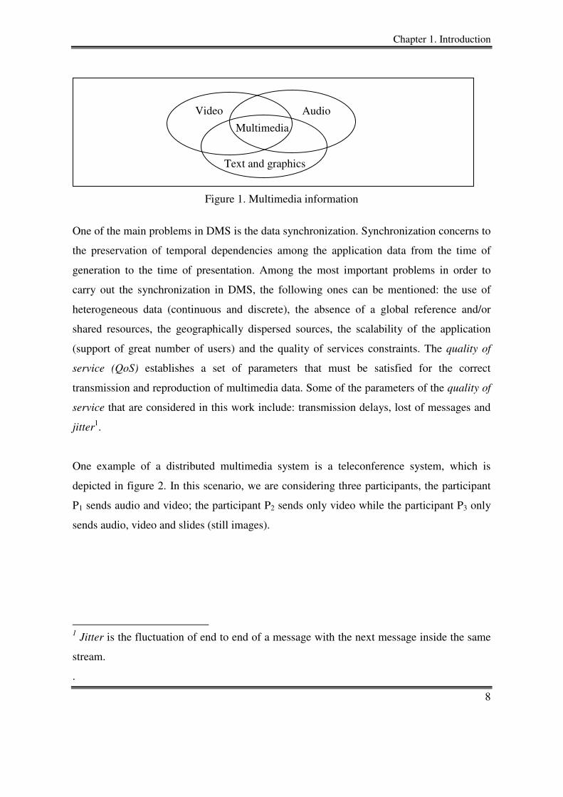
[20]. The term multimedia is defined as the integration and management of data represented
as continuous data (audio and video) and/or discrete data (text and graphics); see figure 1.
The management refers to the act of capturing, processing, communicating, storing and/or
presentation continuous and discrete data.
Chapter 1. Introduction
8
Figure 1. Multimedia information
One of the main problems in DMS is the data synchronization. Synchronization concerns to
the preservation of temporal dependencies among the application data from the time of
generation to the time of presentation. Among the most important problems in order to
carry out the synchronization in DMS, the following ones can be mentioned: the use of
heterogeneous data (continuous and discrete), the absence of a global reference and/or
shared resources, the geographically dispersed sources, the scalability of the application
(support of great number of users) and the quality of services constraints. The quality of
service (QoS) establishes a set of parameters that must be satisfied for the correct
transmission and reproduction of multimedia data. Some of the parameters of the quality of
service that are considered in this work include: transmission delays, lost of messages and
jitter1.
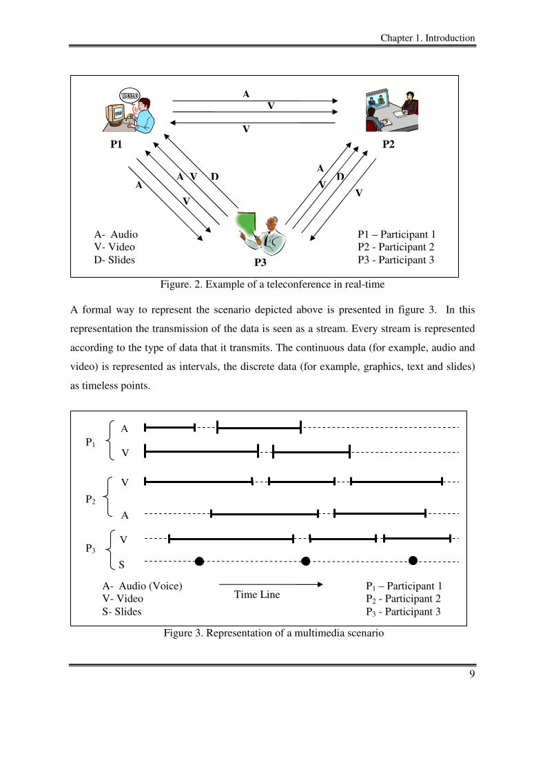
One example of a distributed multimedia system is a teleconference system, which is
depicted in figure 2. In this scenario, we are considering three participants, the participant
P1 sends audio and video; the participant P2 sends only video while the participant P3 only
sends audio, video and slides (still images).
1 Jitter is the fluctuation of end to end of a message with the next message inside the same
stream.
.
Audio Video
Text and graphics
Multimedia
Chapter 1. Introduction
9
Figure. 2. Example of a teleconference in real-time
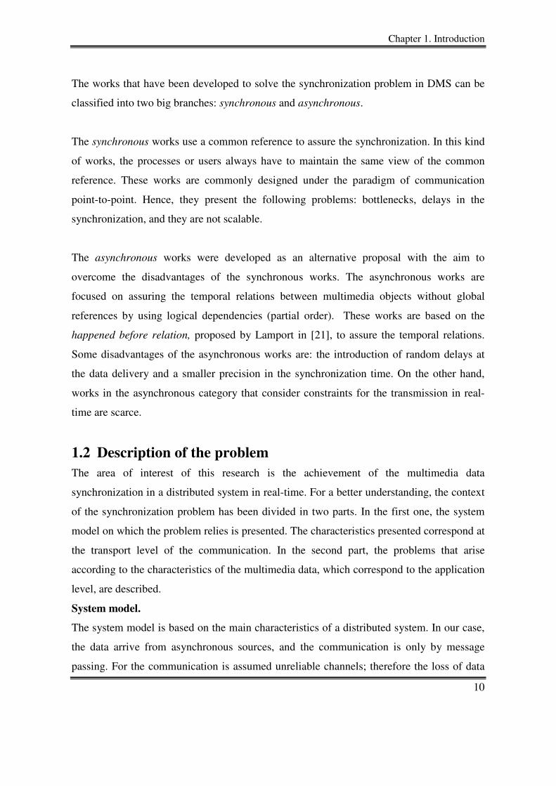
A formal way to represent the scenario depicted above is presented in figure 3. In this
representation the transmission of the data is seen as a stream. Every stream is represented
according to the type of data that it transmits. The continuous data (for example, audio and
video) is represented as intervals, the discrete data (for example, graphics, text and slides)
as timeless points.
Figure 3. Representation of a multimedia scenario
A
V
A
V
V
S
P1
P3
P2
A- Audio (Voice) V- Video S- Slides
P1 – Participant 1 P2 - Participant 2 P3 - Participant 3
Time Line
A
A
A
P1 P2
P3
V
V
A
V V
V V
D D
A- Audio V- Video D- Slides
P1 – Participant 1 P2 - Participant 2 P3 - Participant 3
Chapter 1. Introduction
10
The works that have been developed to solve the synchronization problem in DMS can be
classified into two big branches: synchronous and asynchronous.
The synchronous works use a common reference to assure the synchronization. In this kind
of works, the processes or users always have to maintain the same view of the common
reference. These works are commonly designed under the paradigm of communication
point-to-point. Hence, they present the following problems: bottlenecks, delays in the
synchronization, and they are not scalable.
The asynchronous works were developed as an alternative proposal with the aim to
overcome the disadvantages of the synchronous works. The asynchronous works are
focused on assuring the temporal relations between multimedia objects without global
references by using logical dependencies (partial order). These works are based on the
happened before relation, proposed by Lamport in [21], to assure the temporal relations.
Some disadvantages of the asynchronous works are: the introduction of random delays at
the data delivery and a smaller precision in the synchronization time. On the other hand,
works in the asynchronous category that consider constraints for the transmission in real-
time are scarce.
1.2 Description of the problem
The area of interest of this research is the achievement of the multimedia data
synchronization in a distributed system in real-time. For a better understanding, the context
of the synchronization problem has been divided in two parts. In the first one, the system
model on which the problem relies is presented. The characteristics presented correspond at
the transport level of the communication. In the second part, the problems that arise
according to the characteristics of the multimedia data, which correspond to the application
level, are described.
System model.
The system model is based on the main characteristics of a distributed system. In our case,
the data arrive from asynchronous sources, and the communication is only by message
passing. For the communication is assumed unreliable channels; therefore the loss of data
Chapter 1. Introduction
11
and random delays are considered in the network conditions. In the model a global clock is
not used nor are any other shared resources. Achieving the synchronization using the
system model described above, diverse questions arises. Two interesting question that can
be remarked are:
− How can one ensure the temporal dependencies among events arriving from
asynchronous sources in the presence of loss data and random delays?
− How can one ensure the temporal dependencies among events arriving from
asynchronous sources only by messages passing without having a common
reference like a physical global clock?
Multimedia data. The multimedia synchronization in distributed system is too correlated
with the data characteristics, which have been divided into two sections for their
explanation. In the first section some characteristics according how the data are generated
(in-line or off-line) are presented. In the second section the characteristics regarding to the
data heterogeneity (continuous and discrete) are explained.
• Data generation. Generally, the synchronization of multimedia data can be
classified in two categories according to the way the data are generated. The first
category refers to the synchronization on demand, where the data are previously
stored and labeled (off-line). The second category is known as synchronization in
real-time, where the data are generated in-line (they are neither stored nor pre-
labeled). The later is the focus of our study. An interesting challenge to carry out the
synchronization in real-time is:
− How it is possible to generate and label the data, without previous
knowledge of the system behavior, to assure the synchronization without
degrading the quality of the service?
• Heterogeneous data. The multimedia synchronization in distributed scenarios
handles heterogeneous data, which have been classified as discrete and continuous.
The characteristics of transmission of the continuous and discrete data are not
compatible. For example, the continuous data (audio and video) supports certain
losses but they are sensitive to delays; on the other hand the discrete data (graphics
and text) support certain delays but are sensitive to losses. Establishing a balance for
Chapter 1. Introduction
12
the delivery time among both types of data in a distributed scenario is not an easy
task, so the next question that arises is the following:
− How is a balance in the delivery time among heterogeneous data without
degrading the quality of service determined?
1.3 Proposal of solution
As hypothesis in this dissertation, it is claimed that for certain domains where some
degradation of the system is allowed, for example, as in the case of scheduling, and
intermedia synchronization, ensuring the causal order strictly based on Lamport’s relation
is still rigid, which can render negative affects to the performance of the system. In this
dissertation the research is focused on the domain of intermedia synchronization in
distributed multimedia systems. Specifically, in this domain the degradation can refer to the
synchronization error allowed among the multimedia data. The synchronization error
allowed is correlated with the type of media involved (continuous and/or discrete) and the
transmission mode (on-demand or real-time). In order to assure the synchronization and
allow an asynchronous execution of the system, some works have used the strict causal
order proposed by Lamport. Nevertheless, the use of this order can introduce the halt of the
system, discarded data and/or delivery delay of the data, which can result in a negative
system performance.
In order to demonstrate the hypothesis established above and carry out the intermedia
synchronization in DMS, a new event ordering for distributed systems is introduced, which
allows a more asynchronous execution than the causal order proposed by Lamport; this new
ordering is called Fuzzy Causal Order (FCO). The FCO is based on two new concepts, the
Fuzzy Causal Relation (FCR) and the Fuzzy Causal Consistency (FCC) for distributed
systems, which are defined in Chapter 3. The fuzzy causal relation establishes cause-effect
dependencies among events based not only on their precedence dependencies but also by
considering some kind of “distance” between the occurrences of the events. By using the
notion of “distance”, it aims to establish a cause-effect degree that indicates “how long

Chapter 1. Introduction
13
ago” an event a happened before an event b. Besides, the Fuzzy Causal Consistency is
based on the FCR. By considering some attributes of the addressed problem, it gives
information about “how good” the performance of the system is at a given moment. There
are two hypotheses behind this: first, according to the addressed problem, it is established
that “closer” events have a stronger cause-effect relation; and secondly, events with a
stronger cause-effect relation have a greater impact (negative or positive) on the
performance of the system. While the FCR is directly concerned with the first hypothesis,
the FCC deals with the second one.
As a direct result of the application of the FCO to the synchronization problem, a
synchronization mechanism for distributed multimedia systems in real-time is presented,
which is described in Chapter 4. In this research, a DMS is said to be in real-time if the data
processing time and its transmission are sufficiently small so that the data reception seems
instantaneous to a user; some examples of applications in real-time include: teleconference,
tele-inmersion and videoconference. The mechanism is classified in the asynchronous
category, and it is designed for group communication preserving the main characteristics of
a distributed system. The mechanism is based on a distributed synchronization model,
which is constructed using the fuzzy casual relation and the fuzzy causal consistency. In
order to adjust the delivery time of the data and to overcome the synchronization error, a
fuzzy control system is included as part of the mechanism.
1.4 Goals
The research presented in this dissertation had the following goals in order to provide a
direction to answer each question established at the description of the problem and to
demonstrate the hypothesis claimed.
General goal
To develop an intermedia synchronization mechanism for distributed multimedia systems
in real-time.
Chapter 1. Introduction
14
Specific goals
• To define the concepts of fuzzy causal relation, fuzzy causal consistency and fuzzy
causal ordering for distributed systems.
• To define a distributed synchronization model based on the concepts of fuzzy causal
relation and fuzzy causal consistency.
• To develop a synchronization mechanism based on the model previously defined,
considering the following:
o Transmission in real-time, considering arriving data from different sources,
heterogeneous data, and network conditions, such as loss of messages, jitter
and transmission random delays.
o Data transmission using the paradigm of group communication (two or more
participants) preserving the main characteristics of a distributed system.
1.5 Main contributions
The main contribution of this dissertation is the introduction of the following concepts:
fuzzy causal relation, fuzzy causal consistency and fuzzy causal ordering for distributed
systems. These concepts allow the establishment of a more asynchronous order than the
causal relation proposed by Lamport, as explained in Chapter 3.
As a result of the concepts proposed, a new synchronization model for distributed
multimedia systems was developed. This model showed the usefulness of the concepts in
order to solve problems where certain degradation of the system is allowed.
In addition, a new synchronization mechanism that carries out the synchronization model
was designed, which overcomes the main problems identified in the most of the works
designed for this end, including the halt of the system until the causal delivery is satisfied
(strict causal delivery), the discard of some messages that still can be useful for the
application (∆-causal delivery condition), and transmission random delays to deliver
messages. A fuzzy control system also was proposed to overcome the synchronization error
for distributed multimedia systems.
Chapter 1. Introduction
15
1.6 Thesis organization
Chapter 2 explains the state of the art, which is presented in two parts. The first part
includes the related work of multimedia synchronization; the works are classified according
to the way the data are generated, the type of synchronization, and the temporal and/or
logical dependencies used to carry out the synchronization. The second part presents how
fuzzy concepts have been used to solve the synchronization problem.
The main contribution of the research is presented in Chapter 3. This chapter contains the
definitions of Fuzzy Causal Relation (FCR) and Fuzzy Causal Consistency (FCC) for
distributed systems. Moreover, it introduces a new event ordering for distributed systems
based on the FCR and the FCC, which allows a more asynchronous execution than the
causal order proposed by Lamport; this new ordering has been called Fuzzy Causal Order
(FCO).
Chapter 4 presents the theoretical aspects of the distributed multimedia mechanism. The
mechanism is composed of four main components. First, the multimedia synchronization
model is presented, which establishes synchronization periods from the endpoints of the
intervals. Then, the component of the input variables used by the fuzzy causal consistency
and the fuzzy control system is described. After that, the fuzzy causal component shows the
application of the fuzzy causal relation and the fuzzy causal consistency to the intermedia
synchronization. The last component is the fuzzy control system, which adjusts the
messages delivery time and determines if a selective message discard must be carried out.
Chapter 5 describes the distributed multimedia mechanism. In addition, an algorithm that
carries out the model and the fuzzy control system is presented to show the usefulness of
the FCR and the FCC when applied to the intermedia synchronization problem. On the
other hand, some simulations and results of the behavior of the mechanism under several
conditions are presented.
Chapter 1. Introduction
16
Chapter 6 summarizes the main points of the dissertation and gives future directions of
research.
17
Chapter 2
“Study the past if you would define the future.” Confucius(551a.c.-479a.c.)
State of the art
2.1 Introduction
Recently, some internet applications (e.g. videoconferences and teleconference) involve
multimedia data and require enhancements in the performance of the data synchronization.
Several works have been developed to satisfy the data presentation in the same way that
they were sent from others participants (data synchronization). In this chapter, we give the
main differences of how the data synchronization is carried out according to the data
generation, on demand or in real-time. In addition, we describe how the temporal
dependencies, physical or logical, have been used to solve the synchronization problem.
The tendencies are focused on the use of logical dependencies. Hence, we describe the
main works based on logical dependencies, namely, causal and ∆-causal algorithms.
Finally, we explain the key works that have applied fuzzy concepts trying to solve the
multimedia synchronization problem.

Chapter 2. State of the art
18
2.2 Related work of multimedia synchronization
In this section, we describe the different approaches and mechanism that are used to solve
the synchronization. The synchronization works are divided based on how the data are
generated, on demand and real-time. In this research, we are mainly interested in the real-
time category. Inside this branch, there are two categories: the intra-stream, which is carried
out inside one stream, and the inter-stream, which is carried out among several streams in
order to maintain the coherence of the applications. Next, we are going to describe in detail
each one of the branches of the multimedia classification shown in figure 4.
Figure 4. Multimedia classification
2.2.1 Synchronization on Demand
The synchronization on demand is designed to satisfy temporal dependencies on
multimedia data that have been previously stored and labeled. With the synchronization on
demand, it is possible to previously establish the behavior of the continuous data (audio and
video) and/or discrete data (text, images) that will be presented, using information as the
duration and the data sequence. Examples of this type of synchronization can be found in
applications such as, on demand request of news or movies [7, 10, 17, 23]. The
synchronization on demand principally is realized by programming languages. The most
important of these will be described next.
Synchronization
On Demand Real-time
Intra-Stream Inter-Stream
Chapter 2. State of the art
19
Programming languages
One of the most common forms to carry out the synchronization on demand is by
programming languages. These languages are based on standards for multimedia
documents. The standards describe the form in which the data must to be synchronized. The
languages need to specify in advance the times of synchronization for all the cases that can
occur inside the system in order to obtain a good synchronization of the data. Among the
most outstanding languages are HyTime, MHEG, and SMIL. Next we will explain each one
of them.
The standard HyTime allows the structure description of multimedia documents. It is based
on SGML (Standard Generalized Markup Language [15]). HyTime contemplates a series of
primitives to connect multimedia objects without specifying its type of codification. The
primitive are declared in form of architectures (AF), and they are organized in modules.
The AFs are elements with predefined semantics and multimedia attributes. The modules
that define the basic concepts of HyTime are: Location-Address-Module, Finite-
Coordinate-Space-Module, Event-Projection-Module and Object-Modification-Module [15,
24].
MHEG is a standard oriented to multimedia documents. In MHEG a number of classes is
defined when the objects are created in order to design their presentation. There exist
several classes that are used to describe the form in which the video is opened, the audio
reproduction, the presentation and the grouping of the objects, the way of exchanging
information between machines, and the way the user can interact during the presentation.
The relations that are created between the instances of the classes determine the structure of
the presentation [41, 47].
SMIL (Synchronization Multimedia Language) is a standard to realize synchronization of
multimedia presentations in Internet. SMIL is defined by XML-DTD (Extensive Markup
Language Document Type Definitions [42]]). It defines the schedule of elements to describe
the temporal synchronization between multimedia elements. Likewise, it defines an element
Chapter 2. State of the art
20
of change to choose between the current alternative models and the quality of presentation
desired [30, 42].
2.2.2 Synchronization in real-time
The synchronization in real-time is characterized by the in-line data generation, which
implies that the data are neither previously stored nor pre-labeled. Among its main
characteristics, it can be mentioned that does not have a previously established time of
transmission and has not determined in advance the sequence of events that will be
presented along the transmission. In this category, we can find applications such as
videoconferences, distributed applications, cooperative work without tolerance delays, etc.
The synchronization in real-time can be divided into two categories, intra-stream and inter-
stream. The intra-stream synchronization refers principally to the preservation of physical
dependencies inside one stream. Some of the main works that have focused on solving the
synchronization intra-streams were proposed by Biersack et.al in [7], Haining et. al [10],
Hua et. al [13], and Tachikawa et. al [43].
In this dissertation the research is focused on the inter-stream synchronization. The next
sections present in detail which are their main characteristics as well as the way in which it
is carried out.
Inter-streams
The synchronization inter-streams, as opposed to the intra-streams synchronization, is
carried out to support logical and physical dependencies between different streams. This
type of synchronization becomes difficult to carry out when the streams come from
different sources. One of the open problems in this kind of synchronization relies on the
distributed environment, where there is neither shared resource nor a global clock. Some of
the mechanisms that have developed to solve the problems of the inter-stream
synchronization are based on temporal dependencies (physical time) and logical
dependencies (logical time). Sections 2.3 include detailed descriptions of some works that
have been developed using these kinds of dependencies. Due to the importance that this
category represents for the present dissertation, we dedicate the following section to present
its most important characteristics.

Chapter 2. State of the art
21
2.3 Synchronization Inter-streams
The inter-stream synchronization is concerned with maintaining the temporal and/or logical
dependencies among several streams in order to present the data in the same view as they
were generated. There are two main approaches that try to solve the inter-stream
synchronization; these are called synchronous and asynchronous. The difference among
these two approaches involves the asynchrony allowed for the system in order to maintain a
good performance of the system. We show in figure 5 the classification of the inter-stream
synchronization based on the temporal relations used and the grade of asynchrony of the
system.
Figure 5. Classification of the inter-stream synchronization
In order to explain the differences between the synchronous and asynchronous works, we
will first explain the temporal dependencies used by these works in order to solve the inter-
stream synchronization problem.
Temporal dependencies
The temporal dependencies are associated with physical time clocks to determine the event
ordering. The use of physical clocks facilitates the synchronization because the exact time
Inter-Stream
Synchronous Asynchronous
Logical Dependencies
Temporal Dependencies
Chapter 2. State of the art
22
in which the events happen is known. Nevertheless, synchronizing the clocks of the
involved sources is not an easy task, especially when this mechanism wants to be
established in a distributed system. There are two main ways to synchronize physical
clocks, either in a centralized or in a distributed way. In the centralized way the
synchronization task is delegated to a server; all the participants send their events to the
server and only the clocks between the server and each of the participants are synchronized
in order to establish the correct event delivery. We can find another example of this type of
synchronization when a multiplexor is used in the transmission of audio and video,
resulting in only one stream, labeling the resultant stream with a mark of a physical clock.
The centralized mechanism, although very simple, is not efficient since it introduces the
bottleneck effect and delays at the rebroadcasting of the events. On the other hand, in a
distributed environment it is difficult to support this type of clock synchronization because,
in this environment every clock is independent, and they do not work exactly at the same
speed. A way of carrying out the synchronization in distributed environments is using a
physical virtual time in order to allow all the participants to have the same time reference.
Logical dependencies
The temporal logical dependencies are associated with a logical time clock to label each
one of the events that occur in the system. In other words, they use a numerical labeling to
know the order in which the events occur in time. With the logical dependencies, the
bottleneck effect is avoided, but the random delays at the event delivery still remained. To
guarantee the delivery order of events, using logical dependencies, the mechanisms which
are the most used are the causal and the ∆-causal algorithms. These algorithms are used
when it is desirable to carry out the synchronization in a distributed environment.
Next, we will describe the synchronous and asynchronous works that use the temporal
dependencies presented above to solve the distributed multimedia synchronization.
2.3.1 Synchronous works
The synchronous works commonly use temporal physical dependencies and a common
reference to assure the synchronization. Some of the common references used for the data
Chapter 2. State of the art
23
labeling, resulting the correct order of delivery (process of synchronization), are the global
clocks (physical or virtual), shared memory, synchronization out of line, etc. [48, 51] In this
type of works, a view of the common reference is always maintained. These works are
commonly designed under the concept of communication point-to-point hence they have
the following problems: bottlenecks, delays in the synchronization and in addition they are
not scalable. The principal mechanisms developed under this characteristic are based on
centralized schemes, retransmission of information and pre-labeled data.
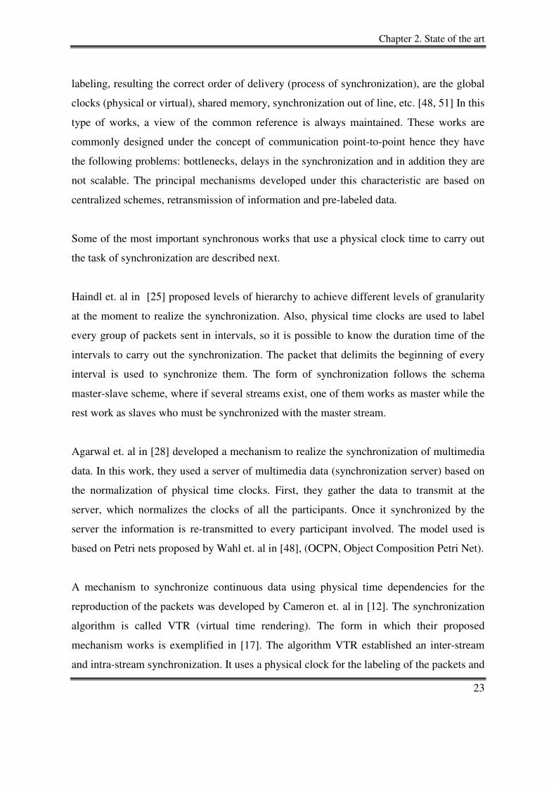
Some of the most important synchronous works that use a physical clock time to carry out
the task of synchronization are described next.
Haindl et. al in [25] proposed levels of hierarchy to achieve different levels of granularity
at the moment to realize the synchronization. Also, physical time clocks are used to label
every group of packets sent in intervals, so it is possible to know the duration time of the
intervals to carry out the synchronization. The packet that delimits the beginning of every
interval is used to synchronize them. The form of synchronization follows the schema
master-slave scheme, where if several streams exist, one of them works as master while the
rest work as slaves who must be synchronized with the master stream.
Agarwal et. al in [28] developed a mechanism to realize the synchronization of multimedia
data. In this work, they used a server of multimedia data (synchronization server) based on
the normalization of physical time clocks. First, they gather the data to transmit at the
server, which normalizes the clocks of all the participants. Once it synchronized by the
server the information is re-transmitted to every participant involved. The model used is
based on Petri nets proposed by Wahl et. al in [48], (OCPN, Object Composition Petri Net).
A mechanism to synchronize continuous data using physical time dependencies for the
reproduction of the packets was developed by Cameron et. al in [12]. The synchronization
algorithm is called VTR (virtual time rendering). The form in which their proposed
mechanism works is exemplified in [17]. The algorithm VTR established an inter-stream
and intra-stream synchronization. It uses a physical clock for the labeling of the packets and
Chapter 2. State of the art
24
calculates the time in which they must be reproduced based on the obtained information
from the sending time and the arrival time of the packets. This is done by using established
equations. The algorithm uses the concept master-slave, where a master stream is used to
synchronize the rest of the streams. An extension of these works was presented by Zhu et.
al in [13], where a ∆-causal is included control to determine the life time of the packets in
order to assure the packet delivery order. Nevertheless, they assumed that the clocks used
are globally synchronized.
A protocol to synchronize multimedia streams is presented Dommel et. al in [9]. This work
proposes a multipoint synchronization protocol (MSP). The mechanism is coordinated by
means of the physical time. Besides, it works for several groups and for several network
conditions by using multicast communication if it is available. MSP operates as a covering
service using a backbone to reference the nodes. The protocol is adaptable according to the
network conditions, and it uses the concept of virtual global clock.
Several standards have been proposed for the synchronization of multimedia data. Among
the most out-standing of these, we can mention the standard MPEG [50] and the standard
H.323 [29]. The main characteristic of both works is the use of a multiplexer to guarantee
the data synchronization. Therefore, both works present the disadvantage of introducing the
bottleneck effect and delays in the sending and reception time of the data.
Liu et. al in [10] developed a mechanism to carry out the data synchronization using a
virtual clock. They define equations that calculate the synchronization error in real-time
between the sender and receiver in order to indicate the adjustment of clocks to minimize
the error. Basically, the scheme of master- slave is used, where a master stream exists and
the rest of the streams are synchronized to the master.
Duda et. al in [4] presented a model that introduces the idea of a virtual observer
considering as hypothesis bounded delays in the network. The virtual observer defines the
temporal relations that must be preserved, whether these are inter-stream and intra-stream.
In this work the concept of multimedia presence is introduced to synchronize streams from
Chapter 2. State of the art
25
different sources. The multimedia presence refers to the set of streams produced or
controlled by a participant in a meeting. The algorithms proposed are adaptable and are
based upon the labeling of physical time to synchronize the streams. A global clock
synchronization of the participants is not assumed. Nevertheless, it is considered that all the
clocks advance at the same time. The model satisfies the intra-stream and inter-stream
synchronization for interactive applications in the Internet.
Another interesting protocol was proposed by Abouaissa et. al in [1]. In this work, a real-
time causal protocol that works in a distributed environment is presented. The ∆-causal
algorithm is used to realize the synchronization, which takes into account the lifetime of the
information. A characteristic of the protocol in order to assure the restrictions of real-time
is that it uses a main virtual physical time. At the beginning of the meeting all the clocks
are synchronized with the main clock; later the time of the main clock is sent periodically to
all the participants to continue with the synchrony of the clocks.
2.3.2 Asynchronous works
The asynchronous works arose as an alternative proposal that reduces the disadvantages of
the synchronous works. The asynchronous works are focused on assuring the temporal
relations between multimedia objects without global references by using logical
dependencies (partial order). Some disadvantages of the asynchronous works are: the
introduction of random delays at the data delivery and less precision in the synchronization
time. On the other hand, works in the asynchronous category that consider restrictions for
the transmission in real-time are scarce.
Next, we describe the main works based on logical dependencies (causal and ∆-causal
algorithms) to solve the synchronization problem.
A mechanism to identify causal relations between streams of information (audio, video, text
and images) was proposed by Courtiat in [16]. The mechanism is designed to assure the
causal relations expressed at a user level in order to guarantee which relations must be
preserved at the data delivery. The mechanism uses a global time and considers a master
Chapter 2. State of the art
26
stream, to which the other streams will have to be synchronized. The specification of the
mechanism is an extension of the formal description technique RT-LOTOS.
A causal algorithm for multimedia synchronization in real-time was presented by Baldoni
et. al in [34-37]. These works use a ∆-causal algorithm to satisfy time constraints. Among
the principal characteristics of these works is the use of a global clock to label the data in
order to determine the occurrence of the events. The ∆-causal algorithm, used to assure the
delivery order, labels the events with regard to a global time, which who know how the
events occurred in the system and who can determine a deadline for the delivery of the
events.
Tachikawa et. al defined a type of causality called ∆*-causality in [44]. This work is
focused on group communication for WAN environments. The ∆*-causality considers the
delay in the network, the data deadline and the order of occurrence of the events to
determine their precedence. In this work, every participant of the group needs to know the
delay and the loss rate of the events of all the participants; this is needed in order to
calculate the deadline of the data. Another characteristic is the retransmission of the data to
assure that they are received by all participants, which is possible to support the data loss.
A group communication protocol to synchronize continuous data in real-time was presented
by Tachikawa et. al in [45]. In this work, the protocol realizes a segment delivery based on
their causal dependencies determining a deadline for the delivery of the segments. In this
work a segment is composed of a sequence of packets. The synchronization is focus in
assuring the delivery according to the dependency between segments and not between
packets. A segment can be delivered at the application only until it has been completely
received. Nevertheless, they consider the loss of some packets of a segment. A
characteristic of the protocol is that all the participants have the same time in its physical
clock, which is viewed as a global clock to determine if a segment can be delivered
according to its deadline constraints.
Chapter 2. State of the art
27
Shimamura et. at in [38, 39] proposed some precedence relations called O- precedent,
which were designed on the object concept. In these works an object is composed by a
sequence of messages. They define six O-precedent relations: top - precede, tail - precede,
partially - precede, fully - precede, inclusive, precede and exclusively precede. These
relations contemplate the send and receive events of the objects as well as their beginning
and end to determine each one of the relations. They proposed a protocol to synchronize
multimedia objects among a group of participants, called COM (causally ordered
multimedia). The protocol is based on the O-precedent relations. In the protocol, the objects
are delivered to the application until they have received all the messages that compose them
and their delivery order established. The order of delivery is established by the relations O-
precedent. The extension to these works was developed by Enokido in [49]. In this case, the
extension includes relations for the cases: multicast (a message is sent to multiple sources),
parallel-cast (different messages are sent at the same time to different sources),
conjunctive-receipt (the destination will be blocked until all the messages are received from
all the sources) and disjunctive-receipt (the destination will be blocked until a message is
received from at least a source of objects). Another extension to the work of Shimamura
was proposed by Timura in [52]. The extension introduces a synchronization message to
segment an object. This message can be sent periodically or in any moment to realize the
segmentation. With the synchronization message, the object segmented is delivered to the
application without the need to wait until the object is completely received.
Morales et. al in [26, 27] proposed an algorithm to synchronize continuous data in real
time. The algorithm was designed using a synchronization model, which is based on an
extension to Lamport’s happened-before relation applied on interval level. The
synchronization is achieved with base on their logical dependencies among intervals. In
order to reach the continuous media synchronization, they work at two levels. At a higher
level, a stream is represented as an interval. At a lower level, an interval is defined as a
finite set of sequential discrete events. The work is focused on the lower level, where it was
shown that it is sufficient to ensure a partial order between some single events (endpoints
intervals) to ensure the causal order on interval level. In order to minimize the control
overhead, they proposed an extension of the Immediate Dependency Relation applied on
Chapter 2. State of the art
28
interval level. Some of the characteristics of the algorithm include the absence of a global
clock and assumption of reliable communication channels. Nevertheless, they consider
random delays at the data transmission.
2.4 Fuzzy distributed multimedia synchronization
This section is presented in two parts. In the first one, the main works that include the
concept of fuzzy relation are explained. The second one includes the works that have used
some concepts of fuzzy logic in order to solve the problem of inter-stream synchronization.
2.4.1 Fuzzy relation
The fuzzy relation is widely used in the fuzzy logic area. This relation indicates in a broad
sense the degree of compatibility among two concepts. The first work to introduce the
concept of fuzzy causal relation deals with the Fuzzy Cognitive Maps to establish a fuzzy
causal relation, and a degree of affectation among events or concepts of the system. Fuzzy
cognitive maps (FCM) are fuzzy weighted directed graphs with feedback that create models
that emulate the behavior of complex process using fuzzy causal relations, see Aguilar, [2].
However, the concept of fuzzy causal relation used for the FCM cannot apply for the event
ordering in distributed systems because to construct the fuzzy weighted directed graph for a
system, the degree of affectation of all events in the system must be known. It should be
observed that the FCMs are constructed off-line.
Badaloni and Giacomin in [40] integrate ideas of flexibility and uncertainty into Allen’s
interval-based temporal logic and define an interval fuzzy algebra IAfuzz. This work deals
with the qualitative aspect of temporal knowledge for the solution of planning problems
and prioritized constraints to express the degree of satisfaction needed. They just label the
different relations among intervals with a degree of satisfaction that the search of the
solution must satisfy. In addition, they must also know in advance the behavior and the
relations of the system, so the interval fuzzy algebra cannot apply for the event ordering in
distributed systems.
Chapter 2. State of the art
29
2.4.2 Inter-stream synchronization using fuzzy logic concepts
Some of the main works that have included concepts of fuzzy logic in distributed systems
are focused on trying to solve the multimedia synchronization problem on demand, which
consists in assuring the temporal appearance order of the data at the reception of every
participant as they were sent. This problem is in essence an event ordering problem. It is
important to remark that none of these works have developed the concepts of fuzzy causal
relation neither the fuzzy causal consistency for distributed systems, nor a solution that can
be applied for the synchronization in real time using fuzzy concepts in a DMS as it is
presented in this work.
Zhou and Murata in [54] presented a temporal petri-net model called Extended Fuzzy
Timing Net for distributed multimedia synchronization. Among their main characteristics,
they contemplate temporal uncertain requirements, making a measurement of the quality of
services parameters required by the application in order to check if they are satisfied. They
use a trapezoidal membership function to calculate and to know if the data are synchronized
(e.g. audio and video). The model is based on the concept of master-slave to carry out the
synchronization. Extended Fuzzy Timing Net model needs a set of forward relations
between multimedia objects, which are specified by the designer of the application.
Janakiraman et al. in [32, 33] give algorithms for the broadcasting of video on demand. In
this work, the fuzzycast concept is introduced and consists in determining the delivery order
of data based on the technique of the nearest neighbor taking account the generation time of
data. They use parameters such as available bandwidth, transmission delay, buffer space
and a server for the data transmission to all the participants of the group.
Coelho et. al in [3] presented a methodology for the high level specification and
decentralized coordination of temporal interdependences among objects of multimedia
documents. In this work, they introduced the use of the causality to establish fuzzy rules to
realize the multimedia synchronization. Nevertheless, they did not propose a fuzzy causal
relation for event ordering events in distributed systems; they used the causal relation
proposed by Lamport. The main characteristics of their work are: the specification is
Chapter 2. State of the art
30
realized by the user using fuzzy scripts, indicating how the events will have to be
synchronized. In addition, they classify the entities that compose the scenes to verify the
consistency of their temporal relations and have to indicate explicitly the synchronization
mechanism that will be associated with every multimedia entity. The fuzzy parameters for
the synchronization are also explicitly defined by the designer of the application. They use
a global reference to determine the synchronization time, as well as a producer-consumer
scheme to establish synchronization points. The specification is made offline, so the
desirable behavior of the objects reproduction has to be defined in advance.
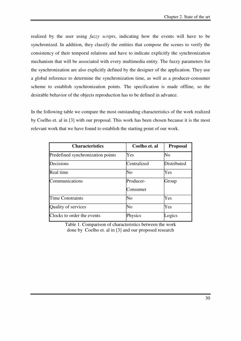
In the following table we compare the most outstanding characteristics of the work realized
by Coelho et. al in [3] with our proposal. This work has been chosen because it is the most
relevant work that we have found to establish the starting point of our work.
Characteristics Coelho et. al Proposal
Predefined synchronization points Yes No
Decisions Centralized Distributed
Real time No Yes
Communications Producer-
Consumer
Group
Time Constraints No Yes
Quality of services No Yes
Clocks to order the events Physics Logics
Table 1. Comparison of characteristics between the work done by Coelho et. al in [3] and our proposed research
31
Chapter 3
“The significant problems we have cannot be solved at the same level of thinking with which we created them.”
Albert Einstein(1879-1995)
Fuzzy Causal Ordering for
Distributed Systems
3.1 Introduction In a distributed system (DS), it is not always feasible in practice to synchronize physical
time across different processes within the system in order to realize the event ordering.
Hence, the processes can use the concept of a logical clock based on the events through
which they communicate to establish the events ordering. A logical clock is a mechanism
for capturing chronological and causal relationships between events in a distributed system.
In DS there are three kinds of events: internal, send and receive events. The internal events
occur inside a process, and they are never known by the rest of the processes. On the other
hand, the send and receive events are those through which the processes communicate and
Chapter 3. Fuzzy Causal Ordering for Distributed Systems
32
cooperate. In this dissertation, only the send and receive events are considered since they
modify the global state of a system.
The event ordering in a DS consists in establishing a certain order among the events that
occur according to some particular criteria. According to the chosen criteria, the resulting
event ordering allows a greater or smaller degree of asynchronous execution. There are two
broad categories for event ordering used in distributed systems: total ordering and partial
ordering.
For total ordering, there are two variants: total-causal order and total order. The total-
causal order is the strictest ordering in a distributed system; it establishes only one
linearization, consistent with the causal ordering, among all the events that occur in the
system, even those that occur concurrently. For that reason, the execution of the system is
considered as synchronous. On the other hand, the total order establishes a sequential order
for all the events that occur in the system without ensuring the causal order.
The partial ordering presents two variants: the causal order proposed by Birman [5] and the
∆-causal order proposed by Baldoni [34-37]. Both of them are exclusively based on the
happened-before relation defined by Lamport [21]; the main difference is that the ∆-causal
considers that the events have an associated lifetime. The causal order establishes that for
each participant in the system the events must be seen in the cause-effect order as they have
occurred, whereas the ∆-causal order establishes that the events must be seen in the cause-
effect order only if the cause has been seen before its lifetime expires. Otherwise, the
cause-effect is considered to be broken, and therefore inexistent.
Partial ordering is important since it allows that the ordering view concerning the set of
events E of a system to differ among the participants; however, it does ensure that for a
subset of events E’∈ E, all participants will have the same consistent view according to the
chosen criteria. The smaller is E’, and the fewer ordering constraints are required, the more
asynchronous is the system since there are less events to order and less constraints between
the events to accomplish. It is important to note that no type of event ordering is better than
Chapter 3. Fuzzy Causal Ordering for Distributed Systems
33
another. Each event ordering is meant to be used in a particular type of problem, where it
ensures the necessary ordering so as to satisfy its consistency constraints.
In this dissertation, it is claimed as hypothesis that for certain domains, such as scheduling,
planning, and intermedia synchronization, where some degradation of the system is
allowed, ensuring the causal order strictly based on Lamport’s relation is still rigid, which
can render negative affects to the performance of the system (e.g. the halt of the system,
discarded data and delivery delay of the event). The allowed degradation differs in each
domain according to the problem to solve. For example, in the scheduling domain for
complex problems, optimal schedulers are computationally heavy, and in some cases it is
practically impossible to construct them. In these cases, it is preferable to use a near-
optimal scheduling, which ensures a minimum of application requirements, such as
bandwidth, access time, and lost rate. In the planning domain, sometimes it is not possible
to carry out the entire set of tasks since they have some conflict among them. Therefore a
planner can identify what tasks must be executed in order to satisfy the maximum number
of constraints, and therefore, maximize the performance of the system. In the domain of
intermedia synchronization, the degradation can refer to the synchronization error allowed
among the multimedia data. For example, the synchronization error for a dialogue among
participants (audio-audio streams in real time) is acceptable if it is within ±120ms.
In this chapter, it is introduced a new event ordering for distributed systems that allows a
more asynchronous execution than the causal order proposed by Lamport; this new
ordering is called Fuzzy Causal Order (FCO). The FCO is based on the fuzzy causal
relation (FCR) and the fuzzy causal consistency (FCC) that will be defined in the following
sections. The fuzzy causal relation establishes cause-effect dependencies among events
based not only on their precedence dependencies but also by considering some kind of
“distance” between the occurrences of the events. By using the notion of “distance”, it aims
to establish a cause-effect degree that indicates “how long ago” an event a happened before
an event b. Besides, the fuzzy causal consistency is based on the FCR, by considering some
attributes of the addressed problem, it gives information about “how good” the performance
of the system is at a given moment. There are two hypotheses behind this: first, according

Chapter 3. Fuzzy Causal Ordering for Distributed Systems
34
to the addressed problem, it is established that “closer” events have a stronger cause-effect
relation; and secondly, events with a stronger cause-effect relation have a greater impact
(negative or positive) on the performance of the system. While the FCR is directly
concerned with the first hypothesis, the FCC deals with the second one.
The usefulness of the fuzzy causal order is showed in chapter 4 by applying it to the
concrete problem of intermedia synchronization in a distributed multimedia system (DMS),
where a certain synchronization error in the system is allowed according to the type of
media involved whether it is continuous and/or discrete, as well as the transmission mode
(on-demand, or real-time).
3.2 Preliminaries
Some basic definitions are described in this section in order to understand the fuzzy causal
relation. In addition, these definitions are used to clarify the main differences between the
strict causal relation, the ∆-causal relation and the fuzzy causal relation.
3.2.1 The System Model
Processes. The application under consideration is composed of a set of processes P={i,
j…} organized into a group that communicate by broadcast asynchronous messages
passing. In this case, the members of the group g are defined as Memb(g)=P.
Messages. The system considers a finite set of messages M, where each message m∈M is
identified by a 2-tuple (participant, integer), m=(p,x) where p∈P is the sender of m,
denoted by Src(m), x is the local logical clock for messages of p, when m is broadcasted.
The set of destinations Dest(m) of message m is composed of the participants connected to
the Group(Dest(m)=Memb(g)). The messages sent by the process p are denoted by Mp ={
m∈M : Src(m) = p }.
Events. Let m be a message, it is denoted by send(m) the emission event of m by Src(m),
and by delivery(p,m) the delivery event of m to participant p connected to Group(m). The
set of events associated to M is then the set E = {send(m) : m∈M} ∪ {delivery(p,m) : m ∈
Chapter 3. Fuzzy Causal Ordering for Distributed Systems
35
M ∧ p ∈Dest(m)}. An emission event send(m) where m=(p,x) may also be denoted by
send(p,m) or send(m) without ambiguity. The subset Ep⊆E of events involving p is Ep=
{send(m) : k=Src(m)} {delivery(p,m) : p∈Dest(m)}.
Intervals. Let I be a finite set of intervals, where each interval A∈I is a set of messages
A⊆M sent by a participant p=Part(A) defined by the mapping Part:I→P. Formally, m∈A
⇒Src(m)=Part(A). Owing to the sequential order of Part(A for all m, m’ ∈ A , m → m’ or
m’ → m. Let a- and a+ be the endpoint messages of A, such that for all m ∈ A : a-≠m and
a+≠m implies that a-→m→ a+.
3.2.2 Background and definitions
Happened-before relation proposed by Lamport
Lamport in [21] proposed the happened-before relation for events ordering in DS. With the
introduction of the happened-before relation was possible to maintain the synchronization,
coordination and/or consistency between events in a fully distributed manner. Some of the
important hypotheses of Lamport’s work are: the delivery time of the events is considered
finite but unbounded and there is not message loss. The happened-before relation also
known as causal relation was defined as follows:
Definition 1. The causal relation “→” is the least partial order relation on the set E that
satisfies the three following conditions:
• If a and b are events belonging to the same process and a was originated before b then
a→b.
• If a is the send message of a process and b is the reception of the same message in another
process, then a→b.
• If a→b and b→c then a→c.
By using “→”, Lamport defines that two events are concurrent as follows:
a || b if ¬ (a→b ∨ b→a)
Chapter 3. Fuzzy Causal Ordering for Distributed Systems
36
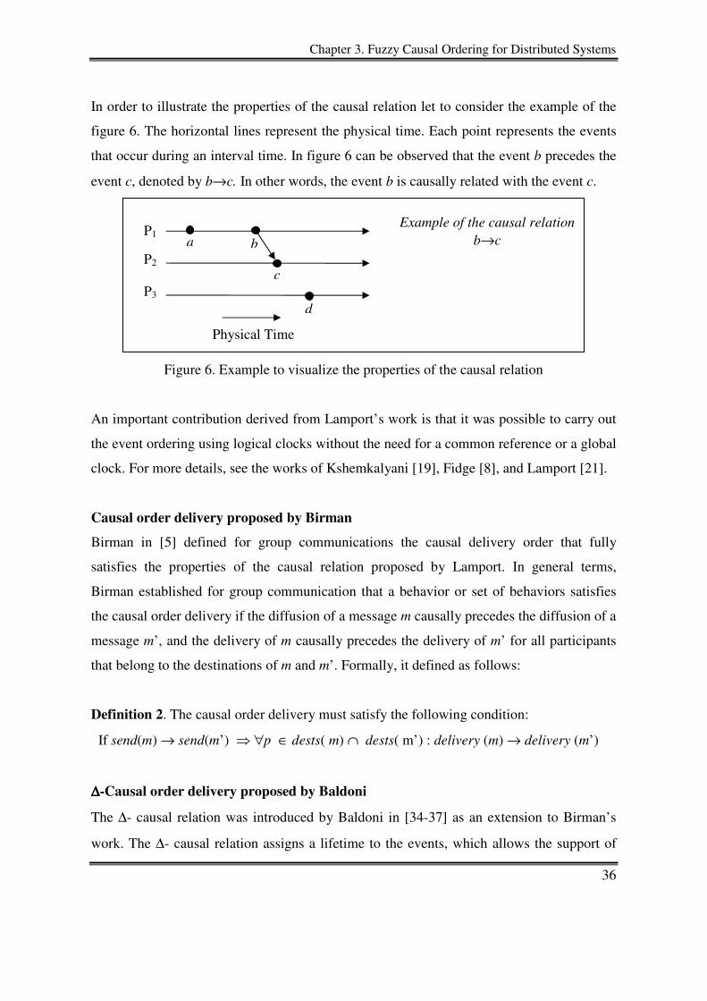
In order to illustrate the properties of the causal relation let to consider the example of the
figure 6. The horizontal lines represent the physical time. Each point represents the events
that occur during an interval time. In figure 6 can be observed that the event b precedes the
event c, denoted by b→c. In other words, the event b is causally related with the event c.
Figure 6. Example to visualize the properties of the causal relation
An important contribution derived from Lamport’s work is that it was possible to carry out
the event ordering using logical clocks without the need for a common reference or a global
clock. For more details, see the works of Kshemkalyani [19], Fidge [8], and Lamport [21].
Causal order delivery proposed by Birman
Birman in [5] defined for group communications the causal delivery order that fully
satisfies the properties of the causal relation proposed by Lamport. In general terms,
Birman established for group communication that a behavior or set of behaviors satisfies
the causal order delivery if the diffusion of a message m causally precedes the diffusion of a
message m’, and the delivery of m causally precedes the delivery of m’ for all participants
that belong to the destinations of m and m’. Formally, it defined as follows:
Definition 2. The causal order delivery must satisfy the following condition:
If send(m) → send(m’) ⇒ ∀p ∈ dests( m) ∩ dests( m’) : delivery (m) → delivery (m’)
∆∆∆∆-Causal order delivery proposed by Baldoni
The ∆- causal relation was introduced by Baldoni in [34-37] as an extension to Birman’s
work. The ∆- causal relation assigns a lifetime to the events, which allows the support of
P1 a b
c
d
Example of the causal relation b→c
P2
P3
Physical Time
Chapter 3. Fuzzy Causal Ordering for Distributed Systems
37
loss of messages, by preserving the order of precedence established by Lamport. The ∆-
causal delivery is formally defined as:
Definition 3. A distributed computation Ê respects a ∆-causal order if:
• All the messages M(Ê) that arrive in ∆ are delivered in ∆, all others are never delivered
(they are considered to be lost or discarded);
• All the events of delivery respect a causal order.
Where Ê=(E,→) is a set of events partially ordered (send and delivery) and M(Ê) is the set
of all the messages exchanged in Ê.
3.3 Fuzzy causal relation and fuzzy causal consistency
In this section, are introduced the fuzzy causal relation (FCR) and the fuzzy causal
consistency (FCC) for distributed systems. These can allow a more asynchronous execution
than the causal order proposed by Lamport; this new ordering is called Fuzzy Causal
Ordering and will be defined in the following section.
3.3.1 Fuzzy causal relation
The fuzzy causal relation (FCR) is denoted by “a →λ b”. The FCR is based on a notion
of “distance” among the events. The distance, according to the addressed problem, can be
established considering three main domains: spatial, temporal and/or logical. The reference
for the logical domain is the event ordering based on Lamport’s relation. Using the notion
of distance, the FCR establishes a cause-effect degree that indicates “how long ago” an
event a happened before an event b.
The distance between events is determined by the fuzzy relation DR: E × E → [0, 1], which
is established from the union of sets of membership functions, RS (spatial), RT (temporal),
and RL (logical), one set for each domain. It is formally defined as follows:
DR(a,b) = RS(R1 ∪ R2∪... Ro) ∪ RT(R1 ∪ R2∪... Rr)∪ RL(R1 ∪ R2∪... Rs)
Chapter 3. Fuzzy Causal Ordering for Distributed Systems
38
The number of membership functions, R, by each domain is determined according to the
problem to resolve. The fuzzy union operator chosen for intra and inter domains is the max
operator max(R1,..., Rk).
In this dissertation, one hypothesis considered for the FCR is that “closer” events have a
stronger cause-effect relation, according to the addressed problem. For this reason, it is
established that the DR grows monotonically and it is directly proportional to the spatial,
temporal and/or logical distances between a pair of events. This means, for example, that a
DR(a,b) with a value tending to zero indicates that the events a and b are “closer”.
It is important to remark that the DR cannot determine precedence dependencies among
events, it only indicates certain distance among them. For example, the value of the
distance between the events a and b gives an equal value for DR(a,b) or DR(b,a) because
the distance relation is not considering the precedence among them. Hence, in order to
establish a cause-effect degree (fuzzy precedence) among events, the Fuzzy Causal Relation
is formally defined by using the values of the DR as follows:
Definition 4. The fuzzy causal relation “ →λ ” on a set of events E satisfies the two
following conditions:
a →λ b If a→b ∧ 0 ≤ DR(a,b) < 1
a →λ c If ∃b a→b→c ∧ DR(a,b) ≤ DR(a,c) : DR(a,b), DR(a,c) < 1
The first condition establishes that two events (a, b) are fuzzy causal related if a happened
before b and the value of the DR(a,b) is smaller than one. The second condition is the
transitive property. This condition establishes that two events (a, c) are fuzzy causal related
if there exists an event b such that a happened before b, and b happened before c.
Moreover, the values for DR(a,b), DR(a, c) monotonically grow and they are smaller than
one. If any of these conditions are satisfied, the value of the DR(a,b) determines the cause-
effect degree between the present pair, and it is represented by FCR(a,b). In any case when
Chapter 3. Fuzzy Causal Ordering for Distributed Systems
39
the value of the DR(a, b) is equal one, this means that the events do not have a cause-effect
relation.
By using Lamport’s relation, a pair of events are concurrent if ¬ (a→b ∨ b→a), expressed
as “a || b”. In this work, based on the value of the DR, the concept of Fuzzy Concurrent
Relation (FCNR) is formally defined as:
Definition 5. Two events are fuzzy concurrent “ a λ b ”, if the following condition is
satisfied:
a λ b If ¬ (a→b ∨ b→a) ∧ ( (DR(a, b)= DR(b, a) ) < 1)
A fuzzy concurrent relation among two events exists if the events are concurrent and the
values of their DR are equal and less than the unit, which is represented as FCNR(a, b).
This means, that it can establish spatial and/or temporal relation(s) among the events even
when a logical precedence relation cannot be determined. It is observed that when the DR
for a pair of concurrent events (a, b) is equal and less than one, this means that the event a
has some effect on the event b and viceversa. Hence, for fuzzy concurrent events, a and b,
the order (a, b) or (b, a) is indistinct for the system.
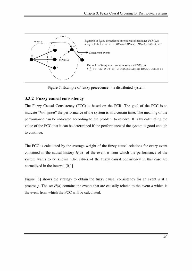
To illustrate the use of the FCR and the FCNR, consider the example given in Figure 7,
which shows a scenario to determine the fuzzy precedence and the fuzzy concurrency
between events. For example, for the case of the relation among the events a and e, the
FCR(a, e) determine if a cause-effect relation exist that must be taken into account for the
event ordering . For the fuzzy concurrent events e and b, the FCNR(c, e) identifies that
there is certain spatial and/or temporal relation between them.
Chapter 3. Fuzzy Causal Ordering for Distributed Systems
40
Figure 7. Example of fuzzy precedence in a distributed system
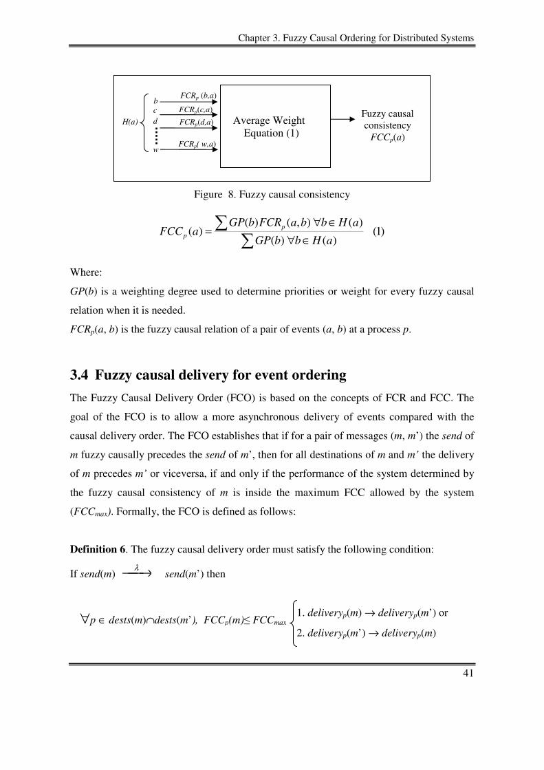
3.3.2 Fuzzy causal consistency
The Fuzzy Causal Consistency (FCC) is based on the FCR. The goal of the FCC is to
indicate “how good” the performance of the system is in a certain time. The meaning of the
performance can be indicated according to the problem to resolve. It is by calculating the
value of the FCC that it can be determined if the performance of the system is good enough
to continue.
The FCC is calculated by the average weight of the fuzzy causal relations for every event
contained in the causal history H(a) of the event a from which the performance of the
system wants to be known. The values of the fuzzy causal consistency in this case are
normalized in the interval [0,1].
Figure [8] shows the strategy to obtain the fuzzy causal consistency for an event a at a
process p. The set H(a) contains the events that are causally related to the event a which is
the event from which the FCC will be calculated.
Example of fuzzy precedence among causal messages FCR(a,e) a e If ∃b a→b→e ∧ DR(a,b) ≤ DR(a,e) : DR(a,b), DR(a,e) ) < 1
λ →
Example of fuzzy concurrent messages FCNR(c,e) b c If ¬ (a→b ∨ b→a) ∧ DR(b,c) = DR(c,b) : DR(b,c), DR(c,b) < 1
FCR(a,e)
a
b
c
d
e
f
FCNR(c,e)
Concurrent events
= λ
Chapter 3. Fuzzy Causal Ordering for Distributed Systems
41
Figure 8. Fuzzy causal consistency
)1()()(
)(),()()(
aHbbGP
aHbbaFCRbGPaFCC p
p ∈∀∈∀
=∑
∑
Where:
GP(b) is a weighting degree used to determine priorities or weight for every fuzzy causal
relation when it is needed.
FCRp(a, b) is the fuzzy causal relation of a pair of events (a, b) at a process p.
3.4 Fuzzy causal delivery for event ordering
The Fuzzy Causal Delivery Order (FCO) is based on the concepts of FCR and FCC. The
goal of the FCO is to allow a more asynchronous delivery of events compared with the
causal delivery order. The FCO establishes that if for a pair of messages (m, m’) the send of
m fuzzy causally precedes the send of m’, then for all destinations of m and m’ the delivery
of m precedes m’ or viceversa, if and only if the performance of the system determined by
the fuzzy causal consistency of m is inside the maximum FCC allowed by the system
(FCCmax). Formally, the FCO is defined as follows:
Definition 6. The fuzzy causal delivery order must satisfy the following condition:
If send(m) →λ send(m’) then
1. deliveryp(m) → deliveryp(m’) or
2. deliveryp(m’) → deliveryp(m)
Average Weight Equation (1)
c
d
w
FCRp (b,a) b
H(a) Fuzzy causal consistency
FCCp(a)
FCRp(c,a)
FCRp(d,a)
FCRp( w,a)
∀p ∈ dests(m)∩dests(m’), FCCp(m)≤ FCCmax
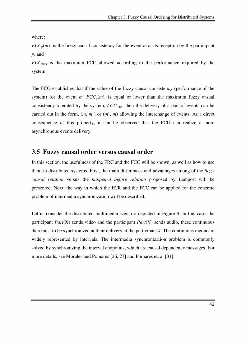
Chapter 3. Fuzzy Causal Ordering for Distributed Systems
42
where:
FCCp(m) is the fuzzy causal consistency for the event m at its reception by the participant
p, and
FCCmax is the maximum FCC allowed according to the performance required by the
system.
The FCO establishes that if the value of the fuzzy causal consistency (performance of the
system) for the event m, FCCp(m), is equal or lower than the maximum fuzzy casual
consistency tolerated by the system, FCCmax, then the delivery of a pair of events can be
carried out in the form, (m, m’) or (m’, m) allowing the interchange of events. As a direct
consequence of this property, it can be observed that the FCO can realize a more
asynchronous events delivery.
3.5 Fuzzy causal order versus causal order
In this section, the usefulness of the FRC and the FCC will be shown, as well as how to use
them in distributed systems. First, the main differences and advantages among of the fuzzy
causal relation versus the happened before relation proposed by Lamport will be
presented. Next, the way in which the FCR and the FCC can be applied for the concrete
problem of intermedia synchronization will be described.
Let us consider the distributed multimedia scenario depicted in Figure 9. In this case, the
participant Part(X) sends video and the participant Part(Y) sends audio, these continuous
data must to be synchronized at their delivery at the participant k. The continuous media are
widely represented by intervals. The intermedia synchronization problem is commonly
solved by synchronizing the interval endpoints, which are causal dependency messages. For
more details, see Morales and Pomares [26, 27] and Pomares et. al [31].
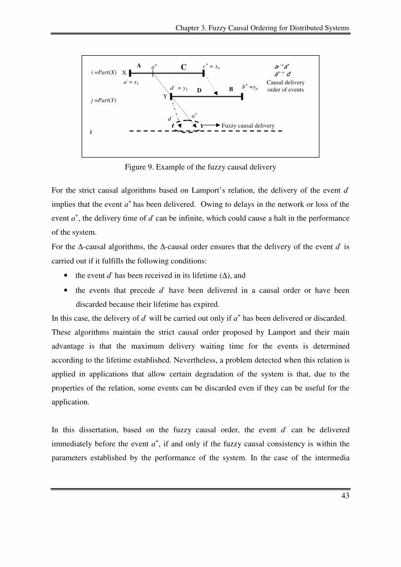
Chapter 3. Fuzzy Causal Ordering for Distributed Systems
43
Figure 9. Example of the fuzzy causal delivery
For the strict causal algorithms based on Lamport’s relation, the delivery of the event d-
implies that the event a+ has been delivered. Owing to delays in the network or loss of the
event a+, the delivery time of d- can be infinite, which could cause a halt in the performance
of the system.
For the ∆-causal algorithms, the ∆-causal order ensures that the delivery of the event d- is
carried out if it fulfills the following conditions:
• the event d- has been received in its lifetime (∆), and
• the events that precede d- have been delivered in a causal order or have been
discarded because their lifetime has expired.
In this case, the delivery of d- will be carried out only if a+ has been delivered or discarded.
These algorithms maintain the strict causal order proposed by Lamport and their main
advantage is that the maximum delivery waiting time for the events is determined
according to the lifetime established. Nevertheless, a problem detected when this relation is
applied in applications that allow certain degradation of the system is that, due to the
properties of the relation, some events can be discarded even if they can be useful for the
application.
In this dissertation, based on the fuzzy causal order, the event d- can be delivered
immediately before the event a+, if and only if the fuzzy causal consistency is within the
parameters established by the performance of the system. In the case of the intermedia
X
Y
a-→a+
a+→ d-
c-
a+
a- = x1 d - = y1 D
c+ = xn
b+ =yp
A C
B
a+
Causal delivery order of events
i =Part(X) j =Part(Y)
d -
Fuzzy causal delivery
k
a+
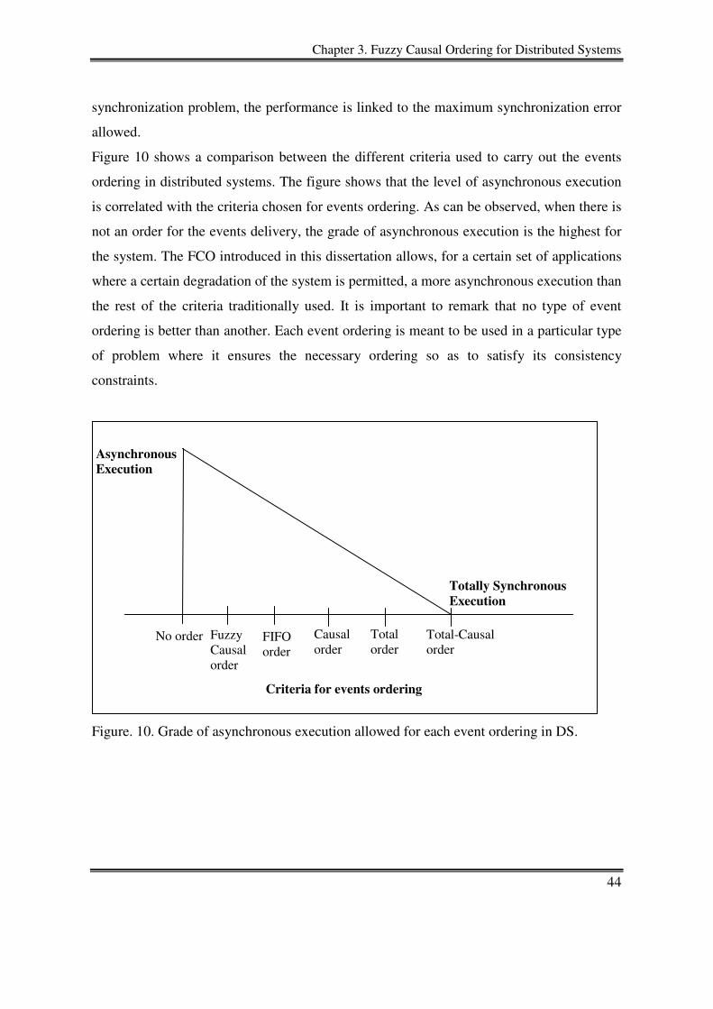
Chapter 3. Fuzzy Causal Ordering for Distributed Systems
44
synchronization problem, the performance is linked to the maximum synchronization error
allowed.
Figure 10 shows a comparison between the different criteria used to carry out the events
ordering in distributed systems. The figure shows that the level of asynchronous execution
is correlated with the criteria chosen for events ordering. As can be observed, when there is
not an order for the events delivery, the grade of asynchronous execution is the highest for
the system. The FCO introduced in this dissertation allows, for a certain set of applications
where a certain degradation of the system is permitted, a more asynchronous execution than
the rest of the criteria traditionally used. It is important to remark that no type of event
ordering is better than another. Each event ordering is meant to be used in a particular type
of problem where it ensures the necessary ordering so as to satisfy its consistency
constraints.
Figure. 10. Grade of asynchronous execution allowed for each event ordering in DS.
No order Causal order
Total order
Total-Causal order
Fuzzy Causal order
Totally Synchronous
Execution
Criteria for events ordering
FIFO order
Asynchronous
Execution
45
Chapter 4
“Get a good idea and stay with it. Dog it, and work at it until it's done right.”
Walt Disney(1901-1966)
Synchronization Model and Fuzzy
Control for Multimedia Systems
4.1 Introduction
In this chapter presents the theoretical aspects needed to implement the distributed
multimedia synchronization mechanism, which will be presented in Chapter 5. The
mechanism is composed of four main components, see figure 11. The first component is the
multimedia synchronization model, which is an extension of the model proposed by
Pomares et. al in [31]. The extension establishes synchronization periods from
synchronization points, which are identified by using the endpoints of the intervals. The
second component is the component of input variables, which includes the main variables
used by the fuzzy causal consistency and the fuzzy control system. The third is the fuzzy
causal component, which includes the FCR and the FCC applying them to the multimedia
synchronization problem. The last component is the fuzzy control system, which carries out
the multimedia synchronization for distributed system, adjusting the delivery time of the
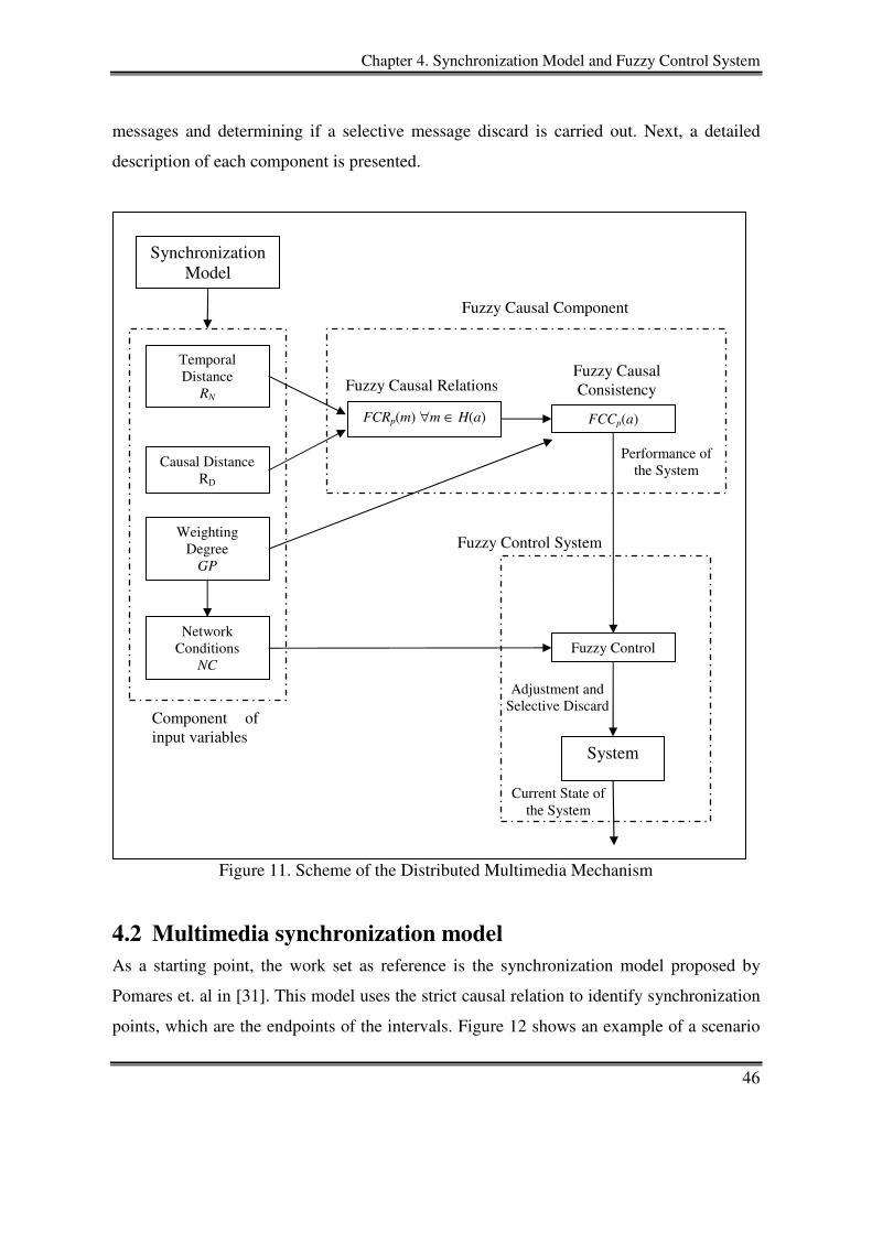
Chapter 4. Synchronization Model and Fuzzy Control System
46
messages and determining if a selective message discard is carried out. Next, a detailed
description of each component is presented.
Figure 11. Scheme of the Distributed Multimedia Mechanism
4.2 Multimedia synchronization model
As a starting point, the work set as reference is the synchronization model proposed by
Pomares et. al in [31]. This model uses the strict causal relation to identify synchronization
points, which are the endpoints of the intervals. Figure 12 shows an example of a scenario
Temporal Distance
RN
Causal Distance RD
FCRp(m) ∀m ∈ H(a) FCCp(a)
Fuzzy Control Network
Conditions NC
System
Component of input variables
Current State of the System
Adjustment and Selective Discard
Weighting Degree
GP
Fuzzy Causal Relations Fuzzy Causal Consistency
Synchronization Model
Fuzzy Causal Component
Fuzzy Control System
Performance of the System
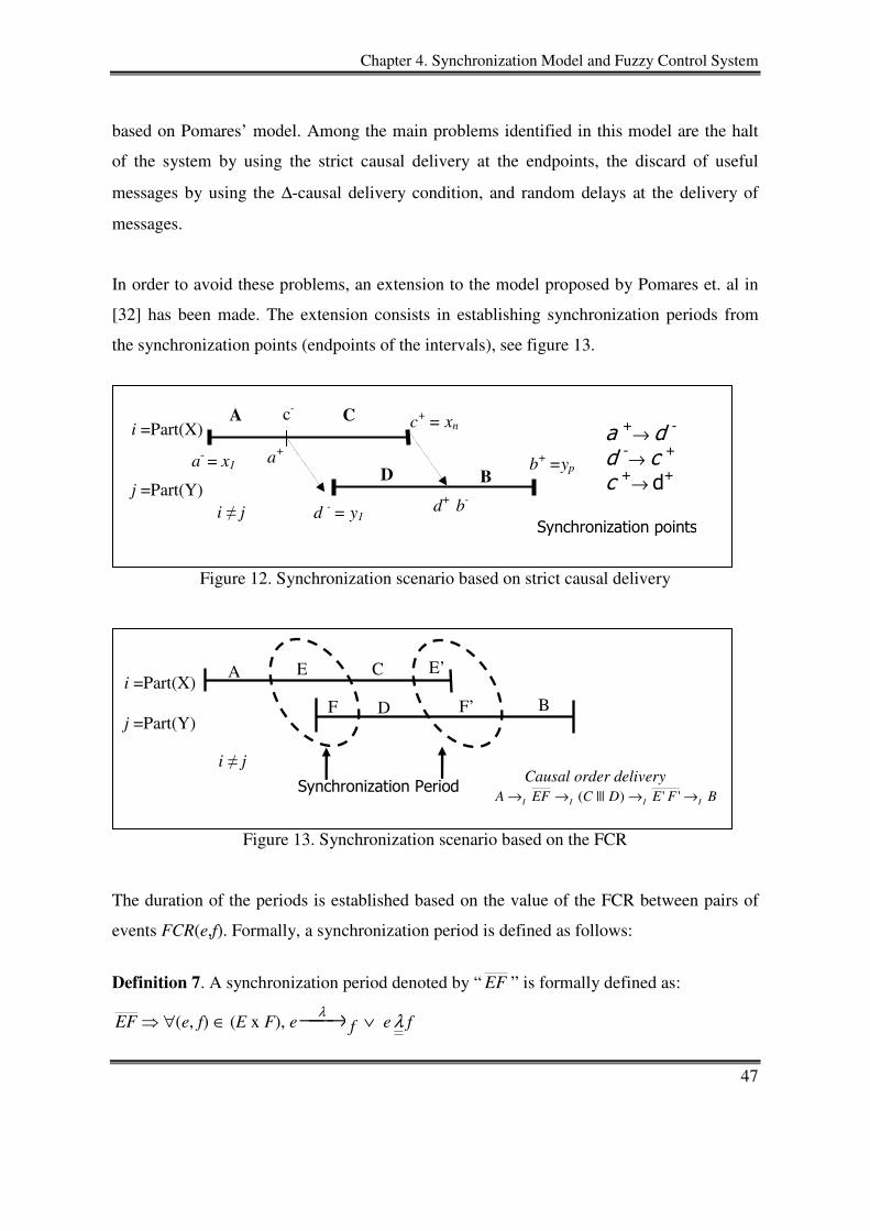
Chapter 4. Synchronization Model and Fuzzy Control System
47
based on Pomares’ model. Among the main problems identified in this model are the halt
of the system by using the strict causal delivery at the endpoints, the discard of useful
messages by using the ∆-causal delivery condition, and random delays at the delivery of
messages.
In order to avoid these problems, an extension to the model proposed by Pomares et. al in
[32] has been made. The extension consists in establishing synchronization periods from
the synchronization points (endpoints of the intervals), see figure 13.
Figure 12. Synchronization scenario based on strict causal delivery
Figure 13. Synchronization scenario based on the FCR
The duration of the periods is established based on the value of the FCR between pairs of
events FCR(e,f). Formally, a synchronization period is defined as follows:
Definition 7. A synchronization period denoted by “ EF ” is formally defined as:
EF ⇒ ∀(e, f) ∈ (E x F), e →λ f ∨ e λ f
i ≠ j
i =Part(X) j =Part(Y)
Synchronization Period
E’
F
A
B F’
E C
D
Causal order delivery BFEDCEFA IIII →→→→ '')|||(
a +→ d -
d -→ c +
c +→ d+
Synchronization points
D b+ =yp
c-
C
B
A
a+
c+ = xn
d+ b-
i =Part(X) j =Part(Y)
a- = x1
d - = y1 i ≠ j
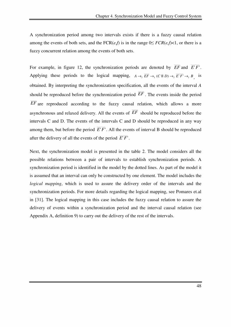
Chapter 4. Synchronization Model and Fuzzy Control System
48
A synchronization period among two intervals exists if there is a fuzzy causal relation
among the events of both sets, and the FCR(e,f) is in the range 0≤ FCR(e,f)<1, or there is a
fuzzy concurrent relation among the events of both sets.
For example, in figure 12, the synchronization periods are denoted by EF and ''FE .
Applying these periods to the logical mapping, BFEDCEFA IIII →→→→ '')|||( , is
obtained. By interpreting the synchronization specification, all the events of the interval A
should be reproduced before the synchronization period EF . The events inside the period
EF are reproduced according to the fuzzy causal relation, which allows a more
asynchronous and relaxed delivery. All the events of EF should be reproduced before the
intervals C and D. The events of the intervals C and D should be reproduced in any way
among them, but before the period ''FE . All the events of interval B should be reproduced
after the delivery of all the events of the period ''FE .
Next, the synchronization model is presented in the table 2. The model considers all the
possible relations between a pair of intervals to establish synchronization periods. A
synchronization period is identified in the model by the dotted lines. As part of the model it
is assumed that an interval can only be constructed by one element. The model includes the
logical mapping, which is used to assure the delivery order of the intervals and the
synchronization periods. For more details regarding the logical mapping, see Pomares et.al
in [31]. The logical mapping in this case includes the fuzzy causal relation to assure the
delivery of events within a synchronization period and the interval causal relation (see
Appendix A, definition 9) to carry out the delivery of the rest of the intervals.
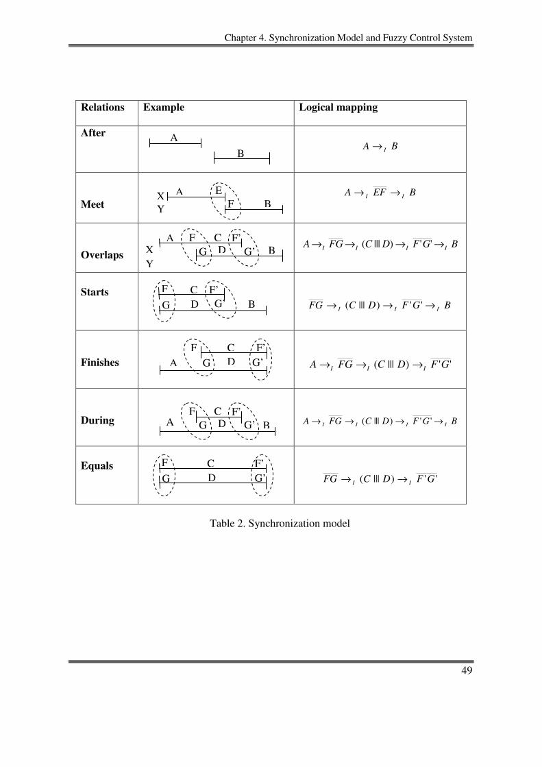
Chapter 4. Synchronization Model and Fuzzy Control System
49
Relations
Example Logical mapping
After
BA I→
Meet
BEFA II →→
Overlaps
BGFDCFGA IIII →→→→ '')|||(
Starts
BGFDCFG III →→→ '')|||(
Finishes
'')|||( GFDCFGA III →→→
During
BGFDCFGA IIII →→→→ '')|||(
Equals
'')|||( GFDCFG II →→
Table 2. Synchronization model
G C
G’ F’ F
D
G A F’ F C
D B G’
G A G’ F’ F C
D
G
C G’
F’ F
B D
G A
B G’ F’ F C
D
F E A
B X Y
B
A
X Y
Chapter 4. Synchronization Model and Fuzzy Control System
50
4.3 Component of input variables
Next, the main input variables used by the fuzzy causal component and the fuzzy control
system of the mechanism are presented in order to know the way in which they are
calculated.
4.3.1 Causal distance
The causal distance is used as an input variable of the membership function “RD” and it is
calculated at the reception of each message included in the synchronization period. The
Rd(m) measure the local causal distance between each causal message contained in the
causal history of m and last message received from each participant contained in its causal
history (last_messagep). The causal distance, defined by Lopez et. al in [22], between two
causally dependent messages is the greatest number of pairwise dependent messages sent
between them plus one. Formally, it is defined as follows:
Definition 8. The distance d(m,m’) is defined for any pair of messages m and m’ ∈ M
such that m→m’: d(m,m’) is the greatest integer n such that for some sequence of messages
(mi, i= 0...n) with m= m0 and m’=mn, we have mi↓mi+1 for all i=0…n-1.
In order to know the value of the causal distance among two events a collaboration with Dr.
Saúl Pomares Hernandez in the construction of an algorithm for the broadcast case for
distributed systems has been realized, this algorithm is shown in appendix B.
4.3.2 Temporal distance
The temporal distance is used as an input variable of the membership function “RN” and it
is also calculated at the reception of each message inside the synchronization period. The
temporal distance between two events is calculated at their reception by any participant
without having a global reference of time. In other words, it can be measured using only
independent local physical clocks for every participant. The ∆(m) measures the difference
in physical time between the arrival time of a message m and the arrival of the message m’
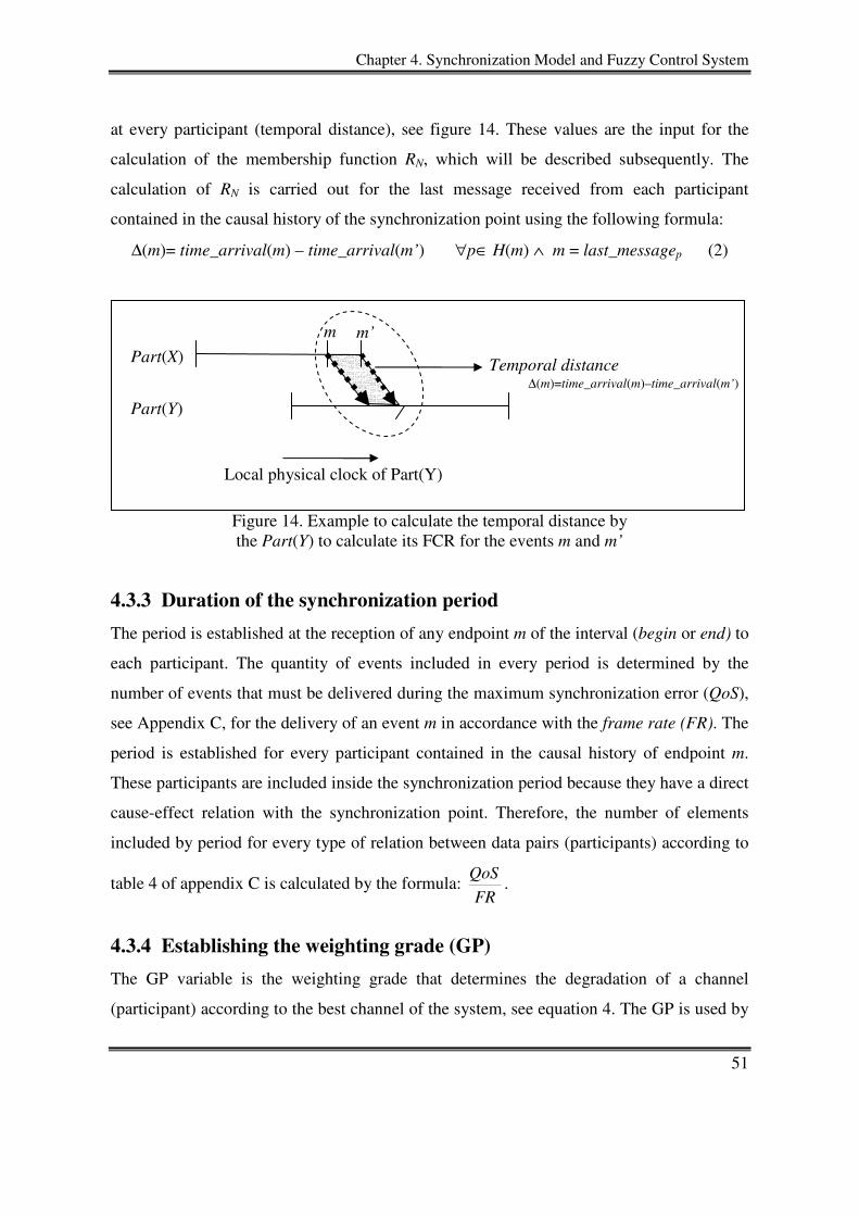
Chapter 4. Synchronization Model and Fuzzy Control System
51
at every participant (temporal distance), see figure 14. These values are the input for the
calculation of the membership function RN, which will be described subsequently. The
calculation of RN is carried out for the last message received from each participant
contained in the causal history of the synchronization point using the following formula:
∆(m)= time_arrival(m) – time_arrival(m’) ∀p∈ H(m) ∧ m = last_messagep (2)
Figure 14. Example to calculate the temporal distance by the Part(Y) to calculate its FCR for the events m and m’
4.3.3 Duration of the synchronization period
The period is established at the reception of any endpoint m of the interval (begin or end) to
each participant. The quantity of events included in every period is determined by the
number of events that must be delivered during the maximum synchronization error (QoS),
see Appendix C, for the delivery of an event m in accordance with the frame rate (FR). The
period is established for every participant contained in the causal history of endpoint m.
These participants are included inside the synchronization period because they have a direct
cause-effect relation with the synchronization point. Therefore, the number of elements
included by period for every type of relation between data pairs (participants) according to
table 4 of appendix C is calculated by the formula: FR
QoS.
4.3.4 Establishing the weighting grade (GP)
The GP variable is the weighting grade that determines the degradation of a channel
(participant) according to the best channel of the system, see equation 4. The GP is used by
Part(X)
Part(Y)
m m’
Local physical clock of Part(Y)
Temporal distance ∆(m)=time_arrival(m)–time_arrival(m’)
Chapter 4. Synchronization Model and Fuzzy Control System
52
the formulas that determine the network condition and the fuzzy causal consistency as an
input variable. This variable is obtained without a global reference of the system. In this
case only the partial view of the system to each participant is used. The variable GPi
establishes the weight that the channel i has in a certain time in order to calculate the
synchronization error with regard to the network conditions. With the GP, several problems
that arise when the messages are sent across the network have been considered. Such
problems include: traffic congestion, changes in the routing of the messages, which
increase the amount of time of the RTT, loss of messages, and message delivery delays.
(4)
In order to calculate the GP for the messages causally related to a, the channel with the best
network conditions, Bchannel, must first be chosen. This channel is chosen using the
following formula:
(5)
Once the BChannel is determined, the degradation of each channel with regard to the best
channel chosen is calculated by equation 4.
The mean of the variables used in equations 4 and 5 is the following:
• RTT is the Round trip time of a message.
• Jitter is the fluctuation of end to end of a message with the next message inside the
same stream.
• PP is the number of lost messages in a synchronization period.
• n is the number of channels (participants) which are causally related to the event a.
( )[ ]iiini PPjitterRTTBChannel ++= =1min
( )
++=
BChannel
PPjitterRTTGP iii
i
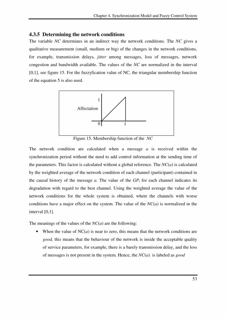
Chapter 4. Synchronization Model and Fuzzy Control System
53
4.3.5 Determining the network conditions
The variable NC determines in an indirect way the network conditions. The NC gives a
qualitative measurement (small, medium or big) of the changes in the network conditions,
for example, transmission delays, jitter among messages, loss of messages, network
congestion and bandwidth available. The values of the NC are normalized in the interval
[0,1], see figure 15. For the fuzzyfication value of NC, the triangular membership function
of the equation 5 is also used.
Figure 15. Membership function of the NC
The network condition are calculated when a message a is received within the
synchronization period without the need to add control information at the sending time of
the parameters. This factor is calculated without a global reference. The NC(a) is calculated
by the weighted average of the network condition of each channel (participant) contained in
the causal history of the message a. The value of the GPi for each channel indicates its
degradation with regard to the best channel. Using the weighted average the value of the
network conditions for the whole system is obtained, where the channels with worse
conditions have a major effect on the system. The value of the NC(a) is normalized in the
interval [0,1].
The meanings of the values of the NC(a) are the following:
• When the value of NC(a) is near to zero, this means that the network conditions are
good, this means that the behaviour of the network is inside the acceptable quality
of service parameters, for example, there is a barely transmission delay, and the loss
of messages is not present in the system. Hence, the NC(a) is labeled as good
Affectation
1
0
1
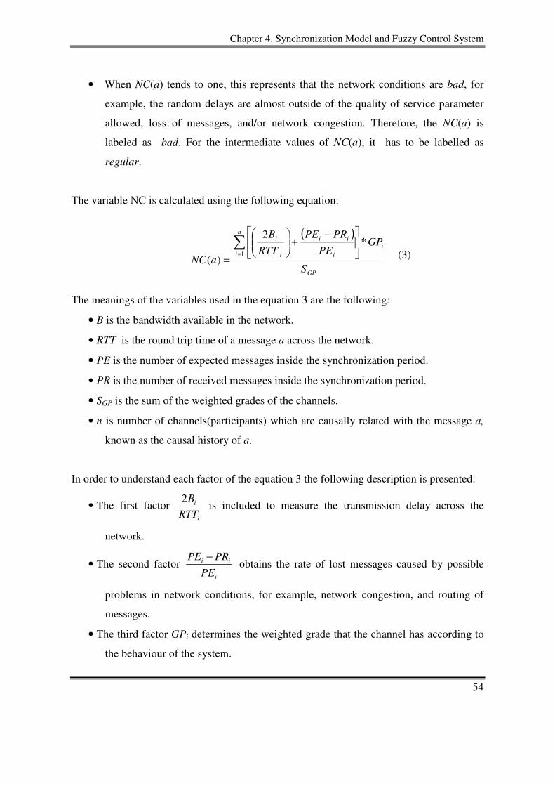
Chapter 4. Synchronization Model and Fuzzy Control System
54
• When NC(a) tends to one, this represents that the network conditions are bad, for
example, the random delays are almost outside of the quality of service parameter
allowed, loss of messages, and/or network congestion. Therefore, the NC(a) is
labeled as bad. For the intermediate values of NC(a), it has to be labelled as
regular.
The variable NC is calculated using the following equation:
(3)
The meanings of the variables used in the equation 3 are the following:
• B is the bandwidth available in the network.
• RTT is the round trip time of a message a across the network.
• PE is the number of expected messages inside the synchronization period.
• PR is the number of received messages inside the synchronization period.
• SGP is the sum of the weighted grades of the channels.
• n is number of channels(participants) which are causally related with the message a,
known as the causal history of a.
In order to understand each factor of the equation 3 the following description is presented:
• The first factor i
i
RTT
B2 is included to measure the transmission delay across the
network.
• The second factor i
ii
PE
PRPE − obtains the rate of lost messages caused by possible
problems in network conditions, for example, network congestion, and routing of
messages.
• The third factor GPi determines the weighted grade that the channel has according to
the behaviour of the system.
( )
GP
n
ii
i
ii
i
i
S
GPPE
PRPE
RTT
B
aNC
∑=
−+
=1
*2
)(
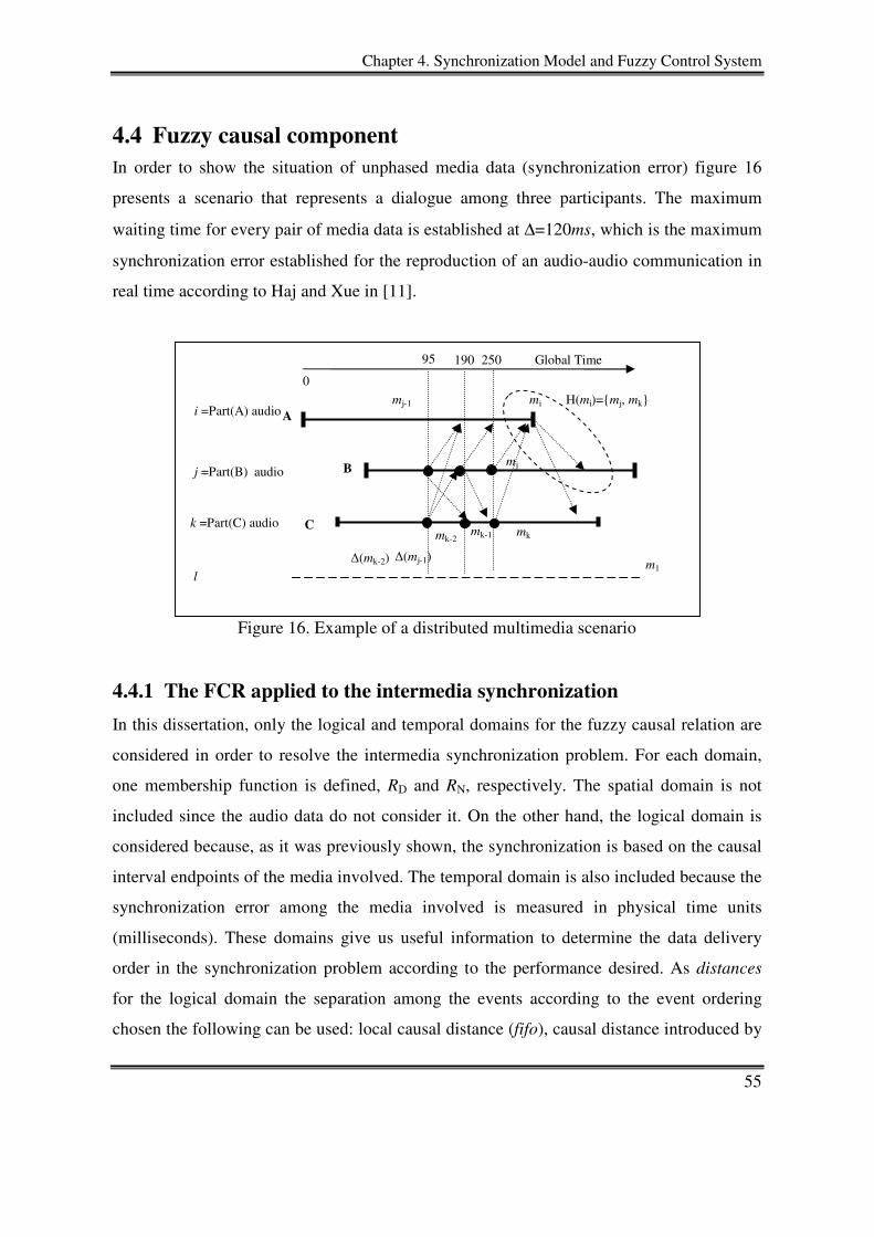
Chapter 4. Synchronization Model and Fuzzy Control System
55
4.4 Fuzzy causal component
In order to show the situation of unphased media data (synchronization error) figure 16
presents a scenario that represents a dialogue among three participants. The maximum
waiting time for every pair of media data is established at ∆=120ms, which is the maximum
synchronization error established for the reproduction of an audio-audio communication in
real time according to Haj and Xue in [11].
Figure 16. Example of a distributed multimedia scenario
4.4.1 The FCR applied to the intermedia synchronization
In this dissertation, only the logical and temporal domains for the fuzzy causal relation are
considered in order to resolve the intermedia synchronization problem. For each domain,
one membership function is defined, RD and RN, respectively. The spatial domain is not
included since the audio data do not consider it. On the other hand, the logical domain is
considered because, as it was previously shown, the synchronization is based on the causal
interval endpoints of the media involved. The temporal domain is also included because the
synchronization error among the media involved is measured in physical time units
(milliseconds). These domains give us useful information to determine the data delivery
order in the synchronization problem according to the performance desired. As distances
for the logical domain the separation among the events according to the event ordering
chosen the following can be used: local causal distance (fifo), causal distance introduced by
C
i =Part(A) audio j =Part(B) audio
k =Part(C) audio
A
B
∆(mk-2)
Global Time 95
0
190 250
mi H(mi)={mj, mk}
l m1
mk-2 mk-1 mk
mj-1
mj
∆(mj-1)
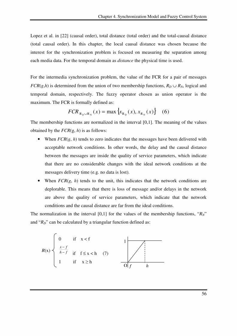
Chapter 4. Synchronization Model and Fuzzy Control System
56
Lopez et al. in [22] (causal order), total distance (total order) and the total-causal distance
(total causal order). In this chapter, the local causal distance was chosen because the
interest for the synchronization problem is focused on measuring the separation among
each media data. For the temporal domain as distance the physical time is used.
For the intermedia synchronization problem, the value of the FCR for a pair of messages
FCR(g,h) is determined from the union of two membership functions, RD ∪ RN, logical and
temporal domain, respectively. The fuzzy operator chosen as union operator is the
maximum. The FCR is formally defined as:
{ } )6()(),(max)(NDND RRRR xxxxxFCR =∪
The membership functions are normalized in the interval [0,1]. The meaning of the values
obtained by the FCR(g, h) is as follows:
• When FCR(g, h) tends to zero indicates that the messages have been delivered with
acceptable network conditions. In other words, the delay and the causal distance
between the messages are inside the quality of service parameters, which indicate
that there are no considerable changes with the ideal network conditions at the
messages delivery time (e.g. no data is lost).
• When FCR(g, h) tends to the unit, this indicates that the network conditions are
deplorable. This means that there is loss of message and/or delays in the network
are above the quality of service parameters, which indicate that the network
conditions and the causal distance are far from the ideal conditions.
The normalization in the interval [0,1] for the values of the membership functions, “RN”
and “RD” can be calculated by a triangular function defined as:
0 if x < f
fh
fx
−−
if f ≤ x < h (7)
1 if x ≥ h
R(x)
O f h
1
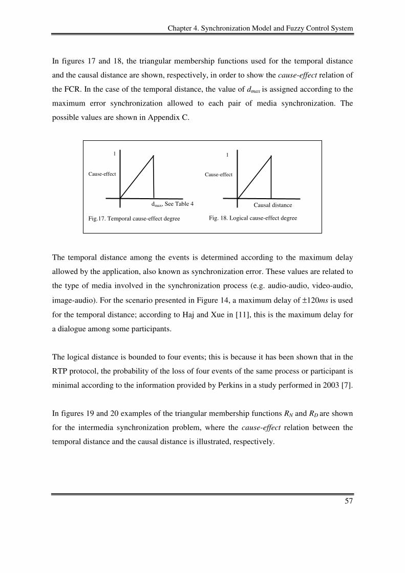
Chapter 4. Synchronization Model and Fuzzy Control System
57
In figures 17 and 18, the triangular membership functions used for the temporal distance
and the causal distance are shown, respectively, in order to show the cause-effect relation of
the FCR. In the case of the temporal distance, the value of dmax is assigned according to the
maximum error synchronization allowed to each pair of media synchronization. The
possible values are shown in Appendix C.
The temporal distance among the events is determined according to the maximum delay
allowed by the application, also known as synchronization error. These values are related to
the type of media involved in the synchronization process (e.g. audio-audio, video-audio,
image-audio). For the scenario presented in Figure 14, a maximum delay of ±120ms is used
for the temporal distance; according to Haj and Xue in [11], this is the maximum delay for
a dialogue among some participants.
The logical distance is bounded to four events; this is because it has been shown that in the
RTP protocol, the probability of the loss of four events of the same process or participant is
minimal according to the information provided by Perkins in a study performed in 2003 [7].
In figures 19 and 20 examples of the triangular membership functions RN and RD are shown
for the intermedia synchronization problem, where the cause-effect relation between the
temporal distance and the causal distance is illustrated, respectively.
Fig.17. Temporal cause-effect degree
Cause-effect
dmax, See Table 4
Fig. 18. Logical cause-effect degree
Cause-effect
1 1
Causal distance
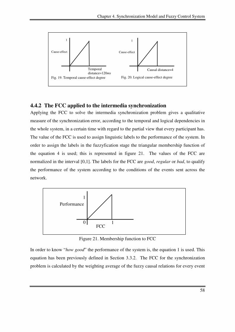
Chapter 4. Synchronization Model and Fuzzy Control System
58
4.4.2 The FCC applied to the intermedia synchronization
Applying the FCC to solve the intermedia synchronization problem gives a qualitative
measure of the synchronization error, according to the temporal and logical dependencies in
the whole system, in a certain time with regard to the partial view that every participant has.
The value of the FCC is used to assign linguistic labels to the performance of the system. In
order to assign the labels in the fuzzyfication stage the triangular membership function of
the equation 4 is used; this is represented in figure 21. The values of the FCC are
normalized in the interval [0,1]. The labels for the FCC are good, regular or bad, to qualify
the performance of the system according to the conditions of the events sent across the
network.
Figure 21. Membership function to FCC
In order to know “how good” the performance of the system is, the equation 1 is used. This
equation has been previously defined in Section 3.3.2. The FCC for the synchronization
problem is calculated by the weighting average of the fuzzy causal relations for every event
Performance
1
0
1
FCC
Fig. 19. Temporal cause-effect degree
Cause-effect
Temporal distance=120ms
Fig. 20. Logical cause-effect degree
Cause-effect
1 1
Causal distance=4
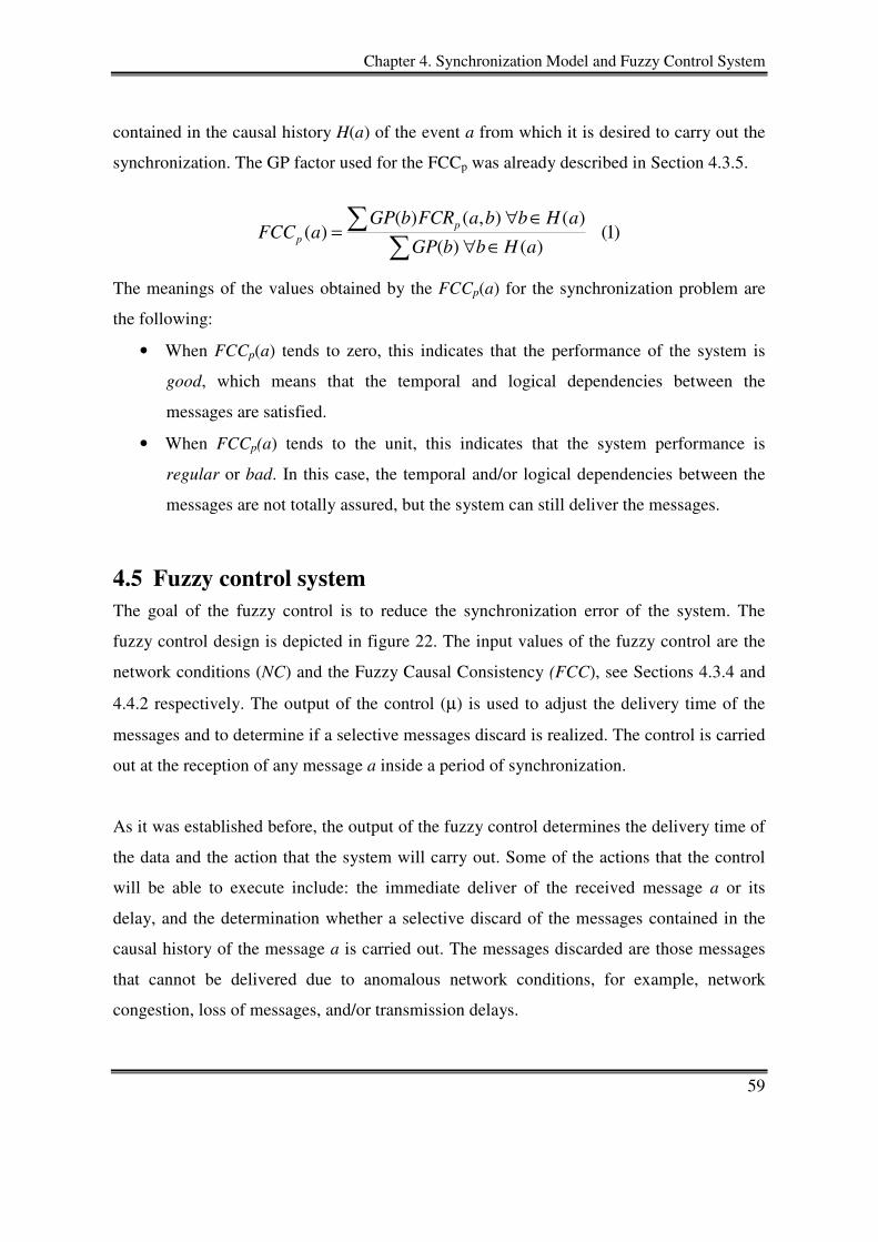
Chapter 4. Synchronization Model and Fuzzy Control System
59
contained in the causal history H(a) of the event a from which it is desired to carry out the
synchronization. The GP factor used for the FCCp was already described in Section 4.3.5.
)1()()(
)(),()()(
aHbbGP
aHbbaFCRbGPaFCC p
p ∈∀∈∀
=∑
∑
The meanings of the values obtained by the FCCp(a) for the synchronization problem are
the following:
• When FCCp(a) tends to zero, this indicates that the performance of the system is
good, which means that the temporal and logical dependencies between the
messages are satisfied.
• When FCCp(a) tends to the unit, this indicates that the system performance is
regular or bad. In this case, the temporal and/or logical dependencies between the
messages are not totally assured, but the system can still deliver the messages.
4.5 Fuzzy control system
The goal of the fuzzy control is to reduce the synchronization error of the system. The
fuzzy control design is depicted in figure 22. The input values of the fuzzy control are the
network conditions (NC) and the Fuzzy Causal Consistency (FCC), see Sections 4.3.4 and
4.4.2 respectively. The output of the control (µ) is used to adjust the delivery time of the
messages and to determine if a selective messages discard is realized. The control is carried
out at the reception of any message a inside a period of synchronization.
As it was established before, the output of the fuzzy control determines the delivery time of
the data and the action that the system will carry out. Some of the actions that the control
will be able to execute include: the immediate deliver of the received message a or its
delay, and the determination whether a selective discard of the messages contained in the
causal history of the message a is carried out. The messages discarded are those messages
that cannot be delivered due to anomalous network conditions, for example, network
congestion, loss of messages, and/or transmission delays.
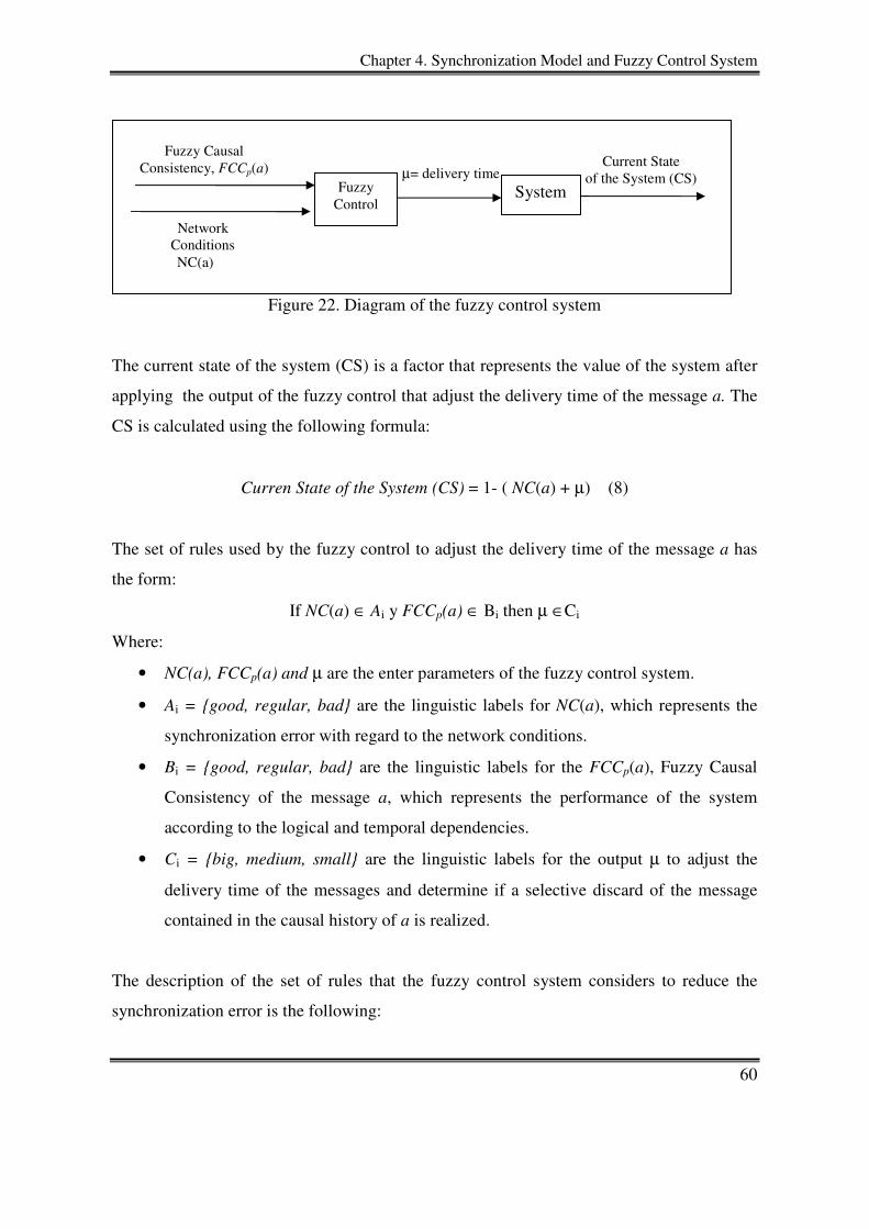
Chapter 4. Synchronization Model and Fuzzy Control System
60
Figure 22. Diagram of the fuzzy control system
The current state of the system (CS) is a factor that represents the value of the system after
applying the output of the fuzzy control that adjust the delivery time of the message a. The
CS is calculated using the following formula:
Curren State of the System (CS) = 1- ( NC(a) + µ) (8)
The set of rules used by the fuzzy control to adjust the delivery time of the message a has
the form:
If NC(a) ∈ Ai y FCCp(a) ∈ Bi then µ ∈Ci
Where:
• NC(a), FCCp(a) and µ are the enter parameters of the fuzzy control system.
• Ai = {good, regular, bad} are the linguistic labels for NC(a), which represents the
synchronization error with regard to the network conditions.
• Bi = {good, regular, bad} are the linguistic labels for the FCCp(a), Fuzzy Causal
Consistency of the message a, which represents the performance of the system
according to the logical and temporal dependencies.
• Ci = {big, medium, small} are the linguistic labels for the output µ to adjust the
delivery time of the messages and determine if a selective discard of the message
contained in the causal history of a is realized.
The description of the set of rules that the fuzzy control system considers to reduce the
synchronization error is the following:
Fuzzy Control
System µ= delivery time
Current State of the System (CS)
Fuzzy Causal Consistency, FCCp(a)
Network Conditions NC(a)
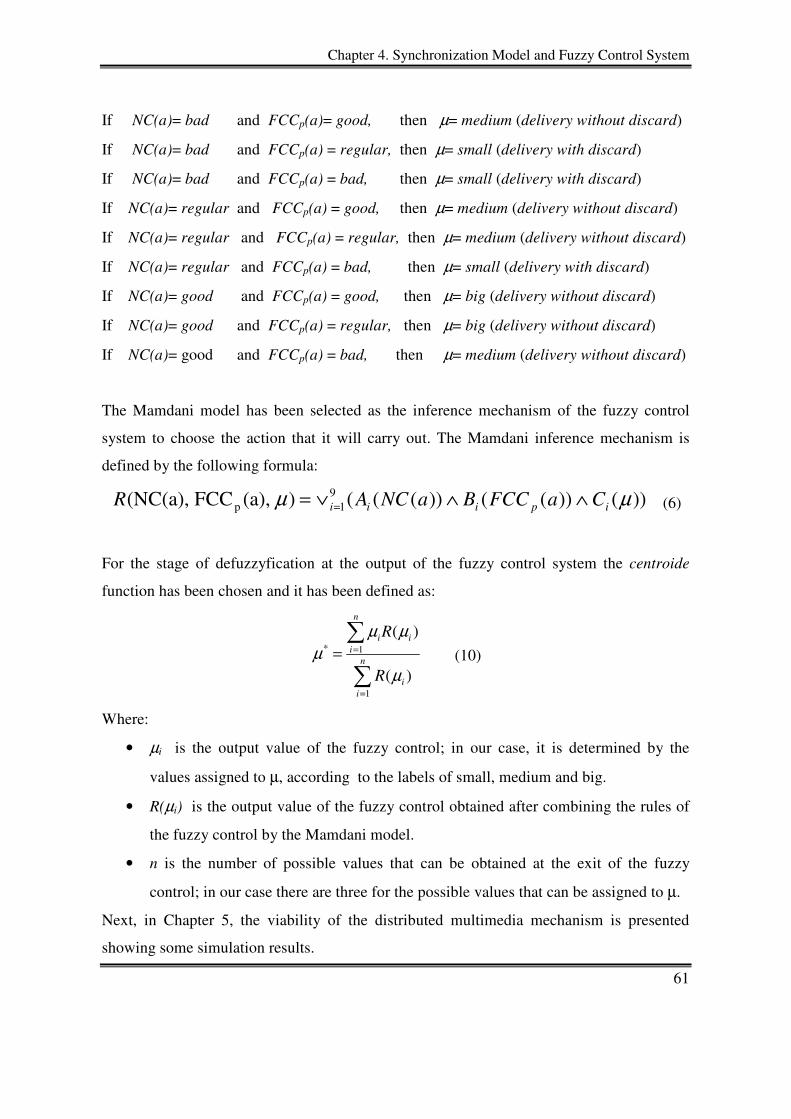
Chapter 4. Synchronization Model and Fuzzy Control System
61
If NC(a)= bad and FCCp(a)= good, then µ= medium (delivery without discard)
If NC(a)= bad and FCCp(a) = regular, then µ= small (delivery with discard)
If NC(a)= bad and FCCp(a) = bad, then µ= small (delivery with discard)
If NC(a)= regular and FCCp(a) = good, then µ= medium (delivery without discard)
If NC(a)= regular and FCCp(a) = regular, then µ= medium (delivery without discard)
If NC(a)= regular and FCCp(a) = bad, then µ= small (delivery with discard)
If NC(a)= good and FCCp(a) = good, then µ= big (delivery without discard)
If NC(a)= good and FCCp(a) = regular, then µ= big (delivery without discard)
If NC(a)= good and FCCp(a) = bad, then µ= medium (delivery without discard)
The Mamdani model has been selected as the inference mechanism of the fuzzy control
system to choose the action that it will carry out. The Mamdani inference mechanism is
defined by the following formula:
))())(())((( ) (a),FCC (NC(a), 91p µµ ipiii CaFCCBaNCAR ∧∧∨= = (6)
For the stage of defuzzyfication at the output of the fuzzy control system the centroide
function has been chosen and it has been defined as:
∑
∑
=
== n
ii
n
iii
R
R
1
1*
)(
)(
µ
µµµ (10)
Where:
• µi is the output value of the fuzzy control; in our case, it is determined by the
values assigned to µ, according to the labels of small, medium and big.
• R(µi) is the output value of the fuzzy control obtained after combining the rules of
the fuzzy control by the Mamdani model.
• n is the number of possible values that can be obtained at the exit of the fuzzy
control; in our case there are three for the possible values that can be assigned to µ.
Next, in Chapter 5, the viability of the distributed multimedia mechanism is presented
showing some simulation results.
62
Chapter 5
“Everything should be made as simple as possible, but not simpler.”
Albert Einstein(1879-1995)
Distributed Multimedia
Synchronization Mechanism
5.1 Introduction
The proposed mechanism to carry out the multimedia synchronization in a distributed
system in this chapter is presented. The mechanism main consists of an algorithm that
implement the four main components described in Chapter 4. In addition, a simulation of
the mechanism is presented in order to show its usefulness.
5.2 Distributed multimedia synchronization algorithm
First, the algorithm performs the logical mapping translation of a temporal scenario
according to the model presented in section 4.2 by establishing the synchronization periods
from the synchronizations points (interval endpoints). Secondly, the algorithm calculates
Chapter 5. Distributed Multimedia Synchronization Mechanism
63
the input variables used by the fuzzy control system and the fuzzy causal consistency. Next,
it determines the fuzzy causal relations and the fuzzy causal consistency to each message
received in the synchronization period. Finally, the algorithm carries out the fuzzy control
mechanism to establish the delivery time of the continuous media and takes corrective
actions in order to reduce the possible synchronization error among the media data. Next,
the formal codification of the algorithm is presented.
5.2.1 Algorithm codification
First, the main data structures used by the algorithm are presented. Later, the formal
codification of the algorithm is shown.
Main data structures
Structure of messages. Formally, a message m in the algorithm is a tuple m = (k, t, TP,
H(m), data), where:
• k is the identifier of sender k = Src(m).
• t = VT(p)[k] is the local process clock value with the identifier k when a causal
message m (begin, end or discrete) is sent. The value of t indicates the sequential
number labeled to the causal message.
• H(m) is the causal information of message m. It contains message identifiers (k,t),
which causally precede the causal message m. The information in H(m) ensures the
causal delivery of the message m. The H(m) structure is built before a causal
message is sent, and it is attached to the causal message. For fifo messages, the
structure H(m) is always H(m) = ∅.
• TP is the type of message (begin, end, or fifo,).
• data is the structure that carries the media data.
Causal data structures. There are four main causal structures: VT(p), VRCD(p), CI(p) and
last_fifo(p). The size of each structure is equal to the number of processes in the group.
• VT(p) is the vector time. Each process p has an element VT(p)[j] where j is a process
identifier. The VT(p)[j] represents the greatest number of messages that the
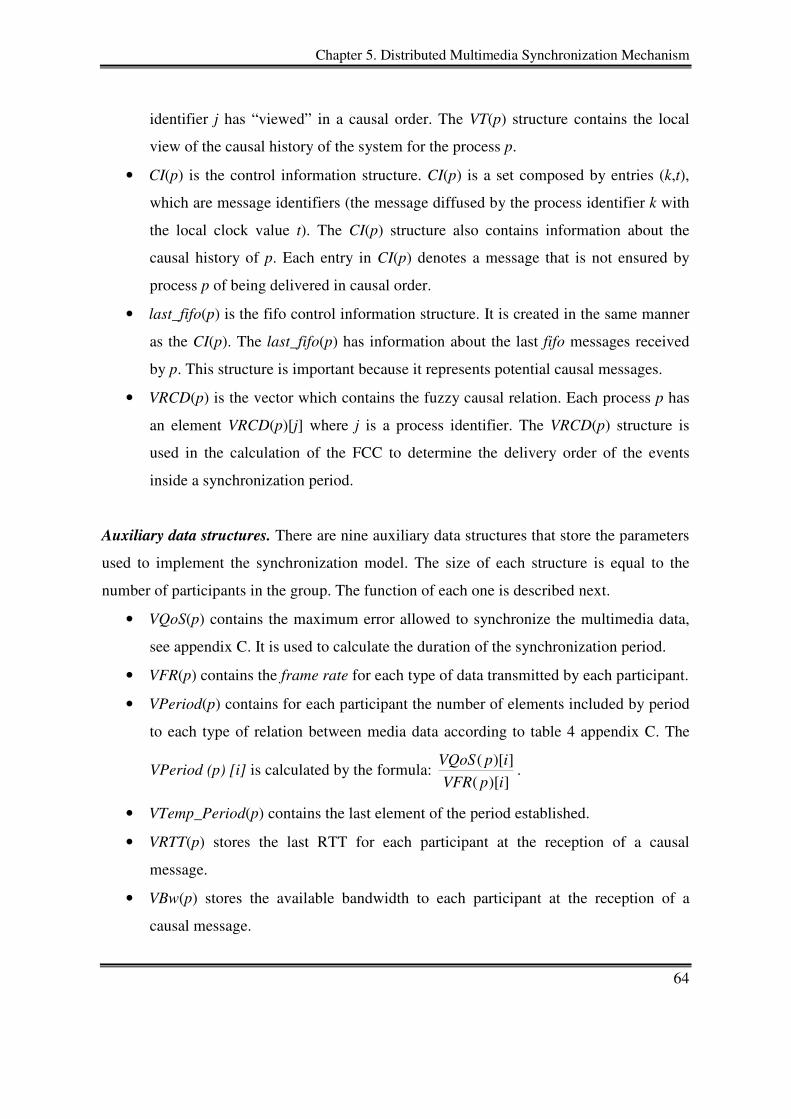
Chapter 5. Distributed Multimedia Synchronization Mechanism
64
identifier j has “viewed” in a causal order. The VT(p) structure contains the local
view of the causal history of the system for the process p.
• CI(p) is the control information structure. CI(p) is a set composed by entries (k,t),
which are message identifiers (the message diffused by the process identifier k with
the local clock value t). The CI(p) structure also contains information about the
causal history of p. Each entry in CI(p) denotes a message that is not ensured by
process p of being delivered in causal order.
• last_fifo(p) is the fifo control information structure. It is created in the same manner
as the CI(p). The last_fifo(p) has information about the last fifo messages received
by p. This structure is important because it represents potential causal messages.
• VRCD(p) is the vector which contains the fuzzy causal relation. Each process p has
an element VRCD(p)[j] where j is a process identifier. The VRCD(p) structure is
used in the calculation of the FCC to determine the delivery order of the events
inside a synchronization period.
Auxiliary data structures. There are nine auxiliary data structures that store the parameters
used to implement the synchronization model. The size of each structure is equal to the
number of participants in the group. The function of each one is described next.
• VQoS(p) contains the maximum error allowed to synchronize the multimedia data,
see appendix C. It is used to calculate the duration of the synchronization period.
• VFR(p) contains the frame rate for each type of data transmitted by each participant.
• VPeriod(p) contains for each participant the number of elements included by period
to each type of relation between media data according to table 4 appendix C. The
VPeriod (p) [i] is calculated by the formula: ])[(
])[(
ipVFR
ipVQoS.
• VTemp_Period(p) contains the last element of the period established.
• VRTT(p) stores the last RTT for each participant at the reception of a causal
message.
• VBw(p) stores the available bandwidth to each participant at the reception of a
causal message.
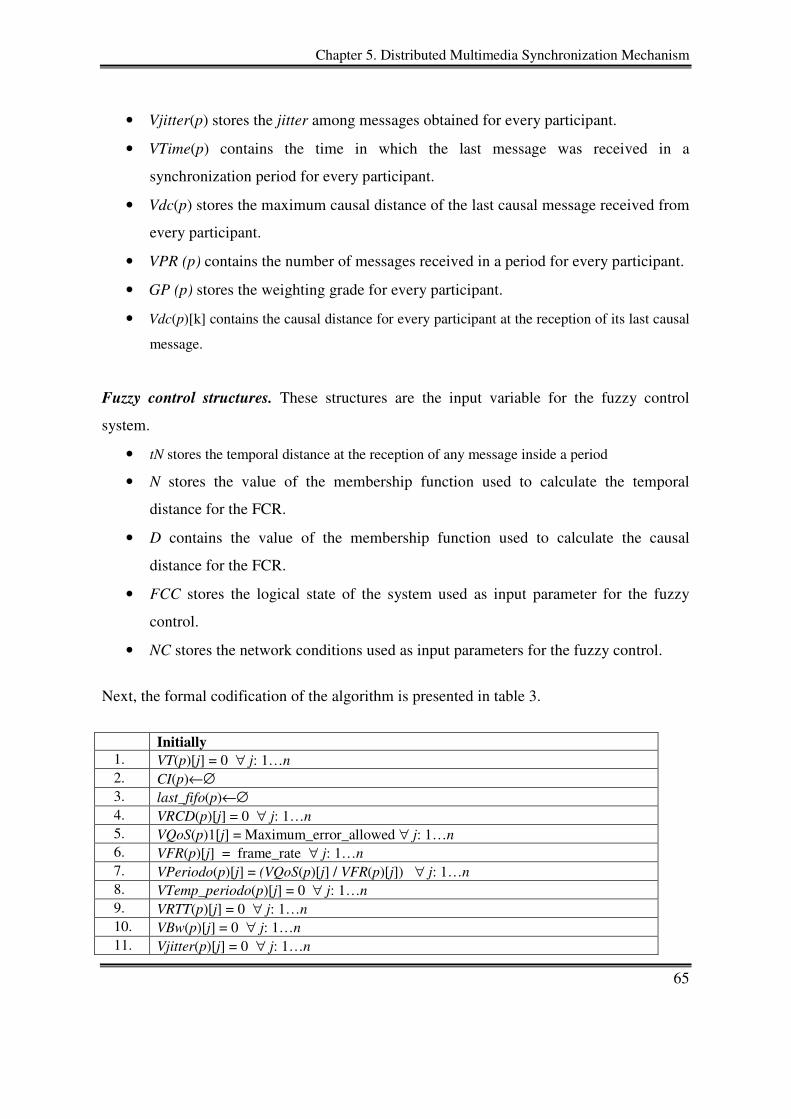
Chapter 5. Distributed Multimedia Synchronization Mechanism
65
• Vjitter(p) stores the jitter among messages obtained for every participant.
• VTime(p) contains the time in which the last message was received in a
synchronization period for every participant.
• Vdc(p) stores the maximum causal distance of the last causal message received from
every participant.
• VPR (p) contains the number of messages received in a period for every participant.
• GP (p) stores the weighting grade for every participant.
• Vdc(p)[k] contains the causal distance for every participant at the reception of its last causal
message.
Fuzzy control structures. These structures are the input variable for the fuzzy control
system.
• tN stores the temporal distance at the reception of any message inside a period
• N stores the value of the membership function used to calculate the temporal
distance for the FCR.
• D contains the value of the membership function used to calculate the causal
distance for the FCR.
• FCC stores the logical state of the system used as input parameter for the fuzzy
control.
• NC stores the network conditions used as input parameters for the fuzzy control.
Next, the formal codification of the algorithm is presented in table 3.
Initially
1. VT(p)[j] = 0 ∀ j: 1…n 2. CI(p)←∅ 3. last_fifo(p)←∅ 4. VRCD(p)[j] = 0 ∀ j: 1…n 5. VQoS(p)1[j] = Maximum_error_allowed ∀ j: 1…n 6. VFR(p)[j] = frame_rate ∀ j: 1…n 7. VPeriodo(p)[j] = (VQoS(p)[j] / VFR(p)[j]) ∀ j: 1…n 8. VTemp_periodo(p)[j] = 0 ∀ j: 1…n 9. VRTT(p)[j] = 0 ∀ j: 1…n 10. VBw(p)[j] = 0 ∀ j: 1…n 11. Vjitter(p)[j] = 0 ∀ j: 1…n
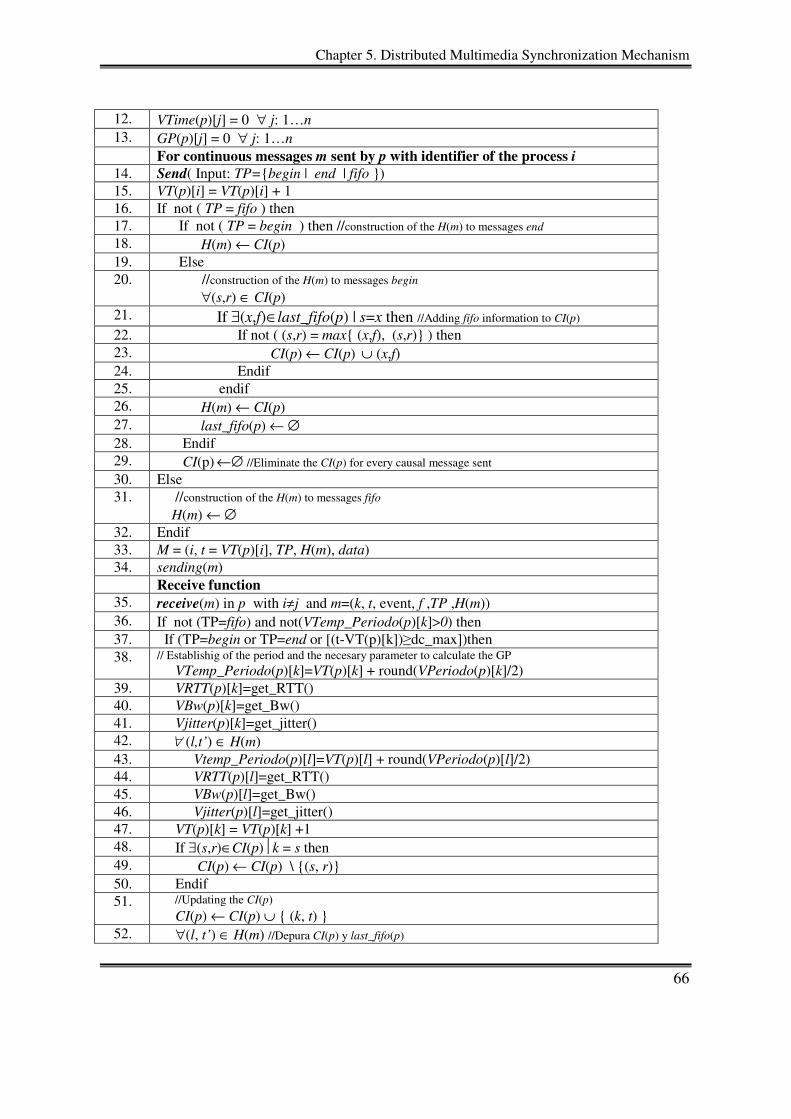
Chapter 5. Distributed Multimedia Synchronization Mechanism
66
12. VTime(p)[j] = 0 ∀ j: 1…n 13. GP(p)[j] = 0 ∀ j: 1…n
For continuous messages m sent by p with identifier of the process i
14. Send( Input: TP={begin | end | fifo }) 15. VT(p)[i] = VT(p)[i] + 1 16. If not ( TP = fifo ) then 17. If not ( TP = begin ) then //construction of the H(m) to messages end 18. H(m) ← CI(p)
19. Else 20. //construction of the H(m) to messages begin
∀(s,r) ∈ CI(p) 21. If ∃(x,f)∈last_fifo(p) | s=x then //Adding fifo information to CI(p) 22. If not ( (s,r) = max{ (x,f), (s,r)} ) then 23. CI(p) ← CI(p) ∪ (x,f) 24. Endif 25. endif 26. H(m) ← CI(p) 27. last_fifo(p) ← ∅ 28. Endif 29. CI(p) ←∅ //Eliminate the CI(p) for every causal message sent 30. Else 31. //construction of the H(m) to messages fifo
H(m) ← ∅
32. Endif 33. M = (i, t = VT(p)[i], TP, H(m), data) 34. sending(m)
Receive function
35. receive(m) in p with i≠j and m=(k, t, event, f ,TP ,H(m)) 36. If not (TP=fifo) and not(VTemp_Periodo(p)[k]>0) then 37. If (TP=begin or TP=end or [(t-VT(p)[k])≥dc_max])then 38. // Establishig of the period and the necesary parameter to calculate the GP
VTemp_Periodo(p)[k]=VT(p)[k] + round(VPeriodo(p)[k]/2) 39. VRTT(p)[k]=get_RTT() 40. VBw(p)[k]=get_Bw() 41. Vjitter(p)[k]=get_jitter() 42. ∀ (l,t’) ∈ H(m) 43. Vtemp_Periodo(p)[l]=VT(p)[l] + round(VPeriodo(p)[l]/2) 44. VRTT(p)[l]=get_RTT() 45. VBw(p)[l]=get_Bw() 46. Vjitter(p)[l]=get_jitter() 47. VT(p)[k] = VT(p)[k] +1 48. If ∃(s,r)∈CI(p)k = s then 49. CI(p) ← CI(p) \ {(s, r)} 50. Endif 51. //Updating the CI(p)
CI(p) ← CI(p) ∪ { (k, t) } 52. ∀(l, t’) ∈ H(m) //Depura CI(p) y last_fifo(p)
Chapter 5. Distributed Multimedia Synchronization Mechanism
67
53. If ∃ (s, r) ∈ CI(p) | l=s and r ≤ t’ then 54. CI(p) ← CI(p) \ (s, r) 55. Endif 56. If ∃ (x,f) ∈ last_fifo(p) | l=x and f ≤ t’ then 57. last_fifo(p) ← last_fifo(p) \ (x, f) 58. Endif 59. Else 60. // Cheking the range of the period
If (VTemp_Periodo(p)[k]<VT(p)[k]) 61. VTemp_Periodo(p)[k]=0 62. ∀ (l,t’) ∈ H(m) 63. If (VTemp_Periodo(p)[l] <VT(p)[l]) 64. VTemp_Periodo(p)[l]=0
65. End 66. // Reception and delivery of message inside the period
If (VTemp_Periodo(p)[k]>0) 67. tN =get_time(actual)-VTime(p)[k] 68. Vtime(p)[k]=get_time(actual) 69. d= t-VT(p)[k] 70. If TP=fifo 71. dc_max=d 72. Else 73. dc_max=0 74. ∀ (l,t’) ∈ H’(m) 75. If dc_max<d 76. dc_max=d 77. d=t’-VT(p)[l] 78. Endif 79. Vdc(p)[k]=dc_max 80. D= t-VT(p)[k] 81. N=[(tN)/( VQoS2(p)[k]) 82. D=[(Vdc(p)[k])/( Vd2(p)[k]) 83. // Calculate of the RCD
VRCD(p)[k]=max(N,D) 84. ∀ (l,t’) ∈ H(m) 85. GP(p)[l]=[VRTT(p)[l])+Vjitter(p)[l]]+((VPeriodo(p)[l]-VPR(p)[l]) 86. GP(p)[k]=[VRTT(p)[k])+Vjitter(p)[k]]+((VPeriodo(p)[k]-VPR(p)[k]) 87. BChannel=max(GP (p)[l] ∀ (l,t’) ∈ H’(m), GP(p)[k] ) 88. FCC=0 89. ∀ (l,t’) ∈ H(m) 90. FCC= FCC+(VRCD(p)[l]* VGP(p)[l]) 91. CS=CS+[((2*VBw(p)[l])/VRTT(p)[l])+((VPeriodo(p)[l]-
VPR(p)[l])/VPE(p)[l])]*(GP(p)[l]/BChannel) 92. FCC= FCC+(VRCD(p)[k]* VGP(p)[k]) 93. NC=NC+[((2*VBw(p)[k])/VRTT(p)[k])+((VPeriodo(p)[k]-
VPR(p)[k])/VPE(p)[k])]*(GP(p)[k]/BChannel) 94. //Calculate the fuzzy causal consistency
FCC= FCC/ ngp
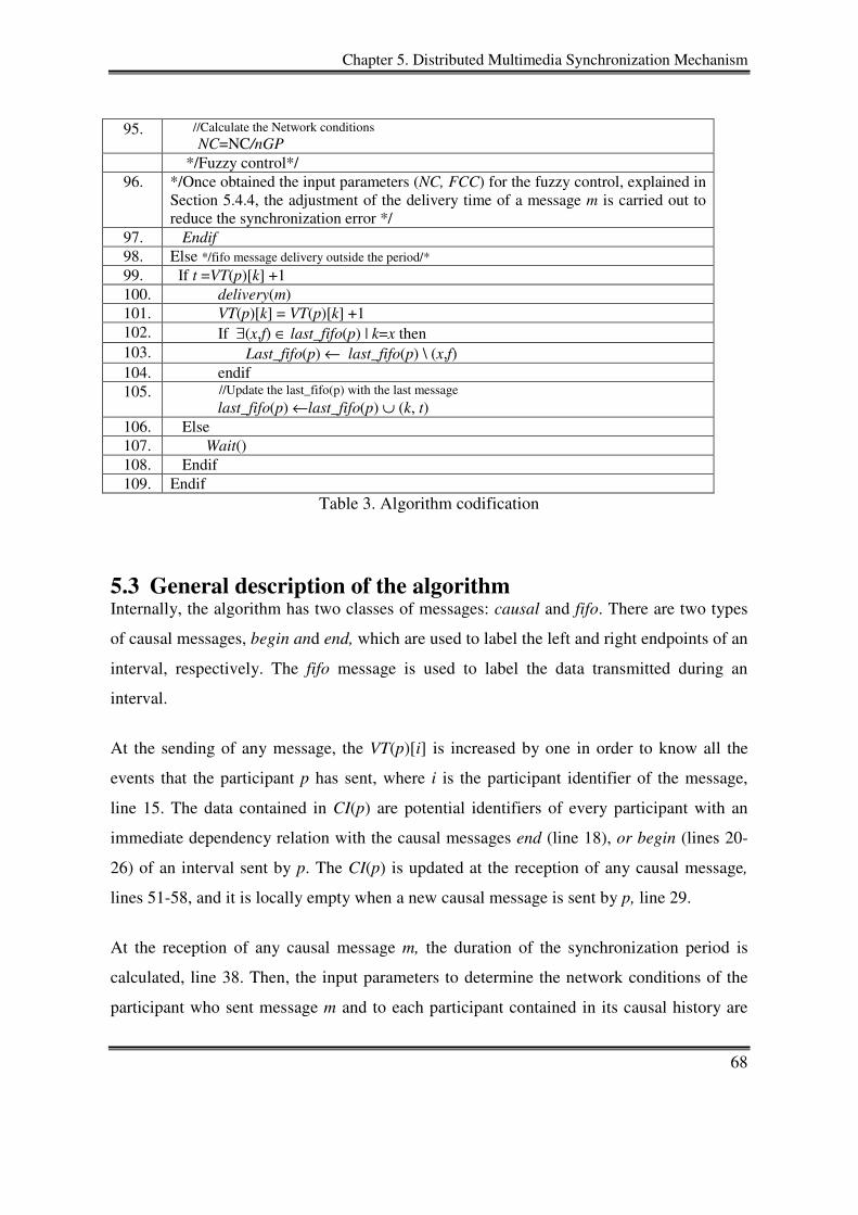
Chapter 5. Distributed Multimedia Synchronization Mechanism
68
95. //Calculate the Network conditions NC=NC/nGP
*/Fuzzy control*/ 96. */Once obtained the input parameters (NC, FCC) for the fuzzy control, explained in
Section 5.4.4, the adjustment of the delivery time of a message m is carried out to reduce the synchronization error */
97. Endif 98. Else */fifo message delivery outside the period/* 99. If t =VT(p)[k] +1 100. delivery(m) 101. VT(p)[k] = VT(p)[k] +1 102. If ∃(x,f) ∈ last_fifo(p) | k=x then 103. Last_fifo(p) ← last_fifo(p) \ (x,f) 104. endif 105. //Update the last_fifo(p) with the last message
last_fifo(p) ←last_fifo(p) ∪ (k, t) 106. Else 107. Wait() 108. Endif 109. Endif
Table 3. Algorithm codification
5.3 General description of the algorithm Internally, the algorithm has two classes of messages: causal and fifo. There are two types
of causal messages, begin and end, which are used to label the left and right endpoints of an
interval, respectively. The fifo message is used to label the data transmitted during an
interval.
At the sending of any message, the VT(p)[i] is increased by one in order to know all the
events that the participant p has sent, where i is the participant identifier of the message,
line 15. The data contained in CI(p) are potential identifiers of every participant with an
immediate dependency relation with the causal messages end (line 18), or begin (lines 20-
26) of an interval sent by p. The CI(p) is updated at the reception of any causal message,
lines 51-58, and it is locally empty when a new causal message is sent by p, line 29.
At the reception of any causal message m, the duration of the synchronization period is
calculated, line 38. Then, the input parameters to determine the network conditions of the
participant who sent message m and to each participant contained in its causal history are
Chapter 5. Distributed Multimedia Synchronization Mechanism
69
obtained: the RTT, the available bandwidth (Bw) and the jitter among messages, lines 38-
41.
For any message received during a synchronization period, the FCR is calculated. Then, in
order to establish the fuzzy causal relation among the messages, it is necessary to obtain the
temporal distance “RN” and the logical distance “RD” (causal distance), lines 70-77.
Later, the average weight (GP) is calculated according to the network parameters
previously obtained, lines 84-86.
Next, the fuzzy causal consistency and the network conditions are calculated, see lines 88-
95. These parameters are used as input variables for the fuzzy control in order to overcome
the synchronization error. Moreover, the control adjusts the delivery time of the message
determining if a selective discard of the messages contained in the causal history of m is
carried out, line 96.
When a fifo message is received outside of a synchronization period, the FIFO order of
delivery is verified. In addition, the information of the last message received by this
participant is updated, see lines 99-108.
5.4 Simulation This section presents the simulations of the synchronization mechanism. The input
variables used by the fuzzy control and the output of the control are described. The number
of tests developed was 100,000.
In order to illustrate the situation of unphased media data (synchronization error) a scenario
that consists of a group of four hosts is presented; three of them transmitting live media
data (W, X, and Y hosts), while the other function only serves as a Client (Host Z); see
Figure 13.
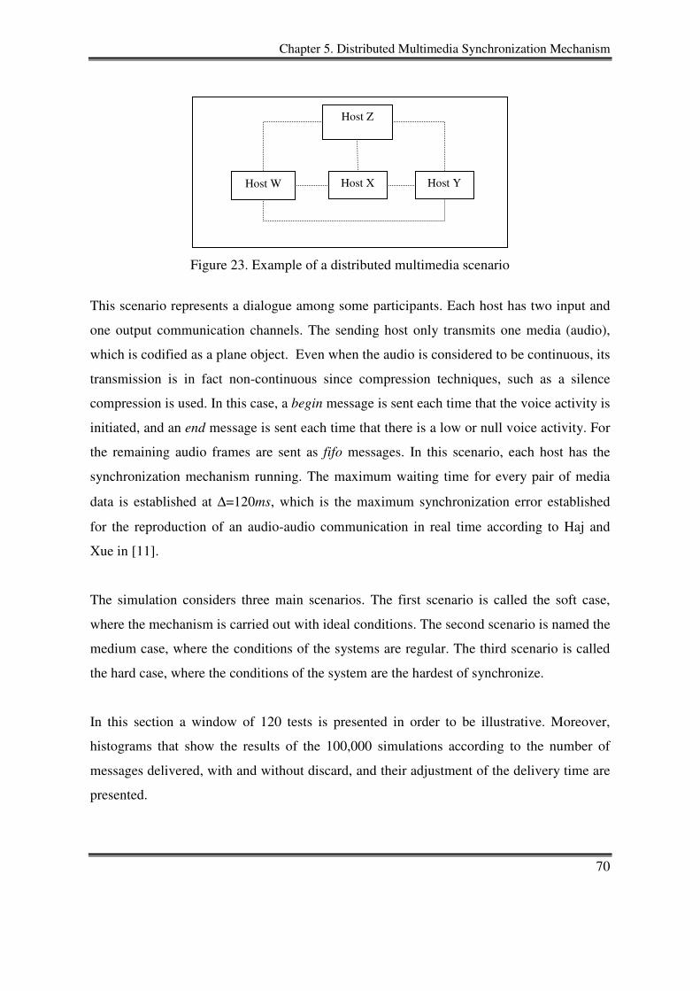
Chapter 5. Distributed Multimedia Synchronization Mechanism
70
Figure 23. Example of a distributed multimedia scenario
This scenario represents a dialogue among some participants. Each host has two input and
one output communication channels. The sending host only transmits one media (audio),
which is codified as a plane object. Even when the audio is considered to be continuous, its
transmission is in fact non-continuous since compression techniques, such as a silence
compression is used. In this case, a begin message is sent each time that the voice activity is
initiated, and an end message is sent each time that there is a low or null voice activity. For
the remaining audio frames are sent as fifo messages. In this scenario, each host has the
synchronization mechanism running. The maximum waiting time for every pair of media
data is established at ∆=120ms, which is the maximum synchronization error established
for the reproduction of an audio-audio communication in real time according to Haj and
Xue in [11].
The simulation considers three main scenarios. The first scenario is called the soft case,
where the mechanism is carried out with ideal conditions. The second scenario is named the
medium case, where the conditions of the systems are regular. The third scenario is called
the hard case, where the conditions of the system are the hardest of synchronize.
In this section a window of 120 tests is presented in order to be illustrative. Moreover,
histograms that show the results of the 100,000 simulations according to the number of
messages delivered, with and without discard, and their adjustment of the delivery time are
presented.
Host W Host X
Host Z
Host Y
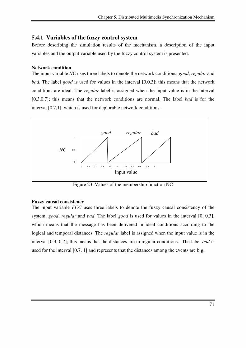
Chapter 5. Distributed Multimedia Synchronization Mechanism
71
5.4.1 Variables of the fuzzy control system
Before describing the simulation results of the mechanism, a description of the input
variables and the output variable used by the fuzzy control system is presented.
Network condition
The input variable NC uses three labels to denote the network conditions, good, regular and
bad. The label good is used for values in the interval [0,0.3]; this means that the network
conditions are ideal. The regular label is assigned when the input value is in the interval
[0.3,0.7]; this means that the network conditions are normal. The label bad is for the
interval [0.7,1], which is used for deplorable network conditions.
Figure 23. Values of the membership function NC
Fuzzy causal consistency
The input variable FCC uses three labels to denote the fuzzy causal consistency of the
system, good, regular and bad. The label good is used for values in the interval [0, 0.3],
which means that the message has been delivered in ideal conditions according to the
logical and temporal distances. The regular label is assigned when the input value is in the
interval [0.3, 0.7]; this means that the distances are in regular conditions. The label bad is
used for the interval [0.7, 1] and represents that the distances among the events are big.
0
0.5
1
0 0.1 0.2 0.3 0.4 0.5 0.6 0.7 0.8 0.9 1
good regular bad
NC
Input value
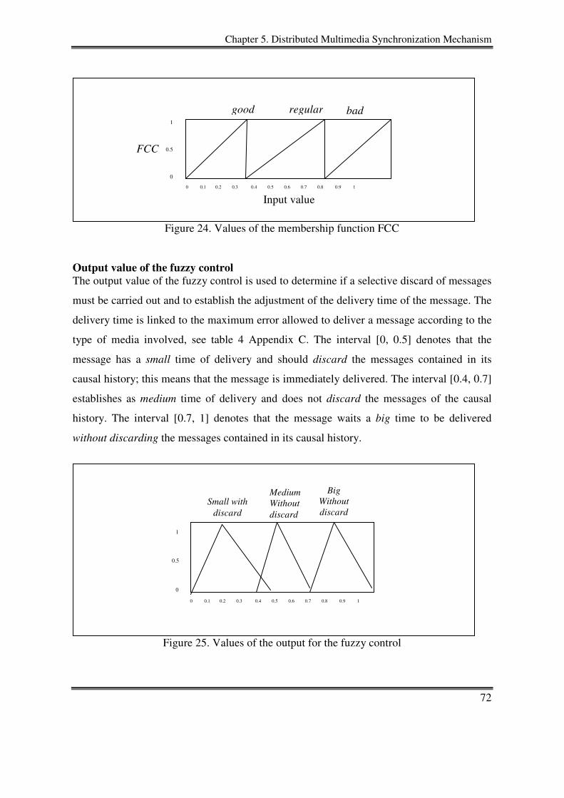
Chapter 5. Distributed Multimedia Synchronization Mechanism
72
Figure 24. Values of the membership function FCC
Output value of the fuzzy control
The output value of the fuzzy control is used to determine if a selective discard of messages
must be carried out and to establish the adjustment of the delivery time of the message. The
delivery time is linked to the maximum error allowed to deliver a message according to the
type of media involved, see table 4 Appendix C. The interval [0, 0.5] denotes that the
message has a small time of delivery and should discard the messages contained in its
causal history; this means that the message is immediately delivered. The interval [0.4, 0.7]
establishes as medium time of delivery and does not discard the messages of the causal
history. The interval [0.7, 1] denotes that the message waits a big time to be delivered
without discarding the messages contained in its causal history.
Figure 25. Values of the output for the fuzzy control
Small with discard
Medium Without discard
Big Without discard
0
0.5
1
0 0.1 0.2 0.3 0.4 0.5 0.6 0.7 0.8 0.9 1
0
0.5
1
0 0.1 0.2 0.3 0.4 0.5 0.6 0.7 0.8 0.9 1
good regular bad
FCC
Input value
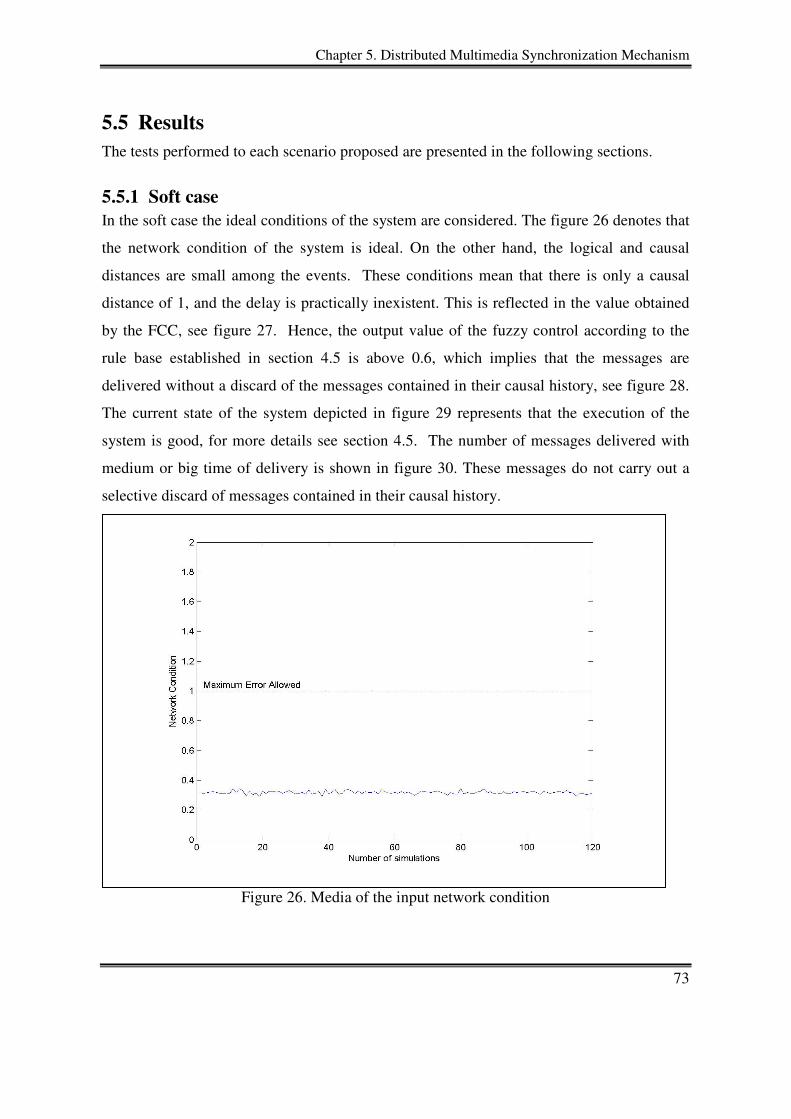
Chapter 5. Distributed Multimedia Synchronization Mechanism
73
5.5 Results
The tests performed to each scenario proposed are presented in the following sections.
5.5.1 Soft case
In the soft case the ideal conditions of the system are considered. The figure 26 denotes that
the network condition of the system is ideal. On the other hand, the logical and causal
distances are small among the events. These conditions mean that there is only a causal
distance of 1, and the delay is practically inexistent. This is reflected in the value obtained
by the FCC, see figure 27. Hence, the output value of the fuzzy control according to the
rule base established in section 4.5 is above 0.6, which implies that the messages are
delivered without a discard of the messages contained in their causal history, see figure 28.
The current state of the system depicted in figure 29 represents that the execution of the
system is good, for more details see section 4.5. The number of messages delivered with
medium or big time of delivery is shown in figure 30. These messages do not carry out a
selective discard of messages contained in their causal history.
Figure 26. Media of the input network condition
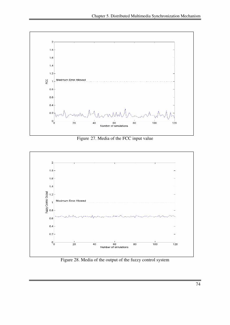
Chapter 5. Distributed Multimedia Synchronization Mechanism
74
Figure 27. Media of the FCC input value
Figure 28. Media of the output of the fuzzy control system
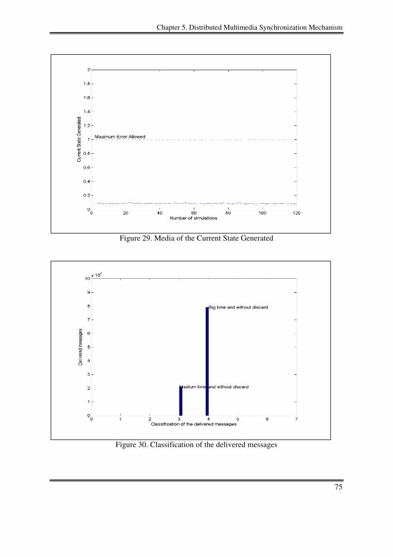
Chapter 5. Distributed Multimedia Synchronization Mechanism
75
Figure 29. Media of the Current State Generated
Figure 30. Classification of the delivered messages
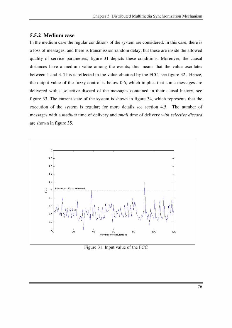
Chapter 5. Distributed Multimedia Synchronization Mechanism
76
5.5.2 Medium case
In the medium case the regular conditions of the system are considered. In this case, there is
a loss of messages, and there is transmission random delay; but these are inside the allowed
quality of service parameters; figure 31 depicts these conditions. Moreover, the causal
distances have a medium value among the events; this means that the value oscillates
between 1 and 3. This is reflected in the value obtained by the FCC, see figure 32. Hence,
the output value of the fuzzy control is below 0.6, which implies that some messages are
delivered with a selective discard of the messages contained in their causal history, see
figure 33. The current state of the system is shown in figure 34, which represents that the
execution of the system is regular; for more details see section 4.5. The number of
messages with a medium time of delivery and small time of delivery with selective discard
are shown in figure 35.
Figure 31. Input value of the FCC
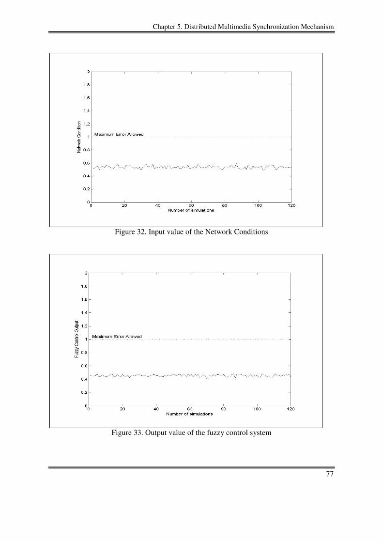
Chapter 5. Distributed Multimedia Synchronization Mechanism
77
Figure 32. Input value of the Network Conditions
Figure 33. Output value of the fuzzy control system
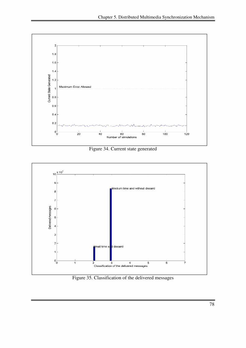
Chapter 5. Distributed Multimedia Synchronization Mechanism
78
Figure 34. Current state generated
Figure 35. Classification of the delivered messages
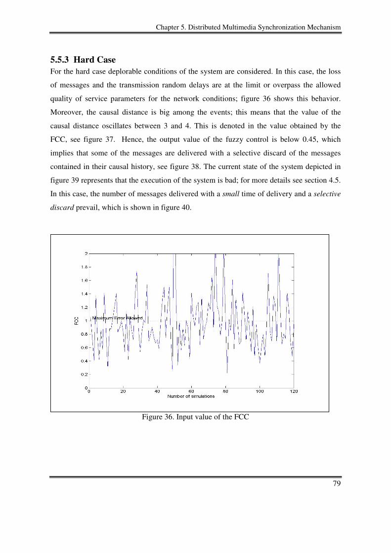
Chapter 5. Distributed Multimedia Synchronization Mechanism
79
5.5.3 Hard Case
For the hard case deplorable conditions of the system are considered. In this case, the loss
of messages and the transmission random delays are at the limit or overpass the allowed
quality of service parameters for the network conditions; figure 36 shows this behavior.
Moreover, the causal distance is big among the events; this means that the value of the
causal distance oscillates between 3 and 4. This is denoted in the value obtained by the
FCC, see figure 37. Hence, the output value of the fuzzy control is below 0.45, which
implies that some of the messages are delivered with a selective discard of the messages
contained in their causal history, see figure 38. The current state of the system depicted in
figure 39 represents that the execution of the system is bad; for more details see section 4.5.
In this case, the number of messages delivered with a small time of delivery and a selective
discard prevail, which is shown in figure 40.
Figure 36. Input value of the FCC
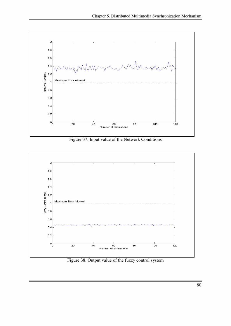
Chapter 5. Distributed Multimedia Synchronization Mechanism
80
Figure 37. Input value of the Network Conditions
Figure 38. Output value of the fuzzy control system
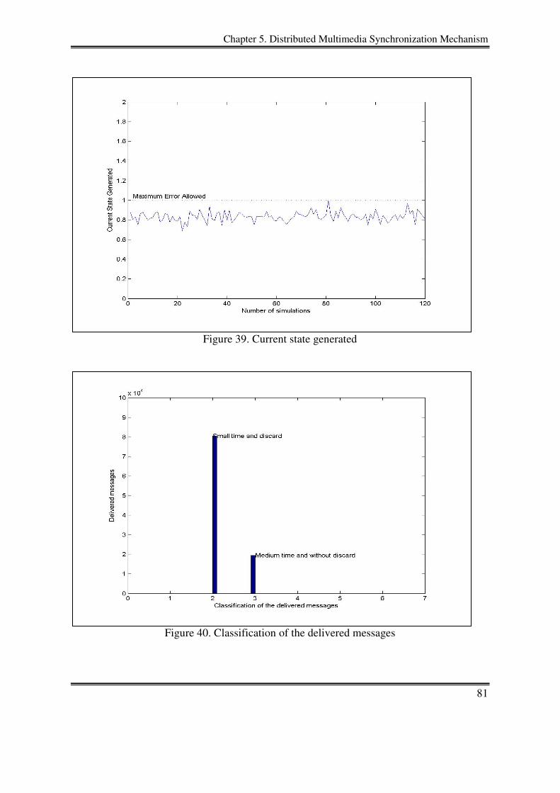
Chapter 5. Distributed Multimedia Synchronization Mechanism
81
Figure 39. Current state generated
Figure 40. Classification of the delivered messages
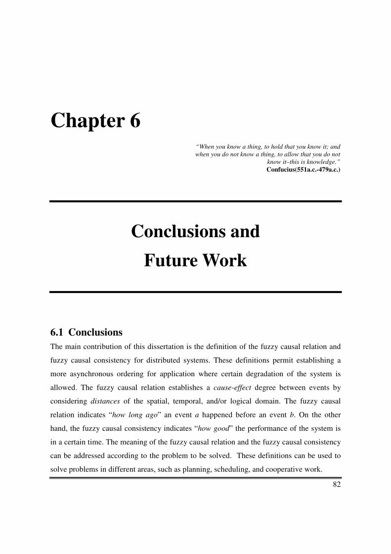
82
Chapter 6
“When you know a thing, to hold that you know it; and when you do not know a thing, to allow that you do not
know it–this is knowledge.” Confucius(551a.c.-479a.c.)
Conclusions and
Future Work
6.1 Conclusions
The main contribution of this dissertation is the definition of the fuzzy causal relation and
fuzzy causal consistency for distributed systems. These definitions permit establishing a
more asynchronous ordering for application where certain degradation of the system is
allowed. The fuzzy causal relation establishes a cause-effect degree between events by
considering distances of the spatial, temporal, and/or logical domain. The fuzzy causal
relation indicates “how long ago” an event a happened before an event b. On the other
hand, the fuzzy causal consistency indicates “how good” the performance of the system is
in a certain time. The meaning of the fuzzy causal relation and the fuzzy causal consistency
can be addressed according to the problem to be solved. These definitions can be used to
solve problems in different areas, such as planning, scheduling, and cooperative work.
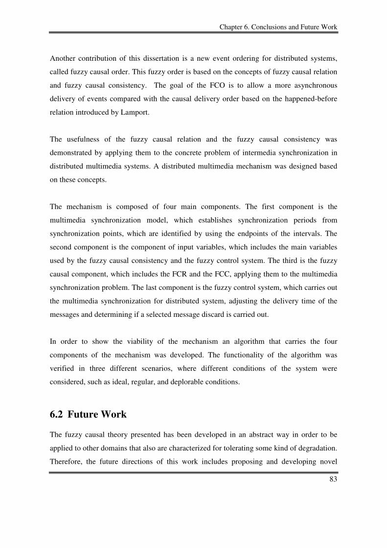
Chapter 6. Conclusions and Future Work
83
Another contribution of this dissertation is a new event ordering for distributed systems,
called fuzzy causal order. This fuzzy order is based on the concepts of fuzzy causal relation
and fuzzy causal consistency. The goal of the FCO is to allow a more asynchronous
delivery of events compared with the causal delivery order based on the happened-before
relation introduced by Lamport.
The usefulness of the fuzzy causal relation and the fuzzy causal consistency was
demonstrated by applying them to the concrete problem of intermedia synchronization in
distributed multimedia systems. A distributed multimedia mechanism was designed based
on these concepts.
The mechanism is composed of four main components. The first component is the
multimedia synchronization model, which establishes synchronization periods from
synchronization points, which are identified by using the endpoints of the intervals. The
second component is the component of input variables, which includes the main variables
used by the fuzzy causal consistency and the fuzzy control system. The third is the fuzzy
causal component, which includes the FCR and the FCC, applying them to the multimedia
synchronization problem. The last component is the fuzzy control system, which carries out
the multimedia synchronization for distributed system, adjusting the delivery time of the
messages and determining if a selected message discard is carried out.
In order to show the viability of the mechanism an algorithm that carries the four
components of the mechanism was developed. The functionality of the algorithm was
verified in three different scenarios, where different conditions of the system were
considered, such as ideal, regular, and deplorable conditions.
6.2 Future Work
The fuzzy causal theory presented has been developed in an abstract way in order to be
applied to other domains that also are characterized for tolerating some kind of degradation.
Therefore, the future directions of this work includes proposing and developing novel
Chapter 6. Conclusions and Future Work
84
solutions to classical problems in distributed systems, to problems in emerging areas, such
as ubiquitous computing and sensor networks, and proposing and developing novel
solutions for the emerging area of multimedia sensor networks. Next, a general description
of these problems is presented.
As immediate work, the fuzzy causal relation, the fuzzy causal consistency, and the fuzzy
causal order can be considered to resolve classical problems of distributed systems, such as
the followings:
• Detection of concurrent messages and establishing their delivery order. The research
could be focused on how the fuzzy precedence can be used to determine certain
order among the concurrent messages according to their temporal and logical
dependencies by using the FCR.
• Establishment of checkpoints by using the fuzzy causal consistency without
blocking the execution of parallel programs while checkpointing. If the checkpoints
are carried out in a loose manner, certain advantages in terms of low overhead in
failure-free execution, simplicity of recovery, and garbage collection, could be
obtained.
In a future stage, the fuzzy causal theory could be applied in the ubiquitous computing
environments and sensor networks.
• Ubiquitous computing environments are typically based upon ad hoc networks of
mobile computing devices. These devices may be equipped with sensor hardware to
sense the physical environment and may be attached to real world artifacts to form
so–called smart things. The data sensed by various smart things can then be
combined to derive knowledge about the environment, which in turn enables the
smart things to “react” intelligently to their environment. For this so–called sensor
fusion, temporal relationships (X happened before Y) and real–time issues (X and Y
happened within a certain time interval) play an important role. Thus physical time
and clock synchronization are crucial in such environments. However, due to the
characteristics of sparse ad hoc networks, classical clock synchronization algorithms
are not applicable in this setting. Hence, the synchronization of the temporal
Chapter 6. Conclusions and Future Work
85
dependencies could be carried out based on the fuzzy causal theory developed in
this dissertation.
A long term research focus is to apply the fuzzy theory to multimedia sensor networks.
• Multimedia sensor networks are a new and emerging type of sensor networks that
contain sensor nodes equipped with cameras, microphones, and other sensors,
producing multimedia content. These interconnected devices are able to
ubiquitously retrieve multimedia content, such as video and audio streams, still
images, and scalar sensor data from the environment. The multimedia sensor
networks have the potential to enable a large class of applications, ranging from
assisting the elderly in public spaces to border protection, which benefit from the
use of numerous sensor nodes that deliver multimedia content. Hence, in order to
determine relations between the data recollected from the sensors to reproduce and
monitor these scenarios, the fuzzy causal theory introduced in this dissertation could
be used.
86
References
[1]. A. Abouaissa, A. Benslimane. “A Multicast Synchronization Protocol for Real
Time Distributed Systems”. IEEE Proceedings of International Conference on
Networks, ICON '99, pp. 21- 28.
[2]. Aguilar José, 2004, “Dynamic Random Fuzzy Cognitive Maps”, Journal of
Computer Science and Systems, Volume 7, Number 004, Editorial Computing
Research Center of the IPN, Distrito Federal, México, ISSN 1405-5546, pp. 260-
271, Abril-Junio 2004.
[3]. André L. V. Coelho, Alberto B. Raposo, Ivan L. M. Ricarte. “Bringing Flexibility
to the Specification and Coordination of Temporal Dependencias among
Multimedia Components”. VII Simposio Brasileiro de Sistemas Multimídia e
Hipermídia, Florianópolis, Brazil, SBC. 2001, pp. 37-52.
[4]. Andrzej Duda, Chérif Keramane. “Structured temporal Composition of Multimedia
Data”. Proceedings of the International Workshop on Multi-Media Database
Management Systems (IW-MMDBMS), August 28-30, 1995, Blue Mountain Lake,
New York. IEEE-CS Press, 1995, ISBN 0-8186-7168-8, pp.136-142.
[5]. Birman K., Schiper A., and Stephenson P., 1991, Lightweight Causal and Atomic
Group Multicast, ACM Trans. Compt. Syst. Vol. 9, No. 3, ISSN:0734-2071, pp.
272-314, Aug. 1991.
[6]. Colin Perkins, RTP - Audio and Video for the Internet, Addison-Wesley, 2003.
ISBN 0-672-32249-8.
[7]. Ernst Biersack, Christoph Bernhardt, Werner Geyer. “Intra- and Inter-Stream
Synchronization of Stored Multimedia Streams”. Proceedings of the IEEE
International Conference on Multimedia Computing and Systems, ICMCS 1996, pp.
372-381.
[8]. Fidge C. J. “Partial Orders for Parallel Debugging”. Proceedings of the 1988 ACM
SIGPLAN and SIGOPS Workshop on Parallel and Distributed Debugging, May
1988, pp.183-194.
87
[9]. H.P. Dommel and S. Verma. “Multipoint Synchronization Protocol”. Proceedings
of the IEEE International Conference on Systems, Man and Cybernetics (SMC'04),
The Hague, The Netherlands, Oct. 10-13, 2004.
[10]. Haining Liu and Magda El Zarki. “A synchronization control scheme for real-time
streaming multimedia applications”. Proceedings of Packet Video, 2003, France.
[11]. Haj A. and . Xue C-, 1997, Synchronization in Multimedia Data Retrieval,
International Journal of Network Management, John Wiley & Sons, Inc. New York,
NY, USA Volume 7, Issue 1, ISSN:1099-1190, pp. 33–62, January–February 1997.
[12]. Helen Cameron, Peter King, Howard Bowman, and Simon Thompson.
“Synchronization in Multimedia Documents”. Proceedings of the 7th International
Conference on Electronic Publishing, Held Jointly with the 4th International
Conference on Raster Imaging and Digital Typography: Electronic Publishing,
Artistic Imaging, and Digital Typography”, Lecture Notes In Computer Science;
Volume 1375, 1998, ISBN:3-540-64298-6, pp. 355–369.
[13]. Hua Zhu Guoping Zeng Chlamtac , I. “Control scheme analysis for multimedia
inter- and intra-stream synchronization”. Proceedings of the IEEE International
Conference on Communications, 11-15 May, 2003, Volume: 1, ISBN: 0-7803-
7802-4, pp. 7- 11.
[14]. Hung T. Nguyen A First Course in Fuzzy Logic, CRC; 2 edition (July 21, 1999),
ISBN-10: 0849316596.
[15]. ISO. “Information processing - Text and Office Systems - Standard Generalized
Markup Language (SGML)”. 1986. ISO-IS 8879.
[16]. J.P. Courtiat, L.F.R.C. Carmo, and R.C. de Oliveira. “A General-Purpose
Multimedia Synchronization Mechanism Based on Causal Relations”. IEEE Journal
on Selected Areas in Communications, Volume 14, Number 1, January 1996, pp.
185-195.
[17]. Kaladji, F. Ishibashi, Y. and Tasaka, S. “Subjective Assessment of Stored Media
Synchronization Quality in the VTR Algorithm”. IEICE Transactions On
Communications E Series B, 1999, Volume 82, Number 1. pp. 24-33.
88
[18]. Kien A. Hua and Duc A. Tran. “Range Multicast for Video on Demand”. To
appear in Journal of Multimedia Tools and Applications, Volume 27, Issue 3,
ISSN:1380-7501, December 2005, pp. 367 - 391 .
[19]. Kshemkalyani Ajay D. “Temporal Interactions of Intervals in Distributed
Systems”. Journal of Computer and System Science, Volume 52, Number 3, June
1996 pp. 287-298.
[20]. Lars C. Wolf and Carsten Griwodz and Ralf Steinmetz. “Multimedia
Communication”. Proceedings of the IEEE, Volume 85, Number 12, December
1997, pp. 1915-1933.
[21]. Leslie Lamport, 1978, “Time, Clocks, and the Ordering of Events in a Distributed
System”, Communications ACM, Volume 21, Number 7, ISSN:0001-0782, pp. 558-
565, July 1978.
[22]. Lopez, E., J. Estudillo, J. Fanchon, S. Pomares, 2005, “A Fault-tolerant Causal
Broadcast Algorithm to be Applied to Unreliable Networks”, Proc. 17th
International Conference on Parallel and Distributed Computing and Systems, pp.
465-470, 2005.
[23]. Louise Lamont, Lian Li, Renaud Brimont, Nicolas D. Georganas.
“Synchronization of Multimedia Data for a Multimedia News-on-Demand
Application”. IEEE Journal on Selected Areas in Communications, Volume 14,
Number 1, January 1996, pp. 264-278 .
[24]. M. da G. Pimentel, L. Baldochi, jr., F. Fagundes, C. Teixera, “Temporal Relations
in Multimedia Objects: WWW Presentation from HyTime Specification”.
Proceeding of IEEE PROMS-MmNet'97, November 24-27, 1997, Santiago, Chile.
[25]. Michal Haindl: “A New Multimedia Synchronization Model”. IEEE Journal on
Selected Areas in Communications, Volume 14, Number 1, January 1996, pp. 73-
83.
[26]. Morales Rosales Luis A. Algoritmo de Sincronización de flujos continuos en
tiempo real. Tesis de Maestría en Ciencias Computacionales, INAOE. Num.
XM1086. Clasificación: XMM-M67-2005-XM1086, Tonantzintla Puebla, México.
Año 2005, pp. 83.
89
[27]. Morales Rosales Luis, Pomares Hernandez Saul, “A Temporal Synchronization
Mechanism for Real-Time Distributed Continuous Media,” International
Conference on Signal Processing and Multimedia Applications (SIGMAP’06),
Setubal, Portugal, Aug. 2006, INSTICC Press, ISBN 972-8865-64-3, pp. 302-309.
[28]. Nipun Agarwal, Sang Hyuk Son. “A Model for Specification and Synchronization
of Data for Distributed Multimedia Applications”. Multimedia Tools and
Applications, Volume 3, Number 2, September 1996, pp. 79-104.
[29]. Pantelis Balaouras, Ioannis Stavrakakis, Lazaros F. Merakos. “Potential and
limitations of a teleteaching environment based on H.323 audio-visual
communication systems”. Computer Networks, volume 34, number 6, December
2000, pp. 945-958.
[30]. Patrick Schmitz, “The SMIL 2.0 Timing and Synchronization Model: Using Time
in Documents”. Technical report, MSR-TR-2001-01, Microsoft research. January 2,
2001.
[31]. Pomares Hernandez Saul E., Morales Rosales Luis A., Estudillo Ramirez Jorge,
and Rodriguez Gomez Gustavo, “Logical Mapping: An Intermedia Synchronization
Model for Multimedia Distributed Systems,” Journal of Multimedia, Eds. Academy
Publisher, Vol. 3 No.5, 2008, ISSN: 1796-2048, pp. 33-41.
[32]. Ramaprabhu Janakiraman, B.E. Thesis of master science. Server Institute of
Washington University. Saint Louis Missouri, USA. December 2002. pp. 30
[33]. Ramaprabhu Janakiraman, Marcel Waldvogel and Lihao Xu. “Fuzzycast: Efficient
Video-on-demand over Multicast”. Proceedings INFOCOM 2002, New York, NY,
USA, June 2002.
[34]. Roberto Baldoni and Ravi Prakash and Michel Raynal and Mukesh Singhal.
“Efficient ∆-causal broadcasting”. International Journal of Computer Systems
Science and Engineering, Volume 13, Number 5, 1998, pp. 263-269.
[35]. Roberto Baldoni, Achour Mostéfaoui, Michel Raynal. “Causal Delivery of
Messages with Real-Time Data in Unreliable Networks”. Real-Time Systems,
Volume 10, Number 3, May 1996 pp. 245-262.
[36]. Roberto Baldoni, Achour Mostéfaoui, Michel Raynal. “Efficient Causally Ordered
Communications for Multimedia Real-Time Applications”. The 4th International
90
Symposium on High Performance Distributed Computing (HPDC '95), Washington,
DC, USA, August 2-4, 1995, pp. 140-147
[37]. Roberto Baldoni, Michel Raynal, Ravi Prakash, Mukesh Singhal. “Broadcast with
Time and Causality Constraints for Multimedia Applications”. 22rd EUROMICRO
Conference '96, Beyond 2000: Hardware and Software Design Strategies, 1996, pp.
617-624.
[38]. Shimamura K., Tanaka K., andTakizawa M. “Object-Causally Ordered Group
Protocol for Distributed Multimedia Systems”. Proceedings of the 15th
International Conference on Information Networking, ICOIN'01, 31 January-2
February 2001, Beppu City, Oita, Japan. IEEE Computer Society, pp. 921-926.
[39]. Shimamura, K.; Tanaka, K.; Takizawa, M. “Group communication protocol for
multimedia applications”. Proceedings. 2001 International Conference on
Computer Networks and Mobile Computing, 16-19 October, 2001, pp. 303–308.
[40]. Silvana. Badaloni, Massimiliano Giacomin, 2006, The algebra IAfuz: a
Framework for Qualitative Fuzzy Temporal Reasoning, Artificial
Intelligence, Volume 170, Number 10, Elsevier, pp. 872-908, July 2006.
[41]. Susanne Boll, Wolfgang Klas, Utz Westermann, “A Comparison of Multimedia
Document Models Concerning Advanced Requirements”. Technical Report - Ulmer
Informatik-Berichte Nr 99-01, February 1999, Computer Science Department,
University of Ulm, Germany.
[42]. T. Bray, J. Paoli and C. M. Sperberg-McQueen. “Extensible Markup Language
(XML) 1.0 W3C-Recommendation 10-February-1998”. W3C,
URL:http://www.w3.org/TR/1998/REC-xml-19980210, February 1998.
[43]. Tachikawa T., and Takizawa, M., "Multimedia Intra-Group Communication
Protocol". The 4th International Symposium on High Performance Distributed
Computing (HPDC '95), IEEE Conputer Society, Washington, DC, USA, August 2-
4, 1995, pp.180-187.
[44]. Tachikawa T., Makoto Takizawa. “∆-Causality in Wide-Area Group
Communications”. Proceedings of the International Conference on Parallel and
Distributed Systems (ICPADS '97), 11-13 December 1997, Seoul, Korea, IEEE
Computer Society 1997, ISBN 0-8186-8227-2, pp. 260-267.
91
[45]. Tachikawa, T. and Takizawa, M. “Group Communication for Real-time
Continuous Media”. Proceeding of International Symposium on .Multimedia
Systems, Japan, 1996, pp. 118-125.
[46]. Thomas D. C. Little, Arif Ghafoor. “Synchronization and Storage Models for
Multimedia Objects”. IEEE Journal on Selected Areas in Communications”,
Volume 8, Number 3, April 1990, pp. 413-427.
[47]. Thomas Meyer-Boudnik, Wolfgang Effelsberg. “MHEG Explained”. IEEE
MultiMedia, Volume 2, Number 1, Spring 1995, pp. 26-38.
[48]. Thomas Wahl, Kurt Rothermel. “Representing Time in Multimedia Systems”.
Proceedings of the International Conference on Multimedia Computing and
Systems, May 14-19, 1994, Boston, Massachusetts. ISBN 0-8186-5530-5, pp. 538-
543.
[49]. Tomoya Enokido, Sei-ichi Hatori, Takuya Tojo Makoto Takizawa. “Group
Communication in Distributed Multimedia Objects”. Proceeding of The Eighth
IEEE International Workshop on Object-Oriented Real-Time Dependable Systems
(WORDS 2003), 2003, pp. 258.
[50]. Venkat Rangan, Shrihari Sampath Kumar, Sreerang Rajan. “Continuity and
Synchronization in MPEG”. IEEE Journal on Selected Areas in Communications,
Volume 14, Number 1, January 1996, pp. 52-60.
[51]. Xingye Yu, Yang Yang, Zhiguang Shan, “Synchronization Technology for
Multimedia Communication in Digital Earth”. Towards Digital Earth-Proceedings
of the International Symposium On Digital Earth, Science Press, Editada por
Guanhua Xu and Yuntai Chen, Nov. 29-Dec. 2, Beijing, China, 1999, ISBN: 7-03-
005600-0.
[52]. Youhei Timura, Katsuya Tanaka, Makoto Takizawa. “Causal Precedent Relations
among Messages in Object-Based Systems”. Eigth International Conference on
Parallel and Distributed Systems (ICPADS 2001), 26-29 June 2001, KyongJu City,
Korea, ISBN 0-7695-1153-8, pp. 355-362.
[53]. Yutaka Ishibashi, Shuji Tasaka, Yoshiro Tachibana. “A Media Synchronization
Scheme with Causality Control in Network Environments”. Proceedings 26th
Conference on Local Computer Networks, Lowell, Massachusetts, USA, 17-20
92
October 1999, IEEE Computer Society, pp. 232-241.
[54]. Zhou Y., Murata T., 2001, Modeling and Analysis of Distributed Multimedia
Synchronization by Extended Fuzzy-Timing Petri Nets, Transactions of the Society
for Design and Process Science, Volume 5, Number 4, ISSN:1092-0617, pp. 23-37,
December 2001.

93
Appendixes
Appendix A. Happened-before relation for Intervals
The happened-before relation proposed by Morales and Pomares in [26, 27] establish that:
if the elements of an interval are sequentially ordered, then ensuring partial causal order on
the interval endpoints is sufficient to ensure causal ordering at an interval level. This
relation was formally defined as follows:
Definition 9. The relation “→I ” is accomplished if it satisfies the following two conditions:
1) A →I B if a+→M’ b-
2) A →I B if ∃C | (a+ →M’ c- ∧ c+→M’ b
-)
Where a+ and b- are the final and initial send events (or messages) of A and B respectively,
c- and c+ are the endpoints of C, and →M’ is the partial causal order (Definition 2) induced
on M’ ⊆ M, where M’, in this case, is the subset composed by the endpoint messages of the
intervals in I.
The simultaneous relation to be applied to intervals is defined as follows:
Definition 10. Two intervals A, B are said to be simultaneous “ ||| ” if the following
condition is satisfied:
A ||| B ⇒ a- || b- ∧ a+ || b
+
The definition above means that one interval A can take place at the “same time” as another
interval B.
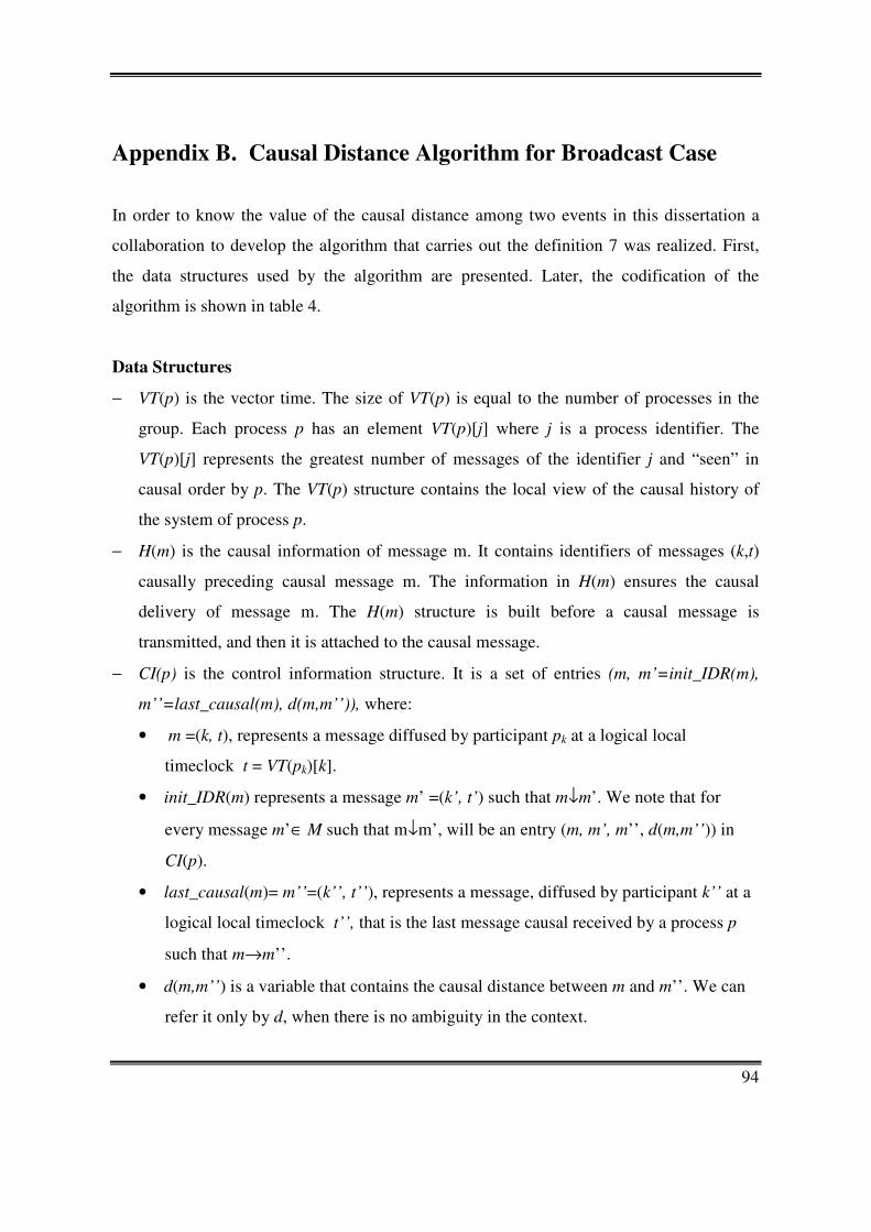
94
Appendix B. Causal Distance Algorithm for Broadcast Case
In order to know the value of the causal distance among two events in this dissertation a
collaboration to develop the algorithm that carries out the definition 7 was realized. First,
the data structures used by the algorithm are presented. Later, the codification of the
algorithm is shown in table 4.
Data Structures
− VT(p) is the vector time. The size of VT(p) is equal to the number of processes in the
group. Each process p has an element VT(p)[j] where j is a process identifier. The
VT(p)[j] represents the greatest number of messages of the identifier j and “seen” in
causal order by p. The VT(p) structure contains the local view of the causal history of
the system of process p.
− H(m) is the causal information of message m. It contains identifiers of messages (k,t)
causally preceding causal message m. The information in H(m) ensures the causal
delivery of message m. The H(m) structure is built before a causal message is
transmitted, and then it is attached to the causal message.
− CI(p) is the control information structure. It is a set of entries (m, m’=init_IDR(m),
m’’=last_causal(m), d(m,m’’)), where:
• m =(k, t), represents a message diffused by participant pk at a logical local
timeclock t = VT(pk)[k].
• init_IDR(m) represents a message m’ =(k’, t’) such that m↓m’. We note that for
every message m’∈ M such that m↓m’, will be an entry (m, m’, m’’, d(m,m’’)) in
CI(p).
• last_causal(m)= m’’=(k’’, t’’), represents a message, diffused by participant k’’ at a
logical local timeclock t’’, that is the last message causal received by a process p
such that m→m’’.
• d(m,m’’) is a variable that contains the causal distance between m and m’’. We can
refer it only by d, when there is no ambiguity in the context.
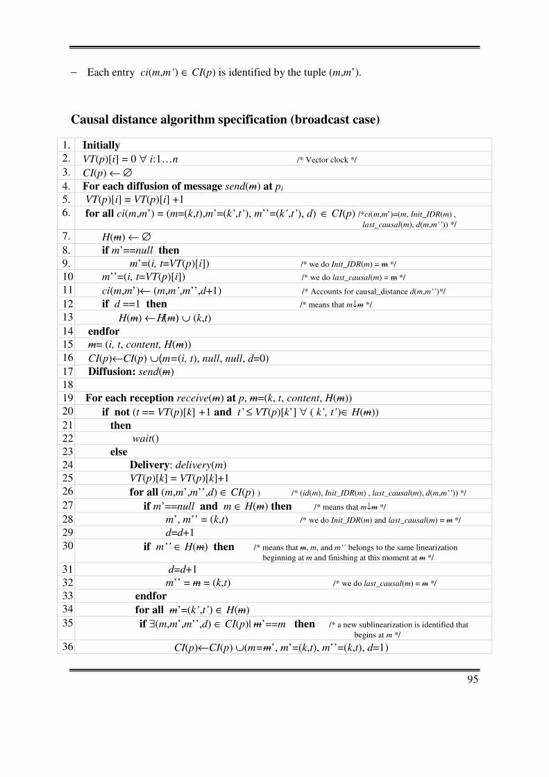
95
− Each entry ci(m,m’) ∈ CI(p) is identified by the tuple (m,m’).
Causal distance algorithm specification (broadcast case)
1. Initially
2. VT(p)[i] = 0 ∀ i:1…n /* Vector clock */ 3. CI(p) ← ∅ 4. For each diffusion of message send(m) at pi 5. VT(p)[i] = VT(p)[i] +1 6. for all ci(m,m’) = (m=(k,t),m’=(k’,t’), m’’=(k’,t’), d) ∈ CI(p) /*ci(m,m’)=(m, Init_IDR(m) ,
last_causal(m), d(m,m’’)) */ 7. H(m) ← ∅ 8. if m’==null then 9. m’=(i, t=VT(p)[i]) /* we do Init_IDR(m) = m */ 10. m’’=(i, t=VT(p)[i]) /* we do last_causal(m) = m */ 11. ci(m,m’)← (m,m’,m’’,d+1) /* Accounts for causal_distance d(m,m’’)*/ 12. if d ==1 then /* means that m↓m */ 13. H(m) ←Η(m) ∪ (k,t) 14. endfor
15. m= (i, t, content, H(m)) 16. CI(p)←CI(p) ∪(m=(i, t), null, null, d=0) 17. Diffusion: send(m) 18. 19. For each reception receive(m) at p, m=(k, t, content, H(m)) 20. if not (t == VT(p)[k] +1 and t’ ≤ VT(p)[k’] ∀ ( k’, t’)∈ H(m)) 21. then
22. wait() 23. else
24. Delivery: delivery(m) 25. VT(p)[k] = VT(p)[k]+1 26. for all (m,m’,m’’,d) ∈ CI(p) ) /* (id(m), Init_IDR(m) , last_causal(m), d(m,m’’)) */ 27. if m’==null and m ∈ H(m) then /* means that m↓m */
28. m’, m’’ = (k,t) /* we do Init_IDR(m) and last_causal(m) = m */ 29. d=d+1 30. if m’’ ∈ H(m) then /* means that m, m, and m’’ belongs to the same linearization
beginning at m and finishing at this moment at m */ 31. d=d+1 32. m’’ = m = (k,t) /* we do last_causal(m) = m */ 33. endfor
34. for all m’=(k’,t’) ∈ H(m) 35. if ∃(m,m’,m’’,d) ∈ CI(p)| m’==m then /* a new sublinearization is identified that
begins at m */ 36. CI(p)←CI(p) ∪(m=m’, m’=(k,t), m’’=(k,t), d=1)
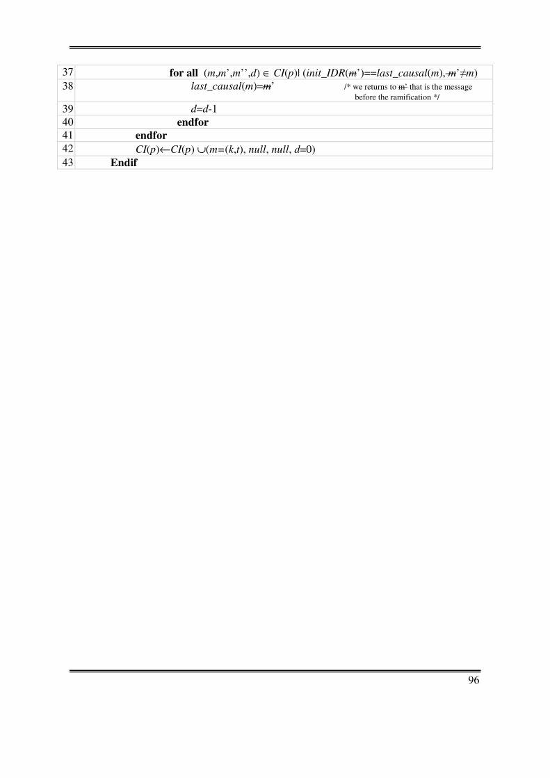
96
37. for all (m,m’,m’’,d) ∈ CI(p)| (init_IDR(m’)==last_causal(m), m’≠m) 38. last_causal(m)=m’ /* we returns to m’ that is the message
before the ramification */ 39. d=d-1 40. endfor
41. endfor
42. CI(p)←CI(p) ∪(m=(k,t), null, null, d=0) 43. Endif
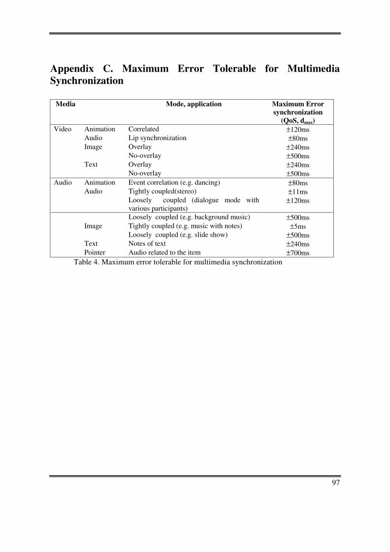
97
Appendix C. Maximum Error Tolerable for Multimedia
Synchronization
Media Mode, application Maximum Error
synchronization
(QoS, dmax)
Video Animation Correlated ±120ms Audio Lip synchronization ±80ms Image Overlay ±240ms No-overlay ±500ms Text Overlay ±240ms No-overlay ±500ms Audio Animation Event correlation (e.g. dancing) ±80ms Audio Tightly coupled(stereo) ±11ms Loosely coupled (dialogue mode with
various participants) ±120ms
Loosely coupled (e.g. background music) ±500ms Image Tightly coupled (e.g. music with notes) ±5ms Loosely coupled (e.g. slide show) ±500ms Text Notes of text ±240ms Pointer Audio related to the item ±700ms
Table 4. Maximum error tolerable for multimedia synchronization