Embed Size (px)
Citation preview
Distributed Localization Algorithms
Koen Langendoen and Niels ReijersDelft University of Technology
Faculty of Electrical Engineering, Mathematics and Computer ScienceMekelweg 4, 2628CD Delft, The [email protected]@ewi.tudelft.nl
1 Introduction
New technology offers new opportunities, but it also introduces new problems. This is particularlytrue for sensor networks where the capabilities of individual nodes are very limited. Hence,collaboration between nodes is required, but energy conservation is a major concern, which impliesthat communication should be minimized. These conflicting objectives require unorthodox solutionsfor many situations.
A recent survey by Akyildiz et al. discusses a long list of open research issues that must beaddressed before sensor networks can become widely deployed [1]. The problems range from thephysical layer (low-power sensing, processing, and communication hardware) all the way up to theapplication layer (query and data dissemination protocols). In this chapter we address the issue oflocalization in ad-hoc sensor networks. That is, we want to determine the location of individualsensor nodes without relying on external infrastructure (base stations, satellites, etc.).
The localization problem has received considerable attention in the past, as many applicationsneed to know where objects or persons are, and hence various location services have been created.Undoubtedly, the Global Positioning System (GPS) is the most well-known location service in usetoday. The approach taken by GPS, however, is unsuitable for low-cost, ad-hoc sensor networkssince GPS is based on extensive infrastructure (i.e. satellites). Likewise solutions developed in thearea of robotics [2, 13, 20] and ubiquitous computing [10] are generally not applicable for sensornetworks as they require too much processing power and energy.
Recently a number of localization systems have been proposed specifically for sensor net-works [4, 5, 6, 7, 9, 14, 16, 17, 19]. We are interested in truly distributed algorithms that can beemployed on large-scale ad-hoc sensor networks (100+ nodes). Such algorithms should be:
1. self-organizing (i.e. do not depend on global infrastructure),
2. robust (i.e. be tolerant to node failures and range errors), and
3. energy efficient (i.e. require little computation and, especially, communication).
1
2
These requirements immediately rule out some of the proposed localization algorithms for sensornetworks. In this chapter, we carry out a thorough sensitivity analysis on three algorithms thatdo meet the above requirements to determine how well they perform under various conditions. Inparticular, we study the impact of the following parameters: range errors, connectivity (density),and anchor fraction. These algorithms differ in their position accuracy, network coverage, inducednetwork traffic, and processor load. Given the (slightly) different design objectives for the threealgorithms, it is no surprise that each algorithm outperforms the others under a specific set ofconditions. Under each condition, however, even the best algorithm leaves much room for improvingaccuracy and/or increasing coverage.
In this chapter we will
1. identify a common, 3-phase, structure in the selected distributed localization algorithms.
2. identify a generic optimization applicable to all algorithms.
3. provide a detailed comparison on a single (simulation) platform.
4. show that there is no algorithm that performs best, and that there exists room for improvementin most cases.
Section 2 discusses the selection, generic structure, and operation of three distributed localizationalgorithms for large-scale ad-hoc sensor networks. These algorithms are compared on a simulationplatform, which is described in Section 3. Section 4 presents intermediate results for the individualphases, while Section 5 provides a detailed overall comparison and an in-depth sensitivity analysis.Finally, we give conclusions in Section 6.
2 Localization algorithms
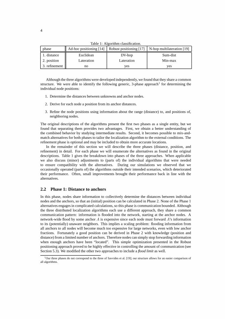
Before discussing distributed localization in detail, we first outline the context in which thesealgorithms have to operate. A first consideration is that the requirement for sensor networks tobe self-organizing implies that there is no fine control over the placement of the sensor nodeswhen the network is installed (e.g., when nodes are dropped from an airplane). Consequently, weassume that nodes are randomly distributed across the environment. For simplicity and ease ofpresentation we limit the environment to 2 dimensions, but all algorithms are capable of operating in3D. Figure 1 shows an example network with 25 nodes; pairs of nodes that can communicate directlyare connected by an edge. The connectivity of the nodes in the network (i.e. the average number ofneighbors) is an important parameter that has a strong impact on the accuracy of most localizationalgorithms (see Sections 4 and 5). It is initially determined by the node density and radio range, andin some cases it can be adjusted dynamically by changing the transmit power of the RF radio.
In some application scenarios, nodes may be mobile. In this paper, however, we focus on staticnetworks, where nodes do not move, since this is already a challenging condition for distributedlocalization. We assume that some anchor nodes have a priori knowledge of their own positionwith respect to some global coordinate system. Note that anchor nodes have the same capabilities(processing, communication, energy consumption, etc.) as all other sensor nodes with unknownpositions; we do not consider approaches based on an external infrastructure with specialized beaconnodes (access points) as used in, for example, the GPS-less [4], Cricket [15], and RADAR [3]location systems. Ideally the fraction of anchor nodes should be as low as possible to minimize theinstallation costs. Our simulation results show that, fortunately, most algorithms are rather insensitiveto the number of anchors in the network.
The final element that defines the context of distributed localization is the capability to measurethe distance between directly connected nodes in the network. From a cost perspective it is attractive
3
AnchorUnknown
Figure 1: Example network topology.
to use the RF radio for measuring the range between nodes, for example, by observing the signalstrength. Experience has shown, however, that this approach yields poor distance estimates [11, 24,18]. Much better results are obtained by time-of-flight measurements, particularly when acousticand RF signals are combined [8, 18, 19]; accuracies of a few percent of the transmission range arereported. However, this requires extra hardware on the sensor boards.
Several different ways of dealing with the problem of inaccurate distance information have beenproposed. The APIT [9] algorithm by He et al. only needs distance information accurate enoughfor two nodes determine which of them is closest to an anchor. GPS-less [4] by Bulusu et al. andDV-hop [14] by Niculescu and Nath. do not use distance information at all, and are based on topologyinformation only. Ramadurai and Sichitiu [16] propose a probabilistic approach to the localizationproblem. Not only the measured distance, but also the confidence in the measurement is used.
It is important to realize that the main three context parameters (connectivity, anchor fraction,and range errors) are dependent. Poor range measurements can be compensated for by using manyanchors and/or a high connectivity. This chapter provides insight in the complex relation betweenconnectivity, anchor fraction, and range errors for a number of distributed localization algorithms.
2.1 Generic approach
From the known localization algorithms specifically proposed for sensor networks, we selected thethree approaches that meet the basic requirements for self-organization, robustness, and energy-efficiency:
1. Ad-hoc positioning by Niculescu and Nath [14],
2. N-hop multilateration by Savvides et al. [19], and
3. Robust positioning by Savarese et al. [17].
The other approaches often include a central processing element (e.g., ‘convex optimization’ byDoherty et al. [7]), rely on an external infrastructure (e.g., ‘GPS-less’ by Bulusu et al. [4]), or inducetoo much communication (e.g., ‘GPS-free’ by Capkun et al. [5]). The three selected algorithms arefully distributed and use local broadcast for communication with immediate neighbors. This lastfeature allows them to be executed before any multi-hop routing is in place, hence, they can supportefficient location-based routing schemes like GAF [23].
4
Table 1: Algorithm classification.phase Ad-hoc positioning [14] Robust positioning [17] N-hop multilateration [19]
1. distance Euclidean DV-hop Sum-dist
2. position Lateration Lateration Min-max
3. refinement no yes yes
Although the three algorithms were developed independently, we found that they share a commonstructure. We were able to identify the following generic, 3-phase approach1 for determining theindividual node positions:
1. Determine the distances between unknowns and anchor nodes.
2. Derive for each node a position from its anchor distances.
3. Refine the node positions using information about the range (distance) to, and positions of,neighboring nodes.
The original descriptions of the algorithms present the first two phases as a single entity, but wefound that separating them provides two advantages. First, we obtain a better understanding ofthe combined behavior by studying intermediate results. Second, it becomes possible to mix-and-match alternatives for both phases to tailor the localization algorithm to the external conditions. Therefinement phase is optional and may be included to obtain more accurate locations.
In the remainder of this section we will describe the three phases (distance, position, andrefinement) in detail. For each phase we will enumerate the alternatives as found in the originaldescriptions. Table 1 gives the breakdown into phases of the three approaches. When applicablewe also discuss (minor) adjustments to (parts of) the individual algorithms that were neededto ensure compatibility with the alternatives. During our simulations we observed that weoccasionally operated (parts of) the algorithms outside their intended scenarios, which deterioratedtheir performance. Often, small improvements brought their performance back in line with thealternatives.
2.2 Phase 1: Distance to anchors
In this phase, nodes share information to collectively determine the distances between individualnodes and the anchors, so that an (initial) position can be calculated in Phase 2. None of the Phase 1alternatives engages in complicated calculations, so this phase is communication bounded. Althoughthe three distributed localization algorithms each use a different approach, they share a commoncommunication pattern: information is flooded into the network, starting at the anchor nodes. Anetwork-wide flood by some anchor A is expensive since each node must forward A’s informationto its (potentially) unaware neighbors. This implies a scaling problem: flooding information fromall anchors to all nodes will become much too expensive for large networks, even with low anchorfractions. Fortunately a good position can be derived in Phase 2 with knowledge (position anddistance) from a limited number of anchors. Therefore nodes can simply stop forwarding informationwhen enough anchors have been “located”. This simple optimization presented in the Robustpositioning approach proved to be highly effective in controlling the amount of communication (seeSection 5.3). We modified the other two approaches to include a flood limit as well.
1Our three phases do not correspond to the three of Savvides et al. [19]; our structure allows for an easier comparison ofall algorithms.
5
Sum-dist
The most simple solution for determining the distance to the anchors is simply adding the rangesencountered at each hop during the network flood. This is the approach taken by the N-hopmultilateration approach, but it remained nameless in the original description [19]; we name itSum-dist in this paper. Sum-dist starts at the anchors, who send a message including their identity,position, and a path length set to 0. Each receiving node adds the measured range to the path lengthand forwards (broadcasts) the message if the flood limit allows it to do so. Another constraint isthat when the node has received information about the particular anchor before, it is only allowed toforward the message if the current path length is less than the previous one. The end result is thateach node will have stored the position and minimum path length to at least flood limit anchors.
DV-hop
A drawback of Sum-dist is that range errors accumulate when distance information is propagatedover multiple hops. This cumulative error becomes significant for large networks with few anchors(long paths) and/or poor ranging hardware. A robust alternative is to use topological information bycounting the number of hops instead of summing the (erroneous) ranges. This approach was namedDV-hop by Niculescu and Nath [14], and Hop-TERRAIN by Savarese et al. [17]. Since the results ofDV-hop were published first we will use this name.
DV-hop essentially consists of two flood waves. After the first wave, which is similar to Sum-dist,nodes have obtained the position and minimum hop count to at least flood limit anchors. The secondcalibration wave is needed to convert hop counts into distances such that Phase 2 can computea position. This conversion consists of multiplying the hop count with an average hop distance.Whenever an anchor a1 infers the position of another anchor a2 during the first wave, it computesthe distance between them, and divides that by the number of hops to derive the average hop distancebetween a1 and a2. When calibrating, an anchor takes all remote anchors into account that it isaware of. When later, information on extra anchors is received, the calibration procedure is repeated.Nodes forward (broadcast) calibration messages only from the first anchor that calibrates them, whichreduces the total number of messages in the network.
Euclidean
A drawback of DV-hop is that it fails for highly irregular network topologies, where the variancein actual hop distances is very large. Niculescu and Nath have proposed another method, namedEuclidean, which is based on the local geometry of the nodes around an anchor. Again anchorsinitiate a flood, but forwarding the distance is more complicated than in the previous cases. When anode has received messages from two neighbors that know their distance to the anchor, and to eachother, it can calculate the distance to the anchor.
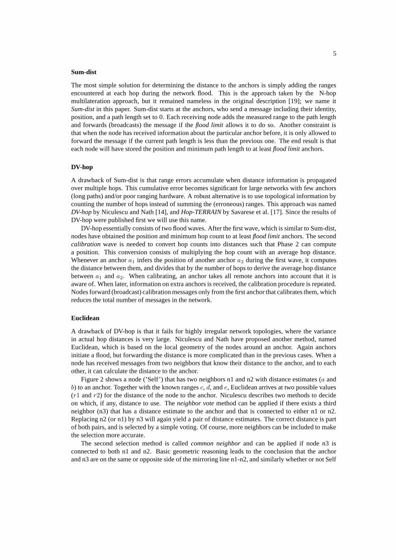
Figure 2 shows a node (’Self’) that has two neighbors n1 and n2 with distance estimates (a andb) to an anchor. Together with the known ranges c, d, and e, Euclidean arrives at two possible values(r1 and r2) for the distance of the node to the anchor. Niculescu describes two methods to decideon which, if any, distance to use. The neighbor vote method can be applied if there exists a thirdneighbor (n3) that has a distance estimate to the anchor and that is connected to either n1 or n2.Replacing n2 (or n1) by n3 will again yield a pair of distance estimates. The correct distance is partof both pairs, and is selected by a simple voting. Of course, more neighbors can be included to makethe selection more accurate.
The second selection method is called common neighbor and can be applied if node n3 isconnected to both n1 and n2. Basic geometric reasoning leads to the conclusion that the anchorand n3 are on the same or opposite side of the mirroring line n1-n2, and similarly whether or not Self
6
n2
n1
AnchorSelf’Self
bee
r1r2
ad
c
d
Figure 2: Determining distance using Euclidean.
and n3 are on the same side. From this it follows whether or not self and the anchor lay on the sameside.
To handle the uncertainty introduced by range errors Niculescu implements a safety mechanismthat rejects ill-formed (flat) triangles, which can easily derail the selection process by ‘neighbor vote’and ‘common neighbor’. This check verifies that the sum of the two smallest sides exceeds the largestside multiplied by a threshold, which is set to two times the range variance. For example, the triangleSelf-n1-n2 in Figure 2 is accepted when c + d > (1 + 2RangeV ar) × e. Note that the safety checkbecomes more strict as the range variance increases. This leads to a lower coverage, defined as thepercentage of non-anchor nodes for which a position was determined.
We now describe some modifications to Niculescu’s ‘neighbor vote’ method that remedy the poorselection of the location for Self in important corner cases. The first problem occurs when the twovotes are identical because, for instance, the three neighbors (n1, n2, and n3) are collinear. In thesecases it is hard to select the right alternative. Our solution is to leave equal vote cases unsolved,instead of picking an alternative and propagating an error with 50% chance. We filter all indecisivecases by adding the requirement that the standard deviation of the votes for the selected distance mustbe at most 1/3rd of the standard deviation of the other distance. The second problem that we addressis that of a bad neighbor with inaccurate information spoiling the selection process by voting fortwo wrong distances. This case is filtered out by requiring that the standard deviation of the selecteddistance is at most 5% of that distance.
To achieve good coverage, we use both the neighbor vote and common neighbor methods. Ifboth produce a result, we use the result from the modified ‘neighbor vote’ because we found it to bethe most accurate of the two. If both fail, the flooding process stops, leading to the situation wherecertain nodes are not able to establish the distance to enough anchor nodes. Sum-dist and DV-hop,on the other hand, never fail to propagate the distance and hop count, respectively.
2.3 Phase 2: Node position
In the second phase nodes determine their position based on the distance estimates to a numberof anchors provided by one of the three Phase 1 alternatives (Sum-dist, DV-hop, or Euclidean).The Ad-hoc positioning and Robust positioning approaches use lateration for this purpose. N-hopmultilateration, on the other hand, uses a much simpler method, which we named Min-max. In bothcases the determination of the node positions does not involve additional communication.
Lateration
The most common method for deriving a position is lateration, which is a form of triangulation.From the estimated distances (di) and known positions (xi, yi) of the anchors we derive the following
7
system of equations:
(x1 − x)2 + (y1 − y)2 = d1
2
...
(xn − x)2 + (yn − y)2 = dn
2
where the unknown position is denoted by (x, y). The system can be linearized by subtracting thelast equation from the first n − 1 equations.
x1
2− xn
2− 2(x1 − xn)x +
y1
2− yn
2− 2(y1 − yn)y = d1
2− dn
2
...
xn−1
2− xn
2− 2(xn−1 − xn)x +
yn−1
2− yn
2− 2(yn−1 − yn)y = dn−1
2− dn
2
Reordering the terms gives a proper system of linear equations in the form Ax=b, where
A =
2(x1 − xn) 2(y1 − yn)...
...
2(xn−1 − xn) 2(yn−1 − yn)
b =
x12− xn
2 + y12− yn
2 + dn2− d1
2
...
xn−12− xn
2 + yn−12− yn
2 + dn2− dn−1
2
The system is solved using a standard least-squares approach: x = (AT A)−1 AT b. In exceptionalcases the matrix inverse cannot be computed and Lateration fails. In the majority of the cases,however, we succeed in computing a location estimate x. We run an additional sanity check bycomputing the residue between the given distances (di) and the distances to the location estimate x:
residue =
∑
n
i=1
√
(xi − x)2 + (yi − y)2 − di
n
A large residue signals an inconsistent set of equations; we reject the location x when the length ofthe residue exceeds the radio range.
Min-max
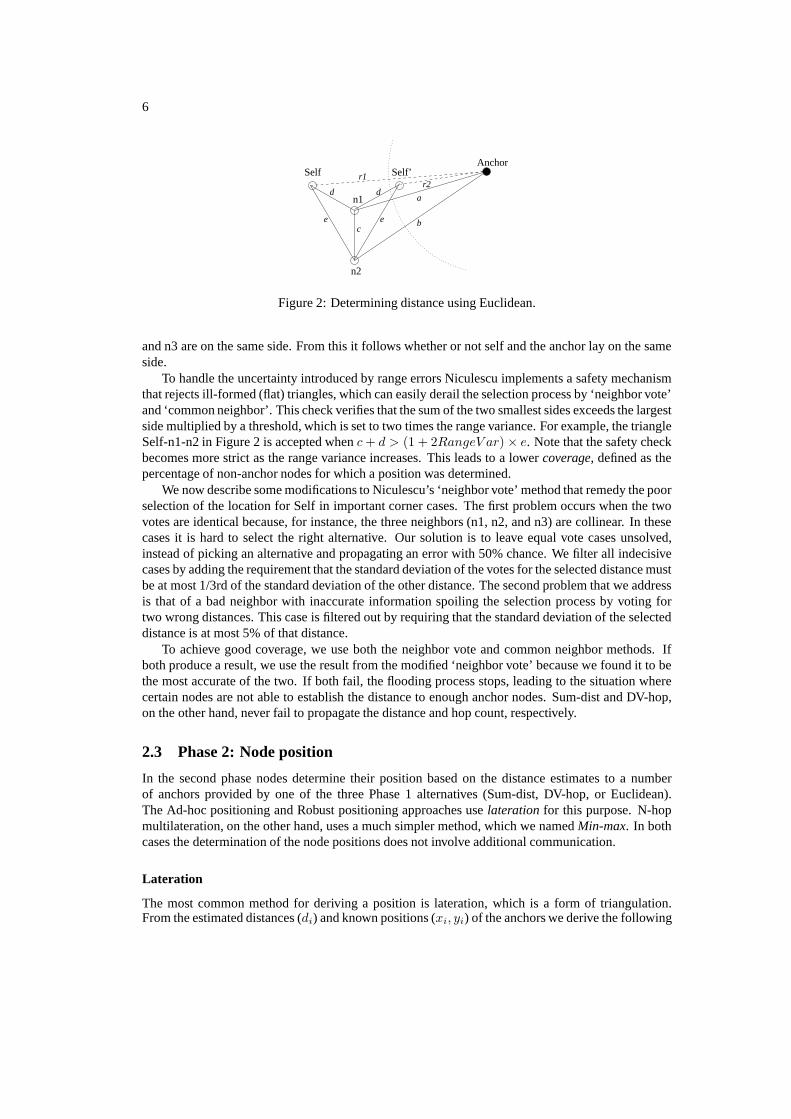
Lateration is quite expensive in the number of floating point operations that is required. A muchsimpler method is presented by Savvides et al. as part of the N-hop multilateration approach. Themain idea is to construct a bounding box for each anchor using its position and distance estimate,and then to determine the intersection of these boxes. The position of the node is set to the center ofthe intersection box. Figure 3 illustrates the Min-max method for a node with distance estimates tothree anchors. Note that the estimated position by Min-max is close to the true position computedthrough Lateration (i.e. the intersection of the three circles).
The bounding box of anchor a is created by adding and subtracting the estimated distance (da)from the anchor position (xa, ya):
[xa − da, ya − da] × [xa + da, ya + da].
8
pos.est.
Anchor2Anchor1
Anchor3
Figure 3: Determining position using Min-max.
The intersection of the bounding boxes is computed by taking the maximum of all coordinateminimums and the minimum of all maximums:
[max(xi − di), max(yi − di)] × [min(xi + di), min(yi + di)]
The final position is set to the average of both corner coordinates. As for Lateration, we only acceptthe final position if the residue is small.
2.4 Phase 3: Refinement
The objective of the third phase is to refine the (initial) node positions computed during Phase 2.These positions are not very accurate, even under good conditions (high connectivity, small rangeerrors), because not all available information is used in the first two phases. In particular, mostranges between neighboring nodes are neglected when the node-anchor distances are determined.The iterative Refinement procedure proposed by Savarese et al. [17] does take into account all inter-node ranges, when nodes update their positions in a small number of steps. At the beginning of eachstep a node broadcasts its position estimate, receives the positions and corresponding range estimatesfrom its neighbors, and performs the Lateration procedure of Phase 2 to determine its new position.In many cases the constraints imposed by the distances to the neighboring locations will force thenew position towards the true position of the node. When, after a number of iterations, the positionupdate becomes small, Refinement stops and reports the final position.
The basic iterative refinement procedure outlined above proved to be too simple to be used inpractice. The main problem is that errors propagate quickly through the network; a single errorintroduced by some node needs only d iterations to affect all nodes, where d is the network diameter.This effect was countered by 1) clipping undetermined nodes with non-overlapping paths to lessthan three anchors, 2) filtering out difficult symmetric topologies, and 3) associating a confidencemetric with each node and using them in a weighted least-squares solution (wAx = wb). Thedetails (see [17]) are beyond the scope of this paper, but the adjustments considerably improvedthe performance of the Refinement procedure. This is largely due to the confidence metric, whichallows filtering of bad nodes, thus increasing the (average) accuracy at the expense of coverage.
The N-hop multilateration approach by Savvides et al. [19] also includes an iterative refinementprocedure, but it is less sophisticated than the Refinement discussed above. In particular, theydo not use weights, but simply group nodes into so-called computation subtrees (over-constrained
9
configurations) and enforce nodes within a subtree to execute their position refinement in turn in afixed sequence to enhance convergence to a pre-specified tolerance. In the remainder of this paperwe will only consider the more advanced Refinement procedure of Savarese et al.
3 Simulation environment
To compare the three original distributed localization algorithms (Ad-hoc positioning, Robustpositioning, and N-hop multilateration) and to try out new combinations of phase 1, 2, and 3alternatives, we extended the simulator developed by Savarese et al. [17]. The underlying OMNeT++discrete event simulator [21] takes care of the semi-concurrent execution of the specific localizationalgorithm. Each sensor node ‘runs’ the same C++ code, which is parameterized to select a particularcombination of phase 1, 2, and 3 alternatives.
Our network layer supports localized broadcast only, and messages are simply delivered at theneighbors within a fixed radio range (circle) from the sending node; a more accurate model shouldtake radio propagation effects into account (see future work). Concurrent transmissions are allowed ifthe transmission areas (circles) do not overlap. If a node wants to broadcast a message while anothermessage in its area is in progress, it must wait until that transmission (and possibly other queuedmessages) are completed. In effect we employ a CSMA policy. Furthermore we do not considermessage corruption, so all messages sent during our simulation are delivered (after some delay).
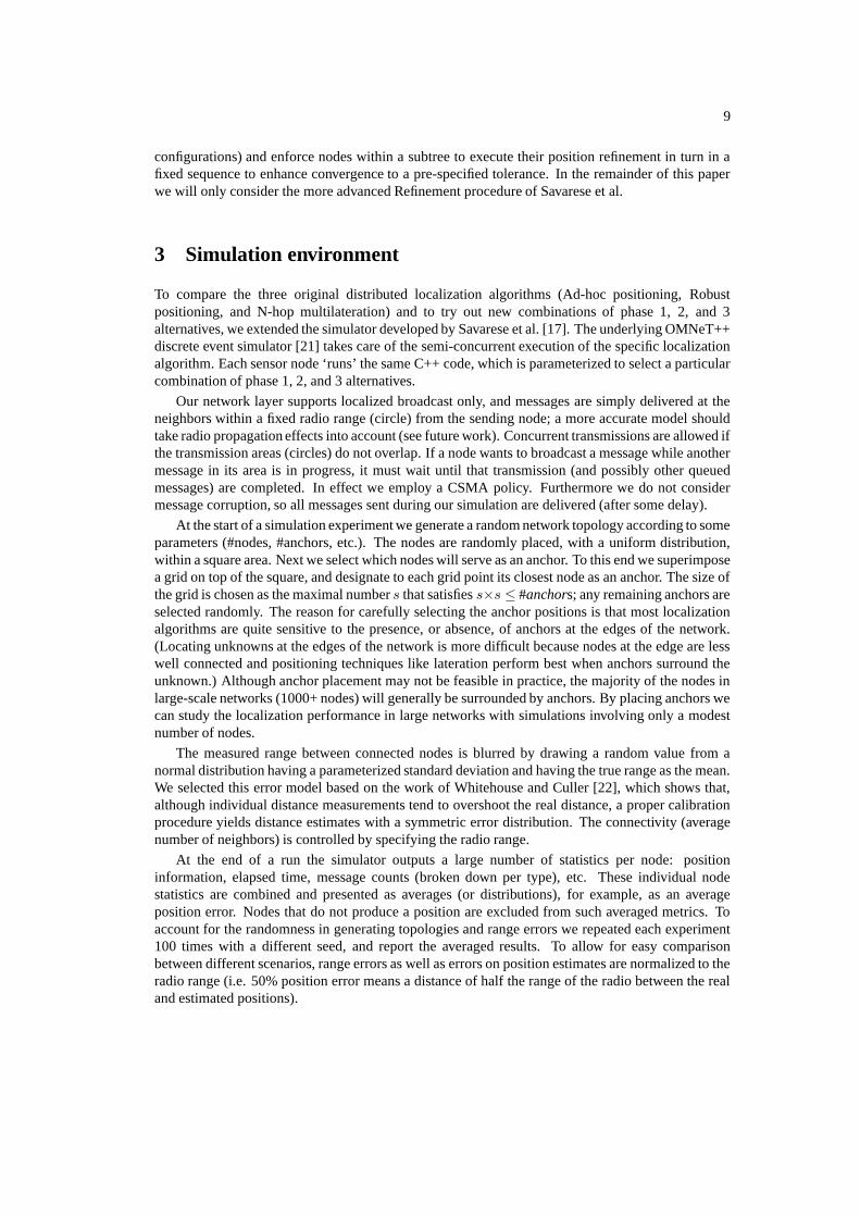
At the start of a simulation experiment we generate a random network topology according to someparameters (#nodes, #anchors, etc.). The nodes are randomly placed, with a uniform distribution,within a square area. Next we select which nodes will serve as an anchor. To this end we superimposea grid on top of the square, and designate to each grid point its closest node as an anchor. The size ofthe grid is chosen as the maximal number s that satisfies s×s ≤ #anchors; any remaining anchors areselected randomly. The reason for carefully selecting the anchor positions is that most localizationalgorithms are quite sensitive to the presence, or absence, of anchors at the edges of the network.(Locating unknowns at the edges of the network is more difficult because nodes at the edge are lesswell connected and positioning techniques like lateration perform best when anchors surround theunknown.) Although anchor placement may not be feasible in practice, the majority of the nodes inlarge-scale networks (1000+ nodes) will generally be surrounded by anchors. By placing anchors wecan study the localization performance in large networks with simulations involving only a modestnumber of nodes.
The measured range between connected nodes is blurred by drawing a random value from anormal distribution having a parameterized standard deviation and having the true range as the mean.We selected this error model based on the work of Whitehouse and Culler [22], which shows that,although individual distance measurements tend to overshoot the real distance, a proper calibrationprocedure yields distance estimates with a symmetric error distribution. The connectivity (averagenumber of neighbors) is controlled by specifying the radio range.
At the end of a run the simulator outputs a large number of statistics per node: positioninformation, elapsed time, message counts (broken down per type), etc. These individual nodestatistics are combined and presented as averages (or distributions), for example, as an averageposition error. Nodes that do not produce a position are excluded from such averaged metrics. Toaccount for the randomness in generating topologies and range errors we repeated each experiment100 times with a different seed, and report the averaged results. To allow for easy comparisonbetween different scenarios, range errors as well as errors on position estimates are normalized to theradio range (i.e. 50% position error means a distance of half the range of the radio between the realand estimated positions).
10
Standard scenario The experiments described in the subsequent sections share a standardscenario, in which certain parameters are varied: radio range (connectivity), anchor fraction, andrange errors. The standard scenario consists of a network of 225 nodes placed in a square with sidesof 100 units. The radio range is set to 14, resulting in an average connectivity of about 12. We use ananchor fraction of 5%, hence, 11 anchors in total, of which 9 (3×3) are placed in a grid-like position.The standard deviation of the range error is set to 10% of the radio range. The default flood limit forPhase 1 is set to 4 (Lateration requires a minimum of 3 anchors). Unless specified otherwise, all datawill be based on this standard scenario.
4 Results
In this section we present results for the first two phases (anchor distances and node positions).We study each phase separately and show how alternatives respond to different parameters. Theseintermediate results will be used in Section 5, where we will discuss the overall performance, andcompare complete localization algorithms. Throughout this section we will vary one parameter inthe standard scenario (radio range, anchor fraction, range error) at a time to study the sensitivity ofthe algorithms. The reader, however, should be aware that the three parameters are not orthogonal.
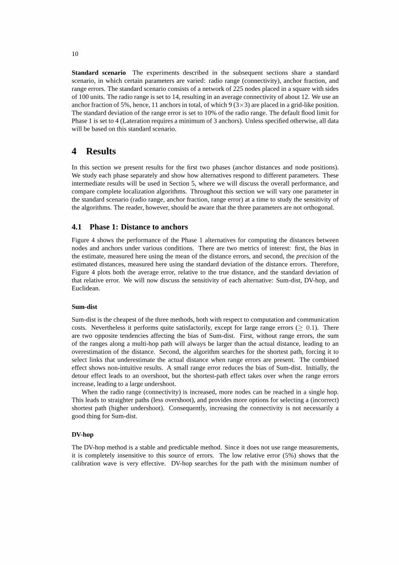
4.1 Phase 1: Distance to anchors
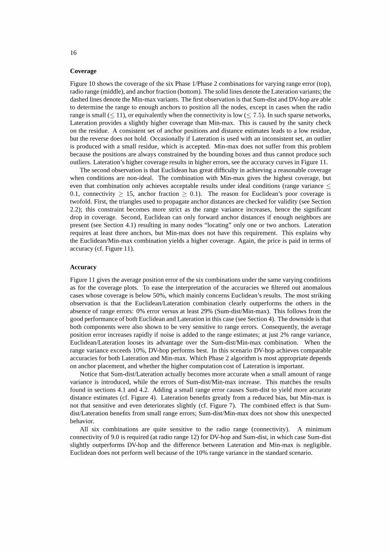
Figure 4 shows the performance of the Phase 1 alternatives for computing the distances betweennodes and anchors under various conditions. There are two metrics of interest: first, the bias inthe estimate, measured here using the mean of the distance errors, and second, the precision of theestimated distances, measured here using the standard deviation of the distance errors. Therefore,Figure 4 plots both the average error, relative to the true distance, and the standard deviation ofthat relative error. We will now discuss the sensitivity of each alternative: Sum-dist, DV-hop, andEuclidean.
Sum-dist
Sum-dist is the cheapest of the three methods, both with respect to computation and communicationcosts. Nevertheless it performs quite satisfactorily, except for large range errors (≥ 0.1). Thereare two opposite tendencies affecting the bias of Sum-dist. First, without range errors, the sumof the ranges along a multi-hop path will always be larger than the actual distance, leading to anoverestimation of the distance. Second, the algorithm searches for the shortest path, forcing it toselect links that underestimate the actual distance when range errors are present. The combinedeffect shows non-intuitive results. A small range error reduces the bias of Sum-dist. Initially, thedetour effect leads to an overshoot, but the shortest-path effect takes over when the range errorsincrease, leading to a large undershoot.
When the radio range (connectivity) is increased, more nodes can be reached in a single hop.This leads to straighter paths (less overshoot), and provides more options for selecting a (incorrect)shortest path (higher undershoot). Consequently, increasing the connectivity is not necessarily agood thing for Sum-dist.
DV-hop
The DV-hop method is a stable and predictable method. Since it does not use range measurements,it is completely insensitive to this source of errors. The low relative error (5%) shows that thecalibration wave is very effective. DV-hop searches for the path with the minimum number of
11
-0.4
-0.2
0
0.2
0.4
0.6
0.8
0 0.1 0.2 0.3 0.4 0.5R
elat
ive
dist
ance
err
or[x
act
ual d
ista
nce]
Range variance
DV-hopSum-dist
EuclideanMean
Std dev
-0.4
-0.2
0
0.2
0.4
0.6
0.8
8 (4.2)
9 10 (6.4)
11 12 (9.0)
13 14 (12.1)
15 16 (15.5)
Rel
ativ
e di
stan
ce e
rror
[x a
ctua
l dis
tanc
e]
Radio range (avg. connectivity)
DV-hopSum-dist
EuclideanMean
Std dev
-0.4
-0.2
0
0.2
0.4
0.6
0.8
0 0.05 0.1 0.15 0.2
Rel
ativ
e di
stan
ce e
rror
[x a
ctua
l dis
tanc
e]
Anchor fraction
DV-hopSum-dist
EuclideanMean
Std dev
Figure 4: Sensitivity of Phase 1 methods: distance error (solid lines) and standard deviation (dashedlines).
hops, causing the average hop distance to be close to the radio range. The last hop on the pathfrom an anchor to a node, however, is usually shorter than the radio range, which leads to a slightoverestimation of the node-anchor distance. This effect is more pronounced for short paths, hencethe increased error for larger radio ranges and higher anchor fractions (i.e. fewer hops).
Euclidean
Euclidean is capable of determining the exact anchor-node distances, but only in the absence ofrange errors and in highly connected networks. When these conditions are relaxed, Euclidean’sperformance rapidly degrades. The curves in Figure 4 show that Euclidean tends to underestimatethe distances. The reason is that the selection process is forced to choose between two options that
12
0
1
2
3
4
5
-1 -0.5 0 0.5 1P
roba
bilit
y de
nsity
Relative range error
EuclideanOracle
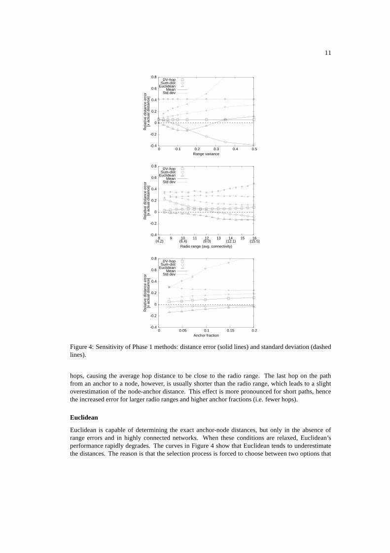
Figure 5: The impact of incorrect distance selection on Euclidean.
are quite far apart and that in many cases the shortest distance is incorrect. Consider Figure 2 again,where the shortest distance r2 falls within the radio range of the anchor. If r2 would be the correctdistance then the node should be in direct contact with the anchor avoiding the need for a selection.Therefore nodes simply have more chance to underestimate distances than to overestimate them inthe face of (small) range errors. This error can then propagate to nodes that are multiple hops awayfrom the anchor, causing them to underestimate the distance to the anchor as well.
We quantified the impact of the selection bias towards short distances. Figure 5 shows thedistribution of the errors, relative to the true distance, on the standard scenario for Euclidean’sselection mechanism (solid line) and an oracle that always selects the best distance (dashed line).The oracle’s distribution is nicely centered around zero (no error) with a sharp peak. Euclidean’sdistribution, in contrast, is skewed by a heavy tail at the left, signalling a bias for underestimations.
Euclidean’s sensitivity for connectivity is not immediately apparent from the accuracy data inFigure 4. The main effect of reducing the radio range is that Euclidean will not be able to propagatethe anchor distances. Recall that Euclidean’s selection methods require at least three neighbors witha distance estimate to advance the anchor distance one hop. In networks with low connectivity, twoparts connected only by a few links will often not be able to share anchors. This leads to problemsin Phase 2, where fewer node positions can be computed. The effects are quite pronounced, as willbecome clear in Section 5 (see the coverage curves in Figure 10).
4.2 Phase 2: Node position
To obtain insight into the fundamental behavior of the the Lateration and Min-max algorithms wenow report on some experiments with controlled distance errors and anchor placement. The impactof actual distance errors as produced by the Phase 1 methods will be discussed in Section 5.
Distance errors
Starting from the standard scenario we select for each node the five nearest anchors, and add somenoise to the real distances. This noise is generated by first taking a sample from a normal distributionwith the actual distance as the mean and a parameterized percentage of the distance as the standarddeviation. The result is then multiplied by a bias factor. The ranges for the standard deviation andbias factor follow from the Phase 1 measurements.
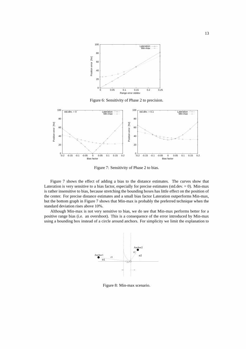
Figure 6 shows the sensitivity of Lateration and Min-max when the standard deviation percentagewas varied from 0 to 0.25, and the bias factor fixed at zero. Lateration outperforms Min-max forprecise distance estimates, but Min-max takes over for large standard deviations (≥ 0.15).
13
0
20
40
60
80
100
0 0.05 0.1 0.15 0.2 0.25P
ositi
on e
rror
[%
r]Range error stddev
LaterationMin-max
Figure 6: Sensitivity of Phase 2 to precision.
0
20
40
60
80
100
-0.2 -0.15 -0.1 -0.05 0 0.05 0.1 0.15 0.2
Pos
ition
err
or [
%r]
std.dev. = 0
Bias factor
LaterationMin-max
0
20
40
60
80
100
-0.2 -0.15 -0.1 -0.05 0 0.05 0.1 0.15 0.2
Pos
ition
err
or [
%r]
std.dev. = 0.1
Bias factor
LaterationMin-max
Figure 7: Sensitivity of Phase 2 to bias.
Figure 7 shows the effect of adding a bias to the distance estimates. The curves show thatLateration is very sensitive to a bias factor, especially for precise estimates (std.dev. = 0). Min-maxis rather insensitive to bias, because stretching the bounding boxes has little effect on the position ofthe center. For precise distance estimates and a small bias factor Lateration outperforms Min-max,but the bottom graph in Figure 7 shows that Min-max is probably the preferred technique when thestandard deviation rises above 10%.
Although Min-max is not very sensitive to bias, we do see that Min-max performs better for apositive range bias (i.e. an overshoot). This is a consequence of the error introduced by Min-maxusing a bounding box instead of a circle around anchors. For simplicity we limit the explanation to
Anchor1
Anchor2
r1α1
r2
α2
Figure 8: Min-max scenario.
14
Min-max
Anchor
Unknown
Estimated position
Lateration
Figure 9: Node locations computed for network topology of Figure 1.
the effects on the x-coordinate only. Figure 8 shows that Anchor1 making a small angle with thex-axis yields a tight bound (to the right), and that the large angle of Anchor2 yields a loose bound(to the left). The estimated position is off in the direction of the loose bound (to the left). Adding apositive bias to the range estimates causes the two bounds to shift proportionally. As a consequencethe center of the intersection moves into the direction of the bound with the longest range (to theright). Consequently the estimated coordinate moves closer to the true coordinate. The opposite willhappen if the anchor with the largest angle has the longest distance. Min-max selects the strongestbounds, leading to a preference for small angles and small distances, which favors the number of“good” cases where the coordinate moves closer to the true coordinate if a positive range bias isadded.
Anchor placement
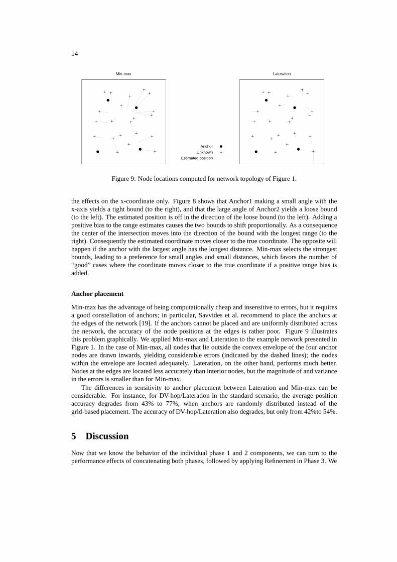
Min-max has the advantage of being computationally cheap and insensitive to errors, but it requiresa good constellation of anchors; in particular, Savvides et al. recommend to place the anchors atthe edges of the network [19]. If the anchors cannot be placed and are uniformly distributed acrossthe network, the accuracy of the node positions at the edges is rather poor. Figure 9 illustratesthis problem graphically. We applied Min-max and Lateration to the example network presented inFigure 1. In the case of Min-max, all nodes that lie outside the convex envelope of the four anchornodes are drawn inwards, yielding considerable errors (indicated by the dashed lines); the nodeswithin the envelope are located adequately. Lateration, on the other hand, performs much better.Nodes at the edges are located less accurately than interior nodes, but the magnitude of and variancein the errors is smaller than for Min-max.
The differences in sensitivity to anchor placement between Lateration and Min-max can beconsiderable. For instance, for DV-hop/Lateration in the standard scenario, the average positionaccuracy degrades from 43% to 77%, when anchors are randomly distributed instead of thegrid-based placement. The accuracy of DV-hop/Lateration also degrades, but only from 42%to 54%.
5 Discussion
Now that we know the behavior of the individual phase 1 and 2 components, we can turn to theperformance effects of concatenating both phases, followed by applying Refinement in Phase 3. We
15
0
20
40
60
80
100
0 0.1 0.2 0.3 0.4 0.5
Cov
erag
e [%
]
Range variance
DV-hopSum-dist
EuclideanLateration
Min-max
0
50
100
150
0 0.1 0.2 0.3 0.4 0.5
Pos
ition
err
or [
%r]
Range variance
DV-hopSum-dist
EuclideanLateration
Min-max
0
20
40
60
80
100
8 (4.2)
9 10 (6.4)
11 12 (9.0)
13 14 (12.1)
15 16 (15.5)
Cov
erag
e [%
]
Radio range (avg. connectivity)
DV-hopSum-dist
EuclideanLateration
Min-max
0
50
100
150
200
250
300
8 (4.2)
9 10 (6.4)
11 12 (9.0)
13 14 (12.1)
15 16 (15.5)
Pos
ition
err
or [
%r]
Radio range (avg. connectivity)
DV-hopSum-dist
EuclideanLateration
Min-max
0
20
40
60
80
100
0 0.05 0.1 0.15 0.2
Cov
erag
e [%
]
Anchor fraction
DV-hopSum-dist
EuclideanLateration
Min-max
Figure 10: Coverage of Phase 1/2 combina-tions.
0
50
100
150
0 0.05 0.1 0.15 0.2
Pos
ition
err
or [
%r]
Anchor fraction
DV-hopSum-dist
EuclideanLateration
Min-max
Figure 11: Accuracy of Phase 1/2 combina-tions.
will study the sensitivity of various combinations to connectivity, anchor fraction, and range errorsusing both the resulting position error and coverage.
5.1 Phases 1 and 2 combined
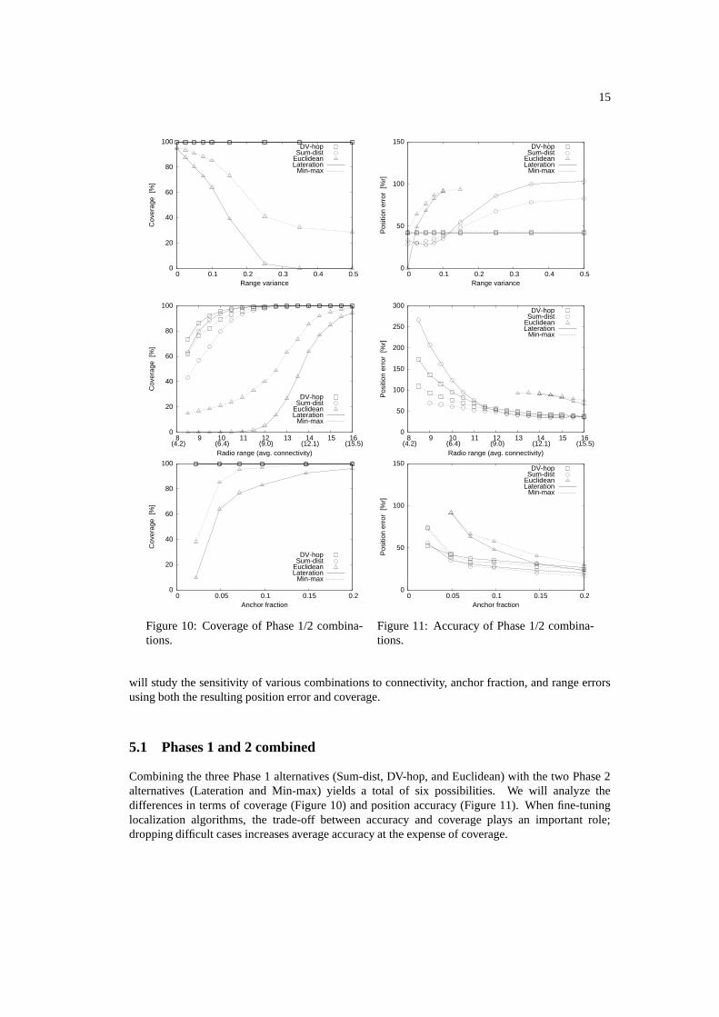
Combining the three Phase 1 alternatives (Sum-dist, DV-hop, and Euclidean) with the two Phase 2alternatives (Lateration and Min-max) yields a total of six possibilities. We will analyze thedifferences in terms of coverage (Figure 10) and position accuracy (Figure 11). When fine-tuninglocalization algorithms, the trade-off between accuracy and coverage plays an important role;dropping difficult cases increases average accuracy at the expense of coverage.
16
Coverage
Figure 10 shows the coverage of the six Phase 1/Phase 2 combinations for varying range error (top),radio range (middle), and anchor fraction (bottom). The solid lines denote the Lateration variants; thedashed lines denote the Min-max variants. The first observation is that Sum-dist and DV-hop are ableto determine the range to enough anchors to position all the nodes, except in cases when the radiorange is small (≤ 11), or equivalently when the connectivity is low (≤ 7.5). In such sparse networks,Lateration provides a slightly higher coverage than Min-max. This is caused by the sanity checkon the residue. A consistent set of anchor positions and distance estimates leads to a low residue,but the reverse does not hold. Occasionally if Lateration is used with an inconsistent set, an outlieris produced with a small residue, which is accepted. Min-max does not suffer from this problembecause the positions are always constrained by the bounding boxes and thus cannot produce suchoutliers. Lateration’s higher coverage results in higher errors, see the accuracy curves in Figure 11.
The second observation is that Euclidean has great difficulty in achieving a reasonable coveragewhen conditions are non-ideal. The combination with Min-max gives the highest coverage, buteven that combination only achieves acceptable results under ideal conditions (range variance ≤
0.1, connectivity ≥ 15, anchor fraction ≥ 0.1). The reason for Euclidean’s poor coverage istwofold. First, the triangles used to propagate anchor distances are checked for validity (see Section2.2); this constraint becomes more strict as the range variance increases, hence the significantdrop in coverage. Second, Euclidean can only forward anchor distances if enough neighbors arepresent (see Section 4.1) resulting in many nodes “locating” only one or two anchors. Laterationrequires at least three anchors, but Min-max does not have this requirement. This explains whythe Euclidean/Min-max combination yields a higher coverage. Again, the price is paid in terms ofaccuracy (cf. Figure 11).
Accuracy
Figure 11 gives the average position error of the six combinations under the same varying conditionsas for the coverage plots. To ease the interpretation of the accuracies we filtered out anomalouscases whose coverage is below 50%, which mainly concerns Euclidean’s results. The most strikingobservation is that the Euclidean/Lateration combination clearly outperforms the others in theabsence of range errors: 0% error versus at least 29% (Sum-dist/Min-max). This follows from thegood performance of both Euclidean and Lateration in this case (see Section 4). The downside is thatboth components were also shown to be very sensitive to range errors. Consequently, the averageposition error increases rapidly if noise is added to the range estimates; at just 2% range variance,Euclidean/Lateration looses its advantage over the Sum-dist/Min-max combination. When therange variance exceeds 10%, DV-hop performs best. In this scenario DV-hop achieves comparableaccuracies for both Lateration and Min-max. Which Phase 2 algorithm is most appropriate dependson anchor placement, and whether the higher computation cost of Lateration is important.
Notice that Sum-dist/Lateration actually becomes more accurate when a small amount of rangevariance is introduced, while the errors of Sum-dist/Min-max increase. This matches the resultsfound in sections 4.1 and 4.2. Adding a small range error causes Sum-dist to yield more accuratedistance estimates (cf. Figure 4). Lateration benefits greatly from a reduced bias, but Min-max isnot that sensitive and even deteriorates slightly (cf. Figure 7). The combined effect is that Sum-dist/Lateration benefits from small range errors; Sum-dist/Min-max does not show this unexpectedbehavior.
All six combinations are quite sensitive to the radio range (connectivity). A minimumconnectivity of 9.0 is required (at radio range 12) for DV-hop and Sum-dist, in which case Sum-distslightly outperforms DV-hop and the difference between Lateration and Min-max is negligible.Euclidean does not perform well because of the 10% range variance in the standard scenario.
17
0
20
40
60
80
100
0 0.1 0.2 0.3 0.4 0.5
Cov
erag
e [%
]
Range variance
DV-hop, LaterationSum-dist, Min-max
Euclidean, LaterationPhases 1 and 2 only
With Refinement
0
50
100
150
0 0.1 0.2 0.3 0.4 0.5
Pos
ition
err
or [
%r]
Range variance
DV-hop, LaterationSum-dist, Min-max
Euclidean, LaterationPhases 1 and 2 only
With Refinement
0
20
40
60
80
100
8 (4.2)
9 10 (6.4)
11 12 (9.0)
13 14 (12.1)
15 16 (15.5)
Cov
erag
e [%
]
Radio range (avg. connectivity)
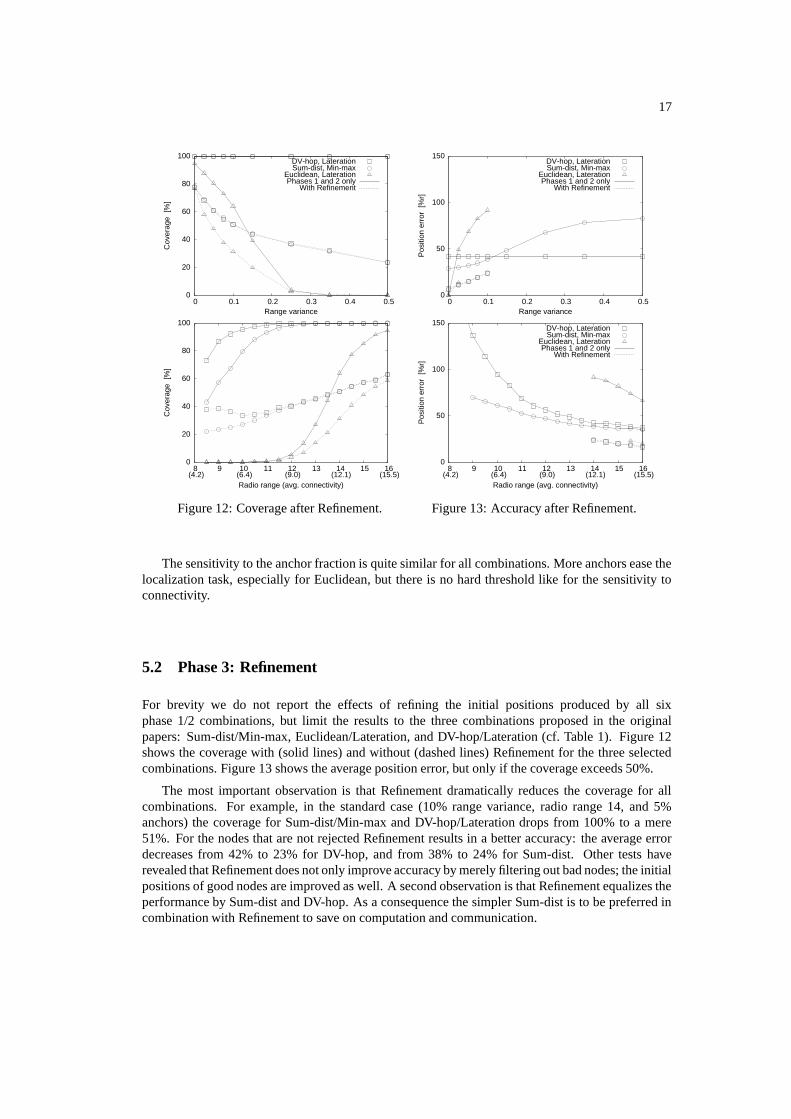
Figure 12: Coverage after Refinement.
0
50
100
150
8 (4.2)
9 10 (6.4)
11 12 (9.0)
13 14 (12.1)
15 16 (15.5)
Pos
ition
err
or [
%r]
Radio range (avg. connectivity)
DV-hop, LaterationSum-dist, Min-max
Euclidean, LaterationPhases 1 and 2 only
With Refinement
Figure 13: Accuracy after Refinement.
The sensitivity to the anchor fraction is quite similar for all combinations. More anchors ease thelocalization task, especially for Euclidean, but there is no hard threshold like for the sensitivity toconnectivity.
5.2 Phase 3: Refinement
For brevity we do not report the effects of refining the initial positions produced by all sixphase 1/2 combinations, but limit the results to the three combinations proposed in the originalpapers: Sum-dist/Min-max, Euclidean/Lateration, and DV-hop/Lateration (cf. Table 1). Figure 12shows the coverage with (solid lines) and without (dashed lines) Refinement for the three selectedcombinations. Figure 13 shows the average position error, but only if the coverage exceeds 50%.
The most important observation is that Refinement dramatically reduces the coverage for allcombinations. For example, in the standard case (10% range variance, radio range 14, and 5%anchors) the coverage for Sum-dist/Min-max and DV-hop/Lateration drops from 100% to a mere51%. For the nodes that are not rejected Refinement results in a better accuracy: the average errordecreases from 42% to 23% for DV-hop, and from 38% to 24% for Sum-dist. Other tests haverevealed that Refinement does not only improve accuracy by merely filtering out bad nodes; the initialpositions of good nodes are improved as well. A second observation is that Refinement equalizes theperformance by Sum-dist and DV-hop. As a consequence the simpler Sum-dist is to be preferred incombination with Refinement to save on computation and communication.
18
Table 2: Average number of messages per node.Type Sum-dist DV-hop Euclidean
Flood 4.3 2.2 3.5
Calibration - 2.6 -
Refinement 32 29 20
0
1
2
3
4
5
6
7
8
0 2 4 6 8 10
#Mes
sage
s pe
r no
de
Flood limit
DV-hop, LaterationSum-dist, Min-max
Euclidean, Lateration
0
50
100
150
0 2 4 6 8 10P
ositi
on e
rror
[%
r]Flood limit
DV-hop, LaterationSum-dist, Min-max
Euclidean, Lateration
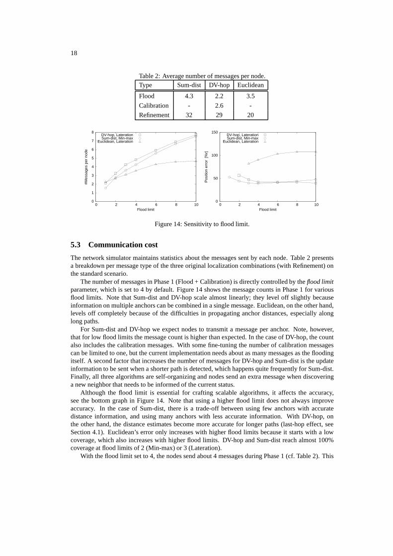
Figure 14: Sensitivity to flood limit.
5.3 Communication cost
The network simulator maintains statistics about the messages sent by each node. Table 2 presentsa breakdown per message type of the three original localization combinations (with Refinement) onthe standard scenario.
The number of messages in Phase 1 (Flood + Calibration) is directly controlled by the flood limitparameter, which is set to 4 by default. Figure 14 shows the message counts in Phase 1 for variousflood limits. Note that Sum-dist and DV-hop scale almost linearly; they level off slightly becauseinformation on multiple anchors can be combined in a single message. Euclidean, on the other hand,levels off completely because of the difficulties in propagating anchor distances, especially alonglong paths.
For Sum-dist and DV-hop we expect nodes to transmit a message per anchor. Note, however,that for low flood limits the message count is higher than expected. In the case of DV-hop, the countalso includes the calibration messages. With some fine-tuning the number of calibration messagescan be limited to one, but the current implementation needs about as many messages as the floodingitself. A second factor that increases the number of messages for DV-hop and Sum-dist is the updateinformation to be sent when a shorter path is detected, which happens quite frequently for Sum-dist.Finally, all three algorithms are self-organizing and nodes send an extra message when discoveringa new neighbor that needs to be informed of the current status.
Although the flood limit is essential for crafting scalable algorithms, it affects the accuracy,see the bottom graph in Figure 14. Note that using a higher flood limit does not always improveaccuracy. In the case of Sum-dist, there is a trade-off between using few anchors with accuratedistance information, and using many anchors with less accurate information. With DV-hop, onthe other hand, the distance estimates become more accurate for longer paths (last-hop effect, seeSection 4.1). Euclidean’s error only increases with higher flood limits because it starts with a lowcoverage, which also increases with higher flood limits. DV-hop and Sum-dist reach almost 100%coverage at flood limits of 2 (Min-max) or 3 (Lateration).
With the flood limit set to 4, the nodes send about 4 messages during Phase 1 (cf. Table 2). This
19
0
20
40
60
80
100
0 2 4 6 8 10
Cov
erag
e [%
]
Refinement limit
DV-hop, Lateration, RefinementSum-dist, Min-max, Refinement
Euclidean, Lateration, Refinement
0
20
40
60
80
100
0 2 4 6 8 10
Pos
ition
err
or [
%r]
Refinement limit
DV-Hop, Lateration, RefinementSum-dist, Min-max, Refinement
Euclidean, Lateration, Refinement
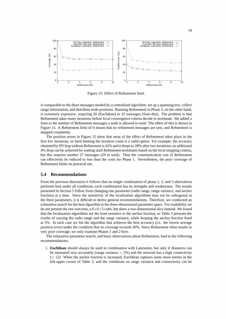
Figure 15: Effect of Refinement limit.
is comparable to the three messages needed by a centralized algorithm: set up a spanning tree, collectrange information, and distribute node positions. Running Refinement in Phase 3, on the other hand,is extremely expensive, requiring 20 (Euclidean) to 32 messages (Sum-dist). The problem is thatRefinement takes many iterations before local convergence criteria decide to terminate. We added alimit to the number of Refinement messages a node is allowed to send. The effect of this is shown inFigure 15. A Refinement limit of 0 means that no refinement messages are sent, and Refinement isskipped completely.
The position errors in Figure 15 show that most of the effect of Refinement takes place in thefirst few iterations, so hard limiting the iteration count is a valid option. For example, the accuracyobtained by DV-hop without Refinement is 42% and it drops to 28% after two iterations; an additional4% drop can be achieved by waiting until Refinement terminates based on the local stopping criteria,but this requires another 27 messages (29 in total). Thus the communication cost of Refinementcan effectively be reduced to less than the costs for Phase 1. Nevertheless, the poor coverage ofRefinement limits its practical use.
5.4 Recommendations
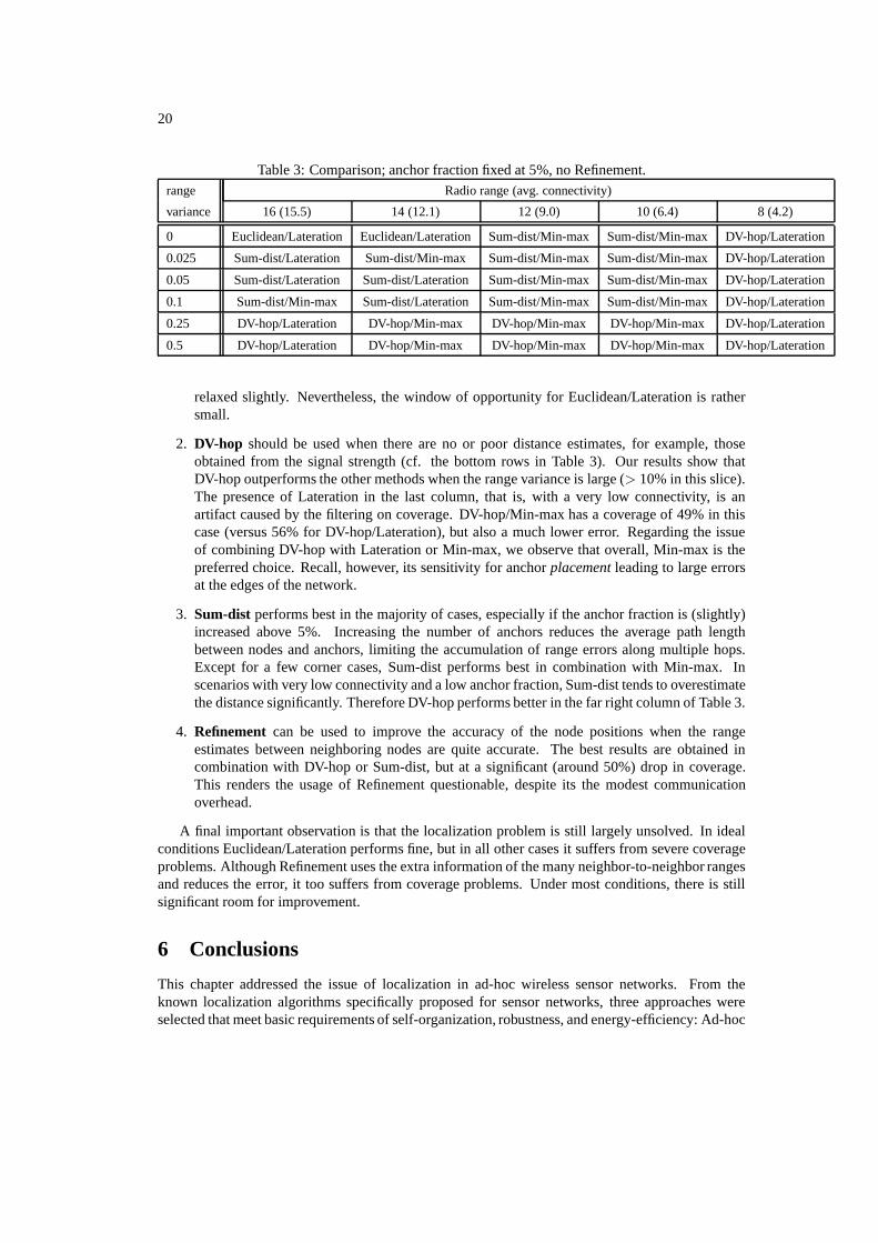
From the previous discussion it follows that no single combination of phase 1, 2, and 3 alternativesperforms best under all conditions; each combination has its strengths and weaknesses. The resultspresented in Section 5 follow from changing one parameter (radio range, range variance, and anchorfraction) at a time. Since the sensitivity of the localization algorithms may not be orthogonal inthe three parameters, it is difficult to derive general recommendations. Therefore, we conducted anexhaustive search for the best algorithm in the three-dimensional parameter space. For readability wedo not present the raw outcome, a 6×6×5 cube, but show a two-dimensional slice instead. We foundthat the localization algorithms are the least sensitive to the anchor fraction, so Table 3 presents theresults of varying the radio range and the range variance, while keeping the anchor fraction fixedat 5%. In each case we list the algorithm that achieves the best accuracy (i.e. the lowest averageposition error) under the condition that its coverage exceeds 50%. Since Refinement often results invery poor coverage, we only examine Phases 1 and 2 here.
The exhaustive parameter search, and basic observations about Refinement, lead to the followingrecommendations:
1. Euclidean should always be used in combination with Lateration, but only if distances canbe measured very accurately (range variance < 2%) and the network has a high connectivity(≥ 12). When the anchor fraction is increased, Euclidean captures some more entries in theleft-upper corner of Table 3, and the conditions on range variance and connectivity can be
20
Table 3: Comparison; anchor fraction fixed at 5%, no Refinement.range Radio range (avg. connectivity)
variance 16 (15.5) 14 (12.1) 12 (9.0) 10 (6.4) 8 (4.2)
0 Euclidean/Lateration Euclidean/Lateration Sum-dist/Min-max Sum-dist/Min-max DV-hop/Lateration
0.025 Sum-dist/Lateration Sum-dist/Min-max Sum-dist/Min-max Sum-dist/Min-max DV-hop/Lateration
0.05 Sum-dist/Lateration Sum-dist/Lateration Sum-dist/Min-max Sum-dist/Min-max DV-hop/Lateration
0.1 Sum-dist/Min-max Sum-dist/Lateration Sum-dist/Min-max Sum-dist/Min-max DV-hop/Lateration
0.25 DV-hop/Lateration DV-hop/Min-max DV-hop/Min-max DV-hop/Min-max DV-hop/Lateration
0.5 DV-hop/Lateration DV-hop/Min-max DV-hop/Min-max DV-hop/Min-max DV-hop/Lateration
relaxed slightly. Nevertheless, the window of opportunity for Euclidean/Lateration is rathersmall.
2. DV-hop should be used when there are no or poor distance estimates, for example, thoseobtained from the signal strength (cf. the bottom rows in Table 3). Our results show thatDV-hop outperforms the other methods when the range variance is large (> 10% in this slice).The presence of Lateration in the last column, that is, with a very low connectivity, is anartifact caused by the filtering on coverage. DV-hop/Min-max has a coverage of 49% in thiscase (versus 56% for DV-hop/Lateration), but also a much lower error. Regarding the issueof combining DV-hop with Lateration or Min-max, we observe that overall, Min-max is thepreferred choice. Recall, however, its sensitivity for anchor placement leading to large errorsat the edges of the network.
3. Sum-dist performs best in the majority of cases, especially if the anchor fraction is (slightly)increased above 5%. Increasing the number of anchors reduces the average path lengthbetween nodes and anchors, limiting the accumulation of range errors along multiple hops.Except for a few corner cases, Sum-dist performs best in combination with Min-max. Inscenarios with very low connectivity and a low anchor fraction, Sum-dist tends to overestimatethe distance significantly. Therefore DV-hop performs better in the far right column of Table 3.
4. Refinement can be used to improve the accuracy of the node positions when the rangeestimates between neighboring nodes are quite accurate. The best results are obtained incombination with DV-hop or Sum-dist, but at a significant (around 50%) drop in coverage.This renders the usage of Refinement questionable, despite its the modest communicationoverhead.
A final important observation is that the localization problem is still largely unsolved. In idealconditions Euclidean/Lateration performs fine, but in all other cases it suffers from severe coverageproblems. Although Refinement uses the extra information of the many neighbor-to-neighbor rangesand reduces the error, it too suffers from coverage problems. Under most conditions, there is stillsignificant room for improvement.
6 Conclusions
This chapter addressed the issue of localization in ad-hoc wireless sensor networks. From theknown localization algorithms specifically proposed for sensor networks, three approaches wereselected that meet basic requirements of self-organization, robustness, and energy-efficiency: Ad-hoc
21
positioning [14], Robust positioning [17], and N-hop multilateration [19]. Although these threealgorithms were developed independently, they share a common structure. We were able to identifya generic, 3-phase approach to determine the individual node positions consisting of the steps below:
1. Determine the distances between unknowns and anchor nodes.
2. Derive for each node a position from its anchor distances.
3. Refine the node positions using information about the range to, and positions of, neighboringnodes.
We studied three Phase 1 alternatives (Sum-dist, DV-hop, and Euclidean), two Phase 2 alternatives(Lateration and Min-max) and an optional Refinement procedure for Phase 3. To this end the discreteevent simulator developed by Savarese et al. [17] was extended to allow for the execution of anarbitrary combination of alternatives.
Section 4 dealt with Phase 1 and Phase 2 in isolation. For Phase 1 alternatives, we studied thesensitivity to range errors, connectivity, and fraction of anchor nodes (with known positions). DV-hopproved to be stable and predictable, Sum-dist and Euclidean showed tendencies to under estimate thedistances between anchors and unknowns. Euclidean was found to have difficulties in propagatingdistance information under non-ideal conditions, leading to low coverage in the majority of cases.The results for Phase 2 showed that Lateration is capable of obtaining very accurate positions, butalso that it is very sensitive to the accuracy and precision of the distance estimates. Min-max is morerobust, but is sensitive to the placement of anchors, especially at the edges of the network.
In Section 5 we compared all six phase 1/2 combinations under different conditions. No singlecombination performs best; which algorithm is to be preferred depends on the conditions (rangeerrors, connectivity, anchor fraction and placement). The Euclidean/Lateration combination [14]should be used only in the absence of range errors (variance < 2%) and requires a high node con-nectivity. The DV-hop/Min-max combination, which is a minor variation on the DV-hop/Laterationapproach proposed in [14] and [17], performs best when there are no or poor distance estimates,for example, those obtained from the signal strength. The Sum-dist/Min-max combination [19] isto be preferred in the majority of other conditions. The benefit of running Refinement in Phase 3 isconsidered to be questionable since in many cases the coverage dropped by 50%, while the accuracyonly improved significantly in the case of small range errors. The communication overhead ofRefinement was shown to be modest (2 messages per node) in comparison to the controlled floodingof Phase 1 (4 messages per node).
Future work Regarding the future, the ultimate distributed localization algorithm is yet to bedevised. Under ideal circumstances Euclidean/Lateration performs fine, but in all other cases thereis significant room for improvement. Furthermore, additional effort is needed to bridge the gapbetween simulations and real-world localization systems. For instance, we need to gather more dataon the actual behavior of sensor nodes, particularly with respect to physical effects like multipath,interference, and obstruction.
Acknowledgements
This work was first published in Elsevier Computer Networks [12]. We thank Elsevier for giving uspermission to reproduce the material. We also thank Andreas Savvides and Dragos Niculescu fortheir input and for sharing their code with us.
22
References
[1] I. Akyildiz, W. Su, Y. Sankarasubramaniam, and E. Cayirci. A survey on sensor networks. IEEE Commu-nications Magazine, 40(8):102–114, 2002.
[2] S. Atiya and G. Hager. Real-time vision-based robot localization. IEEE Trans. on Robotics and Automa-tion, 9(6):785–800, 1993.
[3] P. Bahl and V. Padmanabhan. RADAR: An in-building RF-based user location tracking system. In Info-com, volume 2, pages 575–584, Tel Aviv, Israel, March 2000.
[4] N. Bulusu, J. Heidemann, and D. Estrin. GPS-less low-cost outdoor localization for very small devices.IEEE Personal Communications, 7(5):28–34, October 2000.
[5] S. Capkun, M. Hamdi, and J.-P. Hubaux. GPS-free positioning in mobile ad-hoc networks. ClusterComputing, 5(2):157–167, April 2002.
[6] J. Chen, K. Yao, and R. Hudson. Source localization and beamforming. IEEE Signal Processing Magazin,19(2):30–39, 2002.
[7] L. Doherty, K. Pister, and L. El Ghaoui. Convex position estimation in wireless sensor networks. In IEEEInfocom 2001, Anchorage, AK, April 2001.
[8] L. Girod and D. Estrin. Robust range estimation using acoustic and multimodal sensing. In IEEE/RSJ Int.Conf. on Intelligent Robots and Systems (IROS), Maui, Hawaii, October 2001.
[9] T. He, C. Huang, B. M. Blum, J. A. Stankovic, and T. Abdelzaher. Range-free localization schemes forlarge scale sensor networks. In ACM International Conference on Mobile Computing and Networking(Mobicom), pages 81–95, San Diego, CA, September 2003.
[10] J. Hightower and G. Borriello. Location systems for ubiquitous computing. IEEE Computer, 34(8):57–66,August 2001.
[11] J. Hightower, R. Want, and G. Borriello. SpotON: An indoor 3D location sensing technology based onRF signal strength. UW CSE 00-02-02, University of Washington, Department of Computer Science andEngineering, Seattle, WA, February 2000.
[12] K. Langendoen and N. Reijers. Distributed localization in wireless sensor networks: a quantitative com-parison. Elsevier Computer Networks, 43:499–518, 2003.
[13] J. Leonard and H. Durrant-Whyte. Mobile robot localization by tracking geometric beacons. IEEE Trans.on Robotics and Automation, 7(3):376–382, 1991.
[14] D. Niculescu and B. Nath. Ad-hoc positioning system. In IEEE GlobeCom, November 2001.[15] N. Priyantha, A. Chakraborty, and H. Balakrishnan. The Cricket location-support system. In 6th ACM Int.
Conf. on Mobile Computing and Networking (Mobicom), pages 32–43, Boston, MA, August 2000.[16] V. Ramadurai and M. Sichitiu. Localization in wireless sensor networks: A probabilistic approach. In Int.
Conf. on Wireless Networks (ICWN), pages 275–281, Las Vegas, NV, June 2003.[17] C. Savarese, K. Langendoen, and J. Rabaey. Robust positioning algorithms for distributed ad-hoc wireless
sensor networks. In USENIX technical annual conference, pages 317–328, Monterey, CA, June 2002.[18] A. Savvides, C.-C. Han, and M. Srivastava. Dynamic fine-grained localization in ad-hoc networks of
sensors. In 7th ACM Int. Conf. on Mobile Computing and Networking (Mobicom), pages 166–179, Rome,Italy, July 2001.
[19] A. Savvides, H. Park, and M. Srivastava. The bits and flops of the n-hop multilateration primitive for nodelocalization problems. In First ACM Int. Workshop on Wireless Sensor Networks and Application (WSNA),pages 112–121, Atlanta, GA, September 2002.
[20] R. Tinos, L. Navarro-Serment, and C. Paredis. Fault tolerant localization for teams of distributed robots. InIEEE Int. Conf. on Intelligent Robots and Systems, volume 2, pages 1061–1066, Maui, HI, October 2001.
[21] A. Varga. The OMNeT++ discrete event simulation system. In European Simulation Multiconference(ESM’2001), Prague, Czech Republic, June 2001.
[22] K. Whitehouse and D. Culler. Callibration as parameter estimation in sensor networks. In First ACM Int.Workshop on Wireless Sensor Networks and Application (WSNA), pages 59–67, Atlanta, GA, September2002.
[23] Y. Xu, J. Heidemann, and D. Estrin. Geography-informed energy conservation for ad-hoc routing. In 7thACM International Conference on Mobile Computing and Networking (Mobicom), pages 70–84, Rome,Italy, 2001.
[24] J. Zhao and R. Govindan. Understanding Packet Delivery Performance In Dense Wireless Sensor Net-

23
works. In First Int. Conf. on Embedded Networked Sensor Systems (SenSys), pages 1–13, November 2003.