Embed Size (px)
Citation preview

Designing Localization Algorithms forWireless Sensor Networks: A Geometric
Approach
Thesis submitted in partial fulfillment of
the requirements for the degree of
Doctor of Philosophy
by
Kaushik Mondal
(Roll No. 09612305)
Under the Supervision of
Dr. Partha Sarathi Mandal
to the
Department of Mathematics
Indian Institute of Technology Guwahati
Guwahati - 781039, India
December 2014

TH-1358_09612305

CERTIFICATE
This is to certify that this thesis entitled “Designing Localization Algorithms for
Wireless Sensor Networks: A Geometric Approach” being submitted by Mr.
Kaushik Mondal to the Department of Mathematics, Indian Institute of Technology
Guwahati, is a record of bona fide research work under my supervision and is worthy
of consideration for the award of the degree of Doctor of Philosophy of the Institute.
The results contained in this thesis have not been submitted in part or full to any
other university or institute for the award of any degree or diploma.
Place: IIT Guwahati Dr. Partha Sarathi Mandal
Date: Department of Mathematics
Indian Institute of Technology Guwahati
Guwahati-781039, Assam, India
iii
TH-1358_09612305

TH-1358_09612305

ACKNOWLEDGEMENTS
First I want to acknowledge my father. Like him, I wanted to study Mathematics, do
PhD from an IIT and be a teacher. I feel I am in the right way. From my childhood,
my mother always taught me to be a good person at first which I will continue to try for
rest of my life. I convey my deepest gratitude to my parents for all their encouragements,
supports and inspirations not only during my PhD but throughout my life. I am also
grateful to my brother who is very close to my heart and understands me so well. My
love and blessings are always with him.
I met with Rima, my wife, in our graduating days and she became a part of my life
thereafter. She always encouraged me for higher studies knowing that we may have to
stay apart for a considerable amount of time. In between we got married and we have a
little son. She managed everything single handedly and never complained. I do not have
enough words to express my love for her.
I consider myself lucky to have Dr. Partha Sarathi Mandal as my supervisor. The
day, I met him first in his office, I can remember, he advised me to consult him without
any hesitation if I face any problem in this new place. From that very day I started to feel
that I have a guardian here as well. As days went by, love and respect continued to grow.
Manytimes, I felt that I was talking with my friend while discussing with him. Still, after
spending five and half years, I fear him more than a student fears a teacher. Apart from
academic lessons, I have learnt a lot from him which helped me to grow up in many ways.
I cannot remember the day when I first met “boudi”: (Dr. Debarati Mitra, Sir’s wife).
I found another very nice and down to earth person in her. You always find her with a
broad smile in her face. After a year of my joining, Barun, a good and responsible guy,
joined as a scholar under sir. I, Barun, sir and boudi often went out for dinner in the city
or had lunch at sir’s apartment as all of us are fond of good food. It gave me a feeling
of having a small family away from home. I enjoyed those days very much during this
memorable journey.
I remain grateful to sir for taking me as a PhD student knowing that I did not have any
knowledge in the field of Computer Science having done my bachelor and master degree
in Mathematics. He introduced me with the field of Computer Science, particularly with
Distributed Computing. Whenever I had problems, he gave me ample time to clear
v
TH-1358_09612305

my doubts. His proper guidance and invaluable advises towards my work helped me
immensely.
I want to thank Prof. Sukumar Nandi, Prof. Diganta Goswami and Dr. Kalpesh
Kapoor for their valuable inputs towards my work. I thank Prof. Bhabani K. Sinha, Prof.
Krishnendu Mukhopadhyaya of Indian Statistical Institute and Dr. Arindam Karmakar
of Tezpur University for giving their valuable suggestions for my work from their busy
schedules. All the comments, suggestions helped me a lot.
My sincere thanks goes to all my teachers of Visva Bharati University, specially Dr.
Anjan Kumar Bhuniya who often spent his valuable time for my study even outside office
hours. I extend my thanks to Anjan sir, Goutam sir, Srikanth sir, Rajen sir, Vinay sir,
Siddhartha sir, Pratyush sir and Sriparna madam who did not let me feel that even I have
not done any course under them. I express my sincere thanks to Sridhar da, Santanu da,
Phatik da and Pran da for helping me out in official and system related matters.
I cherished my stay in the institute largely due to my friends. I thank Arnab, Avijit
da, Mandar, Debopam, Kalyan, Kartoon, Manna, Murali, Santu, Abhisek, Anirban, Pur-
nendu da, Sahu da, Niladri da and many others for their encouragement and delightful
company. I thank Sandip for his help during my course work. I am specially thankful to
Himadri for his help in various matters. The list would be never ending. We read together
during course work, he helped me to learn writing codes, fixed the problems each time I
encountered with my laptop and thousands more.
I am deeply indebted to my school and university friends Sukanta, Saptarshi, Pratyush,
Falguni, Avijit, Rajib, Nikhil da, Sudipto da, Samiran da, Ramkrishna da, Biplab da and
others who always inspired me for research work.
The development of this dissertation would not have been possible without the finan-
cial support from the Council of Scientific and Industrial Research (CSIR), Government
of India. I would also like to thank the Indian Institute of Technology Guwahati for pro-
viding me a good academic environment and financial support during the last few months
of my research work.
Place: IIT Guwahati
Date: Kaushik Mondal
vi
TH-1358_09612305
ABSTRACT
Localization is one of the most important issues in wireless sensor networks. Localization
problems are more challenging when line-of-sight signals between anchors and sensors
are not available. We approach geometrically towards localization of static sensors based
on non-line-of-sight signals. Two range-based deterministic algorithms are proposed for
localization using static anchors. The first algorithm assumes presence of line-of-sight and
one-bound signals. Then we relax the assumption and propose another algorithm which
localizes sensors based on receiving unknown-bound signals.
Usually, large number of static anchors are required to localize all sensors in a network.
Measurement errors are unavoidable in range-based localization algorithms. To overcome
these problems, range-free localization algorithms using mobile anchors are proposed in
literature, where a mobile anchor localizes all static sensors traveling through the sensor
network. There are two different aspects of the existing algorithms. One aspect is to
improve localization accuracy whereas the other tries to reduce path lengths of mobile
anchors. The challenge is to design a movement strategy for mobile anchors which reduces
path length while meeting the requirements of a range-free technique that yields better
positioning accuracy. We propose a distributed range-free path planning algorithm for
mobile anchors to localize sensors in arbitrary connected network. Another path plan-
ning algorithm for mobile anchors is proposed to localize sensors in a rectangular region
with known boundary. The algorithms are designed in such a way that sensors can use
an existing range-free algorithm for better positioning accuracy. Both these algorithms
guarantee full localization.
In mobile wireless sensor networks, mobile sensors are needed to localize frequently un-
like the static sensors. Mobility of the sensors incur additional challenges for localization.
We propose a localization algorithm for mobile sensors assuming sensors do not change
direction during localization. An upper bound on localization error is ensured by this
algorithm. Then we relax the assumption and propose another algorithm which localizes
in presence of obstacles. Both algorithms are range-free, distributed and deterministic.
Each of our proposed algorithms in this thesis are compared with recent works to show
better performance.
vii
TH-1358_09612305

TH-1358_09612305
Contents
1 Introduction 1
1.1 Scope of the Thesis . . . . . . . . . . . . . . . . . . . . . . . . . . . . . . . 4
1.1.1 Localization in Presence of One-bound NLOS Signal . . . . . . . . 4
1.1.2 Analysis of Multiple-Bound Signals towards Localization . . . . . . 5
1.1.3 Mobile Sensor Localization using Static Anchor under Constrained
Motion . . . . . . . . . . . . . . . . . . . . . . . . . . . . . . . . . . 5
1.1.4 Mobile Sensor Localization in Presence of Obstacles . . . . . . . . . 6
1.1.5 Path Planning for Mobile Anchor in Connected Networks . . . . . . 6
1.1.6 Path Planning for Mobile Anchor in Rectangular Regions . . . . . . 6
2 Review of Related Works 7
2.1 Introduction . . . . . . . . . . . . . . . . . . . . . . . . . . . . . . . . . . . 7
2.2 Static Sensor Localization using Static Anchor . . . . . . . . . . . . . . . . 8
2.3 Static Sensor Localization using Mobile Anchor . . . . . . . . . . . . . . . 9
2.4 Mobile Sensor Localization . . . . . . . . . . . . . . . . . . . . . . . . . . . 11
3 Localization in Presence of One-bound NLOS Signal 15
3.1 Introduction . . . . . . . . . . . . . . . . . . . . . . . . . . . . . . . . . . . 15
3.1.1 Our contribution . . . . . . . . . . . . . . . . . . . . . . . . . . . . 15
3.2 Basic Idea . . . . . . . . . . . . . . . . . . . . . . . . . . . . . . . . . . . . 17
3.3 Positioning in Presence of Errors in Measurement . . . . . . . . . . . . . . 25
3.4 Proposed Localization Algorithm . . . . . . . . . . . . . . . . . . . . . . . 28
3.4.1 System model . . . . . . . . . . . . . . . . . . . . . . . . . . . . . . 28
3.4.2 The algorithm . . . . . . . . . . . . . . . . . . . . . . . . . . . . . . 29
ix
TH-1358_09612305
3.5 Simulation . . . . . . . . . . . . . . . . . . . . . . . . . . . . . . . . . . . . 30
3.5.1 Comparison with existing works . . . . . . . . . . . . . . . . . . . . 35
3.6 Localization in Three Dimension . . . . . . . . . . . . . . . . . . . . . . . . 36
3.7 Robust Localization in NLOS . . . . . . . . . . . . . . . . . . . . . . . . . 38
3.8 Conclusions . . . . . . . . . . . . . . . . . . . . . . . . . . . . . . . . . . . 40
4 Analysis of Multiple-Bound Signals towards Localization 41
4.1 Introduction . . . . . . . . . . . . . . . . . . . . . . . . . . . . . . . . . . . 41
4.1.1 Our contribution . . . . . . . . . . . . . . . . . . . . . . . . . . . . 41
4.2 Basic Idea . . . . . . . . . . . . . . . . . . . . . . . . . . . . . . . . . . . . 42
4.3 Analysis of Two-Bound Signal . . . . . . . . . . . . . . . . . . . . . . . . . 45
4.3.1 Area of presence for a two-Bound signal . . . . . . . . . . . . . . . 49
4.4 Analysis of Multiple-Bound Signal . . . . . . . . . . . . . . . . . . . . . . . 51
4.5 Area of Presence for an Unknown-Bound Signal . . . . . . . . . . . . . . . 55
4.6 Proposed Localization Algorithm . . . . . . . . . . . . . . . . . . . . . . . 57
4.6.1 System model . . . . . . . . . . . . . . . . . . . . . . . . . . . . . . 57
4.6.2 The algorithm . . . . . . . . . . . . . . . . . . . . . . . . . . . . . . 57
4.7 Simulation Results . . . . . . . . . . . . . . . . . . . . . . . . . . . . . . . 58
4.8 Conclusions . . . . . . . . . . . . . . . . . . . . . . . . . . . . . . . . . . . 62
5 Mobile Sensor Localization using Static Anchor under Constrained Mo-
tion 63
5.1 Introduction . . . . . . . . . . . . . . . . . . . . . . . . . . . . . . . . . . . 63
5.1.1 Our contribution . . . . . . . . . . . . . . . . . . . . . . . . . . . . 64
5.2 Localization without Change of Direction . . . . . . . . . . . . . . . . . . . 64
5.2.1 System model . . . . . . . . . . . . . . . . . . . . . . . . . . . . . . 64
5.2.2 Beacon list . . . . . . . . . . . . . . . . . . . . . . . . . . . . . . . . 66
5.2.3 Finding line of movement . . . . . . . . . . . . . . . . . . . . . . . 67
5.2.4 Error analysis . . . . . . . . . . . . . . . . . . . . . . . . . . . . . . 68
5.2.5 Error minimization . . . . . . . . . . . . . . . . . . . . . . . . . . . 76
5.2.6 Position calculation . . . . . . . . . . . . . . . . . . . . . . . . . . . 77
5.2.7 Algorithm for localization without change of direction . . . . . . . . 77
x
TH-1358_09612305
5.3 Localization without Change of Direction in Presence of Obstacles . . . . . 78
5.3.1 Position calculation in presence of obstacles . . . . . . . . . . . . . 82
5.3.2 Algorithm in presence of obstacles . . . . . . . . . . . . . . . . . . . 82
5.4 Simulation Results . . . . . . . . . . . . . . . . . . . . . . . . . . . . . . . 83
5.4.1 Simulation for LWCD . . . . . . . . . . . . . . . . . . . . . . . . . . 83
5.4.2 Simulation for LWCDPO . . . . . . . . . . . . . . . . . . . . . . . . 86
5.5 Conclusion . . . . . . . . . . . . . . . . . . . . . . . . . . . . . . . . . . . . 89
6 Mobile Sensor Localization in Presence of Obstacles 91
6.1 Introduction . . . . . . . . . . . . . . . . . . . . . . . . . . . . . . . . . . . 91
6.1.1 Our contribution . . . . . . . . . . . . . . . . . . . . . . . . . . . . 91
6.2 Localization with Change of Direction . . . . . . . . . . . . . . . . . . . . 92
6.2.1 Algorithm for localization with change of direction . . . . . . . . . 94
6.3 Localization in Presence of Obstacles . . . . . . . . . . . . . . . . . . . . . 96
6.3.1 Problems due to Obstacles . . . . . . . . . . . . . . . . . . . . . . . 96
6.3.2 System model in presence of obstacle . . . . . . . . . . . . . . . . . 97
6.3.3 Beacon point selection in presence of obstacles . . . . . . . . . . . . 98
6.3.4 Algorithm for localization with change of direction in presence of
obstacle . . . . . . . . . . . . . . . . . . . . . . . . . . . . . . . . . 102
6.4 Simulation Results . . . . . . . . . . . . . . . . . . . . . . . . . . . . . . . 103
6.4.1 Simulation for LCD . . . . . . . . . . . . . . . . . . . . . . . . . . . 103
6.4.2 Simulation for LPO . . . . . . . . . . . . . . . . . . . . . . . . . . . 107
6.5 Conclusion . . . . . . . . . . . . . . . . . . . . . . . . . . . . . . . . . . . . 112
7 Path Planning for Mobile Anchor in Connected Networks 113
7.1 Introduction . . . . . . . . . . . . . . . . . . . . . . . . . . . . . . . . . . . 113
7.1.1 Our contribution . . . . . . . . . . . . . . . . . . . . . . . . . . . . 114
7.2 Path Planning . . . . . . . . . . . . . . . . . . . . . . . . . . . . . . . . . . 114
7.3 Distributed Algorithm for Path Planning . . . . . . . . . . . . . . . . . . . 120
7.3.1 Correctness and complexity analysis . . . . . . . . . . . . . . . . . . 122
7.4 Effect of Irregular Radio Propagation . . . . . . . . . . . . . . . . . . . . . 123
7.5 Simulation Results . . . . . . . . . . . . . . . . . . . . . . . . . . . . . . . 124
xi
TH-1358_09612305

7.6 Conclusion . . . . . . . . . . . . . . . . . . . . . . . . . . . . . . . . . . . . 128
8 Path Planning for Mobile Anchor in Rectangular Regions 129
8.1 Introduction . . . . . . . . . . . . . . . . . . . . . . . . . . . . . . . . . . . 129
8.1.1 Our contribution . . . . . . . . . . . . . . . . . . . . . . . . . . . . 129
8.2 Path Planning for Rectangular Region . . . . . . . . . . . . . . . . . . . . 130
8.2.1 Comparison with existing schemes . . . . . . . . . . . . . . . . . . . 133
8.3 Simulation Results . . . . . . . . . . . . . . . . . . . . . . . . . . . . . . . 134
8.4 Conclusion . . . . . . . . . . . . . . . . . . . . . . . . . . . . . . . . . . . . 136
9 Conclusion 137
xii
TH-1358_09612305
Chapter 1
Introduction
A sensor is an autonomous device consisting of a small processor, a transceiver, a memory
unit, a power source and sensing units. It has a communication range to communicate
with neighboring sensors which are located within its communication circle. Once sensors
are deployed over a region of interest, they form a network. Sensors monitor physical
or environmental conditions like light, temperature, humidity, etc, [39] and cooperatively
send data through the network to a sink. Estimating position of a sensor in wireless sensor
networks (WSNs) is very crucial for many real-life applications since finding location of
data source in very important. Knowledge about position of sensors is the basic require-
ment for geometric routing and many position-based applications such as surveillance
environment monitoring, industrial monitoring, structural monitoring, real time tracking,
habitat monitoring [11, 21, 28] etc. The goal of localization is to estimate position of
each sensor as accurately as possible, depending on the requirements of underlying ap-
plications. Although GPS is one of the widely used technique for location discovery in
outdoor networks [31], from the point of view of accuracy, cost and energy preservation,
it is not always practical to equip each sensor with a GPS receiver. A sensor with its
known position is termed as anchor. Anchor broadcasts signals with its own position
which are received by sensors to estimate their position. Direct signals are termed as
line-of-sight (LOS) signals [4, 6, 10, 15, 20, 27, 35, 70], whereas non-line-of-sight (NLOS)
signals [14, 22, 43, 61, 66, 67, 68, 77, 82, 83] reflect and/or scatter by various obstacles
before reaching to the destination sensors. Signal which reflects once before reaching to
1
TH-1358_09612305
a sensor is defined as one-bound signal [68]. Similarly, multiple time reflected signals are
called as multiple-bound. Information from the received signals and known positions of the
anchors are used to localize rest of the sensors in a WSN. There exist many localization
algorithms [4, 6, 10, 15, 20, 46, 56, 62, 68, 75, 84, 92] by which sensors can compute their
positions. Generally localization algorithms are classified into two categories: range-based
[68] and range-free [75, 84]. Range-based algorithms need to estimate distance or angle
information for positioning sensors, while range-free techniques rely on connectivity infor-
mation between anchors and sensors. Usually range-based techniques give better accuracy
whereas range-free techniques are simpler and cost effective. Range-based techniques use
received signal strength indicator (RSSI) [20], time of arrival (TOA) [92], time difference
of arrival (TDOA) [26, 85] to measure distances and angle of arrival (AOA) [56, 86] to
measure angles. In TOA technique, time synchronization between anchor and sensor is
required to compute distance between them. But time synchronization in WSN is not
very easy to implement. To avoid time synchronization, round trip delay method is used
[71, 72]. Friis transmission equation [49] is used to measure distance between anchor
and sensor in RSSI method. TOA technique provides better distance estimations than
RSSI technique. Time difference of arrival is calculated in TDOA method for distance
calculation. Using AOA technique, a sensor calculates the angle of arrival of signal from
an anchor by using directional antennas or digital compass [56]. Range measurement
errors and absence of LOS signals affect localization accuracy in range-based techniques.
In range-free techniques, usually anchors broadcast beacon periodically with fixed time
period. Ideally communication area of any anchor is a circular disk in two dimension
plane with range of the anchor as its radius. However in practice, radio propagation is
usually not homogenous in all directions because of the presence of multi-path fading and
different path losses depending on the direction of propagation, which is termed as radio
propagation irregularity [78]. Due to irregular radio propagation, signal does not reach up
to the boundary of the circular disk at every direction which affects localization accuracy.
So accurate localization is a challenging problem.
Usually to localize a static sensor, three reference points are required. So for a large
network, several number of static anchors are needed for localization. This motivates
researchers to use mobile anchor so that it can move around the network while serving
2
TH-1358_09612305
as reference points to the sensors [46, 75, 84]. By using a mobile anchor, we can save
large number of anchors with deployment cost in the expense of the mobility of the
mobile anchor. So, path planning of the mobile anchor has become an important issue
in the area of localization. The path planning problem [13, 34, 36, 37, 47, 48, 59] can
be divided in two different types depending on the knowledge of the underlying topology
formed by the sensors and the area of sensor deployment. For the first type, information
like connectivity is used whereas boundary information of the network is known in the
second type. The objectives of path planning are reducing path length, providing good
localization accuracy and full localization.
Mobile wireless sensor networks (MWSNs) is a recent development of WSNs where
sensors have mobility depending on the applications. There are lots of applications [24]
of MWSNs in service industry, house keeping, wildlife tracking, pollution monitoring,
photon detection, shooter detection etc. In MWSN, mobile sensors are more powerful in
terms of energy because they need to localize themselves frequently than static sensors
where localizing a static sensor once is sufficient. Now a days, advanced mobile sensors
who can control their movement, for example, mobile actuated sensor [18, 23], are moti-
vating researchers to find accurate localization methods. Generally there are three phases
in a localization method, (1) coordination, (2) measurement or data gathering and (3)
computation. In MWSN, mobile sensors are used to record time stamps of events like
receiving beacons in the coordination phase. This technique is used in many localization
schemes [40]. Measurement phase is different for range-based and range-free algorithms.
Range-based algorithms [41, 54] depends on distant and angle measurements and gener-
ally produce better results than range-free. In this phase sensors gather information like
hop count [55] in range-free algorithms. In the computation phase, approximate position
of the sensors are determined using the gathered information. Dead reckoning’ [33, 89] is
a technique used in this phase for mobile sensor localization. In this technique the sen-
sor calculates current position using previous position, moving speed and time difference
between current time and the time when the position of the sensor was last updated.
Mobile sensor localization methods can be centralized [40, 41] as well as distributed [69].
Since mobility requires rapid and continuous localization, distributed algorithms are more
effective than the centralized algorithms. Based on mobility of anchors and sensors, it is
3
TH-1358_09612305
possible to classify localization algorithms into four categories: (1) static sensors using
static anchors, (2) mobile sensors using static anchors, (3) static sensors using mobile
anchors and (4) mobile sensors using mobile anchors. In this thesis, we look upon first
three categories of localization problems stated above.
1.1 Scope of the Thesis
In this thesis, we approach towards different kind of localization problems geometrically.
We propose range-based localization techniques for static sensors using static anchors in
absence of LOS signals under different assumptions. Then we propose range-free local-
ization techniques for mobile sensors using static anchors under different assumptions in
presence of obstacles. Finally, we look upon path planning problem for mobile anchor
towards range-free localization. Two range-free path planning algorithms are proposed
for mobile anchor to localize static sensors under different scenario. In this section we
briefly describe the problems with results of this thesis.
1.1.1 Localization in Presence of One-bound NLOS Signal
In chapter 3, we propose range-based localization algorithm for static sensors in presence
of one-bound NLOS signals using static anchors. We use round trip delay method during
TOA technique for distance estimation and AOA technique for angle measurement. We
prove that in presence of measurement errors, the sensor in question lies within a convex
hull. Simulation results show that positioning accuracy of our scheme in presence of
measurement errors is better than the existing localization algorithm [14]. Considering
only two NLOS signals from an anchor, when the maximum error in distance measurement
is 1 meter, we achieve about 40% reduction in the root mean square error (RMSE) in
positioning compared to the semi-definite programming (SDP) scheme [14], which uses
at least eight NLOS signals to localize a sensor. If we use more than two signals then
positioning error decreases. For robust localization anchor needs three reply signals from
a sensor via different paths in absence of measurement errors. Since only one anchor is
sufficient, this gives us an advantage particularly in dealing with the sparse networks.
4
TH-1358_09612305
1.1.2 Analysis of Multiple-Bound Signals towards Localization
Practically, a signal may reflect more than once before reaching to a sensor. In chapter 4,
we analyze multiple-bound signals to use unknown-bound NLOS signals for localization
of static sensors using static anchors based on range estimations. To the best of our
knowledge, there is no geometrical algorithms present in literature taking care of multiple-
bound signals to localize static sensors. This motivates us to approach geometrically
towards NLOS localization of static sensors. We use RSS technique in addition to TOA
and AOA to handle multiple-bound signals. If signal traverses d distance from an anchor
before reaching the sensor then possible locations of the sensor are always within a circle
of radius d centering at the anchor. Now using information of a received multiple-bound
signal, we are able compute a circle with radius less than d, where the sensor is bound
to reside. We propose a technique to localize sensor when it receives multiple-bound
signals and the number of bounds are unknown. In this case, only assumption is that the
maximum possible number of bounds in the system is known. Simulation results show
improvement over trilateration when sensor receives three unknown-bound signals from
different anchors.
1.1.3 Mobile Sensor Localization using Static Anchor under Con-
strained Motion
In chapter 5, we propose range-free localization algorithms for mobile sensors using static
anchors where mobile sensors do not change direction of movement during localization.
Under this assumption, our proposed algorithm LWCD localizes sensors within any prede-
fined error bound ε when it passes through communication circles of two different anchors.
As it passes through more communication circles, positioning error can be further reduced.
Simulation results of LWCD show around 75% improvement of the positioning error over
the existing algorithm [90] in presence of radio irregularity. When mobile sensor passes
through three and five more communication circles, 40% and 55% further reduction in
error has been shown respectively. According to our model, obstacles may lie in be-
tween anchor and sensors to block communication. In presence of obstacles our proposed
algorithm LWCDPO can localize mobile sensors within same error bound as LWCD.
5
TH-1358_09612305
1.1.4 Mobile Sensor Localization in Presence of Obstacles
In chapter 6, we propose range-free localization algorithm for mobile sensors using static
anchors where mobile sensors change direction during localization. Obstacles may present
any where in the network. Simulation results show 67% and 63% improvement of the po-
sitioning error over the existing algorithm [90] corresponding to two different selection
criteria in presence of radio irregularity. We propose a novel technique for obstacle detec-
tion and proposed another algorithm LPO which localizes sensors in presence of obstacles
with change of direction. It achieves 52% and 49% improvements corresponding to two
different selection criteria in terms of localization accuracy compared to [90] in presence
of radio irregularity.
1.1.5 Path Planning for Mobile Anchor in Connected Networks
In chapter 7, we consider path planning problem for mobile anchors in any arbitrary con-
nected network to localize static sensors. We propose a distributed range-free movement
strategy to localize all sensors within r/2 error-bound in a connected network, where r is
the transmission range of the sensors and the mobile anchor. To the best of our knowledge,
this is the first work where localization and path planning are done using connectivity
of the network without any range estimation. Simulation results show improvement over
existing work [48] in terms of both path length and localization accuracy.
1.1.6 Path Planning for Mobile Anchor in Rectangular Regions
In chapter 8, we propose path planning for mobile anchors in any rectangular region with
known boundary to localize static sensors. Theoretically we show that the length of the
path traversed by the anchor is lesser in the proposed hexagonal movement strategy com-
pared to other existing path planning methods [25, 34, 37, 59] for covering a rectangular
region. Simulation results support all theoretical results for path planning with localiza-
tion accuracy. Results show 7.35% to 27.74% improvement of our scheme over different
schemes in terms of path length while covering a bounded rectangular region.
6
TH-1358_09612305
Chapter 2
Review of Related Works
2.1 Introduction
Localization is one of the most important issues in WSNs and it is an widely studied
research area. Many localization algorithms [4, 6, 10, 15, 20, 46, 56, 62, 75, 84, 92] are there
in literature. Localization algorithms can be classified in different categories depending on
range estimation, mobility of sensors and anchors etc. Based on range estimation, there
are two categories; range-based [12, 15, 20, 27, 64, 70, 79, 80] and range-free [9, 30, 44, 55,
60, 81, 84]. Positioning using range-based algorithms are more accurate than range-free
ones. Usually for range estimation, TOA [20, 71], TDOA [15, 26], AOA [22, 54] and RSSI
[16] are used. To improve accuracy in range estimations, better range estimation tools
are designed. Few of the recent developments are listed below. Zhang et al. [91] proposed
a distributed angle estimation method for localization with multipath fading. Oberholzer
et al. proposed ultrasonic-based ranging platform, called SpiderBat [56] which is the first
ultrasonic-based sensor platform that can measure absolute angles between sensors within
an error of 5 degree. It is possible to estimate sensor’s position with a precision of the
order of a few centimeters with the help of measured angles. Srirangarajan et al. [74]
proposed a TOA based ranging technique which gives sub meter accuracy in distance
measurement. Here accuracy does not depend on the distance between the transmitter
and the receiver. Sinha et al. [72] used round trip delay method for distance measurement
using electromagnetic signal and showed that there is an error of 3 meter while measuring
7
TH-1358_09612305
a distance equal to 1.5 kilometer. On the other hand, range-free techniques rely on
connectivity information, hop-count etc. Hence range-free techniques are cost effective as
they do not need special hardware like range-based schemes. Localization algorithms are
divided into four categories based on mobility of anchors and sensors; (1) static sensors
using static anchors, (2) mobile sensors using static anchors, (3) static sensors using mobile
anchors and (4) mobile sensors using mobile anchors. According to this classification, we
present our literature study.
2.2 Static Sensor Localization using Static Anchor
Trilateration [70] is used for sensor localization when the distances between a sensor
and at least three anchors are known. It finds the intersection point of the three circles
centered at the anchors as the position of the sensor. Error in distance measurement
leads to an intersection area of those three circles instead of a point in the method of
trilateration. When the number of anchors are more than three, then multilateration
is used for positioning. Multilateration provides better accuracy than trilateration as
possible area of presence is less due to more number of reference points. Minimum mean
square error method (MMSE) [92] is used in multilateration which attempts to detect the
position of a sensor by minimizing the error using an objective function. In triangulation
technique, measured angles are used for positioning instead of distances. Patil et al. [62]
used circular triangulation. A time-based positioning scheme (TPS) [15] for outdoor is
proposed, which uses TDOA to detect location of the sensors. TPS is good in terms of
computation overhead and scalability. Bulusu et al. [9] proposed a localization algorithm
based on computing centroid of the proximate reference points using radio frequency
communications. Localization techniques proposed by AbdelSalam et al. [2, 3] used
AOA, RSSI technique and centroid method for localizing sensors using a single anchor.
Ortiz et al. [35] used trigonometric figures for sensor localization in a probabilistic model
and showed improvements over [9] in terms of positional accuracy. Sometimes sensors may
be under the control of some adversaries or some attackers. In that case after calculating
the position, verification is also required to ensure correct position of the sensor before
using the position for some applications. This is known as secure localization. Capkun
8
TH-1358_09612305
et al. proposed verifiable multilateration [10] for secure positioning using set of verifiers.
Delat et al. proposed a deterministic secure localization algorithm [20] based on RSSI
and TDOA techniques. Authors proved that six and four verifiers are sufficient to detect
a faking sensor using TDOA and RSSI technique respectively and hence provide stronger
results than [10]. In range-free techniques [6], information like hop counts, connectivity are
used. Sub-area localization (SAL) [4] is a range-free technique, where the central server
finds the correct sub-area and sets the center of mass of the sub-area as the sensor’s
position.
Localization becomes more challenging under NLOS scenario i.e., when LOS path is
not available. Ebrahimian and Scholtz [22] proposed a source localization scheme using
reflection, where direct and reflected signals are used. Here the sensors are equipped
with unidirectional antenna. Pahlavan et al. [61] proposed indoor geo-location in the
absence of direct path by mitigating NLOS ranging errors. Considering NLOS ranging
errors, Sinha et al. [73] proposed a technique which finds an area where a sensor is
bound to reside. Technique for refinement of area of presence of sensors is also given in
their scheme. Chen et al. [14] proposed a probabilistic NLOS sensor localization scheme
based on semi definite programming where NLOS localization problem is approximated
by a convex optimization problem using the SDP relaxation technique. In this paper
authors considered different cases depending on the prior knowledge of probabilities and
distributions of NLOS errors. We are intended to approach geometrically towards NLOS
localization problem in this thesis.
2.3 Static Sensor Localization using Mobile Anchor
Now we look at an overview of the existing static sensor localization schemes using mo-
bile anchor. A sphere-based localization algorithm [42] is proposed, which solves multiple
linear equations to estimate positions of sensors. A novel flying landmark localization
algorithm [60] is proposed, where anchor broadcasts its location information as it flies
through the sensing space. Then each unknown node in the sensing space estimates its
own location based on the basic geometry principles. Zhang et al. [92] proposed a secure
localization algorithm for static anchors. Chia-Ho-Ou et al. [17] proposed a localization
9
TH-1358_09612305
scheme using mobile anchors with directional antenna. Ssu et al. [75] proposed a localiza-
tion scheme, where the sensor’s position is estimated as the intersection of perpendicular
bisector of two computed chords. However this scheme suffers from short chord length
problem. Our proposed range-free deterministic localization algorithms for mobile sen-
sors are motivated by the strategy of beacon point selection used in [75]. Xiao et al. [84]
improved over that scheme using pre-arrival and post-departure points along with the
beacon points to localize a sensor. Later Lee et al. [46] used beacon distance more effec-
tively as another geometric constraint and proposed a more accurate localization scheme.
In all the three schemes [46, 75, 84], since static sensors receive beacons from mobile
anchors, sensors know the co-ordinates of the beacon points. Hence chord formed by two
beacon points is unique [75]. Similarly unique circular lamina with known equations of
the circles can be formed using a beacon point in [46]. All these schemes are range-free
and provides good positioning accuracy. To reduce energy consumption, it is also very
important to propose suitable movement strategy for mobile anchor so that path length
can be reduced. Below we discuss existing path planning algorithms for mobile anchor.
We can view the path planning problem in two different ways depending on the knowl-
edge of the area of sensor deployment and the underlying topology formed by the sensors.
Topology-based path planning, can be viewed as a graph traversal problem. Sensors have
information about their neighbors which they send to the mobile anchor for determining
the path. Li et al. [47] proposed two algorithms named breadth first and backtracking
greedy algorithms. Li et al. [48] proposed a depth first traversal scheme DREAMS to
localize the sensors. Both these works need range estimations. In DREAMS, mobile an-
chor first visits a sensor using random movement before performing depth-first traversal on
the network. An already visited localized sensor provides information to the anchor about
it’s next destination. Algorithm stops when anchor returns to the first sensor. During
depth-first traversal, anchor performs distance-based heuristic movement using received
signal strength from sensors. Kim et al. [36] proposed a path planning for randomly
deployed sensors using trilateration method for localization. An already localized sensor
becomes a reference point to help other sensors to find their position which reduces path
length but localization error may propagate. Chang et al. [13] proposed another path
planning algorithm of the mobile anchor, where localization are done using the scheme
10
TH-1358_09612305
proposed by Galstyan et al. [1] and mobile sensor calculates its trajectory by moving
around already localized sensors. Our aim is to propose a path planning algorithm which
can decide its trajectory without using any range estimation in a connected network. Us-
ing connectivity of the network, we discover neighbors of a sensor as well as localize it by
the scheme [46] using our proposed path planning algorithm.
Assuming known boundaries of a network, Scan, Doublescan and Hilbert schemes
are proposed by Koutsonikolas et al. [37]. They used the localization scheme [52]. Scan
covers the whole area uniformly where the mobile anchor travels in line segments along
X-axis (or Y -axis) keeping a fixed distance between two line segments. In Doublescan,
anchor moves along both X-axis and Y -axis, which improves localization accuracy in the
expense of traveled distance. Hilbert reduces both error and path length with compare
to the other two. Huang et al. [34] proposed two path planning schemes namely Circles
and S-curves. The authors propose a Gaussian-Markov algorithm [38] to optimize the
path length of mobile anchor. But Gaussian-Markov algorithm can not improve over the
above mentioned algorithms. Based on trilateration, Han et al. [25] proposed a path
planning scheme for a mobile anchor. Using RSSI technique, sensor measures distances
from three different non collinear points and finds its position. Chia-Ho-Ou et al. [59]
proposed a movement strategy of the anchor which helps sensors to localize with good
accuracy by reducing the short chord length problem of the scheme [75]. Another path
planning MAALRH [29] is proposed, but it produces largest path length compared to
other strategies while covering a rectangular region including the corner points using a
boundary compensation method named MAALRH BCM . Our aim is to propose a path
planning which minimizes the path length compared to the existing works in literature
and guarantee positioning of each sensor using scheme proposed by Lee et al. [46].
2.4 Mobile Sensor Localization
Algorithms for localizing static sensors can be applied for localizing mobile sensors, but
computation cost is more since repeated run of the algorithms is needed as the mobile
sensors change their position frequently. Tilak et al. [76] experimented how frequently
localization algorithms for static sensors need to be executed to localize mobile sensors
11
TH-1358_09612305
with an acceptable accuracy and energy consumption. Navstar global positioning system
[31] is the mostly used technique for localizing mobile sensors. Kostas et al. proposed a
range-based algorithm [8] for navigation of mobile robots. Datta et al. [19] proposed an
algorithm which can be used for both static and mobile sensor networks, where sensors
constructs polygon of presence and shrinks it using received information, while mobile
sensors dilate it before sending to its neighbors. Yu et al. [88] proposed an range based
mobile sensor localization algorithm, assuming that the mobile sensors are not always
moving in the network. A time based self-organizing localization algorithm [53] is pro-
posed, where trilateration is used for localization. Han et al. [27] propose anchor’s position
selection algorithm based on triangulation which shows that the unknown sensor’s local-
ization error is the least when three anchors form an equilateral triangle. In [32], authors
proposed ultrasonic-based localization system for mobile robot. Their proposed algorithm
provides sufficient accuracy in the positioning of a robot based on ultrasonic reflection.
An algorithm proposed [87], where mobile sensors predict their positions using recorded
beacon information by guessing a mobility pattern under a statistical model. Hu et al.
[33] adapted sequential Monte Carlo Localization (MCL) to localize mobile sensors. It
assumes that all the mobile sensors know their maximum speed. Also sampling efficiency
of MCL is low. Number of anchors should be high to achieve good localization accuracy
in this algorithm. Uchiyama et al. [77] proposed urban pedestrians localization (UPL)
algorithm for positioning mobile users in urban area. In this work authors consider known
positions of the obstacles and calculate the area of presence of mobile users with certain
degree of accuracy. UPL provides better localization accuracy compared to MCL [33].
Alikhani et al. [5] proposed iCCA-MAP algorithm and compared it with MCL. Later
Baggio et al. [7] proposed Monte Carlo localization Boxed (MCB), which improved on
MCL by using bounding box (called anchor box here). Sampling efficiency was improved
using bounding box by reducing the scope of the presence of the sensor. Zhang et al.
[90] proposed Weighted Monte Carlo Localization (WMCL), which improved over MCB
by reducing the size of bounding box constructed in MCB. This work is based on se-
quential Monte Carlo Localization [33]. WMCL uses two-hop beacon neighbors negative
effects along with estimated position information of sensor’s neighbors to further reduce
the size of the sensors bounding box. Hence WMCL has higher sampling efficiency than
12
TH-1358_09612305
MCB as well as MCL. WMCL also improves the localization accuracy by using estimated
position information of sensors. But WMCL has large communication cost. WMCL-A
and WMCL-B [90] reduce communication cost. However, average errors of WMCL-A
and WMCL-B are relatively high than WMCL. A range-free algorithm for mobile sensor
localization is proposed in [58] depending on beacon point selection. The idea of modi-
fying beacon point positions is good but in practice marking beacon points suffers from
mobility of both sensors and anchors. Localization schemes in [50, 57] localizes mobile
sensors based on recorded historical information by predicting coordinates of the mobile
sensor. There are also some range-free algorithms for localizing static sensors using mobile
anchors. Chia-Ho-Ou et al. [17] proposed a localization scheme using mobile anchors with
directional antenna. Authors proposed algorithms based on maximum likelihood estima-
tor in [57, 80] to locate mobile sensors. Venkatesh et al. proposed an algorithm [79] based
on constrained least square estimator for localization of mobile sensors. In [12], authors
used residual test to discard NLOS signals before localize mobile sensors. Schemes based
on statistical models are usually computationally complex. In [45], authors proposed an
indoor mobile sensor localization algorithm based on RSSI measurement using past signal
strength measurements. Miao et al. [51] proposed range-based geometric localization
algorithm considering NLOS signals. Seow et al. [68] proposed a localization algorithm
in presence of multiple-bound signals in the network. A statistical proximity test is used
to discard multiple-bound signals with a high degree of accuracy. Remaining LOS and
one-bound signals are used for sensor localization. Error can be accumulated in [68] since
the discarding technique relays on statistical proximity test. Our aim is to propose a
range-free localization algorithm for mobile sensors using static anchor.
13
TH-1358_09612305

TH-1358_09612305
Chapter 3
Localization in Presence of
One-bound NLOS Signal
3.1 Introduction
In presence of obstacles, LOS signals may get blocked. Then localization under NLOS
condition becomes quite challenging due to absence of LOS signals. In literature, there are
different NLOS mitigation and localization methods using statistical techniques. Our aim
is to localize sensors geometrically under NLOS condition using TOA and AOA ranging
techniques. In absence of LOS signal, reflected signals may reach to the sensors. It is
difficult to figure out how many times a signal reflects before reaching to a sensor. So under
NLOS condition, it is challenging to propose localization technique relying on geometry as
structure of the signal propagation path is difficult to obtain. In this chapter we propose a
localization algorithm imposing constraint on number of reflections/bounds, which helps
to view the problem as a geometric problem. Theoretically, in absence of measurement
errors, accurate positioning is possible for one-bound signal. Area of presence of sensors
is computed in presence of measurement errors.
3.1.1 Our contribution
In this chapter we propose a deterministic algorithm that calculates position of a sensor
using received beacons from an anchor. If a sensor unwillingly measures incorrect AOA of
15
TH-1358_09612305
a received signal and replies back with an unexpected delay then anchor can detect that
wrong angle information and time delay during localization. For robust localization an-
chor needs three reply signals from a sensor via different paths in absence of measurement
errors. According to our model, each beacon is reflected only once before reaching the des-
tination sensor and maximum possible angle and distance measurement errors are known.
Our scheme gives accurate positioning if there is no range measurement errors, whereas
considering measurement errors, positioning can only be done approximately. Simulation
results show that positioning accuracy of our scheme in presence of measurement errors
is better than the existing localization algorithm [14]. For the sake of comparison, we
introduce Gaussian noise with mean = 0 and standard deviation = 4 meter along with
measurement errors. Simulation results show that considering only two NLOS signals
from an anchor, when the maximum error in distance measurement is 1 meter, about
40% reduction in the root mean square error (RMSE) in positioning is achieved compared
to the semi-definite programming (SDP) scheme proposed in [14], which uses at least
eight NLOS signals to localize a sensor. If more than two signals are used then position-
ing error decreases. For example, if there are eight NLOS signals and the maximum error
in distance measurement is 6 meter, then the RMSE in positioning is reduced by about
74%.
Another good feature of our proposed approach is that in most of the earlier works
[4, 6, 10, 15, 20, 62, 92], usually three anchors are used to locate a sensor. But in our
approach, only one anchor is sufficient to calculate the position of a sensor. This gives
us an advantage particularly in dealing with the sparse networks, by having only a single
anchor, which can locate all other sensors in its range.
The rest of the chapter is organized as follows. The basic idea on which our proposed
approach is developed, are explained in section 3.2. Section 3.3 discusses about the
positioning in presence of distance and angle measurement errors. In section 3.4, we
present the system model and our proposed algorithm. The simulation results of our
algorithm considering errors in measurements are presented in section 3.5, along with
performance comparison with existing approach. In section 3.6, we show how the proposed
approach can be extended to localization in three dimension. Section 3.7 discusses about
how the anchor can detect wrong angle information or error in round trip delay while
16
TH-1358_09612305
localizing a sensor, assuming no errors in measurements. We conclude in section 3.8.
3.2 Basic Idea
Sensor with unique id are deployed on a two dimensional plane. There are some reflectors
and anchors in the same plane. The position of a sensor is calculated based on a chosen
coordinate system. The positions of the anchors are known and those can be identified
uniquely by their positions. An anchor broadcasts beacon along with its position. A
sensor may receive the beacon directly (LOS communication) or after a reflection from
some reflector. We assume that there can be at most one reflection in the path from any
anchor to another sensor. One sensor may, however, receive more than one beacons from
different anchors. After receiving a beacon from an anchor, a sensor transmits back the
signal in the same direction from which it received the beacon (the angle of arrival with
respect to the common coordinate system being measured by AOA technique). After
receiving those beacons, the anchors also use TOA and AOA techniques to calculate the
round-trip time of arrival and angle of arrival with respect to the same coordinates system
for the same sensor. We show later that with the help of those angles of arrival and the
distances calculated from the TOA technique, it is possible for the anchors to find the
exact position of a sensor.
The connection between the geometry of Fig. 3.1 used in the following Lemma 3.2.1
and our localization problem is the following: S is considered as an anchor as well as
its position, P is the point of reflection on a reflector and Q is considered as a sensor as
well as its position, which is to be computed. The sensor Q receives the beacon from S
through the path SQ via P , after one reflection at P . We now state the following result:
Lemma 3.2.1. Consider a fixed point S on a straight line l with gradient ml. Let L be
the set of all parallel straight lines with gradient mL such that ml 6= mL. Let Pi be the
point of intersections of l with a line `i ∈ L, for i = 1, 2, · · · (Ref. Fig. 3.1). Let Qis be
the points on `i such that SPi + PiQi = d, for i = 1, 2, · · · , where d is a fixed distance.
Then all the Qis must lie on a straight line.
Proof. Without loss of generality, let the fixed point S on the straight line l be the origin
17
TH-1358_09612305
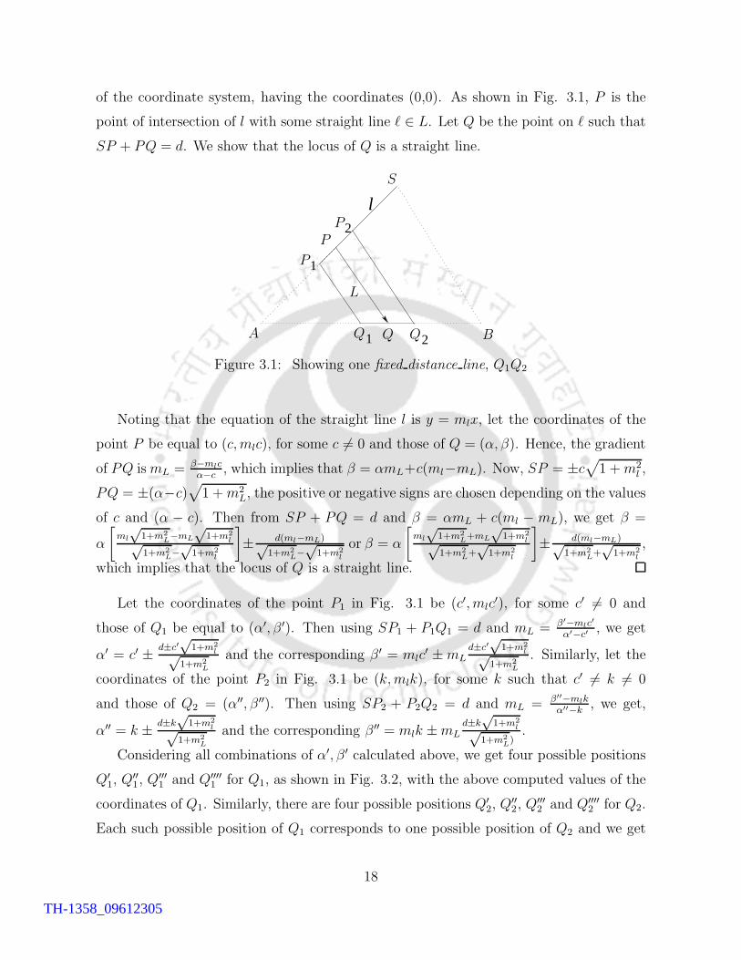
of the coordinate system, having the coordinates (0,0). As shown in Fig. 3.1, P is the
point of intersection of l with some straight line ` ∈ L. Let Q be the point on ` such that
SP + PQ = d. We show that the locus of Q is a straight line.
21
1
2
l
S
PP
P
L
QQQA B
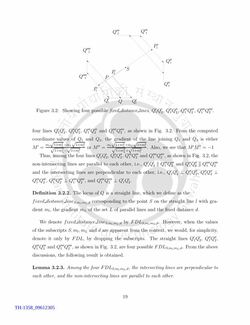
Figure 3.1: Showing one fixed distance line, Q1Q2
Noting that the equation of the straight line l is y = mlx, let the coordinates of the
point P be equal to (c,mlc), for some c 6= 0 and those of Q = (α, β). Hence, the gradient
of PQ ismL = β−mlcα−c
, which implies that β = αmL+c(ml−mL). Now, SP = ±c√
1 +m2l ,
PQ = ±(α−c)√
1 +m2L, the positive or negative signs are chosen depending on the values
of c and (α − c). Then from SP + PQ = d and β = αmL + c(ml − mL), we get β =
α
[
ml
√1+m2
L−mL
√1+m2
l√1+m2
L−√
1+m2l
]
± d(ml−mL)√1+m2
L−√
1+m2l
or β = α
[
ml
√1+m2
L+mL
√1+m2
l√1+m2
L+√
1+m2l
]
± d(ml−mL)√1+m2
L+√
1+m2l
,
which implies that the locus of Q is a straight line.
Let the coordinates of the point P1 in Fig. 3.1 be (c′, mlc′), for some c′ 6= 0 and
those of Q1 be equal to (α′, β ′). Then using SP1 + P1Q1 = d and mL = β′−mlc′
α′−c′, we get
α′ = c′ ± d±c′√
1+m2l√
1+m2L
and the corresponding β ′ = mlc′ ±mL
d±c′√
1+m2l√
1+m2L
. Similarly, let the
coordinates of the point P2 in Fig. 3.1 be (k,mlk), for some k such that c′ 6= k 6= 0
and those of Q2 = (α′′, β ′′). Then using SP2 + P2Q2 = d and mL = β′′−mlkα′′−k
, we get,
α′′ = k ± d±k√
1+m2l√
1+m2L
and the corresponding β ′′ = mlk ±mLd±k
√1+m2
l√1+m2
L).
Considering all combinations of α′, β ′ calculated above, we get four possible positions
Q′1, Q
′′1, Q
′′′1 and Q′′′′
1 for Q1, as shown in Fig. 3.2, with the above computed values of the
coordinates of Q1. Similarly, there are four possible positions Q′2, Q
′′2, Q
′′′2 and Q′′′′
2 for Q2.
Each such possible position of Q1 corresponds to one possible position of Q2 and we get
18
TH-1358_09612305
1
1
12
2
1
2
1 2
1
2
S
P
P
P
P ′
Q Q′Q′
Q′′
Q′′
Q′′′ Q′′′
Q′′′′
Q′′′′
Figure 3.2: Showing four possible fixed distance lines, Q′1Q
′2, Q
′′1Q
′′2, Q
′′′1 Q
′′′2 , Q
′′′′1 Q′′′′
2 .
four lines Q′1Q
′2, Q
′′1Q
′′2, Q
′′′1 Q
′′′2 and Q′′′′
1 Q′′′′2 , as shown in Fig. 3.2. From the computed
coordinate values of Q1 and Q2, the gradient of the line joining Q1 and Q2 is either
M ′ =ml
√1+m2
L−mL
√1+m2
l√1+m2
L−√
1+m2l
or M ′′ =ml
√1+m2
L+mL
√1+m2
l√1+m2
L+√
1+m2l
. Also, we see that M ′M ′′ = −1
Thus, among the four lines Q′1Q
′2, Q
′′1Q
′′2, Q
′′′1 Q
′′′2 and Q′′′′
1 Q′′′′2 , as shown in Fig. 3.2, the
non-intersecting lines are parallel to each other, i.e., Q′1Q
′2 ‖ Q′′′
1 Q′′′2 and Q′′
1Q′′2 ‖ Q′′′′
1 Q′′′′2
and the intersecting lines are perpendicular to each other, i.e., Q′1Q
′2 ⊥ Q′′
1Q′′2, Q
′′1Q
′′2 ⊥
Q′′′1 Q
′′′2 , Q
′′′1 Q
′′′2 ⊥ Q′′′′
1 Q′′′′2 , and Q′′′′
1 Q′′′′2 ⊥ Q′
1Q′2.
Definition 3.2.2. The locus of Q is a straight line, which we define as the
fixed distance lineS,ml,mL,d corresponding to the point S on the straight line l with gra-
dient ml, the gradient mL of the set L of parallel lines and the fixed distance d.
We denote fixed distance lineS,ml,mL,d by FDLS,ml,mL,d. However, when the values
of the subscripts S,ml, mL and d are apparent from the context, we would, for simplicity,
denote it only by FDL, by dropping the subscripts. The straight lines Q′1Q
′2, Q
′′1Q
′′2,
Q′′′1 Q
′′′2 and Q′′′′
1 Q′′′′2 , as shown in Fig. 3.2, are four possible FDLS,ml,mL,d. From the above
discussions, the following result is obtained.
Lemma 3.2.3. Among the four FDLS,ml,mL,d, the intersecting lines are perpendicular to
each other, and the non-intersecting lines are parallel to each other.
19
TH-1358_09612305
Lemma 3.2.4. A bisector of one of the angles between the straight lines l and any line
belonging to L is parallel to the FDLS,ml,mL,d.
Proof. It follows that gradients of the angular bisectors of the angles between l and any
line ∈ L are(ml
√1+m2
L−mL
√1+m2
l)
(√
1+m2L−√
1+m2l)
and(ml
√1+m2
L+mL
√1+m2
l)
(√
1+m2L+√
1+m2l)
. According to Lemma 3.2.1,
these are possible gradients of the FDLS,ml,mL,d.
Lemma 3.2.5. The position of a sensor cannot be uniquely identified if and only if the
sensor receives two beacons from the same anchor which are reflected from two parallel
reflectors.
Proof. First, we examine the characteristics of a pair of beacons, received by a sensor from
an anchor. As shown in the Fig. 3.3, S is the anchor, Q is the actual position of the sensor.
Q receives beacons from S through P1 and P2, where P1 and P2 are the two points of
reflection. Let ∠P1QX ′ = θ1, ∠P2QX ′ = θ2, (all the angles are measured counterclockwise
with respect to the positive X-axis), SP1 + P1Q = d1 and SP2 + P2Q = d2. By virtue of
TOA and AOA measurements, all of these parameters, i.e., θ1, θ2, d1 and d2 are known
to S (the exact details of finding the values of these four parameters are explained later
in this section).
In Fig. 3.3, we show another arbitrarily chosen point P ′1 on the line SP1 of gradient,
say, ml and another point Q′ such that ∠P ′1Q
′X ′′ = θ1 and SP ′1+P ′
1Q′ = d1. This implies
that the point Q′ is on the FDLS,ml,mL,d1 where mL is the gradient of the line P1Q. That
means, line QQ′ itself is the FDLS,ml,mL,d1.
Similarly, if we find another point P ′2 on the line SP2 having gradient, say, m′
l such that
∠P ′2Q
′X ′′ = θ2 and SP ′2 + P ′
2Q′ = d2, then the line QQ′ will also be the FDLS,m′
l,m′
L,d2 ,
where m′L is the gradient of the line P2Q. Now we have problems in uniquely identifying
the position of the sensor from the signals reflected from P1 and P2, as the solutions for
the possible position of Q in this case are infinitely many (corresponding to the line QQ′).
We note that under such a situation, according to Lemma 3.2.4, QQ′ is parallel to the
bisectors of both the angles ∠SP1Q and ∠SP2Q. Hence, the two reflectors are parallel to
each other.
Conversely, assume that there are two parallel reflectors. Two beacons from an anchor
reflected from those two parallel reflectors reach a sensor. Hence, the bisectors of the
20
TH-1358_09612305
12
1
2
2
21
1θ
θθ
θ
S
PP
P ′
P ′
QQ′
X
X ′
X ′′
Figure 3.3: Showing infinite many solutions for the position of a sensor along the lineQQ′
angles formed at the points of reflections are parallel. According to Lemma 3.2.4, the
FDLs corresponding to these two reflected paths have the same gradient, i.e., the possible
solutions for the position of the sensor are on a line.
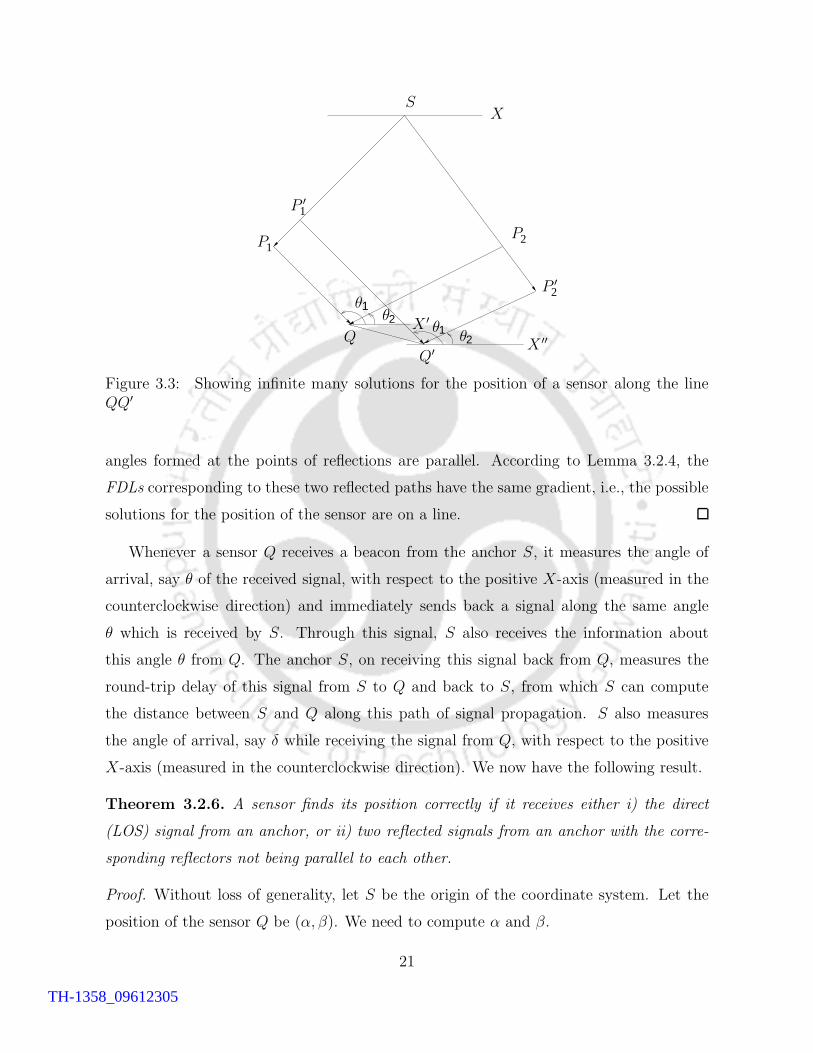
Whenever a sensor Q receives a beacon from the anchor S, it measures the angle of
arrival, say θ of the received signal, with respect to the positive X-axis (measured in the
counterclockwise direction) and immediately sends back a signal along the same angle
θ which is received by S. Through this signal, S also receives the information about
this angle θ from Q. The anchor S, on receiving this signal back from Q, measures the
round-trip delay of this signal from S to Q and back to S, from which S can compute
the distance between S and Q along this path of signal propagation. S also measures
the angle of arrival, say δ while receiving the signal from Q, with respect to the positive
X-axis (measured in the counterclockwise direction). We now have the following result.
Theorem 3.2.6. A sensor finds its position correctly if it receives either i) the direct
(LOS) signal from an anchor, or ii) two reflected signals from an anchor with the corre-
sponding reflectors not being parallel to each other.
Proof. Without loss of generality, let S be the origin of the coordinate system. Let the
position of the sensor Q be (α, β). We need to compute α and β.
21
TH-1358_09612305
1
1
1δ
δ − π
θ
S
Q
Q′
X
X ′
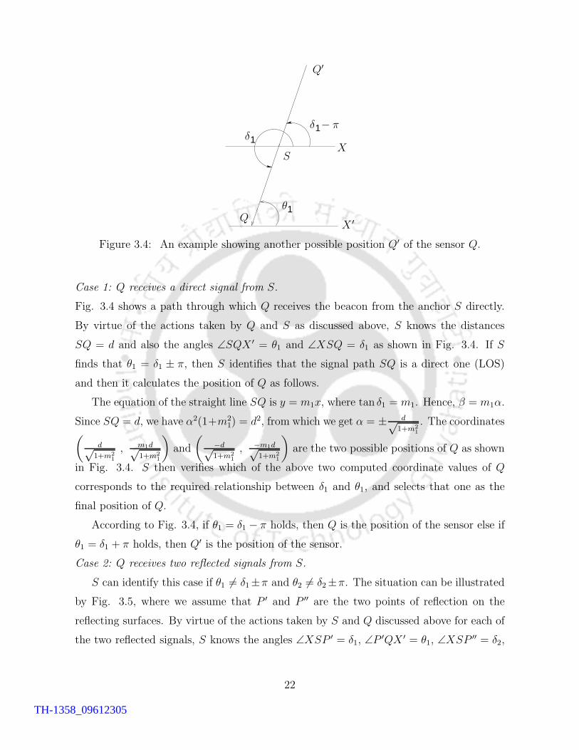
Figure 3.4: An example showing another possible position Q′ of the sensor Q.
Case 1: Q receives a direct signal from S.
Fig. 3.4 shows a path through which Q receives the beacon from the anchor S directly.
By virtue of the actions taken by Q and S as discussed above, S knows the distances
SQ = d and also the angles ∠SQX ′ = θ1 and ∠XSQ = δ1 as shown in Fig. 3.4. If S
finds that θ1 = δ1 ± π, then S identifies that the signal path SQ is a direct one (LOS)
and then it calculates the position of Q as follows.
The equation of the straight line SQ is y = m1x, where tan δ1 = m1. Hence, β = m1α.
Since SQ = d, we have α2(1+m21) = d2, from which we get α = ± d√
1+m21
. The coordinates(
d√1+m2
1
, m1d√1+m2
1
)
and
(
−d√1+m2
1
, −m1d√1+m2
1
)
are the two possible positions of Q as shown
in Fig. 3.4. S then verifies which of the above two computed coordinate values of Q
corresponds to the required relationship between δ1 and θ1, and selects that one as the
final position of Q.
According to Fig. 3.4, if θ1 = δ1 − π holds, then Q is the position of the sensor else if
θ1 = δ1 + π holds, then Q′ is the position of the sensor.
Case 2: Q receives two reflected signals from S.
S can identify this case if θ1 6= δ1±π and θ2 6= δ2±π. The situation can be illustrated
by Fig. 3.5, where we assume that P ′ and P ′′ are the two points of reflection on the
reflecting surfaces. By virtue of the actions taken by S and Q discussed above for each of
the two reflected signals, S knows the angles ∠XSP ′ = δ1, ∠P′QX ′ = θ1, ∠XSP ′′ = δ2,
22
TH-1358_09612305
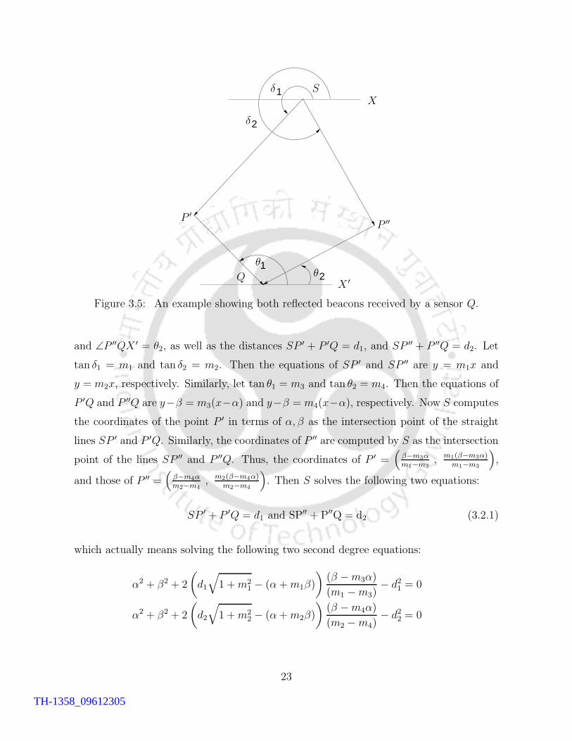
2
1
2 1θ
θ
δ
δ S
Q
P ′P ′′
X
X ′
Figure 3.5: An example showing both reflected beacons received by a sensor Q.
and ∠P ′′QX ′ = θ2, as well as the distances SP ′ + P ′Q = d1, and SP ′′ + P ′′Q = d2. Let
tan δ1 = m1 and tan δ2 = m2. Then the equations of SP ′ and SP ′′ are y = m1x and
y = m2x, respectively. Similarly, let tan θ1 = m3 and tan θ2 = m4. Then the equations of
P ′Q and P ′′Q are y−β = m3(x−α) and y−β = m4(x−α), respectively. Now S computes
the coordinates of the point P ′ in terms of α, β as the intersection point of the straight
lines SP ′ and P ′Q. Similarly, the coordinates of P ′′ are computed by S as the intersection
point of the lines SP ′′ and P ′′Q. Thus, the coordinates of P ′ =(
β−m3αm1−m3
, m1(β−m3α)m1−m3
)
,
and those of P ′′ =(
β−m4αm2−m4
, m2(β−m4α)m2−m4
)
. Then S solves the following two equations:
SP ′ + P ′Q = d1 and SP′′ + P′′Q = d2 (3.2.1)
which actually means solving the following two second degree equations:
α2 + β2 + 2
(
d1
√
1 +m21 − (α+m1β)
)
(β −m3α)
(m1 −m3)− d21 = 0
α2 + β2 + 2
(
d2
√
1 +m22 − (α+m2β)
)
(β −m4α)
(m2 −m4)− d22 = 0
23
TH-1358_09612305
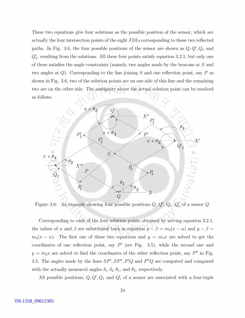
These two equations give four solutions as the possible position of the sensor, which are
actually the four intersection points of the eight FDLs corresponding to these two reflected
paths. In Fig. 3.6, the four possible positions of the sensor are shown as Q,Q′, Q1 and
Q′1, resulting from the solutions. All these four points satisfy equation 3.2.1, but only one
of these satisfies the angle constraints (namely, two angles made by the beacons at S and
two angles at Q). Corresponding to the line joining S and one reflection point, say P as
shown in Fig. 3.6, two of the solution points are on one side of this line and the remaining
two are on the other side. The ambiguity about the actual solution point can be resolved
as follows.
1
1
23
1
2
2
2
2
1
1
23
1
11
π + θ
π + θ
π + θ
π + θ
θ
θ
θ
θ
S
PP
P
P
P ′
P ′
P ′
P ′
Q
Q
Q′
Q′
X
X ′
X ′′
X ′′′
Figure 3.6: An example showing four possible positions Q, Q′, Q1, Q′1 of a sensor Q.
Corresponding to each of the four solution points obtained by solving equation 3.2.1,
the values of α and β are substituted back in equation y − β = m3(x − α) and y − β =
m4(x − α). The first one of these two equations and y = m1x are solved to get the
coordinates of one reflection point, say P ′ (see Fig. 3.5), while the second one and
y = m2x are solved to find the coordinates of the other reflection point, say P ′′ in Fig.
3.5. The angles made by the lines SP ′, SP ′′, P ′Q and P ′′Q are computed and compared
with the actually measured angles δ1, δ2, θ1, and θ2, respectively.
All possible positions, Q,Q′, Q1 and Q′1 of a sensor are associated with a four-tuple
24
TH-1358_09612305
(δ′, δ′′, θ′, θ′′), where δ′, δ′′, θ′, θ′′ are the angles made at S and at the sensor respectively
by both the signals with respect to the positive X-axis. According to Fig. 3.6, the
correct position of the sensor is either Q(δ1, δ2, θ1, θ2) or Q′(δ1−π, δ2−π, θ1+π, θ2+π) or
Q1(δ1, δ2−π, θ1+π, θ2) or Q′1(δ1−π, δ2, θ1, θ2+π). As anchor S has the information about
all the four angles made by the signals, it can choose the correct position of the sensor by
matching those known angles with the four-tuples of those four possible positions.
3.3 Positioning in Presence of Errors in Measure-
ment
In a practical situation, there are some errors in measuring angles and distances using AOA
and TOA techniques. Let ∆α and ∆β be the possible errors in finding the coordinates α
and β respectively of a sensor resulting due to such errors in measurement. To obtain the
expressions for these errors ∆α and ∆β in terms of the errors ∆m and ∆d in measuring
the gradient m and distance d respectively, we use the results in Lemma 3.2.1 to evaluate
α and β, instead of the two quadratic equations as in equation 3.2.1. From Lemma 3.2.1,
the locus of the sensor Q is the line AB which intersects with the two straight lines of
gradients m1 and m3 passing through the anchor S at the points A and B respectively.
Exact coordinates of A and B are calculated using angles measured by AOA technique.
We thus get two equations as given in equation 3.3.1 solving which the values of α and β
can be obtained.
(
√
1 +m21 −
√
1 +m23
)
β −(
m3
√
1 +m21 −m1
√
1 +m23
)
α+ d1(m3 −m1) = 0(
√
1 +m22 −
√
1 +m24
)
β −(
m4
√
1 +m22 −m2
√
1 +m24
)
α+ d2(m4 −m2) = 0
(3.3.1)
To find the effect of errors in measuring angles and distances, first differentiate the above
two equations in equation 3.3.1 with respect to m1, m2, m3, m4, d1, d2. Then to maximize
the errors ∆α and ∆β due to the error in measuring the angles, put ∆m1 = −∆m3 = ∆m
and ∆m2 = −∆m4 = ∆m. Also, we assume that ∆di = ∆d for i = 1, 2. Differentiating
the first equation in equation 3.3.1, we get the following:
p∆α + q∆β = r∆m+ s∆d (3.3.2)
25
TH-1358_09612305
where, p = m1
√
1 +m23 −m3
√
1 +m21, q =
√
1 +m21 −
√
1 +m23,
r =
(
m1√1+m2
1
− m3√1+m2
3
)
β −(
m1m3√1+m2
1
+ m1m3
sqrt1+m23
−√
1 +m21 −
√
1 +m23
)
α and
s = m3 −m1.
Similarly differentiating the second equation in equation 3.3.1, we get
p′∆α + q′∆β = r′∆m+ s′∆d (3.3.3)
where, p′ = m2
√
1 +m24 −m4
√
1 +m22, q
′ =√
1 +m22 −
√
1 +m24,
r′ =
(
m2√1+m2
2
− m4√1+m2
4
)
β −(
m2m4√1+m2
2
+ m2m4
sqrt1+m24
−√
1 +m22 −
√
1 +m24
)
α and
s′ = m4 −m2.
Solving equation 3.3.2 and equation 3.3.3 for ∆α and ∆β, we get the following:
∆α
∆β
=1
pq′ − qp′
q′ −q
−p′ p
r s
r′ s′
∆m
∆d
(3.3.4)
From the above equation 3.3.4, one can calculate maximum positioning error ∆α and
∆β using multi-variable optimization technique.
Again, through a different approach, however, for each received signal, erroneous mea-
surements of angles and distances lead us to an area instead of a line segment, where the
sensor is bound to reside. To find that area, we state the following theorem which is based
on the assumption that the values of the maximum possible errors in measuring distances
and angles are a priori known to the anchor. This assumption is justified because of the
results reported in [56, 63].
Theorem 3.3.1. On a two-dimensional plane, in presence of errors in measuring the
angles and distances, the anchor can locate any sensor within a convex hull containing the
sensor, if the values of the maximum possible errors in measuring distances and angles
are known.
Proof. Let the maximum possible errors in angle measurement and distance measurement
be φ and w, respectively. In Fig. 3.7, the line QX ′ is drawn parallel to the line SX . Let
the error-free angles at the anchor S and the sensor Q corresponding to a one-bound
signal be δ(= ∠XSP ) and θ(= ∠PQX ′) respectively. Due to the measurement error,
26
TH-1358_09612305
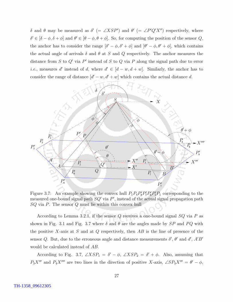
δ and θ may be measured as δ′ (= ∠XSP ′) and θ′ (= ∠P ′Q′X ′′) respectively, where
δ′ ∈ [δ − φ, δ + φ] and θ′ ∈ [θ − φ, θ + φ]. So, for computing the position of the sensor Q,
the anchor has to consider the range [δ′ − φ, δ′ + φ] and [θ′ − φ, θ′ + φ], which contains
the actual angle of arrivals δ and θ at S and Q respectively. The anchor measures the
distance from S to Q′ via P ′ instead of S to Q via P along the signal path due to error
i.e., measures d′ instead of d, where d′ ∈ [d − w, d + w]. Similarly, the anchor has to
consider the range of distance [d′ − w, d′ + w] which contains the actual distance d.
1
5
5
6
6
2
7
8
8
4
3
7
S
θ + φ
θ − φθ
θ
δδ
φφ
φ φ
′
′′
′
P P
P
P
PP
P
P
P
A
B
A′
B′
P ′
P ′
P ′P ′
P ′
Q
Q′
X
X ′X ′′
X ′′′
X ′′′′
Figure 3.7: An example showing the convex hull P1P4P′8P
′7P
′6P
′5P1 corresponding to the
measured one-bound signal path SQ′ via P ′, instead of the actual signal propagation pathSQ via P . The sensor Q must lie within this convex hull
According to Lemma 3.2.1, if the sensor Q receives a one-bound signal SQ via P as
shown in Fig. 3.1 and Fig. 3.7 where δ and θ are the angles made by SP and PQ with
the positive X-axis at S and at Q respectively, then AB is the line of presence of the
sensor Q. But, due to the erroneous angle and distance measurements δ′, θ′ and d′, A′B′
would be calculated instead of AB.
According to Fig. 3.7, ∠XSP1 = δ′ − φ, ∠XSP2 = δ′ + φ. Also, assuming that
P3X′′′ and P4X
′′′′ are two lines in the direction of positive X-axis, ∠SP3X′′′ = θ′ − φ,
27
TH-1358_09612305
∠SP4X′′′′ = θ′ + φ. Each point on arc P1P2 and arc P3P4 is at a distance d′ −w from the
anchor S. Using the Lemma 3.2.1, the sensor Q may lie on any one of the line segments
joining any two points from arc P1P2 and arc P3P4. Similarly, the anchor computes the
arcs P5P6 and P7P8 considering distance d′ + w and all possible angles. The sensor may
lie on any one of the line segments joining any two points from arc P5P6 and arc P7P8 for
d′ + w.
Considering all possible distances in [d′ − w, d′ + w], we can say that the sensor Q
definitely lies on any line joining any two points from region R1 and region R2 such
that both of them are at same distance from S, where R1 is bounded by arc P1P2, line
segment P2P6, arc P6P5, line segment P5P1 and R2 is bounded by arc P3P4, line segment
P4P8, arc P8P7, line segment P7P3 respectively. Let us draw two tangents at the middle
points of the arcs P5P6 and P7P8 respectively which meet the lines SP1, SP2, SP3 and
SP4 to generate the points of intersections P ′5, P
′6, P
′7, P
′8, as shown in Fig. 3.7. From the
figure, it follows that the sensor Q lies within the convex hull generated by the points
P1, P2, P′5, P
′6, P3, P4, P
′7, P
′8, because the points P ′
5, P′6, P
′7, P
′8 have been generated in such
a way that the convex hull contains all the points on the circular arcs P5P6 and P7P8.
If the received signal obeys the angular constraint (θ′ = δ′±π) of being an LOS signal,
then also by the same method as discussed above, we can find a convex hull where the
sensor definitely lies. The sensor must lie within the intersection area of convex hulls
generated from multiple received signals. As intersection area of convex hulls is also a
convex hull. The center of mass of the intersection area is finally taken as the approximate
position of the sensor.
3.4 Proposed Localization Algorithm
3.4.1 System model
We assume that all anchors are equipped with an omnidirectional antenna for sending
a beacon and also a directional antenna for the measurement of angle of arrival of a
signal from other sensors. An anchor sends its own position as id with the beacon signal.
We further assume that other sensors are equipped with directional antennas for the
28
TH-1358_09612305
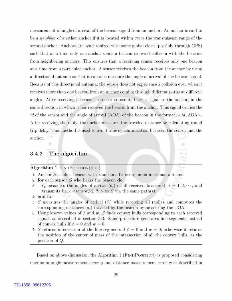
measurement of angle of arrival of the beacon signal from an anchor. An anchor is said to
be a neighbor of another anchor if it is located within twice the transmission range of the
second anchor. Anchors are synchronized with some global clock (possibly through GPS)
such that at a time only one anchor sends a beacon to avoid collision with the beacons
from neighboring anchors. This ensures that a receiving sensor receives only one beacon
at a time from a particular anchor. A sensor receives the beacon from the anchor by using
a directional antenna so that it can also measure the angle of arrival of the beacon signal.
Because of this directional antenna, the sensor does not experience a collision even when it
receives more than one beacon from an anchor coming through different paths at different
angles. After receiving a beacon, a sensor transmits back a signal to the anchor, in the
same direction in which it has received the beacon from the anchor. This signal carries the
id of the sensor and the angle of arrival (AOA) of the beacon in the format, <id, AOA>.
After receiving the reply, the anchor measures the traveled distance by calculating round
trip delay. This method is used to avoid time synchronization between the sensor and the
anchor.
3.4.2 The algorithm
Algorithm 1 FindPosition(φ, w)
1: Anchor S sends a beacon with <anchor id> using omnidirectional antenna.2: for each sensor Q who hears the beacon do3: Q measures the angles of arrival (θi) of all received beacon(s), i = 1, 2, · · · , and
transmits back <sensor id, θi > to S via the same path(s).4: end for5: S measures the angles of arrival (δi) while receiving all replies and computes the
corresponding distances (di) traveled by the beacon by measuring the TOA.6: Using known values of φ and w, S finds convex hulls corresponding to each received
signals as described in section 3.3. Same procedure generates line segments insteadof convex hulls if φ = 0 and w = 0.
7: S returns intersection of the line segments if φ = 0 and w = 0; otherwise it returnsthe position of the center of mass of the intersection of all the convex hulls, as theposition of Q.
Based on above discussion, the Algorithm 1 (FindPosition) is proposed considering
maximum angle measurement error φ and distance measurement error w as described in
29
TH-1358_09612305
section 3.3. It finds the position of a sensor Q using the received beacon signals from an
anchor S. Algorithm returns approximate position as the center of mass of the intersection
of the generated convex hulls as in Theorem 3.3.1. In presence of measurement errors,
parallel reflectors do not have any impact on the localization method opposed to the
Lemma 3.2.5 proved in case of errorless range estimations. But if there is no measurement
errors in the environment, i.e. φ = 0 and w = 0, then a line segment is generated instead
of a convex hull corresponding to each signal. In this case accurate position is calculated
as the intersection of two FDLs according to the Theorem 3.2.6.
3.5 Simulation
In the simulation of our proposed Algorithm 1: FindPosition, we consider presence
of errors in both angle and distance measurements. Simulation is done on a MATLAB
platform considering random errors in TOA and AOA measurements within some given
maximum values. Sensors and anchors are placed randomly in a 10 meter by 10 meter
square area on a two dimensional plane. Communication range of the anchors are 25
meter. One-bound signals are generated randomly such that the traveled distance of any
signal obeys the communication range of the anchors. Since we generate one-bound signals
by choosing reflectors randomly, LOS paths may also be encountered, i.e., the signal paths
can be be one-bound as well as LOS. According to SpiderBat [56] and Cricket compass
[63], we consider that the measured angles are within ±5 degree of the actual angle, i.e.,
the value of φ is taken as 5 degree, which is the maximum measurement error in AOA
technique. In [56], authors showed that using ultrasonic signal, distance measurement can
be performed within an error of few millimeter when the range is around 15 meter. With
reference to both [56] and [72], where round trip delay is used, we consider a maximum
error of 0.02 meter in distance measurement for a communication range of 25 meter.
Though known values of maximum possible measurement errors are used for simulation,
yet for some unknown environment, it is possible to estimate the maximum possible
errors. It can be done either theoretically using environmental parameters or practically
by experiments.
In Table 3.1, we show sample outputs of ten different runs out of large number of
30
TH-1358_09612305
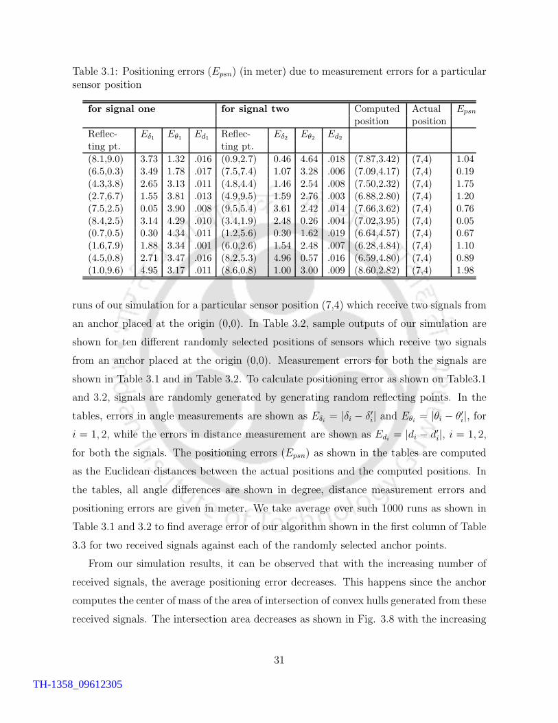
Table 3.1: Positioning errors (Epsn) (in meter) due to measurement errors for a particularsensor position
for signal one for signal two Computed Actual Epsn
position position
Reflec- Eδ1 Eθ1 Ed1 Reflec- Eδ2 Eθ2 Ed2
ting pt. ting pt.
(8.1,9.0) 3.73 1.32 .016 (0.9,2.7) 0.46 4.64 .018 (7.87,3.42) (7,4) 1.04(6.5,0.3) 3.49 1.78 .017 (7.5,7.4) 1.07 3.28 .006 (7.09,4.17) (7,4) 0.19(4.3,3.8) 2.65 3.13 .011 (4.8,4.4) 1.46 2.54 .008 (7.50,2.32) (7,4) 1.75(2.7,6.7) 1.55 3.81 .013 (4.9,9.5) 1.59 2.76 .003 (6.88,2.80) (7,4) 1.20(7.5,2.5) 0.05 3.90 .008 (9.5,5.4) 3.61 2.42 .014 (7.66,3.62) (7,4) 0.76(8.4,2.5) 3.14 4.29 .010 (3.4,1.9) 2.48 0.26 .004 (7.02,3.95) (7,4) 0.05(0.7,0.5) 0.30 4.34 .011 (1.2,5.6) 0.30 1.62 .019 (6.64,4.57) (7,4) 0.67(1.6,7.9) 1.88 3.34 .001 (6.0,2.6) 1.54 2.48 .007 (6.28,4.84) (7,4) 1.10(4.5,0.8) 2.71 3.47 .016 (8.2,5.3) 4.96 0.57 .016 (6.59,4.80) (7,4) 0.89(1.0,9.6) 4.95 3.17 .011 (8.6,0.8) 1.00 3.00 .009 (8.60,2.82) (7,4) 1.98
runs of our simulation for a particular sensor position (7,4) which receive two signals from
an anchor placed at the origin (0,0). In Table 3.2, sample outputs of our simulation are
shown for ten different randomly selected positions of sensors which receive two signals
from an anchor placed at the origin (0,0). Measurement errors for both the signals are
shown in Table 3.1 and in Table 3.2. To calculate positioning error as shown on Table3.1
and 3.2, signals are randomly generated by generating random reflecting points. In the
tables, errors in angle measurements are shown as Eδi = |δi − δ′i| and Eθi = |θi − θ′i|, fori = 1, 2, while the errors in distance measurement are shown as Edi = |di − d′i|, i = 1, 2,
for both the signals. The positioning errors (Epsn) as shown in the tables are computed
as the Euclidean distances between the actual positions and the computed positions. In
the tables, all angle differences are shown in degree, distance measurement errors and
positioning errors are given in meter. We take average over such 1000 runs as shown in
Table 3.1 and 3.2 to find average error of our algorithm shown in the first column of Table
3.3 for two received signals against each of the randomly selected anchor points.
From our simulation results, it can be observed that with the increasing number of
received signals, the average positioning error decreases. This happens since the anchor
computes the center of mass of the area of intersection of convex hulls generated from these
received signals. The intersection area decreases as shown in Fig. 3.8 with the increasing
31
TH-1358_09612305
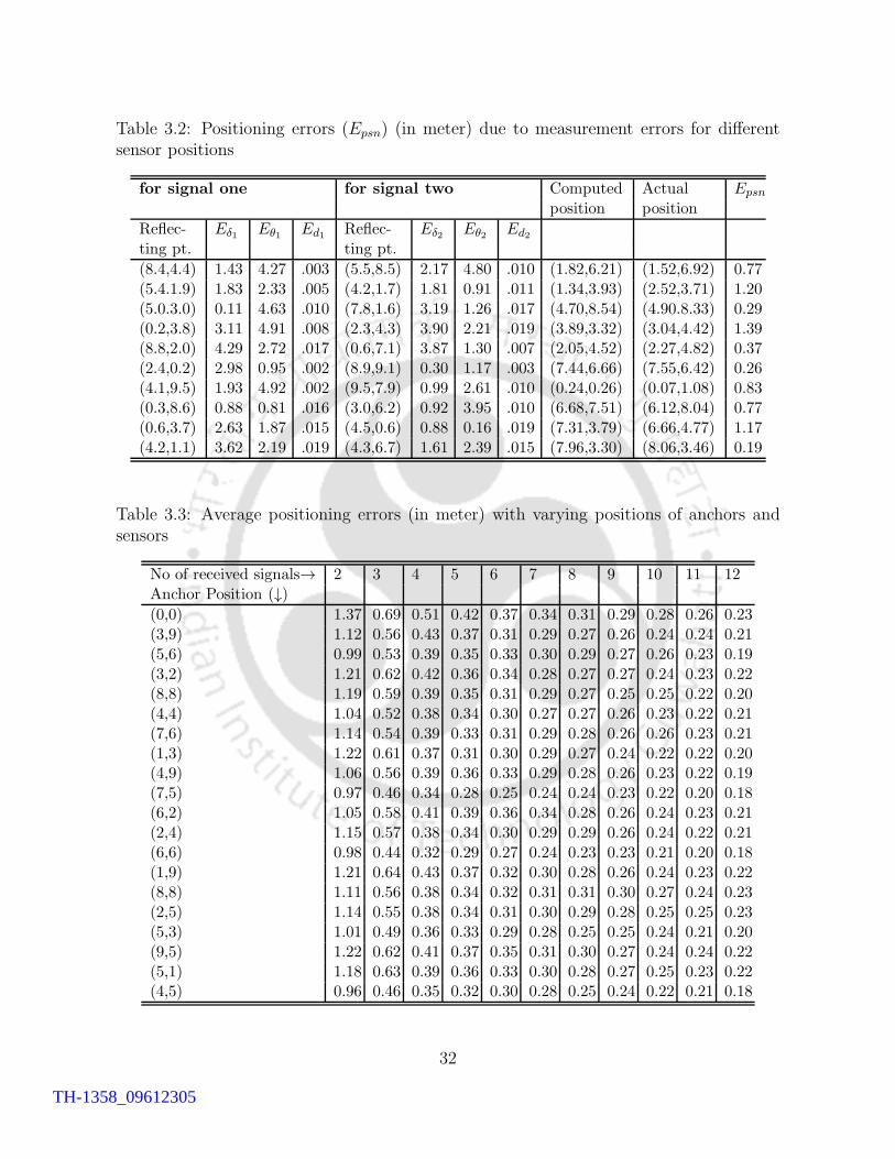
Table 3.2: Positioning errors (Epsn) (in meter) due to measurement errors for differentsensor positions
for signal one for signal two Computed Actual Epsn
position position
Reflec- Eδ1 Eθ1 Ed1 Reflec- Eδ2 Eθ2 Ed2
ting pt. ting pt.
(8.4,4.4) 1.43 4.27 .003 (5.5,8.5) 2.17 4.80 .010 (1.82,6.21) (1.52,6.92) 0.77(5.4.1.9) 1.83 2.33 .005 (4.2,1.7) 1.81 0.91 .011 (1.34,3.93) (2.52,3.71) 1.20(5.0.3.0) 0.11 4.63 .010 (7.8,1.6) 3.19 1.26 .017 (4.70,8.54) (4.90.8.33) 0.29(0.2,3.8) 3.11 4.91 .008 (2.3,4.3) 3.90 2.21 .019 (3.89,3.32) (3.04,4.42) 1.39(8.8,2.0) 4.29 2.72 .017 (0.6,7.1) 3.87 1.30 .007 (2.05,4.52) (2.27,4.82) 0.37(2.4,0.2) 2.98 0.95 .002 (8.9,9.1) 0.30 1.17 .003 (7.44,6.66) (7.55,6.42) 0.26(4.1,9.5) 1.93 4.92 .002 (9.5,7.9) 0.99 2.61 .010 (0.24,0.26) (0.07,1.08) 0.83(0.3,8.6) 0.88 0.81 .016 (3.0,6.2) 0.92 3.95 .010 (6.68,7.51) (6.12,8.04) 0.77(0.6,3.7) 2.63 1.87 .015 (4.5,0.6) 0.88 0.16 .019 (7.31,3.79) (6.66,4.77) 1.17(4.2,1.1) 3.62 2.19 .019 (4.3,6.7) 1.61 2.39 .015 (7.96,3.30) (8.06,3.46) 0.19
Table 3.3: Average positioning errors (in meter) with varying positions of anchors andsensors
No of received signals→ 2 3 4 5 6 7 8 9 10 11 12Anchor Position (↓)(0,0) 1.37 0.69 0.51 0.42 0.37 0.34 0.31 0.29 0.28 0.26 0.23(3,9) 1.12 0.56 0.43 0.37 0.31 0.29 0.27 0.26 0.24 0.24 0.21(5,6) 0.99 0.53 0.39 0.35 0.33 0.30 0.29 0.27 0.26 0.23 0.19(3,2) 1.21 0.62 0.42 0.36 0.34 0.28 0.27 0.27 0.24 0.23 0.22(8,8) 1.19 0.59 0.39 0.35 0.31 0.29 0.27 0.25 0.25 0.22 0.20(4,4) 1.04 0.52 0.38 0.34 0.30 0.27 0.27 0.26 0.23 0.22 0.21(7,6) 1.14 0.54 0.39 0.33 0.31 0.29 0.28 0.26 0.26 0.23 0.21(1,3) 1.22 0.61 0.37 0.31 0.30 0.29 0.27 0.24 0.22 0.22 0.20(4,9) 1.06 0.56 0.39 0.36 0.33 0.29 0.28 0.26 0.23 0.22 0.19(7,5) 0.97 0.46 0.34 0.28 0.25 0.24 0.24 0.23 0.22 0.20 0.18(6,2) 1.05 0.58 0.41 0.39 0.36 0.34 0.28 0.26 0.24 0.23 0.21(2,4) 1.15 0.57 0.38 0.34 0.30 0.29 0.29 0.26 0.24 0.22 0.21(6,6) 0.98 0.44 0.32 0.29 0.27 0.24 0.23 0.23 0.21 0.20 0.18(1,9) 1.21 0.64 0.43 0.37 0.32 0.30 0.28 0.26 0.24 0.23 0.22(8,8) 1.11 0.56 0.38 0.34 0.32 0.31 0.31 0.30 0.27 0.24 0.23(2,5) 1.14 0.55 0.38 0.34 0.31 0.30 0.29 0.28 0.25 0.25 0.23(5,3) 1.01 0.49 0.36 0.33 0.29 0.28 0.25 0.25 0.24 0.21 0.20(9,5) 1.22 0.62 0.41 0.37 0.35 0.31 0.30 0.27 0.24 0.24 0.22(5,1) 1.18 0.63 0.39 0.36 0.33 0.30 0.28 0.27 0.25 0.23 0.22(4,5) 0.96 0.46 0.35 0.32 0.30 0.28 0.25 0.24 0.22 0.21 0.18
32
TH-1358_09612305
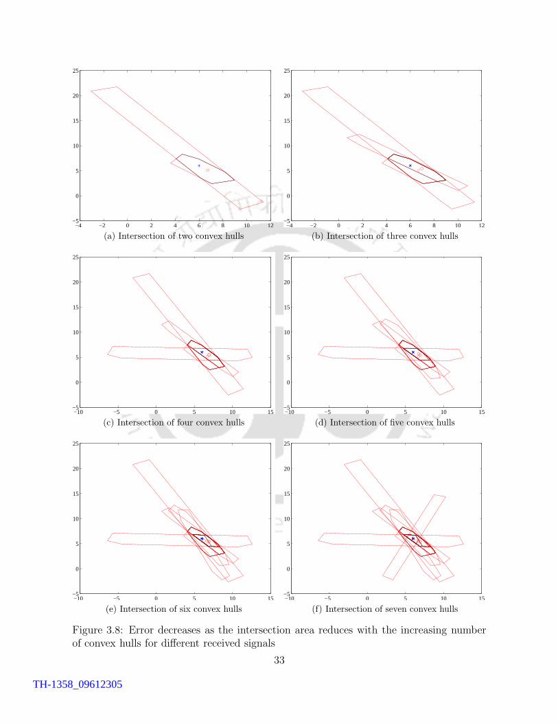
−4 −2 0 2 4 6 8 10 12−5
0
5
10
15
20
25
(a) Intersection of two convex hulls−4 −2 0 2 4 6 8 10 12
−5
0
5
10
15
20
25
(b) Intersection of three convex hulls
−10 −5 0 5 10 15−5
0
5
10
15
20
25
(c) Intersection of four convex hulls−10 −5 0 5 10 15−5
0
5
10
15
20
25
(d) Intersection of five convex hulls
−10 −5 0 5 10 15−5
0
5
10
15
20
25
(e) Intersection of six convex hulls−10 −5 0 5 10 15−5
0
5
10
15
20
25
(f) Intersection of seven convex hulls
Figure 3.8: Error decreases as the intersection area reduces with the increasing numberof convex hulls for different received signals
33
TH-1358_09612305
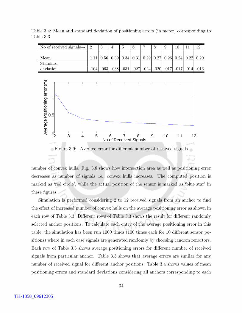
Table 3.4: Mean and standard deviation of positioning errors (in meter) corresponding toTable 3.3
No of received signals→ 2 3 4 5 6 7 8 9 10 11 12
Mean 1.11 0.56 0.39 0.34 0.31 0.29 0.27 0.26 0.24 0.22 0.20
Standarddeviation .104 .063 .038 .031 .027 .024 .020 .017 .017 .014 .016
2 3 4 5 6 7 8 9 10 11 120
0.5
1
No of Received Signals
Ave
rage
Pos
ition
ing
erro
r (m
)
Figure 3.9: Average error for different number of received signals
number of convex hulls. Fig. 3.8 shows how intersection area as well as positioning error
decreases as number of signals i.e., convex hulls increases. The computed position is
marked as ‘red circle’, while the actual position of the sensor is marked as ‘blue star’ in
these figures.
Simulation is performed considering 2 to 12 received signals from an anchor to find
the effect of increased number of convex hulls on the average positioning error as shown in
each row of Table 3.3. Different rows of Table 3.3 shows the result for different randomly
selected anchor positions. To calculate each entry of the average positioning error in this
table, the simulation has been run 1000 times (100 times each for 10 different sensor po-
sitions) where in each case signals are generated randomly by choosing random reflectors.
Each row of Table 3.3 shows average positioning errors for different number of received
signals from particular anchor. Table 3.3 shows that average errors are similar for any
number of received signal for different anchor positions. Table 3.4 shows values of mean
positioning errors and standard deviations considering all anchors corresponding to each
34
TH-1358_09612305
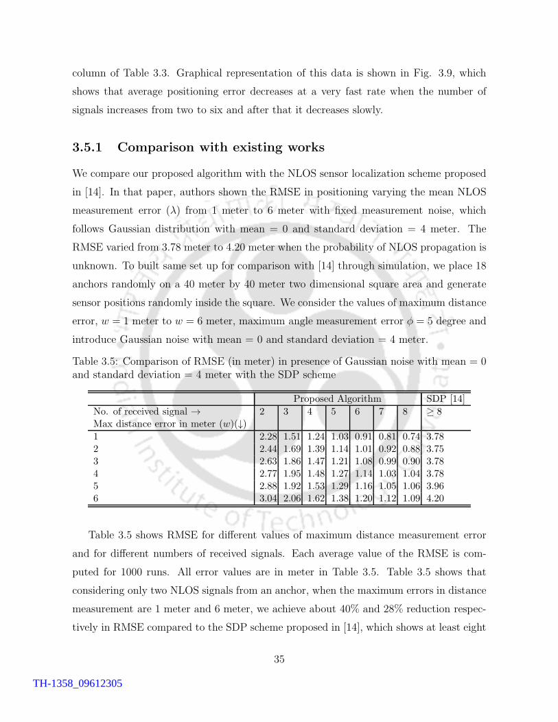
column of Table 3.3. Graphical representation of this data is shown in Fig. 3.9, which
shows that average positioning error decreases at a very fast rate when the number of
signals increases from two to six and after that it decreases slowly.
3.5.1 Comparison with existing works
We compare our proposed algorithm with the NLOS sensor localization scheme proposed
in [14]. In that paper, authors shown the RMSE in positioning varying the mean NLOS
measurement error (λ) from 1 meter to 6 meter with fixed measurement noise, which
follows Gaussian distribution with mean = 0 and standard deviation = 4 meter. The
RMSE varied from 3.78 meter to 4.20 meter when the probability of NLOS propagation is
unknown. To built same set up for comparison with [14] through simulation, we place 18
anchors randomly on a 40 meter by 40 meter two dimensional square area and generate
sensor positions randomly inside the square. We consider the values of maximum distance
error, w = 1 meter to w = 6 meter, maximum angle measurement error φ = 5 degree and
introduce Gaussian noise with mean = 0 and standard deviation = 4 meter.
Table 3.5: Comparison of RMSE (in meter) in presence of Gaussian noise with mean = 0and standard deviation = 4 meter with the SDP scheme
Proposed Algorithm SDP [14]
No. of received signal → 2 3 4 5 6 7 8 ≥ 8Max distance error in meter (w)(↓)1 2.28 1.51 1.24 1.03 0.91 0.81 0.74 3.782 2.44 1.69 1.39 1.14 1.01 0.92 0.88 3.753 2.63 1.86 1.47 1.21 1.08 0.99 0.90 3.784 2.77 1.95 1.48 1.27 1.14 1.03 1.04 3.785 2.88 1.92 1.53 1.29 1.16 1.05 1.06 3.966 3.04 2.06 1.62 1.38 1.20 1.12 1.09 4.20
Table 3.5 shows RMSE for different values of maximum distance measurement error
and for different numbers of received signals. Each average value of the RMSE is com-
puted for 1000 runs. All error values are in meter in Table 3.5. Table 3.5 shows that
considering only two NLOS signals from an anchor, when the maximum errors in distance
measurement are 1 meter and 6 meter, we achieve about 40% and 28% reduction respec-
tively in RMSE compared to the SDP scheme proposed in [14], which shows at least eight
35
TH-1358_09612305
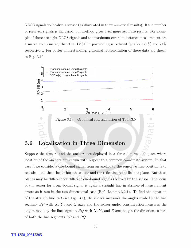
NLOS signals to localize a sensor (as illustrated in their numerical results). If the number
of received signals is increased, our method gives even more accurate results. For exam-
ple, if there are eight NLOS signals and the maximum errors in distance measurement are
1 meter and 6 meter, then the RMSE in positioning is reduced by about 81% and 74%
respectively. For better understanding, graphical representation of these data are shown
in Fig. 3.10.
1 2 3 4 5 660
1
2
3
4
5
6
Distace error (m)
RM
SE
(m
)
Proposed scheme using 8 signalsProposed scheme using 2 signalsSDP in [4] using at least 8 signals
Figure 3.10: Graphical representation of Table3.5
3.6 Localization in Three Dimension
Suppose the sensors and the anchors are deployed in a three dimensional space where
location of the anchors are known with respect to a common coordinate system. In that
case if we consider a one-bound signal from an anchor to the sensor, whose position is to
be calculated then the anchor, the sensor and the reflecting point lie on a plane. But these
planes may be different for different one-bound signals received by the sensor. The locus
of the sensor for a one-bound signal is again a straight line in absence of measurement
errors as it was in the two dimensional case (Ref. Lemma 3.2.1). To find the equation
of the straight line AB (see Fig. 3.1), the anchor measures the angles made by the line
segment SP with X , Y , and Z axes and the sensor under consideration measures the
angles made by the line segment PQ with X , Y , and Z axes to get the direction cosines
of both the line segments SP and PQ.
36
TH-1358_09612305
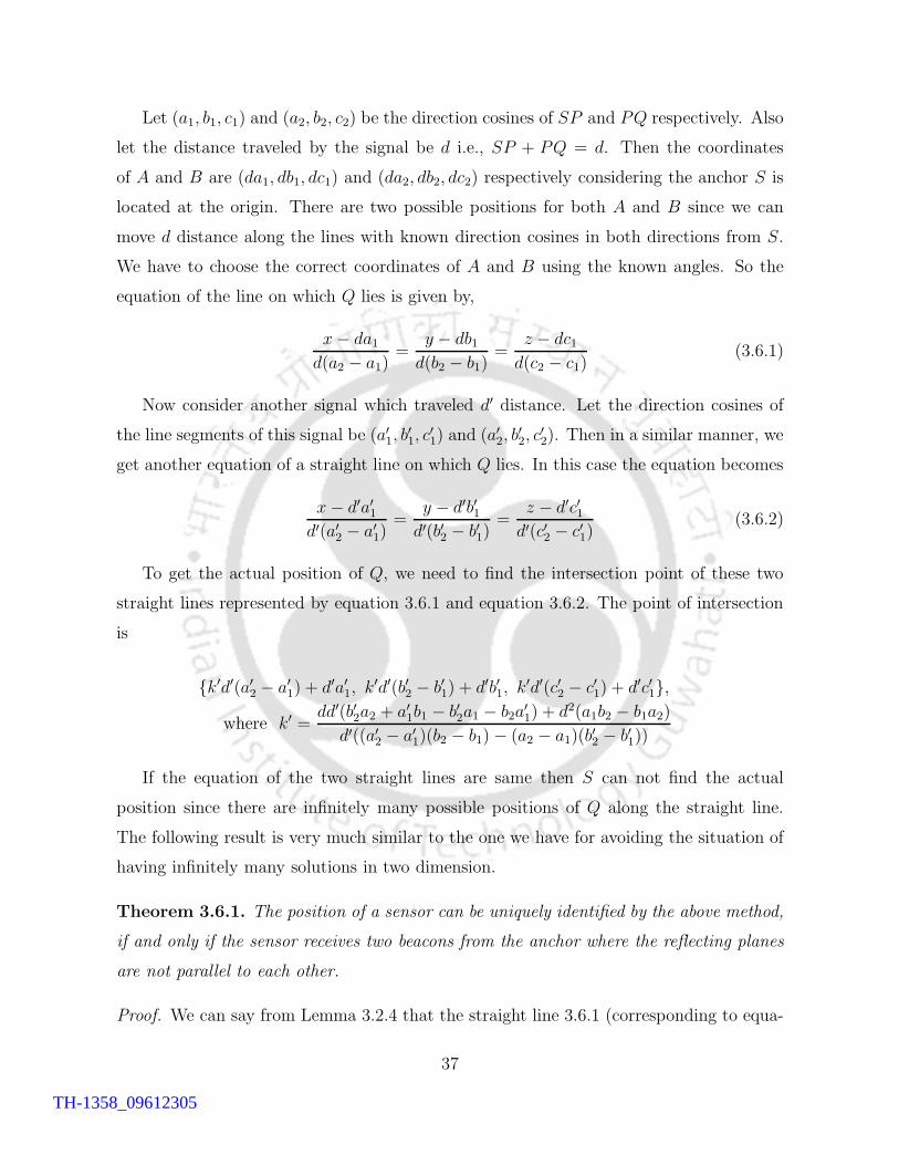
Let (a1, b1, c1) and (a2, b2, c2) be the direction cosines of SP and PQ respectively. Also
let the distance traveled by the signal be d i.e., SP + PQ = d. Then the coordinates
of A and B are (da1, db1, dc1) and (da2, db2, dc2) respectively considering the anchor S is
located at the origin. There are two possible positions for both A and B since we can
move d distance along the lines with known direction cosines in both directions from S.
We have to choose the correct coordinates of A and B using the known angles. So the
equation of the line on which Q lies is given by,
x− da1d(a2 − a1)
=y − db1
d(b2 − b1)=
z − dc1d(c2 − c1)
(3.6.1)
Now consider another signal which traveled d′ distance. Let the direction cosines of
the line segments of this signal be (a′1, b′1, c
′1) and (a′2, b
′2, c
′2). Then in a similar manner, we
get another equation of a straight line on which Q lies. In this case the equation becomes
x− d′a′1d′(a′2 − a′1)
=y − d′b′1
d′(b′2 − b′1)=
z − d′c′1d′(c′2 − c′1)
(3.6.2)
To get the actual position of Q, we need to find the intersection point of these two
straight lines represented by equation 3.6.1 and equation 3.6.2. The point of intersection
is
{k′d′(a′2 − a′1) + d′a′1, k′d′(b′2 − b′1) + d′b′1, k′d′(c′2 − c′1) + d′c′1},
where k′ =dd′(b′2a2 + a′1b1 − b′2a1 − b2a
′1) + d2(a1b2 − b1a2)
d′((a′2 − a′1)(b2 − b1)− (a2 − a1)(b′2 − b′1))
If the equation of the two straight lines are same then S can not find the actual
position since there are infinitely many possible positions of Q along the straight line.
The following result is very much similar to the one we have for avoiding the situation of
having infinitely many solutions in two dimension.
Theorem 3.6.1. The position of a sensor can be uniquely identified by the above method,
if and only if the sensor receives two beacons from the anchor where the reflecting planes
are not parallel to each other.
Proof. We can say from Lemma 3.2.4 that the straight line 3.6.1 (corresponding to equa-
37
TH-1358_09612305
tion 3.6.1) is parallel to the bisector of the angle ∠SPQ (see Fig. 3.1) which is perpendic-
ular to the reflecting plane. Similarly, the straight line 3.6.2 (corresponding to equation
3.6.2) is also perpendicular to the other reflecting plane from where the corresponding
signal is received.
First assume that the reflecting planes are not parallel. Then the straight lines 3.6.1
and 3.6.2 are also not parallel. So, these straight lines intersect at Q. Conversely, assume
that we can uniquely compute the position of Q. That means, the straight lines 3.6.1 and
3.6.2 intersect, i.e., the slopes of the straight lines 3.6.1 and 3.6.2 are different. Hence,
the planes which are perpendicular to the straight lines 3.6.1 and 3.6.2 are not parallel,
i.e., the reflecting surfaces are not parallel to each other.
3.7 Robust Localization in NLOS
In this section we show that our proposed localization technique is robust if wrong posi-
tion information get assigned to some sensors by accident. Consequently, anchor receives
wrong angle and distance information from those sensors. Here wrong position informa-
tion means wrong angle information somehow sent by the sensor to the anchor as well as
the unwilling occurrence of time delay at the sensor while replying the signal back. Dis-
tance measurement errors generate due to unwilling delay introduced by the sensor while
replying back the received signal as anchor uses round trip delay to calculate distance.
We show below that in absence of measurement errors, an anchor can detect such kind of
errors generated at the sensor.
Theorem 3.7.1. In absence of errors in measurement, three signals are sufficient for
the anchor to detect inconsistent angle of arrival and/or distance information sent by the
sensor.
Proof. Suppose a sensor Q receives three reflected signals from an anchor S via P ′, P ′′,
and P ′′′ as shown in Fig. 3.11. First consider the signals SQ via P ′ and SQ via P ′′. Let
S receives wrong information θ′1 and θ′2 instead of θ1 and θ2 and calculates wrong traveled
distance due to delay in reply at Q. S calculates two FDLs which intersect at Q′, say,
as shown in Fig. 3.11. S can misinterpret Q′ as the correct position of Q if it would
38
TH-1358_09612305
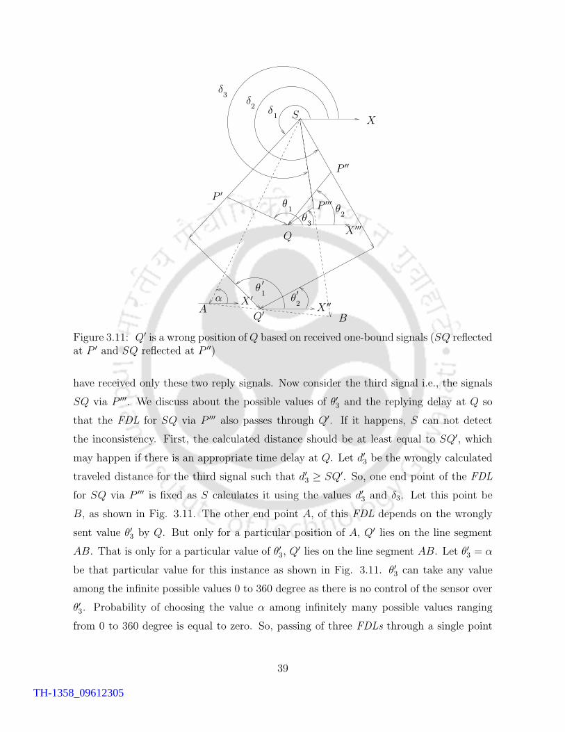
α
δδ
δ
θθθ
θθ′
′
1
1
1
2
2
2
3
3
S
AB
Q
Q′
P ′
P ′′
P ′′′
X
X ′X ′′
X ′′′
Figure 3.11: Q′ is a wrong position ofQ based on received one-bound signals (SQ reflectedat P ′ and SQ reflected at P ′′)
have received only these two reply signals. Now consider the third signal i.e., the signals
SQ via P ′′′. We discuss about the possible values of θ′3 and the replying delay at Q so
that the FDL for SQ via P ′′′ also passes through Q′. If it happens, S can not detect
the inconsistency. First, the calculated distance should be at least equal to SQ′, which
may happen if there is an appropriate time delay at Q. Let d′3 be the wrongly calculated
traveled distance for the third signal such that d′3 ≥ SQ′. So, one end point of the FDL
for SQ via P ′′′ is fixed as S calculates it using the values d′3 and δ3. Let this point be
B, as shown in Fig. 3.11. The other end point A, of this FDL depends on the wrongly
sent value θ′3 by Q. But only for a particular position of A, Q′ lies on the line segment
AB. That is only for a particular value of θ′3, Q′ lies on the line segment AB. Let θ′3 = α
be that particular value for this instance as shown in Fig. 3.11. θ′3 can take any value
among the infinite possible values 0 to 360 degree as there is no control of the sensor over
θ′3. Probability of choosing the value α among infinitely many possible values ranging
from 0 to 360 degree is equal to zero. So, passing of three FDLs through a single point
39
TH-1358_09612305
is an impossible event if arbitrarily wrong information are accumulated at S. Hence, in
absence of errors in measurement, three signals are sufficient for S to detect inconsistent
information.
3.8 Conclusions
In this work, we have proposed a deterministic algorithm to find the position of a sensor
based on receiving at least two reflected signals without having any knowledge about
the positions of those reflectors. If sensor receives signals from different anchors then
communication between the anchors are required. Simulation results in presence of mea-
surement errors show better positioning accuracy of proposed scheme compared to [14].
The positioning error does not increase significantly with significant increment of distance
measurement error. Strong point of our approach is that our algorithm works in a sparse
network since only two reflected signals from an anchor are sufficient for finding the posi-
tion of a sensor. We have also shown that with accurate range measurements the anchor
can detect some erroneous situations like wrong angle information and error in round trip
delay while localizing the sensor. However, further studies are needed for detecting such
situations in presence of errors in measurements.
40
TH-1358_09612305
Chapter 4
Analysis of Multiple-Bound Signals
towards Localization
4.1 Introduction
In this chapter we generalize the localization problem of the previous chapter by allowing
multiple reflections of a signal before reaching to a sensor. We first solve it for two-bound
signals and then generalize it for multiple-bound signals. An area of presence is found
for a sensor which receives a signal reflected more than once. Since it is not possible
to know number of reflections of a received signal, we propose solution for unknown-
bound signal. Theoretically, we prove that it is possible to localize sensor which receives
unknown-bound signals, within an area, assuming that we know the maximum possible
number of bounds in the environment. Comparison with trilateration shows improvement
when sensor receives three unknown-bound signals from different anchors.
4.1.1 Our contribution
In this chapter we analyze multiple-bound signals so that sensor can use received signals
irrespective of the number of reflections. If signal traverses d distance from an anchor
before reaching the sensor then the possible location of the sensor is always within a
circle of radius d centering at the anchor. Now using information of a received unknown-
bound signal, we are able compute a circle with radius less than d, where the sensor is
41
TH-1358_09612305
bound to reside. We also propose a technique to localize sensor when it receives multiple-
bound signals and the number of bounds are unknown. In this case, assumption is that
the maximum possible number of bounds in the system is known. To the best of our
knowledge there is no work in literature considering multiple-bound (reflected more than
once) signals to locate the position of a sensor deterministically. Simulation results show
that on an average 35% improvement in terms of area of presence and 40% improvement
in terms of average error over trilateration using three two-bound signals, whereas on an
average, 10% improvement in terms of area of presence and 4% improvement in terms of
average error over trilateration when a sensor receives three unknown-bound signals from
different anchors.
The organization of the remaining part of this chapter is as follows. Basic idea is
explained in section 4.2. Analysis of two-bound signal is given in section 4.3. Analysis
of multiple-bound signal is discussed in section 4.4. In section 4.5, area of presence of
a sensor which received an unknown-bound signal is computed. Proposed localization
algorithm is presented in section 4.6. Comparison with simulation results are shown in
section 4.7. Finally, we conclude in section 4.8.
4.2 Basic Idea
According to the algorithm proposed in the previous chapter, position of a sensor is
calculated based on TOA and AOA measurement techniques under the model which
allows up to one-bound signals. Using AOA technique, receiving angles of arrival θ at the
sensor and δ at the anchor are measured, whereas the path length d traveled by the signal
is measured by TOA technique. Following theorem shows that in presence of multiple-
bound (more than one-bound) signal, AOA and TOA measurements are not sufficient to
localize a sensor.
Theorem 4.2.1. (Impossibility) Under the model which allows multiple-bound signal,
TOA and AOA measurements are insufficient to locate a sensor in a specific position with
multiple-bound signals.
Proof. We prove it for a two-bound signal. Let a sensor Q receives two-bound signal from
42
TH-1358_09612305
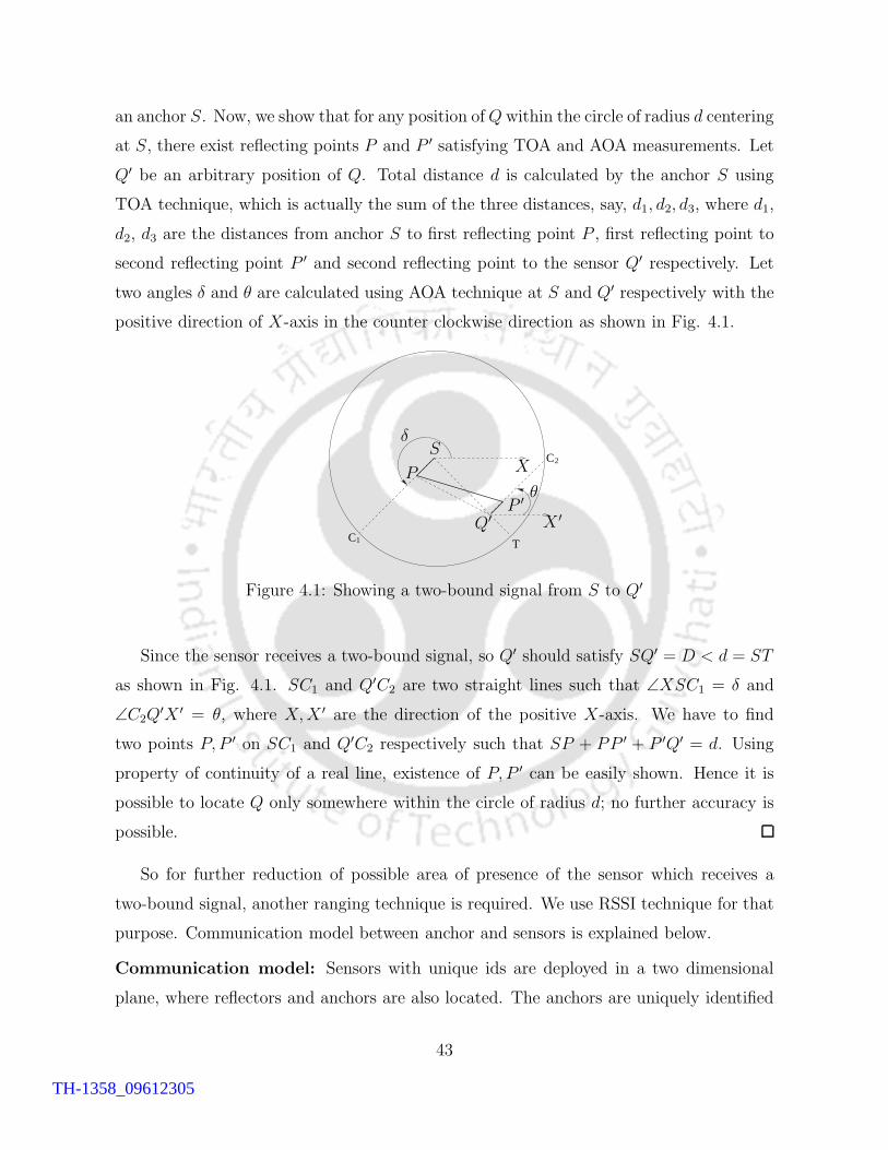
an anchor S. Now, we show that for any position ofQ within the circle of radius d centering
at S, there exist reflecting points P and P ′ satisfying TOA and AOA measurements. Let
Q′ be an arbitrary position of Q. Total distance d is calculated by the anchor S using
TOA technique, which is actually the sum of the three distances, say, d1, d2, d3, where d1,
d2, d3 are the distances from anchor S to first reflecting point P , first reflecting point to
second reflecting point P ′ and second reflecting point to the sensor Q′ respectively. Let
two angles δ and θ are calculated using AOA technique at S and Q′ respectively with the
positive direction of X-axis in the counter clockwise direction as shown in Fig. 4.1.
C
1
2
T
C
θ
δ
Q′
S
P
P ′
X
X ′
Figure 4.1: Showing a two-bound signal from S to Q′
Since the sensor receives a two-bound signal, so Q′ should satisfy SQ′ = D < d = ST
as shown in Fig. 4.1. SC1 and Q′C2 are two straight lines such that ∠XSC1 = δ and
∠C2Q′X ′ = θ, where X,X ′ are the direction of the positive X-axis. We have to find
two points P, P ′ on SC1 and Q′C2 respectively such that SP + PP ′ + P ′Q′ = d. Using
property of continuity of a real line, existence of P, P ′ can be easily shown. Hence it is
possible to locate Q only somewhere within the circle of radius d; no further accuracy is
possible.
So for further reduction of possible area of presence of the sensor which receives a
two-bound signal, another ranging technique is required. We use RSSI technique for that
purpose. Communication model between anchor and sensors is explained below.
Communication model: Sensors with unique ids are deployed in a two dimensional
plane, where reflectors and anchors are also located. The anchors are uniquely identified
43
TH-1358_09612305
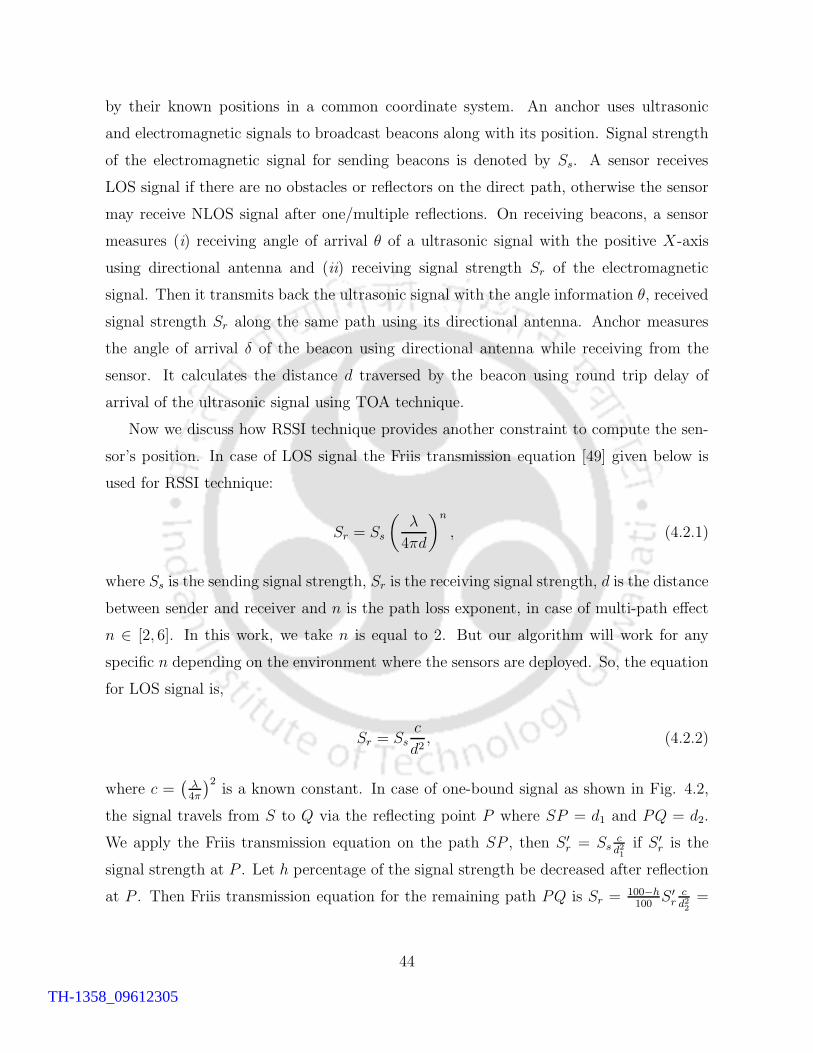
by their known positions in a common coordinate system. An anchor uses ultrasonic
and electromagnetic signals to broadcast beacons along with its position. Signal strength
of the electromagnetic signal for sending beacons is denoted by Ss. A sensor receives
LOS signal if there are no obstacles or reflectors on the direct path, otherwise the sensor
may receive NLOS signal after one/multiple reflections. On receiving beacons, a sensor
measures (i) receiving angle of arrival θ of a ultrasonic signal with the positive X-axis
using directional antenna and (ii) receiving signal strength Sr of the electromagnetic
signal. Then it transmits back the ultrasonic signal with the angle information θ, received
signal strength Sr along the same path using its directional antenna. Anchor measures
the angle of arrival δ of the beacon using directional antenna while receiving from the
sensor. It calculates the distance d traversed by the beacon using round trip delay of
arrival of the ultrasonic signal using TOA technique.
Now we discuss how RSSI technique provides another constraint to compute the sen-
sor’s position. In case of LOS signal the Friis transmission equation [49] given below is
used for RSSI technique:
Sr = Ss
(
λ
4πd
)n
, (4.2.1)
where Ss is the sending signal strength, Sr is the receiving signal strength, d is the distance
between sender and receiver and n is the path loss exponent, in case of multi-path effect
n ∈ [2, 6]. In this work, we take n is equal to 2. But our algorithm will work for any
specific n depending on the environment where the sensors are deployed. So, the equation
for LOS signal is,
Sr = Ssc
d2, (4.2.2)
where c =(
λ4π
)2is a known constant. In case of one-bound signal as shown in Fig. 4.2,
the signal travels from S to Q via the reflecting point P where SP = d1 and PQ = d2.
We apply the Friis transmission equation on the path SP , then S ′r = Ss
cd21
if S ′r is the
signal strength at P . Let h percentage of the signal strength be decreased after reflection
at P . Then Friis transmission equation for the remaining path PQ is Sr =100−h100
S ′r
cd22
=
44
TH-1358_09612305
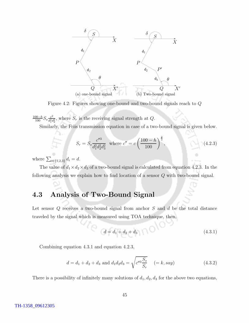
d
2
1
d
θ
δ
Q
S
P
X
X ′
(a) one-bound signal
d1
d
d
2
3 θ
δ
Q
S
P
P ′
X
X ′
(b) Two-bound signal
Figure 4.2: Figures showing one-bound and two-bound signals reach to Q
100−h100
Ssc2
d21d22
, where Sr is the receiving signal strength at Q.
Similarly, the Friis transmission equation in case of a two-bound signal is given below.
Sr = Ssc′′3
d21d22d
23
where c′′ = c
(
100− h
100
)2
3
, (4.2.3)
where∑
i∈{1,2,3} di = d.
The value of d1×d2×d3 of a two-bound signal is calculated from equation 4.2.3. In the
following analysis we explain how to find location of a sensor Q with two-bound signal.
4.3 Analysis of Two-Bound Signal
Let sensor Q receives a two-bound signal from anchor S and d be the total distance
traveled by the signal which is measured using TOA technique, then,
d = d1 + d2 + d3 (4.3.1)
Combining equation 4.3.1 and equation 4.2.3,
d = d1 + d2 + d3 and d1d2d3 =
√
c′′3Ss
Sr(= k, say) (4.3.2)
There is a possibility of infinitely many solutions of d1, d2, d3 for the above two equations,
45
TH-1358_09612305
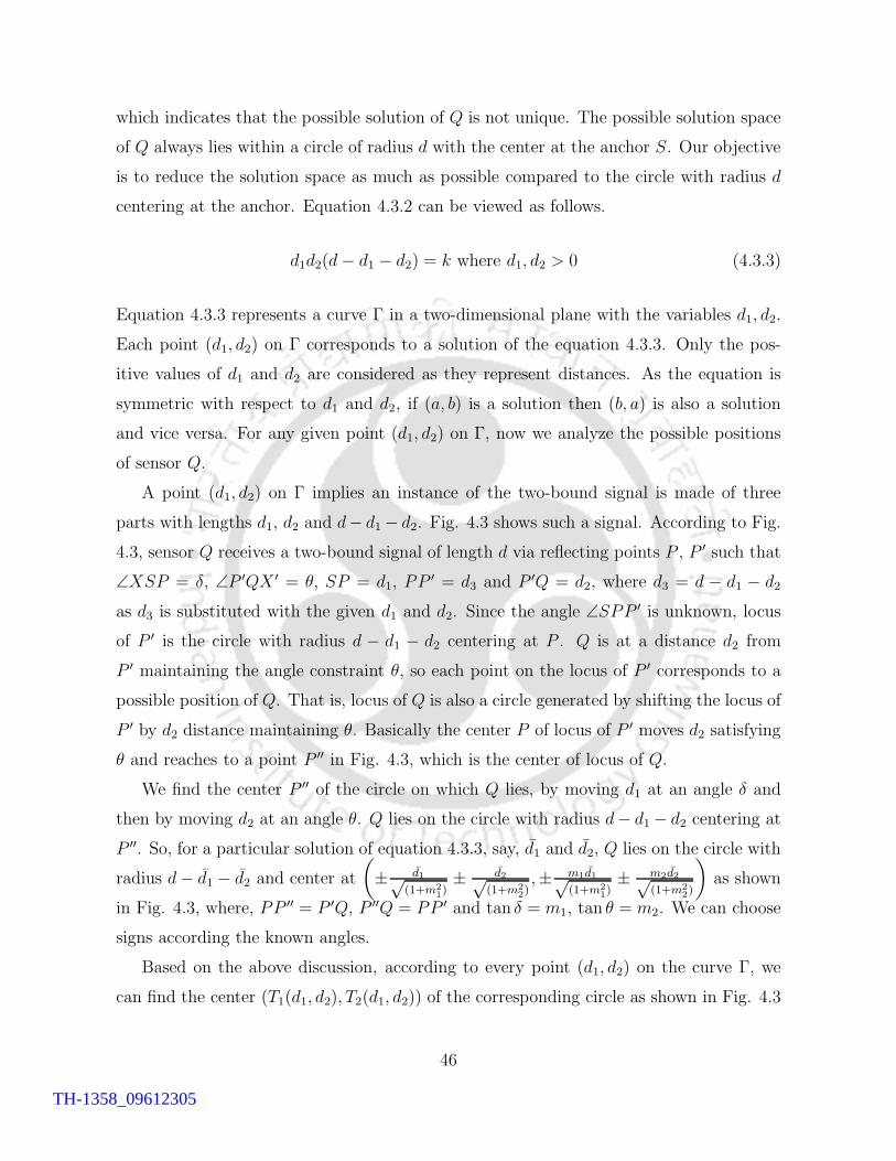
which indicates that the possible solution of Q is not unique. The possible solution space
of Q always lies within a circle of radius d with the center at the anchor S. Our objective
is to reduce the solution space as much as possible compared to the circle with radius d
centering at the anchor. Equation 4.3.2 can be viewed as follows.
d1d2(d− d1 − d2) = k where d1, d2 > 0 (4.3.3)
Equation 4.3.3 represents a curve Γ in a two-dimensional plane with the variables d1, d2.
Each point (d1, d2) on Γ corresponds to a solution of the equation 4.3.3. Only the pos-
itive values of d1 and d2 are considered as they represent distances. As the equation is
symmetric with respect to d1 and d2, if (a, b) is a solution then (b, a) is also a solution
and vice versa. For any given point (d1, d2) on Γ, now we analyze the possible positions
of sensor Q.
A point (d1, d2) on Γ implies an instance of the two-bound signal is made of three
parts with lengths d1, d2 and d− d1 − d2. Fig. 4.3 shows such a signal. According to Fig.
4.3, sensor Q receives a two-bound signal of length d via reflecting points P , P ′ such that
∠XSP = δ, ∠P ′QX ′ = θ, SP = d1, PP ′ = d3 and P ′Q = d2, where d3 = d − d1 − d2
as d3 is substituted with the given d1 and d2. Since the angle ∠SPP ′ is unknown, locus
of P ′ is the circle with radius d − d1 − d2 centering at P . Q is at a distance d2 from
P ′ maintaining the angle constraint θ, so each point on the locus of P ′ corresponds to a
possible position of Q. That is, locus of Q is also a circle generated by shifting the locus of
P ′ by d2 distance maintaining θ. Basically the center P of locus of P ′ moves d2 satisfying
θ and reaches to a point P ′′ in Fig. 4.3, which is the center of locus of Q.
We find the center P ′′ of the circle on which Q lies, by moving d1 at an angle δ and
then by moving d2 at an angle θ. Q lies on the circle with radius d− d1 − d2 centering at
P ′′. So, for a particular solution of equation 4.3.3, say, d1 and d2, Q lies on the circle with
radius d− d1 − d2 and center at
(
± d1√(1+m2
1)± d2√
(1+m22),± m1d1√
(1+m21)± m2d2√
(1+m22)
)
as shown
in Fig. 4.3, where, PP ′′ = P ′Q, P ′′Q = PP ′ and tan δ = m1, tan θ = m2. We can choose
signs according the known angles.
Based on the above discussion, according to every point (d1, d2) on the curve Γ, we
can find the center (T1(d1, d2), T2(d1, d2)) of the corresponding circle as shown in Fig. 4.3
46
TH-1358_09612305
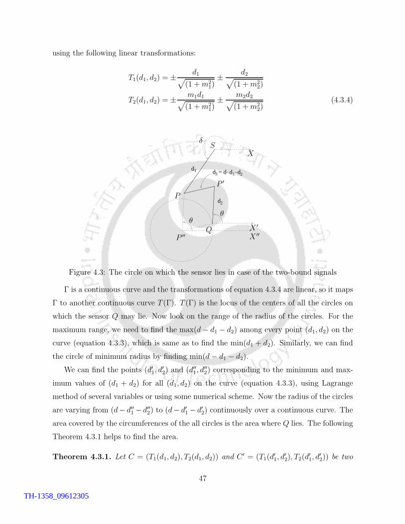
using the following linear transformations:
T1(d1, d2) = ± d1√
(1 +m21)
± d2√
(1 +m22)
T2(d1, d2) = ± m1d1√
(1 +m21)
± m2d2√
(1 +m22)
(4.3.4)
d = d 1
d 2
d 2 d1
3 d
θθ
δ
Q
S
P
P ′
X
X ′
P ′′ X ′′
Figure 4.3: The circle on which the sensor lies in case of the two-bound signals
Γ is a continuous curve and the transformations of equation 4.3.4 are linear, so it maps
Γ to another continuous curve T (Γ). T (Γ) is the locus of the centers of all the circles on
which the sensor Q may lie. Now look on the range of the radius of the circles. For the
maximum range, we need to find the max(d− d1 − d2) among every point (d1, d2) on the
curve (equation 4.3.3), which is same as to find the min(d1 + d2). Similarly, we can find
the circle of minimum radius by finding min(d− d1 − d2).
We can find the points (d′1, d′2) and (d′′1, d
′′2) corresponding to the minimum and max-
imum values of (d1 + d2) for all (d1, d2) on the curve (equation 4.3.3), using Lagrange
method of several variables or using some numerical scheme. Now the radius of the circles
are varying from (d− d′′1 − d′′2) to (d− d′1 − d′2) continuously over a continuous curve. The
area covered by the circumferences of the all circles is the area where Q lies. The following
Theorem 4.3.1 helps to find the area.
Theorem 4.3.1. Let C = (T1(d1, d2), T2(d1, d2)) and C ′ = (T1(d′1, d
′2), T2(d
′1, d
′2)) be two
47
TH-1358_09612305
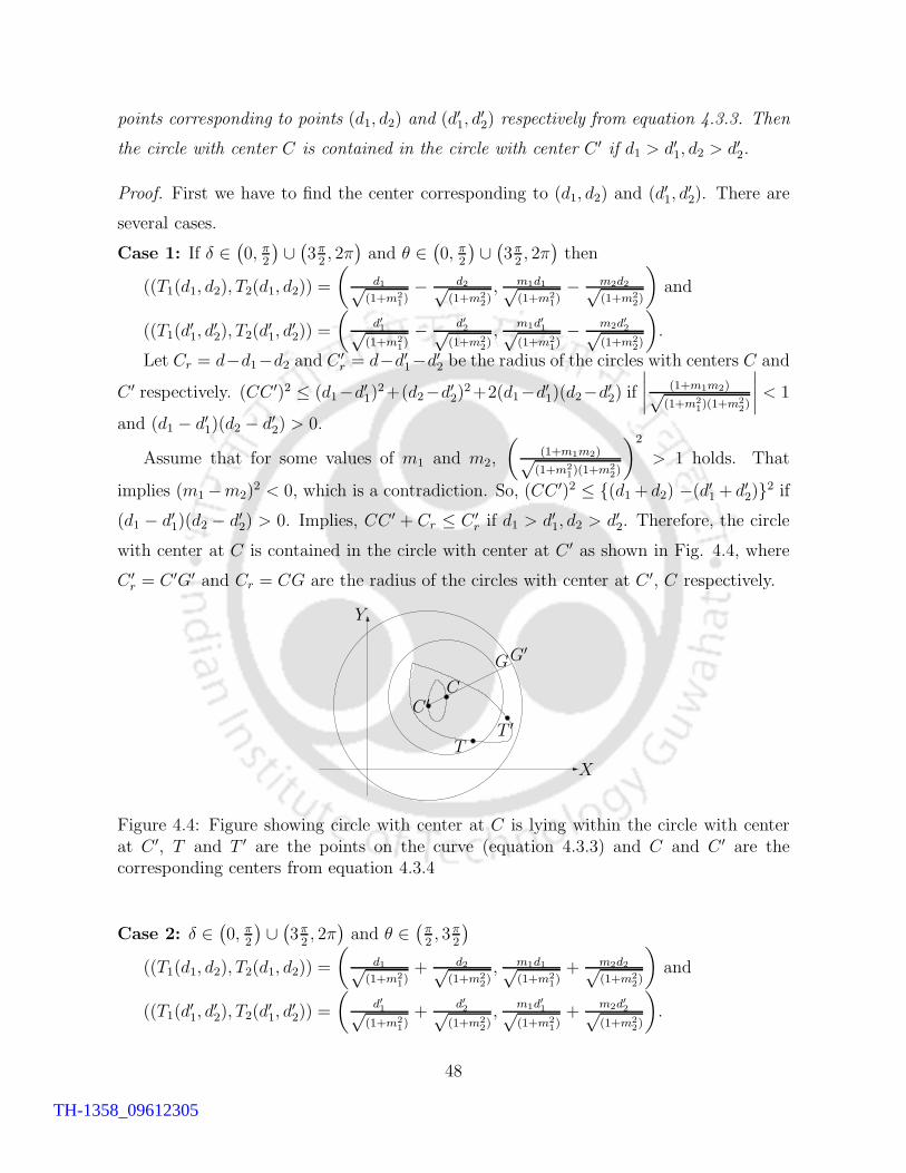
points corresponding to points (d1, d2) and (d′1, d′2) respectively from equation 4.3.3. Then
the circle with center C is contained in the circle with center C ′ if d1 > d′1, d2 > d′2.
Proof. First we have to find the center corresponding to (d1, d2) and (d′1, d′2). There are
several cases.
Case 1: If δ ∈(
0, π2
)
∪(
3π2, 2π
)
and θ ∈(
0, π2
)
∪(
3π2, 2π
)
then
((T1(d1, d2), T2(d1, d2)) =
(
d1√(1+m2
1)− d2√
(1+m22), m1d1√
(1+m21)− m2d2√
(1+m22)
)
and
((T1(d′1, d
′2), T2(d
′1, d
′2)) =
(
d′1√
(1+m21)− d′
2√(1+m2
2),
m1d′1√(1+m2
1)− m2d′2√
(1+m22)
)
.
Let Cr = d−d1−d2 and C ′r = d−d′1−d′2 be the radius of the circles with centers C and
C ′ respectively. (CC ′)2 ≤ (d1−d′1)2+(d2−d′2)
2+2(d1−d′1)(d2−d′2) if
∣
∣
∣
∣
(1+m1m2)√(1+m2
1)(1+m2
2)
∣
∣
∣
∣
< 1
and (d1 − d′1)(d2 − d′2) > 0.
Assume that for some values of m1 and m2,
(
(1+m1m2)√(1+m2
1)(1+m2
2)
)2
> 1 holds. That
implies (m1 −m2)2 < 0, which is a contradiction. So, (CC ′)2 ≤ {(d1 + d2) −(d′1 + d′2)}2 if
(d1 − d′1)(d2 − d′2) > 0. Implies, CC ′ + Cr ≤ C ′r if d1 > d′1, d2 > d′2. Therefore, the circle
with center at C is contained in the circle with center at C ′ as shown in Fig. 4.4, where
C ′r = C ′G′ and Cr = CG are the radius of the circles with center at C ′, C respectively.
TT ′
G′
C ′C
G
X
Y
Figure 4.4: Figure showing circle with center at C is lying within the circle with centerat C ′, T and T ′ are the points on the curve (equation 4.3.3) and C and C ′ are thecorresponding centers from equation 4.3.4
Case 2: δ ∈(
0, π2
)
∪(
3π2, 2π
)
and θ ∈(
π2, 3π
2
)
((T1(d1, d2), T2(d1, d2)) =
(
d1√(1+m2
1)+ d2√
(1+m22), m1d1√
(1+m21)+ m2d2√
(1+m22)
)
and
((T1(d′1, d
′2), T2(d
′1, d
′2)) =
(
d′1√(1+m2
1)+
d′2√(1+m2
2),
m1d′1√(1+m2
1)+
m2d′2√(1+m2
2)
)
.
48
TH-1358_09612305
(CC ′)2 = (d1 − d′1)2 + (d2 − d′2)
2 − 2(d1−d′1)(d2−d′
2)(1+m1m2)√
(1+m21)(1+m2
2)
≤ (d1 − d′1)2 + (d2 − d′2)
2 + 2(d1 − d′1)(d2 − d′2) if (d1 − d′1)(d2 − d′2) > 0.
That implies, CC ′ + Cr ≤ C ′r if d1 > d′1, d2 > d′2.
Case 3: δ ∈(
π2, 3π
2
)
and θ ∈(
0, π2) ∪ (3π
2, 2π
)
((T1(d1, d2), T2(d1, d2)) =
(
−d1√(1+m2
1)− d2√
(1+m22), −m1d1√
(1+m21)− m2d2√
(1+m22)
)
and
((T1(d′1, d
′2), T2(d
′1, d
′2)) =
(
−d′1√
(1+m21)− d′
2√(1+m2
2),
−m1d′1√(1+m2
1)− m2d′2√
(1+m22)
)
.
This is same as Case 2.
Case 4: δ ∈(
π2, 3π
2
)
and θ ∈(
π2, 3π
2
)
((T1(d1, d2), T2(d1, d2)) =
(
−d1√(1+m2
1)+ d2√
(1+m22), −m1d1√
(1+m21)+ m2d2√
(1+m22)
)
and
((T1(d′1, d
′2), T2(d
′1, d
′2)) =
(
−d′1√
(1+m21)+
d′2√
(1+m22),
−m1d′1√(1+m2
1)+
m2d′2√(1+m2
2)
)
.
This is same as Case 1.
4.3.1 Area of presence for a two-Bound signal
The above result of Theorem 4.3.1 is used to cover all possible circles on which Q may lie.
Using Lagrange multiplier for several variable or using some numerical techniques, we can
find ym = min{y} and xm = min{x} on equation 4.3.3. Note that the values of xm and
ym are same due to the symmetric nature of the curve (equation 4.3.3). Now, by the above
Theorem 4.3.1, the circle with center at (T1(xm, ym), T2(xm, ym)) and radius d− xm − ym
includes all the circles (where Q may lie) corresponding to all other points on equation
4.3.3. So, the area bounded by the circle with center at C = (T1(xm, ym), T2(xm, ym)) and
radius R = d − xm − ym is the possible location of Q. We call this circle as minimum
enclosing circle.
We can further reduce possible area of Q by choosing appropriate numbers of over-
lapping circles such that the area of the union of the circles is less compare to the circle
with center at C and radius R. Let, cover the area by three circles. How to chose three
circles (for example, in general p circles) instead of one circle for reducing the area is given
below and corresponding illustration is given in Fig. 4.5. Let C1 = (T1(x1, y1), T2(x1, y1)),
49
TH-1358_09612305
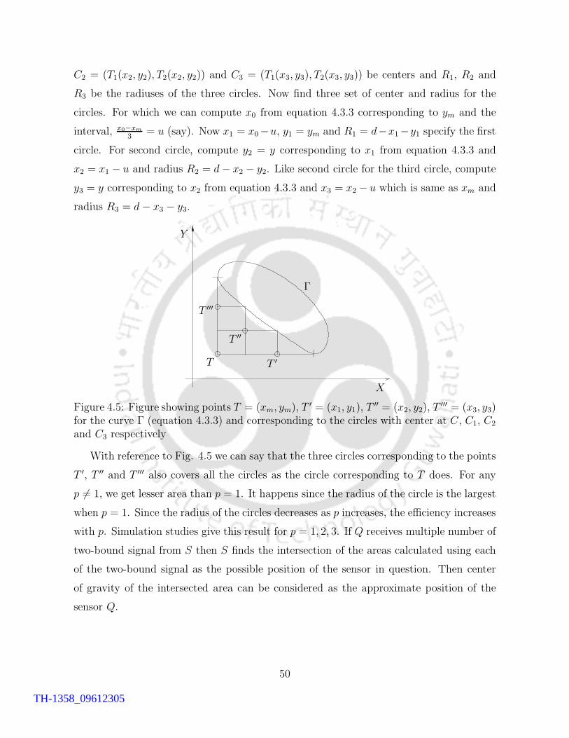
C2 = (T1(x2, y2), T2(x2, y2)) and C3 = (T1(x3, y3), T2(x3, y3)) be centers and R1, R2 and
R3 be the radiuses of the three circles. Now find three set of center and radius for the
circles. For which we can compute x0 from equation 4.3.3 corresponding to ym and the
interval, x0−xm
3= u (say). Now x1 = x0−u, y1 = ym and R1 = d−x1−y1 specify the first
circle. For second circle, compute y2 = y corresponding to x1 from equation 4.3.3 and
x2 = x1 − u and radius R2 = d− x2 − y2. Like second circle for the third circle, compute
y3 = y corresponding to x2 from equation 4.3.3 and x3 = x2 − u which is same as xm and
radius R3 = d− x3 − y3.
Γ
T T ′
T ′′
T ′′′
X
Y
Figure 4.5: Figure showing points T = (xm, ym), T′ = (x1, y1), T
′′ = (x2, y2), T′′′ = (x3, y3)
for the curve Γ (equation 4.3.3) and corresponding to the circles with center at C, C1, C2
and C3 respectively
With reference to Fig. 4.5 we can say that the three circles corresponding to the points
T ′, T ′′ and T ′′′ also covers all the circles as the circle corresponding to T does. For any
p 6= 1, we get lesser area than p = 1. It happens since the radius of the circle is the largest
when p = 1. Since the radius of the circles decreases as p increases, the efficiency increases
with p. Simulation studies give this result for p = 1, 2, 3. If Q receives multiple number of
two-bound signal from S then S finds the intersection of the areas calculated using each
of the two-bound signal as the possible position of the sensor in question. Then center
of gravity of the intersected area can be considered as the approximate position of the
sensor Q.
50
TH-1358_09612305
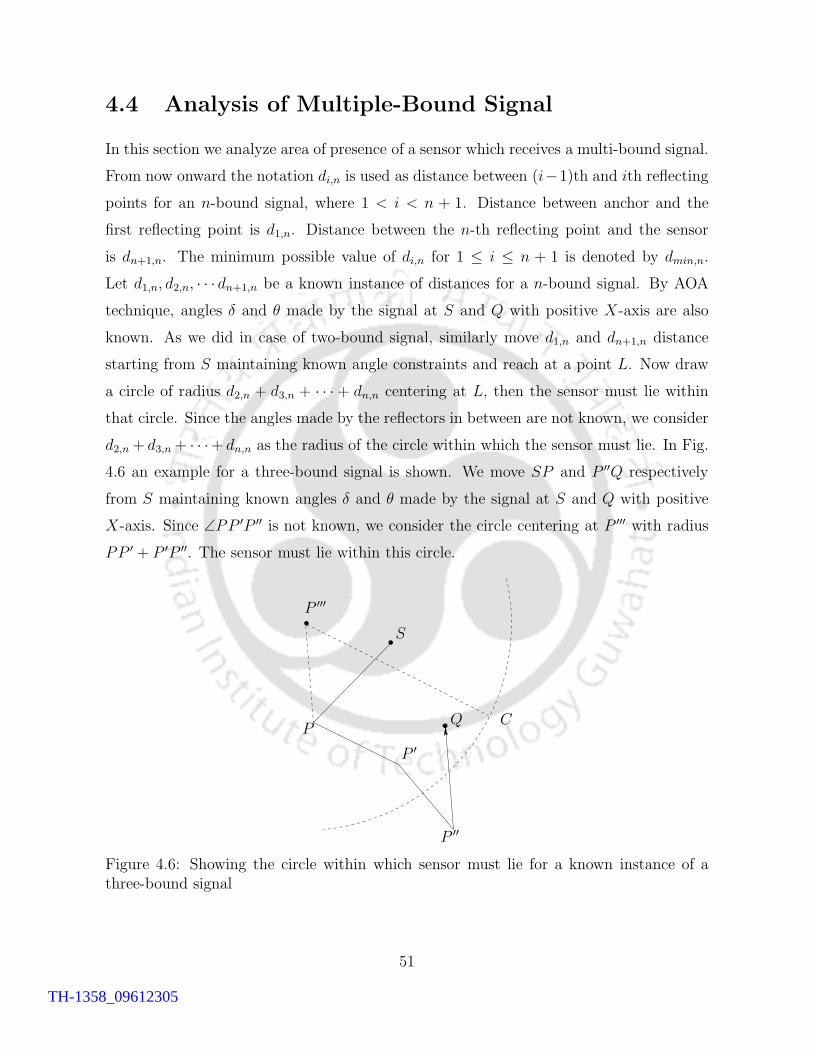
4.4 Analysis of Multiple-Bound Signal
In this section we analyze area of presence of a sensor which receives a multi-bound signal.
From now onward the notation di,n is used as distance between (i−1)th and ith reflecting
points for an n-bound signal, where 1 < i < n + 1. Distance between anchor and the
first reflecting point is d1,n. Distance between the n-th reflecting point and the sensor
is dn+1,n. The minimum possible value of di,n for 1 ≤ i ≤ n + 1 is denoted by dmin,n.
Let d1,n, d2,n, · · · dn+1,n be a known instance of distances for a n-bound signal. By AOA
technique, angles δ and θ made by the signal at S and Q with positive X-axis are also
known. As we did in case of two-bound signal, similarly move d1,n and dn+1,n distance
starting from S maintaining known angle constraints and reach at a point L. Now draw
a circle of radius d2,n + d3,n + · · · + dn,n centering at L, then the sensor must lie within
that circle. Since the angles made by the reflectors in between are not known, we consider
d2,n + d3,n + · · ·+ dn,n as the radius of the circle within which the sensor must lie. In Fig.
4.6 an example for a three-bound signal is shown. We move SP and P ′′Q respectively
from S maintaining known angles δ and θ made by the signal at S and Q with positive
X-axis. Since ∠PP ′P ′′ is not known, we consider the circle centering at P ′′′ with radius
PP ′ + P ′P ′′. The sensor must lie within this circle.
P
P ′
P ′′
P ′′′
Q
S
C
Figure 4.6: Showing the circle within which sensor must lie for a known instance of athree-bound signal
51
TH-1358_09612305
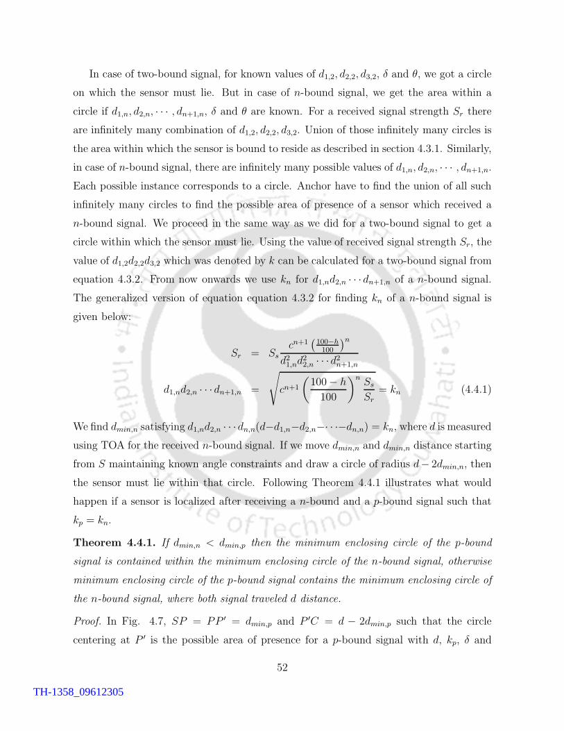
In case of two-bound signal, for known values of d1,2, d2,2, d3,2, δ and θ, we got a circle
on which the sensor must lie. But in case of n-bound signal, we get the area within a
circle if d1,n, d2,n, · · · , dn+1,n, δ and θ are known. For a received signal strength Sr there
are infinitely many combination of d1,2, d2,2, d3,2. Union of those infinitely many circles is
the area within which the sensor is bound to reside as described in section 4.3.1. Similarly,
in case of n-bound signal, there are infinitely many possible values of d1,n, d2,n, · · · , dn+1,n.
Each possible instance corresponds to a circle. Anchor have to find the union of all such
infinitely many circles to find the possible area of presence of a sensor which received a
n-bound signal. We proceed in the same way as we did for a two-bound signal to get a
circle within which the sensor must lie. Using the value of received signal strength Sr, the
value of d1,2d2,2d3,2 which was denoted by k can be calculated for a two-bound signal from
equation 4.3.2. From now onwards we use kn for d1,nd2,n · · · dn+1,n of a n-bound signal.
The generalized version of equation equation 4.3.2 for finding kn of a n-bound signal is
given below:
Sr = Ss
cn+1(
100−h100
)n
d21,nd22,n · · ·d2n+1,n
d1,nd2,n · · · dn+1,n =
√
cn+1
(
100− h
100
)nSs
Sr= kn (4.4.1)
We find dmin,n satisfying d1,nd2,n · · · dn,n(d−d1,n−d2,n−· · ·−dn,n) = kn, where d is measured
using TOA for the received n-bound signal. If we move dmin,n and dmin,n distance starting
from S maintaining known angle constraints and draw a circle of radius d− 2dmin,n, then
the sensor must lie within that circle. Following Theorem 4.4.1 illustrates what would
happen if a sensor is localized after receiving a n-bound and a p-bound signal such that
kp = kn.
Theorem 4.4.1. If dmin,n < dmin,p then the minimum enclosing circle of the p-bound
signal is contained within the minimum enclosing circle of the n-bound signal, otherwise
minimum enclosing circle of the p-bound signal contains the minimum enclosing circle of
the n-bound signal, where both signal traveled d distance.
Proof. In Fig. 4.7, SP = PP ′ = dmin,p and P ′C = d − 2dmin,p such that the circle
centering at P ′ is the possible area of presence for a p-bound signal with d, kp, δ and
52
TH-1358_09612305
θ. Let dmin,n < dmin,p. In Fig. 4.7, SL = LL′ = dmin,n. Now, L′C = L′P ′ + P ′C <
L′T +TP ′+P ′C = (dmin,p−dmin,n)+(dmin,p−dmin,n)+(d−2dmin,p) = d−2dmin,n = L′C ′.
So, the circle centering at L′ with radius d − 2dmin,n contains the point C, which is the
furthest point from L′ among the points on the circle centering at P ′. Hence, the circle of
the n-bound signal contains that of p-bound signal. Now, let dmin,n ≥ dmin,p. Following
similar logic, the minimum enclosing circle of the p-bound signal contains that of n-bound
signal.
T
S
P
P ′
L
L′
CC ′
Figure 4.7: Showing possible area of presence for a p-bound signal and of a n-bound signal
Lemma 4.4.2. Maximum possible value of kn−1 is equal to(
dn
)nwhere d1,n−1 d2,n−1 · · ·
dn−1,n−1 (d− d1,n−1 − · · · − dn−1,n−1) = kn−1 and di > 0 for all i = 1 to n− 1.
Proof. Consider the function f = d1,n−1d2,n−1...dn−1,n−1(d−d1,n−1−d2,n−1−· · ·−dn−1,n−1).
We have to find the values of di,n−1, for which f attains maximum. f ′(di,n−1) = 0 implies
d = di,n−1 + (d1,n−1 + d2,n−1 + · · · + dn−1,n−1) for all i, which implies di,n−1 = dnfor all
i. f ′′(di,n−1) < 0 implies f attains maximum when di,n−1 = dnand hence the maximum
value of kn−1 is(
dn
)n.
Lemma 4.4.3. If dmin,n−1 = di,n−1 for some i in the equation d1,n−1 · · · dn−1,n−1(d −d1,n−1 − · · · − dn−1,n−1) = kn−1, then dj,n−1 =
d−dmin,n−1
n−1for all j 6= i.
Proof. Without loss of generality let d1,n−1 = dmin,n−1. So, d2,n−1 · · · dn−1,n−1dn,n−1 =kn−1
dmin,n−1. Now consider g = d2,n−1 · · · dn−1,n−1dn,n−1, where d2,n−1+· · ·+dn−1,n−1+dn,n−1 =
53
TH-1358_09612305

d− dmin,n−1. Using Lemma 4.4.2, we can say, g attains maximum when d2,n−1 = d3,n−1 =
· · · = dn−1,n−1 = dn,n−1 =d−dmin,n−1
n−1and maximum value of g =
[
d−dmin,n−1
n−1
]n−1
. Clearly
dmin,n−1 ∈(
0, dn
]
. So,[
d−dmin,n−1
n−1
]n−1
≥ kn−1
dmin,n−1. Consider function h(c) = c
[
d−cn−1
]n−1.
h′(c) ≥ 0 implies h is increasing ∈(
0, dn
]
. If dmin,n−1
[
d−dmin,n−1
n−1
]n−1
= kn−1, then the
lemma is proved. Else if dmin,n−1
[
d−dmin,n−1
n−1
]n−1
> kn−1, then the property of function h
implies that dmin,n−1 can not be the minimum, which is a contradiction. Hence proved.
Lemma 4.4.4. There may not exist a p-bound signal with same d and kn of a n-bound
signal and vice versa.
Proof. If p is such that kn >(
dp+1
)p+1
, then using Lemma 4.4.2, we can say that for those
values of d and kn a p-bound signal can not exist. The other part is similar.
For example we can find d and k2 corresponding to a two-bound signal, such that a
three-bound signal cannot exist. Such values of d must satisfy the inequality(
d3
)3>
(
d4
)4,
which implies d < 25627
= 9.48. So, for d < 9.48 and k2 >(
d4
)4, no three-bound signal can
exist.
Theorem 4.4.5. The minimum enclosing circle of a n-bound signal is contained within
the minimum enclosing circle of a p-bound signal (p > n) if both the signals have same d
and kn = kp with d > (p+ 1)(
pn
)n
p−n .
Proof. We can write dmin,p
(
d−dmin,p
p
)p
= kp using Lemma 4.4.3. Let
H(n) = dmin,p
(
d− dmin,p
p
)p
− dmin,p
(
d− dmin,p
n
)n
= dmin,p (d− dmin,p)n
(
(d− dmin,p)p−n
pp− 1
nn
)
If d > dmin,p + p(
pn
)n
p−n then H(n) > 0.
Since dmin,p ∈(
0, dp+1
]
H(n) > 0 if d > (p+ 1)(p
n
)n
p−n
(4.4.2)
54
TH-1358_09612305
Again H(n) > 0 implies k = dmin,p
(
d−dmin,p
p
)p
> dmin,p
(
d−dmin,p
n
)n
. Since f(x) =
x(
d−xn
)nis an increasing function for x ∈
(
0, dn+1
]
, there exists x > dmin,p such that
x(
d−xn
)n= kn. Using Lemma 4.4.3, x = dmin,n. Finally,
H(n) > 0 implies dmin,n > dmin,p (4.4.3)
So, dmin,n > dmin,p for all d > (p + 1)(
pn
)n
p−n . Using Theorem 4.4.1, we can conclude
that the minimum enclosing circle of a n-bound signal is contained within the minimum
enclosing circle of a p-bound signal if both the signals have same d and kp = kn with
d > (p+ 1)(
pn
)n
p−n .
4.5 Area of Presence for an Unknown-Bound Signal
Practically it is not possible to know the actual value of n of a received n− bound signal.
Hence we can not calculate kn for unknown n (Ref. equation 4.4.1). In this section we
analyze and find conditions on d such that localizing a sensor is possible after receiving
any n-bound signal, where n is unknown, using received signal strength Sr. However, we
assume that the value N , of maximum possible bound in the system is known.
Theorem 4.5.1. For a n-bound signal (n ≤ N), the sensor lies within a circle calculated
assuming the signal is N-bound if d ≥ (N + 1)(
N+1N
)N√
c(100−h)100
.
Proof. Let a sensor receives a signal with signal strength Sr and let distance traveled by
the signal be d, measured by TOA technique. The number of bounds for the signal is
not known to the receiver. Let originally the received signal be a n-bound signal. We
can establish the following relation using equation 4.4.1, assuming that it is a N -bound
signal,
kN = kn
(
c(100− h)
100
)N−n
2
(4.5.1)
Using Lemma 4.4.2, if kN ≤(
dN+1
)N+1, then for the signal, nmay be equal to N . So, there
exists dmin,N such that dmin,N
(
d−dmin,N
N
)N
= kN . We find a range of d such that kN ≤
55
TH-1358_09612305
(
dN+1
)N+1always occurs. From the equation 4.5.1 and Lemma 4.4.2, we can rewrite this
expression as(
dn+1
)n+1(
c(100−h)100
)N−n
2 ≤(
dN+1
)N+1, i.e., d ≥ (N +1)
(
N+1n+1
)( n+1
N−n)√
c(100−h)100
.
Since (N + 1)(
N+1n+1
)( n+1
N−n)√
c(100−h)100
is an increasing function for n = 1 to N − 1, we can
conclude if d ≥ (N + 1)(
N+1N
)N√
c(100−h)100
, then kN ≤(
dN+1
)N+1always occurs.
For the n-bound signal, there exist dmin,n such that dmin,n
(
d−dmin,n
n
)n
= kn. Let W (n)
be a function defined below:
W (n) = dmin,N
(
d− dmin,N
N
)N
−(
c(100− h)
100
)N−n
2
dmin,N
(
d− dmin,N
n
)n
= dmin,N(d− dmin,N)n
(d− dmin,N)N−n
NN−
(
c(100−h)100
)N−n
2
nn
If d ≥ dmin,N +N(
Nn
)n
N−n
√
c(100−h)100
then W (n) ≥ 0,
i.e., if d ≥ (N + 1)(
Nn
) nN−n
√
c(100−h)100
, then W (n) ≥ 0 since dmin,N ∈ (0, dN+1
].
As (N + 1)(
Nn
)n
N−n
√
c(100−h)100
is an increasing function for n = 1 to N − 1, we can
conclude if d ≥ (N + 1)(
NN−1
)N−1√
c(100−h)100
then W (n) ≥ 0.
Again, W (n) ≥ 0 implies dmin,N
(
(d−dmin,N )
N
)N
≥(
c(100−h)100
)N−n
2
dmin,N
(
(d−dmin,N )
n
)n
which implies kn ≥ dmin,N
(
d−dmin,N
n
)n
, using equation 4.5.1.
Since f(c) = c(
d−cn
)nis increasing in
(
0, dn+1
]
, kn ≥ dmin,N
(
d−dmin,N
n
)n
implies dmin,n ≥dmin,N . So, W (n) ≥ 0 implies that dmin,n ≥ dmin,N .
Again, (N + 1)(
N+1N
)N√
c(100−h)100
> (N + 1)(
NN−1
)N−1√
c(100−h)100
. So, we can conclude
if d ≥ (N + 1)(
N+1N
)N√
c(100−h)100
then minimum enclosing circle of any n-bound signal
where n ≤ N is contained within the minimum enclosing circle of a N -bound signal with
same received signal strength Sr.
56
TH-1358_09612305
4.6 Proposed Localization Algorithm
4.6.1 System model
All anchors are equipped with an omnidirectional antenna for sending beacons and also
a directional antenna for the measurement of AOA of a signal from other sensors. Other
sensors are equipped with directional antennas to avoid collision when it receives more
than one beacon from an anchor coming through different paths at different angles. An
anchor is said to be a neighbor of another anchor if it is located within twice the trans-
mission range of the second anchor. Anchors are synchronized with some global clock
(possibly through GPS) such that at a time only one anchor sends a beacon to avoid
collision with the beacons from the neighboring anchors. This ensures that a receiving
sensor receives only one beacon at a time from a particular anchor.
4.6.2 The algorithm
Based on the above discussions, Algorithm 2 (LocalizeSensor) given below finds the
position of a sensor Q using the beacon signals from an anchor S.
Algorithm 2 LocalizeSensor
1: Anchor S sends beacon by omnidirectional antenna with < anchor id > first, using electro-magnetic signal and second, using ultrasonic signal.
2: for each sensor Q who hears the beacons do3: Receives electromagnetic signal and measures receiving signal strength Sr.4: Measures the angles of arrival (θ) of the ultrasonic signal and transmits back <
sensor id, θ, Sr, φ > to S via the same path.5: end for
6: S measures the angles of arrival (δ) while receiving the reply and computes the correspondingdistances (d) traveled by the beacon by measuring the TOA.
7: Anchor computes the area of presence of the sensor according to section 4.5.8: If Q receives different signals then intersection of all such areas (calculated in the preceding
step) is the area of presence of Q.
57
TH-1358_09612305
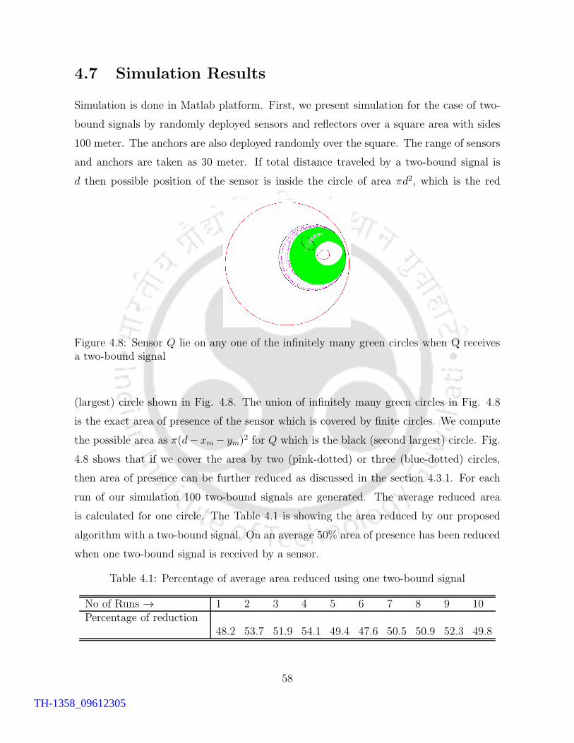
4.7 Simulation Results
Simulation is done in Matlab platform. First, we present simulation for the case of two-
bound signals by randomly deployed sensors and reflectors over a square area with sides
100 meter. The anchors are also deployed randomly over the square. The range of sensors
and anchors are taken as 30 meter. If total distance traveled by a two-bound signal is
d then possible position of the sensor is inside the circle of area πd2, which is the red
Figure 4.8: Sensor Q lie on any one of the infinitely many green circles when Q receivesa two-bound signal
(largest) circle shown in Fig. 4.8. The union of infinitely many green circles in Fig. 4.8
is the exact area of presence of the sensor which is covered by finite circles. We compute
the possible area as π(d− xm − ym)2 for Q which is the black (second largest) circle. Fig.
4.8 shows that if we cover the area by two (pink-dotted) or three (blue-dotted) circles,
then area of presence can be further reduced as discussed in the section 4.3.1. For each
run of our simulation 100 two-bound signals are generated. The average reduced area
is calculated for one circle. The Table 4.1 is showing the area reduced by our proposed
algorithm with a two-bound signal. On an average 50% area of presence has been reduced
when one two-bound signal is received by a sensor.
Table 4.1: Percentage of average area reduced using one two-bound signal
No of Runs → 1 2 3 4 5 6 7 8 9 10Percentage of reduction
48.2 53.7 51.9 54.1 49.4 47.6 50.5 50.9 52.3 49.8
58
TH-1358_09612305
Table 4.2: Reduction in average area compared to trilateration when sensor receives threetwo-bound signals
No of Runs → 1 2 3 4 5 6 7 8 9 10Percentage of reduction 34.2 37.7 32.1 41.3 33.2 39.8 42.2 37.2 30.4 30.9
Table 4.3: Error comparison when sensor receives three two-bound signals
No of Runs → 1 2 3 4 5 6 7 8 9 10Error in our technique(in meter)
3.7 4.8 3.1 3.1 3.7 3.9 3.3 2.9 3.2 3.8
Error in trilateration (inmeter)
5.3 6.9 6.2 5.2 8.0 6.2 6.4 4.6 6.5 6.4
Percentage of improve-ment
30.2 30.7 49.1 39.9 53.2 37.0 48.2 37.2 50.4 40.4
Table 4.4: Reduction in average area compared to trilateration when sensor receives threeunknown-bound signals
Maximum number of bounds → 3 4 5 6 7 8Percentage of reduction 24.54 14.7 8.6 6.1 4.5 4.1
Table 4.5: Error comparison when sensor receives three unknown-bound signals
Maximum number of bounds → 3 4 5 6 7 8Error in our technique (in meter) 8.17 9.60 10.19 9.70 7.28 10.76Error in trilateration (in meter) 9.45 10.16 10.46 9.80 7.33 10.78Percentage of improvement 13.54 5.49 2.63 1.00 0.60 0.25
59
TH-1358_09612305
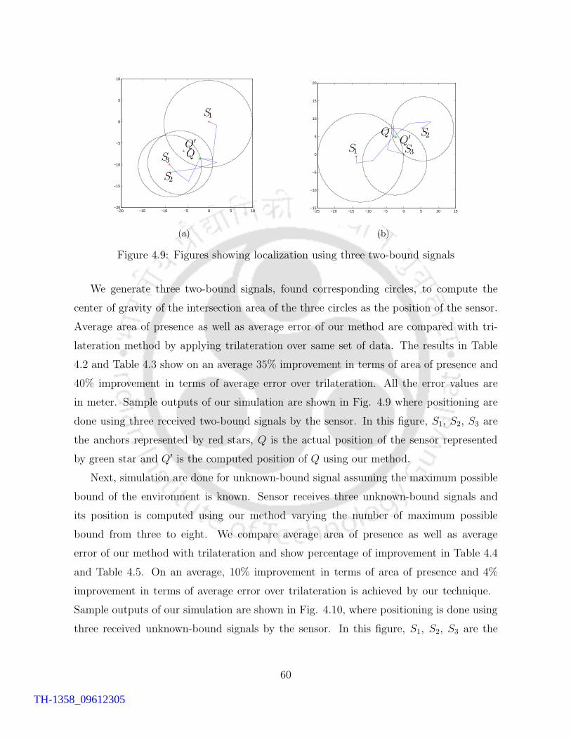
−20 −15 −10 −5 0 5 10−20
−15
−10
−5
0
5
10
Q
1
Q′
2
3
S
S
S
(a)
−25 −20 −15 −10 −5 0 5 10 15−15
−10
−5
0
5
10
15
20
Q
1
Q′ 2
3
S
SS
(b)
Figure 4.9: Figures showing localization using three two-bound signals
We generate three two-bound signals, found corresponding circles, to compute the
center of gravity of the intersection area of the three circles as the position of the sensor.
Average area of presence as well as average error of our method are compared with tri-
lateration method by applying trilateration over same set of data. The results in Table
4.2 and Table 4.3 show on an average 35% improvement in terms of area of presence and
40% improvement in terms of average error over trilateration. All the error values are
in meter. Sample outputs of our simulation are shown in Fig. 4.9 where positioning are
done using three received two-bound signals by the sensor. In this figure, S1, S2, S3 are
the anchors represented by red stars, Q is the actual position of the sensor represented
by green star and Q′ is the computed position of Q using our method.
Next, simulation are done for unknown-bound signal assuming the maximum possible
bound of the environment is known. Sensor receives three unknown-bound signals and
its position is computed using our method varying the number of maximum possible
bound from three to eight. We compare average area of presence as well as average
error of our method with trilateration and show percentage of improvement in Table 4.4
and Table 4.5. On an average, 10% improvement in terms of area of presence and 4%
improvement in terms of average error over trilateration is achieved by our technique.
Sample outputs of our simulation are shown in Fig. 4.10, where positioning is done using
three received unknown-bound signals by the sensor. In this figure, S1, S2, S3 are the
60
TH-1358_09612305
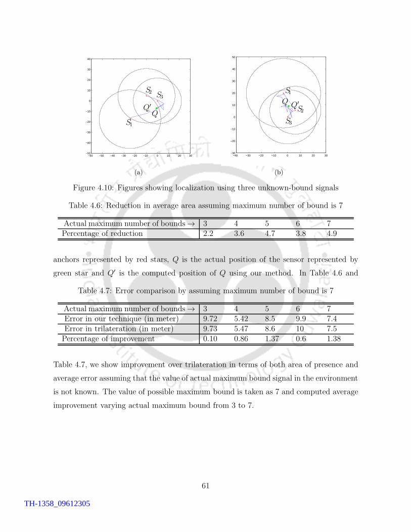
−60 −50 −40 −30 −20 −10 0 10 20 30−50
−40
−30
−20
−10
0
10
20
30
40
Q
1
Q′
23
S
SS
(a)
−40 −30 −20 −10 0 10 20 30−30
−20
−10
0
10
20
30
40
50
Q1
Q′2
3S
S
S
(b)
Figure 4.10: Figures showing localization using three unknown-bound signals
Table 4.6: Reduction in average area assuming maximum number of bound is 7
Actual maximum number of bounds→ 3 4 5 6 7Percentage of reduction 2.2 3.6 4.7 3.8 4.9
anchors represented by red stars, Q is the actual position of the sensor represented by
green star and Q′ is the computed position of Q using our method. In Table 4.6 and
Table 4.7: Error comparison by assuming maximum number of bound is 7
Actual maximum number of bounds→ 3 4 5 6 7Error in our technique (in meter) 9.72 5.42 8.5 9.9 7.4Error in trilateration (in meter) 9.73 5.47 8.6 10 7.5Percentage of improvement 0.10 0.86 1.37 0.6 1.38
Table 4.7, we show improvement over trilateration in terms of both area of presence and
average error assuming that the value of actual maximum bound signal in the environment
is not known. The value of possible maximum bound is taken as 7 and computed average
improvement varying actual maximum bound from 3 to 7.
61
TH-1358_09612305

4.8 Conclusions
In this work we have proposed a localization algorithm under a model where multiple-
bound (up to N -bound, any known N) signals are allowed. To the best of our knowledge
there is no deterministic algorithm for localization where the received multiple-bound
(more than one-bound) signals are used in absent of LOS signals. Comparison with
trilateration shows on an average 35% improvement when sensor receives three two-bound
signals from different anchors and on an average 10% improvement when sensor receives
three unknown-bound signals from different anchors in terms of area of presence. In future
we will try to solve the localization problem under a more practical model relaxing the
condition of known N and introducing measurement errors.
62
TH-1358_09612305
Chapter 5
Mobile Sensor Localization using
Static Anchor under Constrained
Motion
5.1 Introduction
Mobile wireless sensor networks (MWSNs) is a recent development of WSNs. In MWSN
mobile sensors are needed to be localized in such a way that their position can be known
at any time instant. This work is motivated by the beacon point selection strategy used in
[46, 75, 84] for static sensor localization using mobile anchors. In all these three schemes
since static sensors receive beacons from mobile anchors, sensors know the co-ordinates of
the beacon points. Hence chord formed by two beacon points is unique in [75]. Similarly
unique circular lamina with known equations of the circles can be formed using a beacon
point in [46]. Contrary to that in our proposed algorithm, as anchors are static and mobile
sensors are receiving beacons at different positions, so co-ordinate of beacon points are
not known and a unique chord can not be formed using two beacon points. Hence we use
communication circles of two different anchors to identify the chord and localize the mobile
sensor in proposed Algorithm 3. We modify the definition of beacon point accordingly and
propose range-free deterministic localization algorithms under different circumstances.
63
TH-1358_09612305
5.1.1 Our contribution
According to our proposed algorithm LWCD, a mobile sensor can localize itself within any
predefined error bound when it passes through communication circles of two different an-
chors. As it passes through more communication circles, positioning error can be further
reduced. Simulation results of LWCD show around 75% improvement of the positioning
error over the existing algorithm [90]. When mobile sensor passes through three and five
more communication circles, 40% and 55% further reduction in error are shown respec-
tively. In presence of obstacles, our proposed algorithm LWCDPO can localize mobile
sensors within same error bound as LWCD.
The rest of the chapter is organized as follows. We propose a localization algorithm
LWCD assuming mobile sensor does not change its direction during movement in section
5.2. With the same assumption, we propose another algorithm LWCDPO to localize
mobile sensors in presence of obstacles in section 5.3. The simulation results of our
algorithms are presented in section 5.4, along with performance comparison with relevant
algorithms. Finally we conclude in section 5.5.
5.2 Localization without Change of Direction
In this section we propose a mobile sensor localization algorithm assuming sensors do not
change their direction during localization. System model for the algorithm is given below.
5.2.1 System model
Static anchors with equal communication range are deployed sparsely in a two dimensional
plane. All mobile sensors have the information about the communication range of the
anchors. Also mobile sensors and anchors have equal communication range r. Anchors
are identified by their locations. The anchors periodically broadcast beacons with their
locations. The time interval between two consecutive broadcasts of beacons is t, which is
fixed and same for all anchors. The mobile sensors move according to the requirement of
underlying application. During localization phase, mobile sensors move with a uniform
velocity until localization.
64
TH-1358_09612305
When a mobile sensor receives first beacon from an anchor, it recognizes that it is
in the communication range of that anchor. The position of receiving first beacon is an
approximate end point of the chord of the communication circle of that anchor, along
which it is moving. Similarly, the position of receiving the last beacon from that anchor
denotes the approximate position of the other end point of that chord. As mobile sensor
does not know the positions of receiving beacons, it records the time of receiving the first
and last beacon according to it’s own clock to calculate the approximate chord length.
We denote the time of receiving any beacon according to the sensor’s clock as the time
stamp of the beacon. Definition of the key terms used in this paper are given below.
Definition 5.2.1. (Beacon distance) Distance traveled by the mobile sensor between
receiving two consecutive beacons from an anchor is called beacon distance.
The beacon distance is denoted by u and is equal to vt, where v is uniform velocity
of the mobile sensor during localization and t is time interval of periodical broadcasts of
beacon by the anchor.
Definition 5.2.2. (Beacon point) Beacon received by a mobile sensor from an anchor at
time x is marked as a beacon point by the sensor if and only if the sensor does not receive
any beacon either in time interval [x− t0, x) or in time interval (x, x+ t0] from the same
anchor, where t < t0 < 2t and t is time interval of periodical broadcasts of beacon by the
anchor.
Definition 5.2.3. (Communication circle) The circle with radius r centering at an anchor,
where r is the communication range of the anchor.
Beacon distance should be much lesser than communication range in order to receive
a good number of beacons. When a mobile sensor moves into the transmission area of
an anchor and receives a beacon, it knows the equation of the communication circle in
which it is moving since the communication range and position of the anchor is known.
We call the line along which a mobile sensor is moving within a communication circle as
it’s actual line of movement. The mobile sensors are equipped with a electronic compass
[65] for knowing the direction of movement and a timer to record the time stamps of the
received beacons. Electronic compass yields an in-plane heading accuracy of ±1 degree
[65].
65
TH-1358_09612305
5.2.2 Beacon list
Each mobile sensor maintains a beacon list with two columns. Each entry of the list
contains time stamp (time stamp) of the received beacon and corresponding anchor id
(anchor id) according to it’s own clock. When a mobile sensor receives a beacon from
an anchor, it records < time stamp, anchor id > in the beacon list. Here a beacon is
represented as < time stamp, anchor id >. At the beginning, list is empty. Let a sensor
receives a beacon from an anchor with anchor id = i. It records < time stamp, i > in the
first column and marks it as a beacon point. If another beacon is received from the same
anchor by time t0 then sensor replaces the last beacon with latest one provided the last
beacon is not marked as beacon point. If last beacon is marked as beacon point then it
adds this beacon in the same column. If no beacon is received by the time t0 then the last
beacon is marked as beacon point. A sensor may receive many beacons but the beacons
marked by above rule, are the beacon points. In between whenever any beacon comes
from a different anchor with anchor id = j, say, (j 6= i), it records < time stamp, j >
in the second column and marks it as a beacon point. If both the columns are non-
empty and a beacon is received from an anchor with anchor id = s (s 6= i, j), then that
beacon is ignored. Following the procedure discussed above, sensor records at most two
beacon points for each anchor. There is possibility of receiving only one beacon from an
anchor, in that case only one beacon point appears in a column of the list. So, there can
be maximum of four entries in the list. After localizing itself, the sensor deletes those
marked beacon points to make the list empty, as explained in section 5.2.6.
S
M PP
P ′P ′1
1 2
2
Figure 5.1: Showing two possible lines of movement including the actual one (P1P2)
66
TH-1358_09612305
5.2.3 Finding line of movement
We explain how a mobile sensor can identify its actual line of movement based on beacon
points corresponding to two anchors. A mobile sensor calculates the time difference
between receiving two beacon points from an anchor, to calculate the chord length 2l.
Using the electronic compass, the sensor also knows the gradient of the line along which
it moves. As there exist only two possible chords of same length and gradient in a circle,
the sensor is moving along any one of those two lines (Ref. Fig. 5.1). For simplicity, let the
sensor moves along a line parallel to X-axis. Throughout the chapter, in the figures, filled
circles denote beacon points and unfilled circles denote received beacons except beacon
points, on the line of movement of a mobile sensor.
Let one anchor be placed at S = (0, 0) and P1P2 is the actual line of movement of the
mobile sensor, where filled circles labeled as P1 and P2 are the beacon points as shown in
Fig. 5.1. The equation of the communication circle is x2 + y2 = r2 and SM =√r2 − l2,
where P1P2 = 2l. Hence, the possible line of movement of the mobile sensor is either P1P2
or P ′1P
′2, whose equations are y = ±
√r2 − l2. More information is needed to identify
the actual line. For which the sensor continues its movement along the same line until it
crosses the communication circle of another anchor. Let S ′ = (a, b), b 6= 0 be a different
anchor as shown in Fig. 5.2. Let P3, P4 be the beacon points corresponding to S ′ and
S ′M ′ =√r2 − l′2, where P3P4 = 2l′. Similarly, the possible line of movement of the
mobile sensor is either P3P4 or P′3P
′4, whose equations are y = b±
√r2 − l′2. Now, among
these four lines, equations of two lines should be same with the actual line of movement,
since there is exactly one line along which the sensor is moving. According to Fig. 5.2,
the equation of the actual line is y =√r2 − l2 i.e., y = b+
√r2 − l′2.
Using the selected equation of the line of movement, the sensor can calculate the coordi-
nates of the points P1, P2, P3, P4. Current position of the mobile sensor can be calculated
based on any Pi for i = 1 to 4, and elapsed time from timer. To localize itself, a sensor
has to pass through communication circles of two different anchors where the line joining
those two anchors should not be parallel with the line of the sensor, i.e., SS ′ ∦ P1P4.
67
TH-1358_09612305
S
S ′
P PPP
P ′
P ′ P ′
P ′
1
1 2
2
3
3
4
4
Figure 5.2: Two communication circles are required to find the correct line of movement
5.2.4 Error analysis
The above technique of choosing the line of movement among four calculated chords is
not applicable for finding actual line of movement unless beacon points are located on
the perimeter of the communication circles of the respective anchors. In practice beacon
points, C, C ′ marked with filled circles (Ref. Fig. 5.3) may lie inside the communication
circles due to periodic broadcast of anchors. This may lead to a situation where equation
of no two chords are common. In that case mobile sensor finds approximate line of
movement instead of actual one. Hence localization error occurs.
Again, P1C ≤ u and P2C′ ≤ u, where P1 and P2 are the points of intersection of the
actual line of movement of the mobile sensor with communication circle of the anchor S.
For some h1, h2 ∈ [0, 1], we can write
P1C = h1u
P2C′ = h2u (5.2.1)
According to Fig. 5.3, possible approximate lines of movement are P ′1P
′2 and P ′′
1 P′′2 . Mobile
sensor can measure the length CC ′ from its velocity and time stamps of the beacon points.
The sensor misinterprets the length CC ′ as the length of the chords P1P2 along which
it is moving. So, the actual line of movement P1P2 is projected to the approximate line
of movement P ′1P
′2 such that CC ′ = P ′
1P′2. Due to the symmetric nature of circle, we
68
TH-1358_09612305
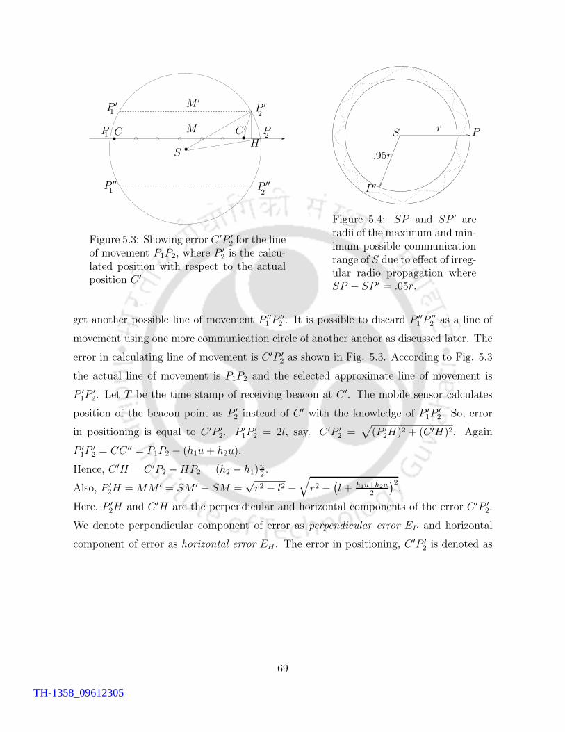
1
1
1
2
2
2
M
M ′
PPH
P ′P ′
P ′′P ′′
C C ′
S
Figure 5.3: Showing error C ′P ′2 for the line
of movement P1P2, where P ′2 is the calcu-
lated position with respect to the actualposition C ′
P
P ′
S r
.95r
Figure 5.4: SP and SP ′ areradii of the maximum and min-imum possible communicationrange of S due to effect of irreg-ular radio propagation whereSP − SP ′ = .05r.
get another possible line of movement P ′′1 P
′′2 . It is possible to discard P ′′
1 P′′2 as a line of
movement using one more communication circle of another anchor as discussed later. The
error in calculating line of movement is C ′P ′2 as shown in Fig. 5.3. According to Fig. 5.3
the actual line of movement is P1P2 and the selected approximate line of movement is
P ′1P
′2. Let T be the time stamp of receiving beacon at C ′. The mobile sensor calculates
position of the beacon point as P ′2 instead of C ′ with the knowledge of P ′
1P′2. So, error
in positioning is equal to C ′P ′2. P ′
1P′2 = 2l, say. C ′P ′
2 =√
(P ′2H)2 + (C ′H)2. Again
P ′1P
′2 = CC ′′ = P1P2 − (h1u+ h2u).
Hence, C ′H = C ′P2 −HP2 = (h2 − h1)u2.
Also, P ′2H = MM ′ = SM ′ − SM =
√r2 − l2 −
√
r2 −(
l + h1u+h2u2
)2.
Here, P ′2H and C ′H are the perpendicular and horizontal components of the error C ′P ′
2.
We denote perpendicular component of error as perpendicular error EP and horizontal
component of error as horizontal error EH . The error in positioning, C ′P ′2 is denoted as
69
TH-1358_09612305
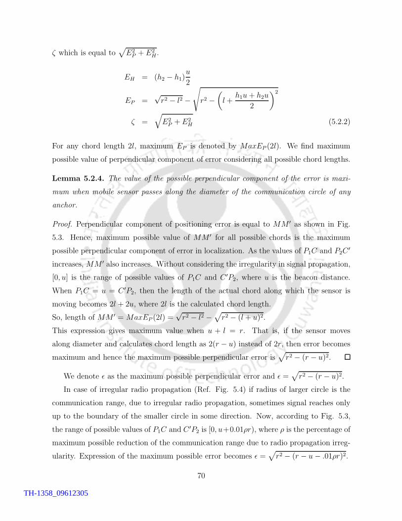
ζ which is equal to√
E2P + E2
H .
EH = (h2 − h1)u
2
EP =√r2 − l2 −
√
r2 −(
l +h1u+ h2u
2
)2
ζ =√
E2P + E2
H (5.2.2)
For any chord length 2l, maximum EP is denoted by MaxEP (2l). We find maximum
possible value of perpendicular component of error considering all possible chord lengths.
Lemma 5.2.4. The value of the possible perpendicular component of the error is maxi-
mum when mobile sensor passes along the diameter of the communication circle of any
anchor.
Proof. Perpendicular component of positioning error is equal to MM ′ as shown in Fig.
5.3. Hence, maximum possible value of MM ′ for all possible chords is the maximum
possible perpendicular component of error in localization. As the values of P1C and P2C′
increases, MM ′ also increases. Without considering the irregularity in signal propagation,
[0, u] is the range of possible values of P1C and C ′P2, where u is the beacon distance.
When P1C = u = C ′P2, then the length of the actual chord along which the sensor is
moving becomes 2l + 2u, where 2l is the calculated chord length.
So, length of MM ′ = MaxEP (2l) =√r2 − l2 −
√
r2 − (l + u)2.
This expression gives maximum value when u + l = r. That is, if the sensor moves
along diameter and calculates chord length as 2(r − u) instead of 2r, then error becomes
maximum and hence the maximum possible perpendicular error is√
r2 − (r − u)2.
We denote ε as the maximum possible perpendicular error and ε =√
r2 − (r − u)2.
In case of irregular radio propagation (Ref. Fig. 5.4) if radius of larger circle is the
communication range, due to irregular radio propagation, sometimes signal reaches only
up to the boundary of the smaller circle in some direction. Now, according to Fig. 5.3,
the range of possible values of P1C and C ′P2 is [0, u+0.01ρr), where ρ is the percentage of
maximum possible reduction of the communication range due to radio propagation irreg-
ularity. Expression of the maximum possible error becomes ε =√
r2 − (r − u− .01ρr)2.
70
TH-1358_09612305
We can keep ε under control by choosing appropriate values of u and r. For our sim-
ulation study we consider ρ = 5 in section 5.4. Simulation results are also shown varying
ρ from 0 to 20. However, if ρ is not known, it can be estimated by sending radio signals
and measuring the maximum and minimum communication ranges of environments. In a
dynamic environment when the radio irregularity changes frequently and sensor node also
moves out quickly from the communication range of the anchor, it is not easy to estimate
ρ perfectly because of low number of sampling. But in such a dynamic environment, in-
stead of online estimation of ρ, we can use minimum communication range for maximum
value of ρ i.e., the maximum possible radio irregularity of the environment. The upper
bound of ρ could be estimated off line with large sample for such a dynamic environment.
Now error in localization is less than the maximum of
√
ε2 +(
(h2−h1)u2
)2
, for all
h1, h2 ∈ [0, 1] (according to equation 5.2.2). Error ζ , is less than√
ε2 +(
u2
)2. But this is
an upper bound of ζ . We now find the least upper bound of ζ in the following lemma.
Lemma 5.2.5. Least upper bound of ζ is ε.
Proof. For any calculated chord length 2l, the horizontal component of error is EH =
|h2 − h1|u2 (Ref. equation 5.2.2). Let |h2 − h1| = f . So f ∈ [0, 1]. If horizontal error is
nonzero then f > 0. Then value of horizontal error is fu2. Without loss of generality, let
h2 = h1+f . Perpendicular error increases as h1+h2 increases, i.e., calculated chord length
decreases. So, maximum possible value of h1 = 1 − f and h2 = 1. Hence using equation
5.2.2, for any l, perpendicular error becomes EP =√r2 − l2 −
√
r2 −(
l + (2−f)u2
)2
.
From Lemma 5.2.4, for any f , EP is maximum when the original line passes along the
diameter, i.e., l + (2−f)u2
= r. So, for any f , ζ also attains maximum if l + (2−f)u2
= r and
the expression of maximum value of ζ becomes
√
r2 −(
r − (2−f)u2
)2
+ (uf2)2, which is a
decreasing function of f ∈ (0, 1].
Using limit of function and existence of
√
r2 −(
r − (2−f)u2
)2
+ (uf2)2 at f = 0, we can say,
it attains maximum at f = 0 i.e., least upper bound of error ζ is√
r2 − (r − u)2 = ε.
The value of maximum possible error is ε if we can select the line of movement which
is closer to the original line of movement among two calculated lines of movement. An
interesting observation is that if there is any error while selecting the line of movement,
71
TH-1358_09612305
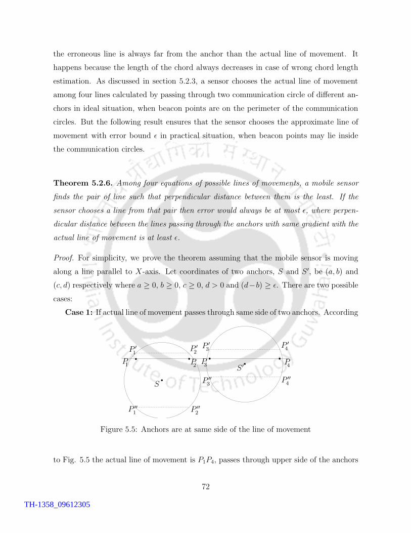
the erroneous line is always far from the anchor than the actual line of movement. It
happens because the length of the chord always decreases in case of wrong chord length
estimation. As discussed in section 5.2.3, a sensor chooses the actual line of movement
among four lines calculated by passing through two communication circle of different an-
chors in ideal situation, when beacon points are on the perimeter of the communication
circles. But the following result ensures that the sensor chooses the approximate line of
movement with error bound ε in practical situation, when beacon points may lie inside
the communication circles.
Theorem 5.2.6. Among four equations of possible lines of movements, a mobile sensor
finds the pair of line such that perpendicular distance between them is the least. If the
sensor chooses a line from that pair then error would always be at most ε, where perpen-
dicular distance between the lines passing through the anchors with same gradient with the
actual line of movement is at least ε.
Proof. For simplicity, we prove the theorem assuming that the mobile sensor is moving
along a line parallel to X-axis. Let coordinates of two anchors, S and S ′, be (a, b) and
(c, d) respectively where a ≥ 0, b ≥ 0, c ≥ 0, d > 0 and (d−b) ≥ ε. There are two possible
cases:
Case 1: If actual line of movement passes through same side of two anchors. According
PP PP
P ′P ′P ′ P ′
P ′′
P ′′
P ′′
P ′′
S
S ′
1
1
1
2
2
2
3
3
3
4
4
4
Figure 5.5: Anchors are at same side of the line of movement
to Fig. 5.5 the actual line of movement is P1P4, passes through upper side of the anchors
72
TH-1358_09612305
S and S ′. Let equation of the actual line of movement which passes through both the
circles be
y = dk where k ≥ 1 (5.2.3)
Let the chord length corresponding to the communication circles of the anchors S and S ′
be 2l and 2l′ respectively. Sensor calculates equation of the line P ′1P
′2 and P ′′
1 P′′2 as,
y = dk +MaxEP (2l)
q1where q1 ≥ 1 and (5.2.4)
y = 2b− dk − MaxEP (2l)
q1where q1 ≥ 1 (5.2.5)
respectively. Similarly, sensor calculates equation of the line P ′3P
′4 and P ′′
3 P′′4 as
y = dk +MaxEP (2l
′)
q2where q2 ≥ 1 and (5.2.6)
y = 2d− dk − MaxEP (2l′)
q2where q2 ≥ 1 (5.2.7)
respectively. Distance between the lines (equation 5.2.4 and equation 5.2.6) is equal to∣
∣
∣
MaxEP (2l′)q2
− MaxEP (2l)q1
∣
∣
∣≤ max
(
MaxEP (2l)q1
, MaxEP (2l′)q2
)
.
We denote distance between lines (equation 5.2.i) and (equation 5.2.j) byD(i, j) hereafter.
So, D(4, 6) ≤ max(
MaxEP (2l)q1
, MaxEP (2l′)q2
)
.
Let it be the smallest distance among those six possible distances D(i, j). If we choose
equation 5.2.4 or equation 5.2.6, we are choosing lines within max(
MaxEP (2l)q1
, MaxEP (2l′)q2
)
error, since D(3, 4) = MaxEP (2l)q1
as well as D(3, 6) = MaxEP (2l′)q2
. Actually we are finding
distances between correct line (equation 5.2.3) and the line we are choosing according to
our technique and checking it is less or equal to ε or not. Equation 5.2.4 and equation
5.2.6 make sure that there is at least one pair of lines whose perpendicular distance is less
than or equal to max(
MaxEP (2l)q1
, MaxEP (2l′)q2
)
.
Let D(4, 5) be the least. We have to check D(3, 5) only.
73
TH-1358_09612305
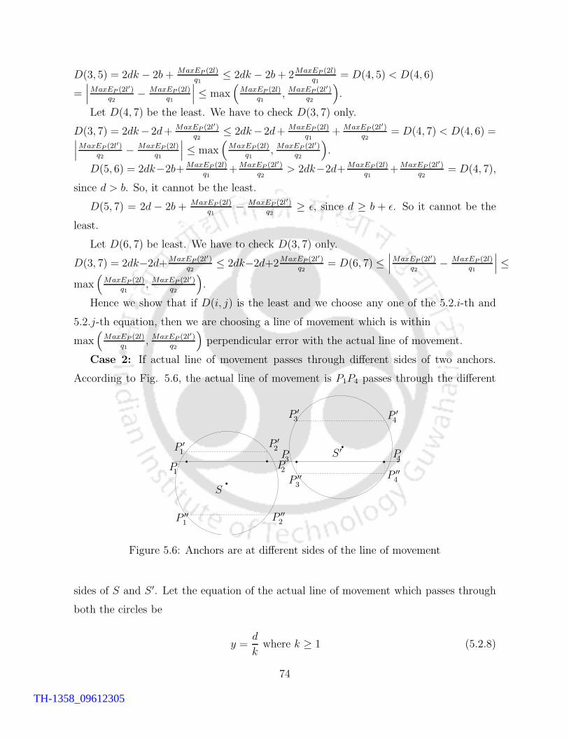
D(3, 5) = 2dk − 2b+ MaxEP (2l)q1
≤ 2dk − 2b+ 2MaxEP (2l)q1
= D(4, 5) < D(4, 6)
=∣
∣
∣
MaxEP (2l′)q2
− MaxEP (2l)q1
∣
∣
∣≤ max
(
MaxEP (2l)q1
, MaxEP (2l′)q2
)
.
Let D(4, 7) be the least. We have to check D(3, 7) only.
D(3, 7) = 2dk−2d+ MaxEP (2l′)q2
≤ 2dk−2d+ MaxEP (2l)q1
+ MaxEP (2l′)q2
= D(4, 7) < D(4, 6) =∣
∣
∣
MaxEP (2l′)q2
− MaxEP (2l)q1
∣
∣
∣≤ max
(
MaxEP (2l)q1
, MaxEP (2l′)q2
)
.
D(5, 6) = 2dk−2b+MaxEP (2l)q1
+MaxEP (2l′)q2
> 2dk−2d+MaxEP (2l)q1
+MaxEP (2l′)q2
= D(4, 7),
since d > b. So, it cannot be the least.
D(5, 7) = 2d − 2b + MaxEP (2l)q1
− MaxEP (2l′)q2
≥ ε, since d ≥ b + ε. So it cannot be the
least.
Let D(6, 7) be least. We have to check D(3, 7) only.
D(3, 7) = 2dk−2d+MaxEP (2l′)q2
≤ 2dk−2d+2MaxEP (2l′)q2
= D(6, 7) ≤∣
∣
∣
MaxEP (2l′)q2
− MaxEP (2l)q1
∣
∣
∣≤
max(
MaxEP (2l)q1
, MaxEP (2l′)q2
)
.
Hence we show that if D(i, j) is the least and we choose any one of the 5.2.i-th and
5.2.j-th equation, then we are choosing a line of movement which is within
max(
MaxEP (2l)q1
, MaxEP (2l′)q2
)
perpendicular error with the actual line of movement.
Case 2: If actual line of movement passes through different sides of two anchors.
According to Fig. 5.6, the actual line of movement is P1P4 passes through the different
P PPP
P ′P ′
P ′P ′
P ′′ P ′′
P ′′ P ′′
S
S ′
1
1
1 2
2
2
3
3
3
4
4
4
Figure 5.6: Anchors are at different sides of the line of movement
sides of S and S ′. Let the equation of the actual line of movement which passes through
both the circles be
y =d
kwhere k ≥ 1 (5.2.8)
74
TH-1358_09612305
Let the chord length corresponding to the communication circles of the anchors S and S ′
be 2l and 2l′ respectively. Sensor calculates equation of the line P ′1P
′2 and P ′′
1 P′′2 as,
y =d
k+
MaxEP (2l)
q1where q1 ≥ 1 and (5.2.9)
y = 2b− d
k− MaxEP (2l)
q1where q1 ≥ 1 (5.2.10)
respectively. Similarly, sensor calculates equation of the line P ′3P
′4 and P ′′
3 P′′4 as,
y =d
k− MaxEP (2l
′)
q2where q2 ≥ 1 and (5.2.11)
y = 2d− d
k+
MaxEP (2l′)
q2where q2 ≥ 1 (5.2.12)
respectively. Now perpendicular distance between equation 5.2.9 and equation 5.2.11 is
equal to∣
∣
∣
MaxEP (2l′)q2
+ MaxEP (2l)q1
∣
∣
∣≤ 2max
(
MaxEP (2l)q1
, MaxEP (2l′)q2
)
.
So, D(9, 11) = MaxEP (2l)q1
+ MaxEP (2l′)q2
≤ 2max(
MaxEP (2l)q1
, MaxEP (2l′)q2
)
.
Let it be the smallest distance among those six possible distances. If we choose equation
5.2.9 or equation 5.2.11, we are choosing lines within max(
MaxEP (2l)q1
, MaxEP (2l′)q2
)
error,
since D(8, 9) = MaxEP (2l)q1
as well as D(8, 11) = MaxEP (2l′)q2
. Equation 5.2.9 and equation
5.2.11 make sure that there is at least one pair of lines whose perpendicular distance is
less than or equal to 2max(
MaxEP (2l)q1
, MaxEP (2l′)q2
)
.
Let D(9, 10) be least. We have to check D(8, 10) only.
D(8, 10) = 2 dk−2b+MaxEP (2l)
q1≤ 2 d
k−2b+2MaxEP (2l)
q1= D(9, 10) < MaxEP (2l)
q1+MaxEP (2l′)
q2=
D(8, 11), implies, D(8, 10) = 2 dk− 2b+ MaxEP (2l)
q1≤ MaxEP (2l′)
q2.
Let D(9, 12) be least. We have to check D(8, 12) only.
D(8, 12) = 2 dk−2d−MaxEP (2l′)
q2≤ 2 d
k−2d+MaxEP (2l)
q1−MaxEP (2l′)
q2= D(9, 12) < MaxEP (2l)
q1+
MaxEP (2l′)q2
= D(9, 11), implies, D(8, 12) = 2 dk− 2d− MaxEP (2l′)
q2≤ MaxEP (2l′)
q2.
D(10, 11) = 2 dk−2b+MaxEP (2l)
q1+MaxEP (2l′)
q2> 2 d
k−2d+MaxEP (2l)
q1+MaxEP (2l′)
q2= D(9, 12),
since d > b. So, it cannot be the least.
75
TH-1358_09612305
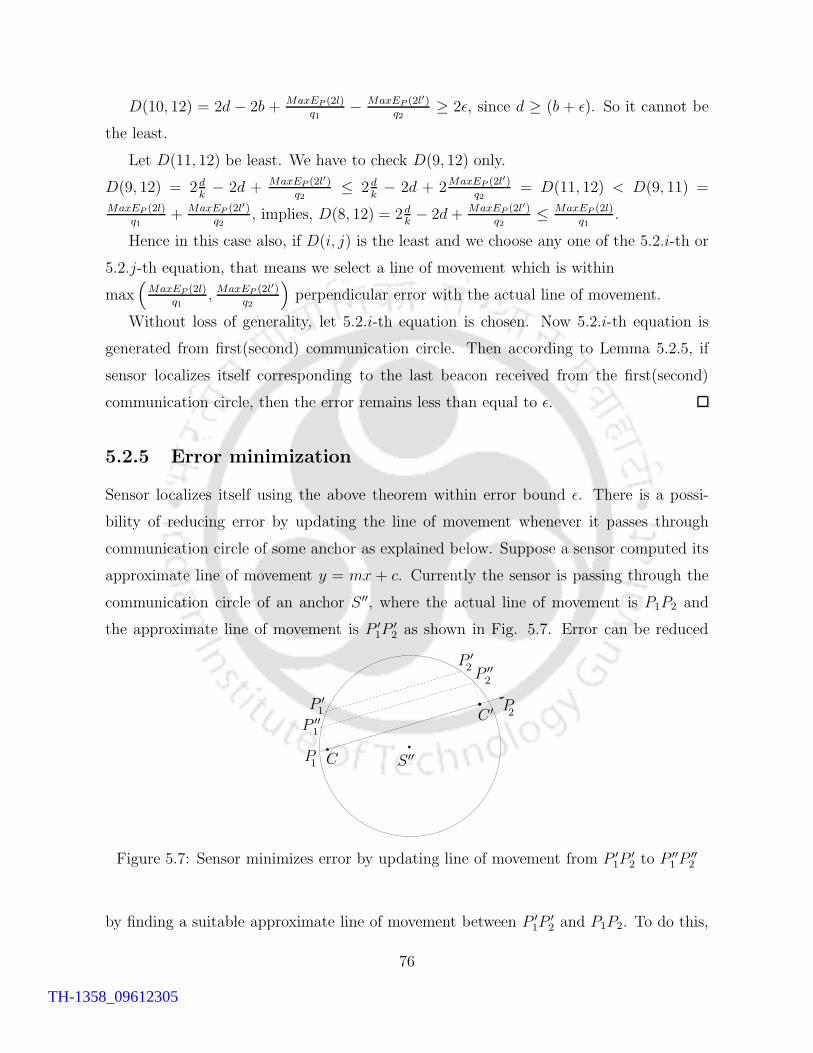
D(10, 12) = 2d − 2b + MaxEP (2l)q1
− MaxEP (2l′)q2
≥ 2ε, since d ≥ (b + ε). So it cannot be
the least.
Let D(11, 12) be least. We have to check D(9, 12) only.
D(9, 12) = 2 dk− 2d + MaxEP (2l′)
q2≤ 2 d
k− 2d + 2MaxEP (2l′)
q2= D(11, 12) < D(9, 11) =
MaxEP (2l)q1
+ MaxEP (2l′)q2
, implies, D(8, 12) = 2 dk− 2d+ MaxEP (2l′)
q2≤ MaxEP (2l)
q1.
Hence in this case also, if D(i, j) is the least and we choose any one of the 5.2.i-th or
5.2.j-th equation, that means we select a line of movement which is within
max(
MaxEP (2l)q1
, MaxEP (2l′)q2
)
perpendicular error with the actual line of movement.
Without loss of generality, let 5.2.i-th equation is chosen. Now 5.2.i-th equation is
generated from first(second) communication circle. Then according to Lemma 5.2.5, if
sensor localizes itself corresponding to the last beacon received from the first(second)
communication circle, then the error remains less than equal to ε.
5.2.5 Error minimization
Sensor localizes itself using the above theorem within error bound ε. There is a possi-
bility of reducing error by updating the line of movement whenever it passes through
communication circle of some anchor as explained below. Suppose a sensor computed its
approximate line of movement y = mx + c. Currently the sensor is passing through the
communication circle of an anchor S ′′, where the actual line of movement is P1P2 and
the approximate line of movement is P ′1P
′2 as shown in Fig. 5.7. Error can be reduced
P
P
P ′
P ′
P ′′
P ′′
S ′′C
C ′1
1
1
2
22
Figure 5.7: Sensor minimizes error by updating line of movement from P ′1P
′2 to P ′′
1 P′′2
by finding a suitable approximate line of movement between P ′1P
′2 and P1P2. To do this,
76
TH-1358_09612305
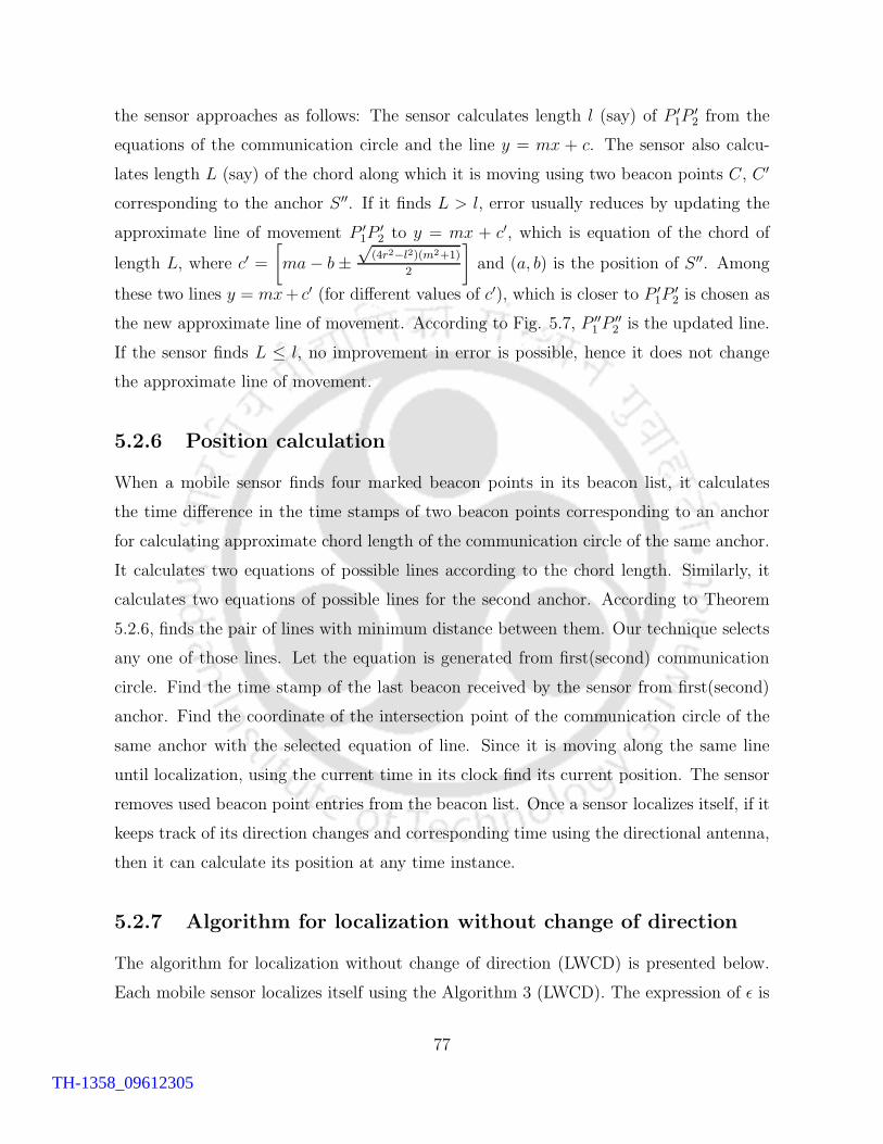
the sensor approaches as follows: The sensor calculates length l (say) of P ′1P
′2 from the
equations of the communication circle and the line y = mx + c. The sensor also calcu-
lates length L (say) of the chord along which it is moving using two beacon points C, C ′
corresponding to the anchor S ′′. If it finds L > l, error usually reduces by updating the
approximate line of movement P ′1P
′2 to y = mx + c′, which is equation of the chord of
length L, where c′ =
[
ma− b±√
(4r2−l2)(m2+1)
2
]
and (a, b) is the position of S ′′. Among
these two lines y = mx+ c′ (for different values of c′), which is closer to P ′1P
′2 is chosen as
the new approximate line of movement. According to Fig. 5.7, P ′′1 P
′′2 is the updated line.
If the sensor finds L ≤ l, no improvement in error is possible, hence it does not change
the approximate line of movement.
5.2.6 Position calculation
When a mobile sensor finds four marked beacon points in its beacon list, it calculates
the time difference in the time stamps of two beacon points corresponding to an anchor
for calculating approximate chord length of the communication circle of the same anchor.
It calculates two equations of possible lines according to the chord length. Similarly, it
calculates two equations of possible lines for the second anchor. According to Theorem
5.2.6, finds the pair of lines with minimum distance between them. Our technique selects
any one of those lines. Let the equation is generated from first(second) communication
circle. Find the time stamp of the last beacon received by the sensor from first(second)
anchor. Find the coordinate of the intersection point of the communication circle of the
same anchor with the selected equation of line. Since it is moving along the same line
until localization, using the current time in its clock find its current position. The sensor
removes used beacon point entries from the beacon list. Once a sensor localizes itself, if it
keeps track of its direction changes and corresponding time using the directional antenna,
then it can calculate its position at any time instance.
5.2.7 Algorithm for localization without change of direction
The algorithm for localization without change of direction (LWCD) is presented below.
Each mobile sensor localizes itself using the Algorithm 3 (LWCD). The expression of ε is
77
TH-1358_09612305
chosen for the algorithm depending on the presence of radio propagation irregularity as
described in section 5.2.4.
Algorithm 3 LWCD
1: Mobile sensor begins localization process by moving with a uniform velocity until localiza-tion.
2: Maintains beacon list as described in section 5.2.2.3: if there are four marked beacon points in beacon list such that the distance between the lines,
which are passing through the anchors parallel to the direction of the sensor’s movement isat least ε then
4: The sensor calculates the current position according to section 5.2.6.5: end if
5.3 Localization without Change of Direction in Pres-
ence of Obstacles
In this section we localize mobile sensors in presence of obstacles. By obstacles, we mean
anything which are blocking the beacons from reaching to the sensor. In this method,
the perpendicular error remains same with LWCD, i.e., maximum perpendicular error on
any calculated chord length 2l is MaxEP (2l). Beacons are obstructed by the obstacles
as shown in Fig. 5.8. Here, the actual line of movement is P1P2, whereas P ′1P
′2 is the
calculated chord length corresponding to the beacon points. In presence of obstacles,
there are two possible cases which effect localization as mentioned below. In case 1, the
sensor receives at least two beacons including the first and last beacons but the remaining
beacons are blocked by the obstacles. Here the problem is, whenever beacons are blocked
after receiving at least the first beacon c1, sensor marks the beacon c2 as the last beacon
point for the communication circle as the waiting time t0 (Ref. section 5.2.2) exceeds
before receiving next beacon c3. So last beacon point is selected wrongly. Hence the
actual last beacon c4 is received but is not marked as beacon point as shown in Fig. 5.8a.
We can avoid this problem by increasing the waiting time t0 of the sensor to t2r, where
t2r is defined as the time required for a sensor to travel 2r distance. Since 2r is the length
of the diameter of the communication circle, by setting the waiting time equal to t2r, a
sensor always detects the actual last beacon in case 1. So, according to Fig. 5.8a, now
78
TH-1358_09612305
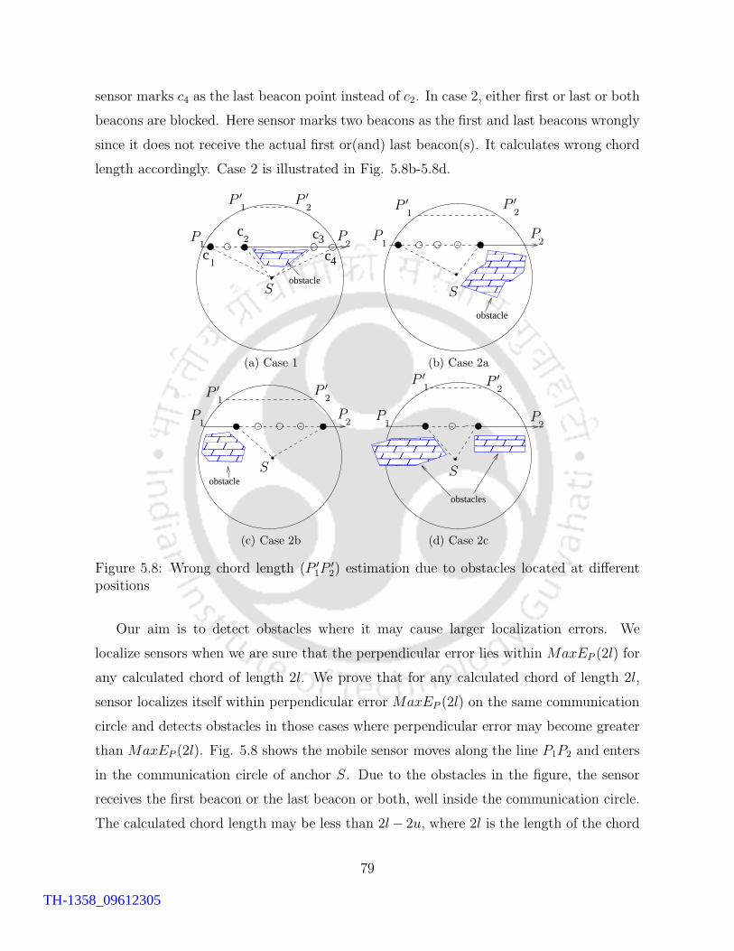
sensor marks c4 as the last beacon point instead of c2. In case 2, either first or last or both
beacons are blocked. Here sensor marks two beacons as the first and last beacons wrongly
since it does not receive the actual first or(and) last beacon(s). It calculates wrong chord
length accordingly. Case 2 is illustrated in Fig. 5.8b-5.8d.
obstacle
c
c3
c4
cP P
P ′ P ′
S
1
1
12
2
2
(a) Case 1
obstacle
P P
P ′P ′
S
1
1
2
2
(b) Case 2a
obstacle
PP
P ′ P ′
S
1
1
2
2
(c) Case 2b
obstacles
P P
P ′P ′
S
1
1
2
2
(d) Case 2c
Figure 5.8: Wrong chord length (P ′1P
′2) estimation due to obstacles located at different
positions
Our aim is to detect obstacles where it may cause larger localization errors. We
localize sensors when we are sure that the perpendicular error lies within MaxEP (2l) for
any calculated chord of length 2l. We prove that for any calculated chord of length 2l,
sensor localizes itself within perpendicular error MaxEP (2l) on the same communication
circle and detects obstacles in those cases where perpendicular error may become greater
than MaxEP (2l). Fig. 5.8 shows the mobile sensor moves along the line P1P2 and enters
in the communication circle of anchor S. Due to the obstacles in the figure, the sensor
receives the first beacon or the last beacon or both, well inside the communication circle.
The calculated chord length may be less than 2l− 2u, where 2l is the length of the chord
79
TH-1358_09612305
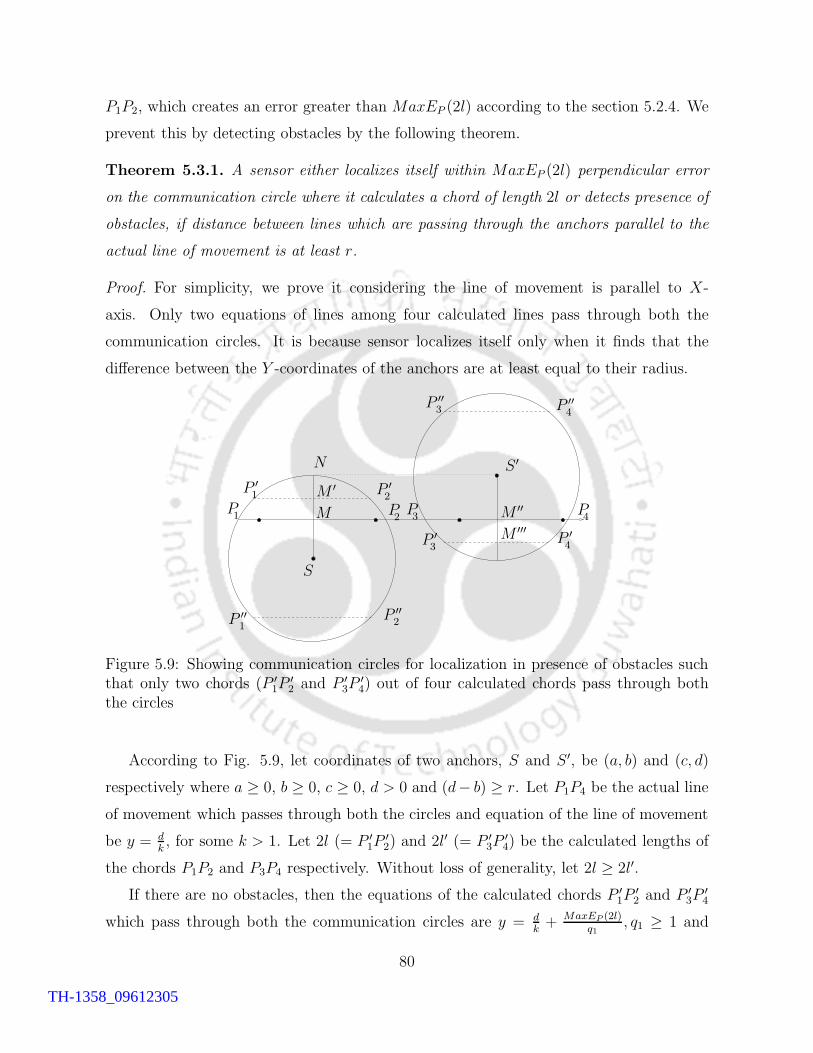
P1P2, which creates an error greater than MaxEP (2l) according to the section 5.2.4. We
prevent this by detecting obstacles by the following theorem.
Theorem 5.3.1. A sensor either localizes itself within MaxEP (2l) perpendicular error
on the communication circle where it calculates a chord of length 2l or detects presence of
obstacles, if distance between lines which are passing through the anchors parallel to the
actual line of movement is at least r.
Proof. For simplicity, we prove it considering the line of movement is parallel to X-
axis. Only two equations of lines among four calculated lines pass through both the
communication circles. It is because sensor localizes itself only when it finds that the
difference between the Y -coordinates of the anchors are at least equal to their radius.
1
1
1
2
2
2
3
3
3
4
4
4
M
M ′
M ′′
M ′′′
S
S ′
P PPPP ′
P ′P ′
P ′
P ′′P ′′
P ′′P ′′
N
Figure 5.9: Showing communication circles for localization in presence of obstacles suchthat only two chords (P ′
1P′2 and P ′
3P′4) out of four calculated chords pass through both
the circles
According to Fig. 5.9, let coordinates of two anchors, S and S ′, be (a, b) and (c, d)
respectively where a ≥ 0, b ≥ 0, c ≥ 0, d > 0 and (d− b) ≥ r. Let P1P4 be the actual line
of movement which passes through both the circles and equation of the line of movement
be y = dk, for some k > 1. Let 2l (= P ′
1P′2) and 2l′ (= P ′
3P′4) be the calculated lengths of
the chords P1P2 and P3P4 respectively. Without loss of generality, let 2l ≥ 2l′.
If there are no obstacles, then the equations of the calculated chords P ′1P
′2 and P ′
3P′4
which pass through both the communication circles are y = dk+ MaxEP (2l)
q1, q1 ≥ 1 and
80
TH-1358_09612305
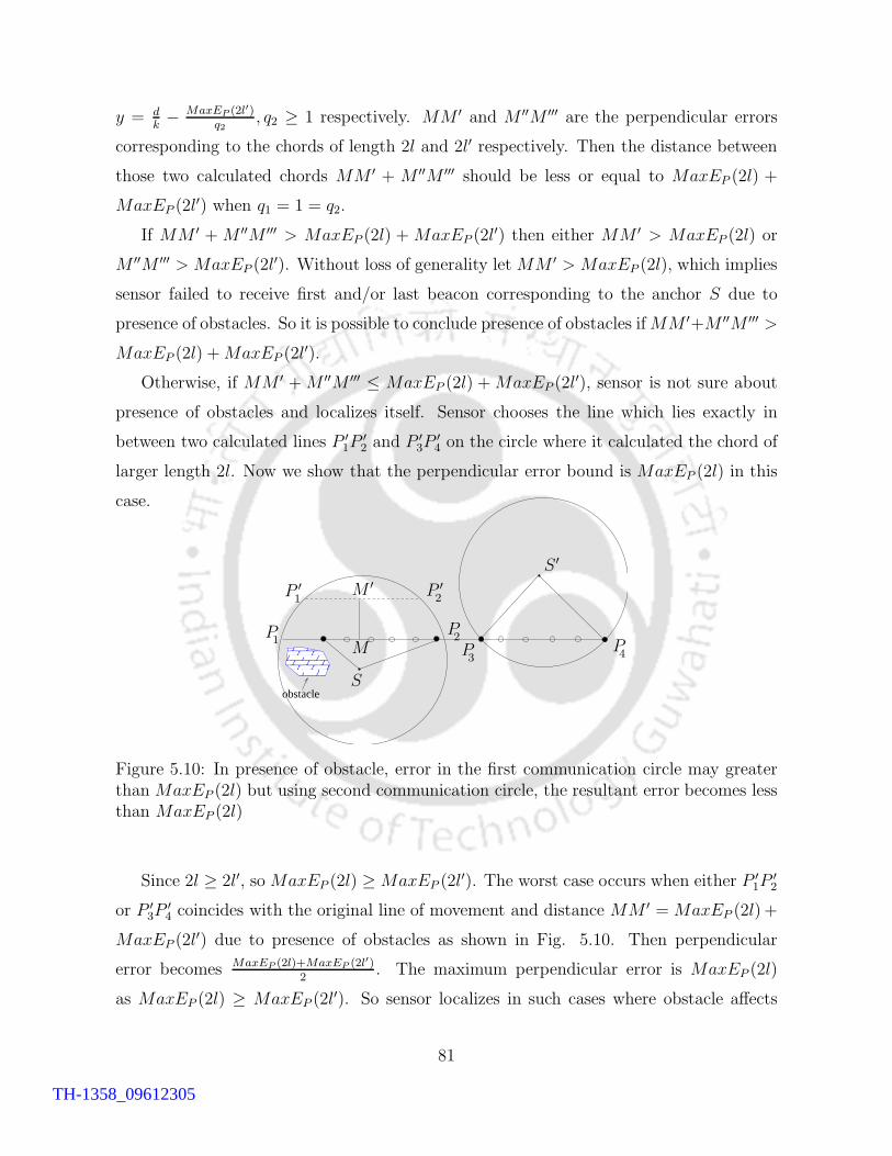
y = dk− MaxEP (2l′)
q2, q2 ≥ 1 respectively. MM ′ and M ′′M ′′′ are the perpendicular errors
corresponding to the chords of length 2l and 2l′ respectively. Then the distance between
those two calculated chords MM ′ + M ′′M ′′′ should be less or equal to MaxEP (2l) +
MaxEP (2l′) when q1 = 1 = q2.
If MM ′ + M ′′M ′′′ > MaxEP (2l) + MaxEP (2l′) then either MM ′ > MaxEP (2l) or
M ′′M ′′′ > MaxEP (2l′). Without loss of generality let MM ′ > MaxEP (2l), which implies
sensor failed to receive first and/or last beacon corresponding to the anchor S due to
presence of obstacles. So it is possible to conclude presence of obstacles ifMM ′+M ′′M ′′′ >
MaxEP (2l) +MaxEP (2l′).
Otherwise, if MM ′ +M ′′M ′′′ ≤ MaxEP (2l) +MaxEP (2l′), sensor is not sure about
presence of obstacles and localizes itself. Sensor chooses the line which lies exactly in
between two calculated lines P ′1P
′2 and P ′
3P′4 on the circle where it calculated the chord of
larger length 2l. Now we show that the perpendicular error bound is MaxEP (2l) in this
case.
obstacle
1
1
2
2
3 4M
M ′
S
S ′
PPPP
P ′ P ′
Figure 5.10: In presence of obstacle, error in the first communication circle may greaterthan MaxEP (2l) but using second communication circle, the resultant error becomes lessthan MaxEP (2l)
Since 2l ≥ 2l′, so MaxEP (2l) ≥ MaxEP (2l′). The worst case occurs when either P ′
1P′2
or P ′3P
′4 coincides with the original line of movement and distance MM ′ = MaxEP (2l) +
MaxEP (2l′) due to presence of obstacles as shown in Fig. 5.10. Then perpendicular
error becomes MaxEP (2l)+MaxEP (2l′)2
. The maximum perpendicular error is MaxEP (2l)
as MaxEP (2l) ≥ MaxEP (2l′). So sensor localizes in such cases where obstacle affects
81
TH-1358_09612305
localization but the perpendicular error remains within its bound.
In presence of obstacles, percentage of localization is an important factor along with
localization error. For better localization percentage, we can relax the condition from
MM ′ + M ′′M ′′′ ≤ MaxEP (2l) + MaxEP (2l′) to MM ′ + M ′′M ′′′ ≤ 2(MaxEP (2l) +
MaxEP (2l′)) for doing localization. Then perpendicular error increases accordingly and
perpendicular error bound becomes 2MaxEP (2l). Section 5.4 shows average errors for
both these cases.
5.3.1 Position calculation in presence of obstacles
Sensor calculates two lines which pass through both the communication circles using the
calculated chord lengths 2l, 2l′, say, from the communication circles of the anchors as
explained above. If distance between these two lines is less than equal to MaxEP (2l) +
MaxEP (2l′), it chooses the line lies exactly in between of those two lines and on the
communication circle on which it calculated the chord with greater length. Then it
localizes itself using the elapsed time between the current time and time stamp of the
last beacon received from that anchor. Otherwise sensor avoids localization detecting
obstacles and looks for beacons from other anchors for localization.
5.3.2 Algorithm in presence of obstacles
The algorithm for localization without change of direction in presence of obstacles (LWCDPO)
is given below. Each sensor localizes itself using the proposed Algorithm 4 (LWCDPO)
in presence of obstacles.
Algorithm 4 LWCDPO
1: Mobile sensor does not change its direction of movement during localization.2: Maintains beacon list as described in section 5.2.2 with waiting time t2r.3: if there are at least four marked beacon points in beacon list such that the distance between
the lines, which are passing through the anchors parallel to the actual line of movement isat least r then
4: Sensor either detects obstacles or calculates the current position according to Theorem5.3.1.
5: end if
82
TH-1358_09612305
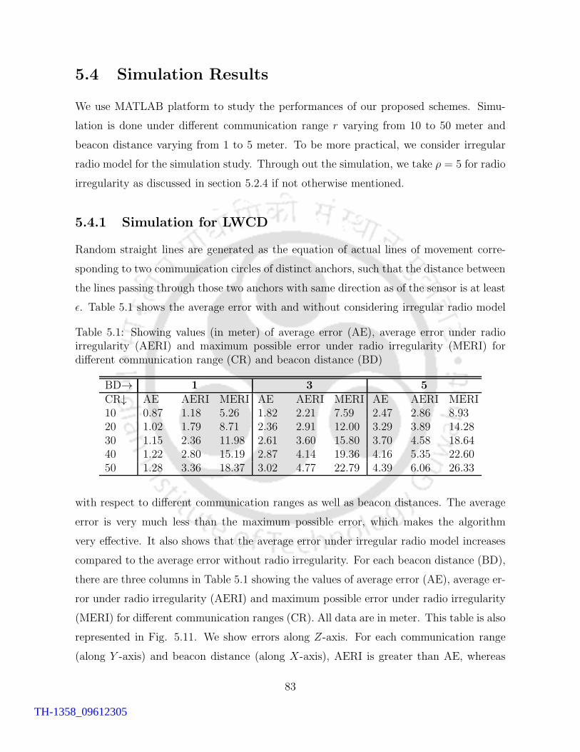
5.4 Simulation Results
We use MATLAB platform to study the performances of our proposed schemes. Simu-
lation is done under different communication range r varying from 10 to 50 meter and
beacon distance varying from 1 to 5 meter. To be more practical, we consider irregular
radio model for the simulation study. Through out the simulation, we take ρ = 5 for radio
irregularity as discussed in section 5.2.4 if not otherwise mentioned.
5.4.1 Simulation for LWCD
Random straight lines are generated as the equation of actual lines of movement corre-
sponding to two communication circles of distinct anchors, such that the distance between
the lines passing through those two anchors with same direction as of the sensor is at least
ε. Table 5.1 shows the average error with and without considering irregular radio model
Table 5.1: Showing values (in meter) of average error (AE), average error under radioirregularity (AERI) and maximum possible error under radio irregularity (MERI) fordifferent communication range (CR) and beacon distance (BD)
BD→ 1 3 5CR↓ AE AERI MERI AE AERI MERI AE AERI MERI10 0.87 1.18 5.26 1.82 2.21 7.59 2.47 2.86 8.9320 1.02 1.79 8.71 2.36 2.91 12.00 3.29 3.89 14.2830 1.15 2.36 11.98 2.61 3.60 15.80 3.70 4.58 18.6440 1.22 2.80 15.19 2.87 4.14 19.36 4.16 5.35 22.6050 1.28 3.36 18.37 3.02 4.77 22.79 4.39 6.06 26.33
with respect to different communication ranges as well as beacon distances. The average
error is very much less than the maximum possible error, which makes the algorithm
very effective. It also shows that the average error under irregular radio model increases
compared to the average error without radio irregularity. For each beacon distance (BD),
there are three columns in Table 5.1 showing the values of average error (AE), average er-
ror under radio irregularity (AERI) and maximum possible error under radio irregularity
(MERI) for different communication ranges (CR). All data are in meter. This table is also
represented in Fig. 5.11. We show errors along Z-axis. For each communication range
(along Y -axis) and beacon distance (along X-axis), AERI is greater than AE, whereas
83
TH-1358_09612305
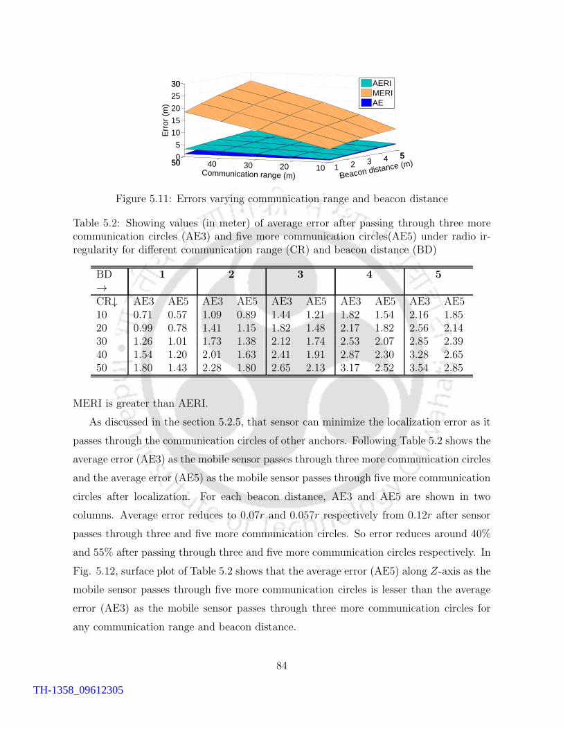
1 2 3 4 55
1020304050500
5
10
15
20
25
3030
Beacon distance (m)Communication range (m)
E
rror
(m
)
AERIMERIAE
Figure 5.11: Errors varying communication range and beacon distance
Table 5.2: Showing values (in meter) of average error after passing through three morecommunication circles (AE3) and five more communication circles(AE5) under radio ir-regularity for different communication range (CR) and beacon distance (BD)
BD→
1 2 3 4 5
CR↓ AE3 AE5 AE3 AE5 AE3 AE5 AE3 AE5 AE3 AE510 0.71 0.57 1.09 0.89 1.44 1.21 1.82 1.54 2.16 1.8520 0.99 0.78 1.41 1.15 1.82 1.48 2.17 1.82 2.56 2.1430 1.26 1.01 1.73 1.38 2.12 1.74 2.53 2.07 2.85 2.3940 1.54 1.20 2.01 1.63 2.41 1.91 2.87 2.30 3.28 2.6550 1.80 1.43 2.28 1.80 2.65 2.13 3.17 2.52 3.54 2.85
MERI is greater than AERI.
As discussed in the section 5.2.5, that sensor can minimize the localization error as it
passes through the communication circles of other anchors. Following Table 5.2 shows the
average error (AE3) as the mobile sensor passes through three more communication circles
and the average error (AE5) as the mobile sensor passes through five more communication
circles after localization. For each beacon distance, AE3 and AE5 are shown in two
columns. Average error reduces to 0.07r and 0.057r respectively from 0.12r after sensor
passes through three and five more communication circles. So error reduces around 40%
and 55% after passing through three and five more communication circles respectively. In
Fig. 5.12, surface plot of Table 5.2 shows that the average error (AE5) along Z-axis as the
mobile sensor passes through five more communication circles is lesser than the average
error (AE3) as the mobile sensor passes through three more communication circles for
any communication range and beacon distance.
84
TH-1358_09612305
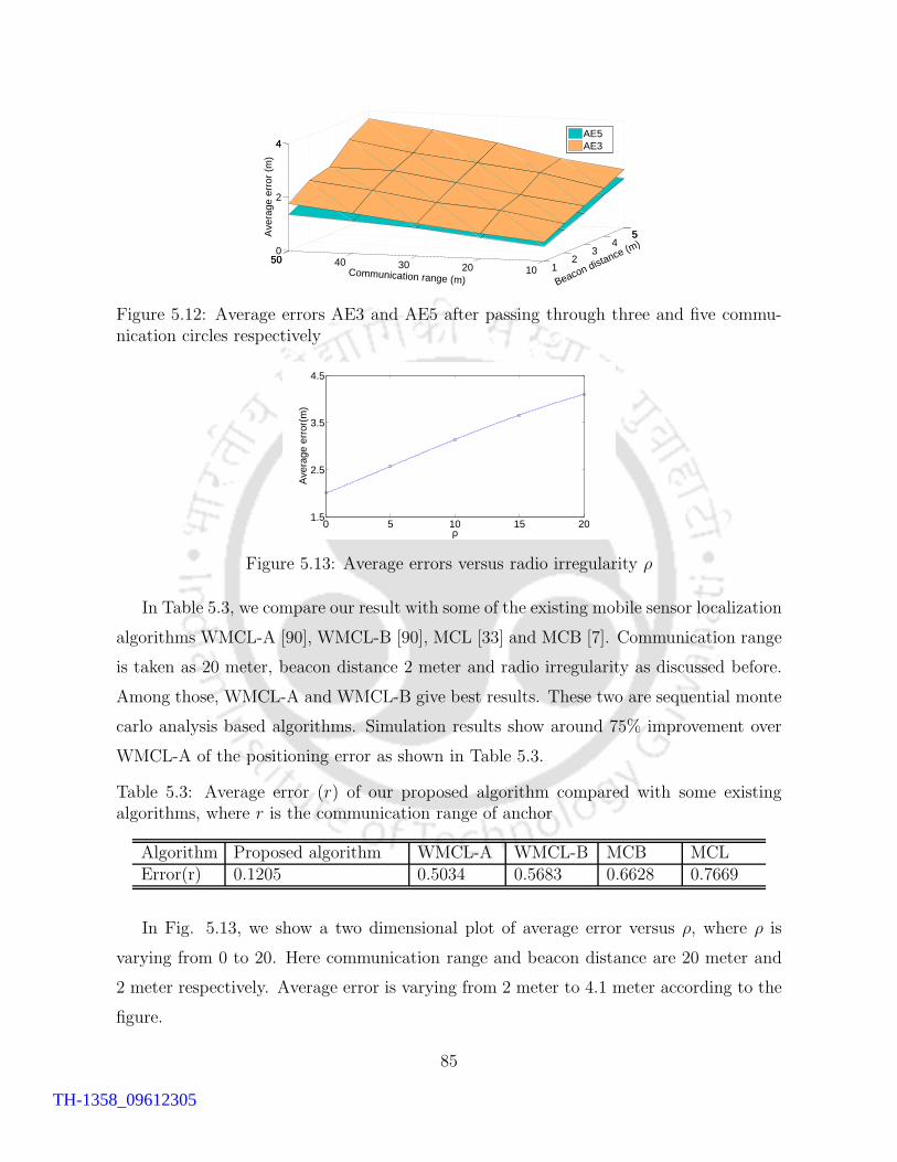
12
34
55
1020304050500
2
44
Beacon distance (m)
Communication range (m)
Ave
rage
err
or (
m)
AE5AE3
Figure 5.12: Average errors AE3 and AE5 after passing through three and five commu-nication circles respectively
0 5 10 15 201.5
2.5
3.5
4.5
ρ
Ave
rage
err
or(m
)
Figure 5.13: Average errors versus radio irregularity ρ
In Table 5.3, we compare our result with some of the existing mobile sensor localization
algorithms WMCL-A [90], WMCL-B [90], MCL [33] and MCB [7]. Communication range
is taken as 20 meter, beacon distance 2 meter and radio irregularity as discussed before.
Among those, WMCL-A and WMCL-B give best results. These two are sequential monte
carlo analysis based algorithms. Simulation results show around 75% improvement over
WMCL-A of the positioning error as shown in Table 5.3.
Table 5.3: Average error (r) of our proposed algorithm compared with some existingalgorithms, where r is the communication range of anchor
Algorithm Proposed algorithm WMCL-A WMCL-B MCB MCLError(r) 0.1205 0.5034 0.5683 0.6628 0.7669
In Fig. 5.13, we show a two dimensional plot of average error versus ρ, where ρ is
varying from 0 to 20. Here communication range and beacon distance are 20 meter and
2 meter respectively. Average error is varying from 2 meter to 4.1 meter according to the
figure.
85
TH-1358_09612305
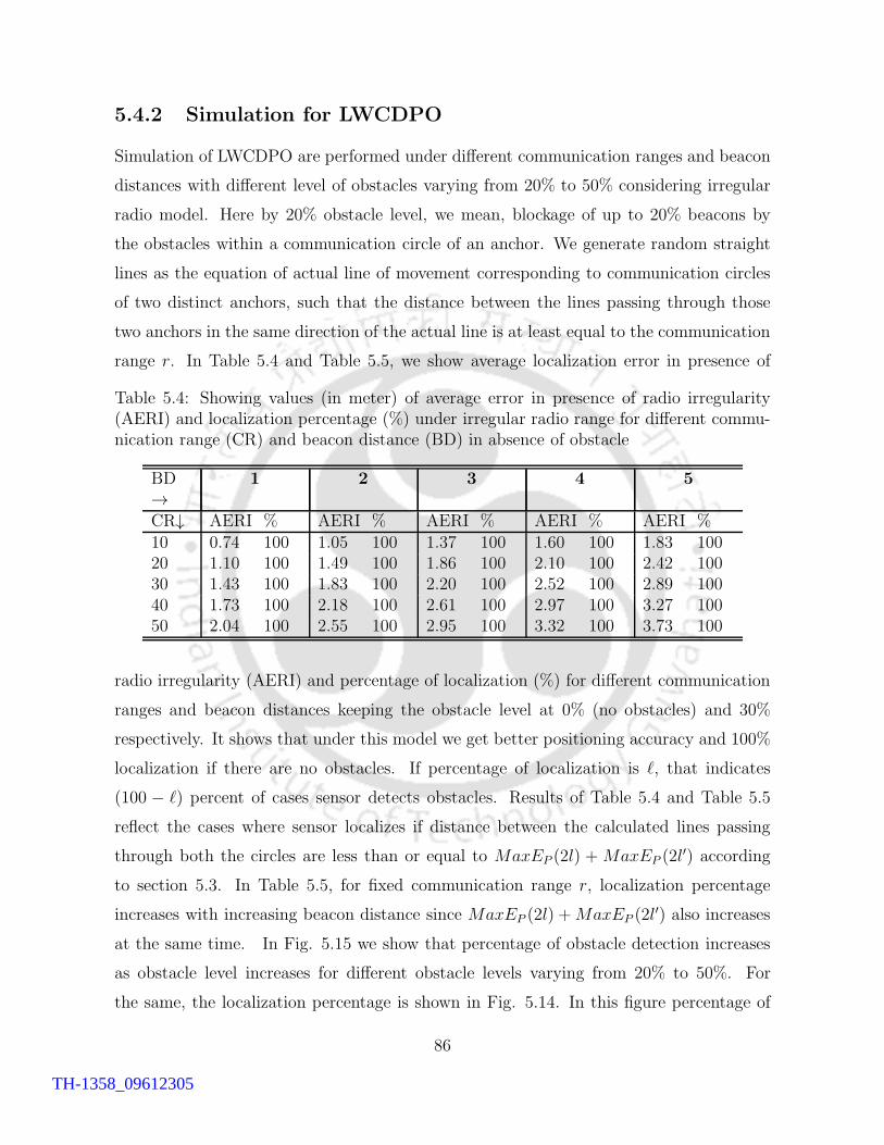
5.4.2 Simulation for LWCDPO
Simulation of LWCDPO are performed under different communication ranges and beacon
distances with different level of obstacles varying from 20% to 50% considering irregular
radio model. Here by 20% obstacle level, we mean, blockage of up to 20% beacons by
the obstacles within a communication circle of an anchor. We generate random straight
lines as the equation of actual line of movement corresponding to communication circles
of two distinct anchors, such that the distance between the lines passing through those
two anchors in the same direction of the actual line is at least equal to the communication
range r. In Table 5.4 and Table 5.5, we show average localization error in presence of
Table 5.4: Showing values (in meter) of average error in presence of radio irregularity(AERI) and localization percentage (%) under irregular radio range for different commu-nication range (CR) and beacon distance (BD) in absence of obstacle
BD→
1 2 3 4 5
CR↓ AERI % AERI % AERI % AERI % AERI %10 0.74 100 1.05 100 1.37 100 1.60 100 1.83 10020 1.10 100 1.49 100 1.86 100 2.10 100 2.42 10030 1.43 100 1.83 100 2.20 100 2.52 100 2.89 10040 1.73 100 2.18 100 2.61 100 2.97 100 3.27 10050 2.04 100 2.55 100 2.95 100 3.32 100 3.73 100
radio irregularity (AERI) and percentage of localization (%) for different communication
ranges and beacon distances keeping the obstacle level at 0% (no obstacles) and 30%
respectively. It shows that under this model we get better positioning accuracy and 100%
localization if there are no obstacles. If percentage of localization is `, that indicates
(100 − `) percent of cases sensor detects obstacles. Results of Table 5.4 and Table 5.5
reflect the cases where sensor localizes if distance between the calculated lines passing
through both the circles are less than or equal to MaxEP (2l) + MaxEP (2l′) according
to section 5.3. In Table 5.5, for fixed communication range r, localization percentage
increases with increasing beacon distance since MaxEP (2l) +MaxEP (2l′) also increases
at the same time. In Fig. 5.15 we show that percentage of obstacle detection increases
as obstacle level increases for different obstacle levels varying from 20% to 50%. For
the same, the localization percentage is shown in Fig. 5.14. In this figure percentage of
86
TH-1358_09612305
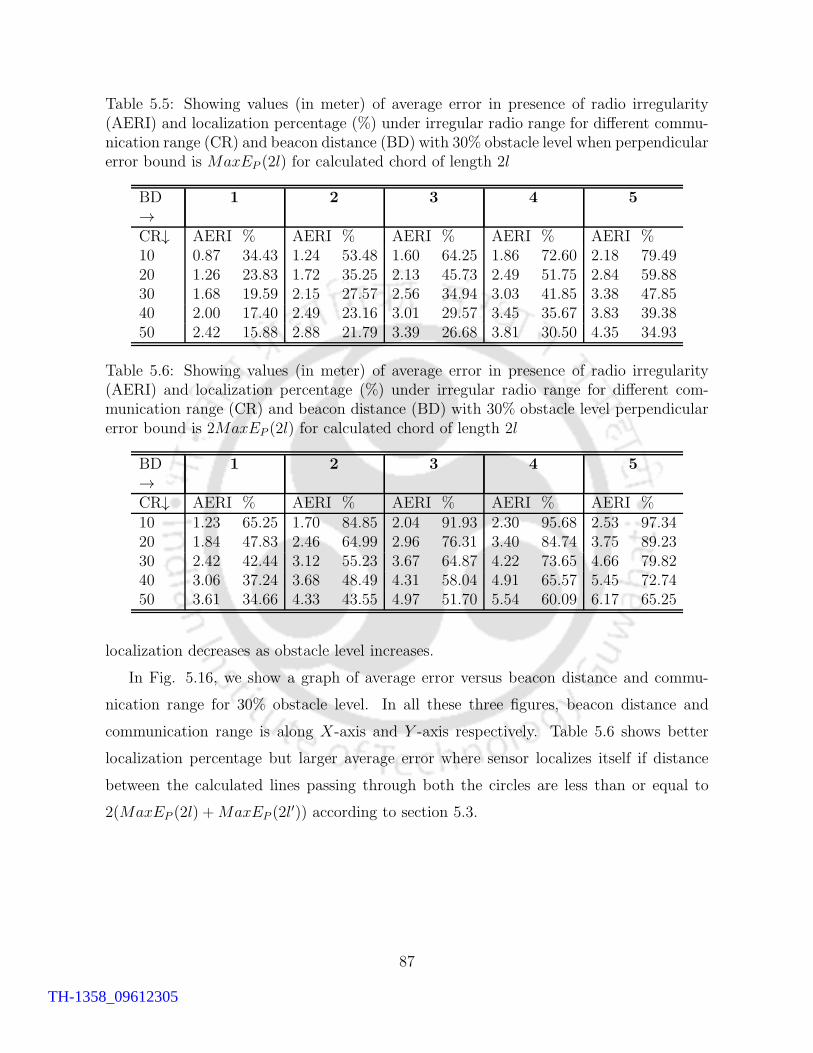
Table 5.5: Showing values (in meter) of average error in presence of radio irregularity(AERI) and localization percentage (%) under irregular radio range for different commu-nication range (CR) and beacon distance (BD) with 30% obstacle level when perpendicularerror bound is MaxEP (2l) for calculated chord of length 2l
BD→
1 2 3 4 5
CR↓ AERI % AERI % AERI % AERI % AERI %10 0.87 34.43 1.24 53.48 1.60 64.25 1.86 72.60 2.18 79.4920 1.26 23.83 1.72 35.25 2.13 45.73 2.49 51.75 2.84 59.8830 1.68 19.59 2.15 27.57 2.56 34.94 3.03 41.85 3.38 47.8540 2.00 17.40 2.49 23.16 3.01 29.57 3.45 35.67 3.83 39.3850 2.42 15.88 2.88 21.79 3.39 26.68 3.81 30.50 4.35 34.93
Table 5.6: Showing values (in meter) of average error in presence of radio irregularity(AERI) and localization percentage (%) under irregular radio range for different com-munication range (CR) and beacon distance (BD) with 30% obstacle level perpendicularerror bound is 2MaxEP (2l) for calculated chord of length 2l
BD→
1 2 3 4 5
CR↓ AERI % AERI % AERI % AERI % AERI %10 1.23 65.25 1.70 84.85 2.04 91.93 2.30 95.68 2.53 97.3420 1.84 47.83 2.46 64.99 2.96 76.31 3.40 84.74 3.75 89.2330 2.42 42.44 3.12 55.23 3.67 64.87 4.22 73.65 4.66 79.8240 3.06 37.24 3.68 48.49 4.31 58.04 4.91 65.57 5.45 72.7450 3.61 34.66 4.33 43.55 4.97 51.70 5.54 60.09 6.17 65.25
localization decreases as obstacle level increases.
In Fig. 5.16, we show a graph of average error versus beacon distance and commu-
nication range for 30% obstacle level. In all these three figures, beacon distance and
communication range is along X-axis and Y -axis respectively. Table 5.6 shows better
localization percentage but larger average error where sensor localizes itself if distance
between the calculated lines passing through both the circles are less than or equal to
2(MaxEP (2l) +MaxEP (2l′)) according to section 5.3.
87
TH-1358_09612305
12
34
55
1020
3040
5050500
20
40
60
80
100100
Beacon distance (m)Communication range (m)
Per
cent
age
of lo
caliz
atio
n (%
)
(a) 20% obstacle level
12
34
555
1020
3040
5050500
20
40
60
80
100100
Beacon distance (m)Communication range (m)
Per
cent
age
of lo
caliz
atio
n (%
)
(b) 30% obstacle level
12
34
55
1020
3040
5050500
20
40
60
80
100100
Beacon distance (m)Communication range (m)
Per
cent
age
of lo
caliz
atio
n (%
)
(c) 40% obstacle level
12
34
55
1020
3040
50500
20
40
60
80
100100
Beacon distance (m)Communication range (m)P
erce
ntag
e of
loca
lizat
ion
(%)
(d) 50% obstacle level
Figure 5.14: Percentage of localization decreases as obstacle level increases
12
34
55
1020
3040
50500
20
40
60
80
100100
Beacon distance (m)Communication range (m)
Obs
tacl
e de
tect
ion
(%)
(a) 20% obstacle level
12
34
55
1020
3040
50500
20
40
60
80
100100
Beacon distance (m)Communication range (m)
Obs
tacl
e de
tect
ion
(%)
(b) 30% obstacle level
12
34
55
1020
3040
50500
20
40
60
80
100100
Beacon distance (m)Communication range (m)
Obs
tacl
e de
tect
ion
(%)
(c) 40% obstacle level
12
34
55
1020
3040
50500
20
40
60
80
100100
Beacon distance (m)Communication range (m)
Obs
tacl
e de
tect
ion
(%)
(d) 50% obstacle level
Figure 5.15: Obstacle detection increases as obstacle level increases
88
TH-1358_09612305
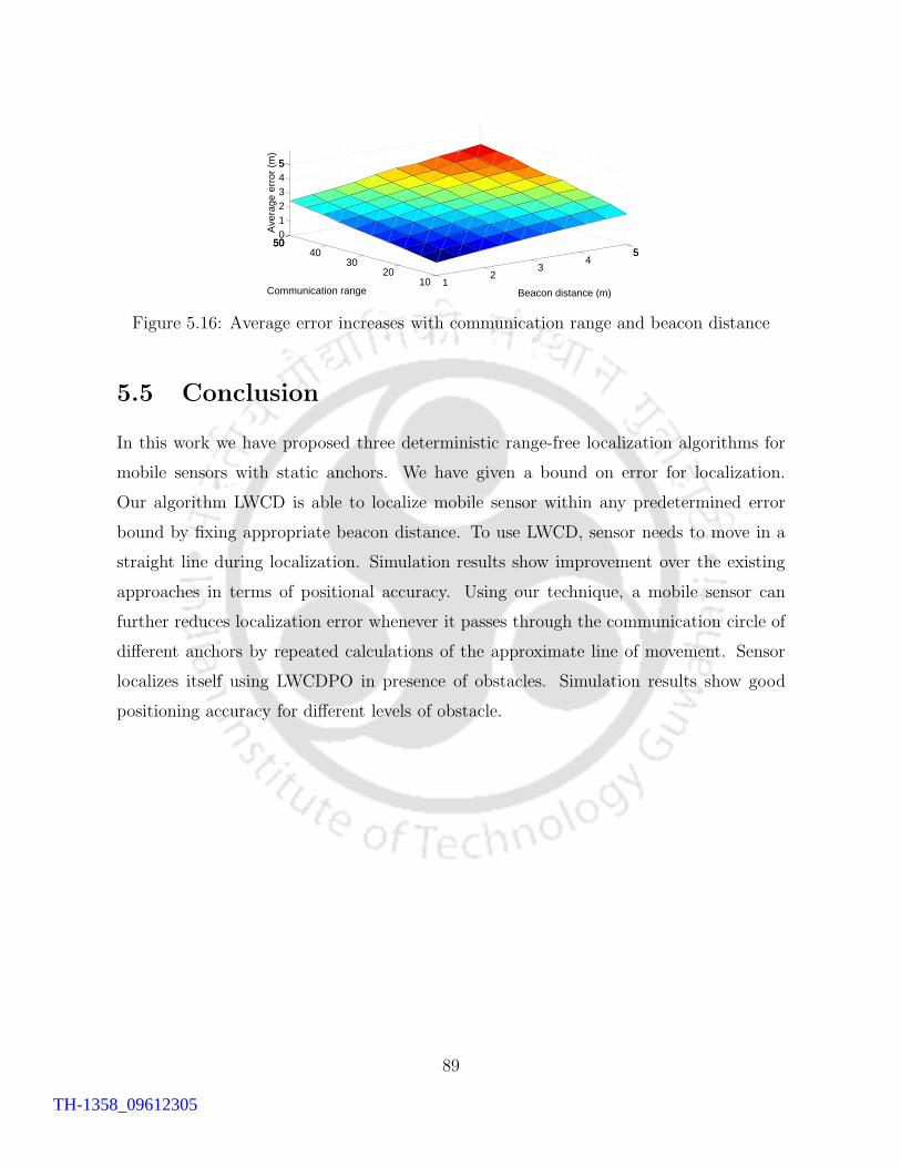
12
34
55
1020
3040
5050500123455
Beacon distance (m)Communication range
Ave
rage
err
or (
m)
Figure 5.16: Average error increases with communication range and beacon distance
5.5 Conclusion
In this work we have proposed three deterministic range-free localization algorithms for
mobile sensors with static anchors. We have given a bound on error for localization.
Our algorithm LWCD is able to localize mobile sensor within any predetermined error
bound by fixing appropriate beacon distance. To use LWCD, sensor needs to move in a
straight line during localization. Simulation results show improvement over the existing
approaches in terms of positional accuracy. Using our technique, a mobile sensor can
further reduces localization error whenever it passes through the communication circle of
different anchors by repeated calculations of the approximate line of movement. Sensor
localizes itself using LWCDPO in presence of obstacles. Simulation results show good
positioning accuracy for different levels of obstacle.
89
TH-1358_09612305

TH-1358_09612305
Chapter 6
Mobile Sensor Localization in
Presence of Obstacles
6.1 Introduction
In the previous chapter, localization of mobile sensors is done assuming sensors do not
change direction during localization. Practically, sensors may need to change direction
within a communication circle depending on the requirements of the underlying applica-
tions. In this chapter we allow change of direction of mobile sensors during localization
and propose the algorithm LCD. LCD localizes a sensor within the communication circle
of one static anchor based on polygonal structures generated by direction changes of mo-
bile sensor. Then we consider the problem where obstacles may present anywhere in the
network and propose another algorithm LPO to localize sensors.
6.1.1 Our contribution
The algorithm LCD localizes mobile sensors which change direction during localization.
Simulation results show 67% and 63% improvement of the positioning error over the ex-
isting algorithm [90] corresponding to two different selection criteria. We propose another
algorithm LPO which localizes sensors in presence of obstacles with change of direction.
It achieves 52% and 49% improvements corresponding to two different selection criteria
in terms of localization accuracy compared to existing works.
91
TH-1358_09612305
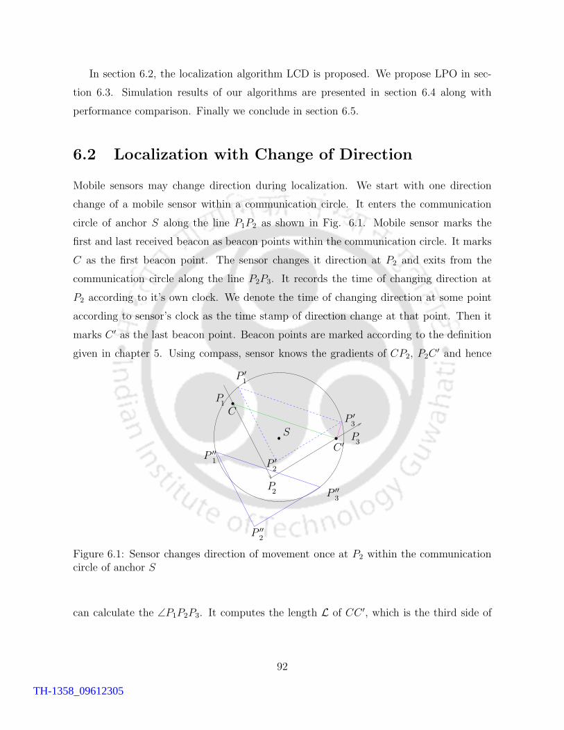
In section 6.2, the localization algorithm LCD is proposed. We propose LPO in sec-
tion 6.3. Simulation results of our algorithms are presented in section 6.4 along with
performance comparison. Finally we conclude in section 6.5.
6.2 Localization with Change of Direction
Mobile sensors may change direction during localization. We start with one direction
change of a mobile sensor within a communication circle. It enters the communication
circle of anchor S along the line P1P2 as shown in Fig. 6.1. Mobile sensor marks the
first and last received beacon as beacon points within the communication circle. It marks
C as the first beacon point. The sensor changes it direction at P2 and exits from the
communication circle along the line P2P3. It records the time of changing direction at
P2 according to it’s own clock. We denote the time of changing direction at some point
according to sensor’s clock as the time stamp of direction change at that point. Then it
marks C ′ as the last beacon point. Beacon points are marked according to the definition
given in chapter 5. Using compass, sensor knows the gradients of CP2, P2C′ and hence
P
P
P
P ′
P ′
P ′
P ′′
P ′′
P ′′
S
1
1
1
2
2
2
3
3
3
C
C ′
Figure 6.1: Sensor changes direction of movement once at P2 within the communicationcircle of anchor S
can calculate the ∠P1P2P3. It computes the length L of CC ′, which is the third side of
92
TH-1358_09612305
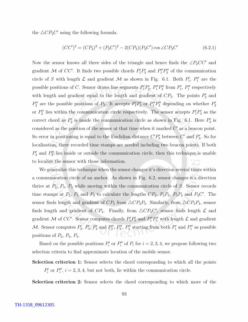
the 4CP2C′ using the following formula.
(CC ′)2 = (CP2)2 + (P2C
′)2 − 2(CP2)(P2C′) cos∠CP2C
′ (6.2.1)
Now the sensor knows all three sides of the triangle and hence finds the ∠P2CC ′ and
gradient M of CC ′. It finds two possible chords P ′1P
′3 and P ′′
1 P′′3 of the communication
circle of S with length L and gradient M as shown in Fig. 6.1. Both P ′1, P
′′1 are the
possible positions of C. Sensor draws line segments P ′1P
′2, P
′′1 P
′′2 from P ′
1, P′′1 respectively
with length and gradient equal to the length and gradient of CP2. The points P ′2 and
P ′′2 are the possible positions of P2. It accepts P ′
1P′3 or P ′′
1 P′′3 depending on whether P ′
2
or P ′′2 lies within the communication circle respectively. The sensor accepts P ′
1P′3 as the
correct chord as P ′2 is inside the communication circle as shown in Fig. 6.1. Here P ′
3 is
considered as the position of the sensor at that time when it marked C ′ as a beacon point.
So error in positioning is equal to the Euclidian distance C ′P ′3 between C ′ and P ′
3. So for
localization, three recorded time stamps are needed including two beacon points. If both
P ′2 and P ′′
2 lies inside or outside the communication circle, then this technique is unable
to localize the sensor with those information.
We generalize this technique when the sensor changes it’s direction several times within
a communication circle of an anchor. As shown in Fig. 6.2, sensor changes it’s direction
thrice at P2, P3, P4 while moving within the communication circle of S. Sensor records
time stamps at P2, P3 and P4 to calculate the lengths CP2, P2P3, P3P4 and P4C′. The
sensor finds length and gradient of CP3 from 4CP2P3. Similarly, from 4CP3P4, sensor
finds length and gradient of CP4. Finally, from 4CP4C′, sensor finds length L and
gradient M of CC ′. Sensor computes chords P ′1P
′5 and P ′′
1 P′′5 with length L and gradient
M. Sensor computes P ′2, P
′3, P
′4 and P ′′
2 , P′′3 , P
′′4 starting from both P ′
1 and P ′′1 as possible
positions of P2, P3, P4.
Based on the possible positions P ′i or P
′′i of Pi for i = 2, 3, 4, we propose following two
selection criteria to find approximate location of the mobile sensor.
Selection criterion 1: Sensor selects the chord corresponding to which all the points
P ′i or P
′′i , i = 2, 3, 4, but not both, lie within the communication circle.
Selection criterion 2: Sensor selects the chord corresponding to which more of the
93
TH-1358_09612305
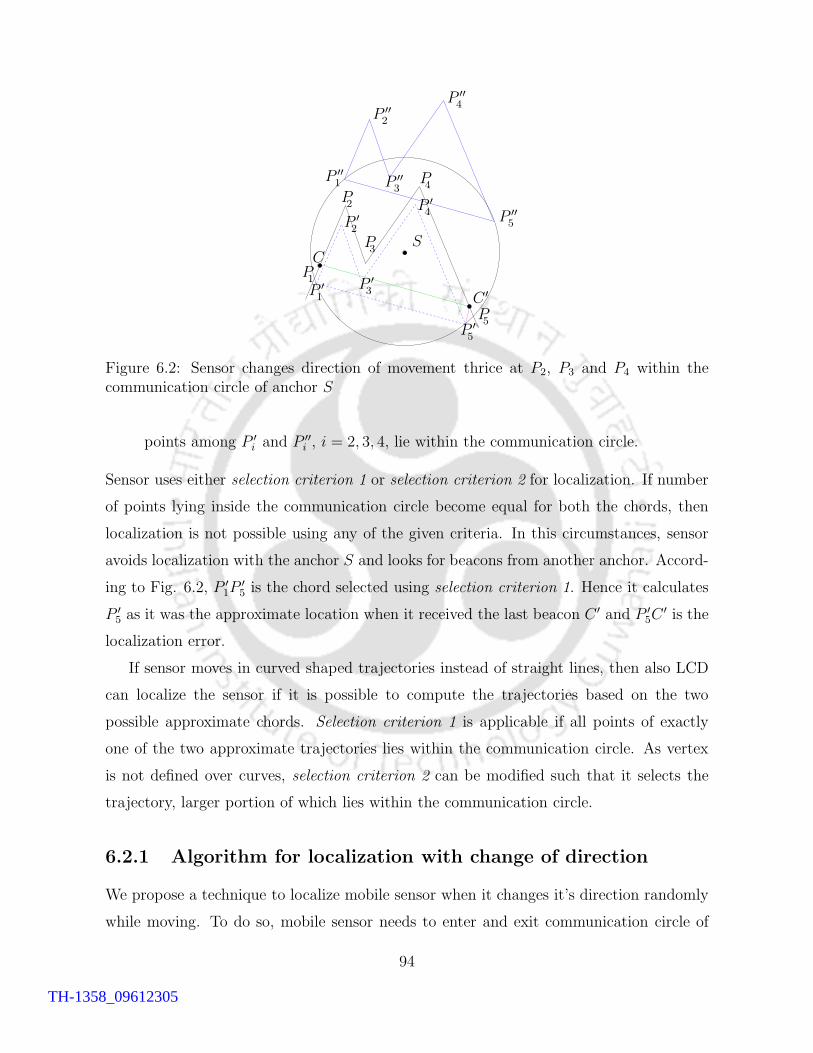
P
P
P
P
P
P ′P ′
P ′P ′
P ′
P ′′
P ′′
P ′′
P ′′
P ′′
S
1
1
1
2
2
2
3
3
3
4
4
4
C
5
5
5
C ′
Figure 6.2: Sensor changes direction of movement thrice at P2, P3 and P4 within thecommunication circle of anchor S
points among P ′i and P ′′
i , i = 2, 3, 4, lie within the communication circle.
Sensor uses either selection criterion 1 or selection criterion 2 for localization. If number
of points lying inside the communication circle become equal for both the chords, then
localization is not possible using any of the given criteria. In this circumstances, sensor
avoids localization with the anchor S and looks for beacons from another anchor. Accord-
ing to Fig. 6.2, P ′1P
′5 is the chord selected using selection criterion 1. Hence it calculates
P ′5 as it was the approximate location when it received the last beacon C ′ and P ′
5C′ is the
localization error.
If sensor moves in curved shaped trajectories instead of straight lines, then also LCD
can localize the sensor if it is possible to compute the trajectories based on the two
possible approximate chords. Selection criterion 1 is applicable if all points of exactly
one of the two approximate trajectories lies within the communication circle. As vertex
is not defined over curves, selection criterion 2 can be modified such that it selects the
trajectory, larger portion of which lies within the communication circle.
6.2.1 Algorithm for localization with change of direction
We propose a technique to localize mobile sensor when it changes it’s direction randomly
while moving. To do so, mobile sensor needs to enter and exit communication circle of
94
TH-1358_09612305

an anchor. Hence it marks two beacon points. But in addition to those two beacon
points, sensor also records time stamps whenever it changes direction of movement within
the communication circle. Like LWCD, sensor uses elapsed time and known direction of
movement of itself from the last marked beacon point and localizes itself starting from
the calculated position. We proposed the Algorithm 5 for localization with change of
direction (LCD).
Algorithm 5 LCD
1: Mobile sensor records time stamp whenever it changes direction, say, N -times.2: Maintains beacon list as described in section 5.2.2 and starts localization whenever two
beacon points appears in the list from a particular anchor.3: Computes approximate chord length and two possible chords as described in section 6.2.4: Computes two possible sets of N points where the sensor changed directions with respect to
those two chords as described in section 6.2.5: Computes number of points, say n1 and n2, which lie within the communication circle from
both sets.6: if n1 6= n2 then
7: if sensor uses selection criterion 1 then
8: if n1 = N or n2 = N then
9: Selects corresponding chord and computes the current position.10: end if
11: if n1 6= N and n2 6= N then
12: Sensor can not localize and looks for beacons from different anchors.13: end if
14: end if
15: if sensor uses selection criterion 2 then
16: Selects corresponding chord with more number of points inside the communicationcircle and computes the current position.
17: end if
18: end if
19: if n1 = n2 then
20: Sensor avoids localization with this anchor and looks for beacons from different anchor.21: end if
LCD works in absence of obstacles. In the following section we propose an algorithm
LPO which localizes sensors in presence of obstacles.
95
TH-1358_09612305
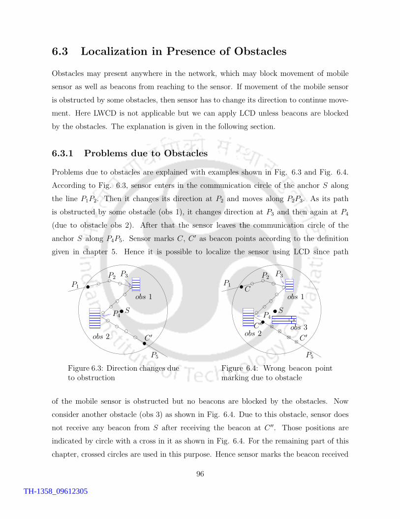
6.3 Localization in Presence of Obstacles
Obstacles may present anywhere in the network, which may block movement of mobile
sensor as well as beacons from reaching to the sensor. If movement of the mobile sensor
is obstructed by some obstacles, then sensor has to change its direction to continue move-
ment. Here LWCD is not applicable but we can apply LCD unless beacons are blocked
by the obstacles. The explanation is given in the following section.
6.3.1 Problems due to Obstacles
Problems due to obstacles are explained with examples shown in Fig. 6.3 and Fig. 6.4.
According to Fig. 6.3, sensor enters in the communication circle of the anchor S along
the line P1P2. Then it changes its direction at P2 and moves along P2P3. As its path
is obstructed by some obstacle (obs 1), it changes direction at P3 and then again at P4
(due to obstacle obs 2). After that the sensor leaves the communication circle of the
anchor S along P4P5. Sensor marks C, C ′ as beacon points according to the definition
given in chapter 5. Hence it is possible to localize the sensor using LCD since path
� � �� � �� � �� � �
� � �� � �� � �� � �
� � �� � �� � �� � �� � �� � �
� � �� � �� � �� � �� � �� � �
C ′
P1
P2P3
P4
P5
S
obs 1
obs 2
Figure 6.3: Direction changes dueto obstruction
� � � �� � � �� � � �� � � �� � � �
� � �� � �� � �� � �� � �
� � �� � �� � �
� � �� � �� � �
� � � � � �� � � � � �� � � � � �
C
C ′C ′′
P1
P2P3
P4
P5
S
obs 1
obs 2obs 3
Figure 6.4: Wrong beacon pointmarking due to obstacle
of the mobile sensor is obstructed but no beacons are blocked by the obstacles. Now
consider another obstacle (obs 3) as shown in Fig. 6.4. Due to this obstacle, sensor does
not receive any beacon from S after receiving the beacon at C ′′. Those positions are
indicated by circle with a cross in it as shown in Fig. 6.4. For the remaining part of this
chapter, crossed circles are used in this purpose. Hence sensor marks the beacon received
96
TH-1358_09612305
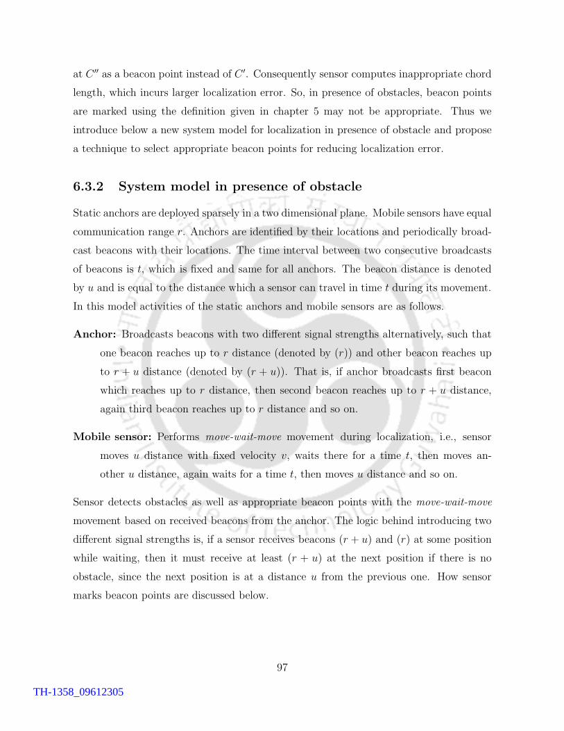
at C ′′ as a beacon point instead of C ′. Consequently sensor computes inappropriate chord
length, which incurs larger localization error. So, in presence of obstacles, beacon points
are marked using the definition given in chapter 5 may not be appropriate. Thus we
introduce below a new system model for localization in presence of obstacle and propose
a technique to select appropriate beacon points for reducing localization error.
6.3.2 System model in presence of obstacle
Static anchors are deployed sparsely in a two dimensional plane. Mobile sensors have equal
communication range r. Anchors are identified by their locations and periodically broad-
cast beacons with their locations. The time interval between two consecutive broadcasts
of beacons is t, which is fixed and same for all anchors. The beacon distance is denoted
by u and is equal to the distance which a sensor can travel in time t during its movement.
In this model activities of the static anchors and mobile sensors are as follows.
Anchor: Broadcasts beacons with two different signal strengths alternatively, such that
one beacon reaches up to r distance (denoted by (r)) and other beacon reaches up
to r + u distance (denoted by (r + u)). That is, if anchor broadcasts first beacon
which reaches up to r distance, then second beacon reaches up to r + u distance,
again third beacon reaches up to r distance and so on.
Mobile sensor: Performs move-wait-move movement during localization, i.e., sensor
moves u distance with fixed velocity v, waits there for a time t, then moves an-
other u distance, again waits for a time t, then moves u distance and so on.
Sensor detects obstacles as well as appropriate beacon points with the move-wait-move
movement based on received beacons from the anchor. The logic behind introducing two
different signal strengths is, if a sensor receives beacons (r + u) and (r) at some position
while waiting, then it must receive at least (r + u) at the next position if there is no
obstacle, since the next position is at a distance u from the previous one. How sensor
marks beacon points are discussed below.
97
TH-1358_09612305
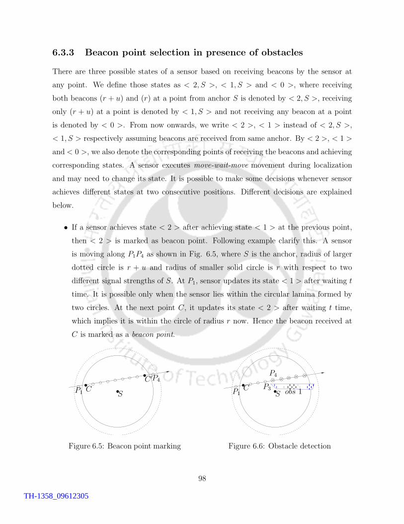
6.3.3 Beacon point selection in presence of obstacles
There are three possible states of a sensor based on receiving beacons by the sensor at
any point. We define those states as < 2, S >, < 1, S > and < 0 >, where receiving
both beacons (r + u) and (r) at a point from anchor S is denoted by < 2, S >, receiving
only (r + u) at a point is denoted by < 1, S > and not receiving any beacon at a point
is denoted by < 0 >. From now onwards, we write < 2 >, < 1 > instead of < 2, S >,
< 1, S > respectively assuming beacons are received from same anchor. By < 2 >, < 1 >
and < 0 >, we also denote the corresponding points of receiving the beacons and achieving
corresponding states. A sensor executes move-wait-move movement during localization
and may need to change its state. It is possible to make some decisions whenever sensor
achieves different states at two consecutive positions. Different decisions are explained
below.
• If a sensor achieves state < 2 > after achieving state < 1 > at the previous point,
then < 2 > is marked as beacon point. Following example clarify this. A sensor
is moving along P1P4 as shown in Fig. 6.5, where S is the anchor, radius of larger
dotted circle is r + u and radius of smaller solid circle is r with respect to two
different signal strengths of S. At P1, sensor updates its state < 1 > after waiting t
time. It is possible only when the sensor lies within the circular lamina formed by
two circles. At the next point C, it updates its state < 2 > after waiting t time,
which implies it is within the circle of radius r now. Hence the beacon received at
C is marked as a beacon point.
P1
P4
CC ′
S
Figure 6.5: Beacon point marking
� � � � � � � � � � � �� � � � � � � � � � � �
P1P3
P4
CS obs 1
Figure 6.6: Obstacle detection
98
TH-1358_09612305
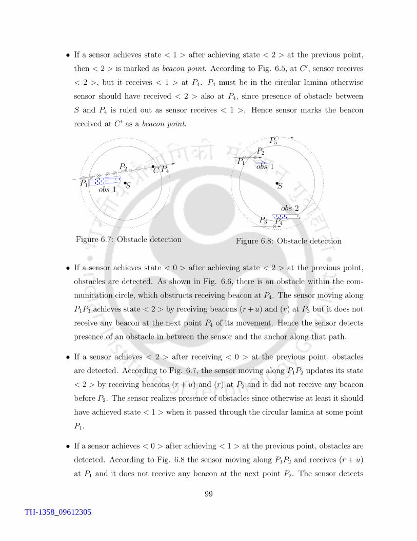
• If a sensor achieves state < 1 > after achieving state < 2 > at the previous point,
then < 2 > is marked as beacon point. According to Fig. 6.5, at C ′, sensor receives
< 2 >, but it receives < 1 > at P4. P4 must be in the circular lamina otherwise
sensor should have received < 2 > also at P4, since presence of obstacle between
S and P4 is ruled out as sensor receives < 1 >. Hence sensor marks the beacon
received at C ′ as a beacon point.
� � � � � � � �� � � � � � � �� � � � � � � �
P1
P2 P4C
Sobs 1
Figure 6.7: Obstacle detection
� � � � �� � � � �
� � � � � � �� � � � � � �
P1
P2
P3 P4
P5
S
obs 1
obs 2
Figure 6.8: Obstacle detection
• If a sensor achieves state < 0 > after achieving state < 2 > at the previous point,
obstacles are detected. As shown in Fig. 6.6, there is an obstacle within the com-
munication circle, which obstructs receiving beacon at P4. The sensor moving along
P1P3 achieves state < 2 > by receiving beacons (r+u) and (r) at P3 but it does not
receive any beacon at the next point P4 of its movement. Hence the sensor detects
presence of an obstacle in between the sensor and the anchor along that path.
• If a sensor achieves < 2 > after receiving < 0 > at the previous point, obstacles
are detected. According to Fig. 6.7, the sensor moving along P1P2 updates its state
< 2 > by receiving beacons (r+ u) and (r) at P2 and it did not receive any beacon
before P2. The sensor realizes presence of obstacles since otherwise at least it should
have achieved state < 1 > when it passed through the circular lamina at some point
P1.
• If a sensor achieves < 0 > after achieving < 1 > at the previous point, obstacles are
detected. According to Fig. 6.8 the sensor moving along P1P2 and receives (r + u)
at P1 and it does not receive any beacon at the next point P2. The sensor detects
99
TH-1358_09612305

presence of obstacle. Similar observation is also occur when a sensor moves along
P3P4 in the same figure. It may also be the case that the sensor is going out of the
larger circle after receiving beacon only at P5 as shown in Fig. 6.8.
• Sensor achieves < 1 > after achieving < 0 > implies sensor is in the circular lamina.
This happens at P1 in Fig. 6.5.
From above discussion we can say, sensor makes some decisions if it achieves different
states at two consecutive points. According to those decisions, sensor takes some actions
such that it can mark correct beacon points in presence of obstacles. Those decisions
and actions are shown in Table 6.1 where < a >→< b > implies a sensor changes state
to < b > from < a > at two consecutive positions. However, a sensor can change its
direction of movement if it achieves same state in two consecutive points. But like LCD,
it has to record time stamp whenever it changes direction.
Table 6.1: Decisions and actions taken by sensor after receiving two consecutive beaconswith different states to select correct beacon points in presence of obstacles
Case Decision Action
< 2 >→< 1 > < 2 > is a beacon point Sensor returns to previous po-sition, marks < 2 > as a bea-con point and changes direc-tion if needed
< 2 >→< 0 > Obstacle is detected Sensor returns to previous po-sition then changes directionand records time stamp simul-taneously
< 1 >→< 2 > < 2 > is a beacon point Sensor marks < 2 > as a bea-con point and continues move-ment along same direction
< 1 >→< 0 > Obstacle is detected or sensoris passing through the largercircle only
Sensor returns to previous po-sition then changes directionand records time stamp simul-taneously
< 0 >→< 1 > Sensor is in the circular lamina Sensor continues movementalong same direction
< 0 >→< 2 > Obstacle is detected Sensor continues movementalong same direction
100
TH-1358_09612305
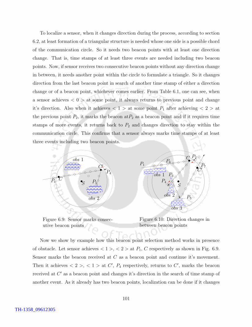
To localize a sensor, when it changes direction during the process, according to section
6.2, at least formation of a triangular structure is needed whose one side is a possible chord
of the communication circle. So it needs two beacon points with at least one direction
change. That is, time stamps of at least three events are needed including two beacon
points. Now, if sensor receives two consecutive beacon points without any direction change
in between, it needs another point within the circle to formulate a triangle. So it changes
direction from the last beacon point in search of another time stamp of either a direction
change or of a beacon point, whichever comes earlier. From Table 6.1, one can see, when
a sensor achieves < 0 > at some point, it always returns to previous point and change
it’s direction. Also when it achieves < 1 > at some point P1 after achieving < 2 > at
the previous point P2, it marks the beacon atP2 as a beacon point and if it requires time
stamps of more events, it returns back to P2 and changes direction to stay within the
communication circle. This confirms that a sensor always marks time stamps of at least
three events including two beacon points.
P1
P4
P5C
C ′
S
obs 1
obs 2
Figure 6.9: Sensor marks consec-utive beacon points
P1
P2
P3
P4
P5
P6P7
C
C ′
S
obs 1
obs 2
obs 3
Figure 6.10: Direction changes inbetween beacon points
Now we show by example how this beacon point selection method works in presence
of obstacle. Let sensor achieves < 1 >, < 2 > at P1, C respectively as shown in Fig. 6.9.
Sensor marks the beacon received at C as a beacon point and continue it’s movement.
Then it achieves < 2 >, < 1 > at C ′, P4 respectively, returns to C ′, marks the beacon
received at C ′ as a beacon point and changes it’s direction in the search of time stamp of
another event. As it already has two beacon points, localization can be done if it changes
101
TH-1358_09612305
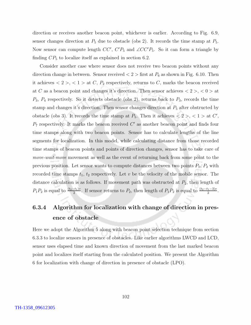
direction or receives another beacon point, whichever is earlier. According to Fig. 6.9,
sensor changes direction at P5 due to obstacle (obs 2). It records the time stamp at P5.
Now sensor can compute length CC ′, C ′P5 and ∠CC ′P5. So it can form a triangle by
finding CP5 to localize itself as explained in section 6.2.
Consider another case where sensor does not receive two beacon points without any
direction change in between. Sensor received < 2 > first at P6 as shown in Fig. 6.10. Then
it achieves < 2 >, < 1 > at C, P2 respectively, returns to C, marks the beacon received
at C as a beacon point and changes it’s direction. Then sensor achieves < 2 >, < 0 > at
P3, P4 respectively. So it detects obstacle (obs 2), returns back to P3, records the time
stamp and changes it’s direction. Then sensor changes direction at P5 after obstructed by
obstacle (obs 3). It records the time stamp at P5. Then it achieves < 2 >, < 1 > at C ′,
P7 respectively. It marks the beacon received C ′ as another beacon point and finds four
time stamps along with two beacon points. Sensor has to calculate lengths of the line
segments for localization. In this model, while calculating distance from those recorded
time stamps of beacon points and points of direction changes, sensor has to take care of
move-wait-move movement as well as the event of returning back from some point to the
previous position. Let sensor wants to compute distances between two points P1, P2 with
recorded time stamps t1, t2 respectively. Let v be the velocity of the mobile sensor. The
distance calculation is as follows. If movement path was obstructed at P2, then length of
P1P2 is equal to(t2−t1)v
2. If sensor returns to P2, then length of P1P2 is equal to
(t2−t1−3)v2
.
6.3.4 Algorithm for localization with change of direction in pres-
ence of obstacle
Here we adopt the Algorithm 5 along with beacon point selection technique from section
6.3.3 to localize sensors in presence of obstacles. Like earlier algorithms LWCD and LCD,
sensor uses elapsed time and known direction of movement from the last marked beacon
point and localizes itself starting from the calculated position. We present the Algorithm
6 for localization with change of direction in presence of obstacle (LPO).
102
TH-1358_09612305
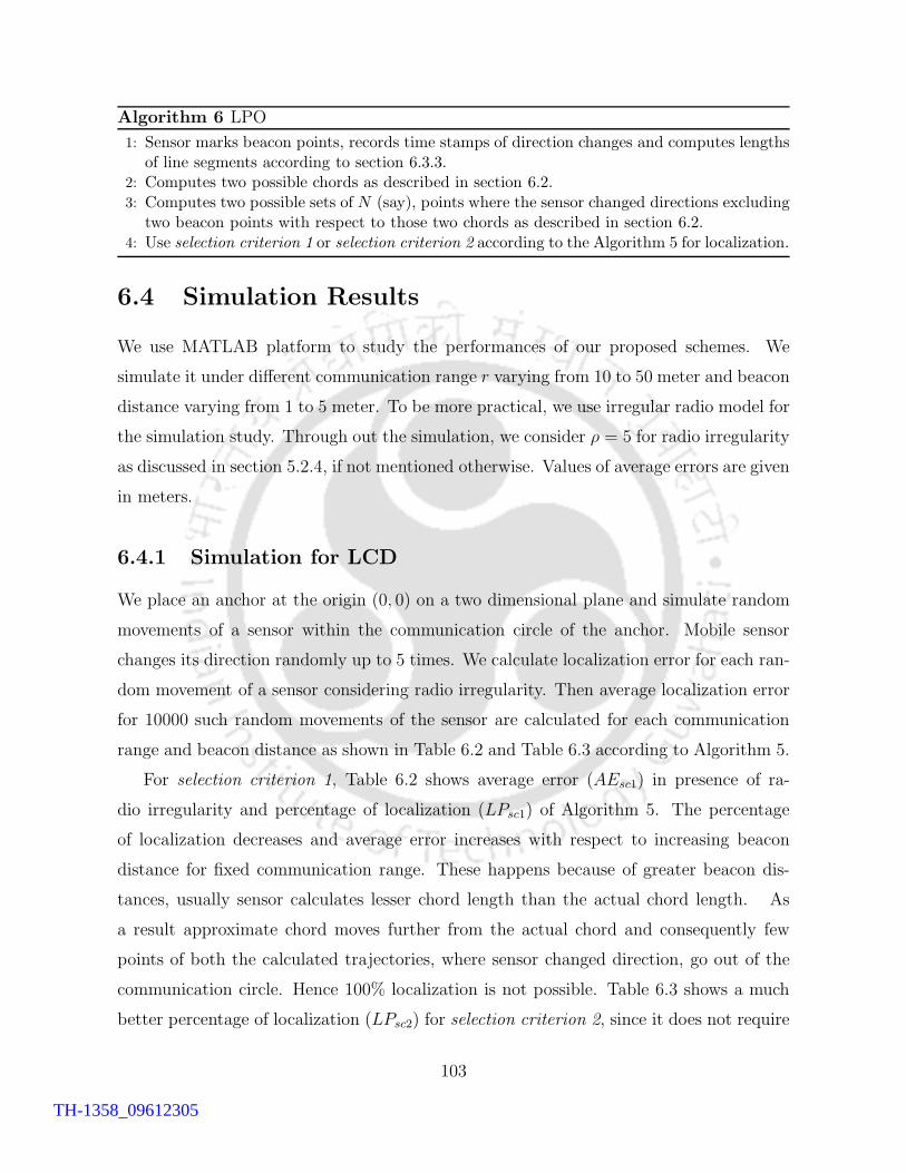
Algorithm 6 LPO
1: Sensor marks beacon points, records time stamps of direction changes and computes lengthsof line segments according to section 6.3.3.
2: Computes two possible chords as described in section 6.2.3: Computes two possible sets of N (say), points where the sensor changed directions excluding
two beacon points with respect to those two chords as described in section 6.2.4: Use selection criterion 1 or selection criterion 2 according to the Algorithm 5 for localization.
6.4 Simulation Results
We use MATLAB platform to study the performances of our proposed schemes. We
simulate it under different communication range r varying from 10 to 50 meter and beacon
distance varying from 1 to 5 meter. To be more practical, we use irregular radio model for
the simulation study. Through out the simulation, we consider ρ = 5 for radio irregularity
as discussed in section 5.2.4, if not mentioned otherwise. Values of average errors are given
in meters.
6.4.1 Simulation for LCD
We place an anchor at the origin (0, 0) on a two dimensional plane and simulate random
movements of a sensor within the communication circle of the anchor. Mobile sensor
changes its direction randomly up to 5 times. We calculate localization error for each ran-
dom movement of a sensor considering radio irregularity. Then average localization error
for 10000 such random movements of the sensor are calculated for each communication
range and beacon distance as shown in Table 6.2 and Table 6.3 according to Algorithm 5.
For selection criterion 1, Table 6.2 shows average error (AEsc1) in presence of ra-
dio irregularity and percentage of localization (LPsc1) of Algorithm 5. The percentage
of localization decreases and average error increases with respect to increasing beacon
distance for fixed communication range. These happens because of greater beacon dis-
tances, usually sensor calculates lesser chord length than the actual chord length. As
a result approximate chord moves further from the actual chord and consequently few
points of both the calculated trajectories, where sensor changed direction, go out of the
communication circle. Hence 100% localization is not possible. Table 6.3 shows a much
better percentage of localization (LPsc2) for selection criterion 2, since it does not require
103
TH-1358_09612305
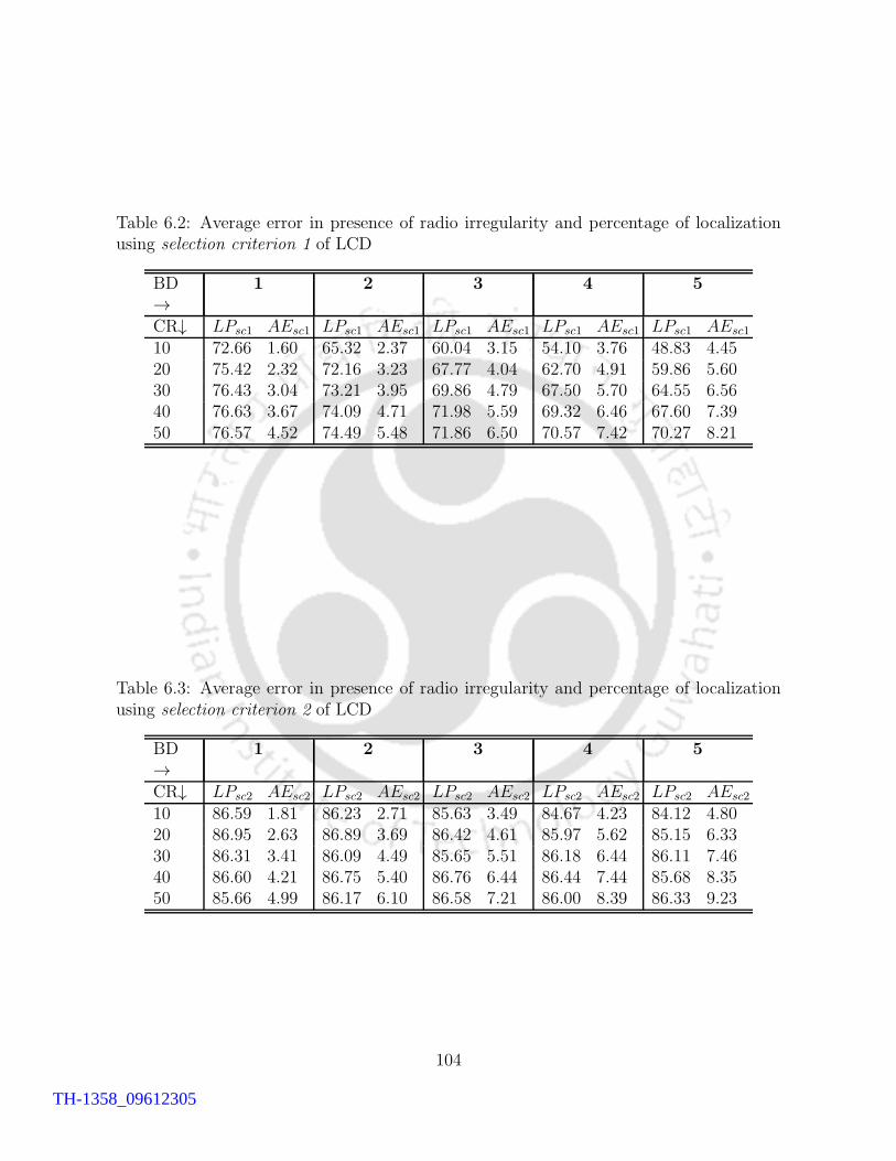
Table 6.2: Average error in presence of radio irregularity and percentage of localizationusing selection criterion 1 of LCD
BD→
1 2 3 4 5
CR↓ LPsc1 AEsc1 LPsc1 AEsc1 LPsc1 AEsc1 LPsc1 AEsc1 LPsc1 AEsc1
10 72.66 1.60 65.32 2.37 60.04 3.15 54.10 3.76 48.83 4.4520 75.42 2.32 72.16 3.23 67.77 4.04 62.70 4.91 59.86 5.6030 76.43 3.04 73.21 3.95 69.86 4.79 67.50 5.70 64.55 6.5640 76.63 3.67 74.09 4.71 71.98 5.59 69.32 6.46 67.60 7.3950 76.57 4.52 74.49 5.48 71.86 6.50 70.57 7.42 70.27 8.21
Table 6.3: Average error in presence of radio irregularity and percentage of localizationusing selection criterion 2 of LCD
BD→
1 2 3 4 5
CR↓ LPsc2 AEsc2 LPsc2 AEsc2 LPsc2 AEsc2 LPsc2 AEsc2 LPsc2 AEsc2
10 86.59 1.81 86.23 2.71 85.63 3.49 84.67 4.23 84.12 4.8020 86.95 2.63 86.89 3.69 86.42 4.61 85.97 5.62 85.15 6.3330 86.31 3.41 86.09 4.49 85.65 5.51 86.18 6.44 86.11 7.4640 86.60 4.21 86.75 5.40 86.76 6.44 86.44 7.44 85.68 8.3550 85.66 4.99 86.17 6.10 86.58 7.21 86.00 8.39 86.33 9.23
104
TH-1358_09612305
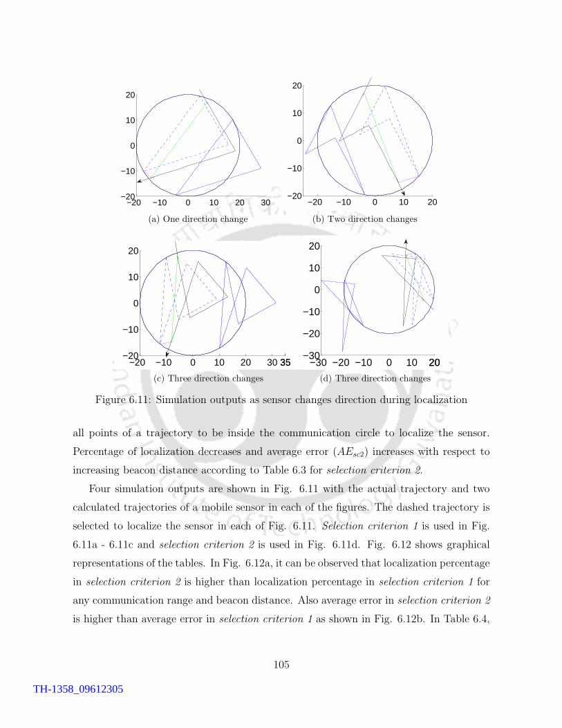
−20 −10 0 10 20 30−20
−10
0
10
20
(a) One direction change
−20 −10 0 10 20−20
−10
0
10
20
(b) Two direction changes
−20 −10 0 10 20 30 3535−20
−10
0
10
20
(c) Three direction changes
−30 −20 −10 0 10 2020−30
−20
−10
0
10
20
(d) Three direction changes
Figure 6.11: Simulation outputs as sensor changes direction during localization
all points of a trajectory to be inside the communication circle to localize the sensor.
Percentage of localization decreases and average error (AEsc2) increases with respect to
increasing beacon distance according to Table 6.3 for selection criterion 2.
Four simulation outputs are shown in Fig. 6.11 with the actual trajectory and two
calculated trajectories of a mobile sensor in each of the figures. The dashed trajectory is
selected to localize the sensor in each of Fig. 6.11. Selection criterion 1 is used in Fig.
6.11a - 6.11c and selection criterion 2 is used in Fig. 6.11d. Fig. 6.12 shows graphical
representations of the tables. In Fig. 6.12a, it can be observed that localization percentage
in selection criterion 2 is higher than localization percentage in selection criterion 1 for
any communication range and beacon distance. Also average error in selection criterion 2
is higher than average error in selection criterion 1 as shown in Fig. 6.12b. In Table 6.4,
105
TH-1358_09612305

12
34
55
10203040505030
50
70
90
Beacon distance (m)
Communication range (m)
Loca
lizat
ion
Per
cent
age
(%)
LPsc2
LPsc1
(a) Localization percentage with respectto selection criterion 1 & 2
1 2 3 4 55
10203040505002468
10
Beacon distance (m)
Communication range (m)
Ave
rage
err
or (
m)
AEsc2
AEsc1
(b) Average error with respect to selection
criterion 1 & 2
Figure 6.12: Performance of selection criterion 1 and selection criterion 2
0 5 10 15 200
1
2
3
4
5
6
7
ρ
Ave
rage
err
or(m
)
Selection criterion 1Selection criterion 2
Figure 6.13: Average errors of LCD versus radio irregularity ρ
we compare our proposed algorithm with existing algorithms. Simulation results show
around 67% and 63% improvement over WMCL-A for selection criterion 1 and selection
criterion 2 of LCD respectively in terms of average localization error.
Table 6.4: Average error (r) of our proposed algorithm compared LCD with some existingalgorithms, where r is the communication range of anchor
Algorithm LCD WMCL-A WMCL-B MCB MCLselection selectioncriterion 1 criterion 2
Error(r) 0.165 0.185 0.503 0.568 0.662 0.766
In Fig. 6.13, we show a two dimensional plot of AEsc1 and AEsc2 versus ρ, where ρ is
varying from 0 to 20. Here communication range and beacon distance are 20 meter and 2
meter respectively. AEsc1 is varying from 2.3 meter to 5.6 meter whereas AEsc2 is varying
from 2.7 meter to 6.3 meter according to the figure.
106
TH-1358_09612305
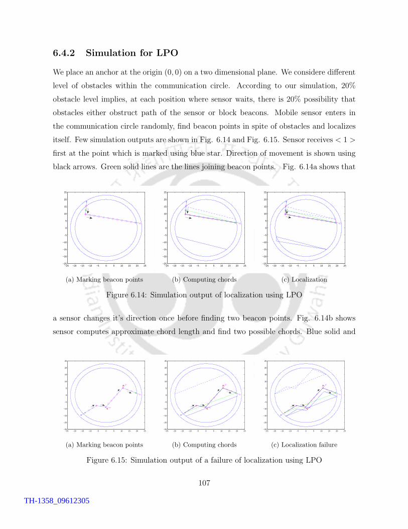
6.4.2 Simulation for LPO
We place an anchor at the origin (0, 0) on a two dimensional plane. We considere different
level of obstacles within the communication circle. According to our simulation, 20%
obstacle level implies, at each position where sensor waits, there is 20% possibility that
obstacles either obstruct path of the sensor or block beacons. Mobile sensor enters in
the communication circle randomly, find beacon points in spite of obstacles and localizes
itself. Few simulation outputs are shown in Fig. 6.14 and Fig. 6.15. Sensor receives < 1 >
first at the point which is marked using blue star. Direction of movement is shown using
black arrows. Green solid lines are the lines joining beacon points. Fig. 6.14a shows that
−25 −20 −15 −10 −5 0 5 10 15 20 25−25
−20
−15
−10
−5
0
5
10
15
20
25
(a) Marking beacon points
−25 −20 −15 −10 −5 0 5 10 15 20 25−25
−20
−15
−10
−5
0
5
10
15
20
25
(b) Computing chords
−25 −20 −15 −10 −5 0 5 10 15 20 25−25
−20
−15
−10
−5
0
5
10
15
20
25
(c) Localization
Figure 6.14: Simulation output of localization using LPO
a sensor changes it’s direction once before finding two beacon points. Fig. 6.14b shows
sensor computes approximate chord length and find two possible chords. Blue solid and
−25 −20 −15 −10 −5 0 5 10 15 20 25−25
−20
−15
−10
−5
0
5
10
15
20
25
(a) Marking beacon points
−25 −20 −15 −10 −5 0 5 10 15 20 25−25
−20
−15
−10
−5
0
5
10
15
20
25
(b) Computing chords
−25 −20 −15 −10 −5 0 5 10 15 20 25−25
−20
−15
−10
−5
0
5
10
15
20
25
(c) Localization failure
Figure 6.15: Simulation output of a failure of localization using LPO
107
TH-1358_09612305
Table 6.5: Average error in presence of radio irregularity and percentage of localizationusing selection criterion 1 of LPO for 20% obstacle level
BD→
1 2 3 4 5
CR↓ LPsc1 AEsc1 LPsc1 AEsc1 LPsc1 AEsc1 LPsc1 AEsc1 LPsc1 AEsc1
10 75.70 2.72 68.30 3.26 63.20 4.46 53.50 5.24 44.00 6.2720 69.30 3.74 65.0 4.80 62.70 5.81 65.70 7.04 63.50 7.7930 61.30 5.92 63.20 6.58 61.60 7.83 63.40 7.97 62.60 9.8140 54.20 11.14 58.60 8.40 61.50 9.15 57.70 9.43 59.30 11.3250 45.50 13.50 54.80 9.49 59.90 11.16 53.10 11.72 57.10 11.29
blue dotted lines show two approximate chords with same length and gradient. Finally
in Fig. 6.14c, sensor finds that the blue dotted trajectory is within the circle of radius r
centering at the anchor and localizes accordingly. Fig. 6.15 shows failure of localization.
Sensor changes direction thrice before finding two beacon points in Fig. 6.15a. For the
last two direction changes, sensor returns back to previous positions and then changes
direction which happened due to receiving no beacon at those points. Returning back to
previous positions are shown using red dotted arrows. Fig. 6.15b shows sensor computes
approximate chord length and find two possible chords. Blue solid and blue dotted lines
show two approximate chords with same length and gradient. In Fig. 6.15c, sensor finds
both the trajectories are entirely within the circle with radius r centering at the anchor,
hence localization can not be done.
We calculate localization error for each run of LPO by a sensor considering radio irreg-
ularity. Average localization error for 10000 such runs for each communication range and
beacon distance are calculated as shown in Table 6.5 and Table 6.6 according to Algorithm
6. For selection criterion 1, Table 6.5 shows average error (AEsc1) in presence of radio ir-
regularity and percentage of localization (LPsc1) of Algorithm 6 considering 20% obstacle
level. For selection criterion 2, Table 6.6 shows average error (AEsc2) in presence of radio
irregularity and percentage of localization (LPsc2) of Algorithm 6 considering 20% obsta-
cle level. In most of the cases, average localization errors increase as communication range
increases for any fixed beacon distance in both Tables 6.5 and 6.6. In most of the cases,
percentage of localization (LPsc1) for selection criterion 1 in Table 6.5 decreases as com-
munication range increases for any fixed beacon distance. On the other hand, percentage
108
TH-1358_09612305
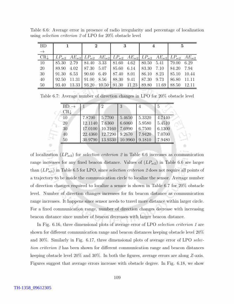
Table 6.6: Average error in presence of radio irregularity and percentage of localizationusing selection criterion 2 of LPO for 20% obstacle level
BD→
1 2 3 4 5
CR↓ LPsc2 AEsc2 LPsc2 AEsc2 LPsc2 AEsc2 LPsc2 AEsc2 LPsc2 AEsc2
10 85.30 2.79 84.40 3.33 81.60 4.62 80.50 5.41 79.00 6.2920 89.90 4.02 87.30 5.07 85.60 6.14 83.30 7.10 84.20 7.9430 91.30 6.53 90.60 6.49 87.40 8.01 86.10 8.23 85.10 10.4440 92.50 11.31 91.00 8.56 88.30 9.41 87.30 9.73 86.80 11.1150 93.40 13.33 93.20 10.50 91.30 11.23 89.80 11.69 88.50 12.11
Table 6.7: Average number of direction changes in LPO for 20% obstacle level
BD → 1 2 3 4 5CR↓10 7.8700 5.7700 5.4650 5.3320 4.744020 12.1140 7.6360 6.6060 5.9580 5.451030 17.0100 10.2160 7.6990 6.7500 6.130040 22.4360 12.7290 9.2670 7.9420 7.070050 30.9790 13.9330 10.9960 9.1810 7.9480
of localization (LPsc2) for selection criterion 2 in Table 6.6 increases as communication
range increases for any fixed beacon distance. Values of (LPsc2) in Table 6.6 are larger
than (LPsc1) in Table 6.5 for LPO, since selection criterion 2 does not require all points of
a trajectory to be inside the communication circle to localize the sensor. Average number
of direction changes required to localize a sensor is shown in Table 6.7 for 20% obstacle
level. Number of direction changes increases for fix beacon distance as communication
range increases. It happens since sensor needs to travel more distance within larger circle.
For a fixed communication range, number of direction changes decrease with increasing
beacon distance since number of beacon decreases with larger beacon distance.
In Fig. 6.16, three dimensional plots of average error of LPO selection criterion 1 are
shown for different communication range and beacon distances keeping obstacle level 20%
and 30%. Similarly in Fig. 6.17, three dimensional plots of average error of LPO selec-
tion criterion 2 has been shown for different communication range and beacon distances
keeping obstacle level 20% and 30%. In both the figures, average errors are along Z-axis.
Figures suggest that average errors increase with obstacle degree. In Fig. 6.18, we show
109
TH-1358_09612305
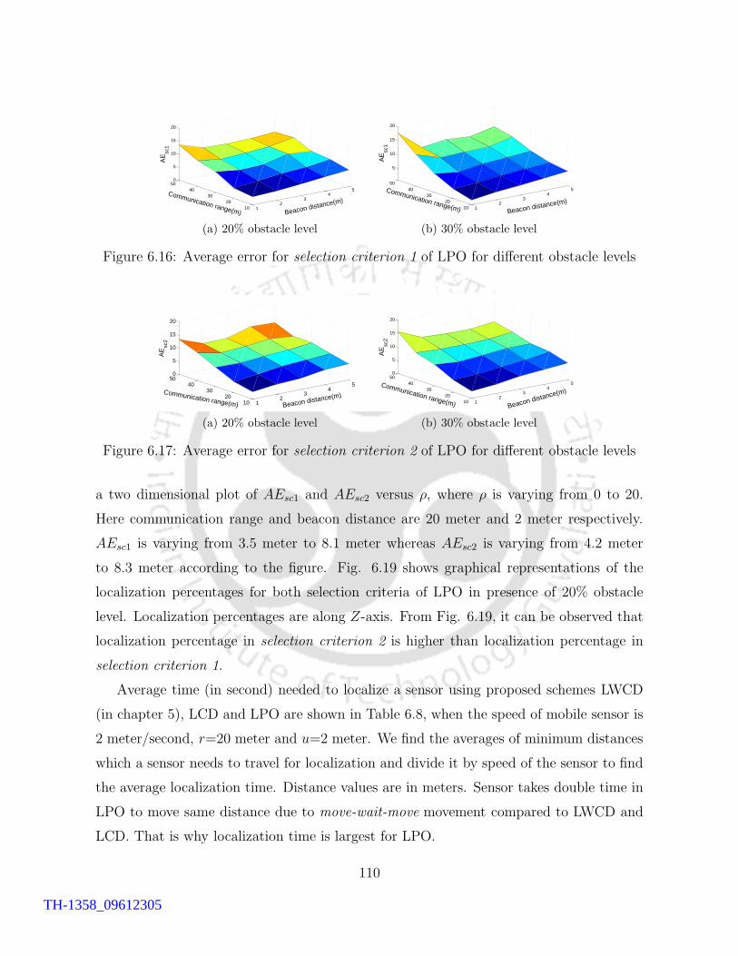
12
34
5
1020
3040
500
5
10
15
20
Beacon distance(m)Communication range(m)
AE
sc1
(a) 20% obstacle level
12
34
5
1020
3040
50
5
10
15
20
Beacon distance(m)
Communication range(m)
AE
sc1
(b) 30% obstacle level
Figure 6.16: Average error for selection criterion 1 of LPO for different obstacle levels
12
34
5
1020
3040
500
5
10
15
20
Beacon distance(m)Communication range(m)
AE
sc2
(a) 20% obstacle level
12
34
5
1020
3040
500
5
10
15
20
Beacon distance(m)Communication range(m)
AE
sc2
(b) 30% obstacle level
Figure 6.17: Average error for selection criterion 2 of LPO for different obstacle levels
a two dimensional plot of AEsc1 and AEsc2 versus ρ, where ρ is varying from 0 to 20.
Here communication range and beacon distance are 20 meter and 2 meter respectively.
AEsc1 is varying from 3.5 meter to 8.1 meter whereas AEsc2 is varying from 4.2 meter
to 8.3 meter according to the figure. Fig. 6.19 shows graphical representations of the
localization percentages for both selection criteria of LPO in presence of 20% obstacle
level. Localization percentages are along Z-axis. From Fig. 6.19, it can be observed that
localization percentage in selection criterion 2 is higher than localization percentage in
selection criterion 1.
Average time (in second) needed to localize a sensor using proposed schemes LWCD
(in chapter 5), LCD and LPO are shown in Table 6.8, when the speed of mobile sensor is
2 meter/second, r=20 meter and u=2 meter. We find the averages of minimum distances
which a sensor needs to travel for localization and divide it by speed of the sensor to find
the average localization time. Distance values are in meters. Sensor takes double time in
LPO to move same distance due to move-wait-move movement compared to LWCD and
LCD. That is why localization time is largest for LPO.
110
TH-1358_09612305
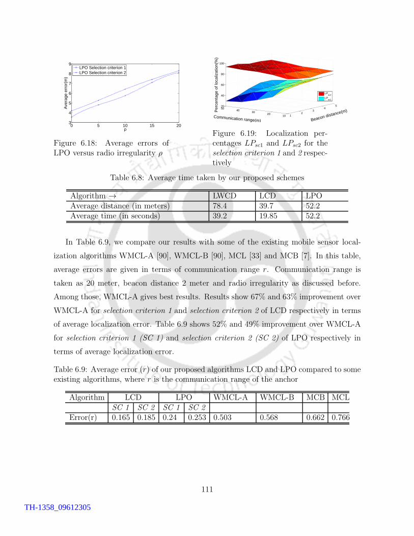
0 5 10 15 203
4
5
6
7
8
9
ρ
Ave
rage
err
or(m
)
LPO Selection criterion 1LPO Selection criterion 2
Figure 6.18: Average errors ofLPO versus radio irregularity ρ
12
34
5
1020
3040
5020
40
60
80
100
Beacon distance(m)Communication range(m)
Per
cent
age
of lo
caliz
atio
n(%
)
LPsc2
LPsc1
Figure 6.19: Localization per-centages LPsc1 and LPsc2 for theselection criterion 1 and 2 respec-tively
Table 6.8: Average time taken by our proposed schemes
Algorithm → LWCD LCD LPOAverage distance (in meters) 78.4 39.7 52.2Average time (in seconds) 39.2 19.85 52.2
In Table 6.9, we compare our results with some of the existing mobile sensor local-
ization algorithms WMCL-A [90], WMCL-B [90], MCL [33] and MCB [7]. In this table,
average errors are given in terms of communication range r. Communication range is
taken as 20 meter, beacon distance 2 meter and radio irregularity as discussed before.
Among those, WMCL-A gives best results. Results show 67% and 63% improvement over
WMCL-A for selection criterion 1 and selection criterion 2 of LCD respectively in terms
of average localization error. Table 6.9 shows 52% and 49% improvement over WMCL-A
for selection criterion 1 (SC 1) and selection criterion 2 (SC 2) of LPO respectively in
terms of average localization error.
Table 6.9: Average error (r) of our proposed algorithms LCD and LPO compared to someexisting algorithms, where r is the communication range of the anchor
Algorithm LCD LPO WMCL-A WMCL-B MCB MCLSC 1 SC 2 SC 1 SC 2
Error(r) 0.165 0.185 0.24 0.253 0.503 0.568 0.662 0.766
111
TH-1358_09612305

6.5 Conclusion
In this chapter we have proposed LCD for localization considering sensors change direction
while localization. Another algorithm LPO is proposed which localizes sensors in presence
of obstacles. LPO selects appropriate beacon points in presence of obstacles using a
different system model. Simulation results of LPO show good positioning accuracy for
different levels of obstacles. Better positioning accuracy is observed in simulation for LCD
and LPO compared to existing works.
112
TH-1358_09612305

Chapter 7
Path Planning for Mobile Anchor in
Connected Networks
7.1 Introduction
A number of static anchors are used to localize static senors in the localization schemes [14,
20, 68, 92]. To minimize the number of static anchors and to avoid range measurements,
range-free localization schemes [46, 75, 84] using mobile anchor are proposed. One mobile
anchor with a suitable path planning is equivalent to many static anchors, which localizes
whole network. By a single mobile anchor we can save large number of static anchors with
deployment cost in the expense of the mobility of the mobile anchor. Therefore, reducing
path length of the mobile anchor becomes an important issue in the area of localization.
Range measurements are done in most of the existing works [47, 48, 36], where path
planning are proposed for connected network. Our aim is to propose a path planning
using only connectivity information which can adapt an existing range-free localization
scheme for better accuracy. In this chapter we propose a movement strategy for a mobile
anchor to localize sensors of a connected network with connectivity guided movement.
We use range-free localization scheme proposed by Lee et al. [46] which yields better
positioning accuracy.
113
TH-1358_09612305
7.1.1 Our contribution
We introduce a hexagonal movement strategy for mobile anchors. Our proposed dis-
tributed range-free movement strategy localizes all sensors within r/2 error-bound in a
connected network, where r is the transmission range of the sensors and the mobile anchor.
To the best of our knowledge, this is the first work where localization and path planning
both are done using connectivity of the network without range estimation. Simulation
results show improvement over existing work [48] in terms of both path length and local-
ization accuracy. Full localization is guaranteed in absence of irregular radio propagation.
Simulation results show, also in presence of radio irregularity, all the sensors are being
localized using proposed movement strategy.
The organization of the remaining part of this work is as follows. The theoretical
results of our proposed path planning on a connected network are explained in section
7.2. The algorithm along with system model and correctness proof, complexity analysis
are given in section 7.3. Effect of irregular radio propagation is discussed in section 7.4.
The simulation results are presented in section 7.5. Finally we conclude in section 7.6.
7.2 Path Planning
In this section we discuss path planning to localize an arbitrary connected network of any
number of sensors. The mobile anchor broadcasts beacon with its position information
after every t time interval. We may use the term ‘anchor’ instead of ‘mobile anchor’ in
the rest part of this paper.
Definition 7.2.1. (Beacon distance) Distance traveled by the mobile anchor between two
consecutive broadcasts of beacon is called beacon distance and is denoted by u.
Definition 7.2.2. (Communication circle) The circle with radius r centering at the sen-
sor, where r is the communication range of the sensor.
Definition 7.2.3. (LRH) Largest regular hexagon inscribed within the communication
circle of any sensor.
Definition 7.2.4. (Beacon point) The position of the anchor that is extracted from the
beacon received by a sensor at time x is denoted as a beacon point for the sensor if and
114
TH-1358_09612305
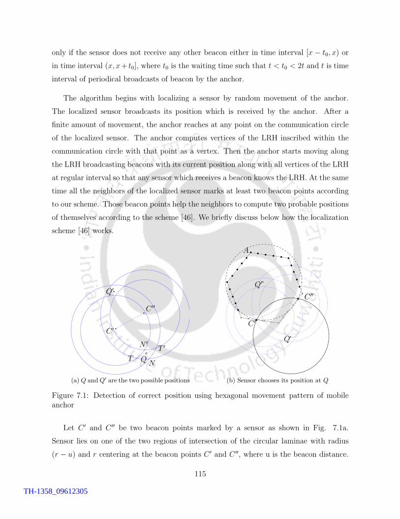
only if the sensor does not receive any other beacon either in time interval [x − t0, x) or
in time interval (x, x+ t0], where t0 is the waiting time such that t < t0 < 2t and t is time
interval of periodical broadcasts of beacon by the anchor.
The algorithm begins with localizing a sensor by random movement of the anchor.
The localized sensor broadcasts its position which is received by the anchor. After a
finite amount of movement, the anchor reaches at any point on the communication circle
of the localized sensor. The anchor computes vertices of the LRH inscribed within the
communication circle with that point as a vertex. Then the anchor starts moving along
the LRH broadcasting beacons with its current position along with all vertices of the LRH
at regular interval so that any sensor which receives a beacon knows the LRH. At the same
time all the neighbors of the localized sensor marks at least two beacon points according
to our scheme. Those beacon points help the neighbors to compute two probable positions
of themselves according to the scheme [46]. We briefly discuss below how the localization
scheme [46] works.
C ′
C ′′
T
T ′
Q
Q′
N
N ′
(a)Q andQ′ are the two possible positions
A
C ′
C ′′
Q
Q′
(b) Sensor chooses its position at Q
Figure 7.1: Detection of correct position using hexagonal movement pattern of mobileanchor
Let C ′ and C ′′ be two beacon points marked by a sensor as shown in Fig. 7.1a.
Sensor lies on one of the two regions of intersection of the circular laminae with radius
(r − u) and r centering at the beacon points C ′ and C ′′, where u is the beacon distance.
115
TH-1358_09612305
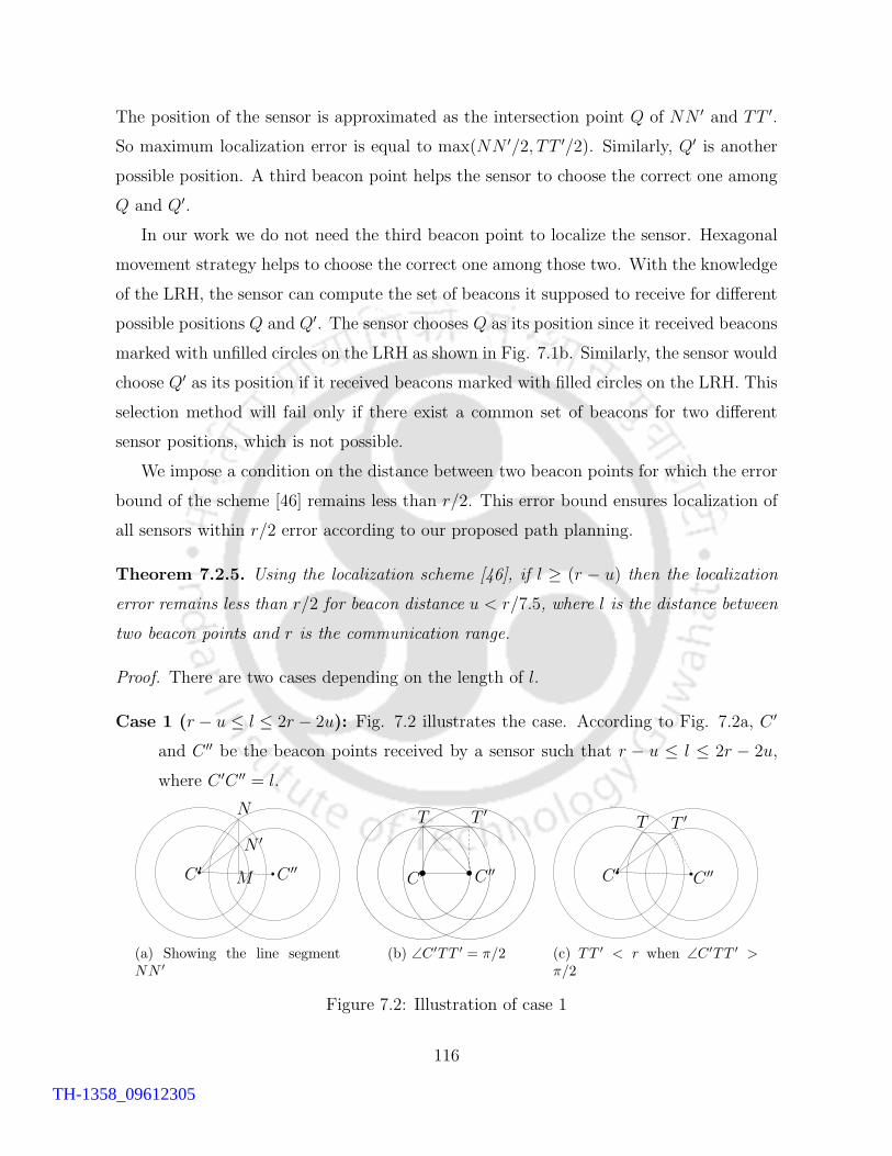
The position of the sensor is approximated as the intersection point Q of NN ′ and TT ′.
So maximum localization error is equal to max(NN ′/2, TT ′/2). Similarly, Q′ is another
possible position. A third beacon point helps the sensor to choose the correct one among
Q and Q′.
In our work we do not need the third beacon point to localize the sensor. Hexagonal
movement strategy helps to choose the correct one among those two. With the knowledge
of the LRH, the sensor can compute the set of beacons it supposed to receive for different
possible positions Q and Q′. The sensor chooses Q as its position since it received beacons
marked with unfilled circles on the LRH as shown in Fig. 7.1b. Similarly, the sensor would
choose Q′ as its position if it received beacons marked with filled circles on the LRH. This
selection method will fail only if there exist a common set of beacons for two different
sensor positions, which is not possible.
We impose a condition on the distance between two beacon points for which the error
bound of the scheme [46] remains less than r/2. This error bound ensures localization of
all sensors within r/2 error according to our proposed path planning.
Theorem 7.2.5. Using the localization scheme [46], if l ≥ (r − u) then the localization
error remains less than r/2 for beacon distance u < r/7.5, where l is the distance between
two beacon points and r is the communication range.
Proof. There are two cases depending on the length of l.
Case 1 (r − u ≤ l ≤ 2r − 2u): Fig. 7.2 illustrates the case. According to Fig. 7.2a, C ′
and C ′′ be the beacon points received by a sensor such that r − u ≤ l ≤ 2r − 2u,
where C ′C ′′ = l.
C ′ C ′′
N
N ′
M
(a) Showing the line segmentNN ′
C ′ C ′′
T T ′
(b) ∠C′TT ′ = π/2
C ′C ′′
T T ′
(c) TT ′ < r when ∠C′TT ′ >π/2
Figure 7.2: Illustration of case 1
116
TH-1358_09612305
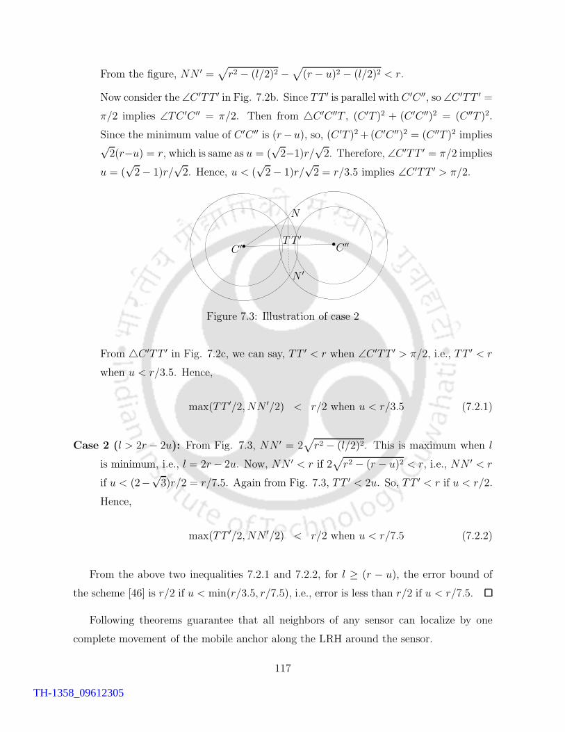
From the figure, NN ′ =√
r2 − (l/2)2 −√
(r − u)2 − (l/2)2 < r.
Now consider the ∠C ′TT ′ in Fig. 7.2b. Since TT ′ is parallel with C ′C ′′, so ∠C ′TT ′ =
π/2 implies ∠TC ′C ′′ = π/2. Then from 4C ′C ′′T , (C ′T )2 + (C ′C ′′)2 = (C ′′T )2.
Since the minimum value of C ′C ′′ is (r−u), so, (C ′T )2+(C ′C ′′)2 = (C ′′T )2 implies√2(r−u) = r, which is same as u = (
√2−1)r/
√2. Therefore, ∠C ′TT ′ = π/2 implies
u = (√2− 1)r/
√2. Hence, u < (
√2− 1)r/
√2 = r/3.5 implies ∠C ′TT ′ > π/2.
C ′ C ′′T T ′
N
N ′
Figure 7.3: Illustration of case 2
From 4C ′TT ′ in Fig. 7.2c, we can say, TT ′ < r when ∠C ′TT ′ > π/2, i.e., TT ′ < r
when u < r/3.5. Hence,
max(TT ′/2, NN ′/2) < r/2 when u < r/3.5 (7.2.1)
Case 2 (l > 2r − 2u): From Fig. 7.3, NN ′ = 2√
r2 − (l/2)2. This is maximum when l
is minimum, i.e., l = 2r− 2u. Now, NN ′ < r if 2√
r2 − (r − u)2 < r, i.e., NN ′ < r
if u < (2−√3)r/2 = r/7.5. Again from Fig. 7.3, TT ′ < 2u. So, TT ′ < r if u < r/2.
Hence,
max(TT ′/2, NN ′/2) < r/2 when u < r/7.5 (7.2.2)
From the above two inequalities 7.2.1 and 7.2.2, for l ≥ (r − u), the error bound of
the scheme [46] is r/2 if u < min(r/3.5, r/7.5), i.e., error is less than r/2 if u < r/7.5.
Following theorems guarantee that all neighbors of any sensor can localize by one
complete movement of the mobile anchor along the LRH around the sensor.
117
TH-1358_09612305
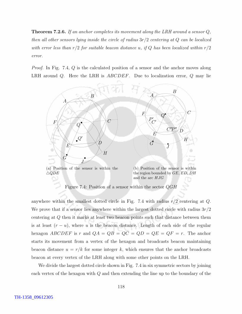
Theorem 7.2.6. If an anchor completes its movement along the LRH around a sensor Q,
then all other sensors lying inside the circle of radius 3r/2 centering at Q can be localized
with error less than r/2 for suitable beacon distance u, if Q has been localized within r/2
error.
Proof. In Fig. 7.4, Q is the calculated position of a sensor and the anchor moves along
LRH around Q. Here the LRH is ABCDEF . Due to localization error, Q may lie
AB
C
DE
F
GH
J
Q′
Q
(a) Position of the sensor is within the4QDE
AB
C
D
C ′
C ′′
E
F
GH
J
P ′
P ′′
Q
(b) Position of the sensor is withinthe region bounded by GE, ED, DHand the arc HJG
Figure 7.4: Position of a sensor within the sector QGH
anywhere within the smallest dotted circle in Fig. 7.4 with radius r/2 centering at Q.
We prove that if a sensor lies anywhere within the largest dotted circle with radius 3r/2
centering at Q then it marks at least two beacon points such that distance between them
is at least (r − u), where u is the beacon distance. Length of each side of the regular
hexagon ABCDEF is r and QA = QB = QC = QD = QE = QF = r. The anchor
starts its movement from a vertex of the hexagon and broadcasts beacon maintaining
beacon distance u = r/k for some integer k, which ensures that the anchor broadcasts
beacon at every vertex of the LRH along with some other points on the LRH.
We divide the largest dotted circle shown in Fig. 7.4 in six symmetric sectors by joining
each vertex of the hexagon with Q and then extending the line up to the boundary of the
118
TH-1358_09612305
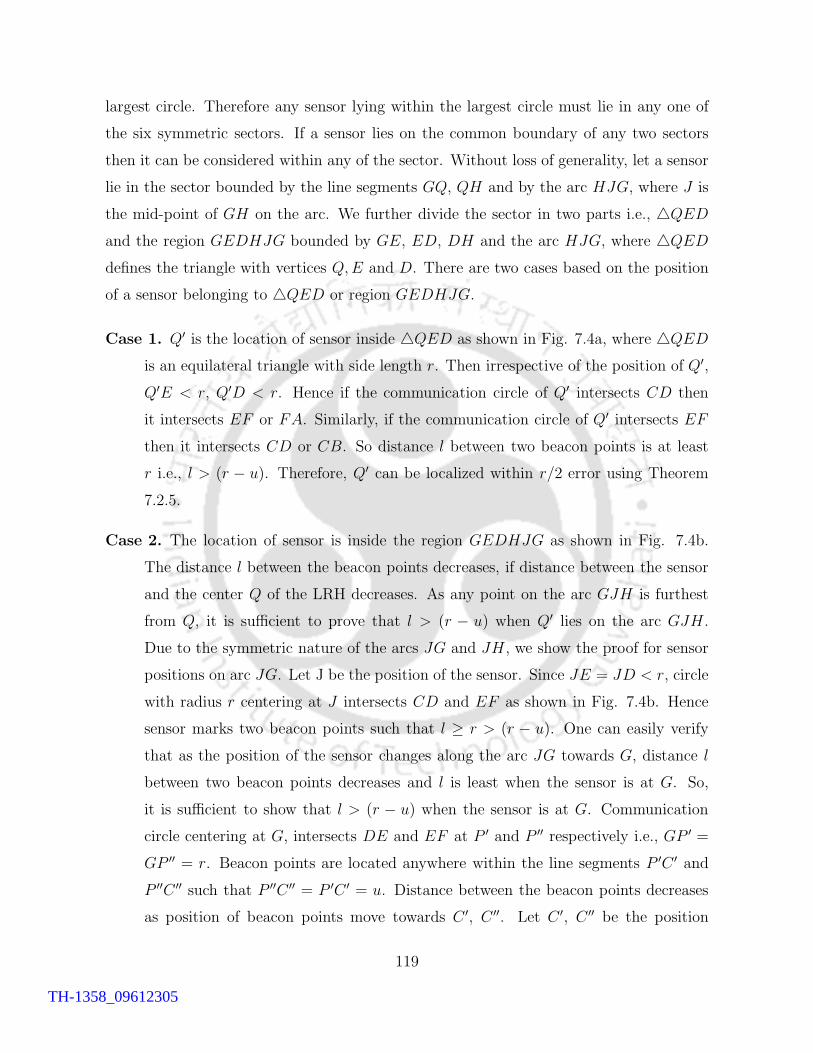
largest circle. Therefore any sensor lying within the largest circle must lie in any one of
the six symmetric sectors. If a sensor lies on the common boundary of any two sectors
then it can be considered within any of the sector. Without loss of generality, let a sensor
lie in the sector bounded by the line segments GQ, QH and by the arc HJG, where J is
the mid-point of GH on the arc. We further divide the sector in two parts i.e., 4QED
and the region GEDHJG bounded by GE, ED, DH and the arc HJG, where 4QED
defines the triangle with vertices Q,E and D. There are two cases based on the position
of a sensor belonging to 4QED or region GEDHJG.
Case 1. Q′ is the location of sensor inside 4QED as shown in Fig. 7.4a, where 4QED
is an equilateral triangle with side length r. Then irrespective of the position of Q′,
Q′E < r, Q′D < r. Hence if the communication circle of Q′ intersects CD then
it intersects EF or FA. Similarly, if the communication circle of Q′ intersects EF
then it intersects CD or CB. So distance l between two beacon points is at least
r i.e., l > (r − u). Therefore, Q′ can be localized within r/2 error using Theorem
7.2.5.
Case 2. The location of sensor is inside the region GEDHJG as shown in Fig. 7.4b.
The distance l between the beacon points decreases, if distance between the sensor
and the center Q of the LRH decreases. As any point on the arc GJH is furthest
from Q, it is sufficient to prove that l > (r − u) when Q′ lies on the arc GJH .
Due to the symmetric nature of the arcs JG and JH , we show the proof for sensor
positions on arc JG. Let J be the position of the sensor. Since JE = JD < r, circle
with radius r centering at J intersects CD and EF as shown in Fig. 7.4b. Hence
sensor marks two beacon points such that l ≥ r > (r − u). One can easily verify
that as the position of the sensor changes along the arc JG towards G, distance l
between two beacon points decreases and l is least when the sensor is at G. So,
it is sufficient to show that l > (r − u) when the sensor is at G. Communication
circle centering at G, intersects DE and EF at P ′ and P ′′ respectively i.e., GP ′ =
GP ′′ = r. Beacon points are located anywhere within the line segments P ′C ′ and
P ′′C ′′ such that P ′′C ′′ = P ′C ′ = u. Distance between the beacon points decreases
as position of beacon points move towards C ′, C ′′. Let C ′, C ′′ be the position
119
TH-1358_09612305
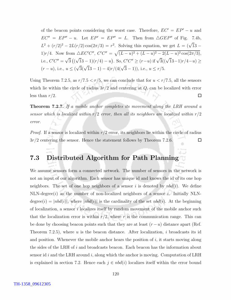
of the beacon points considering the worst case. Therefore, EC ′ = EP ′ − u and
EC ′′ = EP ′′ − u. Let EP ′ = EP ′′ = L. Then from 4GEP ′′ of Fig. 7.4b,
L2 + (r/2)2 − 2L(r/2) cos(2π/3) = r2. Solving this equation, we get L = (√13 −
1)r/4. Now from 4EC ′C ′′, C ′C ′′ =√
(L− u)2 + (L− u)2 − 2(L− u)2 cos(2π/3),
i.e., C ′C ′′ =√3(
(√13− 1)(r/4)− u
)
. So, C ′C ′′ ≥ (r−u) if√3((
√13−1)r/4−u) ≥
(r − u), i.e., u ≤ (√3(√13− 1)− 4)r/(4(
√3− 1)), i.e., u ≤ r/5.
Using Theorem 7.2.5, as r/7.5 < r/5, we can conclude that for u < r/7.5, all the sensors
which lie within the circle of radius 3r/2 and centering at Q, can be localized with error
less than r/2.
Theorem 7.2.7. If a mobile anchor completes its movement along the LRH around a
sensor which is localized within r/2 error, then all its neighbors are localized within r/2
error.
Proof. If a sensor is localized within r/2 error, its neighbors lie within the circle of radius
3r/2 centering the sensor. Hence the statement follows by Theorem 7.2.6.
7.3 Distributed Algorithm for Path Planning
We assume sensors form a connected network. The number of sensors in the network is
not an input of our algorithm. Each sensor has unique id and knows the id of its one hop
neighbors. The set of one hop neighbors of a sensor i is denoted by nbd(i). We define
NLN-degree(i) as the number of non-localized neighbors of a sensor i. Initially NLN-
degree(i) = |nbd(i)|, where |nbd(i)| is the cardinality of the set nbd(i). At the beginning
of localization, a sensor i localizes itself by random movement of the mobile anchor such
that the localization error is within r/2, where r is the communication range. This can
be done by choosing beacon points such that they are at least (r−u) distance apart (Ref.
Theorem 7.2.5), where u is the beacon distance. After localization, i broadcasts its id
and position. Whenever the mobile anchor hears the position of i, it starts moving along
the sides of the LRH of i and broadcasts beacon. Each beacon has the information about
sensor id i and the LRH around i, along which the anchor is moving. Computation of LRH
is explained in section 7.2. Hence each j ∈ nbd(i) localizes itself within the error bound
120
TH-1358_09612305
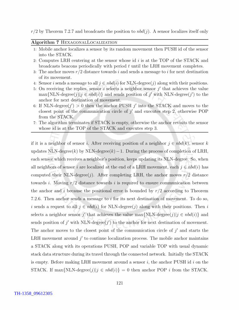
r/2 by Theorem 7.2.7 and broadcasts the position to nbd(j). A sensor localizes itself only
Algorithm 7 HexagonalLocalization
1: Mobile anchor localizes a sensor by its random movement then PUSH id of the sensorinto the STACK.
2: Computes LRH centering at the sensor whose id i is at the TOP of the STACK andbroadcasts beacons periodically with period t until the LRH movement completes.
3: The anchor moves r/2 distance towards i and sends a message to i for next destinationof its movement.
4: Sensor i sends a message to all j ∈ nbd(i) for NLN-degree(j) along with their positions.5: On receiving the replies, sensor i selects a neighbor sensor j′ that achieves the value
max{NLN-degree(j)|j ∈ nbd(i)} and sends position of j′ with NLN-degree(j′) to theanchor for next destination of movement.
6: If NLN-degree(j′) > 0 then the anchor PUSH j′ into the STACK and moves to theclosest point of the communication circle of j′ and executes step 2, otherwise POPfrom the STACK.
7: The algorithm terminates if STACK is empty, otherwise the anchor revisits the sensorwhose id is at the TOP of the STACK and executes step 3.
if it is a neighbor of sensor i. After receiving position of a neighbor j ∈ nbd(k), sensor k
updates NLN-degree(k) by NLN-degree(k)−1. During the process of completion of LRH,
each sensor which receives a neighbor’s position, keeps updating its NLN-degree. So, when
all neighbors of sensor i are localized at the end of a LRH movement, each j ∈ nbd(i) has
computed their NLN-degree(j). After completing LRH, the anchor moves r/2 distance
towards i. Moving r/2 distance towards i is required to ensure communication between
the anchor and i because the positional error is bounded by r/2 according to Theorem
7.2.6. Then anchor sends a message to i for its next destination of movement. To do so,
i sends a request to all j ∈ nbd(i) for NLN-degree(j) along with their positions. Then i
selects a neighbor sensor j′ that achieves the value max{NLN-degree(j)|j ∈ nbd(i)} and
sends position of j′ with NLN-degree(j′) to the anchor for next destination of movement.
The anchor moves to the closest point of the communication circle of j′ and starts the
LRH movement around j′ to continue localization process. The mobile anchor maintains
a STACK along with its operations PUSH, POP and variable TOP with usual dynamic
stack data structure during its travel through the connected network. Initially the STACK
is empty. Before making LRH movement around a sensor i, the anchor PUSH id i on the
STACK. If max{NLN-degree(j)|j ∈ nbd(i)} = 0 then anchor POP i from the STACK.
121
TH-1358_09612305
When the STACK becomes empty, the algorithm terminates, otherwise anchor revisits
the communication circle of the sensor i′ (say), which is at the TOP of the STACK and
then sends a message to i′ for its next destination of movement. Mobile anchor decides
its path according to the Algorithm 7 (HexagonalLocalization).
7.3.1 Correctness and complexity analysis
Theorem 7.3.1. Algorithm 7 ensures localization of all sensors in a connected network.
Proof. We prove correctness of the algorithm by method of contradiction. Let us assume
that one sensor i is not localized but the algorithm terminates, i.e., the STACK becomes
empty. Since all sensors are in a connected network, then there exist at least one sensor
j, which is a neighbor of i and is localized. According to the algorithm, j localizes itself
by marking beacon points on a LRH movement of the anchor around one of its neighbors
k. At this moment k is at the TOP of the STACK. As i is not localized, j would send non
zero NLN-degree(j) and its position to k. Since other sensors are localized, NLN-degree(j)
is the maximum among those received by k. Hence k should send the position of j to the
anchor for the next destination of movement according to Algorithm 7. Whenever anchor
visits j and makes LRH movements, i becomes localized. So k cannot be popped without
pushing j which implies localization of i. Hence k is in the STACK until i is localized.
It contradicts our assumption that the STACK is empty but i is not localized. Hence
proved.
Theorem 7.3.2. The time complexity of Algorithm 7 is O(|V |+ |E|).
Proof. To analyze complexity of Algorithm 7, we calculate maximum travel distance of
the mobile anchor to localize all sensors in any connected graph G = (V,E) topology
in absence of radio irregularity. Here V and E are the set of vertices corresponding to
the sensors and the set of edges of G respectively. If degree of the graph decreases then
the anchor needs to make more LRH movements. The line graph achieves lowest degree
among connected graphs and hence the anchor attends maximum LRH movements to
localize all sensors. In the worst case, for a line graph our algorithm matches with DFS
visit of G. In this case anchor has to make LRH movement around |V | − 1 sensors if it
122
TH-1358_09612305
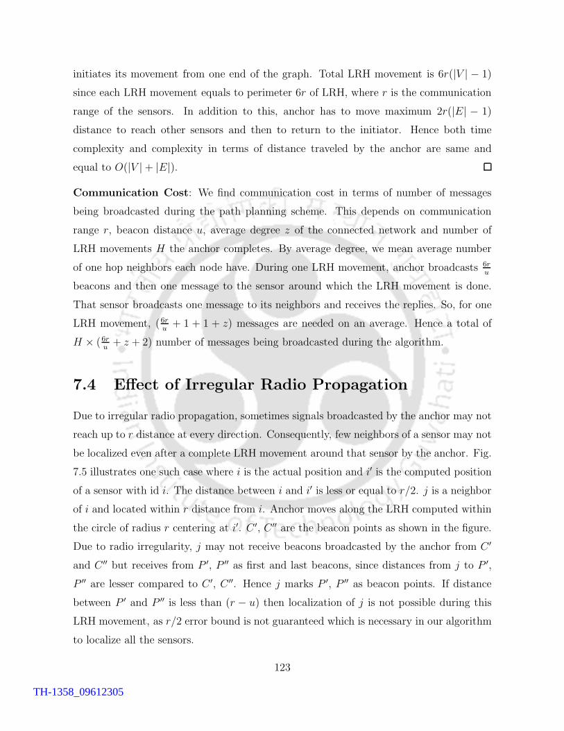
initiates its movement from one end of the graph. Total LRH movement is 6r(|V | − 1)
since each LRH movement equals to perimeter 6r of LRH, where r is the communication
range of the sensors. In addition to this, anchor has to move maximum 2r(|E| − 1)
distance to reach other sensors and then to return to the initiator. Hence both time
complexity and complexity in terms of distance traveled by the anchor are same and
equal to O(|V |+ |E|).
Communication Cost: We find communication cost in terms of number of messages
being broadcasted during the path planning scheme. This depends on communication
range r, beacon distance u, average degree z of the connected network and number of
LRH movements H the anchor completes. By average degree, we mean average number
of one hop neighbors each node have. During one LRH movement, anchor broadcasts 6ru
beacons and then one message to the sensor around which the LRH movement is done.
That sensor broadcasts one message to its neighbors and receives the replies. So, for one
LRH movement, (6ru+ 1 + 1 + z) messages are needed on an average. Hence a total of
H × (6ru+ z + 2) number of messages being broadcasted during the algorithm.
7.4 Effect of Irregular Radio Propagation
Due to irregular radio propagation, sometimes signals broadcasted by the anchor may not
reach up to r distance at every direction. Consequently, few neighbors of a sensor may not
be localized even after a complete LRH movement around that sensor by the anchor. Fig.
7.5 illustrates one such case where i is the actual position and i′ is the computed position
of a sensor with id i. The distance between i and i′ is less or equal to r/2. j is a neighbor
of i and located within r distance from i. Anchor moves along the LRH computed within
the circle of radius r centering at i′. C ′, C ′′ are the beacon points as shown in the figure.
Due to radio irregularity, j may not receive beacons broadcasted by the anchor from C ′
and C ′′ but receives from P ′, P ′′ as first and last beacons, since distances from j to P ′,
P ′′ are lesser compared to C ′, C ′′. Hence j marks P ′, P ′′ as beacon points. If distance
between P ′ and P ′′ is less than (r − u) then localization of j is not possible during this
LRH movement, as r/2 error bound is not guaranteed which is necessary in our algorithm
to localize all the sensors.
123
TH-1358_09612305
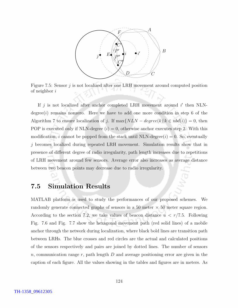
C ′
C ′′
A
B
CD
E
F
P ′′P ′
i i′j
Figure 7.5: Sensor j is not localized after one LRH movement around computed positionof neighbor i
If j is not localized after anchor completed LRH movement around i′ then NLN-
degree(i) remains nonzero. Here we have to add one more condition in step 6 of the
Algorithm 7 to ensure localization of j. If max{NLN − degree(k)|k ∈ nbd(i)} = 0, then
POP is executed only if NLN-degree (i) = 0, otherwise anchor executes step 2. With this
modification, i cannot be popped from the stack until NLN-degree(i) = 0. So, eventually
j becomes localized during repeated LRH movement. Simulation results show that in
presence of different degree of radio irregularity, path length increases due to repetitions
of LRH movement around few sensors. Average error also increases as average distance
between two beacon points may decrease due to radio irregularity.
7.5 Simulation Results
MATLAB platform is used to study the performances of our proposed schemes. We
randomly generate connected graphs of sensors in a 50 meter × 50 meter square region.
According to the section 7.2, we take values of beacon distance u < r/7.5. Following
Fig. 7.6 and Fig. 7.7 show the hexagonal movement path (red solid lines) of a mobile
anchor through the network during localization, where black bold lines are transition path
between LRHs. The blue crosses and red circles are the actual and calculated positions
of the sensors respectively and pairs are joined by dotted lines. The number of sensors
n, communication range r, path length D and average positioning error are given in the
caption of each figure. All the values showing in the tables and figures are in meters. As
124
TH-1358_09612305
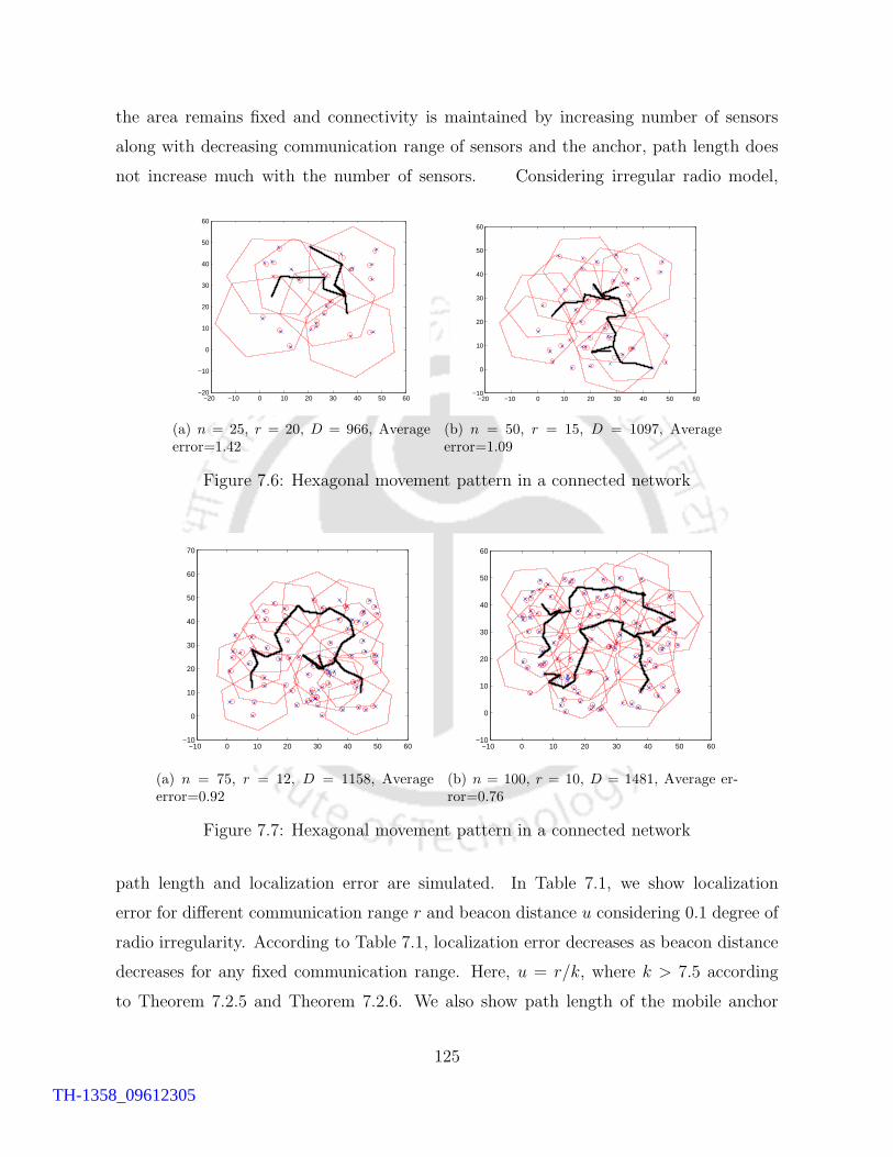
the area remains fixed and connectivity is maintained by increasing number of sensors
along with decreasing communication range of sensors and the anchor, path length does
not increase much with the number of sensors. Considering irregular radio model,
−20 −10 0 10 20 30 40 50 60−20
−10
0
10
20
30
40
50
60
(a) n = 25, r = 20, D = 966, Averageerror=1.42
−20 −10 0 10 20 30 40 50 60−10
0
10
20
30
40
50
60
(b) n = 50, r = 15, D = 1097, Averageerror=1.09
Figure 7.6: Hexagonal movement pattern in a connected network
−10 0 10 20 30 40 50 60−10
0
10
20
30
40
50
60
70
(a) n = 75, r = 12, D = 1158, Averageerror=0.92
−10 0 10 20 30 40 50 60−10
0
10
20
30
40
50
60
(b) n = 100, r = 10, D = 1481, Average er-ror=0.76
Figure 7.7: Hexagonal movement pattern in a connected network
path length and localization error are simulated. In Table 7.1, we show localization
error for different communication range r and beacon distance u considering 0.1 degree of
radio irregularity. According to Table 7.1, localization error decreases as beacon distance
decreases for any fixed communication range. Here, u = r/k, where k > 7.5 according
to Theorem 7.2.5 and Theorem 7.2.6. We also show path length of the mobile anchor
125
TH-1358_09612305
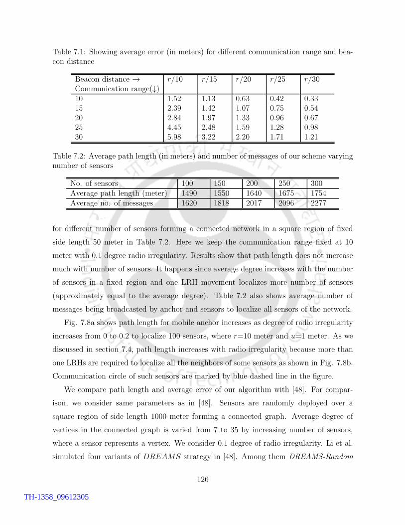
Table 7.1: Showing average error (in meters) for different communication range and bea-con distance
Beacon distance → r/10 r/15 r/20 r/25 r/30Communication range(↓)10 1.52 1.13 0.63 0.42 0.3315 2.39 1.42 1.07 0.75 0.5420 2.84 1.97 1.33 0.96 0.6725 4.45 2.48 1.59 1.28 0.9830 5.98 3.22 2.20 1.71 1.21
Table 7.2: Average path length (in meters) and number of messages of our scheme varyingnumber of sensors
No. of sensors 100 150 200 250 300Average path length (meter) 1490 1550 1640 1675 1754Average no. of messages 1620 1818 2017 2096 2277
for different number of sensors forming a connected network in a square region of fixed
side length 50 meter in Table 7.2. Here we keep the communication range fixed at 10
meter with 0.1 degree radio irregularity. Results show that path length does not increase
much with number of sensors. It happens since average degree increases with the number
of sensors in a fixed region and one LRH movement localizes more number of sensors
(approximately equal to the average degree). Table 7.2 also shows average number of
messages being broadcasted by anchor and sensors to localize all sensors of the network.
Fig. 7.8a shows path length for mobile anchor increases as degree of radio irregularity
increases from 0 to 0.2 to localize 100 sensors, where r=10 meter and u=1 meter. As we
discussed in section 7.4, path length increases with radio irregularity because more than
one LRHs are required to localize all the neighbors of some sensors as shown in Fig. 7.8b.
Communication circle of such sensors are marked by blue dashed line in the figure.
We compare path length and average error of our algorithm with [48]. For compar-
ison, we consider same parameters as in [48]. Sensors are randomly deployed over a
square region of side length 1000 meter forming a connected graph. Average degree of
vertices in the connected graph is varied from 7 to 35 by increasing number of sensors,
where a sensor represents a vertex. We consider 0.1 degree of radio irregularity. Li et al.
simulated four variants of DREAMS strategy in [48]. Among them DREAMS-Random
126
TH-1358_09612305
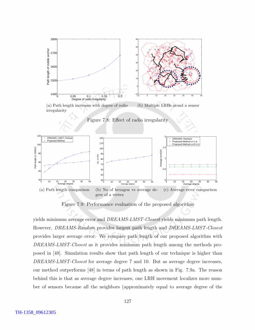
0 0.05 0.1 0.15 0.21400
1500
1600
1700
1800
Degree of radio irregularity
Pat
h le
ngth
of m
obile
anc
hor
(a) Path length increases with degree of redioirregularity
−10 0 10 20 30 40 50 60−10
0
10
20
30
40
50
60
(b) Multiple LRHs arond a sensor
Figure 7.8: Effect of radio irregularity
5 10 15 20 25 30 3520
40
60
80
100
120
Average degree
Pat
h le
ngth
(x
1000
m)
DREAMS−LMST−ClosestProposed Method
(a) Path length comparison
5 10 15 20 25 30 3540
50
60
70
80
90
100
110
120
Average degree
No.
of L
RH
(b) No of hexagon vs average de-gree of a vertex
5 10 15 20 25 30 350
0.5
1
1.5
2
Average degree
Ave
rage
err
or(m
)
DREAMS−RandomProposed Method u=1 mProposed Method u=0.5 m
(c) Average error comparison
Figure 7.9: Performance evaluation of the proposed algorithm
yields minimum average error and DREAMS-LMST-Closest yields minimum path length.
However, DREAMS-Random provides largest path length and DREAMS-LMST-Closest
provides larger average error. We compare path length of our proposed algorithm with
DREAMS-LMST-Closest as it provides minimum path length among the methods pro-
posed in [48]. Simulation results show that path length of our technique is higher than
DREAMS-LMST-Closest for average degree 7 and 10. But as average degree increases,
our method outperforms [48] in terms of path length as shown in Fig. 7.9a. The reason
behind this is that as average degree increases, one LRH movement localizes more num-
ber of sensors because all the neighbors (approximately equal to average degree of the
127
TH-1358_09612305
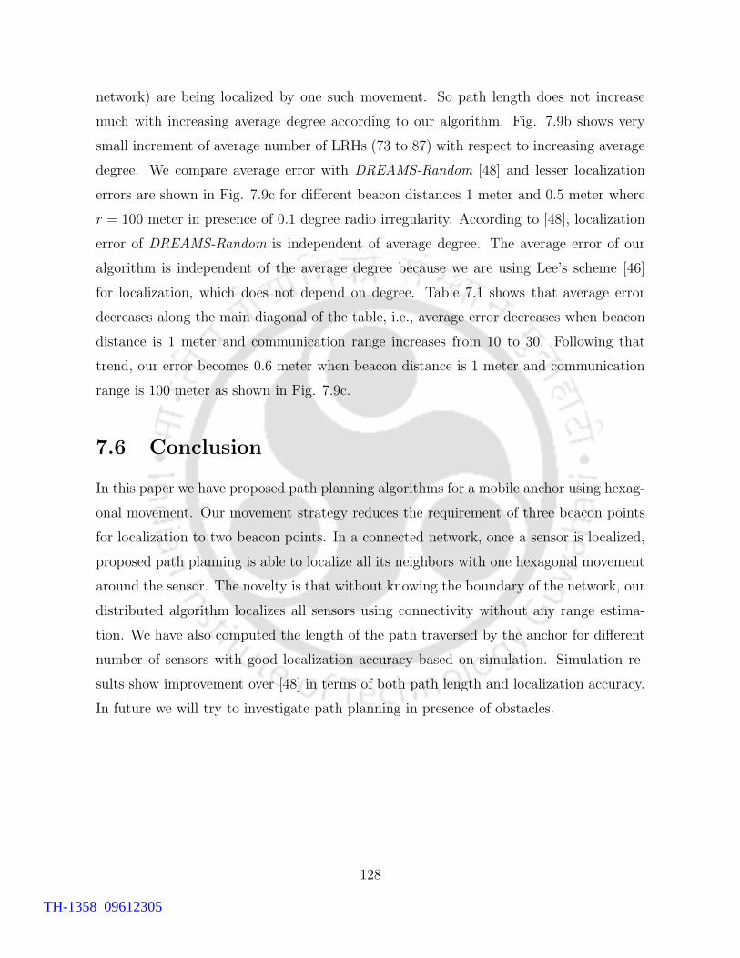
network) are being localized by one such movement. So path length does not increase
much with increasing average degree according to our algorithm. Fig. 7.9b shows very
small increment of average number of LRHs (73 to 87) with respect to increasing average
degree. We compare average error with DREAMS-Random [48] and lesser localization
errors are shown in Fig. 7.9c for different beacon distances 1 meter and 0.5 meter where
r = 100 meter in presence of 0.1 degree radio irregularity. According to [48], localization
error of DREAMS-Random is independent of average degree. The average error of our
algorithm is independent of the average degree because we are using Lee’s scheme [46]
for localization, which does not depend on degree. Table 7.1 shows that average error
decreases along the main diagonal of the table, i.e., average error decreases when beacon
distance is 1 meter and communication range increases from 10 to 30. Following that
trend, our error becomes 0.6 meter when beacon distance is 1 meter and communication
range is 100 meter as shown in Fig. 7.9c.
7.6 Conclusion
In this paper we have proposed path planning algorithms for a mobile anchor using hexag-
onal movement. Our movement strategy reduces the requirement of three beacon points
for localization to two beacon points. In a connected network, once a sensor is localized,
proposed path planning is able to localize all its neighbors with one hexagonal movement
around the sensor. The novelty is that without knowing the boundary of the network, our
distributed algorithm localizes all sensors using connectivity without any range estima-
tion. We have also computed the length of the path traversed by the anchor for different
number of sensors with good localization accuracy based on simulation. Simulation re-
sults show improvement over [48] in terms of both path length and localization accuracy.
In future we will try to investigate path planning in presence of obstacles.
128
TH-1358_09612305
Chapter 8
Path Planning for Mobile Anchor in
Rectangular Regions
8.1 Introduction
In this chapter we consider the path planning problem for a mobile anchor where the region
of interest is known beforehand like indoor networks. Our aim is to propose a movement
strategy in a bounded region for a mobile anchor such that it can use existing range-
free localization schemes which yields better accuracy while reducing the path length. In
our strategy, only boundary information is used to localize all the sensors irrespective of
deployment and underlying network topology. Comparison with existing literature shows
reduction in path length along with good positioning accuracy.
8.1.1 Our contribution
We propose a movement strategy for mobile anchor which localizes all the sensors ly-
ing within the region using hexagonal tiling to cover a rectangular region with known
boundary information. Theoretically we show that the length of the path traversed by
the anchor is lesser in the proposed strategy compared to other existing path planning
methods [25, 34, 37, 59] for covering a rectangular region. Results show 7.35% to 27.74%
improvement of our scheme over different schemes in terms of path length. Good local-
ization accuracy is also observed in simulation.
129
TH-1358_09612305
The organization of the remaining part of the work is as follows. The theoretical
results of our proposed path planning in a rectangular region are explained in section 8.2.
The simulation results are presented in section 8.3, along with performance comparison
with existing approaches. Finally we conclude in section 8.4.
8.2 Path Planning for Rectangular Region
The mobile anchor broadcasts beacon with its position information after every t time
interval. We may use the term ‘anchor’ instead ‘mobile anchor’ in the rest of this chapter.
Definitions of beacon distance and beacon points are same as given in chapter 7. Here
also we use localization scheme [46]. How this scheme works and our hexagonal movement
strategy reduces the requirement of three beacon points to two beacon points are already
discussed in section 7.2 of chapter 7.
In this section we discuss path planning for a mobile anchor which covers a given rect-
angular region to ensure localization of all sensors deployed in that region. Let ABCDEF
be a regular hexagon with side length r and center O as shown in Fig. 8.1a. If commu-
nication circle of a sensor touches the hexagon then we say that the sensor is within the
coverage area of the hexagon. Obviously the area inside the hexagon is a part of the cov-
erage area. As shown in Fig. 8.1a, A′B′C ′D′E ′F ′ is a regular hexagon with side 2r and
center O. The communication circles of the sensors located at the vertices of the larger
hexagon touch the smaller hexagon at one vertex. Communication circle of any sensor
which lies within or on the larger hexagon except at the vertices, intersects the smaller
hexagon at at least two points. So A′B′C ′D′E ′F ′ forms a coverage area of ABCDEF .
Let the anchor moves along ABCDEF broadcasting beacons periodically with time
period t. To localize itself following the scheme [46], each sensor should mark at least two
beacon points on ABCDEF . To ensure marking of two beacon points, we reduce the
coverage area by reducing the hexagon A′B′C ′D′E ′F ′ to A′′B′′C ′′D′′E ′′F ′′ with side 2r−X
as shown in Fig. 8.1b. Now, we have to find a suitable value of X such that all sensors
located inside A′′B′′C ′′D′′E ′′F ′′ can be localized. As the vertices of A′′B′′C ′′D′′E ′′F ′′ are
the furthest points from ABCDEF , so if we find X in such a way that a sensor which
lies at any vertex of A′′B′′C ′′D′′E ′′F ′′, marks at least two beacon points, then so does
130
TH-1358_09612305
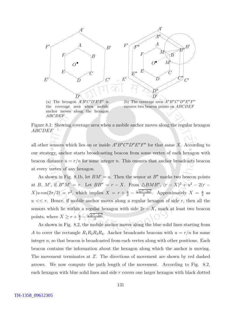
O
A
B
C
D
E
F
A′
B′
C ′
D′
E ′
F ′
(a) The hexagon A′B′C′D′E′F ′ isthe coverage area when mobileanchor moves along the hexagonABCDEF
O
A
M
M ′B
C
D
E
F
A′
B′
C ′
D′
E ′
F ′
A′′
B′′
C ′′
D′′
E ′′
F ′′
(b) The coverage area A′′B′′C′′D′′E′′F ′′
ensures two beacon points on ABCDEF
Figure 8.1: Showing coverage area when a mobile anchor moves along the regular hexagonABCDEF
all other sensors which lies on or inside A′′B′′C ′′D′′E ′′F ′′ for that same X . According to
our strategy, anchor starts broadcasting beacon from some vertex of each hexagon with
beacon distance u = r/n for some integer n. This ensures that anchor broadcasts beacon
at every vertex of any hexagon.
As shown in Fig. 8.1b, let BM ′ = u. Then the sensor at B′′ marks two beacon points
at B, M ′, if B′′M ′ = r. Let BB′′ = r − X . From 4BMB′′, (r − X)2 + u2 − 2(r −X)u cos(2π/3) = r2, which implies X = r + u
2−
√4r2−3u2
2. Approximately X = u
2as
u << r. Hence, if mobile anchor moves along a regular hexagon of side r, then all the
sensors which lie within a regular hexagon with side 2r − X , mark at least two beacon
points, where X ≥ r + u2−
√4r2−3u2
2.
As shown in Fig. 8.2, the mobile anchor moves along the blue solid lines starting from
A to cover the rectangle R1R2R3R4. Anchor broadcasts beacons with u = r/n for some
integer n, so that beacon is broadcasted from each vertex along with other positions. Each
beacon contains the information about the hexagon along which the anchor is moving.
The movement terminates at Z. The directions of movement are shown by red dashed
arrows. We now compute the path length of the movement. According to Fig. 8.2,
each hexagon with blue solid lines and side r covers one larger hexagon with black dotted
131
TH-1358_09612305

Z
RR
R R
A
H
H H
H
1
1
2
2
3
3
4
4
Figure 8.2: Showing path planning to cover a rectangular region R1R2R3R4
lines whose width is equal to H2H4 =√
(2r −X)2 + (2r −X)2 − 2(2r −X)2 cos(2π/3) =√3(2r − X). If L is the width of the rectangle, then the number of hexagon in a row
would be⌈
L√3(2r−X)
⌉
. Two rows of hexagon cover an area with height equal to H1H3 =
H1H2 +H2H3 = 3(2r −X). If L is the height of the rectangle, then the number of rows
of hexagon would be⌈
L3(2r−X)/2
⌉
. Then total number of hexagon with side r required to
cover a L × L rectangle is⌈
L√3(2r−X)
⌉ ⌈
2L3(2r−X)
⌉
. Total path length required to reach all
the hexagons in a row by moving from one hexagon to another hexagon is at most L.
So, total distance traversed to connect the hexagons for all rows is equal to L⌈
2L3(2r−X)
⌉
.
Total path length required to reach all the rows by moving from one row to another row
is at most L again. In each pair of consecutive rows, an extra hexagon is needed i.e., an
extra 3r movement is required in each row on an average. So, total path traversed to
cover L× L rectangle is equal to
DHexagon =⌈
L√3(2r−X)
⌉ ⌈
2L3(2r−X)
⌉
6r + L⌈
2L3(2r−X)
⌉
+ 3r⌈
2L3(2r−X)
⌉
+ L.
Number of beacons transmitted by the mobile anchor throughout the traversal is
equal to number of hexagons multiplied by 6r/u since during moving on each hexagon
6r/u number of beacons are transmitted.
132
TH-1358_09612305
8.2.1 Comparison with existing schemes
Table 8.1: Coefficients of higher order term L2/r in the expressions of different schemesincluding proposed scheme (DHexagon)
DHexagon DChia DScan DDScan DHilbert DS−curves DCircles DLMAT
1√3
(
2k2k−1
)(
2k2k−1 +
1√3
)
kk−1
kk−1
kk−1
kk−1
π3
(
kk−1
)
π2
(
kk−1
)
2√3
Theoretical comparison with existing schemes [25, 34, 37, 59] in terms of path length
of mobile anchor is presented in this section. Let L be the length of the sides of a square
region and r be the communication range of sensors and anchor. To normalize all the
expressions of path length given in [59], we take X = r/k for some integer k > 1. We
denote path length of path planning of mobile anchor proposed in [59] by DChia. Path
lengths of mobile anchor in different schemes in [37] are denoted by DScan, DDScan and
DHilbert. Path lengths of mobile anchor in different schemes in [34] are denoted by DCircles
and DS−curves. DLMAT is the path length of the scheme proposed by [25]. We denote the
path length of mobile anchor of our proposed scheme by DHexagon. Expressions of path
lengths of different schemes are given below.
DChia = (L+ 2r)(⌈(
L+2rr−r/k
)⌉
+ 1)
+ (r − r/k)⌈(
L+2rr−r/k
)⌉
DScan =⌈(
Lr−r/k
+ 2)⌉
L
DDScan = 2(⌈(
L−r2(r−r/k)
+ 2)⌉
L− r)
DHilbert =⌈(
L+rr−r/k
)⌉2
(r − r/k)
DS−curves =[(
L3(r−r/k)/2
+ 1)
L2π]
+ L+ rπ/2
DCircles = N2π(r − r/k)+L, where N = L/√2−r
r−r/k
Expression of DCircles is modified in such a way that it can also cover the corner points
of the rectangle.
According to [25],
DLMAT = 2√3L(⌈
Lr
⌉)
+ L+ r√3
The path length for our proposed scheme is
DHexagon =⌈
L√3(2r−r/k)
⌉ ⌈
2L3(2r−r/k)
⌉
6r + L⌈
2L3(2r−r/k)
⌉
+ 3r⌈
2L3(2r−r/k)
⌉
+ L.
133
TH-1358_09612305
In all the above expressions, the highest order term is L2/r. So, we compare the
coefficients of L2/r as shown in Table 8.1 to decide minimality of path length theoretically.
In DChia, DScan, DDScan and DHilbert, the coefficient of higher order term L2/r is equal to
kk−1
. For DS−curves, the coefficient of L2/r is π3
(
kk−1
)
. The coefficient of L2/r in DCircles
is π2
(
kk−1
)
. The coefficient of L2/r in DHexagon is 1√3
(
2k2k−1
)
(
2k2k−1
+ 1√3
)
. We show that
coefficient of L2/r in DHexagon is lesser than all the above mentioned coefficients for all
k. Among the existing path planning schemes Circles in [34] does best in terms of path
length to cover a circular region. But for a square region, larger circles are needed to cover
the corners of the square, which increases path length and makes Circles an inefficient
strategy for covering a square. Since π2
(
kk−1
)
> π3
(
kk−1
)
> kk−1
for all k > 1, so if we can
show kk−1
> 1√3
(
2k2k−1
)
(
2k2k−1
+ 1√3
)
for all k, then we can claim the minimality of path
length of our scheme as the coefficient of the highest order term L2/r of our scheme is least
among the aforesaid schemes. One can easily verify that kk−1
> 1√3
(
2k2k−1
)
(
2k2k−1
+ 1√3
)
for 2 ≤ k ≤ 9. Again, for all k ≥ 10, 1√3
(
2k2k−1
)
(
2k2k−1
+ 1√3
)
< 1 but kk−1
> 1. Hence for
any r, there exists L such that path length of DHexagon is minimum. Considering LMAT
in [25], coefficient of L2/r in DHexagon beats DLMAT for all k ≥ 5. So, for any r, there
exists L such that path length of DHexagon is lesser compared to DLMAT .
8.3 Simulation Results
MATLAB platform is used to study the performances of our proposed schemes. We
evaluate path length of the proposed scheme for a bounded region for X = r/20 and
compared with existing range based and range free schemes. The value of communication
range r = 10 meter and square region with side length L = 200 meter. Results are shown
in Table 8.2. We show the percentages of improvement of our scheme over various schemes
compared to path length in Table 8.3 for r = 10 and X = r/20. Results show 7.35% to
27.74% improvement over different schemes. Values of average localization error of our
scheme are shown in Table 8.4 varying communication ranges r and beacon distance u.
We take X = u in Table 8.4. Here also, localization error decreases as beacon distance
decreases for any fixed communication range.
Path planning schemes in [25, 37] localize sensors using range-based methods. Hence
134
TH-1358_09612305

Table 8.2: Comparison of path length (in meter) of our scheme (DHexagon) with existingschemes
DHexagon DChia DScan DDScan DHilbert DCircles DS−curves DLMAT
4271 5728 4610 4780 4620 5911 4939 4836
Table 8.3: Percentage (%) of improvement of our scheme in terms of path length comparedto existing schemes
Existing schemes DChia DScan DDScan DHilbert DCircles DS−curves DLMAT
% of improvement ofour schemecompared to theexisting schemes interms of path length
25.43% 7.35% 10.64% 7.55% 27.74% 13.52% 13.22%
yields better accuracy than our proposed method as we use range-free method for local-
ization. However we have better results in terms of path length. In [59], Chia-Ho-Ou et
al. produces better localization accuracy with average error 0.5 meter when communi-
cation range is equal to 20 meter and beacon distance is 1 meter, whereas under same
condition our average error is 1.6 meter. But our scheme outperforms in terms of path
length compared to [59].
Table 8.4: Showing average error (in meter) for different communication range and beacondistance
Beacon distance → r/10 r/15 r/20 r/25 r/30Communication range(↓)10 1.59 1.17 0.78 0.57 0.4615 2.75 1.58 1.22 0.98 0.8520 2.93 1.95 1.61 1.17 0.8925 4.28 2.47 1.61 1.19 0.9930 4.94 2.65 1.72 1.36 1.11
135
TH-1358_09612305

8.4 Conclusion
With our proposed path planning strategy, it is possible to localize all sensors in a rect-
angular region with known boundary. We have compared path length of our proposed
movement strategy for rectangular region theoretically with existing literature to show
better performance. Simulation results show 7.35% to 27.74% improvement of our path
planning strategy over existing strategies in terms of path length of mobile anchor for
rectangular region. In future we will try to investigate path planning in presence of
obstacles.
136
TH-1358_09612305
Chapter 9
Conclusion
At the beginning of the thesis we have proposed two deterministic range-based localiza-
tion algorithms for static sensors in presence of NLOS signals using static anchors. The
algorithm (FindPosition(φ, w)) finds position of a static sensor based on receiving two
reflected signals from an anchor. If a sensor receives signals from different anchors, then
communication among anchors are required. The proposed technique does not need to
know the positions of those reflectors. The algorithm produces actual position of a sensor
if there are no range measurement errors. In presence of measurement errors, the algo-
rithm returns approximate position of the sensor. Simulation results show better accuracy
of our scheme compared to existing works in presence of measurement errors. The strong
point of our approach is that our algorithm works in a sparse network since only two re-
flected signals from an anchor are sufficient for finding position of a sensor. Another good
aspect of our algorithm is that the positioning error does not increase significantly with
significant increment of distance measurement error. The weak aspect of this approach
is, however, that we have put restriction on NLOS signals. We have also considered a
three dimensional space and got similar results for exact positioning of sensors. We have
proved that with accurate range measurements, anchor can detect presence of misbehav-
ing sensor under certain conditions. However, further studies are needed in this direction
for detecting misbehaving sensors in presence of measurement errors. To generalize the
above problem, we have proposed a localization algorithm (LocalizeSensor) consider-
ing multiple-bound signals. Our algorithm provides a circle within which the sensor is
137
TH-1358_09612305
bound to reside for each received unknown-bound signal. Theoretically we have shown
that radius of this circle is lesser than the distance traveled by the signal. Hence our
algorithm outperforms trilateration in terms of positional accuracy.
Two deterministic range-free localization algorithms (LWCD and LCD) for mobile
sensors using static anchors have been proposed. In presence of obstacles we have modified
above algorithms and proposed LWCDPO and LPO respectively. The algorithms work
under irregular radio model. LWCD and LWCDPO assume that there is no change of
direction of the mobile sensor during localization. We have given bounds on localization
error of LWCD for a given communication range and beacon distance. LWCD is able
to localize sensors within any predetermined error bound by fixing appropriate beacon
distance for any given communication range. Using our technique a mobile sensor can
further reduce localization error whenever it passes through the communication circle
of different anchors by repeated calculation of the approximate line of movement. We
have shown that the upper bound of the localization error of LWCDPO remains same
as LCD. Simulation results show that in our approach, average error is very less than
the maximum possible error and the algorithm outperforms over the existing approaches
in terms of positional accuracy. LCD and LPO give a general solution where mobile
sensor can change direction of movement within communication circle of an anchor. LPO
uses two different signal strength of static anchors effectively to select appropriate beacon
points in presence of obstacles. Better positioning accuracy is observed in simulation for
LCD and LPO compared to existing works.
A mobile anchor is equivalent to many static anchors for localizing sensors in a network.
Suitable movement strategies help reducing travel path and provide better accuracy if a
good localization scheme can be used while following the path planning algorithm. A
distributed range-free path planning algorithm (HexagonalLocalization) for mobile
anchors is proposed to localize static sensors in a connected network. Proposed algorithm
localizes all sensors using connectivity without any knowledge of the deployment area.
Simulation results show improvement over existing works in terms of both path length
and localization accuracy. Another movement strategy for mobile anchors is proposed to
localize sensors in a rectangular region with known boundary. Path length of our proposed
movement strategy is lesser compared to existing literatures. The basic structure of both
138
TH-1358_09612305

the proposed strategies is hexagonal movement. The hexagonal movement reduces the
usual requirement of three beacon points for localization to two beacon points which helps
to improve path length. Summary of the thesis work is represented in tabular form in the
Table 9.1.
Table 9.1: Tabular representation of the thesis work
Algorithm Anchor Sensor Type Assumptions Techniq-ue used
Errorbound
Min.No. ofsignals/beaconpoints
1 Static Static Rangebased
At most one re-flection
AOA,TOA
No One
2 Static Static Rangebased
Known upperbound on num-ber of reflections
AOA,TOA,RSSI
No One
3, 4 Static Mobile Rangefree
Direction un-changed duringlocalization
Beaconpointselection
Yes Four
5, 6 Static Mobile Rangefree
Direction maychange duringlocalization
Beaconpointselection
No Two
7 Mobile Static Rangefree
Connected net-work
Beaconpoint onLRH
Yes Two
Rectangularregion
Mobile Static Rangefree
Known bound-ary
Beaconpoint onHexagon
Yes Two
In future we can think of a more practical approach towards multiple-bound NLOS
problem by considering measurement errors. The mobile sensor localization problem can
be extended by considering the case where mobile sensor changes direction after passing
through a communication circle of some anchor and before entering in the communication
circle of some other anchor. We have not considered presence of obstacle in any of the
path planning problems which can be an important extension. Apart from these, we can
look into anchor-free localization problems as well.
139
TH-1358_09612305

TH-1358_09612305
Bibliography
[1] Galstyan A., Krishnamachari B., Lerman K., and Pattem S. Distributed online local-
ization in sensor networks using a moving target. In Third International Symposium
on Information Processing in Sensor Networks, 2004. IPSN 2004, pages 61–70, 2004.
[2] Hady S. AbdelSalam and Stephan Olariu. Hexnet: Hexagon-based localization tech-
nique for wireless sensor networks. In Seventh Annual IEEE International Conference
on Pervasive Computing and Communications - Workshops (PerCom Workshops
2009), 9-13 March 2009, Galveston, TX, USA, pages 1–6, 2009.
[3] Hady S. AbdelSalam, Stephan Olariu, and Syed R. Rizvi. Tiling-based localiza-
tion scheme for sensor networks using a single beacon. In Proceedings of the Global
Communications Conference, 2008. GLOBECOM 2008, New Orleans, LA, USA, 30
November - 4 December 2008, pages 790–794, 2008.
[4] Aylin Aksu and Prashant Krisnamurthy. Sub-area localization: A simple calibration
free approach. In Proc. of MSWIM’10, 2010.
[5] Shafagh Alikhani, Thomas Kunz, and Marc St-Hilaire. iCCA-MAP versus MCL and
dual MCL: Comparison of mobile node localization algorithms. In ADHOC-NOW,
pages 163–176, 2010.
[6] Waleed Ammar, Ahmed ElDawy, and Moustafa Youssef. Secure localization in wire-
less sensor networks: A survey. CoRR, abs/1004.3164, 2010.
[7] Aline Baggio and Koen Langendoen. Monte-carlo localization for mobile wireless
sensor networks. In MSN, pages 317–328, 2006.
141
TH-1358_09612305

[8] Kostas E. Bekris, Antonis A. Argyros, and Lydia E. Kavraki. Angle-based methods
for mobile robot navigation: Reaching the entire plane. In ICRA, pages 2373–2378,
2004.
[9] Nirupama Bulusu, John S. Heidemann, and Deborah Estrin. Gps-less low-cost out-
door localization for very small devices. IEEE Personal Commun., 7(5):28–34, 2000.
[10] Srdjan Capkun and Jean-Pierre Hubaux. Secure positioning of wireless devices with
application to sensor networks. In INFOCOM, pages 1917–1928, 2005.
[11] Alberto Cerpa, Jeremy Elson, Deborah Estrin, Lewis Girod, Mic hael Hamilton,
and Jerry Zhao. Habitat monitoring: application driver for wireless communications
technology. Computer Communication Review, 31(2-Supplement):20–41, 2001.
[12] Yiu-Tong Chan, Wing-Yue Tsui, Hing-Cheung So, and Pak-Chung Ching. Time-
of-arrival based localization under nlos conditions. IEEE T. Vehicular Technology,
55(1):17–24, 2006.
[13] C. T. Chang, C. Y. Chang, and C. Y. Lin. Anchor-guiding mechanism for beacon-
assisted localization in wireless sensor networks. IEEE SENSORS JOURNAL,
12(5):1098–1111, 2012.
[14] Hongyang Chen, Gang Wang, Zizhuo Wang, Hing-Cheung So, and H Vincent Poor.
Non-line-of-sight node localization based on semi definite programming in wireless
sensor networks. IEEE Transaction on Wireless Communication, 11(1):108–116,
2012.
[15] X. Cheng, A. Thaeler, G. Xue, and D. Chen. TPS: A time-based positioning scheme
for outdoor wireless sensor networks. In INFOCOM, 2004.
[16] Xiuzhen Cheng, Xiao Huang, and Ding-Zhu Du. Ad-hoc wireless networking. Springer
Verlag, 2004.
[17] Chia-Ho-Ou. A localization scheme for wireless sensor networks using mobile anchors
with directional antennas. Sensors Journal, IEEE, 11(7):1607–1616, 2011.
142
TH-1358_09612305
[18] Karthik Dantu, Mohammad H. Rahimi, Hardik Shah, Sandeep Babel, Amit Dhari-
wal, and Gaurav S. Sukhatme. Robomote: enabling mobility in sensor networks. In
IPSN, pages 404–409, 2005.
[19] Suprakash Datta, Chris Klinowski, Masoomeh Rudafshani, and Shaker Khaleque.
Distributed localization in static and mobile sensor networks. In WiMob, pages 69–
76, 2006.
[20] Sylvie Delat, Partha Sarathi Mandal, Mariusz A. Rokicki, and Sbastien Tixeuil.
Deterministic secure positioning in wireless sensor networks. Theoretical Computer
Science, 412(35):4471 – 4481, 2011.
[21] Anirvan DuttaGupta, Arijit Bishnu, and Indranil Sengupta. Maximal breach in
wireless sensor networks: Geometric characterization and algorithms. In Miroslaw
Kutylowski, Jacek Cichon, and Przemyslaw Kubiak, editors, Algorithmic Aspects of
Wireless Sensor Networks, Third International Workshop, ALGOSENSORS 2007,
Wroclaw, Poland, July 14, 2007, Revised Selected Papers, volume 4837 of Lecture
Notes in Computer Science, pages 126–137. Springer, 2007.
[22] Z. Ebrahimian and R. A Scholtz. Source localization using reflection omission in the
near-field. In IEEE-ACES Conf. on Applied Comput. Electromagnetics, 2005.
[23] Jonathan Friedman, David Lee, Ilias Tsigkogiannis, Sophia Wong, Dennis Chao,
David Levin, William J. Kaiser, and Mani B. Srivastava. RAGOBOT: A new platform
for wireless mobile sensor networks. In DCOSS, pages 412–412, 2005.
[24] Richard Fuller and Xenofon D. Koutsoukos, editors. Mobile Entity Localization and
Tracking in GPS-less Environnments, Second International Workshop, MELT 2009,
Orlando, FL, USA, September 30, 2009. Proceedings, volume 5801 of Lecture Notes
in Computer Science. Springer, 2009.
[25] Han G., Xu H., Jiang J., Shu L., Hara T., and Nishio S. Path planning using
a mobile anchor node based on trilateration in wireless sensor networks. Wireless
Communications and Mobile Computing, 13(14):1324–1336, 2013.
143
TH-1358_09612305
[26] Lewis Girod and Deborah Estrin. Robust range estimation using acoustic and mul-
timodal sensing. In IROS, pages 1312–1320, 2001.
[27] Guangjie Han, Deokjai Choi, and Wontaek Lim. Reference node placement and
selection algorithm based on trilateration for indoor sensor networks. Wireless Com-
munications and Mobile Computing, 9(8):1017–1027, 2009.
[28] Guangjie Han, Huihui Xu, Trung Q. Duong, Jinfang Jiang, and Takahiro Hara.
Localization algorithms of wireless sensor networks: a survey. Telecommunication
Systems, 52(4):2419–2436, 2013.
[29] Guangjie Han, Chenyu Zhang, Jaime Lloret, Lei Shu, and Joel J. P. C. Rodrigues.
A mobile anchor assisted localization algorithm based on regular hexagon in wireless
sensor networks. The Scientific World Journal, 2014, 2014.
[30] Tian He, Chengdu Huang, Brian M. Blum, John A. Stankovic, and Tarek Abdelzaher.
Range-free localization schemes for large scale sensor networks. In Proc. of 9th Annual
Int. Conf. on Mobile Computing and Networking, MobiCom ’03, pages 81–95, New
York, USA, 2003. ACM.
[31] B. Hofmann-Wellenhof, H. Lichtenegger, and J. Collins. Global Positioning System:
Theory and Practice, 4th edition. Springer Verlag, 1997.
[32] Chen-Chien Hsu, Hsin-Chuan Chen, and Chien-Yu Lai. An improved ultrasonic-
based localization using reflection method. In CAR, pages 437–440, 2009.
[33] Lingxuan Hu and David Evans. Localization for mobile sensor networks. In MOBI-
COM, pages 45–57, 2004.
[34] Rui Huang and Gergely V. Zaruba. Static path planning for mobile beacons to
localize sensor networks. In PerCom Workshops, pages 323–330, 2007.
[35] S. Jauregui-Ortiz, M. Siller, and F. Ramos. Node localization in wsn using trigono-
metric figures. In IEEE Topical Conf. on Wireless Sensors and Sensor Networks
(WiSNet), pages 65 –68, jan. 2011.
144
TH-1358_09612305
[36] Kyunghwi Kim, Byunghyuk Jung, Wonjun Lee, and Ding-Zhu Du. Adaptive
path planning for randomly deployed wireless sensor networks. J. Inf. Sci. Eng.,
27(3):1091–1106, 2011.
[37] Dimitrios Koutsonikolas, Saumitra M. Das, and Y. Charlie Hu. Path planning of
mobile landmarks for localization in wireless sensor networks. Computer Communi-
cations, 30(13):2577–2592, 2007.
[38] Xing-Hong KUANG, Hui-He SHAO, and Rui FENG. A new distributed localization
scheme for wireless sensor networks. Acta Automatica Sinica, 34(3):344 – 348, 2008.
[39] A. V. U. Phani Kumar, Adi Mallikarjuna Reddy V, and D. Janaki Ram. Distributed
collaboration for event detection in wireless sensor networks. In Proceedings of the 3rd
International Workshop on Middleware for Pervasive and Ad-hoc Computing (MPAC
2005), held at the ACM/IFIP/USENIX 6th International Middleware Conference,
November 28 - December 2, 2005, Grenoble, France, pages 1–8, 2005.
[40] Branislav Kusy, Akos Ledeczi, and Xenofon D. Koutsoukos. Tracking mobile nodes
using RF doppler shifts. In SenSys, pages 29–42, 2007.
[41] Branislav Kusy, Janos Sallai, Gyorgy Balogh, Akos Ledeczi, Vladimir A. Pro-
topopescu, Johnny Tolliver, Frank DeNap, and Morey Parang. Radio interferometric
tracking of mobile wireless nodes. In MobiSys, pages 139–151, 2007.
[42] DAI Gui lan;ZHAO Chong-chong;QIU Yan;. A localization scheme based on sphere
for wireless sensor network in 3d. Chinese Journal of Electronics, 36(7):1297, 2008.
[43] Julian Lategahn, Marcel Muller, and Christof Rohrig. TDoA and RSS based extended
kalman filter for indoor person localization. In Proceedings of the 78th IEEE Vehicular
Technology Conference, VTC Fall 2013, Las Vegas, NV, USA, September 2-5, 2013,
pages 1–5, 2013.
[44] Loukas Lazos and Radha Poovendran. Hirloc: high-resolution robust localization
for wireless sensor networks. IEEE Journal on Selected Areas in Communications,
24(2):233–246, 2006.
145
TH-1358_09612305
[45] HyungJune Lee, Martin Wicke, Branislav Kusy, and Leonidas Guibas. Localization of
mobile users using trajectory matching. In Proceedings of the first ACM international
workshop on Mobile entity localization and tracking in GPS-less environments, MELT
’08, pages 123–128, New York, NY, USA, 2008. ACM.
[46] Sangho Lee, Eunchan Kim, Chungsan Kim, and Kiseon Kim. Localization with a
mobile beacon based on geometric constraints in wireless sensor networks. IEEE
Transactions on Wireless Communications, 8(12):5801–5805, 2009.
[47] Hongjun Li, Jianwen Wang, Xun Li, and Hongxu Ma. Real-time path planning of
mobile anchor node in localization for wireless sensor networks. In International
Conference on Information and Automation, 2008. ICIA 2008., pages 384 – 389,
2008.
[48] Xu Li, Nathalie Mitton, Isabelle Simplot-Ryl, and David Simplot-Ryl. Dynamic
beacon mobility scheduling for sensor localization. IEEE Trans. Parallel Distrib.
Syst., 23(8):1439–1452, 2012.
[49] C. H. Liu and D. J. Fang. Propagation. in antenna handbook: Theory, applications,
and design. Van Nostrand Reinhold, Chapter 29:1–56, 1988.
[50] R.C. Luo, O. Chen, and S.H. Pan. Mobile user localization in wireless sensor network
using grey prediction method. In IECON, pages 2689–2685, 2005.
[51] Honglei Miao, Kegen Yu, and M.J. Juntti. Positioning for NLOS propagation: Algo-
rithm derivations and cramer-rao bounds. Vehicular Technology, IEEE Transactions
on, 56(5):2568–2580, Sept 2007.
[52] Sichitiu M.L. and Ramadurai V. Localization of wireless sensor networks with a
mobile beacon. In IEEE International Conference on Mobile Ad-hoc and Sensor
Systems, 2004, pages 174–183, 2004.
[53] Bernd Neuwinger, Ulf Witkowski, and Ulrich Ruckert. Ad-hoc communication and
localization system for mobile robots. volume 5744/2009 of Advances in Robotics,
pages 220–229. Springer-Verlag, 2009.
146
TH-1358_09612305
[54] Dragos Niculescu and B. R. Badrinath. Ad hoc positioning system (APS) using AOA.
In INFOCOM, 2003.
[55] Dragos Niculescu and Badri Nath. DV based positioning in ad hoc networks. Telecom-
munication Systems, 22(1-4):267–280, 2003.
[56] Georg Oberholzer, Philipp Sommer, and Roger Wattenhofer. SpiderBat: Augmenting
wireless sensor networks with distance and angle information. In IPSN, pages 211–
222, 2011.
[57] Tomoaki Ogawa, Shuichi Yoshino, Masashi Shimizu, and Hirohito Suda. A new in-
door location detection method adopting learning algorithms. In PerCom, pages
525–530, 2003.
[58] Chia-Ho Ou. Range-free node localization for mobile wireless sensor networks. In
ISWPC, pages 535–539, 2008.
[59] Chia-Ho Ou. Path planning algorithm for mobile anchor-based localization in wireless
sensor networks. IEEE SENSORS JOURNAL, 13(2):466–475, 2013.
[60] Chia-Ho Ou and Kuo-Feng Ssu. Sensor position determination with flying anchors in
three-dimensional wireless sensor networks. IEEE Trans. Mob. Comput., 7(9):1084–
1097, 2008.
[61] Kaveh Pahlavan, Ferit O. Akgul, Mohammad Heidari, Ahmad Hatami, John M.
Elwell, and Robert D. Tingley. Indoor geolocation in the absence of direct path.
IEEE Wireless Communications, 13(6):50 –58, dec. 2006.
[62] Mayuresh M. Patil, Umesh Shaha, U. B. Desai, and S. N. Merchant. Localization in
wireless sensor networks using three masters. Proc. of IEEE Int. Conf. on Personal
Wireless Commun. (ICPWC’05), pages 384–388, 2005.
[63] Nissanka B. Priyantha, Allen K.L. Miu, Hari Balakrishnan, and Seth Teller. The
cricket compass for context-aware mobile applications. In Proceedings of the 7th
annual international conference on Mobile computing and networking, MobiCom ’01,
pages 1–14, New York, NY, USA, 2001. ACM.
147
TH-1358_09612305
[64] Yihong Qi, Hisashi Kobayashi, and Hirohito Suda. Analysis of wireless geolocation
in a non-line-of-sight environment. IEEE Transactions on Wireless Communications,
5(3):672–681, 2006.
[65] R. Racz, C. Schott, and S. Huber. Electronic compass sensor. In Sensors, 2004.
Proceedings of IEEE, pages 1446–1449 vol.3, Oct 2004.
[66] Christof Rohrig and Marcel Muller. Indoor location tracking in non-line-of-sight envi-
ronments using a IEEE 802.15.4a wireless network. In 2009 IEEE/RSJ International
Conference on Intelligent Robots and Systems, October 11-15, 2009, St. Louis, MO,
USA, pages 552–557, 2009.
[67] Christof Rohrig and Marcel Muller. Localization of sensor nodes in a wireless sensor
network using the nanoloc TRX transceiver. In Proceedings of the 69th IEEE Vehic-
ular Technology Conference, VTC Spring 2009, 26-29 April 2009, Hilton Diagonal
Mar, Barcelona, Spain, 2009.
[68] Chee Kiat Seow and Soon Yim Tan. Non-line-of-sight localization in multipath
environments. IEEE Trans. Mob. Comput., 7(5):647–660, 2008.
[69] Jang-Ping Sheu, Wei-Kai Hu, and Jen-Chiao Lin. Distributed localization scheme
for mobile sensor networks. IEEE Trans. Mob. Comput., 9(4):516–526, 2010.
[70] Chia-Yen Shih and Pedro Jos Marrn. COLA: Complexity-reduced trilateration ap-
proach for 3D localization in wireless sensor networks. SENSORCOMM ’10, pages
24–32, Washington, USA, 2010.
[71] D. Singelee and B. Preneel. Location verification using secure distance bounding
protocols. In IEEE Int. Conf. on Mobile Adhoc and Sensor Systems Conference,
pages 7 pp. –840, nov. 2005.
[72] Koushik Sinha and Nabanita Das. Exact location identification in a mobile computing
network. In ICPP Workshops, pages 551–558, 2000.
[73] Koushik Sinha and Atish DattaChowdhury. A distributed location identification
algorithm for ad hoc networks using computational geometric methods. In Proceed-
148
TH-1358_09612305
ings of the 12th international conference on High Performance Computing, HiPC’05,
pages 62–72, Berlin, Heidelberg, 2005. Springer-Verlag.
[74] Seshan Srirangarajan and Ahmed H. Tewfik. Localization in wireless sensor networks
under non line-of-sight propagation. In GLOBECOM, page 5, 2005.
[75] Kuo-Feng Ssu, Chia-Ho Ou, and Hewijin Christine Jiau. Localization with mobile
anchor points in wireless sensor networks. IEEE T. Vehicular Technology, 54(3):1187–
1197, 2005.
[76] Sameer Tilak, Vinay Kolar, Nael B. Abu-Ghazaleh, and Kyoung-Don Kang. Dynamic
localization protocols for mobile sensor networks. CoRR, cs.NI/0408042, 2004.
[77] Akira Uchiyama, Sae Fujii, Kumiko Maeda, Takaaki Umedu, Hirozumi Yamaguchi,
and Teruo Higashino. UPL: opportunistic localization in urban districts. IEEE Trans.
Mob. Comput., 12(5):1009–1022, 2013.
[78] Andrija S. Velimirovic, Goran Lj. Djordjevic, Maja M. Velimirovic, and Milica D. Jo-
vanovic. Fuzzy ring-overlapping range-free (FRORF) localization method for wireless
sensor networks. Computer Communications, 35(13):1590 – 1600, 2012.
[79] Swaroop Venkatesh and R. Michael Buehrer. Nlos mitigation using linear program-
ming in ultrawideband location-aware networks. IEEE T. Vehicular Technology,
56(5):3182–3198, 2007.
[80] Xin Wang, Zongxin Wang, and Bob O’Dea. A toa-based location algorithm reducing
the errors due to non-line-of-sight (nlos) propagation. IEEE T. Vehicular Technology,
52(1):112–116, 2003.
[81] Yun Wang, Xiaodong Wang, Demin Wang, and Dharma P. Agrawal. Range-free
localization using expected hop progress in wireless sensor networks. IEEE Trans.
Parallel Distrib. Syst., 20(10):1540–1552, 2009.
[82] Chin-Der Wann and Chih-Sheng Hsueh. Non-line of sight error mitigation in ultra-
wideband ranging systems using biased kalman filtering. Signal Processing Systems,
64(3):389–400, 2011.
149
TH-1358_09612305
[83] Chin-Der Wann and Han-Yi Lin. Hybrid TOA/AOA estimation error test and non-
line of sight identification in wireless location. Wireless Communications and Mobile
Computing, 9(6):859–873, 2009.
[84] Bin Xiao, Hekang Chen, and Shuigeng Zhou. Distributed localization using a moving
beacon in wireless sensor networks. IEEE Trans. Parallel Distrib. Syst., 19(5):587–
600, 2008.
[85] Bin Xu, Guodong Sun, Ran Yu, and Zheng Yang. High-accuracy tdoa-based localiza-
tion without time synchronization. IEEE Trans. Parallel Distrib. Syst., 24(8):1567–
1576, 2013.
[86] Jun Xu, Maode Ma, and Choi Look Law. AOA cooperative position localization. In
GLOBECOM, pages 3751–3755, 2008.
[87] Jiyoung Yi, Jahyoung Koo, and Hojung Cha. A localization technique for mobile
sensor networks using archived anchor information. In SECON, pages 64–72, 2008.
[88] Ganggang Yu, Fengqi Yu, and Lei Feng. A localization algorithm using a mobile
anchor node under wireless channel. In ROBIO, pages 1104–1108, 2007.
[89] Pei Zhang and Margaret Martonosi. LOCALE: Collaborative localization estimation
for sparse mobile sensor networks. In IPSN, pages 195–206, 2008.
[90] Shigeng Zhang, Jiannong Cao, Lijun Chen, and Daoxu Chen. Accurate and energy-
efficient range-free localization for mobile sensor networks. IEEE Trans. Mob. Com-
put., 9(6):897–910, 2010.
[91] Weile Zhang, Qinye Yin, Hongyang Chen, Wenjie Wang, and Tomoaki Ohtsuki.
Distributed angle estimation for wireless sensor network localization with multipath
fading. In ICC, pages 1–6, 2011.
[92] Yanchao Zhang, Wei Liu, Yuguang Fang, and Dapeng Wu. Secure localization and
authentication in ultra-wideband sensor networks. IEEE Journal on Selected Areas
in Communications, 24(4):829–835, 2006.
150
TH-1358_09612305
Publication from the Contents of the Thesis
Papers published/Under review in International Journals:
[J1 ] Kaushik Mondal, Partha Sarathi Mandal and Bhabani P. Sinha, “Analysis of Multi-
Bound Signals towards Localization: A Theoretical Approach”, Wireless Personal
Communications, (to appear), Jan 2015, (online available doi:10.1007/s11277-015-
2379-1).
[J2 ] Kaushik Mondal, Partha Sarathi Mandal and Bhabani P. Sinha, “A Robust De-
terministic Approach to sensor Localization in Presence of NLOS Signal”, Wireless
Personal Communications, 2015, Under review.
[J3 ] Kaushik Mondal and Partha Sarathi Mandal, “Deterministic Range-Free Mobile
Sensor Localization using Static Anchors”, Ad Hoc Networks, 2015, Under review.
[J4 ] Kaushik Mondal, Arindam Karmakar and Partha Sarathi Mandal, “Designing Path
Planning Algorithms for Mobile Anchor towards Range-Free Localization”, Journal
of parallel and Distributed Computing, 2015, Under review.
Papers Published in International Conference Proceedings:
[C1 ] Kaushik Mondal, Arindam Karmakar and Partha Sarathi Mandal “Path Plan-
ning Algorithm for Mobile Anchor in Connected Sensor Networks” 11th Inter-
national Conference on Distributed Computing and Internet Technologies (ICD-
CIT’15), (LNCS-8956), (Springer-Verlag), Bhubaneswar, India, pp. 193-198, Feb
5-8, 2015 Accepted.
[C2 ] Kaushik Mondal and Partha Sarathi Mandal “Range-Free Mobile sensor Localiza-
tion using Static Anchor” in Proc. of 8th International Conference on Wireless Al-
gorithms, Systems, and Applications (WASA’13), (LNCS-7992), (Springer-Verlag),
Zhangjiajie, China, pp. 269-284, Aug 7-10, 2013.
TH-1358_09612305

[C3 ] Kaushik Mondal, Arjun Talwar, Partha Sarathi Mandal and Bhabani P. Sinha,
“Localization Based on Two Bounds Reflected Signals in Wireless Sensor Networks”
in Proc. of 9th International Conference on Distributed Computing and Internet
Technologies (ICDCIT’13), (LNCS-7753), (Springer-Verlag), Bhubaneswar, India,
pp. 334-346, Feb 5-8, 2013.
[C4 ] Kaushik Mondal, Partha Sarathi Mandal and Bhabani P. Sinha, “Localization
in Presence of Multipath Effect in Wireless Sensor Networks” in Proc. of 10th
International Conference on Wired/Wireless Internet Communications (WWIC’12),
(LNCS-7277), (Springer-Verlag), Island of Santorini, Greece, pp. 138-149, Jun 6-8,
2012.
[C5 ] Kaushik Mondal, Partha Sarathi Mandal and Bhabani P. Sinha, “Poster Abstract:
Localization based on Reflected Signals in Wireless Sensor Networks” in 9th Euro-
pean Conference on Wireless Sensor Networks (EWSN’12), Trento, Italy, Feb 15-17,
2012.
152
TH-1358_09612305