Distributed Constraint Optimization Problem for Decentralized Decision

Making

Optimization in Multi-Agent Systems

At the end of this talk, you will be able to:

1. Model decision making problems with DCOPs– Motivations for using DCOP – Modeling practical problems using DCOPs

2. Understand main exact techniques for DCOPs– Main ideas, benefits and limitations of each technique

3. Understand approximate techniques for DCOPs– Motivations for approximate techniques – Types of quality guarantees– Benefits and limitations of main approximate techniques

Outline

• Introduction– DCOP for Dec. Decision Making– how to model problems in the DCOP framework

• Solution Techniques for DCOPs– Exact algorithms (DCSP, DCOP)

• ABT, ADOPT, DPOP

– Approximate Algorithms (without/with quality guarantees)• DSA, MGM, Max-Sum, k-optimality, bounded max-sum

• Future challenges in DCOPs

Cooperative Decentralized Decision Making

• Decentralised Decision Making– Agents have to coordinate to perform best actions

• Cooperative settings– Agents form a team -> best actions for the team

• Why ddm in cooperative settings is important– Surveillance (target tracking, coverage)– Robotics (cooperative exploration)– Scheduling (meeting scheduling)– Rescue Operation (task assignment)

DCOPs for DDM

Why DCOPs for Coop. DDM ?• Well defined problem

– Clear formulation that captures most important aspects– Many solution techniques

• Optimal: ABT, ADOPT, DPOP, ...• Approximate: DSA, MGM, Max-Sum, ...

• Solution techniques can handle large problems– compared for example to sequential dec. Making (MDP,

POMDP)

Modeling Problems as DCOP

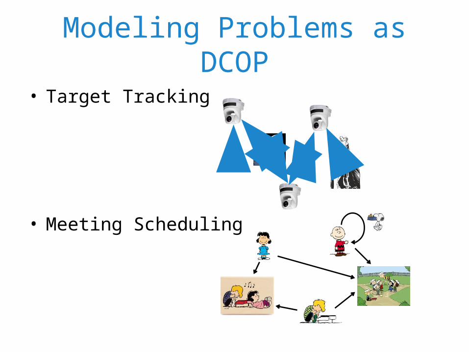
• Target Tracking

• Meeting Scheduling

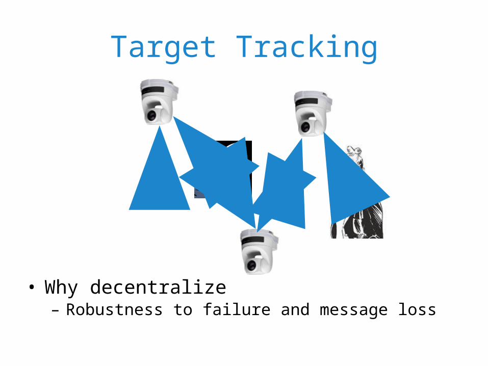
Target Tracking

• Why decentralize– Robustness to failure and message loss

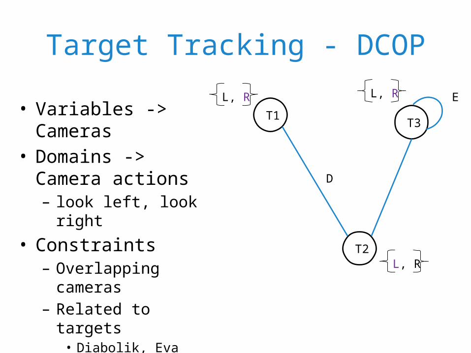
Target Tracking - DCOP

• Variables -> Cameras• Domains -> Camera

actions– look left, look right

• Constraints– Overlapping cameras– Related to targets

• Diabolik, Eva

• Maximise sum of constraints

L, R

L, R

L, R

D

E

T1

T2

T3

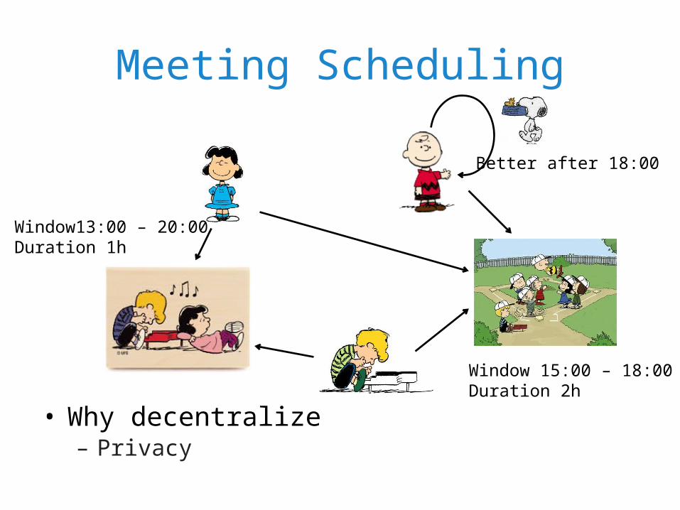
Meeting Scheduling

• Why decentralize– Privacy

Window 15:00 – 18:00Duration 2h

Window13:00 – 20:00Duration 1h

Better after 18:00

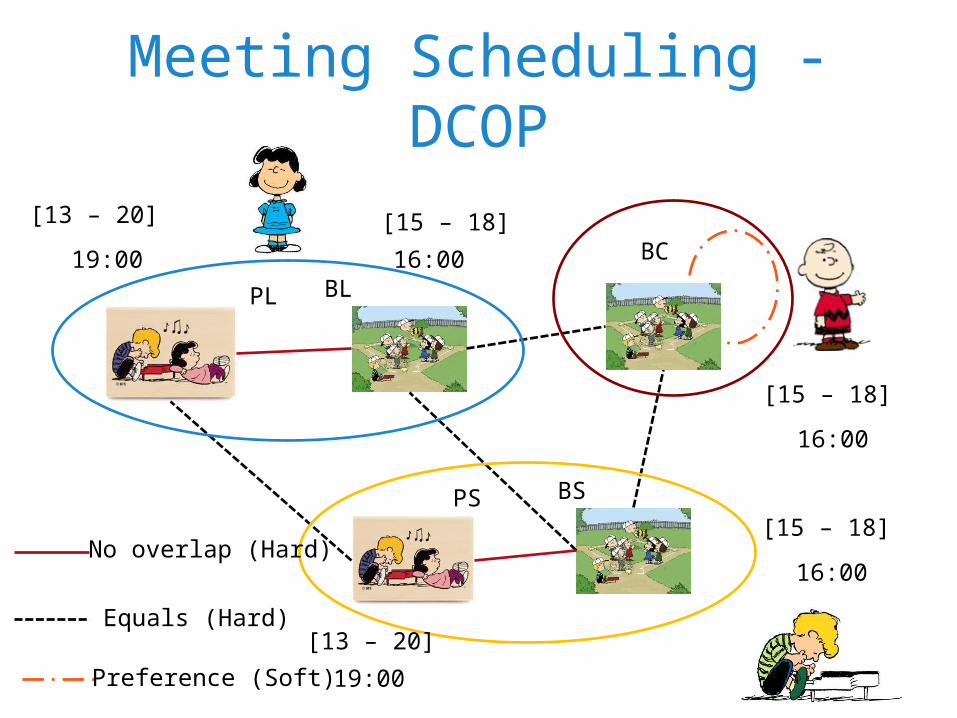
Meeting Scheduling - DCOP

PL

BSPS

BC

BL

No overlap (Hard)

Equals (Hard)

Preference (Soft)

16:00

16:0019:00

19:00

[15 – 18][13 – 20]

[13 – 20]

[15 – 18]

16:00

[15 – 18]

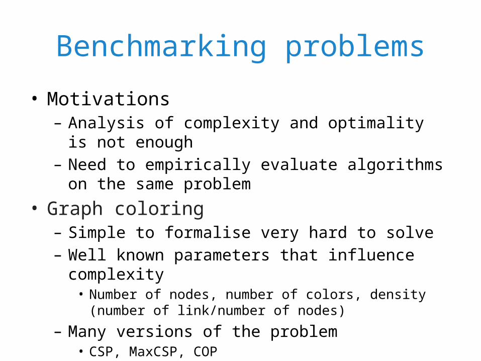
Benchmarking problems

• Motivations– Analysis of complexity and optimality is not enough– Need to empirically evaluate algorithms on the same

problem

• Graph coloring – Simple to formalise very hard to solve– Well known parameters that influence complexity

• Number of nodes, number of colors, density (number of link/number of nodes)

– Many versions of the problem• CSP, MaxCSP, COP

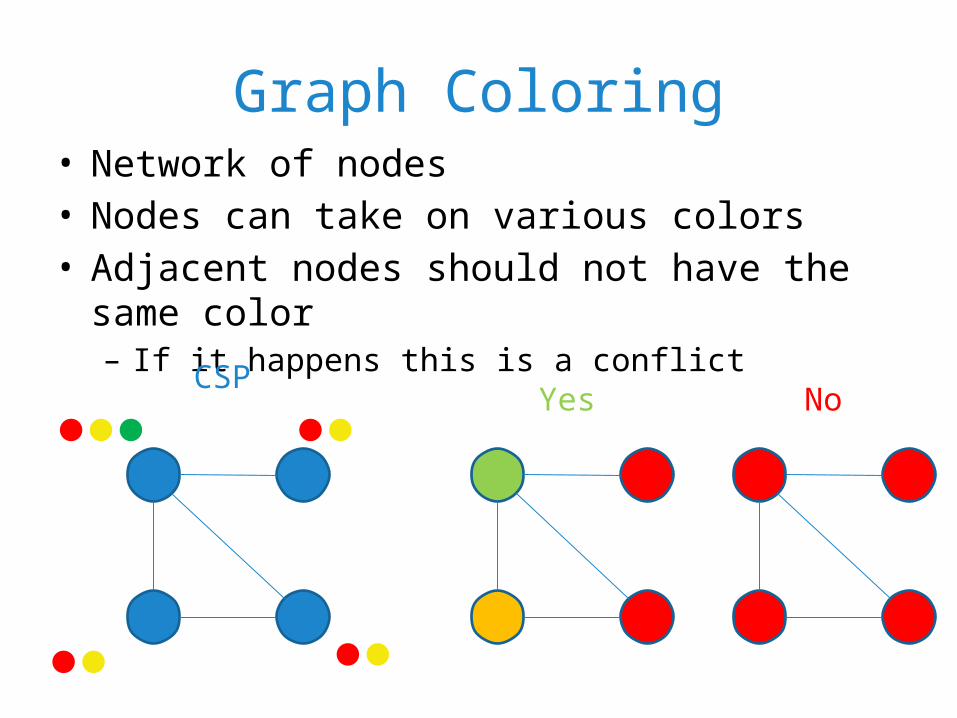
Graph Coloring• Network of nodes• Nodes can take on various colors• Adjacent nodes should not have the same color

– If it happens this is a conflict

CSPYes No

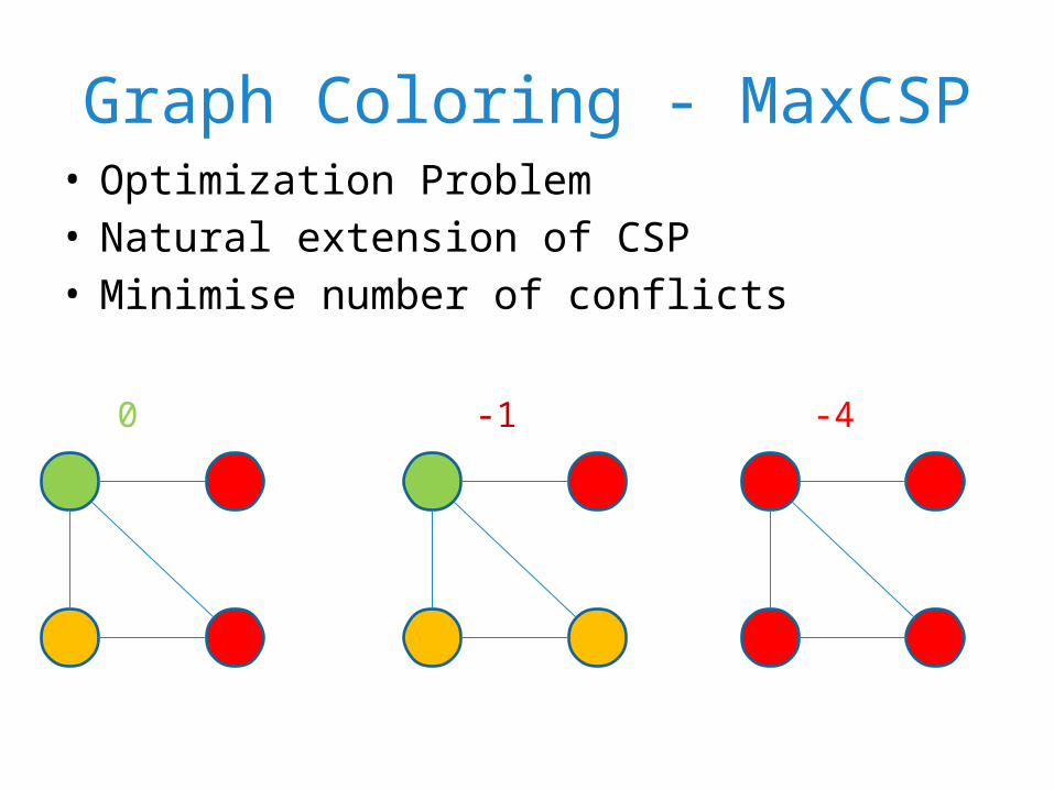
Graph Coloring - MaxCSP

0 -4

• Optimization Problem• Natural extension of CSP• Minimise number of conflicts

-1

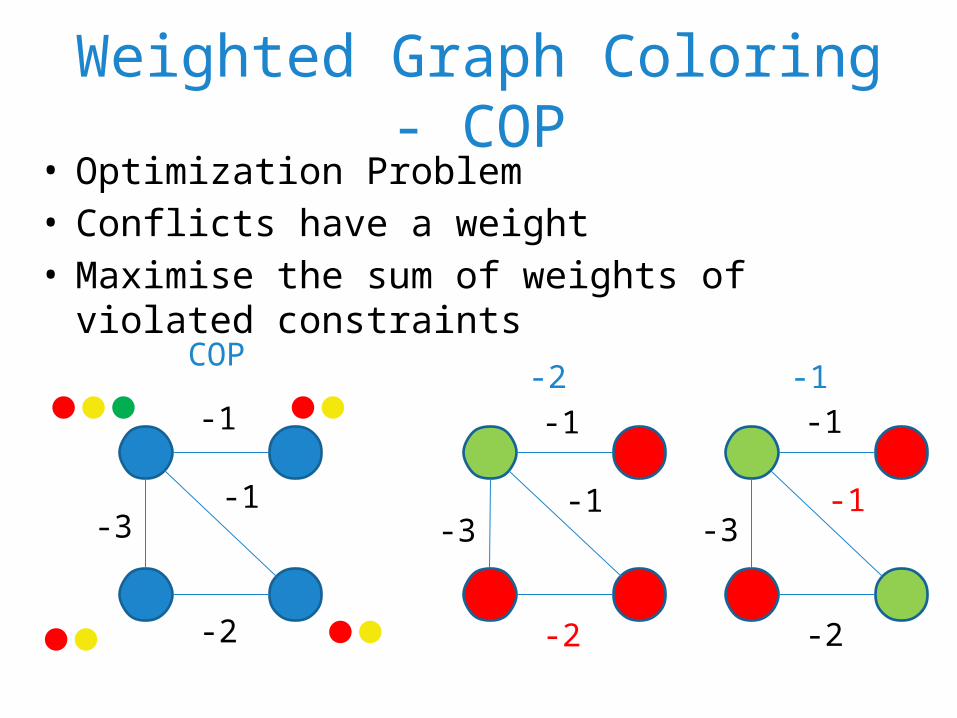
Weighted Graph Coloring - COP• Optimization Problem• Conflicts have a weight• Maximise the sum of weights of violated constraints

COP-2 -1

-1

-1

-2

-3

-1

-1

-2

-3

-1

-1

-2

-3

Distributed Constraint Optimization:Exact Algorithms

Pedro Meseguer

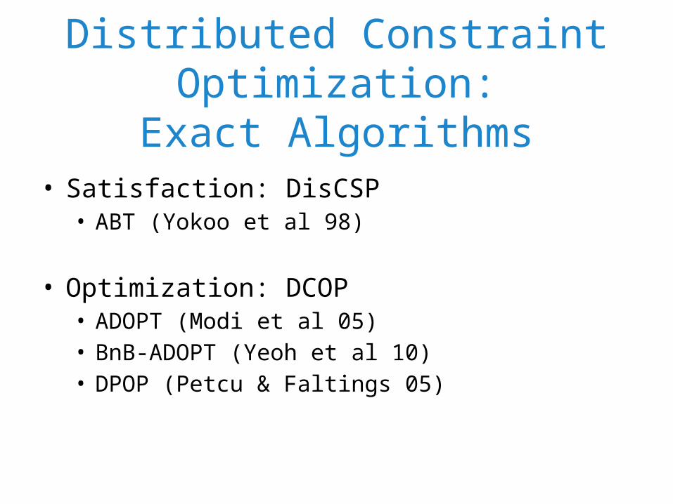
Distributed Constraint Optimization:Exact Algorithms

• Satisfaction: DisCSP• ABT (Yokoo et al 98)

• Optimization: DCOP• ADOPT (Modi et al 05)• BnB-ADOPT (Yeoh et al 10)• DPOP (Petcu & Faltings 05)

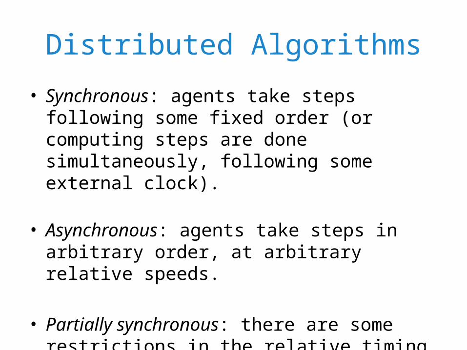
Distributed Algorithms

• Synchronous: agents take steps following some fixed order (or computing steps are done simultaneously, following some external clock).

• Asynchronous: agents take steps in arbitrary order, at arbitrary relative speeds.

• Partially synchronous: there are some restrictions in the relative timing of events

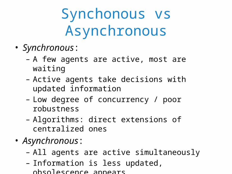
Synchonous vs Asynchronous

• Synchronous:– A few agents are active, most are waiting– Active agents take decisions with updated information– Low degree of concurrency / poor robustness– Algorithms: direct extensions of centralized ones

• Asynchronous:– All agents are active simultaneously– Information is less updated, obsolescence appears– High degree of concurrency / robust approaches– Algorithms: new approaches

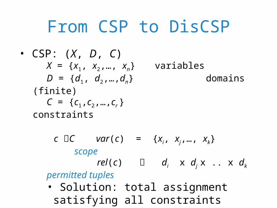
From CSP to DisCSP• CSP: (X, D, C)

X = {x1, x2,…, xn} variablesD = {d1, d2,…,dn} domains (finite)C = {c1,c2,…,cr } constraints

c C var(c) = {xi, xj,…, xk} scope rel(c) di x dj x .. x dk permitted tuples• Solution: total assignment satisfying all

constraints

• DisCSP: (X, D, C, A, ) A = {a1, a2,…, ak} agents : X -> A maps variables to agents

c is known by agents owning var(c)

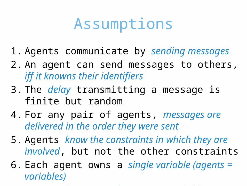
Assumptions

1. Agents communicate by sending messages2. An agent can send messages to others, iff it knowns

their identifiers3. The delay transmitting a message is finite but random4. For any pair of agents, messages are delivered in the

order they were sent5. Agents know the constraints in which they are involved,

but not the other constraints6. Each agent owns a single variable (agents = variables)7. Constraints are binary (2 variables involved)

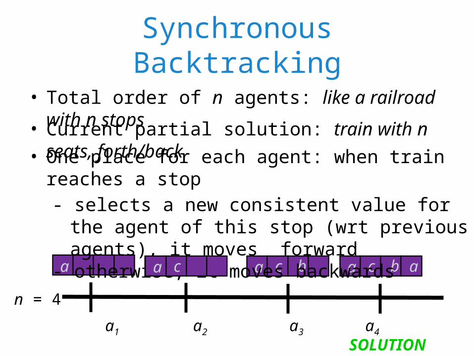
Synchronous Backtracking

• Total order of n agents: like a railroad with n stops

a1 a2 a3 a4

n = 4

a a a ca c b a c ba c b a

SOLUTION

• Current partial solution: train with n seats, forth/back• One place for each agent: when train reaches a stop

- selects a new consistent value for the agent of this stop (wrt previous agents), it moves forward

- otherwise, it moves backwards

a c

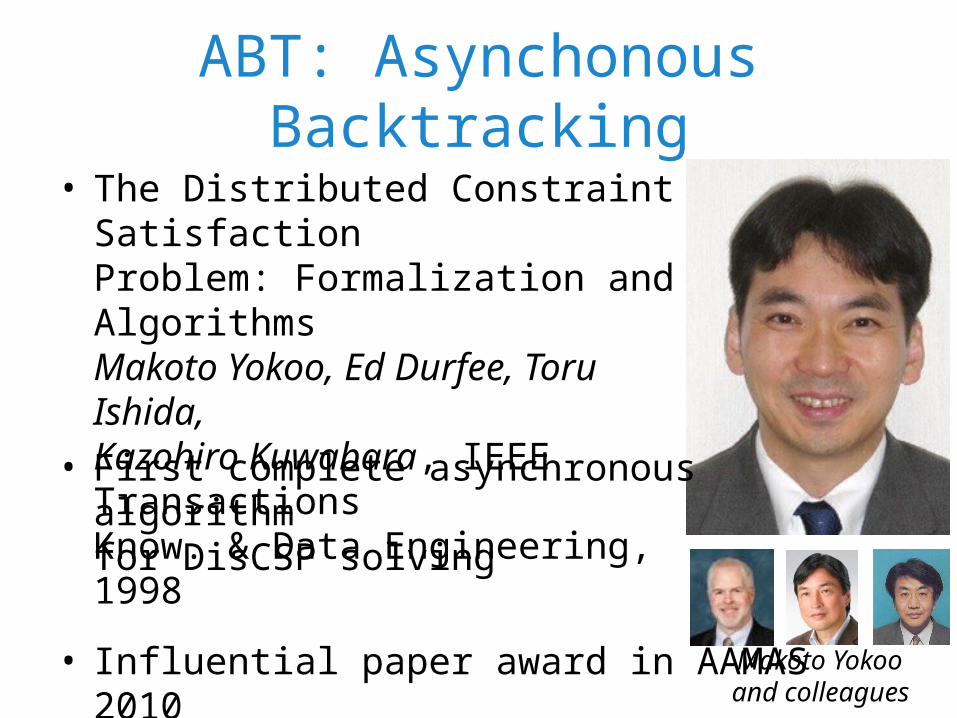
ABT: Asynchonous Backtracking• The Distributed Constraint Satisfaction

Problem: Formalization and AlgorithmsMakoto Yokoo, Ed Durfee, Toru Ishida,Kazohiro Kuwabara, IEEE Transactions Know. & Data Engineering, 1998

Makoto Yokoo and colleagues

• First complete asynchronous algorithm for DisCSP solving

• Influential paper award in AAMAS 2010

ABT: Description

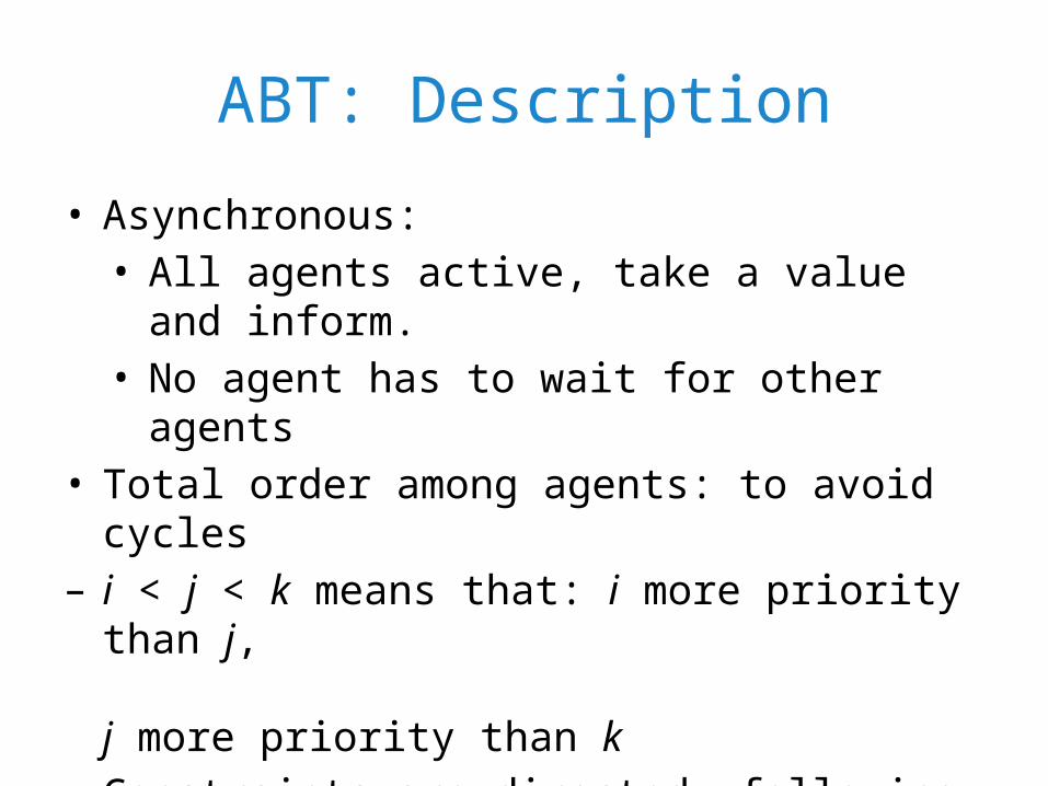
• Asynchronous:• All agents active, take a value and inform.• No agent has to wait for other agents

• Total order among agents: to avoid cycles– i < j < k means that: i more priority than j,

j more priority than k• Constraints are directed, following total order• ABT plays in asyncronous distributed context the

same role as backtracking in centralized

ABT: Directed Constraints

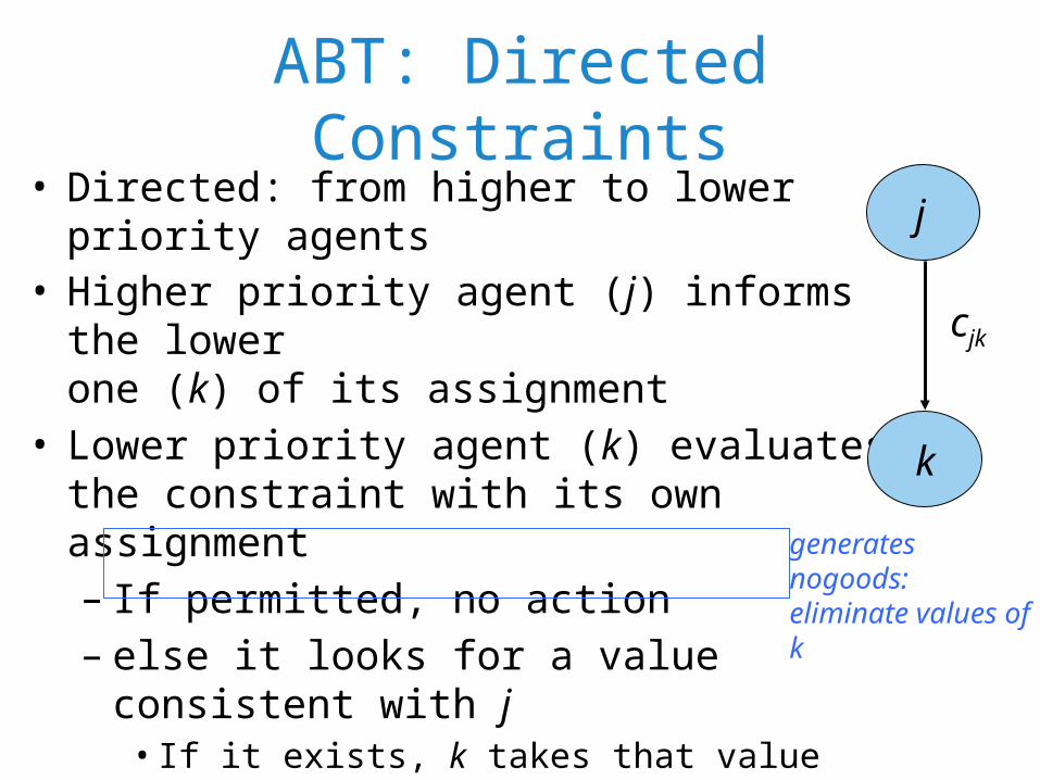
• Higher priority agent (j) informs the lowerone (k) of its assignment

• Lower priority agent (k) evaluates the constraint with its own assignment– If permitted, no action– else it looks for a value consistent with j

• If it exists, k takes that value• else, the agent view of k is a nogood, backtrack

generates nogoods:

eliminate values of k

j

k

cjk

• Directed: from higher to lower priority agents

ABT: Nogoods

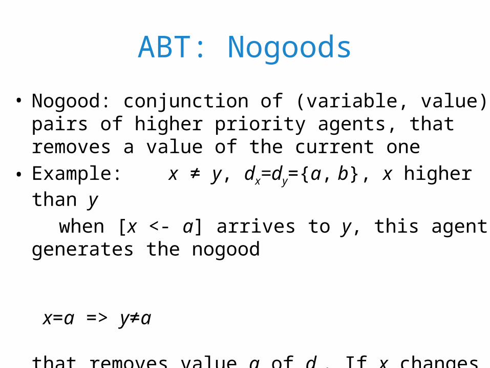
• Nogood: conjunction of (variable, value) pairs of higher priority agents, that removes a value of the current one

• Example: x ≠ y, dx=dy={a, b}, x higher than y

when [x <- a] arrives to y, this agent generates the nogood x=a => y≠a

that removes value a of dy. If x changes value, when [x <- b] arrives to y, the nogood x=a => y≠a is eliminated, value a is again available and a new nogood removing b is generated.

ABT: Nogood Resolution

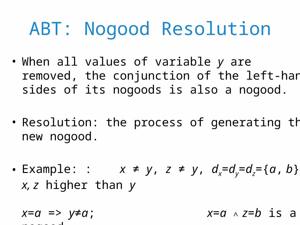
• When all values of variable y are removed, the conjunction of the left-hand sides of its nogoods is also a nogood.

• Resolution: the process of generating the new nogood.

• Example: : x ≠ y, z ≠ y, dx=dy=dz={a, b}, x, z higher than y

x=a => y≠a; x=a ∧ z=b is a nogood z=b => y≠b; x=a => z≠b (assuming x higher than z)

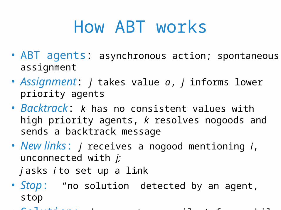
How ABT works• ABT agents: asynchronous action; spontaneous assignment

• Assignment: j takes value a, j informs lower priority agents

• Backtrack: k has no consistent values with high priority agents, k resolves nogoods and sends a backtrack message

• New links: j receives a nogood mentioning i, unconnected with j;j asks i to set up a link

• Stop: “no solution” detected by an agent, stop

• Solution: when agents are silent for a while (quiescence), every constraint is satisfied-> solution; detected by specialized algorithms

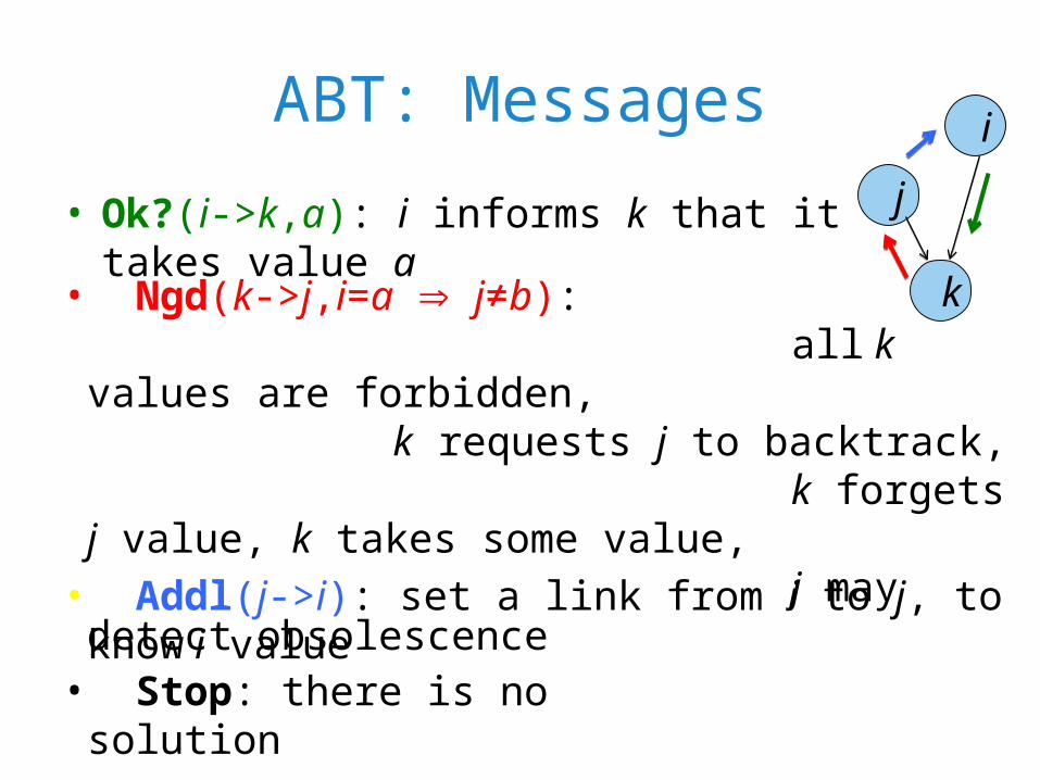
ABT: Messages

• Ok?(i->k,a): i informs k that it takes value a j

k

i

• Ngd(k->j,i=a j≠b): all k values are forbidden, k requests j to backtrack, k forgets j value, k takes some value, j may detect obsolescence

• Addl(j->i): set a link from i to j, to know i value

• Stop: there is no solution

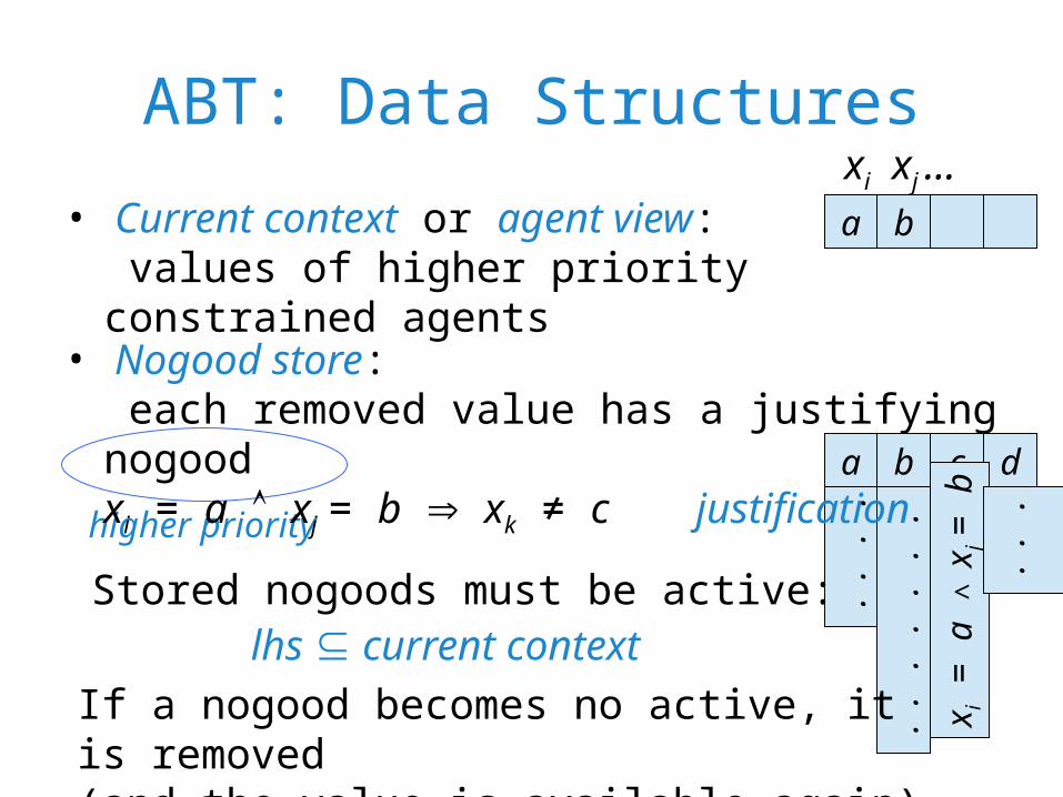
ABT: Data Structures

• Current context or agent view: values of higher priority constrained agents

higher priority

xi xj ...a b

a b c d

x i = a

∧ x j =

b

. .

.

. .

. .

.

. .

.

. .

.

• Nogood store: each removed value has a justifying nogoodxi = a xj = b xk ≠ c justification

Stored nogoods must be active: lhs current contextIf a nogood becomes no active, it is removed (and the value is available again)

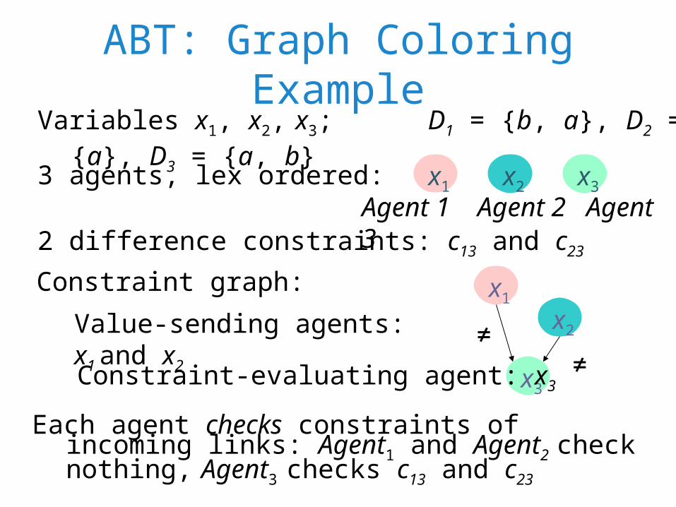
ABT: Graph Coloring Example

x1

Each agent checks constraints of incoming links: Agent1 and Agent2 check nothing, Agent3 checks c13 and c23

x2 x33 agents, lex ordered:

2 difference constraints: c13 and c23

Constraint graph: x1

x2

x3

≠≠

Variables x1, x2, x3; D1 = {b, a}, D2 = {a}, D3 = {a, b}

Agent 1 Agent 2 Agent 3

Value-sending agents: x1 and x2

Constraint-evaluating agent: x3

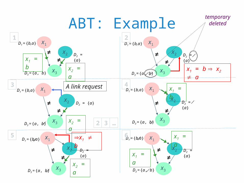
ABT: Example

x1 = b

x2 = a

x1

x2

x3

D1 = {b,a}

D2 = {a}

D3 = {a, b}

≠≠

1x1

x2

x3

D1 = {b,a}

D2 = {a}

D3 = {a, b}x1 = b x2 a

≠≠

2

x1

x2

x3

D1 = {b,a}

D2 = {a}

D3 = {a, b}

x1 = b

≠≠

4

D3 = {a, b}

x1

x2

x3

x1 b

x2 = a

D1 = {b,a}

D2 = {a}≠≠

5

x1 = a

x1

x2

x3

x1 = aD1 = {b,a}

D2 = {a}

D3 = {a, b}

≠≠

6

x2 = a

A link requestx1

x2

x3

D1 = {b,a}

D2 = {a}

D3 = {a, b}

≠≠

3

2 3 …

temporary deleted

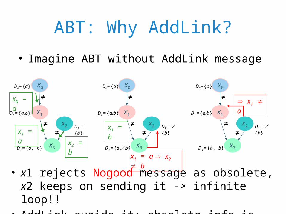
ABT: Why AddLink?

• Imagine ABT without AddLink message

x1 = a

x2 = b

x1

x2

x3

D1 = {a,b}

D2 = {b}

D3 = {a, b}

≠≠

x0D0= {a}

≠x0 = a

D1 = {a,b}

D3 = {a, b}

D0= {a}

x1

x2

x3

D2 = {b}≠≠

x0

≠

x1 = a x2 b

x1 = b

D1 = {a,b}

D3 = {a, b}

D0= {a}

x1

x2

x3

D2 = {b}≠≠

x0

≠ x1 a

• x1 rejects Nogood message as obsolete, x2 keeps on sending it -> infinite loop!!

• AddLink avoids it: obsolete info is removed in finite time

ABT: Correctness / Completeness

• Correctness: – silent network <=> all constraints are satisfied

• Completeness:– ABT performs an exhaustive traversal of the search space– Parts not searched: those eliminated by nogoods– Nogoods are legal: logical consequences of constraints– Therefore, either there is no solution => ABT generates the

empty nogood, or it finds a solution if exists

ABT: Termination

• There is no infinite loop• Induction in depth of the agent:

– Base case: the top agent x1 receives Nogood messages only, with empty left-hand side; either it discard all values, generating the empty nogood, or remains in a value; either case it cannot be in an infinite loop

– Induction case: assume x1 … xk-1 are in stable state, xk is loopingxk receives Nogood messages only containing x1 … xk

either it discards all values, generating a Nogood for x1 … xk-1

(breaking the assumption that x1 … xk-1 are in stable state) or it finds a consistent value (breaking the assumption that xk is in an infinite loop)

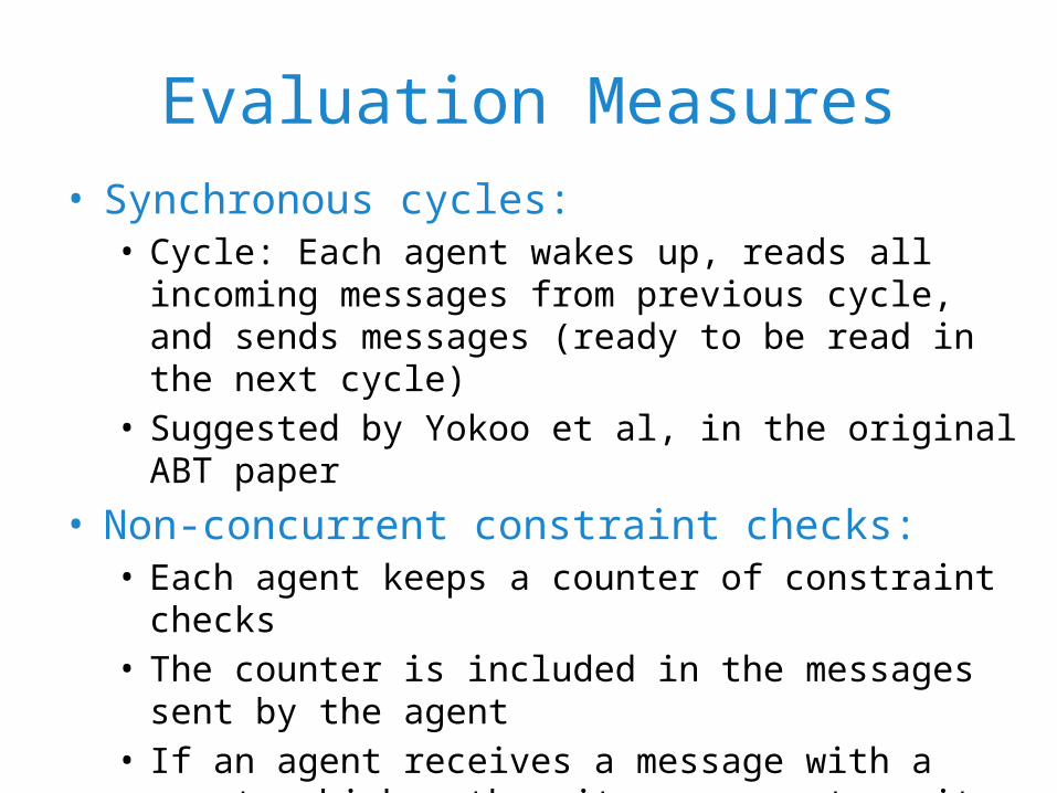
Evaluation Measures• Synchronous cycles:

• Cycle: Each agent wakes up, reads all incoming messages from previous cycle, and sends messages (ready to be read in the next cycle)

• Suggested by Yokoo et al, in the original ABT paper

• Non-concurrent constraint checks:• Each agent keeps a counter of constraint checks• The counter is included in the messages sent by the agent• If an agent receives a message with a counter higher than its

own counter, it copies the message counter• At the end, the highest counter is #NCCC • Suggested by Meisels et al, in 2002 (following logical clocks)

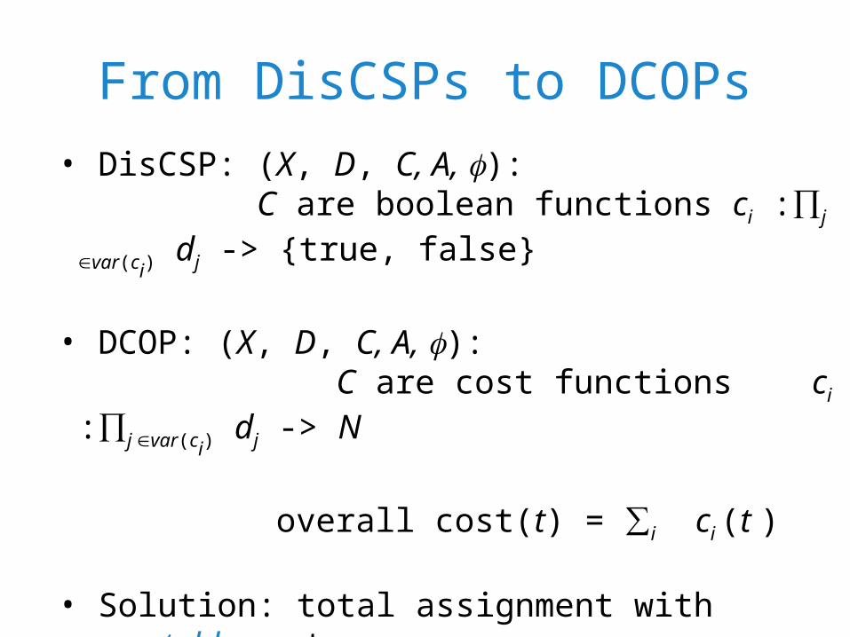
From DisCSPs to DCOPs• DisCSP: (X, D, C, A, ):

C are boolean functions ci :∏j var(ci) dj -> {true, false}

• DCOP: (X, D, C, A, ): C are cost functions ci :∏j var(ci)

dj -> N

overall cost(t) = ∑i ci (t )

• Solution: total assignment with acceptable cost

• Optimal solution: total assignment with minimum cost arg min ∑ij cij (t) (binary cost functions)

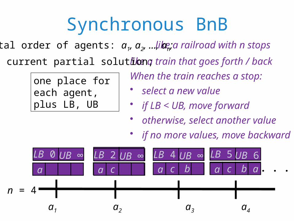
Synchronous BnB

a c bLB 0LB 4 UB ∞

a1 a2 a3 a4

n = 4

like a railroad with n stops

like a train that goes forth / back When the train reaches a stop:• select a new value• if LB < UB, move forward• otherwise, select another value• if no more values, move backward

LB 0 UB ∞a

LB 0 UB ∞a

LB 0 UB ∞a b

LB 0LB ∞ UB ∞a c

LB 0LB 2 UB ∞a c

LB 0LB 2 UB ∞a c b

LB 0LB 4 UB ∞a c b a

LB 0LB 5 UB 6 . . .

total order of agents: a1, a2, ..., an;

CPS: current partial solution;

one place for each agent,plus LB, UB

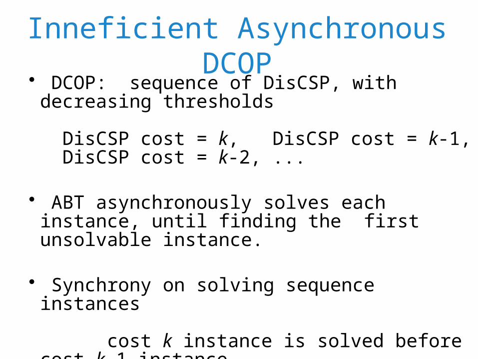
Inneficient Asynchronous DCOP• DCOP: sequence of DisCSP, with decreasing thresholds

DisCSP cost = k, DisCSP cost = k-1, DisCSP cost = k-2, ...

• ABT asynchronously solves each instance, until finding the first unsolvable instance.

• Synchrony on solving sequence instances

cost k instance is solved before cost k-1 instance

• Very inefficient

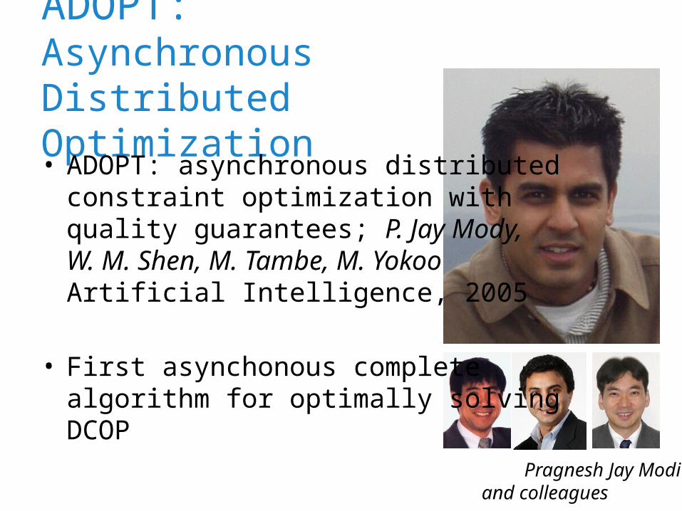
ADOPT: Asynchronous Distributed Optimization

Pragnesh Jay Modiand colleagues

• ADOPT: asynchronous distributed constraint optimization with quality guarantees; P. Jay Mody, W. M. Shen, M. Tambe, M. YokooArtificial Intelligence, 2005

• First asynchonous complete algorithm for optimally solving DCOP

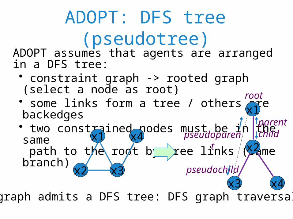
ADOPT: DFS tree (pseudotree)ADOPT assumes that agents are arranged in a DFS tree: • constraint graph -> rooted graph (select a node as root)• some links form a tree / others are backedges• two constrained nodes must be in the same path to the root by tree links (same branch)

Every graph admits a DFS tree: DFS graph traversal

x1

x2 x3

x4

x1

x2

x3 x4

parentchildpseudoparent

pseudochild

root

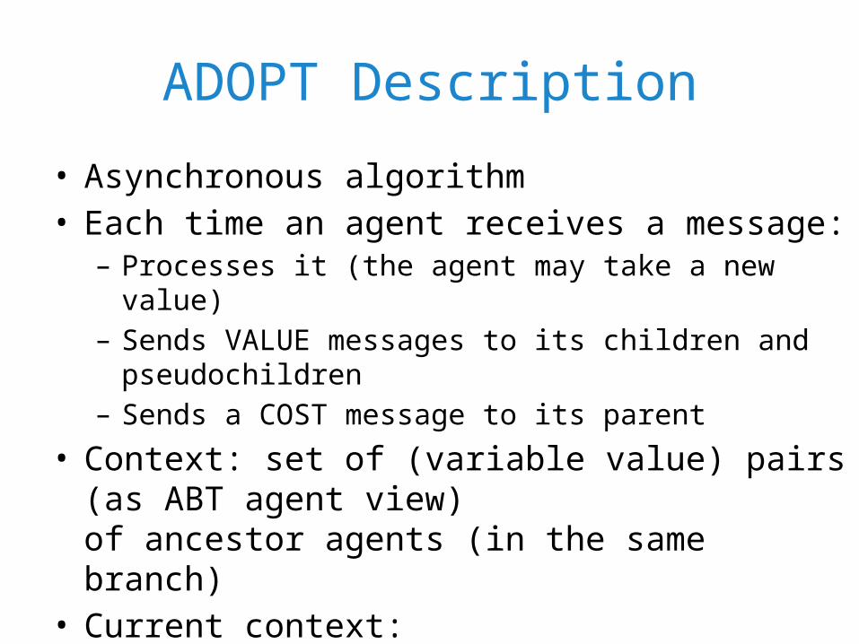
ADOPT Description

• Asynchronous algorithm• Each time an agent receives a message:

– Processes it (the agent may take a new value)– Sends VALUE messages to its children and pseudochildren– Sends a COST message to its parent

• Context: set of (variable value) pairs (as ABT agent view)of ancestor agents (in the same branch)

• Current context:– Updated by each VALUE message– If current context is not compatible with some child context,

the later is initialized (also the child bounds)

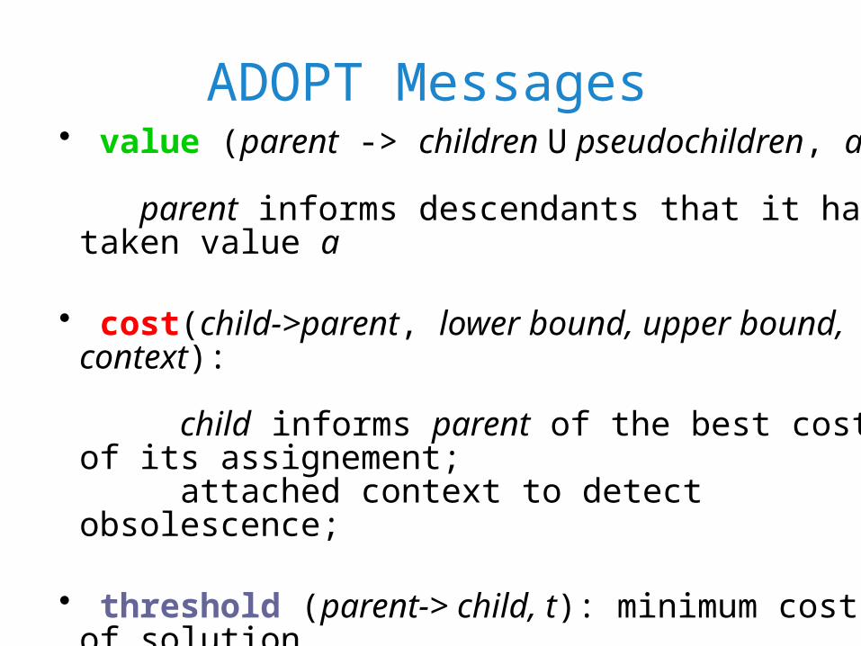
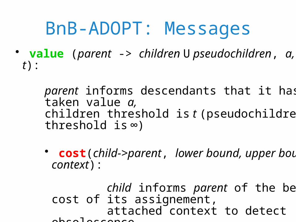
ADOPT Messages• value (parent -> children U pseudochildren, a):

parent informs descendants that it has taken value a

• cost(child->parent, lower bound, upper bound, context):

child informs parent of the best cost of its assignement; attached context to detect obsolescence;

• threshold (parent-> child, t): minimum cost of solution in child is at least t

• termination (parent-> children): LB = UB

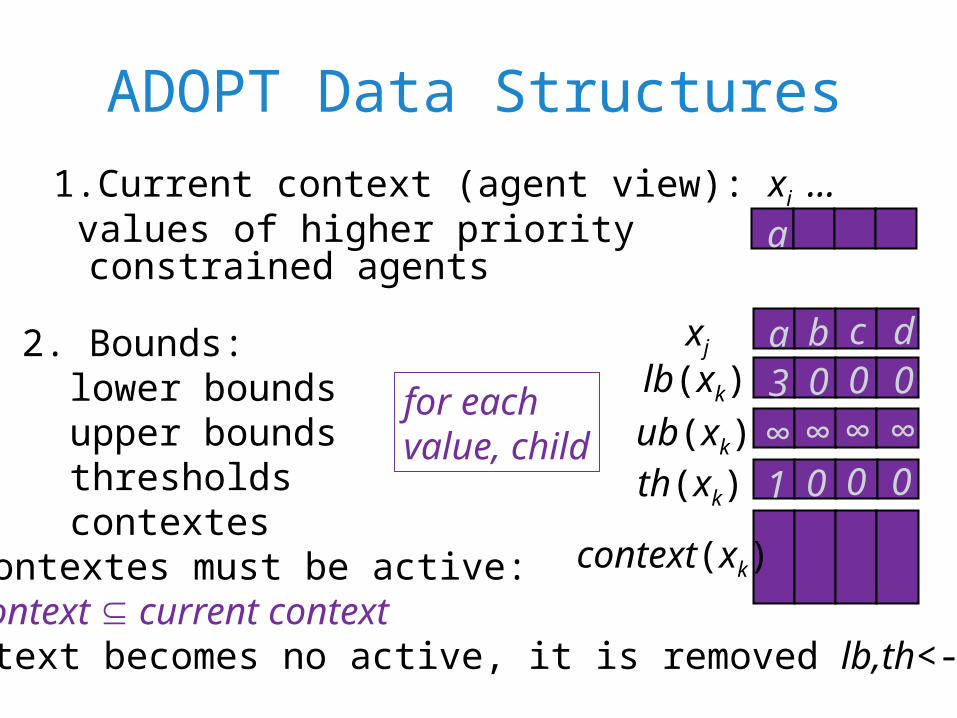
ADOPT Data Structures1.Current context (agent view):

values of higher priority constrained agents axi ...

2. Bounds:lower boundsupper boundsthresholdscontextes

Stored contextes must be active: context current contextIf a context becomes no active, it is removed lb,th<-0, ub<-∞

for each value, child

a b c d3 0 0 0∞ ∞ ∞ ∞

lb(xk)ub(xk)

xj

context(xk)

1 0 0 0th(xk)

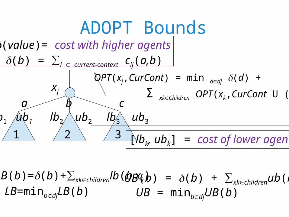
ADOPT Bounds

xj

21 3

a b clb1 ub1 lb2 ub2 lb3 ub3

[lbk, ubk] = cost of lower agents

LB(b)=(b)+∑xkchildrenlb(b,xk)LB=minbdjLB(b)

UB(b) = (b) + ∑xkchildrenub(b,xk)UB = minbdjUB(b)

OPT(xj,CurCont) = min ddj (d) +

Σ xkChildren OPT(xk,CurCont U (xj,d))

(b) = ∑i current-context cij(a,b)(value)= cost with higher agents

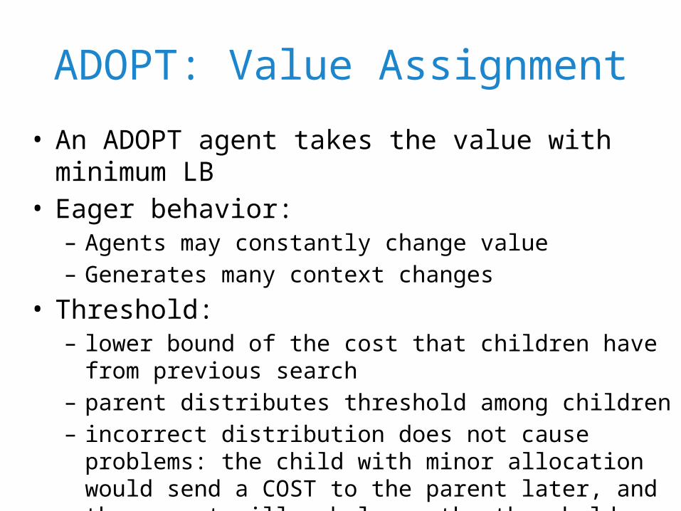
ADOPT: Value Assignment

• An ADOPT agent takes the value with minimum LB• Eager behavior:

– Agents may constantly change value– Generates many context changes

• Threshold: – lower bound of the cost that children have from previous search– parent distributes threshold among children– incorrect distribution does not cause problems: the child with

minor allocation would send a COST to the parent later, and the parent will rebalance the threshold distribution

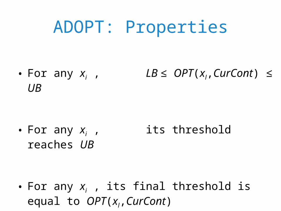
ADOPT: Properties

• For any xi , LB ≤ OPT(xl,CurCont) ≤ UB

• For any xi , its threshold reaches UB

• For any xi , its final threshold is equal to OPT(xl,CurCont)

[ADOPT terminates with the optimal solution]

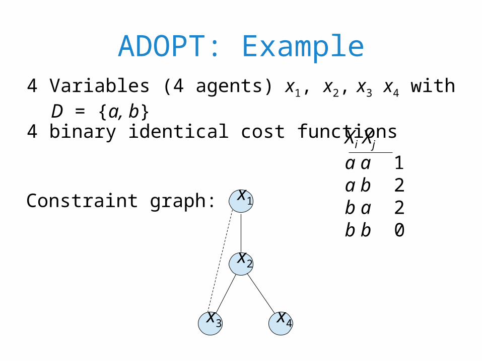
ADOPT: Example

4 binary identical cost functions

Constraint graph:

4 Variables (4 agents) x1, x2, x3 x4 with D = {a, b}

Xi Xj

a a 1a b 2b a 2b b 0

x1

x2

x3 x4

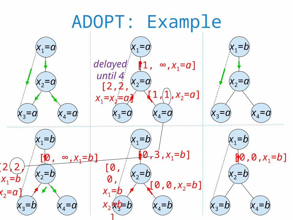
ADOPT: Examplex1=a

x2=a

x3=a x4=a

x1=b

x2=a

x3=a x4=a

x1=b

x2=b

x3=b x4=a

[0, ∞,x1=b][2,2,x1=bx2=a]

x1=b

x2=b

x3=b x4=b

[0,0,x1=bx2=b]

[0,0,x2=b]

[0,3,x1=b]

x1=b

x2=b

x3=b x4=b

[0,0,x1=b]

x1=a

x2=a

x3=a x4=a

[1,1,x2=a][2,2,

x1=x2=a]

[1, ∞,x1=a]delayeduntil 4

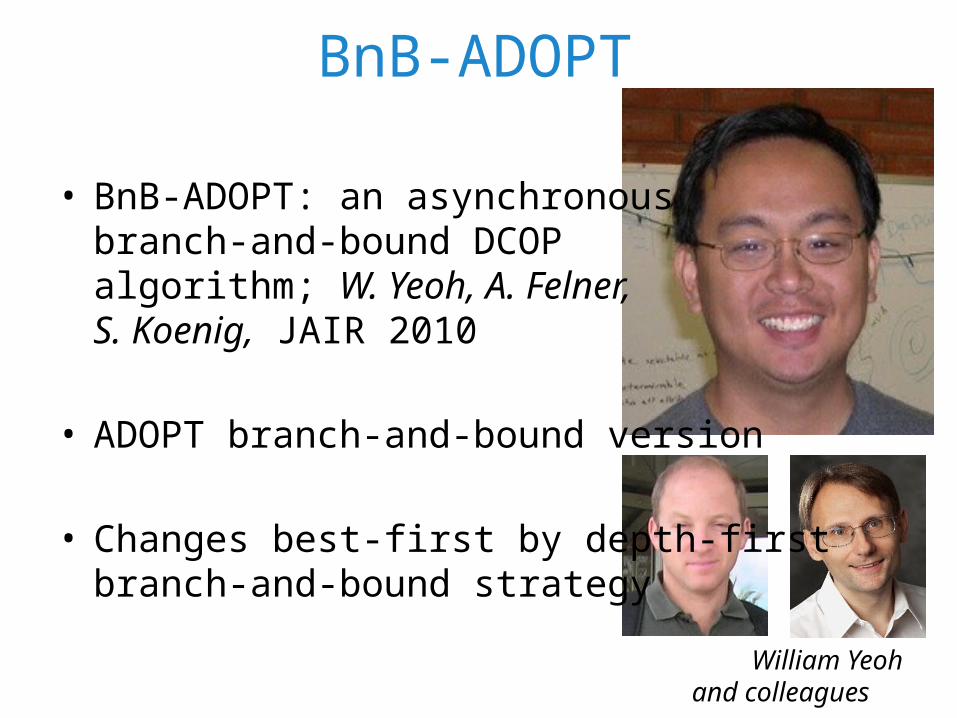
BnB-ADOPT

William Yeohand colleagues

• BnB-ADOPT: an asynchronous branch-and-bound DCOP algorithm; W. Yeoh, A. Felner, S. Koenig, JAIR 2010

• ADOPT branch-and-bound version

• Changes best-first by depth-first branch-and-bound strategy

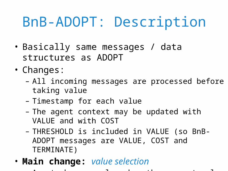
BnB-ADOPT: Description

• Basically same messages / data structures as ADOPT• Changes:

– All incoming messages are processed before taking value– Timestamp for each value – The agent context may be updated with VALUE and with COST– THRESHOLD is included in VALUE (so BnB-ADOPT messages are

VALUE, COST and TERMINATE)

• Main change: value selection– Agent changes value when the current value is definitely

worse than another value (LB(current-value) ≥ UB)– Thresholds are upper bounds (not lower bound like in ADOPT)

BnB-ADOPT: Messages• value (parent -> children U pseudochildren, a, t):

parent informs descendants that it has taken value a, children threshold is t (pseudochildren threshold is ∞)

• cost(child->parent, lower bound, upper bound, context):

child informs parent of the best cost of its assignement, attached context to detect obsolescence

• termination (parent-> children): LB = UB

x1=b

x2=b

x3=b x4=b

[0,0,x1=x2=b]

[0, ∞, x1=b]

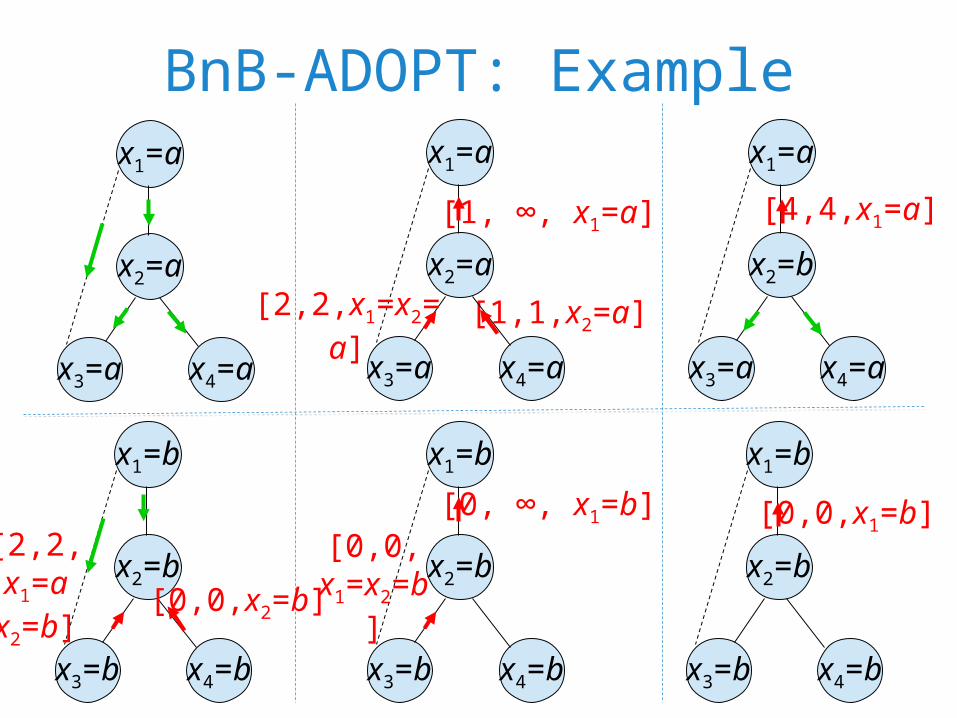
BnB-ADOPT: Examplex1=a

x2=a

x3=a x4=a

x1=b

x2=b

x3=b x4=b

[0,0,x1=b]

[1,1,x2=a]

x1=a

x2=a

x3=a x4=a

[2,2,x1=x2=a]

[1, ∞, x1=a]

x1=a

x2=b

x3=a x4=a

[4,4,x1=a]

x1=b

x2=b

x3=b x4=b

[2,2,x1=ax2=b]

[0,0,x2=b]

BnB-ADOPT: Performance

• BnB-ADOPT agents change value less frequently -> less context changes

• BnB-ADOPT uses less messages / less cycles than ADOPT

• Best-first strategy does not pay-off in terms of messages/cycles

BnB-ADOPT: Redundant Messages

• Many VALUE / COST messages are redundant

• Detection of redundant messages:[Gutierrez, Meseguer AAAI 2010]– VALUE to be sent: if it is equal to the last VALUE sent, it is

redundant– COST to be sent: if it is equal to the last COST sent and there is

no context change, it is redundant– For efficiency: take thresholds into account

• Significant decrement in #messages, keeping optimality

A New Strategy

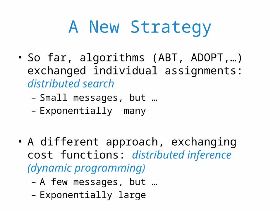
• So far, algorithms (ABT, ADOPT,…) exchanged individual assignments: distributed search– Small messages, but …– Exponentially many

• A different approach, exchanging cost functions: distributed inference (dynamic programming)– A few messages, but …– Exponentially large

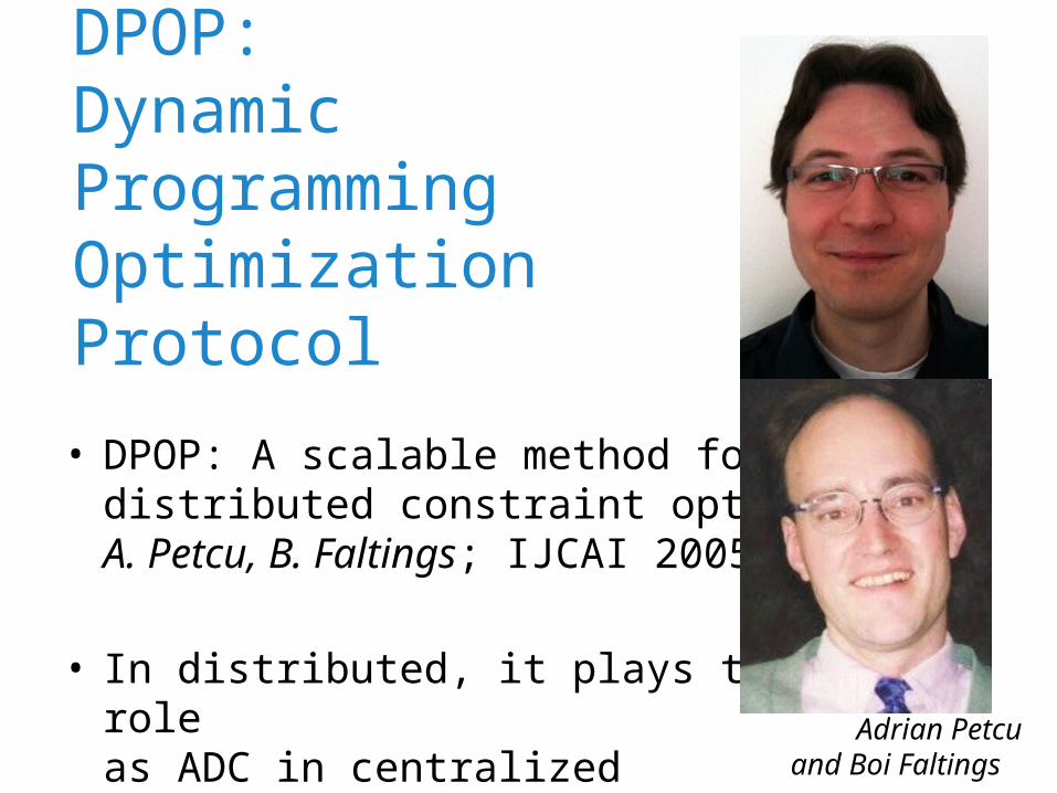
DPOP: Dynamic Programming Optimization Protocol

Adrian Petcuand Boi Faltings

• DPOP: A scalable method fordistributed constraint optimizationA. Petcu, B. Faltings; IJCAI 2005

• In distributed, it plays the same roleas ADC in centralized

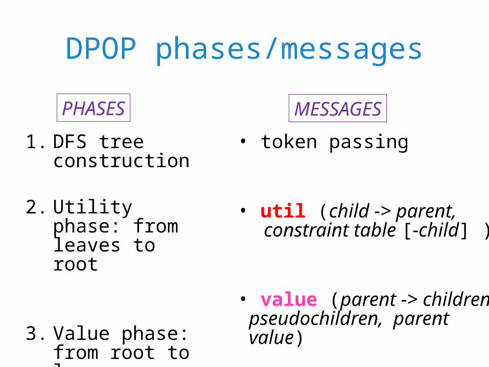
DPOP phases/messages

• token passing

• util (child -> parent, constraint table [-child] )

• value (parent -> children, pseudochildren, parent value)

1. DFS tree construction

2. Utility phase: from leaves to root

3. Value phase: from root to leaves

PHASES MESSAGES

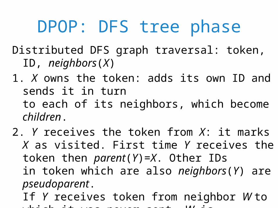
DPOP: DFS tree phaseDistributed DFS graph traversal: token, ID, neighbors(X)1. X owns the token: adds its own ID and sends it in turn

to each of its neighbors, which become children. 2. Y receives the token from X: it marks X as visited. First

time Y receives the token then parent(Y)=X. Other IDs in token which are also neighbors(Y) are pseudoparent. If Y receives token from neighbor W to which it was never sent, W is pseudochild.

3. When all neighbors(X) visited, X removes its ID from token and sends it to parent(X).

A node is selected as root, which starts. When all neighbors of root are visited, the DFS traversal ends.

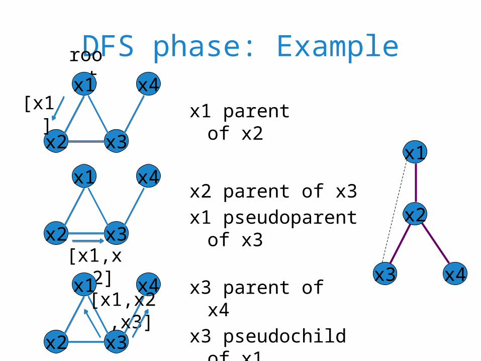
DFS phase: Exampleroot

x1

x2

x3 x4

x1

x2 x3

x4[x1] x1 parent of x2

x1

x2 x3

x4

[x1,x2]

x2 parent of x3x1 pseudoparent of x3

x1

x2 x3

x4[x1,x2,x3]

x3 parent of x4x3 pseudochild of x1

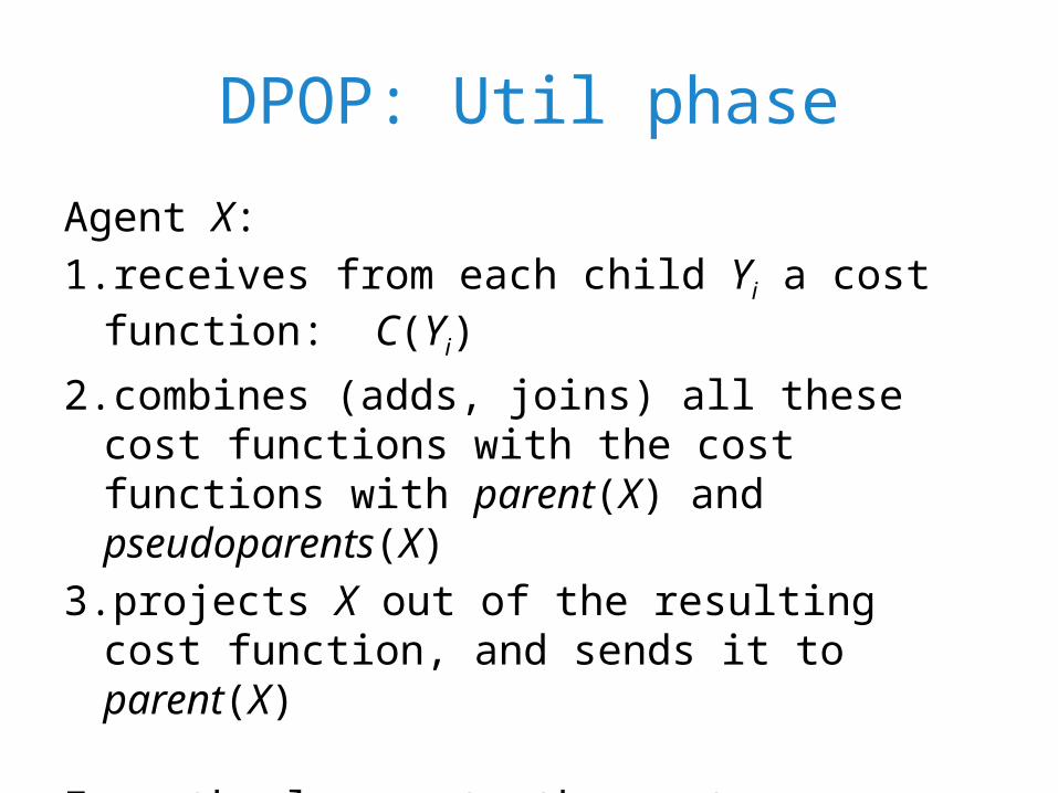
DPOP: Util phase

Agent X:1. receives from each child Yi a cost function: C(Yi)

2. combines (adds, joins) all these cost functions with the cost functions with parent(X) and pseudoparents(X)

3. projects X out of the resulting cost function, and sends it to parent(X)

From the leaves to the root.

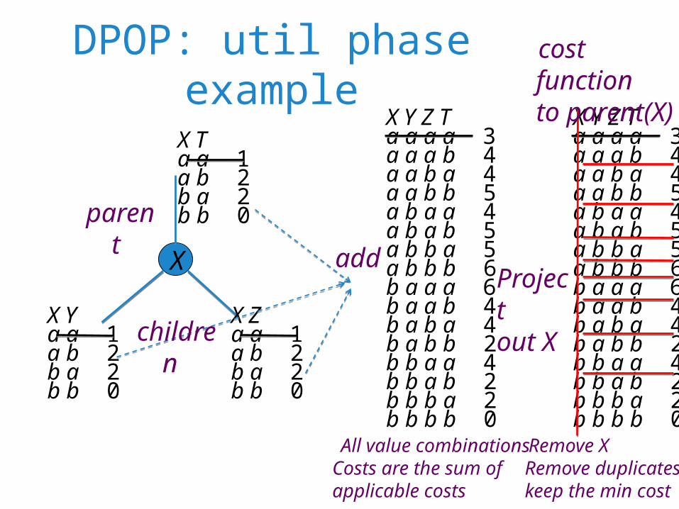
DPOP: util phase example

X

X Ya a 1a b 2b a 2b b 0

X Za a 1a b 2b a 2b b 0

X Ta a 1a b 2b a 2b b 0

X Y Z Ta a a a 3a a a b 4a a b a 4a a b b 5a b a a 4a b a b 5a b b a 5a b b b 6b a a a 6b a a b 4b a b a 4b a b b 2b b a a 4b b a b 2b b b a 2b b b b 0

parent

children

add Projectout X

X Y Z Ta a a a 3a a a b 4a a b a 4a a b b 5a b a a 4a b a b 5a b b a 5a b b b 6b a a a 6b a a b 4b a b a 4b a b b 2b b a a 4b b a b 2b b b a 2b b b b 0

All value combinations Costs are the sum of applicable costs

Remove XRemove duplicateskeep the min cost

cost function to parent(X)

DPOP: Value phase

1. The root finds the value that minimizes the received cost function in the util phase, and informs its descendants (children U pseudochildren)

2. Each agent waits to receive the value of its parent / pseudoparents

3. Keeping fixed the value of parent/pseudoparents, finds the value that minimizes the received cost function in the util phase

4. Informs of this value to its children/pseudochildren

This process starts at the root and ends at the leaves

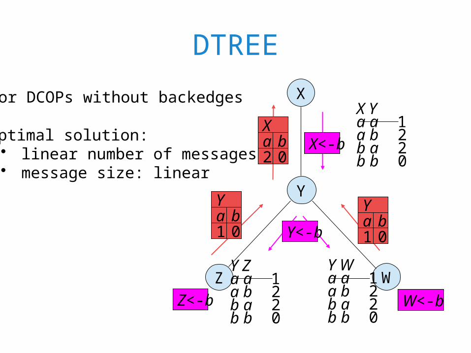
DTREE

X

Y

Z W

X Ya a 1a b 2b a 2b b 0

Y Wa a 1a b 2b a 2b b 0

Y Za a 1a b 2b a 2b b 0

1 0a bY

1 0a bY

2 0a bX

X<-b

Y<-b

For DCOPs without backedges

Z<-b W<-b

Optimal solution:• linear number of messages• message size: linear

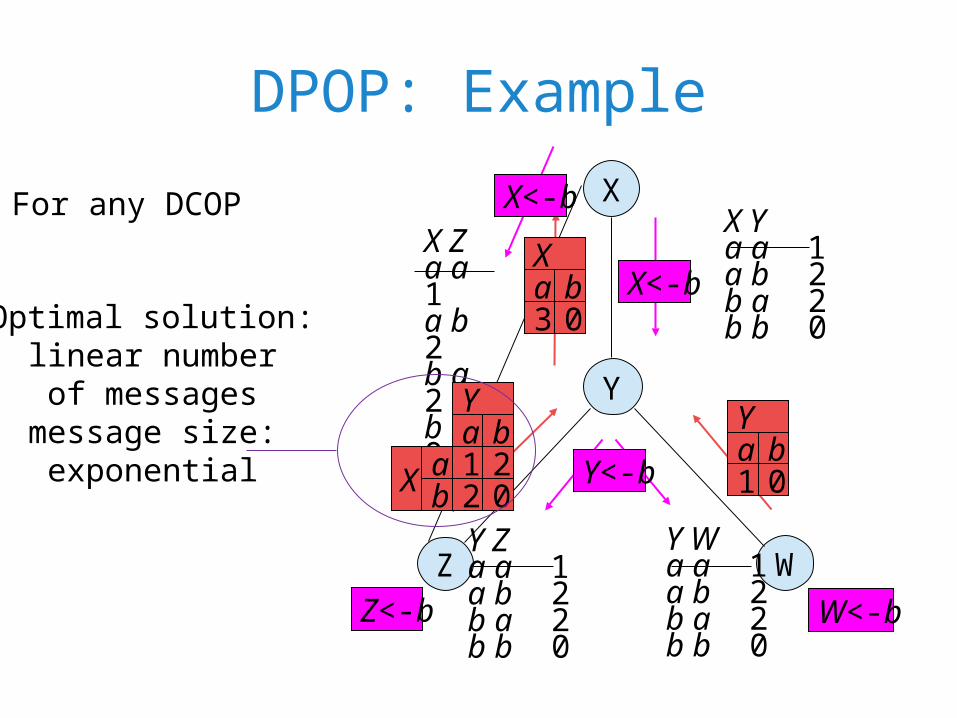
DPOP: Example

X

Y

Z W

1 0a bY

Y<-b

For any DCOP

Z<-b W<-b

Optimal solution:• linear number

of messages• message size:

exponential

X Ya a 1a b 2b a 2b b 0

Y Wa a 1a b 2b a 2b b 0

Y Za a 1a b 2b a 2b b 0

X Za a 1a b 2b a 2b b 0

1 2a bY

a2 0bX

3 0a bX

X<-b

X<-b

DPOP: Performance

• Synchronous algorithm, linear number of messages

• util messages can be exponentially large: main drawback

• Function filtering can alleviate this problem

• DPOP completeness: direct, from Adaptive Consistency results in centralized