A particle swarm optimization approach for constraint ...niadr/PUBLICATIONS/LIACC_publications... · ORIGINAL ARTICLE A particle swarm optimization approach for constraint joint single

ORIGINAL ARTICLE

A particle swarm optimization approach for constraint jointsingle buyer-single vendor inventory problem with changeablelead time and (r,Q) policy in supply chain

Ata Allah Taleizadeh & Seyed Taghi Akhavan Niaki &Nima Shafii & Ramak Ghavamizadeh Meibodi &Armin Jabbarzadeh

# Springer-Verlag London Limited 2010

Abstract In this paper, the chance-constraint joint singlevendor-single buyer inventory problem is considered in whichthe demand is stochastic and the lead time is assumed to varylinearly with respect to the lot size. The shortage incombination of back order and lost sale is considered and thedemand follows a uniform distribution. The order should beplaced in multiple of packets, the service rate limitation oneach product is considered a chance constraint, and there is alimited budget for the buyer to purchase the products. The goalis to determine the re-order point and the order quantity of eachproduct such that the chain total cost is minimized. The model

of this problem is shown to be an integer nonlinearprogramming type and in order to solve it, a particle swarmoptimization (PSO) approach is used. To assess the efficiencyof the proposed algorithm, the model is solved using bothgenetic algorithm and simulated annealing approaches as well.The results of the comparisons by a numerical example, inwhich a sensitivity analysis on the model parameters is alsoperformed, show that the proposed PSO algorithm performsbetter than the other two methods in terms of the total supplychain costs.

Keywords Multi-product inventory . Stochastic demand .

Changeable lead time . Supply chain . Integer nonlinearprogramming . Particle swarm optimization

1 Introduction and literature review

As the firms realize that a more efficient management ofinventories across the entire supply chain through bettercoordination and more cooperation are in the jointbenefit of all parties involved, the joint single-vendorsingle-buyer inventory problem (J-SVSB-IP) has receivedan extensive attention in the literature. While some of theprevious research on the joint vendor-buyer problemfocused on the production shipment with constant demandand lead time, in some research there is no constraint andthe simplest form of the joint single vendor-single buyerproblem is assumed.

One of the earliest researches on the J-SVSB-IP is due toBanerjee [3], in which he assumed that the vendor played therole of a manufacturing company with a finite production rateand considered a lot-for-lot model to satisfy the buyerrequests as separate batches. Moreover, various types of J-

A. A. Taleizadeh :A. JabbarzadehDepartment of Industrial Management,Raja University,Qazvin, Iran

A. A. Taleizadehe-mail: [email protected]

A. Jabbarzadehe-mail: [email protected]

S. T. A. Niaki (*)Department of Industrial Engineering,Sharif University of Technology,P.O. Box 11155-9414, Azadi Ave.,Tehran 1458889694, Irane-mail: [email protected]

N. ShafiiFaculty of Engineering, University of Porto,Rua Dr. Roberto Frais,Porto, Portugale-mail: [email protected]

R. G. MeibodiDepartment of Electrical and Computer Engineering,Shahid Beheshti University,Tehran, Irane-mail: [email protected]

DOI 10.1007/s00170-010-2689-0Int J Adv Manuf Technol (2010) 51:1209–1223

Received: 13 December 2008 /Accepted: 20 April 2010 /Published online: 15 May 2010

SVSB-IP were considered by Goyal [12], Goyal and Gupta[13], and Lu [30]. Hill [18] investigated an unequal shipmentpolicy for the J-SVSB-IP and concluded that an optimalpolicy for this problem is to use shipment sizes that increaseby a fixed factor in the beginning and then remainingconstant after a well-specified number of shipments. Ouyanget al. [32] extended the Ben-Daya and Raouf’s [4] model inwhich shortages were allowed and the total amount of stock-outs was considered as a mixture of back orders and lostsales. Hsiao and Lin [19] investigated an economic orderquantity model on Stackelberg game in supply chain; that is,a distribution channel system containing one supplier and asingle retailer such that the supplier in the channel holdsmonopolistic status, in which he not only owns costinformation about the retailer but also has the decisionmaking right of the lead time. Hariga and Ben-Daya [16]developed a continuous review inventory model where thereorder point, the ordering quantity, and the lead time werethe decision variables.

On the joint single-vendor multiple-buyer inventoryproblem, Siajadi et al. [38] presented a new methodology toobtain the joint economic lot size in the case where multiplebuyers are demanding one type of item from a single vendor.They found the shipment policy and proposed a new modelto minimize the joint total relevant cost for both vendor andbuyer(s). Wee and Yang [48] developed an optimal pricingand replenishment policies in a supply chain system for asingle vendor and multiple buyers. They showed since itbenefits the vendor more than the buyers in the integratedsystem, a pricing strategy with price reduction is incorporat-ed to entice the buyers to accept the minimum total costintegrated system. Kim et al. [24] proposed centralized anddecentralized adaptive inventory control models for a supplychain consisting of one supplier and multiple retailers. Theobjectives of the models were to satisfy a target service levelpredefined for each retailer. The inventory-control parame-ters of the supplier and retailers were safety lead time andsafety stocks, respectively.

For more complex supply chains, Su et al. [39] considereda chain system where facilities produce intermediate or enditems that were shipped to other facilities or customers. Theyconsidered a complicated production process that can beconvergent, divergent, and circulatory. Moreover, Heydari etal. [17] investigated lead time variability in a seriallyconnected supply chain with four levels.

On the variable lead time researches, Lodree et al. [29]investigated a supply chain system in an uncertain demandand variable lead time setting that encompasses customerwaiting costs as well as traditional plant costs (i.e.,production and inventory costs). Wang [47] provided a studyof examining two aspects of supply chain flexibility: orderquantity and lead time flexibilities, which have been clarified

as the two most common changes which occur in supplychains. Wu [49] analytically studied the implication of acontrollable lead time and a random supplier capacity on thecontinuous review inventory policy, in which the orderquantity, reorder point, and lead time were decisionvariables. Ouyang and Chuang [33] considered a mixtureperiodic review inventory model in which both the lead timeand the review period were considered decision variables.Instead of having a stock-out term in the objective function,a service level constraint was added to the model.

Meta-heuristic algorithms have been proposed to solvesome of the existing developed inventory models in theliterature. Some of these algorithms are: simulating annealing[1, 40], threshold accepting [7], Tabu search [20], geneticalgorithms [2, 41, 44], neural networks [9], ant colonyoptimization [6], fuzzy simulation [43], evolutionary algo-rithm [25, 45], and harmony search [10, 26, 42]. Examplesof researches on particle swarm optimization (PSO) algo-rithm can be found in [14, 27, 36, 50], and Rahimi-Vahed etal. [34]. Furthermore, there are some applications of the PSOalgorithm on constraint programming of supply chainproblems in the literature (see for example [21, 51]).

In this paper, a constraint joint single vendor-singlebuyer inventory problem is considered in which besides theassumptions of Ben-Daya and Hariga [5] research, thedemand follows a uniform probability distribution, the leadtime is variable, and there exists a linear relation betweenthe lead time and the lot size. Furthermore, the improve-ments of the current research over the Ben-Daya andHariga’s research [5] are: (1) a combination of back orderand lost sale is considered, (2) service rate is a chance-constraint for each product, (3) multi-product inventorysystem is assumed, (4) orders should be placed in multipleof packets, (5) the buyer has a limited budget to purchasethe products, and (6) a different meta-heuristic solutionalgorithm is proposed to solve the model.

The remainder of the paper is organized as follows. InSection 2, the problem is defined in details. While inSection 3, the problem is modeled, the meta-heuristicsolution algorithm of particle swarm is presented insection 4. Section 5 contains a numerical example alongwith the obtained benchmarking the model using differentmeta-heuristic algorithms. In Section 6, the proposed PSOalgorithm is illustrated for the given numerical example.Section 7 contains a sensitivity analysis on the modelparameters, and finally the conclusion comes in Section 8.

2 Problem definition

Consider a J-SVSB-IP in which the buyer is using theclassical (r, Q) continuous review inventory policy and

1210 Int J Adv Manuf Technol (2010) 51:1209–1223

the demand is stochastic. Assume that the lead time is afunction of the production lot size. In particular, let thelead time of each product be proportional to thecorresponding lot size produced by the vendor plus afixed delay due to transportation, nonproductive time,etc.

The relationship between the vendor and the buyer isdescribed as follows: for the ith product, i=1, 2,..., p, thebuyer orders a lot of size Qi to the vendor and incurs anordering cost Ai. The vendor manufactures the product inlots with a finite production rate Pi and incurs a setup costCAv . Then, the buyer receives noi shipments, each contain-ing Mi packets of ni products, Qi=niMi, and incurs atransportation cost for each shipment At

i. The buyer placeshis order when his on-hand inventory of the ith productreaches a reorder point ri. Moreover, there are lower limitson the service rate of each product as chance constraintsand that the buyer has a limited amount of budget topurchase the products TB. Shortages are allowed and incurin combination of back order and lost sale. The elementsof the buyer cost function are fixed order, holding,shortage, and transportation costs. The transportation costis constant for each shipment. For the vendor, the set-upand holding costs are considered. The objective of thisresearch is to determine the reorder points, the orderquantities and the number of shipments for each productsuch that the expected total cost of the supply chain isminimized.

3 Modeling

To model the problem, let us to first define the parameters andthe variables of the model. Then based on these definitions,the buyer's, the vendor's, and the chain total costs are derivedin Sections 3.2, 3.3, and 3.4, respectively. The constraints arenext introduced in Section 3.5, and finally the mathematicalmodel of the problem is given in Section 3.6.

3.1 Parameters and variables

For a specific product i, i=1, 2,..., p, let define theparameters and the variables of the model as:

ri reorder point of the ith product (a decision variable)noi number of shipments of the ith product from the

vendor to the buyer (a decision variable)Mi expected number of the packets for the ith

product order (a decision variable)ni number of the ith product in each packetQi expected amount of the ith product order (a

decision variable in which, Qi=niMi)

SSi safety stock of the ith product (a decision variable)Di expected demand quantity of the ith product, i.e.,

Di ¼ DMini þDMax

i2

fDi dið Þ probability density functions of Di (a Uniformdensity function with parameters DMin

i , DMaxi )

Pi constant production rate of the ith product (Pi≥Di)SLi the lower limit of the service level for the ith

productβi percentage of unsatisfied demands of the ith

product that is back orderedπi the back-order cost per unit demand of the ith productbpi shortage cost for each unit of the ith product that

is lost saleAi constant cost per order of the ith productAti buyer's constant transportation cost per shipment

of the ith productApi buyer's constant production cost for each setup of

the ith producthvi vendor's holding cost per unit time per unit of the

ith producthbi buyer's holding cost per unit time per unit of the

ith productbi r;Qð Þ expected amount of the ith product shortageBi expected amount of the ith product back order

Bi ¼ bibi r;Qð Þ� �Li Expected amount of the ith product lost sale

Li ¼ 1� bið Þbi r;Qð Þ� �Ii expected amount of the ith product inventoryLTi the ith product lead time is assumed to be

LTi ¼ Qi

Piþ gi, where γi denotes a fixed delay due

to transportation, production time of otherproducts scheduled during the lead time on thesame facility, etc.

TB buyer's total available budgetCi purchasing price per unit of the ith productCHb expected total holding cost of the buyerCHv total holding cost of the vendorCBb buyer's expected total shortage cost in back-order

stateCLb buyer's expected total shortage cost in lost sale stateCAb buyer's expected total order costCAv vendor's expected total set up costCTb buyer's expected total transportation costTCb buyer's expected total costTCv vendor's expected total costTC expected total cost of the supply chain

3.2 The buyer's total costs

In spite of Ben-Daya and Hariga [5] who modeled the J-SVSB-IP in the case of the stochastic demand and variable

Int J Adv Manuf Technol (2010) 51:1209–1223 1211

lead time, in this research, the J-SVSB-IP is formulated:allowing shortages as combinations of back orders and lostsales. Furthermore, there exit transportation costs; servicerate is a chance-constraint for each product; multi-productinventory system is assumed; orders should be placed inmultiple of packets, and the buyer has a limited budget topurchase the products. To model the problem, a model for asingle product i is first developed and then it is extended toinclude several products.

The buyer's total expected cost per unit time is given by:

TCb ¼ CAb þ CHb þ CBb þ CLb þ CTb ð1Þ

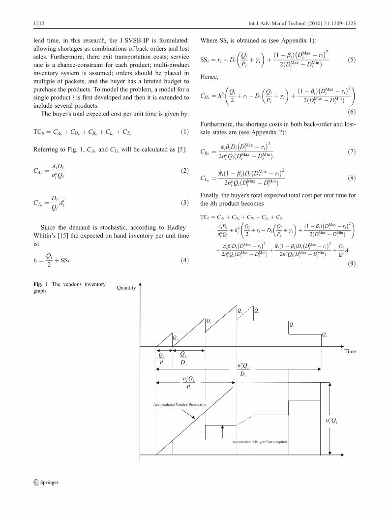
Referring to Fig. 1, CAb and CTb will be calculated as [5]:

CAb ¼AiDi

noi Qið2Þ

CTb ¼Di

QiAti ð3Þ

Since the demand is stochastic, according to Hadley–Whitin’s [15] the expected on hand inventory per unit timeis:

Ii ¼ Qi

2þ SSi ð4Þ

Where SSi is obtained as (see Appendix 1):

SSi ¼ ri � DiQi

Piþ gi

� �þ 1� bið Þ DMax

i � ri� �2

2 DMaxi � DMin

ið Þ ð5Þ

Hence,

CHb ¼ hbiQi

2þ ri � Di

Qi

Piþ gi


i � ri� �2

2 DMaxi � DMin

ið Þ

!ð6Þ

Furthermore, the shortage costs in both back-order and lost-sale states are (see Appendix 2):

CBb ¼pibiDi DMax

i � ri� �2

2noi Qi DMaxi � DMin

ið Þ ð7Þ

CLb ¼bpi 1� bið ÞDi DMax

i � ri� �2


ið Þ ð8Þ

Finally, the buyer's total expected total cost per unit time forthe ith product becomes

TCb ¼ CAb þ CHb þ CBb þ CLb þ CTb

¼ AiDi

noi Qiþ hbi

Qi

2þ ri � Di

Qi

Piþ gi


i � ri� �2

2 DMaxi � DMin

ið Þ

!

þ pibiDi DMaxi � ri

� �22noi Qi DMax

i � DMinið Þ þ

bpi 1� bið ÞDi DMaxi � ri


i � DMinið Þ þ Di

QiAti

ð9Þ

Accumulated Buyer Consumption

Accumulated Vendor Production

oi in Q

oi i

i

n Q

P

i

i

Q

P i

i

Q

D

oi i

i

n Q

D

iQ

iQ iQ

iQ

iQ

iQ

Quantity

Time

Fig. 1 The vendor's inventorygraph


3.3 The vendor's total costs

Ben-Daya and Hariga [5] developed the vendor's total costsby calculating CAv and CHv as:

CAv ¼Api Di

noi Qið10Þ

CHv ¼ hviQi

2noi 1� Di

Pi

� �� 1þ 2

Di

Pi

� �ð11Þ

So, the vendor's total cost for the ith product becomes:

TCv ¼ CAv þ CHv ¼Api Di

noi Qiþ hvi

Qi

2noi 1� Di

Pi

� �� 1þ 2

Di

Pi

� �ð12Þ

3.4 The chain's total costs

According to Eqs. 9 and 12, the chain's total expected costfor the ith product is:

TC ¼ TCb þ TCv ¼ CAb þ CHb þ CBb þ CLb þ CTb þ CAv þ CHv

¼ AiDinoi Qi

þ hbiQi

2 þ ri � DiQi

Piþ g i

� þ 1�bið Þ DMax

i �rið Þ22 DMax

i �DMinið Þ

� �

þ pibiDi DMaxi � ri


i � DMinið Þþ

bpi 1� bið ÞDi DMaxi � ri


i � DMinið Þ

þDi

QiAti þ

Api Di

noi Qiþ hvi

Qi

2noi 1� Di

Pi

� �� 1þ 2

Di

Pi

� �ð13Þ

3.5 The constraints

In order to model the service level as a chance constraint,Liu [28] first defined a stochastic constraint function in theform of G(X, Y) in which X and Y were decision andstochastic vectors, respectively. Since G(X, Y)≤0 does notdefine a deterministic feasible set, he then introduced aconfidence level α at which it was desired the stochasticconstraint G(X, Y)≤0 hold. In other words, he defined achance constraint as P G X ; Yð Þ � 0gf � a. For the problemat hand since the shortages of the ith product only occurwhen the demand is more than the reorder point and that thelower limit for the service level is SLi, then (see Appendix 3):

ri � Qi

Piþ gi

� �DMax

i � DMini

� �SLi þ DMin

i

� � � ð14Þ

However, the orders to be placed in packets of size nirequire:

Qi ¼ niMi ð15Þ

Furthermore, since the purchasing price per unit of theith product is Ci, the order quantity of the ith product is Qi

and the total budget of the buyer is TB, then the budgetconstraint will be:Xpi¼1

CiQi � TB ð16Þ

3.6 The supply chain multi-constraint multi-product model

Based on Eqs. 13, 14, 15, and 16, the multi-product multi-constraint inventory model of the supply chain can beeasily obtained as:

MinTC ¼Ppi¼1

AiþApið ÞDi

noi niMiþPp

i¼1hbi

niMi2 þ ri � Di

niMiPi

þ gi�

þ 1�bið Þ DMaxi �rið Þ2

2 DMaxi �DMin

ið Þ� �þPp

i¼1

pibiþbpii 1�bið Þ� �

Di DMaxi �rið Þ2

2noi niMi DMaxi �DMin

ið Þ þPpi¼1

DiniMi

Ati

þPpi¼1

hviniMi2 noi 1� Di

Pi

� � 1þ 2Di

Pi

h ið17Þ

s:t: :Ppi¼1

CiniMi � TB

Qi ¼ niMi 8i; i ¼ 1; 2; � � � ; pri � niMi

Piþ gi

� DMax

i � DMini

� �SLi þ DMin

i

� � �8i; i ¼ 1; 2; � � � ; p

SSi ¼ ri � DiniMiPi

þ gi�

þ 1�bið Þ DMaxi �rið Þ2

2 DMaxi �DMin

ið Þ8i; i ¼ 1; 2; � � � ; p

Qi; noi ; ri;Mi � 0 Integer 8i; i ¼ 1; 2; � � � ; p

In the next section, a solution algorithm is proposed tosolve the model in (17).

4 A solution algorithm

In most inventory models that have been developed so far,researchers have tried to consider some constraints such asdefective items, shortages, back orders, and so on such thatthe objective function of the model becomes concave andthe model can easily be solved by some mathematicalapproaches like the Lagrangian or the derivative methods.However, since the model in (17) is integer-nonlinear innature, reaching an analytical solution (if any) to theproblem is difficult [11]. In addition, efficient treatment ofinteger nonlinear optimization is one of the most difficultproblems in practical optimization [8].


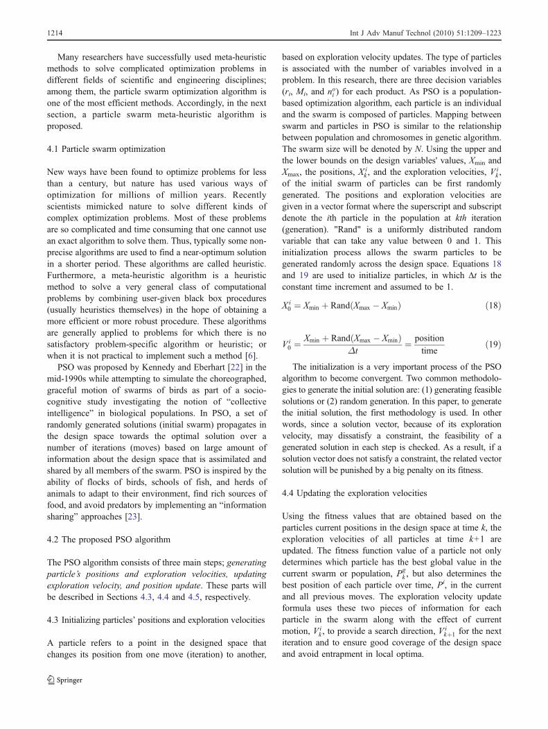
Many researchers have successfully used meta-heuristicmethods to solve complicated optimization problems indifferent fields of scientific and engineering disciplines;among them, the particle swarm optimization algorithm isone of the most efficient methods. Accordingly, in the nextsection, a particle swarm meta-heuristic algorithm isproposed.

4.1 Particle swarm optimization

New ways have been found to optimize problems for lessthan a century, but nature has used various ways ofoptimization for millions of million years. Recentlyscientists mimicked nature to solve different kinds ofcomplex optimization problems. Most of these problemsare so complicated and time consuming that one cannot usean exact algorithm to solve them. Thus, typically some non-precise algorithms are used to find a near-optimum solutionin a shorter period. These algorithms are called heuristic.Furthermore, a meta-heuristic algorithm is a heuristicmethod to solve a very general class of computationalproblems by combining user-given black box procedures(usually heuristics themselves) in the hope of obtaining amore efficient or more robust procedure. These algorithmsare generally applied to problems for which there is nosatisfactory problem-specific algorithm or heuristic; orwhen it is not practical to implement such a method [6].

PSO was proposed by Kennedy and Eberhart [22] in themid-1990s while attempting to simulate the choreographed,graceful motion of swarms of birds as part of a socio-cognitive study investigating the notion of “collectiveintelligence” in biological populations. In PSO, a set ofrandomly generated solutions (initial swarm) propagates inthe design space towards the optimal solution over anumber of iterations (moves) based on large amount ofinformation about the design space that is assimilated andshared by all members of the swarm. PSO is inspired by theability of flocks of birds, schools of fish, and herds ofanimals to adapt to their environment, find rich sources offood, and avoid predators by implementing an “informationsharing” approaches [23].

4.2 The proposed PSO algorithm

The PSO algorithm consists of three main steps; generatingparticle’s positions and exploration velocities, updatingexploration velocity, and position update. These parts willbe described in Sections 4.3, 4.4 and 4.5, respectively.

4.3 Initializing particles’ positions and exploration velocities

A particle refers to a point in the designed space thatchanges its position from one move (iteration) to another,

based on exploration velocity updates. The type of particlesis associated with the number of variables involved in aproblem. In this research, there are three decision variables(ri, Mi, and noi ) for each product. As PSO is a population-based optimization algorithm, each particle is an individualand the swarm is composed of particles. Mapping betweenswarm and particles in PSO is similar to the relationshipbetween population and chromosomes in genetic algorithm.The swarm size will be denoted by N. Using the upper andthe lower bounds on the design variables' values, Xmin andXmax, the positions, X i

k , and the exploration velocities, V ik ,

of the initial swarm of particles can be first randomlygenerated. The positions and exploration velocities aregiven in a vector format where the superscript and subscriptdenote the ith particle in the population at kth iteration(generation). "Rand" is a uniformly distributed randomvariable that can take any value between 0 and 1. Thisinitialization process allows the swarm particles to begenerated randomly across the design space. Equations 18and 19 are used to initialize particles, in which Δt is theconstant time increment and assumed to be 1.

X i0 ¼ Xmin þ Rand Xmax � Xminð Þ ð18Þ

V i0 ¼

Xmin þ Rand Xmax � Xminð ÞΔt

¼ position

timeð19Þ

The initialization is a very important process of the PSOalgorithm to become convergent. Two common methodolo-gies to generate the initial solution are: (1) generating feasiblesolutions or (2) random generation. In this paper, to generatethe initial solution, the first methodology is used. In otherwords, since a solution vector, because of its explorationvelocity, may dissatisfy a constraint, the feasibility of agenerated solution in each step is checked. As a result, if asolution vector does not satisfy a constraint, the related vectorsolution will be punished by a big penalty on its fitness.

4.4 Updating the exploration velocities

Using the fitness values that are obtained based on theparticles current positions in the design space at time k, theexploration velocities of all particles at time k+1 areupdated. The fitness function value of a particle not onlydetermines which particle has the best global value in thecurrent swarm or population, Pg

k , but also determines thebest position of each particle over time, Pi, in the currentand all previous moves. The exploration velocity updateformula uses these two pieces of information for eachparticle in the swarm along with the effect of currentmotion, V i

k , to provide a search direction, V ikþ1 for the next

iteration and to ensure good coverage of the design spaceand avoid entrapment in local optima.


The exploration velocity update formula includes somerandom parameters, rand, represented by the uniformlydistributed variables. The three values that affect the newsearch direction, namely, current motion, particle ownmemory, and swarm influence, are incorporated via a

summation approach as shown in Eq. 20 with three weightfactors, namely, inertia factor, w, self-confidence factor, C1,and swarm confidence factor, C2, respectively. The con-straint in Eq. 21 formed by Vmax, a maximum explorationvelocity, is specified to clamp the excessive accelerations.

ð20Þ

if V ikþ1 > Vmax

� �; V i

kþ1 ¼ Vmax

if V ikþ1 < �Vmax

� �; V i

kþ1 ¼ �Vmax

ð21ÞThe inertia weight w controls how much of the

previous exploration velocity should be retained from theprevious step. A larger inertia weight facilitates a global

No Yes

No

Yes

Stop

Set k=k+1

kk N=

Start

Initialize Position and

Set K=1

Set i=1 (i

( ) ( )iif X f P< i

iP X= ( )gkP Min P=

Calculate the Velocity of the

Calculate the Position of the Particle

Set i=i+1

i N=

YesNo

No Yes

No

Yes

Stop

Set

1k k= +

kk N=

No Yes

Start

Initialize Position and Velocity of the particles

Set k = 1

Set i = 1 (i indicates the number of the Particles)

( ) ( )iif X f P< i

iP X= ( )gkP Min P=

Calculate the Velocity of the Particle

Calculate the Position of the Particle

Set i = i + 1

i N=

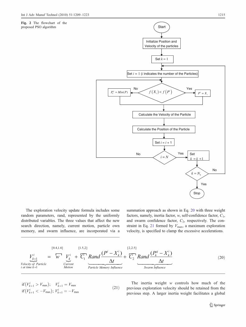
Fig. 2 The flowchart of theproposed PSO algorithm


search, while a smaller inertia weight facilitates a localsearch. A balance can be achieved between global andlocal exploration to speed up search results using adynamically adjustable inertia weight formulation. Intro-ducing a linearly decreasing inertia weight into theoriginal PSO significantly improves its performancethrough the parameter study of inertia weight [31, 37].The linear distribution of the inertia weight is expressed asfollows [31]:

w ¼ wmax � wmax � wmin

kmax� k ð22Þ

where, wmax and wmin are the initial and final values ofweighting coefficient, and kmax and k are the maximumiteration number and iteration counter, respectively. Therelated results of the two parameters wmax=0.9 and wmin=0.4 were investigated by Shi and Eberhart [37] and Nakaet al. [31].

Salman et al. [35] used the values of 0.9, 2, and 2 for w,C1 and C2 respectively, and suggested upper and lowerbounds on these values shown in Eq. 20. Other combinationsof the parameter values usually lead to much slowerconvergence or sometimes non-convergence at all. The tuningof the PSO algorithm weight factors is a topic that warrantsproper investigation but is outside the scope of this work.Meanwhile, according to some suggestions in the literature(see [31, 37]) in this research Eq. 22 for w is considered. Alsodifferent values for C1, C2 and N (population size) areconsidered and all possible combinations of them areexamined. Finally, the best combination of the parametersfrom all of the considered values in Table 3 is chosen.

4.5 Updating the position

Position update is the final step of a PSO-iteration andis performed using the current particle position and its

own updated exploration velocity vector shown inEq. 23.

X iKþ1 ¼ X i

K þ V iKþ1Δt ð23Þ

In short, the pseudo code of the proposed PSO algorithm is:

Initialize position (X0) and velocity of N particlesP1=X0

DO

k=1FOR i=1 to N particles

IF f (Xi)<f (Pi) THEN Pi=Xi

Calculate new velocity of the particleCalculate new position of particlePgk ¼ minðPÞ

END FORk ¼ k þ 1

UNTIL a sufficient good criterion is met.

Figure 2 shows the flowchart of the proposed algorithm.In the next section, a numerical example is given to

illustrate the application of the proposed PSO algorithm in areal world environment.

5 A numerical example

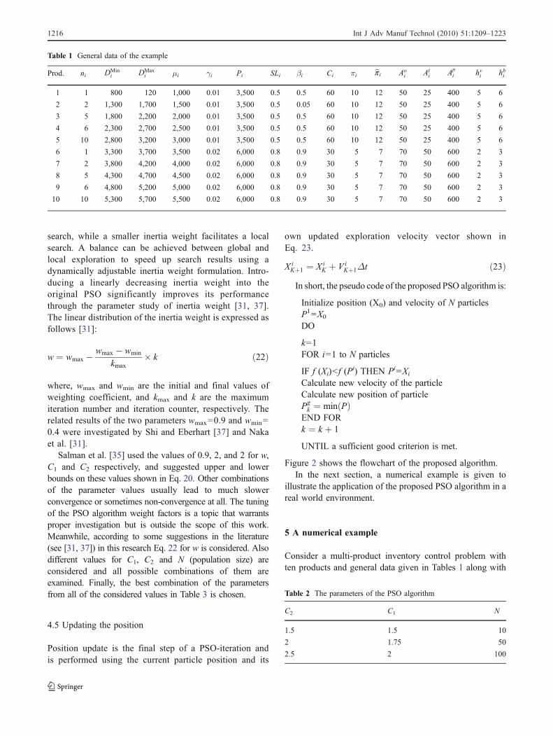
Consider a multi-product inventory control problem withten products and general data given in Tables 1 along with

Table 1 General data of the example

Prod. ni DMini DMax

i μi γi Pi SLi βi Ci πi bpi Aoi At

i Api hvi hbi

1 1 800 120 1,000 0.01 3,500 0.5 0.5 60 10 12 50 25 400 5 6

2 2 1,300 1,700 1,500 0.01 3,500 0.5 0.05 60 10 12 50 25 400 5 6

3 5 1,800 2,200 2,000 0.01 3,500 0.5 0.5 60 10 12 50 25 400 5 6

4 6 2,300 2,700 2,500 0.01 3,500 0.5 0.5 60 10 12 50 25 400 5 6

5 10 2,800 3,200 3,000 0.01 3,500 0.5 0.5 60 10 12 50 25 400 5 6

6 1 3,300 3,700 3,500 0.02 6,000 0.8 0.9 30 5 7 70 50 600 2 3

7 2 3,800 4,200 4,000 0.02 6,000 0.8 0.9 30 5 7 70 50 600 2 3

8 5 4,300 4,700 4,500 0.02 6,000 0.8 0.9 30 5 7 70 50 600 2 3

9 6 4,800 5,200 5,000 0.02 6,000 0.8 0.9 30 5 7 70 50 600 2 3

10 10 5,300 5,700 5,500 0.02 6,000 0.8 0.9 30 5 7 70 50 600 2 3

Table 2 The parameters of the PSO algorithm

C2 C1 N

1.5 1.5 10

2 1.75 50

2.5 2 100


TB=500,000. Each particle has 30 variables (three decisionvariables for each of the 10 products). Table 2 shows thedifferent values of the PSO parameters used to obtain thesolution. In this research, all of the possible combinations ofthe PSO parameters in Table 2 are employed and using themin (min) criterion, the best combination of the parametershas been selected. The best combination of the PSOparameters for this example is obtained as C1=C2=2, N=100.

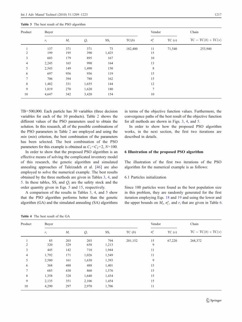
In order to show that the proposed PSO algorithm is aneffective means of solving the complicated inventory modelof this research, the genetic algorithm and simulatedannealing approaches of Taleizadeh et al. [46] are alsoemployed to solve the numerical example. The best resultsobtained by the three methods are given in Tables 3, 4, and5. In these tables, SSi and Qi are the safety stock and theorder quantity given in Eqs. 5 and 15, respectively.

A comparison of the results in Tables 3, 4, and 5 showthat the PSO algorithm performs better than the geneticalgorithm (GA) and the simulated annealing (SA) algorithms

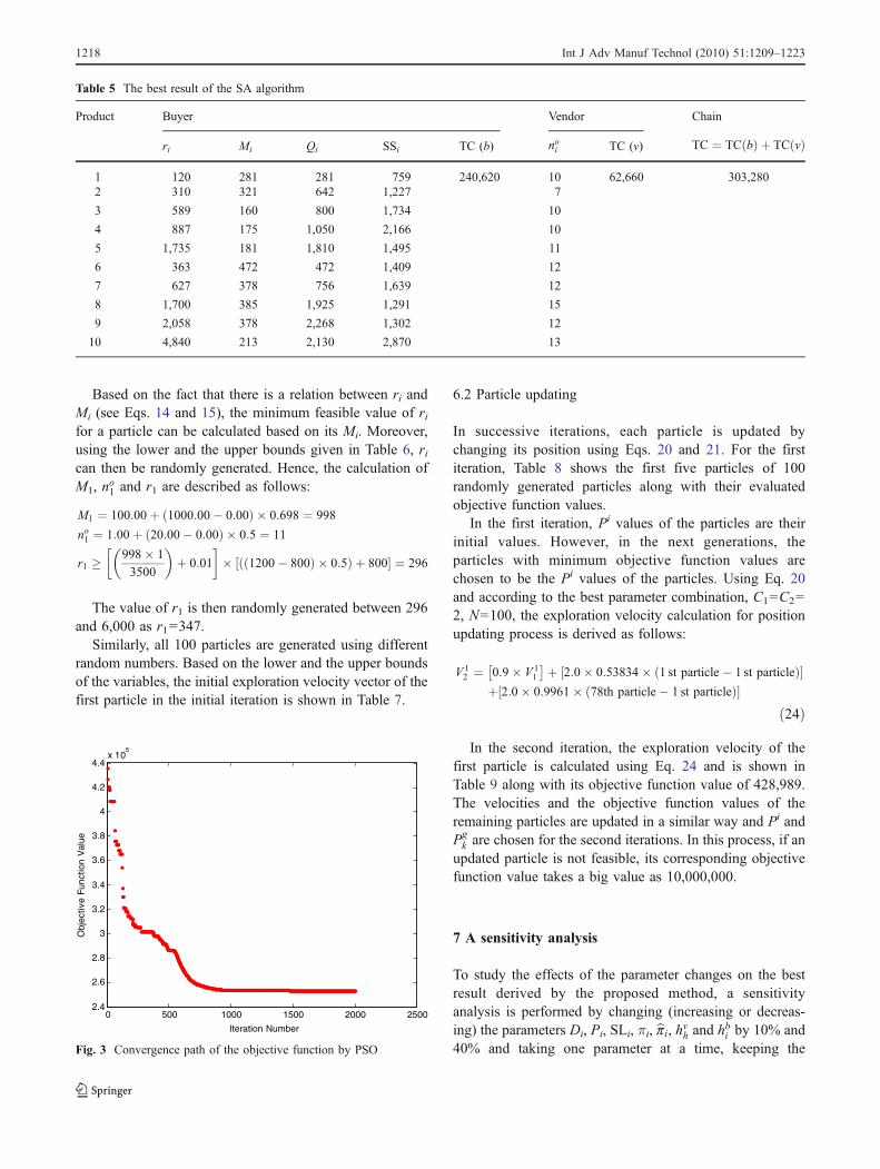
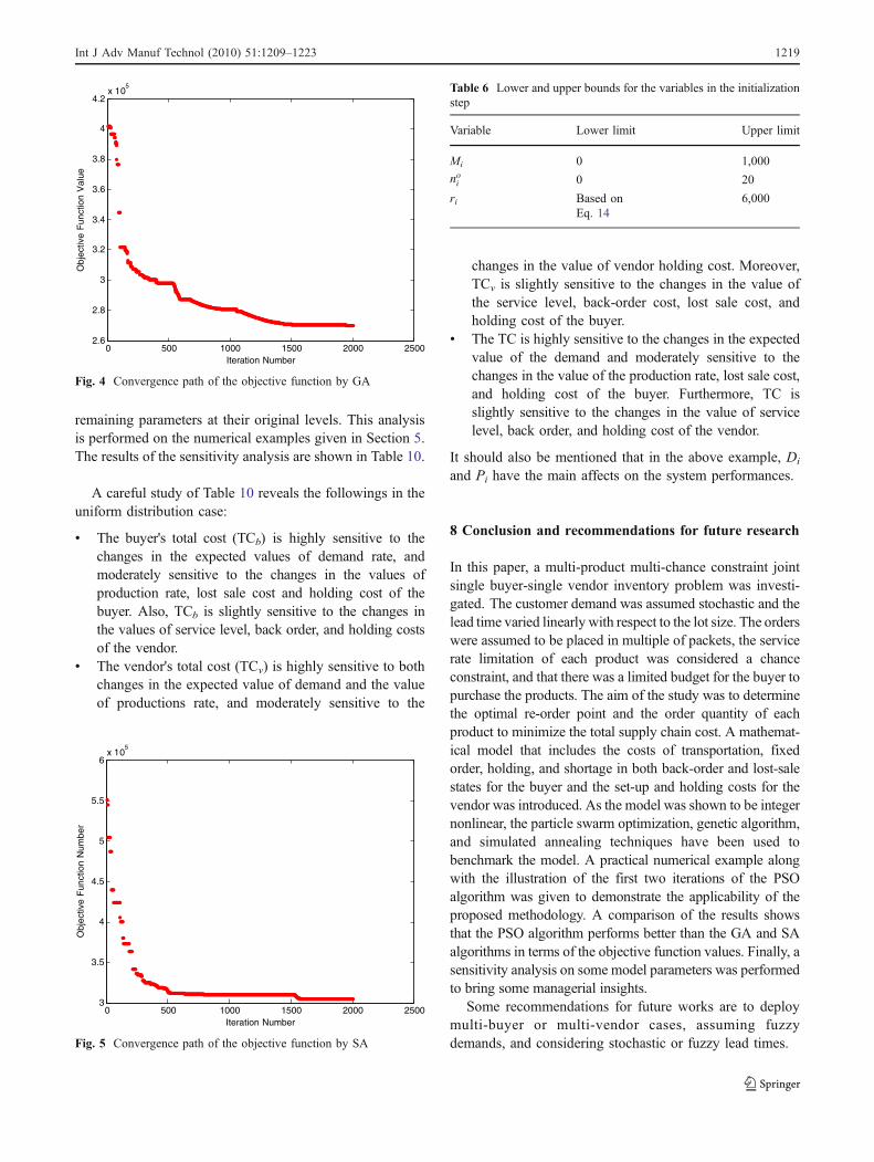
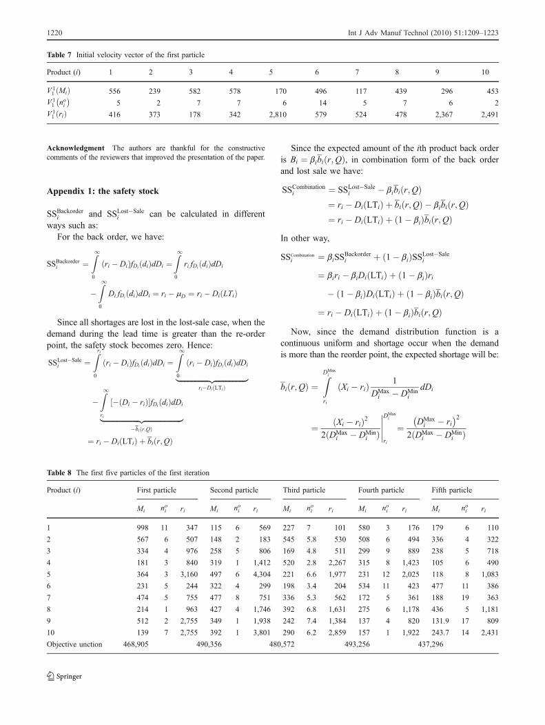
in terms of the objective function values. Furthermore, theconvergence paths of the best result of the objective functionfor all methods are shown in Figs. 3, 4, and 5.

In order to show how the proposed PSO algorithmworks, in the next section, the first two iterations aredescribed in details.

6 Illustration of the proposed PSO algorithm

The illustration of the first two iterations of the PSOalgorithm for the numerical example is as follows:

6.1 Particles initialization

Since 100 particles were found as the best population sizein this problem, they are randomly generated for the firstiteration employing Eqs. 18 and 19 and using the lower andthe upper bounds on Mi, noi , and ri that are given in Table 6.

Table 3 The best result of the PSO algorithm

Product Buyer Vendor Chain

ri Mi Qi SSi TC(b) noi TC (v) TC ¼ TCðbÞ þ TCðvÞ

1 137 371 371 73 182,400 11 71,540 253,9402 199 195 390 1,425 15

3 603 179 895 167 10

4 2,245 165 990 164 13

5 2,543 149 1,490 150 8

6 697 956 956 119 15

7 706 394 788 162 15

8 1,482 331 1,655 144 12

9 1,819 270 1,620 180 7

10 4,647 342 3,420 154 10

Table 4 The best result of the GA


ri Mi Qi SSi TC (b) noi TC (v) TC ¼ TCðbÞ þ TCðvÞ

1 85 203 203 794 201,152 15 67,220 268,3722 320 329 658 1,213 9

3 445 142 710 1,944 11

4 1,792 171 1,026 1,549 11

5 2,580 161 1,630 1,393 9

6 368 488 488 1,401 15

7 685 430 860 1,576 15

8 1,358 328 1,640 1,434 15

9 2,135 351 2,106 1,454 15

10 4,290 297 2,970 1,706 11


Based on the fact that there is a relation between ri andMi (see Eqs. 14 and 15), the minimum feasible value of rifor a particle can be calculated based on its Mi. Moreover,using the lower and the upper bounds given in Table 6, rican then be randomly generated. Hence, the calculation ofM1, no1 and r1 are described as follows:

M1 ¼ 100:00þ 1000:00� 0:00ð Þ � 0:698 ¼ 998

no1 ¼ 1:00þ 20:00� 0:00ð Þ � 0:5 ¼ 11

r1 � 998� 1

3500

� �þ 0:01

� �� 1200� 800ð Þ � 0:5ð Þ þ 800½ � ¼ 296

The value of r1 is then randomly generated between 296and 6,000 as r1=347.

Similarly, all 100 particles are generated using differentrandom numbers. Based on the lower and the upper boundsof the variables, the initial exploration velocity vector of thefirst particle in the initial iteration is shown in Table 7.

6.2 Particle updating

In successive iterations, each particle is updated bychanging its position using Eqs. 20 and 21. For the firstiteration, Table 8 shows the first five particles of 100randomly generated particles along with their evaluatedobjective function values.

In the first iteration, Pi values of the particles are theirinitial values. However, in the next generations, theparticles with minimum objective function values arechosen to be the Pi values of the particles. Using Eq. 20and according to the best parameter combination, C1=C2=2, N=100, the exploration velocity calculation for positionupdating process is derived as follows:

V 12 ¼ 0:9� V 1

1

�þ 2:0� 0:53834� 1 st particle � 1 st particleð Þ½ �þ 2:0� 0:9961� 78th particle � 1 st particleð Þ½ �

ð24Þ

In the second iteration, the exploration velocity of thefirst particle is calculated using Eq. 24 and is shown inTable 9 along with its objective function value of 428,989.The velocities and the objective function values of theremaining particles are updated in a similar way and Pi andPgk are chosen for the second iterations. In this process, if an

updated particle is not feasible, its corresponding objectivefunction value takes a big value as 10,000,000.

7 A sensitivity analysis

To study the effects of the parameter changes on the bestresult derived by the proposed method, a sensitivityanalysis is performed by changing (increasing or decreas-ing) the parameters Di, Pi, SLi, πi, bpi, hvh and hbi by 10% and40% and taking one parameter at a time, keeping the

0 500 1000 1500 2000 25002.4

2.6

2.8

3

3.2

3.4

3.6

3.8

4

4.2

4.4x 10

5

Iteration Number

Obj

ectiv

e Fu

nctio

n V

alue

Fig. 3 Convergence path of the objective function by PSO

Table 5 The best result of the SA algorithm


ri Mi Qi SSi TC (b) noi TC (v) TC ¼ TCðbÞ þ TCðvÞ

1 120 281 281 759 240,620 10 62,660 303,2802 310 321 642 1,227 7

3 589 160 800 1,734 10

4 887 175 1,050 2,166 10

5 1,735 181 1,810 1,495 11

6 363 472 472 1,409 12

7 627 378 756 1,639 12

8 1,700 385 1,925 1,291 15

9 2,058 378 2,268 1,302 12

10 4,840 213 2,130 2,870 13


remaining parameters at their original levels. This analysisis performed on the numerical examples given in Section 5.The results of the sensitivity analysis are shown in Table 10.

A careful study of Table 10 reveals the followings in theuniform distribution case:

& The buyer's total cost (TCb) is highly sensitive to thechanges in the expected values of demand rate, andmoderately sensitive to the changes in the values ofproduction rate, lost sale cost and holding cost of thebuyer. Also, TCb is slightly sensitive to the changes inthe values of service level, back order, and holding costsof the vendor.

& The vendor's total cost (TCv) is highly sensitive to bothchanges in the expected value of demand and the valueof productions rate, and moderately sensitive to the

changes in the value of vendor holding cost. Moreover,TCv is slightly sensitive to the changes in the value ofthe service level, back-order cost, lost sale cost, andholding cost of the buyer.

& The TC is highly sensitive to the changes in the expectedvalue of the demand and moderately sensitive to thechanges in the value of the production rate, lost sale cost,and holding cost of the buyer. Furthermore, TC isslightly sensitive to the changes in the value of servicelevel, back order, and holding cost of the vendor.

It should also be mentioned that in the above example, Di

and Pi have the main affects on the system performances.

8 Conclusion and recommendations for future research

In this paper, a multi-product multi-chance constraint jointsingle buyer-single vendor inventory problem was investi-gated. The customer demand was assumed stochastic and thelead time varied linearly with respect to the lot size. The orderswere assumed to be placed in multiple of packets, the servicerate limitation of each product was considered a chanceconstraint, and that there was a limited budget for the buyer topurchase the products. The aim of the study was to determinethe optimal re-order point and the order quantity of eachproduct to minimize the total supply chain cost. A mathemat-ical model that includes the costs of transportation, fixedorder, holding, and shortage in both back-order and lost-salestates for the buyer and the set-up and holding costs for thevendor was introduced. As the model was shown to be integernonlinear, the particle swarm optimization, genetic algorithm,and simulated annealing techniques have been used tobenchmark the model. A practical numerical example alongwith the illustration of the first two iterations of the PSOalgorithm was given to demonstrate the applicability of theproposed methodology. A comparison of the results showsthat the PSO algorithm performs better than the GA and SAalgorithms in terms of the objective function values. Finally, asensitivity analysis on some model parameters was performedto bring some managerial insights.

Some recommendations for future works are to deploymulti-buyer or multi-vendor cases, assuming fuzzydemands, and considering stochastic or fuzzy lead times.

Table 6 Lower and upper bounds for the variables in the initializationstep

Variable Lower limit Upper limit

Mi 0 1,000

noi 0 20

ri Based onEq. 14

6,000

0 500 1000 1500 2000 25003

3.5

4

4.5

5

5.5

6x 10

5

Iteration Number

Obj

ectiv

e F

unct

ion

Num

ber

Fig. 5 Convergence path of the objective function by SA

0 500 1000 1500 2000 25002.6

2.8

3

3.2

3.4

3.6

3.8

4

4.2x 10

5

Iteration Number

Obj

ectiv

e F

unct

ion

Val

ue

Fig. 4 Convergence path of the objective function by GA


Acknowledgment The authors are thankful for the constructivecomments of the reviewers that improved the presentation of the paper.

Appendix 1: the safety stock

SSBackorderi and SSLost�Salei can be calculated in different

ways such as:For the back order, we have:

SSBackorderi ¼Z10

ri � Dið ÞfDi dið ÞdDi ¼Z10

ri fDi dið ÞdDi

�Z10

Di fDi dið ÞdDi ¼ ri � mD ¼ ri � Di LTið Þ

Since all shortages are lost in the lost-sale case, when thedemand during the lead time is greater than the re-orderpoint, the safety stock becomes zero. Hence:

SSLost�Salei ¼

Zri0

ri � Dið ÞfDi dið ÞdDi ¼Z10

ri � Dið ÞfDi dið ÞdDi|fflfflfflfflfflfflfflfflfflfflfflfflfflfflfflfflffl{zfflfflfflfflfflfflfflfflfflfflfflfflfflfflfflfflffl}ri�Di LTið Þ

�Z1ri

� Di � rið Þ½ �fDi dið ÞdDi

|fflfflfflfflfflfflfflfflfflfflfflfflfflfflfflfflfflfflfflfflffl{zfflfflfflfflfflfflfflfflfflfflfflfflfflfflfflfflfflfflfflfflffl}�bi r;Qð Þ

¼ ri � Di LTið Þ þ bi r;Qð Þ

Since the expected amount of the ith product back orderis Bi ¼ bibi r;Qð Þ, in combination form of the back orderand lost sale we have:

SSCombinationi ¼ SSLost�Sale

i � bibi r;Qð Þ¼ ri � Di LTið Þ þ bi r;Qð Þ � bibi r;Qð Þ¼ ri � Di LTið Þ þ 1� bið Þbi r;Qð Þ

In other way,

SSCombinationi ¼ biSS

Backorderi þ 1� bið ÞSSLost�Sale

i

¼ biri � biDi LTið Þ þ 1� bið Þri� 1� bið ÞDi LTið Þ þ 1� bið Þbi r;Qð Þ

¼ ri � Di LTið Þ þ 1� bið Þbi r;Qð ÞNow, since the demand distribution function is a

continuous uniform and shortage occur when the demandis more than the reorder point, the expected shortage will be:

bi r;Qð Þ ¼ZDMax

i

ri

Xi � rið Þ 1

DMaxi � DMin

i

dDi

¼ Xi � rið Þ22 DMax

i � DMinið Þ

DMax

i

ri

¼ DMaxi � ri

� �22 DMax

i � DMinið Þ

Table 7 Initial velocity vector of the first particle

Product (i) 1 2 3 4 5 6 7 8 9 10

V 11 Mið Þ 556 239 582 578 170 496 117 439 296 453

V 11 noi� �

5 2 7 7 6 14 5 7 6 2

V 11 rið Þ 416 373 178 342 2,810 579 524 478 2,367 2,491

Table 8 The first five particles of the first iteration

Product (i) First particle Second particle Third particle Fourth particle Fifth particle

Mi noi ri Mi noi ri Mi noi ri Mi noi ri Mi noi ri

1 998 11 347 115 6 569 227 7 101 580 3 176 179 6 110

2 567 6 507 148 2 183 545 5.8 530 508 6 494 336 4 322

3 334 4 976 258 5 806 169 4.8 511 299 9 889 238 5 718

4 181 3 840 319 1 1,412 520 2.8 2,267 315 8 1,423 105 6 490

5 364 3 3,160 497 6 4,304 221 6.6 1,977 231 12 2,025 118 8 1,083

6 231 5 244 322 4 299 198 3.4 204 534 11 423 477 11 386

7 474 5 755 477 8 751 336 5.3 562 172 5 361 188 19 363

8 214 1 963 427 4 1,746 392 6.8 1,631 275 6 1,178 436 5 1,181

9 512 2 2,755 349 1 1,938 242 7.4 1,384 137 4 820 131.9 17 809

10 139 7 2,755 392 1 3,801 290 6.2 2,859 157 1 1,922 243.7 14 2,431

Objective unction 468,905 490,356 480,572 493,256 437,296


Finally, knowing that LTi ¼ Qi

Piþ gi

� we have:

SSi ¼ ri � DiQi

Piþ gi


i � ri� �2

2 DMaxi � DMin

ið Þ

Appendix 2: the buyer back order and lost sale costs

According to Appendix (1), we have:

bi r;Qð Þ ¼ DMaxi � ri

� �22 DMax

i � DMinið Þ

Knowing that:

Bi ¼ biDi

noi Qibi r;Qð Þ ¼ bi

Di

noi Qi

DMaxi � ri

� �22 DMax

i � DMinið Þ

Li ¼ 1� bið Þ Di

noi Qibi r;Qð Þ ¼ 1� bið Þ Di

noi Qi

DMaxi � ri

� �22 DMax

i � DMinið Þ

The expected costs of back order and lost sale based onthe expressions for πi and bpi are:CBb ¼

pibiDi DMaxi � ri


i � DMinið Þ

CLb ¼bpi 1� bið ÞDi DMax

i � ri� �2


ið Þ

Appendix 3: service rate as a chance constraint

Knowing that if X∼U [a, b] then Y ¼ KX � U Ka;Kb½ �, thedistribution function of Di(LTi) is uniform on LTið ÞDMax

i ;

LTið ÞDMini �. Since the shortages of the ith product only

occur when the demand during the lead time is more thanthe reorder point and the lower limit for the service level isSLi, then:

P Di LTið Þ � rið Þ � SLi

)Zri

LTi DMinið Þ

1

LTi DMaxi � DMin

ið Þdi � SLi

) ri � LTi DMini

� �LTi DMax

i � DMinið Þ � SLi

) ri � LTi DMaxi � DMin

i

� �SLi þ LTi D

Mini

� �) ri � LTi DMax

i � DMini

� �SLi þ DMin

i

� � �) ri � Qi

Piþ gi

� �DMax

i � DMini

� �SLi þ DMin

i

� � �

Table 9 The first particle of the second iteration

First particle 1 2 3 4 5 6 7 8 9 10

Mi 757 1,148 904 575 606 1,501 782 1,399 640 918

noi 6 4 11 8 6 3 14 15 12 7

ri 585 1,115 2,102 1,533 3,010 1,274 1,217 4,844 2,328 5,978

Table 10 The results of the sensitivity analysis

Parameters %Changes

% Changes in

TC (b) TC (v) TC

Di +40 +80 −84 +39

+10 +30 −19 +16

−10 −16 −6 −13−40 −50 −39 −47

Pi +40 +10 +31 +16

+10 +17 +8 +15

−10 +11 −31 −0.65−40 Infeasible Infeasible Infeasible

SLi +40 −4 −4 −4+10 +15 −3 +10

−10 +8 +5 +7

−40 +7 −3 +4

πi +40 +6 +2 +4

+10 −1 +1 −0.3−10 −7 −1 −5−40 −12 −10 −12

p̂i +40 +18 −0.7 +12

+10 +5 −0.5 +2

−10 −12 −2 −9−40 −16 −11 −13

hvi +40 +6 +27 +10

+10 +3 +12 +7

−10 −3 −10 −2−40 −5 −22 −5

hbi +40 +25 +3 +19

+10 +7 +0.3 +4

−10 −3 −3 −3−40 −29 −2 −22


References

1. Aarts EHL, Korst JHM (1989) Simulated annealing and Boltz-mann machine; a stochastic approach to computing, 1st edn.Wiley, Chichester, UK

2. Al-Tabtabai H, Alex AP (1999) Using genetic algorithms tosolve optimization problems in construction. Eng Con Arch Man6:121–132

3. Banerjee A (1986) A joint economic lot size model for purchaserand vendor. Decis Sci 17:292–311

4. Ben-Daya M, Raouf A (1994) Inventory models involving leadtime as a decision variable. Journal of the Operational ResearchSociety 45:579–582

5. Ben-Daya M, Hariga M (2004) Integrated single vendor singlebuyer model with stochastic demand and variable lead time. Int JProd Econ 92:75–80

6. Dorigo M, Stutzle T (2004) Ant colony optimization. MIT Press,Cambridge

7. Dueck G, Scheuer T (1990) Threshold accepting: a generalpurpose algorithm appearing superior to simulated annealing. JComput Phys 90:161–175

8. El-Sharkawi L (2008) Modern heuristic optimization techniques,1st edn. Wiley Inter Science, New Jersey

9. Gaiduk AR, Vershinin YA, West MJ (2002) Neural networks andoptimization problems. In Proceedings of IEEE 2002 InternationalConference on Control Applications, 1:37–41

10. Geem ZW, Kim JH, Loganathan GV (2001) A new heuristicoptimization algorithm: harmony search. Simulation 76:60–68

11. Gen M, Cheng R (1997) Genetic algorithm and engineeringdesign, 1st edn. Wiley, New York

12. Goyal SK (1988) Joint economic lot size model for purchaser andvendor: a comment. Decis Sci 19:236–241

13. Goyal SK, Gupta YP (1989) Integrated inventory models: thevendor–buyer coordination. Eur J Oper Res 41:261–269

14. Guo YW, Li WD, Mileham AR, Owen GW (2008) Optimizationof integrated process planning and scheduling using a particleswarm optimization approach. Int J Prod Res 40:1–22

15. Hadley G, Whitin TM (1963) Analysis of inventory systems.Prentice-Hall, Englewood Cliffs

16. Hariga M, Ben-Daya M (1999) Some stochastic inventorymodels with deterministic variable lead time. Eur J Oper Res113:42–51

17. Heydari J, Baradaran-Kazemzadeh R, Chaharsooghi SK (2009) Astudy of lead time variation impact on supply chain performance.Int J Adv Manuf Technol 40:1206–1215

18. Hill R (1999) The optimal production and shipment policy for thesingle-vendor single-buyer integrated production–inventory prob-lem. Int J Prod Res 37:2463–2475

19. Hsiao JM, Lin C (2005) A buyer-vendor EOQ model withchangeable lead time in supply chain. Int J Adv Manuf Technol26:917–921

20. Joo SJ, Bong JY (1996) Construction of exact D-optimal designsby Tabu search. Comput Stat Data Anal 21:181–191

21. Kannan G, Noorul-Haq A, Devik M (2009) Analysis of closedloop supply chain using genetic algorithm and particle swarmoptimization. Int J of Prod Res 47:1175–1200

22. Kennedy J, Eberhart R (1995) Particle swarm optimization.Proceedings of the IEEE International Conference on NeuralNetworks, Perth, Australia, 1942–1945

23. Kennedy J, Eberhart R (2001) Swarm intelligence. Academic, SanDiego

24. Kim CO, Jun J, Baek JK, Smith RL, Kim YD (2005) Adaptiveinventory control models for supply chain management. Int J AdvManuf Technol 26:1184–1192

25. Laumanns M, Thiele L, Deb K, Zitzler E (2002) Combiningconvergence and diversity in evolutionary multi-objective optimi-zation. Evol Comput 10:263–282

26. Lee KS, Geem ZW (2004) A new structural optimization methodbased on the harmony search algorithm. Comput Struct 82:781–798

27. Liu B, Wang L, Jin Y (2008) An effective hybrid PSO-basedalgorithm for flow shop scheduling with limited buffers. ComputOper Res 35:2791–2806

28. Liu B (2004) Uncertainty theory: an introduction to its axiomaticfoundations. Springer, Berlin

29. Lodree E, Jang W, Klein CM (2004) Minimizing response time ina two-stage supply chain system with variable lead time andstochastic demand. Int J of Prod Res 42:2263–2278

30. Lu L (1995) A one-vendor multi-buyer integrated inventorymodel. Eur J Oper Res 81:312–323

31. Naka S, Genji T, Yura T, Fukuyama Y (2001) Practical distributionstate estimation using hybrid particle swarm optimization. Proceed-ings of the IEEE Power Engineering Society Winter Meeting

32. Ouyang LY, Yeh NC, Wu KS (1996) Mixture inventory modelswith backorders and lost sales for variable lead time. J Oper ResSoc 47:829–832

33. Ouyang LY, Chuang BR (2000) A periodic review inventorymodel involving variable lead time with a service level constraint.Int J Sys Sci 31:1209–1215

34. Rahimi-Vahed AR, Mirghorbani SM, Rabbani M (2007) A hybridmulti-objective particle swarm algorithm for a mixed-modelassembly line sequencing problem. Eng Optim 39:877–898

35. Salman A, Ahmad I, Al-Madani S (2003) Particle swarmoptimization for fast assignment problem. Microprocess Microsyst26:363–371

36. Sha DY, Hsu C (2008) A new particle swarm optimization forthe open shop scheduling problem. Comput Oper Res 35:3243–3261

37. Shi Y, Eberhart RC (1999) Empirical study of particle swarmoptimization. Proceedings of the 1999 Congress on EvolutionaryComputation, 1945–1950

38. Siajadi H, Ibrahim RN, Lochert PB (2006) A single-vendormultiple-buyer inventory model with a multiple-shipment policy.Int J Adv Manuf Technol 27:1030–1037

39. Su S, Zhan D, Xu X (2008) An extended state task networkformulation for integrated production-distribution planning insupply chain. Int J Adv Manuf Technol 37:1232–1249

40. Taleizadeh AA, Aryanezhad MB, Niaki STA (2008) Optimizingmulti-product multi-constraint inventory control systems withstochastic replenishment. J Appl Sci 8:1228–1234

41. Taleizadeh AA, Niaki STA, Hosseini V (2008) The multi-productmulti-constraint newsboy problem with incremental discount andbatch order. As J Appl Sci 1:110–122

42. Taleizadeh AA, Moghadasi H, Niaki STA, Eftekhari A (2008) AnEOQ-joint replenishment policy to supply expensive imported rawmaterials with payment in advance. J Appl Sci 8:4263–4273

43. Taleizadeh AA, Niaki STA, Aryanezhad MB (2009) Multi-product multi-constraint inventory control systems with stochasticreplenishment and discount under fuzzy purchasing price andholding costs. Am J Appl Sci 6:1–12

44. Taleizadeh AA, Niaki STA, Hosseini V (2009) Optimizing multi-product multi-constraint bi-objective newsboy problem withdiscount by a hybrid method of goal programming and geneticalgorithm. Eng Optim 41:437–457

45. Taleizadeh AA, Niaki STA, Aryanezhad MB (2009) A hybridmethod of Pareto, TOPSIS and genetic algorithm to optimizemulti-product multi-constraint inventory systems with randomfuzzy replenishment. Math Comput Model 49:1044–1057

46. Taleizadeh AA, Niaki STA, Aryanezhad MB (2009d) Multi-product multi-constraint inventory control systems with stochastic


period length and total discount under fuzzy purchasing price andholding costs. Int J Sys Sci (in press)

47. Wang YC (2008) Evaluating flexibility on order quantity and deliverylead time for a supply chain system. Int J Sys Sci 39:1193–1202

48. Wee HM, Yang PC (2007) A mutual beneficial pricing strategy ofan integrated vendor-buyers inventory system. Int J Adv ManufTechnol 34:179–187

49. Wu KS (2001) A mixed inventory model with variable lead timeand random supplier capacity. Prod Plan Control 12:353–361

50. Yapicioglu H, Smith AE, Dozier G (2007) Solving the semi-desirable facility location problem using bi-objective particleswarm. Eur J Oper Res 177:733–749

51. Zahara E, Hu CH (2008) Solving constrained optimizationproblems with hybrid particle swarm optimization. Eng Optim40:1031–1049

52. Zequeira RI, Durn A, Gutirrez G (2005) A mixed inventory modelwith variable lead time and random back-order rate. Int J Sys Sci36:329–339


Documents

A particle swarm optimization approach for constraint ...niadr/PUBLICATIONS/LIACC_publications... · ORIGINAL ARTICLE A particle swarm optimization approach for constraint joint single