Embed Size (px)
Citation preview

AD-A008 985
EFFECT OF SPEED ON TIRE-SOIL INTERACTIONAND DEVELOPMENT OF TOWED PNEUMATICTIRE-SOIL MODEL
Leslie L. Karafiath, et al
Grumman Aerospace Corporation
Prepared for:
Army Tank-Automotive Command
October 1974
DISTRIBUTED BY:
National Technical Information ServiceU. S. DEPARTMENT OF COMMERCE
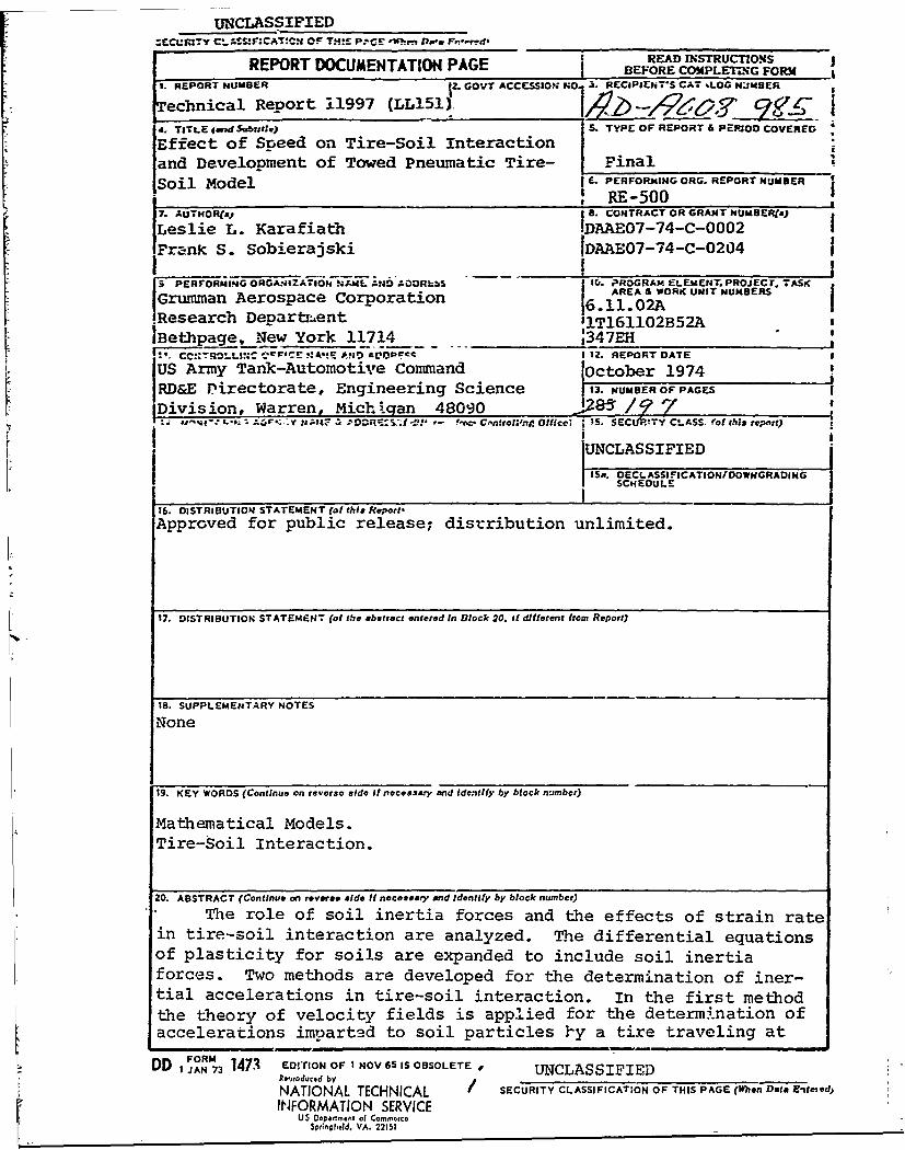
UNCLASSIFIED.ZECUFUITYCL C F-- :CATC!I OF TM!.SP-CGE w%.e DaF, ,-.
REPORT DOCUMENTATIONt PAGE 9 READ INSTRUCrIonS JRMPBEFORE COMPLETING FORM
I. REPORT NUMBER 1Z. GOVT ACCESSION NO 3. RECIPIENT°S CAT %LOG NUMBER
Technical Report 11997 (LL151). I zeS $
4. TITLE (adrub Iti) S. TYPE OF REPORT 6 PER OD COVERED
Effect of Speed on Tire-Soil Interactionand Development of Towed Pneumatic Tire- FinalSoil Model PERFORMING ORG. REPORT NJMERRE-500i7. AUTHOR(sj
a. CONTRACT OR GRANT NUMBER(a)
Leslie L. Karafiath IDAAE07-74-C-0002Frank S. Sobierajski IDAAE07-74-C-0204z 4
PERFORMING ORGAIZAT-ION NAML AND AODRL5S 11. PROGRAM ELEMENT. PROJECT.T ASI
AREA 5 WORK UNIT NUMBERSGrumman Aerospace Cororation 6.ll.02AResearch Departr:ent 'IT161102B52A
IBethpage, New York 11714 ___ ;347EH:'. CC*': ROL'LI ;*'r C CaiAE nA*1C AVOP£P 1 12. REPORT DATE
US Army Tank-Automotive Command October 1974RD&E Pirectorate, Engineering Science 13. NUMBER OF PAGES
Division, Warren, Michigan 48090 I285/ '7:.; l' L,; %,%V% .y NA4 a';i8 PO-DR;e'- . * , - O., C .n1rol'nA. Office) 1 15. SECU ?. TY CLASS- 'Of t.his report)
UNCLASSIFIED15jr. DECLASSI FICATION/DOWNGRADING
SCHEDULE
16. DISTRIBUTION STATEMENT (of this Repot-Approved for public release; distribution unlimited.
17. DISTRIBUTION STATEMENHT (of the abstract entered in Block 20. it different from Report)
18. SUPPLEMENTARY NOTES
None
19. KEY WORDS (Continue on reverse side it necessary and Identify by block number)
Mathematical Models.Tire-Soil Interaction.
20. ABSTRACT (Continua on reverse aide If noceeaaty and identify by block number)
The role of soil inertia forces and the effects of strain rate
in tire-soil interaction are analyzed. The differential equationsof plasticity for soils are expanded to include soil inertiaforces. Two methods are developed for the determination of iner-tial accelerations in tire-soil interaction. In the first method
the theory of velocity fields is applied for the determination ofaccelerations impartsd to soil particles 1-y a tire traveling at
DD I ANR3 147. EDTrION OF I NOV65 IS OBSOLETE UNCLASSIFIEDRks,,rodchild by ______________________________
NATIONAL TECHNICAL / SECURITY CLASSIFICATION OF THIS PAGE (When Data E-iteted
INFORMATION SERVICEU$ Depaiient of Commerco
Spingheld, VA. 22151

UNCLASSIFIEDSECURITY CLASSIFICATION OF THIS PAGC(fm Dtae afmd)
* constant velocity. An iterative scheme is developed that succes-sively updates the geometry of slip line field-- for velocityincrements and associated inertia forces. In the second methodsoil particle accelerations are computed on the basis of particle
*path geometry. An analytical form of the particle path is assumedand related to the time events of tire travel. Computations byboth methods indicate that the solution of the differential equa-tions of plasticity for soil becomes multivalued at a relativelylow travel velocity. Up to this velocity, tire-soil interaction isnot significantly affected by soil inertia forces. Beyond thisvelocity the multivaluedness of solutions of the differential equa-tions indicates a condition that has not been explored yet for itseffect on soil behavior and cannot be treated by present theories.
The effect of strain rate of soil strength properties isanalyzed and recognized as the major contributor to the improve-ment of tire performance with speed.
A mathematical model for towed pneumatic tires and soil isdeveloped for the simulation of towed tire-soil interaction. Towedforce coefficient predictions are compared with experimentalresults.
/6L. UNCLASSIFIEDSECURITY CLASSIFICATION OF THIS PAGE(Whn Data Enterd)

RE- 500
EFFECT OF SPEED ON TIRE-SOIL INTERACTION*
AND
DEVELOPMENT OF TOWED PNEUMATIC TIRE-SOIL MODEL
* .by
Leslie L. Karafiath
and
Frank S. Sobierajski
- Prepared Under Contracts
" "DAAE07-74-C-0002 and DAAE07-74-C-0204
for
United States Army Tank-Automotive CommandWarren, Michigan
by
Research DepartmentGrumman Aerospace CorporationBethpage, New York 11714
October 1974
, Approved by:Charles E. Mack, Jr.
'// Director of Research

FOREWORD
Simulating the interaction of terrain, vehicle, and man is
essential to improving land mobility technology - a goal of the
U.S. Army Tank-Automotive Command (TACOM) and the U.S. Army Corps
f "of Engineers Waterways Experiment Station (WES). Under TACOM con-
tract, Grumman has been actively supporting this effort and com-
- p" pleted the development of a first generation mathematical model
for driven rigid wheel and pneumatic tire-soil interaction.
F- This model, conceived as an alternate submodel in the terrain-
vehicle-man simulation, called the AMC Vehicle Mobility Model,
f" allows the computation of tire performance in both purely fric-
tional or cohesive and frictional-cohesive soils.
This first generation mathematical model is based on the con-
cept of "steady state" in the soil that assumes a low and constant
velocity of travel. Obsezvations in the laboratory and in the
field indicate that tire performance improves with travel velocity
under certain conditions.
To take this factor into account in mobility evaluation and
take advantage of it in off-road vehicle development it is neces-
sary to analyze the effects of soil inertia and loading rates on
-tire-soil interaction. In a follow-on program to the development
of a first generation pneumatic tire-soil model, the results of
which are presented in this program, the model was expanded to in-
7 clude soil inertia forces. The effects of the loading rate were
anialyzed by adjusting the strength properties of soil for the
strain rate corresponding to the travel velocity of the tire. The
expanded model was also shown to be suitable for the determination
of spring constants that can be applied in vehicle dynamic models.
" iii

For the analyses of cross country mobility of trailer-mountedweapons, a towed tire-soil model is needed that predicts the motionresistance and sinkage of towed pneumatic tires. The basic con-cepts of tire-soil interaction were applied to the case of towedtire and an appropriate model, described in the second part ofthis report, has been developed.
iv

rc ABSTRACT
The role of soil inertia forces and the effects of strain rate
f in tire-soil interaction are analyzed. The differential equations
of plasticity for soils are expanded to include soil inertia
*forces. Two methods are developed for the determination of iner-
tial accelerations in tire-soil interaction. In the first method
the theory of velocity fields is applied for the determination of
accelerations imparted to soil particles by a tire traveling at
" - constant velocity. An iterative scheme is developed that succes-
sively updates the geometry of slip line fields for velocity in-
crements and associated inertia forces. In the second method soil
particle accelerations are computed on the basis of particle path
geometry. An analytical form of the particle path is assumed and
related to the time events of tire travel. Computations by both
methods indicate that the solution of the differential equations
of plasticity for soil becomes multivalued at a relatively low~travel velocity. Up to this velocity tire-soil interaction is not
significantly affected by soil inertia forces. Beyond this veloc-
ity the multivaluedness of solutions of the differential equations
indicates a condition that has not been explored yet for its effect
on soil behavior and cannot be treated by present theories.
The effect of strain rate of soil strength properties is ana-
lyzed and recognized as the major contributor to the improvement
A. of tire performance-with speed.
A mathematical model for towed pneumatic tires and soil is de-
veloped for the simulation of towed tire-soil interaction. Towed
- force coefficient predictions are compared with experimental re-
* sults.
v

IL
ACKNOWLEDGMENT
The work reported herein was performed for the Mobility Sys-
tems Laboratory of the U.S. Army Tank-Automotive Command (TACOM),
Warren, Michigan, under the general supervision of Dr. Jack G.
Parks, Chief of the Engineering Science Division and Mr. Zoltan J.
Janosi, Supervisor, Research and Methodology Function. Mr. Zoltan
J. Janosi was also technical monitor. Their help and valuablesuggestions in carrying out this work are gratefully acknowledged.
In the development of the towed tire-soil model use was made
of computer techniques, developed in an independent research pro-
gram, that allows running of large programs on minicomputers. Ac-
knowledgment is due to Mr. R. McGill, head of the Grumman Research
I Department's Computer Sciences Group, who made the necessary pro-
visions in the program for its accommodation on the minicomputer.
Wig
vi Preceding page blank

TABLE OF CONTENTS
Section Page
I Scope of Work ................................ I
II Effect of Speed on Tire-Soil Interaction 3
III Effect of Soil Inertia Forces on Tire-SoilInteraction .................................. 5
IV Determination of Soil Inertia Forces by the
Theory of Velocity Fields .................... 7
Theoretical Background .................. 7
Kinematic Boundary Conditions ........... 12
Computation of Inertial Accelerationsfrom Velocity Fields .................... 23
Computational Scheme for the Considerationof Soil Inertia Forces in Tire-SoilInteraction ............................. 24
Problems Encountered with Developme.tof the Computer Program ................. 24
Results of Sample Computations .......... 30
Summary Discussion of the Method of
Velocity Fields and Conclusions ......... 31
V Determination of Soil Inertia Forces by theParticle Path Method .......................... 35
Introduction ............................. 35
Experimental Information on ParticlePath Geometry ........................... 35
Idealization of Particle Path Geometry 37
Al Use of the Idealized Particle Path
Geometry in the Tire-Soil Model ......... 47
Problems Encountered with the Developmentof the Computer Program ................. 48
Results of Sample Computations .......... 48
Summary Discussion of the Particle Path
Method and Conclusions .................. 50
Preceding page blank

i
Section Page
VI Effect of Loading Rate on Soil Strengthand Tire-Soil Interaction ..................... 53
Introduction ............................. 53
Physical Causes of Strain Rate DependentStrength Properties of Soils ............ 54
Correlation of Strain-Rate Effects inLaboratory and Field Tests for StrengthProperty Determination and in Tire-SoilInteraction ............................. 57
Consideration of Strain Rate Effects inthe Tire-Soil Model ...................... 60
Summary Discussion of the Effects ofStrain Rate on Tire-Soil Interactionand Conclusions ......................... 64
VII Use of Tire-Soil Model in Vehicle RideDynamics Simulation .......................... 67
VIII Towed Pneumatic Tire-Soil Model.............. 73
Introduction ............................ 73
Experimental Information on TowedPneumatic Tire Behavior ................. 73
Concept of Towed Tire-Soil Interaction .. 76
Development of Towed Tire-Soil Model .... 77
Problems Encountered ..................... 79
Results of the Analyses of ExperimentalData .................................... 81
Evaluation of the Towed Tire-SoilModel ................................... 90
IX Conclusions and Recommendations .............. 95
X References ................................... 99
Appendices
Appendix A - Computer Program Flow Chart for Analysisof Effect of Soil Inertia Forces on TirePerformance by Method of VelocityFields ................................. A-1
x

Section Page
Appendix B - Computer Program Chart for Computation3- of Tire Performance with Consideration
of Inertia Forces by Particle PathMethod ............................... B-1
Appendix C - Computer Program Flow Chart forComputation of Towed Force Coefficientsfor Pneumatic Tires ..................... C-I
Distribution List
DD Form 1473
Ix i4. xi

LIST OF ILLUSTRATIONS
Figure Page
1 Velocity Vectors along Characteristic Lines .... l
2 Boundaries of a Slip Line Field in Tire-SoilInteraction Problems ........................... 11
3 Trajectory of a Point at the Circumference ofa Deformable Tire............................. 14
4 Kinematic Boundary Conditions at the Tire-SoilInterface ...................................... 16
5 Contact Slip and Total Slip of a Track Element . 19
6 Variation of Contact Slip along the Interfaceof a 9.00-14 Tire in Yuma Sand. Load 620 lbs;Conventional Slip: 15%; Cone Index Gradient:15 lbs/cu in ................................... 22
j 7 Overlap of Slip Lines in the Case of a Multi-valued Solution of the Governing DifferentialEquations ...................................... 28
4! 8 Normal Stress Distribution W~th/Without SoilInertia Forces for Tire Loading and SoilConditions Shown in Table I .................... 31
9 Geometry of Front Slip Line Fields Computedfor vf = 0 (No Soil Inertia Forces) andvf = 3 and 6 ft/sec .......................... 32
10 Particle Motion as Influenced by Slip Rate(from Ref. 21) ................................. 36
11 Displacement of Sand Particles Under aSlipping Wheel ........................ 37
12 Cardioid Geometry .............................. 38
13 Nephroid Geometry .............................. 39
Siii Preceding page blank

Figure Page
14 Particle Path Simulation by Eq. (19) .......... 41
15 Relation Between Position of Tire andCharacteristic Points of Particle Path ........ 43
16 Relationship Between pl and s' for P2
Varying Between 0.75 p1 and 0.95 p, ........ 45
17 Moisture Migration in Triaxial Test ........... 55
18 Soil Strength-Strain Rate Relationships forNormally and Overconsolidated Clays(from Ref. 28) ................................ 58
19 Comparison of Measured and Predicted PullCoefficients for Various TranslationalVelocities ..................................... 62
20 Vertical Force-Axle Height Relationships forCases No. I and 2 Shown in Table 5 ............ 68
21 Vertical Force-Axle Height Relationships forCases No. 3 and 4 Shown in Table 5 ............ 70
22 Schematic of Tire-Soil Behavior (Based onWES Experiments) ............................. 74
23 Distribution of Normal and Shear StressesBeneath a 0.88 in. Diameter Rigid Wheel(Averaged Over the Width for Two Tests) WheelLoad: 640 kg (From Ruf. 40) ................. 75
24 Towed Tire-Soil Model .......................... 78
25 Distribution of Normal Stresses Beneath a54 in. Diameter Rigid Wheel Towed in HeavyClay. Load: 6720 lbs; Slip: = 27% (FromRef. 41) ............... ...................... 80
26 Interface Normal ana Shear Stress in SandPredicted by the Towed Tire-Soil Model ........ 90
xiv

FigureLae
27 Interface Normal and Shear Stresses in Clay
- Predicted by the Towed Tire-Soil Model ......... 91
28 Variation of Towed Force Coefficients withN C in Fat Clay (From Ref. 1) ..................1. 93
ih

LIST OF TABLES
Number Page- -
I Tire Performance with and without SoilInertia Forces ................................ 33
-p
2 Values of the Parameter w at Various Pointsof Particle Path .............................. 42
3 Tire Performance at Various Velocities ........ .49
4 Tire Performance at Various Velocities ........ 50
5 Axle Height-Load Relationships ................ 69
6 Comparison of Predicted and Measured TowedForce Coefficients, Tire Size: 6.00-16 ........ 85
7 Comparison of Predicted and Measured TowedForce Coefficients, Tire Size: 9.00-14 ....... 86
-. 8 Comparison of Predicted and Measured TowedForce Coefficients, Tire Size: 4.90-7 ........ 87
.. 9 Comparison of Predicted and Measured TowedForce Coefficients, Tire Size: 4.00-20 ....... 88
-. 10 Comparison of Predicted and Measured TowedForce Coefficients, Tire Size: 31 x 15-13 .... 89
11 Estimation of the Deflection Coefficient efor Various Size Tires ........................ 89
P
-* xi Preceding page blank

A
LIST OF SYMBOLS
A singular point
A,BC,D,E characteristic points along particle paths and
slip line field boundaries
a acceleration in the x,z directionx,z
a constant in particle path equation
' B,b width of tire
c cohesion
T- ClC 2 constants in particle path equation
SWCGR cone index gradient
CI cone index
D,d diameter
e base of natural logarithm
F6 ratio of max. interface friction angle to frictionangle
F factor in towed tire model
h height of Lire cross section
i,j slip line and nodal point designations
k constant in slip - developed friction equation[Eq. (15) ]
I length of contact r.tea
- -L load, length of passive zone of slip line field,travel distance
N clay numericc
N sand numerics
xix Preceding page blanki , " .

Pi inflation pressure
pl limit pressure
q normal stress
R radius of undeflected tire
r radius of deflected tire L
s slip
s contact slip
s constant in slip-developed friction angle equationo [Eq. (15)]
t time
t initial time
v velocity
vf forward velocity
vn normal component of velocity
v peripheral velocity (perpendicular to radius)
vt tangential veloci-%'.
v velocity vector along a,P lines
sVv velocity of soil particle
x,z coordinates
a central angle (measured from vertical)
a!
ae entry angle
a angle of separationm
a 0 angle of zero shear stress
a rear angler
a' angle defining start and end of tire deflection
xx
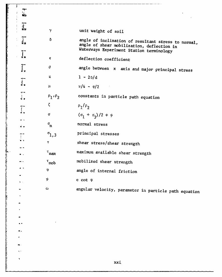
. 'V ? unit weight of soil
8 angle of inclination of resultant stress to normal,sli angle of shear mobilization, deflection inWaterways Experiment Station terminology
Rig deflection coefficient
e angle between x axis and major principal stress
I - 26/d
" p. r/4 - p/2
P constants in particle path equation
~pl/p 2
a(a I + a3) / 2 + pnormal stress
a 1,3 principal stresses
T shear stress/shear strength
-m maximum available shear strengthmax
T mob mobilized shear strength
(angle of internal friction
C cot q
0 angular velocity, parameter in particle path equation
xxi
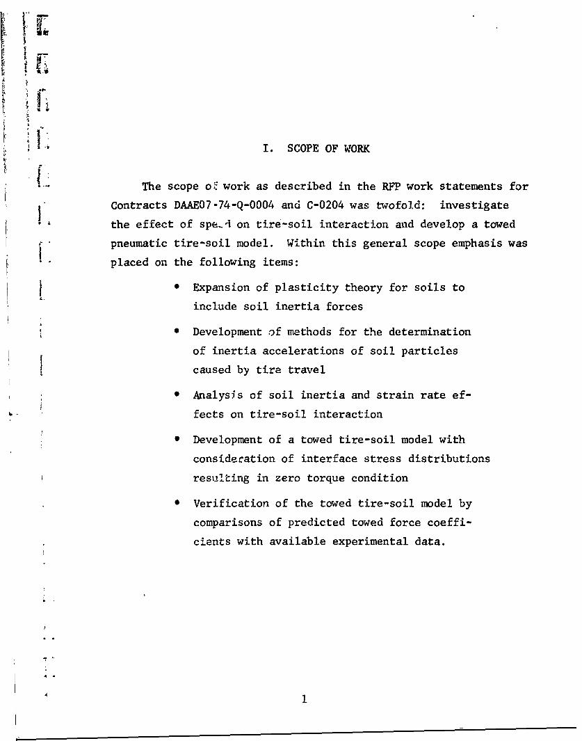
I. SCOPE OF WORK
The scope o2 work as described in the RFP work statements for
Contracts DAAE07-74-Q-0004 and C-0204 was twofold: investigate
the effect of spe-d on tire-soil interaction and develop a towed
pneumatic tire-soil model. Within this general scope emphasis was
placed on the following items:
Expansion of plasticity theory for soils to
include soil inertia forces
* Development of methods for the determination
of inertia accelerations of soil particles
caused by tire travel
Analysis of soil inertia and strain rate ef-
fects on tire-soil interaction
Development of a towed tire-soil model with
considecation of interface stress distributions
resulting in zero torque condition
Verification of the towed tire-soil model by
comparisons of predicted towed force coeffi-
cients with available experimental data.
m 1

II. EFFECT OF SPEED ON TIRE-SOIL INTERACTION
At present, tire-soil interaction theories are based on a
quasi-static model that assumes a steady state of the tire-soil
system. The tire is assumed to travel at a sufficiently low
jvelocity so that velocity effects are negligible. Yet experiments
performed under controlled conditions at WES (Ref. 1) show that
even in the low velocity range of off-road travel, velocity ef-
fects are far from negligible. In the higher velocity range of
aircraft landing gear-soil interaction velocity is one of the main
controlling factors that affects the drag load as experiments indi-
cate (Refs. 2 and 3).
Velocity affects tire-soil interaction primarily in the fol-
lowing two ways:
- Soil inertia forces are generated in the soil
during the passage of a tire. The magnitude of
these inertia forces depends on the velocity of
the tire and is approximately proportionate with
the square of the velocity of the tire.
* The strength of the soil that controls the inter-
face stresses is affected by the rate of loading
that is directly proportionate to the velocity
of travel.
Secondary effects of velocity on tire-soil interaction may in-
clude the increase of tire stiffness with an increase of the angu-
- - lar velocity of tire, the effects of velocity on interface friction
development, etc. No study of these effects was made in the pres-
ent research project.
Preceding page blank3I

III. EFFECT OF SOIL INERTIA FORCESON TIRE-SOIL INTERACTION
do
The concept of tire-soil interaction presented in Ref. 4 for
driven tires and Section VIII of this report for towed tires
assumes that the soil is in the plastic state of equilibrium, char-
+ acterized by slip line fields, whenever the normal stress corre-
sponding to this plastic state of stresses is less than the limit-
ing pressure characteristic of the tire. The geometry of the
zones of plastic equilibrium and the stress states in these zones
are defined by solutions of the differential equations of plas-
- ticity for soils. These differential equations are derived from
*the combination of the differential equations of static equilibrium
with the Mohr-Coulomb yield criterion.
The passage of a tire, even if it travels at a constant veloc-
ity, displaces soil particles within the affected soil mass. The
end result of soil particle displacement is the formation of a rut
behind the tire. Thus, during the passage of the tire a soil
particle moves from its original position at rest to a new one
where it comes to rest again. This particle motion involves ac-
celeration and deceleration of the particle and, as a consequence,
inertia forces are generated in the soil. To consider these inertia
forces in the differential equations of plasticity for soil, the
Mohr-Coulomb yield criterion has to be combined with the differen-
ti.al equations of motion instead of those of static equilibrium.
This combination, after the same manipulation of the equations is
performed as in the static case, yields the following differential
equations:
dz = dx tan(e F i)
- da:2a tan (de =Zi(a T (a +g)tan q)dx+(a +g± a tan 1)dzi5L Px za bldnk
5 Preceding page blank
In these equations x and z refer to a coordinate system
that moves with the tire, whereas a and a denote soil parti-x z
cle accelerations that refer to a fixed coordinate system. The
motion of soil particles as well as their accelerations are closely
related to the geometry of slip line fields. Since this latter
itself depends on the particle accelerations, as Eq. (1) indicates,
therefore, there is an interdependence between the accelerations
and other variables in Eq. (1). Even if a functional relationship
could be established among these variables, the direct numerical
solution of Eq. (1) would be a formidable task because of the in-
herent nonlinearities in these relationships. In an attempt to
develop a method that yields an acceptable approximate solution of
Eq. (1), two approaches have been followed and investigated in de-
tail. In the first, essentially theoretical approach the theory
of velocity fields associated with the slip line fields is applied
to the determination of particle accelerations. The second ap-
proach is based on an analytical simulation of observed particle
path geometries and is, therefore, a semi-empirical one. A de-
tailed discussion of these approaches together with an evaluation
of the numerical computational procedures developed for their ap-
plication to the tire-soil interaction problem is given in the fol-
lowing sections.
6

1
IV. DETERMINATION OF SOIL INERTIA FORCESBY THE THEORY OF VELOCITY FIELDS
Theoretical Background
Originally, the theory of velocity fields was developed in
connection with the application of the theory of plasticity to
metal forming processes. For metals the angle of internal fric-
v tion is zero and the characteristics obtained from the solutions
of the differential equations for both the velocities and the
stresses coincide. In the plastic state, frictionless materials
actually slip along the characteristic line; hence the term "slip
line field."
The theory of velocity fields was later extended for materials
exhibiting friction, such as soils. The purpose of this extension
was, however, not so much to determine the flow of the material,
as in the case of metal forming processes, but to enable research-
ers to apply the limit theorems of plasticity to various problems
of the plastic equilibrium in soils. The limit theorems of plas-
tic equilibrium state that a statically admissible stress field,
derived from the differential equations of the plasticity theory,
yields a lower bound for the collapse load, while collapse loads
computed for various kinematically admissible velocity fields
yield upper bound solutions. The true solution is when the lower
and upper bounds coincide.
The significance of the limit theorems of plasticity in engi-
neering applications is that the collapse load (or failure stresses)
may be higher than that computed from stress fields if the geometry
of the stress fields is kinematically inadmissible.
Derivation of the differential equations of velocity fields
is based on the assumption that the strain rate is proportional to
vi 7

I,the time rate of stress (Refs. 5 through 12). A system of partial
differential equations similar to that of the stress equations can I
then be derived. The solutions of this set of hyperbolic differen-
tial equations are the characteristics of the velocity field. Gen-
erally, the kinematic boundary conditions are insufficient to define
the velocity field and, therefore, the usual procedure is to ana-lyze the geometries of stress fields for kinematic admissibility.
If, however, for a frictional material the characteristics of the
velocity field are assumed to coincide with those of the stress
field, the strain rates associated with the velocity fields require
a rate of dilation of the soil that is unrealistic. Various theo-
ries have been proposed to deal with this problem but none of them
is completely satisfactory. It is outside the scope of this report
to discuss these controversial issues in detail; regarding the use
of velocity fields for the determination of soil inertia forces in
tire-soil interacticn problems the following considerations apply:
* If the stress boundary conditions are such that
they uniquely determine the stress field then
the problem is statically determinate, the char-
acteristics of the velocities coincide with those
of the stresses. The solution is the true solu-
tion since upper and lower bounds are identical
(Ref. 11).
* In tire-soil interaction problems boundary condi-
tions completely define the stress field, there-
fore, the solution is statically determinate and
it is the true solution. However, the assumption
of a uniform development of interface friction
along the contact area, although to some extent
supported by experiments, is an arbitrary one.
8

ID
Since interface friction depends on the kinematic
boundary conditions at the interface, the solution
of Eq. (1) is the true solution only, if the as-
sumed interface friction distribution is compati-
ble with the kinematic boundary conditions. The
establishment of the kinematic boundary conditions
at the interface is also necessary for the compu-
tation of velocities and is discussed in detail
under that heading.
Ii * In the following analyses it is assumed that the
characteristics of stress and velocity fields
coincide. Although this assumption is associated
with an unrealistic rate of dilation, in the case
of tire-soil interaction problems the velocity
field is an instantaneous one, and the dilation
prevails only for an infinitesimal time. Also,
the tire-soil models used for the calculation of
tire performance assume a steady state in soil
where the soil is already compacted by the tire
action to a significant degree. Therefore, the
soil is likely to dilate under the yield stresses.
In summary, flow fields in tire-soil interaction are main-
tained for an infinitesimal time, therefore, the rate of dilation
is not a critical consideration and the characteristics of stress
and velocity fields may be assumed to coincide. If the geometry
* of the characteristics is computed from the equations for the
stress field then the velocities can be computed from the follow-
ing equations (Ref. 10).
S. 9

dva + (va tan ( + vp sec ()de a 0 -
(2)dvB v sec (P + v tan (P) de =0
The above equations define the variation of velocities along
characteristic lines. The velocity vectors v and vp are com-
ponents (projections) of the velocity vector v in the direction Liof the "j" and "i" lines, respectively. It is noted that the
vectorial sum of v and v is not v (Fig. 1).
The v x and vz components of the velocity vector, v, are
related to v and v as follows
v =V sin e - v cos ex z
(3)v = v sin ep - v cos OP
x z
Since it is assumed that the velocity and stress characteris-
tics coincide, the angles ei and e. may be determined from the
stress field relation
ea
(4) :
For the numerical computation of the velocities the geometry
of the characteristic lines as well as the 0 values are computed
for the stress field and the velocities from the following differ-
ence equations: -
ta and are superscripts designating slip lines
10l.1

I
X
/ \ Line
I. \\ \ "
V "\-
* ± Line
I z
Fig. 1. Velocity Vectors Along Characteristic Lines.
/ B
Fig. 2. Boundaries of a Slip Line Field in
Tire-Soil Interaction Problems
11
av. (A- B C)/(1.O - B • D)
av' vij = C -D •vi~
where
a a
A Vi+l'J " Vi+lJ tan cP(ei,j -i+l,j)
I + tan '(e.. -e.
,3.' i+l,j(5)
B sec T(ei'j - ei+lj)T -TT+ t an (- ei' j - e i+l, j)
vi,j+I + 4vij+I sec p(ei j - ei,+l)
CI - Itanq(e. * -e ~+)
4 sec cp(ei, j -eij+)
D=1- tan P(e - e )IJ i~j+1)
The difference equations (5) indicate that for given stressfield characteristics the velocity for a grid point i,j can be
computed if the velocities at two adjacent points (i+l,j and
i,j+l) are known. The kinematic boundary conditions, discussed
under the next heading, provide the initial values of velocities
necessary to start the numerical computations.
Kinematic Boundary Conditions
In a slip line field determined by the differential equations
of plasticity for soils by methods discussed in detail in Refs. 13
through 18 there are three boundaries where kinematic boundary con-
ditions are to be examined (Fig. 2). At the stress free surface
AB it is assumed that there are no kinematic constraints and
12

points at the surface may be displaced freely. The boundary BCDE
is the outermost slip line beyond which the soil is not in the
state of failure. Implicit in the use of the Mohr-Coulomb yield
criterion is that soil deformations prior to yield are disregarded,
therefore, in this concept the soil beyond the outermost slip line
- acts as a rigid body. Consequently, velocities across this bound-
ary must be zero, resulting in the kinematic boundary condition
- vB = 0 for this line. For this boundary condition Eq. (.) is
integrable and yields
a aL ~a =~a * tan1 p(e -e0(6•"v =v 0 e (6)
I Note that for the stress computations the state of the soil
outside the slip line field is immaterial. The velocity field,
i hhowever, is profoundly affected by the assumption that the soil
I .adjacent to the outermost slip line is assumed to be rigid. Ex-
perimental information on soil displacementq along this boundary
is scarce. It appears that while the soil mass outside this
boundary undoubtedly undergoes some deformation there is an abrupt
change in the displacements in a narrow band along the boundary.
Thus, the theoretical boundary condition corresponding to the
rigid-plastic material idealization may not be too far off from
reality.
As stated before, the critical kinematic boundary conditions
are those at the tire-soil interface. The distribution of interface
friction along this boundary must be consistent with the kinematic
conditions there if the slip line field solution is to be the true
solution for the yield stresses. As a result of detailed studies
of the kinematic conditions at the interface, new concepts of slip
j oand interface friction were developed. These are not only useful
for the definition of boundary conditions for velocity fields but
13

also offer new insight in the not very well understood area of
slip-interface friction relationships. The results of these kine-L
matic analyses and the reasoning that led to the development of
these new conce-ts regarding interface friction are presented in
the following discussions.
The kinematics of a point attached to the surface of the tire L
are easily determined if the geometry of the tire centerline and
the angular and translational velocities of the tire are known.
The trajectory of such a point, in a fixed coordinate system is
shown in Fig. 3 for a complete revolution of a slipping tire. The
L.
Fig. 3. Trajectory of a Point at theCircumference of a Deformable Tire
point describes a prolate cycloid when its position is in the un-
deflected part of the tire; otherwise the trajectory is an irregu-
lar curve corresponding to the assumed tire deflection. The hori-
zontal and vertical components of the velocity of the point may
also be easily determined since both the angular and translational
velocities are assumed to be constants.
For the determination of the velocity boundary conditions
that apply to the slip line field in the soil the velocities im-
parted to a soil particle at the interface are needed. These are
related to the velocities of a point attached to the tire surface
14

a' but are by no means identical. A fundamental aspect of the analy-
sis of the kinematic conditions at the interface is that the inter-
L face must be considered as consisting of two faces: one being the
- surface of the tire, the other that of the soil. It is assumed
that these two faces of the interface may slide on, but may not
separate from each other. This latter assumption leads to the
I . condition that the normal components of the velocities of the two
,- faces be the same at every point. This condition, however, is by
S.it itself insufficient for the determination of soil particle veloci-
-- ties at the interface. The additional assumption is made that the
direction of the velocity vector of a soil particle coincides with
the direction of the major principal stress in the slip line field.
For homogeneous isotropic soils with linear stress-strain relations
*this assumption follows from the theorems of continuum mechanics;
I.f for soils not meeting the above criteria strictly the assumption
is only approximately valid. With these assumptions the velocities
of soil particles at the interface (that constitute the velocity
boundary conditions) can be determined as follows.
The velocity vector for a point at the tire surface may be de-
termined by vectorially adding the forward velocity vector (vf)
and the tangential velocity vector (vt) (Fig. 4a). The tangen-
tial velocity vector is the component of vector vp (peripheral
velocity) in the direction of the deflected surface of the tire
v =r =vf/(l s)
(7)
- v cos(a -a')p
The horizontal and vertical components of the resultant veloc-
ity vector are
15

xzf
) a
1
V.n b)
z
Fig. 4.Kinematic Boundary Conditions at the Tire-Soil Interface.a) For the Tire b) For Soill
16

SV x =vf -v cos(a - a')cos a'
v =v cos(a - a')sin a' (8)z p
v v sin a' + v cos a' =v sin a'zn X f
This last equation expresses the fact that the component of
the velocity vector normal to the deflected surface of the tire
depends only on the forward velocity and is independent of slip.
For a soil particle at the interface the normal component of
the velocity vector can be computed as (Fig. 4b)
tS S * S Iv= v sin a + v cosa =vf sin a'V.n x z
(9)• --- = tan e'
SvZ
From Eq. (8) the horizontal and vertical components of the
velocity vector can be expressed as
s sin a'Vx f sin a' + cotan 0' cosa'
(10)is sS-v = v cotan e'
z x
- The velocity vector of a soil particle at the interface can
also be thought of as being composed of the forward velocity vector
* - and a tangential velocity vector. This latter can be computed from
the fo7i;:ui.ng equation:
-. - v t V ... r(ivf -a' tan e' + cos a'
tSuperscript s designates soil particle velocities
.. * 17

The tangential velocity computed by Eq. (11) for a soil parti-
cle is in the case of driven tires generally less than the tangen-
tial velocity computed by Eq. (7) for a point at the surface of
the tire indicating that a relative displacement occurs between
the soil and the tire. From the value of the tangential velocity
of a soil particle a hypothetical slip value may be computed as
s= I - cos(a - a') • (sin a' tan e' + cos a') (12)
It is interesting to note that this hypothetical slip value
is independent of the translational velocity of the tire, at least
for the assumed steady state concept of tire-soil interaction.
At this point it is worthwhile to consider the meaning of the
hypothetical slip value determined by Eq. (12). If the tire ac-
tually turned with an angular velocity that resulted in a slip
equal to s' then there would be no differential displacement be-
tween the surface of the tire and the soil. Therefore, the hypo-
thetical slip sI may be termed as "contact slip." On the other
hand, the difference between s and s' is the result of dif-
ferential displacement between tire surface and soil. The term
"spin" conveys the idea of a tire rotating relative to a nonyield-
ing surface and is also expressive of the relative motion between
a tire and a yielding surface, therefore it will be used herein to
designate the quantity s - s'.
To further elucidate the meaning and significance of these
terms a track element may be considered (Fig. 5a). If a track ele-
ment displaces the soil by AL but stays in contact with the soil
while the vehicle travels a distance L then the "contact slip" is
s, L - AL. AL (13)
18

v-
* U', a )A~L
AX AL
b)
Fig. 5. Contact Slip (a) and Total
Slip (b) of a Track Element
However, if the track element slides over the soil and at the
end of vehicle travel L is displaced by AX relative to its
original position (Fig. 5b) then the total slip is
AX + ALL (14)L
In the case of a track element it is easy to visualize the
meaning of the two slip values s and s'. In the case of tire-
soil interaction the assumption of a steady state in the soil
leads to the concept that the slip line fields move with the tire
I:while the soil particles are displaced from their original positionwith respect to a coordinate system that is fixed to the ground.
This concept makes it somewhat difficult to visualize the relative
-- 19
displacement of the tire surface to the soil. However, the meaning
of the terms introduced by Eq. (12) is essentially the same as ex-
plained for a track element.
In the foregoing discussions velocities of a point at the sur-
face of tire and soil were defined and compared. On the other hand,
the conventional definition of slip relates slip to actual and
theoretical distances traveled by the tire. Obviously, the con-
ventional slip value determines an overall slip for the tire.
Janosi (Ref. 19) and others have pointed out that the slip for an
infinitesimal element of a rigid wheel may vary along the interface.
In the case of pneumatic tires infinitesimal elements of the sur-
face of both tire and soil may deform and exhibit different dis-
placements relative to each other. As a result, a variation of
slip along the interface may easily develop.
The kinematic boundary conditions and Eq. (12) derived from
these conditions allow the computation of contact slip for every
point at the interface once the tire centerline geometry and the
associated slip line fields have been determined. For the determi-
nation of the slip line fields in the tire-soil model the angle of
interface friction is assumed, or computed from the modified
Janosi-Hanamoto equation
tan 6 =tan 6 (1 e(S+S0) (15)
for given slip and slip-shear parameters. Equation (15) refers to
the conventional value of slip. In the model, slip and interface
friction angle are 'assumed to be constant along the interface.
For these conditions the variation of the contact slip along the
interface in the tire-soil model was determined for several loading
conditions, tire types, and conventional slip values. It was found
20

lw that the variation of the contact slip along the interface was
- minimal and its value less than the conventional value of slip.
Typical variations of the contact slip along the interface
are shown in Fig. 6 as a function of the central angle. The con-
tact slip values were found to vary little along the interface in
the cases investigated. Largest deviations from the average value
were found near the exit angle where the tire centerline geometry
1' shows an upward curvature. Kinematically this portion of the
interface is the most problematic since the kinematic boundary
V- conditions as set forth in the foregoing paragraphs require that
the velocity of the soil particle be upward directed so that no
" separation of soil and tire surface occurs.
The concept of contact slip has important implications for
both the theory of tire-soil interaction and the practical aspects
of off-road vehicle engineering. The contact slip represents the
absolute minimum of slip at which a certain tire performance can
be realized. In the tire-soil model the tire centerline geometry
as well as the directions of the principal stresses along the in-
terface are computed and from this information contact slip values
for every nodal point at the interface can be determined. Since
the variation for the contact slip values along the interface is
minimal, an average value of the contact slip may be computed and
relationships between the development of interface friction angle
and the average value of the contact slip may be established for
various conditions. Thus a theoretical basis exists for analysis
of the relationship between interface friction angle and contact
slip. This relationship may be compared with Eq. (15) that repre-
sents the relation with the conventional slip value.
The concept of contact slip and the method of analysis that
allows its determination for various soil and loading conditions
21

K
J
O;
0.15
-x-.'- Contact Slip
0.10 ....... Average of -Contact Slip /
0.05/
-10 0 10 20 30 4o
Central Angle a
Fig. 6. Variation of Contact Slip Along the Interfaceof a 9.00-14 Tire in Yuma Sand. Load 620 Ibs;Conventional Slip: 15%; Cone Index Gradient:15 lbs/cu in.
22

4
opens new avenues of research that could lead to economics in off-
road vehicle engineering. Obviously, spin, the differential dis-placement between tire and soil surface, is undesirable since it
is the primary cause of tire wear and results in a waste of energy.
For understanding of the phenomena that causes spin a systematic
analysis of the contact slip and its relation to the conventional
slip, soil, and loading conditions.preferably coupled with ex-
perimintal investigations, would be needed. These would include
measurements of soil particle displacements at the surface as well
as torque rather than slip-controlled performance tests.
- Computation of Inertial Accelerations from Velocity Fields
The concept of tire-soil interaction for which the mathemati-
cal model was developed (Ref. 13) assumes that steady state condi-tions exist in the soil. This assumption is equivalent to stating
that the slip line fields travel with the tire with the same
velocity. For these conditions the computation of accelerations
becomes very simple if the velocity fields are known. In an in-
finitesimal At time increment the velocity of a soil particle at
any point x,z changes to the velocity at x - Ax,z where
, x = vfAt. The velocity field computation yields the velocity com-
ponents for every nodal point in the slip line field. The numeri-
cal computation of the a~czelerations for these nodal points re-
quires the determination of the velocities for a Ax change. This
is accomplished by assuming a linear velocity change between the
nodal point in question and two adjacent nodal points, one along
the "i" and one along the "j" line. At the boundaries of the
slip line field, velocities at these points are not always avail-
able and other combinations of adjacent nodal points had to be
selected for the determination of accelerations.
23

Computational Scheme for the Consideration cfSoil Inertia Forces in Tire-Soil Interaction L
For analysis of the effect of soil inertia forces, computed
on the basis of velocity fields, a computer program was prepared. I_This computer program computes the interface stresses for a given
entry, rear and separation angles for various translational veloc- Iiities of the tire. The soil inertia forces considered in the
program correspond to a constant translational velocity of the
tire.
The program represents a numerical solution method for the -i
differential equations (1). It computes the soil inertia forces
by successive iteration. In this iteration the first step is to
determine the slip line 'field geometry without soil inertia forces,
i.e., for vf = 0. Then on the basis of this slip line field
geometry the velocity fields and accelerations are determined for
each nodal point for a selected velocity increment. It is assumed
that the accelerations computed for each nodal point are valid
when a new slip line field geometry is computed on the basis of
these accelerations. This iteration scheme in the computer pro-
gram is included in an interactive manner that allows study of the
effect of the selection of velocity increments as well as the
effect of repeated iterative acceleration computations on the slip
line field geometry. A detailed flow chart for the program is
given in Appendix A.
Problems Encountered with Development ofthe Computer Program
Numerous minor problems were encountered with development of
the program because initially the same iteration and interpolation
schemes were used in the program as in the case without inertia
24

forces. The consideration of inertia forces in Eq. (1) resulted
-- in a more complex situation where the behavior of soil was often
Isl different from that anticipated on the basis of previous experi-
-- ence and, therefore, iteration and interpolation schemes had to be
modified. Other problems that have broader significance are dis-
cussed below.
The starting point for the development of this computer pro-
gram was the one prepared for the simulation of tire-soil interac-
tion presented in Ref. 13. In that program an ixj = 48 x 16
grid is set up for the computation of a slip line field, but only
as many j lines are computed as are necessary to end up with the
boundary j line at a prescribed location at the interface. The
boundary j line is obtained by interpolation between evenly
spaced j lines. This technique was developed to reduce the com-
puter time that would be necessary to find the required size of
the slip line field for a preset number of j lines.
Initial application of the same technique to the present prob-
lot 1 m created difficulties, because the number of j lines may
-. c1ahge in the various slip line fields when inertia forces are
taken into account. In the iteration technique where the slip
. line field geometry is updated for velocity increments a variable
number of j lines is undesirable,because for an updated slip
- -line field geometry containing more j lines than the previous
field, accelerations for points on the additional j line are not
available. For this reason the technique using a variable number
of j lines was discontinued in this program and a constant
- 30 x 10 grid size was adapted. It was found that although the
- computer time needed to perform the necessary iterations to find
- the required size of the slip line field increased considerably
for the first slip line field, in the subsequent iterative proce-
dure for the updating of the slip line field geometries the
25
changes in the size of these fields were small and the total com-
puter time was comparable to that needed with variable j lines.
The boundary conditions for the stress field also presented
problems when inertia forces were included. The soil surface out- I__side the tire-soil contact area was initially assumed as stress
free and the direction of the major principal stress as horizontal
even if soil inertia forces were included. Examination of the
geometries of slip line fields generated with this assumption
clearly showed an abrupt change in the directions of slip lines
at the first row of nodal points beneath the free surface. In
further analyses the direction of the major principal stress at
the surface was assumed to correspond to a hypothetical loading in
the direction of the resultant inertial force. Slip line fields
generated with this assumption were smooth and this assumption was
adapted in the further development.
The singular point (Point "A" in Fig. 2) presents special
problems when inertial accelerations are included in the computa-
tions. Stresses at this point are computed by the equation
2 tan c(e-e )= 0 e (16)
that is the solution of differential equations (1) when both dx
and dz vanish. It is seen that the inclusion of inertial accel-
erations does not affect the validity of Eq. (16) since all in-
ertial terms are multiplied by the vanishing dx or dz differ-
ential. The singular point can be regarded as a degenerate jline (with zero length) alnng which e changes from its value e
at the adjacent free surface to that specified at the adjacent
interface. However, for the determination of e the inertial0
accelerations would have to be known at the singular point con-
sidered as part of the free surface. For the computation of these
26

acceleration velocities at this point, themselves dependent on eo,
would have to be computed. Since the neighborhood of the singular
point and the singular point itself is a critical part of the solu-
tion for the whole slip line field, it was necessary to develop
and adopt an updating procedure for the computation of e0 and0
velocities for this point independently of the updating of the
rest of the field. The problem of updating the solution of the
differential equations in the neighborhood of the singular point
was compounded by the difficulties of applying the numerical tech-
S- niques to the solution. The assumption of a linear variation of
I •velocities from an i,j point to an i,j+l and i+l,j point
- -(applied for acceleration computations at an inner i,j point of
1. the velocity field) is clearly inapplicable to the singular point
- that is the common location of nodal points with various i desig-
nations. The assumption of linearity would lead in this case to
either infinite, or undetermined accelerations. Thus, it was
I 'necessary to compute the theoretical accelerations at the singular
point from another combination of points along the next j line.
*+ An extensive analysis of the acceleration computation was made
using various grid sizes and combinations of two or more points
* along the j+l line. From these analyses it was concluded that
*while different numerical techniques affected the value of accel-
eration computed for this point the problem is a physical one:
: - with increasing translational velocity the location where acceler-
ations become critical first is that of the singular point. This
could be expected since the singular point is also the entry point
where the tire "hits" the ground. Accelerations at the singular- +point are critical when the inclination of the major principal
S " stress associated with these accelerations equals that at which
the free surface becomes a slip line. There is no single valued
solution for the slip line field when the accelerations at this
" point exceed this limit.
27

I
The geometries of updated slip line fields generated with the
4 iterative procedure for the computation of inertial accelerations
were transmitted to a plotting program subroutine that allowed the
vicual examination of the updated geometries. This examination
revealed that in many cases when the numerical end results appeared
to be acceptable the numerical solution of the differential equa-
tions (1) was multivalued, as evidenced by the overlapping of the
slip .lines. A slip line field with an appreciable overlap is
shown in Fig. 7. In many cases the overlap was hardly noticeable
Fig. 7. Overlap of Slip Lines in the Case of a Multivalued Solutionof the Governing Differential Equations
upon visual examination of the slip line field, therefore, a pro-
vision was made in the program to indicate by a printout if, within
the accuracy of calculations, overlap occurs. Overlap indicates
that the mathematical solution of the differential equations (1)
at a particular location is multivalued, i.e., more than one a
and e value belongs to the same x,z point in the slip line
field.
The importance of an overlap indicating multivaluedness of
the mathematical solution is that the solution no longer represents
the physical behavior of soil under the applied loads, since it is
a physical impossibility to have two different stress states in the
soil at the same place and at the same time. Thus, overlap is a
limitation to the application of plasticity theory with inertial
28

Qw forces to the tire-soil interaction problem. Since with the method
of velocity fields, overlapping starts to occur at relatively low
velocities (in the range of 5 feet/second); this limitation is a
serious one. Therefore, an extensive investigation was made to
determine the causes of the overlap and especially, whether the
overlap is the result of the application of numerical techniques
or is inherent in the problem. As a result of these investigations
the following conclusions were drawn:
v 1. Overlap occurs if there is 4'n abrupt change in
Ithe magnitude of inertia forces between adjacent
nodal points. The geometry of the slip line
fields is such that while there are no abruptchanges in the velocities along the slip lines,
there are abrupt changes in the derivatives of
the velocities at locations where the various
zones (active, passive, and radial) are joined
together. This is evident in the case of
Prandtl fields for weightless soil where straightV slip lines are joined with logarithmic spirals
at the zone boundaries. Numerical computation
techniques can aggravate this problem if at the
zone boundaries a different set of nodal points
°" is used for the acceleration computation than
inside the field. Numerical computation tech-
niques can alleviate the problem by using schemes
that tend to smooth these abrupt changes.
2. Overlap usually occurs first in the neighborhood
of the singular point. Bow waves change the
geometry of free surface in a way that the ef-
fect of inertia forces in the neighborhood of
the singular point is counterbalanced.
29

3. The velocities determined by the theory of
velocity fields are based on a two dimensional
model of the tire-soil interaction. Implicit
in the model is that soil particles may move
only in the plane of travel. In actuality the
movement of soil particles is not restricted
to the plane of travel and, as a consequence,
the actual velocities and accelerations are
less than predicted by the two dimensional
theory.
Results of Sample Computations
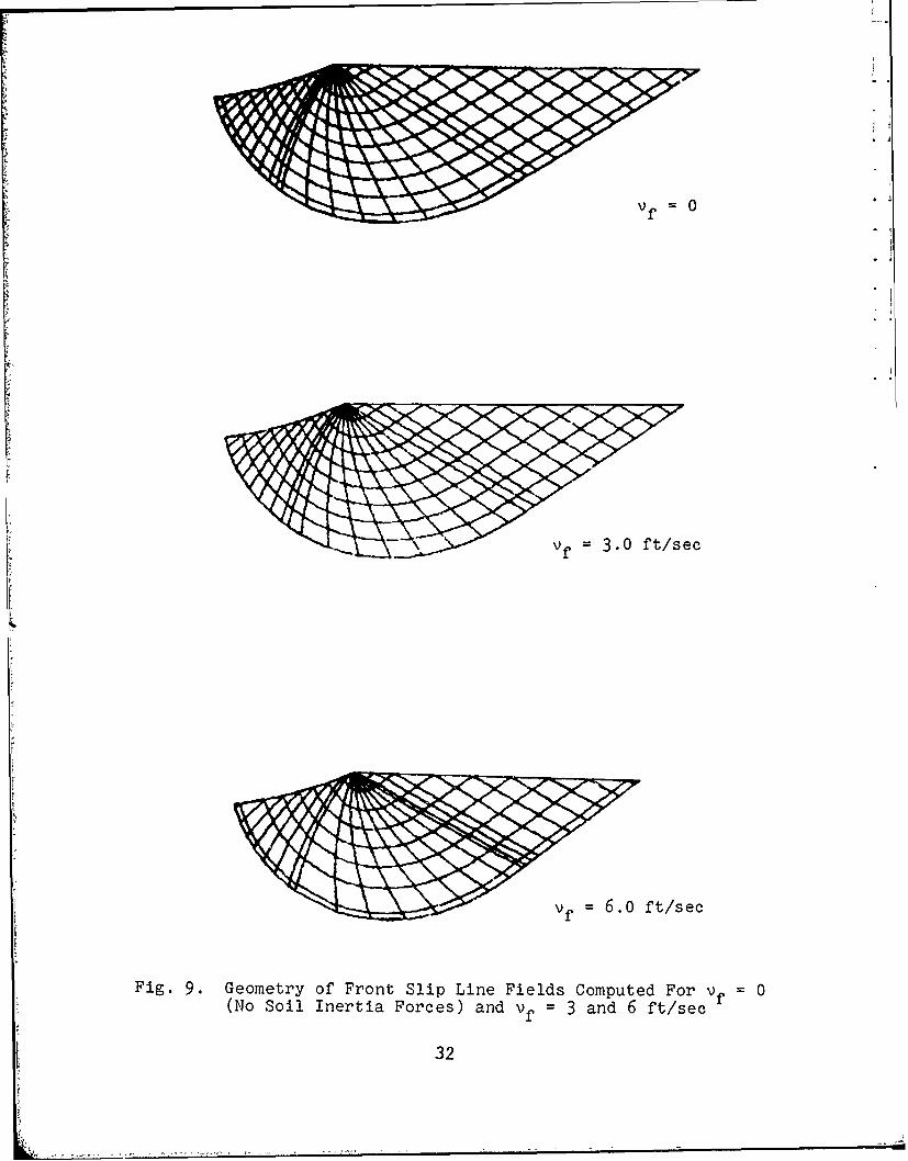
For the evaluation of the effect of inertia forces on tire
performance sample computations were made within the velocity
limits imposed by the criterion that the solution should be single
valued. The results of these sample computations were surprising
in that the effect of inertia forces was minimal even though the
computed inertial accelerations often exceeded g by a factor of
10 or more. Figure 8 shows a comparison of normal stresses com-
puted with and without inertia forces generated at a translational
velocity of 5 feet/second. There is a slight, almost impercepti-
ble rise in the normal stresses in the front and a very slight
decrease of them in the rear of the tire when inertia forces are
accounted for. Table I shows the pertinent input and performance
data.
Figure 9 shows the geometries of front slip line fields de-
termined for 0, 3, and 6 feet/second translational velocities,
respectively. Although changes in the geometry with the velocity
appear to be minor, closer observations of the "i" lines shows
their approaching each other in the vicinity of the boundary be-
tween the passive and radial zone, an indication of an impending
overlap situation.
30

1000
L800
.-.
02600
00
V 2
!" " 00 ,X Vf =l5 ft/sec2I00
o, =
0 -10° 0 10 20 30 400
Central Angle a
Fig. 8. Normal Stress Distribution With/Without Soil Inertia Forcesfor Tire Loading and Soil Conditions Shown in Table 1.
Summary Discussion of the Method of-* Velocity Fields and Conclusions
A computer program has been developed that takes soil inertiaforces in tire-soil interaction into account by computing the
velocity fields associated with the slip line fields and the ac-celerations therefrom. It was found that the method can be usedup to about 5 feet/second velocity with 9.00-14 tires (for
larger tires probably up to proportionately higher velocities)
31
vf 0
f. = 3.0 ft/sec
Vf 6.00ft/sec
Fig. 9. Geometry of Front Slip Line Fields Computed For vf = 0(No Soil Inertia Forces) and vf = 3 and 6 ft/sec
32

TABLE I TIRE PERFORMANCE WITH AND WITHOUTSOIL INERTIA FORCES
(Method of Velocity Fields)
Tire Size: 9.00-14
Tire Radius (nominal): 1.18 ft
I Tire Width: 0.70 ft
Inflation Pressure (pi): 12.5 psi
L Slip: 15%
Angle of InterfaceFriction: 15.7 °
Front Field Rear Field
Cohesion 15 lbs/sq ft 30 lbs/sq ft
i Friction Angle 240 280
Unit Weight 100 lbs/cu ft 105 lbs/cu ft
Translational Velocity vf = 0 ft/sec vf = 5 ft/sec
Load 408 lbs 410 lbs
Drawbar Pull 48 lbs 53 lbs
Torque 129 ft-lb 135 ft-lb
Sinkage 2.03 in. 1.81 in.
Pull Coefficient 0.119 0.129
when the solution of the differential equations becomes multivalued.
Because of the two dimensionality of the velocity fields, veloci-
ties and associated inertial accelerations are overestimated by
this method. It was found that abrupt changes in inertia forces
occur inherently in this method because derivatives of slip line
directions that control the velocity field are discontinuous at
the joint boundaries of the active, passive, and radial zones.
33

There is no experimental information on the physical phenome-
non that occurs when the plasticity solution becomes multivalued.
Speculatively, one may assume that failure in the classical Coulomb
sense cannot occur and a so-called "rigid" soil zone exists within
the bounds of overlap. It is also likely that the soil adjusts
itself and seeks to fail along slip lines with continuous curva-
ture. Upper bound solutions based on the characteristics of the
differential equations for velocities would have to be considered
rather than solutions based on stress characteristics. A possible
solution would be a slip line field with only one zone and con-
tinuous curvature of the slip lines.
Inertia forces appear to have little effect on tire perfor-
mance as long as the plasticity solution is single valued. A
slight rise in the normal stresses in the front field increases
tire deflection thus resulting in a slightly better tractive per-
formance. It should be noted that even though the calculations
were made for a low translational velocity the calculated inertia
forces inside the field were in the range of several, often more
than 10 g-s.
An incidental but important result with this method is the
introduction of a new concept, that of "contact slip" in the tire
soil interaction problem. For determination of the contact slip
in any interaction problem, only a small portion of the computer
program, dealing with the kinematic boundary conditions, is needed.
The new concept can be the basis of further theoretical research
in the area of slip, mobilized shear, and traction development.
34

U.' V. DETERMINATION OF SOIL INERTIA FORCESBY THE PARTICLE PATH METHOD
Introduction
Soil inertia forces are generated by the acceleration and
deceleration of soil particles during the passage of a tire. The
motion of soil particles follows a particle path that defines the
geometry of particle motion in a coordinate system fixed to the
ground. Velocities and accelerations are time derivatives of the
coordinate vectors of particle path.
Experimental Information on Particle Path Geometry
Measurements of particle paths beneath rigid wheels were per-
formed by several researchers under laboratory conditions (Refs. 20
through 22) using the flash X-ray technique. These experiments
show the same general pattern and dependence of the particle path
on slip, as shown, for example, in Fig. 10. Although not pointed
out in the referenced publications that describe these particle
-path measurements, theoretical considerations indicate that for a
constant velocity the particle path geometry must not change with
-othe x coordinate, the direction of travel. Any variation in
particle path geometry in the x direction obtained in experiments
* must be the result of experimental error, inhomogeneities in the
soil bed preparation, etc. The invariability of the particle path
geometry with respect to the direction of travel also follows from
the "steady state" concept of tire-soil interaction.
The experiments show, on the other hand, that the size of
particle paths diminishes with the depth beneath the wheel and
there is a certain limit depth below which the soil is unaffected
by the passage of the wheel.
35

+
0
18.5% Slip Rate0o0.4 /
Particle Motion at .- -
1.2 Inch Depth 4 0.2 J.
i "°° --- S
II - I°" -
-0.4 -0.2 0 " " 0.4 0.6. I
Horizontal Motion--+ Ins. 5s% " | I a
S , -0.2 -\ ' DI ;l
3 S RatI /48.4/ Si /
(From Ref. 21) ,
"-0.6 23%SipRt
432.3% Slip Rate
Fig. 10. Particle Motion as Influenced by Slip Rate
(From Ref. 21)
There are some conditions that define the end points of the
path of particles that were originally at the surface. After the
passage of the tire these particles wind up in the rut at some
depth, that evidently equals the vertical distance between the end
points of the path. Experiments also show that the horizontal posi-
tion of a particle at the surface is changed by the action of the
wheel as it passes over the particle. In the case of a slipping
36
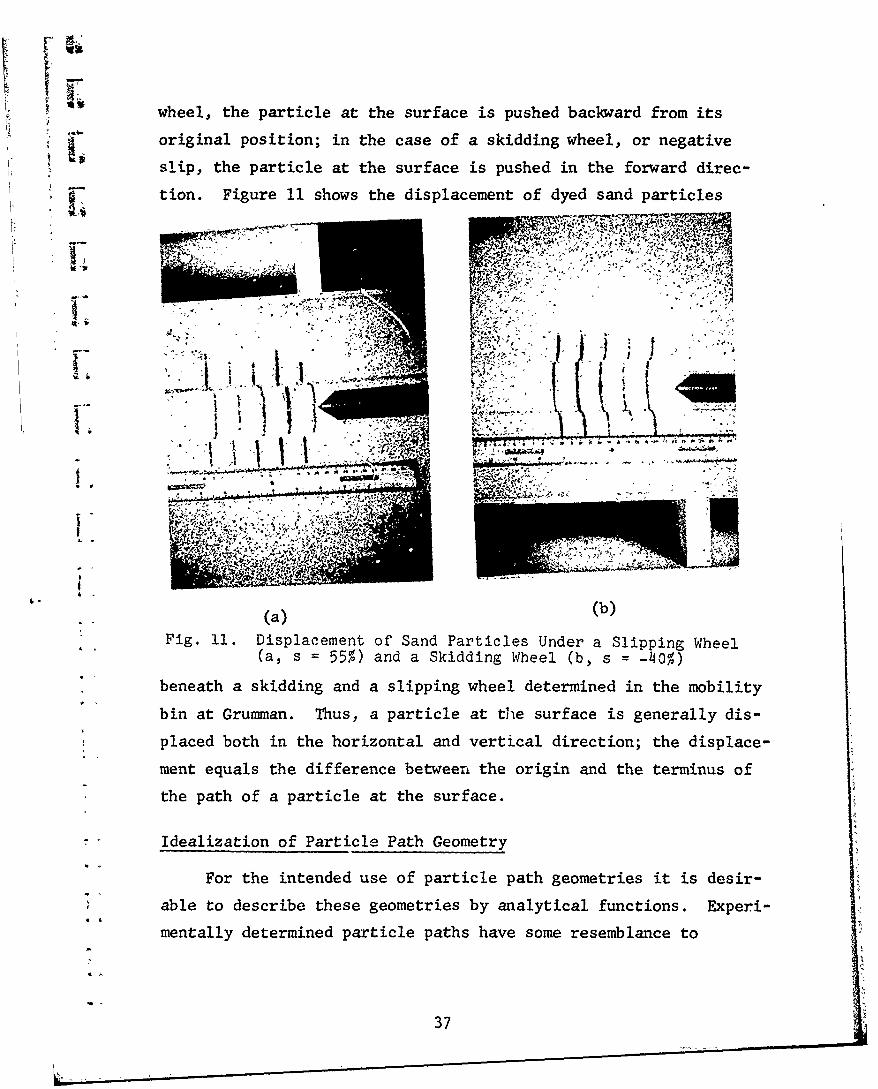
wheel, the particle at the surface is pushed backward from its
original position; in the case of a skidding wheel, or negative
slip, the particle at the surface is pushed in the forward direc-
tion. Figure 11 shows the displacement of dyed sand particles
(a) (b)
SFig. 11. Displacement of Sand Particles Under a Slipping Wheel(a, s = 55%) and a Skidding Wheel (b, s = -40%)
beneath a skidding and a slipping wheel determined in the mobility
$ bin at Grumman. Thus, a particle at the surface is generally dis-
~placed both in the horizontal and vertical direction; the displace-
ment equals the difference between the origin and the terminus of
the path of a particle at the surface.
SIdealization of Particle Path Geometry
For the intended use of particle path geometries it is desir-
" able to describe these geometries by analytical functions. Experi-mentally determined particle paths have some resemblance to
37 J

cardioids and in some publications they are referred to as such.The parametric equation of a cardioid is (Fig. 12)
x = 2a sin w - a sin 2w
z = 2a cos w - a cos 2w (17)
I A
Fig. 12 Cardioid Geometry
Obviously, a cardioid is not a suitable curve to describe theparcicle path when constraints are set for the displacement of theend point in both the horizontal and vertical direction.
Another curve that has a shape similar to the observed parti-cle paths is the nephroid. The parametric equation is (Fig. 13)
x = 3a sin w - a sin 3w
z = 3 a cos w - a cos3w (18)
38

4 i-
Fig. 13 Nephroid Geometry
A study of the shape of these curves showed that even if the
constraints for the end conditions could be met by selecting only
a portion of these curves for particle path simulation, more free-
dom is needed to describe particle paths under the wide variety of
soil and tire loading conditions. Also, the experimental informa-
tion is restricted to the case of rigid wheels and it can be
assumed that the simulation of the effect of tire deflection on
particle path geometry would require more freedom in the analytical
expression. This freedom is achieved by allowing the constants in
the above expressions to vafy as
x = a[p, sin w - sin plw]
(19)
z = a[P2 -1 P2 cos w + cos p2w]
39

Equation (19) refers to a coordinate system with its origin
coinciding with the initial at rest position of the particle. The
expansion of the expression in parentheses for z by the term
(P2 1) serves this purpose.
Equation (19) contains parametric exnressions of the particle
path that represents a family of curves of various shapes. Fig-
ure 14 shows variations of the geometry as defined by Eq. (19) for
various values of the parameters p1 and p2 . Equation (19) also
represents the geometry of the particle path in parametric form.
Time derivatives of the coordinates x and z yield the veloci-
ties and accelerations of the particle at the time the particle is
at point x,z. To calculate these time derivatives the parameter
w has to be related to time, t, preferably by a differentiable
function. If
= f(t) (20)
then the time derivatives of the coordinates of the particle path
are
x = aP!(Cos W - cos pl0)
z = w - sin p2w)
. 2 (21)apl (COS w - cos pw ) + apl(w)2(-sin w + p1 sin p1 w)
z =aP2w(sin w - sin p2 w) + aP2(w)2(cos w - P2 cos p2w)
To compute the accelerations from Eq. (21) the relationship
between the parameter w and time, t, has to be defined. To
this end it is useful to consider the changes in the direction of
the particle movement that can be associated with the relative po-
sition of the tire. The direction of the particle at any point
40

P1 2.9 P2 2.9 29P 8xP
p 1 =2.9 p 2 *9.p P1 p = . .. p
Fig. 114. Particle Path Simulation by Eqs (19)
41

along the particle path is given by the tangent of the path at
that point. From Eq. (19) the tangent of the particle path can be
calculated as
- dzdz dz P2 sin w - sin POdz K -- P2 - (22)dx dx Pl cos W -cos p(2
dw
The points along the particle path that may be associated with
various positions of the tire are shown in Fig. 15. The value of
the parameter at these points may be determined from the condition
that the tangent of the particle path is either horizontal or ver-
tical. The fcllowing tabulation shows the w values at these
points.
TABLE 2 VALUES OF THE PARAMETER wAT VARIOUS POINTS OF PARTICLE PATH
Point Tangent
A Vertical 0
B Horizontal v/(l + p2 )
C Vertical 27T/(1 + pl )
D Horizontal 3w/(l + p2 )
E Vertical 27r/(P 2 - 1)
The position of the tire that may be associated with the
above points and the time elapsed while the tire passes from one
point to another is shown in the lower part of Fig. 15. Obviously,
there is no rigorous time relation between these particle locations
and tire travel positions and these considerations serve primarily
as a guide for the mathematical formulation of the w = f(t) re-
lationship.
42

B
C
E
V D
f
1*1 viAt~BA
Point of Patil Pat
Fi .1 . R l t o et e n P s t o f T re a d C a a t r s iPoins ofParicleP4t

As mentioned before, for a particle at the surface the end
points also have to meet certain conditions. First, the vertical
distance between the end points must equal the rut depth, i.e.,
zE zA z r (23)
The constant "a" in Eq. (19) is selected so that this condition
be met.
Second, the assumption is made that the horizontal distance
between the end points equals the contact slip times the rut depth,
or
xE -x A- - s (24)zE - A
If in Eq. (19) the x,z values are substituted with the
values given by Eqs. (23) and (24) and with the appropriate value
oE the w parameter given in Table 2 then a relationship between
p1 and s' can be obtained. This relationship is shown in Fig-
ure 16 for P2 values varying from 0.75 p1 to 0.95 p1. It is
seen that within these limits the value of p1 is affected but
little by the value of P2, and Fig. 16 could be used for the es-
timation of p1 for any value of the contact slip s'. On the
basis of the available experimental information on particle paths,
it appears that a P2 value of about 0.9 p1 is a reasonable
assumption. Should further information on particle paths become
available, any other value of P2 that allows a good simulation
of particle path may be selected. In this case the value of p1
may be computed from the following polynomial determined as best
fitting the curves shown in Fig. 16.
44

Li-
14
I CI)
1 4 -3
-
0
o 2 =0.95 x Pl
P2 0.75 Pl '
2.5 3.0 4.o 5.0Pl
II
Fig. 16. Relationship Between Pl and s" for P2 Varying Between0.75 Pl and 0.95 Pl1
45
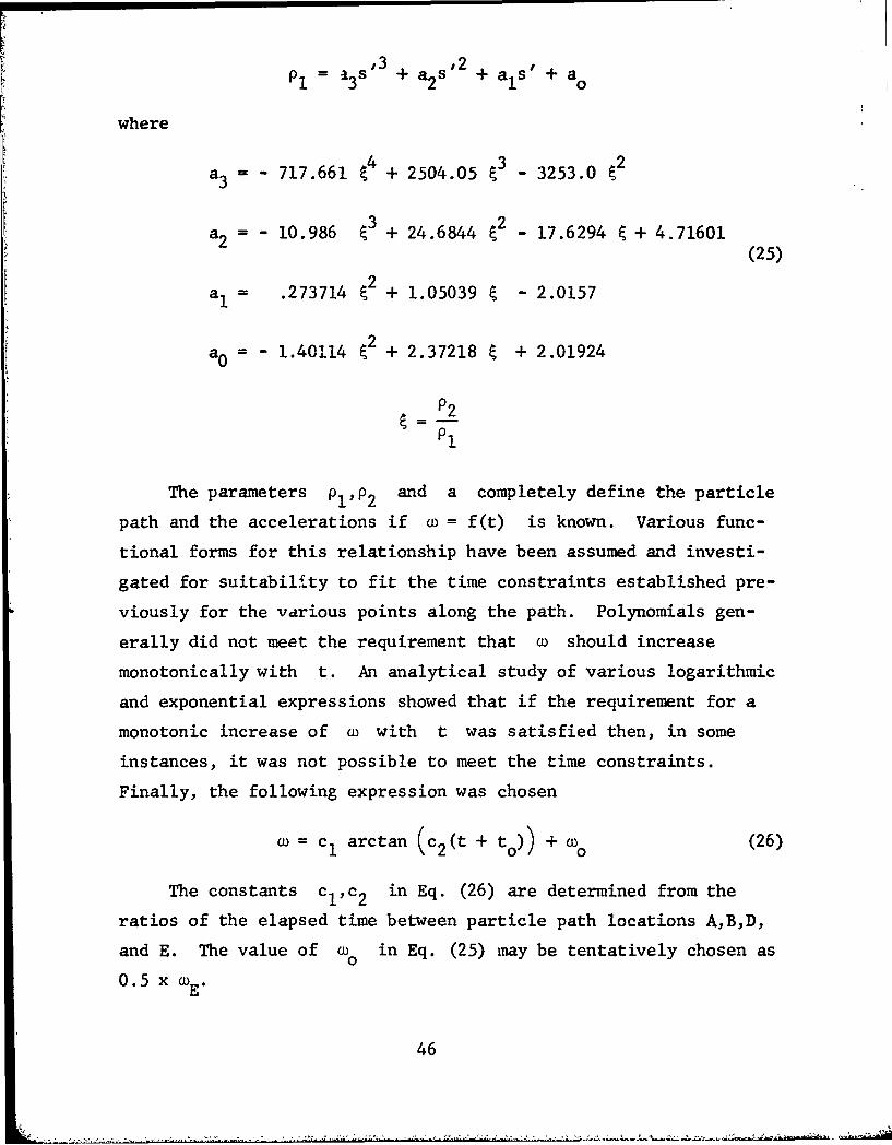
P = '3 3 + a2 s'2 + als' + ao
where
a3 = - 717.661 a4 + 2504.05 a3 - 3253.0 a2
a2 = - 10.986 3 + 24.6844 2 - 17.6294 a + 4.71601(25)
a1 = .273714 2 + 1.05039 a - 2.0157
a 0 =-1.401.I14 62 + 2.37218 + 2.01924
P2a0 .4014 +=.718m +2.12
Pl
The parameters plP 2 and a completely define the particle
path and the accelerations if w = f(t) is known. Various func-
tional forms for this relationship have been assumed and investi-
gated for suitability to fit the time constraints established pre-
viously for the various points along the path. Polynomials gen-
erally did not meet the requirement that w should increase
monotonically with t. An analytical study of various logarithmic
and exponential expressions showed that if the requirement for a
monotonic increase of w with t was satisfied then, in some
instances, it was not possible to meet the time constraints.
Finally, the following expression was chosen
W = cI arctan (c2 (t + t0)) + Wo (26)
The constants cl,c 2 in Eq. (26) are determined from the
ratios of the elapsed time between particle path locations A,B,D,
and E. The value of w in Eq. (25) may be tentatively chosen as
0.5 x wE.
46

Use of the Idealized Particle Path Geometryin the Tire-Soil Model
The analytical expression for the particle path geometry is
convenient for the determination of accelerations. To use this
analytical expression for the calculation of inertia forces in the
7 -tire-soil model it is necessary to determine the constants in that
expression. To this end it is assumed that the constants in the
particle path equation may be determined from the v = 0 case.An alternative to this assumption is that the particle path re-
mains unchanged for small increments of velocity and the particle
path geometry for a given translational velocity would be deter-
mined by an updating procedure. Analysis of a few cases indicated
that, in view of the approximate nature of the particle path con-
cept, an elaborate updating procedure would be justified only if
more experimental information on the geometry of particle paths
were available.
For the assumption chat the particle path geometry may be de-
termined from the vf = 0 case, computations of accelerations
become a simple matter. They require the addition of a short sub-
routine named "ACCE" to the program that was developed for the
computation of tire performance for given tire and soil input data.
(Main program "KTIRE" and subroutine "SLFI," developed for tire-
soil interaction simulation, are described in TACOM Tech. Report
No. 11900 (LL147) (Ref. 4). The subroutine "ACCE" is called from
subroutine "SLFI" after the first approximation of the coordinates
x,z is computed for each nodal point of the slip line field. The
accelerations computed by the subroutine "ACCE" are then used in
the difference equations for the computation of a and 0 and
for the computation of the improved values of the x,z coordinates
of the nodal point.
47

A detailed flow chart of the expanded program for the computa-
tion of tire performance with consideration of soil inertia force
is given in Appendix B.
Problems Encountered with the Development ofthe Computer Program
These were generally of the same nature as with the program
based on velocity fields. However, the analytical simulation of
the particle path geometry resulted in continuous time derivatives
alleviating the overlap problems at zone transitions encountered
with the other program. The critical accelerations occurring at
the singular point, that are inherent in the problem, limit the
applicability of the method to about 10 to 20 feet/second trans-
lational velocity, depending on the tire dimensions.
In cases where the soil and loading conditions are such that
there is no slip line field in the front, association of the vari-
ous points of the particle path with relative positions of the
tire is no longer applicable. Experimental information on parti-
cle paths generated under such conditions is needed for meaningful
simulation of the geometry of particle paths and the motion of
particles in the time frame of tire passage.
Results of Sample Computations
For evaluation of the effect of soil inertia forces on tire
performance by this method, computations were performed for a few
typical cases. Results of these computations are shown in Tables 3
and 4.
In the computations for the performance calculations shown in
Tables 3 and 4 no overlap was experienced for the translational
velocities indicated, i.e., all slip line field solutions were
48

) -
TABLE 3 TIRE PERFORMANCE AT VARIOUS VELOCITIES
Tire Size: 9.00-14
Tire Radius: R = 1.18 ft
Tire Width: B = 0.74 ft
Load: L = 614 lbs
I. Inflation Pressure: pi = 10.9 psi
7 Limit Pressure: PZ = 11.0 psi
Deflection Coefficient: e = 0.9
Slip: s = 10%
Cone Index Gradient: CGR =15 pci
Interface Friction Angle: 6 = 22.80
Translational Pull Sinkage Contact Entry RearVelocity ft/sec Coefficient in. Slip Angle () Angle
0 0.3268 0.724 0.0738 26.06 12
5 0.3334 0.599 0.0614 23.90 10
8 0.3340 0.593 0.0600 23.84 10
10 0.3346 0.588 0.0618 23.77 10
12 0.3352 0.583 NA 23.71 10
single valued. The highest velocities shown in these tables are
approximately the limits above which the solution becomes multi-
valued.
It is seen that the increase of tire performance due to soil
inertia forces are minimal in these cases and, for all practical
purposes, negligible.
49
... .. " "i I " " -- . - ' - " " . .. - l ! i . . - ! l -.. . .

TABLE 4 TIRE PERFORMANCE AT VARIOUS VELOCITIES
Tire Size: 4.00-7
Tire Radius: R = 0.59 ft
Tire Width: B = 0.40 ft
Load: L = 225 lbs
Inflation Pressure: pi = 10.3 psi
Limit Pressure: p1 = 10.6 psi
Deflection Coefficient: e = 0.85
Slip: s = 30%
Cone Index Gradient: CCR= 19.6 pci
Interface Friction Angle: 5 = 27.80
Translational Pull Sinkage Contact Entry RearVelocity ft/sec Coefficient in. Slip Angle (0) Angle (0)
0 0.3217 1.11 0.089 42.3 22
5 0.3270 1.08 0.093 42.0 22
8 0.3291 1.07 0.131 41.9 22
10 0.3508 0.93 0.135 39.3 20
Summary Discussion of the Particle Path Methodand Conclusions
The consideration of soil inertia forces by the particle path
method is simpler than with the method of velocity fields. The
analytical simulation of particle path geometries results in smooth
changes of velocities and accelerations from one nodal point to
another in the slip line field. As a result, the limitation im-
posed by the multivaluedness of the solution of the differential
equations defining the slip line fields is less severe than the
velocity field method, and analysis of tire performance at higher
velocities becomes possible.
50

4i
The drawback of the particle path method is that its empiri-
cal basis includes only a few tests. Therefore, it was unavoidable
to make somewhat arbitrary assumptions in the analytical simulation
of the particle path geometry to attain a usable method. However,
there is enough freedom in the analytical simulation of particle
paths to allow for adjustments should more experimental information
become available.
The most interesting and important result of the analyses per-
formed by the method of partL1e paths is that, in agreement with
the results obtained with the umethod of velocity fields, the effect
of soil inertia forces on tire performance is minimal for the
translational velocities investigated. An explanation for this
finding, that is somewhat contrary to expectations, is that in the
cases analyzed tire performance was governed by failure conditions
in the soil. Even though soil inertia forces affected the geometry
of slip line fields, the stresses in the soil were controlled by
its strength; therefore, soil inertia forces had little effect on
the interface stresses and, consequently, on tire performance. A
logical amplification of this explanation is that soil inertia
forces are very likely to have appreciable effect on tire perfor-
mance if they affect the mode of failure in the soil. Multivalued-
ness of the solution of Eq. (1) is an indication that the soil may
not fail according to the concepts of soil plasticity. At this
time neither theory nor experiments are available that would apply
to the problem.
Another result of the sample calculations worth noting is
that the computed average value of contact slip changes with veloc-
ity. The improvements in tire performance with speed reported in
Ref. I refer to a constant slip of 20 percent. The question may
be raised whether the improvement in tire performance with speed
51

would manifest itself over the entire slip range, including the
maximum pull performance, or whether the observed improvements
signify only an accelerated development of the interface shear
stresses with slip as the travel velocity increased. Tire perfor-
mance experiments at various velocities over the entire slip range
are needed to clarify this problem.
52

4k VI. EFFECT OF LOADING RATE ON SOIL STRENGTHAND TIRE-SOIL INTERACTION
Introduction
In tire-soil interaction the soil is loaded at a rate that is
directly proportional to the translational velocity of the tire.
The rate of loading affects the strength of soil in many ways. In
civil soils engineering practice consolidation and creep theories
deal with the long term effects of loading rates on soil strength;
the .oading rates encountered in tire-soil interaction problems
fall into the category termed as "rapid" or "quick" loading and the
soil strength referred to as "undrained" indicating that during
such rapid loading there is no drainage of the soil. For the pur-
poses of civil soils engineering, laboratory tests aimed at deter-
mining the strength of soil under rapid loading conditions are
performed so as to reach the maximum load in a matter of minutes.
In tire-soil interaction the loading rate is generally faster
than that considered "rapid" in civil soil engineering. Soil be-
havior at loading rates comparable to those encountered in tire-
soil interaction has not been investigated until recently, since
laboratory investigations at these loading rates require special
equipment, referred to as "dynamic" triaxial testing apparatus.
In dynamic tests, loads are applied in fractions of seconds. Dy-
namic tests are generally strain controlled and investigations
relate strength properties to the strain rate,
Indirect information on the effect of loading rate on the
strength properties of soils is also available from various sources
where the resistance of soil to the penetration of plates, blades,
or cones is measured at various rates of penetration.
53

Physical Causes of Strain Rate DependentStrength Properties of Soils
The physical causes of the strain rate dependent behavior of
soils are manifold and some of them are not clearly understood.
The rate of strain affects soil behavior on the microlevel through
its effect on the physicochemical and electrochemical bonding
forces between the soil particles. On the macrolevel, moisture
redistribution during shearing and plastic flow of contacting par-
ticle asperities are the major time-dependent phenomena that affect
soil strength and tire-soil interaction. Since these phenomena
affect the results of the various types of laboratory and field
strength tests and tire-soil interaction in a different way, it is
important to consider the mechanism underlying these phenomena
when strain rate effects are analyzed. In the following discussion
many aspects of these very complex phenomena are omitted so that
the essential mechanism may be clearly presented. For the purposes
of this discussion it is convenient to group soils in three cate-
gories: saturated cohesive type soils, cohesionless soils, and
partially saturated frictional-cohesive soils.
In saturated cohesive type soils, such as the Buckshot clay,
moisture redistribution during loading is the most important single
factor responsible for the increase of soil strength with the rate
of strain. The phenomenon of moisture redistribution can be best
explained by considering a triaxial test (Fig. 17). Loading of
the sample in a triaxial test results in a stress state ultimately
leading to the development of a failure surface where shear
stresses exceed the shear strength of the material. In the process
of straining the sample, high shear stresses along the potential
failure surface tend to dilate the soil. This tendency to dilate
reduces the pore water pressures along the potential failure
54

AHT -
Potential Failure
Surface
H. -\\ _ Moisture
Migration
• dc .AH/HStrain Rate = d - AT
Fig. 17. Moisture Migration in Triaxial Test
surface relative to the rest of the sample. The reduced pore water
pressures suck moisture toward the failure surface, therefore in-
creasing the moisture content locally. Thus, a moisture redis-
tribution occurs in the sample during the test and the actual
strength of the sample corresponds to the moisture content in the
immediate vicinity of the failure surface. Experiments confirm
that moisture redistribution takes place in dynamically tested
triaxial samples (Ref. 23).
The rate of moisture migration depends on the permeability of
the clay. The total amount of moisture that migrates during a test
depends on the rate of migration and the time available for migra-
tion. Obviously, this latter depends on the strain rate and hence
dependence of the strength on the strain rate. It should be noted
that this moisture migration occurs even though the test is of the
55
"undrained" type, i.e., no water is going in or out to the sample
during the test and the total water content of the sample has not
changed.
The process of moisture redistribution is extremely complex
and its analytical treatment would require the knowledge of stress
states in the specimen for the deformed geometry as well as pore
water pressure response of the soil to these stress states. From
the viewpoint of tire-soil interaction, a significant feature of
this complex redistribution process is that the rate of moisture
migration toward a potential failure surface depends not only on
the properties of soil, but also on the stress states in the
vicinity of that surface and the distance from the impervious
boundaries (the sealed bottom and the rubber membrane in the tri-
axial test) of the specimen. These conditions are different in
tire-soil interaction from those in a triaxial or a field test,
therefore, strength-strain rate relations found by such tests are
not immediately applicable to tire-soil interaction problems.
In cohesionless soils the experimental evidence concerning
the effect of strain rate on their strength is inconclusive.
Early experiments by Casagrande and Shannon (Ref. 24) showed a
small increase in strength with an increase of the strain rate,
while Whitman and Healy found the shear strength of sands unaf-
fected by the strain rate (Ref. 25). Larew and Atakol (Ref. 26)
found that the rate of shear strain affected the strength of co-
hesionless soils. These experimental results indicate that the
response of cohesionless soils to dynamic loading is not uniform
and the mineral composition of the grains and arrangement of the
particles also play a role. The strain rate may affect this re-
sponse by delaying the force transmission from particle to parti-
cle due to the inertia of the individual particles and the plastic
deformation of the contacting surfaces.
56

Xs
In partially saturated frictional-cohesive soils the effect
of strain rate on strength properties is diverse. In the three-
phase solid-water-air system pressures of pore water, as well as
of pore air, may be generated and moi3ture redistribution during
loading may be prevented by pore air pressures. Also, if there
are open channels, the pore air pressure may be relieved; the time
lo rate of this relief would depend on the air permeability of soil.
In summary, the effect of strain rate on the strength properties
sag of partially saturated frictional-cohesive soils is exceedingly
complex and cannot be evaluated, even qualitatively, on the basis
Mir of theoretical and experimental information available at present.
Correlation of Strain-Rate Effects in Laboratoryand Field Tests for Strength Property Determinationand in Tire-Soil Interaction
Dynamic triaxial tests performed under controlled laboratory
conditions are the best source of information on the relationship
between strain rate and strength in various types of soils. Even
so, the measured resistance of the soil sample to the applied
loading includes the effects of soil inertia. Only in the most
recent experiments (Ref. 27) has an attempt been made to separate
inertia effects in the triaxial test from the shearing resistance.
In the dynamic triaxial tests the applied strain rate is con-
stant and controlled during the test. Thus, experimental relation-
ships between strain rate and strength can be clearly formulated;
these relationships may be approximated by a logarithmic relation-
ship between strain rate and strength. Figure 18, from Ref. 28,
shows such a relationship for normally and overconsolidated clays.
Indirect experimental information on the effect of strainrate on the strength properties of soils has also been obtained
from dynamic plate bearing and cone penetration tests (Refs. 29
through 31). In these experiments the total force required to
57

CMi
40normally consolidated
Hover consolidated
35
30 -f
k 25-" ''
:j Ave. Water Content = 29.5%E
n20
0.1 1 10 100 1000
Time to 1% Strain minutes
Fig. 18. Soil Strength - Strain Rate Relationships for Normallyaind Overconsolidated Clays (From Ref. 28)
force the plate or cone into the soil was measured at various rates
of penetration. While these experiments provide useful information
on the behavior of the soils tested under these conditions there is
no theoretical basis for the generalization of these findings to
other types of soils. Also, the evaluation of the strength prop-
erties of soils from these tests is difficult for two reasons.
First, the effect of soil inertia forces would have to be accounted
for separately. Second, the strain and the strain rate in the soil
volume affected varies, and, therefore, any observed effect of the
penetration rate on the load is the cumulative effect of various
strain rates in the soil.
To compare, at least approximately, results of cone penetra-
tion tests and dynamic triaxial tests, an average strain rate was
calculated for cone penetration tests performed in Buckshot clay
on the following basis Slip line fields for cone penetration in
58

clay show that a soil volume of a radius of about R = (5 to 6) , r
- - (r = radius of the base of the cone) is affected by the penetration
• of the cone. If the initial void ratio of the soil is e and0
R = 5r is assumed, then the change of void ratio due to the volume
displaced by the cone (assuming no surface heave) is
e -e +1= 24(1 + ) (27)
The corresponding strain is
Ae+ e (28)0
The average strain rate depends on the average strain and the rate
of penetration. For the WES cone the strain rate is
i: vEEh
(29)
where h = 3.77 cm, the height of the cone. For the standard
* rate of cone penetration (3.05 cm/sec)
= .8 x c(sec) (30)
In the tire tests conducted in Buckshot clay the cone index
varied from 16 to 62. According to experiments reported in
Ref. 32 this cone index variation corresponds to a variation in
moisture content from 40 to 33 percent. The corresponding ini-
tial void ratios vary from 1.37 to 0.97, the average strains
from 1.2 to 1.0 percent, and the average strain rates from
0.8 to 1.0 percent sec"I
In tire-soil interaction a crude approximation for the average
strain ratio may be computed by the assumption that the depth of
59
soil affected by the interaction equals the radius of the tire.
For two-dimensional conditions the average strain rate may be es-
timated as
" rr "
(31)R
This formula was used to compute the average strain rate for
the test series on 9.00-14 tires reported in Table 8 of Ref. 1.
For the tests performed at the standard velocity of 5 feet/second,
the average strain rate computed by Eq. (31) varied from 5 to-1
34 percent sec , appreciably higher than the average strain
rate in a standard cone penetration test. For the tests performed
at velocities from 0.5 to 18 feet/second, the average strain-1
rate computed by Eq. (31) varied from I to 58 percent sec-
Consideration of Strain Rate Effectsin the Tire-Soil Model
In the test series on 9.00-14 tires mentioned previously the
soil was characterized by its cone index obtained in cone penetra-
tion tests performed at the standard penetration rate. For the
purpose of model validation, a relationship between the Coulomb
strength parameters and the cone index was established for the
Buckshot clay in Re.f. 4, that was found to yield good prediction
for the tire tests performed in Buckshot clay. le slip-interface
shear parameters needed in the prediction were established by an
empirical optimization technique.
In order to take strain rate effects in consideration in the
model it would be desirable to establish the strength properties
of the Buckshot clay as a function of the strain rate, determine
the strain rate for a particular case, and apply in the model the
strength parameters adjusted for the strain rate. Since the
60

strain rate is not known a priori, additional iterations would
have to be performed in the model for its determination. Also,
the inconsistency of the average strain rate being different in a
standard cone penetration test from that in a standard tire test,
such an approach would be unworkable. Instead, the experimental
' data reported for the test series on 9.00-14 tires in Buckshot
clay were analyzed by adjusting the cone index values obtained at
the standard penetration rate for the variations of the transla-
tional velocity. The cone penetration resistance was found to
1 vary with the rate of penetration according to the following rela-
tion (Ref. 30)
L 0.092I CIS (.Z-) (32)
* S
Since strain rates are proportional to the penetration rate in
cone penetration and to the translational velocity in tire-soil
interaction, the v/v ratio in the above equation may be substi-
tuted by the ratio of the actual translational velocity to the
standard translational velocity in tire tests (5 feet/second).
An analysis of tire performance was made where the Coulomb
- -strength parameters were determined for the CI values adjusted
for the translational velocity by Eq. (32). Results of this analy-
- sis are shown in Fig. 19 where predicted pull coefficients are
, shown against measured ones. Indicated by various symbols are the
- ranges of adjustment factors for the CI values used in the com-
putation.
It is seen from Fig. 19 that pull coefficients are generally
overpredicted by the tire-soil model if adjustments in the strength
properties for the strain rate are made on the assumption that the
- 61

0
4-) Cd 0
r- cd Q
4 H E- ',4- c~4-30 ;-4
P-i -)4 4 ~c) 4-).H-a
(D 0)~ cdr-
4-). -H 4-) 4)0)~ r4-)
00
H- H
H H $Li 4-) 4-)
0 z 0 C
COO
o~t 0C 0x. U0 0 Q)~ a-)
4C) 0\. Ccj E-
rz 4 I 0 a) ca)00 II E3 E ; ) 0 F
. * Ur 0 0 Cd -H-H*'o C'H - -V A20
0
4u@o~jjao TIfld P943TPaJd
62

cone strength varies with the translational velocities as indicated
by Eq. (32).
There are several reasons why this procedure has not resulted
in a better approximation of the pull performance. These can be
summed up as follows:
I. * In the computations for Fig. 19 the interface
friction-slip parameters were assumed on the
basis of unadjusted CI values. These parame-
ters may vary with the translational velocity
I. of the tire.
* In the tire-soil model the soil properties are
assumed to be uniform throughout the affected
soil mass. In tire-soil interaction, strains
and strain rates vary from point to point.
Thus, if variation of strength properties with
strain rate is to be properly considered in the
model, then the model would have to be expanded
to allow for the variation of the strength prop-
erties at every nodal point. This variation
would have to be determined on the basis of
strain rate computations. The two methods for
the computation of soil inertia forces pre-
sented in Sections IV and V lend themselves
readily applicable to the computation of strain
rates. Velocity fields as well as particle path
geometries may be used for strain rate computa-
tions.
The crude approximation of the average strain
rate by Eq. (31) shows that strain rates are
63

proportional to the translational velocity for
the same tire-soil geometry but vary signifi-
cantly with the rut depth even if the transla-
tional velocity remains the same. Thus, an
adjustment in the CI values based solely on
translational velocities cannot reflect the
effect of strain rate on the strength proper-
ties in tire-soil interaction.
Summary Discussion of the Effects of Strain Rate
on Tire-Soil Interaction and Conclusions
Strain rate significantly affects the strength properties of
certain soils and thereby tire-soil interaction. The experimental
information on the effect of strain rate on soil strength behavior
is limited to a few types of soil. The complexity of the physics
of strain rate effects and the lack of a theory prohibit generaliza-
tion of the results of experiments for other types of soils. Spe-
cifically, clay soils saturated to a lesser degree than in the ex-
periments performed on Buckshot clay are likely to exhibit differ-
ent behavior. More basic research is needed for the interpretation
of strain rate effects observed in the experiments.
Theoretically, the most valuable information on the effect of
strain rate on soil behavior is that obtained in dynamic triaxial
tests where the strain rate is constant and controlled. Indirect
information on the effects of strain rate has been obtained from
cone penetration and plate sinkage tests performed at various rates
of penetration. Interpretation of the results of these tests is
difficult and the general validity of correlations with tire per-
formance are questionable for the following reasons. First, soil
inertia effects in these tests are not separated from strain rate
64

effects. Second, the strain rate varies in the affected soil mass
and, therefore, measured changes in penetration resistance reflect
the cumulative effect of strain rate variation in the affected soil
j -volume. Theoretical and experimental research is needed to estab-
lish strain rate patterns for these experiments.
Soil strain rates also vary in tire-soil interaction. To take
their effect properly into account in the tire-soil model it is
necessary to determine the strain rate distribution in the soil.
Of the various ways to accomplish this the evaluation from parti-
cle path geometries appears to be the most practical. More experi-
mental information on particle path geometries is needed to deter-
mine the parameters in the analytical simulation presented in
Section V.
65

VII. USE OF TIRE-SOIL MODEL INVEHICLE RIDE DYNAMICS SIMULATION
In the simulation of tire-soil interaction by the tire-soil
model it is assumed that tire load and travel velocity are constant
and a steady state exists in the soil. With these assumptions the
fundamental relationships governing tire-soil interaction may be
formulated and compared with laboratory experiments without undue
interference from interactions between tire and vehicle.
Another important area in mobility research is the simulation
of ride dynamics of off-road vehicles. In the first generation
-- dynamic models of off-road vehicles it is assumed that the ground
is rigid and the motions of the vehicle are two dimensional. With
these assumptions it is possible to analyze the dynamics of off-
road vehicles under idealized conditions and validate the model
- - for such conditions.
Ideally, in both vehicle performance and ride dynamics, simu-
lation of the interaction between running gear and vehicle should
be taken into account. Even though in the model expansion reported
in Sections IV through VI velocity effects have been considered
only in a very preliminary way, the model may be used to demon-
strate its potential use in vehicle dynamic models. To this end
sample computations were performed to determine axle height-load
relationships for a 9.00-14 tire predicted by the model for the
conditions shown in Table 5.
Figure 20 shows the results of computations for Cases I and
2. The difference between the two cases is in the value of the
assumed drawbar pull. In this case the 100 pounds difference
in drawbar pull does not appear to affect the axle height-load
relationship appreciably. However, in other types of soils,
67 Preceding page blank
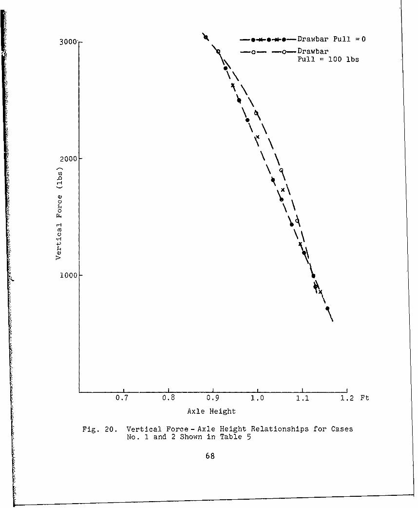
3000- e-..-e-*---Drawbar Pull = 0
300 -o- -0--DrawbarPull = 100 lbs
2000
000
0\
II . I
0.7 0.8 0.9 1.0 1.1 1.2 Ft
Axle Height
Fig. 20. Vertical Force- Axle Height Relationships for CasesNo. 1 and 2 Shown in Table 5
68

STABLE 5 AXLE HEIGHT-LOAD RELATIONSHIPS
K Tire Size: 9.00-14
.. Nominal Radius: 1.18 ft
. . Nominal Width: 0.74 ft
- Soil: Buckshot Clay
Case No. 1 2 3 4
. Tire Inflation Pressure psi 38 38 11.8 11.8
. Limit Pressure psi 29 29 11.6 11.6
Deflection (WES Term.) 25% 25% 25% 25%
- Deflection Coefficient ( ) 0.9 0.9 0.9 0.9
. . Translational Velocity ft/sec 5 5 5 10
Drawbar Pull lbs 0 100 0 0
Cone Index at StandardPenetration Rate
Cone Index Adjusted for 37 37 43 46Velocity
especially in cohesionless soils, it is likely that the effect of
the drawbar pull on the vertical force-axle height relationship
will be significant. Note that the relationship shown in Fig. 20
could be closely approximated by a linear spring rodel.
Figure 21 shows the same relationship for Cases 3 and 4 shown
in Table 5. These two cases differ in soil strength since in
Case 4 the cone index was adjusted for the strain rate correspond-
ing to the 10 feet/second translational velocity. The obtained
axle height-load relationships are almost identical, probably due
to the controlling influence of the limiting pressure that governs
the normal pressure over a large portion of the contact area in
both cases. The soil strength comes into play only in a limited
69

3000-
x Case #3 (v = 5 ft/sec)
O 200 o Case #4 (v = 10 ft/sec).0 2000- 0
oX
iOOO
C)K
C)
0.7 0.8 0.9 1.0 1.I 1.2Axle Height
Fig. 21. Vertical Force -Axle Height Relationships for CasesNo. 3 and 4 Shown in Table 5
70

I. portion of the contact area, hence the almost identical axle
height-load relationships. This relationship is not as close to
a linear one as the one shown in Fig. 20. Nevertheless, consider-
- - ing all other idealizations in vehicle dynamic models, a linear
spring model would be an acceptable approximation.
These sample computations show that the tire-soil model, in
addition to performance predictions, may also be used for the de-
termination of realistic spring constants representing both tire
deflection and ground deformation in vehicle dynamic models. Once
such constants are determined for given tire and soil parameters,
their inclusion in a dynamic model is simple. The main advantage
of this procedure is that in the spring constants determined by
the tire-soil model, the deformability of soil is included allowing
thereby a more realistic simulation of off-road ride dynamics.
71

VIII. TOWED PNEUMATIC TIRE-SOIL MODEL
Introduction
For the analysis of cross country mobility of all wheel drive
vehicles, determination of the drawbar pull that a tire can develop
under various soil and terrain conditions is of prime importance.
The driven pneumatic tire-soil model developed under Contract
DAAE07-73-C0115 serves this purpose. However, it is often neces-
sary to evaluate the performance of off-road vehicles towing
trailers or of all wheel drive vehicles when the front wheel drive
is disengaged or inoperative. For this purpose it is necessary to
determine the towing force needed to move a pneumatic tire in vari-
ous soils.
For the determination of the towing force a pneumatic towed
tire model was developed by Janosi in 1960 (Ref. 33) using soil
parameters from plate sinkage tests. Many features of this model
were incorporated in the tire-soil model for driven tires. Th-3
accuracy of performance predictions achieved by the driven tire
model, the need to use uniform soil parameters in both driven and
towed tire models, and the desire to incorporate the results of
more recent experimental information on tire geometry and interface
stresses into the model, prompted the development of a towed tire-
soil model described herein.
Experimental Information on TowedPneumatic Tire Behavior
Numerous towed tire tests have been performed by various re-
searchers over the years. Most of these were restricted to the
measurement of towing force and sinkage. For the development of a
towed tire-soil model those tire tests are especially of interest
73 Preceding page blank

where tire geometry and interface stresses were measured (Refs. 33
through 40).
The tire geometry measurements on towed tires (Refs. 36 through
40) show that for towed tires the same qualitative relationships
among tire stiffness, soil stiffness, sinkage, and deflection hold
as this general relationship is shown schematically in Fig. 22 for
driven tires. 6
0N
',,'
V
C Large Deflection Small
4 Small Sinkage Large
0
Fig. 22. Schematic Representation of Tire-Soil Behavior(Based on WES Experiments)
74
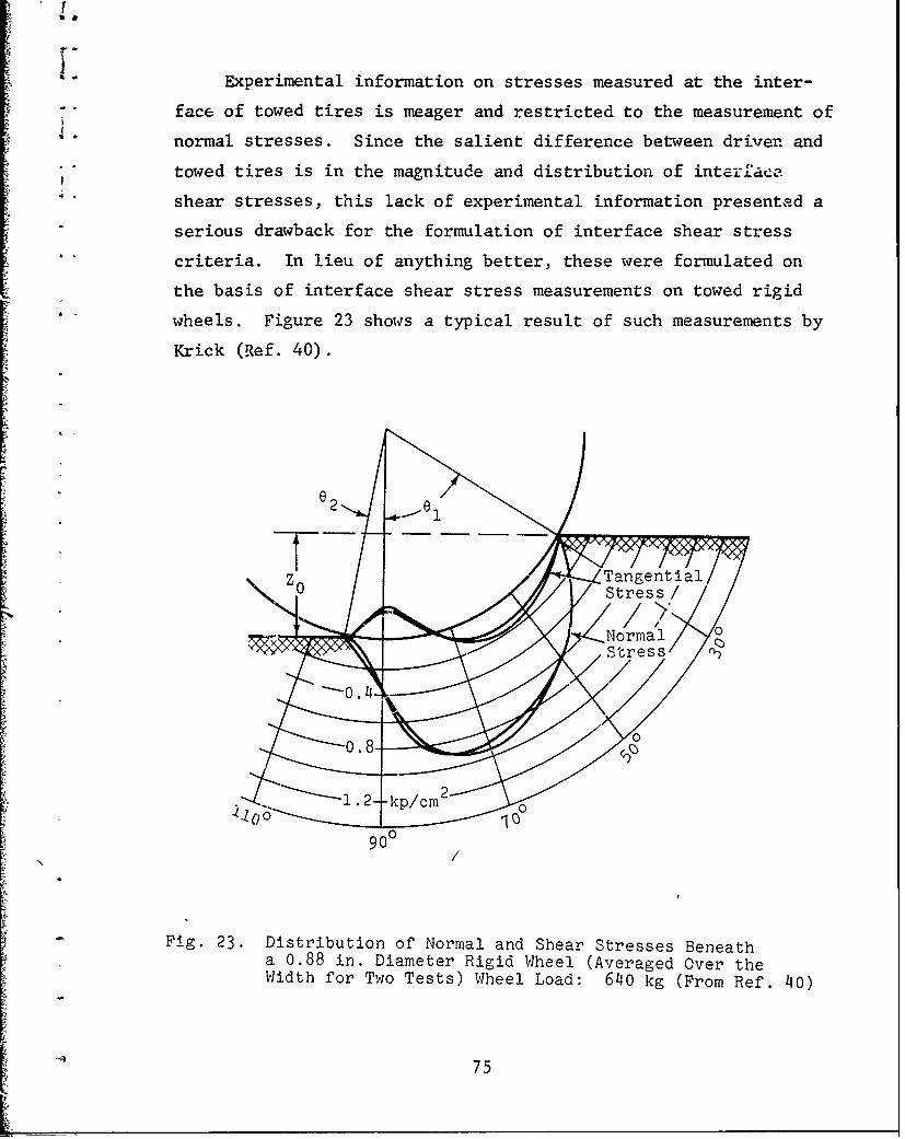
'a
Experimental information on stresses measured at the inter-
""face of towed tires is meager and restricted to the measurement of
normal stresses. Since the salient difference between driven and
towed tires is in the magnitude and distribution of intarface
shear stresses, this lack of experimental information presented a
serious drawback for the formulation of interface shear stress
criteria. In lieu of anything better, these were formulated on
the basis of interface shear stress measurements on towed rigid
wheels. Figure 23 shows a typical result of such measurements by
Krick (Ref. 40).
z0 Tangential
~Normal/ Stress
-o.8-12-.2-• kp/cm2 0
90
N /
Fig. 23. Distribution of Normal and Shear Stresses Beneatha 0.88 in. Diameter Rigid Wheel (Averaged Over theWidth for Two Tests) Wheel Load: 640 kg (From Ref. 40)
~75

Concept cC Towed Tire-Soil Interaction
In the conceptual development of the towed tire-soil model
the inferences drawn from the study of experimental information
were incorporated in the following way.
" Tire deflection was related to the arc
length of the front slip line field in
the same v'ay as in the driven tire-soil
model.
* The interface friction coefficient, 6, that
governs the shear stress distribution, was
assumed to vary linearly from the entry and
exit points to a central angle, o , where
its sign changes. This assumption results in
a shear stress distribution similar to that
obtained for rigid wheels and shown in Fig. 23.
* For the shear stresses the criterion was
adopted that their moment about the tire axis be
zero. While at first glance this criterion ap-
pears to be self-evident for a towed tire where
the applied torque is zero, it should be brought
to mind that in the case of a deflecting tire
normal stresses may also produce moments about
the axis. In such a case the moment produced
by the normal stresses would have to be balanced
by the shear stresses resulting in a different
shear stress distribution. It is in this respect
that the lack of experimental information on in-
terface shear stresses beneath towed tires hin-
dered the development of a towed tire model that
76

would be responsive to this contingency in
shear stress distribution.
For the driven tire-soil model, relationships
were developed between slip and the interface
friction angle. For towed tires, skid or
negative slip is of less importance since it
does not affect travel efficiency or power
consumption. Therefore, skid-interface fric-
tion relationships were not analyzed and
included in the model.
7 Development of Towed Tire-Soil Model
The concepts of towed tire-soil interaction described previ-
ously were incorporated in the towed tire-soil model shown in
Fig. 24. The tire centerline geometry consists of logarithmic
spirals and straight lines, as in the driven tire model. Tire
deflection is assumed to start ahead of the entity point and
*ceases after the exit point. This assumption is incorporated in
the model by the angle a' (see Fig. 24) that defines the end
points of the logarithmic spirals in the front and rear. The
normal stresses are controlled by plastic equilibrium c-nditions
in the soil whenever they are less than the limit pressure p,
that depends on the tire inflation pressure. The shear stresses
and the interface friction angle 5 are assumed to vanish at the
central angle a . A linear variation of 6 from the entry and0
exit points results in a shear stress distribution as shown in
Fig. 24.
For towed tire-soil interaction, the soil model is the same
as for driven tire-soil interaction. Soil behavior is represented
by its Coulomb strength parameters and its unit weight. The gen-
S 77
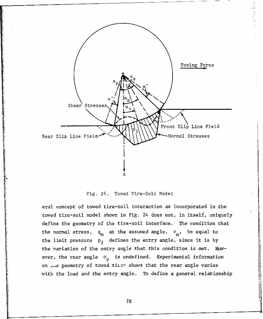
Towing Force
ar
Shear Stresses, OL T
- i Front Slip Line Field
Rear Slip Line Field- °I ..... - Normal Stresses
Fig. 24. Towed Tire-Soil Model
eral concept of towed tire-soil interaction as incorporated in the
towed tire-soil model shown in Fig. 24 does not, in itself, uniquely
define the geometry of the tire-soil interface. The condition that
the normal stress, q at the assumed angle, am, be equal to
the limit pressure p, defines the entry angle, since it is by
the variation of the entry angle that this condition is met. How-
ever, the rear angle a is undefined. Experimental informationr
on L.Le geometry of towed tiftc shows that the rear angle varies
with the load and the entry angle. To define a general relationship
78

for a wide variaty of soil and loading conditions the same approach
was followed as for the development of the driven tire-soil model.
A computer program was written for the towed tire-soil model and
F towing force computations were made for a variety of assumptions
regarding the rear angle. The towed force computations were per-
*- formed for tire sizes and soil conditions for which experimental
data were reported in Ref. 1. These towed tire tests were selected
for validation of the model because soil strength parameters for
the t-wo types of soils used in the tests were already established
in Report No. 11900 (LL147) (Ref. 4).
Since the cost of the large number of computer runs required
to perform the contemplated systematic analysis of the effect of
the various assumptions on the towed force is high, the computer
program was adapted to the General Data Corporation Nova Minicom-
puter owned by the Research Department. Running time of the com-
puter program on the minicomputer is about 4-8 times that on large
computers but the running cost is nominal. Arrangements were made
for input and output data reading from, and recording on, data
files so that results for a large nuber of selected cases could
be obtained overnight.
The computer analyses of a large number of cases served the
dual purpose of comparing results with experimental data and check-
ing on tolerance limits and convergency criteria of various itera-
tion schemes adopted in the computer program. In connection with
the latter, some new problems arose that are discussed below.
Problems Encountered
In the development of the computer program for towed tire-soil
- interaction the experiences gained with the driven tire-soil model
were heavily relied upon. One of the tasks that had to be solved
* *. 79
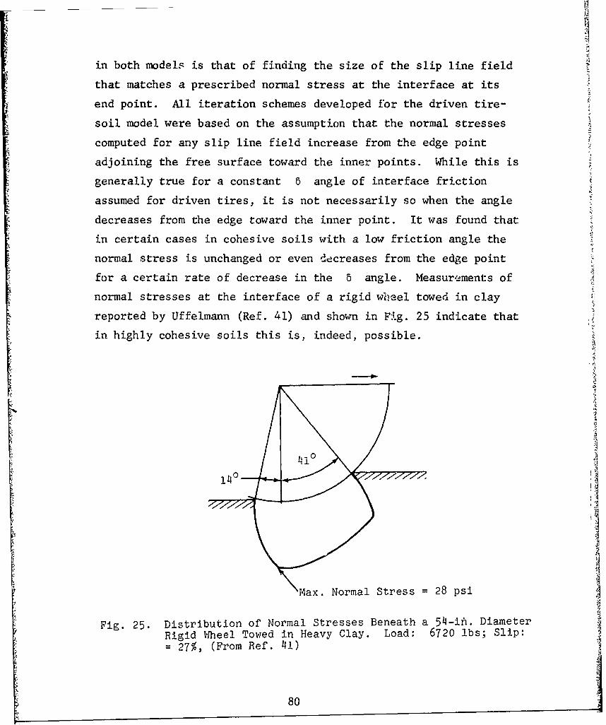
in both models is that of finding the size of the slip line field
that matches a prescribed normal stress at the interface at its
end point. All iteration schemes developed for the driven tire-
soil model were based on the assumption that the normal stresses
computed for any slip line field increase from the edge point
adjoining the free surface toward the inner points. While this is
generally true for a constant 5 angle of interface friction
assumed for driven tires, it is not necessarily so when the angle
decreases from the edge toward the inner point. It was found that
in certain cases in cohesive soils with a low friction angle the
normal stress is unchanged or even decreases from the edge point
for a certain rate of decrease in the 6 angle. Measurements of
normal stresses at the interface of a rigid wV-eel towed in clay
reported by Uffelmann (Ref. 41) and shown in Fig. 25 indicate that
in highly cohesive soils this is, indeed, possible.
14°
Max. Normal Stress ; 28 psi
Fig. 25. Distribution of Normal Stresses Beneath a 54-iil. Diameter
Rigid Wheel Towed in Heavy Clay. Load: 6720 lbs; Slip:- 27%, (From Ref. 41)
80

LThis feature of the normal stress distribution in cohesive
soils made it necessary to make provisions in the program that
U account for this situation. The main problem that had to be re-
solved was the determination of the size of the front slip line
ii field for nearly constant normal stresses. In principle, this
- - problem was resolved by assuming that the size of the front field
I. for entry angles between 30 and 60 degrees is determined by
- - the condition that the vertical components of all stresses be
equal to the load. The rear angle is assumed as 10 degrees for
-- the variations of the entry angle from 30 to 60 degrees. For
entry angles less than 30 degrees the rear angle is reduced by
- -half of the difference between the entry angle and 30 degrees. A
computational scheme corresponding to these assumptions was incor-
porated in the computer program. Results of the towing force com-
putations were compared with experimental data and were found to
- yield acceptable approximations within the limitations of a two
dimensional model.
Results of the Analyses of Experimental Data
The systematic analyses of the experimental data were directed
primarily toward determination of the best assumption as to the
relative positions of the front and rear slip line field controlled
by the angle of separation and rear angle. The effects of other
- assumptions, such as the relationship between the limiting and in-
flation pressures, the value of the interface friction angle at the
entry and exit point, and the location of zero shear stress were
also investigated. In the course of these systematic analyses per-
-formed on the minicomputer over 3000 cases were investigated, all
A representing different combinations of the input data and assump-
tions. The cost of this systematic investigation, if carried out
81
on large computers at commercial rates, would have amounted to
more than half of the contract cost. Even though the number of
cases investigated appears to be large, only a limited number of
all possible combinations of input variables and assumptions are
covered. Nevertheless, it was possible to establish approximate
relationships that define the towed tire-soil model completely and
result in acceptable prediction accuracy. Although further sys-
tematic analyses could have resulted in refinements in the model,
the time spent would have been prohibitive. Also, the systematic
analyses showed that prediction accuracy could not be improved sig-
nificantly unless three dimensional conditions were considered in
the model.
The following assumptions were incorporated in the final com-
puter program on the basis of these systematic analyses:
Initial value of rear angle a = 100r
Initial value of separation angle a = 200
Relationship between rear and separation angle =
a = 1.5 x a + 50 (33)m r
The effects of limiting pressure on the prediction of towing
forces were also investigated. In the case of towed tires the
following relationship was found to yield good simulations
(psi) - 0.82 x p. + 6 (34)PA
The interface friction angle 6 is assumed to vary from a
maximum value at the entry and exit points to 0 at some inner
point. The variation of 6 along the interface is thus defined
by its maximum value and the angle a at which its value becomes0
zero. This angle was defined in the program as
82

a = F a (35)o T m
where the value of the factor F was to be determined by the con-
dition that the moment of the shear stresses about the tire axis
* •be zero. The systematic analyses were run with various values of
the F factor. It was found that a value of F = 0.5 generally
yielded a negligible moment of the shear stresses. Although it
- -would have been possible to set up an iteration scheme whereby the
moment of the shear stresses was made less than a specified tol-
erance by an appropriate variation of the F value, it was found
that the prediction accuracy would not have been improved in a sig-
nificant degree to warrant the additional computer time required
for these iterations. If, however, for any reason, the moment of
shear stresses appears to be unacceptably high, an appropriate
change in the input F value would bring it to an acceptable
level.
The maximum value of the interface friction angle was assumed
as
5max F (36)
In the systematic analysis the effect of the factor F on the
towed force coefficient was investigated by assuming various values
for F6 . It was found that for good simulation F6 may vary be-
tween 0.25 and 0.50. These values are in the range of F6
values evaluated from experimental data on rigid wheels. Shear
stress measurements on towed pneumatic tires in various soils would
be needed to firm up the value of the F factor. A detailed flow
chart of the computer program incorporating these features is given
in Appendix C.
83
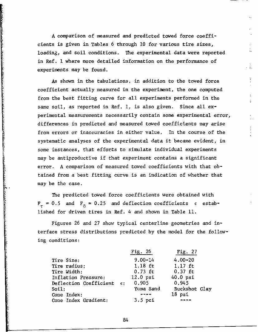
A comparison of measured and predicted towed force coeffi-
cients is given in Tables 6 through 10 for various tire sizes,
loading, and soil conditions. The experimental data were reported
in Ref. 1 where more detailed information on the performance of
experiments may be found.
As shown in the tabulations, in addition to the towed force
coefficient actually measured in the experiment, the one computed
from the best fitting curve for all experiments performed in the
same soil, as reported in Ref. 1, is also given. Since all ex-
perimental measurements necessarily contain some experimental error,
differences in predicted and measured towed coefficients may arise
from errors or inaccuracies in either value. In the course of the
systematic analyses of the experimental data it became evident, in
some instances, that efforts to simulate individual experiments
may be antiproductive if that experiment contains a significant
error. A comparison of measured towed coefficients with that ob-
tained from a best fitting curve is an indication of whether that
may be the case.
The predicted towed force coefficients were obtained with
F = 0.5 and F5 = 0.25 and deflection coefficients e estab-
lished for driven tires in Ref. 4 and shown in Table 11.
Figures 26 and 27 show typical centerline geometries and in-
terface stress distributions predicted by the model for the follow-
ing conditions:
Fig. 26 Fig. 27
Tire Size: 9.00-14 4.00-20Tire radius: 1.18 ft 1.17 ftTire Width: 0.73 ft 0.37 ftInflation Pressure: 12.0 psi 40.0 psiDeflection Coefficient E: 0.905 0.945Soil: Yuma Sand Buckshot ClayCone Index: ---- 18 psiCone Index Gradient: 3.5 pci ----
84
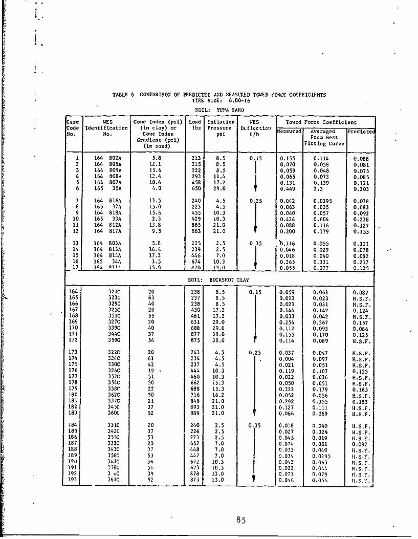
iI
TABLE 6 COMPARISON OF PREDICTED AND .'AST.ED TWED iORCE COEFFICIENTS* TIRE SIZE: 6.00-16
SOIL: YI.NA SAND
case WES Cone Index (psi) Load Inflation WES Towed Force CoefficientCode identification (in clay) or lbs Pressure Dc flec tion Maue vrgd PeitNo. NO. Cone Index psi 6/h FrBest
Gradient (pci)FitnCuv(in sand) Fiting Curve
i 164 802A 5.8 213 8.5 0.15 0.155 0.114 0.0882 164 805A 12.1 215 8.5 1 0.070 0.058 0.0813 164 809A 15.6 222 8.5 I 0.059 0.048 0.0754 164 808A 12.4 293 11.4 0.065 0.073 0.0855 164 807A 10.4 458 17.2 1 0.131 0.139 0.1216 165 35A 4.0 650 29.0 0.449 2.3 0.203
7 164 816A 13.5 240 4.5 0.25 0.042 0.0395 0.0788 165 37A 15.0 223 4.5 0.063 0.035 0.0839 164 818A 15.6 455 10.3 I 0.040 0.057 0.092
10 165 33A 2.3 429 10.3 I 0.424 0.604 0.23811 164 812A 13.8 865 21.0 0.088 0.116 0.12712 164 817A 9.5 863 21.0 0.200 0.179 0.155
13 164 803A 5.8 225 2.5 0 35 .0.116 0.055 0.11114 164 813A 16.4 239 2.5 I 0.046 0.029 0.078 -
15 164 814A 17.3 446 7.0 0.018 0.040 0.09216 165 34A 3.5 674 I 10.3 0.365 0.331 0.21717 1A& A 15 870 13.0 0.055 0.077 0.125
SOIL: BUCKSHOT CLAY
164 321C 20 238 8.5 0.15 0.059 0.061 0.087165 323C 63 237 8.5 0.013 0.023 H.S.F.166 329C 40 238 8.5 0.021 0.031 H.S.F.167 325C 20 430 17.2 0.144 0.142 0.124168 351C 55 461 17.2 0.033 0.042 H.S.F.169 327C 20 631 29.0 0.254 0.367 0.157170 339C 40 688 29.0 0.112 0.093 0.086171 344C 37 877 38.0 0.155 0.170 0.125172 359C 54 875 38.0 0.114 0.089 H.S.F.
173 322C 20 243 4.5 0.25 0.037 0.047 H.S.F.174 324C 61 234 4.5 . 0.004 0.097 H.S.F.175 330C 42 237 4.5 0.021 0.051 H.S.F.176 326C 19 444 10.3 0.119 0.107 0.135177 357C 51 460 10.3 0.022 0.036 H.S.F.178 354C 50 662 15.3 0.050 0.051 H.S.F.179 338C 22 688 15.3 0.222 0.179 0.165180 362C 50 716 16.2 0.052 0.056 H.S.F.181 337C 21 848 21.0 0.292 0.355 0.183182 345C 37 893 21.0 0.127 0.111 H.S.F.183 360C 52 889 21.0 0.066 0.069 H.S.F.
184 331C 20 240 2.5 0.35 0.0.';8 0.040 H.S.F.185 342C 37 226 2.5 0.027 0.024 H.S.F.186 355C 53 223 2.5 0.045 0.019 H.S.F.187 332C 29 457 7.0 0.074 0.081 0.092188 343C 37 448 7.0 0.033 0.040 H.S.F.189 356C 53 447 7.0 0.034 0.0295 t.S.F.IJ 341C 36 672 10.3 0.042 0.063 H.S.F.191 118C 50 673 10.3 0.022 0.044 H.S.F.1921 3 oC 39 878 13.0 0.071 0.079 U.S.F.
361C 52 8731 i3. 0 1 0.04 6 0.056 N.S.F.
85

TAIc. 7 CM-AllSON OF PREDTCTFD AND WA I ER TOWD FORCE COF.FFrCIENTSTIRE SMZE: 9.00-14
fr$ ,SOIL: YIIMA SAND
Case WES Cone Index (psi) Load Inflation 'ES Towed Force CoefficientCode Identification (in clay) or lbs Pressure Deflection Measured AveragedNo. No. Cone Index psi 6/h From Bers t Vredicte
Gradient (pci) Fittng Curve(in sand)
71 164 778A 8.1 230 7.5 0.15 0.052 0.065 0.075
72 164 779A 6.3 225 7.5 I 0.093 0.079 0.082
73 164 780A 13.8 230 7.5J 0.074 0.043 0.065
74 164 786A 17.9 232 7.5 0.026 0.036 0.063
75 164 777A 8.9 460 16.4 0.113 0.114 0.108
76 164 782A 12.4 458 16.4 0.068 0.081 0.092
77 164 783A 5.2 436 16.4 0.216 0.203 0.137
78 164 785A 17.6 460 16.4 0.046 0.060 0.083
79 164 781A 12.1 871 36.7 0.177 0.161 0.123
80 164 784A 17.0 864 36.7 11 0.086 0.109 0.097
81 165 5A 10.7 144 5.5 0.25 0.049 0.028 0.067
82 165 4A 11.2 225 6.0 0.031 0.035 0.088
83 165 7A 22.5 216 6.0 0.028 0.024 0.072
84 165 6A 12.4 446 8.8 0.063 0.052 0.098
86 165 28A 3.5 656 11.6 0.386 0.315 0.201
87 165 3A 13.8 850 14.5 0.035 0.081 0.115
88 165 24A 15.0 862 14.5 0.041 0.076 0.114
89 1-65-64 13.3 156 5.5 0.013 0.027 0.067
90 1-65-65 11.8 144 5.5 0.035 0.027 0.061
91 1-65-66 12.7 243 6.4 0.021 0.034 0.086
92 1-65-67 11.6 237 6.4 0.025 0.035 0.087
93 1-65-68 13.2 650 11.3 0.029 0.066 0.109
94 1-65-69 10.3 821 14.0 0.069 0.105 0.136
95 1-65-70" 13.2 348 7.5 0.017 0.041 0.093
104 1-65-71 9.7 286 6.9 0.024 0.045 0.089
97 1-65-72 10.3 163 5.7 0.001 0.031 0.064
98 1-65-74 11.0 450 8.8 0.028 0.058 0.108
99 165 9A 20.7 243 2.0 0.35 0.074 0.023 0.071
100 165 11A 13.0 226 2.0 I 0.058 0.027 0.080
101 165 12A 24.2 668 7.5 I 0.033 0.034 0.090
102 165 13A 3.7 653 7.5 0.198 0.180 0.195
103 165 10A 12.4 892 10.6 0.044 0.069 0.123
SOIL: BUCKSHOT CLAY
135 297C 17 227 7.5 0.15 0.040 0.056 0.087
136 304C 32 231 7.5 0.017 0.031 H.S.F.
137 308C 54 238 "7.5 0.013 0.022 H.S.F.
138 298C 17 434 16.4 0.161 0.135 0.123
139 303C 51 444 16.4 . 0.027 0.036 H.S.F.
140 305C 32 459 16.4 0.033 0.060 0.068
141 301C 16 621 25.4 0.308 0.374 0.176
142 306C 30 653 25.4 0.110 0.102 0.100
143 313C 57 652 25.4 ' 0.063 0.046 H.S.F.
144 307C 31 866 36.7 0.136 0.155 0.123
145 418C 52 882 36.7 0.088 0.072 H.S.F
146 299C 16 431 7.5 0.25 0.128 0.098 0.124
147 310C 34 436 7.5 0.025 0.041 H.S.F.
148 312C 57 441 7.5 0.034 0.027 H.S.F.
149 308C 16 817 16.4 0.379 0.410 0.254
150 311C 35 867 16.4 0.092 0.086 H.S.F.
151 419C 51 886 16.4 1 0.047 0.056 H.S.F.
152 314C 36 243 2.0 0.35 0.025 0.023 H.S.F.
153 414C 55 225 2.0 0.062 0.017 H.S.F.
154 417C 25 233 2.0 0.047 0.028 H.S.F.
155 390C 40 451 4.4 0.042 0.032 H.S.F.
156 408C 23 449 4.4 0.042 0.053 H.S.F.
157 410C 51 442 4.4 0.023 0.026 H.S.F.
158 409C 22 646 7.5 0.082 0.087 0.161
159 411C 52 658 7.5 0.021 0.035 H.S.F.
160 412C 39 658 7.5 0.030 0.046 H.S.F.
161 413C 39 883 10.6 0.041 0.062 H.S.F.
162 415C 56 864 10.6 0.032 0.042 H.S.F.
163 416, 23 880 10.6 0.127 0.131 0.124
86

- TABLE 8 COMPARISON OF PREDICTS) AND MEASURED TOWED FORCE COEFFICIENTSTIRE SIZE: 4.00-7
SOIL: YI'HA S,.%D
-- Case WES Conte Index (psi) Load Inflation WES Tin , i.aCode identification (in clay) or lbs Pressure Deflection Measureu, Averaed 'redictedNo . No. Cone Index psi '/h From Best
Gradient (pci) FittLng Curvc- I (In sand)
44 16. 198A 17.3 85 16.2 0.15 0.259 0.085 0.06845 164 824A 15.8 106 16.2 0.113 0.117 0.08246 164 825A 9.8 123 33.2 0.171 0.258 0,25047 164 800A 13.0 210 33.2 0.305 0.377 0.175
a 48 164 827A 17.6 121 6.2 0.25 0.025 0.073 0.10749 164 828A 19.6 122 6.2 0.033 0.067 0.10450 164 831A 25.1 185 17.0 I 0.130 0.077 0.09851 164 822A 13.0 216 17.0 0.139 0.188 0.16152 164 829A 19.6 234 17.0 0.107 0.126 0.13153 164 826A 12.1 348 26.0 0.210 0.434 0.229
54 164 833A 18.7 109 2.5 0.35 0.119 0.049 0.10055 164 834A 18.7 152 5.5 0.086 0.064 0.109
sl 56 164 IA 22.8 145 5.5 0.103 0.052 0.10057 164 830A 19.6 224 10.1 0.076 0.085 0.13258 164 832A 19.9 455 12.7 ,0.125 0.174 0.157
SOIL: BUCKSHOT CLAY
21 363C 56 113 16.2 0.15 0.027 0.034 H.S.F.22 368C 45 117 16.2 0.117 0.040 H.S.F.23 371C 26 97 16.2 0.093 0.062 0.07924 365C 46 226 33.2 0.137 0.087 0.07725 383C 66 228 33.2 0.083 0.056 H.S.F.26 373C 41 335 51.8 0.188 0.212 0.12527 380C 66 340 51.8 0.109 0.002 H.S.28 375C 42 439 63.3 0.237 0.427 0.14329 385C 66 451 63.5 0.146 0.141 H.S.F.
- 30 364C 46 117 6.2 0.25 0.026 0.033 H.S.F.31 372. 26 103 6.2 0.068 0.050 H.S.F.32 367C 62 217 17.0 I 0.134 0.044 H.S.F.33 370C 44 229 17.0 0.074 0.068 H.S.F.34 374C 42 330 26.0 0.148 0.122 H.S.F.
35 384C 66 340 26.0 0.097 0.067 H.S.F.36 376C 37 436 35.0 0.287 0.292 0.16637 386C 65 446 35.0 1 0.108 0.097 H.S.F.
38 378C 34 221 10.4 0.35 0.104 0.073 H.S.F.39 387C 66 222 10.4 0.072 0.037 H.S.F.40 379C 36 322 17.0 0.208 0.115 H.S.F.41 388C 66 336 17.0 0.042 0.055 H.S.F.42 377C 38 446 21.9 0.197 0.192 H.S.F.43 389C 68 448 21.9 0.083 0.074 H.S.F.
87

TABLE 9 COMPARISON OF PREDICTED AND MEASURED TOWED FORCE COEFFICIENTSTIRE SIZE: 4.00-20
SOIL: YUMA SAND
Case WES Cone Index (psi) Load Inflation WES Towed Force CoefficientCode Identification (in clay) or lbs Pressure Deflection Measured Averaged PredictedNo. No. Cone Index psi 5/h From Best
Gradient (pci) Fitting Curve(in sand)
59 164 791A 7.5 218 24.7 0.15 0.211 0.198 0.10760 164 793A 16.4 22i 24.7 0.118 0.084 0.06261 164 788A 12.1 426 48.2 0.246 0.252 0.11962 164 794A 12.7 440 48.2 0.227 0.246 0.10963 164 795A 16.1 446 48.2 0.195 0.181 0.093
64 165 14A 27.7 22? 11.4 0.25 0.079 0.038 0.07665 165 15A 14.4 238 11.4 | 0.046 0.065 0.09166 165 19A 16.1 338 18.2 1 0.062 0.079 0.10067 165 16A 13.0 450 24.7 0.156 0.131 0.123
68 165 21A 25.6 233 6.7 0.35 0.064 0.034 0.08469 165 22A 25.6 350 11.0 | 0.029 0.058 0.09l70 165 20A 16.4 442 15.0 0.048 0.074 0.1l1
SOIL: BUCKSHOT CLAY
105 401C 48 305 82.0 0.08 0.056 0.065 H.S.F.106 402C 22 307 82.0 0.08 0.156 0.251 0.123
107 269C 20 204 24.7 0.15 0.059 0.086 0.099108 275C 48 221 24.7 0.023 0.036 H.S.F.109 279C 32 228 24.7 0.048 0.055 0.067110 271C 18 388 40.0 0.255 0.427 0.177111 273C 46 456 48.2 0.070 0.081 0.085112 287C 32 448 48.2 0.127 0.139 0.125113 286C 48 629 61.0 0.097 0.122 0.099
114 270C 22 204 11.4 0.25 0.044 0.057 0.099115 276C 52 228 11.4 0.022 0.028 H.S.F.116 280C 33 225 11.4 0.044 0.042 H.S.F.117 272C 19 377 18.2 0.207 0.171 0.162118 274C 48 450 24.7 0.038 0.056 H.S.F.119 288C 33 447 24.7 0.1d3 0.089 0.114120 281C 47 645 37.5 0.095 0.090 0.099121 291C 40 664 37.5 0.130 0.121 0.125122 293C 54 637 37.5 0.055 0.073 H.S.F.
123 277C 50 211 6.7 0.35 0.03E 0.025 H.S.F.124 283C 29 236 6.7 0.021 0.042 H.S.F.125 289C 19 236 6.7 0.021 0.067 0.11026 278C 50 433 15.0 0.035 0.044 H.S.F.
127 284C 30 454 15.0 0.077 0.084 0.125128 295C 19 421 15.0 0.140 0.156 0.181129 282C 45 651 23.0 0.060 0.078 H.S.F.130 292C 35 664 23.0 0.092 0.115 0.136131 294C 52 628 23.0 0.033 0.062 H:.F.132 285C 52 696 23.0 0.052 0.070 H.S.F.
133 400C 48 660 16.1 0.45 0.055 0.063 H.S.F.134 403C 22 635 16.1 0.228 0.210 0.183
88

41 m 0
r4 0 H 00- 10 ,.
0D 0 0 0
El) UiH -A
z 4 E-1tz4 4-4-
1-4 a)) 4-J U0 0 0
0 PQ4 WOer 0 0 0 )o C0 0 0
IAWr < r 4
0 >0 44
00
14' a% ON -It 0TU)O4 u0 4L~ H 0~
cr3 rU rz--.. t-4 r-4 c') 0 I 4 : C J w 4r-4 41 . . .
I M~ 0 0 0 0 o
En u) 00r ) 0044 NW 44 t-4 rH4 . . .4 Jer- r-4 0 0
0 0) '0 00 A r-4 Lf) 0j r 1 l 0 E4 4
U) -r (d V)-4U C0- - i a; 4 N -4 '00U1 4.1 0 44- 0)r- F4e' Q
U) Cd A ,0 O
H 00 CV) f0 rX
.,4 H 3 N 0 ) 00 10 10. u H 4 . .H
Hd P49 r4-r N -
0 Hn
44~ Co 0 0410 H0 H0 0
89

0
-, ,1000 lbs/sq ft
000 lbs/sq ft
Normal Stresses
Fig. 26. Interface Normal and Shear Stress in Sand Predicted
by the Towed Tire-Soil Model
Evaluation of the Towed Tire-Soil Model
In Tables 6 through 10 towed force coefficients predicted by
the model are compared with experimental data. The soil strength
parameters used in these predictions are those established for
Yuma sind and Buckshot clay in Ref. 4 as functions of cone penetra-
tion values. Considering that the soil strength parameters deter-
mined on this basis are approximate ones the prediction accuracy
achieved by the towed tire-soil model is generally very good.
A review of towed force coefficient predictions was made with
the objective of determining causes of differences between predic-
tions and experiments. As a result of this review the following
conclusions were reached.
90
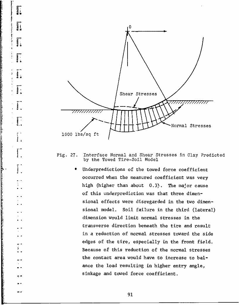
ih 0'4
" Shear Stresses
~Normal Stresses
1 000 ibs/sq ft
SFig. 27. Interface Normal and Shear Stresses in Clay Predicted
by the Towed Tire-Soil Model
!. Underpredictions of the towed force coefficient
occurred when the measured coefficient was very
~high (higher than about 0.3). The major cause
U.
of this underprediction was that three dimen-
: sional effects were disregarded in the two dimen-
sional model. Soil failure in the third (lateral)
dimension would limit normal stresses in the
transverse direction beneath the tire and result
in a reduction of normal stresses toward the side
edges of the tire, especially in the front field
Because of this reduction of the normal stresses
the contact area would have to increase to bal-
ance the load resulting in higher entry angle,
sinkage and towed force coefficient.
91

* Bow waves, unaccounted for in the model, may
also cause an increase in the towed force
coefficient.
0 In cohesive soils, the towed force coeffi-
cient is very sensitive to small changes in
soil strength. This may be best illustrated
by the summary plot of the WES tire tests
(Fig. 28) where test results were plotted
against the dimensionless number
1
N =CI b *d (6\~c W I + b/2d
When N is less than about three, the towedc
force coefficient curve becomes very steep
indicating that very small changes in the
cone index result in large changes in the
towed force coefficient. Under these condi-
tions it would be unrealistic to expect that
the towed force coefficient could be deter-
mined by any method very accurately.
* The towed tire-soil model is based on the
concept that soil failure conditions govern
the towed tire-soil interaction. In strong
cohesive soils, soil failure does not occur
under the tire load and the concept of tire-
soil interaction does not apply. In the
computer program this situation is recognized
by an approximate calculation that computes
the failure stresses for an infinitesimally
small slip line field and compares these
92

0o4oLv Legend
0.35 o 4 .00 - 7.2 - PRo9.00 - 14.2 - PR011.00 - 20, 12 - PR
....o .16 x 6.50 - 8.2 -PRfitI0 3 0 -16 x 11.50 - 6.2 - PR
4.), am16 x 15.00 - 6.2 - PRQ*26 x 16.00 - 10, 4 - PR" 0.25 < 31 x 15.50 - 13, 4 - PR
1.4
001 0.20 O
0
r2 0.15 A
o0E- 0.10 A
1 0.05 -
0 2 4 b 8 10 12 14 16 18 201
Cbd 2 1" "W 1+b
Fig. 28. Variation of Towed Force Coefficients with NC in
Fat Clay (From Ref. 1)
with the limit stress. If these computed
failure stresses are larger than the limit
stress then no failure occurs in the soil,
and therefore, soil failure is not the con-
trolling factor in tire-soil interaction.
The computer message for this condition is"use hard surface formula" indicated by
"H.S.F." in the tabulation.
93

In the towed tire tests on Buckshot clay,
hard surface condition is frequently indicated
in the predicted towed force coefficient column.
An examination of tLese cases showed that in
the majority of the cases the measured towed
force coefficient was in the range of 0.02-0.05.
Since the rolling resistance of tires on con-
crete or asphaltic surface is in the lower limit
of this range, the hard surface designation
appears to be appropriate. The measured sinkage
in these cases is very small indicating that the
soil actually behave-d as a stiff rather than a
plastic material.
Tire-soil interaction in these cases is
governed by the deformation rather than by the
strength properties of soil. For the simula-
tion of tire-soil interaction under such condi-
tions, the soil model would have to be modified
accordingly. Since this situation is not criti-
cal in off-road mobility the development of such
a model was not a.tempted.
94

IX. CONCLUSIONS AND RECOMMENDATIONS
Methods have been developed to estimate soil inertia forces
- - generated by a tire traveling at various velocities and to take
these inertia fo. :es into account in the solutions of the differen-
tial equations of plasticity for soils. These methods have been
incorporated in the computer program simulating tire-soJi interac-
tion. From the analysis of the effect of soil inertia forces on
tire-soil interaction the following conclusions were drawn.
As long as the inertia forces generated in the soil by the
traveling tire result in single-valued solutions for the front and
rear slip line field, the effect of soil inertia forces on tire-
soil interaction is minor. At a relatively low velocity (in the
range of 10 feet/second) solution of the differential equations
of plasticity becomes imltivalued indicating that soil behavior
must be different from that described by plasticity theory. The
effect of such stress states on soil behavior is unexplored and
cannot be analyzed by present state of the art methods.
It is recommended that both theoretical and experimental re-
search be started to gain insight in soil behavior under such con-
ditions and a theory be developed that could be applied to tire-
soil interaction at high speeds.
In tire-soil interaction the rate of loading of the soil and
the rate of strain is directly affected by the velocity of travel.
The strength properties of certain soils are appreciably affected
by changes in the rate of strain, while other soils are relatively
insensitive to strain rate variations. The increase of soil
stre.-gth with strain rate is probably the major contributor to the
improvement of tire performance with speed.
95

Strain rates vary in the affected soil mass in both tire-
soil interaction and in the various field tests used for soil
property determination. In order to approach the problem of
strain rate effects in a logical way, it is necessary to develop
methods for the determination of strain rates in tire-soil inter-
action as well as in the various field tests.
Strain rates are directly related to particle path geometry.
It is recommended that methods be developed for the determination
of strain rates from particle paths and experimental determination
of particle path geometries be extended to tire-soil interaction,
cone penetration, and plate sinkage tests under a variety of soil
conditions. More experimental information on particle path geome-
tries would also be useful to improve the computation of soil
inertia forces in tire-soil interaction.
An important new concept, that of the contact slip, was de-
veloped in connection with soil particle acceleration determination
by the velocity field method. This concept establishes a relation
between the shear stresses at the tire-soil interface and the mini-
mum value of slip that is necessary to develop these shear stresses.
Slip that exceeds the value of contact slip is a waste in energy
and tire wear.
It is recommended that the theory of contact slip be further
developed and general relationships between contact slip and inter-
face friction be established. It is also recommended that in all
tire tests the horizontal displacement of selected soil particles
at the surface be routinely determined and compared with the mea-
sured conventional slip value. The horizontal displacement of a
soil particle at the surface is a measure of the contact slip. Its
measurement is a simple way to obtain experimental information that
could lead to economies in off-road vehicle usage.
96

A towed pneumatic tire-soil model has been developed that
predicts towed force coefficients with good accuracy. For improve-
I, ment of the model it is recommended that tnree dimensional condi-
tions be taken into account in the model. The consideration of
* I three dimensional conditions is also essential for the prediction
of towed force in the case of dual tires.
* 97
I'
4. 97

X. REFERENCES
1. Turnage, G. W., "Performance of Soils Under Tire Loads," U.S.- Army Corps of Engineers, Waterways Experiment Station, Techni-
cal Report No. 3-666, Report No. 8, September 1972.
2. Crenshaw, B. M. and Butterworth, C. K., "Aircraft Landing GearDynamic Loads from Operation on Clay and Sandy Soil," AF FlightDynamics Laboratory Technical Report AFDL-TR-69-51, February1971.
3. Crenshaw, B. M., "Aircraft Landing Gear Dynamic Loads Inducedby Soil Landing Fields," AF Flight Dynamics Laboratory ReportTR-70-169, June 1972.
4. Karafiath, L. L., "Development of Mathematical Model for Pneu-matic Tire-Soil Interaction," U.S. Army Tank Automotive Command
Mobility Systems Laboratory Tech. Report No. 11900(LL147),July 1974.
5. Besdo, D., "Principal- and Slip-Line Methods of Numerical Analy-sis in Plane and Axially Symmetric Deformations of Rigid/PlasticMedia," J. Meth. Phys. Solids, Vol. 19, 1971.
6. Butterfield, R. and Harkness, R. M., "The Kinematics of Mohr-
Coulomb Materials," Proc. of the Roscoe Memorial Symposium onStress-Strain Behavior of Soils, Cambridge University, March1971.
7. Soil Mechanics-Selected Topics, edited by I. K. Lee, AmericanElsevie'" Pub. Co., New York, 1968, "Theories of Plasticity andthe Failure of Soil Masses" (E. H. Davis).
8. Hill, R., Lee, E. H., and Tupper, S. J., "The Theory of WedgeIndentation of Ductile Materials," Proc. Roy. Soc. A., Vol. 188,1946.
9. Mandl, G. and Fernandez, L. R., "Fully Developed Plastic ShearFlow of Granular Materials," Geotechnique, Vol. 20, No. 3,September 1970.
10. Roscoe, K. H., "The Influence of Strains in Soil Mechanics,"Geotechnique, Vol. 20, No. 2, June 1970.
99 Preceding page blank

11. Shield, R. T., "Mixed Boundary Value Problems in Soil Mechan-ics," Q. Appl. Math., Vol. xi, No. 1, 1953.
12. Spencer, A. J. M., "A Theory of the Kinematics of Ideal SoilsUnder Plane Strain Conditions," J. Mech. Phys. Solids, Vol. 12,1964.
13. Karafiath, L. L., Nowatzki, E. A., Ehrlich, I. R., and Capin, J.,"An Application of Plastici'ty Theory to the Solution of theRigid Wheel-Soil Interaction PIcblem," U.S. Army Tank Automo-tive Command Mobility Systems Laboratory Technical ReportNo. 11758(LLi41), March 1973.
14. Karafiath, L. L. and Nowatzki, E. A., "Stability of SlopesLoaded Over a Finite Area," Highway Research Board RecordNo. 323, November 1970.
15. Karafiath, L. L., "Plasticity Theory and Stress DistributionBeneath Wheels," J. of Terramechanics, Vol. 8, No. 2, 1971.
16. Nowatzki, E. A. and Karafiath, L. L., "Effect of Cone Angleon Penetration Resistance," Highway Research Record No. 405,1972.
17. Nowatzki, E. A. and Karafiath, L. L., "General Yield Condi-tions in a Plasticity Analysis of Soil-Wheel Interaction,"J. of Terramechanics, Vol. 11, No. 1, 1974.
18. Karafiath, L. L., "On the Effect of Pore Pressures on Soil-Wheel Interaction," Proc. Fourth International Conference forTerrain Vehicle Systems, Stockholm, April 1972.
19. Janosi, Z., "An Analysis of Pneumatic Tire Performance onDeformable Soils," Proc. of the ist Int. Conf. on the Mechan-ics of Soil-Vehicle Syster 3, Torino, 1961.
20. Wilson, N. and Krzywicki, h., "Soil Mechanics As it AffectsVehicle Performance," Canadian Geotechnical Journal, Vol. III,No. 4, November 1966.
21. Yong, R. and Webb, G., "Energy Dissipation and Drawbar PullPrediction in Soil-Wheel Interaction," Proc. of the ThirdInternational Conference for Terrain Vehicle Systems, Vol. 1,
July 1969, Haus der Technik, Essen, West Germany.
100
22. Windisch, E. and Yong,R., "The Determination of Soil StrainRate Behavior Beneath a Moving Wheel," J. of Terramechanics,Vol. 7, No. 1, 1970.
23. Whitman, R. V., Richardson, A. M., and Nasim, N. M., "TheResponse of Soils to Dynamic Loadings," MIT Dept. of CivilEngineering Research Report R62-22, June 1962.
24. Casagrande, A. and Shannon, W. L., "Stress Deformation andStrength Characteristics of Soils Under Dynamic Loads,"2nd Int. Conf. on Soil Mech. and Found. Eng., Rotterdam,1948.
25. Whitman, R. V. and Healy, K. A., "Shear Strength of SandsDuring Rapid Loading," Proc. of ASCE, Vol. 88, No. 2, April1962.
26. Larew, H. G. and Atakol, K., "The Effect of Rate of ShearingDeformation on the Shearing Resistance of a Cohesionless Soil,"Sandia Laboratories Report SC-CR-67-2658, June 1967.
27. Yong, R. N. and Japp, R. D., "Stress-Strain Behavior of Claysin Dynamic Compression," Symposium on Vibration Effects of
Earthquakes on Soils and Foundations, San Francisco, ASTMSpecial Publication 450, June 1968.
28. Richardson, A. M. and Whitman, R. V., "Effect of Strain RateUpon Undrained Shear Resistance of a Saturated Remolded Clay,"Geotechnique, Vol. XIII, No. 4, December 1963.
29. Truesdale, W. B. and Nelson, R. D., "Soil Tests and SoilResponse Studies," AFFDL Tech. Report 70-169, Vol. 11, June1972.
30. Turnage, G. W., "Resistance of Fine Grained Soils to HighSpeed Penetration," Report No. 5, Technical Report No. 3-652,U.S. Army Engineers Waterways Experiment Station, June 1973.
31. Turnage, G. W., "Resistance of Coarse Grained Soils to HighSpeed Penetration," Report No. 6, Tech. Report No. 3-652,U.S. Army Engineers Waterways Experiment Station, July 1974.
32. "Strength-Moisture-Density Relations of Fine Grained Soilsin Vehicle Mobility Research," U.S. Army Engineers WaterwaysExperiment Station, Technical Report No. 3-639, January 1969.
101

33. Bekker, M. and Janosi, Z., "Analysis of Towed Pneumatic TiresMoving on Soft Ground," U.S. Army OTAC Report No. RR-6,March 1960.
34. Murphy, N. R., Jr. and Green, A. J., Jr., "Stresses UnderMoving Vehicles - Distribution of Stresses Beneath a TowedPneumatic Tire in Air-Dry Sand," U.S. Army Corps of EngineersWaterways Experi-ent Station, Technical Report No. 3-545,Report No. 5, July 1965.
35. Freitag, D. R., Green, A. J., and Murphy, N. R., Jr., "NormalStresses at Ihe Tire-Soil Interface in Yielding Soii',"Highway Research Record No. 74, 1965.
36. Trabbie, G., Lask, K., and Buchele, W., "Measurement of Soil-Tire Interface Pressures," Agricultural Engineering, November1959.
37. Smith, M. E. and Freitag, D. R., "Deflection of Moving Tires -
Centerline Deflection Studies through July 1963," U.S. ArmyCorps of Engineers Waterways Experiment Station, TechnicalReport No. 3-516, Report No. 3, May 1965.
38. Freitag, D. R. and Smith, M. E., "Centerline Deflection ofPneumatic Tires Moving in Dry Sand," J. of Terramechanics,Vol. 3, No. 1, 1966.
39. Krick, G., Die Wechselbeziehungen Zwischen Starren Rad,Luftreifen und Nachgiebigem Boden, Dissertation, TechnischeUniversitat Munchen, 1971.
40. Krick, G., "Radial and Shear Stress Distribution Under RigidWheels and Pneumatic Tires Operating on Yielding Soils withConsideration of Tire Deformation," J. of Terramechanics,Vol. 6, No. 3, 1969.
41. Uffelmann, F. L., "The Performance of Rigid Cylindrical Wheelsin Clay," Proc. of the Ist International Conference on theMechanics of Soil-Vehicle Systems, Torino, 1961.
102

APPENDIX A
COMPUTER PROGRAM FLOW CHARTFOR ANALYSIS OF EFFECT OF SOIL INERTIA FORCES
" ON TIRE PERFORMANCE BY METHOD OF VELOCITY FIELDS
(Pages 11, 20, and 24 omitted)
A-1

I~lPAA. AJTOPLOP CPAP? SET FLOCSAPT F-.92 LISTING PAWE PG
CnAPT TITLE . INTA3OUCTOPV CCMEN"TS
S&IR POOGPAM
VIlS PROGRAM COMPUTES TIP! Cf4IVEt 15
C'dTPv.IpTZPFACE SERESSES AND PEP~oMANCE
PAPAMETERS FOP GIVEN TIP! CSARACTEISTICS.
SOIL SV*FA.GT. PAOPEPTtES WIT". CONSIDERATION
OF SOIL INEPTIA FCESI GENERATED AT VARIOUS
VISE TRANSLATIONAL VELOCITIES.
TH! PROGRAM CONSISTS Of FOUR PASTS
SUBROUTINE! SLFIA
I "U' V AARES Apt, READ IN.! PeAN
PROGRAM PR DATA FILES IN TI.! FOLLOWING CODER
APR (EftRY ANGLE IN DEGREES)I
APR IsFPAPATION ANGLE IN DE!GA.sES
PA INORINAS. TIRE DIAMETEP IN FEET)I
SO (ICAIN4AL TIRE IOTI" IN FRET I
to (LOA IN LGll
P0 (LI SIT PRESSURE IN PSIl
OE (DEFLECTION COEFPICIENT EPSILON)
SL (SLIP IN DECIPALI
Si (SLIP PARAMETER J ZevDI
SPA (SLIP PAPAPITER El
C' ICOAESICN IN FPONT FIILO.LRS/SRFVTI
CA (CO"ESIONI IN REAR FIELD.LPS/SSFTI
FR (EPICTICN ANGLE IN FRONT FIGL.OESEtESI
(PICTirN ANGLE IN REARPFIELO.OE!0EESI
GF (UNIT VEIGN? IN FRONT FIftD*LR5/CURTl
GA (UNIT REIGN? IN REAR FI11LO.LPSCUPTI
AS (ANGLE ADDED TO MITRY AND REAP ANGL TO PARE
ENS OF O4EP.RCT 105
AR (WFAR ANGLE IN OEGREFSI
TNTRT.REAP.ANC SEPARATION ANGLES APE' TO PE
OSTAINTD PROM III? STANDARD TIRE-SOIL IN4TFPACTIOA
PROGRAM.
DESIGATION OF RAIN VAIAtS IN TIE P3RAM AM!
AAD ENTRY ANLtE IN RADIANS
AAR SEPARATION ANGLE IN RADIANS
III PETS COEFFICIENT FOR LOG SPIRAL
01 INTERFACE FRICTION ANGL! I0ELTAI IN RADIANS
PL LIMITING PEESSURE IN tMSIFT
A-2

A-A.AI Uf*PLO. CPAR? Set PLOC,.ART FPHAI LISIIAG, PAGE 91
NO DEICOAEO TIRE RADIUS
PW COPUTED LOAD
Ayr CCAAJTED 00Pa"A PJLL*IT TOTAL TONGUE
1.45 TONote Poom N.4AL. STRESSES
SkA SI4AGE
("4I CPNTPA. AN4GLE AT P0,14 . IN DEGREESshe 001.4 NOPMAL STPESSE AT POINT H IN LGS/SOVT
- - IAt.., ACOO 1.4T OP PTl W IT" 1PEPEAESCE1 TO IRE AS1
4 MYII OOINATE OP POINT W IT" PtPEENCE I TPef AS
SAVWOTAPE SAPIA
THIS SU@POUTIHE COMPUTES COOOUATES. SIGMA AND5vw THETA VALUES FOR SLIP LINE PIISOS
T DESIGNATIONS1 OF WAIN VLPIA.EfS APE
AIIJ) A COORDIATE AT POINT I.4
fo1.it COOPOINATE of rot.? 3.4
1,3.44 SIGNA AT PO14T I.j
*a T5I.J1 T-fTS AT POINT 3.4ACCAIt.JI A COMPONENT OF INAERTIAL ACCELERATION
'1~ACCOII.jlI7 COMPONENT OF INERTIjAL ACCELEATION
G4 4PLITIONAL CONSTANT
* V QII .4, A COMPONENT OP VELOCITY
UIlI 2 COVPDWNT OT VELOC ITY
a Jii TAAG).4 OP CETe.IN4E AT P01NT
0(4 DLTA ANGLE ATOINT
THIS SU9PVOJTIE COMPUATES TAE VELOCITT FIELD PON
31LIP LINE FIELD GTOAErTtIs COMPUTED IN
lsUJTIVE SLFI.74
DESIGNATION4S oP AVE MAIN VA) [email protected] APE
S - UA(I .44 A CONVOAAPT OF VELOCITY AV POINT 1.4Utfl.4I r COMPONENT or VEL.OCITY A, .0OINT 1AJ
LJ(I*J VELOCITY COMPONENT ALON4G J LIVE
Ait .44 VELOICITY CD3A0Po"ET ALONG0 ILN
SA.4POJTtNE ACO..
- V~TS SUIOCj4TINE COMPUTES TOE ACCELERATIOS AT LI .4
AN
A-3

1101*WTOPLOW COART OCT FLDCHAR? FPWKS LIST104 PAff 03
CKANT TITLE IN""L~ TWy C*NeNTS
POINT Facm VELOCIT ICl OtTISNINPD IN us UeuIWV
v COW.
IMSI6NATIONI OF TH *AIN v*RIAR.I!S AOL
VTOAWS TRULaV 20444. ILOCITY
ACCXI I.JI X CONP0NNV OF MASIS? * ACCtE'AyICt
£CCIIJl Z C0bo..I~ 0, INERIAL * ACCUIRATION
A-4

18104/6 UAUTOPLOW C0APT SIT rLOCHAMIT OINKI LISTING PAGE 04..
CIOAPT TITLE 2COU ES
0 S. I16 ----------S oT C IO7rI og I ooooo0ooI IC 1 1o0oos5o0 2T
I R T9 TOD-* NOI 0! 7 C3 * C I I ITE TO '0 EV I I - wEI1TE TO DIV /*~~C 0113 9 D1 I // '
* * I AEC * 0.01145329 I I VIA FORMAT 1 I VtA i CEEA
* 20 J * I. II * OE.P /00000500•I NOTE I? I 00000440/I 01 04l[ l. I.i .....
IG I I *LIST LIS 1 GOO a- LIS" L.S* - -- ...... I I - -.. ...... 4•• I. . . . A SNO
I 03 I II I I I e • eeI.I. . I I I I
0I I ACCEII.hJ) * 0.0 I I ooo0o00lo0! 30 I ooooo00S2/I SN I- I I I ............ I. . ........ I /C21O0°40II 201
I &CCZlIJI * 5).7 I I I • I I / AElTE[ TO 0EV • I )... . .. .*.......... . I I .............- - -II /• *I|S
I8•/1I I EI.2.I41e094II oI I I I -m~ I2 1. 1 I I E.4 E0 I
I ~~~ LIS S I, SJ.I/ EOTI LST
It0 O* P I --.. .. . . .. .....-- -- . .. . ... I A 111.o III I A 1 AI11I 0 1o/5.1 I 0 1I s .... ... ...I
, I------ - - - -I **,,;,;V-,: 12201 240 I *CZIi 0) 1 1 .0 T~ a, A00 tI A • ................. A I -- - - - - - -- - - !
- b DOI I I I VI 0 I9 SO I 3I I I 1 LIST A. o. * 1 ....... . .. . .)
4 • * • ¢o14 Ti LLI1 I[II . :. L!0 ST!
1 1 1 I 0 1 L C 1 P I I I
I I 000001011 20 I ISA.. ... ... ... I I - -I . A.. .0.O .3 I
LO0000020A 2 1 l TO EV L•.';IPO I I5Lt* S/TAS I
A I *"LP IP S I II . A0000 IA 2• ........ I
I n • ISI- - - - - - - - -0 • I
- - I I A . 70I15I.3I A * *E *3 I A I2 - I WRITEI, I*I
I t-. I V I IOO [ 41 AAN*A C*AEIN -
I I A I ------- -I - - I I2 / I II 0 0 5 I COMPUTE I ALEI
* IT T A T I I I P SEPARATION ASGLA
I / 'OA . I / U I E I T I /0000 A7A0 I 33I
END OF I I A I I 10)I I E.IE 2
L AS toAPE AE I [Ti I A I IA EIE4A 230
II I 0000 0/I 24I I 0 72 -
/000000O0/ 2S C.......... I.I.II I I - - - - - - I AI
4 I SITE I m- 0 1I IcAA /2 - 40
.D t -.. ..... . ........
S 0I I IOP I IT EI I /I O VIAUE 1 34VIA ...... PONA .. ... . (, 1p OZ- ...... .....
II II IT IICI IS0000S1 I II! 24 I S N
I 4 * 0 * I 1 0 * a 5 . 0 1 4 I VI NO .A I I I M S
I .00.. ...... A I NLI..P.. .- I E-- G 1-1
tI I t
.... .. 40 00T0I IU .. .. . . .L I 1
I .0 I ..
C .p. I I *I •I q l LIST "*000071'11 - II
es I
1 /00061.1 as1[ t C AAWRI I+A0
1 1/
:" OFl DATA L0 0 10000401 IS txI ts PN• T.sEl LISTE I 1 IOS
114)~ ~ 1t 1 tt of il&f i [10 I~s I 1 .10•00 6•0.1!
A-5
A I I I I A
I I /00000Sl1 O TE 26 11O1A42
A. .. . . ... ...... IL .ly ...... 0...4T 94
4) • I •A . A 1" . I A . . .) .
......... * .. .... T U 01
•~~~~~~ 9.01 /00lOI $
+ • • I IT N I -*+11 PN AXI IA -5

I,~4.JOLO1 CHART SET fLOC ART FI41NK LISTING PAGE 01
CPA14T 13T.E P43C!001421
AF'04.34.- 1. ----- --- ;--O000081 Onl 0 I 9 1 09
I SI * 91441 3 3 3 I H• .... • IZ ! SLPIA 1
o I I I04.34 ... I IC I
I Al ASIMIRII I I II I I I1 1 -157.3 9 3 /0000|0301, 14012 30I I I A !414 .1. ..1 303 5 3817.3 I I at"f11 00 LOOP 1I 0I I I I :! 1
IIII I I
I CC. CO I I .
I I ;0110.0: 0 14
10 01 03 1 111453 D* I C010FI I II.........NO. I
I I
3 021- I I *------ "1 32 1
I
I 3012300 .1123 4 - - 1
I IO , 0 0 1 Ac II.JI . 0.0 1 II A. A I/ 1 I I I - --- ------- I
...... .......... I I I
Ol I 3 I
lo3cSCoe'loo 06 1 1 1 1 3 3
Il I 1| T42 o*i *
I
I... ............. A I I II 0 A I
I sic PStijlu I I *.- -8 or000 14I 3 I OP1 1• 1 I
I 14~314 115.' 31 14I 3
Si%3 SI.P I Ives I
3 432 * 5G1423 I 370................... ys
II
3 III II
/1010 3 00 II 3 I
GU(o 14
( 002010310 3 I
I 330 .............. /14 34
3 I
I .U0IC. 3 I I 14 A1 33 C T r I 1 0 OE 1oDo
I LOOP
.... *. 1---- --- I Ives
I.. Iooltol l
II* • TII
Io l t trN I II
I 1 3 1..
1000901 , 0 3 3 1WIEY
300 09 / O 3 0.. .. .... I 30
* ~; AI I / VVAI F"A sA
T R U . I Io 3 10
A I
I I I1 000011010 41 ?2
tis I2O 1 I~~N II C-.. ... . 0.- . ... ..........
3.11 or 3 3 34193 . .
I I
C T FRON SLI I
I - ---- ---
3 0
C2 -PU ----341SLI----.---~~1
I I,
A-6

II.CLA AUlOP .OB CNMT SET ILOCrABt 'NI LISTING PAGE 06. €&PT TITLE PVO:!ODUPf S
i " " .............at 11 /
At T AU to
A .. o. I A•STONE O4TA Fr.L' Pat., ASlFL.O A AI
Ii
. . . . . ... . .. A
III Va * UIJJI) I .
I III tI Iq WIB III I / 6*31......... . .
I Z9 NU I / 6TO oy I"I/ VIA 'rONmA T /
S4N2 . 37 - l I 118 6.................. .. " ft.V TMP LIST /S...............
I I
.7 A .o 000030so/ NOTE 12BEGIN 00 0OOP N *.* ** *NN*
S, * lI N NO. 36*N*.S LN BNB....^.,.:N A
0............II II CA I
IN-VINI . NTI1 . O OUTE SEPARATIONI NI l ANGLE Poo REAR PIELO
I I C4LYI OOIN * 00(37 I I
I 10000137Ti 13
....... **...........11 VVV 141 VV( 37 1 1I EENI OI? I I...
COMPUTE BETA POI BCANI PFI;D ONL.Y" " IC€€€14o/1 05
k u; l U T*/00001390/I 1Ix s I I. ..................
IN.... ...... . IAIIr BEE.AAB/2,AAN.
I I /57.31
110 * C06 BEN I
N A O COS(A | I
M a' 00 B I sIAN * ILOOP NBE,.1LA/O
N ~I/00001421/ as
I A NI B N PAL SE
M N IGT. NVAX.JcccN0oljIf~ NOTE 0?
A nut I----- 06.ION-l.
it...... . .NB I91 0I I I EN N NINOIAAN)
... ... 0001.20/ It
N I I I r mo * OSIA III ...N... I I.. is.. . . I.. . . 5
I CNI I0 N - -
I U(Nl N I I LETS' N 5
I I N B /O0O0INBO/I lB
6 . . .- YN ~ I"" ... .. ..N
I I
I :X I I I
S10
• 1 A A*00 ** is
I~~ • PXlT•I
I20 .. Ill
A-7

2214/24 AJYO,I.OW CHART SET - V2.OC" "T P12 LISTING PA4 6?
CP.1 127rT.! OK POCTOLUPES
2120 0
... ... ,. .. . ,
I 22 0 * IuS 2
I I t •ut 0u02,2i
CO4PUTT OfLA.ETI%? I I t.. E 'OF MEAN -I!LC 2 I PSI - II €0 T I 4 I'I'I I I
I 0 . |I •mf l a, au
I I I I I
I .. a.............P,
002 *- 00/51.3 /00091/
2 AO - 05/24.1 2 SI! P02/10J2l
I 5A*EKPj.S2*2*AO0 I I I 2 pl. ,PIO T.12.0 II i o 7. " IP I I
I I 2 SIGI - SIG-*ElI l~ •A 1 I I2 Zt/CO1JIA*0 2) 043 i 2
................ •JI0 lF
L 2 0I0200 2.?,22 1
TO POIToDIVE NtID' UT IItISj!P T" I / 0 .. O/ ...... ........ Ie16 I "OTrC It
OIII • I I Cl •csol au S I I COTIU ,2 I - -22 2 22.41 DC00 *I2u * 00 CI • /2 2 2 0 2 NOTE 29*
OC0S180/ 03 -.......--------- 2--.....
II2 2 2 ILIMIT SSEOS12 TMOO 2GT. G2*00001770/• II 1
I . P . ,+ - x lOI 2 2... Co. 2
/C0CI.E./ OSL 2 2
[ F A L S E * 2 I
ONL SITU I
I I t4 EGo.
.0 LOO0
I ... I • A20
l •................. . I * *I I I10I.. . . . 1 I H C FALSE ' P l1.
SC6 ON 0. T 2 0 0. . -.......... I 0 E .
I~ v .f- g
I 2U 2 9 Z 0019/ 2 I 2 i * - 2*3
01 D I I2 VALUT2 P 2O *FAR I I
2 *. . . . .4 2G2*
2 2 22 .00.
2 L1 t 1-------- -2-----2-
I FrC P I
2 1 V.2$ -oO 2fA 2 • 2
I IL- ?,
I I 1 22I 2( Cc*4 NOT t4 12 0 I
2il 2 . I '*2.50X0 • * | IH2
.......... I 2 --------2I 5 A 0A2 2I. I4
2 2 /0000400/2 22 2. .... -- 2 20 2I 2 2 *.......-. 2I CC¢0 CC 2 2 22S? I NOT
fit
31/04,A AJOOPLOW CO AO SET - 'LOCMT FI."e LISIZOG PAG" 08
CrePT IV1.C apoccotpeS
3I a
@3 3oNOTO 0- I t
0 . . . . . I II £ 3j~ 1 4 4m'l*l[ *A . 171 - X9 *I, I
I I AS - SORTCAseet I4COOIY0T CAPtTATIONSF. -M" .AN FIELD TOo ... . . .¢[ G0 ATLS REP. frlogC0A t0O .o....... . !A-IS
100s960/| 03 1 US : .3*Sto lN3) I
NI - M2 4 31- III I3 S* -- j I 3
3 2 I V4 • 1I
. ...0 N......... NINA . . 3 I /00303 SS14 3 3 83" 0 3 I 3 irU(N - 5 |1) 0 |
Nl II V VI- 3I 0 0 C I N I .1 O T N 0 4 I (..e ... . e. ..o .
N............. . i T /002023 30, toW - ----- * - - -00- - -3
.. . . .. . . I P
....I. I .. ...... . . . .3 3 V I I U I I to - 1
.... ........ I I ISA - 0 IU U3*I-$ 3.TI. 3
II 1I1 I I 9000 3N * I I I I
I 3 UUINI •* SIIm N . I I I /3( ON * II U ANC(U 5$13I3I 3
I --- - 000 9 ------ I T II I . . .. 3-I
°° '91" U°'A ' !
I I 79
I ~ ~ ~ ~ ~ ~ ~ ~ 4P *- - - .IV. V I3. 3 3 U OM(S CiI
+' ,,ooozolo"I o, 'c. , p~ Yost"" 1
I N I - oooNIm o .o... ... t I I A----
) c I t I . .9 -. ....I i 3 ( 3 3 I ' 010 0/ I OI NO 9 1 /0000'IN00 332 3.
LO 0 2 9 0 --- I 82stt I
-- 9 * I IIIOUVS (N I . tSNH)I I 3 I 8S t3 t 2 IUI, I 3 .... . .. 3
3I 10 12 1 MR I"I11t I1 1 9 U.U ;;;*-.-I I 90 I
X, f V600lil t3•
I W I I vuk : 1 1 1 . .tV I f.53 3 3. 1 3 Acs" I9 1 3I N3 I" v I I 0 I . UUsill I I I I
I I I I I I I I ITIwO 1 I I I 3 I I
I I• /O JUI.O~f l -
SI -I9 - I I I Y A& SINCIII I30.0 I_------- - ------
I I Nv( 3 11 I e
160 I C 3 9 I 3
]~~~I .4 3AiHI
...... .LI.... .3 ..
,+~~ I NuGIAt -N'rUI I-lPC 10¢ 4 . I I
T L . P I 2 .. . . .
IS Y3 I Y6 II I 1 1, S - It . V3 I
.9 i
I 83.0 I I I I
A 39UI-? I
• ~ ~ I ...................
3 S9. 3 I 3 3 3
IN R INTERFACE 1 0 It
S T R E S E 0 I 3
/ 000I02120^1 1 1
*-------- 9 ... TAo S9I39
4 9 909 -.0 -I
I At •VI - X9 I
•..."..........I A'S - SORtTIA3 e*2 ,
3 6t~ I< I i'...................
.....................
A-9

AMJOP. CPRT SET rLOCHAST PWsl LISTINC PAGE 09CHAPT TI3LC PC!pL ow ro
61o28--- 3.I
Itno .
WH a 1>0 A* 4LN F0 * N
* LOO 0 3
Irs ." a.
I
/00302520 . .------- 0 - /I 00 - I/ ~ ~ ~ 1 1P~ 0co/ I 000024 60/I 39WRUITE 10 De, A..........
/ 6 / , t IflIT(SS4002.1
/ VIA 100 NAT I ITIA J 3/ 23) -s I
IA I*7. 0 A S - SO0TVfl? I
OTTa
I CI I IlS"OtSUA. . 00002620t1 NOTE 30 I1 3 1 POSIN(I61 IUtU! ~~U(N4l I I A . . A . . 0 A A .
- --- u------- I * II- ...................I t *i i e
I "00000-02011 .Is
ICI7 I I I / 000220o1l 20A
. .... 00.
..........• 2I /Oo Iog I 1*o . *SncoSI.l I
I •/WOITEIo q0 / I*1 V .40O / / I
A INO 0. 00 40 t V14 PONIA?LOCo A I a Sotoo0. 930
000 /• I 0000uSo,. 28roc. THE LIST I
IE I 0 11
I r t I If .110. 1 ....................
I /00002,..0o NOTe 32 * : **
/.I C3 I I I I I S g• €O0S~e~l (' I'ALt CTT MOM•VS4
. .. . . . . S 3 0 0 0 0 2 6 6 0 i 1 3 1 1jI ItSHKl I I --- -- - g
...... ............. I I TNgo/I V ITE TO O V •I
I61VIA 'rOWAT
I 2 0002044,T
* I ITSI/ .... .... 'O- THE LIST ... . . . ..lrE O DI 3/ 3 ---- -'CTOIT fl26/ WIT
I
I at
I t 0
I OS
+ '
.t Pxo r
I I o
I - III0
/ VIA P o / I
i wo ° .. D 0... ..
CAL 9X IT
Jr/05A- 10S. *RRRRlce
I /• 333 ,
I I NO0TE 05*+ I NeO*SR •Ne *R.
I niR S N N 0I. 3 I4 9
I ........*..
II -? I O0/0RITO/ S EX /
I /ti 0 /O• o 1 I
I
I $9" 000NRRt
I q) I I
I
7 N N C
-" I A-II
I

a10CA, CJOPI.O, $l - LOCHAT FRCl I I W.f$ PAG! It
TILI s*AGO~ S,.,eI*T KlOt SOUTIE L:I
.. ....
IMCI~0.- Is . .I €c I000 1 t t-. ............... .-........... .... . . ..
-- .... ....... 0031 a$0 I--- -- -- -- to .OO T ' "*
*15-- - m -t'IN * a I "~la * 0 I a* I I --o* l
- J I* I0- .10,I 11I,
IC OI J) - 0 I a
, aJ.,. OR I S 3 0 * T a -
IOVL9OS.1aa a
• 3C atI o .o ' * a a "a~ AN. • a0 .a *. ... a, * ***.
, , a , - t* I ) I • ia a.. ...... ...I NI
I-6 t o I wIca
0 M2* • •... ..... *.....-.....* a . a . .*~o/0
06001aa as
aI o ~ - a .l a a *o,
'N wO I 7 ILa * * a I ESTIVATE L DISTA"Ce
I ACCIRlI• Jl......... ~O
PASSIVEIt GIl aa a a.. a *VP I*i* a O
0 000430/a II a
. ......... ...
a a laaJa * 0 I * . I a ... **. . ...... * I 0*07.. *I IP$ • .ll)
I • /006007I/l I
a a aaajl.@ a I Ia* I 0. 4I al *a 1 I SAF1 s *A; A;og Ia aaJa'C a /io.~I a a a* aa........ *.o I
a$1SO*m*., T .**TIIIJI 0 -ALlC A lS*g~la a . . . . . . . . . .a I IA O A N T * T. .
aaaI
aI a ToNaSaxl a I I aI wugaaa . .aoa... . . ... a
a o A I t a0a aa aa0 h a a a a"~4 0. Do , o,-; .. a a .. ' a a... .. . . .. aaL a . -I I *OlAX a I I , ....
aV9 a a ACOISCOSgll 10a a1II aa O I S(aaa 1 021 -aa,/2a , I -* -- ----a I a N N 0 1 at ---a-a--- -a
a a a 'a *3.14159 1 a............ a A ------ Ao.,aa a
03a a a a a a a aa a a a GG - 32.2 1I a a.a...Ta..
103 O il I
40
* a T
a a a a-a a a* a a a a 00 .g/ * l a a O a I a* *Pg0 b 0 a a 1a DA a a a Iw
L R IIALSI tat IaSa -a + iwN -a a a .. . aa-e. 0 a
* . a........... . .... .. a a * aJ . 1 Ia aa . * aIaIs a /03
000.t0/a as I * a |Ia~oa *a /.5!00670,1 .... 1 .000040/1
11 aA It t Iorl ITo Ue
a I
aa a a at 'I/ ,ist • a aeJ * I aI
!lF,a 2IL/IAN. a)
t0010I4I/a I I a~ a0 LOVI a a 39/0*000a
X0. I
SaaI + OO a a 3 vs. rAiNapaa a a ... .... .. xlt
IOtj. a a III --------
I Iaa.................. a0,. . . .. . ../1 1...Ia 0 S aa-
.a....... ..... a
aafa.. aa a ' .. a--* a. --- a Na. at a a a
I I 1 9 O 0 DIDI 0 Ill410 5 5.........- *... I . 1. 0 . 1a ja ••I a a • a
*a C jal a a a Oa a a 0 T SOQqwlsa oaJa • a a • DN aOao~a, at ..zg * Na lJ •0 a l as *0 Ofaao,.a SaIPC a
...... ~, , a aD yes
a0 a .. ...- /00000710/Ia, NOTE 2 a
. .. ..........
. . . A- 2... . 0 a4 . - .!
I /
/13.01
A!-2.2

-13I04/4 IrlOPL ¢ T SET - ?LOCAIRT PNO LISTIING PAGC I3
ClANT TZlILE S UTINC SLPIA
12.2t.. 1;----- --- DCOMTF TTA AND I .......... ..
*• O TFTI+FA AM +...................•
53 $GM~ AT $1NMULAN I I NPI - V * * J I
10000:101 IraTe Ol 1PEGI 0 LOO3 I I
N. 3 IN PE[GIV 110 LDIol • IO I.N.. N, +1 I I
CO-MPUTE OI0NATS.SIGNA ANO TIETA
4 V. II VLUCS 9I 02 I NOOA. POINTS OF VlIP
I A---- I LINE F11OI I J. I I I- I I I II I Al * I I I 000011*01 NOTE 0I I I I *N N N. NI A N N . I 11CIN 00 LOOP
I I II• I 1 ISI I N N
or I I 0 I N *11.04 - 1
-------- - N I I 5
.I I C. I0 AI t III - VIINIAt I I NONIN - m3 A II I ANDI/AN.I 1 1 A
I I EPOI T.i . t1 I I ALE*I+ I3I .12.
3 3 000tIII 03 I 32
........ .. ........ .
I II I I I• .I1 e
T I -- 11 11 -111I -11 i
141 A.D A .: ..........* I IO I• , ,
' 1 I tO A ON I I• 1
I N NI II Nl P I 0 t ITII4. *I Ioo p W$ N I I |I I1
SEND 0 00N LOOP * I TO YI. I
P P I I 1. - U IP P I I II •*IllI * I(3h4 - 33 3
lIES I N - - -IVE I ........ ............
II II I" I S0001 tooll 13
I I 10IO0010101! 003S.................SIIOOOOI, 1 - N I I t - si*5 - 31
I 0N * IJAIOIP33I) I 11.INS(I.4 - II II I I II
-I al I(302"N 0" N- I I Iu 01l4 NI I.11NCOSIDI) es I I U, I. .III
I EmI
I I I U00001s1011 3J
I .. I I .. .................
A ---- 1 1 V I8" . II I I I.J1INVP
0 00 0O0 I V , 1 4
N- - ------ N~ I I PS II I
I 4 I I 3 I I N" 1. -l I
N ----------- I flAYs II I . .. . .. ... ... ..I I I
/000030 11 NTE 07 I i
L NoLOOP .................A2.00 . l . NAIT3 UNt I O0l3:I I• N N N N N N N N N N* I ZNTIS II.I4 I
I I I I3NtTII. - 33 N I1.0?. I t I I 031 - 3.J3NTI - I
I so I I 1.3 33 41. 1 I IlS---------N .I.....
is 0 III .I tJ I 3/
V.
A- 13
~I0

I Cl'041 &JTOVO0 CAA€ I Sy . PLOCVApT -WI LISTI PA44I I
CA1 TITLE - SLUDO*UVI SL'IA
11 11
I .*~ I
I VI 1..I1.I
I ,J
I VI
I 8 I
I ... .. . ...........
Ie)(0 Ie'. I
00023100. 0 - -
ol VZ * V/IVI V I*A
*~41 l.
IVIOVIZII . I j .J -I
. .ZII. , .! .- I.
I1 Ij tiJf
Is it
V * V
I
II
-000O011. 04 . .I . I ..............
I • Tew I eII #O OvwV I
I V6 V .. V 1 . "2
I . ., . L ,I 1 50 Tq[ LIIT /
i I[ SAI I
.. .. . .. . ]. m I.. . . . . . . . u, a:r .. .. .. .. .. ..
I s, I 05, OT Ia
M" .......
I IJ) L (li.,J)j
6 4 a l l I *N) )T e
I * &CCI(I.J)GGI
:;+ 8I GV .I.t*0I ACCZ| *j J|/G
I VI.6V. GVV?5
I
I
/0000ISOi 0?VVI /OG00ItGV.TII
VLA VVIVIII , *I000II Ia,,, I I |
I VAVICIIyJ- PlO I ( I V IV qI lI I I I V I~ ~ . . . II I I fVooo 3oo/1 oFJ .
o* " "" /O0014G e |
I II I .JI I I V(/ VllJ! TO CCI 7II.J I I ) I I 5511/
................. VA . 41I llJ I l I
/,"* ........
I I
• IS*O.. *5
A-14
22.'94/9 *AUro2PLOW CHART S11 * (LOCMIt9 11492 2.2SIW PAG4 is
CHAT TITLE 5U2*9LTI.2 SL2
14.21 2 2i~0 11•.1"
1•|-)
--- -- --
d 20 O-O2IAO I
* -|. . .211 9 20 2 2
A.$ 'I R.T sI
I , e000o06.o
13
*.." " "2.1 ..0 TRUE* 6
I .0.. . .do of 2. 2-- 1.19 3b22
t I n I t 0
I. 0 I IS
t 2 I I •09 R . I
2 I t0o0030,2 I2tJ6 * * (|2 2 10 2
.............- .-- ..
t iT 0 I o
2O1 F*jS *192072.J - I -to .2 2 I 2 I 262 2J2 ?2.i2 22| 42O - $oJ 9- 2
2 I 22 2?~l 2 34I2- 0
I *20 I 0I I222 .
-dJ 1 S,2211 J ) 11 1• 1 A................ ----- ---- ----
i 2 .0ll0 ll2 2 1 oJ0-
41 •
/200029700. Of
I s $1J SI I TRU
I I IG .10 - - - -- - -- -I Kl
.2 .... .... 1 to.2, 0 1e$112*I.* 1 1 .4 . 2I 0
I I I LIIG•l
2 I* 1 9 2S I I • I 2 2 2 * - *
l • •( *0 o. . ..... .... ........... Il
I0023o 10 1 IPA••13 I
- • ... .. ... ... .." •• k ... .. .. .... .O .... ........ ..
2 2 i 2 I I NOTE to
1.$ 1A UA 0 1 l • t im = • Yl
97 2292 2 2 0'l'N * Gil •2e2 * 2.0•
. ...... .... .2..2..
• .. . - - --- *. 2
I0
I 2o* 0
I S
i20:14.02: 11
2 /000024- 0/- 7
U I 02 02 *! ?SJ 2 0 2 E
2 2 .. le.20 I- - - -I 6.2I20 *3 2 22|
- 22 -29 * . 5.2.?. A TU 9 9
* 2-•*.*1* 200 2
2 2 .. 000- - - - -.
" A -15

3104 i4 £JTOOLO CHART SET - ILOCMA6? F33 LISTING pA6 36
€lMAllT IVLE 5UIOPOUv I N St.WIA
312---I 3-.-----I . , ' J. I -. )/+00037;01 03
I II AT 3jGI GI. t
..... ........ 1 0 *PALfI I G7 .GT. AI$ .......
/00001700/3 023 *
I t t ~ I* . 3* *" 3 * lO IT6 I0
* 3S 1. 3
I I l~ ;I
I II .. I ....... . to IIPALSE I I "- .
I ..........................
1 3 3 3 7 13 3 6 3 3
/O0007O ,0, 033 03J3 * 03333 I3 * I3 3- O00I33A3J3 . 3
TRUE 3 43133/1* -
3 - x 3GI - I * 01.3£%3
I CAJ - 144llOCill
-I -------------
I ISo0000|leo/ It
.........-..... I . . . . ......
3 .......... 3 3
•. . .. . . 1 09'EI 1CI233338 3 X 0 I i
............... I6'5 . VSC 3 30 3 000031P7O/l 3
I I * 11 - 0 2 - I--3 T 3 733.- 6333 - 33 3 3 3 "Plll 3, 62- 3
I 6 - UK " t0 - t I Ali I t3 l 23 3 23 - 3.J - 3 II 3 i 3 3 * 333 * I
I AA83 23 333-- -------- ---------3 .. .. . . .. .0 .. . . . ...3 . .
I I II I I1 /100000199011 14100001790/ 06 ...............
• * 3 3 3 04 1 1 T I. - I3 t
'AL- 3 3eo 3 33*74143 3 TAJ * TA13A3J33I I
I 3 3 3 - t/7M0 1 I
I 3!I
3
I 1000019i40f:1 i
......................
3 373379 1 3 I Z3 - l7. 1
3---- -- -----------
A * 3 I
I 3 3 3)33 * 0 ... .. ... . 4 ., ... .. ... .. .. 3
I 06
I 33Z. 0 3 3
S.3.....
3 3 17.01
' A-16

3 3/04o/1* Av.o PL0* C sAT SET FLOCHA*T F00* LISTING PAGE I?
€1NAOT TITLE SU11MOUfIW LSA
4 - i00*7106*- 01' 0 S00- - - - -N 0-- - - -
S .. .................
1 2 3 3tl. - iAr[ IF "Ne " I*J t
IIj .4 1•3 23.43) *3 3f - * 4 *.T*? N 0
I t * 2 - It I
3 I°
Xt0LJ*2 • *
3 o I .06./COCC002C/3 02 I *,
1 3 0I 1 390
I GV * .0 1 II ACCZ .jI/GG I0000*190/t 12
I I! I *" Nv T3 02.6 Grit 3r
* •
I * TI lE
I V4 3 GV606 0 3 GH3 I C-3 . ............~.......... ....... . l& .035).
* * . 140 A 2?
/000200/ C3 I * *............ . I IFALi * *E YI
Xllj II.T. N
I LA ZO 4 • I I
•~ U! " "$(I 1'l.S .*1*1 .Jlo033T3. Jl I 1 100001200/ 13. tl" I3. ) ... I Ito
3 I3I3 T -
..... .. .... I 11000021100 toA .0* * il1 * I I 3 P I •
I I.JIs US G0 0/ I33 3 **0*I I . LE *3l cat+J 1-9* l
01 .Ol• UAfO(Jh.FII I I* 06 : LI - *SOL. o
................
COM3UTE H3SL AN I 0 *3If
A 2.4 .* IU 0 t I 1000022100 1. *
I NT ccll I [• •ee
3 33 PAOC* T3* * 68)33-* -i
/€0001001I OS 1• XX .4e, 2 0•-•
I0 hJ * I IL - 0 TU
EIO~~JI .Cec l I 1*e 0CI L.I
3l~ 3 2l * 268l J * * 3i-*
I I CIIOAJ III ... * . II 1 3 2 2 0
11114- ll*J .. ................ )........ . ... • IIIALSE[ 1*ll
3 *0000150/ - 00 1 -00022210/ 14 I * I
tOONIEPPAC I I lot3I 0 0 3 *00
f 3i ,* j L , C t P L . 0 ** -- - - - - - - - 3
/7*00C070/3C 053 0 00*TIO e .02. 2 *'€0 3 0
.. ......... I 0 13 ~ ~~~~ t33 332 0 I36 0 3
1 .... 3 2 It ......... . .. 520I CHI 4 3 • I .. I *I I0
I "ii 34 1734c" 3 3 • 0 *e 3 I... .............. . I 3 c I ... S.GTP
3 IIJ 0 0**** 0
/I I
I I
........ 3 1..... A3 *30S
............. . . . .-- 3 .7 36 - •3**. .0PL 00. . .O
S1 0 30 13
I3 AN 3+eb I 3 • 0 0 •
3 ll• 7 H I 3 3 22.1 T 3 3303 p.35.3 3
3G4..00234 3 3 3... 0 9.
............... ...... 3 Jt *0.3 I* * 3 04,
0 * 0 0 *
326.82*01 210
.. ;,3.. 2
3 A-1

ls, A ~AUTOP*OWiI CHANT SIT - FLOCHAAT F*RM LISTING RACE to
CHAI? TVlf - SIR)*UTtIe SLIA
3.. . .....
...
4Tl--
| • J . *N 4-.•
10'0 0 0 3 30 . T R U E
* * 76 IP U *
J JLTT.. mt
A 3 3 .04o* 4 3 3 *.
i• Lf 17.110-11 1
3 39
3P • -- I
3 .06. 3 . .9... . . . -.... 3 9AIN. ¢M$ 33 3
L"4LCPI'CK FfOR MATCH IPtwIo p'otlT OF ILI*LI-NE P3CLO
0 3
3 .. Tu
C4 0 3e
;4. . 0
I~ ADJUSTl~l I
I • I
.• Lt. .. ..............
.CA € -4 .02 .• •
• 4 I I ALI1
O 404.ST L'
,0306+340/ 04 20
08&3c as046/ 34K~
...... ........
• I ... ... ... .. . . . . - ? 1 • . *
4344 - *01+3 0 llS 3 04 3• . ..
....
t I
0 30 3 ... 20
, / . . .0 1 . ... 0 .I.T J I00C30I 0 1411+ I 3------ -- 0.. . ---* - - --3 3.ie4.4.13 0 34 3.IX 30
0$.*... -.... o°
3. .- 33I3
X 0.3 * 9. 0 tI 3
+0300030/ 01 6*0
II
A &o JASt18

|1]04ev4 AUTOPLOW Cl-SPT SET - FLOCMEAT IS LESTRIG PAGE to
..................../ 15 • I 450
.. .. . . . .. .. .M It II 't o A.
----------I---5
I tII I .0 9 V
. . ......
I Io I NOTE tS *• A,,. . I . . ,
* CT EM LIS I40*0
IIIALM * 5oI I 5 .05.
S lo I 0 0:
L.ST, 'Ob.. - I30I
- VG Pa 0 1 I' 2
A I
I I
/ I 6s l p/ DEN | I
Aoli / Imt~/ NI NW0 LIS / XI
IS
S S
S00027Il 0 I N OT- OS
ILES * I GO N
41 tI
II
00002T13/N 0
| It* Nv~ S
I. . . .
so 031 " 0
..... ..... AS
IOUT ACL! TIONS I
S S
! I S r . 0
I I
I A /00 2 20 g2
1 ASS /
I II I
000I I
0 O N A
I
E . .
¢I.UEE V s A 19
ICE .00 I T// /O
A . . . . . . I .......... /I* "U II I VEAPl O INA I S
I*II - .. .-... .. I.CO IUT ACERAEN Is S i
I S I gI ............. U
,)O0112UIIE 0C1J~lT 5N IIS,
I.E TI E0 425 1 IS'O0S O/| /E04OEIS/
...... ... ..... I E eA ItlK+ S)~I EI I I
I AIM
S /05ISOI NOTE 53 I
I0** N N+*[ .1.A5 I
II I E..... N.....I
S II OO211 S41[ 1
• ...... A 19s ee••
g .IY•1'0

SII/€ T IAUTOPLOW C..ART SET 4LOCIMqAT 1'143 LISTaIG PAGE at
A P T T 6I . 2 2 . $ U T A M A Vt 0a A
...a . .. .. . ..
!I
I GG w :2. 1 16 .1 04P A
* ata a a I I kyc A LIST .1i 1 S al S ;$ I
a a--)I .. .... ..... h A- aa 431 * 1 2 I I
•~~~ ~~ .... I* ............. •.. .... ;;;-I
I0C00/ 00? 03 I 0 00 A / 2 aNATE isI A / / IA2A / I I T IA I T A * J* 400 J *+2. I. JO / 'lO I aAT
*AA.. ......... a-SC0€€€ITH III €+A..A.......A......?
I t............... IPI~ ~ 11,410 I10-000If01LISTE |I 16 A
............... I /0000043. aa K a. a 000001.Oa ov: .13 a1
LL lK -J I a LIT t AF AK/( A K2A(1 1
II
I LL O A16 I I - I
I Ia I a I I Tl~ A IC2* I
.. ./ /000002A0/I IA N a 1
I a.. I I I COS(TII*a I) Icool o/I NOW+ A 7 I I a 1 1
'0 A a . . .a A " a a0 a 1
• eI O 00mD LOOP • 1 5 OII
I I
A * i A I I A . . . a a K /000004 I0/I I
- 04 a0000tO/I lOT / •
.............. I. Ia: I. a I aJ •I A LIS * V2 I AVKA * IAII *
IJ ( I I I V UOCOTHE I
I I I I I ATIl tAE21
a - .I. a a 00400801500 13* 0 D o OP V I I / .00 0 0 3 /a O T.. . as 1E A .
LOO. 1
a2 t77 * Aa0 OoI-AaA t I a A A * ! N T L O A .* J
a a ASJ •J *2 aOll a Jl
A IR I I A &A .AAAA.. 1
a a a 2a.22 ---a I I IN" UTE Sai WNT
a." ' oLo a a oa,,oaho 0.0
I1 I ----------- - a ANDJI a a a a 1 j . 2-IX - as a a CHAlsfoc t CS
II I II Iooo11 I
a a.a. aI I
"00001 0/ eA I a a soorI I I .J) - I a000o0000, •A- * a a a IIIl.a - U....a a a t AJa.j I
1 1540 o 0P0 a I Ia a ASA a a a V0ocooleU IA L O O P I a Ia A T A I . . . . . a Ia Iaa ISA A............ a-.- -V . a ...
MISA , a Y a ustl~la a ooaaa
NOI "00361 17 00050I Ia' 0 a• •00000360/A aO, IS • a
a a A a 40 a
1' 0
a ... A 0 A lO/ I TE? O cevI/ A I a a A LOOP A a
I6 A A . a/1 VIA ?UCA I
..... a ae a .. * .a !aI
a..a......... I a. a.. .. . a--- - - --------............... a
• I
a a
rl[ s t ...............
aAa 020.00
l * • 0SA-20

AUJOPLO9 CPM£T SET VL0CH,,j VNKI LISING PAGE 22C€£T TITE. - SUme9U7£E Vo_,.
I- . . . . . . .. . /0 0 0 0 7 0 p/ i, /0 0 3O 0 £ £0 jt ae2939 33 3I - I 1! ....... £01 2-ex 11 1 1 Sit . &%3.TI
I I . 0PJ2
3LLS.9.2- K i * PLA .GT. 2 .2 3 7 2?............. £003 * A09
JOT
I LL.) * I LO I3 I 1 00 " . AG b I I
I IPALSO I
C O A L T O S0 3 8 O A I I
OUTE-OS9 .0 LIM.! 1100000-80/I ItI I II I e01000710 11 29
I A3 .5.4 J3 3A . 3302A BEGIN 0') LOO- TRUE IlL
" .* • • •A !*L 'IL LT. **IIt
*........... I I I33 1 3 I 1 1 AO 5 AJ II
*-----• I 3,8.$3 t*J3 oo£00 -
I 3 hJ) 3 3J' I I A002
I II
33 I Jil.jA) 3ill /0
-1 _,J -:2 I.hJIl) I I A+I.eYTI
SI I I GY I h•eIFC A04AO
j C3 I I 3
410 I 0 , 1+ 1 1 JAC23I 3 -
. . .............. • I*S ts10.O00 • AM .- ';;O .';;'.I IALSE II o.Og.*l
* 32Or3
II 1 .33 0
3CC €3 0£ C 0 15 I
3 CCC60 en I 1 J.0.2 9
I £ 2 0£300000950.3 21I ... ... ... ... . .. - -- ----
OF 0,0 , ., I: I.,oI I I I I . 30 I II IAC3 I ADO+TIA006 I
I 3 AC4 . II T. I 1 50 S T / A D0 0 I30!'
m Ip U POATE T'HETA AT
3.L 3 03I .JLAO POINT
I /000004EO/3 20
1 I 02000I0 3£I/000C(40)' (43 h A | * 39403 -3
0£ I L II J I I AC2£'AC31/(I*. 0 tIT A, t I I 2*9 04( - 33 £( FAC4) II TVAC 3 3 3 L.. .2 J 3111F J1C£*£J3 3 .t-.................... A4*I A" I 1 J)
L.3 3 LL LL2 ,32.32-- It
41 12
..-. - - . . . 07 Moir..JI•JA .I I .9 I
BEGIN 00 LOOP A N03- 415 I - 1. LL3 A END OF 09
coNUT! E1LOCITIES I . . . I I A I I .I I, LOOP I 2AO CH.044 I, &C TEI ST IC3
I I 22.23--- If
/00000440" NOTE 08 3 ------- ....... Ive .
9 lEG3'.O0 LOOP * .**.
9 41 .IJ * 3. JJ2 9 • 2*?3J 99899 1 3 0I383J3 3-3TI I TIeJ3j
3 09 3T(32J 8 33
+I * * Jj3 J - JJ 9 3 3 3I3 T 2 7 AM*T130
-11 ,I
.2 10
-+ A-21

33/04/14 AUTOLO CAPMT SET PLOCNAOT F403a LISTING PAGE 23
CMAMT TITLE StIaq'UTI E V3C0P
4to,,.03. ,, ... .. ., . . ...,
SD Do ENO /F00001240//C030IO00/* 01 3 05201030 094 3 ll
LOO LOOPt I czlJ . I** L~e II I 3(t.4II- *J 13. "
. ... 30 * 3 KKI I
S yes I - ..... ..........
* 0 * . * * 2343*F34
. . .. .. . ..----8 00 I t I .. K 0 0
* 2* I ......-......
3110t .0.3o
I t I
*W1TA -AlS I.. .... 0 1 00 3 3 ----------
3 3 3 3 /000300/ - 300130I I
3 JJ • * I I .... ....
....
0I LI J # 2-1 20 1 Xh )"I OtT
CU .1. O I ....
.0003300/3 30 J 33 3 O• * A t I I * --- 3 3 "I3 . Min I I
ti 4 3 4 4 - 3 .J 4 1Z * I - - - - - - - -I-- . . . £t3I3I I 4 . A 4 3 - 0
..................... I I 40 33 • ... .............. LTAII..I I . .... .•......... J P3 1 T"e)3IA 0 L0 f t ---- ......... t I
9E I 00 LOO * * A .. ) * * 333 33 0
LLO.4342A . 3 t 1 3 00001210/t 20 . -. ...
I € C I l1 - 1.4 34 3 3 AI IS
|II4 3 LTA3 LLO * 0 * 3 - J 4 *A S • • A • 3 3 3•33 • 3 3 3 0I SSIl3l 33• 3 3 34G|33 00 L00' • I 3 3 eJ.4 )3(Z334 4 *JII .. 2*0.. 0.0.2 *" 3 3LI * 0 .3 *oe 3.0 " 3 3 ! 3 )(X 03 l*. 1 . 3 T001' .A, 303 .
a ................... t (0(3.4 * I
. I ..... 0.. . ......-. II I hI.. . .4 I 3 T - 0-
t I I L I : 1t
1 I IC Ie I TIA | TI~ r
I( ~ I I + .. . . . . . .1 0 0 14 0 t N T
* 0e633 Do L0OP 6 3 3 U033.,e 3 I 3t3I " I * 3. ILl I I 3 00003 0/ 2 1
I * * • 4 6 4 I * 3 P33.4.23 * 3 . /0000tI I0,
3O
..... .. .... .. .. 0 3 3 3* s 34333 3*v,3 3 * .. .. .. *0A- ...3 3 . .-5. .. 3 0 3.. 444/ ............. • 0
.................. .. I 0 3
I I IL Ives....I 3 00 3 0 * I
34 )3
I t **.**A***.1 I 3. C€51 | •34 33 /0 0001200- i 1 3 . 000 243 T IA 6 3 LOOP I T 3l I I
. .... ... ... . . 34 31 1. 1 3
3 3! 3 3 5 3 J*.. 3 I 3 .
t I 3N OF 00 3 3t .3.I I es .';;'. IIJT
; I00001320/3 0* *lop, 3I43. 3. ....... 4..... .
.... . 3 1 3I . 43. 3 3 3 I
3 I
43" "
lI
I I I 1 3 4 * 1 T 33 I /1 $1N343 ) 013 I /0002100/ 1 5 NT 1 0000 / 3 t 33 34.2/03.1 ,3 . .C..........33 * 3 3 3 44/0 : 3. 03 .
S M' 5 | l• •ACCO3.33 3) 3 T 3T 3~A
A 430 0 3 1 0 0134.3. 24 3 0 003403 3
0* NO 133I*
,11 I 3I-------
It ----
----- -~ --------- I t
43 I 0 I O IO*,2 3 !
3 00330. 0 .......... 4+" "4"0• /040300. £ I • / 0 1 0 3
. ................... A 3 I 0
34 4 3 A -22 31
3 3 4... .. 3 3 ,... . 03 .. D 3 - . . . I4F ) -**1
• A*• * •PA*3L
! I /00Ol00.07.
~A-224
- CII2el £UTOPLOW C"MA5 OCY *FLOCKART PON.t LISIIG PAGE 25
C APT TILE. 5tAMt.'JIF *CO'a
a9.o,- aa *5 0soe,.--a .- ---.- -- -- . 25.27- .I CI I I NOTE toa so a I zt
a JGIVCN - ja I * SCOINOO0L00I
* IA-(Z(I*~J . at- a A*i Izil - I.Ja -a . s S J a. I * a azaaeaaaeaPaa - a a a Ja rta @|.a aJ - a
NI I a .I * 2 * 2 * e* * I .J*2.1 i a a .. -
a a aI Pall*.22 * a a a a Paaj...a - aa a. $1 3m a .........- a a Z ai a aSo a! a-a a t (*J - aa - a
*a................. I I a a z(l.jallIpa *j a zta*Jaa t - a*O . | 0 . - --M- a a a a .C I - a a a a.. .j .... . aa a a Paa.a.Ia * a a a aI |aJ*a a a a I tj...a
,eCC OJtI *no* 0 I I I a a.................... a ...... . . .
2.s--0 It J. G00TOI I r oiiOt•. . . . . . . . . a a - a a ... .... ,* UC. ... .... .....--a a 8 -aX1a a ,J| a a a|X t J * t
" 22 *€ a." Ia a tlJ2 a t t OO5,J ia ittte a ,' .J t•(P|a 2
.... ................ ..... t aea..a aI-- - - - a- I.--a a a.as a a ,t.at.aaJ .) a a ta||aa t*Ja -
a 'al as a •.zaj a a a a a...KaI a * tej2t- a
Ilee o I - No I I I Ifle sEGa 00 LOOP a a o aOa 0000 3" 1a a0000 01501 -1
*...................a aoa a ........ .. a a a .. .. . . .a
a a ........... asta•a a ,,a~ lj...a a a *Ja , teJs a
. ...... ......... - Io~lI( -, X lteJl Z(teJ II+ OFXJIeJ*KKI . 0.0 1 1*J 1 1~eI I. 1 1 1 --Z(leJti
.................. aa a........................
I tt I o 1 . . 1 3
a ! 0taa .aS a a a O a3 a 0 a
9 '00 06 100000a" a 50 ' 1 - .......a.......... a a .... -- .. . .1 0, 1 1txt~lK I I .7Xt JqKk) 1,o a * aI AeVa .AN I0 aa I I A VT.-A. a€ a
a.......... ........... --aa - a---
L L00- 1 1 . .
1 "0000iooo620" 24 1 oDooo6TO/0 31I,- I a ----- - a a ..... ENDor o "
•1 LOO I LOOP*LO P
a or 00 ...... a a aaa LOC- • 25.2aa -- at a a a a
I I I t1 000001t 1/ 33
a a * a .• 1 A0000 N10 C a I a AvSA/
G. -<I •jotl*m * I I I I I JNo . JG IVlN - I I-a Oa a '....... . a -...... ENO or .........a a a
1--00004001 NOTE 1 1 LOOa /a0t--0.211 NOTE 34
a0 J • * al0 ** a *?0 *2
0• 1 IVE 1 .1
a aO a .. a a 1 3
t 4 op I, I • ;.•
I • I I I I 000 0l 1a a I aNt 2 . I .... " .............. ..•**I I I J . JGI IEN IIa-a-a --. .a - - a I a00000/t 31
1 C 0C 1 I1 C a a4 1 1 a a
.12IIE .100000330/1 NiO~TII I I I'l*lll"l,~ - 1I a a GIN OLOOP a a a a i I
a001,6ola1a O 09 0 1a a " a ....... a a 7,•~~~~~~ O|I 0L~ KKI I
IN 0 1 1 |1IH l 00000441041 NOTE. 27 1 1 J*K|
o .. .. . aaa..........a.a.a.
" A-23

2 /04,. AUfOPLOW C ADT SET - VLOCMMT FPNNN LS1t6 PAGE *
C""T TIT"E SWUeot16C* ACOmP
2 .1. * •. ............ - -----------
CNANI ilZ. .e Iwor~ c
,CCCOOC,2 t /t03o 00oo 02oOt o 2 /0t0*tot*It 2
2 S * LXt - 2.0J 2 2 2 C * (9 t - t.JI - 2 t J5 N JOtIN tI t I K4l.j22*1112 -I I ItlI2.J22N1Pt.j 2 I I .J-2t. - I
I . 2.1NIT 2 21 21 12.I 12 . . .I 2I.J)IlP4 20 02 I*j -N 2 2. . . . . . . .t -...................
N.- h. . .II I .- -II 2I I 00000660,2 09 2 I UI.Jl2N1P12 IS2to .0.- . 1 I.J.NK ICt00u2 0 22tI I . .l.J.NK1.. 1 K + I ............ . ......
0 2 2I2M I . 2-(K - I . I. * J
2 ........ . 2 tN ......... . .
2 . *0000 09 t 022 9 /00002 I 0 t
t •t lX lX1 )
I . I
........ ............... . 2 .
N.. . . . *t 2 NNelltAi2J2.J
* * 0000, N tE 20 00001070"t 19
I :i*J ) *... ... ... . 2.0.
2 000000 1 2 2J - * 0
S......... .. . • ....... .
"20001,J.02N2
CCCCO/f0, 03 1 I1I J22P2. ANVNANS/C I............ -----.....I Jt ItW14t2 2 "'; J 2 2 2
N .. . . .*F l I 2 I.. N 2 2 I
2 ..I..............
/COC00 o230 O N 2 2 ( 2J t 2 N /O000 00T 00 t
. ......... -- t--- . ............ I I .
•c a o of I 3OeI* , KI -lt*J/fil O/ --- --
2 ZI OJON 71 2 2* 2 l2 l 2 - 2 • t 2 l * N2 I.tJ.,42 - 1.22 11. t Oe I -
2~~~~~~~~ .4..N2 2 .I LOOP 2./I- 2 *
6 IX" I OPXt.J*K.) I*IIIl;J
2•2(2J22N712 .I 2I 2I.* I J -2
2 P 2 .J.KK I) I 2 I I . ~ 2 223 0 * 0
.N ... ... N... I.O..........
I I 2 0 00 9 / 1 2 N E I OL O 2 10 NN
0 or ..... . ... .. ... . ..00.2 . .04011t 02.........N.............*A
£222~OO I ACCX/IJ . I I 01..N
I OPXltl..II I
I 2/¢© N€710/t 2 2 2 Alt VP020ltC 2 I t A. VT&N.):
..... ACC..........
2 J 2.402 I 2 *JN~l 2 2I OE 0
I I " JGI*/N121 2 I 2 J t I*IN 2-
I I2 2222 -J 22 l2I I t IO 0 L N
. .. ...N.........
g.A
2 2 .N. ..0000 0 ... N 13 O . 2
LOON N 2 ACC IIX/ N 2 II
h t lN 2 2 tP022./.I 2
tNl* IJ)"(l * N - l 2 1 2 N .1
... .. .... .......... 2 2 l AC22./ * 2 2 010 W 00N•
0 XI
.- 2 :' Ao'N
4¢0 t/ Y9 4; 35 *3 .. ND 1 02? N
• . . ..* .. .. • .... .. .. ..A .•-2 4l l l
'0 x t - $ J r lt ~ X ) • tl* I L G

I
APPENDIX B
• COMPUTER 'PROGRAM FLOW CHARTFOR COMPUTATION OF TIRE PERFORMANCE
~WITH CONSIDERATION OF INERTIA FORCES• BY PARTICLE PATH METHOD
i. (Pages 16, 17, and 27 omitted)
" B-1
-,

II0,AAUTOFLOw cHiAoT SET FLOCHAPT AytIrE LISTING PAGE 01
CHART TITLE INIRDDUCTOrY COMMENTS
THItS PrOGRAP COMPUTES OFr-ROttD TIFF PEr-FORMANCE
AT VARICUS VELOCITIES WITH CONSIOErATION OFSOIL INEATIA FORCES COMPUTED BY THE PARTICLEPATH MElflOD. THE PROGRAM CONSISTS OF THE
FOLLCNING PARTS
MAIN PROGRAM (KT IRE)
SUBROUTINE (SLFIC)
SUROUTINE (KACC)
SUBROUTINE (PLOTSLI
m INPUTS IN THE MAIN PPOGRAM ARE READ
FrOM OPTA FILE TYP.OAT IN THE FOLLCWING
ORDEP
CGP=CONE INDEX 6RADIENT(LOS/CU INI
CI-CONr INDEX (LAS/So FYI
RA=TIPF RADIUS IFT)
IO=TIRF W10TH (FT)
LO=LOAO (LfS)
POmLIMIT PRESSURE (LBS/SO IN)
DE=DEFLECTION COEFF. EPSILON
SL--SLIP (DECIMAL)
SJ=SLIP DPAMETER J ZERO
SKK=SLIP PAPAMETER t,
CF=COHESION IN FRONT FIELD (LOS/SO FTI
CRWCOHESION IN REAR FIELD (LRS..SO FT)FF=PRICTION AN4GLE IN FRONT FIELD (DEGREES)
FR=FRICTION ANGLE IN REAP FIELD (DEGREES)
GF=UNIT WEIGHT IN FRONT FIELD (LOS/Cu FTr)
GPR'UNIT WEIGHT IN REAP FIELD (LBS/CU FY)
IF THE PROGRAM 1S USED WITH CONE PENETRATION
VALUES. CGR OR CI IS ENTERED WITH THE
OTHER AS ZERO. COHESION. FRICTION ANGLE ANDUNIT WEIGHT IS COMPUTED IN THE RROGRAM AND
THEIR VALUES IN THL DATA FILE DISREGARDED.
ALTERNATIVELY. IF THE PROGRAM IS USED WITHCOHESION. FRICTION ANGLE AND UNIT WEIGHTVALUES IN THE LAST SIX PLACES OF TAE DATA
FILE BOTH CGR AND CI MUST OE ZERO.
THE FOLLOWING INPUT DATA ARE ACCEPTED IN
THE RROGRAM FROM TYPED IN DATA.
VEL.TRANSLAT IDNAL VELOCITY (U'T/SEC)
ZOERTH.DEPTH OF INFLUENCE (FYI --IF ND OTHER DATA ASSUME
EQUAL TO TIRE RADIUSZCTA-FACTOR FOP PARTICLE PATH GEOMETRY--IF NO OTHER DATA
ASSUPIE AS 0.9AO-ENTAY ANGLE IN RADIANS
PRINCIPAL VARIABLES IN THE PROGRAM ARE
B-2

11/01/?l AUTOFLOW CHADT SET - FLOCHArT KTIRE LISTING PAGE 02
CHART TITLE - INTPODUCTOPY COMMENTS
AM-SEDAPATION ANGLE IN RADIANS
Al=TANGENT OF LOG. SPIPAL
aOf:INTERFACE FPICT-, ANGLE IN RADIANS
L=LENGTH OF PASSIVE ZONE AT SURFACE
- SSLIP-AVFRAGL VALUE )F CONTACT SLIP
AZEPO-VFPTICLE DISTANCE RETWEEN FND POINTS OF PARTICLE PATH
CMEI.OME3.OME4-OMEGA VALUES AT O.UE POINTS Of PARTICLE
TIMI.TIm3.TIN4-LLAPSEO TIMF ASSOCIATED WITH fl.D.E POINTS.
- ~ R SPEC TI VEL Y
4 X(I.J)?II.J)=x.7 COORDINATES OF SLIP LINE FIELD WITH
PEFEPENCE TO ENTRY POINT
S(I.J).T(I.JISIGMA. THETA VALUE AT I.J POINT OF SLIP
LINF FIELD
A(JI.O(J).E(J)-CENTPAL ANGLE. NORMAL STRESS. SHEAR
STRESS AT POINT J OF INTERFACE
U(J).V(JI=X AND Z COORDINATES OF INTERFACE WITH REFERENCE
TO TIRE AXIS
ACCX(I.Ji.ACCZ(ItJ)-X.? COMPONENT OF ACCFLERATION AT I2j
POINT OF SLIP LINE FIELD
Ar
-,
4
B-3

11/01/74 AUTOFLOW CHACT SET - FLaCMA&T KTIFE LISTING PAGE 03
CHAOT TITLE - POICEDURES
/ 4 / / 7 //
-- - - - - 9 /I I--------------------- )------------------ I --------I 0! I I NUTE 04
--- --------- ---- - I 1 i/ EAD rQ0.4 oEvO , * CNTINUE * .. .C CF - -I / 2 / #4 4.../ VIA FOR MAT I Rl/ 6 / I
C II INTO THE LIST / I I
I COMPUTE CCHESIGN AND I FO FF II FICTION FOPN CONE II PENETRATION DATA IFOR F i/4TI00320/1 NOTE 02 I I II O I GO GF
LITI ISLIST = CGP. CI. 4 I II GO1G
S RA. .0. LO. P!: : /KT00380/! 05 0P - r -OE: SL* SJ*.S.K.. :
I CP3C.FF.FRGF 4 *3--)II GA 4 1 * TRUE I 10 1 16I ~~ 044e * e £ 0 4 C"P .E. 0-------------------------- 4I I ------I I I 4 4 1 I 12 FAR 5FO/57.3 3I I I ----2---------I| S • . . .. . .. .. .0-
/KT1OO32O/* 03 IS w ~FILSE TUEIILE C *. 0 - 1 /KT130630/1 17I YESI I I
I E N O O F
O A T A 4 . . . . II * 4 I 4 1 4 .Q FA14LSE£ 4I *FOR.LT. FO --3 4 /CKTI00390/I 06 IFALSE I ON3 I PFLD . I I I *
I (71*I. ALOGIO(CGr1 I I II + 1.33), O I I ITRUE
--------------- I I ITEI I Ii /KTIOO049/I 3 I I
I CO = II. CI I/KT100400/0 07 £ I 1 1CCP - CO I I /KT1006301I 18FLE 4 It ----- ---- I
FALSE 4 F0 = *2loCI I • FAQ * FOR/57.3 I.-. RELD *GT. .* 1- ------.. £I 4O F0P FO !
I GO = too + IlC I I( -
I I I COMPUTE MAX VALUE OFITRUE I GOP - GO I I INTZAFACE FRICTION1 0 - ANGLE DELTAI 1 I £
------------------- /KT130650/I 19
A /KTIO0400/I 08
1*I.............II .)9*TAN3SIN FARI
---- --- - - EXPI-:SL +09 OQ)/SKK)
F 0 o M38 - I - ESI 57.34ATAN( I'(3. I - - -
I 64 - ,68014LD)) I I
I II GO * 104- IITS5GO - LDI CO4JTE INTERFACEI FRITION ANGLE DELTAI ELP * RLD 4 I FRO4 SLIP
I POO(I - AELOI/S0 I I------------- £/KTI30690/1 20
-- ---------I 1 01 .
/KT 1004,.0/* 10 i 4T AN(EIOB4 DMAX I I4 1 I
S 4 I A0 - 57.301 I4 FALS E - - - - - - -
0 PELP I
/KTI30710/I 21
4I/ -
,TRUE I P I/ PRINT 11I I
I I / -I .---------- 03.100--10I A 1 14/KTIO04A0/1 is I . ... .. .. . KTI)0?I' /l NOTE 2
/KIO4/ --------------------- ----------------- AK£O3 OE2.. ..... ... . I FOR * 3 44444444• 02
REL0P * 1.1 I I I 7.3ATAN(I/(I. I LIST * CO. FO. GO4-------.. I £ 64 - *6a*PELDR)) 1 0 0 0 • 4 0 •
i I GOP IC4 - I I-------------- 17.54(l - PELOR) I I
------------- £ 1I / 4.01
*3.16.
.. 10
B -4
)!

11/01/74 AUYOFLOW CHART SET - FLOCPAPT KTIPE LISTING PAGE 04
CHART TITLE - PRICEOURES
40
03.22 --- I ;-- /KTI00?30/g 01 1 15
/ / I 1 FT - 1
j PRINT 12 / I STER . I/ / .. . . . . . . . .
/ / I1............---... 04.144--3I
g 50 I 16* ----------------
/KTIO0730/I NOTE 02 1 I I ARAX 4o IAl... s I I I I
SLIST * PA. 0.*I 1 1 AR * 10 £
* LO*PO I II I I I ARMIN
1 I ARE - 70/57.3 1I
/KTI00760/I 03 I------. I I PSI - COITANDIF )
--I---- -----/ /
/ PRINT 14 / II- / I
/ / ASSUME SEPARATIONI I.ANGLE
I 1 11oI I
/KTIO07O/i NOTE 04 /KTIOIOSO/I 1?
0 0 0* * * * I I 0 S -----------• LIST DE. DO I I I AMC = ATANO(P$ + Isee.• • • . 1 I I PSII.TAND(OIO/Pi1 I
I I! 1 1
I I I AAM*AMC MC
iKTI0O7501| 05 I I
/ / I £ 12.0300°)I
/ I £ 51 is1/ POINT 16 / I .. . . . .. . . .
/ / I PL P i
------ I--------.. .. .. .. .. .I
v II I 09.18---)I Ni1 52 1 NOTE 19
/KT00780/I NOTE 06 £ £ *ASSS55SSS*
$ *45 5* * * I I s CONTINUE *
SLIST C: CG*
" 1! I
/KTo0800/t 07 £ I ASSJ14E ENTRY ANGLE
/ / I!
/ / /KTiOI00I 20
/ POINT 18 // / * ..~............. •-A---AA--A------ - - -
II 06.38•--IlII I
/KITIO000/t NOTE S0 54 • 21
G.LIST OR. 0. -- * FALSE
• COP /KTI00850/1 It 1F£*45*** I------------------------------5 II. AAO .LT. .- 4
1P:*1 14159 IAAM .001 *I • •
/KTtOO8301 09 £ 1 VEL x 0 £ *
D/ / ADIF - .15 1TRUE/ - I
/ PRINT 19 I I I 144P0 I
/ / AO5 I £SII
.........-.....-------- -------------------- I1 1 20 £ £3 1 IKTI3110/I 22
-- I ..... ----- -----------
/KT100830/I NOTE 10 I I CO = .2 I .2I AAO * AAM .001* • $ * S • • • • 1 SET MINIMUM VALUES II I * - -
$ LIST SL. SJ. • FOP COHESION AND I COP - .2 I 1 9 I
* SKK I FRICTION ANGLE I-------------------* I ..--------------$$$1$1$$$5*$ £ I 1 I I
I ------ 11 I COMPUTE SEETI, FOR LOGI £ I ISPIRAL
- /KTI00910/ 12 1 30 1 £4 I 1
I I I I
• • TUEI S • TRUE I /• CO *LE* 0O .... £ • F0O*LE* 0 4-... £
4 £ • $ / 5.01$ $ £• *£
* I * IIFALSE I FALSEI
I I £I I I
I I
- ----- -------
B-5

11/01/74 AUTOFLOW CHART SET - FLOCHATT KTIRE LISTING PAGE 05
CHART TITLE - PROCEDUkES
04.23---)'/KTI01130/I Cl------------
I qETIDE.AAM/2.AAC. II AD/57.3) I,------------o.oe.--lo
II 1 18 1 NOTE 14I P2 - 81 1 1
I I•I • •CONTINUE.
I ALOG(COSIAAC) I .------------------. 1 1I /COS(AAM/2)) I I I I II I I CHECK FOR NO FAILURE I II RMAX - I I CONDITIONS I COMPUTE SEP. ANGLEI SE/(AAM/2 - AAO I I I AND 8ETA IF REAR-- ---- -- I I FIELD ONLY
I I I 1I I /KTIO1340/0 08 1 1I I * 0 I /KT102160/I I5
/KTIOtIC/0 C? 1 ............-------* * * TRUE I I AAM - 1.SSAR/57.3 I
• * *I *3GE. PPL . I..FALSE S I • • 81
--- -- U .GT. MAX * 1 1 BET(DEAAM/2,AAM.
1 0 I 1 • I AO/57.3 I
1 * IFALSE I BEI I I ALOG(COS(AAM) IITRUF I I I /COS(AAM/21) I
III -----------I II II I II I /KTIOI3SC/I 09 /KT02190/I 16I ----- -------------- *-------------------
I/KTIC1I7C/I 03 2I XXX = -2 I I RMAX: II *............------- I I BE/I(-AAM/2) II 81 2BMAX I I I DDF I I -*----------
S- ------ I----------II I I
*-------------I II 04 I IKTI02200/e 17
---- COMPUTE FRONT SLIP S SAAI ARSIN 1 IaIlLINE FIELD A
•
II II fALSES
FF2 = FO/57.3 I I I *-. 81 *GT. BMAX1 I I /KTIOIJ80/ 10 1 0S 0D1 00/57.3 I 1 - --------- II I 1 I1! H I •I GG0 GO I 18 I SLFI H II I 1 1.1 H ITRUEI CCO0:CO 0 I10 H II
---------------- I II I H I
I -------------I I
/KTI01230/1 OS I II /KT102200/i IS
PSI CO/TANDIFO) I I /KTIO1390/* 1 1 ....--...........•I•I I I I RBI MAX I
I D2 -- ----I DELT(DDI.FFI) TRUE II I I (l) *EO. 0 ------------ II TH20. PI/ I* I • 1 29I .5*(2 DI) - I * . .--------- -------- ,
IAA IAA1 I S X9 -RROSSIN(AAN|I
I IFALSE I I Z9 - PRO*COS(AAM)SI I I
/KTIO126C/I 06 I I I I NI - 0 1* ------------ 0 * 1 I I I II QUI - OUP(O.FFI) I I I N2 - 37 1II I I I II SIG PSI/OUI I I /KT101410/I 12 IV9 0I I I * ------------ 5 2 1 5-----------
EPI I I I OD- PPL - OOF I II EPOIFFI.TH2.C) I I II I I I NI - JJI I I /KT102260/i 20
SIGI - SIGsEP I 1- - - --------------------------------- 1 I 1 U9 0 I
I III I I
II I XXX 2 I/KTI01300/! 07 I ADJUST ENTRY ANGLE I•.......* -... . . ... .. .. I I I1
I U2. 1 1 1I OUA(ODIFFI) I I 1 I I I /KT101440/* 13 ,O U3 • I I• S*
SIt(.2oU2*COS(DDI) I I S I 8.15.1 -CCI I I 1 TRUE II I * OD *LT. 0 1-0 ;21I RRO z - I I * II RASEX(-BI*AO/57. I I S I
3) 1 15 I*-------------------- * I a ..I I IFALSE 6 I
I I 1 01 .......---- I .... I
1 56 II I1 -------- 25-iI 999 i 21
6 . * HALT *6.03.-----
;** 57 RETURN TO SYSTEM
B-6
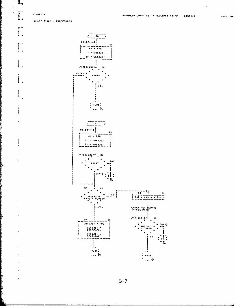
11/01/74 AUTOFLOW CHAPT SET FLOCHAT KTIfF LISTING PAGE 06
CHAlT TITLE - PROCEOUFES
/ 5,6 /
05.1 -----
I 01
I OX . 0j l I* . IE X - E E ( j J | )
I Ii EX * lEE(J.JI ) I
-----------
I
/KTI10490,. 0?
(-/.14.
.. AXOAY 0
I
1 (02
1 57
I 0 ---- - -
I I
I AY . aao
I I OY = Oo(JJI) I
I I
11 1 Ey - EE jIJ t) I
I I
I /KT01330/ 04
I I
• • (0)
----- ---- --- )
*----------------------A-- * LAO
• I
I(-/ ) .H'C FOP O
I I
1 65
I II II /KTIOI330/* 04
I Si6 I0
• - I ) I I 0I I ABS(AX -A
I EEa~ I .5 PP
I (-/4) * 'K7O Nr~
EXPL£ I .0I
I II VH J I 6I
I I
60! 6 I0
ABSIX -S-4 AA (A -AY-24A(JJ - 0.00.50p
L:.
5 * 3 *A4( l •**
59 1 0664
7.16: . I0
go 0 .21:
B-7

11/01/74 AUTOFLOW CHART SET - FLOCHAPT KTIPE LISTING PAGE 07
CHART TITLE - PRrCEOURES
6/ /
I I06.02"--)1t 07.32 --- 11
I I NOTE 14
4 01 * 4 * 04 * 4 CONTINUE 4
* (-/0)4 AF5(00) - *-+ I
s O*05*p. 1I* • I LIMIT PRESSURE IS NOT
4 4 I CONTQOLLING* ( •..*.. 1£
I * £ * /KTIO1700/i £5I **.. 4--..-----4; ...
I I
I 05*084--I
75 * 02 dO I NOTE 16
* * 4 CONTI1NUE 4* * ~TPUE 4 4 4* *
* AAO *EO. ARE 9-4* * I I
* 4 I STORE DATA FROM FRONT
*FALSE *7 FIE I
1 14 , !
I *... /KT13ta1o/I 17I 79S-- - - - - - - - -I 1 V9 = VV(JJI)II/KTI01f 0/I 03 I J? : UU(JJiI I
AMD = 440 - AAO I v VI I K9mIVOM (PPL -----------07.06*--) 4 Z9 UUK I
OF00/2 I 1 I 1 1I 1 08 N2 37 - NI I
I AAD = AMDeODO1M I I -------------- ----------------- I I
I 1 4 AAC *E. 4 TRUE II I (AAM 4 0.0011 4-. /KTI£1860/1 NOTE 10I I 4 4 K 4444*$4$*44
/KTIO1670/! 04 1 4 4 I dEGIN DO LOOP 4* 4I 4 4 I 4 10 N N2, 36
PALS * * 1 IFALSk **7"* - -- L 0 1-----------L0 I 6. --
4 4 £1 .*** I 19- -- I 80 1 S--- ----
* I ( 1 IN ) HH(3 -
[TRUE I /KTI01700/I 09 N1K I . . . . . . . . . I 2 OQON) ;,00(37 - II I I AAO AAO • AAD 4 I N)I I I ADD II I . . . . . . . . . I 1 EEE(N) - EE(37 -I I I I I N)
/KTI01670/I 05 1 1 1 1--------------------- * I £ I VVV(N) : VV(3? -
ADD : - 0.0? I I/XT101710/0 30 N)
---------- 4 I ALSE)lI FALSE * £
I I S-. AAO *LT. AAM 1 /KT10191O/I 204 06 1 ------- 2
4 24 4 I I UJU(NI UU(37 -I£SI4 4 I I N) I
4 •FALSE * £• 00 *GT. 0 #-. I ITRUE i I THETA(N) * 1
A I I I I THET(37 - N) I
SI ------------------
4 41 1 1 I4I III I
I TRUE I II /KTIO1710/I 11 I 110 4 21I •..4-............. I•I I AAO9:AAM4•0001 I • 4
I I I-------. 1 NO *I I I-. END OFDO
/KTI01680/I 07 I - ---- II i LOOP *S*------------2*
l ADD 9 0.0.1 i I• 12 4 •S.- --- 1... .. ..... 1 2 4
I I 4 YESI I 4 TRUE- 4AAO *GE. ARE 4 ---------
• * 78 1 134$ $ * $
I AAO - ARE I
IFALSE II
I /8.01
: 4.21.
4.21
B-8

110/4AUTOFLOW CHART SET -FLOCHAPT KTIRE LISTING PAGE
CHAOT TITLE -PROCEDURES
07*21;;1;/T07.2£---). NOE 1------- 08.110-1II
hh BEGIN 00 LOOP I ------ !X -------!1 NI2----------------
I III2 COMPUTE INPUTS FO A1(N) . 0 1PEAR SLIP LINE FIel-Dju;I I I 0. -- II I 0() *0 I I11 11
I I EO W N ) x 0 1 0 ; 0 1 - 0 0 5 7 3I I I IIII I VV(NI . 0 1 A P5.1 1 1 IA IP 5 . IwuI I UU(N) - 0 I I1 RO
I I I AOFXP(;!IS2.AD/ II I THET(N) -0 1 I1 1 S73I-------- I I II I I Z9/COS(AAO) FlE
112 * 03 -- -I
N END 00 00 I /KTIO235O,. 16~~~LOOP 4
e .I FALSE*I ---- PRO *GT. *RAMIN
I I I S
1 1 I
!KTt02020/t 04 1 II LOIF - AAO - AAM 1 I*------------------- T020I I f
I I I *---------------------- ~~~/KT102030/1 05I I I R RAI
/I I -------- --
PAIN 9I 1 18
1 I1 UUK-U9 - Z9 III IIKTIC2030/1 NOTE 06 1 I J I
I*5 I FF1 FOR/57.3 I* ADIF. OOO(N2). s I I 00=O
- 4 HH----------I -------I I
I I/1CT12410/I, 19:4C102050/3 071------------------ I---------I IFOT CCO *COBL--- -- NT----L I -------------------- I IfK-- 4 I ST102100/1 NOTE 10 1 1 AAU M AAM I
II* LIST ;G;0 * I AAI - ARSINIB11 I/KT102060/1 08 1 1 1I I I I TH2D;PI/2, I
/- IIII AAO +AA1 I/PA.INT 305 / I /KT102110/0 at I -----------
I 0 TRUE I /KT10245011 20II4 IGO.E.o 0 - .--------------------- 0II OUR z OUP(O.FF1I I
OPT FOR PLOTTING I PSI I- PRGRAMI .I CCO/TAN(FFI) II FALSE I II III SIG -PS/oUI IlK.T10IO1CzI 09 I I I I
/ EA FOM0E 1 1 1 EPO(FFEI T;Z.O) I1/ VIA FOR MATY /KT[02I20/I1 12/ 306 / I------- 4 I/ NT TE LIST ,' I13 1 H I
I1 1 PLOTSL N 1--/I to I. H-------- It 01 H 9.01
-----------
1 13
*8.34.
120
B-9

11/01/74AUTOFLOW C14ART SET - FLOCHAPT KTIRE LISTING PAGE 09
CHART TITLE - PROCEOURES
/ 130 /---------------------------- 0938-------08.20--- 11
1/KTI 02490/1 0 E I I 8----i
I I LREAR = L II OUA(ODIeFFZf I I
II 126 08 1I 0U3 I 1 * /KT102850/I 20
SlGIeOU2$cOSDOl) I 1I CC 1 * TRUE
/ /----------------- OF *LE. P A-. /I •
/ PRINT 99/I I * • I
//KTt02520O/ 02 •--------
FALSE 9 IT . XX 1 .•
/KT102850/ NOTE 21TRUEA • I•CO 130 ;*
* •
•-1 •£ 1
LIST : L. AA0. *I
OOOQ N2). HHH(NI./KTIO2620/I NOTE .09
,JAA,* $ * sA A A A *I jtFALSE 1 BEGIN DO LOOP 0 I
127N 1.31I1.36
/KTt3283/O, 22II I I
/ /I I I---------------I
/ PRINT 307 /CHECK FOR NO FAILURE I* / /CONDITIONS IN REAR I•I
I FALSE --- I----------------- I--. • O(N) *GE. •122 1 NOTE I II I PPL * * , s NOTE * I
/KT1O254O/* BEGI DO LOO
3 1
I T3 I I BEGIN 00 LOOP OPT FOR PLOTTINGI * IPRO RAM
I FALSE. ITRUE IIIII . .. O U 3 G E • ~. 0 1 1SI ------------- /KTt02890/ 231
I 15 II A I £ I ------------------- ~ IREAD FROM DE,0 -------------
I 1(IO I I/ 5 /I
II I VIA FORMATTRUE I/KTI02630/I 1I O0(N) - 0 I308I G------------ -~ I I
/INTO THE LIST/I EE(N) -
1 I O0 I-I I I A- - - - - - UU(N).0 I II /KT102890/t
NOTL 24
I KTIO2S40/I 04 II1 1 1 VV(N) = 0 1 A A A A A A A A A ,I ---------------------- 1 12 12 1 1 - - - -A I A LTIG AI X 3 A - ------AA A L ST IGOI • I A A NO I II I I.... 0Q•02A--II
*I END OF O0 A -A 1 124 A 16 I117 I 0S A LOOP A AA------------ /KTA020* 2OOF I I I A NO A A----------- A-
EOFO A-- -R~
• • • ND OF DO 4 . ..I YES LO PTUE *I ISI A LOOP A A...A IGO *EQ. 0 A
COMPUTE REAR SLIP A
ALINE FIELD I *,I
[YES I
I I I A I IAAI
IFALSE/KT02570/I 06 1 .1 IA-------------------- I 1 1I I H I9,9I
t 8 I SLFI H I I\1.1I H I• • * I /KT102?30'I 1?T I10 1 H I ... 130 ---- /KT02920II I I VVK - 0 ...A ................. .. .. . .. .. . I I I 1 H3A----------- I
1I I UUK - 0 I 12 1 PLOTSL HII t10
HI VVA - 0O0
III I I I IH/KT,02580/A 0T I I - HA -I I UATRUE I
I- I JJI - 0 I ------------ IAx AE TRE A- - ---- A I 111 12
XXX GEI 2 A -. I I I PPL A OOF I3A - - - - -A A 1 125 A 13 --A------- A 1 N3-N2 jiJ I
A A I A A I I I I3:N -JJA A I A A II1I A A TRUE I /KT270I I N4-_N2_- _,FALSE I A OP *LT, A -------- to - .I A (•9SAPPL) A AAM - AAM I
II A A I0
/KTIO2950/I NOTE 28I
AAAF O .AAA A--- I FALSE I AX x 0 EGIN OO*LOOP+ I 1 160 N = N3. N4 A- -- - GI
AI O * A** AAA**r I A.. ... .. . .. .. I III
II I 1/I I
9 .19. 4.19.... i30 . 52
B-1O

11/01/74 AUTOFLOW CHART SET - FLOCHART KTIFE LISTING PAGE 10
CHART TITLE - PROCEDU&ES
-----0Q.2------------- -------
I I 01 1 /KT103120/1 07 I- -------- ----------------- 1 190 0 13
I I HHH(N N) - HmN - I I I UI = UUUCN - 1) + I II I N3 + I) I I I (UUU(N) - UUU(N -I 4 •
U I I I 1 1 2 I0 NO
I I EEE(N) - - EE(N - I I I END OF 0 4-
1 I N3 + 1) H2 = (UUU(N - I LOOP • II I I I) - I I
I I O0(N) x ODIN - I I I UUU(N))/CVVV(N) - • 4 II I N34+1 1 1 1 VVV(N - 1)) I I *
I ---------------------. I I I IYES .10.I I I HI = ATANCH2) I I 1 06I I I . . . . . ..-- - - - - - - I I
1 /KT1029901i 02 I I, I .-------------------. I I I - ------
4 VVVCN) - VV(N - /KT103150/1 08 1 1 1 360 I 20I N3 + 1) + VVA -1......------- , /KTt03320/I I- - -
I X9 1A3 Ul - Z9 I I ---------------- I / /
I I I I I I I I RN. . 00VYI I I /I I UUUCN) * UUCN - A4 - VI - X9 I I I I I/ PRINT 365 /
I I N3 1 UUA I I I I TF = RCY2 I / /
I I Z9 I I AS SORT(A3**2 + I I I I/ /I I I I I A4**2) I I I OTT - OY8 I -
I I THETA(N) - Pt - I I I I I ---------- I I
I I THET(N - N3 + 11 1 1 1 U3 = 5*5(OOO(N) + I I I a I
ti I I.........------- 1 QO0(N - 1)) 1 1 I 1 /KT103810/1 NOTE 21
*I I -------------- S I I I * II I* * I1 0I I I 1 /KTI03350/* 15 1 LIST x BNF *
I I I 1I 1 * 1 •1 * II 160 4 03 1 /KT!03190/1 09 I ( 1I *• S -------....... I * ARSCIINF - C (-/0| I1
I I U .SS(EEE(N) + I I LO) - O.4L0 ----- /KTi33830/1 22I NO • N I I EEE(N - ) 1 1 -
+. ENDOF 00 1 I I / 1SLC3OP I I I US a (VVV(N) - I • /
I I VVV(N - 1))*2 1 1 PRINT 370 /SI I I I( /
SI I U6 = CUUU(N) - / /IYES 1 I UUUN - 1))S2 I 1 -
I I ------------ Ia . . .. I II I I I /KT133830/I NOTE 23I 1 /KTI03220/1 10 1 1 * I *I I I I
C I 1------ . , 294 16 LIST 8TF
U7 SORT(U5 I 4 S • • *• 4• •
•COMPUTE LOAO.ORAWBAR I I U6) I 1
AND TOROUE BY I I I I FALSE S I1NTEGRATING INTERPACE 1 1 Y4 = I I- - ------ LO *LT. RNF I /KTI33350/1 24
II U34COS(HI)3 5 • / /
T ISE I I U3*CU4S(N13 4 I I I 44-
/-03040/ 04 IY5 -1 / PRINT 375 U(U4COSH) - I I I ITF
V- 0 1 1 U3*SI4NCH)) I I I IIt I. . . . . . . . .I -- - - - - - - - --- - - - - - - -
I Y2 - 0 1 1 1I I I I
I Y3 - 0 /KTI03250/1 is I I I /KT133850/I NOTE 25I. . . . . . . . .I - - - - - - - - - /KT103360/1 17 0 1 * I I * •
I Yd - 0 1Y6 - I .. I S•------------------- LIST OTT
U7*U34(-A3*SIN I I I I APX I AP I 4444*4*45*4
I NTHREE z N3 I I (HI)+ I I I ----------------- I.................... A4eCOEINH)) I I I I I
I II ----- 31 1I Y7 I I I COR4UTE SINKAGE
/KT003090/1 UN1U4•(A3.COS(Nil I I 0 I II I I I I I S • • - A4•SIN(HI)) I I I
* GIN O LO 5 1 1 4 /KTto3880/I 26
• 190 N - NTHREE. 1 1 Y) z YI + Y4 I I * FALSE .-------------------.
36 * I I 1 LO LT. RNF - 1 SNK - UUU(N3) I0 4***4* I 1 Y2-Y2+Y5 I I I I
I -- -------- - - I i NSN - N3 IOt.13---it I ----- * ------
1 06 I 1 1................ . I /KT103290/I 12 1 TI'UE *it 0 II U2 0( N - I I- - I ------------------- 1 *. 17 /KT1339C0/I NOTE 27
S 1 I I Y3 - Y3 + Y6 I II .... 1* 4 1 1 * 1I 2*000(N)) I I I I I 4 SEGINOOLOOP *
I /(3•(G00(N) + 1I I Y8 = YS + Y? I 1 •30 N N3. 16 *
I 0OO(N - III) I I -------------------. 1 I 1 * I *
I I I I I /KTIO3370/! 19 I1 VI - VVVCN - 1) + I I ..................- 12.36 --- )II (VVV(N) - VVV(N -I I ----------- 1 AMX I - AAM I I
I ) *t)2 I I -------------- • 28*--------------------*
I 1 4 4 TRUE--------------- I UUUIN) GT. 4-e
S SNK * £/I1.17 * * £• • 1
IFALSE *11 .05.
385
*12.06.
... 380
B-11

11/01/74 AUTOFLOW CHART SET - FLOCHAPT KTIRE LISTING PAGE 11
CHART TITLE - PROCEDURES
10.18*--)*
S 1711.23*--}•( -- -- - -- -
296 1 NOTE 08 1 *s 88* * 0 *8 I FALSES *
• CONTINUE LO + . LO *GT. 6NF **8 ********* I • •
I I•* •I ITIUE
ADJUST PEAR AND I I ITFUESEPARATION ANGLE TO I I IMATCH LOAD I I I
I I I II I I I
I I -------------...../KT103510/! 09 1 1 /KTI03380/I 18 339 I 24
TFUE --I .---- --- I / /------------------------ LO *GI. UNF I I I I/ PRINT 340 /
298 1 01 - ----- )I I/ /• . . . . . . . . . * * I I /S B=1 I * ! I 19 1* * 1 • • I
I IFALSE I • II II FALSE • • II I I. . .- . L O G T . 8 N F • I
/KT103610/* 02 I • • I• •I I I* • S.21:
FALSE * / ,KT103520/IC I 1 1 ... 999..... ------------------ I TUEI
• * I I I II I9 I
ITRUE I IS/KTI3030/ 11 I I /KTI03390/I 20 II * •I I AMY -AAM II FALSC• * I ........ . -------------- *
------ LO LT. I I 1 1 349 I 25:KT103610/1 03 * •S*BNF •)
•I••I• I / /I 2FS / /
S........ ......... ••* / / PRINT 350 T)1 TUU
0 1 1* AP .EO. AAMI *12!---"--
I /I 26KT103530/ • •I I I -------- • IFALSE I
-1 1 5 ... .
I -- - -- - -
/KTI03640/I 05 1 13 E 1 1
* - - -- - - - - - - - - - -
•I AR I A - 4FB I /KTIC34101I 22FALSE * I * *
----- UE AI GT. MA • AAM -F(AAM I •It•I .07F ) I I•U TrUE
---- - - ------ --- AP EO. ARMIN I +..
• •0 I • $III * • I*
*- - -- - -I ------------------- - -
TRUEAI I F I1 /KT103560/* 14 • /KT103430/* 26
I 'FALSE I I
I I• • • I
I FAS 0• TRUEI :P ... • LT. AkMI. Is • ART ERD. 0 •-+
/KTIO36AO/1 06*•**
----------------- I-------*AMX *• "* * 26 • A *Y I
I ~~AR - AQMAX 1• •* *1---------- • /KTI03420/* 23 1
I0I TRUE I FALSE I- - 1 1 1 * * I 0I
30 07 1 TRUE I
I AY 0 I + AY-0 EI
I AX = 0 1 II I I
II AY - 0 1 /KT103560/1 15 1 /KT103440/1 27
I T : A H N IF A L S E II A R .5 0$ ( A R xI -- - -----.. .. .. . I I ARY) I
I I I I-- - - - - - )I I i I AAM .5* 04ANX + I
.20*12.01. - - - I A 1.1• •i AX 0 -- - - - - - - I AX - 0 1
3 0000 1 1 1I A!: 0 1 AY - 0
I1I I
.12.01: .12.o1.;0.* 0o ;00. o
B-12

11/01/74 AUTOFLOW CHART SET - FLOCHAFT KTIAE LISTING PAGE 12
CHART TITLE - PROCEDUALS
300 f / 385 /
llo07e-- I 10,28- -)--... ........ .....--I 01 I 0S 1 /KTI34080I NOTE 14
- - --------------- ---------- . I---I ITEP = ITEQ + I I I SNK = UUU(N) I I dEGIN DO LOOP•---I I I 1 444 N N3. 36
I I NSN - N I 1 0 S S • * * S S
I I I ------------- I/KT103690/ 02 10.28--- )I I IS
- * 380 5 06 I /• TRUE I I / /
STEQ.rE. 20 - - -------- )S • • / PRINT 433 /• 5 329 I 04 * HO / /-- -- -- -- -- END OF 00 1 1
• •//• LOOP I I|- - - -- - - -
- FALSE PAINT 330 / * S I I/ / ; eli. KT134090/1 NOTE 16
I / YES 10 . I It ••----- - 1 28 1 1 LIST :N, HHH(N).a I •*• •JJO(N). EEE(N) .
/KTI03700/0 03 ... I I I5.1 't •/T103960/1 -------
/TRUE I SN/N_12*SNK I 1444 17XXX EO. 2 ;99 ----- - ----
I I I NI /KT103970/I 0 I T..0.-- END OF 00
--LIST ------- LOOPFALSE ,ee
51 * 4 S 55 5 5 5 /
/ t/
P I I YESIT 30! / /
I II
I KT/03970/1 NOTF 09194.18• * * * IC * I KT[04120/1 18
- LIS, - - -N I -----T-RUT -
i I PRINT 309
COPUTE INPUTS FOP I PPAICLE PATH I ---GEOSVMETARY I IIII I I
I I /KTI34120/1 NOTE 19IKTI04000/1 tc I * • • . * * *- ------------- * 1 llST*: RUTO. :I UTD UUUIN3) I I X01S.*Xppojo :
I xOIS -VVV(NSN) I I
I I II XPP0J -VVVIN3) I I/KT13A1A011 20
iI / /
I I PRINT 402 1COMPUTE PULL AND I/ /TOROUF COEFFICIENTS I /
I II I I
/KTIOAO0/i II I
I PUN S OTF/PNF I I FOR THE COMPUTATION
I I OF INERTIA FORCESI TON I I I
I BTT,,i2%NF) I I I-------------------- - I /KTI04170/1 21
I II I READ FROM 0EV -
/KTIGS060/1 12 1 5 /-----------.---- / VIA FORMAT /
/ / I 400 // / I / INT0OTHE LIST /
/ 9PINT 39 / I/ / I
/ / 1
1 /KTI04170/I NOTE 22I I * * * 0 * S 0*I I LIST =:VEL, ZOEPt
/KTIO060/I NOTE 13 1 55*•* *4**
SLIST PUN.*TON 5 1
I I £ /-' ~II
----------- 13.01
B-13

K /O1/74 AUTOFLOW CHART SET - FLOCHA- KTIPF .ISTING PAGE 13
CHAOT TITLE - PROCEOURES
/ 420 /
12.22--- IsI I
/KTI04190fo Ot It ...... 1 /KT10452011 19•KI4R/ 0• --------- - -AI A15 I I SSLIP SSL/CNO I
TRUE I ATAN((ZA (NI - K . . .VEL I II/(XA(N| - I I
• • I I XAIN 4 1I)| 1 /KT104530/I 20
* S I----------------------------- SI F E I I / /IFALSE 1 - -. .... .. )I / /! , 1 430 I 12 / PRINT 460/I
I*I I AKI - COS(ANA -
I I A15l -- -- - -- -- -I 9
I/
AKS K I1/KTK04Z00/ NOTE 02
TAN(THETA(N)) I I /KTIO4530/I NOTE 21BEGIN 00 LOOP I AK2 *4LISTLRONT,0 410 N N3.•36 : AKF.IO(AT)SAKSSINCA5)
LREAR. SSLtPI I I COSCAIS) K • •e...$.. s
-------- II Ag3 II I.. ...... 3 AK3 - I
. . .03 I VEL/(AKI•AK21 I /KT134550/1 22--- --- --- --
THETA(NI ........... / ........S*5s0 - THETA(N|IX V ( I-- /KT104430/1 13 / PRINT 465 /I X9 1 -------------------- - / /1I
I A16-1.0- I / /I ZAIN) * UUU(N) - IAK; AK21 I ................K II
II - - - -- - -- - IK IASSU4E ZETA FORi
/KTIOa4O! 14 I PARTICLE PATH(AS 0.9410 * 04 I IF NO OATAIK a
K S $ TRUE KNo • I N eEO. 36 ----- /KTIO450/1 24• ...... END oOF O00••", .*,;;-;;;;L- EOOFO E I IS K I /AFRO OEV• LO * I• • K / 5 /
I/ VIA FORMATIFALSE / 470 /
IEsI / INTO THE LIST /II [ ... ..I. .. ..I I
I /KTi04580/I NOTE 24I
/KTIO&45C/I 15 * $ , , 5 4 $ ,ITO2I I •-- - - - - K LIST ZETA/KT104260/1 05 I--I--R---I---S* *S~~--------- CHORD I I s•II C HO - 0 1SORT((XA(N) -I I XA(N - 1)1**2 I I IK I I I I (ZA(N) - ZA(N - I III I I !) 2 I ICOMPUTE RHO FOPI IHOK K0I I I PARTICLE PATH FROMI CHOSL I I I I CHOSL - A16CHOPO II SLIPI------------
II( ,.SL.SSL4CHOSLK I I,/KTII4290/K 06
I /KT134610/I 25/KT0490I 6 K I K I ----------------
SI I/KTI04480/ 16 , ZKSO - ZETAK I2 IS/ I I -- - -S K II LIC.ET,./ PINT 415 / CHI + CHOO ZKCU - ZETA3/ I I -- 1 ZKFO - ZETAS** I..
I I I ---------------II...---------- - II 440 1 17 i
KX1430l I7 1 ------ --------------S K 01460I2/KT104310/l 07 K • .- 1 K0------2
*---------------I---- - - - - -1- 1 4 0 =- 1K N.•36 I Il I 1.401144ZKSO + I
------ )0--- I K K I 2 372180ZETA. II I K K I 1 I 2.01924 1I 1 /KT104350/o 09 1 /KTI04510/ 18 KI I A ICOMPUTE VELOCTY 1 " 1 . * 1 ABI-- ISOUNDARY CONDITIONS I • 6I TRUE • 315 TRUE I 1.05039*ZETA +AND AVERAGE CONTACT I * N *LT. 36 .... K S N 0G50 Z-.SLID I N GE N3I 2.0157SID I * * * • K I --------------------
13.16 --- l I417 I 08 eIKT10466O/27*------------------ IFALSE IFALSE.'3. 0--------------
I RAO • I II 1 . 0 . 1 1 482. 1 -I SORT(ZA(N)0$2 + 1 K I **** I 10.9S6SZKCU 4 1K XA(N)002) I I I 417 1 1 24.68440ZKSO -I K II
I I I 17.6294$ZETA +I TN 414.I IZ(N I I 1 1 1 1 4710ATANXA(N)/ZA(N) I I/KTIO4360/i 10 4.................... I ------- 601--*-------------- ------ ----------- -------------------
I•*--------------- ------
I II1/
------------------ /14.01
B-14

4 AUTOFLOW CHADT SFT - FLOCHAPT KTIFE LISTINf. PAGE 14
CHAPT TITLE - PRnCEOUAES
/ 484 /
13.27---)- - . ...------------------ ----------------------------------- I-I/KT104670/. 01 472 - 09 I I 1 22
- 4-- --- 4 ----------------I A 3 1I OFNO = I / /
I 717.661ZKFO + I I .S*ZETAOSIO(RHOO I I /1!250405 CU I I 1 ZETA.OMTEN) 2 / PRINT 480 /
I 3253 00ZKSO I I I /COC(RHOTEN I / /1 1863.36.Z TA - 4 . / /
1 396.737 I !
ZETA I I96.737 1 1 1 - - - - - - - -
I /KTI04860/* 10 /KTI35010/I NOTE 23/KTI046QO/I 02 I • • 4 * 4 4 4 4 4 S 4 44 - ; .- ------- I * 1• LIST OEOI RHO I IARSCOENO - 4 TRUE I I NE1. ONE2. OE3. *I AR14(SSLIP::3I + I 1 * 1.0) *LT. 1.0 ------------------ Is I ONE 4I AC2 ISSLIP 42 + I 1 4 I 2 I * 4 4 4 * * * SI ARSSLIPAO I + A D ------------------- * I•----------------- I OME4 * OMTEN I Ii
1 I /KTIO5030/1 24I I IFALSE I I = LFPCNT/VEL
/KT104700/1 03 2 I 1 1 NI I I I TIM3 . TIM + / /
/ / XOIS/VEL I I / PPINT 481 // / I/ /-- / PPINT 100 / 1 1 1 TIM = TIM3 I / /
/I I I I (XPPOJ - XOIS + I---------------/ / /KTI04870/ I I LRrAPI/VEL I
--------- I --- -- 1 ------ * II * I /KTIO5030/I NOTE 25i I FALSE 4 4 II I 4•• 4• ••
/KTIO4700/I NOTE 04 2 .-. ENO *LT. 1.0 • /KTI0499c/I 19 1 LIST 6 TINI.......... * 4 .... I * ---------------- £ TIM3, TIM4• LI T4 ZETA, 2 • *• AZERO : I 1•444 •44 •4•*•4* SSLIP: PHO 1 I I I PUTO/(COFIPHZ. I I I
* * * * 4 * * * I I I I OCNEo - I II I I ITPUE I I COE(PHZ.OMFAI) I II I I I -.........------- 4 I /KTIOSOSO/o 26
/KTI04720/I 05 2 I * *I I I
---- ---- ---- TRUEI I4I H79RNO*0TETA I • ........ TRUEI I I I I 4XX *EO. 2.0 4-4
2 rSAR = I I /KTIO4870/I 12 1 1 1I ATANI.S4ZETA/TA I I I -------- 4I I.24PI - I I I I 003 - ONTEN I I 4 1
I SOFFII I I---2---------- -I- ---------- I I I I FALSE *126
I ------------ II 03I I! I * *
I 1 1 3 I I 482COMPUTE OMEGA I 4 2PARAMETER ANO TIME I 4 IVALUES FOR PARTICLE I FALSE 0 1 /KT135060/1 27PATH I .----- DEND .GT. 1.0 1 I ..................
I I 1 41 CKl - OMEVE/PlI2 • •/KT!04750/0 I 1 4 1 RAT4 I
S ------- 4 1 1 1 TAN((OME3 - II OME I I I [TRUE I I . *0 MEVE)/CKI) I
I 2$FSTAR/(t 14I III I I I 2 I RATI II OUFI PI/(i4 I I I I I TAN((OMEO - II PHOeZETA) I I I I *SOMEVEI/CKI I
2 P / 2 I I 2 * -- - - - - - - - -OF2 I 2IPt/(l + /KT104880/1 14 I I2 H ) I E I . . -------- I I
I I I OEVE OTEN II /KTIO5090/1 28O E 3 - 3*P / (I + I I 1 ..--- ---------- ----- -- I . . .. . . .. .
I QHOOZETA) 1 I I I I PAT2 I-------------- ------------- 2 I RAT4/RITI - 1.0 II I I IS25
-•--.....----- I I T140 - TIN3/RAT2 I/KTIO4790/I 07 II IUIT - IOUIT + I II I
S------- 1 ----------- I CK2 II OMEVE, I I I I RAT4/(TIN3 +2 2*Pt/(RHO - 1 I - T-------------- TIMO)I I I /KT104900/I 28 I I I II OMTEN I ........... . I 2 /KTI04920/4 20 OMCI II . (OMEVE + 031 / / • I 1 * I CKteATAN(CK2* I12 I/ / I• 4 TIl40I .54OM!VEI OEVE -OMEVE I I/ PINT 476 1 I 4 TRUE .......
/ / I 1 OUIT .GT. 20 4-4I TIO 0 1/ / 1 1 II I I - - ----- I I I /KT135130/I 29I 003 03 2 I 1 1 1 ------- ---
............ I...... I UI MC3 III /KTIO4900/I NOTE I I IFALSE *IS * I CKL4ATAN(CK2 II 4 • 4 4 4 4 4 • 4 4 • i * 22 * I (713 + TIMO)) + I
* ,/KTI04840/I 08 2 4 LIST * UMTEN 2 1 I *. 1 .. OMEVE I4-------4 0 I 4 • ••N•O • I 1 1 99I I4 1 21
I I I I I /KTI04930/I 21 II I --------------- I *.........------- 2 /--------------. I MTEN = .54(003 + I
I I CEVEI I /t5.01
------------
B-15

1I/01/74 AUTOFLOw CHART SET - FLOCHAPT KTIPF LISTINC, PAGE 15
CHART TITLE - PRRCEOUPES
14.29---)*/KTI05140/i 01
/ /
/ PRINT 488 // /
/ /
I
/KTIOSI40/I NOTE 02*4* 0** *e*0* LIST - A7ERO.
TIM0. TIM3. TIMP. *
* OmCI. OMC3
14.26---)!
482 1 NOTE 03
* CONTINUE s
COMPUTE COSTANTS INOMEGA-TIME RELATION
I
/KTI05IO0/I 04
I CKI x OMEVE/Pl II I
ITA = TANC(OMEA - II *S*CMEVEI/CKI) II II PTI - TAN((OMEI - II *SSCMEVE)/CKI) I-------------
I
/KTi05210/I 05
I T2 * ATA/ATI - I1 1.0 1
I II TIMO TIM&/RT2 II II C92 - RT4/(TIM3 + II TIMO) II II OMCI II CKISATAN(CK2S II TIAO) + .SOMEVE I* ----------
II
/KTI05250/I 06
0 -- --------I OMC3- I
CI*ATAN(CK2S II (TIM3 + TIMO| II *5*OMEVE II II AZERO II PUTO/(COE(PH? II OMEII IICOE(PHZ.*0MEA)|
/KTI052TO/t OT---------- S
I /KIOS5280/100/ /
/ /
/ PINT 48* / . ..--------------------/ / I/KTI0S2S0/I 09
// -------------------------- I AI I AX-C
I I II I I AY - 0 1
/KTIOS2T011 NOTE 08 1 1* * SA* S* I I ARX 0 1
* LIST * AFERO*. I I* TIMO. TIM3. TIMR, * I I AMX - 0 1* OMCI, 0MC3 1 I
* ** 5 AS 95 11 APY - 0I I!
I I AMY 0 1--------- -----------
RECOMPUTE gSLIP LINEFIELDS FOR INERTIAFORCES
I1 10
B-16

11/01/74 AUTOFLOW CHAPT SET - FLOCHAPT KTIPE LISTING PAGE
CHAPT TITLE - SUqPOUTINE SLFI
/ 1300 /
I05.100--I ------------ I ----------------- ----------- 8.-
I NOTE 01 1 1 /SLF00590/I 15 1 20 1 23* 4 * 4 ** 09 I ------------- S ------------- S
0 REGINOOLOOP I s " LIc I I I INTP - 0 I3 I = 1. 49 1 0 I DIS(A0.ATT2.TI. I I------- - ---. .I 0 4 0 * NO I F I I
I * END OF 0 - 1 1 1I ------------- I LOOP I DAX. I I /SF00690/..I 24I NOTE 02 I 1 1 I ATAN(SIN(FI-I-
• REGIN.0OLCOP * FAC-2 I I /* 171 0 0 I I YES I *SSOIOIiDAX I I/ PRINT 19 /
I./ /I I *I...* 1 1 /.--------------II I I I itI
I 03 1 1 1 /SLF00620/I 16 I I------------- 5 1 I 1 I - --- -- S; II •SF06/ 10I
i X .J) * I /SLFO36O/I 10 I I L2 II /SF0690/I NOTE 25I- -...............- I FACLISCOS(UI) I * . . * * * * *
I ?(I.J) - 0 I 1 1 z49 1 1 I *COS(T3 - I I LISTI I I I I I I FII/COS(FII I 1 4 LIST•*w * 4 •
I S(I.Ji 0 I N 17 1 1 - ------------------- II I I I I I I I... T(I.J 0 1 1 1 INTP-0 I O I I
------- S I I I I I I I SET dOUNDARYI I I1 I = 3.14159 I 1 ESTIMATE L DISTANCE I CONJITIONS AT FREEI I 1 1 I FOR PASSIVE ZONE I SURFACE
SI I I I GG - 32.2 I I I 1 1S 0 I I I I I I
• I T. - TANIFI) I I /SLF00640/I 17 I /SLF00720/I NOTE 26
S I I ----- 7------ L L--- --- I*lI*DlLO c* I NO. -. . I " dFGNDOLOOp oC
EN OF FNI O S I I --------------------------44 I x 1J . N* LOOP I ISLFO04Z011 II ! 5 4 4SI I !S--20------ 1
4 1 I I AF * TANIDI) I I 19.09---ItI I I 1 I /SLFO06S0/ 18 1 27
IYES I I 11 2N - I I 1 0 ..........-I I I I I I I IzN4I-J I
I CI CO/TF I I * TPUI II 1 I I S VEL .EO.0 4---. AJ J I
i UI I P-/4 - FI/2 I I A I I* I * 0 AN - N II I I F3 - I - SIN(FI) I I * I
3 0 1 I ------------- 1 Z(I.J) -0* S 1 1 I I FALSEII
I I X(.J) (AJ- I5 5 NO I I /SLF0040/ 12 I 2L/|AN - 2) 1END OF0 ... ------- I I I -------------
• LOOP I I 3 - -- TAN(FI) I I IIS •II I
S .I I V- I I I /. 1OT80/I 284 I I I I /SLF00660/1 19 I...... .EYES I I VS - TAN(FI) I I t I X(N.1) * 0 1I I I I I• I II 1 V6 1 I I FALSE * I I A(N - 1.2) * III I I ... XX *EO. - 1.0 5 I *SSL/EAN - 2) 1I I I 020 I I * ...........---------I I ------------- I
/SLF00250/I NOTE 00 I I S I I
8EGIN 0O LOOP I /SLFO0520/I 13 I I ITPUE /SLF)0800/O 296J-1.36 1 -- ------- I I I S ,1 I 03 ELL(D2.Fi I I I I S SI I I I I I TRUE
IR.09---II I I TI - (03 - 02)/2 I I I I *VEL *E. 0 *-•I 07 I I , 1------------------- * I I OS - 010(1 + I I I /SLF00660/i 20 1 * 1
A(J) - 0 1 1 OF)I/2 I I I ---------- 5 1 * 1I I I I I I L LFCNT I I *
R(JI * 0 1 I04 1 OEL(OS.FIJ I I I ------------------- IFALSE * 19.- 0 I ------- * I I I 1 07.
ClJI 0 I I ------------ I! It 12I! I 22O(J) - 0 1 1 /SLF00560/I 14 1 21 1
II/ + - - - - I 1 S II U(JI - 0 I I T2PI/2 I• II I 1 .54(04 Oil - I I FALSE I COMUTE INERTIAL
V(J) -- I I I AO At I * XX *EO. 1.0 0 ----- * ACCELERATIONS AT FREE----------- I I I I A SURFACE
I I I : C1 I I II 8 I 3 75P I 1/L00320/ 08 1 T3 *75P+ I I I /LF00820/I 30
--------- 5 I 1IF1 - T2 I TI I I ITrUE I * ---------------S H(J) 0 I I Ao AI I I I 1 12 1 HI I I ------------ I I 181 ACCE 1I O(J) 0 I 1 1 I I II HI I I I101 HI E(J) - 0 1 I --------- I I I H------ I. eSLF00670/1 22 I* --------------
S----------I- I L EA I II II
-........... . 19.01
B-17

AUTOFLOW CHAPT SET - FLOCHAFT KTIFF LISTING PAGE 19
CHAPT TITLE - SUSPOUTINL SLFf
18.31---)* -- */SLF00830/i 01 1-- • 40 * 09
I 02 = * 0I ATAN(ACCX(i.J) I £ •I /IACC7(I.J) + I * NO
I GG)) I • END OFDO -------------------- LOOP • I
I I$a a I
)I IY S ." '
/SLF008401/ 02 IYES• * I I *27.
* 4 I l t
FALSE • $ iS..... *8A5(02) *GF.* I1 *A8S(.99 rI) $ Ic I /SLFO0950/I IC
I S --------------------TPU I NET w 2*N - I i
II II tI II I COMPUTE SIGMA AND
I I THETA AT SINGULARI /SLF004B0/I 03 I POINT
I S-- -------I 02: I II .OQ4FI*O2/A8S(D2I I 50 I NOTE 11I $------------------- * *5*54* 0 *4
I I PEGINOOLOOP 0-I-- - - - 70 I N. NFT
I •$Ae$$•I04
- • IIITRUE • S ..... .... .... ...
•4 1 AI FLOAT(I)I AN = FLOAT(N)
I IFALSE II II
I I(IiJI 0I I I I I (I.Jl 0
---------------II I
I /SLF00860/I 05 1 1 I-----------------I I /SLF01030/I 13
S / /------------
I / 1 I TI (J) ATI / PPINT 350 / II 2 - TIIIA! -
/ / IAN)/(AN- 1)I / / I I II
I--------------------------I I I POW. I
SI EPO(FI.T(I.J).TI) III I
/SLF00E60/I NOTE 06 I I I S(I.JI - I1 . . . 0 5 0 4 * • 0 * I I I POw6S(Ni) II LIST J. 02 ----I--------
I e5 e. 5e e ** * I IIII I
*--... 294--It I l
22 I 7 I 70 4 14------------------- I1 03 OFL(D2.FII I I 1I I t NO •I T (03 - 02)/2 1 I.. END OF 00I 1 I LOOP *
1 W2 0 OUP(O2.FII I I
I I I. 4I * ul/? I I
I I I IVIESS(I.JI SI I I
------------ * II I II I!
/SLF00930/I 08 I------ ------- /SLFOt070/I
I TI.jIJ TI I I- ----------------------- I I 02 OUA(0I.FI I
I I * Ii) = O e I i
I 1 10(1) *0255(2*N-- - I I.i)*COS(0ll - CI III
i E1) : (O(I) + I
I CIISOAF I
I,
WIJ~) = 57.3eA0
/20.01
B-18

I
.AUTOFO CHART SET FLOCHAPT KYIE LISTING PAGE 20
CHART TITLE - SUBROUTINE SLFI
59.55---'.
StFGSiSIO/I 01
I THET(I) S T(2$N - I
SIL I
I
/SLF01SO/1 NOTE 021
* IF0129IAU200 j 2.O N-----ES 0 [ OTE 1 I U02 I
I I I 2TF*IS(I.J - I- 22.07---) I 1 I T(i.J - I I
1 03 I 1 S(1 - 1.JlIT(I I0----- I I .J)) I
I~~~ ~ !.J) I --------------------I JS I
KNT N *2 - J 22.05---)iINI i 85 10
I JNT S 4 * 25tN - 5 .. .... ... .... ..
1S I I) VI = TANITHI) I
I II V2 * TAN(TH2) I26.120--)l I I
80 I NOTE 04 I I XI - VISXII.J -! 5 * . * 55 . 1 1 1)8EGIN 00 LOOP S I I I
*190 I KNT, ..DT 4 II xj V2sX(I - I**•********• * I S IJ) I
I I *--------------------22.0b---) 1 i
I I I* 05 I /SLF0I340/i it
1 I-- ---------0 I I V12 a I/(Vl - V2) I
* 4 TRUEI I I* I .E . (J * *- I XI.J) S
1)2*(N - 1) 4 I 1 VI 2*Z(I - .iJ) -I I Z(I.J -XI) +XI -I
I I IL)
* .. II IFALSE * 22 * I Z(iJ) =Z(I SI * I I S lJ)J))(X(IJI II *. II xCI - S.4)iiV2I 126 I . .. . .. ... ... .I I II I I
1 SLF¢I20C/I 06 I
----------------- I /SLFOI3?0/0 12
K - 0 I I *
THIIIJ- II 4 TRUE1 17 • US I I 4 VEL *E0. 0 ---------
I• 4 86 £ 15
I TH2 - T(:- * S .I .1J) - U I * GH 0.0 1
sli S(I.J - ) IFALSE I GV 2 1.0 1------------- 4 1 - - ----
I I/SLFOI240/I 07 1 1
-- - - - - - - -. ..-- - - ; II 1 SI S41 - 5.3 l II 2I I COMPUTE INERTIAL .21.01.
I V7 * 2'S(I - I I ACCELERATIONS FCM *1I .JIS(liJ - 1) 1 1 PAPTICLE PATH ... 8
I I I II U9 S(i - .J) f I I I
S(I.J - II /SLFOS30/I 13
I 512 I H1 18 1 ACCE H
/SLF01270/I 08 1 1. I H.. . . . . . . . . 1 102 HIV8*•(T(S.J - I 5 1 H
115 - TII - I ........ --I .JiISTF I II
I V?9 2;Sll - I --------, I-I )*V8 I II OH :ACCX(i.J)./GG I
I I GV - 1.0 I IS I ACCZ(I.JI/GG I
-------- *---------I
. II
:21.01:
as
B-19

11/01,74 AUTOFLOW CHART SET - FLOCPAPT KTIPE LISTING PAGE 21
CHART TITLE - SUBROUTINE SLFI
/ 68 /
20.14 4--)!--------- *
V3 •GH --GV*TF II
I V4 GV + GH*TF II II VS - GH + GVOTF 9I II V6 - GV - GH*TF I--------------------
I
/SLFOI00,i 02
IA * V3*IX(I.tJ -I X(I - I.Jl) + II V40(7(I.J) -I (1 - I.J))II Pp w V5*(X(I*J) - II X(I.J - 1)) .I V60I(Z IJI -I Z(I.J - I) I
.SLF01S20/1 03--------------
I US SII.J - II - iI S(I - I.JI I-----------
I
/SLF0530/1 044 *
4* 4 TRUE* U9 *LE. 0 - .... . .
1 £10 1 05
rFALSE / PRINT 112
I I
:22.01: .26.14.
115 ... 250
B-20

31/01/74 AUTOFLOW CHART SET - FLDCI.APT KTIKE LISTING PAGE 22
CHART TITLE - SURQOUTINE SLFII! K
21, 4- -) 2 ,0 ----- --I
- 1
I T(K J) (V # I I
U6 + GO4 * - IAA))/(2*TF*Ul| /
1 TRUE *
/SLFOi600 02 ... XX *GE. 1.0 0
* 4 TAUE1*SK EO. K ---------- 22.02*--)* KFALSE
4 * • 190 4 06 K
IFALSE * * NO II ENO OF O0 *.
LOOP 4 K /SLFO7--/ - 1-
t * 4 I I X9 - XO iK *YE .'.0. 1 K
/SLFO0I0/! 03 [YES 20 Z9 = Z0
1- - - -5 .05. - -- --- -iK .THI * *5*(T(K.J - I I .... KI K) TII*J ) * UK K 1 )I
II K 125 K 15I TH2 .*5(T(I I I------K 1.J) T(.4l)) - I I I t X(J 4 2*N £
UK K 200 * 07 K 3.J -K)- XO KI si Z4 + " +KSII * ,S(ISI.J - £ 4 I 62 - Z0 4 2(4 4 K
K 1) + S(K.J2) K * * *O I 2*N - 3.4 - K- -.---------------------- END OO *-* OF --- * *
I LOOP !!
/SL . ..6401 .0 /SLF.)180/ 1
51 1 .5 ( 1 IYES *201 :, S(* ) 03*•
.... TAUE 0U6 --- 10*X ED. 1.0
I 2*TFo(S KT(I.JI it ) S!2*T(I - 1 24.13*--)1 * *I*J ) 2 2 0 I 0 -*8
V7 . Sit1S(I - OF = Wl(l) I FALSE1.4) 1 1 *SK?*SKIJ - K) I AP N IJI) I K
vS(P016?O/I 05 I /SLFO1790t/ K?------- --- - /SLFO280/0 09 * ..-. . -
S I V9 2*SII*SI2*VS I 5 4 K GA ATA ---/-2 -K
g SKi. SK2 K X C 10 TI U9 K 1 I 4 X * TRUE l
2 - -- *G- -. ---------- 2 o III K K 5 4 230 I 1I I----- ---.--------- -; ------ I /SLgOIdOO0s toI * K VA*•xo K I *
I S A K K I J
SIFALSE I UA - 70 1 K1 + 20(N - 0 TRUEI ----------------- 1).J - *-
SI I K.LT. (UK 0
:20.10. K K 6 10) * K
OSI I ... K
/SLF0290/ I o• FALSE • 24...------------------ .26.15. K * 04
K K9 - 0 1 I KI I ... '000 I K 151I I I2IK VK - X9 K ---- K-NOTE-19I I,13 1 N .p OTE .19
Z9 1• * • * 0
I VA CONTINUE *
I Uv"0 I 0
COMPJTE COORDINATES1AND STRESSES AT
KINTERFACE* .
.26.15. 1
... 1000 I /
/23.01
B-21

1/01/7?4 AUTOFLOW CHART SET - FLOChAPT KTIPF LISTING PAGE 23
CHART TITLE - SUBROUTINE SLFI
22.20---)0............-1t/SLFOA30/! l 01 1 1S-- ----- 1 /SLF01920/* 09I A(J) = 1 2 •£ ATAN(61/G?3 - Al I 1- - - -- -- FALSE
1 I C7 .GT. A() . -
I I/SLc0P140/9 02 1 I
* 9I * IU
• XX .EO. 2.0 9-U 2
I I /SLFC1920/I 10 IIFALSE ------ -------------. aI I I I A ( J- -7 I I
I - ----------- M------------
I I 137 1 it
/SLFOISSO/. 03I I n*011 I* . I (I - OF) (A(J) II I A(2))I(AM - ITRUE 9 1 1 A(2)1) I---- xx GE. 1.30 • I II I OAJ = TAN(D(J)) I1 1 1
9 . I I 81 OEL(O(J).FI) I- --------
' A L S E I II I Ii ISLFCIQ6O/I 12
I I I 82 - 5*5(9(J) + I22. 1---)I I 13 1
132 1 04 I ---- --------------- I
I K7 = I I l~-----------------------I I SET THFTA AT ----)-- ----- It I INTERFACF I /SLF0200/1 16
136 I 05 I I ...................... ..... .. ... .. I X(I.J)~ 3I5 9 - VK + - I I /$LFC1980/ 13 1 1 Z3*(X(2 - l.J) + II X(J + 20N - 3.J I 1 ..------ I Z29X(1 - 1.J -1) T(I.- 204N - I I 1) 74)I 1 2 I) 23 P2/2 • 82 I-I G6 : UK + Z0 - 1 2 I A(J) I I 11Z(1.J 7(I II Z(i 2N - 3J - 1 1 1 I.J - I1 13 1 I TH3 .50IT(I.I I I I TAJ*(X(I - I.J II I I 20(N - 13 1 1 - X(I.J)) II 7 = I T(I .1 1 - - -.......I.......
ATAN(G6/GS) I I 20(N - ) I I--------- 0 1 ------------- I I1 1 I I I! I 1 1 /SLF02090/0 17I I /SLF02000/I 14 I */SLOIQOO/9 06 2 .. .....---- * IT-"T
* 9 I I 1 9 VEL EO. 0 -------------------------FAL SE * 1 1 THS .TANWTH 4) I I.... I E0. I I I I I ! - i - -- !0I 9 TAJ x TAN(A(J)) I I 9 9 1 GN 0 A•I I I III: 0IZI = I/TH5 I I IFALSE I GV .0I9I I I I I*- - - - -ITAUE I I Z2 - ZI*TAJ I I I
.I ------------ II I II 2 12o3 ,I I /SLF02050/! i5 I II I *--------------------* I COMPUTE INERTIAL :24.01.S/SLF01900/I 07 1 1 Z3 1/(l + Z2) I I ACCELERATIONSI .---- - -- - I 1 1 1 ... 44I A(J - G7 1 1 Z4 - 711(Z(i1 I
I -- ----- I .J - 1) - Z(I I I /SLFO21O,/I toI I I l.j2) I 1 -- - - ---------- )I 1 -------- 12 1 H
I 08 1 1 18 I ACCE H•------------ I. I HI Z. • II-- - 20 H9-- --- 9 111 1 H
I !
/SLF02120 1 19
I Gs cc AC(IJ/G II I---------I OH*ACCIJGG I
III
I
.24.01.
1 44
B-22

C11/O1T4 AUTOFLOW CHART SET - FLOCHART KTIRE LISTING PAGE 24
S CHART TITLE - URlROUTINE SLFI
1./ 244
23.19e--)1!
! Ol
1 V3 - GH - GVOTF
I V4 x GV f GHOTF II AA V3(X(iJI - I
£ LIZ - 1J)l II I)
/SLF022IO/ 02 I* -( I 1 3 0 11
* K U3 * 205(I - 13 • 1
S I.J)I*TF (T(I J I I * 4I T(! - I.Jl I I TRUEI I I CH3 *GT. *-t S(.J) S(I - I (AM + *C35) II 2.J + U3 + GIOAA 1Iz I
1 0: OU&(D(J).F F .'*------------------*K IALSE *.
COMPUTE NORMAL ANDSHFAR STRESSES ATINTERFACE
I I /SLF02400/* 12I K
/sLO022SOl! 03 1------ - ----- TRUE
1 00) 0 CH3 *LT. AN - ----------I Ole$(lJil • 1K *COS(O(J)) - Cl O 150 • 16KE(JI (0(J) K • • S
K C1)$DAJ I K FALSE $ • TRUEK K) :2 J J *LE. 9 0-.I VIA2 X(J LE 9I ?*(N - K).J) I •IK
• 1*--------------------S
I FALSE * 26
/SLF02280/! 04 /SLF02420/! 13 K • 07
U(JI Z(J I • $ K 165K ?SK - .J) K • * TRUE IK XX *GE. 2 $-5 KI THET(J) - T(J I • 5 K KK 20(N - 1).J) K /SLP32480/ 17
IG3 7X(J 2 lN $ * • sK I - X0 FALSE • 22. • TRUE------------------- 1 08 INTP EO. 2 -
I K2 I 5 K/SLRO23O/ 05 • •
64 * - 0 , 1lJ 4 K •KFALSE .*2'5
20(N - 22.J) K CHECK FOI MATCH 0F K * 06K K K NORMAL STRESSES I
CH3 - ATAN(,G/r4 l 2 I £55
K H(J) - 57.30CH3 I I i------------------ K 1SLFG2440/ 14 /5LF02490/! 10
KiK 5 $ 1 AN 57.3ANKI *ASS(O(J) - * (-/0) 1 .017) K/SLF02340/* 06 K PL) - .05*P. 4-• •-----....* * K• S K K
*" K. • S I IS*TRUE--------------2 S • K
X .EO- 2 ...10 5-S K SLF0235011 NOTE 08 1 o.e* • I I •S• SS8s$$• K (•) .22. eS 5 1 I S LIST J. O(4J) 5 * 08 * 26.09:• • I I H4(J5 5 K
K 220 170IFALSE K K I K
.------------
K 132 1 09 I 148 • 15
/SLF02350/ 07 • U TRUE I S TRUE......... I..S XX eGE. S---....-• •(JI.oGTep 5 -.- K * . * * 2/ / • ** S I
/ PRINT 1"0 / K I S K
IFALSE IFALSE * 25-- - - -- - - - K 1 07.I KI I
I I KI9------------- I KI I
145 I 10 1
.26.01. .22.08.
158 ; 220
eoB-23
.1e

11/01/74 AUT0FLOW CHART SEY - FLOCHAFT KTIRE LISTING PAGE 25
CHAOT TITLE - SUBROUTINE SLFI
/ 140 /
24.11 --- ) II
* 02
---------24.170--IsTRUE S 15S 1 06
* INTP *EO. 2 ----------------4 * / /
* * / PRINT 156 /
FAL/ /
I II I
/SLF02630/1 NOTE 09
I LIST . J. AM. 4/SLF02E2O/0 03 0(J). O(J - I). 44 4 1(J). ,(J - II 44 4 TRUEJ .*EO. N 4
0 AS 1 .22.08.I I ... 220I II II1 II I,FALSE TRO.oEI I *0;2/SLFO2S30/2 04
$I
14 06 It
4 4 TRUEIX *GE, 2 .- 18.2.034-- )
FALSE * 22 * * 4 TRUE. 06 4 JLTN 4-4
1 190 4 4 1
I IFALSE .' 22/5LF02540/4 05 1 * 06
1 190S AOS(O'.J) - 4 7-/0) 124 ) -- 0SPL $ .... 1
4 OT ADJUST /SLF029ln It5
II.. ... ... .. I7 L = 15L I
TP E I II I Tl IJ E.9 -+I I I * KG90 *IIt It H34-- - - - -
I I I
I ---- ---- --- 7
I1I4 TRUE!0"4 0J) .LT. 0, -4 " .1.23.
• 4 I I .. 20
I 16S I
I 0
I II
24215---)I I149 075
1F02590/4 O I 1 1) 1*52 - 124 4 OY€PL -0(J - •
• ,• $ TRUE I ) 1$ TRUE4m J .LEe 9 4-4 1 1 4
•1 .GT. 9 4-.
4$ 1 1 N3 :*OY/OX 1 •
4 - - --- 1
IFALSE . 26;' .. . . . . .* . .! * O? IFA LSE * 22* 7.1 * 08 ,
7 ... I1651 22
*7.. 2? ... 165
B-24

11/01/74 AUTOFLOW CHAIT SFT - FLOCHAPT KTIPE LISTING PAGE 26
CHART TITLE - SUBROUTINE SLFI
/ 8 / / 250I I
24.10--- 11 21*05---)lI 01 I 14*--------- - --- 4I A. - 57.3*AM I 0
----------- --4---- ---I [I 22•10*--)I
/SLFO67/! 02 000 * *NOTE *15: CONTINU •
S$• TrJEHC3 .GE. 0-l
*(AM *C05)* 1 1200 I 16
* * 1 4 EXIT *
IFALSE .2b1 .10 .
I 17b
/St=02680/0 03
• CH3 *LEe • UF
S(AM4 - 0;5)• -- - - - - -- - - - - -163 06
FALSE TRUECJ GE. 9 ---............ 24.18*--)
170 NOTE $09I•ALS• $ • TRU
CONTINUE*
IFALSE1CHFCK FOP MATCH OF I INO 4AL STRESSES I I
I I INTERPOLATE FOR MATCHI I OF END POINT OF SLIPI ,--- 24.165--)Il LINE FIELD
/SLF02700/• 04 1 165 I NOTE 07 III
I CONTINUE */SLF02810/1 t0*ABSIO(J) M I** ------------------- - -• PLI - *050Pt. I- I I I HI (J) - H(J I* • I I I )I 1
S •I I I I• • 1 1 ADJUST L I H2 =AH- H(J I• ... ** 1 1) I
i(-/01 • 22 * 1 1I 08 ... /LF02760/I 08 I H3 : H2/HI I
I ... 1 0 ----- ---- o------------------*" 220 1 1 L.6"L 1 I
I I 25.0I---)II I K9 = 0 I 172 I 11
I ------------------162 05 1 I HA H3*(X(N + I* $ 1 I I -JJ)-X(N I
S •I I J 2.J -I)) I0 TRUEI ... I I
• J *LE. 9 •-..... X(N 4 I - JeJ) = I• • *18.23I X(N- J 2.J -1$ . . I 1) +H I
* * .. 2 0 * -.. .... ..-
IrALSE II II /SLF028b6'1/ 12
I 4I * TRUEI XX *EO. - I •-•
.22.08. " *
220 I ALSE . 20
I 8
/5LF02870/I 13
•~~~ .. N..P........T .
I
:20.0*
- "... 80
B-25
'+,+,,+

11/01/74 .UTOFLOW CHART SET - FLOCHAPT KTIPE LISTING PAGE 28
CHART TITLE - SUROUTINE ACCE
ACCE /
18.300--1I1 02
V ---- ---
SRHz RH0ZETA I
0 - - -.0- -- - - - - - -- - - - -II
.KAC00I50/0 02
* IX .NE . - .0 0-- --- -10 1•
100 0 05
FALSE * 0 TRUE1 0 X .EQ. 2.0 --------------------
I 0i 0.9I 0 120 0 09
I FALSE *X!I.J) .*GT TPUE
/KAC00160/O 03 1 0 (XOIS - - ---------* • 1 • XPROJ) 0 112 1 11
0 TRUE 1 0 0 I TFAC - 1.0 I
x(I.Jl LT. 0 * ----------
S0 11IFALSE I* - . I I
1AI .29.01. I COM UTE CURRENT TIME
I FALSE I I I
I I .. 215 2 1SI /KAC00320/1 12
1 1 COMPUTE CURRENT TIME --------- -
I 1 1 TIME 1 TIM3 0I I 1 TIMR 0 (XPROJ I-
/KAC0010/I 04 1/KAC00280/I 10 1 XOIS I
* 0 .....---- ---- - ------ ---- -0 1 X(I.J)IOTFAC/VEL I
TIME * TIM,(L - TIME . TIMI I - ------ ....... 0
1 X(I.Jl)/L I I I TIMA + (XPROJ + I I
------------------ 0* I I X(IJ)I/VEL I I
I----- ------------------- I ------------ 0 ------- 0 II50 I NOTE 06 1 ...---------------.. * * * * *, 0* * * *, I
• 0 CONTINUE 0 I 29.04
CI :292.00:1 : 2 9 0 :I I
I COMPUTE CURRENT lIME ... IS0
I II /KAC00210/1 071 0-----------I I TIME - TIMt -
I I (TIM3 -I TINI)*X(I.J/XDIS I
--------- ---I I
60 1 08------------ ---t
I AA II AZEPOO(ZOEPT - II Z(I.J))/ZOEPT I
.29.05:
200
B-26

* Vp
11/01/74 AUTOFLOW CHART SET - FLOCHAPT KTIRE LISTING PAGE 21
CHART TITLE - SUBROUTINE ACCE
115 / 200 /
I I
-------- )- 28.08*--)II I 059 01 1 ------........------
9 I TI T = I
II CK2+(TIME 9 TIMO) I*x(1.J) .G.* TRUE I**
* (XOIS - - -------- * I I9 XPROJi l 120 I 03 I
- - 9.. . . . . .- I. I TFAC 1.0 1 1 COMPUTE TIMF
I I 1 DERIVATIVES CF PATHIFALSE I TIME * TIM3 + I I GEOMETRY
I (XPOJ - XOIS * I II X(I.J))OTFAC/VEL I I I
- ---------------- I /KACO0030/I 06I I .... ... ... ... .. 9
I -28.109--i| GA CKI CK2/(I •/KAC00350/I 02 I 150 1 04 1 I TIMT*2)
* --- ;---- 9 I *9-----------9 I I ITIME TI I I I AA = I I I GADOT = - I
I IXPOOJ • I I I AZERO*(ZOEPT - I I I 29CKI*TINT*CK209 II X(I.J)I/VEL I I Z(I.J) - I I 2/((1 +----- -------------- I AZEPO)/ZOEPT I I I TIMT*02)992)
I -- ------------------- 0 1------------ ------- 9I III I
•I I- /KACOOA5OI 07
;9---;;:------- ;I OMEG II CKI9ATAN(CK2* I
I (TIME + YtMO)1 II *S9OMEVE I• 9
210 I NOTE 08
9 CONTINUE 9
COMPUTE ACCELERATIONS
/KAC0040/i 09
I ACCX(I.J) I II *S*AA*PHO*(GAOO II COO(PHO.OMEG) II GA992*?18(PHO. II OMEC)) I
/KAC00490/I 10
I ACCZ(IeJ) 9 - [I AA9RHZ9(GAOOT I
I SIO(PHZ OMEG) + II GAe92$CORI(PHZ. II OMEG))
/KACOOS00/ 11 ---- 29.110--I)
• I I
I 9 I 9 13I FALSE 3 0 9
9 XX .NE1 - 110 9-. • (9 9 A 9 TRUE
I 19 I *EOA (N A -4
I C I 1 J)1 149TRUE TR UE
I EO. 13I FALSE * 30I I I ,*03 .I! I
I I1 555
/KACOOS00/I 12 1I
I ACCX(I.J) * - I II ACCX(I*J) I I/KAC00520/9 14
I I 9 9 TRUES--......... 9 J eEO. 13 9-A4
9 9e
FPALSE * 30
I 0 555
.30.03.
B -27

I11/01/74 AUTOFLOW CHART SET -FLOCt4APT KYIPE LISTING PAGE 30
C CHART TITLE -SUflqVUTINL ACCE
I o/
/KACOOSD.0/1 NOTE 02
* LIST *1. ..* TIME. ONEG.* X(I.J).
* ACCX(I.J). *
29. 13*--) I555 1 03
B-28

11/01/74 AUTOFLOW CHART SET - FLOCHAPT KTIPE LISTING PAGE 32
to CHART TITLE -Su9QOUTINE PLOTSL
/ PLOTSL / / 901 /
(~.2--- - - --- - -- - -I I
0A.120--1 -------------.......---..--- -32.214--ItI 01 .1 /00000170/1 NOTE 12 1 A 1 26
------------------------- * * * * 4 1 *----------
I 19 = J1 I 1 A LIST . (X(t.K - 1 JP J + 2(K -II I I 1 ).ZIIK- 1 I 1 1) I K = N I 1 4 I l).I K2.K) I-------------- - -- PIK I-J
I i I I IIII I I I 14 pI
/00000080/1 02 1 /00000180/1 13 I I .---------- -- - - - - - I I-- - -- - - - I I
/ / / WRITE TO 0EV t II I / 1 1 /00300330/1 27
PO D INT 400 / / VIA FORMAT / I -/ 1 I 950 / W RITE TO0OV
/ /1 I / FPCM THF LIST/ I/ 1... .I... .. .. / VIA FORMAT /
I II I / 950 /I I I I I / FROM THE LIST/
/00000110/1 03 1 /00000180/ .OTE 14 1 I- I *4s4* 4*4 0 0 44 ** I I I
1 E LIST = (X(J * I I/ 5 1 4 2*(K- 1 /000)0330/I NOTE Z8
/ VIA FORMAT / I•4 I3.J3.Z(J + * I 1 * 4* . 4 $ * #/ 30 1I 2"(K- ll.J.J *I * LIST 4
/ INTC !HE LIST / I 1.191 0 1 I IXII.J).Z(I.J))
III I I II I 1 I
/00C00110/1 NOTE 04 1 /00000190/I 15 I I /0030340/ 29
SLIT = FILE2 I l = 19 I I I =I - 1 1------------- I ------- I I ---------- *
-- - - - - - itI II II I I I
/00000120/I 0S I I 14 I 16------ --------4 I 1'.. ----....... 1 1 /003003501 301- - - -I I I I / V I I *-------------------.. 1 1 1 1 1
I I I / VIA FORMAT I I I TRUE4S)1 1 950 / ---. - I GE. KPi 4
7 1 06 FI FOMTHELIST_/ II----------------------- I P2 ---
/ WRITE TI OEV / I I I 4
I / I I I I II VIA FOPAT 1 1 /0000020011 NOTE 17 £ IFALSE
I //PROM THE LIST I I LIST * XJ * 1 I---------------- - I 261K 13.33. 4 I I
I1 Z(J+2(K 4 -------------- Is------------I---- II I 4 12.J| * 1I 101000130/I NOTE 07 I 2 44444444*44 I 4 21 100300260/1 31I LIST4= (Xll I I 1 4 4 1 L9 = 0 I
1 lZII;K - 100000210/I 18 1 * TUE I - ..--------.--------- *
I • 1)3 I I 4-------. I 4 L9 SO. I *it.. II 4 44 44 44 I I J J I - ------------ IiII 1 - - -4 I 4 4 1 I
II I 4 4 00 4 321 /00000140/I 08 I 1 I * 1
1 ... ---.. .-- I I I FALSE I 4I I I I I /00000220/i 19 I I I i NO 4
I .. . . . . . . 1 I I ---- END OF 00 47 I * I 4 LOOP 4
I I I TRUE 4 I 1 1 4I I ----- 4 J. 5.2 4 I I 4 4
I /00000150/v C 4 /00000250/I 22 1 ;I 4 I•--- -- 4I I YES4 1 " " I KAJ K + I- 2 ,
ITUE III4-- . t G,*0 K 4 4 I FALSE I I JAK - J + 20(K I I
4 ----- -- --------4 4 I9 I I I| I
I /00000380/! 33IFALSF I 1 I /00000270/I 23 1 4I 1 000002301 NOTE 20 I...............-- II * * * * * 4 / WRITE TO 0EV / I r RUII I eEGIN 00 LOOP I / I / " L9 *EO. 0 4-4
100 J ; 2 19 4 / VIA FORMAT / I 4 1I I,444 444 44 / 950 / 1 4 1
/ooO6o 10 I a I / FROM THE LIST / 4 4 I----------I-- I
2 K2 = K 1 - 19 1.... ... . .+ IFALSE .'33------------- 4 I I It1
1 /000002701 NOTE 24 I I
I1 44~ *44 I *I 903100000170I 11 I1 LIST 4 1 1
I (XI.J)i.Z(I.J). 4 1 1/ WRITE TO OEV / I I * KAJ.JAK) 1 1 00300390/1 341 2 / I.... "'*s. " 1 * -- ----
/ VIA FORMAT / I IT :24K -/ 950 / I 1 1 1 I
I FROM THE LIST / /00000280/I 25 1 1 1 IK
I I I L9 4 I II I 4--------III • I
--------- I III I /4----
/33.01
B-29
S
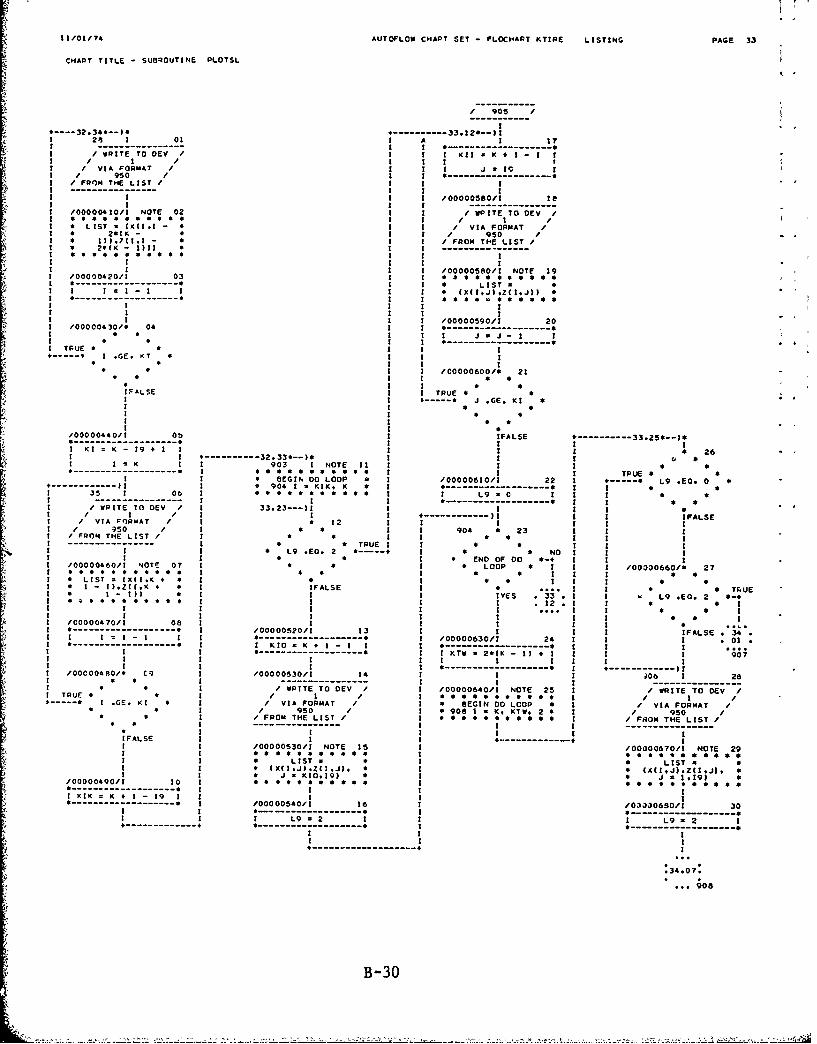
11/01/74 AUTOFLOW CHART SET - FLOCHART KTIRE LISTING PAGE 33
CHART TITLE - SUBROUTINE PLOTSL
/ 905 /
.... 32.34--....... .33.2 -- I
21 I 01 I A I I - I I 6---------!----
W/wRITE TOOEV / I I KIT - K + I - I I/ 1 / II I/ VIA FORMAT / I I J.V I
9 / 10 / I-- --------/FROM THE LIST I I I
-- - - - - - I I II I 1 /00000580/I leI I I
/00000410/1 NOTE 02 1 1 / WRITE TO OEV /
1 LIST s (X(I. - I / VIA FORMAT /1 21(K- • / 950 /I • 1))*711.1 - •4I / FROM TIE LIST /I . 2,1K - III) $ I
III I
I I /00000580/I NOTE 19/0000420/1 03 1-I-*-• 6----• •AS ------ * LIST 6I I - I * (X(IJ).Z(I.J)) 4---------- -1 I 66 6666
II I
I I I /00000590/I 20/00000430/s 04 1 -* 6 1 J.J-1 I
I 6------------ -TRUE* I I
. I ,GE. KT I I6 • I• I /00000600/6 21
'FALSE I I TRUE * ,I .....- J *GE. KI *
I •I 6 •
I I 6
/00000440/I 0 1 IFALSE --- 33.25--I*..------------------- I i II KI K - 19 f 1 I 1 1 1 26
I I ----------- 32.330--)1 1 1 0 *I I K 1 1 903 1 NOTE 12 1 I I6--------------------- * **6*• *6**0 * 1I I TPUE6 6
I I 0 BEGIN O0 LOOP Q I /00000610/t 22 1 *-- . L9 *EO. 0 6-II 6 904 1 KIK. K * ------------------ * I I a
35 I 06 1 **•66•6•6* I L90 I I 1 1----------------- I * ------------ I * *
/ RITE TO OEV / 33.23---)I I I I/I I I -- ---- I I I IFALSE
/ VIA ORMAT I * 12 £ II I I II / 50 / 1 * I 1 904 6 23 1 I IFQ04THE LIST/ 1 * 1 1 I
---------------- TRUE I * I I II I S L9 EO. 2 +-.... 16 NO I I II * I * END OF 00-6 1
/00000460/I NOTE 07 1 * I LOOP I 1 I /000030660/* 27*666•*66*66 1 6 £ * • I I * 6• LIST : (X(I*K £ 6 I6 I I 4 •
I 1-I).Z(I.K+ I IFALSE ... I I TFUEI - I IYES * 33 1 I L9 *EO. 2 6-+
I~~~~~I *4666* I1.21 1 1III I I i .... I * *
II I I * 1/00000470/I 08 I I I I I I*1 -------- I 100000520/1 13 I I I I IFALSE * 34
-I I-I--1 * !!!-------. I /0000630/ 24 1 I 1 01.----------------------- I............... -* 1 1 1
I 1 ................... I I KTW - 2*(K - 2) * 1 I 07I+ I I I II I 1 ... ... ... ... .. 1
/00000480/6 C9 1 /00000530/I 14 I 1 1 J06 I 28• * I . I I I. . .
I 1 / WRITE TO 0EV / I/00000640/I NOTE 25 I/ WRITE TO 0EVITRUE6 I I I / I *6666**66666 1 1.--.- I .GE. KI I / VIA FORMAT /I * aEGIN 00 LOOP I / VIA FORMAT
" * I / 950 / I 6 908 1 6 K. KTW. 2 I / 9506 6• I / FROM THE LIST / * 6 6 6 6 6 1 FIOM THE LIST /
6I III I6II I I I IIFALSE I I I -.....----- I
I 1 /00000530/1 NOTE 15 1 /00000670/I NOTE 29I 1 LIST 6 *
* LIST I I 6(XfI.J).ZcI.j). 0 I 6 MI.Jh.J. 6I IJ KIO.19) J = .119)
/0000490/I 10 I166*66664666 I 66666666666
-------- IIIKIKK = K I I - 19-------------- 6 1 /00000540/I 16 1 1033306S0/I 30
I I --------- * ---- - .------- *I I L9 - 2 1 I I L9 2 1
----- -----------II I
:34.07:... 908
B-30
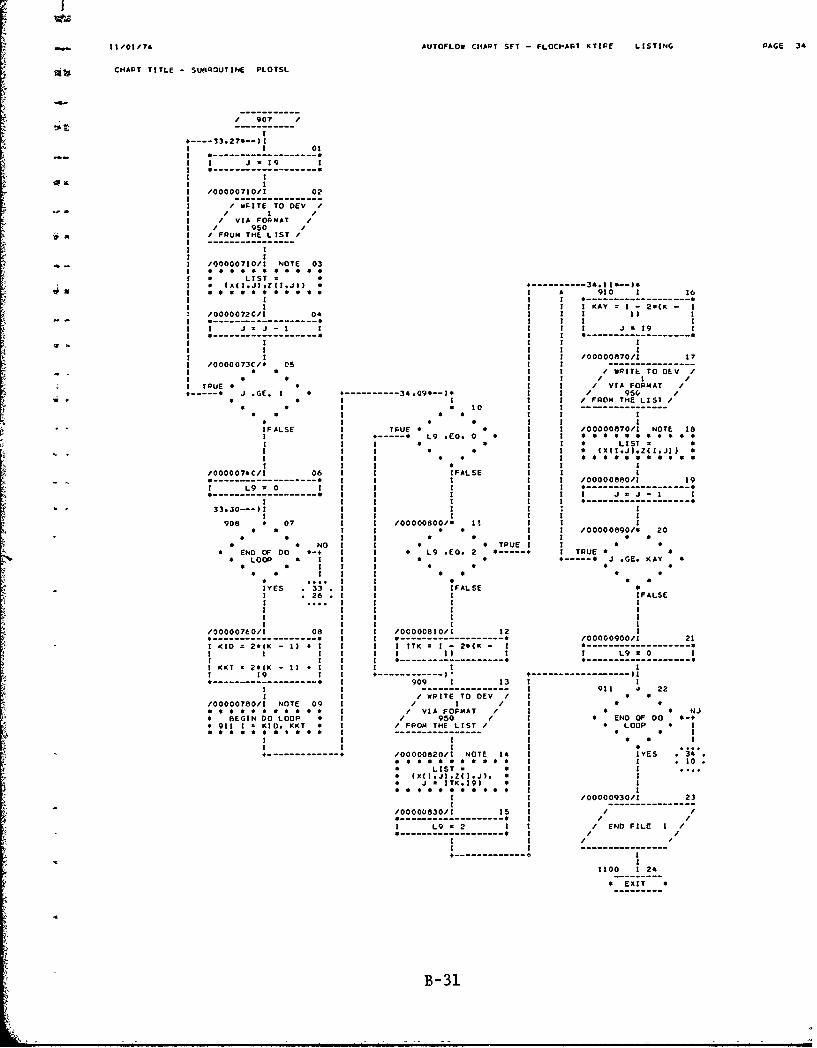
11/01/74 AUTOFLOW C14APT SFT - FLOCt-ART KTIRE LISTING PAGE 34
CHAPT TITLE - SURQOUTINE PLOTSL
/ 907 /
• ..33.276--)t
I 1 01
-----------
£ K J.z19 I
K IK /00000710/1 02
/ WGITE TO 0EV /
/ VIA FOPMAT // 950 /
I / FRUM THE LIST /
I K
_ I /00000710/1 NOTE 03
K S TLKST
I (x(I.lJIZ.(ItJi) - 34.11*-•K A'eel *ill i A 910 I 16
I I I -------------I I I KAY a I - 2*(K - I
/0000072C/i 04 I 1 I 1) 1
I I J zJ- - I I I J z 9 !
KI K
I /00000870/1 17/0000073C/! 05 I I
K * • I PITL TO DEV /• •K / I /
I TPUE * I I VIA FORMAT /---- J .E. I - ---- -34.090--It 1 / 950 /
• Ii1 I / FROM THE LIST/to I 1 I ----- -
A A • I
I FALSE 1TRUE I /00000870/1 NOTE 18I K ..... S LI9EO.0 1 I•* * •*
K * ILISTK (X(I.J.z(II.J3) S
K • • K K ••••••••SI I I L KEK
/0000074C/I 06 I I FALSE I I IS------- K..... . K I 1000080/I 19
I L9 0 K I Kt * -------•*-------...... I• I I J:J-1 K
I-I I K K --------33.30---)I I I I
I I I I I I908 1 07 K 1 /00000800/• 1 I I I
I I A /00000890/s 20• • * • • •
• • NO K• * TRUEK • •
• END OF DO -+ I L9 *EO. 2 *- + TRUE •Y• LOOP • I K • ---- J .GE. KAY
• • I K• * * •• • . . I * * •
IYES . 33 1 I [FALSE AI * 26 1 1 I IFALSEI *... I III K IKi I III I K
/00000760/1 08 1 I /00000810/K 12 1------------------ ....... /00000900/1 21I KID = 2*(K - I) A I I K TK K 2•(K ----------------------------------
I 1 K I II I I L9= 0 II I I .------------- - --------- S
1 KKT * 2*(K - 1I • i I £K 19 1 1 ----- -' --------- I------------- K 909 K 13 K I
I911 4 22I I/ WRITE TO 0EV
/0000078011 NOTE 09 / 1 1VIA FORMAT / K0 * NJ
* BEGIN DO LOOP I / 950 / K END OF DO •-+* 911 1 * KID. KKT • 1 / FROM THE LIST / I LOOP • 1FI K • * I
I K •K,,,
A-A /00000820/1 NOTE 14 I IYES , 340•• * ** K I . 10
S LIST - I I(X(I.J).Z(I.Jl. 1 I
J ITK.I9) I I
*S * S* * S I I1 /00000930/1 23
/00000830/1 15 /• • / /
I L9 c 2 I / ENO FILE I /----------- • / /
I! / /
I -
A------------I
1100 1 24
S EXIT S
B-31

m'1
APPENDIX C
A COMPUTER PROGRAM FLOW CHARTFOR COMPUTATION OF TOWED FORCE COEFFICIENTS
FOR PNEUMATIC TIRES
(Page 17 omitted)
4 4
C-1

1101
II I, A C, AU.P1LO (NW? CA T - P4LOCNAT RIS LISTING PAGE 01
COAST TITLE - INPOOUCI SI COI.NTS
TInS PROGRM COMUTCS TIE TOWING FORCE POP INPUT VALUES READ
FROM DATA FILES IN THL FCLtO.ING OROE
CCP OCONC INo1E GMAOINT IN LBS/CU IN)
CI I COl INDEX IN LOS/SO INS
PA 410f *OIUS IN PT I
00 1 IE IIW1IN IT I
LC I TIT LCO IN LOS I
PV I TI LIMIT PO lSSUl IN LAS/SO IN)
DE I DEFLICTION COEFFICIENT EPSILON )
FAsC 4 MATIM OP MA. INI[F. FRICTIO(N ANL. TO FRICTION ANIt1 I
A$ I RlAP ANGLE. INITIAL VMLUI ASUMED AS 10 DEGREES I
TALrAC I FACTR O FININ ZERO $HEAR SIRES$ LOCA4TIN I
Cf I COECIC% IN FRONT PILD I
LP I COHESIO IN P LDA9 P5.0 LOS/SO PTI
UP I PCTI0. *GL I :L o k ve P414L0 5
PA 4 PRI¢TI 401 AGIt 514 I[A hlELD IN 01011I$ I
,F I UNIT W1I444 IN FICNT FILD IN Les0/CU PT I
CO 4 UNIT WE IGH4T IN MEAl FIELD IN LAS/ CU FT I
.Al. VARIAtE OC.SICA.TIONS ARI
AAO. ElAT ANGLE IN MADIANS
AA SEPARATION AN[. IN RADIANS
AM- tA. ANGLE 1. 01GR11S
8* SETA COEFFICIENT P0 4L.OG. SPIRAL
01- INTERFACE FIX CT 104 ANGL41 IN A01ANS
PL. LIMITING PRESSURE IN IRS/so Pf
00 OTPOIIO TIll RADIUS
ODNF- COMPUTED LCAD
PIP. (015110I 109144k FORlCE
T?' C 0 UTID 0fwn
W*IN) M CENTRA. ANGLE 0P POINT N IN DEGREES
001k) 0 1C4N00 STRESS AT POINT N IN LB*S/2 PT
LE(NI - SIAR STRESS AT POINT k IN LBS/SO PT
WI6N) - I COODINATE OP POINT 14 VIT 4XIPRENC TO TIRE AXtS
V¥INI * Z COODOINAT OF POIATr 1 WITH PF1iRE1CC TO TIE AXIS
4AIN VAIASLE 0E(SIGNATIONS IN THE $0RI0ITINt API
Xl.JI * A C0RD5INATIS OP POINT IhJ
IIlJ4) * 2 COO*OINATES OF.POINT I.J
St.JI * SIGMA AT POINT 8.J
TI1.jI - THETA AT POINT IJ
AIJI * TANGENT OF DEFORMED CINTPILIIP& AT POINT J
OIJI * INTIPACI FRICTION ANGLE AT POINT J
C-2

- 110o/s4 AUTOLOV C .AT SET Ft0C.A, FInWS LS3146 PAGC O
CH&RT TITLE PROCCOuIRIS
I O
•" /iN' 91004 I 4 */ 4 IS I I..I ........... / 3I U
* - ~----- - ---- 1
I I * €1 .10. 0 *-.I I . A
A At O0 l IC LISTl O* l
/1011041,I 0.01t l I . I t
* LIST * COP C I. 4 I* hA. 00. L0. P0. 0 I PNSE . 3** oi. 0EAc. A00. * I * 41
041.104G CF: CO*E046 . * II 9* FC r * * I,w i. 2. AI .*-
I I Ii I00000760/I 09
I I100000410/! 03 I cO * I - cI I
A A A I I* * I I CC OR CO I
A . 1S I I0 ENO Of 0ATA I- 0 - *?5*CI 1A I I I IA A I I o I - PO I* * I I I I
I I G0 to II .10CsI .O *1 . I I II 13. I 0Go0 - Go I
I .399 II -- - - -- - - -- - -
I I II
CO PUTI ICOoSICk..F.ICTIO I 3.02.A G LE 0I o o C O e IPENETRATION 0ATA *. I0
III I
/00000640/I 04 1A I
A COO .... 0 *
ISIL•I*I 60.10-IFL5I O* - O
I1 50304AT M4,111/. I
I 64 - *.& tLOS) I
T -GO - 104 - II I*.5111 -I ILO)
I00000 I0/1 0
S tl[ OV I I I
II I7 h l IL O G I O ( C I I II I I331/100
I I I
I SI0 00 710 1/ it
I A I F 0
Aooo 00 /I 0 ? I .0 .• A IFAL-SE I-
I RI O Gl. 1.1 I -- e I A
A I I I 13
A I I --.... -
II0 00 0 . I
SOCOOSOS PI it?.oT )it II. III
I I "0 3.00.W
iII I
C313
, .,:3:: ,,k ,,. 'I o4* l eill IITS1 11Ct., N,
I T .0i i2: it
;0
~C-3
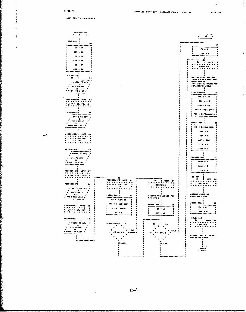
ISOS/y AUTOPLOW CHANT T . - FLOC"APT PAWS LISTING PAGE 043
CNANT TITLE PRentouS
...... 40 /ozo--- ----I ElII
10.0 I--- I .. .. .. ...
I cI I STI o * CR I I . . . I
I m- ----R I
3 l 5 I RY NOT
I - * T TO Ie I I a*CA 61 A * RI VIA0O. AT II I S EP G CON AINTA
II I
I.. .. I I
I £ F I .0 I O I
I P RI I
f I
0eO*lI I
O I 0I ASIGNE4 II. A£0 MA.... I.. 0...... VALNGS POGP ENTRY AN•
0040TO0E /A I £9 INITIAL. VALIE POP4i /0 *e~ I SEDAAAT3ON4 ANGLE
6 1
I/ VIA OR. T I I I
A l O IOI -OV I I
r~~~~~ ? 0 0 T T L S 00 00 1 30 1 30
I i I I I O Z ;Afe I
/0000 000!/ NOTE 035 I 1 00 N
* LIST * o. ,o. GO * I I A4 •0 60 1
I I I A * AR cAEMA I
3 IIIS I
1020004 /011 1I PSI * C 0 l03 I
WRITE TO DEv I6 1 II VIA FOR"MrT 100 200I/ 2R
IP RM EN LIST I I AN.... . . II I RMY. 0 tI I I 0I0X I
I I I
"000009 011 NOTE 0 1 I 1 IT 0 1
eeLIST CC FA C O
SLO . . . I I I*000000 •• * e* 3 I LOW * 0 3
NO Io I I o00 ITOq TO ORT / I • 544I 5
I s I
LIS 100 lENT C
I V03000940 I I I A
4 0841010. .. I I II FROM TH LIST I C P A I 1 ILIII P ITE 01
I AOR R O 0.0 7413 II I 1460 R0 " I s " STE 34" C N3
0000094011 0o I -- -I OIS- -I 00 01S CO 3 S 3. t o I..I... .
VA FRT TOAV / 0 .0 0 .0 .
- IA II I I IIT 1
/ VIA FOR•MAT I I• I•• •*e I I I I A €ON IMTINE
P 00001 T LIST I I CO I 0 A I. C * I I .- - - - -- -- I P-- - 1 I I I I
I I I II I /0 0 1 463 0I~~ $6 IAO C.lOO0IT40tR I /O0SSIG I 30~&L I ---O..-./OOO OVAO I N TE 0 I II I*--- ---- --- - .AISI I G PLM ITIN I
TLTC I.T 0 I I III NITII AL VALUE0 I I CFOR NSA I
I * -- -- -.141 . -. I I I I 3
I II
IIIII I I /00 0 4l ]il 1
IFLS
/00n009.I110 II I 0l I I I NOTEc-4
1000e960€ .T 09I I I .. .... I 3 0000000000:',, ITE TO 0, 9 /o1 I ,,.,109/ ... I I 30 o..3 I I , OIIILA A I 03 30 I I 000 000 00AOIPOOT 0 I I €0 0 3l I I... . . .
A I3 / SG REII 0 0 I SOJ EsINIILf AU
000 IOI I l0 I 0 . .. . 0 I I O8 t
3I I I e le•I'Vli O V 00lSS 1I 34 $I I /4.0N0[
I IT• 0•Le O. . I I I~ ~
........... •• 8S E IIT~C-4~t

*UTO'LO. C.-T ft, ftoc..., FoS ListZOG PACE 04
c "4n.* O TLE *S0Ct0uftes
03.25.- .
'000013410/1 01
I A. A 4.A
06.06~-11
54 * 02
FALSE
10 *
Iitpuf
I P AL
I i000ISS1"I 03I -- -----------
I II0 AO *.0* I *------I
I I
I SLOI I *AO
I /(COSCAAM/211
-- - ------/ -------
e000014504/. 05
FALSEat Gf7. fOAS S
I iv
1 001 DOOI 04
66 S. GSoO
.. !. ------ .
c-05
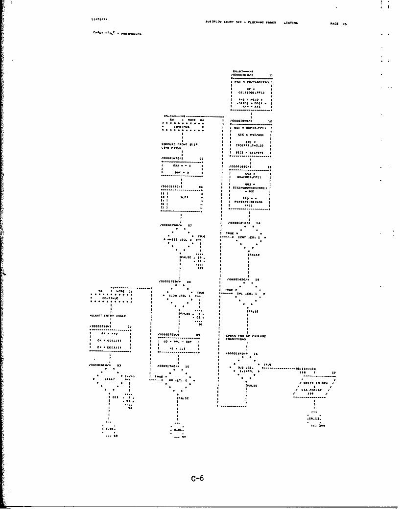
1303/14 AV0TLOV C.APT S|T-Lo P rp0S LISTING PAG
C"Of* TL0
- P€OCCOUgS
04O?---)./CO011S19./ II
PSI - CO"AN4I001 ) II I
I 02 IOI LTIDO0.PPII I
I 2I
I S10 0011 *- IAAI • AAI I
CS0 34-0ll ISS I 0070 004 /400030150/I Ii
. . .I . .I . . I I I
* COmlou1 I GUI * CIJPlC.OPII I
II SIG - 1si/Cu II I p • I
(O"PUT1 000T SLIP I I 101 Io.10..*OLIOG 013. II I
I SIGI - SIG.tPs II I • .........- ... ./00001600/I 0S I I
II II 00 - I I I 00050I I)
I ---------
0016 0 I0 I 1O01! I
TW II " I
/0000I100.IAI O I ISIO E*I I
7 II .. I ........ .
303wct 0402. I 0 .
II am aacj I I a; 1P1-0 of
I0 ecIl Ii IPI- ------------------
I - ---- 0 140-
I T II I O0061 Ie 1
AXC. GOI .T . 07 CF S ***st T e
;FAE .
03----- - --- I111 .
..T.. I .... • .T
I01S ** 34L
I .3 . I
309
? a : .. .. .. .... .
I e I II,•.o o,4C.oIC
/0O0011?0O/l 03 *• . .*X*IO I/O01l/ 0 9 I C flO m 0 AI
I .... .... ..... ... 4 € 4TI 0* CO OTI ovI~ * I o• C o I 0 0IU I IIx• lJ l I 4l * I I... I /0001 40/1 I
PO O 3~• 3 **0•4/e I 3 3* AI 0
3 00 I
I I PI Ill I
• C A*~ 111J1 I ... I O0 *~t 0J I I OO
I I I I I C 107 -- - -0 -- - - -Sl /0034/ * T:
I I 0• 3 I
/C O ISO . 03I /007. 30 0• 390. -
* * ** ST3 C
c-6

I CHAIO14 LUt~ft~w CI.I? 1 PLOrIMAT P 04 LI.TIN6 PAU so
CHAN? tI?3.l -f OIICIDuL
-.......
,=5. l I .. It
I AV O. AA 3
I 6v 0 1jijll II1 11 lll
IzI
< 0000100 0l8l O
* H
s 03
e *T . O 3~e40 l
3fs O) .............5 3 0G I .A A.. VV
G A - ----- -0-3 0 0
I I
3 010105 AICIOI -•el'O
3 I
003JJ3) MA PHI " 0001030/H! 003 A
t"(3JJ|I AI CHGPHL/00 3 H 0 3/0
P0JJ1 30 .OOY. AH. Y.qlT. I H I
I.H3 3 .03.
Hso
4.02.
49
-c-7

N7
tr
00
4[
a0
I-I
3
+0 OD. CL .+ OD f ,, ., ~
11j
ci L
+O
I-IIL ILI
I
I o
I
- I W -
Ic'jg 0 * - U
Q. v 0* *
10 IJ J
cc
a\Il
4L I I *
INI I 84

4*-*1 !
I
I II U,0
C) -- • i,---0
,.) ,0 ' 0 t, I - I 1*
I 0
, i JI I I
I I I I
I
II
I* I± .- S I

I 101078 LUTOFLOW C-1S SET - FLOCPAPT Fa S .. IST.. PAGE 08
C..A*£ TITLE - PBOC oU&E$
/ 79 / i 120 /
0.03-*-- NT 0---OTE-12I Wo o I N 2
0!!* I * 0
!A A
LIMIT CiLSSUF IS OT I COMPUTE INCAW FIL.OCOITA LPIPG I
I I I4I I002 W I3
"0002120/I 02 1. .
I PPL * Go, I - . . .............- eI ! I
I 32£. I IS•. . ........... PL ---- -- -- 17 . 1
5.OPP--I I AA - AiROARC
IO I OTE 03...... B.. .. S I
* CONTf |UE 5 • PA.E.B[ IS£A £A)4
. . . .* . . . . . I I I
I II I PAMI N I
I I Z COs(AA0 I
*0*0T FI D ICO.PUI AT .IoN It
I I II ./00002*S0fl IS
I U9 P Vyl jill a E PULSE
II o *T. *
a' * vw I *
* i - 3 I £ I IT U
OI 3
£ I
IDSO0210/I NOTE 05 I 00000050/I I6---------- '---- ..----
BEGIN 00 LOOP BI S * AIN £
* ££0.........I.-- - -
I.......... . . I
------ - ----------- I
..... ...... .... H"137V - I9N J UUI1 U9 Z9 £
O-OGI00N| -,00137 - IJ I Ioi
I 1 0ACOF - I
N EE () M 3700S - I ---- --- 0V9.0 1 1U 1
NOI 09*543-1
+ VVP+|• ¥17 -• G8"W DO LOOP I IV0000.3 * 11 h - I£ I 0 I
II I
£ - t 1 E- .............. AA- -- AAN I
I I NI I I I0I2 / AAN O ASI(B|J17 £ M .1 0 o 1B1
I£(I I 0 LOO I P 12
I -I AA0 AAI II Ito op I vv) 0 * ----- --- - .
:,• *UUINI 0 1 INo . . ... . ...... 0 £oooo Eso/i 19
---- OF 00 I- - - -1 A .
• L£ OP 1 1 1 1 £ £l OIPIOII II I I I I I
1[ 1 1* 11Z 1 1 P5, II I CCOTm.£I I
1 £ LOO £ ------ II S p£O(F 1 2UN 0 I.01
£1 .s p * - - ------ - £ / -0-0-5-0/ --£
-- -•-- - - I
I / 9,01
IeE I
£---------------
C-9

33/01/70 AUTIOPLOW CHAT SET - PLOCPTf TOMS LlS3136 PAG 09
€14j1 yIIL2 / 322 .j 2
I sic .
II
------- -- .
l o utg~ I O I sool [ I
I I 33
3IG 3 l3lll OGII *4
/0C 26 01341.1 0
33 • .. . .. . .. 3
T 1 uP* IU .CO 30 ) U IN. 3S0 3 I 3 O
IE.2 V0vld * 0 aI I 3
II
Tou I 3 0 5
3FLS I IOvI I N
I CIC' *00 No 'ILU*E3 I .
3 • I
3 ,ooeoz..o,. 0.....-------- OS0--I*
"ooo~sot aso I •
I 0 Tou I 0
3 TU 34* A I
II UUA 3
II
I I
I 00o0oo 601*e o ---
I ..... f --.. o1• o-,
I 3 xx .3
I . .. 3. . .00.0.60.1
- - - - - - - - - - - -*.00--o 3lfI DO000/ 9 03.0 LOOP 4 AA. A..0337 o I T u I 0 6 • IN 0
I .*o3•iA. p 3 3 0oooo61o/ Ol3 • I
X.. Ge" 2 6 *- I ---- I o £0.0u3
.......... • ... *•
31 1 h 1 3.2 3:
- ------ -- 34 I ;
I 006403 0 * • 4 0 3
1. 0 3 . I PI33 I I• f 0
T I I N 302oo.S[ Is• 3 .
3IE 3 A00 0. o I CHC3O III 0RSS CNTUE IN3II I I
4 3 SAIIL I -- ---- - --- - 3
4 l 4 3 I I I
II 3 * *..3 3 ,. . . . .. . .
IPALSE 0 I T I 3I 030027M0/ I 3*7 36I ... I * 01T 3 No3-0 - ---- -- 30 • •• 0 P .0 .Cop..
;30 .. .3t304103 10 0 $1 31
.O I.03. .30.03
330,+,, ,o..; ... ;
I I I I I I -10I

1,33/PA AuAOftC. (A SIA $ -. LCc- A , 0, LISINO 1lAGE 10
/ Z3 /
I N37 1 I I 0 I /00003310/t IS
* CON0| •AR A Ut * (000th - I 6 * (U0,0J(6| -
I IDOOO 0 Ii II fl3A 0(61 A I I I UT * SOA US I
I a, OO - I I I
S1f.rsst tO O(W.1. I I u li 1t•tI - 4 *I.OA5.?OWING FOCE AND II A I I UT(UOSItdtMI A
Iou 2.t oh.I I 1 1 U3*COStHl£I)II 143.1e4e61 I I -------------I I I tell. JIt)) I a
SO000290O1I 02 ------ ................ I0 /00003340/t 6 ----------- 0.10--1.-VI NSAAAP -JJt I II •..... ..... •30 I 2
I I 210OO31t0sI tO I 360 .I . . tS •N? - t t ......... * U .A~oOSIA*I - 3 otc T C. . .I ¥1-- V-- - II t I- U3 St---U II TO EV I6 F#Ivy - TVVIN - I II
VIA FORMATI I llima? It Te 3 £ 365 /
/000 0l NOTE 030 t * UTV3AI-A3All I / P4A3 TAC LIST #I I Aft * VVV£N - tot * I .........* so~th os LOOP t * I I (vvVt,. *l I £..COS~.Im i II* t6O N A 53. h A t I vmyl - IV 1(0(2 I I- - - - - - - - -
t- - -- - - - -I t -------------- T--2• ....... ; ....... • IO0024470fj NlOTE 22III I I tA . . .AAAA
. . . It o0003360• 17 * INT *I O 1 0000316011 It 1 - ------- I
-- ------- ---- I I---- ----- ----- I £ I At~hoII l kl-t * - ( -IN - - I I I I WAITE3TCOS I I
I t 3At I 11UUU( - tN I IHI t - /0304490t- /1
1 N3 1 ) 1e 1 1u i 11 It•Vl•v #
II £ I ( Itu. Is", "I I I - VIA FO AT /I 100 001 100IN I UUUtI- I)*Utz I 1 1 V2 £ I / 3TI . ---------............ 1 Is I I IS 3a1 .......... 1 3 11 16 1 1 ......... !!.......
II I I II . /000032001 12 1 V TO 37 1
* /OO(lT0fl 05 ----- ----- - - - - ------------ /300 Ne
£ A.IATV., * U hItN/3VVVII £ . . . . . . .I too I : I
xt V~lm lip19o as0
* U UtI) * UtO - II - £TA6IpJ£ 3 * A/O£i@0O@t330/ 30
9. 1 .I... ........- O I s .A I T ! 6 T O 1 0T a s£ I £ £13 *013-l I 3 A• A I £ VIA POANAT /1 .. I £ I 1 /1
I 160 * 06 £I £ ITS .....0.3...I A £ 100003280/I 3 I * 08 ........... I
I A £
I A) V I 19 E *.. t G
t0211# 17 0O 2
160 OF 00 £ tI I *3I A * lt * VII - A9 1 £ LIST : ITA I I 3 3 /03003420e! £ A A * A. .A 3 3AS * SOATIA3962 1 1 - -- I
*ICS £ I 3 I £ I
I 1 15 B 3 3 8 0 - 1 COT 1 COM£3TC St6AE
S,-- - -,..------ I--2l -- . . .-/0 000•1 0 3 I 1 SN! UJUtN3 0 11 A........... /0003280/£ 5A £
-- 0 £I - COAPA e COAPUT 0 I I JPO• N I A II 03 *IN0PUT6 A £ £ U0 LOAD- ------v 0 I I I 0006 -*3 I I TO.EANCE I
* TI - 0 I * /A - .SA 1 A I /0004560/11 NOT 28* 3 (N - Ill I £I 3 AAAAOA lAAAI I /00003660/A 20 : L.Is 00 LOOP A
I US - IVYVIP) - I 3• A I . N 30 36 A£ 6 0 * 3 I £ VVV - lioii I A A A A A A A A A C 8 A
IA 8 -A / LO - 0.IALO • .16.02---Itt£ I I A A I/00003130/t NOTE 08 £. . A A.A. .9
A * I
* 9
I.I A 8L
; A
I A I
I I.OSE A 363 I .01.
/11.06 1 3
C-11

2I al0t/I -UVTOLO- C"WT SET - P-4S0* L00 1 IST8ING PAG It
C4.Rv
TITLE P ROcEDURES
-0.-0---2-
*Tout 07
1 .. 0.2 1_12J!-20 -- ----• ~ ~ ~ 3 lsO AM -
...... . AIII , - 11.........* • 3 2 2 2 A* V.A* * 2 3 0 2 2 2 l 2 l IJII
4 I./2S 8 1 l
I0:1t.Sf *4 + A0IOF - 0 1"/012 2
2 2 *L202. ** I ,04 UA92II *L - I - I A"2 . A*C l 2
A *** 1 IOe5AND
2 O .... .. .... . ..
32 2 13 2, 1 290 1 1
/000043/l 07 4* 3 * .
*.3t0
O* . *--------&---lA-* I 2 8
2 21 A.3 1 I ,I * -A LT. 11.P I ;
* LS2 2 A
I SoI
1 * 2/0003030/. 24 ,,
* 80 .20. 4982*I * 9 2 4.0O*
* * 2 2 8O4U3T8 A0 * L0.0T to *- I I* * 2 I r501A08T10N A2.81[ TO 8 0 2
I I.. A. A IS I RA I
1 . • 1 + 1 IFAS Tpu I a-- --- - .... .. . I . ldw C.b l
. --- 1:0O 1 1032400091 to
* 8002.50J4tOO |? O+ - 0 1
a A
I00035100 0 1 LO GT*-..e
K l. CO. 0
I I I TRUE108.... 1 00003970/ 1. 1 1
1 0 I
I 2..0.. I1
90 / to I• 2 1 1 OA2 12O ,0*. ..... 1 1II
0 400*4 2" 2 2
2 /00 030 10/ A00003N - Io I
A- to ----- --
TRUE I A.-: A* a . 1
K1 CO 2 2- I -- -- --- - -- -- -
• 09 2 --.- 1 2 2 4 **82I 8
I,..9. 8 2A . ....... - -
I I
1 2 0 0L. G T . 0 . . . -- - 1
II
0 11 I ... 880I 1. 23
2 390 000 10 .*.l *0 .. 342 2 ..... . . .
2 10 0 8 .. . . . .. . . . 2 242 9I *• /..420/ 3
/l0003620/2 0:I A I . U1 TRUE
I • all
.... 2.2 .... 0 . 2
,,,,,9I48 . 2: 2.. ,+. ,._ 2
04.0 22
I 2
I 2I • 0 20101 I
*000310. 0 *. * 3.4.. 00.. .... ....
C-"2

AUICWLO C"W? S[ -FLOCHA5I FN9 LIST.I. -AGE 12
C-At, tITLE -fOCOU&rS
I'.II---,.
/00003520/I 03
I A.- I
I------III 02
! CIt * I I
/00003s*0/* 03
-,1 • 6 ---- - -- - -* . 3*I I 04
.. fig lo ofvITALIe / 6I / VIA POLAI - 300 -
I I
.11.03. .1609.
2? ... 1I
C-13

33SO3/74 AUTOLOV C ft, SET - P3LOCOAItT 7888 LI0 ,. ftIk 13
/ *06 1
A 03
ft G • k * OftU
A LO .4T. Sf --- - --------
f , It
1•.o.0o30o0 12
• . A A100 3st 04 FAS.......... 04 L f...... fO AS I 3 ft 6A A
/000036900 05 3
FAL ISE •ILO LT. A
8.0 F A t /00003780,1 13
IIt f I. I.. . . ... I I
1 14I AI I APt Aft * 4.F& I
I II /000036!0f! 06 I L+AM A - 3 8 - II - I - -O--MC-* G 3
I I
I I ALSEI A A
AA - (AAM . A , GT . A 5AA •I 6*O783.ll0 ftI ft
... !.OtAftCfaI A8---------- I A,. Pu
•/000037O/ft 0f 1
A 160 0
002 0I 36•I - -
A A I A.... .:A
I I 1 III - AX - 0
II I I0000372011 00 I A? * 0
I I Aft ft AfIftN
IIt---- -
3 I*--- - ------ ,
f I0 .14.01
..... AAm A A... 300
83------.A ftl.f fA nc A •,100003730/3 0, f
I AA f AtCftIAt 4 I ITtUC
0 I
3 00 I
ft------ft--f-- ft-ftI AX t 0 I
C 1
.141+,o 14

II/'A AUfOFLOWC6 SET -LPO.. T V.-5 LISTI. -AGE
C"&*T TITLE . PQOCEOUk(S
II* 05 *--II
SI l * ITIS I I
ItO
I
/00003060* 02
w !ft.'a20 r*. --- -* a 329 I 05
* /IRf TO EYVI100SW , 6 .5
I VIA F0RAT!41 I. 330 f
I I
I IloOOC36 1o 03 ..
* 9 .16.13._ exx • TRUE
0 9a .Co. 2 A-. ... 399
A A
I * I
- I T
1000oe801. 0.
A A
* A TRUA AM .eo. I -
A* I
I I$ .20.
I 52
C-15

AUTOPLOR CUARE SET -FLOCNART PRU5 LISTI " VA'C IS
CHART TIT L - 0*OCco &E s
/ 344 /
II1 I4---I1I NotE 05
* CONTINUE
I
LImIT ENTRY ANGLE
I
I/00040. I 1 6
-- - - --------- A
I ERAU * I2'I ARC4ITYISR I
e0000 0501M .0?
A A* 4 RTJE (MIN *NE. 0 4.
A A I -A A3 I ATE 13
I'.LSI .•Ul" A A IU1 22'I .22.1 II 347 II I *OJUST ENTRY A4 REARI I ANGLES FOR NEARLYOOO4060/ 08 1 CONSTANT NORMAL-- ;.......... I STRESSES
I FUERI I I I• ...-... -... I
A I /00004220,I 14
.. . .. . . .. . .II - o0 I •. . . . h l - l00 0 0 I 0 I ........... .--- - I -- I* * I I ... ... ..-
M U I I /FALSE 4 I I I / WRITE TO OCV* *• L *LT. " I 0004230/. I 6
A A A VIAPFONATA A A A R E. 0 A ----- 19
TITRU A A. LC. AI IAM IA M
A -..--- I AIO04100 I IFALSE
/0 0000. 0I1 0000407I I ... 3S--- - ---- I I 9FALSE 4 RE . E. A I
-. . AC R 4 201A 4 . ...........
I Il4- -L3 ~ - 44 rou AI IIT I AMX A I
&R LG. TWU A__I I A X. PI I WARE.Lo. 4 TRUED - - - -|• AOCOIAR + 20) ...... -- -- - - ------.......A I4AMA N
I 0 Ioooo41Mo/1I212 R 20/00004100/I 02 A I6 A
I- - - - - -.ARE - ARCA I.E.. TRU I EIF S A TRU I TRUE
203[ I+IA I IAR.GC.I I MI 40-, I0I I I 4I 4 4J[
I 4 e
I 03 I UIP S **I*.4...... .. ............ I 000040.0/I I LS IA .10I A 44.AoC 1,¢ 3 .- - - - -R IA
A R E . I I I 360-- -ARCI -I - I I . 0II IOTFUO
---- I------------ 2
/00 A04I20/. 04 I /0000427011 is
4-
- - - ---- I------ A A R M Y
4 lEN, .E0. I A II.SMAPII
I.SA*
I A4A - AI L AW -A RC I . 0 14 4 :2 •AO+ -AC4IIA0I I 4* RMI. I
ARC* AOCIA 0 •R A*ClIAR II II .22 I 22
I I
1.24. 4.02. * 4.02.
.1. 64
c-16
AUTOPLOM C"A*T ScT - FLOCPAPT rIws LISTIG PAGE 16
C"AST TITLE - 90Cg0961S
s 385
A I~- Io -------
10.29---I11 01
Ito *tjuw
33 0 A 0.
0 tho Of CIOV LOW0 0 I
L0 O I
*A
1/0006610/ 03
• 0000:620/1 0.
/ 0610 TO (,c // 6 /
f VIA 13906A /
1--T.[ LIST I
I
* LIST * sNK
I
COMP~UTE TOING FOP*CEAN TOsOucCOE
I|CIENTS4 • I
50 I/0000465011 06
I UN - STF/OF II II TON . II &TU/10 6I I
I *...--- I 6.09O--I AI I0
0060 0 ...................... I. I / 001l1 TO Clv// 0611T1 TO D19 / I / 6 /
6 / I I / VIA POMAT/ VIA F--AT I I I 4 633
- 39 I I / P-C-I LIST I*.1J0 IKt LIST I I I - -
-I III I III I a /0000.12l NOTC II/00094670,1 NOYc 0 A 0 A 0 0 0 0
•LIST . N:0 AJHk)* LIST - RPU N. N * I o000161. £11461. A. A . I I . .9AA9.. .0J 6I I I *V*(oIo....o
II II I IIP TOnG,)( €01791I1I..T I IINA.CLPTASL1 .ADJUS I 4446 * I?
OcDcAT COOPU TAT IONS I I
A,*4- ) E ..... •.......o)SI20 1 1 I -- 600 NOO 0
* &GIN 00LOOP I* • *0NNN3.
4 T 6.
'ItI i
•399 I OTO IS
* O V I N U I *
II
C-005 ,1
C-17JT

11101,7. AUICOLCO 000A0 SET - VOC1.,A0*T WP-05 LI0.I 4 PACE 14
C(AI TITLE 0*o$1. .( 1L,3 a
a -5-10, - il-
01 51.4-.12
I ,+rT02 2 000300/ | 09 I /0000510OI 2 2' /0100000/I 0.000 20: I - o l -..... I2 ----.--- IA A A I IAA . A AI . .A z. 31u.0 l - --------- - -------h --
* Sf I * * I. 0 * 2 2 3 - I I +IO0 03 II 2 * 00 .2 * 2. 0,. *2 2 01*10 I 000 II
II A .I (A A o 0 I - - -I 1.020 02 I * .... ... .... I....... 2.2.* I 2 2I 2 0P10.02 I 25
- --- G 20--- A
, .++.'.0 " , , ... 2 2 2 *I4 * - - e 2 * 0 2 20O......... A"
2 03 2 * • /0000190/I 2---------- .... I- -------- I• 2
2 O(I.JI.•0 2I I * LOOPI * I T3 - .?11 I I I I2 I 2 2 " .102 - 02V I -tl . I I S11l * 2 2l2 2(l.jI.*0 I 2 e 2 00 2 2 2 I 2I I A I ... I A I I T1I.jl SI 2T,I I 2 01 . . OA2T2TI. I a0I 2 l .l I 2 2 * O** I IIA.W020I I• ............ I.......
I 2 2 ... 2 2 022I 2 I 211.- /00 070I
2 o. I AM . 2ol 2lz I W I I....I...... I I .......... .2 A AT*
00$2 2I ? l 91W0) I I
l* * 2 2 2 2 2 I 0(0 .2.'
. .... .----.... -- 0. .I
00 * 0 2 S /04*0 10 2 2 I- - - - - - - -I2 A21 - 2
•0 | 1 - - - - -/000+/ i )o . ?1LIA.-2
* too I I 2 -0 I .25.02/0.00 I IA2-------------------
0 * * 2 0202 03502? I I ........... 2
WI I I .T o I 2 I a2 4 A 2"
.4 O0(1 2 I 2 IOOP.0 I l 22I 40 2?
S I 2/00 30/ I* A A
I A AI I I I A IEO. 2.0 D2 I 2 I I •0000063 A A A3 . 1 I ---------- -- A A0 0A 0 N I 2 I * * I *A Is .2.2 2.O
1
ive o0 CI -/OoO 1o1i 22O0601 II I IOWUOTI II"
I~ - THET VAUE ATo~) I00 0 0 3- - - - - - --
- --- 0-2-- -0--------01I I I I I; a '2-
* * o 2 1 a* I I- - ------ W0-- 12 I I 2 2I I I V 2 I I 2 -
lI E I 2 I I I0 1 2 / 11 I 2 0 0 0 30 2 2 00 C a:00 04 *IOWA 29./0 21 NOT 2 1 2 I ------ ------ 0 fA oo 6ES.
2 I U l * WI/A - 01/ I 2 | . W0C I 2 I0GA. ON
.5 TA. I I I N. I 2
I I I I A
I-- - - - - -2 2 I •- - --301 , 2 .N SI-IG I A
Io I 1 .. . . .... . 30
4 I 2C.0 * I /00000 - % 23 I I 10C 2 8• I I- - -,ARPO
----- --------------- I: Iooo@bl P0W2CIU 2 2
I - $tI I I I -- -- I--I I I 2............ I 2........SO/$ 0.0I 09I 0000080I 1 0 I I ---- --------- -0
I I0II 1 % : •0000 0 -I 00A 0 W..I
I 02 00 I00 t 2 2 0 - 0(0 2 2 a l~icj o A I I 18 1 244..11000 1
I a 1 1--.. 11 .......... 0-2 I EIW IIAOIIC 2 2II3 2 I a PIO 3 2000 I 29------ I .
SI I I I O -I )/C$I
I0 0 -.o. I 1 2 0 O1 O - 20 I I 0 1 . 0
I •2| I B " DI 1 -! 2
• •• • 6 | I CONDTINAT FRE IIT C
I I2* -I 2 0 OEL(OA.$I 2 l IO * I-- l
- - ---- -S .Ac. e 2 /9.02
.I0 I
SIJ • I•
100000C-08

+ I[$1/01/4 AUTJOLOW (.7 $07 - FLOCHAPT F0.S LISTSIG PAGE 29
("AAl TITLE - W12*0 40I00 SLFIIA 1 01°)/00000600/2 02 I 00000O0I 00O00 00
2 722.4 * TI * I * IIGI2N 00 LOOPe
I £72 - 711044 I * 0 0 1 4P2"J.
Pa I I I402/10 22 I 2 4202 •
IePOIP2.121~j.42.2 I 1 20.06 --- 1I
P00 0I (I * T
AI
.. I * 7012I I * 2 U .70 1£4 4
0 * 02 0 21
• LOOP•
I I I **
* * ! *
I I I* 1.0000* I It
I A I 0
I I IN/0000091011 03 1 1
I * ~0 * 2T------ T. .
II j III. le . I
2.it S US I
I
22 I a 002 5411.- it 2
.. . 0 l I I 2 ---
I02000 OAF 0O0000 / 0 12
I l| $1 2 $ 1 - 2 |
... 2..... 0..... ... I vI 2.4£~ -
- --------- I I
I I.2229 . $ZlS-2h0 £ 2............. ..II
1O000001701 0 U9 S.hJ Sl| ;;;.012001l to
-2------- I -- - - - -- - -
v A 2 1I 1 ' 2
Av•ll&S(OIII ;•
IIS. I1 - *05. 2 00001301^ a 3 J
VII I *----- -- -- A I
I I VO - (TI.t I" ZIIhJ - E) • f IA£* 2 I - I - I I x I
A 07.20 $II).T I I
I -/O. Z~ *J ... IE 2Sh1- XCI - IJ)I$V I
- - ....2......... .- -
I I I2I I I- - -0 ---- -1 - ---. ----- - -
I I I00 0 . /0000!230/1 27
l * L * 2 .. .. . .. .. .. I I & V - V3 2/ (I - 2 I£4220T$20221 -I0 2- I 2 2/hJ
0 .2 - . .... I 2 0000130ti 23 1 I --- .4 - *
I I I - -- - I I - 2,Jl(.42 -- I
2 O 0 2 2 0 * £722.4 2 2 22. - 2£ * 02e ) *
2 ---- VA---- - 2--- -I l I I 22 2
I 2 :T SI j I 2
0INE LO2 1405- 1- 1 2 . J -02.4
1 SI IS 2 -.-----..........
2 .. 2.I.0$.2 I 2.. . ... . ..... I..7
I lI
1 NOTE 06 2 18 AN 2I I E
. A . . * 2 . 2 I I /0001 2s 24S EI 0 LOOP I V 2 2 TANIT21 I ..... . .
s , 2 2 2 - 2I420I,1 - I -2.00 . . I 22.4 - 222 I
20.0O --- l El 07 1l x V2*xfS-l l
I A ....... . 0 "00 2$ 2 - - - - - - -l*. ....... ..... ... .0002..0/ 20
* 20 --$ 4* 2..... .. . .. 2 1$ $22. - 2 T- U 2 R N
II* * 2 0 0 2 2-0 1, . $
LIS
20:*S.0,: ..o
02 0 20•
•-- 0 I 2 24 ** 220 2* 204.I 4 . - - 0 I /0020i2
0- - - - 0 I-I2 0 *

AUTOFLON ("O SET . VLOC.0AT PIW$ LESIIEC PAM 20
( SOy TITLE -SUAT3TTV SI
,~o 335l- -I 326 /lN
$1'
A .16 09 1
5(3. E*E 'T I 3 AT*--*S TTE 0III3*
I 3. 3- H . eI 1,J " ...... . .. 00001550t• 16
SI2T $oh A 3 3 20 * OTOTSEAE 3 T TUtI I .... . . ..
- 3.0 1
3 03.43 * (UJS 3 "I 3 - * 3-* 6 Ut GOoR - 3
3 T•I *TEE/E2.TU85 I 0 V 3
1 10000 ,460- sT I
I A o . 0 *
10030133]0,1 t2 A3 AM 6 t. 3 .. 0TAo T A3
A02-3---------- - ------- 0 Z0GE.- A.
T A 3A 10 063
A A . o---S20{.I ....... . 20Ol--lT I I /8
02350, I?0 T I I LSE TT ag 06 O 3 I TI • e I T T TOlUT(VtS T T Ti I * Tl T [ 31 t...
I T n % 0 T-T .
A LOGO T I I 000016703 II T A
O T 3 I I TOT O I IIASA TFAT.STIflT b,.,*0(0(6~~l 3 [ .319. I I 79j• 0 I II
TAI * .ST(T3.J J- 3I ....It I .J(l.
.I ........---S325 3 22 z ' I I I
* TT2*.STEE(I .3- - - - - - - -T.....•.......... . 3
I 0 Is .4-3- . 1 ,-------- - -S10 S 3?S(,J-
A 3 A I IO 11 ( f .5T15 1G -
to0 I G T - 0 * 7 I I I----- ------ 90 • 0 2- - 3.3 - I 1 136 9
LToop0A0 T-.l uG I I 3-----0I100 0 3I GO * ATAOEC3/G23 I 3 GS T - VT( 0 TO - I
A T - - - --- --------- 3 3TE40 2 - 3.J - 3100001 - 011 ---- - - - -532 * .511511 - 3 TIES * * I 3 T 4 0 2O - 3
*3J * 511.2J( 3 I T 0? , /000015201T 1 3 3 3 3 24J 2TT - 3.4 -S.A.. A A a3 3I U I I 0 0 3
..T.T-
-- A .EOT - 3.0 0 1 3 TATNEG6153 I* .233 I 1000025.0/I 0s - -- 0-3
----T--T3----------* A*
SI2SIJ - 33 I 33 IPIE 3 LS/ 03030,Oa 20----- 3 I T 0
I A A FAS T
/00001300/1 05 a A M to. I T......2... . ... . . ... ,04. * 0 * $ . ..3 00 * 20511T53200 . .3• I t Ti 3
I 3 ... 222 1 /00001530/0 14 3 0 3I U9 T $i5 1 I T 0 3 3
3 0 7(J - I T 3 3 I
*.LT. C0 3 IA T 0
II AlIp - G? I II I.........O30/I 23-- 13 ----------
130 I 3
-- 0 3----- ....... .I Ali --- -- --
ATAN(GIIG?3 - A3l I
CI2I
C-20

535i4AUT0fL0W C -M8! SIT - LO0000Y P0085 LISTING, PAGE 21
00001630/* 01
---- 4? .0!. Alit
I
tO01 0 02
0 3
I I
G-M. - AI MI
oi II 0
1 '12 10,
--------- -- --- -- ----- -
I
MNI - itO
I 001150 H3- VI101 I
I
I t I/ I
I S5: I It
--- ---. - ----- ---
~-0IO010/ 05J
Ip. I 1.04 .J 3
Uts 4
CI 21

wraftew C.aTt get - FLC.I e*~wl LIU1 Od as
a a, as. a a 30 aTAla.ala- aI
af~lgO as a
:~ a.a: ; - . B
a,,nzs 99 1s 1 'I a as eI. ms
a" I I a a I IIIP e . a-I o-z~sja- a a Iaa a a..aIDlaaa..a - a a a
I a a till - tacit a a .as - aao12" as I a~asa a a . 6 1
la* I vs. *a aa: . "Lot a
at a4. tL aA41. aa a,. za a at aGists
* .. I. a ~ j :,.aai itC a .. aIA'uSx 2;.* a ..------ a,. aa~a -ea .... a a 3 e.aaj a a:9 a a aIa ~ ~~~~ ~~~ xa cscjac
a a a a a .no
a a acjatoja a a a. ..
a ~t Ilsl ae aIa.ca a a 63 .
03 . a9 a 9
. a aI - - . a* ... a jci-aa. a ... a.zsca
apavoollou. a a0402ls towa., rueaa .e . a a aa .e .~ 8.a ;
a~~~0A~~J 4-0. a1C.l.~"a aa ..a ~ ~ ~ ~ ~ L ac a a aaj-a a aa
a 03aa a
XX ..0 a a . *
L a t. a Z-. a . a Ja .6T. PL 0-. ..---- a*~~SAS II o.T a(J6a
* a a aa a. a assaII
a 2 .... a aa ....
a tao a a aa taC-22

VIrc.C 1SI-ftt vF q LSIC2I.- IT r
II.S~1 ~1 L~ i lt - ~ 22 L2I3 l1 2
12. 33
SS
J144610C-23
allPO C T Mt- l. 1 L3ITS-4 * .
C-Aar Tg?..g - ' S~~LPI
- .5
32.0 .1
A AI * .. I .
I*L~ ..
186Ot6,1 03
ISADUS L
.7*L~ IS.L
*C-2

P.L.G#I LT. -L
3 *3
* Ilout
ali CT. I
I o0tlkTO ro. 0?TU
IIgo
:27.21
* ... 174
* C-25

ISO~*AMTFlwL C~v SET - ftcC...i P8S1 LISTS-1 Mee N
* ca
.T. * 011A I2 %O~TC 02
A . . .a
I I U GO - 1f
a I aa
A A .9acc. 2.0
I I A A
*-S I .A *a 10( I9 .
.. R It '0 . 3. a a
a a 1IaA 0 I .g
Sa23.04:a
a A*FLS O.,A..eG~a *
aa ,!!* vA- ,o aa a a
a A
a Ia.
-c-2

sus-T UTOt.0. C.MI UT? - LOC".? p&W LISThI. PA" *
II
Ac.ZSS 0 1 10
I *.T i"TO
I@OL :10.W :
. . .. Y ..0 . .--.- -..-... .
1 000*123 a1
-------- . ........I
S~ ~~ ~ LT ..00 0.012
oJ Lt. 3
-----------------
L ..4.L:.
.L1.0.00 *
* c-27