Transportation Research Part F 43 (2016) 90–103

Contents lists available at ScienceDirect

Transportation Research Part F

journal homepage: www.elsevier .com/locate / t r f

Distinguishing patterns in drivers’ visual attention allocationusing Hidden Markov Models

http://dx.doi.org/10.1016/j.trf.2016.09.0151369-8478/� 2016 Elsevier Ltd. All rights reserved.

⇑ Corresponding author.E-mail address: reimer@mit.edu (B. Reimer).

Mauricio Muñoz a,b,c, Bryan Reimer a,⇑, Joonbum Lee a, Bruce Mehler a, Lex Fridman a

aMassachusetts Institute of Technology AgeLab & New England University Transportation Center, Cambridge, MA, USAb TU Munich, LMU Munich, Munich, GermanycUniversity of Augsburg, Augsburg, Germany

a r t i c l e i n f o a b s t r a c t

Article history:Received 26 October 2015Received in revised form 3 September 2016Accepted 18 September 2016Available online 17 October 2016

Keywords:DrivingGlanceTime seriesMachine learningVoice systemsVisual-manual interface

Driving is an intricate task where different demands compete for the driver’s attention.Current interface designs present novel multi-modal interactions that extend beyond tra-ditional visual-manual modalities. These new interaction paradigms have given rise toadditional subtask elements which call upon varying degrees of cognitive, auditory, vocal,visual, and manual resources. The draw on a larger number of resources has made demandassessment and optimization challenging. How these elements impact the driver’s visualbehavior may provide insight into the degree to which a vehicle’s user interface influencesattentional focus. This report addresses this question by approaching the problem from acomputationally predictive perspective. Data were drawn from two studies that capturedvisual behaviors of drivers during a series of radio tuning tasks using a traditional manualinterface and a multi-modal voice enabled interface during highway driving. Manual anno-tations of glance times and targets were compiled for each task period and then used totrain a predictive model. A statistical machine learning approach (Hidden MarkovModel) showed that manual radio tuning, voice-based radio tuning, and ‘‘just driving”behaviors result in fundamentally and predictably different strategies of visual attentionallocation. We report classification accuracies of over 95% for detecting the correct taskmodality within a 3 class classification framework, extending prior work to show that timeseries of glance allocations contain highly descriptive information that generalizes wellacross drivers of different ages, genders, and driving experience. Results suggest that differ-ences in glance allocation strategies serve as an effective evaluator of the visual demand ofa vehicle interface, providing an objective methodology for demonstrating that voice-basedtechnologies allow drivers to maintain a broader distribution of visual attention than thetraditional manual interface.

� 2016 Elsevier Ltd. All rights reserved.

1. Introduction

Driving has long been recognized as a set of dynamic and complex interactions with the environment, composed of infor-mation processing, action planning, and low level execution stages (Michon, 1985). New ways of interacting with the vehiclechallenge our traditional understanding of interface demand optimization that was based primarily on visual-manual inter-action. Results from a naturalistic driving study at the Virginia Tech Transportation Institute (VTTI) conducted for the

M. Muñoz et al. / Transportation Research Part F 43 (2016) 90–103 91

National Highway Traffic Safety Administration (NHTSA) suggest that performing visual-manual tasks while drivingincreases the probability of a safety-critical event by a factor of three (Fitch et al., 2013). The logical observation that driverscannot react on their own to events in the roadway if they are not looking at the road in the first place has been a majorargument for the development of voice-based interface options in the vehicle. The availability of voice interfaces is increas-ing rapidly - in 2012 37% of vehicles contained an embedded implementation of a voice recognition system, with projectionsindicating that this figure may rise to 55% by 2019 (IHS Technology, 2013). However, the extent to which this interactionparadigm is inherently more advantageous has been called into question. Work by Lee, Caven, Haake, and Brown (2001)and Strayer et al. (2013) reported increased cognitive load and longer driver reaction times for experimental implementa-tions of in-vehicle voice-based systems. Fitch et al. (2013), Reimer, Mehler, Dobres, and Coughlin (2013), Mehler et al.(2014), Reimer, Mehler, Reagan, Kidd, and Dobres (2016), and Mehler, Kidd et al. (2016), all show that common voice-based interfaces contain visual-manual subtask components. It is thus unclear how the visual-manual subtasks of avoice-based interface relate to traditional visual-manual interfaces that have been linked to increased likelihood of a crash.He, Zong, and Wang (2012) provide evidence to support the notion that there are intrinsic behavioral differences (e.g. driverdistraction profiles) between visual-manual and voice-based interactions modalities, even after accounting for parameterssuch as task duration. Furthermore, ongoing technological trends that seek to supersede traditional visual-manual interac-tions with interfaces that also draw upon auditory-vocal resources fail to provide an interaction alternative that compareswell with naturalistic driving in terms of driver performance (Just, Keller, & Cynkar, 2008; Sawyer, Finomore, Calvo, &Hancock, 2014). In short, these insights seem to suggest that the observable behavioral differences caused by these typesof interactions with the vehicle are not clear-cut and as of yet not comprehensively understood or defined.

Traditionally, human-machine interface (HMI) demand has been measured in a limited number of ways. These strategiesinclude measuring the total time visual attention is directed away from the forward roadway (National Highway TrafficSafety Administration, 2013) or to elements specific to the operation of the HMI (Driver Focus-Telematics WorkingGroup, 2006). These distraction indicators (total time off road, total glance time to device) have been used extensively inthe literature (Chiang, Brooks, & Weir, 2004; Donmez, Boyle, & Lee, 2009; Tijerina, 1999; Victor, Bärgman, Dozza, &Rootzén, 2013). While these measures are intuitive and have some demonstrated utility, a shortcoming common to bothapproaches is that they aggregate behavioral information over a given time span to a single number, disregarding usefulinformation sources such as transitions of glance allocations. They do not characterize the impact a given interaction hason how a driver distributes their attention across a broader driving environment over time, i.e. taking into account glancesthat may support the driver’s wider situational awareness. Specifically, this includes assimilating information from suchlocations as the side mirrors, blind spots, rearview mirror, and the instrument cluster. These differences in glance distribu-tions can be qualitatively observed in the glance transition matrices presented in Muñoz, Reimer, and Mehler (2015) in amore information rich form than is readily accessible in classic summary statistics such as total eyes off-road time for thesource datasets (Mehler et al., 2014; Reimer et al., 2013; Reimer et al., 2014).

Given a more mature driver behavior model, the quality of a vehicle’s interface might be measured by how well the dri-ver’s behavior pattern remains consistent with a baseline attentive driving style, unencumbered by non-driving relatedactivities. In essence, an optimal interface design may be one that minimizes the divergence of attention from how the driverwould be expected to perform if no secondary task was being engaged in. This report extends prior work by providing such acapable driver behavior model and presenting an approach through which the differences between any given set of driverbehaviors may be quantified (i.e. calculating the probability that an observed behavior is consistent with baseline driving orany other model of visual demand). More practically, this allows for a quantitative comparison of vehicle interfaces on thedegree to which they impact a driver’s overall allocation of attention, e.g. how compatible a particular HMI is with attentivedriving from the perspective of visual demand.

2. Background

This report builds on extensive research in the field of driver modeling using Hidden Markov Models, as well as on pre-vious work with glance-based measures of driver attentiveness. The primary contribution presented here consists in apply-ing the former modeling technique to the latter quantification of driver behavior. In order to place this contribution in ahistorical context, a brief overview is given on Hidden Markov Modeling in the driving context as well as on glance-basedbehavioral features.

Several studies including Victor, Bärgman, Dozza, and Rootzén (2013), Tijerina (1999), Chiang et al. (2004), Donmez et al.(2009), Liang, Lee, and Yekhshatyan (2012), and Tivesten and Dozza (2014) have focused on glance allocations as behavioralfeatures, aggregating them over time to analyze glance location distributions and durations in the context of risk assessmentand situational awareness. Only a small subset (Liang et al., 2012; Victor et al., 2013) have studied them in a time-sensitivecontext. Concretely, Victor et al. (2013) use glance behavior histories to explain risk from secondary tasks and perform ana-lytic work on the relationship between glance duration/location and vehicle crash risk. Corresponding metrics for risky andless risky glances are introduced, particularly in relation to the timing of lead vehicle closing kinematics. Liang et al. (2012)predict crash/near-crash risk using different combinations of glance duration, history, and location features as inputs tohand-crafted function-like feature detectors which output driver distraction estimates. Linear regression models were used

92 M. Muñoz et al. / Transportation Research Part F 43 (2016) 90–103

to arrive at model estimates, which allowed for an examination of the effects of each input on the final prediction result. Thereport found that glance history provided little benefit to the overall result (under the linear model).

Hidden Markov Models are statistical graphical models with a long history of time series data analysis. They work byquantizing the complexity within a system into a set of discrete states and a transition relationship between them (Oliver& Pentland, 2000). A thorough overview of Hidden Markov Models is given by Rabiner (1989). In the field of behavior infer-ence alone there have been multiple studies reporting their suitability for the problem (e.g. Ji, Wang, Li, & Wu, 2013;Mendoza & De La Blanca, 2007; Yamato, Ohya, & Ishii, 1992) and notably also within the context of driving by using vehicleperformance and position data (He et al., 2012; Krumm, 2008; Kuge, Yamamura, Shimoyama, & Liu, 2000; Kumagai,Sakaguchi, Okuwa, & Akamatsu, 2003; Liu & Pentland, 1997; Mitrovic, 2001; Oliver & Pentland, 2000; Pentland & Liu,1999). These works fall within the more general area of research that utilizes driver behavior models and machine learningapproaches to infer specific driving events and maneuvers such as lane changing, passing, and stopping (Chandrasiri et al.,2012; Chong, Abbas, Flintsch, & Higgs, 2013; Khaisongkram et al., 2008; Maye, Triebel, Spinello, & Siegwart, 2011; Qian, Ou,Wu, Meng, & Xu, 2010; Solovey, Zec, Garcia Perez, Reimer, & Mehler, 2014; Tango, Botta, Minin, & Montanari, 2010;Tchankue, Wesson, & Vogts, 2013).

In one of the earlier studies to apply Hidden Markov Models to the driving context, Pentland and Liu (1999) break down adriver’s behavior into different prototypical behaviors, each corresponding to an individual dynamic model. An unknownbehavior is then classified by choosing the model yielding the highest posterior probability. In other work, Kuge et al.(2000) build models using raw steering data (steering angle, velocity, and force) fed into a 2 level hierarchical HMM structurein order to infer the driver’s intended maneuver (lane keeping, emergency lane change, and regular lane change). The bottomlevel of the hierarchical structure is composed of maneuver-specific (in terms of the number of states and transitions) left-to-right HMMs, which were then linked together using a higher-level grammar (in terms of the number of sub-HMMs). A sim-ilar 2 level model is found in He et al. (2012), where the lower level encodes short term and immediate driving techniques,which are then organized in the higher level into long term driving strategies. Results were classified both offline and in real-time by feeding steering data into the sub-HMMs according to the grammar, and picking the composite model that maxi-mizes the probability of the input. The high recognition rates of this approach suggest that HMMs can infer complex behav-iors using unfiltered raw data directly, though other studies exist (Pentland & Liu, 1999) that show that an abstraction layerover raw data may be necessary for a high recognition rate.

Mitrovic (2001) presents another approach for driving event (turning, stopping, changing speed, etc.) detection. Filteredvalues from on-road driving periods, including average speed, average lateral and longitudinal acceleration, as well as accel-eration slope, were transformed into discrete values using a learned codebook. An HMMwas built for each driving event (fora total of seven). High classification accuracy was achieved on telemetry inputs alone by picking the HMM that bestexplained each test sequence. This lies in contrast to the claims laid out by Kuge et al. (2000) and Oliver and Pentland(2000), which state that the context of the input sequences is vital to the classification efforts.

Finally, Kumagai et al. (2003) suggest that HMMs may be considered as a tool for predicting driving events, much likeOliver and Pentland (2000), but with several important differences. Vehicle speed, acceleration, and brake pedal strokes weremeasured in an on-road experiment to train an HMM for anomaly detection. The goal is to predict the stop probability at anintersection on the order of 2–4 s instead of <1 s as in Oliver and Pentland (2000), using a hand-crafted probability functionabove the HMM layer. Though failing to specify traditional performance measures for anomaly detection such as F1 scores orreceiver operating characteristic (ROC) curves, the study provides an insightful correspondence between the actual and theprediction stop probability rates, even if only for a single participant.

Overall, as noted by He et al. (2012), current research in driver behavior inference very much revolves around the problemof detecting driving patterns and higher-order events given observed low-level telemetry data. The present work extendsefforts in this general area by considering the allocation of visual attention, in the form of glance allocation sequences, asan input to a predictive framework. An HMM classifier is used to infer the driver’s behavior in terms of their interaction stateand modality of task engagement with the vehicle. From the literature that has been explored, this is a novel application ofHMMs as predictive models in the driving context. As a case study designed to assess these concepts, this report examinesdata drawn across three key task types (a period of ‘‘just driving”, visual-manual radio tuning, and voice-based radio tuning)to assess differences in predictive performance. The work draws upon series of glance allocations during these periods ofinterest encoded as transitions of glance allocations and durations of allocations. Predictions based upon Hidden MarkovModeling are provided to assess three key questions: (1) Do key HMI design variables (such as task type) influence glanceallocation (transition probabilities/glance location sequencing) and thus the driver’s overall visual behavior pattern? (2) Howwell can different behavior patterns not only be quantified but consistently predicted given glance allocations as input fea-tures (that is, how well can visual glance patterns discriminate between behaviors and generalize across broad demographicsamples)? (3) How valuable are glance durations in addition to glance location features?

3. Classifying task modality and visual demand

There are three key elements in any machine learning framework that heavily influence its performance: the quantity ofthe data (Banko & Brill, 2001), the descriptive potential of the chosen features, and the model chosen to extract this discrim-inative potential. This report explores how well the combination of glance allocation features and Hidden Markov Models

M. Muñoz et al. / Transportation Research Part F 43 (2016) 90–103 93

works in order to infer driver visual behavior, drawing upon data from two studies with over 156 participants and 21,820glance transitions harvested from several distinct driving conditions. A three-class classification scheme is employed to dis-tinguish behaviors that are characteristic of ‘‘just driving” (baseline), visual-manual interactions with the vehicle’s interface(visual-manual radio tuning tasks), and interactions with the vehicle’s HMI using a voice interface (auditory-vocal radio tun-ing tasks).

3.1. Methods

Data were drawn from two on-road studies conducted by the MIT AgeLab to study the effects of production voice inter-faces in automobiles. The studies were conducted in a 2010 Lincoln MKS with factory installed voice-command systems(Ford SYNCTM for voice control of the phone and media connected by USB and the ‘‘next-generation navigation system” withSirius Travel Link). In each study, participants were asked to complete a series of visual-manual and voice-based tasks whiledriving on the highway (see Mehler et al., 2014; Reimer et al., 2013; Reimer, Mehler et al., 2014 for full details on experi-mental procedures and tasks). In brief, the first study examined a sample of younger (20–29) and older (60–69) driverswho were given structured training in how to complete each task in the most efficient manner supported by each interface;the default settings for the voice interface were used and these provided extensive audio prompting and required verbal con-firmation of commands. The second study set examined a sample of drivers equally distributed across four age groupings:18–24, 25–39, 40–54, and 55+, conforming to NHTSA’s recent recommendations for test samples (National Highway TrafficSafety Administration, 2013). This sample was composed of three subgroups: structured task training with default voice sys-tem settings, self-guided task learning with default voice system settings, and structured task training with ‘‘expert” modevoice settings. In the structured training, participants were taken step-by-step through the most efficient method of com-pleting each task in a practice session in a parking lot prior to the actual driving based assessment. For the self-guided group,during the parking lot training period, participants were provided with examples of the tasks they would be asked to com-plete during the drive and given the opportunity to explore on their own the respective voice and visual-manual interfacesfor completing each task type. The ‘‘expert” voice mode removed some of the verbose prompting provided in the defaultmode and removed verbal confirmation of most commands, shortening the overall duration of interaction. Table 1 summa-rizes the combinations of tasks and participant types for each study.

Each study included two trials of an ‘‘easy” visual-manual preset selection task (pressing a single pre-set station buttonlocated on the center stack), two trials of a ‘‘hard” visual-manual radio tuning task (multiple button presses and multiplerotations of a tuning knob to select a specified frequency using controls located on the center console), and engagement withthe same task end-goals using the voice-based interface (each voice-task required pressing a speech interface activation but-ton on the steering wheel, speaking one or more commands, and, except for the Study 2 expert mode subgroup, providingverbal confirmations). Note, when interacting with the radio through the voice interface, changes would occur on the videodisplay screen in the center console coinciding with selection of the radio and changing stations. Functionally, drivers did nothave to look at this screen, although they were free to do so. Thus, as is the case with most, if not all, current productionvoice-command interfaces, ‘‘voice” HMIs are perhaps most appropriately classified as voice-basedmultimodal interfaces thatinclude some visual-manual components as opposed to more traditional interface designs that are completely visual-manualin nature. The terms ‘‘voice” and ‘‘manual” are used here for ease of distinction.

Glance data were manually reduced based upon a frame-by-frame review of video from an in-vehicle camera directed atthe driver’s face according to the taxonomy and procedures outlined in Reimer et al. (2013) (Appendix F). The coding processinvolved the use of custom software (Reimer et al., 2013) that was developed (and subsequently open sourced, Reimer,Gruevski, & Coughlin, 2014) to classify glances into different bins. For Study 1 this included ‘left mirror’, ‘instrument cluster’,‘forward road’, ‘rearview mirror’, ‘center stack’, ‘right mirror’, and ‘other’; apparent blind spot checking and other head rota-tions in excess of approximately 90� were included in ‘‘other”. For Study 2, the bins consisted of ‘left blind spot’, ‘left mirror’,‘instrument cluster’, ‘forward road’, ‘rearview mirror’, ‘center stack’, ‘passenger seat’, ‘right mirror’, ‘right blind spot’, ‘other’,and ‘unknown’ (for video segments deemed uncodeable due to glare, video quality, etc.). The ‘other’ and ‘unknown’ cate-gories were infrequent and not included in the modeling. For analyses that merged data from both studies (see Section 3.2),the ’left blind spot’ and ’right blind spot’ locations coded in Study 2 were not used in the modeling stage.

Each task period of interest was independently coded by two different members of the research staff. Any discrepanciesbetween the two coders—the identification of conflicting glance targets, missed glances, or glance timings that differed bymore than 200 ms—were mediated by a third staff member (see Smith, Chang, Glassco, Foley, and Cohen (2005) for

Table 1Summary of participants and tasks for Studies 1 and 2. (V/M) represent ‘‘voice” and ‘‘manual” tasks, respectively. See text for addition detail on breakdown ofsubgroups in Study 2.

Study Baseline driving(V/M)

‘‘Easy” tasks(V/M)

‘‘Hard” tasks(V/M)

Participants(Total)

Trained/Self-guidedparticipants

Default/‘‘Expert”settings

1 2 (1/1) 4 (2/2) 4 (2/2) 60 60/0 60/02 2 (1/1) 4 (2/2) 4 (2/2) 96 64/32 64/32

94 M. Muñoz et al. / Transportation Research Part F 43 (2016) 90–103

arguments on the need for two or more independent raters). The duration of each glance was computed as a post-processingstep by taking the absolute time difference between its timestamp and that of the next glance.

3.2. Procedures

The final dataset was then constructed by mapping each mediated glance to the index of its bin, resulting in a list of dis-crete glance allocation sequences for each participant and task. From these, sequences pertaining to all 4 visual-manual radiotuning tasks and all 4 auditory-vocal radio tuning tasks were extracted and aggregated into manual and voice classes accord-ingly. ‘‘Just driving” data for each participant were taken from 2-min baseline reference periods preceding the visual-manualand auditory-vocal radio tasks.

Training and test data were derived from this dataset for the following combinations of the data in Study 1 and Study 2 inorder to test the effects of input data size on classification accuracy, as well as to test the model’s ability to generalize acrossstudies:

1. Training and testing data were derived from Study 1.2. Training and testing data were derived from Study 2.3. Training data were derived from Study 1 and validated with testing data from Study 2.4. Training data were derived from Study 2 and validated with testing data from Study 1.5. Training data were derived from Studies 1 and 2 and validated with testing data from Studies 1 and 2.

Concretely, training data were collected in each respective case by randomly sampling 80% of the participants from thedata pool and using all of their corresponding glance sequences. This was carried out in two different ways. In the firstinstance, glance sequences were created by matching each participant with all of their glances according to type of task(baseline, manual, or voice). For example, in the case of the four trials (2 easy and 2 hard) of visual-manual radio tuning,all glances across these trials were combined into a single glance allocation sequence per participant. In the second approach,each participant was matched with a particular, individual task trial. In this case, four distinct sequences resulted per par-ticipant. This results in an evident tradeoff: building longer, fewer sequences results in samples that are intuitively moreexpressive and thus potentially easier to classify. Building shorter, more numerous sequences results in more realistic sam-ples. Results are presented for both variants, primarily to illustrate the theoretical feasibility of the problem in the formercase, as well as the classifier’s performance in a more realistic scenario in the latter case.

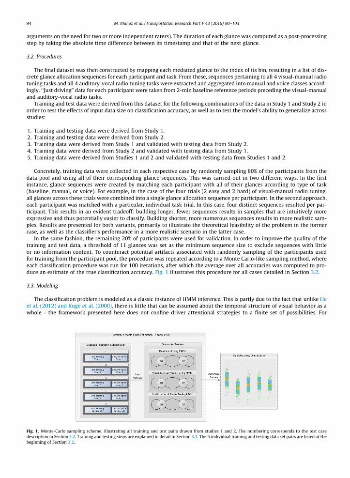
In the same fashion, the remaining 20% of participants were used for validation. In order to improve the quality of thetraining and test data, a threshold of 11 glances was set as the minimum sequence size to exclude sequences with littleor no information content. To counteract potential artifacts associated with randomly sampling of the participants usedfor training from the participant pool, the procedure was repeated according to a Monte Carlo-like sampling method, whereeach classification procedure was run for 100 iterations, after which the average over all accuracies was computed to pro-duce an estimate of the true classification accuracy. Fig. 1 illustrates this procedure for all cases detailed in Section 3.2.

3.3. Modeling

The classification problem is modeled as a classic instance of HMM inference. This is partly due to the fact that unlike Heet al. (2012) and Kuge et al. (2000), there is little that can be assumed about the temporal structure of visual behavior as awhole - the framework presented here does not confine driver attentional strategies to a finite set of possibilities. For

Fig. 1. Monte-Carlo sampling scheme, illustrating all training and test pairs drawn from studies 1 and 2. The numbering corresponds to the test casedescription in Section 3.2. Training and testing steps are explained in detail in Section 3.3. The 5 individual training and testing data set pairs are listed at thebeginning of Section 3.2.

M. Muñoz et al. / Transportation Research Part F 43 (2016) 90–103 95

instance, whereas Kuge et al. (2000) model lane changes as a composition of necessarily sequential events (expressed withleft-to-right HMMs, so called non-ergodic models in Rabiner, 1989), no such restriction is made here, allowing the model tonaturally learn any such pattern during training. Another reason for the simple architectural choice is to provide a baselinemodel for future studies that might expand in this direction.

In the present study, one HMM was trained per class. Experimenting with different model topologies showed n = 2 to bethe optimal number of states. One common problem often encountered during HMM training is estimating probabilities foruncommon emissions and transitions that might not be represented in the training set (i.e. just because the input data con-tains no glance allocations to the ‘right mirror’ does not mean these allocations will certainly never happen). Most imple-mentations of the training algorithm provide a way to counteract this effect by specifying prior pseudo-emissions andpseudo-transition counts, i.e. letting the model know that even extremely unlikely observations may occur in the future.Experiments found performance was most stable by specifying minimal, non-zero counts for emissions that did not appearin the training data. A uniform distribution was chosen for the pseudo-transitions prior. This corresponds to a Laplacesmoother, which has been shown to work well in Bayesian inference systems (He & Ding, 2007). This was done for the fol-lowing reason: each HMM is modeled with a fixed number of states that do not carry an application-specific semantic value,i.e. the number of states is simply another parameter of the model which is tuned with a validation set. This corresponds tothe traditional framework for training HMMs for multi-class classification (Kuge et al., 2000; Oliver & Pentland, 2000;Rabiner, 1989). The transition patterns between these artificial states are therefore unknown a priori, hence the additive,unbiased smoothing.

Given this set of trained models (one each for baseline driving, auditory-vocal radio tuning, and visual-manual radio tun-ing), a new sequence of glances is assigned to one of these classes by testing each HMM and picking out the model that pro-duces the highest log probability for the input sequence. Intuitively, the model is chosen that best interprets (and is thusmost likely to have generated) the new test sequence. Performance metrics are given in accuracy as the percentage of cor-rectly classified sequences.

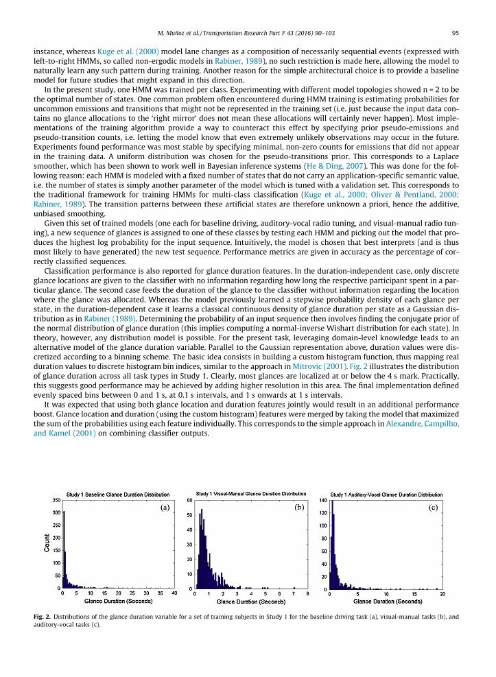
Classification performance is also reported for glance duration features. In the duration-independent case, only discreteglance locations are given to the classifier with no information regarding how long the respective participant spent in a par-ticular glance. The second case feeds the duration of the glance to the classifier without information regarding the locationwhere the glance was allocated. Whereas the model previously learned a stepwise probability density of each glance perstate, in the duration-dependent case it learns a classical continuous density of glance duration per state as a Gaussian dis-tribution as in Rabiner (1989). Determining the probability of an input sequence then involves finding the conjugate prior ofthe normal distribution of glance duration (this implies computing a normal-inverse Wishart distribution for each state). Intheory, however, any distribution model is possible. For the present task, leveraging domain-level knowledge leads to analternative model of the glance duration variable. Parallel to the Gaussian representation above, duration values were dis-cretized according to a binning scheme. The basic idea consists in building a custom histogram function, thus mapping realduration values to discrete histogram bin indices, similar to the approach in Mitrovic (2001). Fig. 2 illustrates the distributionof glance duration across all task types in Study 1. Clearly, most glances are localized at or below the 4 s mark. Practically,this suggests good performance may be achieved by adding higher resolution in this area. The final implementation definedevenly spaced bins between 0 and 1 s, at 0.1 s intervals, and 1 s onwards at 1 s intervals.

It was expected that using both glance location and duration features jointly would result in an additional performanceboost. Glance location and duration (using the custom histogram) features were merged by taking the model that maximizedthe sum of the probabilities using each feature individually. This corresponds to the simple approach in Alexandre, Campilho,and Kamel (2001) on combining classifier outputs.

Fig. 2. Distributions of the glance duration variable for a set of training subjects in Study 1 for the baseline driving task (a), visual-manual tasks (b), andauditory-vocal tasks (c).

96 M. Muñoz et al. / Transportation Research Part F 43 (2016) 90–103

4. Results

Table 2 shows classification results (average accuracy) for Study 1, Study 2, and both studies combined for 100 iterationsof the Monte Carlo estimation. Glance location, duration, and merged features were used. Two duration models are pre-sented - the standard approach based on a Gaussian distribution of duration, as well as the histogram binning approachdetailed above. Sequences were formed by taking glances according to the type of task (baseline, voice, and manual tasktypes). Table 3 presents the corresponding classification results, but using individual task trials to build sequences instead.

As can be seen in the tables, using glance location features results in high accuracy values, especially when buildingsequences from task types (Table 2). Over 95% accuracy is achieved using data from Study 1. As expected, compromisingon sequence length (Table 3) results in a slight drop in performance, implying that the HMM classifier benefits from length-ier, more expressive sequences. High accuracy values on the cross-study data sets are highly suggestive of general behaviorpatterns, independent of driver demographic or training. Duration features also show strong performance well above that ofa random classifier. Leveraging domain-level knowledge using histogram-based duration features improves performance inevery case, sometimes quite significantly. This strongly supports the idea that glance duration is also a key signal of the dri-ver’s visual behavior and that task modality may also be characterized by how long the driver decides to allocate attentionregardless of where. As expected, merging features leads to an additional performance boost which for the most part outper-forms glance location features alone, particularly when aggregating glances by individual tasks (Table 3). This suggests thatsupplementing these features with each other leads to a stronger predictive signal which the HMM is able to pick up andrespond to.

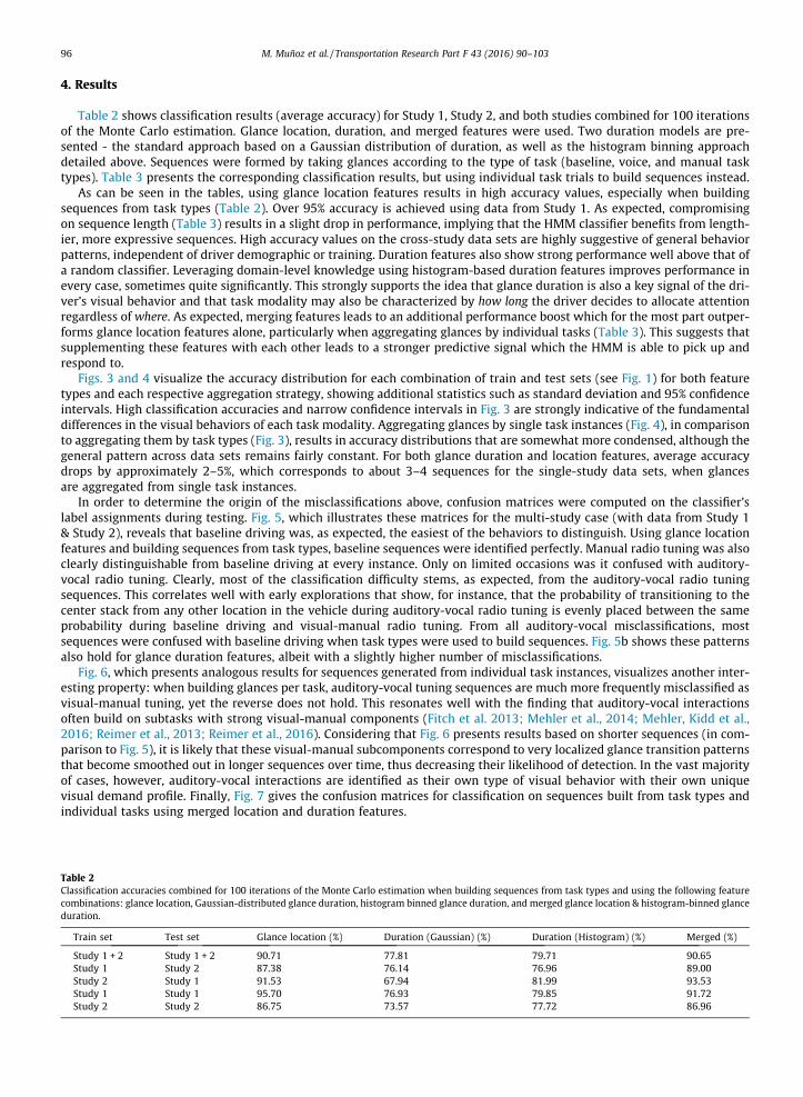
Figs. 3 and 4 visualize the accuracy distribution for each combination of train and test sets (see Fig. 1) for both featuretypes and each respective aggregation strategy, showing additional statistics such as standard deviation and 95% confidenceintervals. High classification accuracies and narrow confidence intervals in Fig. 3 are strongly indicative of the fundamentaldifferences in the visual behaviors of each task modality. Aggregating glances by single task instances (Fig. 4), in comparisonto aggregating them by task types (Fig. 3), results in accuracy distributions that are somewhat more condensed, although thegeneral pattern across data sets remains fairly constant. For both glance duration and location features, average accuracydrops by approximately 2–5%, which corresponds to about 3–4 sequences for the single-study data sets, when glancesare aggregated from single task instances.

In order to determine the origin of the misclassifications above, confusion matrices were computed on the classifier’slabel assignments during testing. Fig. 5, which illustrates these matrices for the multi-study case (with data from Study 1& Study 2), reveals that baseline driving was, as expected, the easiest of the behaviors to distinguish. Using glance locationfeatures and building sequences from task types, baseline sequences were identified perfectly. Manual radio tuning was alsoclearly distinguishable from baseline driving at every instance. Only on limited occasions was it confused with auditory-vocal radio tuning. Clearly, most of the classification difficulty stems, as expected, from the auditory-vocal radio tuningsequences. This correlates well with early explorations that show, for instance, that the probability of transitioning to thecenter stack from any other location in the vehicle during auditory-vocal radio tuning is evenly placed between the sameprobability during baseline driving and visual-manual radio tuning. From all auditory-vocal misclassifications, mostsequences were confused with baseline driving when task types were used to build sequences. Fig. 5b shows these patternsalso hold for glance duration features, albeit with a slightly higher number of misclassifications.

Fig. 6, which presents analogous results for sequences generated from individual task instances, visualizes another inter-esting property: when building glances per task, auditory-vocal tuning sequences are much more frequently misclassified asvisual-manual tuning, yet the reverse does not hold. This resonates well with the finding that auditory-vocal interactionsoften build on subtasks with strong visual-manual components (Fitch et al. 2013; Mehler et al., 2014; Mehler, Kidd et al.,2016; Reimer et al., 2013; Reimer et al., 2016). Considering that Fig. 6 presents results based on shorter sequences (in com-parison to Fig. 5), it is likely that these visual-manual subcomponents correspond to very localized glance transition patternsthat become smoothed out in longer sequences over time, thus decreasing their likelihood of detection. In the vast majorityof cases, however, auditory-vocal interactions are identified as their own type of visual behavior with their own uniquevisual demand profile. Finally, Fig. 7 gives the confusion matrices for classification on sequences built from task types andindividual tasks using merged location and duration features.

Table 2Classification accuracies combined for 100 iterations of the Monte Carlo estimation when building sequences from task types and using the following featurecombinations: glance location, Gaussian-distributed glance duration, histogram binned glance duration, and merged glance location & histogram-binned glanceduration.

Train set Test set Glance location (%) Duration (Gaussian) (%) Duration (Histogram) (%) Merged (%)

Study 1 + 2 Study 1 + 2 90.71 77.81 79.71 90.65Study 1 Study 2 87.38 76.14 76.96 89.00Study 2 Study 1 91.53 67.94 81.99 93.53Study 1 Study 1 95.70 76.93 79.85 91.72Study 2 Study 2 86.75 73.57 77.72 86.96

Table 3Classification accuracies combined for 100 iterations of the Monte Carlo estimation when building sequences from single task instances and using with thefollowing feature combinations: glance location, Gaussian-distributed glance duration, histogram binned glance duration, and merged glance location &histogram-binned glance duration.

Train set Test set Glance location (%) Duration (Gaussian) (%) Duration (Histogram) (%) Merged (%)

Study 1 + 2 Study 1 + 2 83.39 73.51 76.22 88.65Study 1 Study 2 83.67 66.37 73.61 87.64Study 2 Study 1 84.49 58.11 78.37 91.11Study 1 Study 1 86.89 73.85 78.11 91.11Study 2 Study 2 81.79 70.15 71.99 85.27

Fig. 3. Accuracy distributions for every train and test set combination using (a) glance location features and (b) glance duration features (histogram) whenusing task types to build sequences. Average number of trials (sequences) is given for each train and test set pair. 1 standard deviation is represented by thelarger rectangular box, the 95% confidence interval by the lighter internal box, and the mean by the horizontal line.

Fig. 4. Accuracy distributions for every train and test set combination using (a) glance location features and (b) glance duration features (histogram) whenusing individual tasks to build sequences. Average number of trials (sequences) is given for each train and test set pair. 1 standard deviation is representedby the larger rectangular box, the 95% confidence interval by the lighter internal box, and the mean by the horizontal line.

M. Muñoz et al. / Transportation Research Part F 43 (2016) 90–103 97

5. Discussion

This report presents a methodology for assessing the quality of an HMI in terms of the visual demands it imposes on dri-ver behavior. This assessment builds on the logical assumption that the driver has the potential to be most aware of his or

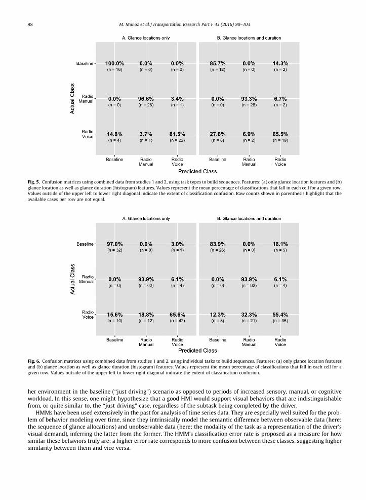
Fig. 5. Confusion matrices using combined data from studies 1 and 2, using task types to build sequences. Features: (a) only glance location features and (b)glance location as well as glance duration (histogram) features. Values represent the mean percentage of classifications that fall in each cell for a given row.Values outside of the upper left to lower right diagonal indicate the extent of classification confusion. Raw counts shown in parenthesis highlight that theavailable cases per row are not equal.

Fig. 6. Confusion matrices using combined data from studies 1 and 2, using individual tasks to build sequences. Features: (a) only glance location featuresand (b) glance location as well as glance duration (histogram) features. Values represent the mean percentage of classifications that fall in each cell for agiven row. Values outside of the upper left to lower right diagonal indicate the extent of classification confusion.

98 M. Muñoz et al. / Transportation Research Part F 43 (2016) 90–103

her environment in the baseline (‘‘just driving”) scenario as opposed to periods of increased sensory, manual, or cognitiveworkload. In this sense, one might hypothesize that a good HMI would support visual behaviors that are indistinguishablefrom, or quite similar to, the ‘‘just driving” case, regardless of the subtask being completed by the driver.

HMMs have been used extensively in the past for analysis of time series data. They are especially well suited for the prob-lem of behavior modeling over time, since they intrinsically model the semantic difference between observable data (here:the sequence of glance allocations) and unobservable data (here: the modality of the task as a representation of the driver’svisual demand), inferring the latter from the former. The HMM’s classification error rate is proposed as a measure for howsimilar these behaviors truly are; a higher error rate corresponds to more confusion between these classes, suggesting highersimilarity between them and vice versa.

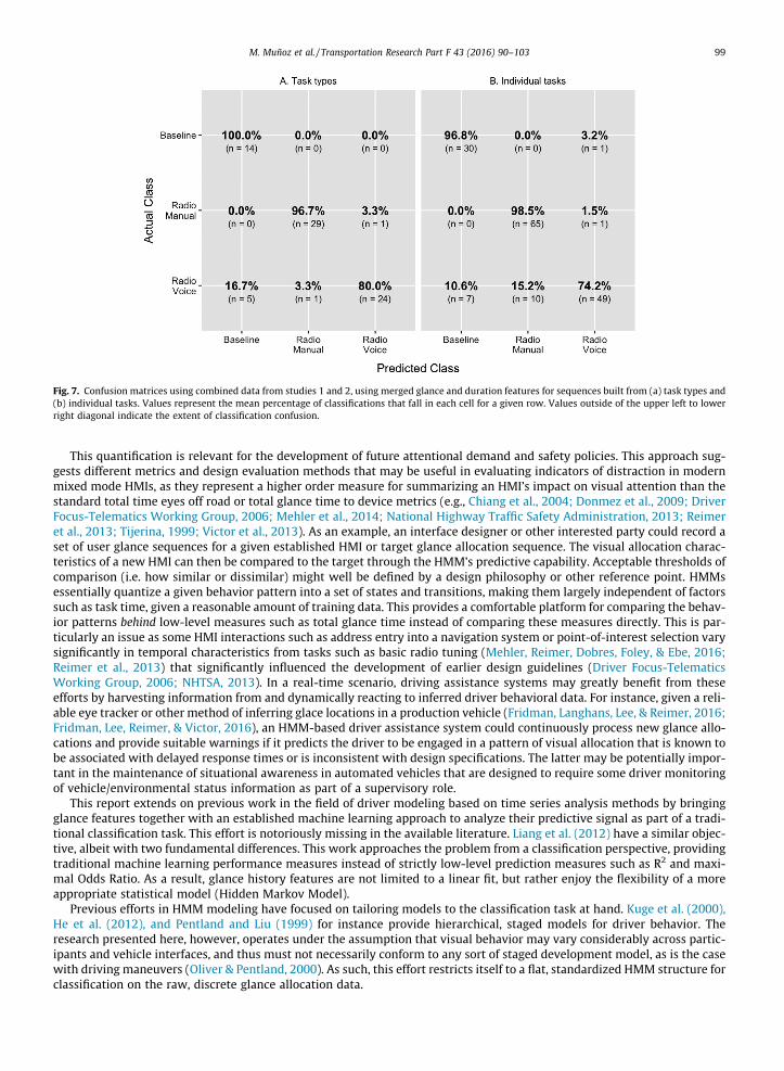
Fig. 7. Confusion matrices using combined data from studies 1 and 2, using merged glance and duration features for sequences built from (a) task types and(b) individual tasks. Values represent the mean percentage of classifications that fall in each cell for a given row. Values outside of the upper left to lowerright diagonal indicate the extent of classification confusion.

M. Muñoz et al. / Transportation Research Part F 43 (2016) 90–103 99

This quantification is relevant for the development of future attentional demand and safety policies. This approach sug-gests different metrics and design evaluation methods that may be useful in evaluating indicators of distraction in modernmixed mode HMIs, as they represent a higher order measure for summarizing an HMI’s impact on visual attention than thestandard total time eyes off road or total glance time to device metrics (e.g., Chiang et al., 2004; Donmez et al., 2009; DriverFocus-Telematics Working Group, 2006; Mehler et al., 2014; National Highway Traffic Safety Administration, 2013; Reimeret al., 2013; Tijerina, 1999; Victor et al., 2013). As an example, an interface designer or other interested party could record aset of user glance sequences for a given established HMI or target glance allocation sequence. The visual allocation charac-teristics of a new HMI can then be compared to the target through the HMM’s predictive capability. Acceptable thresholds ofcomparison (i.e. how similar or dissimilar) might well be defined by a design philosophy or other reference point. HMMsessentially quantize a given behavior pattern into a set of states and transitions, making them largely independent of factorssuch as task time, given a reasonable amount of training data. This provides a comfortable platform for comparing the behav-ior patterns behind low-level measures such as total glance time instead of comparing these measures directly. This is par-ticularly an issue as some HMI interactions such as address entry into a navigation system or point-of-interest selection varysignificantly in temporal characteristics from tasks such as basic radio tuning (Mehler, Reimer, Dobres, Foley, & Ebe, 2016;Reimer et al., 2013) that significantly influenced the development of earlier design guidelines (Driver Focus-TelematicsWorking Group, 2006; NHTSA, 2013). In a real-time scenario, driving assistance systems may greatly benefit from theseefforts by harvesting information from and dynamically reacting to inferred driver behavioral data. For instance, given a reli-able eye tracker or other method of inferring glace locations in a production vehicle (Fridman, Langhans, Lee, & Reimer, 2016;Fridman, Lee, Reimer, & Victor, 2016), an HMM-based driver assistance system could continuously process new glance allo-cations and provide suitable warnings if it predicts the driver to be engaged in a pattern of visual allocation that is known tobe associated with delayed response times or is inconsistent with design specifications. The latter may be potentially impor-tant in the maintenance of situational awareness in automated vehicles that are designed to require some driver monitoringof vehicle/environmental status information as part of a supervisory role.

This report extends on previous work in the field of driver modeling based on time series analysis methods by bringingglance features together with an established machine learning approach to analyze their predictive signal as part of a tradi-tional classification task. This effort is notoriously missing in the available literature. Liang et al. (2012) have a similar objec-tive, albeit with two fundamental differences. This work approaches the problem from a classification perspective, providingtraditional machine learning performance measures instead of strictly low-level prediction measures such as R2 and maxi-mal Odds Ratio. As a result, glance history features are not limited to a linear fit, but rather enjoy the flexibility of a moreappropriate statistical model (Hidden Markov Model).

Previous efforts in HMM modeling have focused on tailoring models to the classification task at hand. Kuge et al. (2000),He et al. (2012), and Pentland and Liu (1999) for instance provide hierarchical, staged models for driver behavior. Theresearch presented here, however, operates under the assumption that visual behavior may vary considerably across partic-ipants and vehicle interfaces, and thus must not necessarily conform to any sort of staged development model, as is the casewith driving maneuvers (Oliver & Pentland, 2000). As such, this effort restricts itself to a flat, standardized HMM structure forclassification on the raw, discrete glance allocation data.

100 M. Muñoz et al. / Transportation Research Part F 43 (2016) 90–103

One common thread with previous works (He et al., 2012; Mitrovic, 2001; Oliver & Pentland, 2000; Rabiner, 1989) may befound in the classification framework itself. In the present study, one HMM was built for each class, where a class corre-sponds to an interaction modality, i.e. ‘‘just driving”, manual interaction (visual-manual radio tuning), and voice interaction(auditory-vocal radio tuning). A new test sequence was assigned to a class by picking out the HMM that was most likely toproduce it. However, in addition to providing the probability of an unseen observation sequence, HMMs also provide pos-terior probability estimates for the probability of being in a particular state at a given time t. A classification frameworkbased on this probability as a predictive measure would work with a single HMM, where the states (in contrast to the stan-dard approach above) take application-specific semantic values that correspond to the classes in the classification scheme.Within the driving context, this approach models a slightly different problem, namely how a driver weaves in and out ofdifferent behaviors over time. This is interesting for future work, as more data are collected for subtask periods within morecomplex (and presumably heterogeneous) tasks.

Data were collapsed in two variants, according to the type of task, and in parallel according to individual task trials. Theseexperiments showed that HMMs are particularly sensitive to the amount of training and testing data provided to them. Incontrast to other modeling approaches that work on single observation samples, HMMs classify entire observationsequences, thus increasing the amount of necessary data needed for a fair accuracy estimate, and are thus a relatively expen-sive modeling technique. Large amounts of data (i.e. collapsing according to task type) are necessary to build realistic featuredistributions at each state, minimizing the problem of zero probability estimates and thus avoiding having to manually spec-ify pseudo transition or emission counts as detailed in Section 3.3. In terms of testing data, a higher number of sequences (i.e.collapsing according to individual task trials) yields a more realistic understanding of the model’s performance. The impli-cation is that a tradeoff must be made between the number of sequences and their individual expressivity when applyingHMMs to any data set of fixed size. In this particular study, both ends of the spectrum resulted in superior classification per-formance significantly beyond that of random guessing. One key finding from this report is that glance allocation featuresgeneralize well across driver demographics, as a total of 21,280 transitions were drawn from heterogeneous pool of 156 par-ticipants. In contrast, some previous works (Kumagai et al., 2003) gathered data from a single participant.

Given that a near-optimal classification accuracy was observed with only n = 2 states (thus resulting in relatively simplemodels) the question must be asked whether the Hidden Markov Modeling technique used is in fact the most appropriateapproach to model driver visual behavior. Future work should look to compare this modeling technique with other time ser-ies approaches.

Extending on previous work, the predictive signal in glance duration time series was also analyzed. As before, all glancesequences were left at their original length. A minimum threshold of 11 glances was set during validation in order to filterout samples with low information content. Note, some glances (such as glancing to the forward roadway) have inherentlylonger durations than others (e.g. glancing to the blind spots). Handling these features requires care. Experiments showedthat several input training sequences were unable to adequately fit a Gaussian distribution, resulting in non-positive definitematrices during the likelihood estimation procedure. This was likely due to glance transition sequences of limited length andvariance present in the data. These instances were skipped during training. A similar issue was encountered when using bothglance location and duration features as part of the same feature vector, resulting in badly scaled, near singular matrices inthe normal-inverse Wishart fit. As a remedy, a similar approach to that used in Yamato et al. (1992) was tested, in whicheach feature vector (composed of a discrete location variable and a real duration value), was mapped to a single discretevalue by using k-means clustering to cluster all feature vectors and taking the ID of the corresponding cluster as the inputobservation to the HMM. Exploring this solution for <6 clusters did not, however, lead to performance levels that were sig-nificantly different from random guessing. Section 3.3 describes the histogram-based binning approach that allowed propermerging of glance location and duration data.

There is a drop in classification accuracy for Study 2 as compared to the joint data across both studies as well as the datafrom Study 1 in particular. This suggests that Study 2 contains a subset of especially difficult sequences. This can be tracedback to the fact that unlike Study 1, Study 2 was structured along additional criteria, i.e. with subgroups. In addition to par-ticipants that had been previously trained in the structure of the task and those that had not, Study 2 also contained driversthat used the vehicle’s ‘‘expert” voice mode instead of the default or standard voice mode of the interface. In order to exam-ine the impact these variables have on the classification accuracy, the data from Study 2 were reduced to multiple combi-nations of participant subgroups, which were then used to independently train and validate the classifier. The subgroups thatwere examined included all default-mode participants, all default-mode trained participants, and all participants that werenot self-trained. From these, the latter group resulted in a misclassification rate of auditory-vocal sequences (35%) that bestapproximates the corresponding misclassification rate in Study 1 (28%). This correlates well with the fact that all participantsin Study 1 were trained to engage in each task in the same manner. This finding suggests that presenting participants withthis structured training resulted in a more fine-tuned and systematic visual behavior, and that the modeling techniqueexplored here can pick-up on this difference.

6. Future work

Experiments showed the difficulty of using a single HMM to model discrete and real variables simultaneously. However,the relatively strong predictive signal provided by glance duration features in isolation shows the potential of supplementing

M. Muñoz et al. / Transportation Research Part F 43 (2016) 90–103 101

location information with temporal data. A potentially promising area of future work lies in exploring other possibilities tojointly accommodate both discrete and real input variables, for instance by defining new, hand-crafted B parameters(Rabiner, 1989) of the base HMM model. An alternative would look beyond standard generative HMMs to discriminativevariants, such as Maximum Entropy Markov Models (McCallum, Freitag, & Pereira, 2000), Factorial Hidden Markov Models(Ghahramani & Jordan, 1997), and Conditional Random Fields (Metzler & Croft, 2005). Yet another alternative could focus onworking with features that inherently encode both location and duration information. As noted by Liang et al. (2012), thevisual buffer concept illustrated in Kircher and Ahlström (2009) integrates all three characteristics of glance patterns, namelylocation, duration, and history. This is a potentially good match for the HMM classifier.

Efforts should be made to benchmark these results with that of alternative modeling approaches, including traditionalmachine learning algorithms such as decision trees, neural nets, dynamic naïve Bayes classifiers (Avilés-Arriaga, Sucar-Succar, Mendoza-Durán, & Pineda-Cortés, 2011) in conjunction with other time series analysis and reduction tools suchas dynamic time warping (Müller, 2007).

Expanding beyond the thematic scope of this report, future work should consider alternative class structures. Promisingwork includes inferring user demographics, identity, emotional state, etc. based on glance behavior and/or driver perfor-mance measures. This challenge is accompanied by another familiar issue, namely the amount of data required. Given therather limited number of participants/sequences overall, any subdivision of the present subject pool is likely to be too smallfor any meaningful testing. Future work should likewise examine to what extent the presented results hold for larger datacollections.

Additionally, several studies have focused on HMMs as tools for real-time classification (Kumagai et al., 2003; Liu &Pentland, 1997; Pentland & Liu, 1999; Tchankue et al., 2013) by predicting near-future events. An additional potential areaof future work could look at HMM modeling to predict a driver’s future glance allocations given an online analysis of hisvisual behavior.

7. Conclusions

This report has examined glance location and duration features as inputs to a Hidden Markov Model-based framework forclassification of the visual demand in different task modalities (baseline driving, visual-manual radio tuning, auditory-vocalradio tuning). In contrast to previous approaches, glance features were used directly in a statistical classification frameworkto show that these modalities result in fundamentally and predictably different driver visual behaviors. These visual behav-iors may be traced back to key HMI design variables such as task type. This methodology could likewise be used to analyzetask structure (i.e. how the task is delivered). Classification error rate is suggested as a possible metric for how compatible anHMI is with an idealized state (e.g. with attentive single task baseline driving). Data were taken from two on-road drivingstudies for a total of 156 participants spanning across gender, age, and driving experience. Glance location sequences areshown to robustly generalize across these factors, consistently predicting different visual behavior patterns. Duration fea-tures are shown to complement location features to significantly boost classification performance. This report may be con-sidered as a foundation for more intricate modeling approaches, as well as for real-time implementations that extendbeyond the qualitative analysis of vehicle HMI design.

Acknowledgments

Support for the this work was provided by the Advanced Human Factors Evaluator for Automotive Demand (AHEAD) Con-sortium, the US DOT’s Region I New England University Transportation Center at MIT, and the Toyota Class Action SettlementSafety Research and Education Program. The views and conclusions being expressed are those of the authors, and have notbeen sponsored, approved, or endorsed by Toyota or plaintiffs’ class counsel. Acknowledgement is also extended to The San-tos Family Foundation and Toyota’s Collaborative Safety Research Center (CSRC) for providing funding for the studies(Mehler et al., 2014; Reimer et al., 2013) from which the data were drawn.

References

Alexandre, L. A., Campilho, A. C., & Kamel, M. (2001). On combining classifiers using sum and product rules. Pattern Recognition Letters, 22(12), 1283–1289.Avilés-Arriaga, H. H., Sucar-Succar, L., Mendoza-Durán, C., & Pineda-Cortés, L. (2011). A comparison of dynamic naive Bayesian classifiers and hidden

Markov models for gesture recognition. Journal of Applied Research and Technology, 9(1), 81–102.Banko, M., & Brill, E. (2001). July). Scaling to very very large corpora for natural language disambiguation. In Proceedings of the 39th annual meeting on

association for computational linguistics (pp. 26–33). Association for Computational Linguistics.Chandrasiri, N. P., Nawa, K., Ishii, A., Li, S., Yamabe, S., Hirasawa, T., ... Taguchi, K. (2012). Driving skill analysis using machine learning. In ITS

telecommunications (ITST), 2012 12th international conference on IEEE. Toyota, Japan: Toyota InfoTechnology Center, Co., Ltd.Chiang, D. P., Brooks, A. M., &Weir, D. H. (2004). On the highway measures of driver glance behavior with an example automobile navigation system. Applied

Ergonomics, 35(3), 215–223.Chong, L., Abbas, M. M., Flintsch, A. M., & Higgs, B. (2013). A rule-based neural network approach to model driver naturalistic behavior in traffic.

Transportation Research Part C: Emerging Technologies, 32, 207–223.Donmez, B., Boyle, L. N., & Lee, J. D. (2009). Differences in off-road glances: Effects on young drivers’ performance. Journal of Transportation Engineering, 136

(5), 403–409.Driver Focus-Telematics Working Group (2006). Statement of principles, criteria and verification procedures on driver interactions with advanced in-vehicle

information and communication systems. Alliance of Automotive Manufacturers.

102 M. Muñoz et al. / Transportation Research Part F 43 (2016) 90–103

Fitch, G. M., Soccolich, S. A., Guo, F., McClafferty, J., Fang, Y., Olson, R. L., ... Dingus, T. A. (2013). The impact of hand-held and hands-free cell phone use on drivingperformance and safety-critical event risk (No. DOT HS 811 757).

Fridman, L., Langhans, P., Lee, J., & Reimer, B. (2016). Driver gaze region estimation without using eye movement. IEEE Intelligent Systems, 31(3), 49–56.http://dx.doi.org/10.1109/MIS.2016.47.

Fridman, L., Lee, J., Reimer, B., & Victor, T. (2016). ‘‘Owl” and ‘‘Lizard”: Patterns of head pose and eye pose in driver gaze classification. IET Computer Vision, 10(4), 308–313. http://dx.doi.org/10.1109/MIS.2016.47.

Ghahramani, Z., & Jordan, M. I. (1997). Factorial hidden Markov models. Machine Learning, 29(2–3), 245–273.He, F., & Ding, X. (2007). Improving Naive Bayes text classifier using smoothing methods (pp. 703–707). Berlin Heidelberg: Springer.He, L., Zong, C. F., & Wang, C. (2012). Driving intention recognition and behaviour prediction based on a double-layer hidden Markov model. Journal of

Zhejiang University Science C, 13(3), 208–217.IHS Technology (2013). Voice recognition installed in more than half of new cars by 2019 (19th March 2013). Retrieved 12th April, 2015 <https://

technology.ihs.com/427146/>.Ji, X., Wang, C., Li, Y., & Wu, Q. (2013). Hidden Markov model-based human action recognition using mixed features. Journal of Computational Information

Systems, 9, 3659–3666.Just, M. A., Keller, T. A., & Cynkar, J. (2008). A decrease in brain activation associated with driving when listening to someone speak. Brain Research, 1205,

70–80.Khaisongkram, W., Raksincharoensak, P., Shimosaka, M., Mori, T., Sato, T., & Nagai, M. (2008). Automobile driving behavior recognition using boosting

sequential labeling method for adaptive driver assistance systems. In KI 2008: advances in artificial intelligence (pp. 103–110). Berlin Heidelberg:Springer.

Kircher, K., & Ahlström, C. (2009). Issues related to the driver distraction detection algorithm AttenD. In Paper presented at the 1st international conference ondriver distraction and inattention, September. Gothenburg, Sweden.

Krumm, J. (2008).A Markov model for driver turn prediction (no. 2008–01-0195). SAE technical paper.Kuge, N., Yamamura, T., Shimoyama, O., & Liu, A. (2000). A driver behavior recognition method based on a driver model framework (no. 2000-01-0349). SAE

technical paper.Kumagai, T., Sakaguchi, Y., Okuwa, M., & Akamatsu, M. (2003). Prediction of driving behavior through probabilistic inference. In Proceedings of the 8th

international conference on engineering applications of neural networks (pp. 117–123). September.Lee, J. D., Caven, B., Haake, S., & Brown, T. L. (2001). Speech-based interaction with in-vehicle computers: The effect of speech-based e-mail on drivers’

attention to the roadway. Human Factors: The Journal of the Human Factors and Ergonomics Society, 43(4), 631–640.Liang, Y., Lee, J. D., & Yekhshatyan, L. (2012). How dangerous is looking away from the road? Algorithms predict crash risk from glance patterns in

naturalistic driving. Human Factors: The Journal of the Human Factors and Ergonomics Society, 54(6), 1104–1116.Liu, A., & Pentland, A. (1997). Towards real-time recognition of driver intentions. In IEEE conference on intelligent transportation system, 1997. ITSC’97

(pp. 236–241). IEEE. November.Maye, J., Triebel, R., Spinello, L., & Siegwart, R. (2011). Bayesian on-line learning of driving behaviors. In 2011 IEEE international conference on robotics and

automation (ICRA) (pp. 4341–4346). IEEE. May.McCallum, A., Freitag, D., & Pereira, F. C. (2000). Maximum entropy Markov models for information extraction and segmentation. ICML (Vol. 17,

pp. 591–598). . June.Mehler, B., Kidd, D., Reimer, B., Reagan, I., Dobres, J., & McCartt, A. (2016). Multi-modal assessment of on-road demand of voice and manual phone calling

and voice navigation entry across two embedded vehicle systems. Ergonomics, 59(3), 344–367. http://dx.doi.org/10.1080/00140139.2015.1081412.Mehler, B., Reimer, B., Dobres, J., McAnulty, H., Mehler, A., Munger, D., & Coughlin, J. F. (2014). Further evaluation of the effects of a production level ‘‘voice-

command” interface on driver behavior: Replication and a consideration of the significance of training method. MIT AgeLab Technical Report No. 2014-2.Cambridge, MA: Massachusetts Institute of Technology.

Mehler, B., Reimer, B., Dobres, J., Foley, J., & Ebe, K. (2016). Additional findings on the multi-modal demands of production level ‘‘voice-command” interfaces.SAE technical paper 2016-01-1428, doi:http://dx.doi.org/10.427/2016-01-1428.

Mendoza, M. Á., & De La Blanca, N. P. (2007). HMM-based action recognition using contour histograms. In Pattern recognition and image analysis(pp. 394–401). Berlin Heidelberg: Springer.

Metzler, D., & Croft, W. B. (2005). A Markov random field model for term dependencies. In Proceedings of the 28th annual international ACM SIGIR conferenceon research and development in information retrieval (pp. 472–479). ACM. August.

Michon, J. A. (1985). A critical view of driver behavior models: What do we know, what should we do? In Human Behavior and Traffic Safety (pp. 485–524). US:Springer.

Mitrovic, D. (2001). Machine learning for car navigation. In Engineering of intelligent systems (pp. 670–675). Berlin Heidelberg: Springer.Müller, M. (2007). Dynamic time warping. Information Retrieval for Music and Motion, 69–84.Muñoz, M., Reimer, B., & Mehler, B. (2015). Exploring new qualitative methods to support a quantitative analysis of glance behavior. In Proceedings of the 7th

international conference on automotive user interfaces and interactive vehicular applications (AutomotiveUI ‘15), September 01–03, 2015, Nottingham, UnitedKingdom. .

National Highway Traffic Safety Administration (2013). Visual-manual NHTSA driver distraction guidelines for in-vehicle electronic devices (Docket No. NHTSA-2010-0053). Washington, DC: U.S. Department of Transportation National Highway Traffic Safety Administration (NHTSA).

Oliver, N., & Pentland, A. P. (2000). Graphical models for driver behavior recognition in a smartcar. In Proceedings of the IEEE intelligent vehicles symposium,2000. IV 2000 (pp. 7–12). IEEE.

Pentland, A., & Liu, A. (1999). Modeling and prediction of human behavior. Neural Computation, 11(1), 229–242.Qian, H., Ou, Y., Wu, X., Meng, X., & Xu, Y. (2010). Support vector machine for behavior-based driver identification system. Journal of Robotics. http://dx.doi.

org/10.1155/2010/397865.Rabiner, L. (1989). A tutorial on hidden Markov models and selected applications in speech recognition. Proceedings of the IEEE, 77(2), 257–286.Reimer, B., Gruevski, P., & Coughlin, J. F. (2014). MIT AgeLab video annotator, Cambridge, MA <https://bitbucket.org/agelab/annotator>.Reimer, B., Mehler, B., Dobres, J., & Coughlin, J. F. (2013). The effects of a production level ‘‘voice-command” interface on driver behavior: Reported workload,

physiology, visual attention, and driving performance. MIT AgeLab Technical Report No. 2013-17A. Cambridge, MA: Massachusetts Institute of Technology.Reimer, B., Mehler, B., Dobres, J., McAnulty, H., Mehler, A., Munger, D., & Rumpold, A. (2014). Effects of an ‘expert mode’ voice command system on task

performance, glance behavior & driver physiology. In Proceedings of the 6th international conference on automotive user interfaces and interactive vehicularapplications (AutoUI 2014), Seattle, WA, September 17–19, 2014. http://dx.doi.org/10.1145/2667317.2667320.

Reimer, B., Mehler, B., Reagan, I., Kidd, D., & Dobres, J. (2016). Multi-modal demands of a smartphone used to place calls and enter addresses during highwaydriving relative to two embedded systems. Ergonomics. http://dx.doi.org/10.1080/00140139.2016.1154189.

Sawyer, B. D., Finomore, V. S., Calvo, A. A., & Hancock, P. A. (2014). Google Glass: A driver distraction cause or cure? Human Factors: The Journal of the HumanFactors and Ergonomics Society, 56(7), 1307–1321. doi: 0018720814555723.

Smith, D. L., Chang, J., Glassco, R., Foley, J., & Cohen, D. (2005). Methodology for capturing driver eye glance behavior during in-vehicle secondary tasks.Transportation Research Record: Journal of the Transportation Research Board, 1937, 61–65.

Solovey, E. T., Zec, M., Garcia Perez, E. A., Reimer, B., & Mehler, B. (2014). Classifying driver workload using physiological and driving performance data: Twofield studies. In Proceedings of the 32nd annual ACM conference on human factors in computing systems (pp. 4057–4066). ACM. April.

Strayer, D. L., Cooper, J. M., Turrill, J., Coleman, J., Medeiros-Ward, N., & Biondi, F. (2013). Measuring cognitive distraction in the automobile. Washington, DC:AAA Foundation for Traffic Safety.

M. Muñoz et al. / Transportation Research Part F 43 (2016) 90–103 103

Tango, F., Botta, M., Minin, L., & Montanari, R. (2010). Non-intrusive detection of driver distraction using machine learning algorithms. In ECAI (pp. 157–162).August.

Tchankue, P., Wesson, J., & Vogts, D. (2013). Using machine learning to predict the driving context whilst driving. In Proceedings of the South African Institutefor Computer Scientists and Information Technologists conference (pp. 47–55). ACM. October.

Tijerina, L. (1999). Driver eye glance behavior during car following on the road (no. 1999-01-1300). SAE technical paper.Tivesten, E., & Dozza, M. (2014). Driving context and visual-manual phone tasks influence glance behavior in naturalistic driving. Transportation Research

Part F: Traffic Psychology and Behaviour, 26, 258–272.Victor, T., Bärgman, J., Dozza, M., & Rootzén, H. (2013). Safer glances, driver inattention, and crash risk: An investigation using the SHRP 2 naturalistic driving

study. In Proceedings of the 3rd conference of driver distraction and inattention, Gothenbrug, 4–6 September, 2013. .Yamato, J., Ohya, J., & Ishii, K. (1992). Recognizing human action in time-sequential images using hidden markov model. In Proceedings of the conference on

computer vision and pattern recognition, 1992. CVPR’92, 1992 (pp. 379–385). IEEE Computer Society. June.