Dispersion and Distortions in the Trans-Atlantic …users.wfu.edu/daltonjt/DispersionDistortionsSlaveTrade.pdfDispersion and Distortions in the Trans-Atlantic Slave Trade∗ John T

Dispersion and Distortions in the

Trans-Atlantic Slave Trade∗

John T. Dalton†

Wake Forest University

Tin Cheuk Leung‡

Chinese University of Hong Kong

First Version: July 2012This Version: March 2015

Abstract

Market distortions can lead to resource misallocation, which can further lead to inef-ficiency. Throughout the history of the trans-Atlantic slave trade, qualitative evidence ofvarious sources of distortion abounds. No study, however, has quantified the inefficiencyin the slave trade due to these distortions. We use a structural approach to identify thedispersion of distortions in the slave trade from wedges in first order conditions. We thencalculate the TFP gains had the dispersion of distortions disappeared. Two main resultsemerge. First, dispersion of distortions had the smallest damage to TFP in Great Britain,followed by Portugal, and then France. Second, dispersion of distortions in the productmarket had a bigger impact on TFP than that of the capital and labor markets.

JEL Classification: N77, F14, F54Keywords: slave trades, market distortions, output dispersion, productivity

∗We thank Stanley Engerman, James Fenske, Jeffrey Williamson, and Robert Whaples for their many helpfulcomments. We also thank seminar participants at Clemson University, the Federal Reserve Bank of Minneapolis,University of Hong Kong, and Shanghai Jiao Tong University. We thank Caitlin Dourney for valuable researchassistance. We thank two anonymous referees for their many comments and suggestions leading to substantialimprovements in the paper. Financial support from the Dingledine Faculty Fund and Farr Funds at Wake ForestUniversity is gratefully acknowledged. The usual disclaimer applies.

†Contact: Department of Economics, Kirby Hall, Wake Forest University, Box 7505, Winston-Salem, NC27109. Email: [email protected]

‡Contact: Department of Economics, Chinese University of Hong Kong, 914, Esther Lee Building, Chung ChiCampus, Shatin, Hong Kong. Email: [email protected]

1 Introduction

The institutional efficiency of different countries has long been a research topic for economic

historians. Substantial evidence suggests various distortions have existed in labor, credit, and

product markets across and within major European countries throughout history. For instance,

the wage dispersion across major European cities documented by Phelps Brown and Hopkins

(1981) is one indicator of labor market inefficiency before the 1900s. While there are studies

on institutional inefficiencies for the whole of Europe or in specific European countries such as

Great Britain, there are few quantitative studies on the relative institutional inefficiencies of

different European countries prior to the Industrial Revolution.

This paper aims to fill this hole in the literature by studying a large scale trading system

between Europe, Africa, and the New World: the trans-Atlantic slave trade. The slave trade is

ideal for such a study for several reasons. First, many Western European countries participated

in slave trading, such as Great Britain, France, and Portugal. This allows us to compare the

relative performance of voyages across countries. Second, data on slave voyages are very detailed.

This allows us to document the variation in economic characteristics among voyages within and

across different countries. We can then use this variation to uncover a measure of institutional

efficiency for each country. The measure we consider is the dispersion in institutional efficiency,

which we describe momentarily.1

Using the Trans-Atlantic Slave Trade Database, we first document a fact in the slave trade

in the period 1700-1850: voyage output, measured as the number of slaves disembarked in the

Americas, varied substantially across voyages within a European country. In particular, the

dispersion in output is highest across Portuguese voyages, lower across French voyages, and

lowest across British voyages. Dispersion in output may be an indicator of resource misalloca-

tion, which can arise due to institutional inefficiencies. Of course, output dispersion is also an

indicator of dispersion in productive efficiency, which we document for different countries. We

measure voyage productivity in four different ways: slaves per ton, slaves per crew, total factor

productivity (TFP), and distance per day traveled during the Middle Passage. Productivity

is most dispersed across Portuguese voyages. Also, we find Portuguese voyages were the most

1The data prevent us from measuring institutional efficiency for each country in terms of levels.

1

productive, followed by British voyages and then French voyages, corroborating the findings in

North (1968) and Eltis and Richardson (1995).2 But, dispersion in productivity may not capture

everything. The dispersion in institutional inefficiencies can cause resource misallocation, which

may be important because of its impact on a country’s TFP in the slave trade.

To uncover relative institutional inefficiencies, we use the framework developed by Chari,

Kehoe, and McGrattan (2007) and applied by Hsieh and Klenow (2009) and Song and Wu

(2013), among others. This framework, which is commonly used in macroeconomics, identifies

market distortions from wedges in first order conditions. To the best of our knowledge, our

paper represents the first application of this structural approach in the literature on the African

slave trades.

In particular, we assume voyage owners are price takers in both the slaves and input markets.

We then consider a decision problem for a voyage owner in which he chooses the amount of labor

and capital necessary to produce slaves and maximize profits. Voyage-specific distortions in the

slaves and input markets enter a voyage owner’s decision problem in the form of wedges. These

wedges represent the combination of taxes, regulations, and all other types of market distortions

faced by individual voyage owners.

When the dispersion in market distortions is high, it means the degree of differential access

in the slaves and input markets is high across individual voyage owners, which leads to a higher

degree of resource misallocation and represents less efficient institutions.3 In an environment in

which institutions are perfect, or market distortions do not exist, labor-output, capital-output,

and labor-capital ratios would be constant across voyages. We then make use of the actual

dispersion of labor-output, capital-output, and labor-capital ratios across voyages in the data to

structurally identify the dispersion of distortions in the product, labor, and capital markets in

Great Britain, France, and Portugal separately. Overall, we find the dispersion of distortions in

the product market is higher than the dispersion in labor and capital market distortions. The

dispersion in the Portuguese product market distortions is the highest, followed by France and

then Great Britain. Likewise, Portugal has the highest dispersion of labor market distortions,

2Specifically, North (1968) shows productivity was increasing in the shipping industry in general over theperiod we study, 1700-1850. Since Portuguese voyages tend to occur in the latter part of this period, our findingsare consistent with North (1968). Eltis and Richardson (1995) find British voyages were more productive thanFrench voyages during the trans-Atlantic slave trade, as we do here.

3Hsieh and Klenow (2009) provide further discussion of this idea in the context of resource misallocation.

2

followed now by Great Britain and then France. However, the dispersions of the capital market

distortions are more similar across the three countries.

In order to measure the impact of the distortions on TFP due to resource misallocation, we

calculate the gain in each country’s TFP in the slave trade had the dispersion of the distortions

not existed. The TFP gains from eliminating the dispersion of the distortions in all three

markets at the same time are large and significant. TFP would increase by approximately 22%

in Great Britain, 45% in Portugal, and 123% in France. This result is broadly consistent with

the view that British institutions were the most efficient prior to the Industrial Revolution.4

The dispersion of distortions in the product market had the biggest impact on TFP in all three

countries. TFP would increase by 17% in Great Britain, 36% in Portugal, and 118% in France

with the elimination of the dispersion in product market distortions. These gains are at least 5

times (in the cases of Great Britain and Portugal) and 35 times (in the case of France) bigger than

the TFP gains had only either the dispersion of capital or labor market distortions disappeared.

Finally, the TFP gains from eliminating the dispersion of capital market distortions are slightly

higher than those due to eliminating the dispersion of labor market distortions. Although our

results are clearly specific to the slave trade industry, we believe the slave trade may provide a

window into the extent of resource misallocation in the economy as a whole for the countries we

consider. If so, our results suggest significant aggregate TFP losses due to dispersion in market

distortions.

A large and well-established literature in economic history exists on the African slave trades.5

Recent contributions include the following: Eltis and Engerman (2000) on the slave trades and

British industrialization, Eltis, Lewis, and McIntyre (2010) on decomposing the transport costs

of slave voyages, Eltis, Lewis, and Richardson (2005) on slave prices and productivity in the

Caribbean, Eltis and Richardson (1995) on productivity of French and British slave voyages,

Fenske and Kala (2012) on the role of supply-side environmental shocks in Africa, and Hogerzeil

and Richardson (2007) on slave purchasing strategies and mortality.

4Given our focus on market distortions, the reader might wonder why we do not also examine, in the caseof Great Britain, the impact of the Royal African Company losing its monopoly by comparing the pre and post1698 periods. Unfortunately, the data are too sparse before 1698 to make any meaningful comparison.

5There is also a literature examining the link between the slave trades and current African development.Darity (1992) and Rodney (1972) represent earlier efforts along these lines, while more recent contributionsinclude Dalton and Leung (2014), Fenske (2012), Nunn (2007), Nunn (2008), and Nunn and Wantchekon (2011).

3

Our paper will also interest economists working in the field of international trade. Melitz

(2003) initiated an explosion in theoretical innovations driven by new insights from firm-level

data. The slave trades data we present occur at the voyage-level, which is closer to shipment-

level data. The data represent the largest and richest source of shipment-level data on the world

economy, 1700-1850. New tools developed in the international trade literature should provide

further insights on this important period of history surrounding the Industrial Revolution. Our

method should also be easily adaptable to Melitz-style models, so trade economists can use a

similar approach on firm-level data to study distortions and their impact on TFP in the traded

goods sector.

2 Facts on Output, Productivity, and Institutions

We begin by describing our data on slave voyages and documenting the distributions of various

characteristics of economic interest across voyages. Viewing distributions of the data is useful,

because it allows us to identify such regularities as the differences in dispersion in, say, output

across slave voyages conducted by different countries.6 We then consider the causes of the

differences in dispersion in output by examining the differences in dispersion in productivity,

i.e. one reason we might observe different distributions of output for different countries is that

the distributions of productivity might also differ. However, dispersion in output may also be a

sign of resource misallocation, which leaves open a role for output and input market distortions.

Our data on slave voyages come from the Trans-Atlantic Slave Trade Database, which consists

of information on 34,948 voyages. The database resides online at http://www.slavevoyages.

org and is widely used by historians and economic historians in their study of the African slave

trades. Eltis and Richardson (2010) provide a useful visual summary in the form of an atlas. We

consider the years 1700-1850, the time period when the bulk of the slave trade occurred. The

database contains 30,874 voyages for these years. Although not all voyage observations contain

6In general, studying firm heterogeneity in the data and building economic models incorporating this het-erogeneity have been a major research focus in industrial organization, macroeconomics, and, more recently,international trade. Lucas (1978) and Hopenhayn (1992) are classic references in this area of industrial organi-zation and macroeconomics. Melitz (2003) incorporated these earlier methods into an international trade modeland has become the basis for heterogeneous firm models in international trade. Hopenhayn (2011) provides arecent review of the literature.

4

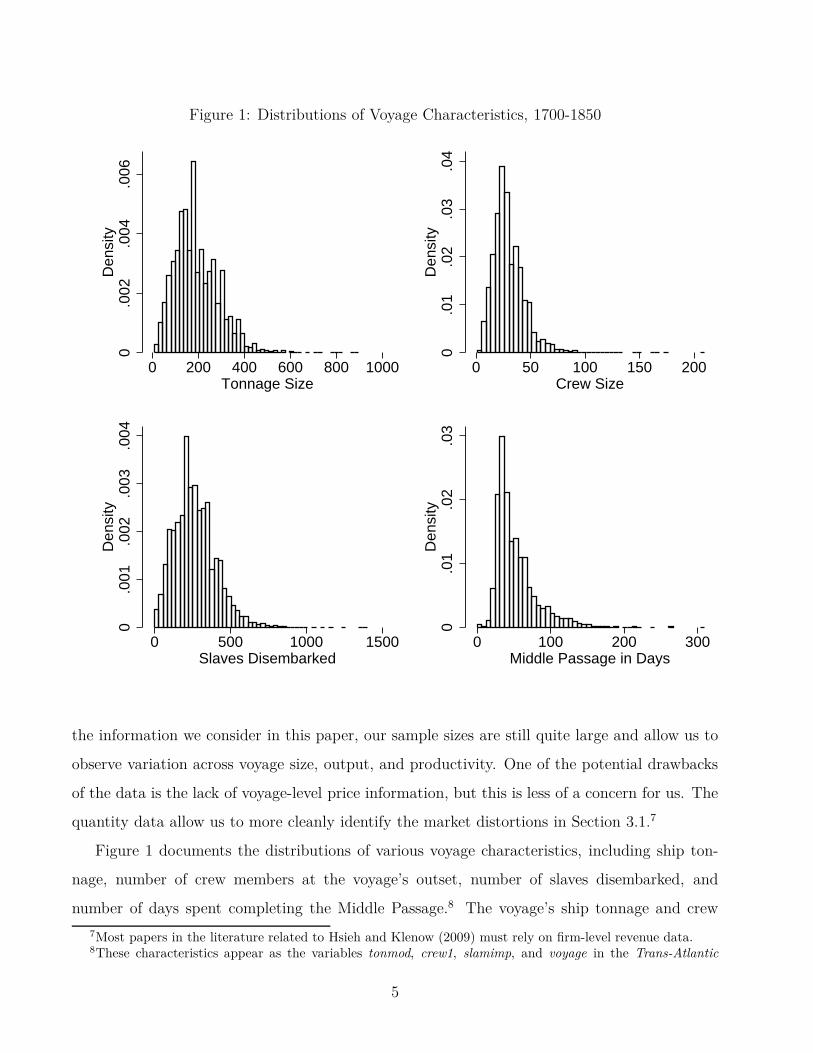
Figure 1: Distributions of Voyage Characteristics, 1700-18500

.002

.004

.006

Den

sity

0 200 400 600 800 1000Tonnage Size

0.0

1.0

2.0

3.0

4D

ensi

ty

0 50 100 150 200Crew Size

0.0

01.0

02.0

03.0

04D

ensi

ty

0 500 1000 1500Slaves Disembarked

0.0

1.0

2.0

3D

ensi

ty

0 100 200 300Middle Passage in Days

the information we consider in this paper, our sample sizes are still quite large and allow us to

observe variation across voyage size, output, and productivity. One of the potential drawbacks

of the data is the lack of voyage-level price information, but this is less of a concern for us. The

quantity data allow us to more cleanly identify the market distortions in Section 3.1.7

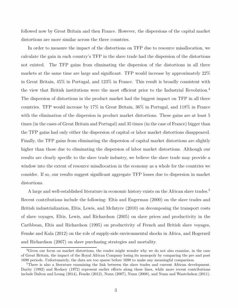
Figure 1 documents the distributions of various voyage characteristics, including ship ton-

nage, number of crew members at the voyage’s outset, number of slaves disembarked, and

number of days spent completing the Middle Passage.8 The voyage’s ship tonnage and crew

7Most papers in the literature related to Hsieh and Klenow (2009) must rely on firm-level revenue data.8These characteristics appear as the variables tonmod, crew1, slamimp, and voyage in the Trans-Atlantic

5

size correspond to capital and labor inputs, whereas slaves disembarked is a measure of voyage

output. Since not every voyage observation contains information on all four characteristics, the

number of voyage observations varies across the four distributions. Voyage-level heterogeneity

is immediately apparent, and all four distributions appear log-normal. We suppress the x-axes

of the graphs to more easily show the long and thin right tails of the distributions.9 Table 1

reports summary statistics for the four voyage characteristics.

Table 1: Summary Statistics for Voyage Characteristics, 1700-1850Mean Min Max Std. Dev. Skewness N

All VoyagesTonnage Size 194.7226 10 897.1 96.0795 0.8932 15513Crew Size 30.2323 1 210 14.9142 1.8057 11975Slaves Disembarked 267.5401 0 1400 136.6735 0.8198 29201Middle Passage in Days 52.5995 0 310 28.3594 2.0147 3735

Portugal/BrazilSlaves Disembarked 322.8620 0 1400 140.1146 0.5681 9929

Great BritainSlaves Disembarked 230.6686 0 898 103.1359 0.7774 10383

FranceSlaves Disembarked 275.3668 0 900 130.6422 0.5967 3939

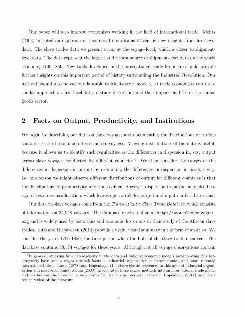
In order to address whether missing data in the Trans-Atlantic Slave Trade Database may

later bias our results, we compare observable characteristics between those voyages with complete

information and those voyages with missing information. As Table 2 suggests, there is no

statistically significant difference between the means of the characteristics across the two groups

of voyages within the three countries we are interested in (i.e. Portugal/Brazil, Great Britain

and France). Moreover, the mean composition of slaves, as measured by the percentage that are

male, does not vary significantly between the two groups and so should also not be a source of

concern.

Slave Trade Database. The countries represented by the voyages include Spain/Uruguay, Portugal/Brazil, GreatBritain, the Netherlands, the United States, France, Denmark/Baltic, and a residual category.

9Many empirical regularities in economics exhibit fat tails and follow power laws. Economists typically look atlog-log plots when analyzing these phenomena. For example, we plotted the log of voyage rank in the distributionversus the log of voyage ship tonnage. We did this for all the distributions we consider. The log-log plots showthe distributions are log-normal overall and Pareto in the tail, i.e. the tails follow a power law. Since the focusof our paper is on the heterogeneity across voyages, not the examination of the tails in particular, we do notshow the log-log plots. For an overview of power laws in economics, see Gabaix (2009).

6

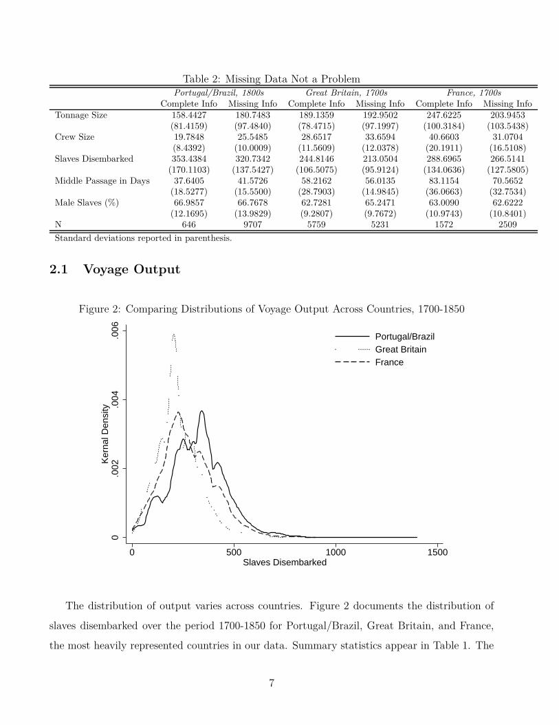
Table 2: Missing Data Not a ProblemPortugal/Brazil, 1800s Great Britain, 1700s France, 1700s

Complete Info Missing Info Complete Info Missing Info Complete Info Missing InfoTonnage Size 158.4427 180.7483 189.1359 192.9502 247.6225 203.9453

(81.4159) (97.4840) (78.4715) (97.1997) (100.3184) (103.5438)Crew Size 19.7848 25.5485 28.6517 33.6594 40.6603 31.0704

(8.4392) (10.0009) (11.5609) (12.0378) (20.1911) (16.5108)Slaves Disembarked 353.4384 320.7342 244.8146 213.0504 288.6965 266.5141

(170.1103) (137.5427) (106.5075) (95.9124) (134.0636) (127.5805)Middle Passage in Days 37.6405 41.5726 58.2162 56.0135 83.1154 70.5652

(18.5277) (15.5500) (28.7903) (14.9845) (36.0663) (32.7534)Male Slaves (%) 66.9857 66.7678 62.7281 65.2471 63.0090 62.6222

(12.1695) (13.9829) (9.2807) (9.7672) (10.9743) (10.8401)N 646 9707 5759 5231 1572 2509

Standard deviations reported in parenthesis.

2.1 Voyage Output

Figure 2: Comparing Distributions of Voyage Output Across Countries, 1700-1850

0.0

02.0

04.0

06K

erna

l Den

sity

0 500 1000 1500Slaves Disembarked

Portugal/BrazilGreat BritainFrance

The distribution of output varies across countries. Figure 2 documents the distribution of

slaves disembarked over the period 1700-1850 for Portugal/Brazil, Great Britain, and France,

the most heavily represented countries in our data. Summary statistics appear in Table 1. The

7

average number of slaves disembarked is considerably higher for Portuguese/Brazilian voyages.

Technological changes in shipping likely explain this difference, as the Portuguese/Brazilian

voyages are heavily concentrated in the 1800s. The dispersion in output is highest across Por-

tuguese/Brazilian voyages, lower across French voyages, and lowest across British voyages.

Two natural candidates come to mind when thinking about the causes of dispersion in output

within and across countries: dispersion in productive efficiency and dispersion in institutional

efficiency. Dispersion in productivity would contribute to dispersion in output. Countries also

differ by their institutions, though. Even within a country, firms face different institutional

constraints due, for instance, to political connections, which can lead to resource misallocation.

After documenting the distributions of various productivity measures across voyages in Section

2.2, we examine the role played by institutional efficiencies in Section 2.3.

2.2 Productive Efficiency

2.2.1 Four Measures of Voyage Productivity

We consider four different measures of voyage-level productivity: slaves per ton, slaves per crew,

distance, measured in kilometers, per day traveled during the Middle Passage, and TFP. The

four characteristics in Figure 1 help us to construct the productivity measures. We calculate

slaves per ton and slaves per crew directly from the data. Distance per day and TFP require

additional steps. Our construction of TFP requires a much more involved procedure, so we first

turn briefly to our distance per day measure.

The denominator of our distance per day productivity measure is taken directly from the

data presented in Figure 1.10 The distance traveled during the Middle Passage is constructed

by using GIS software. Using the geographic coordinates of a voyage’s last port of call before

making the Atlantic crossing and the first port where a voyage lands slaves, we construct the

Euclidean distance traversed during the Middle Passage.11 Our measure of distance might be

10Instead of using the distance of the Middle Passage for this measure of productivity, we could alternativelyuse the distance of the voyage’s total journey. There are not enough observations in the data including thisinformation to draw any conclusions, though. Likewise, we do not adjust our distance of the Middle Passage forseasonality. If we look at the observations with enough information to construct our distance per day measure byquarter, then the sample sizes become very small. There is not much variation in the distance per day measureby quarter, so seasonality does not appear to matter for this small number of observations.

11The variables we use for a voyage’s last and first port are npafftra and sla1port in the Trans-Atlantic Slave

8

rough, but it allows us to capture the variation of the Middle Passage across different voyages

in a simple, tractable, and commonly used way. Alternatively, great-circle distance could be

used. The trade winds used to sail across the Atlantic influenced the “distance” of the Middle

Passage, but we are unable to take into account their impact on our measure of distance.

2.2.2 TFP

In order to measure TFP, we adopt a Lucas span-of-control approach (Lucas (1978)) by assuming

the following production function for each voyage i:

Yi = (Aiφi)Kαi Lβ

i

= (Aiφi)(ηKi)αLβ

i

= AiKiαLβ

i ,

(1)

where Yi is the number of slaves disembarked in the Americas, φi is the captain’s managerial

input, Ki is capital, and Li is the number of crew, all for voyage i.12 α and β, with 0 < α+β < 1,

represent the shares of capital and labor in production, which we will assume constant across

voyages due to data constraints. Ai is unadjusted TFP. We only observe a voyage’s ship tonnage

Ki in the data, which is a proxy for the voyage’s total capital Ki. The manipulations in (1) show

how we adjust ship tonnage by the factor η and incorporate the captain’s effect to arrive at our

final production function for disembarked slaves in terms of ship tonnage, number of crew, and

TFP, Ai.13

TFP measures all those determinants of the number of slaves disembarked not captured by a

voyage’s ship tonnage and crew size, such as the quality of a voyage’s captain. Our Lucas span-

of-control approach captures the role played by a captain’s managerial ability in determining the

number of slaves disembarked. In overseeing the preparation and execution of a slave voyage,

captains performed a variety of tasks impacting the number of slaves successfully exported to

Trade Database.12We assume that slaves disembarked are homogeneous goods. In general, this is, of course, not true. For

instance, both male and female slaves were exported. But, in our data, the average proportion of male slavesexported is approximately 0.63 in all three countries studied, with a standard deviation of below 0.1. We discussthis assumption further in Section 3.1.

13We acknowledge η is not going to be constant across countries or time. Our analysis on accounting forthe TFP gain from eliminating distortions is done within a country and a decade, which should minimize thisconcern. Nevertheless, assuming η to be constant may increase the variance of voyage TFP within a country.

9

the Americas.14 Thomas (1997) writes

The captain had to be a man of parts. He was the heart and soul of the whole voyage,

and had to be able, above all, to negotiate prices of slaves with African merchants

or kings, strong enough to survive the West African climate and to stand storms,

calms, and loss of equipment. He had to have the presence of mind to deal with

difficult crews who might jump ship, and he had to be ready to face, coolly and with

courage, slave rebellions.

Thomas (1997) goes on to say French captains were required to take exams before command-

ing a slave ship. Captains often carried libraries of books on maritime techniques and ship

construction. Better knowledge of sailing would help captains deliver their cargo quicker and

lower the risk of slaves dying on board. Rawley (1981) notes captains needed to have knowledge

of the African coastline and ocean currents. Postma (1990) points out captains often oversaw

the preparations for a slave voyage, including the mix of cargo loaded in Europe to trade for

slaves on the African coast. As a result, their knowledge of demand conditions in Africa could

impact the time required to purchase and load slaves and, thus, the amount of time slaves spent

on a slave ship before departing from the African coast. Although slave ships often carried a

doctor on board to help slaves survive the Middle Passage, Rawley (1981) notes the important

role played by the captain in overseeing a ship’s hygiene. If captains understood the role of air

ventilation in fostering cleanliness, for example, it would lead to better practices on board the

ship, which would help slaves survive the journey. Captains kept the doctor on task and made

sure the doctor received any supplies required. Harms (2002) notes captains were responsible for

rationing food and water and maintaining discipline. Captains also had specialized knowledge

related to which slaves were more prone to violence and rebellion. Rawley (1981), reporting

on a Captain James Fraser, notes “...he seldom confined Angola slaves, “being very peaceable,”

took off the handcuffs of Windward and Gold Coast slaves as soon as the ship was out of sight

14A captain’s responsibilities could be made explicit in contracts. Postma (1990) reprints the contract forcaptains sailing ships for the Middelburgsche Commercie Compagnie, a Dutch slave trading company. To sum-marize the responsibilities in the contract, captains should 1) sail to the African coast as quickly as possible, 2)purchase high quality slaves, 3) not be attacked by the slaves, 4) make sure the slaves are not mistreated by thecrew, 5) make sure the slaves are treated well and taken care of by the doctor, and 6) properly brand the slavesso as not to badly injure them.

10

of land, and soon after that the leg irons, but Bonny slaves, whom he thought vicious, were

kept under stricter confinement.” Overall, a captain’s ability to manage a slave voyage played

an important role in how many slaves completed the Middle Passage.

Transforming the above production function into logarithms allows linear estimation. A

simple standard estimation equation of the production function is

ln Yi = α ln Ki + β ln Li + ǫi. (2)

The residual of the equation, ǫi, is the logarithm of TFP.

An OLS estimation of equation (2) suffers from the simultaneity problem. As Marschak and

Andrews (1944) first pointed out, part of the TFP (ǫi) might be observed by the firm before

it makes its factor input decision in that period. The regressors and the error term are, thus,

correlated, which makes the OLS estimates biased.

The bias can go either way. On the one hand, in the cross section of the voyages, better

captains (a high ǫi) will require less labor to export the same amount of slaves. These voyages

will export more with less labor. OLS will, thus, underestimate β.

On the other hand, in the time series data in which we observe the same ship over time, a

ship may get a high productivity shock (a high ǫi) and hire more labor. OLS will attribute the

increase in exports to the change in labor. OLS will overestimate β in this case.

A solution to the problem is to include ship or captain fixed effects. In our data, voyages

have information on the names of captains and ships. We use the captains’ names to identify a

unique captain. Unfortunately, there are a lot of duplications in the ships’ names, so we decide

not to include a ship fixed effect.15 The regression becomes

ln Yi = Φi + α ln Ki + β ln Li + ǫi, (3)

where Φi denotes the captain fixed effect.

15Thomas (1997) notes slave ships within a country usually had similar names. For instance, “In one list of[Portuguese] slave ships to Bahia, Nossa Senhora appeared 1,154 times, with fifty-seven different suffixes, aboveall Nossa Senhora de la Conceição (324 times); while male saints were used 1,158 times, of whom San Antônio(of Padua, but with his identity moved to Lisbon) was the most popular (695 times). Bom Jesus appeared 180times (above all, the Bom Jesus do Bom Sucesso).”

11

In addition to regressing equation (3) in which α and β are estimated separately, we also

use a second method that makes use of historical estimates on labor and capital shares in the

slave trade to estimate the production function. In particular, the production function can be

rewritten as

Yi = (Aiφi)(

K αi L1−α

i

)γ= AiφiZ

γi , (4)

where α and 1 − α represent historical estimates on capital and labor shares and γ is the so

called span-of-control parameter governing the returns to scale. The natural log of output can

be written as:

ln Yi = Φi + γ [α ln Ki + (1 − α) ln Li] + ǫi = Φi + γ ln Zi + ǫi (5)

The regression of equation (5) requires knowledge on the values for the capital and labor

shares α and 1 − α. We use the estimates reported in Eltis and Richardson (1995) to construct

separate measures for the labor share during the 1700s and 1800s. Eltis and Richardson (1995)

report values of 0.479, 0.492, and 0.532 for labor shares during the 1680s, the period 1764-1775,

and the 1780s. The values reported for the periods 1826-1835, 1836-1845, and 1856-1865 are

0.346, 0.276, and 0.242. We average the two sets of values to calculate a labor share of 0.501

for the 1700s and 0.288 for the 1800s. Since the labor share differs in the 1700s versus 1800s,

we cannot compare our measures of TFP across the two periods. This is an important point

to keep in mind, because British and French voyages occur primarily, though not exclusively,

in the 1700s, while Portuguese/Brazilian voyages are concentrated in the 1800s. From this

point forward in the paper, we only consider British and French voyages in the 1700s and

Portuguese/Brazilian voyages in the 1800s. However, the structural approach we use later to

identify the dispersion in market distortions does not rely on the labor share, and, thus, we

make comparisons between all three countries. Likewise, our main results on the TFP gains

after eliminating the dispersion in market distortions can still be compared across all three

countries.

Table 3 reports the results from different specifications of our two methods. Columns (1)

and (2) report the estimates on the capital and labor shares from equations (2) and (3), i.e.

12

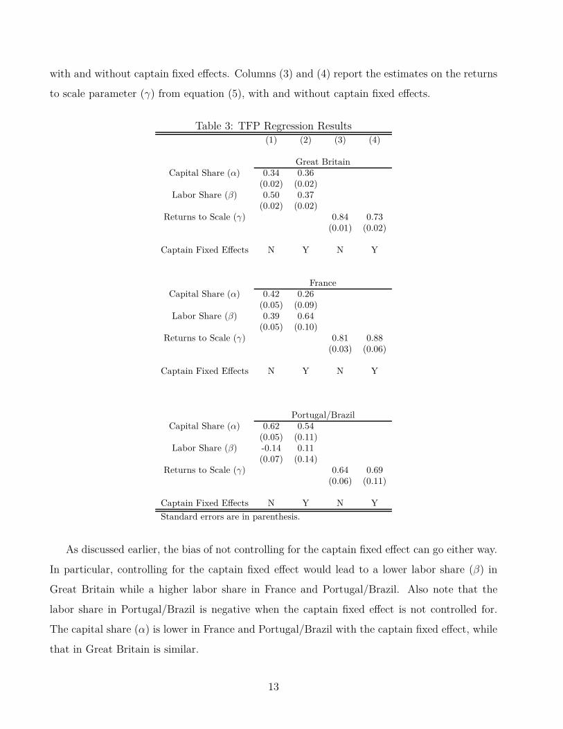
with and without captain fixed effects. Columns (3) and (4) report the estimates on the returns

to scale parameter (γ) from equation (5), with and without captain fixed effects.

Table 3: TFP Regression Results(1) (2) (3) (4)

Great BritainCapital Share (α) 0.34 0.36

(0.02) (0.02)Labor Share (β) 0.50 0.37

(0.02) (0.02)Returns to Scale (γ) 0.84 0.73

(0.01) (0.02)

Captain Fixed Effects N Y N Y

FranceCapital Share (α) 0.42 0.26

(0.05) (0.09)Labor Share (β) 0.39 0.64


(0.03) (0.06)


Portugal/BrazilCapital Share (α) 0.62 0.54

(0.05) (0.11)Labor Share (β) -0.14 0.11


(0.06) (0.11)


Standard errors are in parenthesis.

As discussed earlier, the bias of not controlling for the captain fixed effect can go either way.

In particular, controlling for the captain fixed effect would lead to a lower labor share (β) in

Great Britain while a higher labor share in France and Portugal/Brazil. Also note that the

labor share in Portugal/Brazil is negative when the captain fixed effect is not controlled for.

The capital share (α) is lower in France and Portugal/Brazil with the captain fixed effect, while

that in Great Britain is similar.

13

The two specifications from equations (3) and (5) also yield similar capital and labor shares

in Great Britain and Portugal/Brazil. When estimated separately (column 2), the capital shares

in Great Britain and in Portugal/Brazil are 0.36 and 0.54, and they are 0.36 (0.73 × 0.499) and

0.49 (0.69×0.712) when the ratio of the capital share to the labor share is restricted to historical

averages. Similarly, the estimates of labor shares are 0.37 in both specifications in Great Britain.

The estimates of Portuguese/Brazilian labor shares are 0.11 and 0.20 (0.69 × 0.288), but the

difference is not statistically significant. The labor and capital share estimates for French voyages

are different across the two specifications. When estimated separately, the labor share estimate

is higher than the historical average, and the capital share estimate is lower than the historical

average.

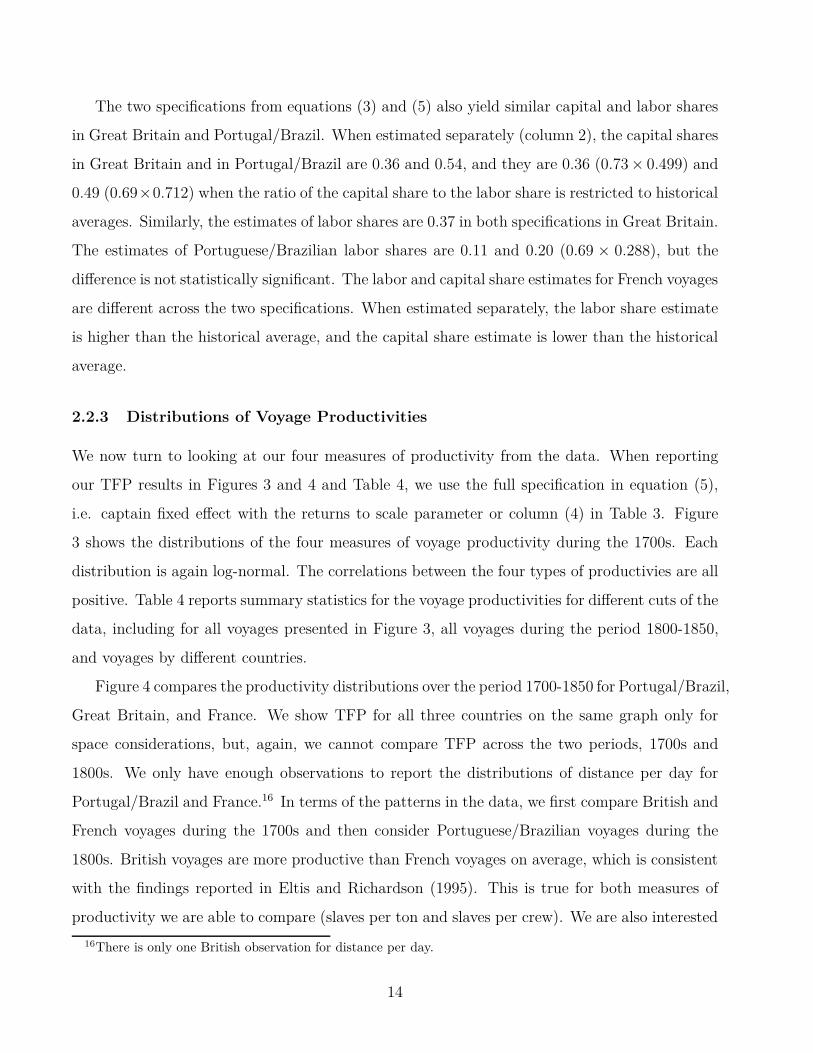
2.2.3 Distributions of Voyage Productivities

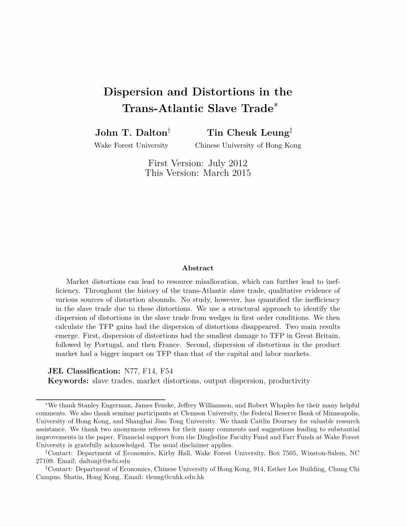
We now turn to looking at our four measures of productivity from the data. When reporting

our TFP results in Figures 3 and 4 and Table 4, we use the full specification in equation (5),

i.e. captain fixed effect with the returns to scale parameter or column (4) in Table 3. Figure

3 shows the distributions of the four measures of voyage productivity during the 1700s. Each

distribution is again log-normal. The correlations between the four types of productivies are all

positive. Table 4 reports summary statistics for the voyage productivities for different cuts of the

data, including for all voyages presented in Figure 3, all voyages during the period 1800-1850,

and voyages by different countries.

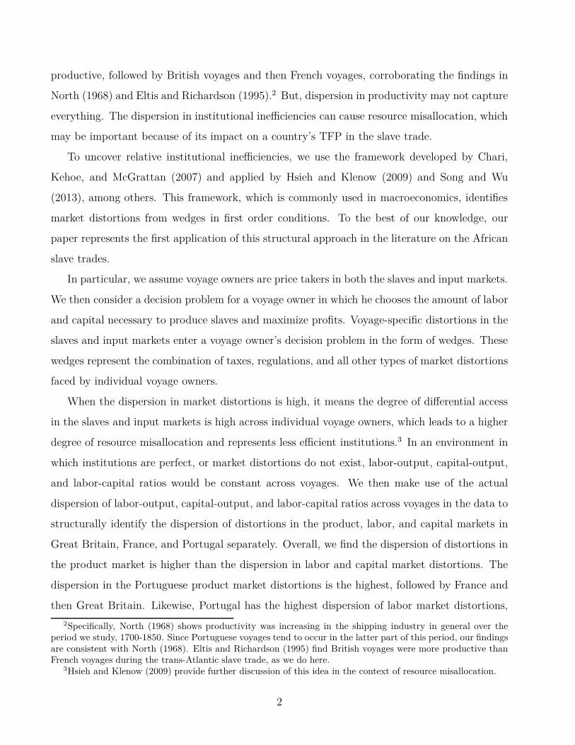
Figure 4 compares the productivity distributions over the period 1700-1850 for Portugal/Brazil,

Great Britain, and France. We show TFP for all three countries on the same graph only for

space considerations, but, again, we cannot compare TFP across the two periods, 1700s and

1800s. We only have enough observations to report the distributions of distance per day for

Portugal/Brazil and France.16 In terms of the patterns in the data, we first compare British and

French voyages during the 1700s and then consider Portuguese/Brazilian voyages during the

1800s. British voyages are more productive than French voyages on average, which is consistent

with the findings reported in Eltis and Richardson (1995). This is true for both measures of

productivity we are able to compare (slaves per ton and slaves per crew). We are also interested

16There is only one British observation for distance per day.

14

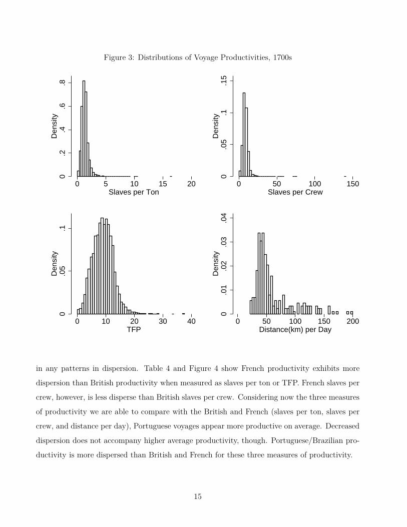
Figure 3: Distributions of Voyage Productivities, 1700s0

.2.4

.6.8

Den

sity

0 5 10 15 20Slaves per Ton

0.0

5.1

.15

Den

sity

0 50 100 150Slaves per Crew

0.0

5.1

Den

sity

0 10 20 30 40TFP

0.0

1.0

2.0

3.0

4D

ensi

ty

0 50 100 150 200Distance(km) per Day

in any patterns in dispersion. Table 4 and Figure 4 show French productivity exhibits more

dispersion than British productivity when measured as slaves per ton or TFP. French slaves per

crew, however, is less disperse than British slaves per crew. Considering now the three measures

of productivity we are able to compare with the British and French (slaves per ton, slaves per

crew, and distance per day), Portuguese voyages appear more productive on average. Decreased

dispersion does not accompany higher average productivity, though. Portuguese/Brazilian pro-

ductivity is more dispersed than British and French for these three measures of productivity.

15

Table 4: Summary Statistics for Voyage Productivities, 1700-1850Mean Min Max Std. Dev. Skewness N

All Voyages, 1700sSlaves per Ton 1.3408 0 16.6063 0.6929 3.9791 10927Slaves per Crew 8.7250 0 141.4500 4.3210 6.7879 8461Distance(km) per Day 59.7129 21.1417 199.5254 33.8018 1.7735 248

All Voyages, 1800sSlaves per Ton 1.8355 0.0042 17.3306 1.2425 3.2407 3377Slaves per Crew 13.7272 0.0426 95 9.7955 2.4281 2710Distance(km) per Day 120.6148 46.3681 239.4305 42.6388 0.5825 69

Portugal/Brazil, 1800sSlaves per Ton 2.5243 0.0042 17.3306 1.4473 3.5938 1105Slaves per Crew 17.5295 0.0667 95 10.8061 1.9586 1247TFP 17.2550 0.0497 62.3145 7.4214 0.9772 646Distance(km) per Day 120.7905 46.3681 239.4305 42.3295 0.6199 67

Great Britain, 1700sSlaves per Ton 1.3949 0 10.4250 0.6387 3.2202 7781Slaves per Crew 9.0546 0 141.4500 4.3938 8.1904 5803TFP 9.9895 0.1609 37.6443 3.1666 0.6648 5759

France, 1700sSlaves per Ton 1.2299 0 16.6063 0.7743 6.2570 2188Slaves per Crew 7.8475 0 44.2833 3.7042 2.7695 2156TFP 5.3771 0.0345 33.7378 2.4184 2.5936 1572Distance(km) per Day 45.7658 21.1417 141.4387 14.9083 2.6161 195

16

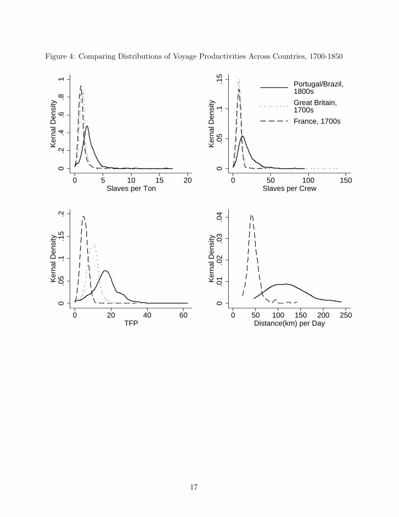
Figure 4: Comparing Distributions of Voyage Productivities Across Countries, 1700-18500

.2.4

.6.8

1K

erna

l Den

sity

0 5 10 15 20Slaves per Ton

0.0

5.1

.15

Ker

nal D

ensi

ty

0 50 100 150Slaves per Crew

Portugal/Brazil,1800s

Great Britain,1700s

France, 1700s

0.0

5.1

.15

.2K

erna

l Den

sity

0 20 40 60TFP

0.0

1.0

2.0

3.0

4K

erna

l Den

sity

0 50 100 150 200 250Distance(km) per Day

17

2.3 Institutional Efficiency

Not only did productive efficiency (i.e. TFP) vary across and within different countries between

1700 and 1850, there was also substantial variation in institutional efficiency, which impacted

the workings of the factor (i.e. labor and capital) and product (i.e. slaves) markets. Much

of the period of the slave trades can be characterized by well-documented mercantilist policies

imposed by various European states and their associated inefficiencies. Eltis and Richardson

(1995) make this same point. In these types of economies, firms with close connections to royal

families would be in more advantageous positions than firms without such connections. Pearson

and Richardson (2001) emphasize the importance of these networks and the differential access

they afford during the period we study.17 The degree of the mercantilist policies varied across

the countries we study. For instance, the Royal African Company lost its monopoly over the

English slave trade in 1698, while the royal families in France and Portugal still had a lot of

influence on the slave trade throughout the 1700s. French slave trading was characterized by

an elaborate subsidy system known as the Acquits de Guinée, and the Compagnie du Sénégal

maintained monopoly rights over exporting slaves from Senegambia. Thomas (1997) goes so far

as to assert “the prime mover in the slaving business was the state.”

Inefficiencies in the factor and product markets of the slave trades, which we document

below, gave rise to variation in the prices of slaves. For example, the slave prices in non-British

colonies were higher than that in the British colonies in the 1700s, as mentioned in a letter cited

in Inikori (1981) from John Tarleton to his brother and partner in 1790:

Since I wrote you last, I have seen Mr. H. Le Mesurier, who set out in the Mail last

night for Liverpool, and had a long conversation with him respecting his scheme for

our future adventures to St. Domingo, as a joint concern with the house at Havre;

which from the continuance of the French bounties, and an uncommon demand for

negroes, would, I am persuaded, turn out a most lucrative one, and far superior in

every respect to what we can possibly expect in any of the English Islands, where

the risk of bad debts is nearly equal with what it is in the French Islands, with only

two-thirds of the price for each slave.

17In a different context well-known to economic historians, Greif (1989) and Greif (1993) describe the importantrole played by reputation in smoothing international transactions.

18

Eltis and Richardson (2004) also document substantial slave price variations across different

ports in the New World. In their paper, they show that Jamaica and St. Domingue, which are

close geographically, had different slave prices in the eighteenth century.

Thomas (1997) documents the many different state policies giving rise to product market

distortions in the slave trades. During the time when the Royal African Company had its

privilege over the British slave trade, independent traders paid an ad valorem tax to the company

to engage in the trade. In the case of the Portuguese, slave traders were supposed to stop in the

Cape Verde Islands to pay duties. Two state companies, the Maranhao created in 1755 and the

Pernambuco created in 1759, were exempt from the export taxes paid by their competitors. In

France, any merchant could engage in the slave trades, provided they sail from one of the five

privileged ports of Rouen, La Rochelle, Bordeaux, Saint-Malo, and Nantes. French slave traders

then paid a tax per slave to sell their product, which varied based on the French colony in which

the sale was made. Taxes were not only levied by the European side of the colonial system

but also by colonial assemblies themselves. Thomas (1997) mentions the Jamaican Assembly’s

imposition of a local tax on slaves exported from Jamaica, including those being transshipped.

The levels of distortions firms faced at the time were highly asymmetric due to differential

access in the product market. Thomas (1997) notes slave traders bought plantations in the

New World to help establish networks for purchasing slaves. The networks of purchasing agents

often included family members of slave traders. British access to non-British colonies serves as

another example. It was either by special license from the European governments in charge or

by underground arrangements. These set a high entry barrier which favored the large firms that

had connections. In 1789, John Dawson, the largest supplier of slaves to non-British colonies

at the time, told a committee of the Privy Council that he signed a special contract with the

Spanish government and had landed 12,000 slaves in the Spanish colonies between 1785 and

1788. Procurement of slaves from the African coast could also contribute to product market

inefficiencies. Eltis and Richardson (1995) note the French crown granted monopoly rights over

exporting slaves from Senegambia for much of the 1700s to one firm, the Compagnie du Sénégal.

Rival French traders were forced further south down the African coast to find alternative sources

of slaves. As Harms (2002) points out, even though much of the slave trade began to open up

to private traders during the 1700s, the former monopoly companies still retained ownership

19

of important trading forts and castles along the African coast and, thus, maintained strategic

access to slave markets in Africa.

The European labor market in the 1700s and 1800s was highly inefficient. One indication of

labor market inefficiency is wage dispersion. Historical wage dispersion across European cities, as

well as within a European country such as Great Britain and France, has been well documented.

Allen (2001), making use of the wage and grain price data made available by Phelps Brown and

Hopkins (1981), shows that wage dispersion existed in Europe in the 1700s. Williamson (1995)

and Williamson (1996) document substantial wage dispersion among the OECD members in the

1800s. Hunt (1973), Pollard (1959), and Sicsic (1992) provide evidence of the wide wage gaps

between the urban and rural areas in Great Britain and France in the 1800s.

The labor markets upon which slave traders depended were no exception. Eltis and Richard-

son (1995) cites the Five Great Farms, the internal French customs union, as an example of an

institutional constraint on the equalization of costs across French ports. Rawley (1981) claims

that Liverpool merchants “paid lower wages to seamen and captains and lower commission to

factors than did merchants in other ports.” According to Thomas (1997), this was “one reason

why the former (Liverpool merchants) were able to sell their cargoes for 12 percent less than

the rest of the kingdom, and return with an equal profit.” In some cases, crew members were

secured through crimping, and voyage owners presumably varied in their ability and willingness

to crimp. Thomas (1997) describes the practice by relating the following:

A carpenter in the navy, James Towne, told a House of Commons committee on the

slave trade: “The method at Liverpool [to obtain sailors] is by the merchants’ clerks

going from public house to public house, giving them liquors to get them into a state

of intoxication and, by that, getting them very often on board. Another method is

to get them in debt and then, if they don’t choose to go aboard of such guinea men

then ready for sea, they are sent away to gaol by the publicans they may be indebted

to.”

The extent of the development of the credit markets servicing the slave trades varied across

European ports, and access to the best markets would be an advantage to a slave trading firm.

The case of Liverpool’s prominence, for example, is well known. Rawley (1981) provides a

20

thorough discussion of the advantages connections to Liverpool provided. Capital expenditures

for a voyage were often shared by small groups of investors. Thomas (1997) notes, “The most

frequent type of association . . . was one of relations, the only tie which could be trusted to

endure.” As a result, families came to dominate the financing of the slave trades to a large

extent. Viles (1972) notes the slave traders of Bordeaux and La Rochelle were a minority group

of Protestant merchants with close family ties. These Protestant slavers only exerted influence

on the commercial institutions of their city in La Rochelle, not Roman Catholic controlled

Bordeaux. The financiers themselves often had access to pools of capital through their many

commercial interests.

The mercantile policies in different European states created additional capital market distor-

tions. Rawley (1981) describes the French subsidy system, which included a bounty per ton for

ships. Rawley (1981) notes the effect of the distortion: “The bounty for tonnage, intended to

encourage use of larger ships, had the unhappy result of encouraging fraud. Ships miraculously

doubled in size.”

Small firms were also disadvantaged in the credit market such that they might have to pay

a premium to secure labor services. A letter mentioned in Inikori (1981) from Joseph Canton,

one of the small slave traders in Liverpool, to James Rogers, who owned a badly managed slave

trade firm which went bankrupt in the 1790s indicated the importance of connections in the

local credit market:

When you sent me that Bill of £500 I put it into Mr. Heywood’s Bank with that

intent to take cash as occasion required. Mr. Heywood sent this bill up to Mr.

Joseph Denison in London, their Banking house, to enquire into the utility of the

Bill. Mr. Denison in his usual way as he often does sends this bill down again and

says the Bill may be good but he knows nothing of the acceptor or Drawer and such

bills is out of his way. So Heywood has sent it to me which I have by now.

Inikori (1981) argues the more limited access to credit markets also affected the levels of muni-

tions and insurance available to small firms. Donnan (1930) documents a marine insurer from

London explaining to a slave trader from Newport, Rhode Island that “the premium for a winter

voyage from Jamaica is never less than 8 percent and upon vessels not known in the trade can

21

seldom be under 10.” According to Thomas (1997), insurance rates varied from 5% to 25%. Price

and Clemens (1987) find the same pattern of small firms disadvantaged in credit and insurance

markets during the same time period as the slave trades but for a different trade, namely, the

Chesapeake trade plied by British firms.

3 Accounting for TFP Loss Due to Dipersion

3.1 A Structural Model for Measuring Distortions

Our method for analyzing the data resembles the business cycle accounting framework developed

by Chari, Kehoe, and McGrattan (2007) and applied by Hsieh and Klenow (2009) and Song and

Wu (2013), among many others.18 The procedure relies on a structural model of the economy

and infers the distortions in the input and output markets from the residuals, or wedges, in the

first order conditions. For example, when used in examining the sources of the fluctuations in a

series of GDP per capita, this approach allows the researcher to identify the relevant distortions,

information which can then be used to think about the details and underlying mechanisms

generating the fluctuations. The procedure can also be applied under various market structures

and different types of models. Chari, Kehoe, and McGrattan (2007) base the discussion around

a perfectly competitive environment but established equivalency results for a large class of

models, whereas Hsieh and Klenow (2009) consider a monopolistically competitive environment

à la Melitz (2003).

In order to examine the product, labor, and capital market distortions during the slave

trades, we consider a simple decision problem where a firm, or a voyage, hires labor and invests

in capital to produce output, slaves disembarked. Each voyage has access to the decreasing

returns to scale production function shown in equation (1) and makes decisions in a competitive

environment where prices, wages, and rental rates are given. Voyages differ by their TFP and

the distortions they face in the output and input markets. Lastly, the slaves disembarked are

homogeneous products. While slaves differed by age, gender, quality, etc., the data do not permit

18The term business cycle accounting originates with the application to business cycles in Chari, Kehoe, andMcGrattan (2007), but their method can be extended to many other applications, including the distribution ofresources as done by Hsieh and Klenow (2009).

22

us to identify this variation. Also, newly arrived slaves may have been largely undifferentiated

from the perspective of the buyer, because characteristics, such as field productivity and life

expectancy, were difficult to measure before being tested by life in the Americas. Eltis, Lewis,

and Richardson (2005) make this same point when assuming slaves were largely homogeneous

products. We now can turn to the voyage decision problem.

For a given productive capital stock Ki, voyage i chooses Yi and Li to maximize profits

subject to its production function

maxYi,Li

(1 − τpi )pYi − (1 + τw

i )wLi s.t. Yi = AiKαi Lβ

i (6)

where p is the price received for a slave in the Americas and w is the wage rate paid to a voyage

crew member. τ pi and τw

i represent the distortions in the product market and labor market faced

by an individual voyage i. Solving the voyage problem yields the following expressions:

Li =βΦiK

α/1−βi

(1 + τwi )w

Yi =ΦiK

α/1−βi

(1 − τpi )p

πi = (1 − β)ΦiKi

α/1−β,

where πi represents voyage i’s profits and Φi =(

ββAi(1−τp

i)p

[(1+τwi

)w]β

)1/1−β

.

We also model the distortions in the capital market. In particular, we use τ ri to summarize

the effects of capital market distortions on the capital goods price that voyage i faces:

Ri = (1 + τ ri )R, (7)

where R is the average capital goods price.

The law of motion for capital is as follows. Voyage i has an initial amount of capital, Ki,

at the beginning of each period. It can purchase new investment, Ii, which contributes to the

productive capital, Ki. The capital will depreciate by the portion δ in the next period, which

23

then determines K ′

i. The law of motion for capital is then

K ′

i = (1 − δ)Ki = (1 − δ)(Ki + Ii). (8)

The investment problem for voyage i is defined by the Bellman equation:

V (Φi, Ki) = maxIi

{

π(Φi, Ki, Ii) − RiIi +V (Φi, K ′

i)

1 + r

}

, (9)

where 1/1 + r is the discount factor. Define J as the Jorgensonian user cost of capital:

J ≡ R

(

1 −1 − δ

1 + r

)

. (10)

Following Bloom (2009) and Song and Wu (2013), our timing assumption on investment allows

for a closed form solution for investment, because it is straightforward to show, by guess and

verify, that the value function is linear in Ki:

V (Φi, Ki) = RiKi + C, (11)

where C is a constant in Ki. The productive capital is then as follows:

Ki =

[

Φiα

(1 + τ ri )J

]1−β

1−α−β

. (12)

The input-output ratios and labor-capital ratio are then:

Li

Yi= β

(1 − τpi )p

(1 + τwi )w

(13)

Ki

Yi

= α(1 − τp

i )p

(1 + τ ri )J

(14)

Li

Ki

=β

α

(1 + τ ri )J

(1 + τwi )w

. (15)

We assume the log of the distortions is distributed normally with zero mean and that the

distributions are independent. Song and Wu (2013) have a similar assumption on the labor and

capital market distortions in China. The variances of the log of the ratios in equations (13) to

24

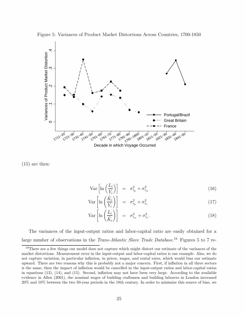
Figure 5: Variances of Product Market Distortions Across Countries, 1700-1850

0.1

.2.3

.4V

aria

nces

of P

rodu

ct M

arke

t Dis

tort

ion

1711−20

1721−30

1731−40

1741−50

1751−60

1761−70

1771−80

1781−90

1791−1800

1801−10

1811−20

1821−30

1831−40

1841−50

Decade in which Voyage Occurred


(15) are then:

Var[

ln(

Li

Yi

)]

= σ2τp

+ σ2τw

(16)

Var

[

ln

(

Ki

Yi

)]

= σ2τp

+ σ2τr

(17)

Var

[

ln

(

Li

Ki

)]

= σ2τw

+ σ2τr

. (18)

The variances of the input-output ratios and labor-capital ratio are easily obtained for a

large number of observations in the Trans-Atlantic Slave Trade Database.19 Figures 5 to 7 re-

19There are a few things our model does not capture which might distort our estimate of the variances of themarket distortions. Measurement error in the input-output and labor-capital ratios is one example. Also, we donot capture variation, in particular inflation, in prices, wages, and rental rates, which would bias our estimateupward. There are two reasons why this is probably not a major concern. First, if inflation in all three sectorsis the same, then the impact of inflation would be cancelled in the input-output ratios and labor-capital ratiosin equations (13), (14), and (15). Second, inflation may not have been very large. According to the availableevidence in Allen (2001), the nominal wages of building craftsmen and building laborers in London increased20% and 10% between the two 50-year periods in the 18th century. In order to minimize this source of bias, we

25

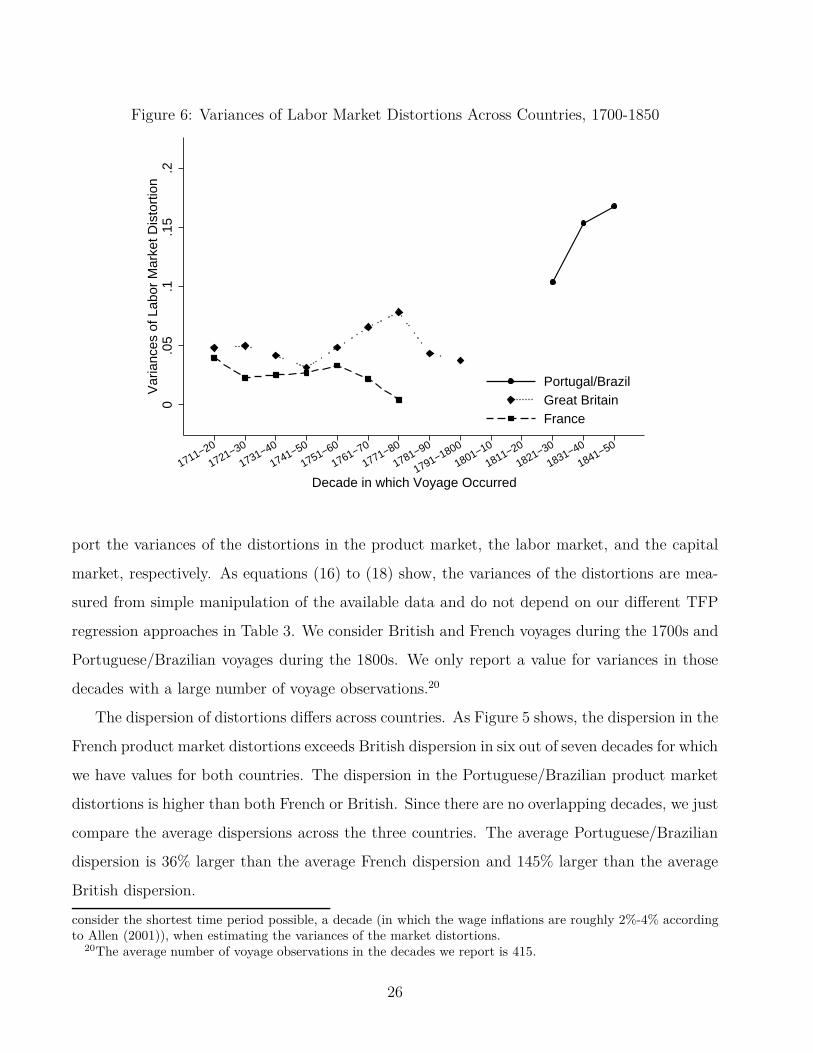
Figure 6: Variances of Labor Market Distortions Across Countries, 1700-1850

0.0

5.1

.15

.2V

aria

nces

of L

abor

Mar

ket D

isto

rtio

n

1711−20

1721−30

1731−40

1741−50

1751−60

1761−70

1771−80

1781−90

1791−1800

1801−10

1811−20

1821−30

1831−40

1841−50



port the variances of the distortions in the product market, the labor market, and the capital

market, respectively. As equations (16) to (18) show, the variances of the distortions are mea-

sured from simple manipulation of the available data and do not depend on our different TFP

regression approaches in Table 3. We consider British and French voyages during the 1700s and

Portuguese/Brazilian voyages during the 1800s. We only report a value for variances in those

decades with a large number of voyage observations.20

The dispersion of distortions differs across countries. As Figure 5 shows, the dispersion in the

French product market distortions exceeds British dispersion in six out of seven decades for which

we have values for both countries. The dispersion in the Portuguese/Brazilian product market

distortions is higher than both French or British. Since there are no overlapping decades, we just

compare the average dispersions across the three countries. The average Portuguese/Brazilian

dispersion is 36% larger than the average French dispersion and 145% larger than the average

British dispersion.

consider the shortest time period possible, a decade (in which the wage inflations are roughly 2%-4% accordingto Allen (2001)), when estimating the variances of the market distortions.

20The average number of voyage observations in the decades we report is 415.

26

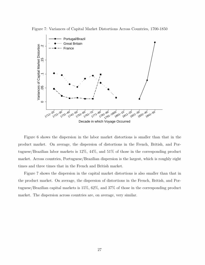
Figure 7: Variances of Capital Market Distortions Across Countries, 1700-1850

0.0

5.1

.15

.2V

aria

nces

of C

apita

l Mar

ket D

isto

rtio

n

1711−20

1721−30

1731−40

1741−50

1751−60

1761−70

1771−80

1781−90

1791−1800

1801−10

1811−20

1821−30

1831−40

1841−50



Figure 6 shows the dispersion in the labor market distortions is smaller than that in the

product market. On average, the dispersion of distortions in the French, British, and Por-

tuguese/Brazilian labor markets is 12%, 44%, and 51% of those in the corresponding product

market. Across countries, Portuguese/Brazilian dispersion is the largest, which is roughly eight

times and three times that in the French and British market.

Figure 7 shows the dispersion in the capital market distortions is also smaller than that in

the product market. On average, the dispersion of distortions in the French, British, and Por-

tuguese/Brazilian capital markets is 15%, 62%, and 37% of those in the corresponding product

market. The dispersion across countries are, on average, very similar.

27

3.2 Contribution of Institutional Efficiency to TFP

Backing out the variances is important in understanding the impact of distortions on the coun-

try’s TFP in the slave trade. The country’s TFP in the slave trade is:

TFP =

∑

i Yi

(∑

i Ki)α(∑

i Li)β. (19)

Our measure of the country’s TFP in the slave trade is similar to the industry measure of TFP

in Hsieh and Klenow (2009).

If Ai, (1 − τpi ), (1 + τ r

i ), and (1 + τwi ) are jointly but independently lognormal distributed,

the aggregate output, aggregate labor, and aggregate capital can be shown as

∑

i

Yi ≈

[

pα+βααββ

Jαwβ

]1/1−α−β

N exp

[

A

1 − α − β+

σ2A

+ (α + β)2σ2τp

+ α2σ2τr

+ β2σ2τw

2(1 − α − β)2

]

(20)

∑

i

Li ≈

[

pααβ1−α

Jαw1−α

]1/1−α−β

N exp

[

A

1 − α − β+

σ2A

+ σ2τp

+ α2σ2τr

+ (1 − α)2σ2τw

2(1 − α − β)2

]

(21)

∑

i

Ki ≈

[

pα1−βββ

J1−βwβ

]1/1−α−β

N exp

[

A

1 − α − β+

σ2A

+ σ2τp

+ (1 − β)2σ2τr

+ β2σ2τw

2(1 − α − β)2

]

, (22)

where A is the mean of ln Ai and N is the number of voyages.21 Substituting equations (20)

to (22) into equation (19), we can express the natural log of the country’s TFP as a decreasing

function of the variances of the distortions:

ln TFP = A + (1 − α − β) ln N +σ2

A− (α + β)σ2

τp− α(1 − β)σ2

τr− β(1 − α)σ2

τw

2(1 − α − β). (23)

Just like in Hsieh and Klenow (2009), dispersion in distortions worsens misallocation, because

it generates higher dispersion in marginal products.

Tables 5 and 6 report the TFP gain for the three countries when the variances of distortions

disappear. Table 5 shows results using the specification with the returns to scale parameter

21The appendix provides details for deriving equations (20) - (22). We also show in the appendix how allowingthe distortions to be correlated affects our results.

28

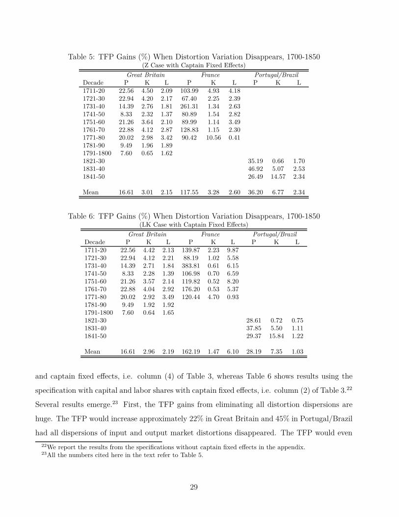
Table 5: TFP Gains (%) When Distortion Variation Disappears, 1700-1850(Z Case with Captain Fixed Effects)

Great Britain France Portugal/BrazilDecade P K L P K L P K L1711-20 22.56 4.50 2.09 103.99 4.93 4.181721-30 22.94 4.20 2.17 67.40 2.25 2.391731-40 14.39 2.76 1.81 261.31 1.34 2.631741-50 8.33 2.32 1.37 80.89 1.54 2.821751-60 21.26 3.64 2.10 89.99 1.14 3.491761-70 22.88 4.12 2.87 128.83 1.15 2.301771-80 20.02 2.98 3.42 90.42 10.56 0.411781-90 9.49 1.96 1.891791-1800 7.60 0.65 1.621821-30 35.19 0.66 1.701831-40 46.92 5.07 2.531841-50 26.49 14.57 2.34

Mean 16.61 3.01 2.15 117.55 3.28 2.60 36.20 6.77 2.34

Table 6: TFP Gains (%) When Distortion Variation Disappears, 1700-1850(LK Case with Captain Fixed Effects)


Mean 16.61 2.96 2.19 162.19 1.47 6.10 28.19 7.35 1.03

and captain fixed effects, i.e. column (4) of Table 3, whereas Table 6 shows results using the

specification with capital and labor shares with captain fixed effects, i.e. column (2) of Table 3.22

Several results emerge.23 First, the TFP gains from eliminating all distortion dispersions are

huge. The TFP would increase approximately 22% in Great Britain and 45% in Portugal/Brazil

had all dispersions of input and output market distortions disappeared. The TFP would even

22We report the results from the specifications without captain fixed effects in the appendix.23All the numbers cited here in the text refer to Table 5.

29

more than double (123%) in France had these dispersions disappeared.

Second, the dispersion of distortions in the product market had the largest impact on a

country’s TFP for all three countries in our study. TFP would increase 17% in Great Britain,

118% in France, and 36% in Portugal/Brazil had the dispersion of the product market distortions

disappeared. These gains are at least 5 times (in Great Britain and Portugal/Brazil) and 35

times (in France) bigger than the TFP gains had only either the dispersion of capital or labor

market distortions disappeared.

Third, the TFP losses due to capital market distortions, while much smaller than that due

to product market distortions, are slightly higher than that due to labor market distortions. In

Great Britain, TFP loss due to capital market distortion dispersion is on average 3%, while the

TFP loss due to labor market distortion dispersion is on average 2%. In France, the TFP losses

from capital and labor market distortion dispersion are similar. In Portugal/Brazil, the TFP

loss due to capital market distortion dispersion is even higher at almost 7%, while the TFP loss

due to labor market distortion dispersion is slightly higher than 2%.

4 Conclusion

The slave trading economy of the Atlantic was characterized by numerous distortions in output

and input markets. These distortions gave rise to resource misallocation, which then impacted

TFP in the slave trades. This paper is the first to quantify the inefficiency in the slave trades

of Great Britain, France, and Portugal due to market distortions. We structurally identify

the dispersion of the distortions in the output and input markets from wedges in first order

conditions. Our procedure should prove useful as a diagnostic tool for economic historians

working on a range of topics. Market distortions played a significant role in depressing TFP

in the slave trades. Eliminating all the dispersion of the distortions in the output and input

markets would have increased TFP by 22% in Great Britain, 45% in Portugal, and 123% in

France. The dispersion of the distortions in the product markets had the biggest impact on

TFP.

Our findings shed new light on the industrial structure of the Atlantic economy during the

time of the slave trades. Although historians and economic historians have made great strides

30

in documenting and analyzing the slave trades, there is still room for further research, especially

given the wealth of firm-level data during this historical period. Future research should exploit

the richness of the data, as we have tried to do in this paper.

31

A Appendix

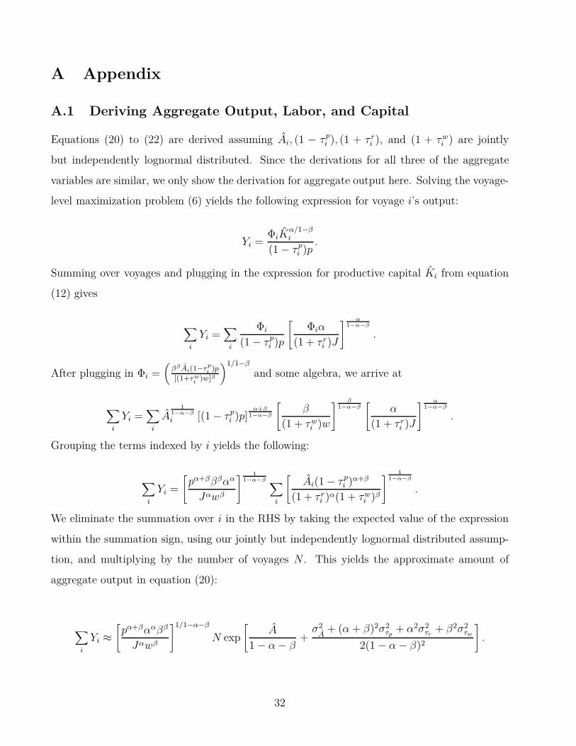
A.1 Deriving Aggregate Output, Labor, and Capital

Equations (20) to (22) are derived assuming Ai, (1 − τpi ), (1 + τ r

i ), and (1 + τwi ) are jointly

but independently lognormal distributed. Since the derivations for all three of the aggregate

variables are similar, we only show the derivation for aggregate output here. Solving the voyage-

level maximization problem (6) yields the following expression for voyage i’s output:

Yi =ΦiK

α/1−βi

(1 − τpi )p

.

Summing over voyages and plugging in the expression for productive capital Ki from equation

(12) gives

∑

i

Yi =∑

i

Φi

(1 − τpi )p

[

Φiα

(1 + τ ri )J

] α1−α−β

.

After plugging in Φi =(

ββAi(1−τp

i)p

[(1+τwi

)w]β

)1/1−β

and some algebra, we arrive at

∑

i

Yi =∑

i

A1

1−α−β

i [(1 − τpi )p]

α+β

1−α−β

[

β

(1 + τwi )w

]β

1−α−β[

α

(1 + τ ri )J

] α1−α−β

.

Grouping the terms indexed by i yields the following:

∑

i

Yi =

[

pα+βββαα

Jαwβ

] 1

1−α−β∑

i

[

Ai(1 − τpi )α+β

(1 + τ ri )α(1 + τw

i )β

]

1

1−α−β

.

We eliminate the summation over i in the RHS by taking the expected value of the expression

within the summation sign, using our jointly but independently lognormal distributed assump-

tion, and multiplying by the number of voyages N . This yields the approximate amount of

aggregate output in equation (20):

∑

i

Yi ≈

[

pα+βααββ

Jαwβ

]1/1−α−β

N exp

[

A

1 − α − β+

σ2A

+ (α + β)2σ2τp

+ α2σ2τr

+ β2σ2τw

2(1 − α − β)2

]

.

32

where A is the mean of ln Ai.

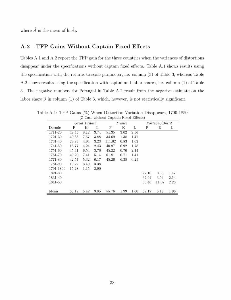
A.2 TFP Gains Without Captain Fixed Effects

Tables A.1 and A.2 report the TFP gain for the three countries when the variances of distortions

disappear under the specifications without captain fixed effects. Table A.1 shows results using

the specification with the returns to scale parameter, i.e. column (3) of Table 3, whereas Table

A.2 shows results using the specification with capital and labor shares, i.e. column (1) of Table

3. The negative numbers for Portugal in Table A.2 result from the negative estimate on the

labor share β in column (1) of Table 3, which, however, is not statistically significant.

Table A.1: TFP Gains (%) When Distortion Variation Disappears, 1700-1850(Z Case without Captain Fixed Effects)


Mean 35.12 5.42 3.85 55.76 1.99 1.60 32.17 5.18 1.96

33

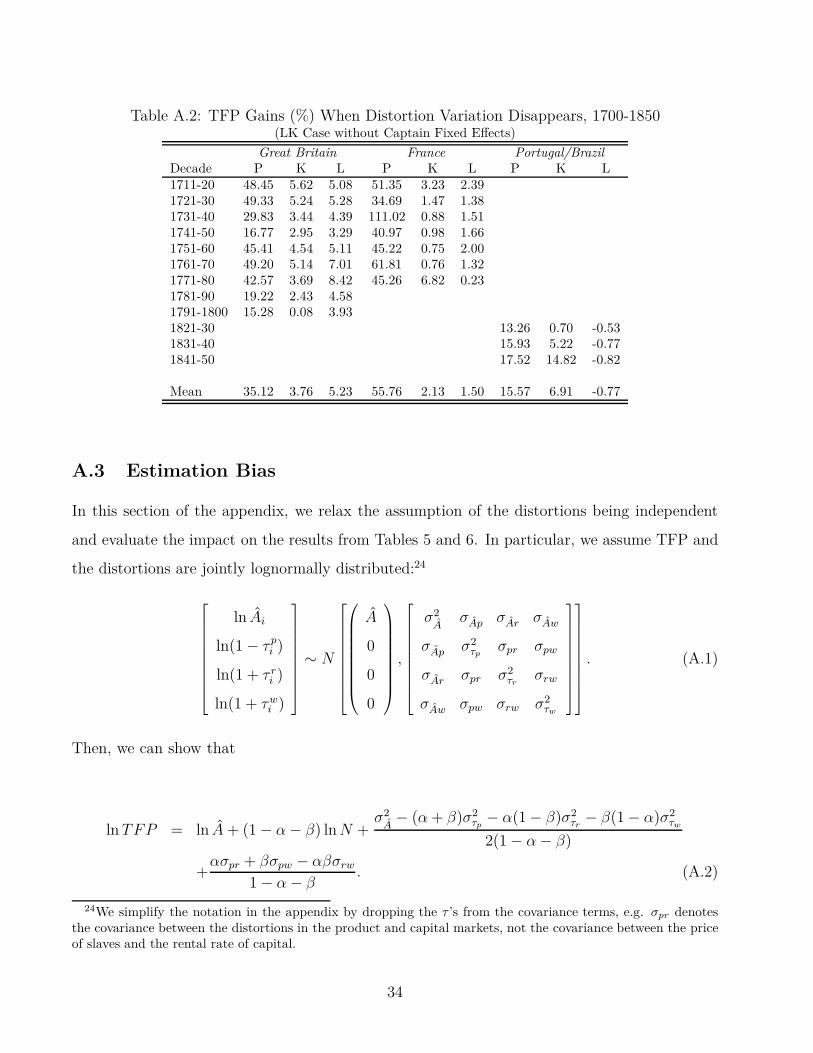
Table A.2: TFP Gains (%) When Distortion Variation Disappears, 1700-1850(LK Case without Captain Fixed Effects)

Great Britain France Portugal/BrazilDecade P K L P K L P K L1711-20 48.45 5.62 5.08 51.35 3.23 2.391721-30 49.33 5.24 5.28 34.69 1.47 1.381731-40 29.83 3.44 4.39 111.02 0.88 1.511741-50 16.77 2.95 3.29 40.97 0.98 1.661751-60 45.41 4.54 5.11 45.22 0.75 2.001761-70 49.20 5.14 7.01 61.81 0.76 1.321771-80 42.57 3.69 8.42 45.26 6.82 0.231781-90 19.22 2.43 4.581791-1800 15.28 0.08 3.931821-30 13.26 0.70 -0.531831-40 15.93 5.22 -0.771841-50 17.52 14.82 -0.82

Mean 35.12 3.76 5.23 55.76 2.13 1.50 15.57 6.91 -0.77

A.3 Estimation Bias

In this section of the appendix, we relax the assumption of the distortions being independent

and evaluate the impact on the results from Tables 5 and 6. In particular, we assume TFP and

the distortions are jointly lognormally distributed:24

ln Ai

ln(1 − τpi )

ln(1 + τ ri )

ln(1 + τwi )

∼ N

A

0

0

0

,

σ2A

σAp σAr σAw

σAp σ2τp

σpr σpw

σAr σpr σ2τr

σrw

σAw σpw σrw σ2τw

. (A.1)

Then, we can show that

ln TFP = ln A + (1 − α − β) ln N +σ2

A− (α + β)σ2

τp− α(1 − β)σ2

τr− β(1 − α)σ2

τw

2(1 − α − β)

+ασpr + βσpw − αβσrw

1 − α − β. (A.2)

24We simplify the notation in the appendix by dropping the τ ’s from the covariance terms, e.g. σpr denotesthe covariance between the distortions in the product and capital markets, not the covariance between the priceof slaves and the rental rate of capital.

34

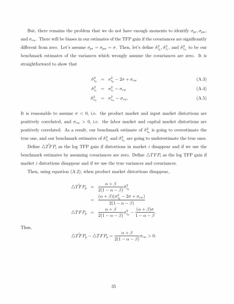
But, there remains the problem that we do not have enough moments to identify σpr, σpw,

and σrw. There will be biases in our estimates of the TFP gain if the covariances are significantly

different from zero. Let’s assume σpr = σpw = σ. Then, let’s define σ2τp

, σ2τr

, and σ2τw

to be our

benchmark estimates of the variances which wrongly assume the covariances are zero. It is

straightforward to show that

σ2τp

= σ2τp

− 2σ + σrw (A.3)

σ2τr

= σ2τr

− σrw (A.4)

σ2τw

= σ2τw

− σrw. (A.5)

It is reasonable to assume σ < 0, i.e. the product market and input market distortions are

positively correlated, and σrw > 0, i.e. the labor market and capital market distortions are

positively correlated. As a result, our benchmark estimate of σ2τp

is going to overestimate the

true one, and our benchmark estimates of σ2τr

and σ2τw

are going to underestimate the true ones.

Define ˆ△TFPi as the log TFP gain if distortions in market i disappear and if we use the

benchmark estimates by assuming covariances are zero. Define △TFPi as the log TFP gain if

market i distortions disappear and if we use the true variances and covariances.

Then, using equation (A.2), when product market distortions disappear,

ˆ△TFPp =α + β

2(1 − α − β)σ2

τp

=(α + β)(σ2

τp− 2σ + σrw)

2(1 − α − β)

△TFPp =α + β

2(1 − α − β)σ2

τp−

(α + β)σ

1 − α − β.

Thus,

ˆ△TFPp − △TFPp =α + β

2(1 − α − β)σrw > 0.

35

Similarly, when the capital market distortions disappear,

ˆ△TFPr =α(1 − β)

2(1 − α − β)σ2

τr

=α(1 − β)(σ2

τr− σrw)

2(1 − α − β)

△TFPr =α(1 − β)

2(1 − α − β)σ2

τr−

ασ − αβσrw

1 − α − β.

Then,

ˆ△TFPr − △TFPr =α

2(1 − α − β)(2σ − (1 − β)σrw) < 0.

When the labor market distortions disappear,

ˆ△TFPw =β(1 − α)

2(1 − α − β)σ2

τw

=β(1 − α)(σ2

τw− σrw)

2(1 − α − β)

△TFPw =β(1 − α)

2(1 − α − β)σ2

τw−

βσ − αβσrw

1 − α − β.

Then,

ˆ△TFPw − △TFPw =β

2(1 − α − β)(2σ − (1 − α)σrw) < 0.

As mentioned above, we do not have enough moments to identify the covariances. Instead,

we try different values of correlation (ρ) to have a sense of the magnitude of the bias in the TFP

gain estimates. We assume the correlations between the product market and input markets are

−ρ and the correlation between the labor market and capital market is ρ.

Tables A.3 and A.4 report the results. Both tables suggest that when the correlation between

the distortions is not too high (less than 0.5), eliminating the variation in the product market

distortions would yield the largest TFP gain in all three countries. In France, the TFP gain

from eliminating product market distortion variation is still larger than the gain from eliminating

other distortion variation even if the correlation is very high (ρ = 0.7).

36

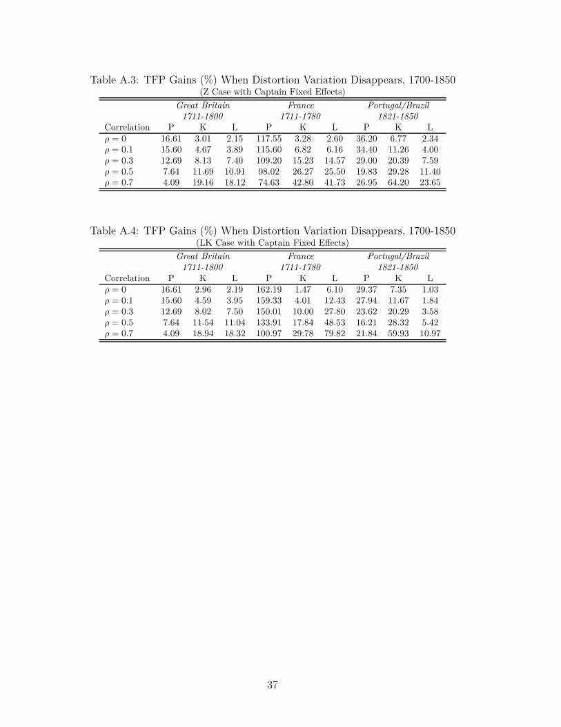
Table A.3: TFP Gains (%) When Distortion Variation Disappears, 1700-1850(Z Case with Captain Fixed Effects)

Great Britain France Portugal/Brazil1711-1800 1711-1780 1821-1850

Correlation P K L P K L P K Lρ = 0 16.61 3.01 2.15 117.55 3.28 2.60 36.20 6.77 2.34ρ = 0.1 15.60 4.67 3.89 115.60 6.82 6.16 34.40 11.26 4.00ρ = 0.3 12.69 8.13 7.40 109.20 15.23 14.57 29.00 20.39 7.59ρ = 0.5 7.64 11.69 10.91 98.02 26.27 25.50 19.83 29.28 11.40ρ = 0.7 4.09 19.16 18.12 74.63 42.80 41.73 26.95 64.20 23.65

Table A.4: TFP Gains (%) When Distortion Variation Disappears, 1700-1850(LK Case with Captain Fixed Effects)

Great Britain France Portugal/Brazil1711-1800 1711-1780 1821-1850

Correlation P K L P K L P K Lρ = 0 16.61 2.96 2.19 162.19 1.47 6.10 29.37 7.35 1.03ρ = 0.1 15.60 4.59 3.95 159.33 4.01 12.43 27.94 11.67 1.84ρ = 0.3 12.69 8.02 7.50 150.01 10.00 27.80 23.62 20.29 3.58ρ = 0.5 7.64 11.54 11.04 133.91 17.84 48.53 16.21 28.32 5.42ρ = 0.7 4.09 18.94 18.32 100.97 29.78 79.82 21.84 59.93 10.97

37

References

Allen, R. C. (2001): “The Great Divergence in European Wages and Prices from the Middle

Ages to the First World War,” Explorations in Economic History, 38(4), 411–447.

Bloom, N. (2009): “The Impact of Uncertainty Shocks,” Econometrica, 77(3), 623–685.

Chari, V., P. J. Kehoe, and E. R. McGrattan (2007): “Business Cycle Accounting,”

Econometrica, 75(3), 781–836.

Dalton, J. T., and T. C. Leung (2014): “Why is Polygyny More Prevalent in Western

Africa? An African Slave Trade Perspective,” Economic Development and Cultural Change,

62(4), 599–632.

Darity, Jr., W. (1992): “A Model of “Original Sin”: Rise of the West and Lag of the Rest,”

American Economic Review, 82(2), 162–167.

Donnan, E. (1930): Documents Illustrative of the History of the Slave Trade to America, vol. 3.

Washington, D.C.: Carnegie Institution of Washington.

Eltis, D., and S. L. Engerman (2000): “The Importance of Slavery and the Slave Trade to

Industrializing Britain,” Journal of Economic History, 60(1), 123–144.

Eltis, D., F. D. Lewis, and K. McIntyre (2010): “Accounting for the Traffic in Africans:

Transport Costs on Slaving Voyages,” Journal of Economic History, 70(4), 940–963.

Eltis, D., F. D. Lewis, and D. Richardson (2005): “Slave Prices, the African Slave Trade,

and Productivity in the Caribbean, 1674-1807,” Economic History Review, 58(4), 673–700.

Eltis, D., and D. Richardson (1995): “Productivity in the Transatlantic Slave Trade,”

Explorations in Economic History, 32, 465–484.

(2004): “Prices of African Slaves Newly Arrived in the Americas, 1673-1865: New

Evidence on Long-Run Trends and Regional Differentials,” in D. Eltis, F. D. Lewis, and K.

L. Sokoloff, editors, Slavery in the Development of the Americas, London, UK: Cambridge

University Press, 181-218.

38

(2010): Atlas of the Transatlantic Slave Trade. New Haven, CT: Yale University Press.

Fenske, J. (2012): “African Polygamy: Past and Present,” working paper.

Fenske, J., and N. Kala (2012): “Climate, Ecosystem Resilience, and the Slave Trade,”

working paper.

Gabaix, X. (2009): “Power Laws in Economics and Finance,” Annual Review of Economics,

1, 255–293.

Greif, A. (1989): “Reputation and Coalitions in Medieval Trade: Evidence on the Maghribi

Traders,” Journal of Economic History, 49(4), 857–882.

(1993): “Contract Enforceability and Economic Institutions in Early Trade: The

Maghribi Traders’ Coalition,” American Economic Review, 83(3), 525–548.

Harms, R. (2002): The Diligent: A Voyage Through the Worlds of the Slave Trade. New York,

NY: Basic Books.

Hogerzeil, S. J., and D. Richardson (2007): “Slave Purchasing Strategies and Shipboard

Mortality: Day-to-Day Evidence from the Dutch African Trade, 1751-1797,” Journal of Eco-

nomic History, 67(1), 160–190.

Hopenhayn, H. A. (1992): “Entry, Exit, and Firm Dynamics in Long Run Equilibrium,”

Econometrica, 60(5), 1127–1150.

(2011): “Firm Microstructure and Aggregate Productivity,” Journal of Money, Credit

and Banking, 43(5), 111–145.

Hsieh, C.-T., and P. J. Klenow (2009): “Misallocation and Manufacturing TFP in China

and India,” Quarterly Journal of Economics, 124(4), 1403–1448.

Hunt, E. H. (1973): Regional Wage Variations in Britain 1850-1914. Oxford, UK: Clarendon

Press.

Inikori, J. (1981): “Market Structure and the Profits of the British African Trade in the Late

Eighteenth Century,” Journal of Economic History, 41(4), 745–776.

39

Lucas, Jr., R. E. (1978): “On the Size Distribution of Business Firms,” Bell Journal of

Economics, 9(2), 508–523.

Marschak, J., and W. H. Andrews (1944): “Random Simultaneous Equations and the

Theory of Production,” Econometrica, 12(3), 143–205.

Melitz, M. J. (2003): “The Impact of Trade on Intra-Industry Reallocations and Aggregate

Industry Productivity,” Econometrica, 71(6), 1695–1725.

North, D. C. (1968): “Sources of Productivity Change in Ocean Shipping, 1600-1850,” Journal

of Political Economy, 76(5), 953–970.

Nunn, N. (2007): “Historical Legacies: A Model Linking Africa’s Past to its Current Under-

development,” Journal of Development Economics, 83(1), 157–175.

(2008): “The Long-Term Effects of Africa’s Slave Trades,” Quarterly Journal of Eco-

nomics, 128(1), 139–176.

Nunn, N., and L. Wantchekon (2011): “The Slave Trade and the Origins of Mistrust in

Africa,” American Economic Review, 101(7), 3221–3252.

Pearson, R., and D. Richardson (2001): “Business Networking in the Industrial Revolu-

tion,” Economic History Review, 54(4), 657–679.

Phelps Brown, E. H., and S. V. Hopkins (1981): A Perspective of Wages and Prices.

London, UK: Methuen.

Pollard, S. (1959): “Labour in Great Britain,” in P. Mathias and M. M. Postan, editors, The

Cambridge Economic History of Europe, vol7 : The Industrial Economies: Capital, Labour,

and Enterprise, Cambridge, UK: Cambridge University Press, 97-179.

Postma, J. M. (1990): The Dutch in the Atlantic Slave Trade 1600-1815. New York, NY:

Cambridge University Press.

Price, J. M., and P. G. E. Clemens (1987): “A Revolution of Scale in Overseas Trade:

British Firms in the Chesapeake Trade, 1675-1775,” Journal of Economic History, 47(1),

1–43.

40

Rawley, J. A. (1981): The Transatlantic Slave Trade: A History. New York, NY: W.W.

Norton and Company.

Rodney, W. (1972): How Europe Underdeveloped Africa. London: Bogle-L’Ouverture Publi-

cations.

Sicsic, P. (1992): “City-Farm Wage Gaps in Late Nineteenth-Century France,” Journal of

Economic History, 52(3), 675–695.

Song, Z. M., and G. L. Wu (2013): “Identifying Capital Market Distortions,” working paper.

Thomas, H. (1997): The Slave Trade: The Story of the Atlantic Slave Trade, 1440-1870. New

York, NY: Simon and Schuster.

Viles, P. (1972): “The Slaving Interest in the Atlantic Ports, 1763-1792,” French Historical

Studies, 7(4), 529–543.

Williamson, J. G. (1995): “The Evolution of Global Labor Markets since 1830: Background

Evidence and Hypotheses,” Explorations in Economic History, 32, 141–196.

(1996): “Globalization, Convergence, and History,” Journal of Economic History,

56(2), 277–306.

41