WP 17/22

On the Use of the Lasso for Instrumental Variables

Estimation with Some Invalid Instruments

Frank Windmeijer; Helmut Farbmacher;

Neil Davies and George Davey Smith

August 2017

http://www.york.ac.uk/economics/postgrad/herc/hedg/wps/

HEDGHEALTH, ECONOMETRICS AND DATA GROUP

On the Use of the Lasso for Instrumental VariablesEstimation with Some Invalid Instruments∗

Frank Windmeijera,d,†, Helmut Farbmacherb, Neil Daviesc,d

George Davey Smithc,d

aDepartment of Economics, University of Bristol, UKbCenter for the Economics of Aging, Max Planck Society Munich, GermanycSchool of Social and Community Medicine, University of Bristol, UK

dMRC Integrative Epidemiology Unit, Bristol, UK

August 2017

Abstract

We investigate the behaviour of the Lasso for selecting invalid instruments in lin-ear instrumental variables models for estimating causal effects of exposures onoutcomes, as proposed recently by Kang, Zhang, Cai and Small (2016, Journal ofthe American Statistical Association). Invalid instruments are such that they failthe exclusion restriction and enter the model as explanatory variables. We showthat for this setup, the Lasso may not consistently select the invalid instruments ifthese are relatively strong. We propose a median estimator that is consistent whenless than 50% of the instruments are invalid, but its consistency does not dependon the relative strength of the instruments, or their correlation structure. We showthat this estimator can be used for adaptive Lasso estimation, with the result-ing estimator having oracle properties. The methods are applied to a Mendelianrandomisation study to estimate the causal effect of BMI on diastolic blood pres-sure, using data on individuals from the UK Biobank, with 96 single nucleotidepolymorphisms as potential instruments for BMI.

Key Words: causal inference, instrumental variables estimation, invalid instru-ments, Lasso, Mendelian randomisation

∗This research was partly funded by the Medical Research Council (MC_UU_12013/9). Helpfulcomments were provided by Kirill Evdokimov, Chirok Han, Whitney Newey, Hyunseung Kang, ChrisSkeels, Martin Spindler, Jonathan Temple, Ian White and seminar participants at Amsterdam, Bristol,Lausanne, Monash, Oxford, Princeton, Seoul, Sydney, the RES Conference Brighton, the Info-MetricsConference Cambridge and the UK Causal Inference Meeting London.

†f.windmeijer@bristol.ac.uk

1

1 Introduction

Instrumental variables estimation is a procedure for the identification and estimation

of causal effects of exposures on outcomes where the observed relationships are con-

founded by non-random selection of exposure. This problem is likely to occur in ob-

servational studies, but also in randomised clinical trials if there is selective participant

non-compliance. An instrumental variable (IV) can be used to solve the problem of

non-ignorable selection. In order to do this, an IV needs to be associated with the ex-

posure, but only associated with the outcome indirectly through its association with the

exposure. The former condition is referred to as the ‘relevance’ and the latter as the

‘exclusion’ condition. Examples of instrumental variables are quarter-of-birth for educa-

tional achievement to determine its effect on wages, see Angrist and Krueger (1991), ran-

domisation of patients to treatment as an instrument for actual treatment when there is

non-compliance, see e.g. Greenland (2000), and Mendelian randomisation studies use IVs

based on genetic information, see e.g. Lawlor et al. (2008). For recent reviews and further

examples see e.g. Clarke and Windmeijer (2012), Imbens (2014), Burgess et al. (2015)

and Kang et al. (2016).

Whether instruments are relevant can be tested from the observed association between

exposure and instruments. The effects on the standard linear IV estimator of ‘weak in-

struments’, i.e. the case where instruments are only weakly associated with the exposure

of interest, have been derived for the linear model using weak instrument asymptotics by

Staiger and Stock (1997). This has led to the derivation of critical values for the simple F-

test statistic for testing the null of weak instruments by Stock and Yogo (2005). Another

strand of the literature focuses on instrument selection in potentially high-dimensional

settings, see e.g. Belloni et al. (2012), Belloni et al. (2014), Chernozhukov et al. (2015)

and Lin et al. (2015), where the focus is on identifying important covariate effects and

selecting optimal instruments from a (large) set of a priori valid instruments, where

optimality is with respect to the variance of the IV estimator.

In this paper we consider violations of the exclusion condition of the instruments,

following closely the setup of Kang et al. (2016) for the linear IV model where some of

the available instruments can be invalid in the sense that they can have a direct effect on

the outcomes or are associated with unobserved confounders. Kang et al. (2016) propose

2

a Lasso type procedure to identify and select the set of invalid instruments. Liao (2013)

and Cheng and Liao (2015) also considered shrinkage estimation for identification of

invalid instruments, but in their setup there is a subset of instruments that is known

to be valid and that contains sufficient information for identification and estimation of

the causal effects. In contrast, Kang et al. (2016) do not assume any prior knowledge

about which instruments are potentially valid or invalid. This is a similar setup as in

Andrews (1999) who proposed a selection procedure using information criteria based on

the so-called J-test of over-identifying restrictions, as developed by Sargan (1958) and

Hansen (1982). The Andrews (1999) setup is more general than that of Kang et al. (2016)

and requires a large number of model evaluations, which has a negative impact on the

performance of the selection procedure.

This paper assesses the performance of the Kang et al. (2016) Lasso type selection

and estimation procedure in their setting of a fixed number of potential instruments. If

the set of invalid instruments were known, the oracle Two-Stage Least Squares (2SLS)

estimator would be the estimator of choice in their setting. As the focus is estimation of

and inference on the causal effect parameter, denoted by β, and as the standard Lasso

approach does not have oracle properties, see e.g. Zou (2006), we show how the adaptive

Lasso procedure of Zou (2006) can be used in order to obtain an estimator with oracle

properties. In order to do so, we propose an initial consistent estimator of the parameters

that is consistent also when the irrepresentable condition for consistent Lasso selection

of Zhao and Yu (2006) and Zou (2006) fails.

Applying the irrepresentable condition to this IV setup, we derive conditions under

which the Lasso method does not consistently select the invalid instruments. As is

well known from Zhao and Yu (2006), Zou (2006), Meinshausen and Bühlmann (2006)

and Wainwright (2009), certain correlation structures of the variables prevent consistent

selection. New in our results are the conditions on the strength of the invalid instruments

relative to that of the valid ones that result in violations of the irrepresentable condition,

where the strength of an instrument is its standardised effect on the exposure. From this

we can show that consistent selection of the invalid instruments may not be possible if

these are relatively strong, even when less than 50% of the instruments are invalid, which

is a sufficient condition for the identification of the parameters.

We show that under the condition that less than 50% of the instruments are invalid, a

3

simple median type estimator is a consistent estimator for the parameters in the model,

independent of the strength of the invalid instruments relative to that of the valid in-

struments, or their correlation structure. It can therefore be considered for use in the

adaptive Lasso procedure as proposed by Zou (2006). With n the sample size, we show

that the median estimator converges at the√n rate, but with an asymptotic bias, as the

limiting distribution is that of an order statistic. It does, however, satisfy the conditions

for the adaptive Lasso procedure to enjoy oracle properties.

Because of this oracle property, and as in practice instrument strength is very likely

to vary by instruments and invalid instruments could be relatively strong, it will be

important to consider our adaptive Lasso approach for assessing instrument validity and

estimating causal effects. In Mendelian randomisation studies it is clear that genetic

markers have differential impacts on exposures from examining the results from genome

wide association studies and one cannot rule out ex-ante that invalid instruments with a

direct effect are also stronger predictors for the exposure.1

The next section, Section 2, introduces the model and the Lasso estimator as proposed

by Kang et al. (2016). In Section 3, we derive the irrepresentable condition for this

particular Lasso selection problem and present the result on the relationship between

the relative strengths of the instruments and consistent selection. Section 4 presents the

median estimator, establishes its consistency and shows that its asymptotic properties

are such that the adaptive Lasso estimator enjoys oracle properties. Section 5 presents

some Monte Carlo simulation results. In Section 6, we link the Andrews (1999) method

to the Lasso selection problem and show how the test of overidentifying restrictions can

be used as a stopping rule. Section 7 investigates how close the behaviour of the adaptive

Lasso estimator is to that of the oracle 2SLS estimator in the Monte Carlo simulations,

by comparing the performances of the Wald tests on the causal parameter under the null

for different sample sizes. It further discusses more generally the issue of information

content for this estimation problem, including that of weak instruments. In Section 8,

the methods are applied to a Mendelian randomisation study to estimate the causal effect

of Body Mass Index (BMI) on diastolic blood pressure using data on individuals from

1Bowden et al. (2015) and Kolesar et al. (2015) allow for all instruments to be invalid and show thatthe causal effect can be consistently estimated if the number of instruments increases with the samplesize under the assumption of uncorrelatedness of the instrument strength and their direct effects on theoutcome variable.

4

the UK Biobank, with 96 single nucleotide polymorphisms as potential instruments for

BMI. Section 9 concludes.

The following notation is used in the remainder of the paper. For a full column rank

matrix X with n rows,MX = In−PX , where PX = X (X′X)−�X′ is the projection onto

the column space of X, and In is the n-dimensional identity matrix. A k-vector of ones

is denoted ιk. The lp-norm is denoted by ‖.‖p, and the l�-norm, ‖.‖�, denotes the numberof non-zero components of a vector. We use ‖.‖∞ to denote the maximal element of a

vector.

2 Model and Lasso Estimator

We follow Kang, Zhang, Cai and Small (2016) (KZCS from now on), who considered the

following potential outcomes model. For i = 1, ..., n, let Y �d,��i , be the potential outcome if

the individual i were to have exposure d and instrument values z. The observed outcome

for an individual i is denoted by the scalar Yi, the treatment by the scalar Di and the

vector of L potential instruments by Zi.. The instruments may not all be valid and

can have a direct or indirect effect. For two possible values of the exposure d∗, d and

instruments z∗, z, assume the following potential outcomes model

Y�d∗,�∗�i − Y �d,��i = (z∗ − z)′φ+ (d∗ − d) β (1)

E[Y��,��i |Zi.

]= Z′i.ψ, (2)

where φmeasures the direct effect of z on Y , andψ represents the presence of unmeasured

confounders that affect both the instruments and the outcome.

We have a random sample {Yi, Di,Z′i.}ni��. Combining (1) and (2), the observed data

model for the random sample is given by

Yi = Diβ + Z′i.α+ εi, (3)

where α = φ+ψ;

εi = Y��,��i − E

[Y��,��i |Zi.

]

and hence E [εi|Zi.] = 0. For ease of exposition, we further assume that E [ε�i |Zi.] = σ�.The KZCS definition of a valid instrument is then linked to the exclusion restriction

and given as follows: Instrument j, j ∈ {1, ..., L}, is valid if αj = 0 and it is invalid if

5

αj �= 0. As in the KZCS setting, we are interested in the identification and estimationof the scalar treatment effect β in large samples with a fixed number L of potential

instruments.

Let y and d be the n-vectors of n observations on {Yi} and {Di} respectively, and letZ be the n× L matrix of potential instruments. As an intercept is implicitly present inthe model, y, d and the columns of Z have all been taken in deviation from their sample

means. Following the notation of Zou (2006), let ZA be the set of invalid instruments,

A = {j : αj �= 0} and αA the associated coefficient vector. The oracle Instrumental

Variables, or Two-Stage Least Squares (2SLS) estimator is obtained when the set ZA is

known. Let RA =[d ZA

], the oracle 2SLS estimator is then given by

θor =

(βorαA

)= (R′

APZRA)−�R′APZy. (4)

Let d = PZd, with individual elements Di, then θor is the OLS estimator in the model

Yi = Diβ + Z′A,i.αA + ξi,

where ξi is defined implicitly, and hence

αA =(Z′AMdZA

)−�Z′AMdy

=(Z′AMdZA

)−�Z′AMdPZy. (5)

The oracle 2SLS estimator for β is given by

βor =(d′MZ�d

)−�d′MZ�y.

Under standard assumptions, as defined below,

√n(βor − β

)d−→ N

(0, σ�β��

), (6)

where

σ�β�� = σ�(E [Zi.Di]

′E [Zi.Z′i.]−�E [Zi.Di]− E [ZA,i.Di]

′E[ZA,i.Z

′A,i.

]−�E [ZA,i.Di]

)−�.

(7)

The vector d is the linear projection of d on Z. If we define γ = (Z′Z)−� Z′d, then

d = Zγ, or Di = Z′i.γ. We specify

Di = Z′i.γ + vi, (8)

6

where γ = E [Zi.Z′i.]−�E [Zi.Di], and hence E [Zi.vi] = 0. Further, as in KZCS, let

Γ = E [Zi.Z′i.]−�E [Zi.Yi] = γβ +α. Then define πj as

πj ≡Γjγj= β +

αjγj, (9)

for j = 1, ..., L. Theorem 1 in KZCS states the conditions under which, given knowledge

of γ and Γ, a unique solution exists for values of β and αj. A necessary and sufficient

condition to identify β and the αj is that the valid instruments form the largest group,

where instruments form a group if they have the same value of π. Corollary 1 in KZCS

then states a sufficient condition for identification. Let s = ||α||� be the number ofinvalid instruments. A sufficient condition is that s < L/2, as then clearly the largest

group is formed by the valid instruments.

In model (3), some elements of α are assumed to be zero, but it is not known ex-ante

which ones they are and the selection problem therefore consists of correctly identifying

those instruments with non-zero α. KZCS propose to estimate the parameters α and β

by using l� penalisation on α and to minimise(α�n�, β

�n�)= argmin

α,β

1

2‖PZ (y − dβ − Zα) ‖�� + λn‖α‖�, (10)

where ‖α‖� =∑

j |αj| and the squared l� norm is (y − dβ − Zα)′PZ (y − dβ − Zα).This method is closely related to the Lasso, and the regularization parameter λn deter-

mines the sparsity of the vector α�n�. From (5), a fast two-step algorithm is proposed as

follows. For a given λn solve

α�n� = argminα

1

2‖MdPZy −MdZα‖

�� + λn‖α‖� (11)

and obtain β�n�by

β�n�=d′(y − Zα�n�

)

d′d. (12)

In order to find α�n� in (11), the Lasso modification of the LARS algorithm of Efron,

Hastie, Johnstone and Tibshirani (2004) can be used and KZCS have developed an R-

routine for this purpose, called sisVIVE (some invalid and some valid IV estimator),

where the regularisation parameter λn is obtained by cross-validation.

The standard Lasso estimator does not have oracle properties, see e.g. Zou (2006).

In order to obtain an adaptive Lasso estimator with oracle properties, we propose an

7

initial consistent estimator that is well behaved also when the irrepresentable condition

for consistent Lasso variable selection fails. In the next section we show under what con-

ditions the Lasso selection of invalid instruments is inconsistent using the irrepresentable

condition of Zhao and Yu (2006) and Zou (2006). We show that this does depend on

the strength of the invalid instruments relative to that of the valid ones in combination

with the number of invalid instruments, and the correlation structure of the instruments.

KZCS did show analytically that the performance of the Lasso estimator is influenced

by these factors, but did not relate them to consistent selection. In particular, we show

how relatively strong invalid instruments may result in the Lasso method selecting the

valid instruments as invalid in large samples.

Under the assumptions specified below, γ and Γ can be consistently estimated by

γ and Γ = (Z′Z)−� Z′y respectively. Let πj = Γj/γj, for j = 1, ..., L. We show that

the median of the πj is a consistent estimator for β when s < L/2, without any further

restrictions on the relative strengths or correlations of the instruments, and that the

asymptotic properties of this estimator are such that the resulting estimator for α can

be used for the adaptive Lasso of Zou (2006). We therefore obtain a desired estimator

with the same limiting distribution as the oracle 2SLS estimator (6), also when the

irrepresentable condition is violated, as long as s < L/2, which is the same condition as

the sufficient condition of KZCS for identification.

For the random variables and i.i.d. sample {Yi, Di,Z′i.}ni��, and model (3) and (8), we

assume throughout that the following conditions hold:

Assumption 1 E [Zi.Z′i.] = Q is full rank.

Assumption 2 plim (n−�Z′Z) = E [Zi.Z′i.]; plim (n−�Z′d) = E [Zi.Di]; plim (n−�Z′ε) =

E [Zi.εi] = 0.

Assumption 3 γ = (E [Zi.Z′i.])−�E [Zi.Di], γj �= 0, j = 1, ..., L.

The setting is thus a relatively straightforward one with fixed parameters β, α and

γ, and fixed number L � n of potential instruments. This is the setting under which

the oracle 2SLS estimator has the limiting distribution (6), and is a setting of interest

in many applications. To identify in this simple setting an ex-ante unknown subset of

8

invalid instruments using the Lasso is challenging, as highlighted in the next section.

In the Monte Carlo simulation section we present results confirming that the adaptive

Lasso estimator we propose performs well in large samples, but may not perform well

in small samples. A small sample is essentially a small information setting, which we

discuss further in Section 7.

For the case of many weak instruments, even the oracle 2SLS estimator would not

be the estimator of choice, due to its poor asymptotic performance, and the median

estimator may not be consistent. Oracle estimators with better asymptotic properties

in this setting are the Limited Information Maximum Likelihood (LIML) estimator, see

Bekker (1994) and Hansen, Hausman and Newey (2008), or the Continuous Updating

Estimator (CUE), see Newey and Windmeijer (2009). Selection of invalid instruments in

this setting is outside the scope of this paper.

3 Irrepresentable Condition

As Z′MdMdPZy = Z′MdPZy = Z

′Mdy, it follows that

‖Md (PZy − Zα) ‖�� = y′PZMdPZy − 2y

′MdZα+α′Z′MdZα

= y′PZMdPZy − 2y′Zα+α′Z′Zα,

where Z =MdZ. As

‖y − Zα‖�� = y′y − 2y′Zα+α′Z′Zα,

it follows that the Lasso estimator α�n� as defined in (11) can equivalently be obtained

as

α�n� = argminα

1

2‖y − Zα‖�� + λn‖α‖�. (13)

This minimization problem looks very much like a standard Lasso approach with Z as

explanatory variables. However, an important difference is that Z does not have full rank,

but its rank is equal to L− 1. This is related to the standard Lasso case where we havean overcomplete dictionary implying that the OLS solution is not feasible. Intuitively,

we cannot set λn = 0 in (13) as we have to shrink at least one element of α to zero

to identify the parameter β. All just-identified models with L− 1 instruments includedas invalid result in a residual correlation of 0, and hence λn = 0 does not lead to a

9

unique 2SLS estimator. Therefore, when using the LARS/Lasso algorithm, it has to

start from a model without any instruments included in the model as invalid, and at the

last LARS/Lasso step one instrument is excluded from the model, i.e. treated as valid.

When L − 1 instruments have been selected as invalid and included in the model, theresulting Lasso estimator is the (just identified) 2SLS estimator and this final model is

the model for which λn = 0. Clearly, it can then be the case that the LARS/Lasso path

is such that it does not include a model where all invalid instruments have been selected

as such, which is the case when the final instrument selected as valid is in fact invalid.

We follow Zhao and Yu (2006) and Zou (2006) who developed the irrepresentable

conditions for consistent Lasso variable selection. Let C = plim(n−�Z′Z

). As before,

let A = {j : αj �= 0} and assume wlog that A = {1, 2, ..., s}.2 Let

C =

[C�� C′

��

C�� C��

], (14)

where C�� is an s × s matrix. Further, define An ={j : α

�n�j �= 0

}. Let s (α�) denote

the vector sgn (α�), where α� = αA = (α�, ..., αs)′, sgn (a) = 1 if a > 0 and sgn (a) = −1

if a < 0. A sufficient condition for consistent Lasso variable selection, meaning that

limn→∞ P(An = A

)= 1, is the irrepresentable condition

∥∥C��C−��� s (α�)

∥∥∞ < 1. (15)

If∥∥C��C

−��� s (α�)

∥∥∞ > 1, then the lasso variable selection is inconsistent, see Zhao and

Yu (2006) and Zou (2006).

Partition Q = plim (n−�Z′Z) and γ commensurate with the partitioning of C as

Q =

[Q�� Q′

��

Q�� Q��

], γ =

(γ�γ�

), (16)

where the instruments have been standardised such the diagonal elements of Q are equal

to 1. Then for the Lasso specification (13) we have the following result.

Proposition 1 Consider the observational models (3) and (8) under Assumptions 1, 2,

and 3. Let C = plim(n−�Z′Z

); Q = plim (n−�Z′Z); and C��, C��, Q��, Q��, Q��, γ�

2We will use subscripts A and � interchangeably from here onwards, and subscript � for associationswith the set A� � {j � α� � �}.

10

and γ� as specified in (14) and (16). Then C��C−��� is given by

C��C−��� = Q��Q

−��� − Q��γ�

γ ′� + γ′�Q��Q

−���

γ ′�Q��γ�, (17)

where

Q�� = Q�� −Q��Q−���Q

′�� = plim

(n−�Z′�MZ�Z�

).

Proof. See Appendix A.1.

Proposition 1 shows that consistent selection of the instruments is not only affected

by the correlation structure of the instruments, but also by the values of γ� and γ�. The

next Proposition derives conditions on γ� and γ� under which consistent selection is not

possible.

Proposition 2 Under the assumptions of Proposition 1, the Lasso variable selection is

not consistent if

|γ ′�s (α�)| > ‖γ�‖� .

Proof. It follows from (17) that

∣∣γ ′�C��C−��� s (α�)

∣∣ = |γ ′�s (α�)| .

Therefore,

‖γ�‖�∥∥C��C−��� s (α�)

∥∥∞ ≥ |γ ′�s (α�)|

∥∥C��C−��� s (α�)∥∥∞ ≥ |γ ′�s (α�)|

‖γ�‖�.

Hence,∥∥C��C

−��� s (α�)

∥∥∞ > 1 if |γ

′�s (α�)| > ‖γ�‖�.

Remark 1 If s (α�) = s (γ�), then |γ ′�s (α�)| = ‖γ�‖�, its maximum. Regardless ofthe correlation structure of the instruments, the Lasso variable selection is therefore not

consistent in that case if ‖γ�‖� > ‖γ�‖�, i.e. when the invalid instruments are stronger(in l�-norm) than the valid ones.

From Proposition 1 we can investigate consistent selection for various cases of interest.

Related to the Monte Carlo simulations in KZCS and below in Section 5, Corollary 1

considers the case with γ� = γ�ιs and γ� = γ�ιL−s.

11

Corollary 1 If γ� = γ�ιs and γ� = γ�ιL−s, then |γ ′�s (α�)| > ‖γ�‖� if∣∣∣ γ�γ�∣∣∣ |ι′ss (α�)| >

L − s. Let g = |ι′ss (α�)|, then it follows that selection is inconsistent if∣∣∣ γ�γ�∣∣∣ g > L − s.

Hence if g = s,∣∣∣∣C��C−��� s (α�)

∣∣∣∣∞ > 1 if s > L/

(1 +

∣∣∣ γ�γ�∣∣∣).

When instruments are uncorrelated, such thatQ = IL� it follows that∥∥C��C

−��� s (α�)

∥∥∞ <

1 if s < L−∣∣∣ γ�γ�∣∣∣ g. Hence if g = s, limn→∞ P

(An = A

)= 1 if s < L/

(1 +

∣∣∣ γ�γ�∣∣∣).

Remark 2 For equal strength instruments, γ� = γ�, the result of Corollary 1 shows

that the Lasso approach will not select the invalid instruments consistently for all possible

configurations of α� if s > L/2. For uncorrelated equal strength instruments, the selection

is consistent for all possible configurations of α� if s < L/2.

Remark 3 The result of Corollary 1 shows that for the uncorrelated instruments design,

the condition s < L/2, whilst sufficient for the formal identification result of Theorem 1

in KZCS, is not a sufficient condition for consistent selection of the invalid instruments,

as the number of invalid instruments permitted for consistent selection shrinks with an

increasing relative strength of the invalid instruments, |γ�/γ�|.

Remark 4 It follows from Corollary 4 in Zhao and Yu (2006), that if the columns of Z

are standardised such that the diagonal elements of C are equal to 1, with the correlations

bounded from 1, then the irrepresentable condition holds and the selection is consistent

when s = 1, irrespective of the values of γ.

4 A Consistent Estimator when s < L/� and Adap-tive Lasso

As the results above highlight, the LARS/Lasso path may not include the correct model,

leading to an inconsistent estimator of β. This is the case even if less than 50% of the

instruments are invalid because of differential instrument strength and/or correlation

patterns of the instruments. In this section we present an estimation method that con-

sistently selects the invalid instruments when less than 50% of the potential instruments

are invalid. This is the same condition as that for the LARS/Lasso selection to be guar-

anteed to be consistent for equal strength uncorrelated instruments, but the proposed

12

estimator below is consistent when the instruments have differential strength and/or have

a general correlation structure.

We consider the adaptive Lasso approach of Zou (2006) using an initial consistent

estimator of the parameters. In the standard linear case, the OLS estimator in the model

with all explanatory variables included is consistent. As explained in Section 3, in the

instrumental variables model this option is not available. We build on the result of Han

(2008), who shows that the median of the L IV estimates of β using one instrument at

the time is a consistent estimator of β in a model with invalid instruments, but where

the instruments cannot have direct effects on the outcome, unless the instruments are

uncorrelated.

As before, let Γ = (Z′Z)−� Z′y; γ = (Z′Z)−� Z′d, and let π be the L-vector with j-th

element

πj =Γjγj. (18)

Under the standard assumptions, Theorem 1 below shows that the median of the πj,

denoted βm, is a consistent estimator for β when s < L/2, without any further restrictions

on the relative strengths or correlations of the instruments. Theorem 1 also shows that√n(βm − β

)converges in distribution to that of an order statistic. From these results it

follows that the consistent estimator αm = Γ− γβm can be used for the adaptive Lassoapproach of Zou (2006), resulting in oracle properties of the resulting estimator of β.

Theorem 1 Under model specifications (3) and (8) with Assumptions 1 - 3, let π be the

L-vector with elements as defined in (18). If s < L/2, then the estimator βm defined as

βm = median (π)

is a consistent estimator for β,

plim(βm

)= β.

Let π� be the L− s vector with elements πj, j = s+1, ..., L. The limiting distribution ofβm is given by √

n(βm − β

)d−→ q�l�,L−s,

where for L odd, q�l�,L−s is the l-th order-statistic of the limiting normal distribution of√n (π� − βιL−s), where l is determined by L, s and the signs of δj = α�

γ�, j = 1, ..., s.

13

For L even, q�l�,L−s is defined as the average of either the [l] and [l − 1] order statistics,or the [l] and [l + 1] order statistics.

Proof. Under the stated assumptions,

plim(Γ)= γβ +α;

plim (γ) = γ.

Hence

plim (πj) =γjβ + αj

γj= β +

αjγj,

for j = 1, ..., L. As s < L/2, more than 50% of the αs are equal to zero and hence it

follows that more than 50% of the elements of plim (π) are equal to β. Using a continuity

theorem, it then follows that

plim(βm

)= median {plim (π)} = β.

For the limiting distribution, let δ� be the s-vector with elements

δj =αjγj,

for j = 1, ..., s. Let δ =(δ′� 0′L−s

)′. Partition π accordingly as π =

(π′� π′�

)′.

Under the standard conditions, the limiting distribution of π is given by

√n (π − (βιL + δ))

d−→ N (0,Σπ) .

As βm = median (π),

√n(βm − β

)=

√n (median (π)− β)

= median(√n (π − βιL)

).

As√n (π − βιL) =

( √n (π� − (βιs + δ�)) +

√nδ�√

n (π� − βιL−s)

),

it follows that

√n(βm − β

)= median

(√n (π − βιL)

) d−→ q�l�,L−s.

14

Given the consistent estimator βm, we obtain a consistent estimator for α as

αm = (Z′Z)

−�Z′(y − dβm

)= Γ− γβm,

which can then be used for the adaptive Lasso specification of (13) as proposed by Zou

(2006). The adaptive Lasso estimator for α is defined as

α�n�ad = argminα

1

2‖y − Zα‖�� + λn

L∑

l��

|αl||αm,l|υ

, (19)

and, for given values of υ can be estimated straightforwardly using the LARS algorithm,

see Zou (2006). The resulting adaptive Lasso estimator for β is obtained as

β�n�

ad =d′(y − Zα�n�ad

)

d′d.

As the result for the limiting distribution of the median estimator shows, βm, although

converging at the√n rate, has an asymptotic bias. This clearly also results in an as-

ymptotic bias of αm. As√n (αm −α) = Op (1), Theorem 2 together with Remark 1 in

Zou (2006) states the following properties of the adaptive Lasso estimator α�n�ad , where

Aad,n ={j : α

�n�ad,j �= 0

}.

Proposition 3 Suppose that λn = o (√n) and (

√n)ν−�

λn →∞, then the adaptive Lassoestimator α�n�ad satisfies

1. Consistency in variable selection: limn→∞ P(Aad,n = A

)= 1.

2. Asymptotic normality:√n(α�n�ad,A −αA

)d−→ N

(0, σ�C−���

).

Proof. See Zou (2006), Theorem 2 and Remark 1.

From the results of Proposition 3, it follows that the limiting distribution of β�n�

ad is

that of the oracle 2SLS estimator, as stated in the next Corollary.

Corollary 2 Under the conditions of Proposition 3, the limiting distribution of the adap-

tive Lasso estimator β�n�

ad is given by

√n(β�n�

ad − β)

d−→ N(0, σ�β��

), (20)

with σ�β�� as defined in (7).

15

5 Some Simulation Results

5.1 Equal strength instruments

We start with presenting some estimation results from a Monte Carlo exercise which is

similar to that in KZCS. The data are generated from

Yi = Diβ + Z′i.α+ εi

Di = Z′i.γ + vi,

where (εivi

)∼ N

((00

),

(1 ρρ 1

));

Zi. ∼ N (0, IL) ;

and we set β = 0; L = 10; ρ = 0.25; s = 3, and the first s elements of α are equal

to a = 0.2. Further, γ� = γ�ιs and γ� = γ�ιL−s with γ� = γ� = 0.2. Note that none

of the estimation results presented here and below depend on the value of β. Table 1

presents estimation results for estimators of β in terms of bias, standard deviation, root

mean squared error (rmse) and median absolute deviation (mad) for 1000 replications

for sample sizes of n = 500, n = 2000 and n = 10, 000.

The information content for IV estimation can be summarised by the concentration

parameter, see Rothenberg (1984). For the oracle estimation of β by 2SLS, the concen-

tration parameter is given by µ�n = γ′�Z

′�MZ�Z�γ�/σ

�v. For this data generating process

with independent instruments, the concentration parameter is therefore approximately

n (L− s) (0.2�) and hence equal to 140 , 560 and 2800 for the three sample sizes. Thecorresponding population F-statistics are equal to n (0.2�), or 20, 80 and 400 for the

sample sizes 500, 2000 and 10, 000 respectively. The F-statistic is a test for H� : γ� = 0.

We will discuss information content for the Lasso selection in more detail in Section

7, but the (squared) Signal to Noise Ratio (SNR), denoted by η�, is defined as

η� =α′�C��α�σ�ε

,

and is here equal to 0.084.

The "2SLS" results are for the naive 2SLS estimator of β that treats all instruments

as valid. The probability limit of this estimator is given by

plim(βnaive

)= β +

γ ′Qα

γ ′Qγ= β +

γ ′�Q��α� + γ′�Q��α�

γ ′�Q��γ� + 2γ′�Q��γ� + γ

′�Q��γ�

. (21)

16

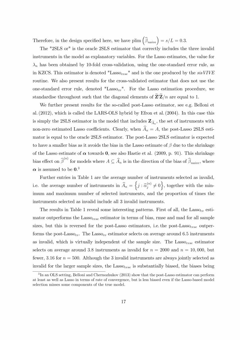
Therefore, in the design specified here, we have plim(βnaive

)= s/L = 0.3.

The "2SLS or" is the oracle 2SLS estimator that correctly includes the three invalid

instruments in the model as explanatory variables. For the Lasso estimates, the value for

λn has been obtained by 10-fold cross-validation, using the one-standard error rule, as

in KZCS. This estimator is denoted "Lassocvse" and is the one produced by the sisVIVE

routine. We also present results for the cross-validated estimator that does not use the

one-standard error rule, denoted "Lassocv". For the Lasso estimation procedure, we

standardise throughout such that the diagonal elements of Z′Z/n are equal to 1.

We further present results for the so-called post-Lasso estimator, see e.g. Belloni et

al. (2012), which is called the LARS-OLS hybrid by Efron et al. (2004). In this case this

is simply the 2SLS estimator in the model that includes ZA�, the set of instruments with

non-zero estimated Lasso coefficients. Clearly, when An = A, the post-Lasso 2SLS esti-

mator is equal to the oracle 2SLS estimator. The post-Lasso 2SLS estimator is expected

to have a smaller bias as it avoids the bias in the Lasso estimate of β due to the shrinkage

of the Lasso estimate of α towards 0, see also Hastie et al. (2009, p. 91). This shrinkage

bias effect on β�n�for models where A ⊆ An is in the direction of the bias of βnaive, where

α is assumed to be 0.3

Further entries in Table 1 are the average number of instruments selected as invalid,

i.e. the average number of instruments in An ={j : α

�n�j �= 0

}, together with the min-

imum and maximum number of selected instruments, and the proportion of times the

instruments selected as invalid include all 3 invalid instruments.

The results in Table 1 reveal some interesting patterns. First of all, the Lassocv esti-

mator outperforms the Lassocvse estimator in terms of bias, rmse and mad for all sample

sizes, but this is reversed for the post-Lasso estimators, i.e. the post-Lassocvse outper-

forms the post-Lassocv. The Lassocv estimator selects on average around 6.5 instruments

as invalid, which is virtually independent of the sample size. The Lassocvse estimator

selects on average around 3.8 instruments as invalid for n = 2000 and n = 10, 000, but

fewer, 3.16 for n = 500. Although the 3 invalid instruments are always jointly selected as

invalid for the larger sample sizes, the Lassocvse is substantially biased, the biases being

3In an OLS setting, Belloni and Chernozhukov (2013) show that the post-Lasso estimator can performat least as well as Lasso in terms of rate of convergence, but is less biased even if the Lasso-based modelselection misses some components of the true model.

17

larger than twice the standard deviations. The post-Lassocvse estimator performs best,

but is still outperformed by the oracle 2SLS estimator at n = 10, 000. Although the

post-Lassocvse estimator has a larger standard deviation than the Lassocvse estimator, it

has a smaller bias, rmse and mad for all sample sizes.

Table 1. Estimation results for 2SLS and Lasso estimators for β; L = 10, s = 3, γ� = γ�av. # instr freq. all

selected as invalid invalid instrβ bias std dev rmse mad [min, max] selectedn = 5002SLS 0.2966 0.0808 0.3074 0.2944 0 02SLS or 0.0063 0.0843 0.0845 0.0570 3 1Lassocv 0.1384 0.0965 0.1687 0.1352 6.41 [2,9] 0.990Post-Lassocv 0.1169 0.1136 0.1630 0.1143Lassocvse 0.2206 0.0847 0.2363 0.2174 3.16 [0,8] 0.664Post-Lassocvse 0.0905 0.1243 0.1537 0.0994n = 20002SLS 0.3019 0.0387 0.3044 0.3007 0 02SLS or 0.0047 0.0422 0.0424 0.0285 3 1Lassocv 0.0721 0.0509 0.0882 0.0705 6.64 [3,9] 1Post-Lassocv 0.0617 0.0577 0.0845 0.0644Lassocvse 0.1140 0.0430 0.1218 0.1165 3.76 [3,8] 1Post-Lassocvse 0.0277 0.0521 0.0590 0.0387n = 10, 0002SLS 0.2996 0.0177 0.3002 0.2992 0 02SLS or 0.0006 0.0182 0.0182 0.0126 3 1Lassocv 0.0317 0.0236 0.0395 0.0311 6.44 [3,9] 1Post-Lassocv 0.0272 0.0267 0.0380 0.0282Lassocvse 0.0479 0.0187 0.0514 0.0489 3.81 [3,9] 1Post-Lassocvse 0.0118 0.0238 0.0265 0.0176Notes: Results from 1000 MC replications; β = 0; ρ = 0.25; a = 0.2; γ�= 0.2

Figures 1a and 1b illustrate the different behaviours of the Lasso and post-Lasso

estimators. Figure 1a shows the bias and standard deviations of the two estimators for

different values of λ/n, for the design above with n = 2000, again from 1000 replications.

It is clear that the Lasso estimator exhibits a positive bias for all values of λ, declining

from that of the naive 2SLS estimator to the minimum bias of 0.0664 at λ/n = 0.0060.

In contrast, the post-Lasso estimator is (much) less biased, obtaining its minimum bias

18

of 0.0068 at the value of λ/n of 0.0965. Figure 1b displays the same information but now

as a function of the LARS steps, where additional variables enter the model (we have

omitted 3 replications where there were Lasso steps). At step 3, the correct 3 invalid

instruments have been selected 991 times out of the 997 replications, and the post-Lasso

estimator has a bias there of 0.0058, only fractionally larger than that of the oracle 2SLS

estimator. In contrast, the Lasso estimator for β still has a substantial upward bias at

step 3. Its bias decreases from 0.116 at step 3 to a minimum of 0.0650 at step 8. The bias

of the post-Lasso estimator increases again after step 3, reaching the same bias as the

Lasso estimator at the last step, as there λn = 0 and the Lasso and post-Lasso estimators

are equal.

Figures 1a and 1b. Bias and standard deviations of Lasso and post-Lasso estimators as

functions of λ/n, and LARS steps. Same design as in Table 1, n = 2000. 3 replications out of

1000 omitted in 1b due to Lasso steps.

As the results in Table 1 show, the difference in bias between the Lasso and post-Lasso

estimators is larger for the cvse procedure compared to the cv procedure, as the cvse

procedure selects a larger value for λn and hence shrinks the α coefficients more towards

0. This results in a larger bias in the estimator for β, as depicted in Figure 1a.

Table 2 presents results for the median and Adaptive Lasso estimators. The estima-

tion results for the adaptive Lasso are based on setting υ = 1. The resulting estimators

are denoted "ALasso". As L is even here, the median is defined as βm =(π�� + π��

)/2,

19

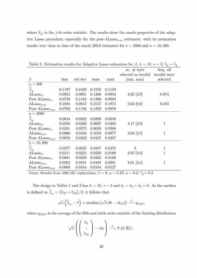
where π�j� is the j-th order statistic. The results show the oracle properties of the adap-

tive Lasso procedure, especially for the post-ALassocvse estimator, with its estimation

results very close to that of the oracle 2SLS estimator for n = 2000 and n = 10, 000.

Table 2. Estimation results for Adaptive Lasso estimators for β; L = 10, s = 3, γ� = γ�av. # instr freq. all

selected as invalid invalid instrβ bias std dev rmse mad [min, max] selectedn = 500

βm 0.1197 0.1029 0.1578 0.1159ALassocv 0.0952 0.0981 0.1366 0.0934 4.62 [2,9] 0.974Post-ALassocv 0.0732 0.1182 0.1390 0.0894ALassocvse 0.1984 0.0847 0.2157 0.1974 2.63 [0,6] 0.583Post-ALassocvse 0.0703 0.1156 0.1353 0.0859n = 2000

βm 0.0634 0.0502 0.0809 0.0648ALassocv 0.0350 0.0496 0.0607 0.0403 4.17 [3,9] 1Post-ALassocv 0.0281 0.0573 0.0638 0.0386ALassocvse 0.0960 0.0434 0.1053 0.0977 3.03 [3,5] 1Post-ALassocvse 0.0059 0.0433 0.0437 0.0287n = 10, 000

βm 0.0277 0.0225 0.0357 0.0278 3 1ALassocv 0.0111 0.0224 0.0250 0.0169 3.85 [3,9] 1Post-ALassocv 0.0081 0.0250 0.0263 0.0169ALassocvse 0.0382 0.0191 0.0428 0.0391 3.01 [3,4] 1Post-ALassocvse 0.0008 0.0184 0.0184 0.0127Notes: Results from 1000 MC replications; β = 0; ρ = 0.25; a = 0.2; γ�= 0.2

The design in Tables 1 and 2 has L = 10, s = 3 and δ� = δ� = δ� > 0. As the median

is defined as βm =(π�� + π��

)/2, it follows that

√n(βm − β

)= median

(√n (π − βι��)

) d−→ q�,�,�

where q�,�,� is the average of the fifth and sixth order statistic of the limiting distribution

√n

π ...π��

− βι�

d−→ N (0,Σ∗

π) .

20

For the design in Table 2, Σ∗π = 25I�, as σ�ε = 1 and 1/γ

�j = 25 for j = 4, ..., 10. From

a simple simulation, drawing repeatedly from the N (0, 25I�) distribution, we find that

E[q�,�,�

]= 2.78. Therefore E

[q�,�,�

]/√n = 0.0278 for n = 10, 000, almost exactly

the result found for the bias of βm in Table 2. For this design, the asymptotic bias of

the median estimator is affected by the number of invalid instruments in the following

way. For n = 10, 000 we get for s = 4, 2, 1, 0 respectively E[q�,�,

]/√n = 0.0477;

E[q�,�,�

]/√n = 0.0156; E

[q�,�,�

]/√n = 0.0069; and E

[q�,�,��

]/√n = 0.

Having all elements of δ� with the same sign is clearly the worst case scenario for the

asymptotic bias of the median estimator. The best case scenario is for even s, if half

the elements in δ� are positive and half negative, as we then have that√n(βm − β

)

converges to the median of the limiting distribution of√n (π� − βιL−s), and therefore

has no asymptotic bias.

For the results in Table 2, for n = 2000, the means of the estimates αm,j for the

positive αj = 0.2, j = 1, ..3, are approximately 0.187, whereas the means of the estimates

for the αj = 0, j = 4, ..., 10, are approximately 0.0186. For n = 10, 000, these are

approximately 0.194 and 0.0085. The ratios of the biases for n = 10, 000, relative to

those of n = 2000 are approximately 0.45 which is equal to√2000/

√10, 000, confirming

that the bias in αm decreases at the√n rate.

5.2 Strong invalid instruments

Table 3 presents estimation results for the same Monte Carlo design as in Tables 1 and

2, but now with stronger invalid than valid instruments, with γ� = 0.2 and γ� = 3γ�.

At these relative values, the irrepresentable condition (15) is not satisfied and the Lasso

selection will here select the valid instruments as invalid. Note that the behaviour of the

oracle 2SLS estimator is the same as in Table 1. In this case β+a/γ� = 0+0.2/0.6 = 0.33,

which is the parameter value estimated by the invalid instruments. The SNR is smaller

here, with η� = 0.0247.

The results in Table 3 confirm that, for large sample sizes, the Lasso selects the valid

instruments as invalid because of the relative strength of the invalid instruments. The

post-ALassocvse estimator does not perform well for n = 500, but does for the sample

sizes of n = 2000, and n = 10, 000, with results for the latter very similar to the oracle

21

2SLS results. The Post-ALassocv estimator performs better at n = 500, as it selects more

instruments as invalid with a larger proportion correctly selecting all invalid instruments,

although it is outperformed there by the simple median estimator βm.

Table 3. Estimation results for β; L = 10, s = 3, γ� = 3γ�av. # instr freq. all s

selected as invalid invalid instrβ bias std dev rmse mad [min, max] selectedn = 500Post-Lassocv 0.2696 0.0583 0.2759 0.2718 5.06 [0,9] 0.03Post-Lassocvse 0.2658 0.0429 0.2692 0.2651 0.45 [0,8] 0βm 0.1128 0.0936 0.1466 0.1129ALassocv 0.1735 0.0952 0.1979 0.1830 3.73 [0,9] 0.48Post-ALassocv 0.1324 0.1321 0.1870 0.1591ALassocvse 0.2586 0.0420 0.2620 0.2568 0.46 [0,6] 0.04Post-ALassocvse 0.2428 0.0787 0.2552 0.2568n = 2000Post-Lassocv 0.3004 0.0308 0.3020 0.3023 8.89 [3,9] 0.01Post-Lassocvse 0.2910 0.0352 0.2931 0.2932 6.58 [0,9] 0.00βm 0.0634 0.0500 0.0808 0.0649ALassocv 0.0600 0.0527 0.0798 0.0596 4.42 [3,9] 0.998Post-ALassocv 0.0360 0.0626 0.0722 0.0442ALassocvse 0.1656 0.0489 0.1726 0.1668 3.07 [0,6] 0.89Post-ALassocvse 0.0281 0.0774 0.0823 0.0348n = 10, 000Post-Lassocv 0.3197 0.0120 0.3199 0.3202 8.97 [8,9] 0Post-Lassocvse 0.3202 0.0122 0.3204 0.3204 8.70 [7,9] 0βm 0.0278 0.0226 0.0358 0.0284ALassocv 0.0153 0.0222 0.0270 0.0190 3.92 [3,9] 1Post-ALassocv 0.0092 0.0253 0.0269 0.0177ALassocvse 0.0661 0.0212 0.0694 0.0668 3.02 [3,6] 1Post-ALassocvse 0.0010 0.0186 0.0187 0.0129Notes: Results from 1000 MC replications; a = 0.2; β = 0; γ�= 0.2 ρ = 0.25

6 Alternative Stopping Rule

The results for the Lasso estimator in Table 1 show that the 10-fold cross-validation

method tends to select too many valid instruments as invalid over and above the in-

22

valid ones, and that the ad-hoc one-standard error rule does improve the selection. The

fact that the cross-validation method selects too many variables is well known, see e.g.

Bühlmann and Van de Geer (2011), who argue that use of the cross-validation method is

appropriate for prediction purposes, but that the penalty parameter needs to be larger

for variable selection, as achieved by the one-standard error rule. Selecting valid instru-

ments as invalid in addition to correctly selecting the invalid instruments clearly does not

lead to an asymptotic bias, but results in a less efficient estimator as compared to the

oracle estimator. Table 1 shows better results for the Lassocv estimator as compared to

the Lassocvse estimator in terms of bias, rmse and mad, whereas the Lassocvse estimator

has a smaller standard deviation. However, the more favourable results for the Lassocv

estimator are largely due to the smaller shrinkage bias resulting from selecting a smaller

λn, and results are reversed when comparing the post-Lasso estimators, with the estima-

tion results of the post-Lassocvse best overall, even at n = 500, where the one-standard

error rule includes the full set of invalid instruments much less frequently than the 10-fold

cross-validation method. There clearly is a trade-off between selecting too few instru-

ments such that the full set of invalid instruments have not been included, which leads

to bias in the estimator, and selecting too many instruments as invalid, which does not

result in an asymptotic bias as long as all invalid instruments have been selected, but a

loss of efficiency, although Figure 1 shows that it can lead to a larger finite sample bias.

We propose a stopping rule for the LARS/Lasso algorithm based on the approach of

Andrews (1999) for moment selection, which is particularly well-suited for the IV selection

problem. We can use this approach because the number of instruments L � n. This

stopping rule is less computationally expensive than cross validation. Consider again the

oracle model

y = dβ + ZAαA + ε (22)

= RAθA + ε.

Let gn (θA) = n−�Z′ (y −RAθA), and Wn a kz × kz weight matrix, then the oracleGeneralised Method of Moments (GMM) estimator is defined as

θA,gmm = argminθ�gn (θA)

′W−�n gn (θA) ,

see Hansen (1982). 2SLS is a one-step GMM estimator, settingWn = n−�Z′Z. Given the

23

moment conditions E (Zi.εi) = 0, 2SLS is efficient under conditional homoskedasticity,

E (ε�i |Zi.) = σ�. Under general forms of conditional heteroskedasticity, an efficient two-step oracle GMM estimator is obtained by setting

Wn =Wn

(θA,�

)= n−�

n∑

i��

((yi −R′

A,i.θA,�

)�Zi.Z

′i.

)

where θA,� is an initial consistent estimator, with a natural choice the 2SLS estimator.

Then, under the null that the moment conditions are correct, E (Zi.εi) = 0, the Hansen

(1982) J-test statistic and its limiting distribution are given by

Jn

(θA,gmm

)= ngn

(θA,gmm

)′W−�

n

(θA,�

)gn

(θA,gmm

)d→ χ��L−��������

.

For any set A�, such that A ⊂ A�, we have that

Jn

(θA�,gmm

)d→ χ�(L−���(���))

,

whereas for any set A−, such that A �⊂ A−, Jn(θA−,gmm

)= Op (n).

Note that the J-test is a robust score, or Lagrange Multiplier, test for testing H� :

αC = 0 in the just identified specification

y = dβ + ZBαB + ZCαC + ε,

where ZB is a kB set of instruments included in the model and ZC is any selection of

L− kB − 1 instruments from the L− kB set of instruments not in ZB, see e.g. Davidsonand MacKinnon (1993, p. 235). This makes clear the link between the J-test and testing

for additional invalid instruments of the form as specified in model (3).

We can now combine the LARS/Lasso algorithm with the Hansen J-test, which is a

directed downward testing procedure in the terminology of Andrews (1999). Compute

at every LARS/Lasso step as described above Jn(θA����

), for j = 0, 1, 2, ..., where A���n =

∅ and∥∥∥A���n

∥∥∥�= 1, compare it to a corresponding critical value ζn,L−k of the χ

��L−k�

distribution, where k = dim(RA����

). We then select the model with the largest degrees

of freedom L − k, for which Jn(θA����

)is smaller than the critical value. If two models

of the same dimension pass the test, which can happen with a Lasso step, the model

with the smallest value of the J-test gets selected.4 Clearly, this approach is a post-Lasso

4If there is no empirical evidence at all for any invalid instruments, i.e., if J�(����

)is smaller than

its corresponding critical value, then the model with all instruments as valid gets selected.

24

approach, where the LARS/Lasso algorithm is used purely for selection of the invalid

instruments. For consistent model selection, the critical values ζn,L−k need to satisfy

ζn,L−k →∞ for n→∞, and ζn,L−k = o (n) , (23)

see Andrews (1999). Let ζn,L−k = χ�L−k (pn) be the 1−pn quantile of the χ�L−k distribution.

Here, pn is the p-value of the test. This combination of the Andrews/Hansen method

with the LARS/Lasso steps therefore results in having to choose a p-value pn instead of

a penalty parameter λn. Keeping n fixed, choosing a large value for pn leads to selecting

a larger set as invalid instruments as compared to choosing a smaller value for pn.

Table 4 presents the estimation results using this stopping rule as a selection device

for the Lasso estimator for the design with equal instrument strength as in Table 1.

The resulting 2SLS estimator we denote "post-Lassoah", the subscript ah standing for

Andrews/Hansen. The p-values here are chosen as pn = 0.1/ ln (n), following Belloni

et al. (2012), and are equal to 0.0161, 0.0132 and 0.0109 for n equal to 500, 2000 and

10, 000 respectively. The ah approach selects too few invalid instruments for n = 500,

resulting in an upward bias, with bias, std dev, rmse and mad very similar to those of

the post-Lassocvse estimator in Table 1. For n = 2000 and n = 10, 000, this post-Lasso

procedure performs well with properties very similar to that of the oracle 2SLS estimator,

and with smaller bias, rmse and mad than the post-Lassocvse method.

Table 4. Results for post-Lassoah 2SLS estimator for β; L = 10, s = 3, γ� = γ�av. # instr freq. all

selected as invalid invalid instrn bias std dev rmse mad [min, max] selected500 0.0896 0.1252 0.1539 0.1007 2.56 [0,5] 0.3912000 0.0055 0.0430 0.0434 0.0286 3.02 [3,5] 110, 000 0.0009 0.0186 0.0186 0.0129 3.02 [3,5] 1Notes: Results from 1000 MC replications; β = 0; a = 0.2; γ�= 0.2; ρ = 0.25

Table 5 presents the results for the 2SLS post-ALassoah estimator for the design as in

Table 3, with strong invalid instruments. For n = 10, 000 the results are virtually identical

to those of the oracle and post-ALassocvse estimators, whereas the post-ALassoah esti-

mator performs better in terms of bias, std dev, rmse and mad than the post-ALassocvse

25

estimator when n = 2000. Again, when n = 500, the method does not select the invalid

instruments.

Table 5. Results for post-ALassoah 2SLS estimator for β; L = 10, s = 3, γ� = 3γ�av. # instr freq. all

selected as invalid invalid instrn bias std dev rmse mad [min, max] selected500 0.2172 0.1091 0.2431 0.2471 0.86 [0,5] 0.072000 0.0173 0.0677 0.0699 0.0303 3.05 [1,5] 0.9310, 000 0.0008 0.0186 0.0186 0.0129 3.01 [3,5] 1Notes: Results from 1000 MC replications; β = 0; a = 0.2; γ�= 0.2; ρ = 0.25

7 Inference and Information

7.1 Inference

From the limiting distribution result (20), a simple approach to estimating the asymptotic

variance of the post-ALasso 2SLS estimator for β is by calculating the standard 2SLS

variance estimator. The post-ALasso 2SLS estimator is given by

β�n�

ad,post =(d′MZ

�����d)−�

d′MZ�����

y

and its estimated variance given by

V ar(β�n�

ad,post

)= σ�ε

(d′MZ

�����d)−�

, (24)

where

σ�ε = ε′ε/n

ε = y − dβ�n�

ad,post − ZA����α�n�

A����,post.

Under the conditions of Proposition 3, the standard assumptions and conditional ho-

moskedasticity, nV ar(β�n�

ad,post

)p→ σ�β�� . A standard robust version, robust to general

forms of heteroskedasticity, is given by

V arr

(β�n�

ad,post

)=(d′MZ

�����d)−�

d′MZ�����

HMZ�����

d(d′MZ

�����d)−�

,

26

where H is a n× n diagonal matrix with diagonal elements Hii = ε�i , for i = 1, .., n. The

robust Wald test for the null H� : β = β� is then given by

Wβ,r =

(β�n�

ad,post − β�)�

V arr

(β�n�

ad,post

) .

From the results for the post-ALassocvse and post-ALassoah estimators for the un-

equal strength instruments design as presented in Tables 3 and 5 respectively, one would

expect this approach to work well for the large sample case, n = 10, 000, as there the

estimation results are very close to those of the oracle 2SLS estimator. The robust Wald

test for the null H� : β = 0, the true value of β, at the 10% level for n = 10, 000 has

a rejection frequency of 9.3% and 9.2% for the post-ALassocvse and post-ALassoah esti-

mators respectively, very close to that of the robust Wald test based on the oracle 2SLS

estimator, which has a rejection frequency of 9.0%.

For the equal strength instruments design, we perform the same analysis for the post-

Lasso estimators. Figures 2a-2c show the performance of the robust Wald test Wβ,r, its

rejection frequency at the 10% level, as a function of the sample size in steps of 500,

n = 500, 1000, ..., 5000. Figures 2a and 2b show the results for the post-Lasso and post-

ALasso estimators for the equal strength instruments design. Figure 2c shows the results

for the post-ALasso estimators for the unequal strength instruments design.

Figure 2a clearly shows that the Lassocv and Lassocvse procedures do not result in

consistent selection and the resulting post-Lasso estimators do not have oracle properties.

The Wald tests rejection frequencies remain constant for increasing sample size and larger

than those of the oracle estimator. In contrast, the post-Lassoah estimator behaves very

similar to the oracle estimator in this design from n = 1500 onwards. Figure 2b shows

that both the post-ALassocvse and post-ALassoah behave like the oracle estimator, again

from n = 1500 onwards in this design.

The results in Figure 2c show that for the unequal instruments strength design con-

sidered here, the performances of the post-adaptive Lasso estimators are far from that

of the oracle estimator in small samples, as expected from the results in Tables 3 and 5.

The post-ALassoah behaves like the oracle estimator here from n = 4000 onwards, with

the post-ALassocvse estimator behaving similarly, but having a larger rejection frequency

for all sample sizes considered here that are less than n = 5000.

27

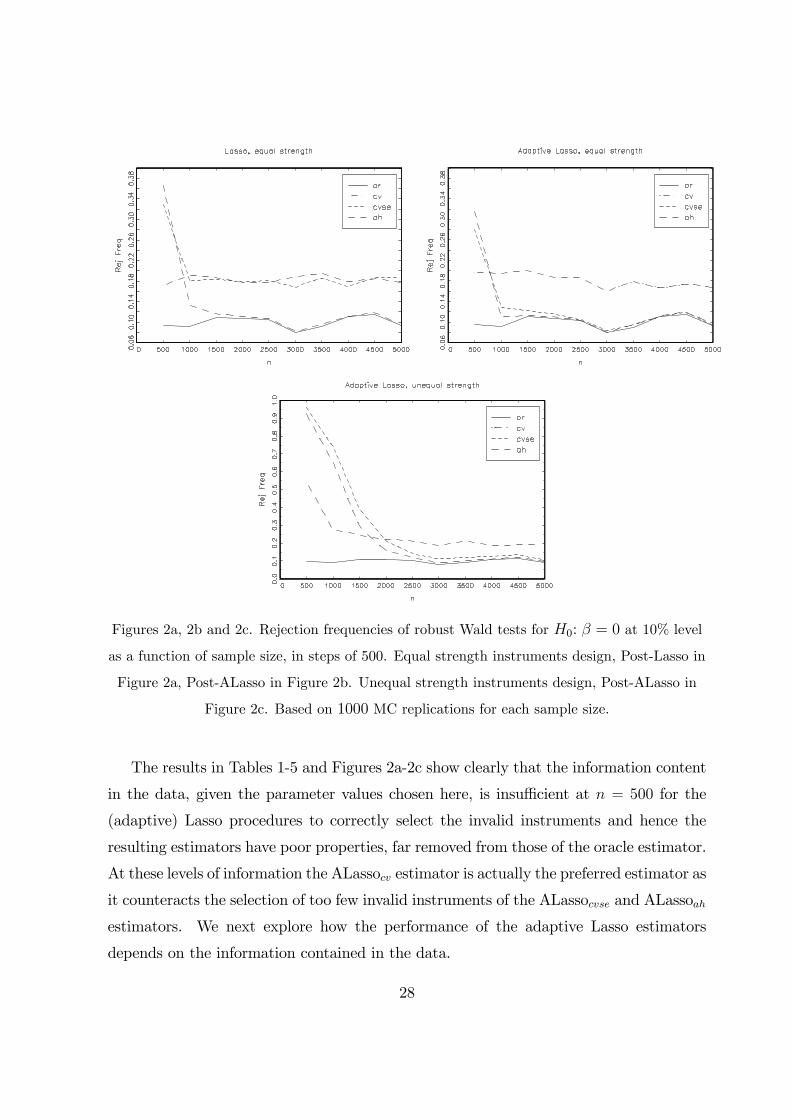
Figures 2a, 2b and 2c. Rejection frequencies of robust Wald tests for H�: β = 0 at 10% level

as a function of sample size, in steps of 500. Equal strength instruments design, Post-Lasso in

Figure 2a, Post-ALasso in Figure 2b. Unequal strength instruments design, Post-ALasso in

Figure 2c. Based on 1000 MC replications for each sample size.

The results in Tables 1-5 and Figures 2a-2c show clearly that the information content

in the data, given the parameter values chosen here, is insufficient at n = 500 for the

(adaptive) Lasso procedures to correctly select the invalid instruments and hence the

resulting estimators have poor properties, far removed from those of the oracle estimator.

At these levels of information the ALassocv estimator is actually the preferred estimator as

it counteracts the selection of too few invalid instruments of the ALassocvse and ALassoah

estimators. We next explore how the performance of the adaptive Lasso estimators

depends on the information contained in the data.

28

7.2 Information content

We distinguish two different measures of information in the IV Lasso selection problem.

First, as mentioned in Section 5, the information content for the estimation of β in the

oracle instrumental variables model is characterised by the concentration parameter µ�n,

Rothenberg (1984), which is here given by

µ�n =γ ′�Z

′�MZ�Z�γ�σ�v

.

µ�n is approximately equal to n (L− s) γ�� = 140 for the n = 500 cases above, which is

equivalent to a first-stage population F-test value for the null H� : γ� = 0 of nγ�� = 20.

This is a reasonably large value of the F-test, see Staiger and Stock (1997) and Stock

and Yogo (2005), which is reflected in the good properties of the oracle 2SLS estimator.

Clearly, though, the Lasso procedures do not perform well for the n = 500 case, especially

when γ� = 3γ�.

Note that the Wald test for H� : γ� = 0 is given by Wγ� =γ′��

′���

��γ�σ�

and so µ�n is

the population counterpart of the Wald test. The corresponding F-test is Wγ�/ (L− s).The weak instrument asymptotics of Staiger and Stock (1997) is obtained by considering

γ� in a neighbourhood of 0, as γ� = cγ�/√n, with cγ� a vector of constants. The

information content µ�n does then not increase with the sample size and converges to µ�c =

c′γ�Q��cγ�/σ�v as n → ∞. The oracle 2SLS estimator is in that case not consistent and

converges to a random variable with expected value different from β, with the difference

larger for smaller values of µ�c .

Second, a measure of information for the Lasso selection is the (squared) Signal to

Noise Ratio (SNR), see e.g. Bühlmann and Van de Geer (2011, p. 25), defined as

η� =α′Cα

σ�ε=α′�C��α�σ�ε

,

where, as before, C = plim(�nZ′Z

)and C�� = plim

(�nZ′�Z�

). From the proof of Propo-

sition 1 in the Appendix we obtain

α′�C��α� = α′�Q��α� −

(γ ′�Q��α� + γ′�Q��α�)

�

γ ′�Q��γ� + 2γ′�Q��γ� + γ

′�Q��γ�

. (25)

It follows from (25) that if we multiply α� by a factor m, η� gets multiplied by m�

whereas multiplying γ by a factor m does not affect the value of η�.

29

For the Monte Carlo design above, with σ�ε = 1, it follows that

η� = sa� − (saγ�)�

sγ�� + (L− s) γ��

=(L− s) a�(γ�γ�

)�+ L−s

s

,

and so the SNR is here directly influenced by the relative value |γ�/γ�|, with an increase inthis value decreasing the value of η�. For the unequal strength design above, η� = 0.0247,

and for the equal strength design it is η� = 0.0840. As Zou (2006) indicated, the smaller

value of the SNR in the unequal design explains the poorer performance of the adaptive

Lasso estimators for a given sample size, as depicted in Figures 2b and 2c.

The concentration parameter equivalent of η� is

η�n =α′�Z

′�Z�α�σ�ε

,

which is the population counterpart of the Wald test for H� : α� = 0 based on the oracle

2SLS estimator

Wα� =α′�,orZ

′�Z�α�,or

σ�ε,or.

In order to illustrate the performance of the adaptive Lasso estimator in relation to

the value of η�n, Table 6 shows the rejection frequencies at the 10% level of the robust

Wald tests Wβ,r based on the oracle and post-ALassoah estimators, for the n = 500

unequal strength case as in Section 5.2, but increasing α by a multiplicative factor m =√1,√3, ...,

√9, and hence increasing η� and η�n (approximately) by a multiplicative factor

m�. At m� = 9, the post-ALassoah estimator again behaves like the oracle estimator.

The mean of η�n is 116 there, with the associated population F-test statistic equal to

η�n/3 = 38.7. Increasing the value of a, whilst keeping γ constant, increases of course the

bias of the naive 2SLS estimator as is clear from (21).

Increasing γ� and γ� by the same multiplicative factor whilst keeping a and the

sample size constant does not alter η� and η�n, and does not lead to an improvement of

the performance of the Wald test Wβ,r, as confirmed by the results in Table 6. The bias

of the naive 2SLS estimator decreases here with increasing values of m.

30

Table 6. Rejection frequencies of Wβ,r at 10% level, varying α or γm�

α×m 1 3 5 7 9post-ALassoah 0.9300 0.3130 0.1350 0.1100 0.1070Oracle 0.1020 0.1030 0.1020 0.1010 0.1040η�n (mean) 12.90 38.69 64.51 90.31 116.13γ ×mpost-ALassoah 0.9300 0.9270 0.9340 0.9360 0.9360Oracle 0.1020 0.0960 0.0980 0.1010 0.0980η�n (mean) 12.90 12.51 12.43 12.39 12.37Notes: n = 500, same design as in Tables 3 and 5 when m = 1, 1000 MC replications

Multiplying both γ andα by a factorm increases both µ�n and η�n by a factorm

�, which

is then similar to an increase in the sample size n by a factor m�. For example, Table

7 displays estimation results for the unequal strength design for n = 500, multiplying a,

γ� and γ� by m =√20. The estimation results are very similar to those for n = 10, 000

as reported in Tables 3 and 5.

Table 7. Estimation results for β; n = 500, γ� = 3γ�, a = γ� = 0.8944av. # instr freq. all s

selected as invalid invalid instrβ bias std dev rmse mad [min, max] selected2SLS 0.2650 0.0106 0.2652 0.2651 0 02SLS or -0.0002 0.0191 0.0191 0.0128 3 1βm 0.0272 0.0229 0.0356 0.0267Post-ALassocvse 0.0003 0.0194 0.0194 0.0132 3.02 [3,5] 1Post-ALassoah 0.0000 0.0192 0.0192 0.0130 3.02 [3,5] 1Notes: Results from 1000 MC replications; L = 10, s = 3, β = 0, ρ = 0.25

Whilst η�n does seem to provide information content for the Lasso selection, its value

itself does not convey the same information about the performance of the adaptive Lasso

estimators as µ�n does for the oracle 2SLS estimator. We first illustrate this with an

example where the coefficients in α� take different values. In this case, the performance of

the Lasso estimator is driven by how well it does in selecting the variable with the smallest

value |αj|, j = 1, ..., s. If we for example change α� to α� =(0.1 0.2 0.2063

)′, we

get the same value of η� = 0.0247 in the unequal strength design, but as Figure 3 shows,

31

a much larger sample size is needed for the inference based on the post-ALassocvse and

post-ALassoah estimators to be similar to that of the oracle estimator, due to the presence

of the smaller coefficient α� = 0.1.

Figure 3. Rejection frequencies of robust Wald tests for H�: β = 0 at 10% level as a function

of sample size, in steps of 500. Unequal strength instruments design, Post-ALasso,

α�=(0.1 0.2 0.2063

). Based on 1000 MC replications for each sample size.

In order to convey this information, instead of η�n related to the Wald test on α�, we

compute the η�n,j related to the individual Wald tests for H� : αj = 0 in the oracle model,

resulting in

η�n,j =α�j

(Z′�,.jM�����

Z�,.j

)

σ�ε,

for j = 1, ..s, where Z�,.j is the j-th column of Z� and Z��j� are the other s−1 columns ofZ�. With η�j = plim

(�nη�n,j

), it follows for the specific design above with α� = α�/2 that

η�� =� η��, and η

�n,� ≈ �

η�n,�, conveying the smaller amount of information. As shown in

Figure 3, at, and from, n = 8500 the behaviour of the post-ALassoah estimator is close to

that of the oracle estimator with the rejection frequencies of Wβ,r at the 10% level equal

to 0.1000 for the post-ALassoah estimator and 0.0920 for the oracle estimator. The mean

value of η�n at n = 8500 is equal to 220, whereas those of η�n,�, η

�n,� and η

�n,� are equal to

37, 149, and 159 respectively. In comparison, for the unequal strength design results as

32

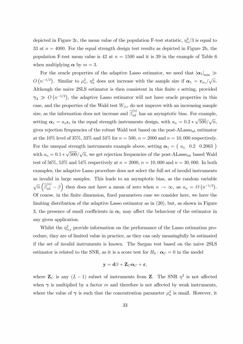
depicted in Figure 2c, the mean value of the population F-test statistic, η�n/3 is equal to

33 at n = 4000. For the equal strength design test results as depicted in Figure 2b, the

population F-test mean value is 42 at n = 1500 and it is 39 in the example of Table 6

when multiplying α by m = 3.

For the oracle properties of the adaptive Lasso estimator, we need that |α�|��� �O(n−�/�

). Similar to µ�n, η

�n does not increase with the sample size if α� = cα�/

√n.

Although the naive 2SLS estimator is then consistent in this finite s setting, provided

γ� � O(n−�/�

), the adaptive Lasso estimator will not have oracle properties in this

case, and the properties of the Wald test Wβ,r do not improve with an increasing sample

size, as the information does not increase and β�n�

ad has an asymptotic bias. For example,

setting α� = anιs in the equal strength instruments design, with an = 0.2 ∗√500/

√n,

gives rejection frequencies of the robust Wald test based on the post-ALassoah estimator

at the 10% level of 35%, 33% and 34% for n = 500, n = 2000 and n = 10, 000 respectively.

For the unequal strength instruments example above, setting α� =(an 0.2 0.2063

)

with an = 0.1 ∗√500/

√n, we get rejection frequencies of the post-ALassoah based Wald

test of 56%, 53% and 54% respectively at n = 2000, n = 10, 000 and n = 30, 000. In both

examples, the adaptive Lasso procedure does not select the full set of invalid instruments

as invalid in large samples. This leads to an asymptotic bias, as the random variable√n(β�n�

ad − β)then does not have a mean of zero when n → ∞, as an = O

(n−�/�

).

Of course, in the finite dimension, fixed parameters case we consider here, we have the

limiting distribution of the adaptive Lasso estimator as in (20), but, as shown in Figure

3, the presence of small coefficients in α� may affect the behaviour of the estimator in

any given application.

Whilst the η�n,j provide information on the performance of the Lasso estimation pro-

cedure, they are of limited value in practice, as they can only meaningfully be estimated

if the set of invalid instruments is known. The Sargan test based on the naive 2SLS

estimator is related to the SNR, as it is a score test for H� : αC = 0 in the model

y = dβ + ZCαC + ε,

where ZC is any (L− 1) subset of instruments from Z. The SNR η� is not affected

when γ is multiplied by a factor m and therefore is not affected by weak instruments,

where the value of γ is such that the concentration parameter µ�n is small. However, it

33

is well known that weak instruments decreases the power of the Sargan/Hansen test, see

Staiger and Stock (1997) and Kitamura (2006), which would then affect the behaviour

of the post-ALassoah estimator, as the decrease in power will result in less instruments

selected as invalid. This is illustrated in Table 8, which presents results for the unequal

instrument, large a design as in Table 6, for n = 500, a = 0.6, γ� = 0.6, γ� = 0.2,

and γ multiplied by a factor 1/m for m� = 1, 3, ..., 9. We present results here for the

median bias, as the variability of the estimators increases substantially for larger values

of m. For increasing value of m, the number of selected invalid instruments decreases for

the ALassoah estimator, whilst that of the ALassocvse actually increases, and the median

bias of the ALassoah estimator increases relative to that of the ALassocvse estimator.

Increasing the p-value for the Hansen test decreases the bias of the ALassoah estimator.

For example, for m = 3, setting the p-value to 0.2 instead of 0.016 increases the average

number of selected instruments as invalid to 3.13 and reduces the median bias of the

estimator to 0.1022. The post-ALassoah estimator is, however, a much noisier estimator

here with a standard deviation of 0.66 compared to 0.35 for the post-ALassocvse estimator

and 0.21 for the oracle 2SLS estimator.

Table 8. Median bias for 2SLS estimators of β; L = 10, s = 3m�

γ × (1/m) 1 3 5 7 92SLS 0.7883 1.3311 1.6778 1.9464 2.15702SLS or 0.0087 0.0344 0.0504 0.0666 0.0740post-ALassocvse 0.0138 0.0410 0.0632 0.0899 0.0992# Inv Inst 3.07 3.10 3.17 3.26 3.31post-ALassoah 0.0103 0.0348 0.0556 0.0920 0.1257# Inv Inst 3.01 3.01 2.88 2.61 2.37µ�n 678.51 225.66 136.40 96.86 75.14η�n 116.13 127.44 135.88 146.86 157.21Notes: n = 500, a = 0.6, γ�= 3γ�, γ�= 0.2/m, 1000 MC replications

Even when all the coefficients in α� are the same, the value of η�n itself is not sufficient

as a guide to the performance of the adaptive Lasso estimator. As illustrated above,

within the same design, a larger value for η�n was associated with a better performance

of the adaptive Lasso estimator. However, across designs this may not be the case.

For example, we show in Appendix A.2 that introducing correlation to the instruments,

34

whilst keeping µ� = plim (µ�n/n) and η� constant, requires larger samples and hence

larger values of η�n than in the uncorrelated instruments designs, for the performance of

the robust Wald test Wβ,r based on the post-ALasso estimators to be close to that based

on the oracle estimator.

Assumption 3 states that the instruments are relevant in the sense that γj �= 0, forj = 1, ..., L. If this assumption is relaxed and some of the γj are equal to 0, then the

instruments are potentially invalid for two reasons as the relevance and/or exclusion

condition may fail. If γj = 0, then |πj| =∣∣(βγj + αj

)/γj∣∣ is either ∞ for instruments

with αj �= 0, or ill defined as β + 0/0. The median and adaptive Lasso estimators stillhave the properties as stated in Section 4 if we make the assumption that more than

50% of the instruments are valid and relevant. Another remedy to a relevance problem

would be to do an initial selection of the instruments by for example a Lasso selection

in the model d = Zγ + v, with the identification condition then that less than 50% of

the selected (i.e. sufficiently strong) instruments are invalid. This is the approach taken

by Guo et al. (2016), who then proceed to select the invalid instruments by a pairwise

comparison of the πj.

8 The Effect of BMI on Diastolic Blood PressureUsing Genetic Markers as Instruments

We use data on 105, 276 individuals from the UK Biobank and investigate the effect of

BMI on diastolic blood pressure (DBP). See Sudlow et al. (2015) for further information

on the UK Biobank. We use 96 single nucleotide polymorphisms (SNPs) as instruments

for BMI as identified in independent GWAS studies, see Locke et al. (2015).

With Mendelian randomisation studies the SNPs used as potential instruments can

be invalid for various reasons, such as linkage disequilibrium, population stratification

and horizontal pleiotropy, see e.g. von Hinke et al. (2016) or Davey Smith and Hemani

(2014). For example, a SNP has pleiotropic effects if it not only affects the exposure but

also has a direct effect on the outcome. Whilst we guard against population stratification

by considering only white European origin individuals in our data, the use of the Lasso

methods can be extremely useful here to identify the SNPs with direct effects on the

outcome and to estimate the causal effect of BMI on diastolic blood pressure taking

35

account of this.

Because of skewness, we log-transformed both BMI and DBP. The linear model spec-

ification includes age, age� and sex, together with 15 principal components of the genetic

relatedness matrix as additional explanatory variables. Table 9 presents the estimation

results for the causal effect parameter, which is here the percentage change in DBP due

to a 1% change in BMI. As p-value for the Hansen test based procedures we take again

0.1/ ln (n) = 0.0086.

The OLS estimate of the causal parameter is equal to 0.206 (s.e. 0.003), whereas the

2SLS estimate treating all 96 instruments as valid is much smaller at 0.087 (s.e. 0.016),

with a 95% confidence interval of [0.056,0.118]. The J-test, however, rejects the null

that all the instruments are valid. The Lassocv estimator identifies a large number of

56 instruments as invalid and the Lassocv estimate is equal to 0.126, the post-Lassocv

estimate equal to 0.145. The Lassocvse procedure identifies 20 instruments as invalid

and the Lassocvse estimate is equal to 0.111. The post-Lassocvse estimate is larger and

equal to 0.142, which is in line with our findings above that the Lasso estimator is biased

towards the 2SLS estimator that treats all instruments as valid due to shrinkage. The

post-Lassoah procedure selects a subset of 12 instruments as invalid, and the post-Lassoah

parameter estimate is equal to 0.122.

The median estimate βm is equal to 0.148. Using this estimate for the adaptive

Lasso results in the cv method selecting 54 instruments as invalid and the cvse method

selecting 17 instruments as invalid. The adaptive Lassoah method selects a subset of 11

instruments as invalid. The post-ALassocv, post-ALassocvse and post-ALassoah estimates

are equal to 0.161, 0.151 and 0.163 respectively, with the 95% confidence intervals of the

post-ALassocvse and post-ALassoah estimators given by [0.113,0.189] and [0.127,0.198]

respectively. These results indicate that the OLS estimator is less confounded than

suggested by the 2SLS estimation results using all 96 instruments as valid instruments.

The strongest potential instrument is the FTO SNP. For all Lasso estimators in Table

9 it is selected as an invalid instrument. The value for πFTO = −0.009, i.e. negative,which is contrary to the direction of the found causal effect.

36

Table 9. Estimation results, the effect of ln (BMI) on ln (DBP )estimate rob st err # instr p-value J-test

selected as invalid

OLS 0.206 0.0032SLS 0.087 0.016 0 0.0000

Lassocv 0.126 56Post-Lassocv 0.145 0.033 1.0000

Lassocvse 0.111 20Post-Lassocvse 0.142 0.020 0.6435Post-Lassoah 0.122 0.018 12 0.0123

median, βm 0.148ALassocv 0.158 54

Post-ALassocv 0.161 0.029 1.0000ALassocvse 0.131 17

Post-ALassocvse 0.151 0.019 0.4091Post-ALassoah 0.163 0.018 11 0.0102Notes: sample size n = 105, 276; L = 96

The F-test statistic for H� : γ� = 0 for the model resulting from the ALassoah

procedure is equal to 18.21 with the associated estimate of the concentration parameter

equal to 1547.81. The F-test result indicates that the 2SLS estimator may have some

many weak instruments bias, see Stock and Yogo (2005). However, the LIML (Limited

Information Maximum Likelihood) estimator in this model is very similar to the 2SLS

estimator and equal to 0.159 (s.e. 0.019), indicating that there is not a many weak

instruments problem here, see Davies et al. (2015).

9 Conclusions

Instrumental variables estimation is a well established procedure for the identification and

estimation of causal effects of exposures on outcomes where the observed relationships

are confounded by non-random selection of exposure. The main identifying assumption is

that the instruments satisfy the exclusion restriction, i.e. they only affect the outcomes

through their relationship with the exposure. In an important contribution, Kang et

al. (2016) show that the Lasso method for variable selection can be used to select invalid

37

instruments in linear IV models, even though there is no prior knowledge about which

instruments are valid.

We have shown here that, even under the sufficient condition for identification that

less than 50% of the instruments are invalid, the Lasso selection may select the valid

instruments as invalid if the invalid instruments are relatively strong, i.e. the case where

an invalid instrument explains more of the exposure variance than a valid instrument.

Consistent selection of invalid instruments also depends on the correlation structure of

the instruments.

We show that a median estimator is consistent when less than 50% of the instruments

are invalid, and its consistency does not depend on the relative strength of the instru-

ments or their correlation structure. This initial consistent estimator can be used for

the adaptive Lasso estimator of Zou (2006) and we show that it performs well for larger

sample sizes/information settings in our simulations. This adaptive Lasso estimator has

the same limiting distribution as the oracle 2SLS estimator, and solves the inconsistency

problem of the Lasso method when the relative strength of the invalid instruments is

such that the Lasso method selects the valid instruments as invalid.

Whilst less than 50% invalid instruments is a sufficient condition for identification,

in principle the parameters are identified if the valid instruments form the largest group.

Instruments form a group if they have the same estimate for the causal effect. Future

research will therefore focus on how to obtain consistent results when more than 50% of

the instruments are invalid, but the parameters are such that they are asymptotically

identified.

References

[1] Abadir, K.M., and J.R. Magnus, (2005), Matrix Algebra, Econometric Exercises 1,

Cambridge University Press, Cambridge.

[2] Andrews, D.W.K., (1999), Consistent Moment Selection Procedures for Generalized

Method of Moments Estimation, Econometrica 67, 543-564.

[3] Angrist, J.D., and A.B. Krueger, (1991), Does Compulsory School Attendance Affect

Schooling and Earnings?, Quarterly Journal of Economics 106, 979-1014.

38

[4] Bekker, P.A., (1994), Alternative Approximations to the Distributions of Instrumen-

tal Variable Estimators, Econometrica 62, 657-681.

[5] Belloni, A., D. Chen, V. Chernozhukov and C. Hansen, (2012), Sparse Models and

Methods for Optimal Instruments with an Application to Eminent Domain, Econo-

metrica 80, 2369-2429.

[6] Belloni, A. and V. Chernozhukov, (2013), Least squares after model selection in

high-dimensional sparse models, Bernoulli 19, 521-547.

[7] Belloni, A., V. Chernozhukov and C. Hansen, (2014), Inference on Treatment Effects

after Selection among High-Dimensional Controls, Review of Economic Studies 81,

608-650.

[8] Bowden, J., G.D. Smith, S. Burgess, (2015), Mendelian Randomization with In-

valid Instruments: Effect Estimation and Bias Detection through Egger Regression,

International Journal of Epidemiology 44, 512-525.

[9] Bühlmann, P. and S. van der Geer, (2011), Statistics for High-Dimensional Data.

Methods Theory and Applications. Springer Series in Statistics, Springer, Heidelberg.

[10] Burgess, S., D.S. Small and S.G. Thompson, (2015), A Review of Instrumental

Variable Estimators for Mendelian Randomization, Statistical Methods in Medical

Research, in Press.

[11] Cheng, X., Z. Liao, (2015), Select the Valid and Relevant Moments: An Information-

based LASSO for GMMwith ManyMoments, Journal of Econometrics 186, 443-464.

[12] Chernozhukov V., C. Hansen and M. Spindler, (2015), Post-Selection and Post-

Regularization Inference in Linear Models with Many Controls and Instruments,

American Economic Review 105, 486-490.

[13] Clarke, P.S. and F. Windmeijer, (2012), Instrumental Variable Estimators for Binary

Outcomes, Journal of the American Statistical Association 107, 1638-1652.

[14] Davey Smith, G. and G. Hemani, (2014), Mendelian randomization: genetic anchors

for causal inference in epidemiological studies. Human Molecular Genetics 23, R89-

R98.

39

[15] Davidson, R. and J.G. MacKinnon, (1993), Estimation and Inference in Economet-

rics, Oxford: Oxford University Press.

[16] Davies, N.M., S. von Hinke Kessler Scholder, H. Farbmacher, S. Burgess, F. Wind-

meijer and G. Davey Smith, (2015), The Many Weak Instruments Problem and

Mendelian Randomization, Statistics in Medicine 34, 454-468.

[17] Efron, B., T. Hastie, I. Johnstone and R. Tibshirani, (2004), Least Angle Regression,

The Annals of Statistics 32, 407-451.

[18] Greenland, S., (2000), An introduction to instrumental variables for epidemiologists,

International Journal of Epidemiology 29, 722-729.

[19] Guo, Z., H. Kang, T. Cai and D. Small, (2016), Confidence Intervals for Causal

Effects with Invalid Instruments using Two-Stage Hard Thresholding, arXiv:

1603.05224.

[20] Han, C., (2008), Detecting Invalid Instruments using L�-GMM, Economics Letters

101, 285-287.

[21] Hansen, C., J. Hausman and W.K. Newey, (2008), Estimation with Many Instru-

mental Variables, Journal of Business & Economic Statistics 26, 398-422.

[22] Hansen, L.P., (1982), Large Sample Properties of Generalized Method of Moments

Estimators, Econometrica 50, 1029-1054.

[23] Hastie, T., R. Tibshirani and J. Friedman, (2009), The Elements of Statistical Learn-

ing. Data Mining, Inference, and Prediction. Second Edition, Springer Series in Sta-

tistics. New York: Springer Science and Business Media.

[24] von Hinke, S., G. Davey Smith, D.A. Lawlor, C. Propper and F. Windmeijer, (2016),

Genetic Markers as Instrumental Variables, Journal of Health Economics 45, 131-

148.

[25] Imbens, G.W., (2014), Instrumental Variables: An Econometrician’s Perspective,

Statistical Science 29, 323-358.

40

[26] Kang, H., A. Zhang, T.T. Cai and D.S. Small, (2016), Instrumental Variables Esti-

mation with some Invalid Instruments and its Application to Mendelian Random-

ization, Journal of the American Statistical Association 111, 132-144.

[27] Kitamura, Y. (2006), Specification Tests with Instrumental Variables and Rank

Deficiency. In D. Corbae, S. Durlauf, & B. Hansen (Eds.), Econometric Theory and

Practice: Frontiers of Analysis and Applied Research, 59-81. Cambridge: Cambridge

University Press.

[28] Kolesar, M., R. Chetty, J. Friedman, E. Glaeser, G.W. Imbens, (2015), Identification

and Inference with Many Invalid Instruments, Journal of Business and Economic

Statistics 33, 474-484.

[29] Lawlor, D.A., R.M. Harbord, J.A.C. Sterne,N. Timpson and G. Davey Smith, (2008),

Mendelian Randomization: Using Genes as Instruments for Making Causal Infer-

ences in Epidemiology, Statistics in Medicine 27, 1133-1163.

[30] Liao, Z., (2013), Adaptive GMM Shrinkage Estimation with Consistent Moment

Selection, Econometric Theory 29, 857-904.

[31] Lin, W., R. Feng, H. Li, (2015), Regularization Methods for High-Dimensional In-

strumental Variables Regression With an Application to Genetical Genomics, Jour-

nal of the American Statistical Association 110, 270-288.

[32] Locke, A.E., et al., (2015), Genetic Studies of Body Mass Index Yield New Insights

for Obesity Biology. Nature 518, 197—206.

[33] Meinshausen, N. and P. Bühlmann, (2006), High-dimensional graphs and variable

selection with the Lasso, Annals of Statistics 34, 1436-1462.

[34] Newey, W.K. and F. Windmeijer, (2009), Generalized Methods of Moments with

Many Weak Moment Conditions, Econometrica 77, 687-719.

[35] Rothenberg, T.J., (1984), Approximating the Distributions of Econometric Estima-

tors and Test Statistics. In Z. Griliches and M.D. Intriligator (Eds.), Handbook of

Econometrics, Volume 2, 881-935. Amsterdam: North Holland.

41

[36] Sargan, J. D., (1958), The Estimation of Economic Relationships Using Instrumental

Variables. Econometrica 26, 393—415.

[37] Staiger, D. and J.H. Stock, (1997), Instrumental Variables Regression with Weak

Instruments, Econometrica 65, 557-586.

[38] Stock, J.H. and M. Yogo, (2005), Testing for Weak Instruments in Linear IV Re-

gression. In D.W.K. Andrews and J.H. Stock (Eds.), Identification and Inference for

Econometric Models, Essays in Honor of Thomas Rothenberg, 80-108. New York:

Cambridge University Press.

[39] Sudlow, C., J. Gallacher, N. Allen, V. Beral, P. Burton, J. Danesh et al., (2015),

UK Biobank: An Open Access Resource for Identifying the Causes of a Wide Range

of Complex Diseases of Middle and Old Age. PLoS Med 12: e1001779.

[40] Wainwright M.J., (2009), Sharp Thresholds for High-Dimensional and Noisy Sparsity

Recovery Using ��-Constrained Quadratic Programming (Lasso), IEEE Transactions

on Information Theory 55, 2183-2202.

[41] Zhao, P. and B. Yu, (2006), On Model Selection Consistency of Lasso, Journal of

Machine Learning Research 7, 2541-2563.

[42] Zou, H., (2006), The Adaptive Lasso and Its Oracle Properties, Journal of the

American Statistical Association 101, 1418-1429.

42

A Appendix

A.1 Proof of Proposition 1

Lemma 1 For nonsingular r × r matrix H and r-vector h, if h′H−�h �= 1, then

(H− hh′)−� = H−� +1

1− h′H−�hH−�hh′H−� (26)

and so

h′ (H− hh′)−� =

(1 +

h′H−�h

1− h′H−�h

)h′H−�

=1

1− h′H−�hh′H−�, (27)

Proof. See Abadir and Magnus (2005, page 87).

From the definitions in Section 3, we have

plim

(1

nZ′�Z�

)= Q�� − (Q��γ� +Q

′��γ�) (γ

′Qγ)−�(γ ′�Q�� + γ

′�Q��)

plim

(1

nZ′�Z�

)= Q�� − (Q��γ� +Q��γ�) (γ

′Qγ)−�(γ ′�Q�� + γ

′�Q��) .

Hence

C��C−��� = plim

(1

nZ′�Z�

)(plim

(1

nZ′�Z�

))−�

= ((γ ′Qγ)Q�� − (Q��γ� +Q��γ�) (γ′�Q�� + γ

′�Q��)) (28)

((γ ′Qγ)Q�� − (Q��γ� +Q′��γ�) (γ

′�Q�� + γ

′�Q��))

−�.

Let η = (Q��γ� +Q′��γ�). From (27), we get

η′ ((γ ′Qγ)Q�� − ηη′)−� =1

1− η′Q−��� η/γ

′Qγη′Q−�

�� /γ′Qγ

=1

γ ′Qγ − η′Q−��� η

η′Q−��� . (29)

Using (26),

(γ ′Qγ)Q�� ((γ′Qγ)Q�� − ηη′)−�

= Q��Q−��� + (γ

′Qγ)Q��1

1− η′Q−��� η/γ

′QγQ−��� ηη

′Q−��� / (γ

′Qγ)�

= Q��Q−��� +Q��Q

−��� η

1

γ ′Qγ − η′Q−��� η

η′Q−��� . (30)

43

Hence, combining (28), (29) and (30),

C��C−��� = Q��Q

−��� +

(Q��Q

−��� η − (Q��γ� +Q��γ�)

) 1

γ ′Qγ − η′Q−��� η

η′Q−��� . (31)

As

γ ′Qγ = γ ′�Q��γ� + 2γ′�Q

′��γ� + γ

′�Q��γ�

η′Q−��� η = γ ′�Q��γ� + 2γ

′�Q

′��γ� + γ

′�Q��Q

−���Q

′��γ�,

it follows that

γ ′Qγ − η′Q−��� η = γ

′�

(Q�� −Q��Q

−���Q

′��

)γ�. (32)

Further,

Q−��� η = γ� +Q

−���Q

′��γ� (33)

Q��Q−��� η − (Q��γ� +Q��γ�) =

(Q��Q

−���Q

′�� −Q��

)γ�. (34)

Combining (31), (32), (33) and (34), the result follows that

C��C−��� = Q��Q

−��� −

(Q�� −Q��Q

−���Q

′��

)γ�

γ ′� + γ′�Q��Q

−���

γ ′�(Q�� −Q��Q

−���Q

′��

)γ�.

A.2 Monte Carlo results for correlated instruments

Figures 4a-4c below show the rejection frequencies of the robust Wald test Wβ,r as in

Figures 2a-2c for equal and unequal strength instruments, but where the instruments are

correlated and distributed as follows

Zi. ∼ N (0,Σ) ,

with the elements of Σ given by

Σr,k = ω|r−k|

and ω = 0.5.

As in the designs of Figures 2a-2c, α� = aιs, γ� = γ�ιs, γ� = γ�ιL−s, L = 10, s = 3

and for the unequal strength design γ� = 3γ�. We set the parameters a and γ� such

that µ� = plim (µ�n/n) and η� are equal to those of the designs for Figures 2a-2c. This

44

results in γ� = 0.1321 for both designs, a = 0.1552 in the equal instruments design, and

a = 0.1448 in the unequal instruments design.

As the figures show, a larger sample size n is needed here for a performance of the

Wald test Wβ,r similar to that of the uncorrelated instruments designs.

Figures 4a, 4b and 4c. Rejection frequencies of robust Wald tests for H�: β = 0 at 10% level

as a function of sample size, in steps of 500. Correlated instruments, equal strength

instruments design, Post-Lasso in Figure 4a, Post-ALasso in Figure 4b. Unequal strength

instruments design, Post-ALasso in Figure 4c. Based on 1000 MC replications for each sample

size.

45