Embed Size (px)
Citation preview
DiscreteInferenceandLearningLecture1
MVA2017–2018
h;p://thoth.inrialpes.fr/~alahari/disinflearn
SlidesbasedonmaterialfromStephenGould,PushmeetKohli,NikosKomodakis,M.PawanKumar,CarstenRother
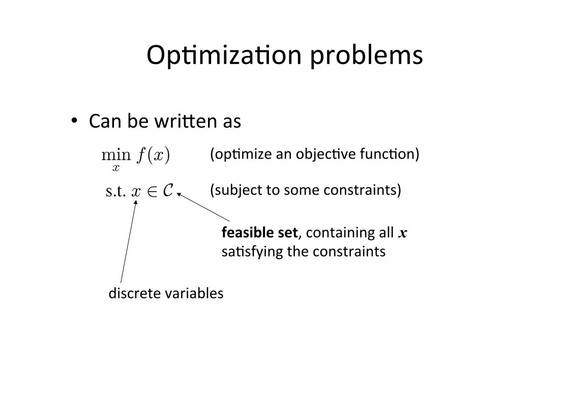
OpQmizaQonproblems
• Canbewri;enas(opQmizeanobjecQvefuncQon)
(subjecttosomeconstraints)
feasibleset,containingall x saQsfyingtheconstraints
discretevariables

OpQmizaQonproblems
• Canbewri;enas
• Twomainproblemsinthiscontext– OpQmizetheobjecQve(inference)– Learntheparametersoff(learning)
(opQmizeanobjecQvefuncQon)
(subjecttosomeconstraints)
OpQmizaQonproblems
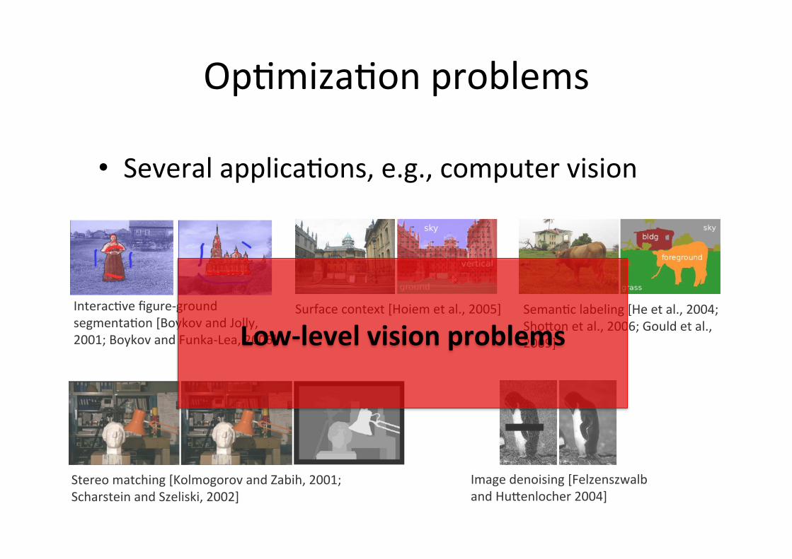
• SeveralapplicaQons,e.g.,computervision
InteracQvefigure-groundsegmentaQon[BoykovandJolly,2001;BoykovandFunka-Lea,2006]
Surfacecontext[Hoiemetal.,2005] SemanQclabeling[Heetal.,2004;Sho;onetal.,2006;Gouldetal.,2009]
Stereomatching[KolmogorovandZabih,2001;ScharsteinandSzeliski,2002]
Imagedenoising[FelzenszwalbandHu;enlocher2004]
Low-levelvisionproblems
OpQmizaQonproblems
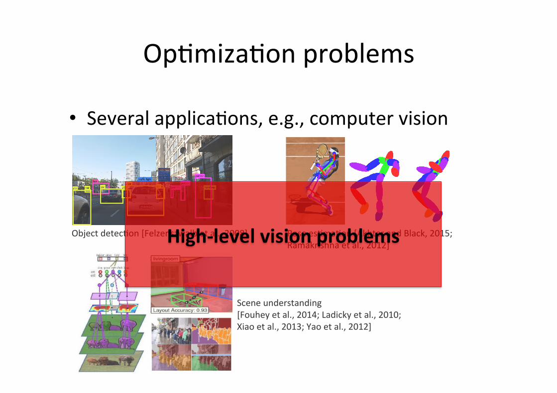
• SeveralapplicaQons,e.g.,computervision
ObjectdetecQon[Felzenszwalbetal.,2008] PoseesQmaQon[AkhterandBlack,2015;Ramakrishnaetal.,2012]
Sceneunderstanding[Fouheyetal.,2014;Ladickyetal.,2010;Xiaoetal.,2013;Yaoetal.,2012]
High-levelvisionproblems

OpQmizaQonproblems
• SeveralapplicaQons,e.g.,medicalimaging
OpQmizaQonproblems
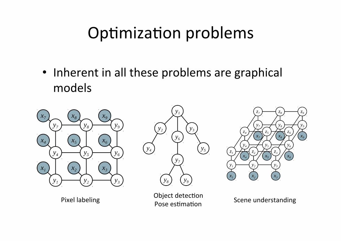
• Inherentinalltheseproblemsaregraphicalmodels
Pixellabeling ObjectdetecQonPoseesQmaQon Sceneunderstanding
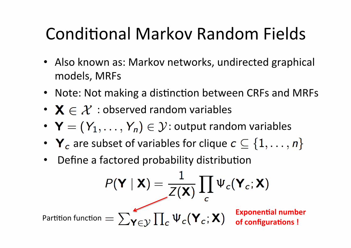
CondiQonalMarkovRandomFields• Alsoknownas:Markovnetworks,undirectedgraphicalmodels,MRFs
• Note:NotmakingadisQncQonbetweenCRFsandMRFs• :observedrandomvariables• :outputrandomvariables• aresubsetofvariablesforclique• DefineafactoredprobabilitydistribuQon
ParQQonfuncQonExponen9alnumberofconfigura9ons!
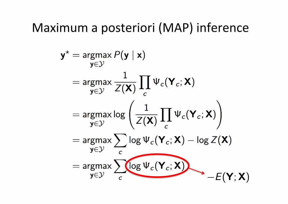
Maximumaposteriori(MAP)inference

Maximumaposteriori(MAP)inference
MAPinferenceóEnergyminimizaQon
TheenergyfuncQoniswhere CliquepotenQal
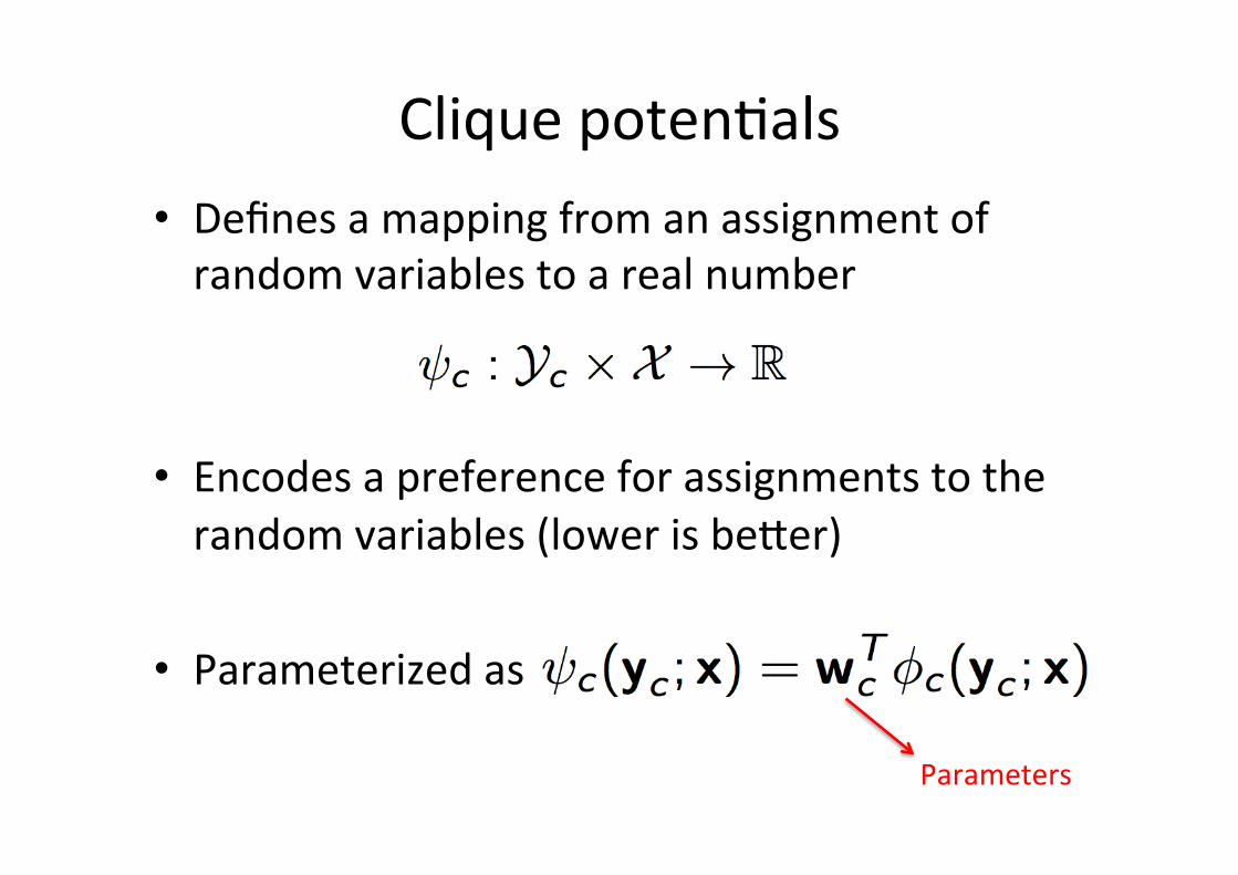
CliquepotenQals• Definesamappingfromanassignmentofrandomvariablestoarealnumber
• Encodesapreferenceforassignmentstotherandomvariables(lowerisbe;er)
• Parameterizedas
Parameters
CliquepotenQals
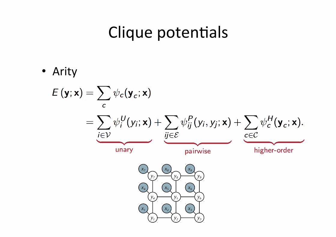
• Arity

CliquepotenQals
• Arity
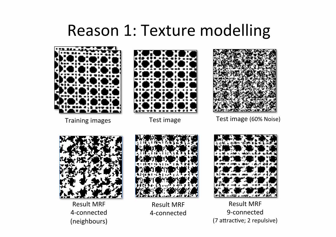
Reason1:Texturemodelling
Testimage Testimage(60%Noise)Trainingimages
ResultMRF9-connected
(7a;racQve;2repulsive)
ResultMRF4-connected
ResultMRF4-connected(neighbours)
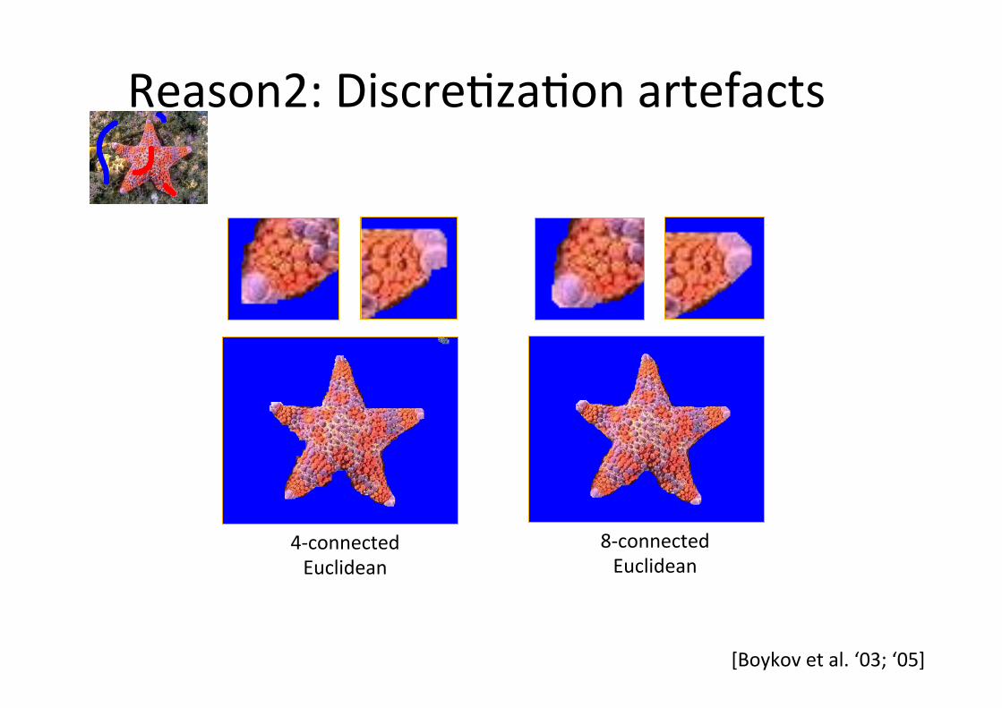
Reason2:DiscreQzaQonartefacts
4-connectedEuclidean
8-connectedEuclidean
[Boykovetal.‘03;‘05]
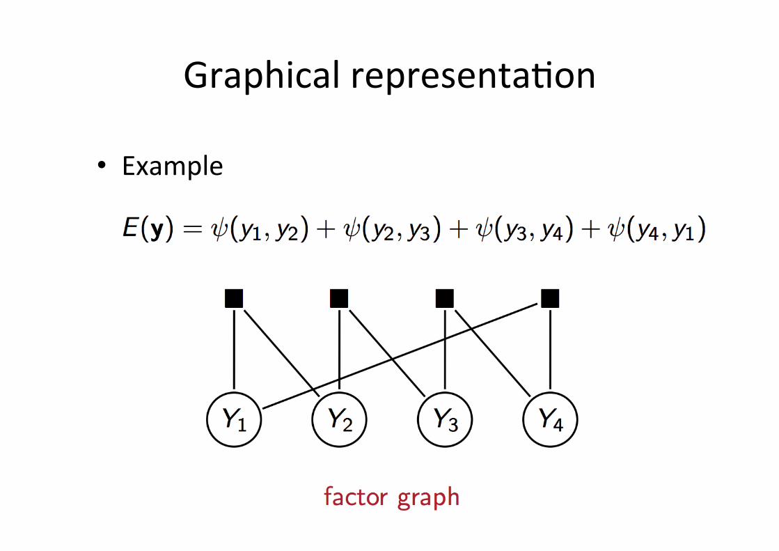
GraphicalrepresentaQon
• Example
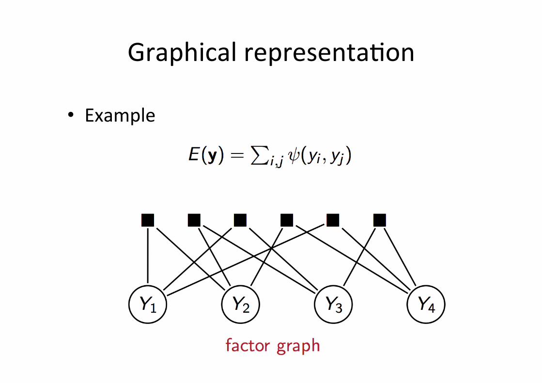
GraphicalrepresentaQon
• Example
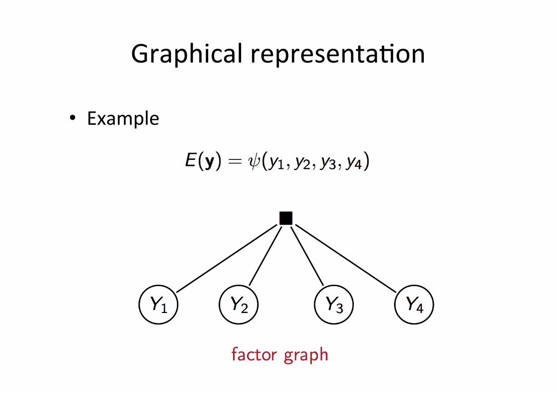
GraphicalrepresentaQon
• Example

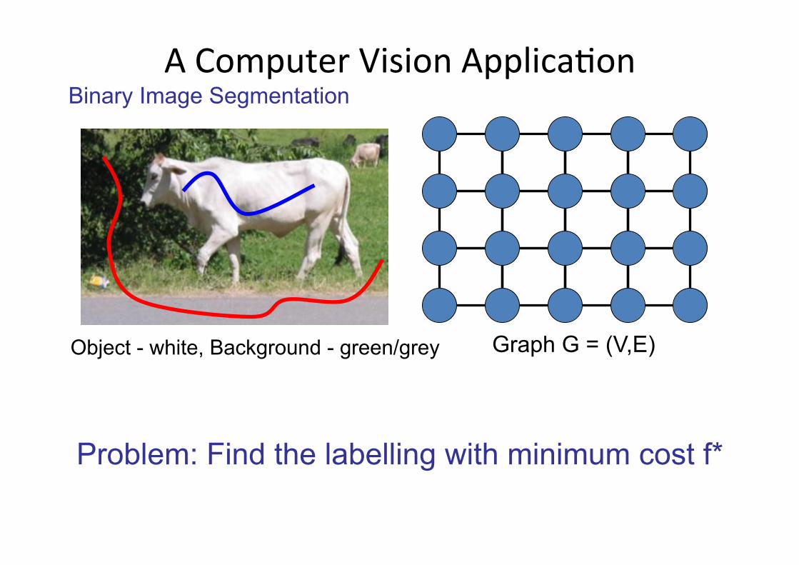
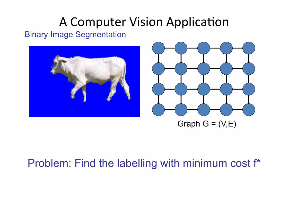
AComputerVisionApplicaQonBinary Image Segmentation
How ?
Cost function Models our knowledge about natural images
Optimize cost function to obtain the segmentation
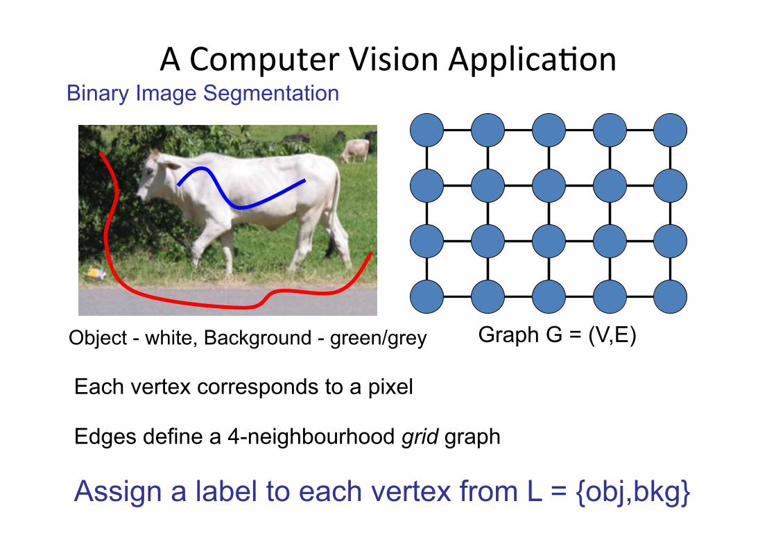
Object - white, Background - green/grey Graph G = (V,E)
Each vertex corresponds to a pixel
Edges define a 4-neighbourhood grid graph
Assign a label to each vertex from L = {obj,bkg}
AComputerVisionApplicaQonBinary Image Segmentation

Graph G = (V,E)
Cost of a labelling f : V ➔ L Per Vertex Cost
Cost of label ‘obj’ low Cost of label ‘bkg’ high
Object - white, Background - green/grey
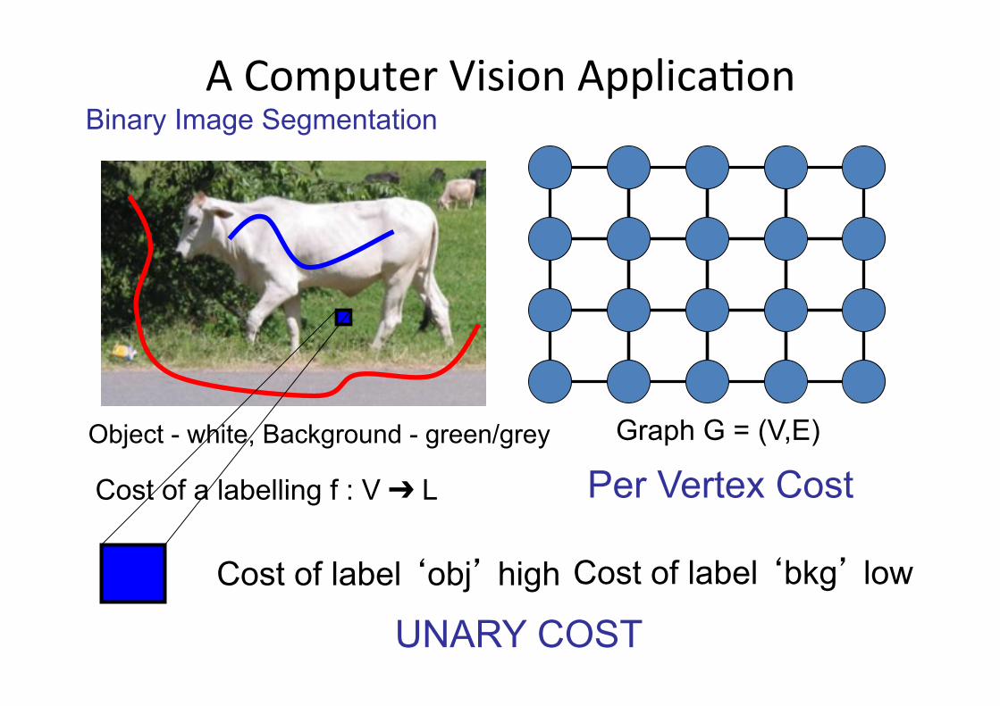
AComputerVisionApplicaQonBinary Image Segmentation
Graph G = (V,E)
Cost of a labelling f : V ➔ L
Cost of label ‘obj’ high Cost of label ‘bkg’ low
Per Vertex Cost
UNARY COST
Object - white, Background - green/grey
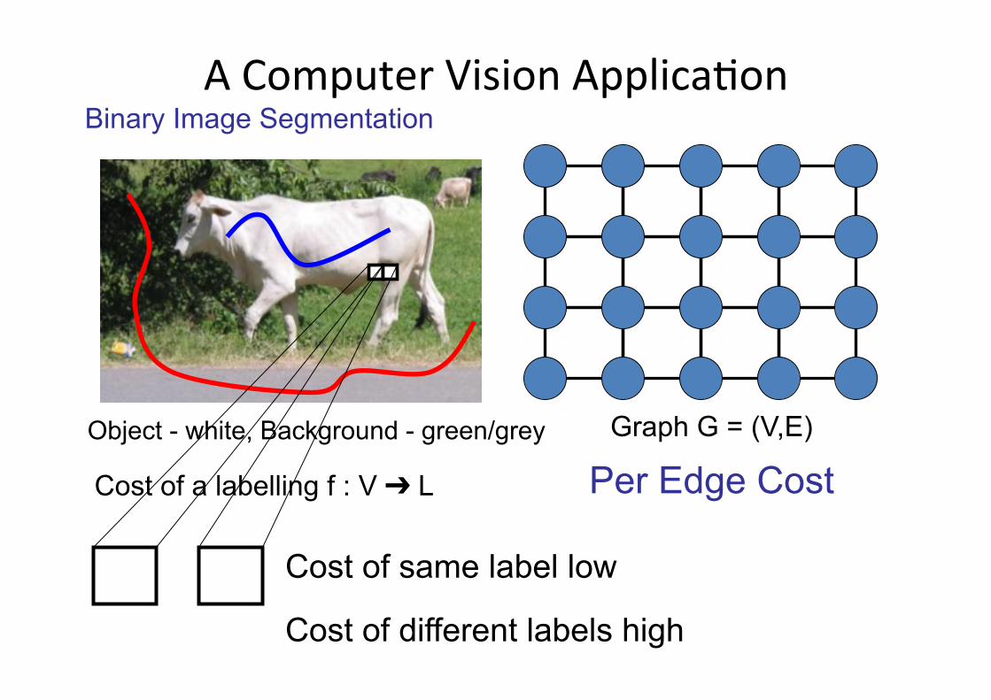
AComputerVisionApplicaQonBinary Image Segmentation
Graph G = (V,E)
Cost of a labelling f : V ➔ L Per Edge Cost
Cost of same label low
Cost of different labels high
Object - white, Background - green/grey
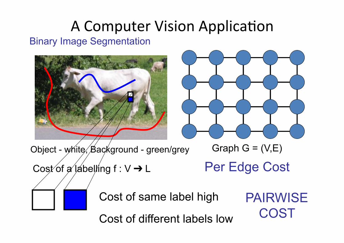
AComputerVisionApplicaQonBinary Image Segmentation
Graph G = (V,E)
Cost of a labelling f : V ➔ L
Cost of same label high
Per Edge Cost
PAIRWISE COST
Object - white, Background - green/grey
AComputerVisionApplicaQonBinary Image Segmentation
Cost of different labels low
Graph G = (V,E)
Problem: Find the labelling with minimum cost f*
Object - white, Background - green/grey
AComputerVisionApplicaQonBinary Image Segmentation
Graph G = (V,E)
Problem: Find the labelling with minimum cost f*
AComputerVisionApplicaQonBinary Image Segmentation
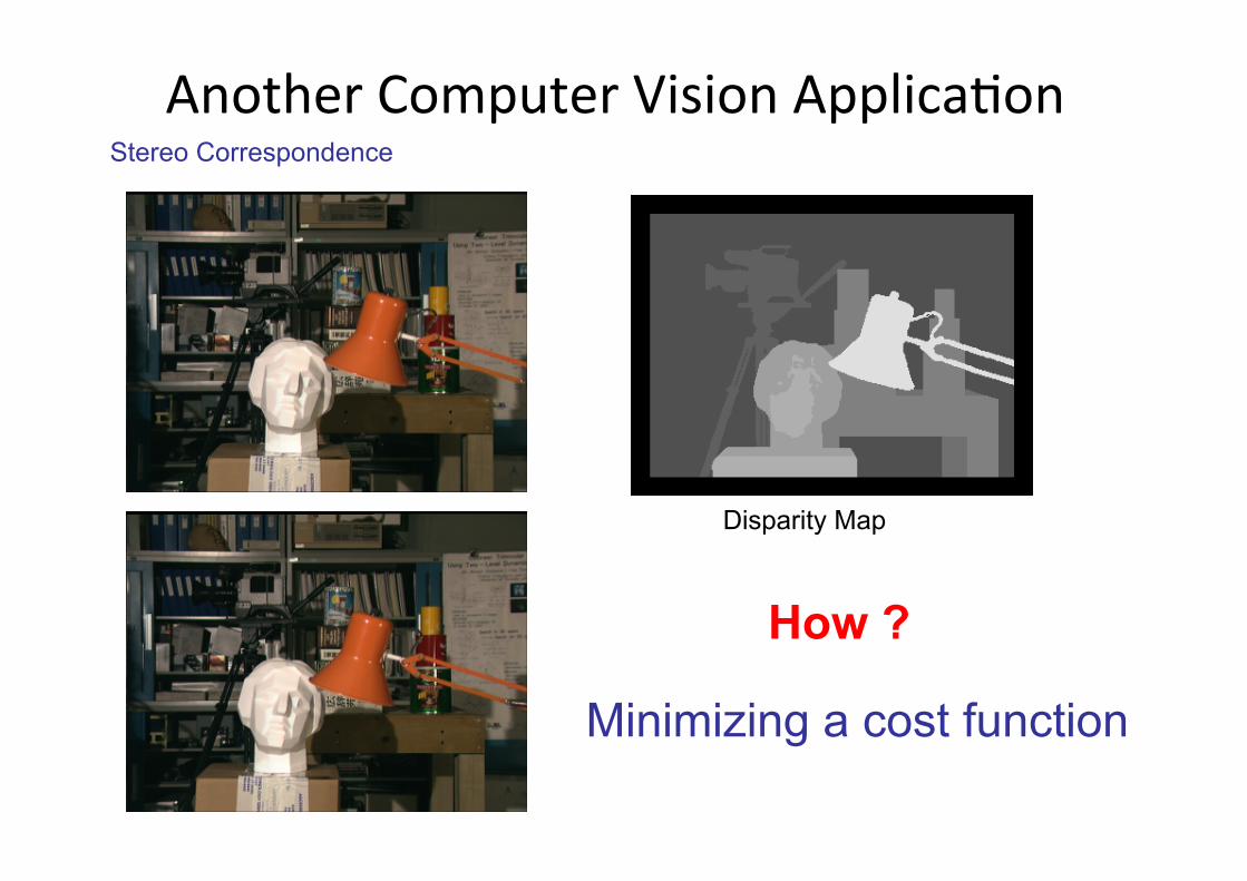
AnotherComputerVisionApplicaQonStereo Correspondence
Disparity Map
How ?
Minimizing a cost function
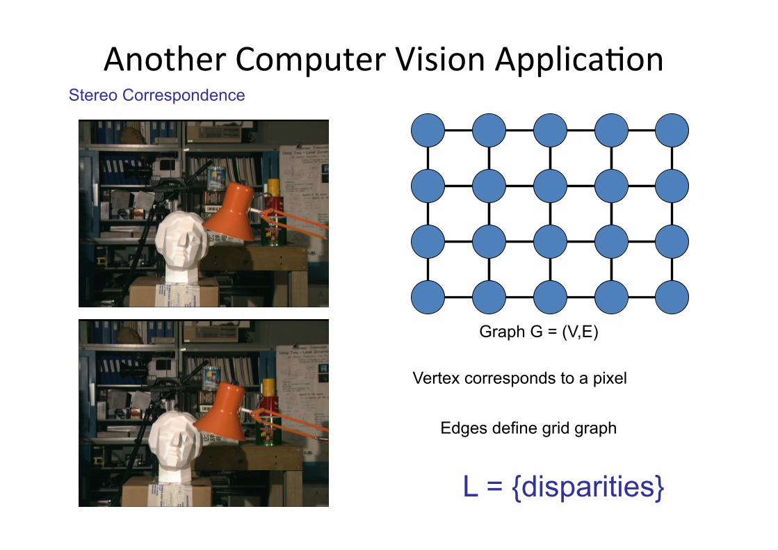
AnotherComputerVisionApplicaQonStereo Correspondence
Graph G = (V,E)
Vertex corresponds to a pixel
Edges define grid graph
L = {disparities}
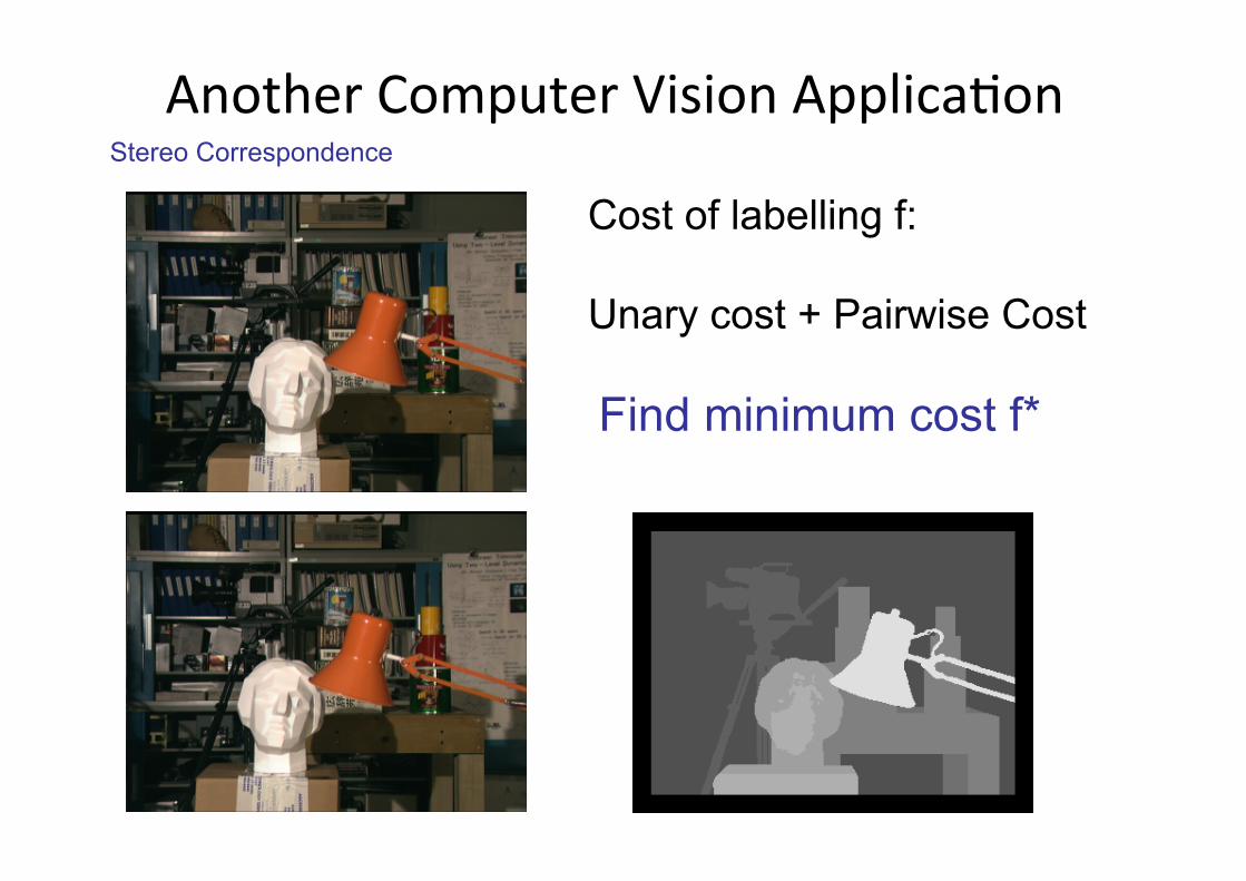
Stereo Correspondence
Cost of labelling f: Unary cost + Pairwise Cost
Find minimum cost f*
AnotherComputerVisionApplicaQon
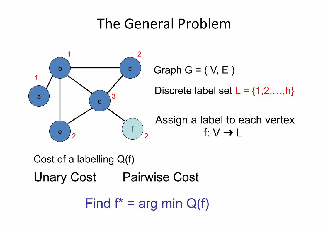
TheGeneralProblem
b
a
e
d
c
f
Graph G = ( V, E )
Discrete label set L = {1,2,…,h}
Assign a label to each vertex f: V ➜ L
1
1 2
2 2
3
Cost of a labelling Q(f)
Unary Cost Pairwise Cost
Find f* = arg min Q(f)
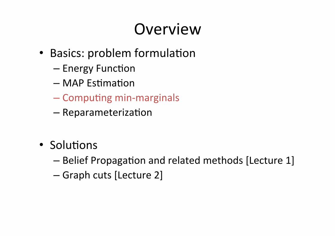
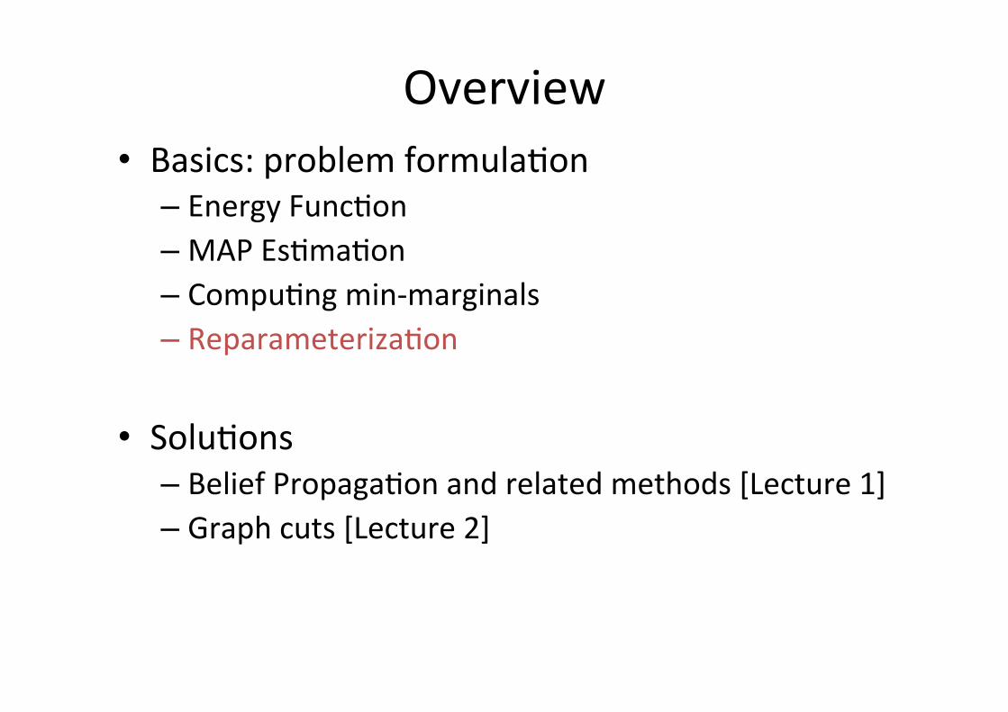
Overview• Basics:problemformulaQon
– EnergyFuncQon– MAPEsQmaQon– CompuQngmin-marginals– ReparameterizaQon
• SoluQons
– BeliefPropagaQonandrelatedmethods[Lecture1]– Graphcuts[Lecture2]

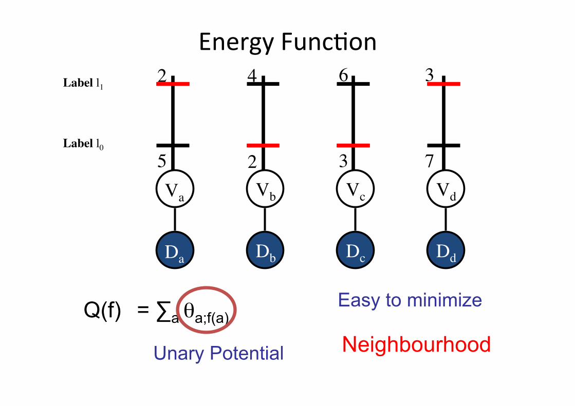
EnergyFuncQon
Va Vb Vc Vd
Label l0
Label l1
Da Db Dc Dd
Random Variables V = {Va, Vb, ….}
Labels L = {l0, l1, ….} Data D
Labelling f: {a, b, …. } ➔ {0,1, …}
EnergyFuncQon
Va Vb Vc Vd
Da Db Dc Dd
Q(f) = ∑a θa;f(a)
Unary Potential
2
5
4
2
6
3
3
7Label l0
Label l1
Easy to minimize
Neighbourhood
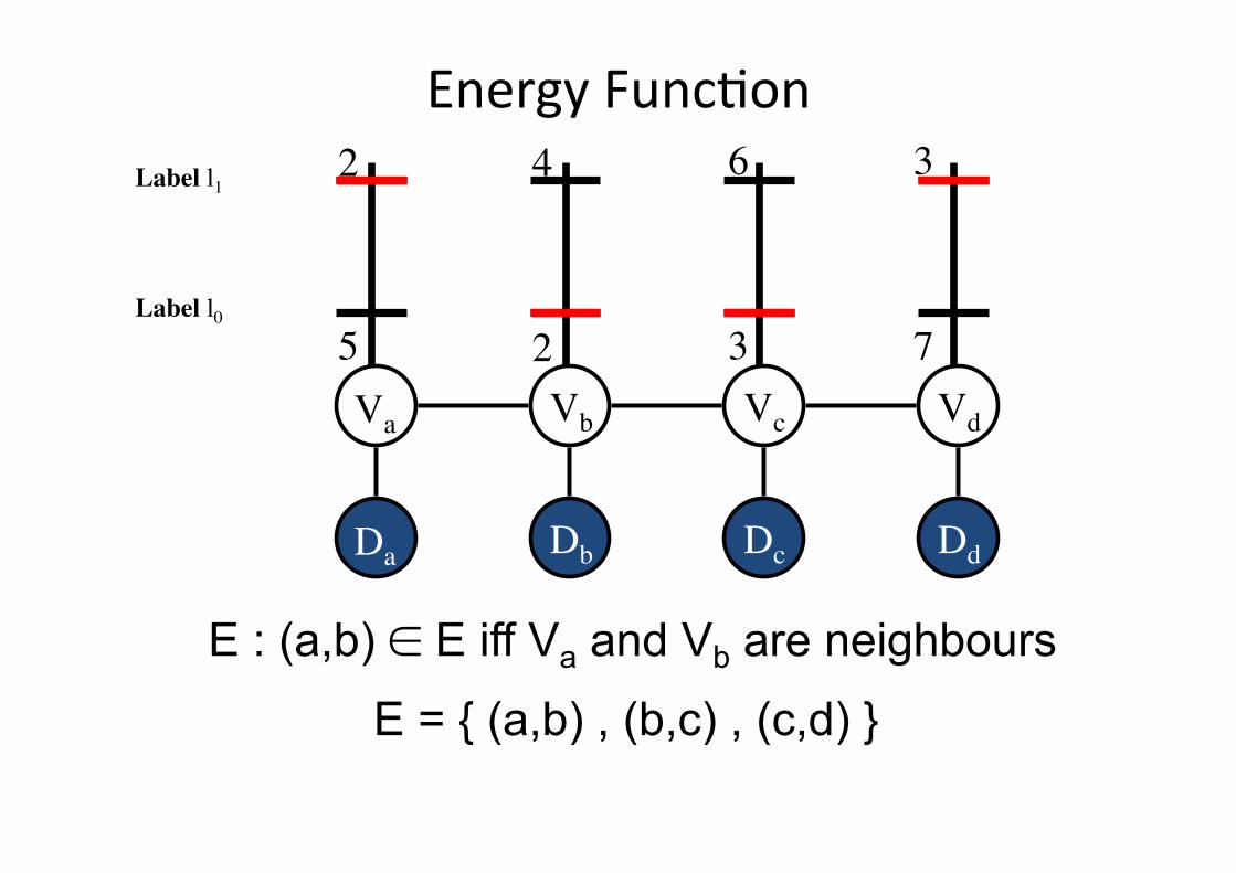
EnergyFuncQon
Va Vb Vc Vd
Da Db Dc Dd
E : (a,b) ∈ E iff Va and Vb are neighbours
E = { (a,b) , (b,c) , (c,d) }
2
5
4
2
6
3
3
7Label l0
Label l1
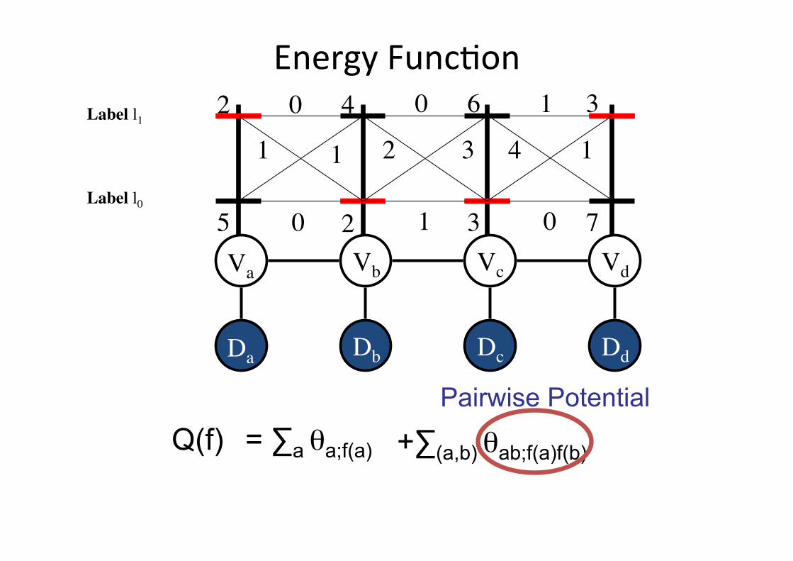
EnergyFuncQon
Va Vb Vc Vd
Da Db Dc Dd
+∑(a,b) θab;f(a)f(b) Pairwise Potential
0
1 1
0
0
2
1
1
4 1
0
3
2
5
4
2
6
3
3
7Label l0
Label l1
Q(f) = ∑a θa;f(a)

EnergyFuncQon
Va Vb Vc Vd
Da Db Dc Dd
0
1 1
0
0
2
1
1
4 1
0
3
Parameter
2
5
4
2
6
3
3
7Label l0
Label l1
+∑(a,b) θab;f(a)f(b) Q(f; θ) = ∑a θa;f(a)

Overview• Basics:problemformulaQon
– EnergyFuncQon– MAPEsQmaQon– CompuQngmin-marginals– ReparameterizaQon
• SoluQons
– BeliefPropagaQonandrelatedmethods[Lecture1]– Graphcuts[Lecture2]

MAPEsQmaQon
Va Vb Vc Vd
2
5
4
2
6
3
3
7
0
1 1
0
0
2
1
1
4 1
0
3
Q(f; θ) = ∑a θa;f(a) + ∑(a,b) θab;f(a)f(b)
2 + 1 + 2 + 1 + 3 + 1 + 3 = 13
Label l0
Label l1

MAPEsQmaQon
Va Vb Vc Vd
2
5
4
2
6
3
3
7
0
1 1
0
0
2
1
1
4 1
0
3
Q(f; θ) = ∑a θa;f(a) + ∑(a,b) θab;f(a)f(b)
5 + 1 + 4 + 0 + 6 + 4 + 7 = 27
Label l0
Label l1

MAPEsQmaQon
Va Vb Vc Vd
2
5
4
2
6
3
3
7
0
1 1
0
0
2
1
1
4 1
0
3
Q(f; θ) = ∑a θa;f(a) + ∑(a,b) θab;f(a)f(b)
f* = arg min Q(f; θ)
q* = min Q(f; θ) = Q(f*; θ)
Label l0
Label l1
Equivalent to maximizing the associated probability
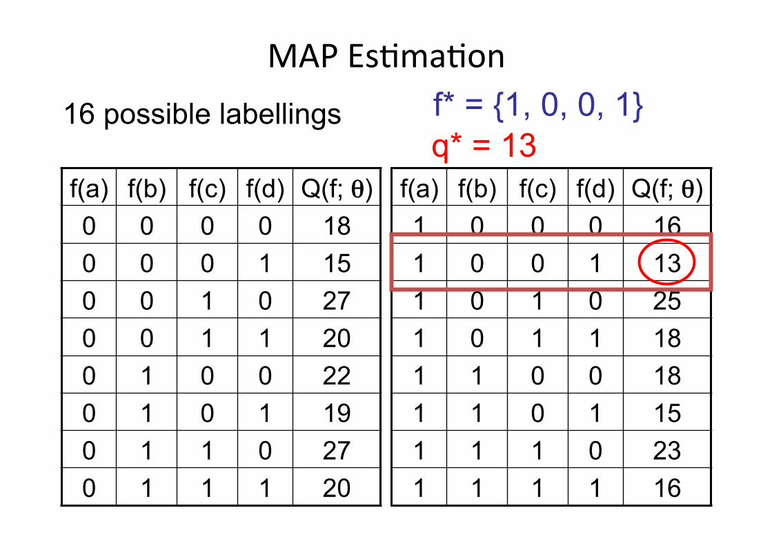
MAPEsQmaQon
f(a) f(b) f(c) f(d) Q(f; θ) 0 0 0 0 18 0 0 0 1 15 0 0 1 0 27 0 0 1 1 20 0 1 0 0 22 0 1 0 1 19 0 1 1 0 27 0 1 1 1 20
16 possible labellings
f(a) f(b) f(c) f(d) Q(f; θ) 1 0 0 0 16 1 0 0 1 13 1 0 1 0 25 1 0 1 1 18 1 1 0 0 18 1 1 0 1 15 1 1 1 0 23 1 1 1 1 16
f* = {1, 0, 0, 1} q* = 13
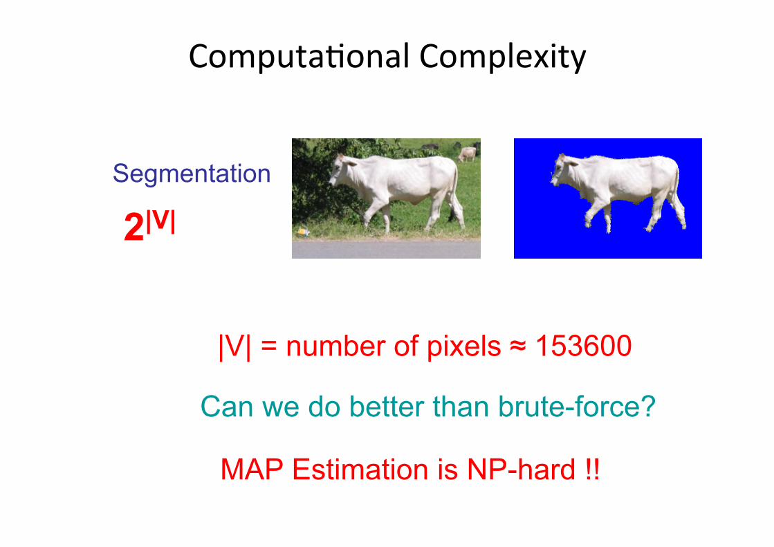
ComputaQonalComplexity
|V| = number of pixels ≈ 153600
Segmentation
2|V|
Can we do better than brute-force?
MAP Estimation is NP-hard !!

MAPInference/EnergyMinimizaQon• CompuQngtheassignmentminimizingtheenergyinNP-hardingeneral
• Exactinferenceispossibleinsomecases,e.g.,– Lowtreewidthgraphsàmessage-passing– SubmodularpotenQalsàgraphcuts
• Efficientapproximateinferencealgorithmsexist– Messagepassingongeneralgraphs– Move-makingalgorithms– RelaxaQonalgorithms
Overview• Basics:problemformulaQon
– EnergyFuncQon– MAPEsQmaQon– CompuQngmin-marginals– ReparameterizaQon
• SoluQons
– BeliefPropagaQonandrelatedmethods[Lecture1]– Graphcuts[Lecture2]
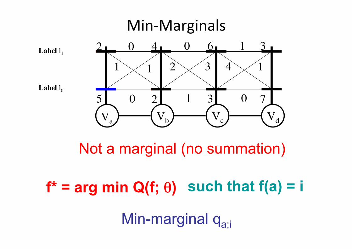
Min-Marginals
Va Vb Vc Vd
2
5
4
2
6
3
3
7
0
1 1
0
0
2
1
1
4 1
0
3
f* = arg min Q(f; θ) such that f(a) = i
Min-marginal qa;i
Label l0
Label l1
Not a marginal (no summation)
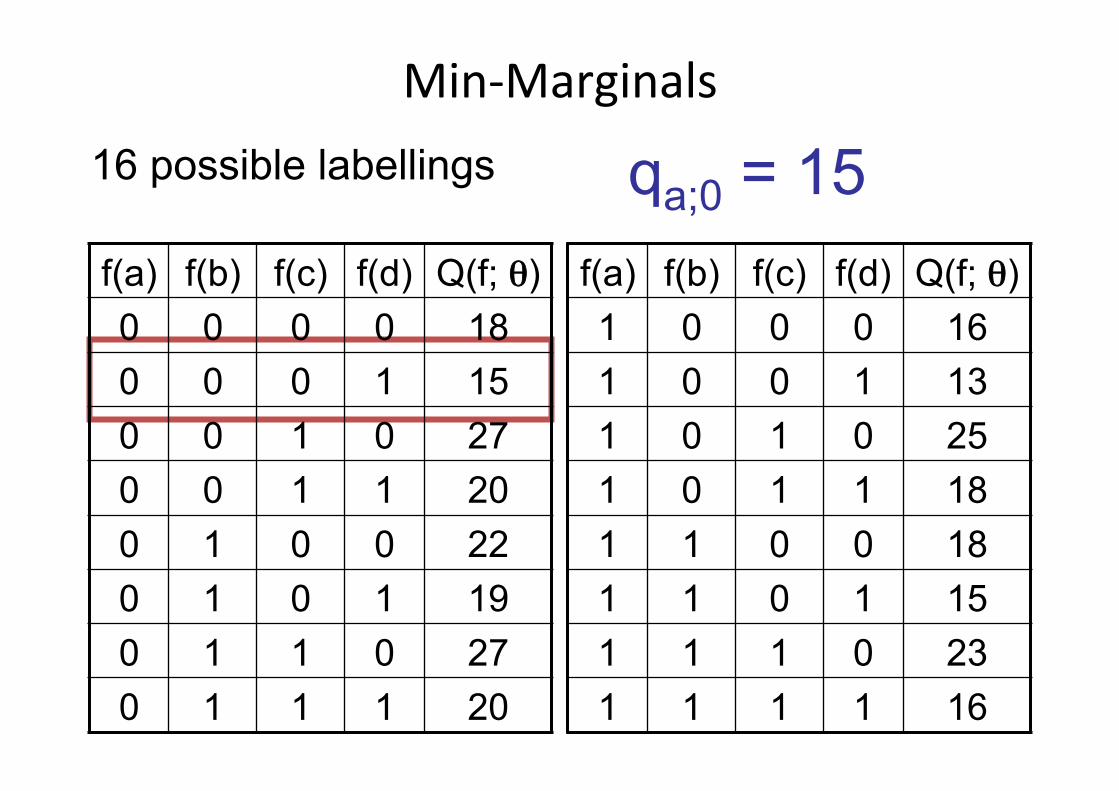
Min-Marginals16 possible labellings qa;0 = 15 f(a) f(b) f(c) f(d) Q(f; θ) 0 0 0 0 18 0 0 0 1 15 0 0 1 0 27 0 0 1 1 20 0 1 0 0 22 0 1 0 1 19 0 1 1 0 27 0 1 1 1 20
f(a) f(b) f(c) f(d) Q(f; θ) 1 0 0 0 16 1 0 0 1 13 1 0 1 0 25 1 0 1 1 18 1 1 0 0 18 1 1 0 1 15 1 1 1 0 23 1 1 1 1 16
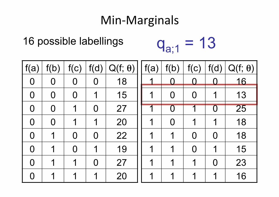
Min-Marginals16 possible labellings qa;1 = 13
f(a) f(b) f(c) f(d) Q(f; θ) 1 0 0 0 16 1 0 0 1 13 1 0 1 0 25 1 0 1 1 18 1 1 0 0 18 1 1 0 1 15 1 1 1 0 23 1 1 1 1 16
f(a) f(b) f(c) f(d) Q(f; θ) 0 0 0 0 18 0 0 0 1 15 0 0 1 0 27 0 0 1 1 20 0 1 0 0 22 0 1 0 1 19 0 1 1 0 27 0 1 1 1 20
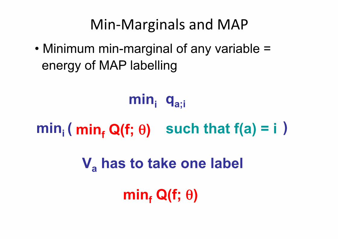
Min-MarginalsandMAP• Minimum min-marginal of any variable = energy of MAP labelling
minf Q(f; θ) such that f(a) = i
qa;i mini
mini ( )
Va has to take one label
minf Q(f; θ)
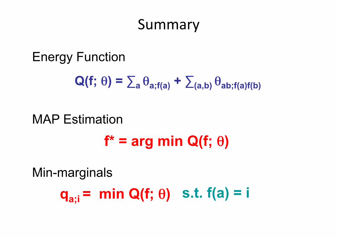
Summary
MAP Estimation
f* = arg min Q(f; θ)
Q(f; θ) = ∑a θa;f(a) + ∑(a,b) θab;f(a)f(b)
Min-marginals
qa;i = min Q(f; θ) s.t. f(a) = i
Energy Function
Overview• Basics:problemformulaQon
– EnergyFuncQon– MAPEsQmaQon– CompuQngmin-marginals– ReparameterizaQon
• SoluQons
– BeliefPropagaQonandrelatedmethods[Lecture1]– Graphcuts[Lecture2]
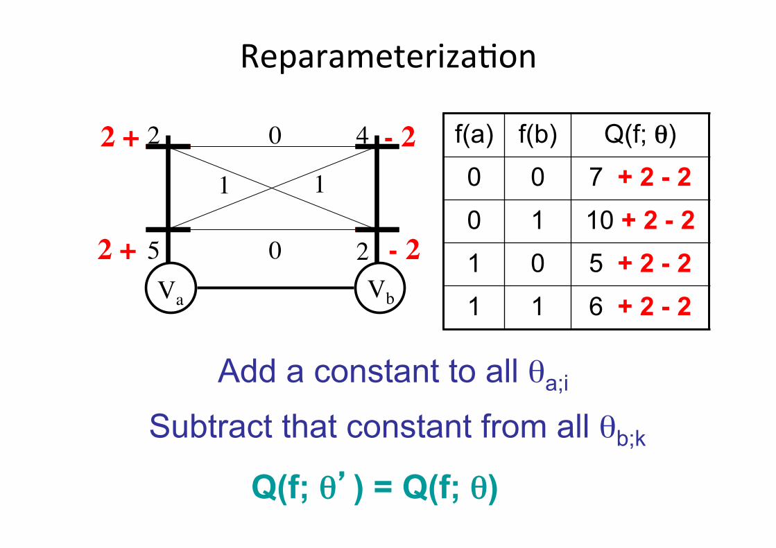
ReparameterizaQon
f(a) f(b) Q(f; θ)
0 0 7 + 2 - 2
0 1 10 + 2 - 2
1 0 5 + 2 - 2
1 1 6 + 2 - 2
Add a constant to all θa;i
Subtract that constant from all θb;k
Q(f; θ’) = Q(f; θ)
Va Vb
2
5
4
2
0
0
2 +
2 +
- 2
- 2
1 1

ReparameterizaQon
Va Vb
2
5
4
2
0
1 1
0
f(a) f(b) Q(f; θ)
0 0 7
0 1 10 - 3 + 3
1 0 5
1 1 6 - 3 + 3
- 3 + 3- 3
Q(f; θ’) = Q(f; θ)
Add a constant to one θb;k
Subtract that constant from θab;ik for all ‘i’

ReparameterizaQon
Q(f; θ’) = Q(f; θ), for all f
θ’ is a reparameterization of θ, iff
θ’ ≡ θ
θ’b;k = θb;k
θ’a;i = θa;i
θ’ab;ik = θab;ik
+ Mab;k
- Mab;k
+ Mba;i
- Mba;i
Equivalently Kolmogorov, PAMI, 2006
Va Vb
2
5
4
2
0
0
2 +
2 +
- 2
- 2
1 1
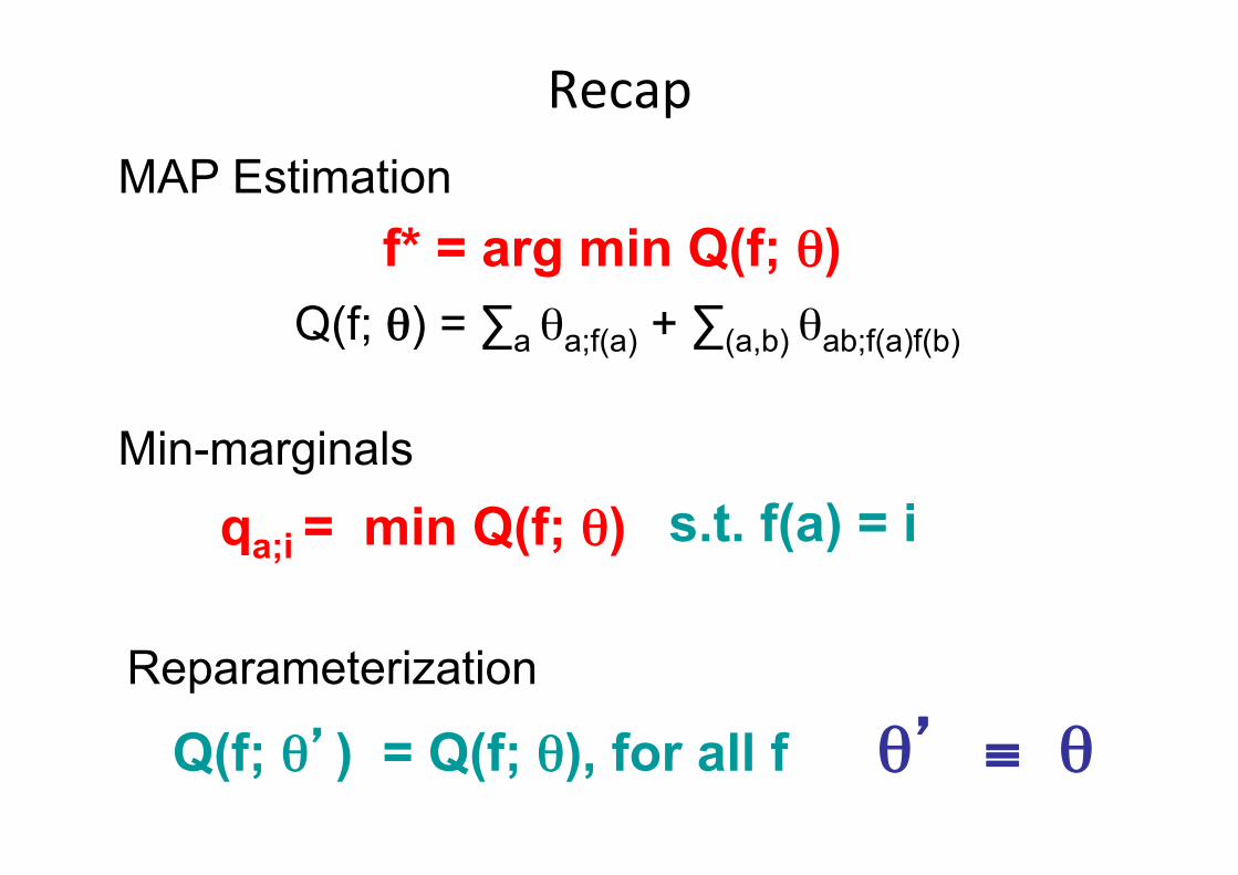
RecapMAP Estimation
f* = arg min Q(f; θ) Q(f; θ) = ∑a θa;f(a) + ∑(a,b) θab;f(a)f(b)
Min-marginals
qa;i = min Q(f; θ) s.t. f(a) = i
Q(f; θ’) = Q(f; θ), for all f θ’ ≡ θ Reparameterization

Overview• Basics:problemformulaQon
– EnergyFuncQon– MAPEsQmaQon– CompuQngmin-marginals– ReparameterizaQon
• SoluQons
– BeliefPropagaQonandrelatedmethods[Lecture1]– Graphcuts[Lecture2]
BeliefPropagaQon
• Belief Propagation gives exact MAP for chains
• Remember, some MAP problems are easy
• Exact MAP for trees
• Clever Reparameterization
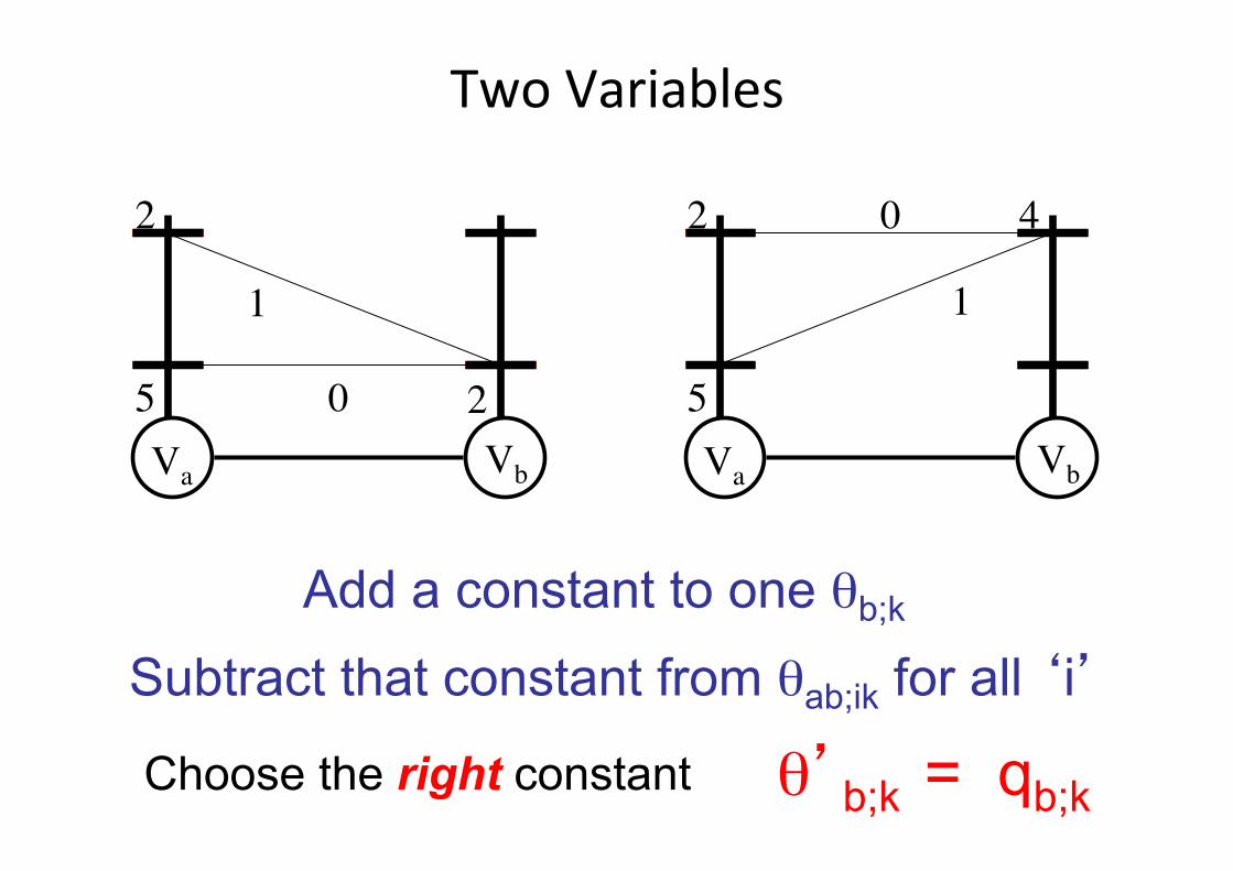
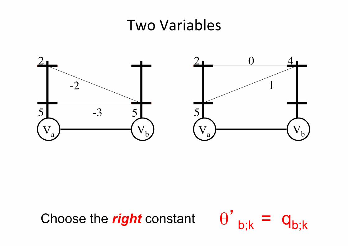
TwoVariables
Va Vb
2
5 2
1
0Va Vb
2
5
40
1
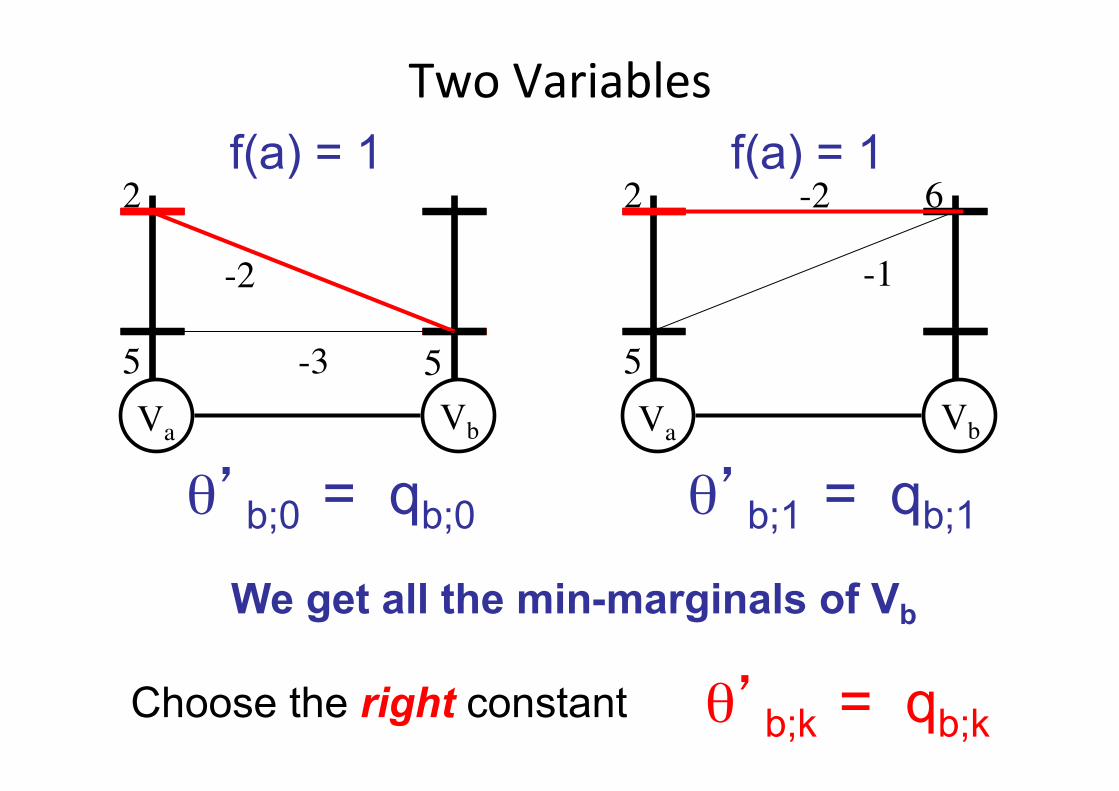
Choose the right constant θ’b;k = qb;k
Add a constant to one θb;k
Subtract that constant from θab;ik for all ‘i’
Va Vb
2
5 2
1
0Va Vb
2
5
40
1
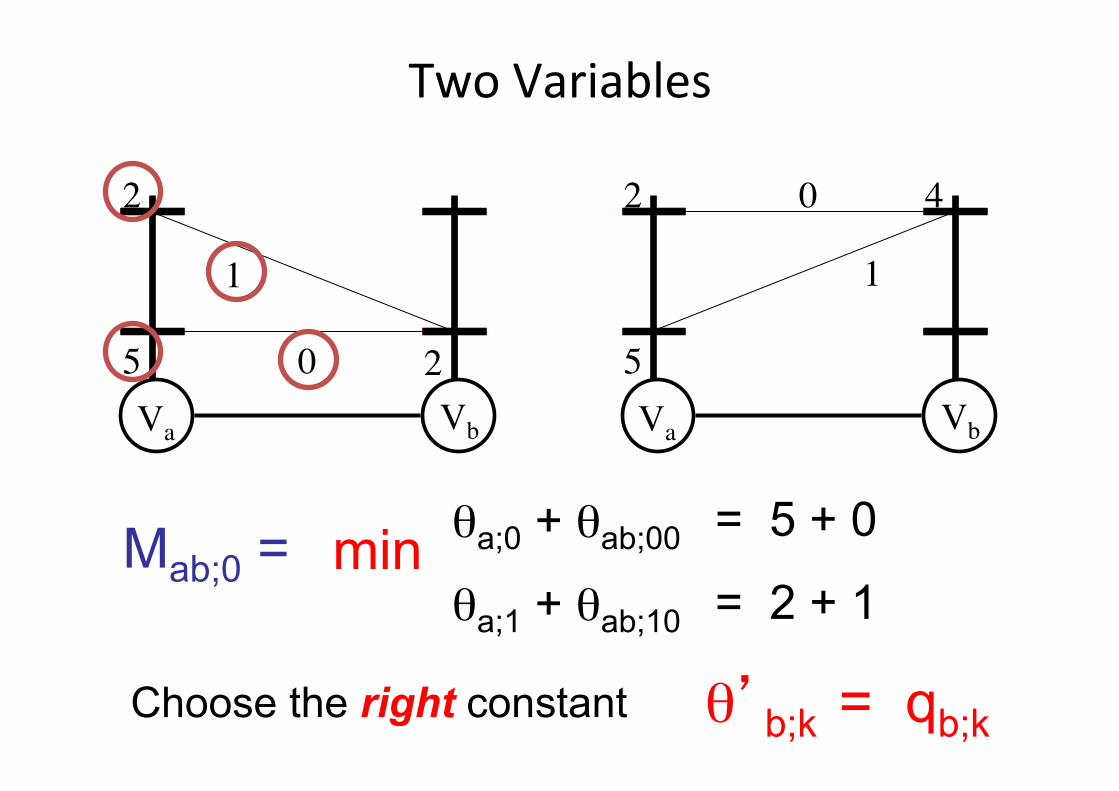
Choose the right constant θ’b;k = qb;k
θa;0 + θab;00 = 5 + 0
θa;1 + θab;10 = 2 + 1 min Mab;0 =
TwoVariables
Va Vb
2
5 5
-2
-3Va Vb
2
5
40
1
Choose the right constant θ’b;k = qb;k
TwoVariables

Va Vb
2
5 5
-2
-3Va Vb
2
5
40
1
Choose the right constant θ’b;k = qb;k
f(a) = 1
θ’b;0 = qb;0
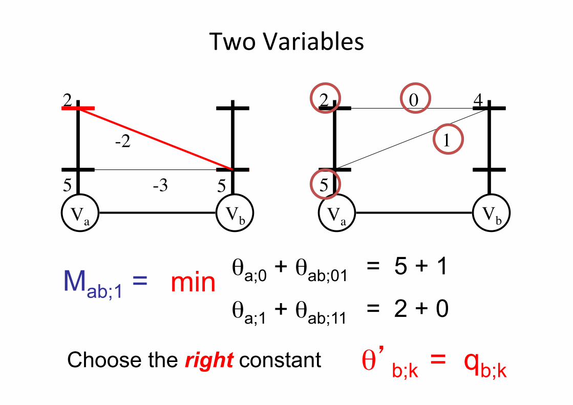
TwoVariables
Potentials along the red path add up to 0
Va Vb
2
5 5
-2
-3Va Vb
2
5
40
1
Choose the right constant θ’b;k = qb;k
θa;0 + θab;01 = 5 + 1
θa;1 + θab;11 = 2 + 0 min Mab;1 =
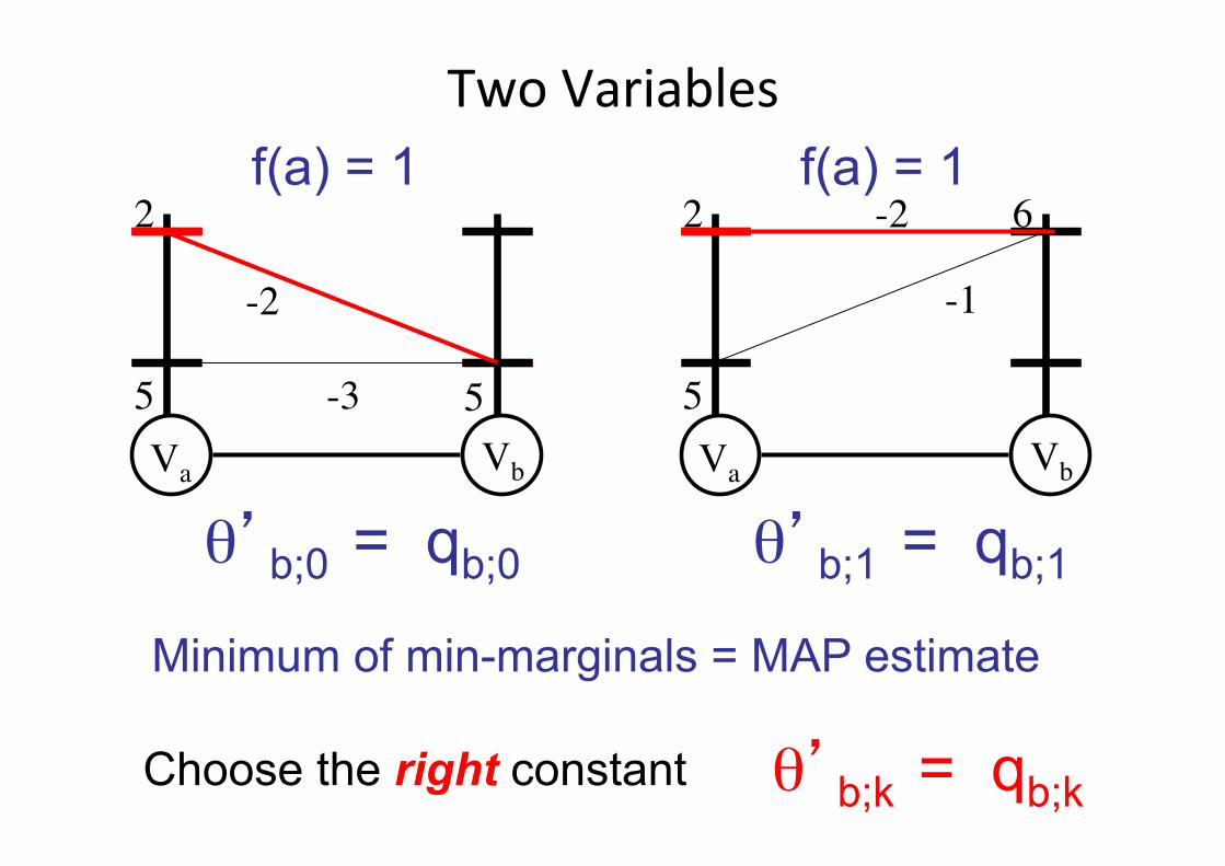
TwoVariables
Va Vb
2
5 5
-2
-3Va Vb
2
5
6-2
-1
Choose the right constant θ’b;k = qb;k
f(a) = 1
θ’b;0 = qb;0
f(a) = 1
θ’b;1 = qb;1
Minimum of min-marginals = MAP estimate
TwoVariables
Va Vb
2
5 5
-2
-3Va Vb
2
5
6-2
-1
Choose the right constant θ’b;k = qb;k
f(a) = 1
θ’b;0 = qb;0
f(a) = 1
θ’b;1 = qb;1
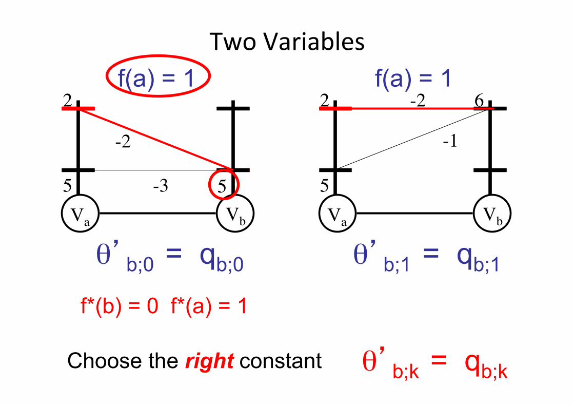
f*(b) = 0 f*(a) = 1
TwoVariables
Va Vb
2
5 5
-2
-3Va Vb
2
5
6-2
-1
Choose the right constant θ’b;k = qb;k
f(a) = 1
θ’b;0 = qb;0
f(a) = 1
θ’b;1 = qb;1
We get all the min-marginals of Vb
TwoVariables
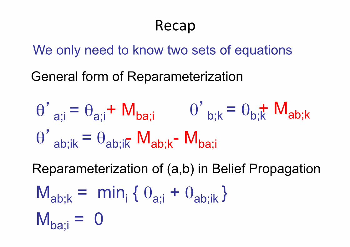
RecapWe only need to know two sets of equations
General form of Reparameterization
θ’a;i = θa;i
θ’ab;ik = θab;ik
+ Mab;k
- Mab;k
+ Mba;i
- Mba;i
θ’b;k = θb;k
Reparameterization of (a,b) in Belief Propagation
Mab;k = mini { θa;i + θab;ik } Mba;i = 0

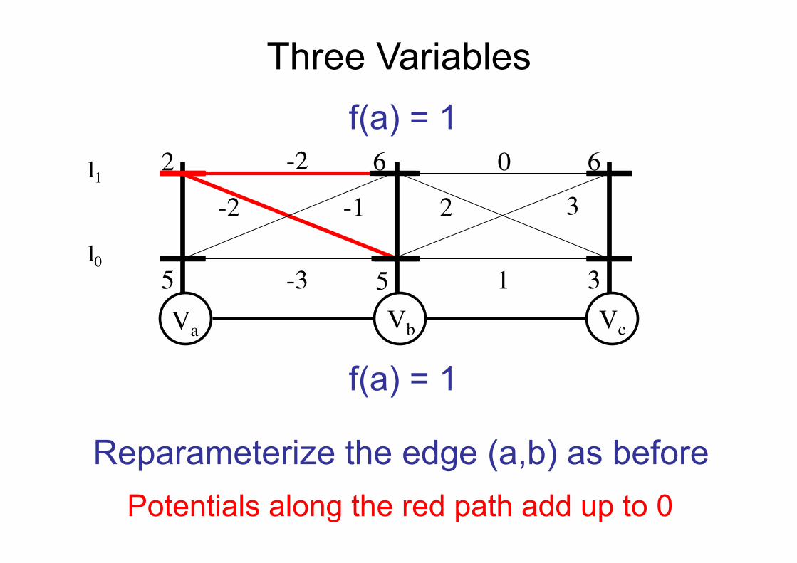
Three Variables
Va Vb
2
5 2
1
0Vc
4 60
1
0
1
3
2 3
Reparameterize the edge (a,b) as before
l0
l1
Va Vb
2
5 5-3Vc
6 60
1
-2
3
Reparameterize the edge (a,b) as before
f(a) = 1
f(a) = 1
Potentials along the red path add up to 0
-2 -1 2 3
Three Variables
l0
l1
Va Vb
2
5 5-3Vc
6 12-6
-5
-2
9
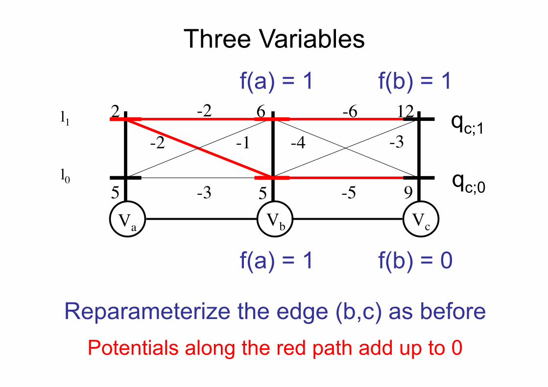
Reparameterize the edge (b,c) as before
f(a) = 1
f(a) = 1
Potentials along the red path add up to 0
f(b) = 1
f(b) = 0
qc;0
qc;1 -2 -1 -4 -3
Three Variables
l0
l1
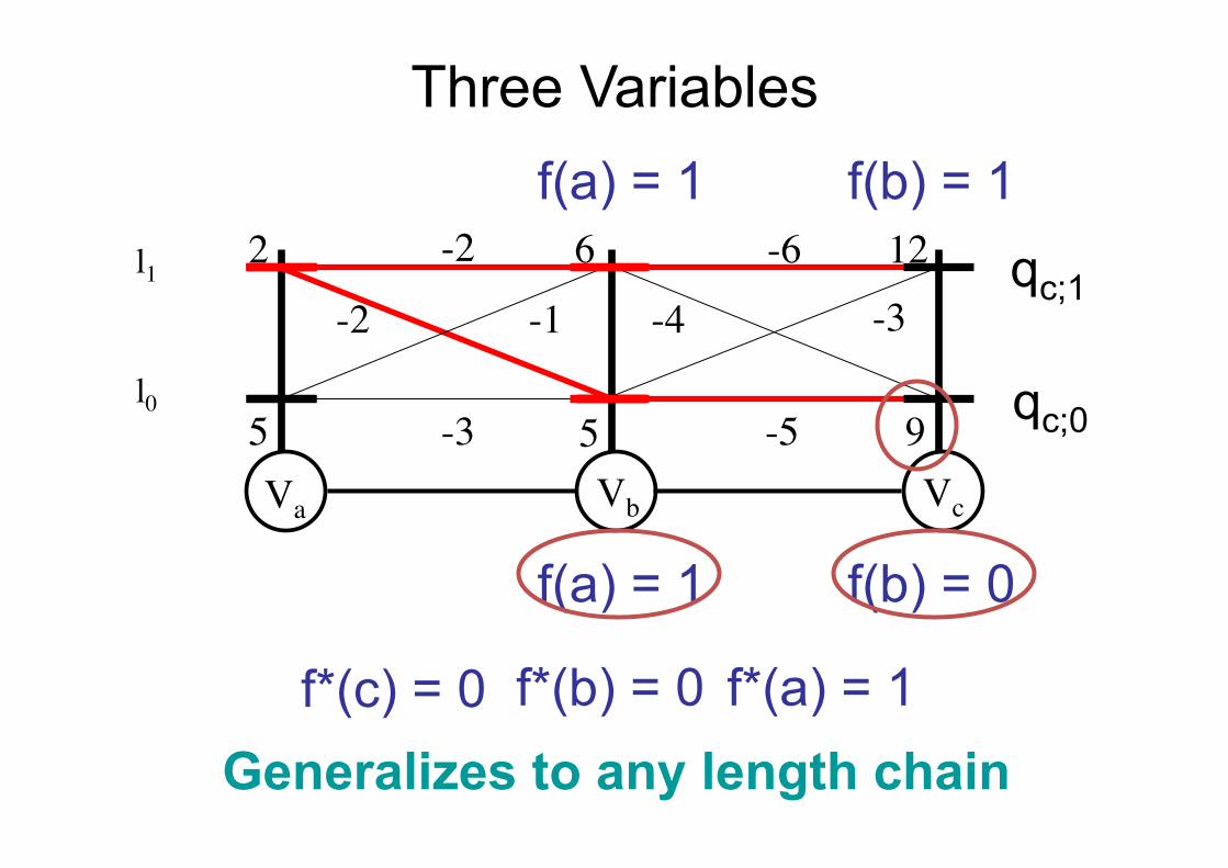
Va Vb
2
5 5-3Vc
6 12-6
-5
-2
9
f(a) = 1
f(a) = 1
f(b) = 1
f(b) = 0
qc;0
qc;1
f*(c) = 0 f*(b) = 0 f*(a) = 1 Generalizes to any length chain
-2 -1 -4 -3
Three Variables
l0
l1

Va Vb
2
5 5-3Vc
6 12-6
-5
-2
9
f(a) = 1
f(a) = 1
f(b) = 1
f(b) = 0
qc;0
qc;1
f*(c) = 0 f*(b) = 0 f*(a) = 1 Only Dynamic Programming
-2 -1 -4 -3
Three Variables
l0
l1
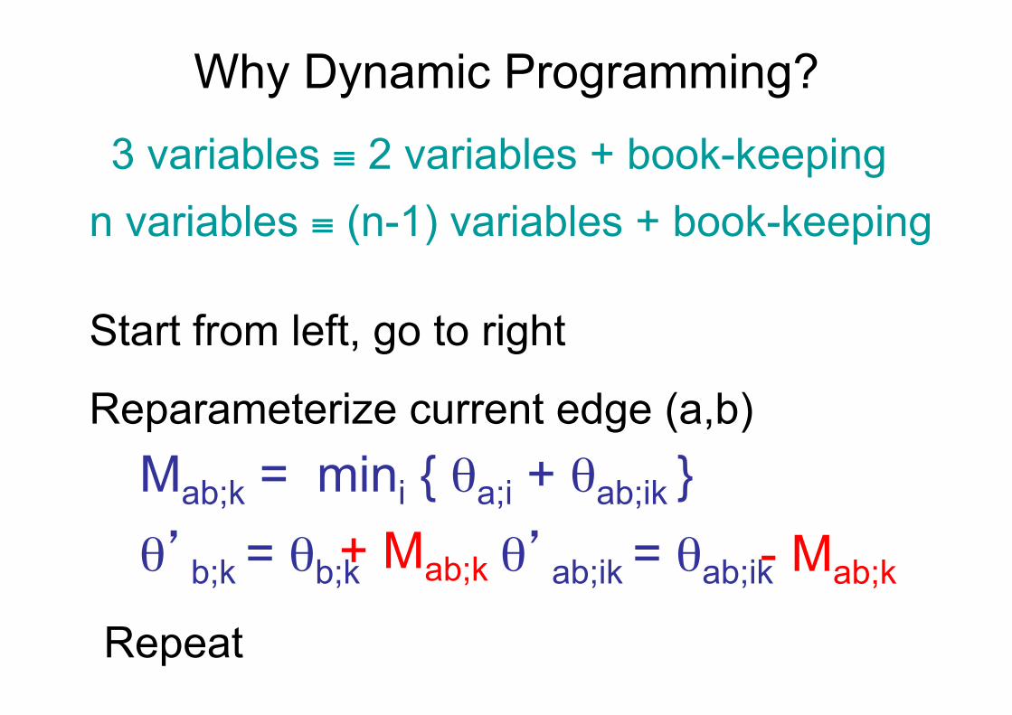
Why Dynamic Programming?
3 variables ≡ 2 variables + book-keeping n variables ≡ (n-1) variables + book-keeping
Start from left, go to right
Reparameterize current edge (a,b) Mab;k = mini { θa;i + θab;ik }
θ’ab;ik = θab;ik + Mab;k - Mab;k θ’b;k = θb;k
Repeat
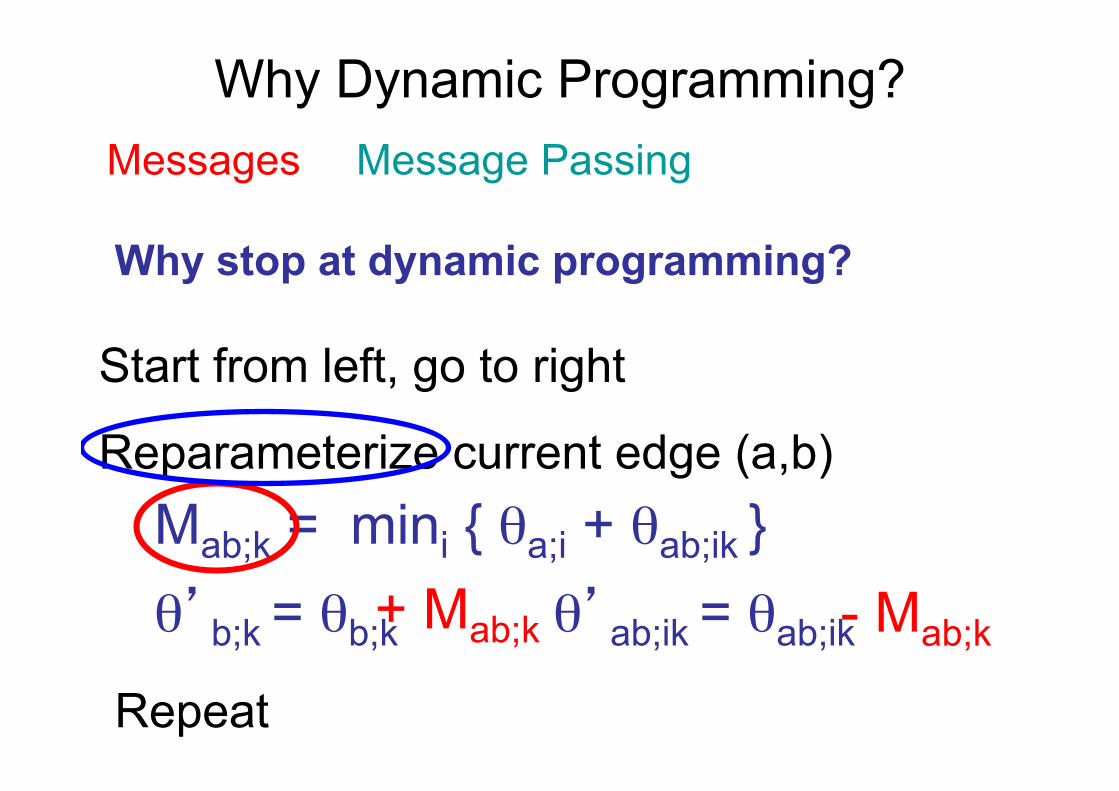
Why Dynamic Programming?
Start from left, go to right
Reparameterize current edge (a,b) Mab;k = mini { θa;i + θab;ik }
θ’ab;ik = θab;ik + Mab;k - Mab;k θ’b;k = θb;k
Repeat
Messages Message Passing
Why stop at dynamic programming?
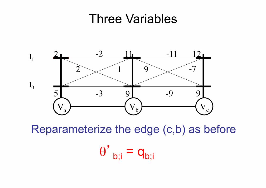
Va Vb
2
5 9-3Vc
11 12-11
-9
-2
9
Reparameterize the edge (c,b) as before
-2 -1 -9 -7
θ’b;i = qb;i
Three Variables
l0
l1
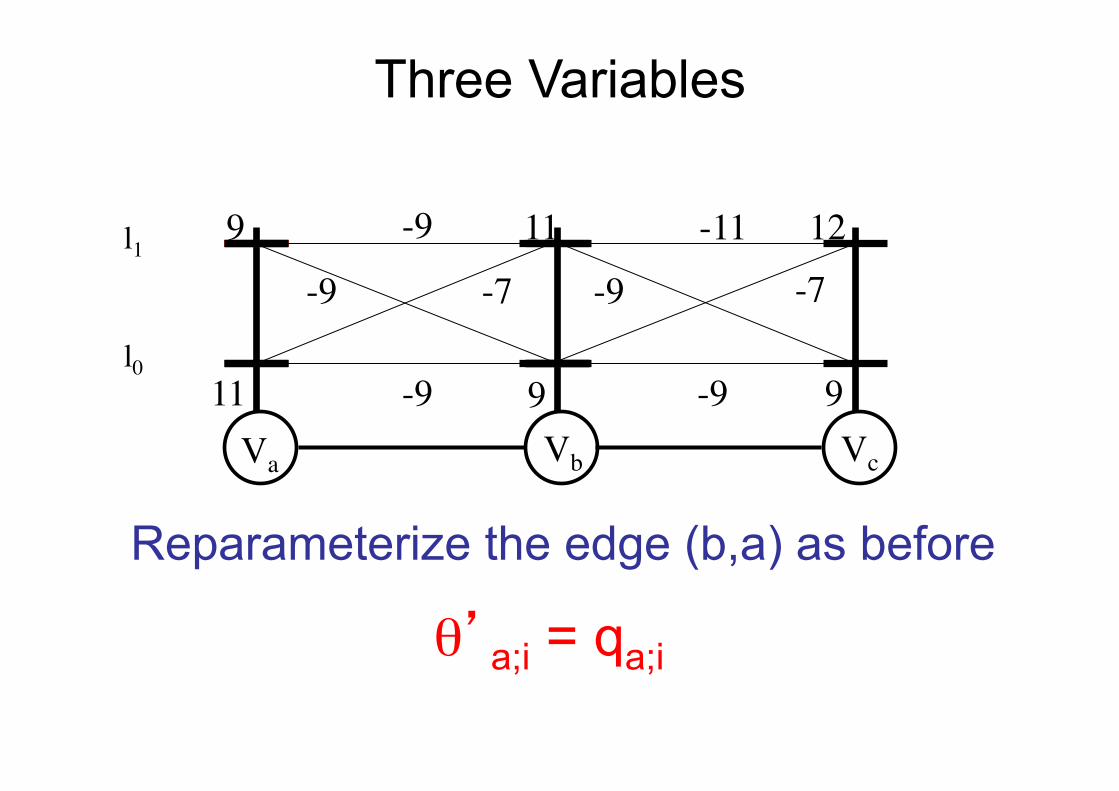
Va Vb
9
11 9-9Vc
11 12-11
-9
-9
9
Reparameterize the edge (b,a) as before
-9 -7 -9 -7
θ’a;i = qa;i
Three Variables
l0
l1
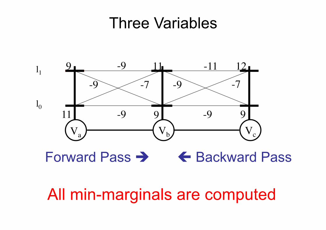
Va Vb
9
11 9-9Vc
11 12-11
-9
-9
9
Forward Pass è ç Backward Pass
-9 -7 -9 -7
All min-marginals are computed
Three Variables
l0
l1
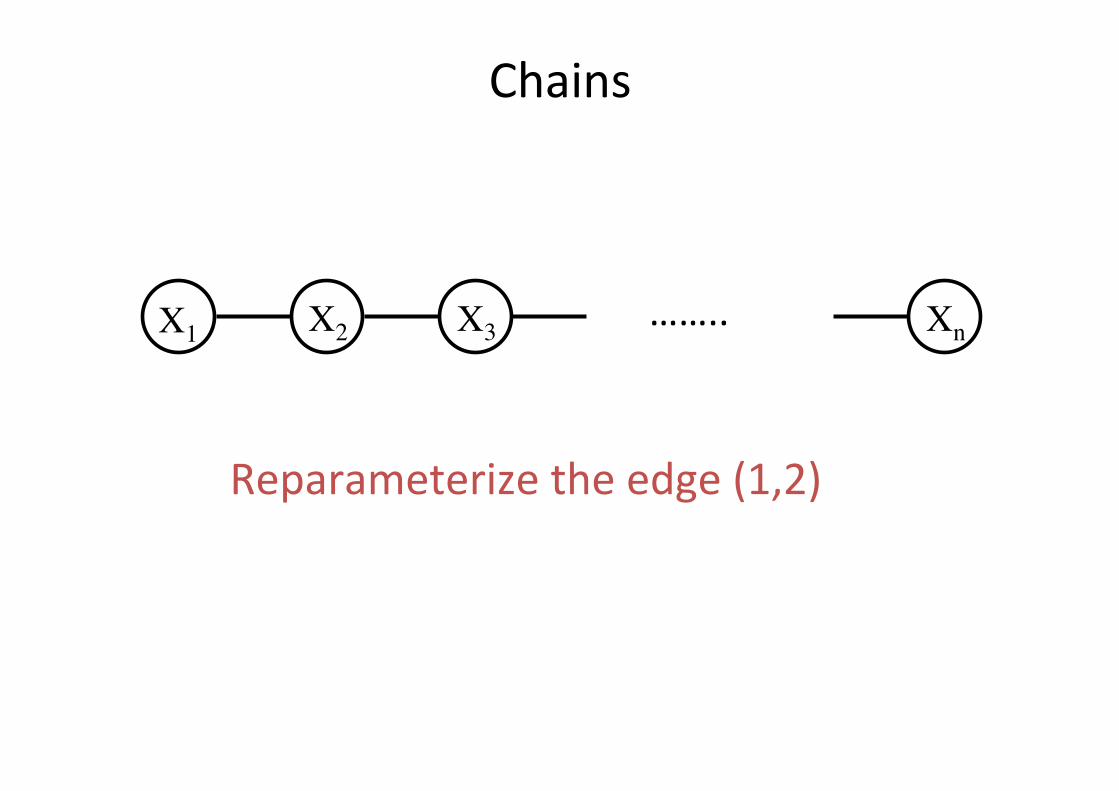
Chains
X1 X2 X3 Xn……..
Reparameterizetheedge(1,2)
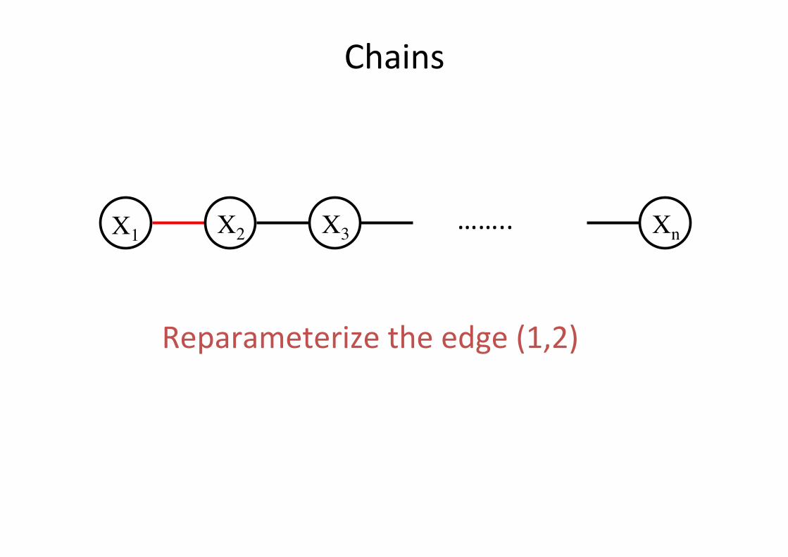
Chains
X1 X2 X3 Xn……..
Reparameterizetheedge(1,2)
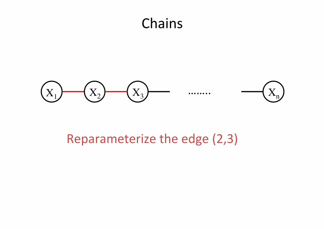
Chains
X1 X2 X3 Xn……..
Reparameterizetheedge(2,3)
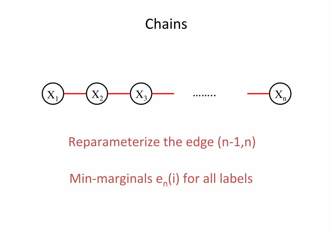
Chains
X1 X2 X3 Xn……..
Reparameterizetheedge(n-1,n)
Min-marginalsen(i)foralllabels
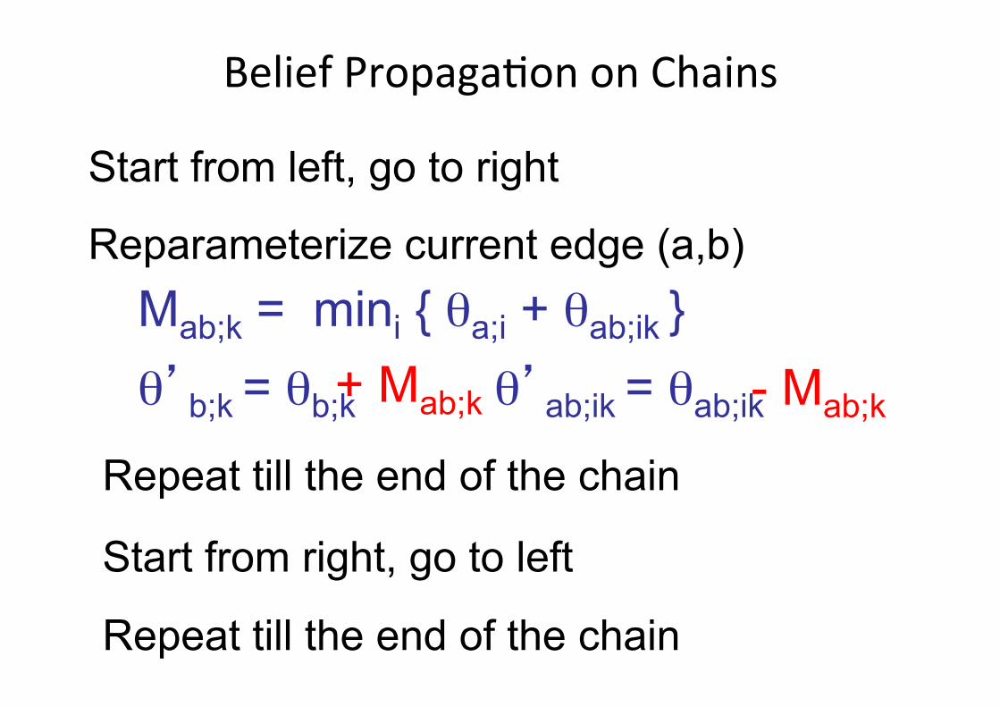
BeliefPropagaQononChains
Start from left, go to right
Reparameterize current edge (a,b) Mab;k = mini { θa;i + θab;ik }
θ’ab;ik = θab;ik + Mab;k - Mab;k θ’b;k = θb;k
Repeat till the end of the chain
Start from right, go to left
Repeat till the end of the chain

BeliefPropagaQononChains
• A way of computing reparam constants
• Generalizes to chains of any length
• Forward Pass - Start to End • MAP estimate • Min-marginals of final variable
• Backward Pass - End to start • All other min-marginals
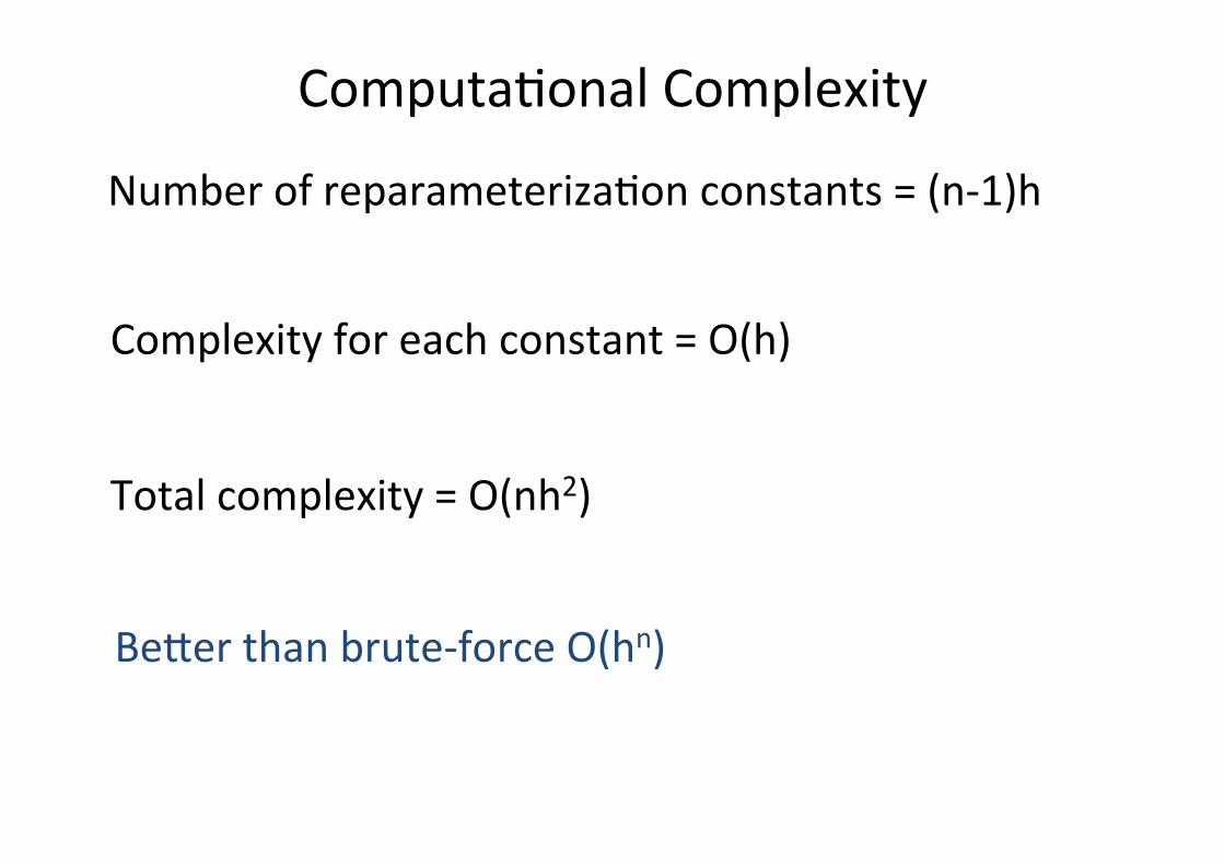
ComputaQonalComplexity
NumberofreparameterizaQonconstants=(n-1)h
Complexityforeachconstant=O(h)
Totalcomplexity=O(nh2)
Be;erthanbrute-forceO(hn)

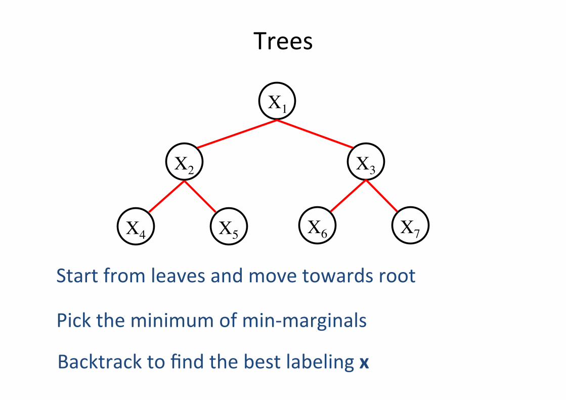
Trees
X2
X1
X3
X4 X5 X6 X7
Reparameterizetheedge(4,2)

Trees
X2
X1
X3
X4 X5 X6 X7
Reparameterizetheedge(3,1)
Min-marginalse1(i)foralllabels
Trees
X2
X1
X3
X4 X5 X6 X7
Startfromleavesandmovetowardsroot
Picktheminimumofmin-marginals
Backtracktofindthebestlabelingx

ComputaQonalComplexity
NumberofreparameterizaQonconstants=(n-1)h
Complexityforeachconstant=O(h)
Totalcomplexity=O(nh2)
Be;erthanbrute-forceO(hn)
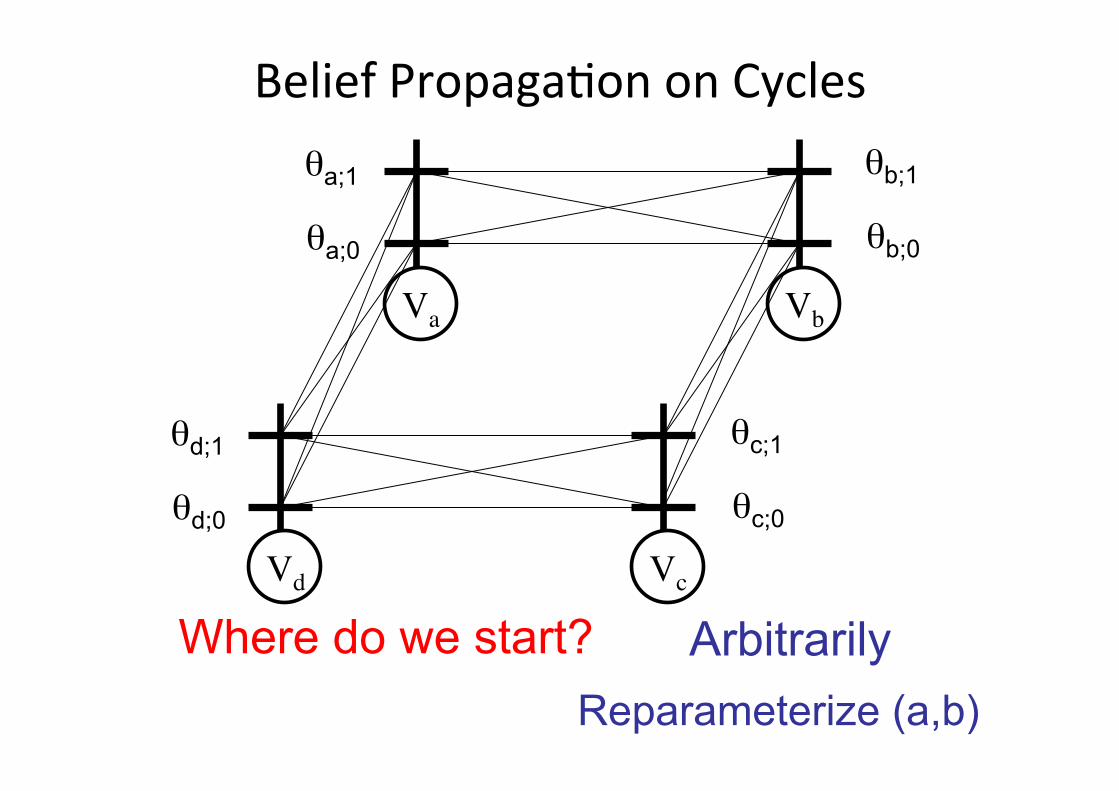
BeliefPropagaQononCycles
Va Vb
Vd Vc
Where do we start? Arbitrarily
θa;0
θa;1
θb;0
θb;1
θd;0
θd;1
θc;0
θc;1
Reparameterize (a,b)

BeliefPropagaQononCycles
Va Vb
Vd Vc
θa;0
θa;1
θ’b;0
θ’b;1
θd;0
θd;1
θc;0
θc;1
Potentials along the red path add up to 0

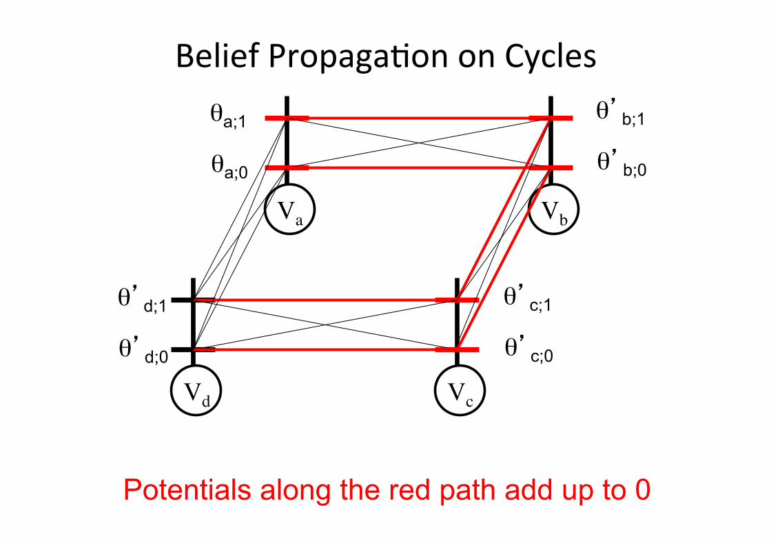
BeliefPropagaQononCycles
Va Vb
Vd Vc
θa;0
θa;1
θ’b;0
θ’b;1
θd;0
θd;1
θ’c;0
θ’c;1
Potentials along the red path add up to 0
BeliefPropagaQononCycles
Va Vb
Vd Vc
θa;0
θa;1
θ’b;0
θ’b;1
θ’d;0
θ’d;1
θ’c;0
θ’c;1
Potentials along the red path add up to 0
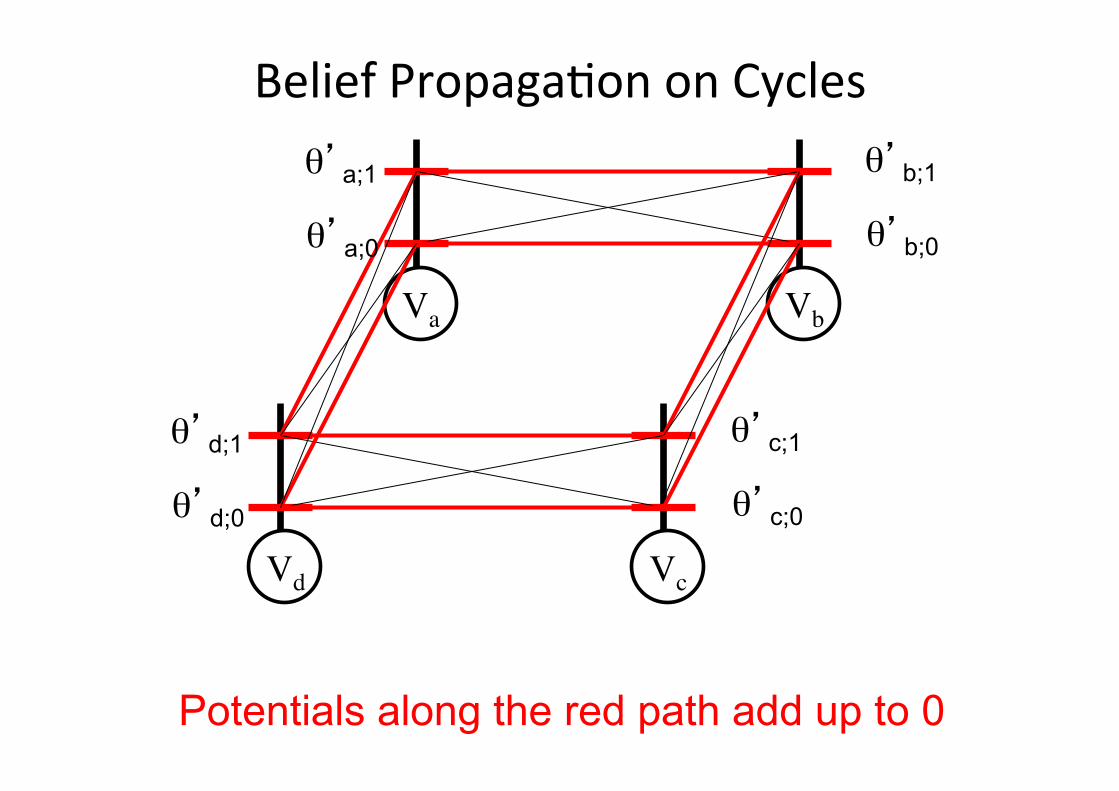
BeliefPropagaQononCycles
Va Vb
Vd Vc
θ’a;0
θ’a;1
θ’b;0
θ’b;1
θ’d;0
θ’d;1
θ’c;0
θ’c;1
Potentials along the red path add up to 0
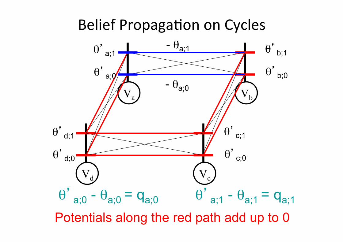
BeliefPropagaQononCycles
Va Vb
Vd Vc
θ’a;0
θ’a;1
θ’b;0
θ’b;1
θ’d;0
θ’d;1
θ’c;0
θ’c;1
Potentials along the red path add up to 0
- θa;0
- θa;1
θ’a;0 - θa;0 = qa;0 θ’a;1 - θa;1 = qa;1
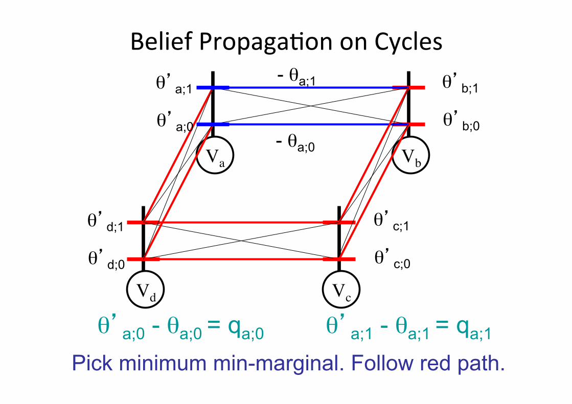
BeliefPropagaQononCycles
Va Vb
Vd Vc
θ’a;0
θ’a;1
θ’b;0
θ’b;1
θ’d;0
θ’d;1
θ’c;0
θ’c;1
Pick minimum min-marginal. Follow red path.
- θa;0
- θa;1
θ’a;0 - θa;0 = qa;0 θ’a;1 - θa;1 = qa;1
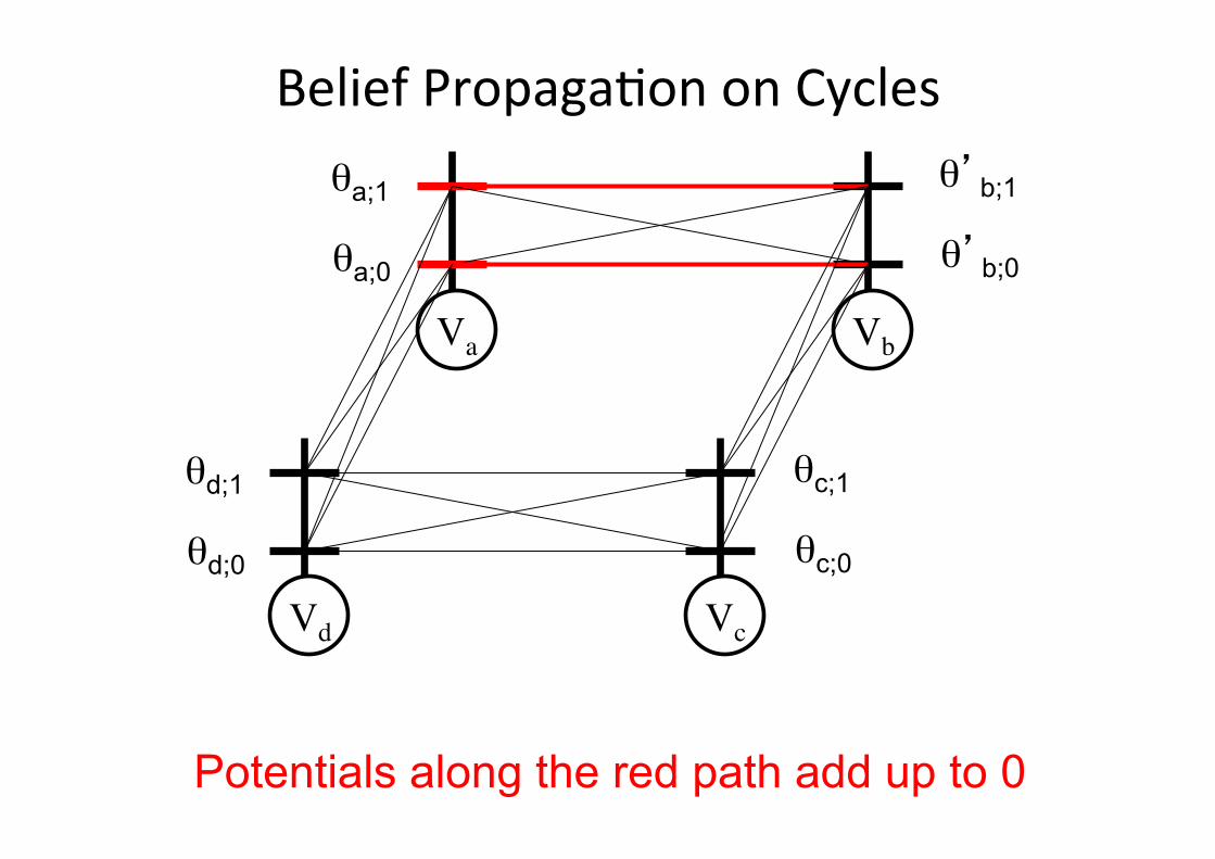
BeliefPropagaQononCycles
Va Vb
Vd Vc
θa;0
θa;1
θ’b;0
θ’b;1
θd;0
θd;1
θc;0
θc;1
Potentials along the red path add up to 0

BeliefPropagaQononCycles
Va Vb
Vd Vc
θa;0
θa;1
θ’b;0
θ’b;1
θd;0
θd;1
θ’c;0
θ’c;1
Potentials along the red path add up to 0
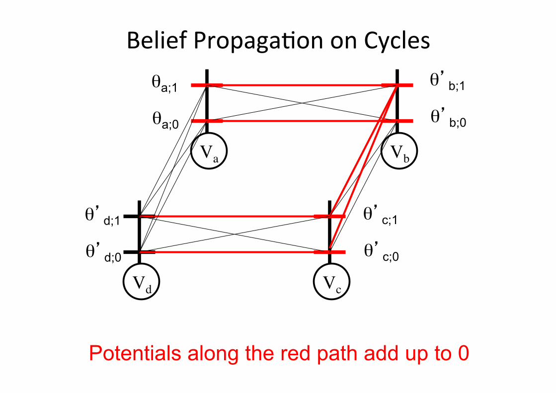
BeliefPropagaQononCycles
Va Vb
Vd Vc
θa;0
θa;1
θ’b;0
θ’b;1
θ’d;0
θ’d;1
θ’c;0
θ’c;1
Potentials along the red path add up to 0

BeliefPropagaQononCycles
Va Vb
Vd Vc
θ’a;0
θ’a;1
θ’b;0
θ’b;1
θ’d;0
θ’d;1
θ’c;0
θ’c;1
Potentials along the red path add up to 0
- θa;0
- θa;1
θ’a;1 - θa;1 = qa;1 θ’a;0 - θa;0 = qa;0 ≤
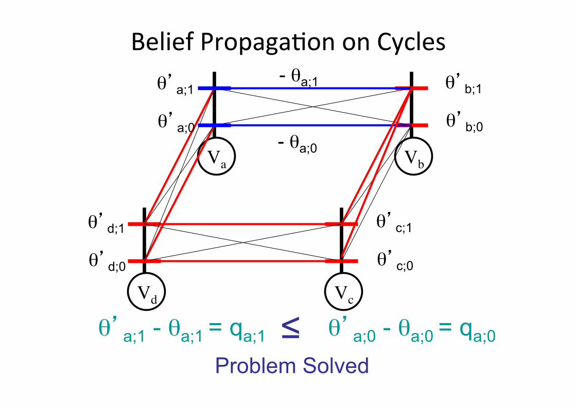
BeliefPropagaQononCycles
Va Vb
Vd Vc
θ’a;0
θ’a;1
θ’b;0
θ’b;1
θ’d;0
θ’d;1
θ’c;0
θ’c;1
Problem Solved
- θa;0
- θa;1
θ’a;1 - θa;1 = qa;1 θ’a;0 - θa;0 = qa;0 ≤
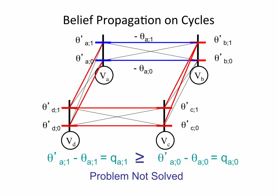
BeliefPropagaQononCycles
Va Vb
Vd Vc
θ’a;0
θ’a;1
θ’b;0
θ’b;1
θ’d;0
θ’d;1
θ’c;0
θ’c;1
Problem Not Solved
- θa;0
- θa;1
θ’a;1 - θa;1 = qa;1 θ’a;0 - θa;0 = qa;0 ≥
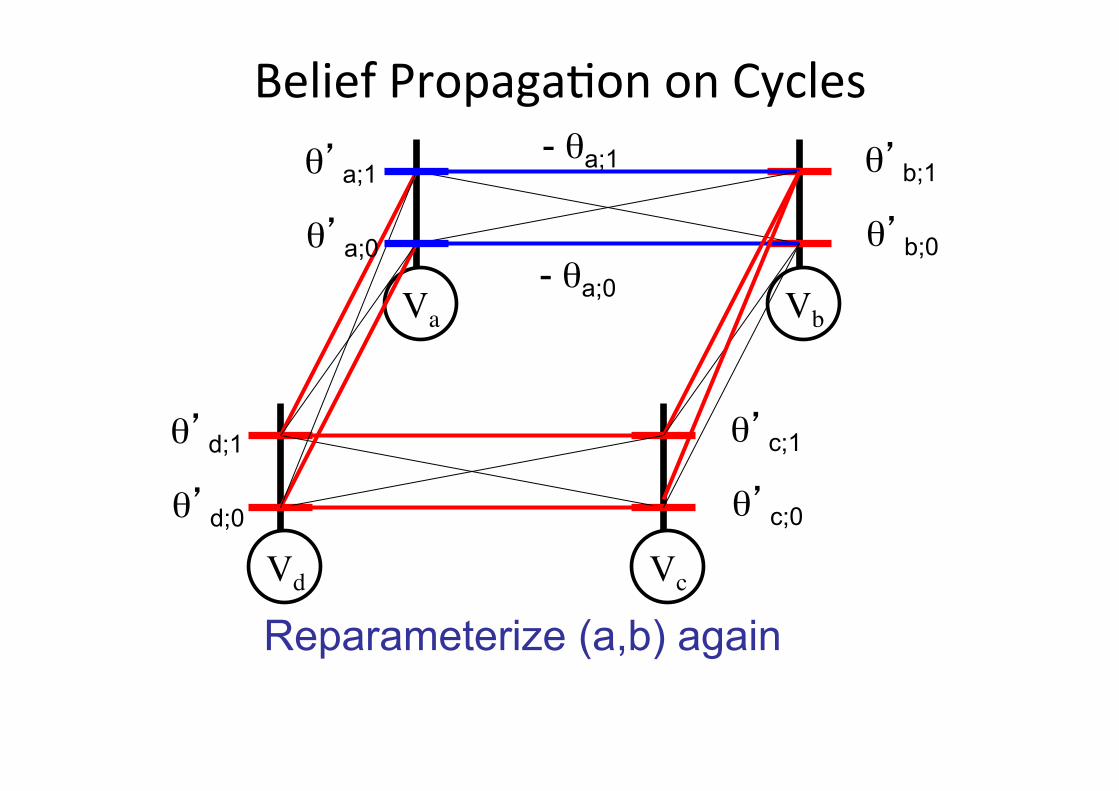
BeliefPropagaQononCycles
Va Vb
Vd Vc
θ’a;0
θ’a;1
θ’b;0
θ’b;1
θ’d;0
θ’d;1
θ’c;0
θ’c;1
- θa;0
- θa;1
Reparameterize (a,b) again

BeliefPropagaQononCycles
Va Vb
Vd Vc
θ’a;0
θ’a;1
θ’’b;0
θ’’b;1
θ’d;0
θ’d;1
θ’c;0
θ’c;1
Reparameterize (a,b) again
But doesn’t this overcount some potentials?
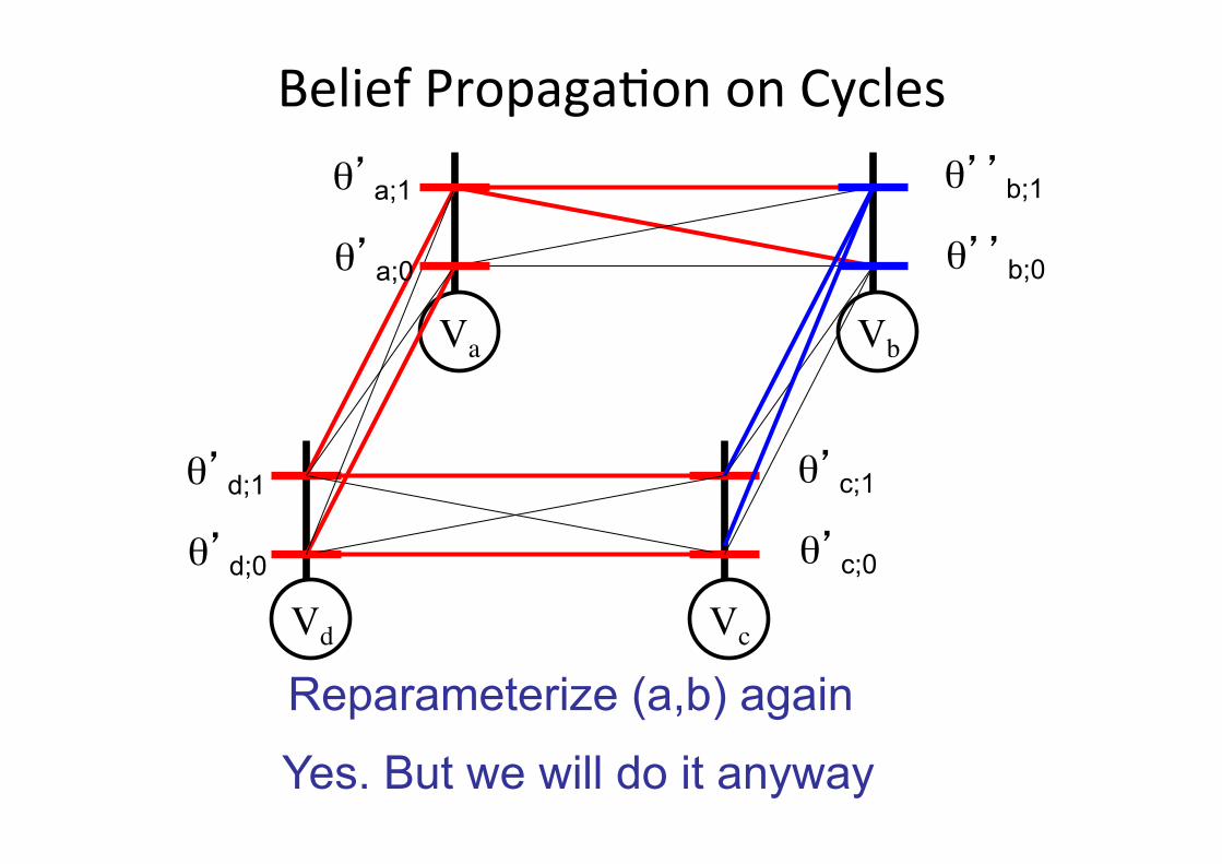
BeliefPropagaQononCycles
Va Vb
Vd Vc
θ’a;0
θ’a;1
θ’’b;0
θ’’b;1
θ’d;0
θ’d;1
θ’c;0
θ’c;1
Reparameterize (a,b) again
Yes. But we will do it anyway
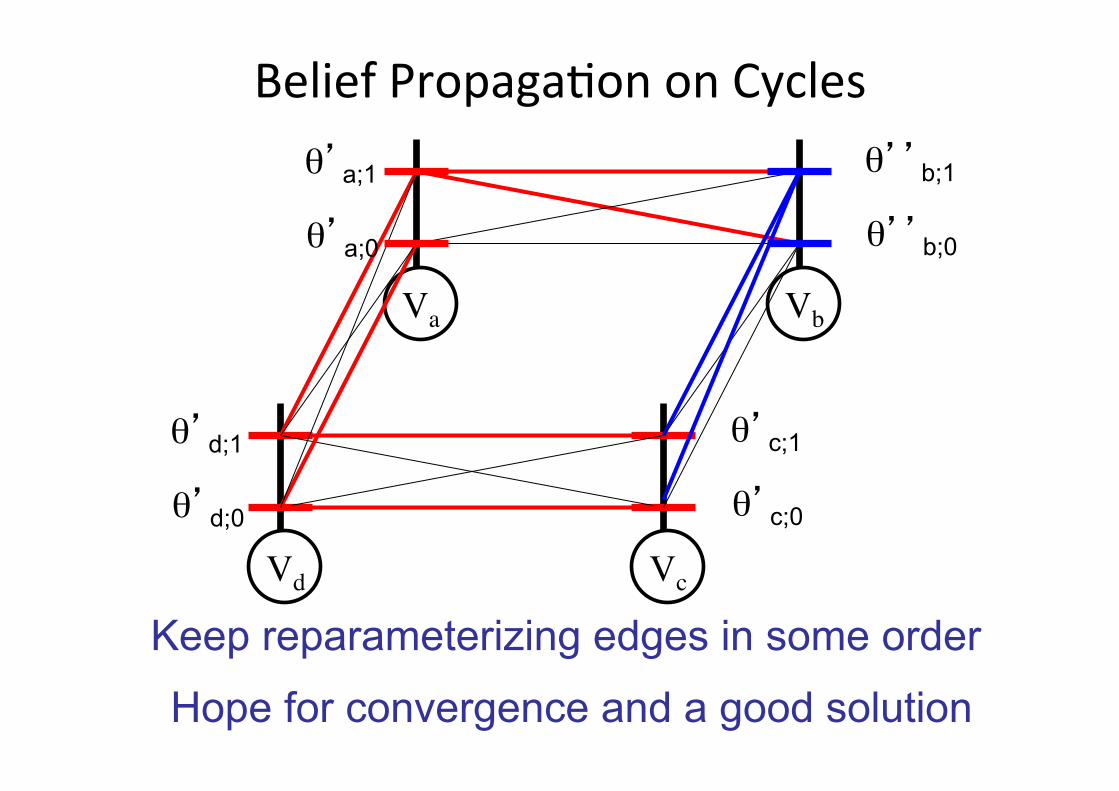
BeliefPropagaQononCycles
Va Vb
Vd Vc
θ’a;0
θ’a;1
θ’’b;0
θ’’b;1
θ’d;0
θ’d;1
θ’c;0
θ’c;1
Keep reparameterizing edges in some order
Hope for convergence and a good solution

Belief Propagation
• Generalizes to any arbitrary random field
• Complexity per iteration ?
O(|E||L|2) • Memory required ?
O(|E||L|)

Computational Issues of BP Complexity per iteration O(|E||L|2)
Special Pairwise Potentials θab;ik = wabd(|i-k|)
i - k
d
Potts i - k
d
Truncated Linear i - k
d
Truncated Quadratic
O(|E||L|) Felzenszwalb & Huttenlocher, 2004
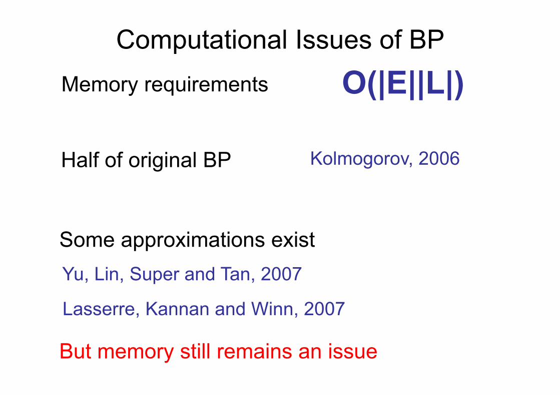
Computational Issues of BP Memory requirements O(|E||L|)
Half of original BP Kolmogorov, 2006
Some approximations exist
But memory still remains an issue
Yu, Lin, Super and Tan, 2007
Lasserre, Kannan and Winn, 2007
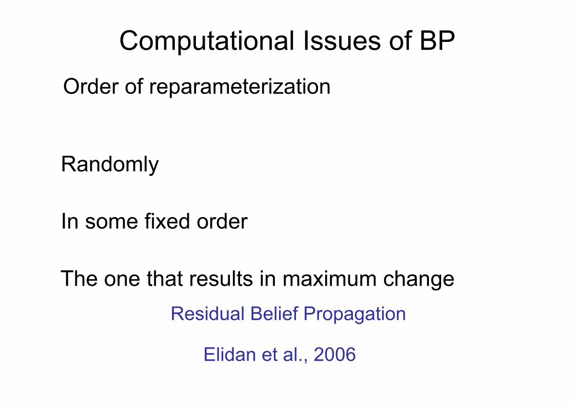
Computational Issues of BP Order of reparameterization
Randomly
Residual Belief Propagation
In some fixed order
The one that results in maximum change
Elidan et al., 2006
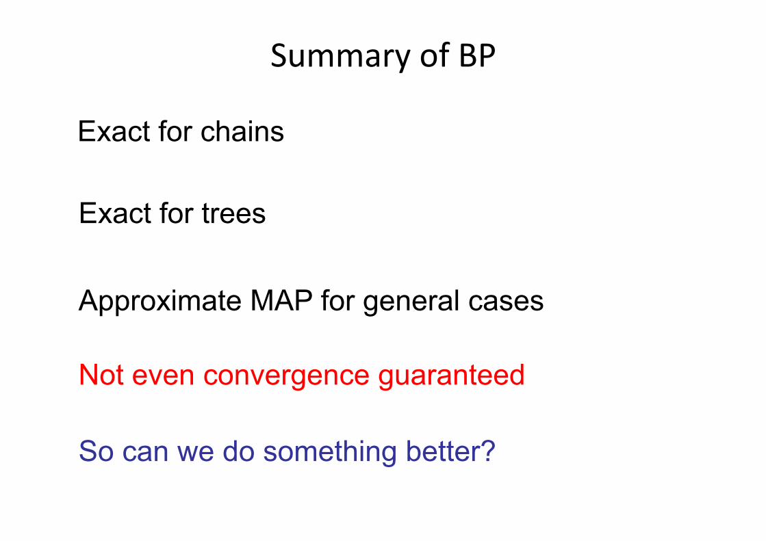
SummaryofBP
Exact for chains
Exact for trees
Approximate MAP for general cases
Not even convergence guaranteed
So can we do something better?

OtheralternaQves
• TRW, Dual decomposition methods
• Integer linear programming and relaxation
• Extensively studied - Schlesinger, 1976 - Koster et al., 1998, Chekuri et al., ’01, Archer et al., ’04 - Wainwright et al., 2001, Kolmogorov, 2006 - Globerson and Jaakkola, 2007, Komodakis et al., 2007 - Kumar et al., 2007, Sontag et al., 2008, Werner, 2008 - Batra et al., 2011, Werner, 2011, Zivny et al., 2014

Wheredowestand?
Chain/Tree, 2-label: Use BP
Chain/Tree, multi-label: Use BP
Grid graph: Use TRW, dual decomposition, relaxation

NoteonDynamicProgramming

DynamicProgramming(DP)
• DP≈“carefulbruteforce”
• DP≈recursion+memoizaQon+guessing
• Dividetheproblemintosubproblemsthatareconnectedtotheoriginalproblem
• Graphofsubproblemshastobeacyclic(DAG)
• Time=#subproblems·Qme/subproblem
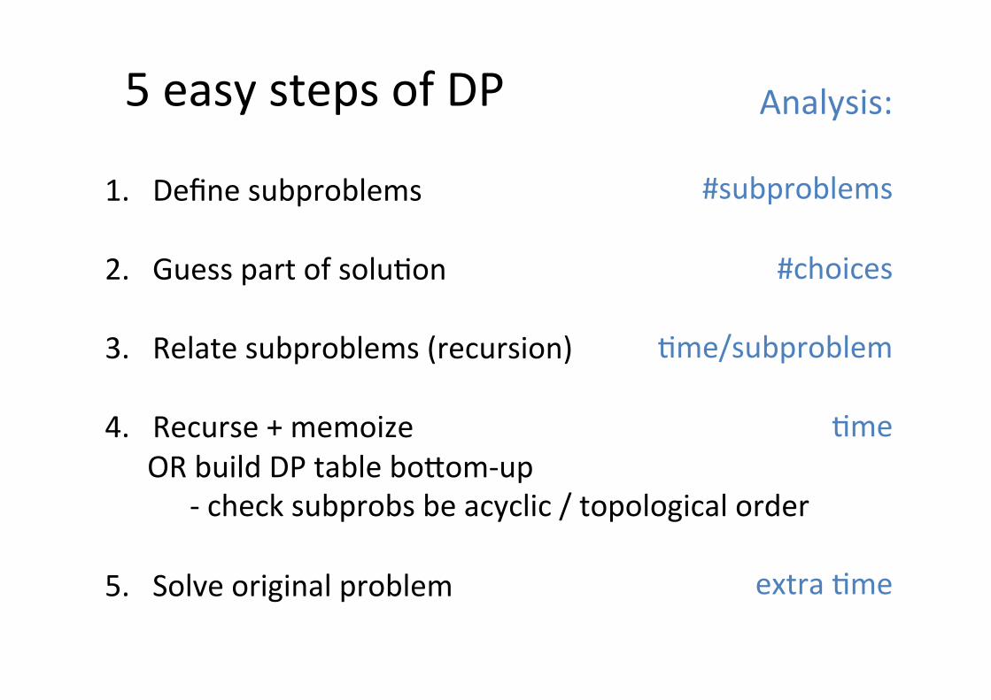
5easystepsofDP
1. Definesubproblems
2. GuesspartofsoluQon
3. Relatesubproblems(recursion)
4. Recurse+memoizeORbuildDPtablebo;om-up -checksubprobsbeacyclic/topologicalorder
5. Solveoriginalproblem
Analysis:
#subproblems
#choices
Qme/subproblem
Qme
extraQme
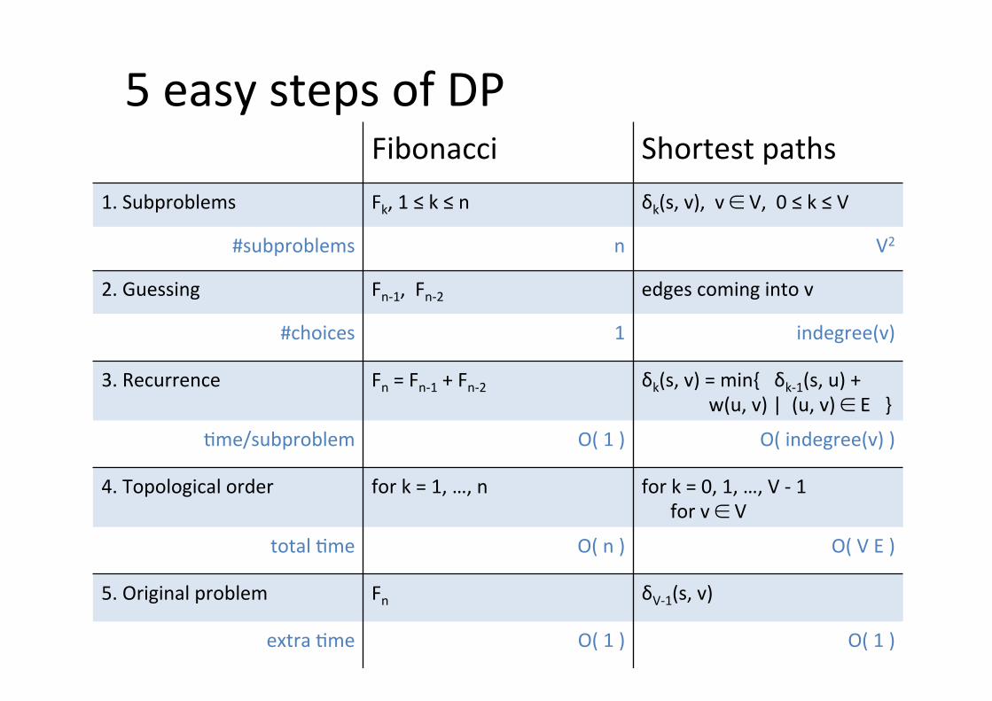
5easystepsofDPFibonacci Shortestpaths
1.Subproblems Fk,1≤k≤n δk(s,v),v∈V,0≤k≤V
#subproblems n V2
2.Guessing Fn-1,Fn-2 edgescomingintov
#choices 1 indegree(v)
3.Recurrence Fn=Fn-1+Fn-2 δk(s,v)=min{δk-1(s,u)+w(u,v)|(u,v)∈E}
Qme/subproblem O(1) O(indegree(v))
4.Topologicalorder fork=1,…,n fork=0,1,…,V-1forv∈V
totalQme O(n) O(VE)
5.Originalproblem Fn δV-1(s,v)
extraQme O(1) O(1)