Discrete approximation of quantum stochastic models

Discrete approximation of quantum stochastic modelsLuc Bouten and Ramon Van Handel Citation: Journal of Mathematical Physics 49, 102109 (2008); doi: 10.1063/1.3001109 View online: http://dx.doi.org/10.1063/1.3001109 View Table of Contents: http://scitation.aip.org/content/aip/journal/jmp/49/10?ver=pdfcov Published by the AIP Publishing Articles you may be interested in Using stochastic models calibrated from nanosecond nonequilibrium simulations to approximate mesoscaleinformation J. Chem. Phys. 130, 144908 (2009); 10.1063/1.3106225 Stochastic Models of Quantum Mechanics — A Perspective AIP Conf. Proc. 889, 106 (2007); 10.1063/1.2713450 A Stochastic Mechanics And Its Connection With Quantum Mechanics AIP Conf. Proc. 750, 361 (2005); 10.1063/1.1874587 Quantum stochastic differential equation for unstable systems J. Math. Phys. 41, 7220 (2000); 10.1063/1.1310357 Quantum stochastic models of two-level atoms and electromagnetic cross sections J. Math. Phys. 41, 7181 (2000); 10.1063/1.1289380

This article is copyrighted as indicated in the article. Reuse of AIP content is subject to the terms at: http://scitation.aip.org/termsconditions. Downloaded to IP: 193.0.65.67

On: Mon, 22 Dec 2014 09:50:35

http://scitation.aip.org/content/aip/journal/jmp?ver=pdfcov

http://oasc12039.247realmedia.com/RealMedia/ads/click_lx.ads/www.aip.org/pt/adcenter/pdfcover_test/L-37/578858469/x01/AIP-PT/CiSE_JMPArticleDL_121714/Awareness_LibraryF.jpg/47344656396c504a5a37344142416b75?x

http://scitation.aip.org/search?value1=Luc+Bouten&option1=author

http://scitation.aip.org/search?value1=Ramon+Van+Handel&option1=author

http://scitation.aip.org/content/aip/journal/jmp?ver=pdfcov

http://dx.doi.org/10.1063/1.3001109

http://scitation.aip.org/content/aip/journal/jmp/49/10?ver=pdfcov

http://scitation.aip.org/content/aip?ver=pdfcov

http://scitation.aip.org/content/aip/journal/jcp/130/14/10.1063/1.3106225?ver=pdfcov

http://scitation.aip.org/content/aip/journal/jcp/130/14/10.1063/1.3106225?ver=pdfcov

http://scitation.aip.org/content/aip/proceeding/aipcp/10.1063/1.2713450?ver=pdfcov

http://scitation.aip.org/content/aip/proceeding/aipcp/10.1063/1.1874587?ver=pdfcov

http://scitation.aip.org/content/aip/journal/jmp/41/11/10.1063/1.1310357?ver=pdfcov

http://scitation.aip.org/content/aip/journal/jmp/41/11/10.1063/1.1289380?ver=pdfcov

Discrete approximation of quantum stochastic modelsLuc Bouten1,a� and Ramon Van Handel2,b�

1Physical Measurement and Control 266-33, California Institute of Technology, Pasadena,California 91125, USA2Department of Operations Research and Financial Engineering, Princeton University,Princeton, New Jersey 08544, USA

�Received 16 July 2008; accepted 26 September 2008; published online 20 October 2008�

We develop a general technique for proving convergence of repeated quantuminteractions to the solution of a quantum stochastic differential equation. The wideapplicability of the method is illustrated in a variety of examples. Our main theo-rem, which is based on the Trotter–Kato theorem, is not restricted to a specificnoise model and does not require boundedness of the limit coefficients. © 2008American Institute of Physics. �DOI: 10.1063/1.3001109�

I. INTRODUCTION

It has been well established that the quantum stochastic equations introduced by Hudson andParthasarathy18 provide an essential tool in the theoretical description of physical systems, espe-cially those arising in quantum optics. The time evolution in these models is given by a unitarycocycle that solves a Hudson–Parthasarathy quantum stochastic differential equation �QSDE�.These unitaries define a flow, which is a quantum Markov process in the sense of Ref. 1, thatrepresents the Heisenberg time evolution of the observables of the physical system. Several au-thors have studied how quantum stochastic models can be obtained as a limit of fundamentalmodels in quantum field theory.2,15,9 This provides a sound justification for using quantum sto-chastic models to describe physical systems arising, e.g., in quantum optics.

In contrast to the limit theorems for field theoretic models, which are non-Markovian and havecontinuous time parameter, it is natural to ask whether QSDEs can be obtained as a limit ofdiscrete time quantum Markov chains. Classical counterparts of such results are ubiquitous inprobability theory and there is a variety of motivations �to be discussed further below� to studysuch limits. The first results on this topic date back to the work of Lindsay and Parthasarathy.26,21

In Ref. 26 it is shown that a particular class of repeated interaction models, where a physicalsystem is coupled to a spin chain, converge in a very weak sense �in matrix elements� to thesolution of a QSDE. A significant step forward was taken in Ref. 21 where Lindsay and Parthasa-rathy embedded a chain of finite-dimensional noise systems in the algebra of bounded operators onthe Fock space and showed strong convergence of the discrete flow to the flow obtained from aQSDE. Much later, Attal and Pautrat3 obtained similar results �in the special case of a spin chain�by showing that the discrete unitaries �rather than the flows� converge strongly to the solution ofa QSDE.

Independent of the previous work on the convergence of discrete chains, Holevo16,17 studieda very similar problem in his work on time-ordered exponentials in quantum stochastic calculus.The essence of Holevo’s approach is to define time-ordered stochastic exponentials as the limit ofdiscrete interaction models, where the role of the discrete noise is played by the increments in thefield operators �the discrete noise is thus infinite dimensional in this setting, in contrast to the

a�Electronic mail: [email protected]�Electronic mail: [email protected].

JOURNAL OF MATHEMATICAL PHYSICS 49, 102109 �2008�

49, 102109-10022-2488/2008/49�10�/102109/19/$23.00 © 2008 American Institute of Physics


On: Mon, 22 Dec 2014 09:50:35

http://dx.doi.org/10.1063/1.3001109

http://dx.doi.org/10.1063/1.3001109

finite-dimensional models considered by Lindsay and Parthasarathy21�. Despite the rather differentmotivation, the results of Holevo16,17 are strikingly similar to those obtained in the study of limitsof discrete interaction models, as has been pointed out by Gough.14

None of these results, however, are capable of dealing with the physically important case oflimit QSDEs with unbounded initial coefficients �a typical setting in, e.g., quantum optics�. Thisrestriction is inherent to the techniques used to prove these results, which rely on Dyson seriesexpansions and require boundedness of the coefficients. Moreover, each of the above results hasbeen proved separately in its own setting, while the similarity between these results stronglysuggests that they should be unified within a common framework.

The purpose of this paper is to introduce a general technique for proving convergence of asequence of discrete quantum Markov chains to the solution of a QSDE. Our approach does notrely on a Dyson series expansion but instead employs a form of the Trotter–Kato theorem. Thisallows us to deal with unbounded coefficients in a natural and transparent manner. In the simplercase where the limit coefficients and/or discrete noises are bounded, we obtain many of theprevious results as special cases of our general theorems. Moreover, the specific functional form ofthe limiting coefficients, obtained in Refs. 3, 16, and 14 by identifying a power series obtainedfrom the Dyson expansion, is effectively demystified: we will see that it is an immediate conse-quence of the scaling of the noise operators.

Our motivation for this work is twofold. First, the convergence of discrete quantum Markovchains to continuous ones is a fundamental problem in quantum probability theory. In classicalprobability theory such problems have been investigated for many decades, and the theory hasculminated in the well known work of Stroock and Varadhan �Ref. 30, Sec. 11.2�, Ethier andKurtz,10 and Kushner,20 among others. A similar systematic investigation was hitherto lacking inthe quantum probability literature. This paper presents one attempt to unify and extend the existingresults in this direction.

Second, we are motivated by practical problems in which one is specifically interested in theconvergence of discrete to continuous models. For example, certain laboratory experiments, e.g.,atomic beam experiments with a large flux of atoms, can be approximately modeled by quantumstochastic equations in the limit of large flux. Another application of independent interest is thedevelopment of numerical methods for quantum stochastic models. To perform tractable numericalsimulations, one is often forced to discretize, particularly in dynamical optimization problemswhich appear in the emerging field of quantum engineering,6 and convergence of the discretizedapproximations is a challenging topic. We were motivated in particular by the problem of dis-cretizing linear quantum systems, which play a special role in linear systems theory,19,25,24 but arenot covered by previous results as both the noise and the initial system are necessarily unbounded.

As compared to previous results, our approach is closest to the original method of Lindsay andParathasarathy.21 The simple uniform convergence result �Ref. 21, Proposition 3.3� is replaced inour setting by a variant of the Trotter–Kato theorem,10 which allows us to deal with the analyticcomplications inherent to the case of unbounded coefficients. We also work directly with theunitary evolution rather than with the flow. The Trotter–Kato theorem allows us to obtain conver-gence by studying generators and exploits in a fundamental way the Markov property of both theapproximate and the limit evolutions.

Techniques to obtain convergence for QSDEs by studying generators were introduced byFagnola12 and Chebotarev8 �using resolvents� and by Lindsay and Wills22,23 �using the Trotter–Kato theorem�. We have previously applied related techniques to obtain general results on singularperturbation problems for quantum stochastic models.5,7 The application of this type of techniqueto obtain the convergence of discrete quantum models is new.

The remainder of this paper is organized as follows. In Sec. II we introduce the class ofdiscrete interaction models and limit models which will be of interest throughout the paper, andwe state our main results. The main theorem is a generalization of the Trotter–Kato theorem toquantum stochastic models and is generally applicable. We also introduce a more restricted family

102109-2 L. Bouten and R. Van Handel J. Math. Phys. 49, 102109 �2008�


On: Mon, 22 Dec 2014 09:50:35

of discrete models for which the conditions of this result can be verified explicitly. Section IIIdevelops a variety of known and new examples using our results. Finally, Sec. IV is devoted to theproofs of our results.

II. MAIN RESULTS

In Secs. II A–II D, we first define the class of models that we will consider and introduce thenecessary assumptions. This is followed by the statement of our main results. The proofs of ourmain results are contained in Sec. IV below.

A. The limit model

Throughout this paper we let H, the initial space, be a separable �complex� Hilbert space. Wedenote by F=�s�L2�R+ ;Cn�� the symmetric Fock space with multiplicity n�N �i.e., the one-particle space is Cn � L2�R+��L2�R+ ;Cn�� and by e�f�, f �L2�R+ ;Cn� the exponential vectors in F.The annihilation, creation, and gauge processes on F, as well as their ampliations to H � F, willbe denoted as At

i, Ati†, and �t

ij, respectively �the channel indices are relative to the canonical basisof Cn�. Moreover, we will fix once and for all a dense domain D�H and a dense domain ofexponential vectors E=span�e�f� : f �S��F, where S�L2�R+ ;Cn��Lloc

� �R+ ;Cn� is an admis-sible subspace in the sense of Hudson–Parthasarathy18 which is presumed to contain at least allsimple functions. An introduction to these concepts �using a similar notation to the one used here�can be found in Ref. 4 and we refer to Refs. 18 and 27 for a detailed description of quantumstochastic calculus.

Consider a QSDE of the form

dUt = Ut�i,j=1

n

�Nij − �ij�d�tij +

i=1

n

MidAti† +

i=1

n

LidAti + Kdt , �1�

where U0= I and the quantum stochastic integrals are defined relative to the domain D�̄E �forsimplicity, we will use the same notation for operators on H or on F and for their ampliations toH � F�. Under certain conditions to be introduced below, the solution of this equation describesthe time evolution of quantum stochastic models such as those used in quantum optics. Thepurpose of this paper is to prove that the solution of this equation may be approximated byappropriately chosen discrete interaction models. The approximating models will be defined inSec. II B.

Denote by �t :L2� � t ,� � ;Cn�→L2�R+ ;Cn� the canonical shift �t f�s�= f�t+s� and by �t :F�t�→F its second quantization �here F�F�t� � F�t� denotes the usual continuous tensor productdecomposition�. Recall that an adapted process �Ut : t�0� on H � F is called a unitary cocycle ifUt is unitary for all t�0, t�Ut is strongly continuous, and Us+t=Us�I � �s

�Ut�s�, where I� �s

�Ut�s is viewed as an operator on F�s� � �H � F�s��H � F. The following condition willalways be presumed to be in force.

Condition 1: The operators K , Li , Mi , and Nij , defined on the domain D , are such that theHudson–Parthasarathy equation (1) possesses a unique solution �Ut : t�0� which extends to aunitary cocycle on H � F .

Remark 1: When the coefficients K, Li, Mi, and Nij are bounded, it is well known18 thatCondition 1 holds true if and only if the following algebraic relations are satisfied:

K + K� = − i=1

n

LiLi�, Mi = −

j=1

n

NijLj�,

102109-3 Discrete approximation in quantum stochastics J. Math. Phys. 49, 102109 �2008�


On: Mon, 22 Dec 2014 09:50:35

j=1

n

NmjN�j� =

j=1

n

Njm� Nj� = �m�.

Remarks on the verification of Condition 1 in the unbounded case can be found in Ref. 7.Remark 2: We have chosen the left Hudson–Parthasarathy equation �1� rather than the more

familiar right equation where the solution is placed to the right of the coefficients. This means thatthe Schrödinger evolution of a state vector ��H � F is given by Ut

��, etc. The reason for thischoice is that for equations with unbounded coefficients, it is generally much easier to prove theexistence of a unique cocycle solution for the left equation than for the right equation �see, e.g.,Refs. 11 and 22�. As we will ultimately prove convergence of discrete evolutions to Ut

�, there is noloss of generality in working with the more tractable left equations. If we wish to begin with a welldefined right equation �as is more natural when the coefficients are bounded�, our results can beimmediately applied to the Hudson–Parthasarathy equation for its adjoint.

B. The discrete approximations

A discrete interaction model describes the repeated interaction of an initial system with inde-pendent copies of an external noise source. Given an initial Hilbert space H� and a noise Hilbertspace K�, a single interaction is described by a unitary operator R� on H� � K�. To describe

repeated interactions, we work on the Hilbert space H� � � NK� on which we define the naturalisomorphism,

k:�K��k−1�� H� � �

NK� → H� � �

NK�,

as k��k−1� � � ��k��= � ��k−1� � ��k��. We now define recursively R0�= I and

Rk�� k−1� � �k � ��k+1�� = Rk−1� k��k−1� � R�� k� � ��k+1��

for k�N, where ��k−1� � �k � ��k+1�� K��k−1� � K� � � NK�� NK� and �H�. This is pre-cisely the discrete counterpart of a unitary cocycle. Note that the order of multiplication in therecursion for Rk� matches the choice of the left Hudson–Parthasarathy equation above �i.e., Rk�

�� isthe Schrödinger evolution, see Remark 2�.

The purpose of this paper is to prove that the solution of the Hudson–Parthasarathy equation�1� can be approximated by a sequence of discrete interaction models with decreasing time step. Inorder to study this problem, we will embed our discrete interaction models in the limit Hilbertspace H � F. This allows us to prove strong convergence of the embedded discrete cocycles to thesolution of Eq. �1�. The precise way in which the embedding is done does not affect the proof ofour main result; we therefore proceed in a general fashion by defining a fixed but otherwisearbitrary sequence of discrete interaction models which are already embedded into the limit Hil-bert space �this avoids, without any loss of generality, the notational burden of introducing sepa-rate Hilbert spaces and embedding maps for every discrete approximation�. As a special case ofthis general construction, we will introduce in Sec. II D below an interesting class of discreteinteraction models for which the embedding is made explicit.

We proceed to introduce the embedded discrete interaction models. For every k�N, we willdefine a discrete interaction model with time step1 2−k �the ultimate goal being to take the limit as

k→��. By its continuous tensor product property, the Fock space is isomorphic to F� � NF�2−k�,

where each component F�2−k� represents a consecutive time slice of length 2−k. Ourdiscrete interaction models will be embedded as repeated interactions with consecutive time slices

1This choice is only made to keep our notation manageable and is by no means a restriction of the method.



On: Mon, 22 Dec 2014 09:50:35

of the field. Let us make this precise: the following notations will be used throughout the paper.Let Hk�H be the initial Hilbert space and let Kk�F�2−k� be the noise Hilbert space for the

interaction model with time step 2−k. We will write

Fk = �N

Kk � �N

F�2−k� � F .

We now introduce a unitary operator Rk on Hk � Kk which describes the interaction in a singletime step, and we extend Rk to H � F by setting Rk�=� for �� Hk � Kk � F�2−k��. We nowdefine recursively Rt

k= I for t� �0,2−k� and

Rtk = R��−1�2−k

k �I � ��−1�2−k� Rk��−1�2−k� for t � ��2−k,�� + 1�2−k�, � � N ,

where I � ��2−k� Rk��2−k is viewed as an operator on F��2−k� � �H � F��2−k��H � F. In other

words, the discrete evolution Rtk is an adapted unitary process which is piecewise constant on

consecutive intervals of length 2−k, and an interaction between the initial system and the next fieldslice occurs at the beginning of every interval. Our goal is to prove that Rt

k converges as k→� tothe solution Ut of Eq. �1�.

Remark 3: This model coincides precisely with the discrete interaction model defined aboveif we choose H�=Hk, K�=Kk, R�=Rk, and R��=R�2−n

k .

C. A general limit theorem

Before we proceed to the statement of our main result, we introduce certain families ofsemigroups which will play a central role in our approach.

Lemma 1: For k�N and � ,��F�2−k� , define Rk;�� :H→H such that

�u,Rk;��v� = � −1 � −1�u � �,Rkv � �� ∀ u,v � H .

Then Rk;�� is a contraction on H and

�u,�Rk;��t2k�v� = � −N2k � −N2k

�u � ��N2k,Rt

kv � ��N2k�

for all u ,v�H and t� �0,N� , N�N .Proof. This follows directly from the unitarity of Rk and the definition of Rt

k. �

The following counterpart for the limit equation �1� is proved in Ref. 7, Lemma 1.Lemma 2: For � , �Cn , define Tt

� :H→H such that

�u,Tt� v� = e−��2+� �2�t/2�u � e��I�0,t��,Utv � e� I�0,t�� ∀ u,v � H, t � 0.

Then Tt� is a strongly continuous contraction semigroup on H , and the generator L� of this

semigroup satisfies Dom�L� ��D such that for u�D

L� u = �i,j=1

n

�i�Nij j +

i=1

n

�i�Mi +

i=1

n

Li i + K −��2 + � �2

2�u .

The reason to focus on the semigroups associated to our models is that we will seek conditionsfor convergence of the discrete approximations in terms of the generators L� . As the latter isexpressed directly in terms of the coefficients of the limit equation �1�, such conditions cantypically be verified in a straightforward manner and do not require us to work directly with thesolution Ut of that equation.

The following is the main result of this paper. The theorem bears a strong resemblance to theTrotter–Kato theorem for contraction semigroups, and the latter does indeed form the foundationof the proof. The proof of the theorem is given in Sec. IV.

Theorem 1: Assume that Condition 1 holds, and let D� �Dom�L� � be a core for L� ,� , �Cn . Then the following conditions are equivalent.



On: Mon, 22 Dec 2014 09:50:35

�1� For all � , �Cn , u�D� there exist uk�H and �k ,�k�F�2−k� so that

uk ——→k→�

u, ��k��2k——→

k→�

e��I�0,1��, ��k��2k——→

k→�

e� I�0,1�� ,

and

2k�Rk;�k�k− I�uk ——→

k→�

L� u .

�2� For every T�� and ��H � F

limk→�

sup0�t�T

Rtk�� − Ut

�� = 0.

Remark 4: As was pointed out to us by a referee, this theorem could also be stated outside theframework of QSDEs. Indeed, a careful reading of the proof reveals that one may dispose ofCondition 1 entirely and assume only that Ut is any unitary cocycle on H � F. The theorem is themost powerful, however, when the generators L� admit an explicit expression in terms of theparameters of the limit model. This is the case, in particular, when Condition 1 is satisfied and Dis a core for all L� , � , �C. We can then choose D� �D, with the important consequence thatthis puts the explicit expression for L� in Lemma 2 at our disposal. This will be the case in all ourexamples. Typically existence and uniqueness proofs for the solution of �1� already imply that Dis a core for L� , see, e.g., Refs. 11, 22, and 7 �Remark 4� for further comments.

Remark 5: The assumption in Condition 1 that Ut is a unitary cocycle can be weakenedsomewhat. In the absence of this assumption, one may still prove the implication 1⇒2 providedthat strong convergence uniformly on compact intervals is replaced by weak convergence of Rt

k toUt for every time t. We have chosen to concentrate on the unitary case, as it is the relevant one forphysical applications and admits a much stronger result.

D. A class of discrete interactions

Theorem 1 is a very general result which allows us to infer the convergence of a sequence ofdiscrete interaction models to the solution of the Hudson–Parthasarathy equation �1�. The verifi-cation of the conditions of the theorem requires additional work, however, and the form of thelimit coefficients depends on the choice of the discrete interactions Rk. In this section we introducea special class of discrete interaction models �with Hk=H� for which the conditions of Theorem1 can be verified explicitly. In particular, we obtain explicit expressions for the limit coefficients.It should be noted that this class of discrete interaction models is physically natural, and we willencounter several concrete examples in Sec. III.

Let K be a fixed Hilbert space and suppose that we are given a sequence of bounded operators�k :K→F�2−k� which are partially isometric in the following sense:

�k��k = IK, �k�k� = PKk for all k, where Kkª ran �k.

Here PKk is the orthogonal projection onto Kk and IK is the identity on K. The same space K willplay the role of the noise Hilbert space for every discrete interaction model Rk �k�N� after beingisometrically embedded into the limit Hilbert space by the embedding maps �k. As we will see,the choice to work with a fixed noise space prior to embedding is convenient due to the fact thatthe limit coefficients can be expressed in terms of the matrix elements of certain operators onH � K.

We now define the discrete models. Let F1 , . . . ,F�, G1 , . . . ,Gm, and H1 , . . . ,Hr �� ,m ,r�N� bebounded self-adjoint operators on H, and let �1 , . . . ,��, �1 , . . . ,�m, and �1 , . . . ,�r be �not neces-sarily bounded� self-adjoint operators on K. Define



On: Mon, 22 Dec 2014 09:50:35

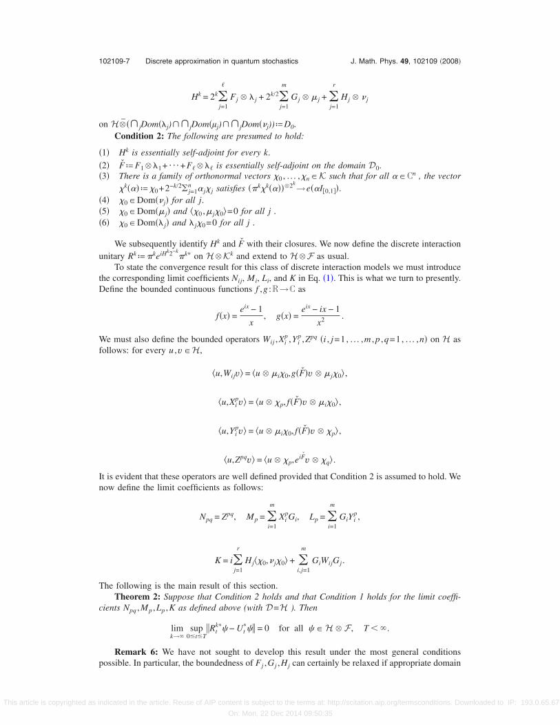
Hk = 2kj=1

�

Fj � � j + 2k/2j=1

m

Gj � � j + j=1

r

Hj � � j

on H�̄��jDom��j)��jDom�µj)��jDom��j))ªD0.Condition 2: The following are presumed to hold:

�1� Hk is essentially self-adjoint for every k.

�2� F̌ªF1 � �1+ ¯ +F� � �� is essentially self-adjoint on the domain D0.�3� There is a family of orthonormal vectors �0 , . . . ,�n�K such that for all ��Cn , the vector

�k��ª�0+2−k/2 j=1n � j� j satisfies ��k�k��2k→e��I�0,1��.

�4� �0�Dom�� j� for all j.�5� �0�Dom�� j� and ��0 ,� j�0�=0 for all j .�6� �0�Dom�� j� and � j�0=0 for all j .

We subsequently identify Hk and F̌ with their closures. We now define the discrete interactionunitary Rk

ª�keiHk2−k�k� on H � Kk and extend to H � F as usual.

To state the convergence result for this class of discrete interaction models we must introducethe corresponding limit coefficients Nij, Mi, Li, and K in Eq. �1�. This is what we turn to presently.Define the bounded continuous functions f ,g :R→C as

f�x� =eix − 1

x, g�x� =

eix − ix − 1

x2 .

We must also define the bounded operators Wij ,Xip ,Yi

p ,Zpq �i , j=1, . . . ,m , p ,q=1, . . . ,n� on H asfollows: for every u ,v�H,

�u,Wijv� = �u � �i�0,g�F̌�v � � j�0� ,

�u,Xipv� = �u � �p, f�F̌�v � �i�0� ,

�u,Yipv� = �u � �i�0, f�F̌�v � �p� ,

�u,Zpqv� = �u � �p,eiF̌v � �q� .

It is evident that these operators are well defined provided that Condition 2 is assumed to hold. Wenow define the limit coefficients as follows:

Npq = Zpq, Mp = i=1

m

XipGi, Lp =

i=1

m

GiYip,

K = ij=1

r

Hj��0,� j�0� + i,j=1

m

GiWijGj .

The following is the main result of this section.Theorem 2: Suppose that Condition 2 holds and that Condition 1 holds for the limit coeffi-

cients Npq ,Mp ,Lp ,K as defined above (with D=H ). Then

limk→�

sup0�t�T

Rtk�� − Ut

�� = 0 for all � � H � F, T � � .

Remark 6: We have not sought to develop this result under the most general conditionspossible. In particular, the boundedness of Fj ,Gj ,Hj can certainly be relaxed if appropriate domain



On: Mon, 22 Dec 2014 09:50:35

assumptions are introduced, and the proof of the present result is then readily extended. We havechosen to restrict to the bounded case as the treatment of this case is particularly transparent, andwe have not found one single choice of domain conditions in the unbounded case which covers allexamples of interest in that setting �particularly straightforward extensions can be found wheneither Fj =0 for all j, or when only the Gj are bounded�. An illustrative example with unboundedcoefficients is developed in Sec. III by appealing directly to Theorem 1.

One might worry about the well-posedness of Theorem 2 as the limit coefficientsNpq ,Mp ,Lp ,K depend on our choice for �0 , . . . ,�n. For completeness, we provide the followingsimple lemma whose proof can be found in Sec. IV.

Lemma 3: Define �k�� as in Condition 2 (which we presume to be in force). Suppose that�̃0 , . . . , �̃n�K is another orthonormal family such that for every ��Cn,

�̃k�� ª �̃0 + 2−k/2j=1

n

� j�̃ j satisfies ��k�̃k��2k——→

k→�

e��I�0,1�� .

Then there is a ��R such that �̃ j =ei�� j for all j .Finally, it should be noted that Condition 1 imposes stronger assumptions on the noise opera-

tors � j and � j than is evident from Condition 2. The following lemma provides explicit assump-tions which guarantee that Condition 1 holds for the coefficients Npq ,Mp ,Lp ,K as defined in thissection. The proof is given in Sec. IV.

Lemma 4: Define S=span��1 , . . . ,�n� , and suppose that � j�0�S for all j . Suppose more-over that S�Dom�� j� and that � jS�S for all j . Then the limit coefficients Npq ,Mp ,Lp ,K satisfyCondition 1.

Remark 7: It is not difficult to construct examples of discrete interaction models where thelimit coefficients Npq ,Mp ,Lp ,K do not satisfy the Hudson–Parthasarathy conditions in Remark 1.In this case, our proofs may be modified to show that Rt

k nonetheless converges weakly to thesolution Ut of Eq. �1� with coefficients Npq ,Mp ,Lp ,K as defined in this section. However, in thiscase the limit evolution Ut will not be unitary, so that the physical relevance of such a result israther limited.

III. EXAMPLES

We illustrate our results using four examples. The first two examples reproduce the results ofAttal and Pautrat3 and Holevo.16 The third example, that of a linear quantum system, possessesboth unbounded noise operators and unbounded initial coefficients. Finally, the fourth exampleshows that we may simultaneously approximate the noise and the initial coefficients, as is oftenuseful in numerical simulations.

Until further notice H is a fixed Hilbert space. Note that for sake of example, all our modelslive in the Fock space with unit multiplicity n=1. The extension to multiple channels is entirelystraightforward and leads only to complication of the notation.

A. Spin chain models

Define K=C2 and denote the canonical basis of C2 as ��0 ,�1�. The noise Hilbert space is thusthat of a single spin. We embed the spin into the Fock space by defining the embedding map�k :K→F�2−k� through

�k�0 = e�0� = 1 � �p=1

�

0, �k�1 = 0 � 2k/2I�0,2−k� � �p=2

�

0

�here I�0,2−k� is the indicator function on the interval �0,2−k��. We now define bounded self-adjointoperators �, �1, and �2 on K as matrices with respect to the canonical basis:



On: Mon, 22 Dec 2014 09:50:35

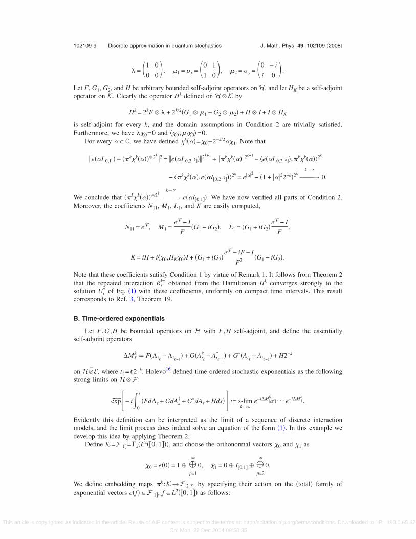
� = �1 0

0 0�, �1 = �x = �0 1

1 0�, �2 = �y = �0 − i

i 0� .

Let F, G1, G2, and H be arbitrary bounded self-adjoint operators on H, and let HK be a self-adjointoperator on K. Clearly the operator Hk defined on H � K by

Hk = 2kF � � + 2k/2�G1 � �1 + G2 � �2� + H � I + I � HK

is self-adjoint for every k, and the domain assumptions in Condition 2 are trivially satisfied.Furthermore, we have ��0=0 and ��0 ,�i�0�=0.

For every ��C, we have defined �k��=�0+2−k/2��1. Note that

e��I�0,1�� − ��k�k��2k 2 = e��I�0,2−k�� 2k+1

+ �k�k�� 2k+1− �e��I�0,2−k��,�k�k��2k

− ��k�k��,e��I�0,2−k��2k= e��2 − �1 + ��22−k�2k

——→k→�

0.

We conclude that ��k�k��2k——→

k→�

e��I�0,1��. We have now verified all parts of Condition 2.Moreover, the coefficients N11, M1, L1, and K are easily computed,

N11 = eiF, M1 =eiF − I

F�G1 − iG2�, L1 = �G1 + iG2�

eiF − I

F,

K = iH + i��0,HK�0�I + �G1 + iG2�eiF − iF − I

F2 �G1 − iG2� .

Note that these coefficients satisfy Condition 1 by virtue of Remark 1. It follows from Theorem 2that the repeated interaction Rt

k� obtained from the Hamiltonian Hk converges strongly to thesolution Ut

� of Eq. �1� with these coefficients, uniformly on compact time intervals. This resultcorresponds to Ref. 3, Theorem 19.

B. Time-ordered exponentials

Let F ,G ,H be bounded operators on H with F ,H self-adjoint, and define the essentiallyself-adjoint operators

�M�kª F��t�

− �t�−1� + G�At�

† − At�−1

† � + G��At�− At�−1

� + H2−k

on H�̄E, where t�=�2−k. Holevo16 defined time-ordered stochastic exponentials as the followingstrong limits on H � F:

exp��− i�0

t

�Fd�s + GdAs† + G�dAs + Hds��ª s-lim

k→�e−i�M�t2k�

k¯ e−i�M1

k.

Evidently this definition can be interpreted as the limit of a sequence of discrete interactionmodels, and the limit process does indeed solve an equation of the form �1�. In this example wedevelop this idea by applying Theorem 2.

Define K=F�1�=�s�L2��0,1��, and choose the orthonormal vectors �0 and �1 as

�0 = e�0� = 1 � �p=1

�

0, �1 = 0 � I�0,1� � �p=2

�

0.

We define embedding maps �k :K→F�2−k� by specifying their action on the �total� family ofexponential vectors e�f��F�1�, f �L2��0,1�� as follows:



On: Mon, 22 Dec 2014 09:50:35

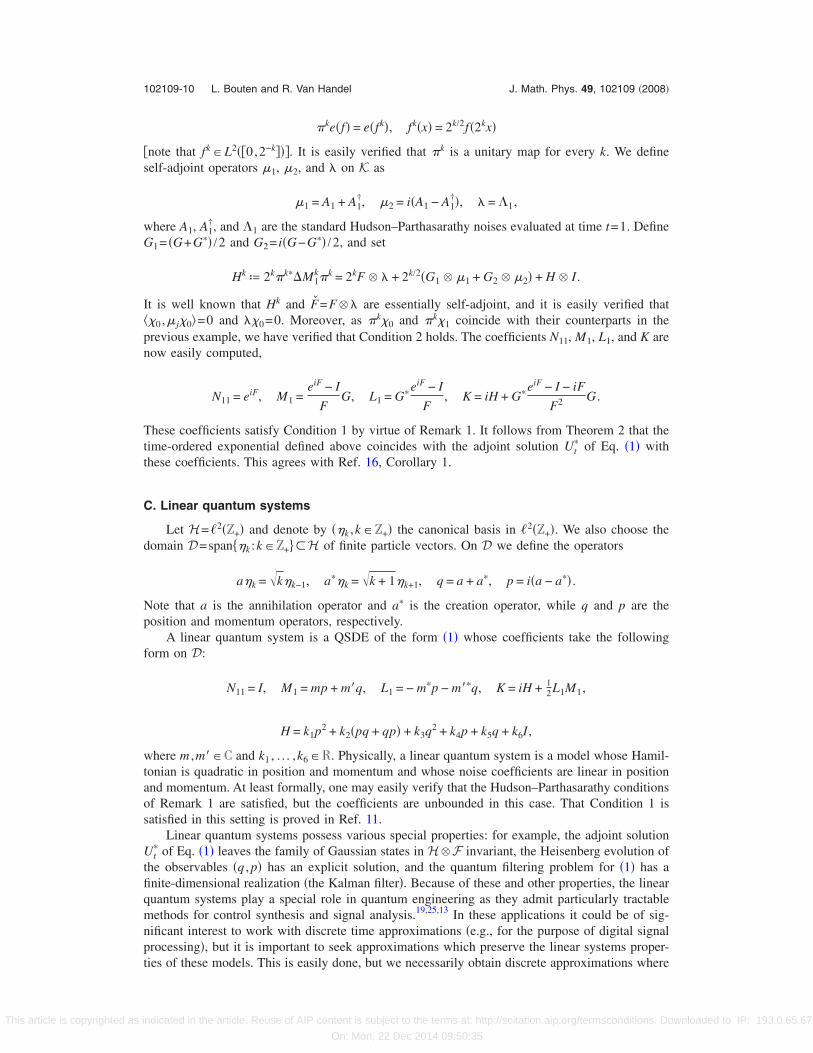
�ke�f� = e�fk�, fk�x� = 2k/2f�2kx�

�note that fk�L2��0,2−k��. It is easily verified that �k is a unitary map for every k. We defineself-adjoint operators �1, �2, and � on K as

�1 = A1 + A1†, �2 = i�A1 − A1

†�, � = �1,

where A1, A1†, and �1 are the standard Hudson–Parthasarathy noises evaluated at time t=1. Define

G1= �G+G�� /2 and G2= i�G−G�� /2, and set

Hkª 2k�k��M1

k�k = 2kF � � + 2k/2�G1 � �1 + G2 � �2� + H � I .

It is well known that Hk and F̌=F � � are essentially self-adjoint, and it is easily verified that��0 ,� j�0�=0 and ��0=0. Moreover, as �k�0 and �k�1 coincide with their counterparts in theprevious example, we have verified that Condition 2 holds. The coefficients N11, M1, L1, and K arenow easily computed,

N11 = eiF, M1 =eiF − I

FG, L1 = G�

eiF − I

F, K = iH + G�

eiF − I − iF

F2 G .

These coefficients satisfy Condition 1 by virtue of Remark 1. It follows from Theorem 2 that thetime-ordered exponential defined above coincides with the adjoint solution Ut

� of Eq. �1� withthese coefficients. This agrees with Ref. 16, Corollary 1.

C. Linear quantum systems

Let H=�2�Z+� and denote by ��k ,k�Z+� the canonical basis in �2�Z+�. We also choose thedomain D=span��k :k�Z+��H of finite particle vectors. On D we define the operators

a�k = �k�k−1, a��k = �k + 1�k+1, q = a + a�, p = i�a − a�� .

Note that a is the annihilation operator and a� is the creation operator, while q and p are theposition and momentum operators, respectively.

A linear quantum system is a QSDE of the form �1� whose coefficients take the followingform on D:

N11 = I, M1 = mp + m�q, L1 = − m�p − m��q, K = iH + 12L1M1,

H = k1p2 + k2�pq + qp� + k3q2 + k4p + k5q + k6I ,

where m ,m��C and k1 , . . . ,k6�R. Physically, a linear quantum system is a model whose Hamil-tonian is quadratic in position and momentum and whose noise coefficients are linear in positionand momentum. At least formally, one may easily verify that the Hudson–Parthasarathy conditionsof Remark 1 are satisfied, but the coefficients are unbounded in this case. That Condition 1 issatisfied in this setting is proved in Ref. 11.

Linear quantum systems possess various special properties: for example, the adjoint solutionUt

� of Eq. �1� leaves the family of Gaussian states in H � F invariant, the Heisenberg evolution ofthe observables �q , p� has an explicit solution, and the quantum filtering problem for �1� has afinite-dimensional realization �the Kalman filter�. Because of these and other properties, the linearquantum systems play a special role in quantum engineering as they admit particularly tractablemethods for control synthesis and signal analysis.19,25,13 In these applications it could be of sig-nificant interest to work with discrete time approximations �e.g., for the purpose of digital signalprocessing�, but it is important to seek approximations which preserve the linear systems proper-ties of these models. This is easily done, but we necessarily obtain discrete approximations where



On: Mon, 22 Dec 2014 09:50:35

both the initial system coefficients and the discrete noises are unbounded. In this example we willprove the convergence of such unbounded discrete approximations by appealing directly to ourmain theorem 1.

We begin, however, by setting up our discrete models as in Sec. II D. Let K=�2�Z+�, andchoose an embedding �k :K→F�2−k� by setting

�k�0 = 1 � �p=1

�

0, �k�� = �p=0

�−1

0 � �2k/2I�0,2−k��

p=�+1

�

0 �� N� .

If we define �k��ª�0+2−k/2��1 for ��C, then we find precisely as in the previous examplesthat ��k�k��2k→e��I�0,1�� as k→�.

Let us now define on D�̄D the operators

Hk = H � I − i�M1 � a� + L1 � a�2k/2.

One may verify that Hk is symmetric and that D�̄D is a domain of analytic vectors for Hk, so thatin particular Hk is essentially self-adjoint for every k �Ref. 28 Sec. X.6�. We will subsequentlyidentify these operators with their closures. Note that the Hamiltonian Hk is quadratic in the familyof position and momentum operators of the initial system and of the discrete noise; therefore thediscrete interaction model is itself a �discrete time� linear system, and it therefore possesses all theassociated desirable properties.

We now define the discrete interaction unitary Rk on H � F from the Hamiltonian Hk as inSec. II D. We will use Theorem 1 to prove that

limk→�

sup0�t�T

Rtk�� − Ut

�� = 0 for all � � H � F, T � � ,

where Ut is the solution of Eq. �1� with the coefficients N11, M1, L1, and K defined above. Notethat Theorem 2 does not apply as the initial coefficients are unbounded, but we may essentiallyrepeat the proof of that theorem with minor modifications to obtain the present result. To this end,we begin by noting that D is a core for L� �� , �C� by the analytic vector theorem �see Ref. 7,Remark 4�. Let us fix � , �C and define �k=�k�k�� and �k=�k�k� �. By Theorem 1, it sufficesto prove that

2k�Rk;�k�k− I�u − L� u ——→

k→�

0

for every u�D. We now proceed as follows. Fix u�D, and note that using the trivial identitieseix=1+ f�x�x=1+ ix+g�x�x2, we can write

eiHk2−ku � �� = �I + 2−kf�Hk2−k�Hk�u � �� = �I + iHk2−k + 2−2kg�Hk2−k��Hk�2�u � ��.

Here we have used the spectral theorem and the fact that u � ��Dom��Hk�p� for every � , p �seethe proof of Theorem 2 for a more precise argument�. Therefore

�v � �k��,2k�eiHk2−k− I�u � �k� ��

= i�v,Hu� − �v � �0,g�Hk2−k��M1 � a� + L1 � a�M1u � �1� − i��v � �1, f�Hk2−k�M1u � �1�

− i�v � �0, f�Hk2−k��M1 � a� + L1 � a�u � �1� + ��v � �1,�eiHk2−k− I�u � �1�

+ O� v 2−k/2� .

A straightforward computation shows that



On: Mon, 22 Dec 2014 09:50:35

supv�H v �1

��v � �k��,2k�eiHk2−k− I�u � �k� �� − �v,��M1 + L1 + K�u�� ——→

k→�

0,

where we have used that f�Hk2−k�→ iI, g�Hk2−k�→−�1 /2�I, and eiHk2−k→ I strongly as k→� byRef. 29, Theorems VIII.20 and VIII.25. As in the proof of Theorem 2 below, it follows readily that 2k�Rk;�k�k

− I�u−L� u →0.

D. Finite-dimensional approximations

In the previous examples we have approximated the QSDE �1� by constructing discrete inter-action models whose interaction unitary Rk lives on the Hilbert space H � Kk. Even though theFock space F is infinite dimensional, we have seen that we may choose finite-dimensional discretenoise spaces as simple as Kk�C2. In numerical applications, however, we typically wish to go onestep further and approximate also the initial space H �which is often infinite dimensional� by afinite-dimensional space Hk. The discrete interaction models then live entirely on the finite-dimensional Hilbert spaces Hk � Kk, as is desirable for numerical implementation. We would liketo establish that these discrete models converge to the solution of the limit equation �1� when wesimultaneously let the time step go to zero and let the initial space dimension go to infinity. Wewill now show in a toy example that this problem fits into the setting of Theorem 1.

We will discretize the noise essentially as in the example of Sec. III A, but let us directlyembed the discrete models �rather than work with the embedding maps �k� to simplify the nota-tion. For every k�N, define the vectors �0

k ,�1k �F�2−k� as

�0k = 1 � �

p=1

�

0, �1k = 0 � 2k/2I�0,2−k� � �

p=2

�

0.

Moreover, let H be an infinite-dimensional separable Hilbert space, and fix an orthonormal basis��k :k�N��H. For the kth discrete interaction model we will choose the initial Hilbert spaceHk

ªspan��1 , . . . ,�k��H and the noise Hilbert space Kkªspan��0

k ,�1k��F�2−k�. Thus Hk � Kk is

indeed finite dimensional.Let H and M be bounded operators on H where H is self-adjoint. In this toy example, we will

be interested in approximating the solution of the limit equation

dUt = Ut�MdAt† − M�dAt + iHdt − 1

2 M�Mdt� ,

which satisfies Condition 1 by virtue of Remark 1. We claim that this can be done by choosing thediscrete interaction unitaries

Rk = exp�2−k/2�PkMPk � bk� − PkM

�Pk � bk� + i2−kPkHPk � I� ,

where Pk denotes the orthogonal projection onto Hk and the noise operator bk is defined by settingbk�0

k =0, bk�1k =�0

k, and bk�=0 for ��Kk.We simply verify the conditions of Theorem 1. As all the coefficients are bounded, we may

choose D� =D=H. Fix � , �C and u�H, and let us define �k=�0k +2−k/2��1

k and �k=�0k

+2−k/2 �1k. As in the previous examples we have

��k��2k——→

k→�

e��I�0,1��, ��k��2k——→

k→�

e� I�0,1�� .

As Pku→u as k→�, it suffices to verify that

2k�Rk;�k�k− I�Pku ——→

k→�

L� u .

What remains is again essentially the same computation as in the previous example and as in theproof of Theorem 2. We leave the details to the reader.



On: Mon, 22 Dec 2014 09:50:35

IV. PROOFS

A. Proof of Theorem 1

The proof of Theorem 1 is based on a version of the Trotter–Kato theorem for contractionsemigroups due to Kurtz. We cite here from Ref. 10, Theorem 1.6.5 a special case of this result inthe form which will be convenient in the following.

Theorem 3: �Kurtz�. Let H be a fixed Hilbert space. For k�N , let Tk be a linear contractionon H and let Tt be a strongly continuous contraction semigroup on H with generator L . Let D bea core for L . Then the following are equivalent.

�1� For every u�D , there exists uk�H such that

uk ——→k→�

u, 2k�Tk − I�uk ——→k→�

Lu .

�2� For every ��H and t��

limk→�

�Tk��t2k�� − Tt� = 0.

�3� For every ��H and t��

limk→�

sups�t

�Tk��s2k�� − Ts� = 0.

Armed with this result, we may now proceed to prove theorem 1. We will first prove theforward direction, and we subsequently consider the converse implication.

Theorem 1: �1⇒2� Let us restrict our attention to the interval �0,N� with N�N. It suffices toprove that convergence holds uniformly on �0,N� for any N. We may therefore restrict the Hilbertspace to H � F�N�, which we do from now on.

First, let � , �Cn and �k ,�k�F�2−k� as in the statement of the theorem. Then

�u � ��k��N2k,Rt

kv � ��k��N2k� = �k N2k

�k N2k�u,�Rk;�k�k

��t2k�v� ——→k→�

e��2+� �2�N/2�u,Tt� v�

= �u � e��I�0,N��,Utv � e� I�0,N��

for any u ,v�H and t� �0,N� by Lemma 1 and Theorem 3. Similarly, we can establish thefollowing. Let 0= t0� t1� ¯ � tm� tm+1=N �m�N� be a dyadic rational partition of �0,N�, i.e.,tj =� j2

−k� for some k��N with � j �N for all j=1, . . . ,m. Let �0 , . . . ,�m , 0 , . . . , m�Cn, andchoose � j

k ,� jk�F�2−k� such that

�� jk��2k

——→k→�

e�� jI�0,1��, �� jk��2k

——→k→�

e� jI�0,1�� .

Let f ,g�L2��0,N� ;Cn� be simple functions with f�s�=� j and g�s�= j for s� �tj , tj+1�, and definefor all k�k� the vectors

�k = ��0k��12k−k�

� ��1k��2−�1�2k−k�

� ¯ � ��mk ��N2k�−�m�2k−k�

,

�k = ��0k��12k−k�

� ��1k��2−�1�2k−k�

� ¯ � ��mk ��N2k�−�m�2k−k�

.

Then �k→e�f� and �k→e�g� as k→�, and it is not difficult to verify �using the cocycle propertyof Ut� that for t� �tj , tj+1�

�u � e�f�,Utv � e�g�� = e�f� e�g� �u,Tt1

�0 0Tt2−t1

�1 1¯ Tt−tj

�j jv� .

We therefore obtain for u ,v�H and t� �tj , tj+1�



On: Mon, 22 Dec 2014 09:50:35

�u � �k,Rtkv � �k� = �k �k �u,�Rk;�0

k�0k�t12k

¯ �Rk;�jk�j

k��t−tj�2

k�v� ——→k→�

e�f� e�g�

��u,Tt1

�0 0Tt2−t1

�1 1¯ Tt−tj

�j jv� = �u � e�f�,Utv � e�g�� ,

where we have again appealed to Lemma 1 and Theorem 3. Now note that

��u � �k,Rtkv � �k� − �u � e�f�,Rt

kv � e�g��

� ��u � ��k − e�f��,Rtkv � �k�� + ��u � e�f�,Rt

kv � ��k − e�g��

� u v � �k − e�f� � �k + e�f� �k − e�g� � ——→k→�

0,

where we have used that Rtk is unitary. Therefore

�u � e�f�,Rtkv � e�g�� ——→

k→�

�u � e�f�,Utv � e�g��

for any u ,v�H and simple functions f ,g�L2��0,N� ;Cn� with dyadic rational jump points. As thelatter is dense in L2��0,N� ;Cn�, a similar approximation argument shows that Rt

k converges weaklyto Ut as k→� for every t� �0,N�.

It remains to strengthen weak convergence to strong convergence uniformly on �0,N�. First,note that as Rt

k and Ut are all unitary, weak convergence of Rtk to Ut �which is, of course,

equivalent to weak convergence of �Rtk�� to Ut

�� already implies that �Rtk��→Ut

� strongly as k→� for every fixed time t� �0,N�. To prove that the convergence is in fact uniform, we willutilize another implication of Theorem 3.

It is convenient to extend the Fock space to two-sided time, i.e., we will consider the amplia-

tions of all our operators to the extended Fock space F̃=�s�L2�R ;Cn��F− � F, where F−�F isthe negative time portion of the two-sided Fock space. We now define the two-sided shift

�̃t :L2�R ;Cn�→L2�R ;Cn� as �̃t f�s�= f�t+s�, and by �̃t : F̃→F̃ its second quantization. Note that �̃t

is a strongly continuous one-parameter unitary group, and that the cocycle property reads Ut+s

=Us�̃s�Ut�̃s, etc., in terms of the two-sided shift. Now define on the two-sided Fock space the

operators

Vt = �̃tUt�, Sk = �̃2−k�Rk��.

Then it is immediate from the cocycle property that Vt defines a strongly continuous unitary

�hence contraction� semigroup on H � F̃ and that the unitary �hence contraction� Sk is such that

�Sk��t2k�=�̃2−k�t2k��Rtk��. Moreover, for any dyadic rational t

�Rtk�� − Ut

�� = �Sk��t2k��− � � − Vt�− � �

�− ∀ � � H � F, �− � F−

for k sufficiently large, as �̃t is an isometry �here �− � ��F− � H � F�H � F̃�. As vectors of the

form �− � � are total in H � F̃ and as we have already established that �Rtk��−Ut

�� →0 as k→�, we find that for every fixed dyadic rational t

�Sk��t2k�� − Vt� ——→k→�

0 for all � � H � F̃ .

As Vt is strongly continuous and the dyadic rationals are dense, this evidently holds for every fixedt. It remains to apply the implication 2⇒3 of Theorem 3. �

Theorem 1: �2⇒1� Fix � , �Cn, v�H, and t� �0,N�, and let us choose the sequences �k

=e��I�0,2−k�� and �k=e� I�0,2−k��. Then we can estimate



On: Mon, 22 Dec 2014 09:50:35

�Rk;�k�k��t2k�v − Tt

� v 2 = supu�H u �1

��u,�Rk;�k�k��t2k�v − Tt

� v��2

= supu�H u �1

��u � e��I�0,N��,�Rtk − Ut�v � e� I�0,N��2

e��2+� �2�N

� �Rt

k − Ut�v � e� I�0,N�� 2

e� �2N

=2 v � e� I�0,N�� 2 − 2 Re��Rt

kv � e� I�0,N��,Utv � e� I�0,N��

e� �2N.

However by assumption �Rtk�−Ut

�� →0 as k→� for all ��H � F, so that in particular �Rtkv

� e� I�0,N�� ,Utv � e� I�0,N��→ v � e� I�0,N�� 2. We thus obtain

�Rk;�k�k��t2k�v − Tt

� v ——→k→�

0 for all v � H, t � 0.

The result now follows by appealing to the implication 2⇒1 of Theorem 3. �

B. Proof of Theorem 2

The proof of Theorem 2 is chiefly a matter of straightforward computation. We make use ofone simple trick: the trivial identities

eix = 1 + xf�x� = 1 + ix + x2g�x�

and the conditions � j�0=0, ��0 ,� j�0�=0 allow us to cancel those terms in the expression for

2k�Rk;�k�k− I�u which diverge as k→�.

Theorem 2: Throughout the proof we fix � , �Cn and u�H, and we define �k=�k�k��,�k=�k�k� �. By Theorem 1, it suffices to show that

2k�Rk;�k�k− I�u − L� u ——→

k→�

0,

where L� u is given in Lemma 2 in terms of the coefficients defined in Sec. II D.For the time being, let us fix k. As Hk is self-adjoint, we may assume by the spectral theorem

that H � K�L2��k� for some measure space ��k ,�k , Pk� and that Hk acts on L2��k� by pointwisemultiplication �Hk��=hk�� for all ��L2��k�. We represent the vectors u � � j and v� � j in L2��k� as uj�� and v j��, respectively. As u � �0 and v � �0 are in Dom�Hk� �so thathk��u0�� and hk��v0�� are square integrable�, the trivial identity eix=1+ ix+x2g�x� gives that

�v � �0,2k�eiHk2−k− I�u � �0�

= i� v0��hk��u0��Pk�d�� + 2−k� �hk��v0��g�hk��2−k�hk��u0��Pk�d��

= i�v � �0,Hku � �0� + 2−k�Hkv � �0,g�Hk2−k�Hku � �0� .

Using the trivial identity eix=1+xf�x�, we similarly obtain for p=1, . . . ,n

�v � �p,2k�eiHk2−k− I�u � �0� = �v � �p, f�Hk2−k�Hku � �0� ,

�v � �0,2k�eiHk2−k− I�u � �p� = �Hkv � �0, f�Hk2−k�u � �p� .

Using that � j�0=0 and ��0 ,� j�0�=0, a simple computation gives the following:



On: Mon, 22 Dec 2014 09:50:35

�v � �k��,2k�eiHk2−k− I�u � �k� ��

= ij=1

r

�v � �0,Hju � � j�0� + j,j�=1

m

�Gjv � � j�0,g�Hk2−k�Gj�u � � j��0�

+ p=1

n

�p�

j=1

m

�v � �p, f�Hk2−k�Gju � � j�0� + p=1

n

j=1

m

�Gjv � � j�0, f�Hk2−k�u � �p� p

+ p,q=1

n

�p��v � �p,�eiHk2−k

− I�u � �q� p + O� v 2−k/2� .

To proceed, let us define

L� u = � p,q=1

n

�p��Npq − �pq� q +

p=1

n

�p�Mp +

p=1

n

Lp p + K�u .

Using the definition of Npq ,Mp ,Lp ,K in Sec. II D, we obtain

�v,L� u� = ij=1

r

�v � �0,Hju � � j�0� + j,j�=1

m

�Gjv � � j�0,g�F̌�Gj�u � � j��0�

+ p=1

n

�p�

j=1

m

�v � �p, f�F̌�Gju � � j�0� + p=1

n

j=1

m

�Gjv � � j�0, f�F̌�u � �p� p

+ p,q=1

n

�p��v � �p,�eiF̌ − I�u � �q� p.

Thus evidently we obtain

supv�H v �1

��v � �k��,2k�eiHk2−k− I�u � �k� �� − �v,L� u�� ——→

k→�

0,

provided that f�Hk2−k�→ f�F̌�, g�Hk2−k�→g�F̌�, and eiHk2−k→eiF̌ strongly as k→�. This is indeedthe case due to Ref. 29, Theorems VIII.20 and VIII.25.

To complete the proof, note that we can write

2k�Rk;�k�k− I�u − L� u = sup

v�H v �1

��v,2k�Rk;�k�k− I�u� − �v,L� u��

= supv�H v �1

� 2k�v � �k��,eiHk2−ku � �k� ��

�k�� k� � − 2k�v,u� − �v,L� u��

�supv�H, v �1��v � �k��,2k�eiHk2−k

− I�u � �k� �� − �v,L� u��

�k�� k� �

+ �2k� ��k��,�k� �� k�� k� �

− 1�u +L� u

�k�� k� � − L� u� ,

which converges to zero as k→�. The claim has been established. �

C. Proof of Lemma 3

By our assumptions, we have



On: Mon, 22 Dec 2014 09:50:35

��k��,�̃k� ��2k= ��k�k��2k

,��k�̃k� ��2k� ——→

k→�

e��

for every � , �Cn. For � , =0 we find that ��0 , �̃0�2k→1 as k→�, so we must have ��0 , �̃0��=1. However �0 and �̃0 are unit vectors, so �̃0=ei��0 for some ��R such that ei�2k→1 as k→�. We may now compute for arbitrary � , �Cn

��k��,�̃k� ��2k= ei�2k�1 + 2−ke−i�

i,j=1

n

�i��i,�̃ j� j�2k

——→k→�

exp�e−i� i,j=1

n

�i��i,�̃ j� j� .

Substituting �� t� and differentiating, we find that

0 = � d

dt�ete−i�i,j=1

n �i��i,�̃j� j − et��

t=0= e−i�

i,j=1

n

�i��i,�̃ j� j − ��

for every � , �Cn. We thus find that �� j , �̃ j�=ei� for every j, which implies that �̃ j =ei�� j as � j

and �̃ j are unit vectors. The proof is complete. �

D. Proof of Lemma 4

As the coefficients are bounded, it suffices to verify the Hudson–Parthasarathy conditions inRemark 1. We first show that

j=1

n

NpjNqj� = �pq,

j=1

n

Njp� Njq = �pq.

To see this, note that for all u ,v�H, the following identities hold true:

�u,v��pq = �u � �p,eiF̌e−iF̌v � �q� = �u � �p,eiF̌Pe−iF̌v � �q� ,

�u,v��pq = �u � �p,e−iF̌eiF̌v � �q� = �u � �p,e−iF̌PeiF̌v � �q�

for p ,q=1, . . . ,n, where Pªr=1n I � �r�r

� is the orthogonal projection onto H � S and we haveused that � jS�S in the last step. Using the definition of Npq, the claim is easily established. Thenext condition that we will check is

K + K� = − p=1

n

LpLp� .

Since

K + K� = i,j=1

n

Gi�Wij + Wji� �Gj,

p=1

n

LpLp� =

i,j=1

n

Gi�p=1

n

YipY j

p��Gj ,

the claim would follow immediately if we can show that for all i and j

Wij + Wji� = −

p=1

n

YipY j

p�.

To see this, we begin by noting that −f�x�f�x��=2�cos�x�−1� /x2. Furthermore, since � j�0�S and

� jS�S, we find that f�F̌��v � � j�0�H � S. Therefore



On: Mon, 22 Dec 2014 09:50:35

f�F̌�f�F̌��v � � j�0 = f�F̌�Pf�F̌��v � � j�0,

and we can write

�u � �i�0,2 cos�F̌� − 2I

F̌2v � � j�0� = − �u � �i�0, f�F̌�Pf�F̌��v � � j�0� .

Using the definition of Yip, we find that for all u ,v�H

− p=1

n

�u,YipY j

p�v� =�u � �i�0,2 cos�F̌� − 2I

F̌2v � � j�0� .

On the other hand, note that g�x�+g�x��=2�cos�x�−1� /x2. We thus obtain

�u,�Wij + Wji� �v� =�u � �i�0,

2 cos�F̌� − 2I

F̌2v � � j�0�

for all u ,v�H from the definition of Wij. The claim is established.The last condition that we need to check reads

Mp = − q=1

n

NpqLq�.

To see this, we begin by noting that −eixf�x��= f�x�. Since � j�0�S and � jS�S, we find that

f�F̌��Gjv � � j�0�S for all j=1, . . . ,m. Therefore

f�F̌�Gjv � � j�0 = − eiFˇ

Pf�Fˇ

��Gjv � � j�0.

We obtain

j=1

m

�u � �p, f�F̌�Gjv � � j�0� = − j=1

m

�u � �p,eiF̌Pf�F̌��Gjv � � j�0� .

Using the definitions of Npq, Y jq, Lq, and Mp, we find that the claim holds true. �

1 Accardi, L., Frigerio, A., and Lewis, J. T., “Quantum stochastic processes,” Publ. Res. Inst. Math. Sci. 18, 97 �1982�.2 Accardi, L., Frigerio, A., and Lu, Y. G., “The weak coupling limit as a quantum functional central limit,” Commun.Math. Phys. 131, 537 �1990�.

3 Attal, S. and Pautrat, Y., “From repeated to continuous quantum interactions,” Ann. Henri Poincare 7, 59 �2006�.4 Barchielli, A., in Open Quantum Systems III: Recent Developments, edited by S. Attal, A. Joye, and C.-A. Pillet�Springer, New York, 2006�, pp. 207–292.

5 Bouten, L. and Silberfarb, A., “Adiabatic elimination in quantum stochastic models,” Commun. Math. Phys. 283, 491�2008�.

6 Bouten, L., van Handel, R., and James, M. R., “A discrete invitation to quantum filtering and feedback control,” SIAMRev. �in press�.

7 Bouten, L., van Handel, R., and Silberfarb, A., “Approximation and limit theorems for quantum stochastic models withunbounded coefficients,” J. Funct. Anal. 254, 3123 �2008�.

8 Chebotarev, A. M. and Ryzhakov, G. V., “Strong resolvent convergence of the Schrödinger evolution to quantumstochastics,” Math. Notes 74, 762 �2003�.

9 Derezinski, J. and De Roeck, W., “Extended weak coupling limit for Pauli-Fierz operators,” Commun. Math. Phys. 279,1 �2008�.

10 Ethier, S. N. and Kurtz, T. G., Markov Processes: Characterization and Convergence �Wiley, New York, 1986�.11 Fagnola, F., “On quantum stochastic differential equations with unbounded coefficients,” Probab. Theory Relat. Fields

86, 501 �1990�.12 Fagnola, F., in Quantum Probability and Related Topics, edited by L. Accardi �World Scientific, Singapore, 1993�, Vol.

VIII, pp. 143–164.13 Geremia, J. M., Stockton, J. K., Doherty, A. C., and Mabuchi, H., “Quantum Kalman filtering and the Heisenberg limit

in atomic magnetometry,” Phys. Rev. Lett. 91, 250801 �2003�.



On: Mon, 22 Dec 2014 09:50:35

http://dx.doi.org/10.2977/prims/1195184017

http://dx.doi.org/10.1007/BF02098275

http://dx.doi.org/10.1007/BF02098275

http://dx.doi.org/10.1007/s00023-005-0242-8

http://dx.doi.org/10.1007/s00220-008-0513-6

http://dx.doi.org/10.1016/j.jfa.2008.02.013

http://dx.doi.org/10.1007/s00220-008-0419-3

http://dx.doi.org/10.1103/PhysRevLett.91.250801

14 Gough, J., “Holevo-ordering and the continuous-time limit for open floquet dynamics,” Lett. Math. Phys. 67, 207 �2004�.15 Gough, J., “Quantum flows as Markovian limit of emission, absorption and scattering interactions,” Commun. Math.

Phys. 254, 489 �2005�.16 Holevo, A. S., Quantum Probability & Related Topics, QP-PQ Vol. VII �World Scientific, River Edge, NJ, 1992�, pp.

175–202.17 Holevo, A. S., “Exponential formulae in quantum stochastic calculus,” Proc. R. Soc. Edinb �Biol� 126A, 375 �1996�.18 Hudson, R. L. and Parthasarathy, K. R., “Quantum Itô’s formula and stochastic evolutions,” Commun. Math. Phys. 93,

301 �1984�.19 James, M. R., Nurdin, H. I., and Petersen, I. R., “H� control of linear quantum stochastic systems,” IEEE Trans. Autom.

Control 53, 1787 �2008�.20 Kushner, H. J., Approximation and Weak Convergence Methods for Random Processes, With Applications to Stochastic

Systems Theory �MIT, Cambridge, MA, 1984�.21 Lindsay, J. M. and Parthasarathy, K. R., “The passage from random walk to diffusion in quantum probability ii,”

Sankhya, Ser. A 50, 151 �1988�.22 Lindsay, J. M. and Wills, S. J., “Construction of some quantum stochastic operator cocycles by the semigroup method,”

Proc. Indian Acad. Sci., Math. Sci. 116, 519 �2006�.23 Lindsay, J. M. and Wills, S. J., “Quantum stochastic operator cocycles via associated semigroups,” Math. Proc. Cam-

bridge Philos. Soc. 142, 535 �2007�.24 Mabuchi, H., “Coherent-feedback quantum control with a dynamic compensator,” Phys. Rev. A 78, 032323 �2008�.25 Nurdin, H. I., James, M. R., and Petersen, I. R., e-print arXiv:0711.2551.26 Parthasarathy, K. R., “The passage from random walk to diffusion in quantum probability,” J. Appl. Probab. 25A, 151

�1988�.27 Parthasarathy, K. R., An Introduction to Quantum Stochastic Calculus �Birkhäuser, Basel, 1992�.28 Reed, M. and Simon, B., Fourier Analysis, Self-Adjointness, Methods of Modern Mathematical Physics Vol. 2 �Aca-

demic, New York, 1975�.29 Reed, M. and Simon, B., Functional Analysis, Methods of Modern Mathematical Physics Vol. 1 �Academic, New York,

1980�.30 Stroock, D. W. and Varadhan, S. R. S., Multidimensional Diffusion Processes, Grundlehren der Mathematischen Wis-

senschaften Vol. 233 �Springer-Verlag, Berlin, 1979�.



On: Mon, 22 Dec 2014 09:50:35

http://dx.doi.org/10.1023/B:MATH.0000035039.56638.e1

http://dx.doi.org/10.1007/s00220-004-1163-y

http://dx.doi.org/10.1007/s00220-004-1163-y

http://dx.doi.org/10.1007/BF01258530

http://dx.doi.org/10.1103/PhysRevA.78.032323

http://dx.doi.org/10.2307/3214153

Documents

Discrete approximation of quantum stochastic models