Embed Size (px)
Citation preview

The Annals of Statistics2016, Vol. 44, No. 4, 1363–1399DOI: 10.1214/15-AOS1391© Institute of Mathematical Statistics, 2016
NONPARAMETRIC STOCHASTIC APPROXIMATION WITH LARGESTEP-SIZES1
BY AYMERIC DIEULEVEUT AND FRANCIS BACH
Département d’Informatique de l’Ecole Normale Supérieure
We consider the random-design least-squares regression problem withinthe reproducing kernel Hilbert space (RKHS) framework. Given a stream ofindependent and identically distributed input/output data, we aim to learn aregression function within an RKHS H, even if the optimal predictor (i.e.,the conditional expectation) is not in H. In a stochastic approximation frame-work where the estimator is updated after each observation, we show thatthe averaged unregularized least-mean-square algorithm (a form of stochas-tic gradient descent), given a sufficient large step-size, attains optimal ratesof convergence for a variety of regimes for the smoothnesses of the optimalprediction function and the functions in H. Our results apply as well in theusual finite-dimensional setting of parametric least-squares regression, show-ing adaptivity of our estimator to the spectral decay of the covariance matrixof the covariates.
1. Introduction. Positive-definite-kernel-based methods such as the supportvector machine or kernel ridge regression are now widely used in many areas ofscience of engineering. They were first developed within the statistics communityfor nonparametric regression using splines, Sobolev spaces, and more generallyreproducing kernel Hilbert spaces (see, e.g., [43]). Within the machine learningcommunity, they were extended in several interesting ways (see, e.g., [33, 35]):(a) other problems were tackled using positive-definite kernels beyond regressionproblem, through the “kernelization” of classical unsupervised learning methodssuch as principal component analysis, canonical correlation analysis, or K-means,(b) efficient algorithms based on convex optimization have emerged, in particularfor large sample sizes and (c) kernels for nonvectorial data have been designedfor objects like strings, graphs, measures, etc. A key feature is that they allow theseparation of the representation problem (designing good kernels for nonvectorialdata) and the algorithmic/theoretical problems (given a kernel, how to design, runefficiently and analyse estimation algorithms).
The theoretical analysis of nonparametric least-squares regression within theRKHS framework is well understood. In particular, regression on input data in Rd ,d ≥ 1, and so-called Mercer kernels (continuous kernels over a compact set) that
Received September 2014; revised July 2015.1Supported in part by the European Research Council (SIERRA Project).MSC2010 subject classifications. 60K35.Key words and phrases. Reproducing kernel Hilbert space, stochastic approximation.
1363
1364 A. DIEULEVEUT AND F. BACH
lead to dense subspaces of the space of square-integrable functions and nonpara-metric estimation [41], has been widely studied in the last decade starting with theworks of Smale and Cucker [11, 12] and being further refined [14, 36] up to opti-mal rates [3, 10, 38] for Tikhonov regularization (batch iterative methods were fortheir part studied in [7, 30]). However, the kernel framework goes beyond Mercerkernels and nonparametric regression; indeed, kernels on nonvectorial data provideexamples where the usual topological assumptions may not be natural, such as se-quences, graphs and measures. Moreover, even finite-dimensional Hilbert spacesmay need a more refined analysis when the dimension of the Hilbert space is muchlarger than the number of observations: for example, in modern text and web appli-cations, linear predictions are performed with a large number of covariates whichare equal to zero with high probability. The sparsity of the representation allows toreduce significantly the complexity of traditional optimization procedures; how-ever, the finite-dimensional analysis which ignores the spectral structure of thedata often leads to trivial guarantees because the number of covariates far exceedsthe number of observations, while the analysis we carry out is meaningful (notethat in these contexts sparsity of the underlying estimator is typically not a relevantassumption). In this paper, we consider minimal assumptions regarding the inputspace and the distributions, so that our nonasymptotic results may be applied to allthe cases mentioned above.
In practice, estimation algorithms based on regularized empirical risk mini-mization (e.g., penalized least-squares) face two challenges: (a) using the correctregularization parameter and (b) finding an approximate solution of the convexoptimization problem. In this paper, we consider these two problems jointly byfollowing a stochastic approximation framework formulated directly in the RKHS,in which each observation is used only once and overfitting is avoided by makingonly a single pass through the data—a form of early stopping, which has been con-sidered in other statistical frameworks such as boosting [49]. While this frameworkhas been considered before [32, 39, 47], the algorithms that are considered either(a) require two sequences of hyperparameters (the step-size in stochastic gradientdescent and a regularization parameter) or (b) do not always attain the optimalrates of convergence for estimating the regression function. In this paper, we aimto remove simultaneously these two limitations.
Traditional online stochastic approximation algorithms, as introduced by Rob-bins and Monro [31], lead in finite-dimensional learning problems (e.g., paramet-ric least-squares regression) to stochastic gradient descent methods with step-sizesdecreasing with the number of observations n, which are typically proportionalto n−ζ , with ζ between 1/2 and 1. Short step-sizes (ζ = 1) are adapted to well-conditioned problems (low dimension, low correlations between covariates), whilelonger step-sizes (ζ = 1/2) are adapted to ill-conditioned problems (high dimen-sion, high correlations) but with a worse convergence rate; see, for example, [4, 34]and references therein. More recently, [5] showed that constant step-sizes with av-eraging could lead to the best possible convergence rate in Euclidean spaces (i.e.,
NONPARAMETRIC STOCHASTIC APPROXIMATION 1365
in finite dimensions). In this paper, we show that using longer step-sizes with av-eraging also brings benefits to Hilbert space settings needed for nonparametricregression.
With our analysis, based on positive definite kernels, under assumptions on boththe objective function and the covariance operator of the RKHS, we derive im-proved rates of convergence [10], in both the finite horizon setting where the num-ber of observations is known in advance and our bounds hold for the last iterate(with exact constants), and the online setting where our bounds hold for each iter-ate (asymptotic results only). It leads to an explicit choice of the step-sizes (whichplay the role of the regularization parameters) which may be used in stochasticgradient descent, depending on the number of training examples we want to useand on the assumptions we make.
In this paper, we make the following contributions:
– We review in Section 2 a general though simple algebraic framework for least-squares regression in RKHS, which encompasses all commonly encounteredsituations. This framework, however, makes unnecessary topological assump-tions, which we relax in Section 2.5 (with details in Appendix A).
– We characterize in Section 3 the convergence rate of averaged least-mean-squares (LMS) and show how the proper set-up of the step-size leads to optimalconvergence rates (as they were proved in [10]), extending results from finite-dimensional [5] to infinite-dimensional settings. The problem we solve here wasstated as an open problem in [32, 47]. Moreover, our results apply as well in theusual finite-dimensional setting of parametric least-squares regression, showingadaptivity of our estimator to the spectral decay of the covariance matrix of thecovariates (see Section 4.1).
– We compare our new results with existing work, both in terms of rates of con-vergence in Section 4, and with simulations on synthetic spline smoothing inSection 5.
Sketches of the proofs are given in Appendix B.Complete proofs are available in the arXiv version of the paper [15].
2. Learning with positive-definite kernels. In this paper, we consider a gen-eral random design regression problem, where observations (xi, yi) are indepen-dent and identically distributed (i.i.d.) random variables in X ×Y drawn from aprobability measure ρ on X ×Y . The set X may be any set equipped with a mea-sure; moreover, we consider for simplicity Y = R and we measure the risk of afunction g :X →R, by the mean square error, that is, ε(g) := Eρ[(g(X)− Y)2].
The function g that minimizes ε(g) over all measurable functions is known tobe the conditional expectation, that is, gρ(X) = E[Y |X]. In this paper, we con-sider formulations where our estimates lie in a reproducing kernel Hilbert space(RKHS) H with positive definite kernel K :X ×X →R.

1366 A. DIEULEVEUT AND F. BACH
2.1. Reproducing kernel Hilbert spaces. Throughout this section, we makethe following assumption:
(A1) X is a compact topological space and H is an RKHS associated with a con-tinuous kernel K on the set X .
RKHSs are well-studied Hilbert spaces which are particularly adapted to regres-sion problems (see, e.g., [6, 43]). They satisfy the following properties:
1. (H, 〈·, ·〉H) is a separable Hilbert space of functions: H⊂RX .2. H contains all functions Kx : t �→K(x, t), for all x in X .3. For any x ∈X and f ∈H, the reproducing property holds:
f (x)= 〈f,Kx〉H.
The reproducing property allows to treat nonparametric estimation in the samealgebraic framework as parametric regression. The Hilbert space H is totally char-acterized by the positive definite kernel K : X × X → R, which simply needs tobe a symmetric function on X ×X such that for any finite family of points (xi)i∈Iin X , the |I | × |I |-matrix of kernel evaluations is positive semi-definite. We pro-vide examples in Section 2.6. For simplicity, we have here made the assumptionthat K is a Mercer kernel, that is, X is a compact set and K : X × X → R iscontinuous. See Section 2.5 for an extension without topological assumptions.
2.2. Random variables. In this paper, we consider a set X and Y ⊂ R anda distribution ρ on X × Y . We denote by ρX the marginal law on the space Xand by ρY |X=x the conditional probability measure on Y given x ∈ X . We mayuse the notation E[f (X)] or EρX
[f (·)] for∫X f (x) dρX(x). Beyond the moment
conditions stated below, we will always make the assumptions that the space L2ρX
of square ρX-integrable functions defined below is separable (this is the case inmost interesting situations; see [40] for more details). Since we will assume thatρX has full support, we will make the usual simplifying identification of functionsand their equivalence classes (based on equality up to a zero-measure set). Wedenote by ‖ · ‖L2
ρXthe norm
‖f ‖2L2
ρX
=∫X
∣∣f (x)∣∣2 dρX(x).
The space L2ρX
is then a Hilbert space with norm ‖ · ‖L2ρX
, which we will always
assume separable (i.e., with a countable orthonormal system).Throughout this section, we make the following simple assumption regarding
finiteness of moments:
(A2) R2 := supx∈X K(x,x) and E[Y 2] are finite; ρX has full support in X .
Note that under these assumptions, any function in H is in L2ρX
; however, thisinclusion is strict in most interesting situations.
NONPARAMETRIC STOCHASTIC APPROXIMATION 1367
2.3. Minimization problem. We are interested in minimizing the followingquantity, which is the prediction error (or mean squared error) of a function f ,defined for any function in L2
ρXas
ε(f )= E[(
f (X)− Y)2]
.(2.1)
We are looking for a function with a low prediction error in the particular func-tion space H, that is, we aim to minimize ε(f ) over f ∈H. We have for f ∈L2
ρX,
ε(f )= ‖f ‖2L2
ρX
− 2⟨f,
∫Y
y dρY |X=·(y)
⟩L2
ρX
+E[Y 2]
(2.2)= ‖f ‖2
L2ρX
− 2⟨f,E[Y |X = ·]⟩L2
ρX
+E[Y 2]
.
A minimizer g of ε(g) over L2ρX
is known to be such that g(X)= E[Y |X]. Sucha function is generally referred to as the regression function, and denoted gρ asit only depends on ρ. It is moreover unique (as an element of L2
ρX). An impor-
tant property of the prediction error is that the excess risk may be expressed as asquared distance to gρ , that is,
∀f ∈ L2ρX
, ε(f )− ε(gρ)= ‖f − gρ‖2L2
ρX
.(2.3)
A key feature of our analysis is that we only considered ‖f − gρ‖2L2
ρX
as a mea-
sure of performance and do not consider convergences in stricter norms (which arenot true in general). This allows us to neither assume that gρ is in H nor that His dense in L2
ρX. We thus need to define a notion of the best estimator in H. We
first define the closure F (with respect to ‖ · ‖L2ρX
) of any set F ⊂ L2ρX
as the set
of limits in L2ρX
of sequences in F . The space H is a closed and convex subsetin L2
ρX. We can thus define gH = arg minf∈H ε(g), as the orthogonal projection
of gρ on H, using the existence of the projection on any closed convex set in aHilbert space. See Proposition 8 in Appendix A for details. Of course, we do nothave gH ∈H, that is the minimum in H is in general not attained.
Estimation from n i.i.d. observations builds a sequence (gn)n∈N in H. We willprove under suitable conditions that such an estimator satisfies weak consistency,that is, gn ends up predicting as well as gH:
E[ε(gn)− ε(gH)
] n→∞−→ 0 ⇔ ‖gn − gH‖L2ρX
n→∞−→ 0.
Seen as a function of f ∈ H, our loss function ε is not coercive (i.e., notstrongly convex), as our covariance operator (see definition below) � has no min-imal strictly positive eigenvalue (the sequence of eigenvalues decreases to zero).As a consequence, even if gH ∈H, gn may not converge to gH in H, and whengH /∈H, we shall even have ‖gn‖H→∞.
1368 A. DIEULEVEUT AND F. BACH
2.4. Covariance operator. We now define the covariance operator for thespace H and probability distribution ρX . The spectral properties of such an op-erator have appeared to be a key point to characterize the convergence rates ofestimators [10, 11, 36].
We implicitly define (via Riesz’ representation theorem) a linear operator � :H→H through
∀(f, g) ∈H2, 〈f,�g〉H = E[f (X)g(X)
]= ∫X
f (x)g(x) dρX(x).
This operator is the covariance operator (defined on the Hilbert space H). Usingthe reproducing property, we have
� = E[KX ⊗KX],where for any elements g,h ∈H, we denote by g ⊗ h the operator from H to Hdefined as
g⊗ h : f �→ 〈f,h〉Hg.
Note that this expectation is formally defined as a Bochner expectation (an exten-sion of Lebesgue integration theory to Banach spaces, see [28]) in L(H) the set ofendomorphisms of H.
In finite dimension, that is, H = Rd , for g,h ∈ Rd , g ⊗ h may be identified toa rank-one matrix, that is, g ⊗ h = gh� = ((gihj )1≤i,j≤d) ∈ Rd×d as for any f ,(gh�)f = g(h�f )= 〈f,h〉Hg. In other words, g ⊗ h is a linear operator, whoseimage is included in Vect(g), the linear space spanned by g. Thus in finite dimen-sion, � is the usual (noncentered) covariance matrix.
We have defined the covariance operator on the Hilbert space H. If f ∈H, wehave for all z ∈X , using the reproducing property
E[f (X)K(X, z)
]= E[f (X)Kz(X)
]= 〈Kz,�f 〉H = (�f )(z),
which shows that the operator � may be extended to any square-integrable func-tion f ∈ L2
ρX. In the following, we extend such an operator as an endomorphism T
from L2ρX
to L2ρX
.
DEFINITION 1 (Extended covariance operator). Assume (A1)–(A2). We de-fine the operator T as follows:
T : L2ρX→ L2
ρX,
g �→∫X
g(t)Kt dρX (t),
so that for any z ∈X , T (g)(z)= ∫X g(x)K(x, z) dρX (t)= E[g(X)K(X, z)].
NONPARAMETRIC STOCHASTIC APPROXIMATION 1369
From the discussion above, if f ∈H⊂L2ρX
, then Tf =�f . We give here someof the most important properties of T . The operator T (which is an endomorphismof the separable Hilbert space L2
ρX) may be reduced in some Hilbertian eigenbasis
of L2ρX
. It allows us to define the power of such an operator T r , which will beused to quantify the regularity of the function gH. See the proof in Appendix I.2,Proposition 19 in [15].
PROPOSITION 1 (Eigendecomposition of T ). Assume (A1)–(A2). T is abounded self-adjoint semi-definite positive operator on L2
ρX, which is trace-class.
There exists a Hilbertian eigenbasis (φi)i∈I of the orthogonal supplement S of thenull space Ker(T ), with summable strictly positive eigenvalues (μi)i∈I . That is:
– ∀i ∈ I, T φi = μiφi , (μi)i∈I strictly positive such that∑
i∈I μi <∞.
– L2ρX=Ker(T )
⊥⊕ S, that is, L2ρX
is the orthogonal direct sum of Ker(T ) and S.
When the space S has finite dimension, then I has finite cardinality, while ingeneral I is countable. Moreover, the null space Ker(T ) may be either reducedto {0} (this is the more classical setting and such an assumption is often made),finite-dimensional (e.g., when the kernel has zero mean, thus constant functionsare in S) or infinite-dimensional (e.g., when the kernel space only consists in evenfunctions, the whole space of odd functions is in S).
Moreover, the linear operator T allows to relate L2ρX
and H in a very pre-cise way. For example, when g ∈ H, we immediately have T g = �g ∈ H and〈g,T g〉H = Eg(X)2 = ‖g‖2
L2ρX
. As we formally state in the following proposi-
tions, this essentially means that T 1/2 will be an isometry from L2ρX
to H. We firstshow that the linear operator T happens to have an image included in H, and thatthe eigenbasis of T in L2
ρXmay also be seen as the eigenbasis of � in H (see the
proof in Appendix I.2, Proposition 19 in [15]).
PROPOSITION 2 (Decomposition of �). Assume (A1)–(A2). � : H→ H isinjective. The image of T is included in H: Im(T )⊂H. Moreover, for any i ∈ I ,φi = 1
μiT φi ∈ H, thus (μ
1/2i φi)i∈I is an orthonormal eigensystem of � and an
Hilbertian basis of H, that is, for any i in I,�φi = μiφi .
This proposition will be generalized under relaxed assumptions (in particularas � will no more be injective; see Section 2.5 and Appendix A). It means thatthe orthonormal system covers H, as any function in H which would not be inspan{�i, i ∈ I }, would be in the null space of �.
We may now define all powers T r (they are always well defined because thesequence of eigenvalues is upper-bounded).

1370 A. DIEULEVEUT AND F. BACH
DEFINITION 2 (Powers of T ). We define, for any r ≥ 0, T r : L2ρX→ L2
ρX, for
any h ∈Ker(T ) and (ai)i∈I such that∑
i∈I a2i <∞, through: T r(h+∑
i∈I aiφi)=∑i∈I aiμ
ri φi . Moreover, for any r > 0, T r may be defined as a bijection from S
into Im(T r). We may thus define its unique inverse T −r : Im(T r)→ S.
The following proposition is a consequence of Mercer’s theorem [2, 11]. It de-scribes how the space H is related to the image of operator T 1/2.
PROPOSITION 3 (Isometry for Mercer kernels). Under assumptions (A1),(A2), H= T 1/2(L2
ρX) and T 1/2 : S→H is an isometrical isomorphism.
The proposition has the following consequences.
COROLLARY 1. Assume (A1), (A2):
– For any r ≥ 1/2, T r(S) ⊂ H, because T r(S) ⊂ T 1/2(S), that is, with largeenough powers r , the image of T r is in the Hilbert space.
– ∀r > 0, T r(L2ρX
) = S = T 1/2(L2ρX
) =H, because (a) T 1/2(L2ρX
) =H and (b)
for any r > 0, T r(L2ρX
)= S. In other words, elements of H (on which our mini-
mization problem attains its minimum), may seen as limits (in L2ρX
) of elements
of T r(L2ρX
), for any r > 0.– H is dense in L2
ρXif and only if T is injective [which is equivalent to ker(T )=
{0}].The sequence of spaces {T r(L2
ρX)}r>0 is thus a decreasing (when r is increas-
ing) sequence of subspaces of L2ρX
such that any of them is dense in H, andT r(L2
ρX)⊂H if and only if r ≥ 1/2.
In the following, the regularity of the function gH will be characterized by thefact that gH belongs to the space T r(L2
ρX) (and not only to its closure), for a spe-
cific r > 0 (see Section 2.7). This space may be described through the eigenvaluesand eigenvectors as
T r(L2ρX
)={ ∞∑
i=1
biφi such that∞∑i=1
b2i
μ2ri
<∞}.
We may thus see the spaces T r(L2ρX
) as spaces of sequences with various decayconditions.
2.5. Minimal assumptions. In this section, we describe under which “mini-mal” assumptions the analysis may be carried. We prove that the set X may onlybe assumed to be equipped with a measure, the kernel K may only assumed tohave bounded expectation EρK(X,X) and the output Y may only be assumed tohave finite variance. That is:
NONPARAMETRIC STOCHASTIC APPROXIMATION 1371
(A1′) H is a separable RKHS associated with kernel K on the set X .(A2′) E[K(X,X)] and E[Y 2] are finite.
In this section, we have to distinguish the set of square ρX-integrable func-tions L2
ρXand its quotient L2
ρXthat makes it a separable Hilbert space. We define p
the projection from L2ρX
into L2ρX
(precise definitions are given in Appendix A).Indeed it is no more possible to identify the space H, which is a subset of L2
ρX,
and its canonical projection p(H) in L2ρX
.Minimality: The separability assumption is necessary to be able to expand any
element as an infinite sum, using a countable orthonormal family (this assumptionis satisfied in almost all cases, e.g., it is simple as soon as X admits a topology forwhich it is separable and functions in H are continuous; see [6] for more details).Note that we do not make any topological assumptions regarding the set X . Weonly assume that it is equipped with a probability measure.
Assumption (A2′) is needed to ensure that every function in H is square-integrable, that is, E[K(X,X)] <∞ if and only if H ⊂ L2
ρX; for example, for
f =Kz, z ∈X , ‖Kz‖2L2
ρX
= E[K(X,z)2] ≤K(z, z)EK(X,X) (see more details in
Appendix I, Proposition 11 in [15]).Our assumptions are sufficient to analyze the minimization of ε(f ) with respect
to f ∈H and seem to allow the widest generality.Comparison: These assumptions will include the previous setting, but also re-
cover measures without full support (e.g., when the data live in a small subspaceof the whole space) and kernels on discrete objects (with nonfinite cardinality).
Moreover, (A1′), (A2′) are strictly weaker than (A1), (A2). In previous work,(A2′) was sometimes replaced by the stronger assumptions supx∈X K(x,x) <∞[32, 39, 47] and |Y | bounded [32, 39]. Note that in functional analysis, the weakerhypothesis
∫X×X k(x, x′)2 dρX(x) dρX(x′) <∞ is often used [9], but it is not
adapted to the statistical setting.Main differences: The main difference here is that we cannot identify H and
p(H), that is, there may exist functions f ∈H \ {0} such that ‖f ‖L2ρX= 0. This
may, for example, occur if the support of ρX is strictly included in X , and f iszero on this support, but not identically zero. See Appendix I.5 in [15] for moredetails.
As a consequence, � is no more injective and we do not have Im(T 1/2) =Hany more. We thus denote S an orthogonal supplement of the null space Ker(�).As we also need to be careful not to confuse L2
ρXand L2
ρX, we define an extension
T of � from L2ρX
into H, then T = p ◦ T . We can define for r ≥ 1/2 the poweroperator T r of T (from L2
ρXinto H); see Appendix A for details.
Conclusion: Our problem has the same behavior under such assumptions.Proposition 1 remains unchanged. Decompositions in Proposition 2 and Corol-lary 1 must be slightly adapted (see Proposition 9 and Corollary 7 in Appendix Afor details). Finally, Proposition 3 is generalized by the next proposition, which

1372 A. DIEULEVEUT AND F. BACH
states that p(S ) = p(H) and thus S and p(H) are isomorphic (see the proof inAppendix I.2, Proposition 19 in [15]).
PROPOSITION 4 (Isometry between supplements). T 1/2 : S→S is an isom-etry. Moreover, Im(T 1/2)= p(H) and T 1/2 : S→ p(H) is an isomorphism.
We can also derive a version of Mercer’s theorem, which does not make anymore assumptions that are required for defining RKHSs. As we will not use it inthis article, this proposition is only given in Appendix A.
Convergence results: In all convergence results stated below, assumptions (A1),(A2) may be replaced by assumptions (A1′), (A2′).
2.6. Examples. The property H= S [where S is the orthogonal supplement ofKer(T )], stated after Proposition 3, is important to understand what the space His, as we are minimizing over this closed and convex set. As a consequence thespace H is dense in L2
ρXif and only if T is injective [or equivalently, Ker(T ) =
{0} ⇔ S = L2ρX
]. We detail below a few classical situations in which differentconfigurations for the “inclusion” H⊂H⊂L2
ρXappear:
1. Finite-dimensional setting with linear kernel: In finite dimension, with X =Rd and K(x,y) = x�y, we have H = Rd , with the scalar product in 〈u, v〉H =∑d
i=1 uivi . This corresponds to usual parametric least-squares regression. If thesupport of ρX has a nonempty interior, then H=H: gH is the best linear estimator.Moreover, we have H=H� L2
ρX: indeed Ker(T ) is the set of functions such that
EXf (X)= 0 (which is a large space).2. Translation-invariant kernels: For instance, the Gaussian kernel over X =
Rd , with X following a distribution with full support in Rd : in such a situationwe have H �H = L2
ρX. This last equality holds more generally for all universal
kernels, which include all kernels of the form K(x,y)= q(x − y) where q has asummable strictly positive Fourier transform [27, 37]. These kernels are exactlythe kernels such that T is an injective endomorphism of L2
ρX.
3. Splines over the circle: When X ∼ U[0;1] and H is the set of m-times peri-odic weakly differentiable functions (see Section 5), we have in general H�H�L2
ρX. In such a case, ker(T )= span(x �→ 1), and H⊕ span(x �→ 1)= L2
ρX, that is,
we can approximate any zero-mean function.
Many examples and more details may be found in [2, 35, 42]. In particular, ker-nels on nonvectorial objects may be defined (e.g., sequences, graphs or measures).
2.7. Convergence rates. In order to be able to establish rates of convergencein this infinite-dimensional setting, we have to make assumptions on the objectivefunction and on the covariance operator eigenvalues. In order to account for allcases (finite and infinite dimensions), we now consider eigenvalues ordered in non-increasing order, that is, we assume that the set I is either {1, . . . , d} if the under-lying space is d-dimensional or N∗ if the underlying space has infinite dimension.

NONPARAMETRIC STOCHASTIC APPROXIMATION 1373
(A3) We denote (μi)i∈I the sequence of nonzero eigenvalues of the operator T , indecreasing order. We assume μi ≤ s2
iαfor some α > 1 [so that tr(T ) <∞],
with s ∈R+.(A4) gH ∈ T r(L2
ρX) with r ≥ 0, and as a consequence ‖T −r (gH)‖L2
ρX<∞.
We chose such assumptions in order to make the comparison with the existingliterature as easy as possible, for example, [10, 47]. However, some other assump-tions may be found as in [3, 20].
Dependence on α and r . The two parameters r and α intuitively parameterizethe strengths of our assumptions:
– In assumption (A3), a bigger α makes the assumption stronger: it meansthe reproducing kernel Hilbert space is smaller, that is, if (A3) holds withsome constant α, then it also holds for any α′ < α. Moreover, if T is re-duced in the Hilbertian basis (φi)i of L2
ρX, we have an effective search space
S = {∑∞i=1 biφi/∑∞
i=1b2i
μi<∞}: the smaller the eigenvalues, the smaller the
space. Note that since tr(T ) is finite, (A3) is always true for α = 1.– In assumption (A4), for a fixed α, a bigger r makes the assumption stronger,
that is, the function gH is actually smoother. Indeed, considering that (A4) maybe rewritten gH ∈ T r(L2
ρX) and for any r < r ′, T r ′(L2
ρX) ⊂ T r(L2
ρX). In other
words, {T r(L2ρX
)}r≥0 are decreasing (r growing) subspaces of L2ρX
.For r = 1/2, T 1/2(L2
ρX)=H; moreover, for r ≥ 1/2, our best approximation
function gH ∈H is in fact in H, that is, the optimization problem in the RKHSH is attained by a function of finite norm. However, for r < 1/2 it is not attained.
– Furthermore, it is worth pointing the stronger assumption which is often used inthe finite dimensional context, namely tr(�1/α)=∑
i∈I μ1/αi finite. It turns out
that this is a stronger assumption, indeed, since we have assumed that the eigen-values (μi) are arranged in nonincreasing order, if tr(�1/α) is finite, then (A3)is satisfied for s2 = [2 tr(�1/α)]α . Such an assumption appears, for example, inCorollary 5.
Related assumptions. Assumptions (A3) and (A4) are adapted to our theoret-ical results, but some stricter assumptions are often used, that make comparisonwith existing work more direct. For comparison purposes, we will also use:
(a3) For any i ∈ I =N, u2 ≤ iαμi ≤ s2 for some α > 1 and u, s ∈R+.(a4) We assume the coordinates (νi)i∈N of gH ∈ L2
ρXin the eigenbasis (φi)i∈N
(for ‖ · ‖L2ρX
) of T are such that νiiδ/2 ≤W , for some δ > 1 and W ∈R+ (so
that ‖gH‖L2ρX
<∞).
Assumption (a3) directly imposes that the eigenvalues of T decay at rate i−α
(which imposes that there are infinitely many), and thus implies (A3). Together,
1374 A. DIEULEVEUT AND F. BACH
assumptions (a3) and (a4), imply assumptions (A3) and (A4), with any δ > 1 +2αr . Indeed, we have
∥∥T −rgH∥∥2L2
ρX
=∑i∈N
ν2i μ−2r
i ≤ W 2
u4r
∑i∈N
i−δ+2αr,
which is finite for 2αr − δ < −1. Thus, the supremum element of the set of r
such that (A4) holds is such that δ = 1+ 2αr . Thus, when comparing assumptions(A3)–(A4) and (a3)–(a4), we will often make the identification above, that is, δ =1+ 2αr .
The main advantage of the new assumptions is their interpretation when thebasis (φi)i∈I is common for several RKHSs (such as the Fourier basis for splines,see Section 5): (a4) describes the decrease of the coordinates of the best functiongH ∈ L2
ρXindependently of the chosen RKHS. Thus, the parameter δ characterizes
the prediction function, while the parameter α characterizes the RKHS.
3. Stochastic approximation in Hilbert spaces. In this section, we considerestimating a prediction function g ∈H from observed data, and we make the fol-lowing assumption:
(A5) For n≥ 1, the random variables (xn, yn) ∈X ×R are independent and iden-tically distributed with distribution ρ.
Our goal is to estimate a function g ∈H from data, such that ε(g)= E(Y −g(X))2
is as small as possible. As shown in Section 2, this is equivalent to minimizing‖g−gH‖2
L2ρX
. The two main approaches to define an estimator is by regularization
or by stochastic approximation (and combinations thereof). See also approachesby early-stopped gradient descent on the empirical risk in [46].
3.1. Regularization and linear systems. Given n observations, regularized em-pirical risk minimization corresponds to minimizing with respect to g ∈H the fol-lowing objective function:
1
n
n∑i=1
(yi − g(xi)
)2 + λ‖g‖2H.
Although the problem is formulated in a potentially infinite-dimensional Hilbertspace, through the classical representer theorem [22, 33, 35], the unique (if λ > 0)optimal solution may be expressed as g =∑n
i=1 aiKxi, and a ∈ Rn may be ob-
tained by solving the linear system (K + λI)a = y, where K ∈ Rn×n is thekernel matrix, a.k.a. the Gram matrix, composed of pairwise kernel evaluationsKij = K(xi, xj ), i, j = 1, . . . , n, and y is the n-dimensional vector of all n re-sponses yi , i = 1, . . . , n.
The running-time complexity to obtain a ∈Rn is typically O(n3) if no assump-tions are made, but several algorithms may be used to lower the complexity and
NONPARAMETRIC STOCHASTIC APPROXIMATION 1375
obtain an approximate solution, such as conjugate gradient [18] or column sam-pling (a.k.a. Nyström method) [3, 26, 44].
In terms of convergence rates, assumptions (a3)–(a4) allow to obtain conver-gence rates that decompose ε(g)−ε(gH)= ‖g−gH‖2
L2ρX
as the sum of two asymp-
totic terms [3, 10, 20]:
– Variance term: O(σ 2n−1λ−1/α), which is decreasing with λ, where σ 2 charac-terizes the noise variance, for example, in the homoscedastic case (i.i.d. additivenoise), the marginal variance of the noise; see assumption (A6) for the detailedassumption that we need in our stochastic approximation context.
– Bias term: O(λmin{(δ−1)/α,2}), which is increasing with λ. Note that the corre-sponding r from assumptions (A3)–(A4) is r = (δ − 1)/2α, and the bias termbecomes proportional to λmin{2r,2}.
There are then two regimes:
– Optimal predictions: If r < 1, then the optimal value of λ (that minimizesthe sum of two terms and makes them asymptotically equivalent) is propor-tional to n−α/(2rα+1) = n−α/δ and the excess prediction error ‖g − gH‖2
L2ρX
=O(n−2αr/(2αr+1))=O(n−1+1/δ), and the resulting procedure is then “optimal”in terms of estimation of gH in L2
ρX(see Section 4 for details).
– Saturation: If r ≥ 1, where the optimal value of λ (that minimizes the sum oftwo terms and makes them equivalent) is proportional to n−α/(2α+1), and the ex-cess prediction error is less than O(n−2α/(2α+1)), which is suboptimal. Althoughassumption (A4) is valid for a larger r , the rate is the same than if r = 1.
In this paper, we consider a stochastic approximation framework with improvedrunning-time complexity and similar theoretical behavior than regularized empiri-cal risk minimization, with the advantage of (a) needing a single pass through thedata and (b) simple assumptions.
3.2. Stochastic approximation. Using the reproducing property, we have forany g ∈ H, ε(g) = E(Y − g(X))2 = E(Y − 〈g,KX〉H)2, with gradient (definedwith respect to the dot-product in H) ∇ε(g)=−2E[(Y − 〈g,KX〉H)KX].
Thus, for each pair of observations (xn, yn), we have ∇ε(g) = −2E[(yn −〈g,Kxn〉H)Kxn], and thus, the quantity [−(yn − 〈g,Kxn〉H)Kxn] = [−(yn −g(xn))Kxn] is an unbiased stochastic (half ) gradient. We thus consider the stochas-tic gradient recursion, in the Hilbert space H, started from a function g0 ∈H (takento be zero in the following):
gn = gn−1 − γn
[yn − 〈gn−1,Kxn〉H
]Kxn = gn−1 − γn
[yn − gn−1(xn)
]Kxn,
where γn is the step-size.
1376 A. DIEULEVEUT AND F. BACH
We may also apply the recursion using representants. Indeed, if g0 = 0, whichwe now assume, then for any n≥ 1,
gn =n∑
i=1
aiKxi,
with the following recursion on the sequence (an)n≥1:
an =−γn
(gn−1(xn)− yn
)=−γn
(n−1∑i=1
aiK(xn, xi)− yn
).
We also output the averaged iterate defined as
gn = 1
n+ 1
n∑k=0
gk = 1
n+ 1
n∑i=1
(i∑
j=1
aj
)Kxi
.(3.1)
Running-time complexity. The running time complexity is O(i) for itera-tion i—if we assume that kernel evaluations are O(1), and thus O(n2) after n
steps. This is a serious limitation for practical applications. Several authors haveconsidered expanding gn on a subset of all (Kxi
), which allows to bring down thecomplexity of each iteration and obtain an overall linear complexity is n [8, 13],but this comes at the expense of not obtaining the sharp generalization errors thatwe obtain in this paper. Note that when studying regularized least-squares problem(i.e., adding a penalisation term), one has to update every coefficient (ai)1≤i≤n atstep n, while in our situation, only an is computed at step n.
Relationship to previous works. Similar algorithms have been studied before[23, 32, 45, 47, 48], under various forms. Especially, in [23, 39, 45, 48] a regu-larization term is added to the loss function [thus considering the following prob-lem: arg minf∈H ε(f )+ λ‖f ‖2
K ]. In [32, 47], neither regularization nor averagingprocedure are considered, but in the second case, multiple pass through the dataare considered. In [48], a nonregularized averaged procedure equivalent to oursis considered. However, the step-sizes γn which are proposed, as well as the cor-responding analysis, are different. Our step-sizes are larger and our analysis usesmore directly the underlying linear algebra to obtain better rates (while the proofof [48] is applicable to all smooth losses).
Step-sizes. We are mainly interested in two different types of step-sizes (a.k.a.learning rates): the sequence (γi)1≤i≤n may be either:
1. A subsequence of a universal sequence (γi)i∈N, we refer to this situation asthe “online setting.” Our bounds then hold for any of the iterates.

NONPARAMETRIC STOCHASTIC APPROXIMATION 1377
2. A sequence of the type γi = �(n) for i ≤ n, which will be referred to asthe “finite horizon setting:” in this situation the number of samples is assumed tobe known and fixed and we chose a constant step-size which may depend on thisnumber. Our bounds then hold only for the last iterate.
In practice, it is important to have an online procedure, to be able to deal with hugeamounts of data (potentially infinite). However, the analysis is easier in the “finitehorizon” setting. Some doubling tricks allow to pass to varying steps [19], but itmay not be not fully satisfactory in practice as it creates jumps at every n which isa power of two.
3.3. Extra regularity assumptions. We denote by � = (Y − gH(X))KX theresidual, a random element of H. We have E[�] = 0 but in general we do not haveE[�|X] = 0 (unless the model of homoscedastic regression is well specified). Wemake the following extra assumption:
(A6) There exists σ > 0 such that E[�⊗�]� σ 2�, where � denotes the orderbetween self-adjoint operators.
In other words, for any f ∈H, we have E[(Y − gH(X))2f (X)2] ≤ σ 2E[f (X)2].In the well-specified homoscedastic case, we have that (Y −gH(X)) is indepen-
dent of X and with σ 2 = E[(Y − gH(X))2], E[�|X] = σ 2� is clear: the constantσ 2 in the first part of our assumption characterizes the noise amplitude. Moreover,when |Y − gH(X)| is a.s. bounded by σ 2, we have (A6).
We first present the results in the finite horizon setting in Section 3.4 beforeturning to the online setting in Section 3.5.
3.4. Main results (finite horizon). We can first get some guarantee on the con-sistency of our estimator, for any small enough constant step-size.
THEOREM 1. Assume (A1)–(A6), then for any constant choice γn = γ0 <1
2R2 , the prediction error of gn converges to the one of gH, that is,
E[ε(gn)− ε(gH)
]= E‖gn − gH‖2L2
ρX
n→∞−→ 0.(3.2)
The expectation is considered with respect to the distribution of the sample(xi, yi)1≤i≤n, as in all the following theorems (note that ‖gn − gH‖2
L2ρX
is itself a
different expectation with respect to the law ρX).Theorem 1 means that for the simplest choice of the learning rate as a constant,
our estimator tends to the perform as well as the best estimator in the class H. Notethat in general, the convergence in H is meaningless if r < 1/2. The followingresults will state some assertions on the speed of such a convergence; our mainresult, in terms of generality is the following.
1378 A. DIEULEVEUT AND F. BACH
THEOREM 2 (Complete bound, γ constant, finite horizon). Assume (A1)–(A6) and γi = γ = �(n), for 1≤ i ≤ n. If γR2 ≤ 1/4:
E‖gn − gH‖2L2
ρX
≤ 4σ 2
n
(1+ (
s2γ n)1/α)+ 4(1+ τn,γ,r,α)
‖T −rgH‖2L2
ρX
γ 2rn2 min{r,1} ,
where τn,γ,r,α := (R2αγ 1+αns2)2r−1
α if r ≥ 12 and τn,γ,r,α := 0 otherwise.
We can make the following observations.
– Proof : Theorem 1 is directly derived from Theorem 2, which is proved in Ap-pendix II.3 in [15]: we derive for our algorithm a new error decomposition andbound the different sources of error via algebraic calculations. More precisely,following the proof in Euclidean space [5], we first analyze (in Appendix II.2in [15]) a closely related recursion (we replace Kxn ⊗Kxn by its expectation �,and we thus refer to it as a semi-stochastic version of our algorithm):
gn = gn−1 − γn(ynKxn −�gn−1).
It (a) leads to an easy computation of the main bias/variance terms of our result,(b) will be used to derive our main result by bounding the drifts between ouralgorithm and its semi-stochastic version. A more detailed sketch of the proof isgiven in Appendix B.
– Bias/variance interpretation: The two main terms have a simple interpretation.The first one is a variance term, which shows the effect of the noise σ 2 on theerror. It is bigger when σ gets bigger and, moreover, it also gets bigger when γ
is growing (bigger steps mean more variance). As for the second term, it is abias term, which accounts for the distance of the initial choice (the null functionin general) to the objective function. As a consequence, it is smaller when wemake bigger steps.
– Assumption (A4): Our assumption (A4) for r > 1 is stronger than for r = 1 butwe do not improve the bound. Indeed the bias term (see comments below) cannotdecrease faster than O(n−2): this phenomenon in known as saturation [16]. Toimprove our results with r > 1 it may be interesting to consider another typeof averaging. In the following, r < 1 shall be considered as the main and mostinteresting case.
– Relationship to regularized empirical risk minimization: Our bound ends up be-ing very similar to bounds for regularized empirical risk minimization, with theidentification λ= 1
γ n. It is thus no surprise that once we optimize for the value
of γ , we recover the same rates of convergence. Note that in order to obtainconvergence, we require that the step-size γ is bounded, which corresponds toan equivalent λ which has to be lower-bounded by 1/n.
– Residual term: τn,γ,r,α is a residual quantity which only appears when the pre-diction function gH is in the RKHS, and will eventually be negligible for thechoice of γ proposed in Corollary 2. Note that it also depends on s and R, adependency hidden in notation τn,γ,r,α to simplify a bit the notation.
NONPARAMETRIC STOCHASTIC APPROXIMATION 1379
– Finite horizon: Once again, this theorem holds in the finite horizon setting. Thatis, we first choose the number of samples we are going to use, then the learningrate as a constant. It allows us to choose γ as a function of n, in order to balancethe main terms in the error bound. The trade-off must be understood as follows:a bigger γ increases the effect of the noise, but a smaller one makes it harder toforget the initial condition.
We may now deduce the following corollaries, with specific optimized valuesof γ .
COROLLARY 2 (Optimal constant γ ). Assume (A1)–(A6) and a constant step-size γi = γ = �(n), for 1≤ i ≤ n:
1. If α−12α
< r and �(n)= γ0n(−2α min{r,1}−1+α)/(2α min{r,1}+1), γ0R
2 ≤ 1/4, wehave:
E(‖gn − gH‖2
L2ρX
)≤An−(2α min{r,1})/(2α min{r,1}+1),(3.3)
with A= 4(1+ (γ0s2)1/α)σ 2 + 4(1+o(1))
γ 2r0‖L−r
K gH‖2L2
ρX
.
2. If 0 < r < α−12α
, with �(n)= γ0 is constant, γ0R2 ≤ 1/4, we have
E(‖gn − gH‖2
L2ρX
)≤An−2r ,(3.4)
with the same constant A.
We can make the following observations.
– Limit conditions: Assumption (A4), gives us some kind of “position” of theobjective function with respect to our reproducing kernel Hilbert space. If r ≥1/2, then gH ∈H. That means the regression function truly lies in the space inwhich we are looking for an approximation. However, it is not necessary neitherto get the convergence result, which stands for any r > 0, nor to get the optimalrate (see definition in Section 4.2), which is also true for α−1
2α< r < 1.
– The quantity o(1) in Equation (3.3) stands for (γ0s2n−2α2r+1)
2r−1α if r ≥ 1/2 (0
otherwise) and is a quantity which decays to 0.– Evolution with r and α: As it has been noticed above, a bigger α or r would
be a stronger assumption. It is thus natural to get a rate which improves with abigger α or r : the function (α, r) �→ 2αr
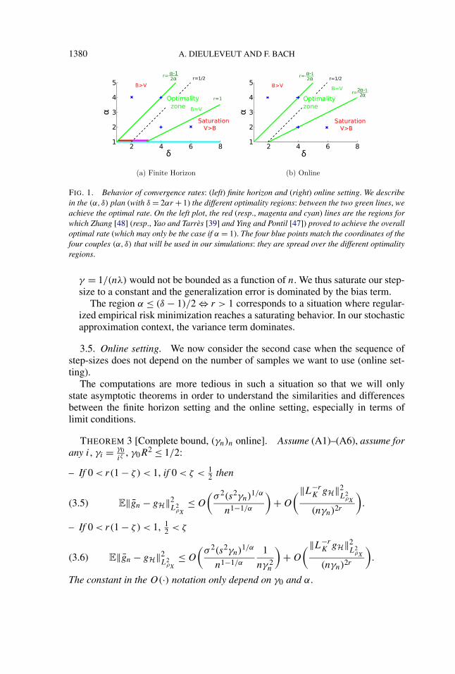
2αr+1 is increasing in both parameters.– Different regions: in Figure 1(a), we plot in the plan of coordinates α, δ (with
δ = 2αr + 1) our limit conditions concerning our assumptions, that is, r = 1⇔δ = 2α + 1 and α−1
2α= r ⇔ α = δ. The region between the two green lines is
the region for which the optimal rate of estimation is reached. The dashed linesstands for r = 1/2, which has appeared to be meaningless in our context.
The region α ≥ δ⇔ α−12α
> r corresponds to a situation where regularizedempirical risk minimization would still be optimal, but with a regularizationparameter λ that decays faster than 1/n, and thus, our corresponding step-size
1380 A. DIEULEVEUT AND F. BACH
FIG. 1. Behavior of convergence rates: (left) finite horizon and (right) online setting. We describein the (α, δ) plan (with δ = 2αr + 1) the different optimality regions: between the two green lines, weachieve the optimal rate. On the left plot, the red (resp., magenta and cyan) lines are the regions forwhich Zhang [48] (resp., Yao and Tarrès [39] and Ying and Pontil [47]) proved to achieve the overalloptimal rate (which may only be the case if α = 1). The four blue points match the coordinates of thefour couples (α, δ) that will be used in our simulations: they are spread over the different optimalityregions.
γ = 1/(nλ) would not be bounded as a function of n. We thus saturate our step-size to a constant and the generalization error is dominated by the bias term.
The region α ≤ (δ − 1)/2⇔ r > 1 corresponds to a situation where regular-ized empirical risk minimization reaches a saturating behavior. In our stochasticapproximation context, the variance term dominates.
3.5. Online setting. We now consider the second case when the sequence ofstep-sizes does not depend on the number of samples we want to use (online set-ting).
The computations are more tedious in such a situation so that we will onlystate asymptotic theorems in order to understand the similarities and differencesbetween the finite horizon setting and the online setting, especially in terms oflimit conditions.
THEOREM 3 [Complete bound, (γn)n online]. Assume (A1)–(A6), assume forany i, γi = γ0
iζ, γ0R
2 ≤ 1/2:
– If 0 < r(1− ζ ) < 1, if 0 < ζ < 12 then
E‖gn − gH‖2L2
ρX
≤O
(σ 2(s2γn)
1/α
n1−1/α
)+O
(‖L−rK gH‖2
L2ρX
(nγn)2r
).(3.5)
– If 0 < r(1− ζ ) < 1, 12 < ζ
E‖gn − gH‖2L2
ρX
≤O
(σ 2(s2γn)
1/α
n1−1/α
1
nγ 2n
)+O
(‖L−rK gH‖2
L2ρX
(nγn)2r
).(3.6)
The constant in the O(·) notation only depend on γ0 and α.

NONPARAMETRIC STOCHASTIC APPROXIMATION 1381
Theorem 3 is proved in Appendix II.4 in [15]. In the first case, the main bias andvariance terms are the same as in the finite horizon setting, and so is the optimalchoice of ζ . However, in the second case, the variance term behavior changes: itdoes not decrease any more when ζ increases beyond 1/2. Indeed, in such a caseour constant averaging procedure puts to much weight on the first iterates, thuswe do not improve the variance bound by making the learning rate decrease faster.Other types of averaging, as proposed, for example, in [25], could help to improvethe bound.
Moreover, this extra condition thus changes a bit the regions where we get theoptimal rate [see Figure 1(b)], and we have the following corollary.
COROLLARY 3 (Optimal decreasing γn). Assume (A1)–(A6) [in this corol-lary, O(·) stands for a constant depending on α,‖L−r
K gH‖L2ρX
, s, σ 2, γ0 and uni-
versal constants]:
1. If α−12α
< r < 2α−12α
, with γn = γ0n(−2αr−1+α)/(2αr+1) for any n ≥ 1 we get
the rate
E‖gn − gH‖2L2
ρX
=O(n−2αr/(2αr+1)).(3.7)
2. If 2α−12α
< r , with γn = γ0n−1/2 for any n≥ 1, we get the rate
E‖gn − gH‖2L2
ρX
=O(n−(2α−1)/(2α)).(3.8)
3. If 0 < r < α−12α
, with γn = γ0 for any n ≥ 1, we get the rate given in (3.4).Indeed the choice of a constant learning rate naturally results in an online proce-dure.
This corollary is directly derived from Theorem 3, balancing the two mainterms. The only difference with the finite horizon setting is the shrinkage of theoptimality region as the condition r < 1 is replaced by r < 2α−1
2α< 1 [see Fig-
ure 1(b)]. In the next section, we relate our results to existing work.
4. Links with existing results. In this section, we relate our results from theprevious section to existing results.
4.1. Euclidean spaces. Recently, Bach and Moulines showed in [5] that forleast squares regression, averaged stochastic gradient descent achieved a rate ofO(1/n), in a finite-dimensional Hilbert space (Euclidean space), under the sameassumptions as above (except the first one of course), which is replaced by:
(A1-f) H is a d-dimensional Euclidean space.
They showed the following result.

1382 A. DIEULEVEUT AND F. BACH
PROPOSITION 5 (Finite-dimensions [5]). Assume (A1-f), (A2)–(A6). Then forγ = 1
4R2 ,
E[ε(gn)− ε(gH)
]≤ 4
n
[σ√
d +R‖gH‖H]2.(4.1)
We show that we can deduce such a result from Theorem 2 (and even withcomparable constants). Indeed under (A1-f) we have:
– If E[‖xn‖2] ≤R2 then � � R2I and (A3) is true for any α ≥ 1 with s2 =R2dα .Indeed λi ≤ R2 if i ≤ d and λi = 0 if i > d + 1 so that for any α > 1, i ∈ N∗,λi ≤R2 dα
iα.
– As we are in a finite-dimensional space (A4) is true for r = 1/2 as ‖T −1/2×gH‖2
L2ρX
= ‖gH‖2H.
Under such remarks, the following corollary may be deduced from Theorem 2.
COROLLARY 4. Assume (A1-f), (A2)–(A6), then for any α > 1, with γR2 ≤1/4,
E‖gn − gH‖2L2
ρX
≤ 4σ 2
n
(1+ (
R2γ dαn)1/α)+ 4
‖gH‖2H
nγ
so that, when α→∞,
E[ε(gn)− ε(gH)
]≤ 4
n
(σ√
d +R‖gH‖H 1√γR2
)2
.
This bound is easily comparable to (4.1) and shows that our more general analy-sis has not lost too much. Moreover, our learning rate is proportional to n−1/(2α+1)
with r = 1/2, so tends to behave like a constant when α→∞, which recovers theconstant step set-up from [5].
Moreover, N. Flammarion proved (personnal communication, 05/2014), usingthe same type of techniques that their bound could be extended to
E[ε(gn)− ε(gH)
]≤ 8σ 2d
n+ 4R4(1+ γ dR2)
‖�−1/2gH‖2
(γR2)2n2 ,(4.2)
a result that may be deduced of the following more general corollaries of our The-orem 2.
COROLLARY 5. Assume (A1-f), (A2)–(A6), and, for some q ∈ [−1/2;1/2],‖�−qgH‖2
H = ‖�−(q+1/2)gH‖2L2
ρX
<∞, then
E[ε(gn)− ε(gH)
]≤ 16
σ 2 tr(�1/α)(γ n)1/α
n+ 8
R4(q+1/2)(1+ τn,γ,q+1/2,α)‖�−qgH‖2H
(nγR2)2(q+1/2).

NONPARAMETRIC STOCHASTIC APPROXIMATION 1383
Such a result is derived from Theorem 2 and with the stronger assumptiontr(�1/α) <∞ clearly satisfied in finite dimension, and with r = q + 1/2. Notethat the result above is true for all values of α ≥ 1 and all q ∈ [−1/2;1/2] (forthe ones with infinite ‖�−(q+1/2)gH‖2
L2ρX
, the statement is trivial). This shows that
we may take the infimum over all possible α ≤ 1 and q ∈ [−1/2;1/2], showingadaptivity of the estimator to the spectral decay of � and the smoothness of theoptimal prediction function gH.
The residual term τn,γ,q+ 1
2 ,αis the same as in Theorem 2. When α→∞, it
goes to a term which scales like (γ d)2q , if q ∈ [0;1/2] (it is 0 otherwise).Thus, with α→∞, we obtain the following.
COROLLARY 6. Assume (A1-f), (A2)–(A6) and for some q ∈ [−1/2;1/2],‖�−qgH‖2
H = ‖�−(q+1/2)gH‖2L2
ρX
<∞, then
E[ε(gn)− ε(gH)
]≤ 16σ 2d
n+ 8R4(q+1/2)(1+ (γR2d)2q∨0) ‖�−qgH‖2
H(nγR2)2(q+1/2)
.
– This final result bridges the gap between Proposition 5 (q = 0), and its extension(4.2) (q = 1/2). The constants 16 and 8 come from the upper bounds (a+b)2 ≤a2 + b2 and 1+ 1/
√d ≤ 2 and are thus nonoptimal.
– Moreover, we can also derive from Corollary 5, with α = 1, q = 0, and γ ∝n−1/2, we recover the rate O(n−1/2) (where the constant does not depend on thedimension d of the Euclidean space). Such a rate was described, for example,in [29].
Note that linking our work to the finite-dimensional setting is made using thefact that our assumption (A3) is true for any α > 1.
4.2. Optimal rates of estimation. In some situations, our stochastic approxi-mation framework leads to “optimal” rates of prediction in the following sense.In [10], Theorem 2, a minimax lower bound was given: let P(α, r) (α > 1, r ∈[1/2,1]) be the set of all probability measures ρ on X ×Y , such that:
– |y| ≤Mρ almost surely,– T −rgρ ∈ L2
ρX,
– the eigenvalues (μj )j∈N arranged in a nonincreasing order, are subject to thedecay μj =O(j−α).
Then the following minimax lower rate stands:
lim infn→∞ inf
gnsup
ρ∈P(b,r)
P{ε(gn)− ε(gρ) > Cn−2rα/(2rα+1)}= 1,
for some constant C > 0 where the infimum in the middle is taken over all algo-rithms that are maps ((xi, yi)1≤i≤n) �→ gn ∈H.

1384 A. DIEULEVEUT AND F. BACH
When making assumptions (a3)–(a4), the assumptions regarding the predictionproblem (i.e., the optimal function gρ) are summarized in the decay of the com-ponents of gρ in an orthonormal basis, characterized by the constant δ. Here, theminimax rate of estimation (see, e.g., [21]) is O(n−1+1/δ) which is the same asO(n−2rα/(2rα+1)) with the identification δ = 2αr + 1.
That means the rate we get is optimal for α−12α
< r < 1 in the finite horizonsetting, and for α−1
2α< r < 2α−1
2αin the online setting. This is the region between
the two green lines on Figure 1.
4.3. Regularized stochastic approximation. It is interesting to link our resultsto what has been done in [45] and [39] in the case of regularized least-mean-squares, so that the recursion is written
gn = gn−1 − γn
((gn−1(xn)− yn
)Kxn + λngn−1
)with (gn−1(xn)− yn)Kxn + λngn−1 an unbiased gradient of 1
2Eρ[(g(x)− y)2] +λn
2 ‖g‖2. In [39], the following result is proved (Remark 2.8 following Theorem C).
THEOREM 4 (Regularized, nonaveraged stochastic gradient [39]). Assumethat T −rgρ ∈ L2
ρXfor some r ∈ [1/2,1]. Assume the kernel is bounded and Y
compact. Then with probability at least 1− κ , for all t ∈N,
ε(gn)− ε(gρ)≤Oκ
(n−2r/(2r+1)),
where Oκ stands for a constant which depends on κ .
No assumption is made on the covariance operator beyond being trace class, butonly on ‖T −rgρ‖L2
ρX[thus no assumption (A3)]. A few remarks may be made:
1. They get almost-sure convergence, when we only get convergence in expecta-tion. We could perhaps derive a.s. convergence by considering moment boundsin order to be able to derive convergence in high probability and to use Borel–Cantelli lemma.
2. They only assume 12 ≤ r ≤ 1, which means that they assume the regression
function to lie in the RKHS.
4.4. Unregularized stochastic approximation. In [47], Ying and Pontil stud-ied the same unregularized problem as we consider, under assumption (A4). Theyobtain the same rates as above [n−2r/(2r+1) log(n)] in both online case (with0≤ r ≤ 1
2 ) and finite horizon setting (0 < r).They led as an open problem to improve bounds with some additional informa-
tion on some decay of the eigenvalues of T , a question which is answered here.Moreover, Zhang [48] also studies stochastic gradient descent algorithms in
an unregularized setting, also with averaging. As described in [47], his result
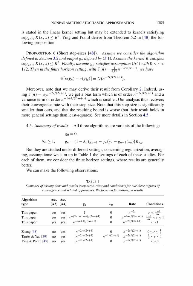
NONPARAMETRIC STOCHASTIC APPROXIMATION 1385
is stated in the linear kernel setting but may be extended to kernels satisfyingsupx∈X K(x,x) ≤ R2. Ying and Pontil derive from Theorem 5.2 in [48] the fol-lowing proposition.
PROPOSITION 6 (Short step-sizes [48]). Assume we consider the algorithmdefined in Section 3.2 and output gn defined by (3.1). Assume the kernel K satisfiessupx∈X K(x,x)≤ R2. Finally, assume gρ satisfies assumption (A4) with 0 < r <
1/2. Then in the finite horizon setting, with �(n)= 14R2 n
−2r/(2r+1), we have
E[ε(gn)− ε(gH)
]=O(n−2r/(2r+1)).
Moreover, note that we may derive their result from Corollary 2. Indeed, us-ing �(n)= γ0n
−2r/(2r+1), we get a bias term which is of order n−2r/(2r+1) and avariance term of order n−1+1/(2rα+α) which is smaller. Our analysis thus recoverstheir convergence rate with their step-size. Note that this step-size is significantlysmaller than ours, and that the resulting bound is worse (but their result holds inmore general settings than least-squares). See more details in Section 4.5.
4.5. Summary of results. All three algorithms are variants of the following:
g0 = 0,
∀n≥ 1, gn = (1− λn)gn−1 − γn
(yn − gn−1(xn)
)Kxn.
But they are studied under different settings, concerning regularization, averag-ing, assumptions: we sum up in Table 1 the settings of each of these studies. Foreach of them, we consider the finite horizon settings, where results are generallybetter.
We can make the following observations.
TABLE 1Summary of assumptions and results (step-sizes, rates and conditions) for our three regions of
convergence and related approaches. We focus on finite-horizon results
Algorithm Ass. Ass.type (A3) (A4) γn λn Rate Conditions
This paper yes yes 1 0 n−2r r < α−12α
This paper yes yes n−(2αr+1−α)/(2αr+1) 0 n−2αr/(2αr+1) α−12α
< r < 1This paper yes yes n−(α+1)/(2α+1) 0 n−2α/(2α+1) r > 1
Zhang [48] no yes n−2r/(2r+1) 0 n−2r/(2r+1) 0≤ r ≤ 12
Tarrès & Yao [39] no yes n−2r/(2r+1) n−1/(2r+1) n−2r/(2r+1) 12 ≤ r ≤ 1
Ying & Pontil [47] no yes n−2r/(2r+1) 0 n−2r/(2r+1) r > 0

1386 A. DIEULEVEUT AND F. BACH
– Dependence of the convergence rate on α: For learning with any kernel withα > 1, we strictly improve the asymptotic rate compared to related methods thatonly assume summability of eigenvalues: indeed, the function x �→ x/(x+ 1) isincreasing on R+. If we consider a given optimal prediction function and a givenkernel with which we are going to learn the function, considering the decrease ineigenvalues allows to adapt the step-size and obtain an improved learning rate.Namely, we improved the previous rate −2r
2r+1 up to −2αr2αr+1 .
– Worst-case result in r : In the setting of assumptions (a3), (a4), given δ, theoptimal rate of convergence is known to be O(n−1+1/δ), where δ = 2αr+1. Wethus get the optimal rate, as soon as α < δ < 2α+ 1, while the other algorithmsget the sub-optimal rate n(δ−1)/(δ+α−1) under various conditions. Note that thissub-optimal rate becomes close to the optimal rate when α is close to one, thatis, in the worst-case situation. Thus, in the worst case (α arbitrarily close toone), all methods behave similarly, but for any particular instance where α > 1,our rates are better.
– Choice of kernel: In the setting of assumptions (a3), (a4), given δ, in order to getthe optimal rate, we may choose the kernel (i.e., α) such that α < δ < 2α + 1(i.e., neither too big, nor too small), while other methods need to choose a kernelfor which α is as close to one as possible, which may not be possible in practice.
– Improved bounds: Ying and Pontil [47] only give asymptotic bounds, while wehave exact constants for the finite horizon case. Moreover, there are some loga-rithmic terms in [47] which disappear in our analysis.
– Saturation: Our method does saturate for r > 1, while the nonaveraged frame-work of [47] does not (but does not depend on the value of α). We conjecturethat a proper nonuniform averaging scheme (that puts more weight on the latestiterates), we should get the best of both worlds.
5. Experiments on artificial data. Following [47], we consider synthetic ex-amples with smoothing splines on the circle, where our assumptions (A3)–(A4)are easily satisfied.
5.1. Splines on the circle. The simplest example to match our assumptionsmay be found in [43]. We consider Y = gρ(X)+ ε, with X ∼ U[0;1] is a uniformrandom variable in [0,1], and gρ in a particular RKHS (which is actually a Sobolevspace).
Let H be the collection of all zero-mean periodic functions on [0;1] of the form
f : t �→√2∞∑i=1
ai(f ) cos(2πit)+√2∞∑i=1
bi(f ) sin(2πit),
with
‖f ‖2H =
∞∑i=1
(ai(f )2 + bi(f )2)
(2πi)2m <∞.

NONPARAMETRIC STOCHASTIC APPROXIMATION 1387
This means that the mth derivative of f , f (m) is in L2([0;1]). We consider theinner product
〈f,g〉H =∞∑i=1
(2πi)2m(ai(f )ai(g)+ bi(f )bi(g)
).
It is known that H is an RKHS and that the reproducing kernel Rm(s, t) for H is
Rm(s, t)=∞∑i=1
2
(2πi)2m
[cos(2πis) cos(2πit)+ sin(2πis) sin(2πit)
]
=∞∑i=1
2
(2πi)2mcos
(2πi(s − t)
).
Moreover, the study of Bernoulli polynomials gives a close formula for R(s, t),that is,
Rm(s, t)= (−1)m−1
(2m)! B2m
({s − t}),with Bm denoting the mth Bernoulli polynomial and {s − t} the fractional part ofs − t [43].
We can derive the following proposition for the covariance operator whichmeans that our assumption (A3) is satisfied for our algorithm in H when X ∼U[0;1], with α = 2m, and s = 2(1/2π)m.
PROPOSITION 7 (Covariance operator for smoothing splines). If X ∼ U[0;1],then in H:
1. The eigenvalues of � are all of multiplicity 2 and are λi = (2πi)−2m.2. The eigenfunctions are φc
i : t �→√
2 cos(2πit) and φsi : t �→
√2 sin(2πit).
PROOF. For φci , we have (a similar argument holds for φs
i )
T(φc
i
)(s)=
∫ 1
0R(s, t)
√2 cos(2πit) dt
=(∫ 1
0
2
(2iπ)2m
√2 cos(2πit)2 dt
)cos(2πis)= λi
√2 cos(2πis)
= λiφci (s).
It is well known that (φci , φ
si )i≥0 is an orthonormal system (the Fourier ba-
sis) of the functions in L2([0;1]) with zero mean, and it is easy to check that((2iπ)−mφc
i , (2iπ)−mφsi )i≥1 is an orthonormal basis of our RKHS H (this may
also be seen as a consequence of the fact that T 1/2 is an isometry). �
1388 A. DIEULEVEUT AND F. BACH
Finally, considering gρ(x) = Bδ/2(x) with δ = 2αr + 1 ∈ 2N, our assumption(A4) holds. Indeed it implies (a3)–(a4), with α > 1, δ = 2αr + 1, since for anyk ∈N, Bk(x)=−2k!∑∞i=1
cos(2iπx−kπ/2)
(2iπ)k(see, e.g., [1]).
We may notice a few points:
1. Here the eigenvectors do not depend on the kernel choice, only the re-normalisation constant depends on the choice of the kernel. Especially theeigenbasis of T in L2
ρXdoes not depend on m. That can be linked with the
previous remarks made in Section 4.2. Assumption (A3) defines here the size of the RKHS: the smaller α = 2m is, the
bigger the space is, the harder it is to learn a function.
In the next section, we illustrate on such a toy model our main results and com-pare our learning algorithm to Ying and Pontil’s [47], Tarrès and Yao’s [39] andZhang’s [48] algorithms.
5.2. Experimental set-up. We use gρ(x) = Bδ/2(x) with δ = 2αr + 1, asproposed above, with B1(x) = x − 1
2 , B2(x) = x2 − x + 16 and B3(x) = x3 −
32x2 + 1
2x.We give in Table 2 the functions used for simulations in a few cases that span
our three regions. We also remind the choice of γ proposed for the 4 algorithms.We always use the finite horizon setting.
5.3. Optimal learning rate for our algorithm. In this section, we empiricallysearch for the best choice of a finite horizon learning rate, in order to check ifit matches our prediction. For a certain number of values for n, distributed ex-ponentially between 1 and 103.5, we look for the best choice �best(n) of a con-stant learning rate for our algorithm up to horizon n. In order to do that, fora large number of constants C1, . . . ,Cp , we estimate the expectation of errorE[ε(gn(γ = Ci)) − ε(gρ)] by averaging over 30 independent samples of size n,then report the constant giving minimal error as a function of n in Figure 2.We consider here the situation α = 2, r = 0.75. We plot results in a logarithmicscale in Figure 2, and evaluate the asymptotic decrease of �best(n) by fitting anaffine approximation to the second half of the curve. We get a slope of −0.51,which matches our choice of −0.5 from Corollary 2. Although, our theoretical re-sults are only upper-bounds, we conjecture that our proof technique also leads tolower-bounds in situations where assumptions (a3)–(a4) hold (like in this experi-ment).
5.4. Comparison to competing algorithms. In this section, we compare theconvergence rates of the four algorithms described in Section 4.5. We considerthe different choices of (r, α) as described in Table 2 in order to go all over the

NONPARAMETRIC STOCHASTIC APPROXIMATION 1389
FIG. 2. Optimal learning rate �best(n) for our algorithm in the finite horizon setting (plain ma-genta). The dashed green curve is a first order affine approximation of the second half of the magentacurve.
different optimality situations. The main properties of each algorithm are describedin Table 1. However we may note:
– For our algorithm, �(n) is chosen accordingly to Corollary 2, with γ0 = 1R2 .
– For Ying and Pontil’s algorithm, accordingly to Theorem 6 in [47], we con-sider �(n)= γ0n
−2r/(2r+1). We choose γ0 = 1R2 which behaves better than the
proposed r64(1+R4)(2r+1)
.
– For Tarrès and Yao’s algorithm, we refer to Theorem C in [39], and consider�(n) = a(n0 + n)−2r/(2r+1) and �(n) = 1
a(n0 + n)−1/(2r+1). The theorem is
stated for all a ≥ 4: we choose a = 4.– For Zhang’s algorithm, we refer to Part 2.2 in [47], and choose �(n) =
γ0n−2r/(2r+1) with γ0 = 1
R2 which behaves better than the proposed choice1
4(1+R2).
In Figure 3, we plot the expected error as a function of the number of points.Finally, we sum up the rates that were both predicted and derived for the four
algorithms in the four cases for (α, δ) in Table 3. It appears that (a) we approxima-tively match the predicted rates in most cases (they would if n was larger), (b) ourrates improve on existing work.
TABLE 2Different choices of the parameters α, r and the corresponding convergence rates and step-sizes.The (α, δ) coordinates of the four choices of couple “(kernel, objective function)” are mapped on
Figure 1. They are spread over the different optimality regions
r α δ K gρlog(γ )log(n)
(this paper) log(γ )log(n)
(previous)
0.75 2 4 R1 B2 −1/2=−0.5 −3/5=−0.60.375 4 4 R2 B2 0 −3/7�−0.431.25 2 6 R1 B3 −3/7�−0.43 −5/7�−0.710.125 4 2 R2 B1 0 −1/5=−0.2
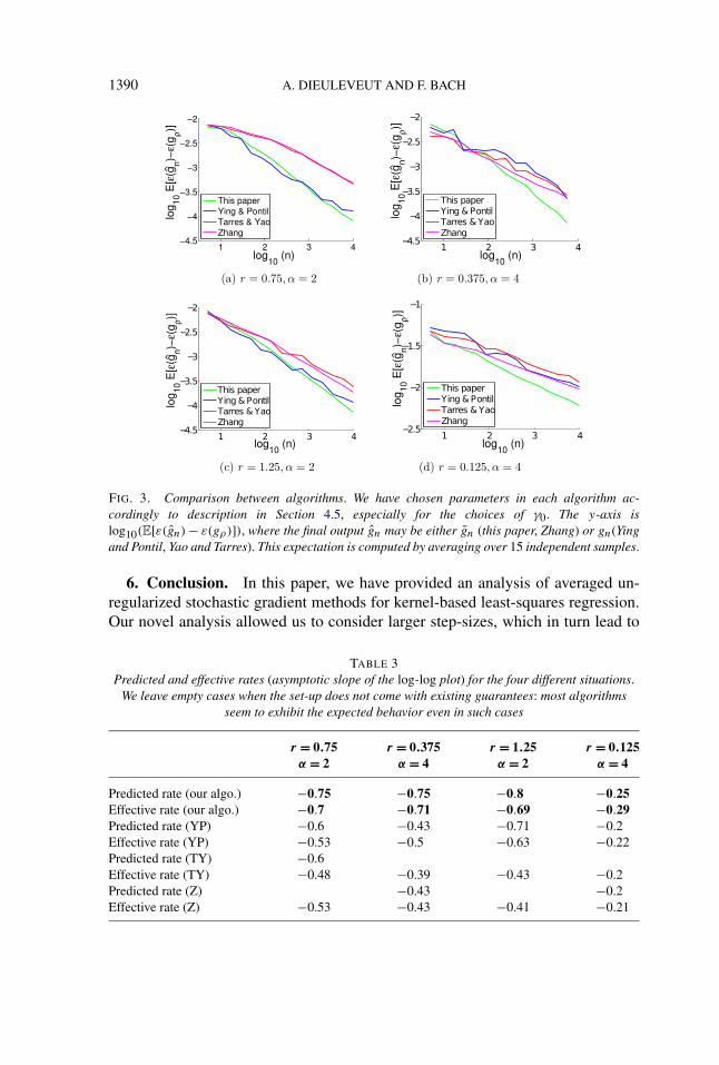
1390 A. DIEULEVEUT AND F. BACH
FIG. 3. Comparison between algorithms. We have chosen parameters in each algorithm ac-cordingly to description in Section 4.5, especially for the choices of γ0. The y-axis islog10(E[ε(gn)− ε(gρ)]), where the final output gn may be either gn (this paper, Zhang) or gn(Yingand Pontil, Yao and Tarres). This expectation is computed by averaging over 15 independent samples.
6. Conclusion. In this paper, we have provided an analysis of averaged un-regularized stochastic gradient methods for kernel-based least-squares regression.Our novel analysis allowed us to consider larger step-sizes, which in turn lead to
TABLE 3Predicted and effective rates (asymptotic slope of the log-log plot) for the four different situations.
We leave empty cases when the set-up does not come with existing guarantees: most algorithmsseem to exhibit the expected behavior even in such cases
r = 0.75 r = 0.375 r = 1.25 r = 0.125α = 2 α = 4 α = 2 α = 4
Predicted rate (our algo.) −0.75 −0.75 −0.8 −0.25Effective rate (our algo.) −0.7 −0.71 −0.69 −0.29Predicted rate (YP) −0.6 −0.43 −0.71 −0.2Effective rate (YP) −0.53 −0.5 −0.63 −0.22Predicted rate (TY) −0.6Effective rate (TY) −0.48 −0.39 −0.43 −0.2Predicted rate (Z) −0.43 −0.2Effective rate (Z) −0.53 −0.43 −0.41 −0.21

NONPARAMETRIC STOCHASTIC APPROXIMATION 1391
optimal estimation rates for many settings of eigenvalue decay of the covarianceoperators and smoothness of the optimal prediction function. Moreover, we haveworked on a more general setting than previous work that includes most interestingcases of positive definite kernels.
Our work can be extended in a number of interesting ways: First, (a) wehave considered results in expectation; following the higher-order moment boundsfrom [5] in the Euclidean case, we could consider higher-order moments, whichin turn could lead to high-probability results or almost-sure convergence. More-over, (b) while we obtain optimal convergence rates for a particular regime of ker-nels/objective functions, using different types of averaging (i.e., nonuniform) maylead to optimal rates in other regimes. Besides, (c) following [5], we could extendour results for infinite-dimensional least-squares regression to other smooth lossfunctions, such as for logistic regression, where an online Newton algorithm withthe same running-time complexity would also lead to optimal convergence rates.Also, (d) the running-time complexity of our stochastic approximation proceduresis still quadratic in the number of samples n, which is unsatisfactory when n islarge; by considering reduced set-methods [3, 8, 13], we hope to able to obtaina complexity of O(dnn), where dn is such that the convergence rate is O(dn/n),which would extend the Euclidean space result, where dn is constant equal to thedimension. Finally, (e) in order to obtain the optimal rates when the bias term dom-inates our generalization bounds, it would be interesting to combine our spectralanalysis with recent accelerated versions of stochastic gradient descent which havebeen analyzed in the finite-dimensional setting [17].
APPENDIX A: MINIMAL ASSUMPTIONS
A.1. Definitions. We first define the set of square ρX-integrable func-tions L2
ρX:
L2ρX=
{f :X →R
/∫X
f 2(t) dρX(t) <∞};
we will always make the assumptions that this space is separable (this is the casein most interesting situations. See [40] for more details.) L2
ρXis its quotient under
the equivalence relation given by
f ≡ g ⇔∫X
(f (t)− g(t)
)2dρX(t)= 0,
which makes it a separable Hilbert space (see, e.g., [24]).We denote p the canonical projection from L2
ρXinto L2
ρXsuch that p : f �→ f ,
with f = {g ∈ L2ρX
, s.t. f ≡ g}.Under assumptions (A1), (A2) or (A1′), (A2′), any function in H in L2
ρX. More-
over, under (A1), (A2) the spaces H and p(H) may be identified, where p(H) is
the image of H via the mapping p ◦ i :H i−→L2ρX
p−→L2ρX
, where i is the trivialinjection from H into L2
ρX.

1392 A. DIEULEVEUT AND F. BACH
A.2. Isomorphism. As it has been explained in the main text, the minimiza-tion problem will appear to be an approximation problem in L2
ρX, for which we
will build estimates in H. However, to derive theoretical results, it is easier to con-sider it as an approximation problem in the Hilbert space L2
ρX, building estimates
in p(H).We thus need to define a notion of the best estimation in p(H). We first define
the closure F (with respect to ‖ · ‖L2ρX
) of any set F ⊂ L2ρX
as the set of limits of
sequences in F . The space p(H) is a closed and convex subset in L2ρX
. We can
thus define gH = arg minf∈p(H) ε(g), as the orthogonal projection of gρ on p(H),using the existence of the projection on any closed convex set in a Hilbert space.See Proposition 8 in Appendix A in [15] for details.
PROPOSITION 8 (Definition of best approximation function). Assume (A1)–(A2). The minimum of ε(f ) in p(H) is attained at a certain gH (which is uniqueand well defined in L2
ρX).
Where p(H)= {f ∈ L2ρX\∃(fn)⊂ p(H),‖fn−f ‖L2
ρX→ 0} is the set of func-
tions f for which we can hope for consistency, that is, having a sequence (fn)n ofestimators in H such that ε(fn)→ ε(f ).
The properties of our estimator, especially its rate of convergence will stronglydepend on some properties of both the kernel, the objective function and the dis-tributions, which may be seen through the properties of the covariance opera-tor which is defined in the main text. We have defined the covariance operator,� : H→ H. In the following, we extend such an operator as an endomorphismT from L2
ρXto L2
ρXand by projection as an endomorphism T = p ◦ T from L2
ρX
to L2ρX
. Note that T is well defined as∫X g(t)Kt dρX (t) does not depend on the
function g chosen in the class of equivalence of g.
DEFINITION 3 (Extended covariance operator). Assume (A1)–(A2). We de-fine the operator T as follows (this expectation is formally defined as a Bochnerexpectation in H):
T L2ρX→ L2
ρX,
g �→∫X
g(t)Kt dρX (t),
so that for any z ∈X , T (g)(z)= ∫X g(x)K(x, z) dρX (t)= E[g(X)K(X, z)].
A first important remark is that �f = 0 implies 〈f,�f 〉 = ‖f ‖2L2
ρX
= 0,
that is p(Ker(�)) = {0}. However, � may not be injective (unless ‖f ‖2L2
ρX
⇒f = 0, which is true when f is continuous and ρX has full support). � and T mayindependently be injective or not.

NONPARAMETRIC STOCHASTIC APPROXIMATION 1393
The operator T (which is an endomorphism of the separable Hilbert space L2ρX
)can be reduced in some Hilbertian eigenbasis of L2
ρX. The linear operator T hap-
pens to have an image included in H, and the eigenbasis of T in L2ρX
may alsobe seen as eigenbasis of � in H (see the proof in Appendix I.2, Proposition 18in [15]).
PROPOSITION 9 (Decomposition of �). Assume (A1)–(A2). The image of Tis included in H: Im(T ) ⊂H, that is, for any f ∈ L2
ρX, T f ∈H. Moreover, for
any i ∈ I , φHi = 1
μiT φi ∈ H ⊂ L2
ρXis a representant for the equivalence class
φi , that is, p(φHi ) = φi . Moreover μ
1/2i φH
i is an orthonormal eigensystem of theorthogonal supplement S of the null space Ker(�). That is:
– ∀i ∈ I,�φHi = μiφ
Hi .
– H=Ker(�)⊥⊕S .
Such decompositions allow to define T r : L2ρX→H for r ≥ 1/2. Indeed, com-
pleteness allows to define infinite sums which satisfy a Cauchy criterion. See proofin Appendix I.2, Proposition 19 in [15]. Note the different condition concerning r
in the definitions. For r ≥ 1/2, T r = p ◦ T r . We need r ≥ 1/2, because (μ1/2i φH )
is an orthonormal system of S .
DEFINITION 4 (Powers of T ). We define, for any r ≥ 1/2, T r : L2ρX→H, for
any h ∈Ker(T ) and (ai)i∈I such that∑
i∈I a2i <∞, through
T r
(h+∑
i∈Iaiφi
)=∑
i∈Iaiμ
ri φ
Hi .
We have two decompositions of L2ρX=Ker(T )
⊥⊕ S and H=Ker(�)⊥⊕S . The
two orthogonal supplements S and S happen to be related through the mappingT 1/2, as stated in Proposition 4: T 1/2 is an isomorphism from S into S . It alsohas he following consequences, which generalizes Corollary 1.
COROLLARY 7.
– T 1/2(S) = p(H), that is, any element of p(H) may be expressed as T 1/2g forsome g ∈ L2
ρX.
– For any r ≥ 1/2, T r(S)⊂H, because T r(S)⊂ T 1/2(S), that is, with large pow-ers r , the image of T r is in the projection of the Hilbert space.
– ∀r > 0, T r(L2ρX
) = S = T 1/2(L2ρX
) = H, because (a) T 1/2(L2ρX
) = p(H) and
(b) for any r > 0, T r(L2ρX
) = S. In other words, elements of p(H) (on which
our minimization problem attains its minimum), may seen as limits (in L2ρX
) of
elements of T r(L2ρX
), for any r > 0.
1394 A. DIEULEVEUT AND F. BACH
– p(H) is dense in L2ρX
if and only if T is injective.
A.3. Mercer theorem generalized. Finally, although we will not use it in therest of the paper, we can state a version of Mercer’s theorem, which does not makeany more assumptions that are required for defining RKHSs.
PROPOSITION 10 (Kernel decomposition). Assume (A1)–(A2). We have forall x, y ∈X ,
K(x,y)=∑i∈I
μiφHi (x)φH
i (y)+ g(x, y),
and we have for all x ∈ X ,∫X g(x, y)2 dρX(y)= 0. Moreover, the convergence of
the series is absolute.
We thus obtain a version of Mercer’s theorem (see Appendix I.5.3 in [15]) with-out any topological assumptions. Moreover, note that (a) S is also an RKHS,with kernel (x, y) �→∑
i∈I μiφHi (x)φH
i (y) and (b) that given the decompositionabove, the optimization problem in S and H have equivalent solutions. More-over, considering the algorithm below, the estimators we consider will almostsurely build equivalent functions (see Appendix I.4 in [15]). Thus, we could as-sume without loss of generality that the kernel K is exactly equal to its expansion∑
i∈I μiφHi (x)φH
i (y).
A.4. Complementary (A6) assumption. Under minimal assumptions, wealso have to make a complementary moment assumption:
(A6′) There exists R > 0 and σ > 0 such that E[�⊗�]� σ 2�, and E(K(X,X)×KX ⊗KX) � R2� where � denotes the order between self-adjoint opera-tors.
In other words, for any f ∈H, we have: E[K(X,X)f (X)2] ≤R2E[f (X)2]. Suchan assumption is implied by (A2), that is, if K(X,X) is almost surely bounded byR2: this constant can then be understood as the radius of the set of our data points.However, our analysis holds in these more general set-ups where only fourth-ordermoment of ‖Kx‖H =K(x,x)1/2 is finite.
APPENDIX B: SKETCH OF THE PROOFS
Our main theorems are Theorem 2 and Theorem 3, respectively, in the finitehorizon and in the online setting. Corollaries can be easily derived by optimizingover γ the upper bound given in the theorem.
The complete proof is given in Appendix II in [15]. The proof is nearly thesame for finite horizon and online setting. It relies on a refined analysis of stronglyrelated recursions in the RKHS and on a comparison between iterates of the recur-sions (controlling the deviations).

NONPARAMETRIC STOCHASTIC APPROXIMATION 1395
We first present the sketch of the proof for the finite-horizon setting: We wantto analyze the error of our sequence of estimators (gn) such that g0 = 0 and
gn = gn−1 − γn
[yn − 〈gn−1,Kxn〉H
]Kxn,
gn = (I − γKxn ⊗Kxn)gn−1 + γynKxn,
gn − gH = (I − γ ˜Kxn ⊗Kxn)(gn−1 − gH)+ γ�n.
Where we have denoted �n = (yn − gH(xn))Kxn the residual, which has 0 mean,
and ˜Kxn ⊗Kxn : L2ρX→H an a.s. defined extension of Kxn ⊗Kxn :H→H, such
that ˜Kxn ⊗Kxn(f )= f (xn)Kxn , that will be denoted for simplicity Kxn ⊗Kxn inthis section.
Finally, we are studying a sequence (ηn)n = (gn − gH)n defined by
η0 = gH,
ηn = (I − γnKxn ⊗Kxn)ηn−1 + γn�n.
We first consider splitting this recursion in two simpler recursions ηinitn and ηnoise
n
such that ηn = ηinitn + ηnoise
n :
• (ηinitn )n defined by
ηinit0 = gH and ηinit
n = (I − γKxn ⊗Kxn)ηinitn−1.
ηinitn is the part of (ηn)n which is due to the initial conditions (it is equivalent to
assuming �n ≡ 0).• Respectively, let (ηnoise
n )n be defined by
ηnoise0 = 0 and ηnoise
n = (I − γKxn ⊗Kxn)ηnoisen−1 + γ�n.
ηnoisen is the part of (ηn)n which is due to the noise.
We will bound ‖ηn‖ by ‖ηinitn ‖ + ‖ηnoise
n ‖ using Minkowski’s inequality. That ishow the bias-variance trade-off originally appears.
Next, we notice that E[Kxn ⊗Kxn] = T , and thus define “semi-stochastic” ver-sions of the previous recursions by replacing Kxn ⊗Kxn by its expectation:
For the initial conditions: (η0,initn )n∈N so that
η0,init0 = gH, η0,init
n = (I − γT )η0,initn−1 ,
which is a deterministic sequence.An algebraic calculation gives an estimate of the norm of η0,init
n , and we canalso bound the residual term ηinit
n − η0,initn , then conclude by Minkowski.
For the variance term: We follow the exact same idea, but have to define asequence of “semi-stochastic recursion,” to be able to bound the residual term.
This decomposition is summed up in Table 4.For the online setting, we follow comparable ideas and end in a similar decom-
position.

1396A
.DIE
UL
EV
EU
TA
ND
F.BA
CH
TABLE 4Error decomposition in the finite horizon setting. All the references refer to lemmas given in Appendix II in [15]
Complete recursion ηn
↙ ↘variance term ηnoise
n | bias term ηinitn
↓ | ↓multiple recursion | semi stochastic variant
↙ ↘ | ↙ ↘main terms ηr
n, r ≥ 1 residual term ηnoisen −∑
ηrn | main term η0
n residual term ηinitn − η0
n
satisfying semi-sto recursions satisf. stochastic recursion | satisf. semi-sto recursion satisf. stochastic recursion↓ Lemma 8 ↓ Lemma 9 | ↓ ↓ Lemma 9
≤ C Variance term →r→∞ 0 | ≤ Bias term residual negligible term
Lemma 5↘ ↙ Lemma 4Theorem 2

NONPARAMETRIC STOCHASTIC APPROXIMATION 1397
Acknowledgement. We thank Nicolas Flammarion for helpful discussions.
REFERENCES
[1] ABRAMOWITZ, M. and STEGUN, I. (1964). Handbook of Mathematical Functions. Dover,New York.
[2] ARONSZAJN, N. (1950). Theory of reproducing kernels. Trans. Amer. Math. Soc. 68 337–404.MR0051437
[3] BACH, F. (2013). Sharp analysis of low-rank kernel matrix approximations. In Proceedings ofthe International Conference on Learning Theory (COLT).
[4] BACH, F. and MOULINES, E. (2011). Non-asymptotic analysis of stochastic approximationalgorithms for machine learning. In Adv. NIPS. Curran Associates, Inc., Granada, Spain.
[5] BACH, F. and MOULINES, E. (2013). Non-strongly-convex smooth stochastic approximationwith convergence rate O(1/n). In Advances in Neural Information Processing Systems(NIPS). Curran Associates, Inc., Lake Tahoe, CA.
[6] BERLINET, A. and THOMAS-AGNAN, C. (2004). Reproducing Kernel Hilbert Spaces in Prob-ability and Statistics. Kluwer Academic, Boston, MA. MR2239907
[7] BLANCHARD, G. and KRÄMER, N. (2010). Optimal learning rates for kernel conjugate gradi-ent regression. In Advances in Neural Inf. Proc. Systems (NIPS) 226–234. Curran Asso-ciates, Inc., Vancouver, Canada.
[8] BORDES, A., ERTEKIN, S., WESTON, J. and BOTTOU, L. (2005). Fast kernel classifiers withonline and active learning. J. Mach. Learn. Res. 6 1579–1619. MR2249866
[9] BREZIS, H. (1983). Analyse Fonctionnelle, Théorie et Applications. Masson, Paris.MR0697382
[10] CAPONNETTO, A. and DE VITO, E. (2007). Optimal rates for the regularized least-squaresalgorithm. Found. Comput. Math. 7 331–368. MR2335249
[11] CUCKER, F. and SMALE, S. (2002). On the mathematical foundations of learning. Bull. Amer.Math. Soc. (N.S.) 39 1–49 (electronic). MR1864085
[12] CUCKER, F. and SMALE, S. (2002). Best choices for regularization parameters in learningtheory: On the bias-variance problem. Found. Comput. Math. 2 413–428. MR1930945
[13] DEKEL, O., SHALEV-SHWARTZ, S. and SINGER, Y. (2005). The Forgetron: A kernel-basedperceptron on a fixed budget. In Adv. NIPS. Curran Associates, Inc., Vancouver, Canada.
[14] DE VITO, E., CAPONNETTO, A. and ROSASCO, L. (2005). Model selection for regularizedleast-squares algorithm in learning theory. Found. Comput. Math. 5 59–85. MR2125691
[15] DIEULEVEUT, A. and BACH, F. (2014). Nonparametric stochastic approximation with largestep sizes. Preprint. Available at arXiv:1408.0361.
[16] ENGL, H. W., HANKE, M. and NEUBAUER, A. (1996). Regularization of Inverse Problems.Mathematics and Its Applications 375. Kluwer Academic, Dordrecht. MR1408680
[17] FLAMMARION, N. and BACH, F. (2015). From averaging to acceleration, there is only a step-size. In Proceedings of the International Conference on Learning Theory (COLT). Micro-tome Publishing, Paris, France.
[18] GOLUB, G. H. and VAN LOAN, C. F. (1996). Matrix Computations, 3rd ed. Johns HopkinsUniv. Press, Baltimore, MD. MR1417720
[19] HAZAN, E. and KALE, S. (2011). Beyond the regret minimization barrier: An optimal algo-rithm for stochastic strongly-convex optimization. In Proceedings of the InternationalConference on Learning Theory (COLT). Microtome Publishing, Budapest, Hungary.
[20] HSU, D., KAKADE, S. M. and ZHANG, T. (2014). Random design analysis of ridge regression.Found. Comput. Math. 14 569–600. MR3201956
[21] JOHNSTONE, I. M. (1994). Minimax Bayes, asymptotic minimax and sparse wavelet priors.In Statistical Decision Theory and Related Topics, V (West Lafayette, IN, 1992) 303–326.Springer, New York. MR1286310

1398 A. DIEULEVEUT AND F. BACH
[22] KIMELDORF, G. and WAHBA, G. (1971). Some results on Tchebycheffian spline functions.J. Math. Anal. Appl. 33 82–95. MR0290013
[23] KIVINEN, J., SMOLA, A. J. and WILLIAMSON, R. C. (2004). Online learning with kernels.IEEE Trans. Signal Process. 52 2165–2176. MR2085578
[24] KOLMOGOROV, A. N. and FOMIN, S. V. (1999). Elements of the Theory of Functions andFunctional Analysis, Vol. 1 Dover, New York.
[25] LACOSTE-JULIEN, S., SCHMIDT, M. and BACH, F. (2012). A simpler approach to obtain-ing an O(1/t) rate for the stochastic projected subgradient method. Preprint. Available atarXiv:1212.2002.
[26] MAHONEY, M. W. (2011). Randomized algorithms for matrices and data. Faund. Trends Mach.Learn. 3 123–224.
[27] MICCHELLI, C. A., XU, Y. and ZHANG, H. (2006). Universal kernels. J. Mach. Learn. Res. 72651–2667. MR2274454
[28] MIKUSINSKI, P. and WEISS, E. (2014). The Bochner integral. Preprint. Available atarXiv:1403.5209.
[29] NEMIROVSKI, A., JUDITSKY, A., LAN, G. and SHAPIRO, A. (2008). Robust stochasticapproximation approach to stochastic programming. SIAM J. Optim. 19 1574–1609.MR2486041
[30] RASKUTTI, G., WAINWRIGHT, M. J. and YU, B. (2011). Early stopping for nonparametricregression: An optimal data-dependent stopping rule. In 49th Annual Allerton Conferenceon Communication, Control, and Computing. IEEE, Monticello, IL, USA.
[31] ROBBINS, H. and MONRO, S. (1951). A stochastic approximation method. Ann. Math. Stat.22 400–407. MR0042668
[32] ROSASCO, L., TACCHETTI, A. and VILLA, S. (2014). Regularization by early stopping foronline learning algorithms. Preprint. Available at arXiv:1405.0042.
[33] SCHÖLKOPF, B. and SMOLA, A. J. (2002). Learning with Kernels. MIT Press, Cambridge,MA.
[34] SHALEV-SHWARTZ, S. (2011). Online learning and online convex optimization. Foundationsand Trends in Machine Learning 4 107–194.
[35] SHAWE-TAYLOR, J. and CRISTIANINI, N. (2004). Kernel Methods for Pattern Analysis. Cam-bridge Univ. Press, Cambridge, MA.
[36] SMALE, S. and ZHOU, D.-X. (2007). Learning theory estimates via integral operators and theirapproximations. Constr. Approx. 26 153–172. MR2327597
[37] SRIPERUMBUDUR, B. K., FUKUMIZU, K. and LANCKRIET, G. R. G. (2011). Universality,characteristic kernels and RKHS embedding of measures. J. Mach. Learn. Res. 12 2389–2410. MR2825431
[38] STEINWART, I., HUSH, D. and SCOVEL, C. (2009). Optimal rates for regularized least squaresregression. In Proceedings of the 22nd Annual Conference in Learning Theory. Micro-tome Publishing, Montreal, Canada.
[39] TARRÈS, P. and YAO, Y. (2011). Online learning as stochastic approximation of regularizationpaths. Preprint. Available at arXiv:1103.5538.
[40] THOMSON, B., BRUCKNER, J. and BRUCKNER, A. M. (2000). Elementary Real Analysis.Pearson Education, Upper Saddle River, NJ.
[41] TSYBAKOV, A. B. (2008). Introduction to Nonparametric Estimation, 1st ed. Springer, Berlin.[42] VERT, J. (2014). Kernel methods. Unpublished manuscript.[43] WAHBA, G. (1990). Spline Models for Observational Data. SIAM, Philadelphia, PA.
MR1045442[44] WILLIAMS, C. and SEEGER, M. (2001). Using the Nyström method to speed up kernel ma-
chines. In Advances in Neural Information Processing Systems 13 (T. K. Leen, T. G.Dietterich and V. Tresp, eds.). MIT Press, Cambridge, MA.

NONPARAMETRIC STOCHASTIC APPROXIMATION 1399
[45] YAO, Y. (2006). A dynamic theory of learning. Ph.D. thesis, Univ. of California, Berkeley.MR2709954
[46] YAO, Y., ROSASCO, L. and CAPONNETTO, A. (2007). On early stopping in gradient descentlearning. Constr. Approx. 26 289–315. MR2327601
[47] YING, Y. and PONTIL, M. (2008). Online gradient descent learning algorithms. Found. Com-put. Math. 8 561–596. MR2443089
[48] ZHANG, T. (2004) Solving large scale linear prediction problems using stochastic gradient de-scent algorithms. In ICML 2014 Proceedings of the Twenty-First International Conferenceon Machine Learning. Microtome Publishing, Beijing, China.
[49] ZHANG, T. and YU, B. (2005). Boosting with early stopping: Convergence and consistency.Ann. Statist. 33 1538–1579. MR2166555
DÉPARTEMENT D’INFORMATIQUE DE L’ECOLE NORMALE SUPÉRIEURE
INRIA / CNRS / ENS45, RUE D’ULM
75005 PARIS
FRANCE
E-MAIL: [email protected]@inria.fr
![Stochastic Successive Convex Approximation for …arXiv:1908.11015v1 [cs.IT] 29 Aug 2019 Stochastic Successive Convex Approximation for General Stochastic Optimization Problems with](https://img.pdfslide.us/doc/110x75/5f41e34ca12ac52e26340b0b/stochastic-successive-convex-approximation-for-arxiv190811015v1-csit-29-aug.jpg)