Discovering the Generalized Equations of Motion

Eurasian J. Phys. Chem. Educ. 3(1):14-25, 2011

journal homepage: http://www.eurasianjournals.com/index.php/ejpce

14

Discovering the Generalized Equations of Motion

Pramode Ranjan Bhattacharjee* Kabi Nazrul Mahavidyalaya, Sonamura, West Tripura, 799 131, India

Received: 01 August 2010 - Revised: 15 October 2010 - Accepted 19 October 2010 Abstract This paper is concerned with the development of some novel formalisms falling within the purview of classical mechanics. It reports on the discovery of a set of generalized equations of rectilinear motion. The ingenuity behind the present discovery lies in the novel thought of considering the velocity, acceleration and displacement vectors to be in arbitrary directions unlike the long running techniques of derivation of the traditional equations of kinematics in which all the aforesaid vectors are assumed to be in parallel directions. The generalized formalisms developed are self sufficient in respect of solving real world problems of classical mechanics and with the aid of their help, the need of using the ambiguous sign convention for solving typical problems of kinematics by traditional equations of rectilinear motion could be dispensed with. Furthermore, by using the generalized equations of motion discovered, projectile motion can be dealt with satisfactorily without going through the traditional technique of decomposition of relevant vectors along horizontal and vertical directions. Keywords: Kinematics, Velocity, Acceleration, Displacement, Uniform Acceleration, Vector Algebra, Unit Vector, Vector Calculus

Introduction With a view to going through a systematic study of Physical science, one must have to

make use of a lot of conventions which have already earned International recognition. Now, what about those conventions which are not at all realistic and which have no resemblance with problems in real world? It would be wise enough to think of such unrealistic conventions and to get rid of them either with alternative replacements in compliance with real life situations or to deal with a problem where such a convention is used by alternative treatment so as to establish a bridge between theory and practice.

Having been motivated by a kind of eternal feeling in regard to the aforesaid context, an independent research work has been carried out by the author and that ultimately leads to the discovery of the generalized equations of motion. The traditional techniques of derivation of the equations of rectilinear motion are based on the particular assumption that the velocity, acceleration and displacement vectors are all in parallel directions. Thus the familiar equations of motion of kinematics suffer in respect of generality and as a result, they often invite simultaneous application of the misleading sign convention available in some of the existing literature (Halliday & Krane, 1992; Halpern, 1988; Poorman, 1949; Kittel et. al., *Correspondence Author: Phone: 009103812312288; Fax: 009103812750211

E-mail: [email protected]

ISSN: 1306-3049, ©2011

Bhattacharjee

15

1965; Den Hartog,1948; Verma, 1997; Dasgupta, 1998; Chakraborty & Chakraborty, 1998; Hewitt, 2007; Bhavikatti & Rajashekarappa, 2008; Pratap & Ruina, 2009; Hibbeler, 2009; Bansal, 2010) in regard to solving some typical problems of kinematics. With a view to getting rid of the need of using such trivial sign convention, the generalized equations of motion have been derived on the basis of the novel assumption that the velocity, acceleration and displacement vectors are in arbitrary directions.

The generalized formalisms can be applied to solve any real world problem of kinematics. As an instance, the projectile motion has been dealt with and it is found that with the application of such generalized equations of motion, the usual technique of decomposition of relevant vectors along the horizontal and vertical directions while dealing with such a problem on the basis of the traditional equations of rectilinear motion could be dispensed with.

The paper is well organized, written in a clear and unambiguous way explaining clearly what has been done and the value of the work has also been demonstrated to see that the work is original.

The Familiar Kinematics Equations and Their Limitations The traditional kinematics equations for a body moving with uniform acceleration are :

(i) 푣 = 푢 + a 푡

(ii) s = 푢 푡 + a 푡

(iii) 푣 = 푢 + 2 a s

where 푢 = Initial velocity, 푣 = Final velocity, a = Uniform acceleration, 푡 = Time and 푠 =The distance traversed in time 푡.

The above equations of rectilinear motion are very useful in solving problems in different branches of Physical, Engineering and Mathematical Sciences. They can be extended to obtain equations of vertical motion under gravity as well.

For bodies falling vertically downwards, the equations take the forms:

(i) 푣 = 푢 + 푔 푡

(ii) ℎ = 푢 푡 + 푔 푡

(iii) 푣 = 푢 + 2 g ℎ

Also, for bodies moving vertically upwards, the equations take the forms:

(i) 푣 = 푢 – 푔 푡

(ii) ℎ = 푢 푡 − 푔 푡

(iii) 푣 = 푢 – 2 푔 ℎ

Here, 푔 is the acceleration due to gravity and h is the vertical height through which the body has fallen (or raised).

Now it is worth mentioning that the aforesaid equations of rectilinear motion are in no sense generalized ones. This is because each of those equations will be applicable only when all the vectors (viz. Initial velocity, Final velocity, Uniform acceleration, Displacement) under


16

consideration are collinear. As a result of this particular type of restriction imposed on the vectors under consideration, these equations cannot proceed independently of their own to deal with some typical problems (to be considered) on ‘Vertical motion under gravity’ as well as those on ‘Projectile motion’ without inviting the following sign convention (Halliday & Krane, 1992; Halpern, 1988; Verma, 1997; Dasgupta, 1998; Chakraborty & Chakraborty, 1998).

The point of projection being taken as the origin, for projection upward: (i) Distances above the origin are taken as positive, (ii) Distances below the origin are taken as negative, (iii) Velocities upward are taken as positive, (iv) Velocities downward are taken as negative, (v) Acceleration downward is taken as negative.

Furthermore, on account of the lack of generality, the traditional equations of rectilinear motion also suffer from the limitation that, decomposition of all relevant vectors along the particular linear direction is essential prior to applying those equations to deal with motion along that direction.

The Novel Thought Behind The Present Discovery On account of the fact just pointed out in the last section, the author has been motivated

by a kind of eternal feeling to think of the situation from a different angle, viz. What would the equations of rectilinear motion look like when the vectors (viz. Initial velocity, Final velocity, Uniform acceleration, Displacement) are assumed to be in arbitrary directions? This gives birth to the generalized equations of motion which have been offered next.

Derivation of Generalized Equations of Motion

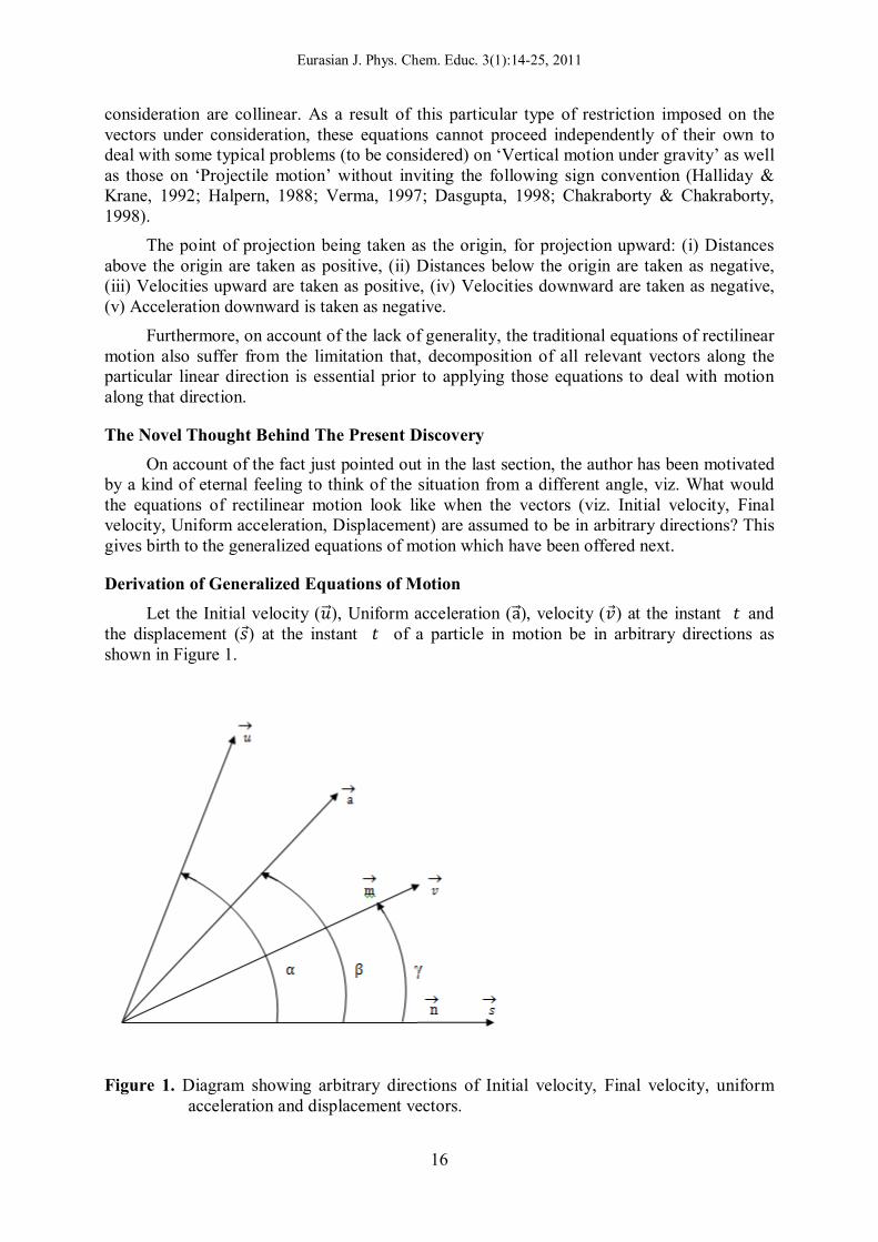
Let the Initial velocity (푢⃗), Uniform acceleration (a⃗), velocity (푣⃗) at the instant 푡 and the displacement (푠⃗) at the instant 푡 of a particle in motion be in arbitrary directions as shown in Figure 1.

Figure 1. Diagram showing arbitrary directions of Initial velocity, Final velocity, uniform

acceleration and displacement vectors.

Bhattacharjee

17

The generalized equations of rectilinear motion can then be derived as follows:

To find the generalized equation of motion connecting 풔 and 풕 :

Considering Figure 1, we have,

a cos 훽 푛⃗ =푑푑푡

푑푠⃗푑푡

where 푛⃗ represents a unit vector along the direction of 푠⃗.

∴ a 푐표푠 훽 푛⃗ 푑푡 =푑푑푡

푑푠⃗푑푡 푑푡

or, a 푡 푐표푠 훽 푛⃗ = ⃗ + 퐶⃗ (1)

where 퐶⃗ is the constant vector of integration.

Now, at 푡 = 0, we have, ⃗ = 푢 cos 훼 푛⃗

Hence from equation (1) we get,

0⃗ = 푢 cos 훼 푛⃗ + 퐶⃗

or, 퐶⃗ = (−푢 cos 훼) 푛⃗ .

Substituting this expression for 퐶⃗ in equation (1) we have,

a 푡 cos β n⃗ = ⃗ − (푢 cos α) n⃗

Again integrating we get,

∫ a 푡 cos β n⃗ d푡 = ∫ ⃗ d푡 − ∫( 푢 cos α ) n ⃗ d푡

or, a cos β n⃗ = s⃗ − 푢 푡 cos α n ⃗ + 퐶⃗ (2)


Again at 푡 = 0, we have, s⃗ = 0⃗. Hence from equation (2) we get,

퐶⃗ = 0⃗

It then follows from equation (2) that


18

a cos β n⃗ = s⃗ − 푢 푡 cos α n ⃗

or, s n⃗ = 푢 푡 cos α + a cos β n ⃗

∴ s = 푢 푡 cos α + a cos β (A)

which is the required generalized equation of motion.

To find the generalized equation of motion connecting 푣 and 푡 :


a cos(β − γ) m⃗ = ⃗

where 푚⃗ is a unit vector along the direction of 푣⃗.

∴ ∫ a cos(β − γ) m⃗ d푡 = ∫ ⃗ d푡

or, a 푡 cos (β − γ) m⃗ = 푣⃗ + 퐶⃗ (3)


Now, at 푡 = 0, we have, 푣⃗ = 푢 푐표푠 (훼 − 훾)푚⃗

Hence from (3) we get,

0⃗ = 푢 cos(α − γ) m⃗ + 퐶⃗

or, 퐶⃗ = −m⃗ 푢 cos(α − γ)

Substituting this expression for 퐶⃗ in equation (3), we get,

a 푡 cos(β − γ) m⃗ = 푣⃗ − m⃗ 푢 cos(α − γ)

or, 푣 m⃗ = [푢 cos(α − γ) + a 푡 cos(β − γ)] m⃗

∴ 푣 = 푢 cos(α − γ) + a 푡 cos(β − γ) (B)


To find the generalized equation of motion connecting 푣 and 푠 :


a cos β n⃗ = [푣 cos γ n⃗]

Bhattacharjee

19

= [푣 cos γ n⃗]

or, a cos β n⃗ = n⃗ [(푣 cos γ) (푣 cos γ)]

or, ∫ a cos β n⃗ ds = n⃗ ∫ [(푣 cos γ) (푣 cos γ)]ds

or, a s cos β n⃗ = [(푣 cos γ) ] 푛⃗ + 퐶⃗ (4)


Now, when 푠 = 0, we have, 푣 cos γ = 푢 cos α . Hence from equation (4) we get,

0⃗ = [(푢 cos α) ] 푛⃗ + 퐶⃗

or, 퐶⃗ = − [(푢 cos α) ] 푛⃗

Substituting this expression for 퐶⃗ in equation (4) we get,

a s cos β n⃗ = [(푣 cos γ) − (푢 cos α) ] n⃗

or, 푣 cos2 = 푢2 cos2 α + 2 a 푠 cos β (C)


Special Cases

Case 1: When all the vectors 푢⃗, 푣⃗, a⃗ and s are collinear and directed along the same direction we have, = = = 00 and hence the generalized equations of motion (A), (B) and (C) respectively take the forms:

푣 = 푢 + a 푡 , 푠 = 푢 푡 + a 푡 and 푣 = 푢 + 2 a s

which are the familiar equations of rectilinear motion with uniform acceleration.

Case 2: When all the vectors 푢⃗, 푣⃗, a⃗ and s are collinear but the vectors 푢⃗, 푣⃗, s⃗ are similarly directed while the direction of a is just opposite to them, then in such a case we have, = =00 and =1800. Under this condition, the generalized equations of motion (A), (B) and (C) respectively take the forms:

푣 = 푢 − a 푡 , 푠 = 푢 푡 − a 푡 and 푣 = 푢 − 2 a s ,

which are the traditional equations of rectilinear motion with uniform retardation.


20

Applications of The Generalized Equations of Motion In this section, the generalized equations of motion will be employed to solve some typical problems in kinematics.

Problem 1: A stone is let fall from a balloon ascending with a velocity 32 ft/s. The stone takes 10 s to reach the ground. Find the height of the balloon at the instant the stone was released (푔 = 32 ft/푠 ).

Solution: It can be easily seen that for this problem, we have, a = 180°, b = 0°. Hence using the generalized equation of motion,

ℎ = 푢 푡 Cosα + 푔 Cos β

we get, ℎ = − 푢 푡 + 푔 푡

On putting 푢 = 32, 푡 = 10, 푔 = 32 in this equation we then obtain

ℎ = − 32x10 + x32x10

= 1280

Thus the required height of the ballon is 1280 ft.

Remark: The above problem can be solved using the traditional equation, ℎ = 푢 푡 + 푔 푡 of rectilinear motion considering at the same time the usual sign convention in this context so that the ultimate equation to be employed to solve the problem is ℎ = − 푢 푡 + 푔 푡 . It is worth mentioning that the same equation has been made use of while solving the problem with the help of generalized equation of motion.

Problem 2: From the top of a tower, a stone is thrown vertically upward with a velocity 30 ms-1 and 4 s later another stone is dropped from the same point. Both the stones reach the ground at the same time. Find the height of the tower and time of fall of the second stone (푔 = 10 ms-2)

Solution: Let the time of fall of the second stone be T sec. Then the time of fall of the first stone will be (T + 4) sec.

For the first stone, we are to make use of the generalized equation

ℎ = 푢 푡 cosα + 푔 cos β

It can be easily seen that, for this stone we have, a = 180°, b = 0°.

Hence the above generalized equation becomes

ℎ = − 푢 푡 + 푔 푡

On putting 푢 = 30, 푔 = 10, 푡 = (푇 + 4) in this equation we get,

= − 30 (T + 4) 5 (T + 4)2 (5)

Bhattacharjee

21

For the second stone, the generalized equation of motion to be employed is also


Now, for this stone, it can be easily seen that we have, α =00, b =00. Thus the above generalized equation of motion reduces to

ℎ = 푢 푡 + g 푡

On putting 푢 = , 푔 = 10, and 푡 = T in this equation we get,

= 5 T2 (6)

Eliminating from equations (5) and (6) we obtain the value of T as T = 4.

Putting this value of T in equation (6) we get = 80.

Hence the time of fall of the second stone is 4 sec and the height of the tower is 80 m.

Remark: It may be recalled that this problem can also be solved using the traditional equation, ℎ = 푢 푡 + 푔 푡 of rectilinear motion along with the relevant sign convention. But the application of the generalized equation of motion (as made above) for solving this typical problem dispenses away with the need of the usual sign convention.

Problem 3: If a stone is projected with a velocity of 78.4 m/s from the top of a pillar 98 m high at an angle of 300 with the horizontal, find the time taken by the stone to strike the ground.

Solution: The generalized equation of motion to be employed to solve this problem is


For this problem, it can be easily seen that a = 900 + 300 =1200, β = 00. Thus the above generalized equation reduces to

ℎ = − 푢 푡 + 푔 푡

On putting = 98 , 푢 = 78.4 , 푔 = 9.8 in this equation we get,

98 = 39.2 푡 4.9 푡

or, 푡 8 푡 20 = 0

Solving this equation we get the acceptable value of 푡 as 푡 = 10.

Hence the required time taken is 10 sec.

Remark: The use of the traditional equation, ℎ = 푢 푡 + 푔 푡 along with the relevant sign convention will give the same result for this problem. But using the generalized equation of motion, the need of usual sign convention can be dispensed with.


22

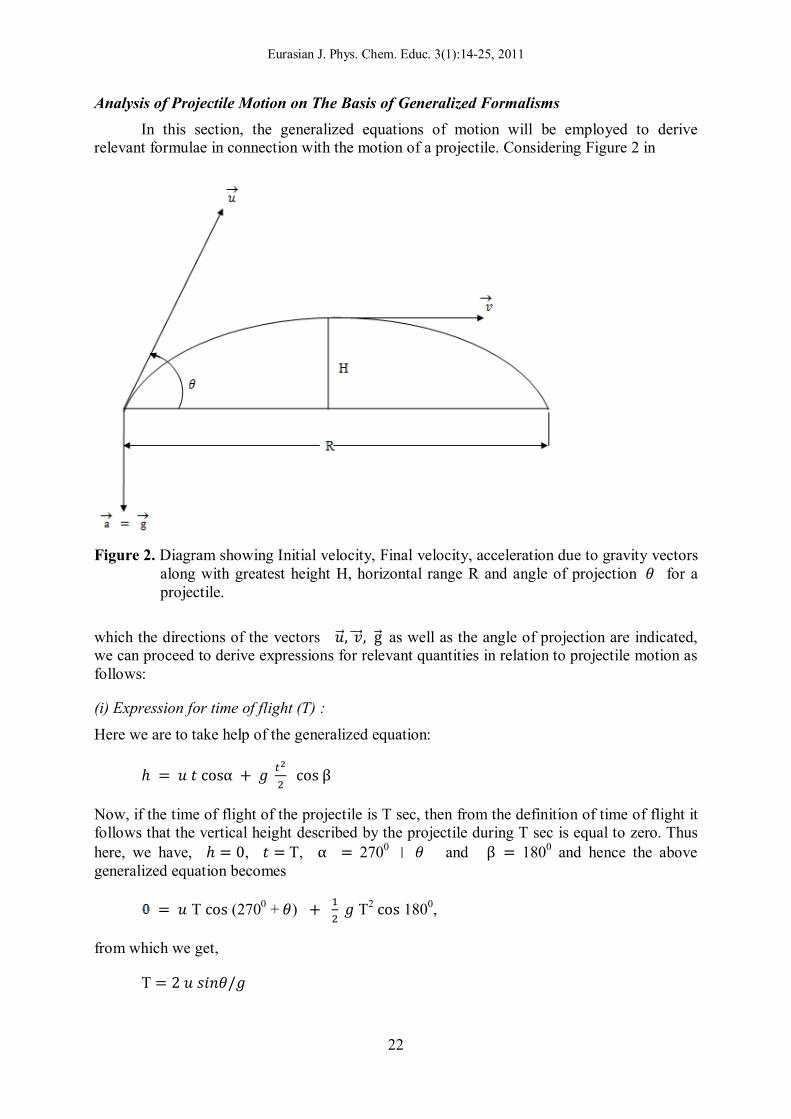
Analysis of Projectile Motion on The Basis of Generalized Formalisms In this section, the generalized equations of motion will be employed to derive relevant formulae in connection with the motion of a projectile. Considering Figure 2 in

Figure 2. Diagram showing Initial velocity, Final velocity, acceleration due to gravity vectors

along with greatest height H, horizontal range R and angle of projection 휃 for a projectile.

which the directions of the vectors 푢⃗, 푣⃗, g⃗ as well as the angle of projection are indicated, we can proceed to derive expressions for relevant quantities in relation to projectile motion as follows:

(i) Expression for time of flight (T) :

Here we are to take help of the generalized equation:


Now, if the time of flight of the projectile is T sec, then from the definition of time of flight it follows that the vertical height described by the projectile during T sec is equal to zero. Thus here, we have, ℎ = 0, 푡 = T, α = 2700 휃 and β= 1800 and hence the above generalized equation becomes

= 푢 T cos (2700 + 휃) + 푔 T2 cos 1800,

from which we get,

T = 2 푢 푠푖푛휃/푔

Bhattacharjee

23

(ii) Expression for horizontal range (R) :

Here we are to make use of the generalized equation

푠 = 푢 푡 cosα + a cos β

In this case, 푠 = R, 푡 = T, a = 푔, α = 휃 and β = 2700. Under this condition the above generalized equation becomes

R = 푢 T cos 휃 + 푔 T2 cos 2700

or, R = 푢 T cos휃

or, R = 푢 ( ) cos휃 [Putting the expression for time of flight T]

R = 푢 푠푖푛2휃/g

(iii) Expression for greatest height (H) attained :

In this case we are to take help of the generalized equation

푣2 cos 2훾 푢2 푐표푠 훼 + 2 a 푠 cos β

Here, 훼 = 270° + 휃, β=1800, g = 2700, 푠 = H and a = 푔 . Thus the above generalized equation reduces to

푣 푐표푠 2700 = 푢2 푐표푠 (2700 휃 ) 2 푔 H cos 1800,

from which we get,

H = 푢 푠푖푛 휃 /2푔

(iv) Expression for time to reach the greatest height :

Here the generalized equation to be employed is

푠 = 푢 푡 cosα + a cos β

In this case, 푠 = H = 푢 푠푖푛 휃 /2푔 ,

푡 = 푡1 (say), a = g, 훼 = 270° + 휃 and β =1800. Hence the above generalized equation becomes

푢 푠푖푛 휃 /2푔 = 푢 푡1 cos (2700 휃) 푔 푡1 2 cos 1800

Solving this quadratic equation in 푡1 we get,

푡 = 푢 푠푖푛 휃/푔


24

Conclusion The discovery of a set of generalized equations of rectilinear motion has been reported

in this paper. The key idea behind the present discovery lies in considering the velocity, acceleration and displacement vectors to be in arbitrary directions. The generalized formalisms developed are clearer leaving no room for confusion.

Remarkable features of the present discovery must be sought in the following: (i) The generalized equations of motion discovered as well as the underlying thought behind

the present discovery are both novel and original. (ii) The generalized equations of motion developed are self sufficient in respect of problem

solving and it is exclusively because of the said fact that they can be employed to solve typical problems of kinematics thereby getting rid of the need of using ambiguous sign convention for solving such typical problems on the basis of the traditional equations of kinematics.

(iii) Equations of motion for all cases of real practical relevance in kinematics are derivable from the generalized equations of motion developed with substitution of appropriate values for the angles 훼, 훽, 훾.

(iv) The generalized formalisms developed are very much likely to enrich the subject classical mechanics beyond what is available in standard literature.

(v) In order to establish a bridge between theory and practice, theoretical Physics should not stand on mathematical tools which make use of unrealistic conventions. It is a high time to get rid of such conventions. From that point of view also the present research work deserves special attention. This is because by using the generalized equations of motion developed, the need of using the ambiguous sign convention to solve typical problems of classical mechanics following the traditional scheme could be dispensed with.

(vi) It is worth mentioning here that, based on the generalized formalisms, Newton’s second law of motion (F = ma) must assume a most generalized form which can be readily developed.

Although the present paper reports on an important discovery of elementary classical mechanics, it is closely related to Physics Education as well. The novel formalisms developed and the application results offered may be used to teach Kinematics in a more clear and unambiguous manner thereby getting rid of the need of the traditional technique.

References

Bansal, R.K. (2010). A text book of Engineering Mechanics, India : Laxmi Publisher. Bhavikatti, S.S. & Rajashekarappa, K.G. (2008). Engineering Mechanics, India : New Age

International Publisher. Chakraborty, A. & Chakraborty, N. (1998). Problems in Physics, Vol. 1, India: Kalimata

Pustakalaya. Dasgupta, C.R. (1998). A text book of Physics (Part 1), India : Book Syndicate Pvt. Ltd. .

Den Hartog, J.P. (1948). Mechanics, Dover Publications, Inc. Halpern, A. (1988). Schaum’s solved Problems Series, McGraw-Hill Book Company.

Hewitt, P.G. (2007). Conceptual Physics, Addison Wesley.

Bhattacharjee

25

Hibbeler, R.C. (2009). Engineering Mechanics : Dynamics, Prentice Hall.

Kittel, C., Walter, D., Knight, W.D. & Ruderman, M.A. (1965). Mechanics, Tata McGraw-Hill Publishing Company Ltd..

Poorman, A.P. (1949). Applied Mechanics, McGraw-Hill Book Company, Inc.. Pratap, R. & Ruina, A. (2009). Introduction to Statics and Dynamics, Cornell University.

Resnick, R., Halliday, D. & Krane, S. (1992). John Wiley and Sons. Verma, H.C. (1997). Concepts of Physics, India: Bharati Bhawan.

Documents

Discovering the Generalized Equations of Motion