Discovering governing equations from data:Sparse identification of nonlinear dynamical systems

Steven L. Brunton1∗, Joshua L. Proctor2, J. Nathan Kutz3

1 Department of Mechanical Engineering, University of Washington, Seattle, WA 98195, United States2Institute for Disease Modeling, Bellevue, WA 98004, United States

3 Department of Applied Mathematics, University of Washington, Seattle, WA 98195, United States

AbstractThe ability to discover physical laws and governing equations from data is one of hu-

mankind’s greatest intellectual achievements. A quantitative understanding of dynamic con-straints and balances in nature has facilitated rapid development of knowledge and enabledadvanced technological achievements, including aircraft, combustion engines, satellites, andelectrical power. In this work, we combine sparsity-promoting techniques and machine learn-ing with nonlinear dynamical systems to discover governing physical equations from measure-ment data. The only assumption about the structure of the model is that there are only a fewimportant terms that govern the dynamics, so that the equations are sparse in the space of pos-sible functions; this assumption holds for many physical systems. In particular, we use sparseregression to determine the fewest terms in the dynamic governing equations required to accu-rately represent the data. The resulting models are parsimonious, balancing model complexitywith descriptive ability while avoiding overfitting. We demonstrate the algorithm on a widerange of problems, from simple canonical systems, including linear and nonlinear oscillatorsand the chaotic Lorenz system, to the fluid vortex shedding behind an obstacle. The fluid ex-ample illustrates the ability of this method to discover the underlying dynamics of a systemthat took experts in the community nearly 30 years to resolve. We also show that this methodgeneralizes to parameterized, time-varying, or externally forced systems.

Keywords– Dynamical systems, Sparse regression, System identification, Compressed sensing.

1 Introduction

Extracting physical laws from data is a central challenge in many diverse areas of science and en-gineering. There are many critical data-driven problems, such as understanding cognition fromneural recordings, inferring patterns in climate, determining stability of financial markets, predict-ing and suppressing the spread of disease, and controlling turbulence for greener transportationand energy. With abundant data and elusive laws, it is likely that data-driven discovery of dy-namics will continue to play an increasingly important role in these efforts.

Advances in machine learning [19] and data science [29, 21] have promised a renaissance inthe analysis and understanding of complex data, extracting patterns in vast multimodal data thatis beyond the ability of humans to grasp. However, despite the rapid development of tools tounderstand static data based on statistical relationships, there has been slow progress in distill-ing physical models of dynamic processes from big data. This has limited the ability of data∗ Corresponding author. Tel.: +1 (609)-921-6415.E-mail address: sbrunton@uw.edu (S.L. Brunton).

1

arX

iv:1

509.

0358

0v1

[m

ath.

DS]

11

Sep

2015

science models to extrapolate the dynamics beyond the attractor where they were sampled andconstructed.

An analogy may be drawn with the discoveries of Kepler and Newton. Kepler, equipped withthe most extensive and accurate planetary data of the era, developed a data-driven model for themotion of the planets, resulting in his famous elliptic orbits. However, this was an attractor basedview of the world, and it did not explain the fundamental dynamic relationships that give riseto planetary orbits, or provide a model for how these bodies react when perturbed. Newton, incontrast, discovered a dynamic relationship between momentum and energy that described theunderlying processes responsible for these elliptic orbits. This dynamic model may be generalizedto predict behavior in regimes where no data was collected. Newton’s model has proven remark-ably robust for engineering design, making it possible to land a spacecraft on the moon, whichwould not have been possible using Kepler’s model alone.

A seminal breakthrough by Schmidt and Lipson [4, 40] has resulted in a new approach to de-termine the underlying structure of a nonlinear dynamical system from data. This method usessymbolic regression (i.e., genetic programming [22]) to find nonlinear differential equations, andit balances complexity of the model, measured in the number of terms, with model accuracy. Theresulting model identification realizes a long-sought goal of the physics and engineering commu-nities to discover dynamical systems from data. However, symbolic regression is expensive, doesnot scale well to large systems of interest, and may be prone to overfitting unless care is taken toexplicitly balance model complexity with predictive power. In [40], the Pareto front is used to findparsimonious models in a large family of candidate models.

In this work, we re-envision the dynamical system discovery problem from an entirely newperspective of sparse regression [42, 14, 18] and compressed sensing [12, 8, 9, 7, 2, 43]. In particular,we leverage the fact that most physical systems have only a few relevant terms that define thedynamics, making the governing equations sparse in a high-dimensional nonlinear function space.Before the advent of compressive sampling, and related sparsity-promoting methods, determiningthe few non-zero terms in a nonlinear dynamical system would have involved a combinatorialbrute-force search, meaning that the methods would not scale to larger problems with Moore’slaw. However, powerful new theory guarantees that the sparse solution may be determined withhigh-probability using convex methods that do scale favorably with problem size. The resultingnonlinear model identification inherently balances model complexity (i.e., sparsity of right handside dynamics) with accuracy, and the underlying convex optimization algorithms ensure that themethod will be applicable to large-scale problems.

The method described here shares some similarity to the recent dynamic mode decomposition(DMD), which is a linear dynamic regression [36, 39]. DMD is an example of an equation-freemethod [20], since it only relies on measurement data, but not on knowledge of the governingequations. Recent advances in the extended DMD have developed rigorous connections betweenDMD built on nonlinear observable functions and the Koopman operator theory for nonlineardynamical systems [36, 30]. However, there is currently no theory for which nonlinear observ-able functions to use, so that assumptions must be made on the form of the dynamical system.In contrast, the method developed here results in a sparse, nonlinear regression that automaticallydetermines the relevant terms in the dynamical system. The trend to exploit sparsity in dynamicalsystems is recent but growing [38, 33, 25, 6, 35, 1]. In this work, promoting sparsity in the dynam-ics results in parsimonious natural laws.

2

2 Background

There is a long and fruitful history of modeling dynamics from data, resulting in powerful tech-niques for system identification [23]. Many of these methods arose out of the need to understandcomplex flexible structures, such as the Hubble space telescope or the international space station.The resulting models have been widely applied in nearly every branch of engineering and appliedmathematics, most notably for model-based feedback control. However, methods for system iden-tification typically require assumptions on the form of the model, and most often result in lineardynamics, limiting their effectiveness to small amplitude transient perturbations around a fixedpoint of the dynamics [15].

This work diverges from the seminal work on system identification, and instead builds onsymbolic regression and sparse representation. In particular, symbolic regression is used to findnonlinear functions describing the relationships between variables and measured dynamics (i.e.,time derivatives). Traditionally, model complexity is balanced with describing capability usingparsimony arguments such as the Pareto front. Here, we use sparse representation to determinethe relevant model terms in an efficient and scalable framework.

2.1 Symbolic regression and machine learning

Symbolic regression involves the determination of a function that relates input–output data, and itmay be viewed as a form of machine learning. Typically, the function is determined using geneticprogramming, which is an evolutionary algorithm that builds and tests candidate functions out ofsimple building blocks [22]. These functions are then modified according to a set of evolutionaryrules and generations of functions are tested until a pre-determined accuracy is achieved.

Recently, symbolic regression has been applied to data from dynamical systems, and ordinarydifferential equations were discovered from measurement data [40]. Because it is possible to over-fit with symbolic regression and genetic programming, a parsimony constraint must be imposed,and in [40], they accept candidate equations that are at the Pareto front of complexity.

2.2 Sparse representation and compressive sensing

In many regression problems, only a few terms in the regression are important, and a sparse featureselection mechanism is required. For example, consider data measurements y ∈ Rm that maybe a linear combination of columns from a feature library Θ ∈ Rm×p; the linear combination ofcolumns is given by entries of the vector ξ ∈ Rp so that:

y = Θξ. (1)

Performing a standard regression to solve for ξ will result in a solution with nonzero contributionsin each element. However, if sparsity of ξ is desired, so that most of the entries are zero, then it ispossible to add an L1 regularization term to the regression, resulting in the LASSO [14, 18, 42]:

ξ = argminξ′

‖Θξ′ − y‖2 + λ‖ξ′‖1. (2)

The parameter λ weights the sparsity constraint. This formulation is closely related to the com-pressive sensing framework, which allows for the sparse vector ξ to be determined from rela-tively few incoherent random measurements [12, 8, 9, 7, 2, 43]. The sparse solution ξ to Eq. 1 mayalso be used for sparse classification schemes, such as the sparse representation for classification(SRC) [44]. Importantly, the compressive sensing and sparse representation architectures are con-vex and scale well to large problems, as opposed to brute-force combinatorial alternatives.

3

3 Sparse identification of nonlinear dynamics (SINDy)

In this work, we are concerned with identifying the governing equations that underly a physicalsystem based on data that may be realistically collected in simulations or experiments. Generically,we seek to represent the system as a nonlinear dynamical system

x(t) = f(x(t)). (3)

The vector x(t) =[x1(t) x2(t) · · · xn(t)

]T ∈ Rn represents the state of the system at time t,and the nonlinear function f(x(t)) represents the dynamic constraints that define the equations ofmotion of the system. In the following sections, we will generalize Eq. (3) to allow the dynamics fto vary in time, and also with respect to a set of bifurcation parameters µ ∈ Rq.

The key observation in this paper is that for many systems of interest, the function f oftenconsists of only a few terms, making it sparse in the space of possible functions. For example,the Lorenz system in Eq. (22c) has very few terms in the space of polynomial functions. Recentadvances in compressive sensing and sparse regression make this viewpoint of sparsity favorable,since it is now possible to determine which right hand side terms are non-zero without performinga computationally intractable brute-force search.

To determine the form of the function f from data, we collect a time-history of the state x(t)and its derivative x(t) sampled at a number of instances in time t1, t2, · · · , tm. These data are thenarranged into two large matrices:

X =

xT (t1)xT (t2)

...xT (tm)

=

state−−−−−−−−−−−−−−−−−−−−−−−−→

x1(t1) x2(t1) · · · xn(t1)x1(t2) x2(t2) · · · xn(t2)

......

. . ....

x1(tm) x2(tm) · · · xn(tm)

y

time

(4a)

X =

xT (t1)xT (t2)

...xT (tm)

=

x1(t1) x2(t1) · · · xn(t1)x1(t2) x2(t2) · · · xn(t2)

......

. . ....

x1(tm) x2(tm) · · · xn(tm)

. (4b)

Next, we construct an augmented library Θ(X) consisting of candidate nonlinear functions of thecolumns of X. For example, Θ(X) may consist of constant, polynomial and trigonometric terms:

Θ(X) =

1 X XP2 XP3 · · · sin(X) cos(X) sin(2X) cos(2X) · · ·

. (5)

Here, higher polynomials are denoted as XP2 ,XP3 , etc. For example, XP2 denotes the quadraticnonlinearities in the state variable x, given by:

XP2 =

x21(t1) x1(t1)x2(t1) · · · x22(t1) x2(t1)x3(t1) · · · x2n(t1)x21(t2) x1(t2)x2(t2) · · · x22(t2) x2(t2)x3(t2) · · · x2n(t2)

......

. . ....

.... . .

...x21(tm) x1(tm)x2(tm) · · · x22(tm) x2(tm)x3(tm) · · · x2n(tm)

. (6)

4

X ⇥(X)

⌅

⇥(X) =

2666666666666666664

· · ·

3777777777777777775

. (27)

⇥(X) =

2666666666666666664

3777777777777777775

. (28)

21

⇥(X) =

2666666666666666664

· · ·

3777777777777777775

. (27)

⇥(X) =

2666666666666666664

3777777777777777775

. (28)

21

1 x y z x2 xy xz y2 z5

⇥(X) =

2666666666666666664

· · ·

3777777777777777775

. (27)

⇥(X) =

2666666666666666664

3777777777777777775

26666666666666666666666666664

37777777777777777777777777775

26666666666666666666666666664

37777777777777777777777777775

. (28)

21

⇥(X) =

2666666666666666664

· · ·

3777777777777777775

. (27)

⇥(X) =

2666666666666666664

3777777777777777775

26666666666666666666666666664

37777777777777777777777777775

26666666666666666666666666664

37777777777777777777777777775

. (28)

21

⇥(X) =

2666666666666666664

· · ·

3777777777777777775

. (27)

⇥(X) =

2666666666666666664

3777777777777777775

26666666666666666666666666664

37777777777777777777777777775

26666666666666666666666666664

37777777777777777777777777775

. (28)

21

x y z ⇠1 ⇠2 ⇠3

=Data In

'' 'xi_1' 'xi_2' 'xi_3' '1' [ 0] [ 0] [ 0] 'x' [-9.9996] [27.9980] [ 0] 'y' [ 9.9998] [-0.9997] [ 0] 'z' [ 0] [ 0] [-2.6665] 'xx' [ 0] [ 0] [ 0] 'xy' [ 0] [ 0] [ 1.0000] 'xz' [ 0] [-0.9999] [ 0] 'yy' [ 0] [ 0] [ 0] 'yz' [ 0] [ 0] [ 0] ... ... ... ... 'yzzzz' [ 0] [ 0] [ 0] 'zzzzz' [ 0] [ 0] [ 0]

Sparse Coefficients of Dynamics

time

⇥(X) =

2666666666666666664

· · ·

3777777777777777775

. (27)

⇥(X) =

2666666666666666664

3777777777777777775

26666666666666666666666666664

37777777777777777777777777775

26666666666666666666666666664

37777777777777777777777777775

. (28)

21

⇥(X) =

2666666666666666664

· · ·

3777777777777777775

. (27)

⇥(X) =

2666666666666666664

3777777777777777775

26666666666666666666666666664

37777777777777777777777777775

26666666666666666666666666664

37777777777777777777777777775

. (28)

21

⇥(X) =

2666666666666666664

· · ·

3777777777777777775

. (27)

⇥(X) =

2666666666666666664

3777777777777777775

26666666666666666666666666664

37777777777777777777777777775

26666666666666666666666666664

37777777777777777777777777775

. (28)

21

⇥(X) =

2666666666666666664

· · ·

3777777777777777775

. (27)

⇥(X) =

2666666666666666664

3777777777777777775

26666666666666666666666666664

37777777777777777777777777775

26666666666666666666666666664

37777777777777777777777777775

. (28)

21

⇥(X) =

2666666666666666664

· · ·

3777777777777777775

. (27)

⇥(X) =

2666666666666666664

3777777777777777775

. (28)

21

⇥(X) =

2666666666666666664

· · ·

3777777777777777775

. (27)

⇥(X) =

2666666666666666664

3777777777777777775

. (28)

21

⇥(X) =

2666666666666666664

· · ·

3777777777777777775

. (27)

⇥(X) =

2666666666666666664

3777777777777777775

26666666666666666666666666664

37777777777777777777777777775

26666666666666666666666666664

37777777777777777777777777775

. (28)

21

⇥(X) =

2666666666666666664

· · ·

3777777777777777775

. (27)

⇥(X) =

2666666666666666664

3777777777777777775

26666666666666666666666666664

37777777777777777777777777775

26666666666666666666666666664

37777777777777777777777777775

. (28)

21

=

⇥(X) =

2666666666666666664

· · ·

3777777777777777775

. (27)

⇥(X) =

2666666666666666664

3777777777777777775

. (28)

21

⇥(X) =

2666666666666666664

· · ·

3777777777777777775

. (27)

⇥(X) =

2666666666666666664

3777777777777777775

. (28)

21

⇥(X) =

2666666666666666664

· · ·

3777777777777777775

. (27)

⇥(X) =

2666666666666666664

3777777777777777775

26666666666666666666666666664

37777777777777777777777777775

26666666666666666666666666664

37777777777777777777777777775

. (28)

21

⇥(X) =

2666666666666666664

· · ·

3777777777777777775

. (27)

⇥(X) =

2666666666666666664

3777777777777777775

26666666666666666666666666664

37777777777777777777777777775

26666666666666666666666666664

37777777777777777777777777775

. (28)

21

=

⇥(X) =

2666666666666666664

· · ·

3777777777777777775

. (27)

⇥(X) =

2666666666666666664

3777777777777777775

26666666666666666666666666664

37777777777777777777777777775

26666666666666666666666666664

37777777777777777777777777775

. (28)

21

⇥(X) =

2666666666666666664

· · ·

3777777777777777775

. (27)

⇥(X) =

2666666666666666664

3777777777777777775

26666666666666666666666666664

37777777777777777777777777775

26666666666666666666666666664

37777777777777777777777777775

. (28)

21

⇥(X) =

2666666666666666664

· · ·

3777777777777777775

. (27)

⇥(X) =

2666666666666666664

3777777777777777775

. (28)

21

⇥(X) =

2666666666666666664

· · ·

3777777777777777775

. (27)

⇥(X) =

2666666666666666664

3777777777777777775

. (28)

21

⇥(X) =

2666666666666666664

· · ·

3777777777777777775

. (27)

⇥(X) =

2666666666666666664

3777777777777777775

26666666666666666666666666664

37777777777777777777777777775

26666666666666666666666666664

37777777777777777777777777775

. (28)

21

⇥(X) =

2666666666666666664

· · ·

3777777777777777775

. (27)

⇥(X) =

2666666666666666664

3777777777777777775

26666666666666666666666666664

37777777777777777777777777775

26666666666666666666666666664

37777777777777777777777777775

. (28)

21

z xy ⇠3zx y xz ⇠2y⇠1x yx

=

III. Identified System

4.2 Example 2: Lorenz system (Nonlinear ODE)

Here, we consider the nonlinear Lorenz system to explore the identification of chaotic dynamics:

x = �(y � x) (18)y = x(⇢� z) � y (19)z = xy � �z. (20)

For this example, we use the standard parameters � = 10,� = 8/3, ⇢ = 28, with an initial condition⇥x y z

⇤T=

⇥�8 7 27

⇤T .

24x(t) y(t) z(t) x(t)2 x(t)y(t) x(t)z(t) y(t)2 y(t)z(t) z(t)2 · · ·

35 (21)

Full Simulation

0

25

50

z

-20 0 20x -500

50y

Identified System, ⌘ = 0.01

0

25

50

z

-20 0 20x -500

50y

Identified System, ⌘ = 10

0

25

50

z

-20 0 20x -500

50y

0

25

50

z

-20 0 20x -500

50y

0

25

50

z

-20 0 20x -500

50y

0

25

50

z

-20 0 20x -500

50y

Figure 3: Trajectories of the Lorenz system for short-time integration from t = 0 to t = 20 (top)and long-time integration from t = 0 to t = 250 (bottom). The full dynamics (left) are comparedwith the sparse identified systems (middle, right) for various additive noise. The trajectories arecolored by �t, the adaptive Runge-Kutta time step. This color is a proxy for local sensitivity.

10

x = ⇥(xT )⇠1

y = ⇥(xT )⇠2

z = ⇥(xT )⇠3

II. Sparse Regression to Solve for Active Terms in the Dynamics

4.2 Example 2: Lorenz system (Nonlinear ODE)

Here, we consider the nonlinear Lorenz system to explore the identification of chaotic dynamics:

x = �(y � x) (18)y = x(⇢� z) � y (19)z = xy � �z. (20)

For this example, we use the standard parameters � = 10,� = 8/3, ⇢ = 28, with an initial condition⇥x y z

⇤T=

⇥�8 7 27

⇤T .

24x(t) y(t) z(t) x(t)2 x(t)y(t) x(t)z(t) y(t)2 y(t)z(t) z(t)2 · · ·

35 (21)

Full Simulation

0

25

50

z

-20 0 20x -500

50y

Identified System, ⌘ = 0.01

0

25

50

z

-20 0 20x -500

50y

Identified System, ⌘ = 10

0

25

50

z

-20 0 20x -500

50y

0

25

50

z

-20 0 20x -500

50y

0

25

50

z

-20 0 20x -500

50y

0

25

50

z

-20 0 20x -500

50y

Figure 3: Trajectories of the Lorenz system for short-time integration from t = 0 to t = 20 (top)and long-time integration from t = 0 to t = 250 (bottom). The full dynamics (left) are comparedwith the sparse identified systems (middle, right) for various additive noise. The trajectories arecolored by �t, the adaptive Runge-Kutta time step. This color is a proxy for local sensitivity.

10

4.2 Example 2: Lorenz system (Nonlinear ODE)

Here, we consider the nonlinear Lorenz system to explore the identification of chaotic dynamics:

x = �(y � x) (18)y = x(⇢� z) � y (19)z = xy � �z. (20)

For this example, we use the standard parameters � = 10,� = 8/3, ⇢ = 28, with an initial condition⇥x y z

⇤T=

⇥�8 7 27

⇤T .

24x(t) y(t) z(t) x(t)2 x(t)y(t) x(t)z(t) y(t)2 y(t)z(t) z(t)2 · · ·

35 (21)

Full Simulation

0

25

50

z

-20 0 20x -500

50y

Identified System, ⌘ = 0.01

0

25

50

z

-20 0 20x -500

50y

Identified System, ⌘ = 10

0

25

50

z

-20 0 20x -500

50y

0

25

50

z

-20 0 20x -500

50y

0

25

50

z

-20 0 20x -500

50y

0

25

50

z

-20 0 20x -500

50y

Figure 3: Trajectories of the Lorenz system for short-time integration from t = 0 to t = 20 (top)and long-time integration from t = 0 to t = 250 (bottom). The full dynamics (left) are comparedwith the sparse identified systems (middle, right) for various additive noise. The trajectories arecolored by �t, the adaptive Runge-Kutta time step. This color is a proxy for local sensitivity.

10

I. True Lorenz System

Model O

ut

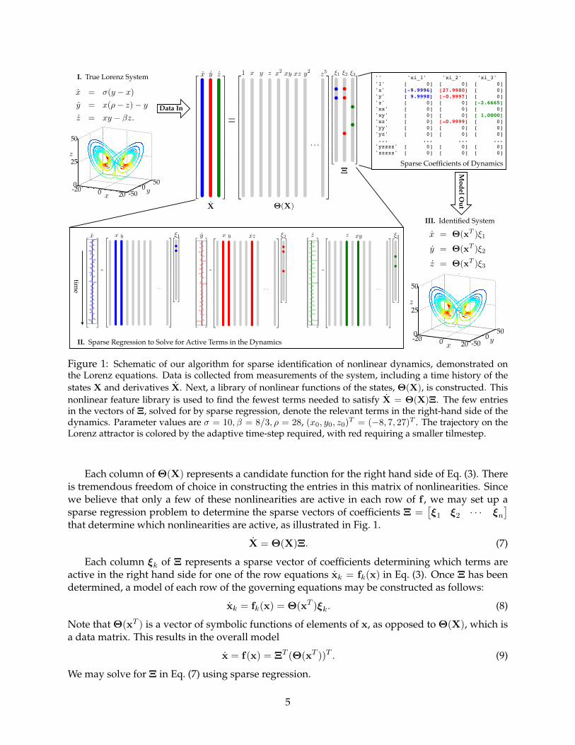
Figure 1: Schematic of our algorithm for sparse identification of nonlinear dynamics, demonstrated onthe Lorenz equations. Data is collected from measurements of the system, including a time history of thestates X and derivatives X. Next, a library of nonlinear functions of the states, Θ(X), is constructed. Thisnonlinear feature library is used to find the fewest terms needed to satisfy X = Θ(X)Ξ. The few entriesin the vectors of Ξ, solved for by sparse regression, denote the relevant terms in the right-hand side of thedynamics. Parameter values are σ = 10, β = 8/3, ρ = 28, (x0, y0, z0)T = (−8, 7, 27)T . The trajectory on theLorenz attractor is colored by the adaptive time-step required, with red requiring a smaller tilmestep.

Each column of Θ(X) represents a candidate function for the right hand side of Eq. (3). Thereis tremendous freedom of choice in constructing the entries in this matrix of nonlinearities. Sincewe believe that only a few of these nonlinearities are active in each row of f , we may set up asparse regression problem to determine the sparse vectors of coefficients Ξ =

[ξ1 ξ2 · · · ξn

]

that determine which nonlinearities are active, as illustrated in Fig. 1.

X = Θ(X)Ξ. (7)

Each column ξk of Ξ represents a sparse vector of coefficients determining which terms areactive in the right hand side for one of the row equations xk = fk(x) in Eq. (3). Once Ξ has beendetermined, a model of each row of the governing equations may be constructed as follows:

xk = fk(x) = Θ(xT )ξk. (8)

Note that Θ(xT ) is a vector of symbolic functions of elements of x, as opposed to Θ(X), which isa data matrix. This results in the overall model

x = f(x) = ΞT (Θ(xT ))T . (9)

We may solve for Ξ in Eq. (7) using sparse regression.

5

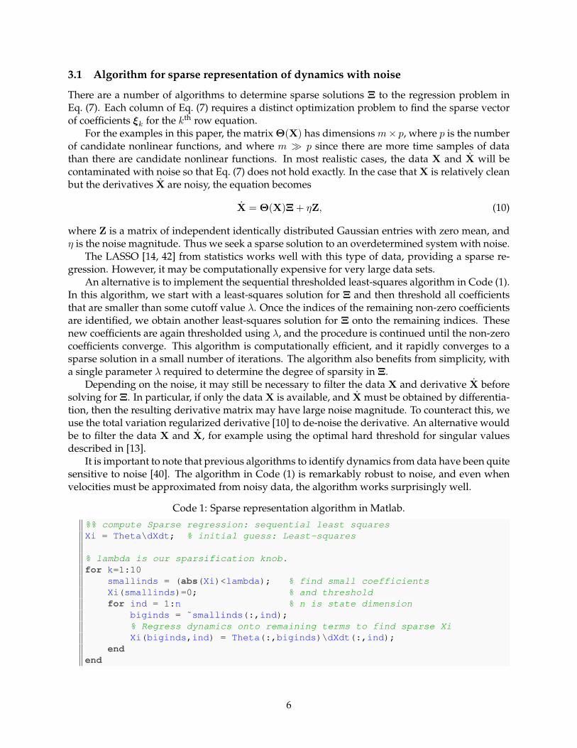
3.1 Algorithm for sparse representation of dynamics with noise

There are a number of algorithms to determine sparse solutions Ξ to the regression problem inEq. (7). Each column of Eq. (7) requires a distinct optimization problem to find the sparse vectorof coefficients ξk for the kth row equation.

For the examples in this paper, the matrix Θ(X) has dimensions m× p, where p is the numberof candidate nonlinear functions, and where m � p since there are more time samples of datathan there are candidate nonlinear functions. In most realistic cases, the data X and X will becontaminated with noise so that Eq. (7) does not hold exactly. In the case that X is relatively cleanbut the derivatives X are noisy, the equation becomes

X = Θ(X)Ξ + ηZ, (10)

where Z is a matrix of independent identically distributed Gaussian entries with zero mean, andη is the noise magnitude. Thus we seek a sparse solution to an overdetermined system with noise.

The LASSO [14, 42] from statistics works well with this type of data, providing a sparse re-gression. However, it may be computationally expensive for very large data sets.

An alternative is to implement the sequential thresholded least-squares algorithm in Code (1).In this algorithm, we start with a least-squares solution for Ξ and then threshold all coefficientsthat are smaller than some cutoff value λ. Once the indices of the remaining non-zero coefficientsare identified, we obtain another least-squares solution for Ξ onto the remaining indices. Thesenew coefficients are again thresholded using λ, and the procedure is continued until the non-zerocoefficients converge. This algorithm is computationally efficient, and it rapidly converges to asparse solution in a small number of iterations. The algorithm also benefits from simplicity, witha single parameter λ required to determine the degree of sparsity in Ξ.

Depending on the noise, it may still be necessary to filter the data X and derivative X beforesolving for Ξ. In particular, if only the data X is available, and X must be obtained by differentia-tion, then the resulting derivative matrix may have large noise magnitude. To counteract this, weuse the total variation regularized derivative [10] to de-noise the derivative. An alternative wouldbe to filter the data X and X, for example using the optimal hard threshold for singular valuesdescribed in [13].

It is important to note that previous algorithms to identify dynamics from data have been quitesensitive to noise [40]. The algorithm in Code (1) is remarkably robust to noise, and even whenvelocities must be approximated from noisy data, the algorithm works surprisingly well.

Code 1: Sparse representation algorithm in Matlab.

%% compute Sparse regression: sequential least squaresXi = Theta\dXdt; % initial guess: Least-squares

% lambda is our sparsification knob.for k=1:10

smallinds = (abs(Xi)<lambda); % find small coefficientsXi(smallinds)=0; % and thresholdfor ind = 1:n % n is state dimension

biginds = ˜smallinds(:,ind);% Regress dynamics onto remaining terms to find sparse XiXi(biginds,ind) = Theta(:,biginds)\dXdt(:,ind);

endend

6

3.2 Cross-validation to determine parsimonious sparse solution on Pareto front

To determine the sparsification parameter λ in the algorithm in Code (1), it is helpful to use theconcept of cross-validation from machine learning. It is always possible to hold back some testdata apart from the training data to test the validity of models away from training values. Inaddition, it is important to consider the balance of model complexity (given by the number ofnonzero coefficients in Ξ) with the model accuracy. There is an “elbow” in the curve of accuracyvs. complexity parameterized by λ, the so-called Pareto front. This value of λ represents a goodtradeoff between complexity and accuracy, and it is similar to the approach taken in [40].

3.3 Extensions and Connections

There are a number of extensions to the basic theory above that generalize this approach to abroader set of problems. First, the method is generalized to a discrete-time formulation, establish-ing a connection with the dynamic mode decomposition (DMD). Next, high-dimensional systemsobtained from discretized partial differential equations are considered, extending the method toincorporate dimensionality reduction techniques to handle big data. Finally, the sparse regressionframework is modified to include bifurcation parameters, time-dependence, and external forcing.

3.3.1 Discrete-time representation

The aforementioned strategy may also be implemented on discrete-time dynamical systems:

xk+1 = f(xk). (11)

There are a number of reasons to implement Eq. (11). First, many systems, such as the logisticmap in Eq. (26) are inherently discrete-time systems. In addition, it may be possible to recoverspecific integration schemes used to advance Eq. (3). The discrete-time formulation also foregoesthe calculation of a derivative from noisy data. The data collection will now involve two matricesXm−1

1 and Xm2 :

Xm−11 =

xT1xT2...

xTm−1

, Xm

2 =

xT2xT3...

xTm

. (12)

The continuous-time sparse regression problem in Eq. (7) now becomes:

Xm2 = Θ(Xm−1

1 )Ξ (13)

and the function f is the same as in Eq. (9).In the discrete setting in Eq. (11), and for linear dynamics, there is a striking resemblance to

dynamic mode decomposition. In particular, if Θ(x) = x, so that the dynamical system is linear,then Eq. (13) becomes

Xm2 = Xm−1

1 Ξ =⇒ (Xm2 )T = ΞT

(Xm−1

1

)T. (14)

This is equivalent to the DMD, which seeks a dynamic regression onto linear dynamics ΞT . Inparticular, ΞT is n×n dimensional, which may be prohibitively large for a high-dimensional statex. Thus, DMD identifies the dominant terms in the eigendecomposition of ΞT .

7

3.3.2 High-dimensional systems, partial differential equations, and dimensionality reduction

Often, the physical system of interest may be naturally represented by a partial differential equa-tion (PDE) in a few spatial variables. If data is collected from a numerical discretization or fromexperimental measurements on a spatial grid, then the state dimension n may be prohibitivelylarge. For example, in fluid dynamics, even simple two-dimensional and three-dimensional flowsmay require tens of thousands up to billions of variables to represent the discretized system.

The method described above is prohibitive for a large state dimension n, both because of thefactorial growth of Θ in n and because each of the n row equations in Eq. (8) requires a separate op-timization. Fortunately, many high-dimensional systems of interest evolve on a low-dimensionalmanifold or attractor that may be well-approximated using a dimensionally reduced low-rank ba-sis Ψ [16, 27]. For example, if data X is collected for a high-dimensional system as in Eq. (4a), it ispossible to obtain a low-rank approximation using the singular value decomposition (SVD):

XT = ΨΣV∗. (15)

In this case, the state x may be well approximated in a truncated modal basis Ψr, given by the firstr columns of Ψ from the SVD:

x ≈ Ψra, (16)

where a is an r-dimensional vector of mode coefficients. We assume that this is a good approxi-mation for a relatively low rank r. Thus, instead of using the original high-dimensional state x, itis possible to obtain a sparse representation of the Galerkin projected dynamics fP in terms of thecoefficients a:

a = fP (a). (17)

There are many choices for a low-rank basis, including proper orthogonal decomposition (POD) [3,16], based on the SVD.

3.3.3 External forcing, bifurcation parameters, and normal forms

In practice, many real-world systems depend on parameters, and dramatic changes, or bifurca-tions, may occur when the parameter is varied [15, 26]. The algorithm above is readily extendedto encompass these important parameterized systems, allowing for the discovery of normal formsassociated with a bifurcation parameter µ. First, we append µ to the dynamics:

x = f(x;µ) (18a)µ = 0. (18b)

It is then possible to identify the right hand side f(x;µ) as a sparse combination of functions ofcomponents in x as well as the bifurcation parameter µ. This idea is illustrated on two examples,the one-dimensional logistic map and the two-dimensional Hopf normal form.

Time-dependence, known external forcing or control u(t) may also be added to the dynamics:

x = f(x,u(t), t) (19a)t = 1. (19b)

This generalization makes it possible to analyze systems that are externally forced or controlled.For example, the climate is both parameterized [26] and has external forcing, including carbondioxide and solar radiation. The financial market presents another important example with forc-ing and active feedback control, in the form of regulations, taxes, and interest rates.

8

4 Results

We demonstrate the methods described in Sec. 3 on a number of canonical systems, ranging fromsimple linear and nonlinear damped oscillators, to noisy measurements of the fully chaotic Lorenzsystem, and to measurements of the unsteady fluid wake behind a circular cylinder, extending thismethod to nonlinear partial differential equations (PDEs) and high-dimensional data. Finally, weshow that bifurcation parameters may be included in the sparse models, recovering the correctnormal forms from noisy measurements of the logistic map and the Hopf normal form.

4.1 Example 1: Simple illustrative systems

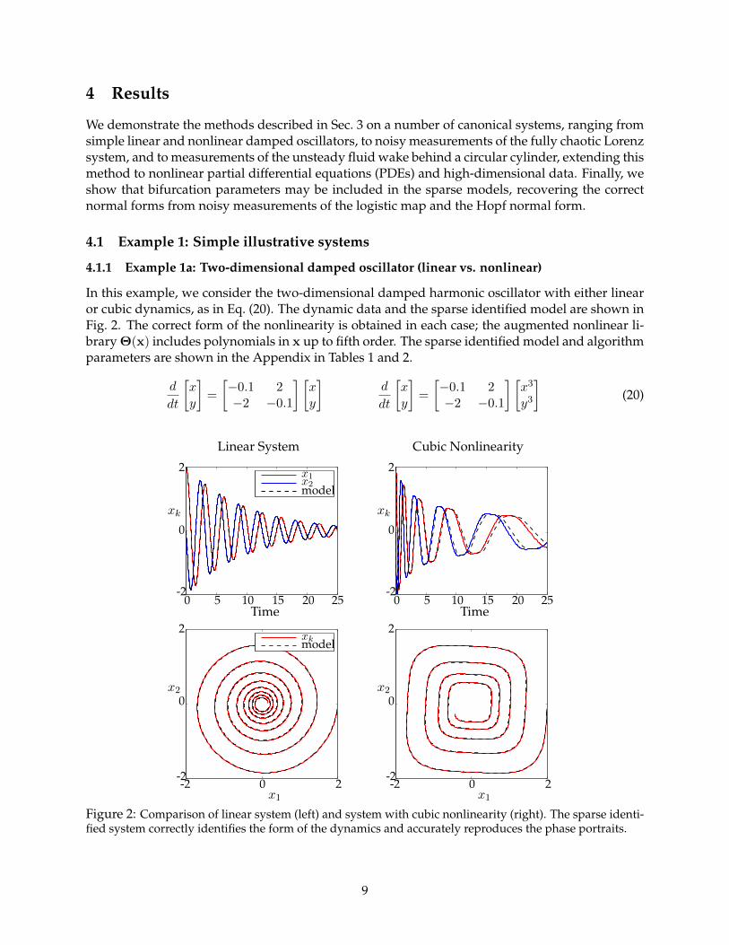
4.1.1 Example 1a: Two-dimensional damped oscillator (linear vs. nonlinear)

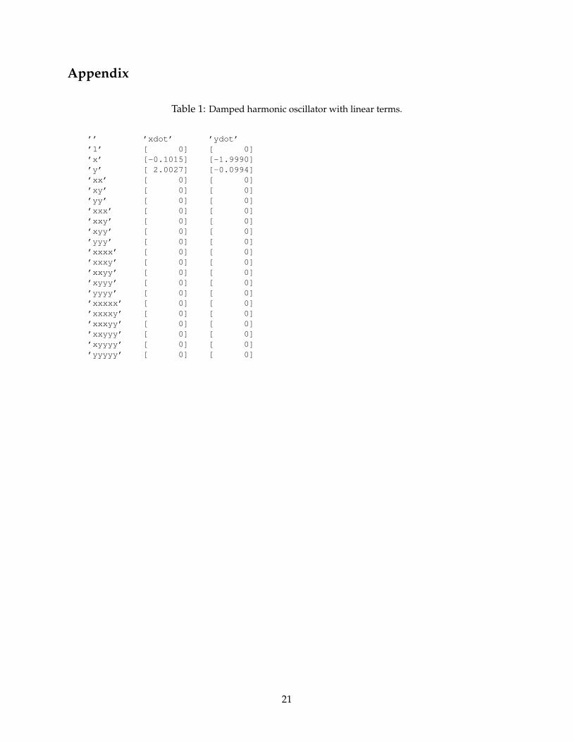
In this example, we consider the two-dimensional damped harmonic oscillator with either linearor cubic dynamics, as in Eq. (20). The dynamic data and the sparse identified model are shown inFig. 2. The correct form of the nonlinearity is obtained in each case; the augmented nonlinear li-brary Θ(x) includes polynomials in x up to fifth order. The sparse identified model and algorithmparameters are shown in the Appendix in Tables 1 and 2.

d

dt

[xy

]=

[−0.1 2−2 −0.1

] [xy

]d

dt

[xy

]=

[−0.1 2−2 −0.1

] [x3

y3

](20)

Linear System Cubic Nonlinearity

��������

0 5 10 15 20 25-2

0

2x2x1

model

Time

xk

0 5 10 15 20 25-2

0

2

Time

xk

��������

-2 0 2-2

0

2xkmodel

x1

x2

-2 0 2-2

0

2

x1

x2

Figure 2: Comparison of linear system (left) and system with cubic nonlinearity (right). The sparse identi-fied system correctly identifies the form of the dynamics and accurately reproduces the phase portraits.

9

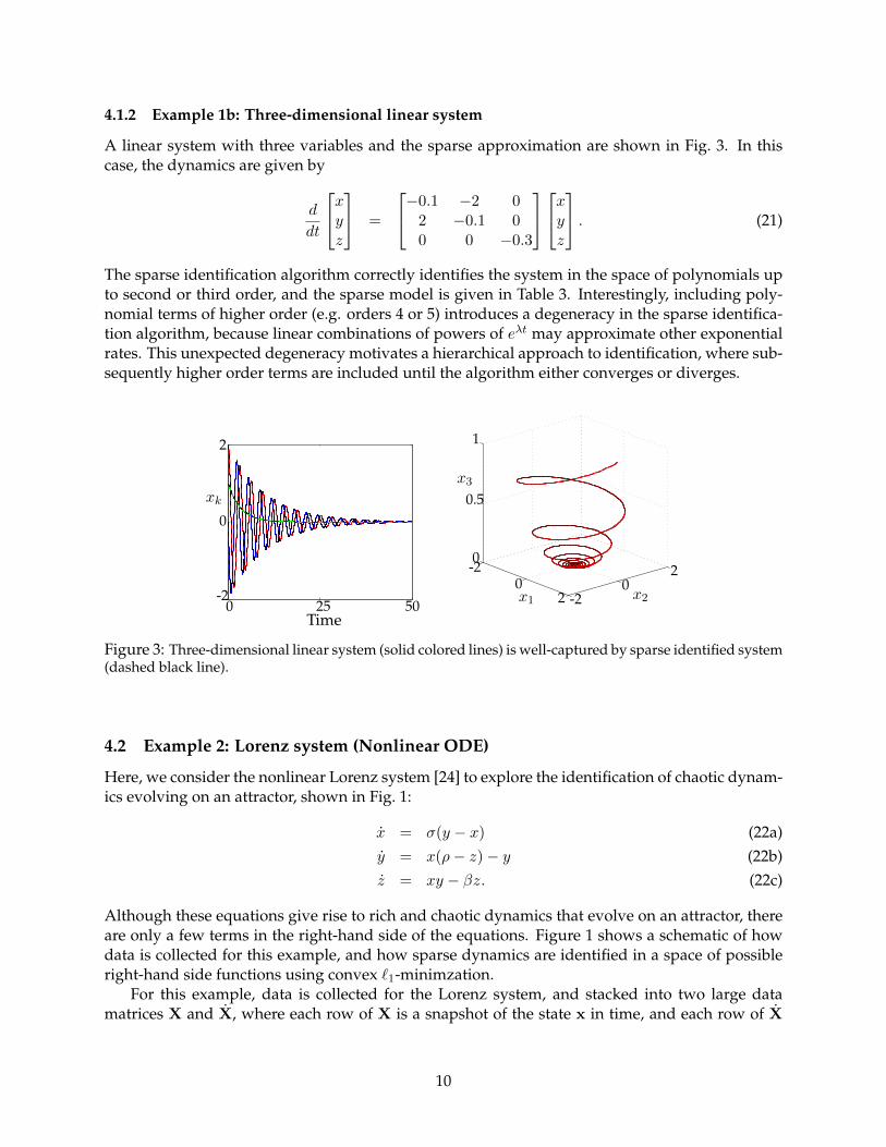
4.1.2 Example 1b: Three-dimensional linear system

A linear system with three variables and the sparse approximation are shown in Fig. 3. In thiscase, the dynamics are given by

d

dt

xyz

=

−0.1 −2 0

2 −0.1 00 0 −0.3

xyz

. (21)

The sparse identification algorithm correctly identifies the system in the space of polynomials upto second or third order, and the sparse model is given in Table 3. Interestingly, including poly-nomial terms of higher order (e.g. orders 4 or 5) introduces a degeneracy in the sparse identifica-tion algorithm, because linear combinations of powers of eλt may approximate other exponentialrates. This unexpected degeneracy motivates a hierarchical approach to identification, where sub-sequently higher order terms are included until the algorithm either converges or diverges.

0 25 50-2

0

2

Time

xk

-20

2 -20

20

0.5

1

x1 x2

x3

Figure 3: Three-dimensional linear system (solid colored lines) is well-captured by sparse identified system(dashed black line).

4.2 Example 2: Lorenz system (Nonlinear ODE)

Here, we consider the nonlinear Lorenz system [24] to explore the identification of chaotic dynam-ics evolving on an attractor, shown in Fig. 1:

x = σ(y − x) (22a)y = x(ρ− z)− y (22b)z = xy − βz. (22c)

Although these equations give rise to rich and chaotic dynamics that evolve on an attractor, thereare only a few terms in the right-hand side of the equations. Figure 1 shows a schematic of howdata is collected for this example, and how sparse dynamics are identified in a space of possibleright-hand side functions using convex `1-minimzation.

For this example, data is collected for the Lorenz system, and stacked into two large datamatrices X and X, where each row of X is a snapshot of the state x in time, and each row of X

10

is a snapshot of the time derivative of the state x in time. Here, the right-hand side dynamics areidentified in the space of polynomials Θ(X) in (x, y, z) up to fifth order:

Θ(X) =

x(t) y(t) z(t) x(t)2 x(t)y(t) x(t)z(t) y(t)2 y(t)z(t) z(t)2 · · · z(t)5

. (23)

Each column of Θ(X) represents a candidate function for the right hand side of Eq. (3), and asparse regression determines which terms are active in the dynamics, as in Fig. 1, and Eq. (7).

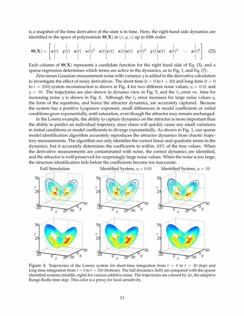
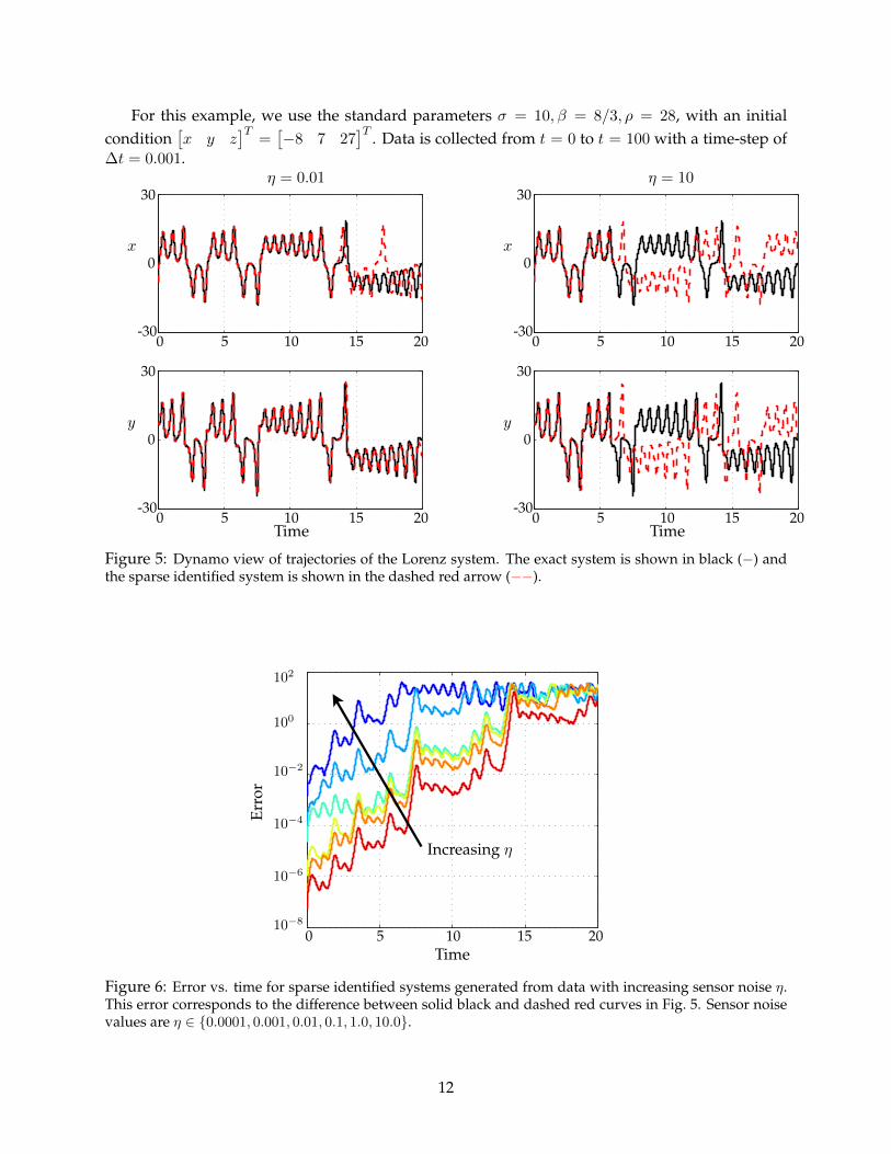
Zero-mean Gaussian measurement noise with variance η is added to the derivative calculationto investigate the effect of noisy derivatives. The short-time (t = 0 to t = 20) and long-time (t = 0to t = 250) system reconstruction is shown in Fig. 4 for two different noise values, η = 0.01 andη = 10. The trajectories are also shown in dynamo view in Fig. 5, and the `2 error vs. time forincreasing noise η is shown in Fig. 6. Although the `2 error increases for large noise values η,the form of the equations, and hence the attractor dynamics, are accurately captured. Becausethe system has a positive Lyapunov exponent, small differences in model coefficients or initialconditions grow exponentially, until saturation, even though the attractor may remain unchanged.

In the Lorenz example, the ability to capture dynamics on the attractor is more important thanthe ability to predict an individual trajectory, since chaos will quickly cause any small variationsin initial conditions or model coefficients to diverge exponentially. As shown in Fig. 1, our sparsemodel identification algorithm accurately reproduces the attractor dynamics from chaotic trajec-tory measurements. The algorithm not only identifies the correct linear and quadratic terms in thedynamics, but it accurately determines the coefficients to within .03% of the true values. Whenthe derivative measurements are contaminated with noise, the correct dynamics are identified,and the attractor is well-preserved for surprisingly large noise values. When the noise is too large,the structure identification fails before the coefficients become too inaccurate.

Full Simulation

0

25

50

z

-20 0 20x -500

50y

Identified System, η = 0.01

0

25

50

z

-20 0 20x -500

50y

Identified System, η = 10

0

25

50

z

-20 0 20x -500

50y

0

25

50

z

-20 0 20x -500

50y

0

25

50

z

-20 0 20x -500

50y

0

25

50

z

-20 0 20x -500

50y

Figure 4: Trajectories of the Lorenz system for short-time integration from t = 0 to t = 20 (top) andlong-time integration from t = 0 to t = 250 (bottom). The full dynamics (left) are compared with the sparseidentified systems (middle, right) for various additive noise. The trajectories are colored by ∆t, the adaptiveRunge-Kutta time step. This color is a proxy for local sensitivity.

11

For this example, we use the standard parameters σ = 10, β = 8/3, ρ = 28, with an initialcondition

[x y z

]T=[−8 7 27

]T . Data is collected from t = 0 to t = 100 with a time-step of∆t = 0.001.

0 5 10 15 20-30

0

30

x

η = 0.01

0 5 10 15 20-30

0

30

x

η = 10

0 5 10 15 20-30

0

30

y

Time0 5 10 15 20

-30

0

30

y

Time

Figure 5: Dynamo view of trajectories of the Lorenz system. The exact system is shown in black (−) andthe sparse identified system is shown in the dashed red arrow (−−).

0 5 10 15 2010−8

10−6

10−4

10−2

100

102

Time

Erro

r

Increasing η

Figure 6: Error vs. time for sparse identified systems generated from data with increasing sensor noise η.This error corresponds to the difference between solid black and dashed red curves in Fig. 5. Sensor noisevalues are η ∈ {0.0001, 0.001, 0.01, 0.1, 1.0, 10.0}.

12

4.3 Example 3: Fluid wake behind a cylinder (Nonlinear PDE)

The Lorenz system is a low-dimensional model of more realistic high-dimensional partial differ-ential equation (PDE) models for fluid convection in the atmosphere. Many systems of interest aregoverned by PDEs [38], such as weather and climate, epidemiology, and the power grid, to namea few. Each of these examples are characterized by big data, consisting of large spatially resolvedmeasurements consisting of millions or billions of states and spanning orders of magnitude ofscale in both space and time. However, many high-dimensional, real-world systems evolve on alow-dimensional attractor, making the effective dimension much smaller [16].

Here we generalize the sparse identification of nonlinear dynamics method to an examplein fluid dynamics that typifies many of the challenges outlined above. Data is collected for thefluid flow past a cylinder at Reynolds number 100 using direct numerical simulations of the two-dimensional Navier-Stokes equations [41, 11]. Then, the nonlinear dynamic relationship betweenthe dominant coherent structures is identified from these flow field measurements with no knowl-edge of the governing equations.

The low-Reynolds number flow past a cylinder is a particularly interesting example becauseof its rich history in fluid mechanics and dynamical systems. It has long been theorized thatturbulence may be the result of a sequence of Hopf bifurcations that occur as the Reynolds numberof the flow increases [37]. The Reynolds number is a rough measure of the ratio of inertial andviscous forces, and an increasing Reynolds number may correspond, for example, to increasingflow velocity, giving rise to more rich and intricate structures in the fluid.

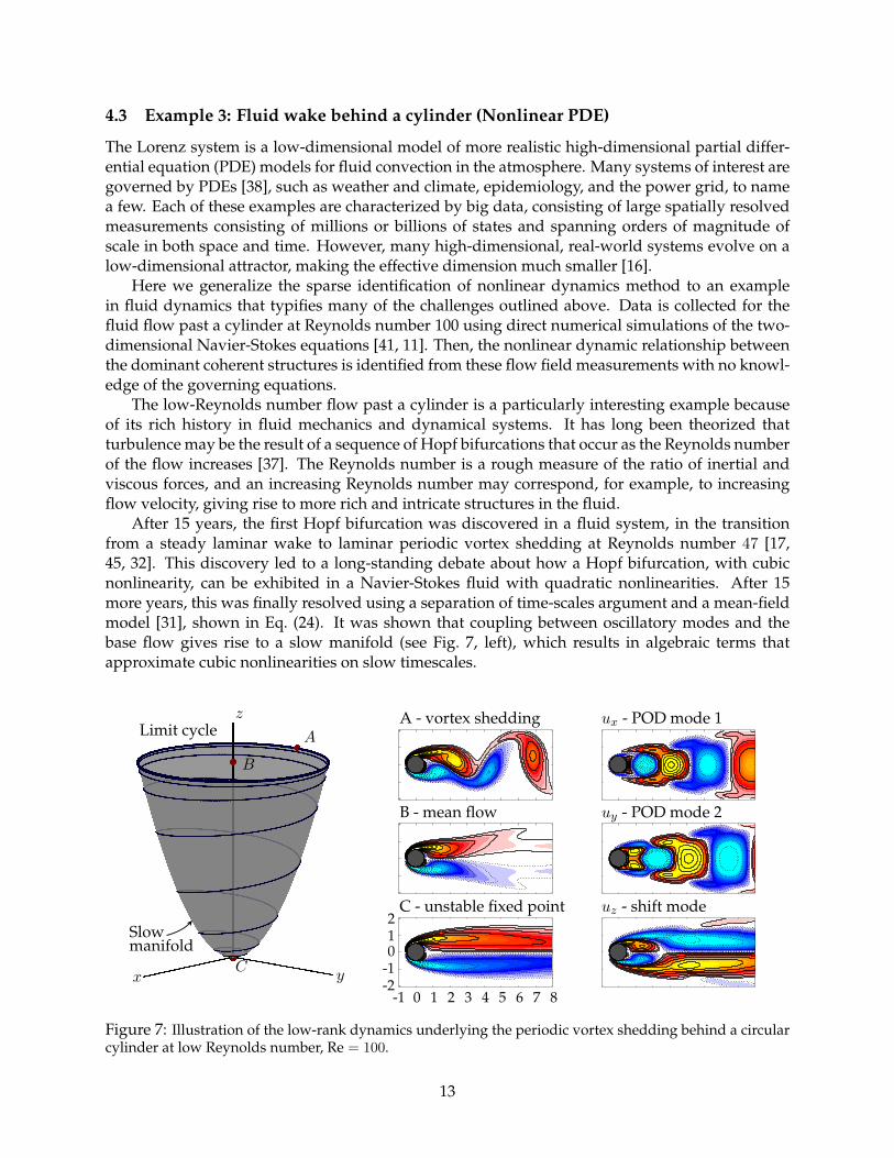
After 15 years, the first Hopf bifurcation was discovered in a fluid system, in the transitionfrom a steady laminar wake to laminar periodic vortex shedding at Reynolds number 47 [17,45, 32]. This discovery led to a long-standing debate about how a Hopf bifurcation, with cubicnonlinearity, can be exhibited in a Navier-Stokes fluid with quadratic nonlinearities. After 15more years, this was finally resolved using a separation of time-scales argument and a mean-fieldmodel [31], shown in Eq. (24). It was shown that coupling between oscillatory modes and thebase flow gives rise to a slow manifold (see Fig. 7, left), which results in algebraic terms thatapproximate cubic nonlinearities on slow timescales.

x y

z

C

A

B

Limit cycleA - vortex shedding

B - mean flow

C - unstable fixed point

ux - POD mode 1

uy - POD mode 2

uz - shift mode

Slowmanifold

-1 0 1 2 3 4 5 6 7 8-2-1012

Figure 7: Illustration of the low-rank dynamics underlying the periodic vortex shedding behind a circularcylinder at low Reynolds number, Re = 100.

13

This example provides a compelling test-case for the proposed algorithm, since the under-lying form of the dynamics took nearly three decades to uncover. Indeed, the sparse dynamicsalgorithm correctly identifies the on-attractor and off-attractor dynamics using quadratic nonlin-earities and preserves the correct slow-manifold dynamics. It is interesting to note that when theoff-attractor trajectories are not included in the system identification, the algorithm incorrectlyidentifies the dynamics using cubic nonlinearities, and fails to correctly identify the dynamicsassociated with the shift mode, which connects the mean flow to the unstable steady state.

4.3.1 Direct numerical simulation

The direct numerical simulation involves a fast multi-domain immersed boundary projectionmethod [41, 11]. Four grids are used, each with a resolution of 450 × 200, with the finest gridhaving dimensions of 9× 4 cylinder diameters and the largest grid having dimensions of 72× 32diameters. The finest grid has 90,000 points, and each subsequent coarser grid has 67,500 distinctpoints. Thus, if the state includes the vorticity at each grid point, then the state dimension is292,500. The vorticity field on the finest grid is shown in Fig. 7. The code is non-dimensionalizedso that the cylinder diameter and free-stream velocity are both equal to one: D = 1 and U∞ = 1,respectively. The simulation time-step is ∆t = 0.02 non dimensional time units.

4.3.2 Mean field model

To develop a mean-field model for the cylinder wake, first we must reduce the dimension ofthe system. The proper orthogonal decomposition (POD) [16], provides a low-rank basis that isoptimal in the L2 sense, resulting in a hierarchy of orthonormal modes that are ordered by modeenergy. The first two most energetic POD modes capture a significant portion of the energy; thesteady-state vortex shedding is a limit cycle in these coordinates. An additional mode, called theshift mode, is included to capture the transient dynamics connecting the unstable steady statewith the mean of the limit cycle [31] (i.e., the direction connecting point ‘C’ to point ‘B’ in Fig. 7).

In the three-dimensional coordinate system described above, the mean-field model for thecylinder dynamics are given by:

x = µx− ωy +Axz (24a)y = ωx+ µy +Ayz (24b)z = −λ(z − x2 − y2). (24c)

If λ is large, so that the z-dynamics are fast, then the mean flow rapidly corrects to be on the (slow)manifold z = x2 +y2 given by the amplitude of vortex shedding. When substituting this algebraicrelationship into Eqs. 24a and 24b, we recover the Hopf normal form on the slow manifold.

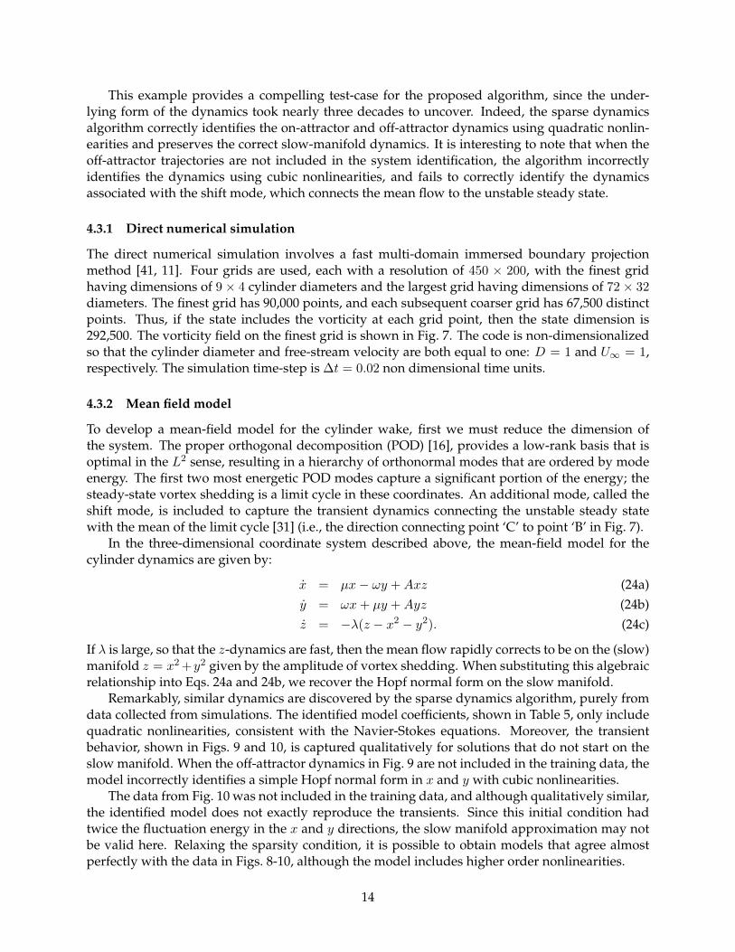
Remarkably, similar dynamics are discovered by the sparse dynamics algorithm, purely fromdata collected from simulations. The identified model coefficients, shown in Table 5, only includequadratic nonlinearities, consistent with the Navier-Stokes equations. Moreover, the transientbehavior, shown in Figs. 9 and 10, is captured qualitatively for solutions that do not start on theslow manifold. When the off-attractor dynamics in Fig. 9 are not included in the training data, themodel incorrectly identifies a simple Hopf normal form in x and y with cubic nonlinearities.

The data from Fig. 10 was not included in the training data, and although qualitatively similar,the identified model does not exactly reproduce the transients. Since this initial condition hadtwice the fluctuation energy in the x and y directions, the slow manifold approximation may notbe valid here. Relaxing the sparsity condition, it is possible to obtain models that agree almostperfectly with the data in Figs. 8-10, although the model includes higher order nonlinearities.

14

-2000

200-2000

200-150

-75

0

xy

z

Full Simulation

-2000

200-2000

200-150

-75

0

xy

z

Identified System

Figure 8: Evolution of the cylinder wake trajectory in reduced coordinates. The full simulation (left) comesfrom direct numerical simulation of the Navier-Stokes equations, and the identified system (right) capturesthe dynamics on the slow manifold. Color indicates simulation time.

-2000

200-2000

200-150

-75

0

xy

z

Full Simulation

-2000

200-2000

200-150

-75

0

xy

z

Identified System

Figure 9: Evolution of the cylinder wake trajectory starting from a flow state initialized at the mean ofthe steady-state limit cycle. Both the full simulation and sparse model capture the off-attractor dynamics,characterized by rapid attraction of the trajectory onto the slow manifold.

-2000

200-2000

200-50

0

50

xy

z

Full Simulation

-2000

200-2000

200-50

0

50

xy

z

Identified System

Figure 10: This simulation corresponds to an initial condition obtained by doubling the magnitude of thelimit cycle behavior. This data was not included in the training of the sparse model.

15

4.4 Example 4: Bifurcations and Normal Forms

It is also possible to identify normal forms associated with a bifurcation parameter µ by suspend-ing it in the dynamics as a variable:

x = f(x;µ) (25a)µ = 0. (25b)

It is then possible to identify the right hand side f(x;µ) as a sparse combination of functions ofcomponents in x as well as the bifurcation parameter µ. This idea is illustrated on two examples,the one-dimensional logistic map and the two-dimensional Hopf normal form.

4.4.1 Logistic map

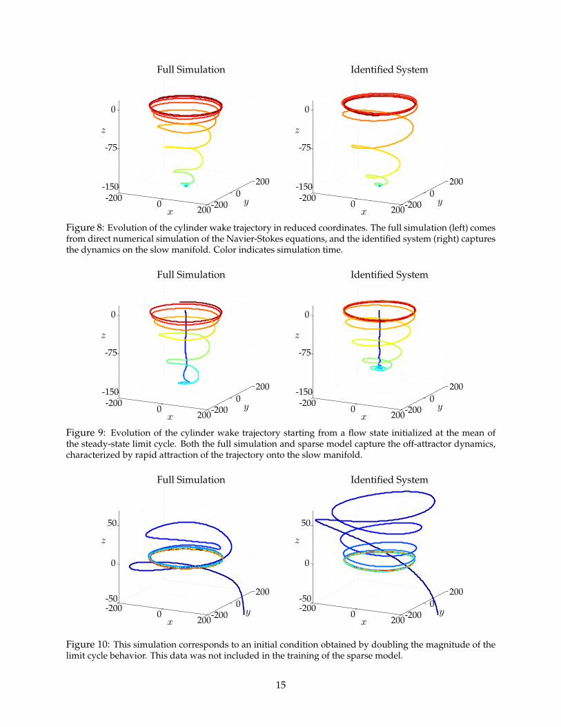
The logistic map is a classical model that exhibits a cascade of bifurcations, leading to chaotictrajectories. The dynamics with stochastic forcing ηk and parameter µ are given by

xk+1 = µxk(1− xk) + ηk. (26)

Sampling the stochastic system at ten parameter values of µ, the algorithm correctly identifies theunderlying parameterized dynamics, shown in Fig. 11 and Table 6.

Stochastic System Sparse Identified System

0 0.5 14

3

2

1

x

µ

0 0.5 14

3

2

1

x

µ

0 0.5 14

3.82

3.63

3.45

x

µ

0 0.5 14

3.82

3.63

3.45

x

µ

Figure 11: Attracting sets of the logistic map vs. the parameter µ. (left) Data from stochasticallyforced system and (right) the sparse identified system. Data is sampled at rows indicated in red forµ ∈ {2.5, 2.75, 3, 3.25, 3.5, 3.75, 3.8, 3.85, 3.9, 3.95}. The forcing ηk is Gaussian with magnitude 0.025.

16

4.4.2 Hopf normal form

The final example illustrating the ability of the sparse dynamics method to identify parameterizednormal forms is the Hopf normal form [28]. Noisy data is collected from the Hopf system

x = µx+ ωy −Ax(x2 + y2) (27a)y = −ωx+ µy −Ay(x2 + y2) (27b)

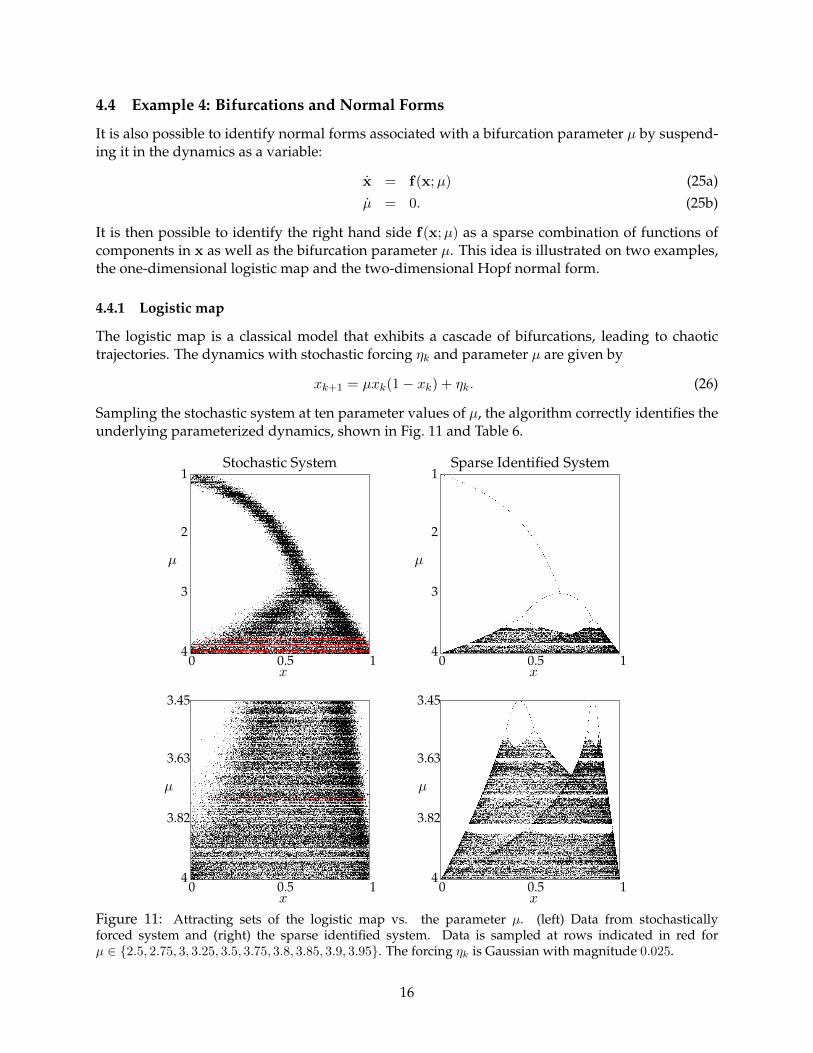
for various values of the parameter µ. Data is collected on the blue and red trajectories in Fig. 12,and noise is added to simulate sensor noise. The total variation derivative [10] is used to de-noisethe derivative for use in the algorithm.

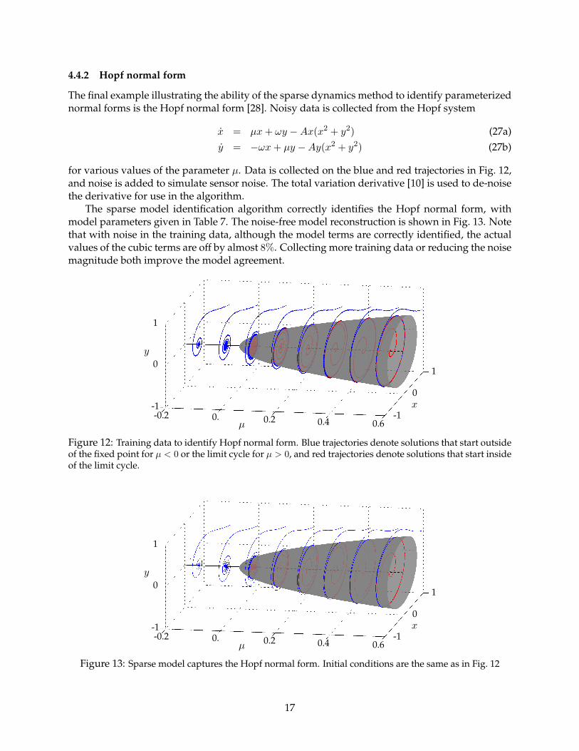
The sparse model identification algorithm correctly identifies the Hopf normal form, withmodel parameters given in Table 7. The noise-free model reconstruction is shown in Fig. 13. Notethat with noise in the training data, although the model terms are correctly identified, the actualvalues of the cubic terms are off by almost 8%. Collecting more training data or reducing the noisemagnitude both improve the model agreement.

-0.2 0. 0.2 0.4 0.6

-1

0

1

-1

0

1

µ

y

x

Figure 12: Training data to identify Hopf normal form. Blue trajectories denote solutions that start outsideof the fixed point for µ < 0 or the limit cycle for µ > 0, and red trajectories denote solutions that start insideof the limit cycle.

-0.2 0. 0.2 0.4 0.6

-1

0

1

-1

0

1

µ

y

x

Figure 13: Sparse model captures the Hopf normal form. Initial conditions are the same as in Fig. 12

17

5 Discussion

In summary, we have demonstrated a powerful new technique to identify nonlinear dynamicalsystems from data without assumptions on the form of the governing equations. This builds onprior work in symbolic regression but with innovations related to sparse regression, which al-low our algorithms to scale to high-dimensional systems. We demonstrate this new method ona number of example systems exhibiting chaos, high-dimensional data with low-rank coherence,and parameterized dynamics. As shown in the Lorenz example, the ability to predict a specifictrajectory may be less important than the ability to capture the attractor dynamics. The examplefrom fluid dynamics highlights the remarkable ability of this method to extract dynamics in afluid system that took three decades for experts in the community to explain. There are numerousfields where this method may be applied, where there is ample data and the absence of governingequations, including neuroscience, climate science, epidemiology, and financial markets. Fieldsthat already use genetic programming, such as machine learning control for turbulent fluid sys-tems [5, 34], may also benefit. Finally, normal forms may be discovered by including parametersin the optimization, as shown on two examples. The identification of sparse governing equationsand parameterizations marks a significant step toward the long-held goal of intelligent, unassistedidentification of dynamical systems.

A number of open problems remain surrounding the dynamical systems aspects of this pro-cedure. For example, many systems possess dynamical symmetries and conserved quantities thatmay alter the form of the identified dynamics. For example, the degenerate identification of alinear system in a space of high-order polynomial nonlinearities suggest a connection with near-identity transformations and dynamic similarity. We believe that this may be a fruitful line ofresearch. Finally, it will be important to identify which approximating function space to use basedon the data available. For example, it may be possible to improve the function space to make thedynamics more sparse through subsequent coordinate transformations [15].

Data science is not a panacea for all problems in science and engineering, but used in theright way, it provides a principled approach to maximally leverage the data that we have andinform what new data to collect. Big data is happening all across the sciences, where the datais inherently dynamic, and where traditional approaches are prone to overfitting. Data discoveryalgorithms that produce parsimonious models are both rare and desirable. Data-science will onlybecome more critical to efforts in science in engineering, where data is abundant, but physicallaws remain elusive. These efforts include understanding the neural basis of cognition, extractingand predicting coherent changes in the climate, stabilizing financial markets, managing the spreadof disease, and controlling turbulence,

Acknowledgements

We gratefully acknowledge valuable discussions with Bingni W. Brunton and Bernd R. Noack.SLB acknowledges support from the University of Washington department of Mechanical Engi-neering and as a Data Science Fellow in the eScience Institute (NSF, Moore-Sloan Foundation,Washington Research Foundation). JLP thanks Bill and Melinda Gates for their active support ofthe Institute for Disease Modeling and their sponsorship through the Global Good Fund. JNKacknowledges support from the U.S. Air Force Office of Scientific Research (FA9550-09-0174).

18

References[1] Zhe Bai, Thakshila Wimalajeewa, Zachary Berger, Guannan Wang, Mark Glauser, and Pramod K Varshney. Low-

dimensional approach for reconstruction of airfoil data via compressive sensing. AIAA Journal, pages 1–14, 2014.[2] R. G. Baraniuk. Compressive sensing. IEEE Signal Processing Magazine, 24(4):118–120, 2007.[3] G. Berkooz, P. Holmes, and J. L. Lumley. The proper orthogonal decomposition in the analysis of turbulent flows.

Annual Review of Fluid Mechanics, 23:539–575, 1993.[4] Josh Bongard and Hod Lipson. Automated reverse engineering of nonlinear dynamical systems. Proceedings of the

National Academy of Sciences, 104(24):9943–9948, 2007.[5] S. L. Brunton and B. R. Noack. Closed-loop turbulence control: Progress and challenges. Applied Mechanics Reviews,

67:050801–1–050801–48, 2015.[6] S. L. Brunton, J. H. Tu, I. Bright, and J. N. Kutz. Compressive sensing and low-rank libraries for classification of

bifurcation regimes in nonlinear dynamical systems. SIAM Journal on Applied Dynamical Systems, 13(4):1716–1732,2014.

[7] E. J. Candes. Compressive sensing. Proc. International Congress of Mathematics, 2006.[8] E. J. Candes, J. Romberg, and T. Tao. Robust uncertainty principles: exact signal reconstruction from highly

incomplete frequency information. IEEE Transactions on Information Theory, 52(2):489–509, 2006.[9] E. J. Candes, J. Romberg, and T. Tao. Stable signal recovery from incomplete and inaccurate measurements. Com-

munications in Pure and Applied Mathematics, 59(8):1207–1223, 2006.[10] Rick Chartrand. Numerical differentiation of noisy, nonsmooth data. ISRN Applied Mathematics, 2011, 2011.[11] T. Colonius and K. Taira. A fast immersed boundary method using a nullspace approach and multi-domain far-

field boundary conditions. Computer Methods in Applied Mechanics and Engineering, 197:2131–2146, 2008.[12] D. L. Donoho. Compressed sensing. IEEETrans.InformationTheory, 52(4):1289–1306, 2006.

[13] M. Gavish and D. L. Donoho. The optimal hard threshold for singular values is 4/√3. ArXiv e-prints, 2014.

[14] Trevor Hastie, Robert Tibshirani, Jerome Friedman, T Hastie, J Friedman, and R Tibshirani. The elements of statisticallearning, volume 2. Springer, 2009.

[15] P. Holmes and J. Guckenheimer. Nonlinearoscillations,dynamicalsystems,andbifurcations of vector fields, volume 42 ofApplied Mathematical Sciences. Springer-Verlag, Berlin, 1983.

[16] P. J. Holmes, J. L. Lumley, G. Berkooz, and C. W. Rowley. Turbulence, coherent structures, dynamical systems andsymmetry. Cambridge Monographs in Mechanics. Cambridge University Press, Cambridge, England, 2nd edition,2012.

[17] C. P. Jackson. A finite-element study of the onset of vortex shedding in flow past variously shaped bodies. Journalof Fluid Mechanics, 182:23–45, 1987.

[18] Gareth James, Daniela Witten, Trevor Hastie, and Robert Tibshirani. An introduction to statistical learning. Springer,2013.

[19] MI Jordan and TM Mitchell. Machine learning: Trends, perspectives, and prospects. Science, 349(6245):255–260,2015.

[20] I. G. Kevrekidis, C. W. Gear, J. M. Hyman, P. G. Kevrekidis, O. Runborg, and C. Theodoropoulos. Equation-free, coarse-grained multiscale computation: Enabling microscopic simulators to perform system-level analysis.Communications in Mathematical Science, 1(4):715–762, 2003.

[21] Muin J Khoury and John PA Ioannidis. Medicine. big data meets public health. Science, 346(6213):1054–1055, 2014.[22] J. R Koza. Genetic programming: on the programming of computers by means of natural selection, volume 1. MIT press,

1992.[23] L. Ljung. System Identification: Theory for the User. Prentice Hall, 1999.[24] Edward N Lorenz. Deterministic nonperiodic flow. J. Atmos. Sciences, 20(2):130–141, 1963.[25] Alan Mackey, Hayden Schaeffer, and Stanley Osher. On the compressive spectral method. Multiscale Modeling

&amp; Simulation, 12(4):1800–1827, 2014.[26] Andrew J Majda, Christian Franzke, and Daan Crommelin. Normal forms for reduced stochastic climate models.

Proceedings of the National Academy of Sciences, 106(10):3649–3653, 2009.[27] Andrew J Majda and John Harlim. Information flow between subspaces of complex dynamical systems. Proceed-

ings of the National Academy of Sciences, 104(23):9558–9563, 2007.[28] Jerrold E Marsden and Marjorie McCracken. The Hopf bifurcation and its applications, volume 19. Springer-Verlag,

1976.[29] Vivien Marx. Biology: The big challenges of big data. Nature, 498(7453):255–260, 2013.

19

[30] Igor Mezic. Analysis of fluid flows via spectral properties of the koopman operator. Annual Review of FluidMechanics, 45:357–378, 2013.

[31] B. R. Noack, K. Afanasiev, M. Morzynski, G. Tadmor, and F. Thiele. A hierarchy of low-dimensional models forthe transient and post-transient cylinder wake. Journal of Fluid Mechanics, 497:335–363, 2003.

[32] DJ Olinger and KR Sreenivasan. Nonlinear dynamics of the wake of an oscillating cylinder. Physical review letters,60(9):797, 1988.

[33] Vidvuds Ozolins, Rongjie Lai, Russel Caflisch, and Stanley Osher. Compressed modes for variational problems inmathematics and physics. Proceedings of the National Academy of Sciences, 110(46):18368–18373, 2013.

[34] V. Parezanovic, J.-C. Laurentie, T. Duriez, C. Fourment, J. Delville, J.-P. Bonnet, L. Cordier, B. R. Noack, M. Segond,M. Abel, T. Shaqarin, and S. L. Brunton. Mixing layer manipulation experiment – from periodic forcing to machinelearning closed-loop control. Journal Flow Turbulence and Combustion, 94(1):155–173, 2015.

[35] J. L. Proctor, S. L. Brunton, B. W. Brunton, and J. N. Kutz. Exploiting sparsity and equation-free architectures incomplex systems (invited review). The European Physical Journal Special Topics, 223(13):2665–2684, 2014.

[36] C. W. Rowley, I. Mezic, S. Bagheri, P. Schlatter, and D.S. Henningson. Spectral analysis of nonlinear flows. J. FluidMech., 645:115–127, 2009.

[37] D. Ruelle and F. Takens. On the nature of turbulence. Communications in Mathematical Physics, 20:167–192, 1971.[38] H. Schaeffer, R. Caflisch, C. D. Hauck, and S. Osher. Sparse dynamics for partial differential equations. Proceedings

of the National Academy of Sciences USA, 110(17):6634–6639, 2013.[39] P. J. Schmid. Dynamic mode decomposition of numerical and experimental data. Journal of Fluid Mechanics, 656:5–

28, August 2010.[40] Michael Schmidt and Hod Lipson. Distilling free-form natural laws from experimental data. Science, 324(5923):81–

85, 2009.[41] K. Taira and T. Colonius. The immersed boundary method: a projection approach. Journal of Computational Physics,

225(2):2118–2137, 2007.[42] R. Tibshirani. Regression shrinkage and selection via the lasso. J. of the Royal Statistical Society B, pages 267–288,

1996.[43] J. A. Tropp and A. C. Gilbert. Signal recovery from random measurements via orthogonal matching pursuit. IEEE

Transactions on Information Theory, 53(12):4655–4666, 2007.[44] J. Wright, A. Yang, A. Ganesh, S. Sastry, and Y. Ma. Robust face recognition via sparse representation. IEEE Trans.

on Pattern Analysis and Machine Intelligence, 31(2):210–227, 2009.[45] Z. Zebib. Stability of viscous flow past a circular cylinder. Journal of Engineering Mathematics, 21:155–165, 1987.

20

Appendix

Table 1: Damped harmonic oscillator with linear terms.

’’ ’xdot’ ’ydot’’1’ [ 0] [ 0]’x’ [-0.1015] [-1.9990]’y’ [ 2.0027] [-0.0994]’xx’ [ 0] [ 0]’xy’ [ 0] [ 0]’yy’ [ 0] [ 0]’xxx’ [ 0] [ 0]’xxy’ [ 0] [ 0]’xyy’ [ 0] [ 0]’yyy’ [ 0] [ 0]’xxxx’ [ 0] [ 0]’xxxy’ [ 0] [ 0]’xxyy’ [ 0] [ 0]’xyyy’ [ 0] [ 0]’yyyy’ [ 0] [ 0]’xxxxx’ [ 0] [ 0]’xxxxy’ [ 0] [ 0]’xxxyy’ [ 0] [ 0]’xxyyy’ [ 0] [ 0]’xyyyy’ [ 0] [ 0]’yyyyy’ [ 0] [ 0]

21

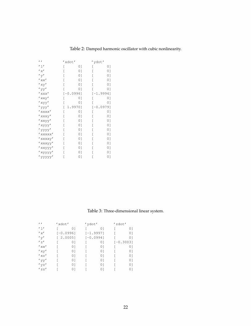
Table 2: Damped harmonic oscillator with cubic nonlinearity.

’’ ’xdot’ ’ydot’’1’ [ 0] [ 0]’x’ [ 0] [ 0]’y’ [ 0] [ 0]’xx’ [ 0] [ 0]’xy’ [ 0] [ 0]’yy’ [ 0] [ 0]’xxx’ [-0.0996] [-1.9994]’xxy’ [ 0] [ 0]’xyy’ [ 0] [ 0]’yyy’ [ 1.9970] [-0.0979]’xxxx’ [ 0] [ 0]’xxxy’ [ 0] [ 0]’xxyy’ [ 0] [ 0]’xyyy’ [ 0] [ 0]’yyyy’ [ 0] [ 0]’xxxxx’ [ 0] [ 0]’xxxxy’ [ 0] [ 0]’xxxyy’ [ 0] [ 0]’xxyyy’ [ 0] [ 0]’xyyyy’ [ 0] [ 0]’yyyyy’ [ 0] [ 0]

Table 3: Three-dimensional linear system.

’’ ’xdot’ ’ydot’ ’zdot’’1’ [ 0] [ 0] [ 0]’x’ [-0.0996] [-1.9997] [ 0]’y’ [ 2.0005] [-0.0994] [ 0]’z’ [ 0] [ 0] [-0.3003]’xx’ [ 0] [ 0] [ 0]’xy’ [ 0] [ 0] [ 0]’xz’ [ 0] [ 0] [ 0]’yy’ [ 0] [ 0] [ 0]’yz’ [ 0] [ 0] [ 0]’zz’ [ 0] [ 0] [ 0]

22

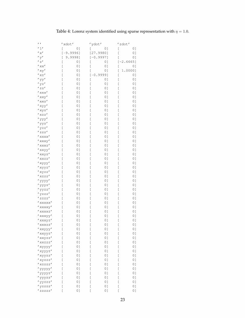
Table 4: Lorenz system identified using sparse representation with η = 1.0.

’’ ’xdot’ ’ydot’ ’zdot’’1’ [ 0] [ 0] [ 0]’x’ [-9.9996] [27.9980] [ 0]’y’ [ 9.9998] [-0.9997] [ 0]’z’ [ 0] [ 0] [-2.6665]’xx’ [ 0] [ 0] [ 0]’xy’ [ 0] [ 0] [ 1.0000]’xz’ [ 0] [-0.9999] [ 0]’yy’ [ 0] [ 0] [ 0]’yz’ [ 0] [ 0] [ 0]’zz’ [ 0] [ 0] [ 0]’xxx’ [ 0] [ 0] [ 0]’xxy’ [ 0] [ 0] [ 0]’xxz’ [ 0] [ 0] [ 0]’xyy’ [ 0] [ 0] [ 0]’xyz’ [ 0] [ 0] [ 0]’xzz’ [ 0] [ 0] [ 0]’yyy’ [ 0] [ 0] [ 0]’yyz’ [ 0] [ 0] [ 0]’yzz’ [ 0] [ 0] [ 0]’zzz’ [ 0] [ 0] [ 0]’xxxx’ [ 0] [ 0] [ 0]’xxxy’ [ 0] [ 0] [ 0]’xxxz’ [ 0] [ 0] [ 0]’xxyy’ [ 0] [ 0] [ 0]’xxyz’ [ 0] [ 0] [ 0]’xxzz’ [ 0] [ 0] [ 0]’xyyy’ [ 0] [ 0] [ 0]’xyyz’ [ 0] [ 0] [ 0]’xyzz’ [ 0] [ 0] [ 0]’xzzz’ [ 0] [ 0] [ 0]’yyyy’ [ 0] [ 0] [ 0]’yyyz’ [ 0] [ 0] [ 0]’yyzz’ [ 0] [ 0] [ 0]’yzzz’ [ 0] [ 0] [ 0]’zzzz’ [ 0] [ 0] [ 0]’xxxxx’ [ 0] [ 0] [ 0]’xxxxy’ [ 0] [ 0] [ 0]’xxxxz’ [ 0] [ 0] [ 0]’xxxyy’ [ 0] [ 0] [ 0]’xxxyz’ [ 0] [ 0] [ 0]’xxxzz’ [ 0] [ 0] [ 0]’xxyyy’ [ 0] [ 0] [ 0]’xxyyz’ [ 0] [ 0] [ 0]’xxyzz’ [ 0] [ 0] [ 0]’xxzzz’ [ 0] [ 0] [ 0]’xyyyy’ [ 0] [ 0] [ 0]’xyyyz’ [ 0] [ 0] [ 0]’xyyzz’ [ 0] [ 0] [ 0]’xyzzz’ [ 0] [ 0] [ 0]’xzzzz’ [ 0] [ 0] [ 0]’yyyyy’ [ 0] [ 0] [ 0]’yyyyz’ [ 0] [ 0] [ 0]’yyyzz’ [ 0] [ 0] [ 0]’yyzzz’ [ 0] [ 0] [ 0]’yzzzz’ [ 0] [ 0] [ 0]’zzzzz’ [ 0] [ 0] [ 0]

23

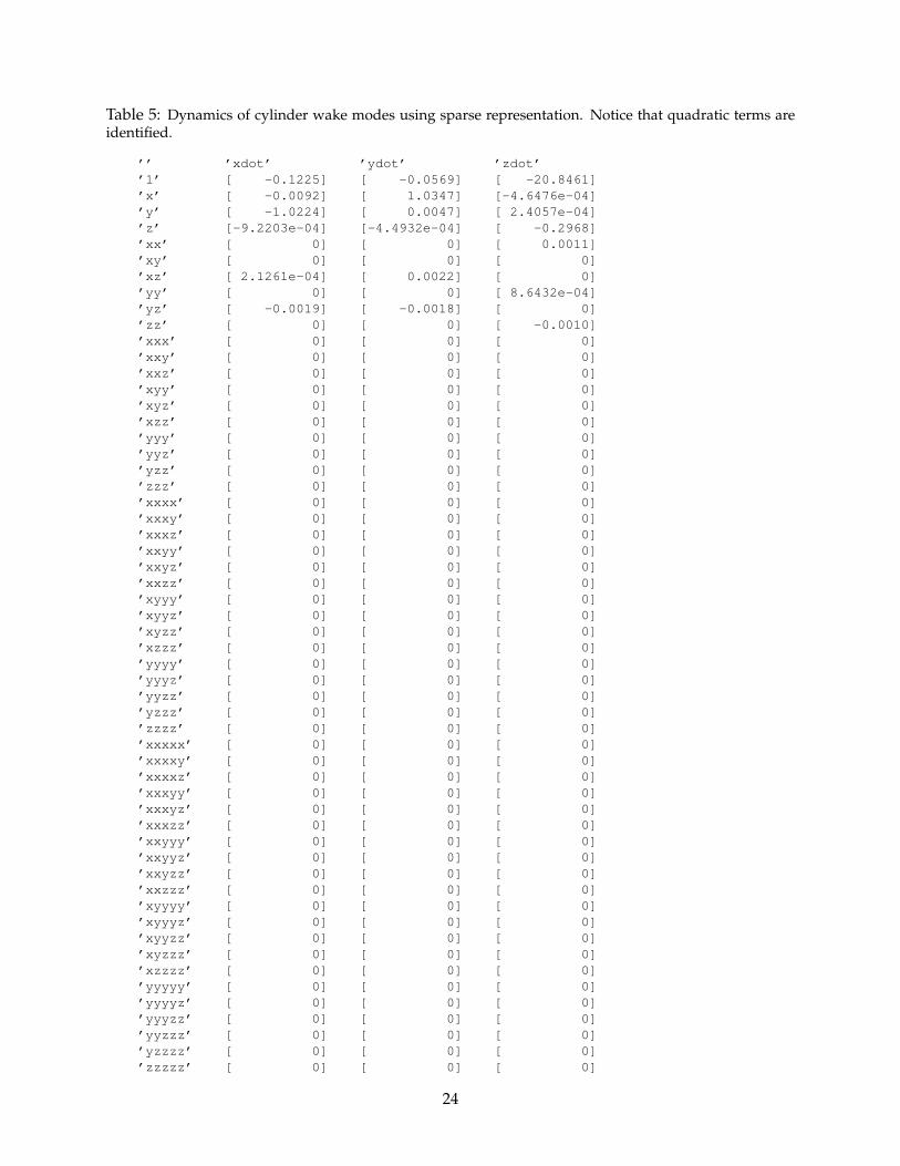
Table 5: Dynamics of cylinder wake modes using sparse representation. Notice that quadratic terms areidentified.

’’ ’xdot’ ’ydot’ ’zdot’’1’ [ -0.1225] [ -0.0569] [ -20.8461]’x’ [ -0.0092] [ 1.0347] [-4.6476e-04]’y’ [ -1.0224] [ 0.0047] [ 2.4057e-04]’z’ [-9.2203e-04] [-4.4932e-04] [ -0.2968]’xx’ [ 0] [ 0] [ 0.0011]’xy’ [ 0] [ 0] [ 0]’xz’ [ 2.1261e-04] [ 0.0022] [ 0]’yy’ [ 0] [ 0] [ 8.6432e-04]’yz’ [ -0.0019] [ -0.0018] [ 0]’zz’ [ 0] [ 0] [ -0.0010]’xxx’ [ 0] [ 0] [ 0]’xxy’ [ 0] [ 0] [ 0]’xxz’ [ 0] [ 0] [ 0]’xyy’ [ 0] [ 0] [ 0]’xyz’ [ 0] [ 0] [ 0]’xzz’ [ 0] [ 0] [ 0]’yyy’ [ 0] [ 0] [ 0]’yyz’ [ 0] [ 0] [ 0]’yzz’ [ 0] [ 0] [ 0]’zzz’ [ 0] [ 0] [ 0]’xxxx’ [ 0] [ 0] [ 0]’xxxy’ [ 0] [ 0] [ 0]’xxxz’ [ 0] [ 0] [ 0]’xxyy’ [ 0] [ 0] [ 0]’xxyz’ [ 0] [ 0] [ 0]’xxzz’ [ 0] [ 0] [ 0]’xyyy’ [ 0] [ 0] [ 0]’xyyz’ [ 0] [ 0] [ 0]’xyzz’ [ 0] [ 0] [ 0]’xzzz’ [ 0] [ 0] [ 0]’yyyy’ [ 0] [ 0] [ 0]’yyyz’ [ 0] [ 0] [ 0]’yyzz’ [ 0] [ 0] [ 0]’yzzz’ [ 0] [ 0] [ 0]’zzzz’ [ 0] [ 0] [ 0]’xxxxx’ [ 0] [ 0] [ 0]’xxxxy’ [ 0] [ 0] [ 0]’xxxxz’ [ 0] [ 0] [ 0]’xxxyy’ [ 0] [ 0] [ 0]’xxxyz’ [ 0] [ 0] [ 0]’xxxzz’ [ 0] [ 0] [ 0]’xxyyy’ [ 0] [ 0] [ 0]’xxyyz’ [ 0] [ 0] [ 0]’xxyzz’ [ 0] [ 0] [ 0]’xxzzz’ [ 0] [ 0] [ 0]’xyyyy’ [ 0] [ 0] [ 0]’xyyyz’ [ 0] [ 0] [ 0]’xyyzz’ [ 0] [ 0] [ 0]’xyzzz’ [ 0] [ 0] [ 0]’xzzzz’ [ 0] [ 0] [ 0]’yyyyy’ [ 0] [ 0] [ 0]’yyyyz’ [ 0] [ 0] [ 0]’yyyzz’ [ 0] [ 0] [ 0]’yyzzz’ [ 0] [ 0] [ 0]’yzzzz’ [ 0] [ 0] [ 0]’zzzzz’ [ 0] [ 0] [ 0]

24

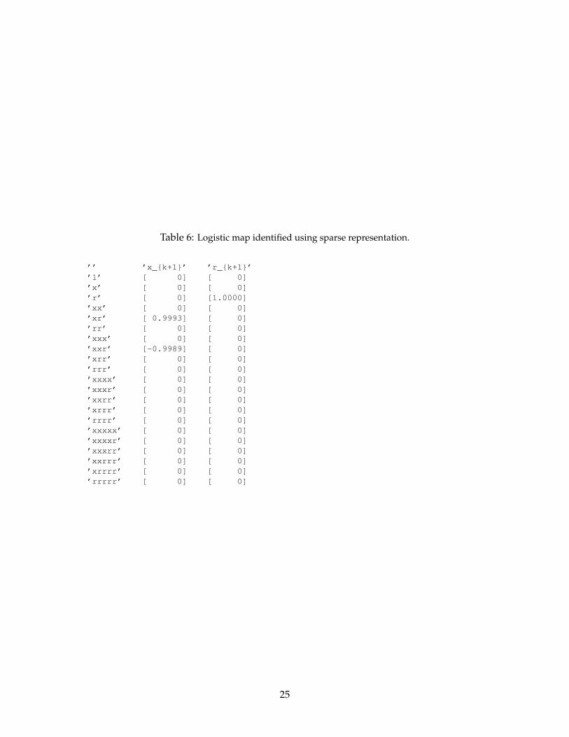
Table 6: Logistic map identified using sparse representation.

’’ ’x_{k+1}’ ’r_{k+1}’’1’ [ 0] [ 0]’x’ [ 0] [ 0]’r’ [ 0] [1.0000]’xx’ [ 0] [ 0]’xr’ [ 0.9993] [ 0]’rr’ [ 0] [ 0]’xxx’ [ 0] [ 0]’xxr’ [-0.9989] [ 0]’xrr’ [ 0] [ 0]’rrr’ [ 0] [ 0]’xxxx’ [ 0] [ 0]’xxxr’ [ 0] [ 0]’xxrr’ [ 0] [ 0]’xrrr’ [ 0] [ 0]’rrrr’ [ 0] [ 0]’xxxxx’ [ 0] [ 0]’xxxxr’ [ 0] [ 0]’xxxrr’ [ 0] [ 0]’xxrrr’ [ 0] [ 0]’xrrrr’ [ 0] [ 0]’rrrrr’ [ 0] [ 0]

25

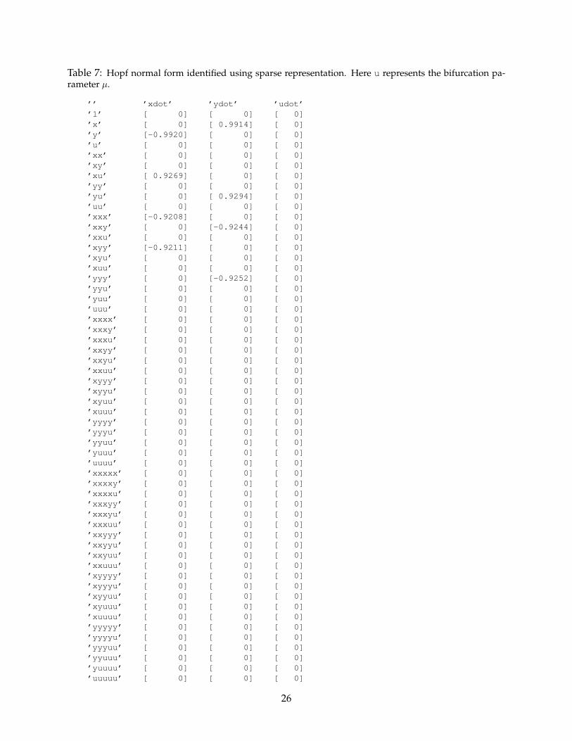
Table 7: Hopf normal form identified using sparse representation. Here u represents the bifurcation pa-rameter µ.

’’ ’xdot’ ’ydot’ ’udot’’1’ [ 0] [ 0] [ 0]’x’ [ 0] [ 0.9914] [ 0]’y’ [-0.9920] [ 0] [ 0]’u’ [ 0] [ 0] [ 0]’xx’ [ 0] [ 0] [ 0]’xy’ [ 0] [ 0] [ 0]’xu’ [ 0.9269] [ 0] [ 0]’yy’ [ 0] [ 0] [ 0]’yu’ [ 0] [ 0.9294] [ 0]’uu’ [ 0] [ 0] [ 0]’xxx’ [-0.9208] [ 0] [ 0]’xxy’ [ 0] [-0.9244] [ 0]’xxu’ [ 0] [ 0] [ 0]’xyy’ [-0.9211] [ 0] [ 0]’xyu’ [ 0] [ 0] [ 0]’xuu’ [ 0] [ 0] [ 0]’yyy’ [ 0] [-0.9252] [ 0]’yyu’ [ 0] [ 0] [ 0]’yuu’ [ 0] [ 0] [ 0]’uuu’ [ 0] [ 0] [ 0]’xxxx’ [ 0] [ 0] [ 0]’xxxy’ [ 0] [ 0] [ 0]’xxxu’ [ 0] [ 0] [ 0]’xxyy’ [ 0] [ 0] [ 0]’xxyu’ [ 0] [ 0] [ 0]’xxuu’ [ 0] [ 0] [ 0]’xyyy’ [ 0] [ 0] [ 0]’xyyu’ [ 0] [ 0] [ 0]’xyuu’ [ 0] [ 0] [ 0]’xuuu’ [ 0] [ 0] [ 0]’yyyy’ [ 0] [ 0] [ 0]’yyyu’ [ 0] [ 0] [ 0]’yyuu’ [ 0] [ 0] [ 0]’yuuu’ [ 0] [ 0] [ 0]’uuuu’ [ 0] [ 0] [ 0]’xxxxx’ [ 0] [ 0] [ 0]’xxxxy’ [ 0] [ 0] [ 0]’xxxxu’ [ 0] [ 0] [ 0]’xxxyy’ [ 0] [ 0] [ 0]’xxxyu’ [ 0] [ 0] [ 0]’xxxuu’ [ 0] [ 0] [ 0]’xxyyy’ [ 0] [ 0] [ 0]’xxyyu’ [ 0] [ 0] [ 0]’xxyuu’ [ 0] [ 0] [ 0]’xxuuu’ [ 0] [ 0] [ 0]’xyyyy’ [ 0] [ 0] [ 0]’xyyyu’ [ 0] [ 0] [ 0]’xyyuu’ [ 0] [ 0] [ 0]’xyuuu’ [ 0] [ 0] [ 0]’xuuuu’ [ 0] [ 0] [ 0]’yyyyy’ [ 0] [ 0] [ 0]’yyyyu’ [ 0] [ 0] [ 0]’yyyuu’ [ 0] [ 0] [ 0]’yyuuu’ [ 0] [ 0] [ 0]’yuuuu’ [ 0] [ 0] [ 0]’uuuuu’ [ 0] [ 0] [ 0]

26