1

Discovering Equations that Govern Experimental Materials Stability under Environmental Stress using Scientific Machine Learning

Richa Ramesh Naik*, Armi Tiihonen*, Janak Thapa, Clio Batali, Zhe Liu, Shijing Sun, Tonio Buonassisi*

Massachusetts Institute of Technology, 77 Massachusetts Avenue, Cambridge, MA 02139

*Correspondence to: RN (richarnaik96@gmail.com), AT (armi.tiihonen@gmail.com), TB (buonassisi@mit.edu)

June 21, 2021 version

Abstract:

While machine learning (ML) in experimental research has demonstrated impressive predictive

capabilities, inductive reasoning and knowledge extraction remain elusive tasks, in part because

of the difficulty extracting fungible knowledge representations from experimental data. In this

manuscript, we use ML to infer the underlying dynamical differential equation (DE) from

experimental data of degrading organic-inorganic methylammonium lead iodide (MAPI)

perovskite thin films under environmental stressors (elevated temperature, humidity, and light).

We apply a sparse regression algorithm that automatically identifies the differential equation

describing the dynamics from time-series data. We find that the underlying DE governing MAPI

degradation across a broad temperature range of 35 to 85°C is described minimally with three

terms (specifically, a second-order polynomial), and not a simple single-order reaction (i.e. 0th, 1st,

or 2nd-order reaction). We demonstrate how computer-derived results can aid the researcher to

develop profound mechanistic insights. This DE corresponds to the Verhulst logistic function,

which describes reaction kinetics analogous in functional form to autocatalytic or self-propagating

reactions, suggesting future strategies to suppress MAPI degradation. We examine the robustness

of our conclusions to experimental luck-of-the-draw variance and Gaussian noise using a

combination of experiment and simulation, and describe the experimental limits within which this

methodology can be applied. Our study demonstrates the application of scientific ML in

experimental chemical and materials systems, highlighting the promise and challenges associated

with ML-aided scientific discovery.

2

Introduction

In the traditional scientific discovery process, prior knowledge from first-principles and empirical

laws are combined with experimental data and intuition to yield governing equations. Newton’s

law of gravitation1, Einstein’s mass-energy equivalence equation2, Kepler’s laws of planetary

motion3 and other physical principles were uncovered through careful interpretation of

experimental data and inductive reasoning4. The approach of fitting experimental data through

regression is difficult with systems that are yet to be understood fully – the set of feasible equations

capturing the physics is enormous.5–7

One such area where underlying physics is often poorly understood is the study of materials under

environmental stress. For example, alloys8,9, polymers10, doped silicon11 and hybrid materials12

experience changes at elevated temperatures. The degradation pathways can be complex and not

directly obvious when examining the experimental data. Machine learning (ML) has been used to

predict degradation13–17 as well as to optimize process conditions to reduce material

decomposition16,18. However, traditional data-science methods yield little insight into the

underlying mechanisms. We posit that hidden in the black-box ML models is valuable scientific

information on the dynamics of the system. If uncovered, the knowledge of the governing

dynamics can serve as foundation for physical interpretation of phenomena and scientific

discovery.

Herein, we use scientific ML, which combines regression-based ML with sparsity generating

techniques in order to automatically identify governing equations directly from data, especially

when the systems being studied are too complicated to yield to traditional theoretical analysis. Not

only does scientific ML help us understand the underlying scientific phenomena better, it also has

the potential to help to make simulations faster and extrapolate beyond the dataset at hand.

Recently, many approaches aiming for this target have been presented in literature. A method that

we apply in this contribution is PDE-FIND by Rudy et al.19 This method is used for the discovery

of physical laws describing dynamical systems. First, a library of potential candidate functions is

built. Differentials are calculated by finite difference or polynomial interpolation. Once a large

matrix with all candidate functions is composed, different sparse regression methods may be used

to extract the partial differential equation (PDE) describing the system. The sparse methods

implemented are sequential threshold ridge regression, lasso regression, elastic net regression and

3

greedy algorithm. Another sparse technique is Sparse Identification of nonlinear Dynamics

(SINDy)20. It uses a custom deep autoencoder to find a coordinate system in which the dynamics

of the system are sparse, and then uses sparse regression to find the governing equations in the

associated coordinate system. Atkinson et al.21 present a generalized method for the discovery of

differential equations using genetic programming. Physics Informed Neural Networks (PINN) 22

and PDE-NET23,24 are deep learning methodologies to extract governing partial differential

equations using dynamical data. These methods have shown great promise in several

applications25–28. The automatic discovery of scientific laws and principles is at the frontier of

machine learning that awaits application to materials science29 and other domains30–32.

Halide perovskite materials, which have potential to provide high performing and cost-effective

solar energy, degrade at elevated temperature33–38, humidity39–41, and illumination42,43. This is a

major issue hindering the commercialization of perovskite photovoltaic technology. However, the

degradation mechanisms affecting halide perovskites are not well understood. Discovering the

underlying equations directly from perovskite degradation data could accelerate the development

of stable perovskite solar cells. Herein, we apply Scientific ML to study the environmental

degradation of methylammonium lead iodide (MAPI).

From prior knowledge in the literature, MAPI has multiple documented reaction pathways,

including decomposition to PbI2 via reaction44:

𝑀𝐴𝑃𝑏𝐼! → 𝑃𝑏𝐼" + [𝐶𝐻!𝑁𝐻!# + 𝐼$] → 𝑃𝑏𝐼" + 𝐶𝐻!𝑁𝐻" + 𝐻𝐼 (1)

Smecca et al.45 demonstrate that the rate of MAPI degradation obeys an Arrhenius-type law. Their

data suggests that the degradation of MAPI follows zero-order kinetics in the presence of moisture

and first-order kinetics in vacuum at temperatures ranging from 90℃ to 135℃. Bastos et al.46

hypothesize that the thermal degradation of MAPI is defined by the Avrami equation47,48 of

nucleation and growth. The Avrami equation has also been used to describe degradation kinetics

in humid air49. Recently, studies have shown that halide perovskite degradation follows

autocatalytic reaction kinetics50 with the hypothesis that the degradation is propagated by iodine

vapors51. The derivation of exact kinetics through first principles as well as Arrhenius-type

dependence is difficult because of the complexity of MAPI decomposition, despite the availability

of well-resolved dynamical data, inviting the application of Scientific ML.

4

In this study, we focus on the application of PDE-FIND to perovskite degradation data. We choose

PDE-FIND as it is an interpretable method that provides a parsimonious description of the

dynamics with the flexibility to apply domain expertise for library selection. Successfully

identifying governing differential equations directly from the experimental aging test data would

deepen the understanding of thermal degradation and provide tools for reliable lifetime prediction

of perovskite solar cells as well as the determination of acceleration factors for long-term aging

tests. These developments could spur the advancement of the perovskite photovoltaic technology

and have been called for by the community52–54. This study provides a generalizable pathway to

identify degradation modes in other materials research domains as well.

5

Methods

Figure 1. Schematic of the data-management workflow used in this study. Workflow (1) applies

PDE-FIND directly to experimental data; Workflow (2) first fits the experimental data with a

logistic function to create a simulated dataset, optionally adds Gaussian noise, and then applies

PDE-FIND.

A summary of our data-analysis workflow is shown in Figure 1. Our goals for this study are two-

fold: Uncover the underlying differential equation corresponding to perovskite degradation using

sparse regression methodology PDE-FIND (Workflow (1)) and quantify the effect of noise on the

accuracy of extraction of differential equations by PDE-FIND by comparing noiseless and noisy

simulated data (Workflow (2)). This is represented by the two workflows in Figure 1.

For the first objective, the input is the experimental data obtained from degrading MAPI films.

Our experimental data is shown in Figure 2. We subjected 206 thin-film samples of

methylammonium lead iodide (MAPI) to 0.15±0.01 Sun illumination, 20±5% relative humidity,

and temperatures varying from 35 to 85°C in our in-house environmental chamber described in

detail in Ref. 18 (Figure 2b). One hundred and eight samples were grown under low-variance

conditions (labeled “low-variance experimental”); ninety-eight samples were grown under high-

variance conditions (labeled “high-variance experimental”) (Figure S2). Unless specified

6

otherwise, we assume “experimental” data in this paper refers to the low-variance sample set. We

quantify this variance in the beginning of the “Results” section.

We monitored the degradation of MAPI based on the color change of the material. As MAPI films

decompose, they change their color from initial black (majority MAPI) to degraded yellow

(minority MAPI). We acquired images of the degrading films with 0.5-minute temporal resolution

and processed them to obtain the average red, blue and green color components of the films as a

function of time (Figure 2a, Figure S1). The red color time-series is chosen for further analysis

because it sufficiently captures the temporal perovskite decomposition behavior at the MAPI

bandgap, as shown in the Supporting Information of Ref. 16 (Figure 2d, Figure S1).

Figure 2. The experimental data. a) Average perovskite film color as a function of time at different

temperatures. b) A schematic diagram of the in-house accelerated degradation chamber with a

superimposed camera image of degrading MAPI films. c) The structure of MAPI perovskite

(reactant) and lead iodide (degradation product). d) Processed average red color component of

films degraded at T = 55 °C as a function of time.

For the second objective, we generate simulated degradation data to analyze how noise obfuscates

the identification of underlying DEs. We apply a non-linear least-squares method to fit the

7

experimental data (e.g., those shown in Figure 2d) to the Verhulst logistic equation55 to model the

S-shaped curve. This is a reasonable assumption because the logistic function is used to describe

the thermal decomposition dynamics of several materials50,51,56.We obtain,

𝑈 = 𝑀 +𝑈%𝐾𝑒&'

(𝐾 − 𝑈%) + 𝑈%𝑒&', (2)

𝜕𝑈𝜕𝑡 = 𝑘(𝑈 −𝑀):1 −

(𝑈 −𝑀)𝐾 ; (3)

where Uo is the initial concentration, k is growth rate, K is the carrying capacity and M is a fitting

constant. In the context of MAPI degradation, M, Uo and K can be considered as fitting parameters.

The growth rate k varies with temperature according to the Arrhenius equation:

𝑘 = 𝐴𝑒!−𝐸a𝑅𝑇" (4)

Here, Ea is the activation energy, T is the temperature in Kelvin, A is the pre-exponential factor

and R is the universal gas constant. We use this model to produce noise-free simulated data (labeled

“simulated”) and simulated data with Gaussian noise (labelled “simulated with Gaussian noise”).

First, we apply the sparse regression methodology PDE-FIND19 to experimental data (Workflow

(1)). We use the time-series from all the temperatures to infer the partial differential equation

(PDE) defining the relationship between MAPI degradation, temperature and time. Then, we apply

PDE-FIND to the time-dependent degradation data at each temperature, to infer the ordinary

differential equation (ODE) that describes MAPI decomposition at a particular temperature. To

study the effect of noise, we apply PDE-FIND to simulated data with and without Gaussian noise

(Workflow (2)).

The library of potential candidate functions consists of polynomials of U, polynomials of time t, sine and cosine of U, Temperature T and other non-linear functions of U, tand T(TableS1). Differentials are calculated by finite difference with convolutional smoothing using a 1D Gaussian

kernel. Once a large tall matrix (Θ(U)) with all candidate functions is composed, we use sequential

threshold ridge regression to identify which terms contribute to the dynamics described by the data

as well as those terms’ weights. The goal of this method is to find a sparse coefficient vector β that

only consists of the active features that best represent the time derivative 𝑈' . The rest of the

8

features are hard-thresholded to zero. The loss functions are follows (λ2 and λ0 are the L-2 and L-

0 regularization penalties respectively, more details can be found in in the supplementary

information of Ref. 19):

𝛽H = argmin,(‖𝛩(𝑈)𝛽 − 𝑈'‖" + 𝜆"‖𝛽‖") (5.1)

for a given tolT , where tolT is:

tolT = argmin-%.(‖𝛩(𝑈)𝛽 − 𝑈'‖" + 𝜆/‖𝛽‖/) (5.2)

9

Results

Our aim is to obtain the equation that most accurately describes the environmental degradation of

methylammonium lead iodide (MAPI) as a function of time and temperature. There are two main

challenges for scientific ML in this application that are also common with many other experimental

applications, especially in materials science: The function space that could in principle capture the

degradation processes is enormous, complicating identification of unique equations. Furthermore,

experimental data has measurement noise as well as sample-to-sample variance, making the

identification of quantitative analytic descriptions even more challenging. These conditions can be

optimized to some extent, but not excluded.

Our experimental setup represents a typical materials science experiment: The noise in our

experimental data is of the order of 0.35% for both high-variance and low-variance experimental

data sets. The low value indicates that the camera measurement of degradation is optimized. The

sample-to-sample variance for the “low variance experimental” dataset is estimated to be 20% in

relative standard deviation and the maximum mean absolute deviation is 12 units (Red color value

varies from 0-255). For the “high variance experimental” dataset, variance is estimated to be 23%

in relative standard deviation and the maximum mean absolute deviation is 31 units. These values

are typical for spin-coated perovskite film samples that tend to have rather high variations,

especially when aged.

Our workflow shown in Figure 2. First, we attempt to uncover the differential equation governing

perovskite degradation directly from experimental data (Workflow (1)). A simple way to analyze

reaction rate orders is to fit the data to pure 0th, 1st and 2nd order dynamics (Figure S3). These

equations do not fit the data, showing that the environmental degradation of MAPI does not follow

a simple n-th order kinetics. This motivates the use of PDE-FIND. We apply sparse regression to

the whole experimental dataset with a broad function library consisting of polynomials of U up to

order 5, sine and cosine of U, polynomials of t up to order 3, the square root of t, U multiplied with

polynomials of t, temperature T and adjusted negative exponent of 1/T (exp(− 0//1)). Sine and

cosine terms are not selected by PDE-FIND –indicating as a sanity check that the algorithm

correctly identifies that periodicity is not a feature of the dynamics. Polynomials of t and U times

the polynomials of t, which correspond to the Avrami equation, are not included in the library or

assigned very small weights. To understand how well the obtained DE represents our data, we

10

compare the derivative estimated by our DE to the numerical derivative obtained from the

experimental data. While certain trends in the derivative are captured, errors exist because of the

variance in our experimental data (Figure S4). Refinements to the approach are thus needed.

We proceed to narrow the application of PDE-FIND, by applying PDE-FIND to the averaged data

at each temperature individually to extract the governing ODE. Using the averaged data helps us

deal with sample-to-sample variance. Since all environmental conditions were almost identical for

samples degraded at a particular temperature but aging tests of each temperature were conducted

one after another (introducing differences e.g. in sample storage times and exact equipment

atmosphere), we aim to reduce the influence of variance-inducing conditions by applying PDE-

FIND at each temperature separately. First, we apply PDE-FIND with a large library as described

in the previous paragraph. Here too, we see that sine and cosine of U, polynomials of t and U times

the polynomials of t are either removed from the library or have small coefficient values. We

exclude these terms in further analysis. Then, we apply PDE-FIND with 1st to 5th order polynomial

libraries. We find that with the 1st order polynomial library, PDE-FIND is unable to find an

equation that fits the derivative of our data (Figure 3a). All other libraries from 2nd order

polynomial to 5th order polynomial appear to fit the derivative of our data with significant accuracy

(Figure 3a, 3b). When these differential equations are integrated, they have the same S-shape as

our experimental data (Figure 3c). The 2nd order polynomial library is the most minimal library

that fits our data without high error. The functional form of this ODE is:

𝑑𝑈𝑑𝑡 = 𝑎# + 𝑎$𝑈 + 𝑎%𝑈% (6)

We also notice a trend in the values of the fitting coefficients with respect to temperature –

especially in the case of the 2nd order polynomial library (Figure 3d, Figure S5). Then slope of the

curve changes between 55 °C and 65 °C, the temperature at which a well-known MAPI phase

transition57,58 occurs. This may indicate that the phase transition affects the degradation

mechanism, but is not experimentally confirmed in this work.

11

Figure 3. PDE-FIND results with experimental data: a) A bar plot shows the MAE between the

actual experimental derivative (smoothened) and the value of the derivative estimated using the

differential equation identified by PDE-FIND. Inset: Comparison of the experimental data with

the curve obtained by integrating the equation identified by PDE-FIND with 2nd order polynomial

library . b) Comparison of the dU/dt calculated from experimental data for T = 55 °C and estimated

from PDE-FIND for 2nd order polynomial library to 5th order polynomial libraries c) Coefficient

values estimated by PDE-FIND as a function of temperature for 2nd order polynomial library.

Next, we evaluate the effect of variance on PDE extraction by comparing the above results

(obtained on the low-variance experimental dataset) with the same workflow applied to the high-

variance data (Figure S6). After averaging multiple curves (U(t)) for each temperature, the results

are qualitatively similar for a constrained function library of polynomials of 2nd order – the

obtained coefficients have the same sign and order of magnitude. This indicates that PDE-FIND

can fit even high-variance experimental data when appropriately averaging over multiple samples.

To quantify the effect of sample-to-sample variance, we apply PDE-FIND to each curve

individually. As expected, PDE-FIND extracts a large variance in coefficient values. The values

12

of coefficients vary as much as 60% with the low variance dataset and up to 90% with the high

variance datasets for T = 55 °C.

Now, we evaluate the effect of noise on PDE extraction using simulated data. We use the non-

linear least-squares method to fit our experimental data to the Verhulst logistic equation55 and the

Arrhenius equation, as shown in the Methods section. We produce both noise-free simulated data

and simulated data with Gaussian noise (Workflow (2)) with this model.

We apply sparse regression to the simulated dataset at each temperature individually to discover

the governing ODEs with libraries ranging from 2nd to 5th order polynomials. With the noise-free

data, PDE-FIND’s identified DEs fit the derivative as well as the data on integration of the DE

with significant accuracy for libraries from 2nd order to 5th order. In the case of the 2nd order

polynomial library, both the underlying differential equation and the fitting parameters are

identified with significant accuracy, as shown in Figure 4. We know that the underlying governing

equation for this dataset should have terms of orders higher than 2 equals to zero – PDE-FIND

assigns small non-zero values to these functional forms, although they are not set to zero. In the

case where sine and cosine are added to the library, the algorithm correctly identifies that these

terms do not represent the dynamics and are set to zero exactly. The MAE between the exact

numerical derivative and one estimated from the differential equation identified by PDE-FIND is

of order 10-7 (when derivative varies from 0 to 1). This indicates that PDE-FIND works well for

simulated curves with zero noise. Thus, with the candidate function library constrained to

polynomials of U, PDE-FIND is able to identify the same ODE that fits the data at each

temperature.

We then add varying amounts of Gaussian noise to this simulated equation at different

temperatures. First, we consider the effect of varying amounts of noise at a fixed temperature of

55°C, as indicated by the black box in Figure 4a. We add up to 5% noise, which is typical in many

experimental settings. The equation identified by PDE-FIND yields an S-shaped curve similar to

the noise-free simulated curve upon integration (Figure 4d) for up to 5% noise, after which the DE

identified by PDE-FIND doesn’t seem to model the dynamics. We compare the error of estimating

the parameter values in the differential equation describing the simulated data. At 5% Gaussian

noise the error of the fitting parameters increases to almost 80% (Figure 4b). The resulting

integrated curve has MAE as low as 6 (on a color scale of 0-255) relative to the “ground truth”

13

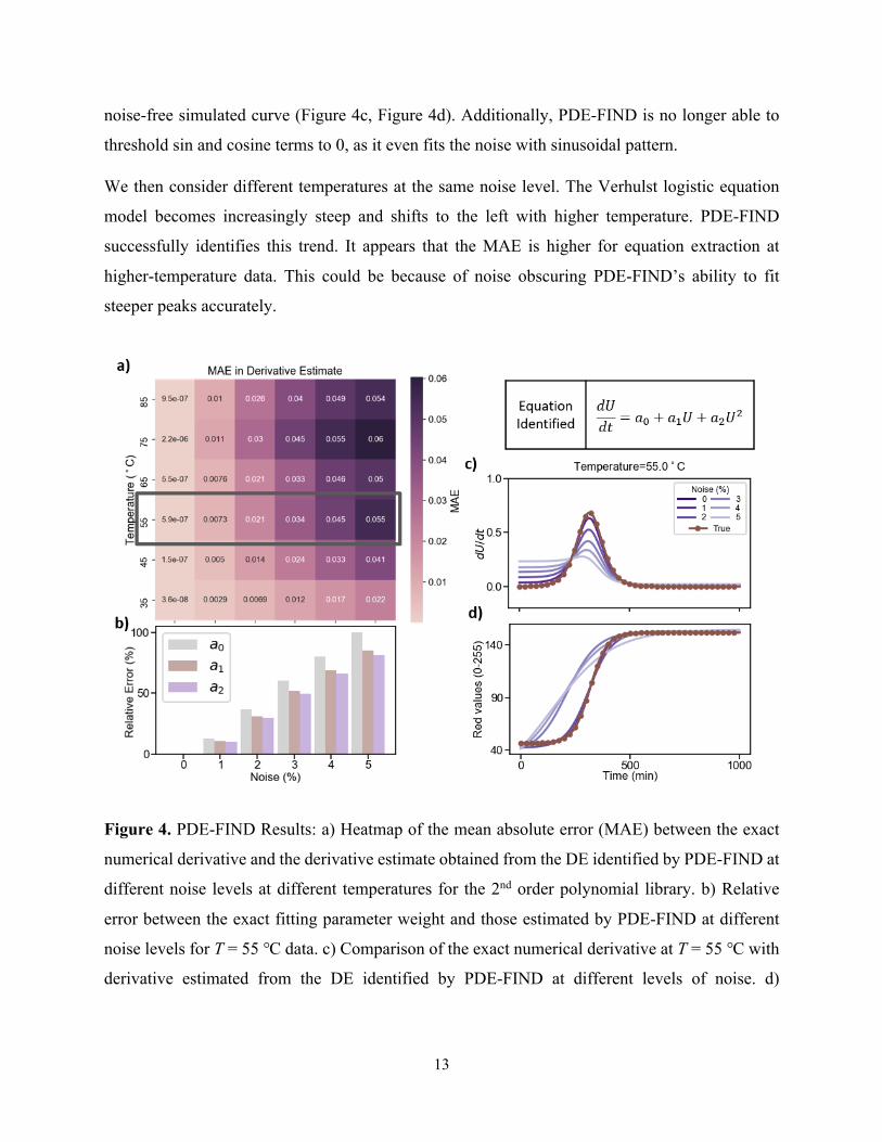
noise-free simulated curve (Figure 4c, Figure 4d). Additionally, PDE-FIND is no longer able to

threshold sin and cosine terms to 0, as it even fits the noise with sinusoidal pattern.

We then consider different temperatures at the same noise level. The Verhulst logistic equation

model becomes increasingly steep and shifts to the left with higher temperature. PDE-FIND

successfully identifies this trend. It appears that the MAE is higher for equation extraction at

higher-temperature data. This could be because of noise obscuring PDE-FIND’s ability to fit

steeper peaks accurately.

Figure 4. PDE-FIND Results: a) Heatmap of the mean absolute error (MAE) between the exact

numerical derivative and the derivative estimate obtained from the DE identified by PDE-FIND at

different noise levels at different temperatures for the 2nd order polynomial library. b) Relative

error between the exact fitting parameter weight and those estimated by PDE-FIND at different

noise levels for T = 55 ℃ data. c) Comparison of the exact numerical derivative at T = 55 ℃ with

derivative estimated from the DE identified by PDE-FIND at different levels of noise. d)

14

Comparison of the exact solution at T = 55 ℃ with solution curves obtained by integrating the DE

identified by PDE-FIND at different levels of noise.

15

Discussion

There remain many complex systems that have eluded quantitative analytic descriptions or even

characterization of a suitable choice of variables in many disciplines such as biology, finance and

materials science. With today's state-of-the art equipment, acquiring large quantities of data has

never been easier. As put by Rackauckas et al.59, “the well-known adage ‘a picture is worth a

thousand words' might well be 'a model is worth a thousand datasets.’”.

i. Scientific ML enables unique insights into MAPI degradation

Scientific ML is a promising method that can be used to uncover governing equations through

data, especially when the derivation of physical laws using first principles is challenging. In our

study, we demonstrate that PDE-FIND identifies an underlying rate equation for the degradation

of perovskite solar cells. MAPI degradation does not follow a simple single-order reaction rate

law, defined as:

𝑑𝑈𝑑𝑡

= 𝑘𝑈2 (7)

where, n is the order of the reaction and U is the concentration of the species. In our system, this

equation does not yield a good fit for n=0, 1 or 2. The S-shaped dynamics we see in our study have

been reported in other studies involving MAPI degradation as well 46,49–51. Some articles report

that the degradation results from nucleation and growth of PbI2 crystals46,49, supporting the

hypothesis that the kinetics follows the Johnson-Mehl-Avrami-Kolmorgorov or simply, the

Avrami equation47,48:

𝑑𝑈3

𝑑𝑡 = 𝑎/𝑡2$0 − 𝑎0𝑈3𝑡2$0 (8)

𝑈3(') = 1 − exp(−𝑘𝑡2) (9)

Where,

𝑈3(𝑡) =𝑈(𝑡) − min(𝑈)

max(𝑈 − min(𝑈))

And a0, a1, n and k are fitting constants.

16

Some recent studies have presented an alternate hypothesis of self-propagating or autocatalytic

kinetics50,51, which is described by another differential equation, the logistic function discussed

earlier (Eqn 2, 3). In this study, we build a large library of candidate terms for the DE– polynomials

of U, that make up the logistic function, and polynomials of t and U multiplied with polynomials

of t, which feature in the Avrami equation. PDE-FIND determines that the simplest ODE that fits

our experimental dataset best is of the form (Figure 3),

𝑑𝑈𝑑𝑡 = 𝑎# + 𝑎$𝑈 + 𝑎%𝑈% (6)

indicating the reaction is first, propelled forward by the presence of the reactant as well as the

product, leading to a rapid growth in the product that eventually saturates when it exhausts its

reactants – a self-propagating reaction. This is why we chose the logistic function model for the

simulated dataset over the Avrami equations41 that has been used to model nucleation-growth

reactions. The algorithm picks terms that describe self-propelling kinetics (2nd order polynomial

library) as opposed to diffusion-limited nucleation and growth (Avrami equation). When we

examine videos of degrading films, we often observe a nucleation and growth behavior, whereby

(lighter) regions of degraded material nucleate at specific points in the films, and expand with time.

In the example shown in Figure S7 [and Supplementary Information video], one can see light areas

of degraded material in the middle of the film degradation.

Equation (6) also offers insights that could help engineer more stable MAPI films. Once the

degradation has begun, the autocatalytic nature suggests that degradation will continue, as the

reaction products catalyze further MAPI degradation. Therefore, suppressing degradation means

delaying the creation of the first reaction products for as long as possible. To engineer more stable

MAPI films, this equation suggests that reducing MAPI degradation may be possible by reducing

the density of nucleation points inside the material, including, e.g., by ensuring that all PbI2

precursors are fully converted during film formation, and possibly by using highly purified (i.e.,

devoid of contaminant particles) reagents in the film and adjacent layers that could nucleate PbI2.

These insights bear consequence for researchers attempting to identify the underlying root cause(s)

of perovskite degradation, as well as those modeling or predicting the (accelerated) degradation of

these materials. If indeed this is a nucleation and growth phenomenon, little can be done to halt

the growth of degraded regions once the initial nucleation event occurs. Therefore, to improve

17

phase stability of perovskite films, an emphasis can be placed on identifying the nucleation points

of these phase transformations, and inhibiting them, perhaps through improved precursor

purification to remove impurities, improved control of the nucleation process, improved

processing to remove growth catalysts, and improved packaging to prevent ingress of exogenous

gasses. Changes to the film composition may increase the nucleation energy barrier; therefore,

further investigation of stoichiometry optimization may be warranted in combination with the

above.

ii. Evaluating Scientific ML’s ability to accommodate noisy experimental data

We demonstrate the application of a scientific ML tool, PDE-FIND on MAPI degradation data.

When applied to experimental data, PDE-FIND identifies a differential equation that fits the data,

when appropriate constraints are applied. In spite of the noise and variance in the dataset, only

functions corresponding to the dynamics of the system are picked and the DEs show good

agreement with the numerical derivatives. Our “robustness analysis” with simulated data shows

that PDE-FIND with a 2nd order polynomial library succeeds at identifying the differential equation

describing the simulated data when up to 5% Gaussian noise is added. However, the error of the

fitting parameters increases with noise, to almost 80%. With 5% noise, the resulting integrated

curve has a 6 MAE relative to the underlying noise-free simulated curve but the coefficients differ

by as much as 80%. With the addition of noise, PDE-FIND is unable to eliminate terms not in the

DE (sine and cosine) and even fits the noise with these terms.

Scientific ML methods can be immensely useful at uncovering governing equations of dynamical

systems, if the data obtained has low noise or can be denoised by noise-reduction techniques. Data

obtained through experiments is not devoid of measurement noise and denoising the data

adequately can be challenging. Additionally, certain operating conditions cannot be fully

controlled, leading to sample-to-sample variance making it hard to get rid of. Our contribution

motivates the development of scientific ML techniques that are more robust to noise as well as

variance in data. Scientific ML, in its current state, is well-suited to be applied to domains where

obtaining large quantities of low-noise data is possible, and will find more applications with

methods that are robust to noise.

18

iii. Future opportunities for knowledge inference from experimental data

We show that Scientific ML has the potential to accelerate the understanding of materials

degradation and the reliability optimization of perovskite materials. Extracting physical laws may

facilitate the definition of acceleration factors for aging tests and also help in the prediction of

perovskite solar cell degradation under varying environmental conditions. Not only does scientific

machine learning aide us with understanding the underlying scientific phenomena better, it may

also enable faster simulations and better extrapolations beyond our experimental datasets. The

conclusions of any given materials study may well be rendered more generalizable by identifying

underlying equations governing the observations.

19

Acknowledgements

The authors thank Kathleen Champion, Samuel Rudy, Zichao Long and Steven Atkinson for

helpful discussions regarding scientific ML. This work was supported by Defense Advanced

Research Projects Agency (DARPA) under contract no. HR001118C0036 (R.N.), TOTAL SA

research grant funded through MITeI Sustng Mbr 9/08 (A.T., S.S., Z.L.), and the U.S. Department

of Energy (DOE) under Photovoltaic Research and Development (PVRD) program under Award

no. DE-EE0007535 (Z.L.). This work was partially supported by the U.S. Department

of Energy’s Office of Energy Efficiency and Renewable Energy (EERE) under the

Advanced Manufacturing Office (AMO) Award Number DE-EE0009096 (R.N.). A.T.

acknowledges the Alfred Kordelin Foundation.

Author Contributions

RN, AT, SS and TB conceived of and designed the study. CB and JT fabricated the samples. RN

executed different aspects of the study such as the experiments and ML modelling. RN, AT and TB

wrote the paper while all co-authors contributed to reviewing the manuscript.

Conflict of Interest

Although our laboratory has IP filed covering photovoltaic technologies and materials informatics

broadly, we do not envision a direct COI with this study, the content of which is open sourced.

Two of the authors (ZL, TB) own equity in a startup company applying machine learning to

materials.

References

1. Newton, I. Philosophiae naturalis principia mathematica. (1833).

2. Einstein, A. Does the inertia of a body depend upon its energy-content. Ann Phys 18, 639–641 (1905).

3. Russell, J. L. Kepler’s laws of planetary motion: 1609–1666. The British journal for the history of science 1–24 (1964).

20

4. Heit, E. Properties of inductive reasoning. Psychonomic Bulletin and Review 7, 569–592 (2000).

5. Pitt, M. A. & Myung, I. J. When a good fit can be bad. Trends in Cognitive Sciences 6, 421–425 (2002).

6. Christopoulos, A. & Lew, M. J. Beyond Eyeballing: Fitting Models to Experimental Data. Critical Reviews in Biochemistry and Molecular Biology 35, 359–391 (2000).

7. Roberts, S. & Pashler, H. How persuasive is a good fit? A comment on theory testing. Psychological Review vol. 107 358–367 (2000).

8. Accelerated Aging of Materials and Structures. Accelerated Aging of Materials and Structures (National Academies Press, 1996). doi:10.17226/9251.

9. Otto, F. et al. Decomposition of the single-phase high-entropy alloy CrMnFeCoNi after prolonged anneals at intermediate temperatures. Acta Materialia 112, 40–52 (2016).

10. McKeen, L. W. The Effect of Long Term Thermal Exposure on Plastics and Elastomers. The Effect of Long Term Thermal Exposure on Plastics and Elastomers (Elsevier Inc., 2013). doi:10.1016/C2013-0-00091-6.

11. Simmons, C. B. et al. Deactivation of metastable single-crystal silicon hyperdoped with sulfur. Journal of Applied Physics 114, 243514 (2013).

12. Macan, J., Brnardić, I., Orlić, S., Ivanković, H. & Ivanković, M. Thermal degradation of epoxy - Silica organic - Inorganic hybrid materials. Polymer Degradation and Stability 91, 122–127 (2006).

13. Choi, W., Huh, H., Tama, B., Park, G. & S Lee. A neural network model for material degradation detection and diagnosis using microscopic images. IEEE Access 7, 92151–92160 (2019).

14. Severson, K., Attia, P., Jin, N., Perkins, N. & B Jiang. Data-driven prediction of battery cycle life before capacity degradation. Nature Energy 4, 383–391 (2019).

15. Nash, Will, Drummond, T. & N Birbilis. A review of deep learning in the study of materials degradation. npj Materials Degradation 2, 1–12 (2018).

16. Hartono, N., Thapa, J., Tiihonen, A., Oviedo, F. & Batali, C. How machine learning can help select capping layers to suppress perovskite degradation. (2020).

17. Entekhabi, E., Haghbin Nazarpak, M., Sedighi, M. & Kazemzadeh, A. Predicting degradation rate of genipin cross-linked gelatin scaffolds with machine learning. Materials Science and Engineering C 107, 110362 (2020).

18. Sun, S. et al. A data fusion approach to optimize compositional stability of halide perovskites. Matter 4, 1305–1322 (2021).

19. Rudy, S. H., Brunton, S. L., Proctor, J. L. & Kutz, J. N. Data-driven discovery of partial differential equations. Science Advances 3, e1602614 (2017).

20. Champion, K., Lusch, B., Nathan Kutz, J. & Brunton, S. L. Data-driven discovery of coordinates and governing equations. Proceedings of the National Academy of Sciences of the United States of America 116, 22445–22451 (2019).

21

21. Atkinson, S. et al. Data-driven discovery of free-form governing differential equations. arXiv preprint arXiv:1910.05117, (2019).

22. Raissi, M., Perdikaris, P. & Karniadakis, G. E. Physics-informed neural networks: A deep learning framework for solving forward and inverse problems involving nonlinear partial differential equations. Journal of Computational Physics 378, 686–707 (2019).

23. Long, Z., Lu, Y. & Dong, B. PDE-Net 2.0: Learning PDEs from Data with A Numeric-Symbolic Hybrid Deep Network. Journal of Computational Physics 399, (2018).

24. Long, Z., Lu, Y., Ma, X. & Dong, B. PDE-Net: Learning PDEs from Data. 35th International Conference on Machine Learning, ICML 2018 7, 5067–5078 (2017).

25. Raissi, M., Yazdani, A. & Karniadakis, G. E. Hidden fluid mechanics: Learning velocity and pressure fields from flow visualizations. Science 367, 1026–1030 (2020).

26. Yin, M., Zheng, X., Humphrey, J. D. & Karniadakis, G. E. Non-invasive inference of thrombus material properties with physics-informed neural networks. Computer Methods in Applied Mechanics and Engineering 375, 113603 (2021).

27. Zanna, L. & Bolton, T. Data‐Driven Equation Discovery of Ocean Mesoscale Closures. Geophysical Research Letters 47, e2020GL088376 (2020).

28. Schmelzer, M., Dwight, R. P. & Cinnella, P. Discovery of Algebraic Reynolds-Stress Models Using Sparse Symbolic Regression. Flow, Turbulence and Combustion 104, 579–603 (2020).

29. Butler, K. T., Davies, D. W., Cartwright, H., Isayev, O. & Walsh, A. Machine learning for molecular and materials science. Nature vol. 559 547–555 (2018).

30. Cichos, F., Gustavsson, K., Mehlig, B. & Volpe, G. Machine learning for active matter. Nature Machine Intelligence 2, 94–103 (2020).

31. Brunton, S. L., Noack, B. R. & Koumoutsakos, P. Machine Learning for Fluid Mechanics. Annu. Rev. Fluid Mech. 2020 52, 477–508 (2019).

32. Roscher, R., Bohn, B., Duarte, M. F. & Garcke, J. Explainable Machine Learning for Scientific Insights and Discoveries. IEEE Access 8, 42200–42216 (2020).

33. Juarez-Perez, E. J. et al. Photodecomposition and thermal decomposition in methylammonium halide lead perovskites and inferred design principles to increase photovoltaic device stability. Journal of Materials Chemistry A 6, 9604–9612 (2018).

34. Conings, B. et al. Intrinsic Thermal Instability of Methylammonium Lead Trihalide Perovskite. Advanced Energy Materials 5, (2015).

35. Divitini, G. et al. In situ observation of heat-induced degradation of perovskite solar cells. Nature Energy vol. 1 1–6 (2016).

36. Fan, Z. et al. Layer-by-Layer Degradation of Methylammonium Lead Tri-iodide Perovskite Microplates. Joule 1, 548–562 (2017).

37. Schwenzer, J. A. et al. Thermal Stability and Cation Composition of Hybrid Organic–Inorganic Perovskites. ACS Applied Materials & Interfaces acsami.1c01547 (2021) doi:10.1021/acsami.1c01547.

22

38. Smecca, E. et al. Stability of solution-processed MAPbI3 and FAPbI3 layers. Physical Chemistry Chemical Physics 18, 13413–13422 (2016).

39. Yang, J., Siempelkamp, B. D., Liu, D. & Kelly, T. L. Investigation of CH3NH3PbI3degradation rates and mechanisms in controlled humidity environments using in situ techniques. ACS Nano 9, 1955–1963 (2015).

40. Kim, N. K. et al. Investigation of Thermally Induced Degradation in CH3NH3PbI3 Perovskite Solar Cells using In-situ Synchrotron Radiation Analysis. Scientific Reports 7, 1–9 (2017).

41. Han, Y. et al. Degradation observations of encapsulated planar CH3NH3PbI3 perovskite solar cells at high temperatures and humidity. Journal of Materials Chemistry A 3, 8139–8147 (2015).

42. Nie, W. et al. Light-activated photocurrent degradation and self-healing in perovskite solar cells. Nature Communications 7, 1–9 (2016).

43. Lee, S. W. et al. UV Degradation and Recovery of Perovskite Solar Cells. Scientific Reports 6, 1–10 (2016).

44. Abdelmageed, G. et al. Effect of temperature on light induced degradation in methylammonium lead iodide perovskite thin films and solar cells. Solar Energy Materials and Solar Cells 174, 566–571 (2018).

45. Smecca, E. et al. Stability of solution-processed MAPbI3 and FAPbI3 layers. Physical Chemistry Chemical Physics 18, 13413–13422 (2016).

46. Bastos, J. P. et al. Model for the Prediction of the Lifetime and Energy Yield of Methyl Ammonium Lead Iodide Perovskite Solar Cells at Elevated Temperatures. ACS Applied Materials and Interfaces 11, 16517–16526 (2019).

47. Avrami, M. Kinetics of phase change. I: General theory. The Journal of Chemical Physics 7, 1103–1112 (1939).

48. Fanfoni, M. & Tomellini, M. The Johnson-Mehl-Avrami-Kolmogorov model: A brief review. Nuovo Cimento della Societa Italiana di Fisica D - Condensed Matter, Atomic, Molecular and Chemical Physics, Biophysics 20, 1171–1182 (1998).

49. Tran, C. D. T., Liu, Y., Thibau, E. S., Llanos, A. & Lu, Z. H. Stability of organometal perovskites with organic overlayers. AIP Advances 5, 087185 (2015).

50. Ellis, C. L. C., Javaid, H., Smith, E. C. & Venkataraman, D. Hybrid Perovskites with Larger Organic Cations Reveal Autocatalytic Degradation Kinetics and Increased Stability under Light. Inorganic Chemistry 59, 12176–12186 (2020).

51. Fu, F. et al. I2 vapor-induced degradation of formamidinium lead iodide based perovskite solar cells under heat-light soaking conditions. Energy and Environmental Science 12, 3074–3088 (2019).

52. Asghar, M. I., Zhang, J., Wang, H. & Lund, P. D. Device stability of perovskite solar cells – A review. Renewable and Sustainable Energy Reviews vol. 77 131–146 (2017).

23

53. Boyd, C. C., Cheacharoen, R., Leijtens, T. & McGehee, M. D. Understanding Degradation Mechanisms and Improving Stability of Perovskite Photovoltaics. Chemical Reviews vol. 119 3418–3451 (2019).

54. Khenkin, M. v. et al. Consensus statement for stability assessment and reporting for perovskite photovoltaics based on ISOS procedures. Nature Energy 5, 35–49 (2020).

55. Tsoularis, A. & Wallace, J. Analysis of logistic growth models. Mathematical Biosciences 179, 21–55 (2002).

56. Burnham, A. K. Use and misuse of logistic equations for modeling chemical kinetics. Journal of Thermal Analysis and Calorimetry 127, 1107–1116 (2017).

57. Whitfield, P. S. et al. Structures, Phase Transitions and Tricritical Behavior of the Hybrid Perovskite Methyl Ammonium Lead Iodide. Scientific Reports 6, 1–16 (2016).

58. Rajendra Kumar, G. et al. Phase transition kinetics and surface binding states of methylammonium lead iodide perovskite. Physical Chemistry Chemical Physics 18, 7284–7292 (2016).

59. Rackauckas, C. et al. Universal Differential Equations for Scientific Machine Learning. arXiv preprint arXiv:2001.04385, (2020).