Discovering governing equations from data by sparseidentification of nonlinear dynamical systemsSteven L. Bruntona,1, Joshua L. Proctorb, and J. Nathan Kutzc

aDepartment of Mechanical Engineering, University of Washington, Seattle, WA 98195; bInstitute for Disease Modeling, Bellevue, WA 98005;and cDepartment of Applied Mathematics, University of Washington, Seattle, WA 98195

Edited by William Bialek, Princeton University, Princeton, NJ, and approved March 1, 2016 (received for review August 31, 2015)

Extracting governing equations from data is a central challenge inmany diverse areas of science and engineering. Data are abundantwhereas models often remain elusive, as in climate science, neurosci-ence, ecology, finance, and epidemiology, to name only a fewexamples. In this work, we combine sparsity-promoting techniquesand machine learning with nonlinear dynamical systems to discovergoverning equations from noisy measurement data. The only as-sumption about the structure of themodel is that there are only a fewimportant terms that govern the dynamics, so that the equations aresparse in the space of possible functions; this assumption holds formany physical systems in an appropriate basis. In particular, we usesparse regression to determine the fewest terms in the dynamicgoverning equations required to accurately represent the data. Thisresults in parsimonious models that balance accuracy with modelcomplexity to avoid overfitting. We demonstrate the algorithm on awide range of problems, from simple canonical systems, includinglinear and nonlinear oscillators and the chaotic Lorenz system, to thefluid vortex shedding behind an obstacle. The fluid example illustratesthe ability of this method to discover the underlying dynamics of asystem that took experts in the community nearly 30 years to resolve.We also show that this method generalizes to parameterized systemsand systems that are time-varying or have external forcing.

dynamical systems | machine learning | sparse regression |system identification | optimization

Advances in machine learning (1) and data science (2) havepromised a renaissance in the analysis and understanding of

complex data, extracting patterns in vast multimodal data that arebeyond the ability of humans to grasp. However, despite the rapiddevelopment of tools to understand static data based on statisticalrelationships, there has been slow progress in distilling physicalmodels of dynamic processes from big data. This has limited theability of data science models to extrapolate the dynamics beyondthe attractor where they were sampled and constructed.An analogy may be drawn with the discoveries of Kepler and

Newton. Kepler, equipped with the most extensive and accurateplanetary data of the era, developed a data-driven model for plan-etary motion, resulting in his famous elliptic orbits. However, thiswas an attractor-based view of the world, and it did not explain thefundamental dynamic relationships that give rise to planetary orbits,or provide a model for how these bodies react when perturbed.Newton, in contrast, discovered a dynamic relationship betweenmomentum and energy that described the underlying processes re-sponsible for these elliptic orbits. This dynamic model may begeneralized to predict behavior in regimes where no data werecollected. Newton’s model has proven remarkably robust for engi-neering design, making it possible to land a spacecraft on the moon,which would not have been possible using Kepler’s model alone.A seminal breakthrough by Bongard and Lipson (3) and Schmidt

and Lipson (4) has resulted in a new approach to determine theunderlying structure of a nonlinear dynamical system from data.This method uses symbolic regression [i.e., genetic programming(5)] to find nonlinear differential equations, and it balances com-plexity of the model, measured in the number of terms, with modelaccuracy. The resulting model identification realizes a long-soughtgoal of the physics and engineering communities to discover

dynamical systems from data. However, symbolic regression isexpensive, does not scale well to large systems of interest, andmay be prone to overfitting unless care is taken to explicitlybalance model complexity with predictive power. In ref. 4, thePareto front is used to find parsimonious models. There areother techniques that address various aspects of the dynamicalsystem discovery problem. These include methods to discovergoverning equations from time-series data (6), equation-freemodeling (7), empirical dynamic modeling (8, 9), modelingemergent behavior (10), and automated inference of dynamics(11–13); ref. 12 provides an excellent review.

Sparse Identification of Nonlinear Dynamics (SINDy)In this work, we reenvision the dynamical system discoveryproblem from the perspective of sparse regression (14–16) andcompressed sensing (17–22). In particular, we leverage the factthat most physical systems have only a few relevant terms thatdefine the dynamics, making the governing equations sparse in ahigh-dimensional nonlinear function space. The combination ofsparsity methods in dynamical systems is quite recent (23–30).Here, we consider dynamical systems (31) of the form

ddtxðtÞ= fðxðtÞÞ. [1]

The vector xðtÞ∈Rn denotes the state of a system at time t, andthe function fðxðtÞÞ represents the dynamic constraints that de-fine the equations of motion of the system, such as Newton’ssecond law. Later, the dynamics will be generalized to includeparameterization, time dependence, and forcing.

Significance

Understanding dynamic constraints and balances in nature hasfacilitated rapid development of knowledge and enabledtechnology, including aircraft, combustion engines, satellites,and electrical power. This work develops a novel framework todiscover governing equations underlying a dynamical systemsimply from data measurements, leveraging advances in spar-sity techniques and machine learning. The resulting models areparsimonious, balancing model complexity with descriptiveability while avoiding overfitting. There are many critical data-driven problems, such as understanding cognition from neuralrecordings, inferring climate patterns, determining stability offinancial markets, predicting and suppressing the spread ofdisease, and controlling turbulence for greener transportationand energy. With abundant data and elusive laws, data-drivendiscovery of dynamics will continue to play an important rolein these efforts.

Author contributions: S.L.B., J.L.P., and J.N.K. designed research; S.L.B. performed re-search; S.L.B., J.L.P., and J.N.K. analyzed data; and S.L.B. wrote the paper.

The authors declare no conflict of interest.

This article is a PNAS Direct Submission.

Freely available online through the PNAS open access option.1To whom correspondence should be addressed. Email: sbrunton@uw.edu.

This article contains supporting information online at www.pnas.org/lookup/suppl/doi:10.1073/pnas.1517384113/-/DCSupplemental.

3932–3937 | PNAS | April 12, 2016 | vol. 113 | no. 15 www.pnas.org/cgi/doi/10.1073/pnas.1517384113

The key observation is that for many systems of interest, thefunction f consists of only a few terms, making it sparse in the spaceof possible functions. Recent advances in compressed sensing andsparse regression make this viewpoint of sparsity favorable, becauseit is now possible to determine which right-hand-side terms arenonzero without performing a combinatorially intractable brute-force search. This guarantees that the sparse solution is found withhigh probability using convex methods that scale to large problemsfavorably with Moore’s law. The resulting sparse model identifica-tion inherently balances model complexity (i.e., sparsity of the right-hand-side dynamics) with accuracy, avoiding overfitting the modelto the data. Wang et al. (23) have used compressed sensing toidentify nonlinear dynamics and predict catastrophes; here, weadvocate using sparse regression to mitigate noise.To determine the function f from data, we collect a time

history of the state xðtÞ and either measure the derivative _xðtÞ orapproximate it numerically from xðtÞ. The data are sampled atseveral times t1, t2,⋯, tm and arranged into two matrices:

X=

26664xTðt1ÞxTðt2Þ

..

.

xTðtmÞ

37775=

26664x1ðt1Þ x2ðt1Þ ⋯ xnðt1Þx1ðt2Þ x2ðt2Þ ⋯ xnðt2Þ... ..

.⋱ ..

.

x1ðtmÞ x2ðtmÞ ⋯ xnðtmÞ

37775

����������������������!state

↓time

_X=

26664

_xTðt1Þ_xTðt2Þ...

_xTðtmÞ

37775=

26664

_x1ðt1Þ _x2ðt1Þ ⋯ _xnðt1Þ_x1ðt2Þ _x2ðt2Þ ⋯ _xnðt2Þ... ..

.⋱ ..

.

_x1ðtmÞ _x2ðtmÞ ⋯ _xnðtmÞ

37775.

Next, we construct a library ΘðXÞ consisting of candidate non-linear functions of the columns of X. For example, ΘðXÞ mayconsist of constant, polynomial, and trigonometric terms:

ΘðXÞ="1j

jXj

jXP2

j

jXP3

j

j⋯ sinðXÞ

j

jcosðXÞ

j

j⋯

#. [2]

Here, higher polynomials are denoted as XP2 ,XP3 , etc., whereXP2 denotes the quadratic nonlinearities in the state x:

XP2 =

26664x21ðt1Þ x1ðt1Þx2ðt1Þ ⋯ x22ðt1Þ ⋯ x2nðt1Þx21ðt2Þ x1ðt2Þx2ðt2Þ ⋯ x22ðt2Þ ⋯ x2nðt2Þ... ..

.⋱ ..

.⋱ ..

.

x21ðtmÞ x1ðtmÞx2ðtmÞ ⋯ x22ðtmÞ ⋯ x2nðtmÞ

37775.

Each column of ΘðXÞ represents a candidate function for theright-hand side of Eq. 1. There is tremendous freedom in choos-ing the entries in this matrix of nonlinearities. Because we be-lieve that only a few of these nonlinearities are active in each rowof f, we may set up a sparse regression problem to determine thesparse vectors of coefficients Ξ= ½ ξ1 ξ2 ⋯ ξn � that determinewhich nonlinearities are active:

_X=ΘðXÞΞ. [3]

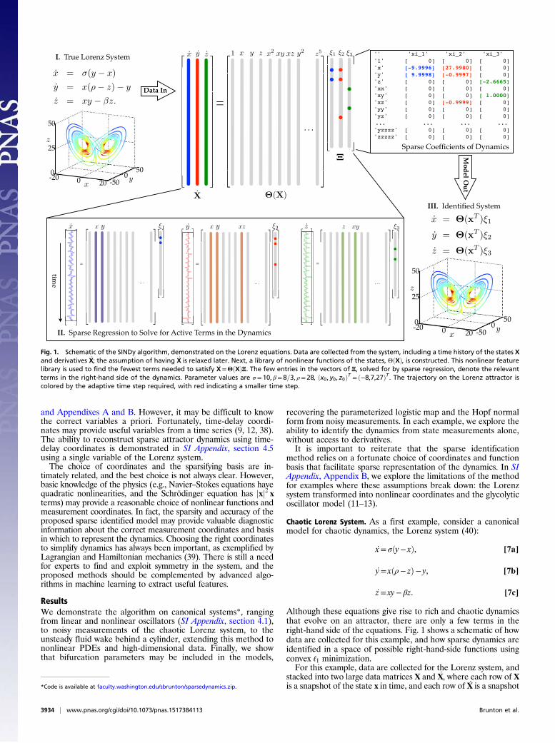
This is illustrated in Fig. 1. Each column ξk of Ξ is a sparse vectorof coefficients determining which terms are active in the right-hand side for one of the row equations _xk = fkðxÞ in Eq. 1. Once Ξhas been determined, a model of each row of the governingequations may be constructed as follows:

_xk = fkðxÞ=Θ�xT

�ξk. [4]

Note that ΘðxTÞ is a vector of symbolic functions of elements ofx, as opposed to ΘðXÞ, which is a data matrix. Thus,

_x= fðxÞ=ΞT�Θ�xT��T . [5]

Each column of Eq. 3 requires a distinct optimization to findthe sparse vector of coefficients ξk for the kth row equation. Wemay also normalize the columns of ΘðXÞ, especially when entriesof X are small, as discussed in the SI Appendix.For examples in this paper, the matrix ΘðXÞ has size m× p,

where p is the number of candidate functions, and m � p be-cause there are more data samples than functions; this is possiblein a restricted basis, such as the polynomial basis in Eq. 2. Inpractice, it may be helpful to test many different function basesand use the sparsity and accuracy of the resulting model as adiagnostic tool to determine the correct basis to represent thedynamics in. In SI Appendix, Appendix B, two examples are ex-plored where the sparse identification algorithm fails because thedynamics are not sparse in the chosen basis.Realistically, often only X is available, and _X must be ap-

proximated numerically, as in all of the continuous-time exam-ples below. Thus, X and _X are contaminated with noise so Eq. 3does not hold exactly. Instead,

_X=ΘðXÞΞ+ ηZ, [6]

where Z is modeled as a matrix of independent identically dis-tributed Gaussian entries with zero mean, and noise magnitudeη. Thus, we seek a sparse solution to an overdetermined systemwith noise. The least absolute shrinkage and selection operator(LASSO) (14, 15) is an ℓ1-regularized regression that promotessparsity and works well with this type of data. However, it may becomputationally expensive for very large data sets. An alternativebased on sequential thresholded least-squares is presented inCode 1 in the SI Appendix.Depending on the noise, it may be necessary to filter X and _X

before solving for Ξ. In many of the examples below, only the dataX are available, and _X are obtained by differentiation. To coun-teract differentiation error, we use the total variation regularization(32) to denoise the derivative (33). This works quite well when onlystate data X are available, as illustrated on the Lorenz system (SIAppendix, Fig. S7). Alternatively, the data X and _Xmay be filtered,for example using the optimal hard threshold for singular valuesdescribed in ref. 34. Insensitivity to noise is a critical feature of analgorithm that identifies dynamics from data (11–13).Often, the physical system of interest may be naturally repre-

sented by a partial differential equation (PDE) in a few spatialvariables. If data are collected from a numerical discretization orfrom experimental measurements on a spatial grid, then the statedimension n may be prohibitively large. For example, in fluid dy-namics, even simple 2D and 3D flows may require tens of thou-sands up to billions of variables to represent the discretized system.The proposed method is ill-suited for a large state dimensionn, because of the factorial growth of Θ in n and because each of then row equations in Eq. 4 requires a separate optimization. Fortu-nately, many high-dimensional systems of interest evolve on a low-dimensional manifold or attractor that is well-approximated using alow-rank basis Ψ (35, 36). For example, if data X are collected for ahigh-dimensional system as in Eq. 2, it is possible to obtain a low-rank approximation using dimensionality reduction techniques,such as the proper orthogonal decomposition (POD) (35, 37).The proposed sparse identification of nonlinear dynamics

(SINDy) method depends on the choice of measurement vari-ables, data quality, and the sparsifying function basis. There is nosingle method that will solve all problems in nonlinear systemidentification, but this method highlights the importance of theseunderlying choices and can help guide the analysis. The chal-lenges of choosing measurement variables and a sparsifyingfunction basis are explored in SI Appendix, section 4.5 and Ap-pendixes A and B.Simply put, we need the right coordinates and function basis to

yield sparse dynamics; the feasibility and flexibility of these re-quirements is discussed in Discussion and SI Appendix section 4.5

Brunton et al. PNAS | April 12, 2016 | vol. 113 | no. 15 | 3933

APP

LIED

MATH

EMATICS

and Appendixes A and B. However, it may be difficult to knowthe correct variables a priori. Fortunately, time-delay coordi-nates may provide useful variables from a time series (9, 12, 38).The ability to reconstruct sparse attractor dynamics using time-delay coordinates is demonstrated in SI Appendix, section 4.5using a single variable of the Lorenz system.The choice of coordinates and the sparsifying basis are in-

timately related, and the best choice is not always clear. However,basic knowledge of the physics (e.g., Navier–Stokes equations havequadratic nonlinearities, and the Schrödinger equation has jxj2 xterms) may provide a reasonable choice of nonlinear functions andmeasurement coordinates. In fact, the sparsity and accuracy of theproposed sparse identified model may provide valuable diagnosticinformation about the correct measurement coordinates and basisin which to represent the dynamics. Choosing the right coordinatesto simplify dynamics has always been important, as exemplified byLagrangian and Hamiltonian mechanics (39). There is still a needfor experts to find and exploit symmetry in the system, and theproposed methods should be complemented by advanced algo-rithms in machine learning to extract useful features.

ResultsWe demonstrate the algorithm on canonical systems*, rangingfrom linear and nonlinear oscillators (SI Appendix, section 4.1),to noisy measurements of the chaotic Lorenz system, to theunsteady fluid wake behind a cylinder, extending this method tononlinear PDEs and high-dimensional data. Finally, we showthat bifurcation parameters may be included in the models,

recovering the parameterized logistic map and the Hopf normalform from noisy measurements. In each example, we explore theability to identify the dynamics from state measurements alone,without access to derivatives.It is important to reiterate that the sparse identification

method relies on a fortunate choice of coordinates and functionbasis that facilitate sparse representation of the dynamics. In SIAppendix, Appendix B, we explore the limitations of the methodfor examples where these assumptions break down: the Lorenzsystem transformed into nonlinear coordinates and the glycolyticoscillator model (11–13).

Chaotic Lorenz System. As a first example, consider a canonicalmodel for chaotic dynamics, the Lorenz system (40):

_x= σðy− xÞ, [7a]

_y= xðρ− zÞ− y, [7b]

_z= xy− βz. [7c]

Although these equations give rise to rich and chaotic dynamicsthat evolve on an attractor, there are only a few terms in theright-hand side of the equations. Fig. 1 shows a schematic of howdata are collected for this example, and how sparse dynamics areidentified in a space of possible right-hand-side functions usingconvex ℓ1 minimization.For this example, data are collected for the Lorenz system, and

stacked into two large data matrices X and _X, where each row of Xis a snapshot of the state x in time, and each row of _X is a snapshot

Fig. 1. Schematic of the SINDy algorithm, demonstrated on the Lorenz equations. Data are collected from the system, including a time history of the states Xand derivatives _X; the assumption of having _X is relaxed later. Next, a library of nonlinear functions of the states, ΘðXÞ, is constructed. This nonlinear featurelibrary is used to find the fewest terms needed to satisfy _X=ΘðXÞΞ. The few entries in the vectors of Ξ, solved for by sparse regression, denote the relevantterms in the right-hand side of the dynamics. Parameter values are σ = 10, β= 8=3, ρ= 28, ðx0, y0, z0ÞT = ð−8,7,27ÞT . The trajectory on the Lorenz attractor iscolored by the adaptive time step required, with red indicating a smaller time step.

*Code is available at faculty.washington.edu/sbrunton/sparsedynamics.zip.

3934 | www.pnas.org/cgi/doi/10.1073/pnas.1517384113 Brunton et al.

of the time derivative of the state _x in time. Here, the right-hand-side dynamics are identified in the space of polynomials ΘðXÞ inðx, y, zÞ up to fifth order, although other functions such assin, cos, exp, or higher-order polynomials may be included:

ΘðXÞ="xðtÞj

jyðtÞj

jzðtÞj

jxðtÞ2

j

jxðtÞyðtÞ

j

j⋯ z ðtÞ5

j

j

#.

Each column of ΘðXÞ represents a candidate function for the right-hand sideofEq.1. Becauseonly a fewof these terms are active in eachrow of f, we solve the sparse regression problem inEq. 3 to determinethe sparse vectors of coefficients Ξ= ½ ξ1 ξ2 ⋯ ξn � that determinewhich terms are active in the dynamics. This is illustrated schemati-cally in Fig. 1, where sparse vectors ξk are found to represent thederivative _xk as a linear combination of the fewest terms in ΘðXÞ.In the Lorenz example, the ability to capture dynamics on the

attractor is more important than the ability to predict an individualtrajectory, because chaos will quickly cause any small variations ininitial conditions or model coefficients to diverge exponentially.As shown in Fig. 1, the sparse model accurately reproduces theattractor dynamics from chaotic trajectory measurements. Thealgorithm not only identifies the correct terms in the dynamics, butit accurately determines the coefficients to within .03% of the truevalues. We also explore the identification of the dynamics whenonly noisy state measurements are available (SI Appendix, Fig. S7).The correct dynamics are identified, and the attractor is preservedfor surprisingly large noise values. In SI Appendix, section 4.5, wereconstruct the attractor dynamics in the Lorenz system usingtime-delay coordinates from a single measurement xðtÞ.PDE for Vortex Shedding Behind an Obstacle.The Lorenz system is alow-dimensional model of more realistic high-dimensional PDEmodels for fluid convection in the atmosphere. Many systems ofinterest are governed by PDEs (24), such as weather and climate,epidemiology, and the power grid, to name a few. Each of theseexamples is characterized by big data, consisting of large spatiallyresolved measurements consisting of millions or billions of statesand spanning orders of magnitude of scale in both space andtime. However, many high-dimensional, real-world systems evolveon a low-dimensional attractor, making the effective dimensionmuch smaller (35).Here we generalize the SINDy method to an example in fluid dy-

namics that typifies many of the challenges outlined above. In thecontext of data from a PDE, our algorithm shares some connections tothe dynamic mode decomposition, which is a linear dynamic regression

(41–43). Data are collected for the fluid flow past a cylinder atReynolds number 100 using direct numerical simulations of the 2DNavier–Stokes equations (44, 45). The nonlinear dynamic relationshipbetween the dominant coherent structures is identified from these flow-field measurements with no knowledge of the governing equations.The flow past a cylinder is a particularly interesting example be-

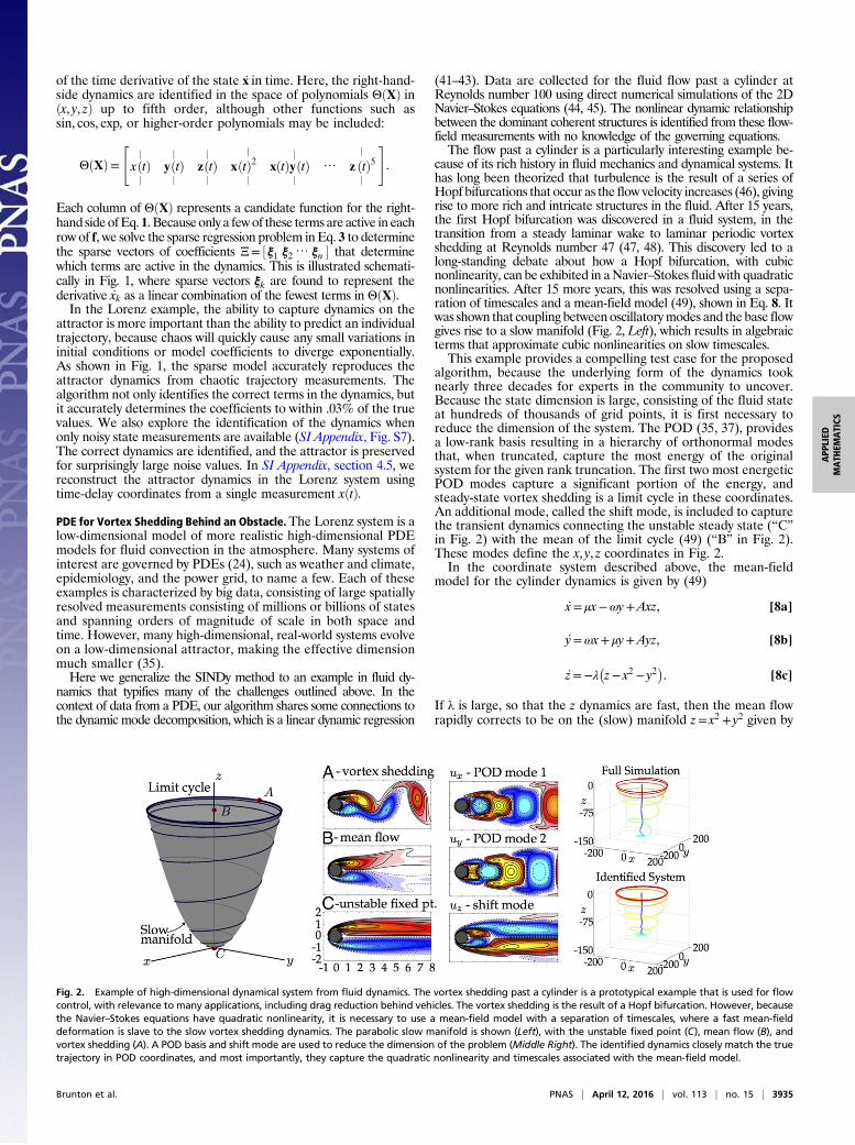
cause of its rich history in fluid mechanics and dynamical systems. Ithas long been theorized that turbulence is the result of a series ofHopf bifurcations that occur as the flow velocity increases (46), givingrise to more rich and intricate structures in the fluid. After 15 years,the first Hopf bifurcation was discovered in a fluid system, in thetransition from a steady laminar wake to laminar periodic vortexshedding at Reynolds number 47 (47, 48). This discovery led to along-standing debate about how a Hopf bifurcation, with cubicnonlinearity, can be exhibited in aNavier–Stokes fluid with quadraticnonlinearities. After 15 more years, this was resolved using a sepa-ration of timescales and a mean-field model (49), shown in Eq. 8. Itwas shown that coupling between oscillatorymodes and the base flowgives rise to a slow manifold (Fig. 2, Left), which results in algebraicterms that approximate cubic nonlinearities on slow timescales.This example provides a compelling test case for the proposed

algorithm, because the underlying form of the dynamics tooknearly three decades for experts in the community to uncover.Because the state dimension is large, consisting of the fluid stateat hundreds of thousands of grid points, it is first necessary toreduce the dimension of the system. The POD (35, 37), providesa low-rank basis resulting in a hierarchy of orthonormal modesthat, when truncated, capture the most energy of the originalsystem for the given rank truncation. The first two most energeticPOD modes capture a significant portion of the energy, andsteady-state vortex shedding is a limit cycle in these coordinates.An additional mode, called the shift mode, is included to capturethe transient dynamics connecting the unstable steady state (“C”in Fig. 2) with the mean of the limit cycle (49) (“B” in Fig. 2).These modes define the x, y, z coordinates in Fig. 2.In the coordinate system described above, the mean-field

model for the cylinder dynamics is given by (49)

_x= μx−ωy+Axz, [8a]

_y=ωx+ μy+Ayz, [8b]

_z=−λ�z− x2 − y2

�. [8c]

If λ is large, so that the z dynamics are fast, then the mean flowrapidly corrects to be on the (slow) manifold z= x2 + y2 given by

Fig. 2. Example of high-dimensional dynamical system from fluid dynamics. The vortex shedding past a cylinder is a prototypical example that is used for flowcontrol, with relevance to many applications, including drag reduction behind vehicles. The vortex shedding is the result of a Hopf bifurcation. However, becausethe Navier–Stokes equations have quadratic nonlinearity, it is necessary to use a mean-field model with a separation of timescales, where a fast mean-fielddeformation is slave to the slow vortex shedding dynamics. The parabolic slow manifold is shown (Left), with the unstable fixed point (C), mean flow (B), andvortex shedding (A). A POD basis and shift mode are used to reduce the dimension of the problem (Middle Right). The identified dynamics closely match the truetrajectory in POD coordinates, and most importantly, they capture the quadratic nonlinearity and timescales associated with the mean-field model.

Brunton et al. PNAS | April 12, 2016 | vol. 113 | no. 15 | 3935

APP

LIED

MATH

EMATICS

the amplitude of vortex shedding. When substituting this alge-braic relationship into Eqs. 8a and 8b, we recover the Hopfnormal form on the slow manifold.With a time history of these three coordinates, the proposed al-

gorithm correctly identifies quadratic nonlinearities and reproducesa parabolic slow manifold. Note that derivative measurements arenot available, but are computed from the state variables. In-terestingly, when the training data do not include trajectories thatoriginate off of the slow manifold, the algorithm incorrectly iden-tifies cubic nonlinearities, and fails to identify the slow manifold.

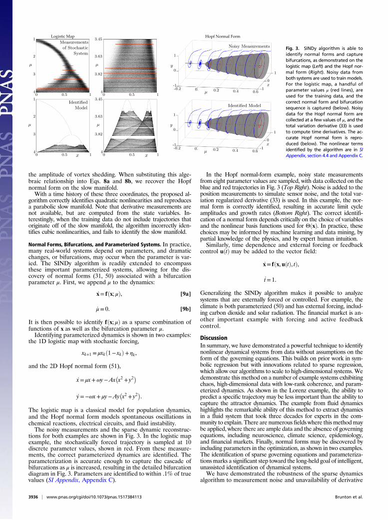
Normal Forms, Bifurcations, and Parameterized Systems. In practice,many real-world systems depend on parameters, and dramaticchanges, or bifurcations, may occur when the parameter is var-ied. The SINDy algorithm is readily extended to encompassthese important parameterized systems, allowing for the dis-covery of normal forms (31, 50) associated with a bifurcationparameter μ. First, we append μ to the dynamics:

_x= fðx; μÞ, [9a]

_μ= 0. [9b]

It is then possible to identify fðx; μÞ as a sparse combination offunctions of x as well as the bifurcation parameter μ.Identifying parameterized dynamics is shown in two examples:

the 1D logistic map with stochastic forcing,

xk+1 = μxkð1− xkÞ+ ηk,

and the 2D Hopf normal form (51),

_x= μx+ωy−Ax�x2 + y2

�_y=−ωx+ μy−Ay

�x2 + y2

�.

The logistic map is a classical model for population dynamics,and the Hopf normal form models spontaneous oscillations inchemical reactions, electrical circuits, and fluid instability.The noisy measurements and the sparse dynamic reconstruc-

tions for both examples are shown in Fig. 3. In the logistic mapexample, the stochastically forced trajectory is sampled at 10discrete parameter values, shown in red. From these measure-ments, the correct parameterized dynamics are identified. Theparameterization is accurate enough to capture the cascade ofbifurcations as μ is increased, resulting in the detailed bifurcationdiagram in Fig. 3. Parameters are identified to within .1% of truevalues (SI Appendix, Appendix C).

In the Hopf normal-form example, noisy state measurementsfrom eight parameter values are sampled, with data collected on theblue and red trajectories in Fig. 3 (Top Right). Noise is added to theposition measurements to simulate sensor noise, and the total var-iation regularized derivative (33) is used. In this example, the nor-mal form is correctly identified, resulting in accurate limit cycleamplitudes and growth rates (Bottom Right). The correct identifi-cation of a normal form depends critically on the choice of variablesand the nonlinear basis functions used for ΘðxÞ. In practice, thesechoices may be informed by machine learning and data mining, bypartial knowledge of the physics, and by expert human intuition.Similarly, time dependence and external forcing or feedback

control uðtÞ may be added to the vector field:

_x= fðx, uðtÞ, tÞ,

_t= 1.

Generalizing the SINDy algorithm makes it possible to analyzesystems that are externally forced or controlled. For example, theclimate is both parameterized (50) and has external forcing, includ-ing carbon dioxide and solar radiation. The financial market is an-other important example with forcing and active feedbackcontrol.

DiscussionIn summary, we have demonstrated a powerful technique to identifynonlinear dynamical systems from data without assumptions on theform of the governing equations. This builds on prior work in sym-bolic regression but with innovations related to sparse regression,which allow our algorithms to scale to high-dimensional systems.Wedemonstrate this method on a number of example systems exhibitingchaos, high-dimensional data with low-rank coherence, and param-eterized dynamics. As shown in the Lorenz example, the ability topredict a specific trajectory may be less important than the ability tocapture the attractor dynamics. The example from fluid dynamicshighlights the remarkable ability of this method to extract dynamicsin a fluid system that took three decades for experts in the com-munity to explain. There are numerous fields where this methodmaybe applied, where there are ample data and the absence of governingequations, including neuroscience, climate science, epidemiology,and financial markets. Finally, normal forms may be discovered byincluding parameters in the optimization, as shown in two examples.The identification of sparse governing equations and parameteriza-tions marks a significant step toward the long-held goal of intelligent,unassisted identification of dynamical systems.We have demonstrated the robustness of the sparse dynamics

algorithm to measurement noise and unavailability of derivative

Fig. 3. SINDy algorithm is able toidentify normal forms and capturebifurcations, as demonstrated on thelogistic map (Left) and the Hopf nor-mal form (Right). Noisy data fromboth systems are used to train models.For the logistic map, a handful ofparameter values μ (red lines), areused for the training data, and thecorrect normal form and bifurcationsequence is captured (below). Noisydata for the Hopf normal form arecollected at a few values of μ, and thetotal variation derivative (33) is usedto compute time derivatives. The ac-curate Hopf normal form is repro-duced (below). The nonlinear termsidentified by the algorithm are in SIAppendix, section 4.4 and Appendix C.

3936 | www.pnas.org/cgi/doi/10.1073/pnas.1517384113 Brunton et al.

measurements in the Lorenz system (SI Appendix, Figs. S6 andS7), logistic map (SI Appendix, section 4.4.1), and Hopf normalform (SI Appendix, section 4.4.2) examples. In each case, thesparse regression framework appears well-suited to measurementand process noise, especially when derivatives are smoothed usingthe total-variation regularized derivative.A significant outstanding issue in the above approach is the correct

choice of measurement coordinates and the choice of sparsifyingfunction basis for the dynamics. As shown in SI Appendix, AppendixB, the algorithm fails to identify an accurate sparse model when themeasurement coordinates and function basis are not amenable tosparse representation. In the successful examples, the coordinatesand function spaces were somehow fortunate in that they enabledsparse representation. There is no simple solution to this challenge,and there must be a coordinated effort to incorporate expertknowledge, feature extraction, and other advanced methods. How-ever, in practice, there may be some hope of obtaining the correctcoordinate system and function basis without knowing the solutionahead of time, because we often know something about the physicsthat guide the choice of function space. The failure to identify anaccurate sparse model also provides valuable diagnostic informationabout the coordinates and basis. If we have fewmeasurements, thesemay be augmented using time-delay coordinates, as demonstratedon the Lorenz system (SI Appendix, section 4.5). When there are toomany measurements, we may extract coherent structures using

dimensionality reduction. We also demonstrate the use of poly-nomial bases to approximate Taylor series of nonlinear dynamics (SIAppendix, Appendix A). The connection between sparse optimiza-tion and dynamical systems will hopefully spur developments toautomate and improve these choices.Data science is not a panacea for all problems in science and en-

gineering, but used in the right way, it provides a principled approachto maximally leverage the data that we have and inform what newdata to collect. Big data are happening all across the sciences, wherethe data are inherently dynamic, and where traditional approachesare prone to overfitting. Data discovery algorithms that produceparsimonious models are both rare and desirable. Data science willonly becomemore critical to efforts in science in engineering, such asunderstanding the neural basis of cognition, extracting and predictingcoherent changes in the climate, stabilizing financial markets, man-aging the spread of disease, and controlling turbulence, where dataare abundant, but physical laws remain elusive.

ACKNOWLEDGMENTS. We are grateful for discussions with Bing Bruntonand Bernd Noack, and for insightful comments from the referees. We alsothank Tony Roberts and Jean-Christophe Loiseau. S.L.B. acknowledgessupport from the University of Washington. J.L.P. thanks Bill and MelindaGates for their support of the Institute for Disease Modeling and theirsponsorship through the Global Good Fund. J.N.K. acknowledges supportfrom the US Air Force Office of Scientific Research (FA9550-09-0174).

1. Jordan MI, Mitchell TM (2015) Machine learning: Trends, perspectives, and prospects.

Science 349(6245):255–260.2. Marx V (2013) Biology: The big challenges of big data. Nature 498(7453):255–260.3. Bongard J, Lipson H (2007) Automated reverse engineering of nonlinear dynamical

systems. Proc Natl Acad Sci USA 104(24):9943–9948.4. Schmidt M, Lipson H (2009) Distilling free-form natural laws from experimental data.

Science 324(5923):81–85.5. Koza JR (1992) Genetic Programming: On the Programming of Computers by Means

of Natural Selection (MIT Press, Cambridge, MA), Vol 1.6. Crutchfield JP, McNamara BS (1987) Equations of motion from a data series. Complex

Syst 1(3):417–452.7. Kevrekidis IG, et al. (2003) Equation-free, coarse-grained multiscale computation: Enabling

microscopic simulators to perform system-level analysis. Commun Math Sci 1(4):715–762.8. Sugihara G, et al. (2012) Detecting causality in complex ecosystems. Science 338(6106):

496–500.9. Ye H, et al. (2015) Equation-free mechanistic ecosystem forecasting using empirical

dynamic modeling. Proc Natl Acad Sci USA 112(13):E1569–E1576.10. Roberts AJ (2014) Model Emergent Dynamics in Complex Systems (SIAM, Philadelphia).11. Schmidt MD, et al. (2011) Automated refinement and inference of analytical models

for metabolic networks. Phys Biol 8(5):055011.12. Daniels BC, Nemenman I (2015) Automated adaptive inference of phenomenological

dynamical models. Nat Commun 6:8133.13. Daniels BC, Nemenman I (2015) Efficient inference of parsimonious phenomenolog-

ical models of cellular dynamics using S-systems and alternating regression. PLoS One

10(3):e0119821.14. Tibshirani R (1996) Regression shrinkage and selection via the lasso. J R Stat Soc, B

58(1):267–288.15. Hastie T, Tibshirani R, Friedman J (2009) The Elements of Statistical Learning

(Springer, New York), Vol 2.16. James G, Witten D, Hastie T, Tibshirani R (2013) An Introduction to Statistical Learning

(Springer, New York).17. Donoho DL (2006) Compressed sensing. IEEE Trans Inf Theory 52(4):1289–1306.18. Candès EJ, Romberg J, Tao T (2006) Robust uncertainty principles: Exact signal reconstruction

from highly incomplete frequency information. IEEE Trans Inf Theory 52(2):489–509.19. Candès EJ, Romberg J, Tao T (2006) Stable signal recovery from incomplete and in-

accurate measurements. Commun Pure Appl Math 59(8):1207–1223.20. Candès EJ, Wakin MB (2008) An introduction to compressive sampling. IEEE Signal

Processing Magazine 25(2):21–30.21. Baraniuk RG (2007) Compressive sensing. IEEE Signal Process Mag 24(4):118–120.22. Tropp JA, Gilbert AC (2007) Signal recovery from random measurements via or-

thogonal matching pursuit. IEEE Trans Inf Theory 53(12):4655–4666.23. Wang WX, Yang R, Lai YC, Kovanis V, Grebogi C (2011) Predicting catastrophes in

nonlinear dynamical systems by compressive sensing. Phys Rev Lett 106(15):154101.24. Schaeffer H, Caflisch R, Hauck CD, Osher S (2013) Sparse dynamics for partial differ-

ential equations. Proc Natl Acad Sci USA 110(17):6634–6639.25. Ozolinš V, Lai R, Caflisch R, Osher S (2013) Compressed modes for variational problems

in mathematics and physics. Proc Natl Acad Sci USA 110(46):18368–18373.26. Mackey A, Schaeffer H, Osher S (2014) On the compressive spectral method.

Multiscale Model Simul 12(4):1800–1827.

27. Brunton SL, Tu JH, Bright I, Kutz JN (2014) Compressive sensing and low-rank librariesfor classification of bifurcation regimes in nonlinear dynamical systems. SIAM J ApplDyn Syst 13(4):1716–1732.

28. Proctor JL, Brunton SL, Brunton BW, Kutz JN (2014) Exploiting sparsity and equation-freearchitectures in complex systems (invited review). Eur Phys J Spec Top 223:2665–2684.

29. Bai Z, et al. (2014) Low-dimensional approach for reconstruction of airfoil data viacompressive sensing. AIAA J 53(4):920–930.

30. Arnaldo I, O’Reilly UM, Veeramachaneni K (2015) Building predictive models viafeature synthesis. Proceedings of the 2015 Annual Conference on Genetic andEvolutionary Computation (ACM, New York), pp 983–990.

31. Holmes P, Guckenheimer J (1983) Nonlinear oscillations, dynamical systems, and bi-furcations of vector fields. Applied Mathematical Sciences (Springer, Berlin), Vol 42.

32. Rudin LI, Osher S, Fatemi E (1992) Nonlinear total variation based noise removal al-gorithms. Physica D 60(1):259–268.

33. Chartrand R (2011) Numerical differentiation of noisy, nonsmooth data. ISRN AppliedMathematics 2011(2011):164564.

34. Gavish M, Donoho DL (2014) The optimal hard threshold for singular values is 4/ffiffiffi3

p.

IEEE Trans Inf Theory 60(8):5040–5053.35. Holmes PJ, Lumley JL, Berkooz G, Rowley CW (2012) Turbulence, Coherent Structures,

Dynamical Systems and Symmetry, Cambridge Monographs in Mechanics (CambridgeUniv Press, Cambridge, UK), 2nd Ed.

36. Majda AJ, Harlim J (2007) Information flow between subspaces of complex dynamicalsystems. Proc Natl Acad Sci USA 104(23):9558–9563.

37. Berkooz G, Holmes P, Lumley JL (1993) The proper orthogonal decomposition in theanalysis of turbulent flows. Annu Rev Fluid Mech 23:539–575.

38. Takens F (1981) Detecting strange attractors in turbulence. Lect Notes Math 898:366–381.39. Marsden JE, Ratiu TS (1999) Introduction to Mechanics and Symmetry (Springer,

New York), 2nd Ed.40. Lorenz EN (1963) Deterministic nonperiodic flow. J Atmos Sci 20:130–141.41. Rowley CW, Mezi�c I, Bagheri S, Schlatter P, Henningson D (2009) Spectral analysis of

nonlinear flows. J Fluid Mech 645:115–127.42. Schmid PJ (2010) Dynamic mode decomposition of numerical and experimental data.

J Fluid Mech 656:5–28.43. Mezic I (2013) Analysis of fluid flows via spectral properties of the Koopman operator.

Annu Rev Fluid Mech 45:357–378.44. Taira K, Colonius T (2007) The immersed boundary method: A projection approach.

J Comput Phys 225(2):2118–2137.45. Colonius T, Taira K (2008) A fast immersed boundary method using a nullspace ap-

proach and multi-domain far-field boundary conditions. Comput Methods Appl MechEng 197:2131–2146.

46. Ruelle D, Takens F (1971) On the nature of turbulence. CommunMath Phys 20:167–192.47. Jackson CP (1987) A finite-element study of the onset of vortex shedding in flow past

variously shaped bodies. J Fluid Mech 182:23–45.48. Zebib Z (1987) Stability of viscous flow past a circular cylinder. J Eng Math 21:155–165.49. Noack BR, Afanasiev K, Morzynski M, Tadmor G, Thiele F (2003) A hierarchy of low-

dimensional models for the transient and post-transient cylinder wake. J Fluid Mech497:335–363.

50. Majda AJ, Franzke C, Crommelin D (2009) Normal forms for reduced stochastic climatemodels. Proc Natl Acad Sci USA 106(10):3649–3653.

51. Marsden JE, McCracken M (1976) The Hopf Bifurcation and Its Applications (Springer,New York), Vol 19.

Brunton et al. PNAS | April 12, 2016 | vol. 113 | no. 15 | 3937

APP

LIED

MATH

EMATICS