Discussion Papers No. 479, October 2006 Statistics Norway, Research Department

Torgeir Ericson

Direct load control of residential water heaters

Abstract: In Norway there is a growing concern that electricity production and transmission may not meet the demand in peak-load situations. It is therefore important to evaluate the potential of different demand side measures that may contribute to reduce peak load. This paper analyses data from an experiment where residential water heaters were automatically disconnected during peak periods of the day. A model of hourly electricity consumption is used to evaluate the effects on the load of the disconnections. The results indicate an average consumption reduction per household of approximately 0.5 kWh/h during disconnection, and an additional average increase in consumption the following hour, due to the payback effect, of approximately 0.2 kWh/h.

Keywords: Direct load control; Demand response; Load management; Water heaters

JEL classification: D10, Q41

Acknowledgement: I am very grateful to Kjetil Telle and Bente Halvorsen for advice and helpful discussions. I also appreciate comments on earlier drafts of this paper from Terje Skjerpen, Petter Vegard Hansen, Knut Reidar Wangen, Annegrete Bruvoll, Trond Gärtner, Hanne Sæle and Per Finden, and programming assistance from Hilde Madsen.

Address: Torgeir Ericson, Statistics Norway, Research Department. E-mail: toe@ssb.no

Discussion Papers comprise research papers intended for international journals or books. A preprint of a Discussion Paper may be longer and more elaborate than a standard journal article, as it may include intermediate calculations and background material etc.

Abstracts with downloadable Discussion Papers in PDF are available on the Internet: http://www.ssb.no http://ideas.repec.org/s/ssb/dispap.html For printed Discussion Papers contact: Statistics Norway Sales- and subscription service NO-2225 Kongsvinger Telephone: +47 62 88 55 00 Telefax: +47 62 88 55 95 E-mail: Salg-abonnement@ssb.no

3

1. Introduction

Peak electricity consumption in Norway has been increasing, and is expected to continue to

increase in the years to come (Glende et al., 2005). However, since deregulation of the electricity

market in 1991, new investment in power generation has been at a low level (Bye and Hope,

2005). Periods with extreme cold weather have revealed a vulnerable production and distribution

system, as consumption in such peak situations has been close to capacity. This calls for a flexible

demand side with the potential of reducing loads in peak situations to relieve the constrained

system. Demand response may consequently defer the need for costly augmentation of the

electricity grid or power production.

Direct load control and time-differentiated tariffs are two measures to obtain demand

response that have been tested and used worldwide. A direct load control programme often

involves customers who are willing to offer electricity-consuming appliances for load reduction if

they are compensated economically. Traditional interruptible programmes have paid their

customers in advance for participating, for example, through rate discounts. An example is an air

conditioner and water heater load programme in the USA, where customers are provided with

discounts on their electricity bill if they participate in the programme (Xcel Energy, 2005). The

customers receive $US6 for each month in the summer if they allow 15–20 minutes cycling of

their air conditioner in the hot summer months and an additional $US2 each month for the whole

year if they allow their water heaters to be disconnected for six-hour periods on hot summer days

or cold winter days. The utility is only allowed to control the appliances for a maximum of 300

hours per year. In 2001, when approximately 280,000 residential customers were on the

programme, electricity consumption was reduced by 330 MW in peak situations. Another example

where water heaters are under direct control is an Australian programme involving 355,000 water

heaters. This control reduces peak electricity consumption by 389 MW. The incentive for the

customers to participate in the programme is lower rates for their water heating (Charles River

Associates, 2003). A direct load control programme in the USA controls air conditioning, central

4

electric heaters, electric water heaters and swimming pool pumps. A total of 800,000 controlled

points provides 1,000 MW of demand reduction in normal operation, and 2,000 MW in emergency

situations (Malemezian, 2004).

Direct load control is often combined with time-differentiated pricing, such as time-of-use

or dynamic pricing, to assist reduction of consumption during high-priced peak periods. King

(2004) found load reductions for programmes that integrated dynamic pricing with automated load

control to be on average 53% larger than load reductions in programmes with load control alone.

He further found the integrated programmes give 102% larger reductions than programmes with

only dynamic pricing, i.e., over twice the reduction.

Water heaters constitute approximately 10% of the electricity consumption in Norwegian

households (Larsen and Nesbakken, 2005). Direct load control of water heaters may therefore have

a large demand response potential which is important to quantify. This paper provides such

estimates by studying data from a large-scale Norwegian project where load control of residential

water heaters was applied. Hourly measurement of the electricity consumption from 475

households, number of hours of daylight each day, and the local temperature and wind speed in a

six-month period from November 2003 to May 2004, provide a large panel data set that we

analyse with statistical methods. We develop a fixed effects regression model of hourly electricity

consumption and use it to evaluate the impact of the water heater control on households’ load

curves.

The results from the analysis show significant electricity consumption reductions during

disconnections of the water heaters. The results also indicate additional consumption when the

heaters are reconnected due to the so-called “payback” or “cold load pickup” effect (which is

explained in the next section) which may cause a new peak in the electricity system, suggesting

cycling the control events may be necessary.

Section 2 describes factors that may influence the load reducing potential and the payback

effect experienced when applying direct load control of water heaters, Section 3 describes the

experiment and the data that are analysed and Section 4 describes the method and the models that

are used. The results are evaluated in Section 5 and the last section concludes.

5

2. Water heaters and load control

When water heaters are used for direct load control, essentially all of the energy not supplied

to the heaters when they are disconnected from the electricity supply will be required when they

are reconnected. When switched on, all affected heaters that were supposed to be on during the

control period, will start recovering from the interruption at the same time. Unless handled

properly, this payback effect may have the undesired effect of creating a new peak in the

electricity system. It is thus useful to discuss some causes for the effects experienced when water

heaters are used for load control. This section describes some of these factors.

A water heater is used to heat and store hot water. A typical Norwegian residential water

heater holds 200 litres and has a rated heating element capacity of 2 kW. The heat loss from a tank

is approximately 0.1 kWh/h at a temperature of 75°C (HiO, 2005). It takes approximately 2.3

hours for a full heated tank to drop in temperature by 1°C in stand-by mode, i.e., when no hot

water is drawn from the tank. The water heater’s thermostat is usually a bimetallic strip with a

dead-band of approximately 4°C. This means that the heating element will start operating when

temperature falls below 73°C and stop operating when the temperature exceeds 77°C. Due to the

thermostat’s dead-band, a full heated tank in stand-by mode will require approximately nine hours

before the thermostat activates the heating element as a result of heat loss. Orphelin and Adnot

(1999) found that most heaters are operating due to the households’ usage of water rather than due

to heat losses.

When a household uses hot water, the water is drawn from the top of the tank. At the same

time, cold water refills at the bottom of the tank. The thermostat is placed a few centimetres above

the bottom, and will respond to a temperature drop by activating the heating element. A hand wash

may use only a few litres of hot water. The energy use is accordingly low, and a heater will need to

operate for only a few minutes to restore the energy used.1 A large family may use 14 kWh when

all members are showering, which requires the heating element to operate for seven hours

1 However, small amounts of water use may not activate the heating element. This is explained below.

6

afterwards. Those two examples may represent a range of energy use due to hot water use during

morning hours in different households.

Because hot water can be stored for long periods of time without significant heat loss in a

well-insulated tank, it is well suited to heat water at one period of the day and use this water at

another period. Direct load control of water heaters has therefore been widely applied to reduce

peak load. The idea is to turn off the electricity supply to a large number of heaters during peak

periods. If all heaters have elements of 2 kW-rated capacity, the maximum theoretical load

reduction achievable is 2 kWh/h per heater. However, the average reduction of load per household

is likely to be less, due to diversity with respect to the timing of the hot water usage between

households.

Two principle outlines of energy recover in water heaters, with and without disconnections

of the heaters, in hypothetical household groups with different usage (high and low) of hot water

are shown in parts (a) and (b) of Fig. 1. The heating element capacity is assumed to be the same

for all households. For illustrative purposes it is assumed that the starting point for hot water usage

is distributed uniformly over the hours around the control event.

1 2 . . . . . . . . . . . . n

Disconnection Reconnection

time t0 t1 t3

Disconnection Reconnection

time t1 t0 t2

1 2 . . . . . . . . . . . . n

Consumption of water (and operation of heating element)

Operation of heating element

Payback period

(a) (b)

Fig. 1.

Energy recovering of water heaters with and without disconnections for households with a high level

of hot water consumption, 1,…,n (a), and low level of hot water consumption, 1,…,n (b)

7

Fig. 1 shows water heaters of two household groups with n households in each group. There

is one heater at each “line”. The shaded and the white areas indicate the operating period for the

heaters under normal conditions if a disconnection is not made. The shaded area indicates the

period of hot water use (it is assumed that the heaters start operating immediately after hot water is

drawn, i.e., at the beginning of the shaded area). The households use hot water at different times;

in each group, number 1 starts consuming hot water first and number n last. A disconnection starts

at t0 and finishes at t1, when the heaters are reconnected. The black area indicates the period when

the heaters recover energy in the situation where a disconnection has occurred. The black area is

simply the part of the energy recovery period that could not be accomplished due to the

disconnection and which is postponed compared to the normal situation, without the

disconnection. Approximately the same amount of energy that would normally be consumed

during a disconnection will be consumed after the heater is reconnected.2 This demand will be

added to the system load and give rise to consumption that would normally not exist if load control

did not occur. This payback effect is therefore the result of a disturbance in the natural diversity of

the heaters used for load control (see for example Rau and Graham (1979) and van Tonder and

Lane (1996) for a similar discussion).

Fig. 1(a) shows households with a high level of hot water usage. It can be seen that the

disconnection affects the first water heater only slightly. The heater has nearly finished recovering

the energy loss when it is disconnected; the final part of its restoration of the energy must wait

until the heater is reconnected. Disconnection of this water heater will contribute little to load

reduction in the electricity system. Nevertheless, the heater will contribute with its full-rated

capacity at the time of reconnection, although only for a short time. To some extent, this will also

be the case for the second and third heaters. The heaters in the middle of the figure will, however,

contribute to a reduction with their rated capacity during the entire disconnection period. In

addition, as these heaters start operating close to the time of disconnection and have a long

2 There will be a very small energy saving effect as the heaters are left for a period at a lower temperature than they otherwise would have been.

8

recovery period, their payback contribution occurs after t1. At every moment during the

disconnection period, it can be seen that the disconnection affects 10 heaters. When reconnected,

only five heaters contribute to the payback effect at every moment until t3. In this example the

power demand added to the system load after a disconnection is therefore only half the size of the

reduced power demand during the disconnection. The system load curve will return to normal

shape after t3, when all heaters affected by the load control have restored the energy consumed by

the hot water use.

Fig. 1(b) shows households with a low level of hot water consumption. Their contribution to

load reduction in the electricity system is small, and the disconnection has no effect on most of the

heaters. For those that are affected, only one heater is disconnected in a certain time interval

whereas five heaters will start operating simultaneously when reconnected, giving a payback effect

from t1 to t2. The power demand added to the system load after a disconnection is five times the

size of the reduced power demand during the disconnection. Furthermore, the size of the payback

is the same as from the high hot water consumers in Fig. 1(a). The system load curve will however

quickly return to normal shape (after t2), when all heaters affected by the load control have

restored the energy consumed by the hot water usages.

Parts (a) and (b) of Fig. 2 illustrate the discussion above with load curves during a day with

and without disconnection of water heaters for the two customer groups.

1 2 3 4 5 6 7 8 9 10 11 12 13 14 15 16 17 18 19 20 21 22 23 24Hour

kW

Load without disconnectionLoad with disconnection

1 2 3 4 5 6 7 8 9 10 11 12 13 14 15 16 17 18 19 20 21 22 23 24Hour

kW

Load without disconnectionLoad with disconnection

1 2 3 4 5 6 7 8 9 10 11 12 13 14 15 16 17 18 19 20 21 22 23 24

Hour

kW

Load without disconnectionLoad with disconnection

1 2 3 4 5 6 7 8 9 10 11 12 13 14 15 16 17 18 19 20 21 22 23 24

Hour

kW

Load without disconnectionLoad with disconnection

1 2 3 4 5 6 7 8 9 10 11 12 13 14 15 16 17 18 19 20 21 22 23 24

Hour

kW

Load without disconnectionLoad with disconnection

(a) (b)

Fig. 2.

Load curves with and without disconnection for households with a high level of hot water

consumption (a), and low level of hot water consumption (b)

time t0 t1 t3 time t0 t2t1

9

These simplified examples indicate some effects experienced when heaters are used in load

control programmes. Consumption is shifted out of the disconnection period to a later period. The

payback effect will then give rise to extra consumption in the system load that would not have

taken place otherwise. The figure illustrates that the low hot water consumers contribute little to

reducing the load during the disconnection, but still create a high, although brief, peak when

reconnected. This suggests that households with the highest consumption of hot water may be the

target group in a direct load control programme.

The above discussion illustrates some effects that may occur due to differing amounts of hot

water consumption among households in a direct water heater load control programme. Further,

the capacity of the heating elements of the water heaters will influence the effects. Given two

consumer groups of equal size and with similar amounts of hot water consumption distributed

equally over time, heaters with a low-rated heating element capacity will require a longer time to

restore energy than those with high capacity, and the demand during restoration will be smaller.

Heaters with a high heating element capacity will contribute the same demand reduction during the

disconnection as those with the low-element capacity, but will yield a higher payback demand,

although over a shorter period of time, before water temperature is restored.

The inlet temperature of water to the tanks also influences the impact on the load curve from

control events. Low inlet temperature will contribute to longer heating periods and vice versa.

The frequency of hot water use may contribute to different impacts from load control,

depending on the region where it is applied. A survey of Norwegians’ showering habits revealed

that the frequency of showers differed between regions. For example, the percentages of citizens

showering daily differed from 31% in one region to 66% in another region (Pettersen, 2006).

The timing of the households’ hot water consumption may also be important. Most people in

Norway start their day from 5 to 8 am (Vaage, 2002). This suggests that a large share of the water

heaters in Norway are operating around these morning hours (around 7 to 9 am). For the evening,

the proportion of people that are home from work and have a meal is highest around 4 to 5 pm.

The proportion of households performing household work is highest around 6 pm. Disconnections

occurring around those two periods of the day (morning and afternoon) may then give the largest

10

consumption reductions since this will probably affect a high proportion of the households’

heaters.

The design of the heater may also be important. A tank will always contain a volume of

water below the heating element that remains unheated, and this unheated volume will be larger if

the heating element is installed horizontally than if it is tilted downwards inside the tank (the

thermostat is placed above the element for both designs). When hot water is drawn, the unheated

water will be pushed upwards and activate the thermostat. Therefore, because the unheated water

is just below the thermostat in the horizontal design, use of even small volumes of hot water will

activate the thermostat. In the downward-tilted design, the unheated water is further below and

larger volumes of hot water use are allowed before the cold water reaches and activates the

thermostat. Furthermore, some heaters are designed with a cold-water distributor, which decreases

the velocity of the inlet water so that the water at the bottom is blended to a lesser degree. This

allows larger volumes of hot water to be drawn without activating the heater.

The length of a disconnection will also influence the size of the initial payback demand from

all households affected by the control event, since a longer disconnection period affects more

heaters.

Therefore, load control carried out in different areas may give different load reductions and

different payback effects if, for example, hot water consumption behaviour, types of water heaters,

etc., differ between areas due to differing demographic characteristics of the households (see also

Gustavson et al. (1993), for a discussion of some of these factors).

3. Experimental data

The project “End-user Flexibility by Efficient Use of Information and Communication

Technology” (2001–2004) was a Norwegian large-scale project where automatic meter reading

and direct load control technology were installed at electricity consumers’ premises (chiefly

residential). We used data from this project to study the effect on households’ loads caused by

direct load control of their water heaters.

11

3.1. Direct load control of water heaters

The automatic meter reading and direct load control technology enabled hourly metering of

each household’s electricity consumption throughout the test period and direct control of their

water heaters. The automatic load disconnections were performed by a common signal from the

network company to a relay in each household’s fuse box. The relay disconnected the heaters from

the electricity until a new signal was sent for reconnection. This was tested on 12 different test

days in hour 10 (9–10 am). There were also two test weeks with disconnections at different hours

in the morning and the afternoon in order to study the load control impact for different hours. For

two days disconnections were tested in hour 8 (7–8 am) and hour 17 (4–5 pm), two days in hour 9

and hour 18, two days in hour 10 and hour 19, and two days in hour 11 and hour 20. If the

households in the sample inquired, they were told they could find information on the timing of the

tests on a web page, but no information was given directly. One can therefore assume that most

did not know when the tests occurred, and therefore did not take any precautionary actions to

compensate for the electricity being disconnected.

3.2. The data

We used a sample of households that had been exposed to automatic disconnection of their

water heaters but had not faced time-differentiated tariffs. The households could voluntarily

choose whether they wanted to participate. The sample consisted of 475 households where hourly

electricity consumption for each customer had been metered in the period from 3 November 2003

to 30 April 2004 (which corresponds to 180 days or 4,320 hours). Totally, the panel data set

(unbalanced) consists of approximately 1.4 million hourly observations.3

In addition to electricity prices and individual consumption data, we use information on

numbers of hours of daylight each day, and temperature and wind on an hourly basis. Summary

statistics of the data are shown in Table 3.1.

3 Missing observations occurred due to technical problems with the metering system.

12

Table 1. Summary statistics of the data

Variable Mean Std. dev. Min Max

Energy [kWh/h] 2.8 1.6 0.1 17.3

Price [NOK] 0.6 0.1 0.4 0.6

Temp [°C] 0.5 5.6 –16.3 16.7

Wind [m/s] 1.5 0.8 0.3 6.6

Daylight [hours] 9.0 2.8 5.9 15.2

Note: 1 NOK ≈ 0.12 EUR

The variation in the weather variables was high with temperatures from –16 to +16°C, and

wind speed approaching 7 m/s (hourly average). This variation captures much of the temperature

and wind conditions that are often experienced in these seasons in Norway. The number of hours

of daylight each day varies from 5.9 (in December) to 15.2 (in April), with an average of nine

hours.

4. Method and model

The aim of the analysis was to quantify the average load reducing potential from load

control of the households’ water heaters and the size of the payback effect due to simultaneous

reconnection of the heaters.

We used a regression model capable of predicting the average residential consumption for

every hour throughout the test period. The disconnection and payback effects were captured by

dummy variables for the hours in question. The households’ price response and the effect on

consumption from variations in outside temperature and wind speed, number of hours of daylight,

and the cyclical consumption patterns due to times of day, week and year are also accounted for in

the regression.

13

4.1. Econometric specification

We assumed the following specification for the hourly residential consumption of

electricity:

2

2

52

, , , 1 1, ,10 10 ,\{10} 1

242

, , , , ,2

24

, , , , ,2

it Dc h h t Rc h h t Rc j j t p it T t tTh H h H j

TMA t t W t WMA t dl m m t t wd wdh wd wdh tTMAm M wdh

we weh we weh t d d t m mweh d D

y Dc Rc Rc p T T

TMA TMA W WMA D dl D

D D D

δ δ δ β β β

β β β β β β

β β β

+ + + +∈ ∈ =

∈ =

= ∈

= + + + + + +

+ + + + + +

+ +

∑ ∑ ∑

∑ ∑

∑ ∑ , ,\{ }

,t Hd Hd t dlc dlc t i itm M nov dlc C

D Dβ β γ ε∈ ∈

+ + + +∑ ∑

(4.1)

i = 1,…,475, t= 1,....,4296, C = {17nov–21nov,18dec,19dec,14jan–16jan,15mar–18mar,26apr–

29apr}, D = {tue,wed,thu,fri,sat,sun}, H = {8–11,17–20}, M = {nov,dec,jan,feb,mar,apr},

where:

yit = hourly electricity consumption [kWh/h] at time t for household i;

Dch,t = dummy variables for the hour of disconnection, i.e., 1 if t is disconnection hour h, 0

otherwise;

Rch+1,t = dummy variables for the hour following a disconnection, i.e., 1 if t is in reconnection

hour h + 1, 0 otherwise;

Rc10+j,t = dummy variables for the five hours following a disconnection in hour 10, i.e., 1 if t is

in reconnection hour 10 + j, j = 1,…,5, 0 otherwise;

pit = electricity price [NOK] for household i at time t ;

Tt = temperature [ºC] at time t;

2tT = temperature, squared [ºC]2 at time t;

TMAt = moving average of temperature in the previous 24 hours [ºC] at time t;

2tTMA = moving average of temperature in the previous 24 hours, squared [ºC]2 at time t;

Wt = wind [m/s] at time t;

tWMA = moving average of wind last 24 hours [m/s] at time t;

14

dlt = daylight variables; 1 between sunrise and sunset, 0 otherwise;

Dwd,wdh,t = dummy variables; 1 if t is in hour wdh of a weekday, 0 otherwise;

Dwe,weh,t = dummy variables; 1 if t is in hour weh of a weekend or holiday, 0 otherwise;

Dd,t = dummy variables; 1 if t is in day d of the week, 0 otherwise;

Dm,t = dummy variables; 1 if t is in month m of the year, 0 otherwise;

DHd,t = dummy variables; 1 if t is in a holiday, 0 otherwise;

Ddlc,t = dummy variable is 1 if t is in a day dlc where direct load control is carried out, 0

otherwise;

γi = fixed time-invariant effect for household i; and

εit = a genuine error term, assumed to be independently distributed across i and t with a

constant variance.4

To capture the drop in consumption caused by a disconnection we used dummy variables for

the period in question. In addition, to capture the size of the expected payback effect in the hour of

reconnection, we included a dummy variable for these hours. For the 12 days with disconnection

in hour 10 we also included dummy variables for each of the five hours after the reconnection to

study how long the payback effect lasts, and its size.5 The parameters of interest are therefore the

coefficients for the disconnection (δDc) and reconnection (δRc) variables. The estimates of the

coefficients related to the dummy variables may be interpreted as deviations from the normal

consumption and they indicate directly the difference in kWh/h from the alternative of no

disconnection. To isolate these effects it is important to control any other factors that may interfere

with the dummy variables. The most important factors influencing electricity consumption

included in the model are described briefly below.

4 The Huber/White/sandwich estimator was used to obtain robust estimates of the asymptotic variance–covariance matrix of the estimated parameters (StataCorp, 2005). 5 The ability to estimate accurately the load control impact with the chosen model depends on the accuracy of the predictions of the load curve for the days of the load control events. We found that the model fits very well for the average of the 12 days with disconnections in hour 10, but has a somewhat poorer fit for the two test weeks with disconnections at other hours. Therefore, we only used the former days to study the length of the payback effect.

15

A fixed periodic/cyclical pattern, that often is assumed caused by the lifestyle of the

households, can be modelled using dummy variables (Granger et al., 1979; Pardo et al., 2002) or

trigonometric terms (Al-Zayer and Al-Ibrahim, 1996; Granger et al., 1979), or by the use of

splines (Hendricks et al., 1979; Harvey and Koopman, 1993). We modelled the cyclical patterns

with dummy variables; one set with dummy variables for the 24 hours of the working days and

one set for the 24 hours of the non-working days. In addition, we controlled for the possible

different levels in use between the different days of the week with day dummy variables, and with

the same argument for the months we introduce monthly dummy variables. To avoid

multicollinearity, the weekend hour 01–, Monday–, and November dummy variables were

excluded. Dummy variables were also included for each of the days where load control was

applied to adjust the consumption curve level for those days to obtain a better fit.

A rich literature on the temperature’s effect on electricity consumption suggests that the

impact of a temperature change has non-linear, as well as delayed effects; see, for example,

Henley and Peirson (1997, 1998), Granger et al. (1979), Harvey and Koopman (1993),

Ramanathan et al. (1997) and Pardo et al. (2002). Following Granger et al. (1979) we allowed for

the current temperature by one term and its possible non-linear influence by a squared term. To

account for the delayed effect of a temperature change we introduced a 24-hour moving average

term, and also the square of this variable.

Although most of the above studies have focused on temperature as the key weather

variable, wind may also be important as it can increase a building’s heat loss (SINTEF, 1996).

Both a current term and a 24-hour moving average term were included. They were not squared, as

we anticipate wind to affect only the linear part of the heat transfer processes from the buildings

(Mills, 1995). Because the customers in the sample are located within the same area (Drammen),

we assumed all dwellings to be exposed to the same weather conditions.

Daylight is also likely to influence the consumption of electricity, as it decreases the need

for electric lights and electric heating (see, for example, Johnsen (2001)). To allow for varying

16

impact of daylight over the seasons, one variable for each month is included. Each variable was

given the value 1 in the hours between sunrise and sunset for the existing month, and 0 otherwise.6

Other seasonal changes, such as the change in humidity, rain or other seasonal factors, are

picked up by the monthly dummy variables. In addition, because electricity prices are expected to

influence behaviour when they vary, a price variable was included in the model.7

Differing time-invariant characteristics of the households may cause different consumption

patterns. Such variables can be assumed constant during the six months the experiment lasted. We

do not comment on their impact on consumption because our choice of model presented in the

next section allows for such time-invariant variables.

4.2. Fixed effects estimation

It is likely that the consumption pattern of the households will differ due to differences in,

for example, dwelling size, age and standard of the dwelling, heating systems, number of members

in the families, income, education, attitude to environmental issues, etc. All such variables cannot

possibly be obtained, and omission of some in the model may influence the estimates of the other

parameters of interest. The cross section time series dimension of the data invites us to take the

household-specific factors into consideration by the use of a fixed-effects model. To present this

idea, consider the simple model

it it i ity X β γ ε= + + , (4.2)

where yit represents consumption of electricity, Xit the vector of explanatory variables from (4.1), β

is the vector of coefficients for the variables, and γi can be interpreted as fixed unobserved time-

invariant household-specific effects.8 If the covariance between Xit and γi is non-zero, an ordinary

6 In the sunrise or sunset hour, the value of a daylight variable is equal to the share of the hour that it is daylight, i.e., between 0 and 1. 7 Prices vary between households, due to differing types of contracts. 8 In X, only price varies between households.

17

least-squares estimation, where household-specific effects are neglected, will give biased

estimators of β (Hsiao, 2003). However, by subtracting from each observation its household-

specific mean, we can eliminate the effect of the unobserved household-specific effects.

( ) ( ) ( )it i it i it iy y X X β ε ε⋅ ⋅ ⋅− = − + − , (4.3)

where iy ⋅ , iX ⋅ , and iε ⋅ indicate the mean value of the variables for each household. The

transformation removes the household-specific effects. β can then be estimated consistently

without bias by ordinary least squares on the transformed variables. The use of ordinary least

squares on (4.3) is therefore robust to correlation between Xit and γi, which is not the case when

ordinary least squares is used on (4.2) and γi is omitted from the equation. The resulting estimator

is called the fixed effects estimator, or the within estimator.9

5. Results

The results from the fixed effects regression using Stata are shown in Table 2 (StataCorp,

2005).

9 Note that the regressions are performed with the software Stata, which uses an alternative but equivalent formulation by introducing an intercept (see StataCorp, 2005 and Gould, 2001). The intercept represents the average value of the fixed effects.

18

Table 2. Results from the fixed effects (within) regression

Variables Estimate t-value p-valueDc hour 8 –0.466 –14.62 0.000Dc hour 9 –0.580 –18.69 0.000Dc hour 10 –0.497 –33.91 0.000Dc hour 11 –0.355 –10.70 0.000Dc hour 17 –0.414 –11.57 0.000Dc hour 18 –0.489 –14.00 0.000Dc hour 19 –0.596 –17.85 0.000Dc hour 20 –0.178 –4.47 0.000Rc hour 8+1 0.284 7.23 0.000Rc hour 9+1 0.158 4.12 0.000Rc hour 10+1 0.239 13.60 0.000Rc hour 10+2 0.097 5.48 0.000Rc hour 10+3 0.045 2.61 0.009Rc hour 10+4 0.019 1.12 0.262Rc hour 10+5 0.002 0.10 0.918Rc hour 11+1 0.147 3.78 0.000Rc hour 17+1 0.240 5.80 0.000Rc hour 18+1 0.196 4.83 0.000Rc hour 19+1 0.134 3.14 0.002Rc hour 20+1 –0.017 –0.41 0.679Price –0.246 –9.23 0.000Temp –0.024 –65.18 0.000Temp2 –0.001 –25.22 0.000TempMA –0.043 –101.74 0.000TempMA2 0.000 0.38 0.706Wind 0.014 11.03 0.000WindMA 0.069 31.59 0.000Daylight: November –0.072 –10.75 0.000Daylight: December –0.043 –6.83 0.000Daylight: January –0.084 –13.20 0.000Daylight: February –0.147 –25.72 0.000Daylight: March –0.128 –24.97 0.000Daylight: April –0.056 –10.57 0.000Constant 2.529 123.13 0.000R2: within = 0.2251 F(109,1498051) = 3740.91 between = 0.0047 Prob > F = 0.0000 overall = 0.1124

Note: the effects of the holiday, control day, cyclical hour, day and month dummy variables are reported in the Appendix.

Dc = Disconnection, Rc = Reconnection

19

The results show that most of the explanatory variables are highly significant. The

hypothesis that all the slope coefficients are jointly 0, which is tested using an F-statistic, is

rejected (see the bottom of the table).

First we comment on the results for the load control in the two test weeks with control in

different morning and afternoon hours, then we examine the impact of load control for the 12 days

with disconnections in hour 10.

5.1. Results for load control in different hours in two test weeks

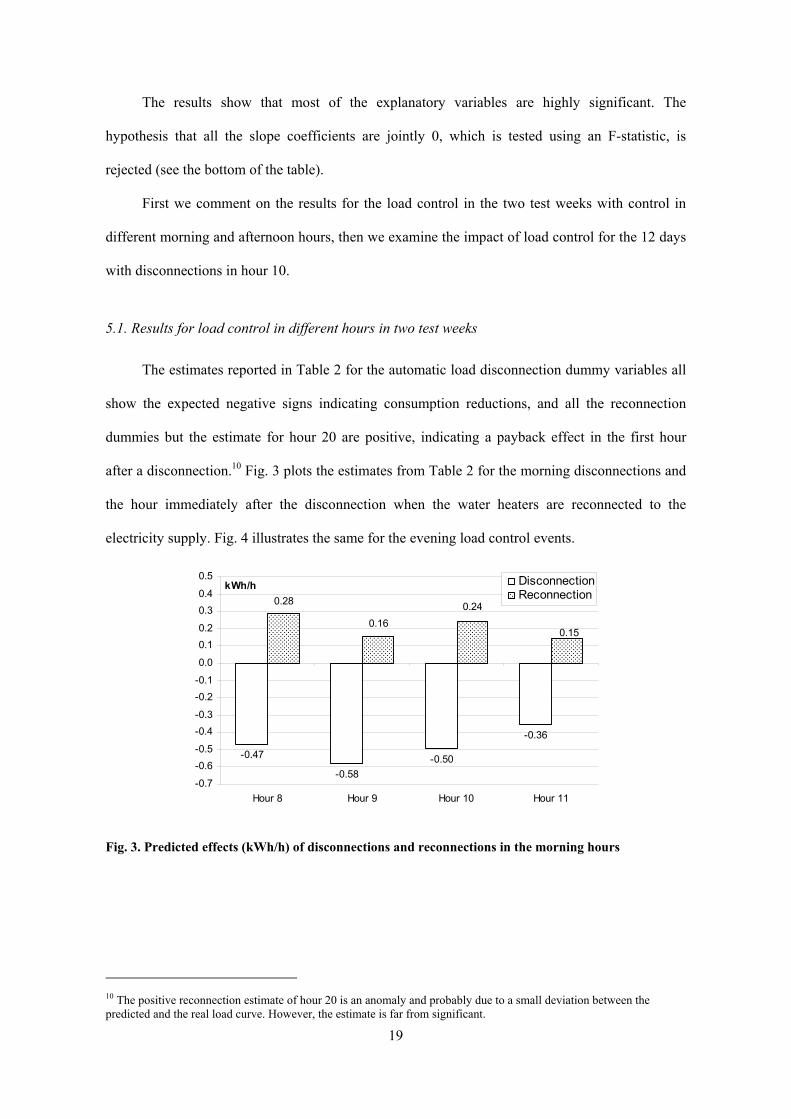
The estimates reported in Table 2 for the automatic load disconnection dummy variables all

show the expected negative signs indicating consumption reductions, and all the reconnection

dummies but the estimate for hour 20 are positive, indicating a payback effect in the first hour

after a disconnection.10 Fig. 3 plots the estimates from Table 2 for the morning disconnections and

the hour immediately after the disconnection when the water heaters are reconnected to the

electricity supply. Fig. 4 illustrates the same for the evening load control events.

-0.47

-0.58-0.50

-0.36

0.28

0.160.24

0.15

-0.7

-0.6-0.5

-0.4-0.3

-0.2-0.1

0.0

0.10.2

0.30.4

0.5

Hour 8 Hour 9 Hour 10 Hour 11

kWh/h DisconnectionReconnection

Fig. 3. Predicted effects (kWh/h) of disconnections and reconnections in the morning hours

10 The positive reconnection estimate of hour 20 is an anomaly and probably due to a small deviation between the predicted and the real load curve. However, the estimate is far from significant.

20

-0.49

-0.18

0.20

-0.60

-0.41

0.13

0.24

-0.02

-0.7-0.6

-0.5-0.4

-0.3-0.2

-0.10.0

0.10.2

0.30.4

0.5

Hour 17 Hour 18 Hour 19 Hour 20

kWh/h DisconnectionReconnection

Fig. 4. Predicted effects (kWh/h) of disconnections and reconnections in the evening hours

Our findings suggest that when a common signal for automatic disconnection of the water

heaters is sent, one can anticipate an average load reduction of between 0.36 and 0.58 kWh/h per

household for the morning hours, depending on the hour, and between 0.18 and 0.60 kWh/h in the

afternoon, depending on which hour disconnections occur. Graabak and Feilberg (2004), analysing

the impact of load control in one of the test weeks, found similar, but somewhat smaller effects.11

Our results show that disconnection in hour 9 in the morning and in hour 19 in the evening give

the largest load reductions.

Assuming an average load reduction per customer of 0.5 kWh/h, the total load reducing

potential in Norway from this measure can be inferred. Given that half of the Norwegian

households (approximately 1 million) have their water heaters disconnected, and assuming 20%

losses in the grid in a peak load situation, the potential is 0.5 kWh/h * 1,000,000 * 1.2 = 600

MWh/h reduction of load for the whole Norwegian system (assumptions correspond to those used

by Graabak and Feilberg, 2004). For comparison, the maximum measured load in Norway is

23,054 MWh/h in hour 10, 5 February 2001. This suggests that consumption could be lowered to

22,454 MWh/h this hour.

11 The differences between their results and ours may be due to different analysis methods (they compared load curves with those of a reference group) and they studied only one of the two test weeks.

21

The positive coefficients for the hour following a reconnection of the water heaters indicate

the size of the payback effect, i.e., the electricity use that will be added to the system load curve

after load control has occurred. We see that disconnections lead to surplus consumption of

between 0.15 and 0.28 kWh/h in the morning and between 012 and 0.24 kWh/h in the evening,

when the heaters are reconnected.13 Assuming the payback effect to be 0.24 kWh/h, the aggregated

extra average demand for the Norwegian system can be inferred using a similar calculation to the

above; 288 MWh/h for the first hour after the disconnection in hour 10. Imposing this value into

the same day as above suggests that consumption could increase from 22,940 MWh/h (the load in

hour 11 in the Norwegian system 5 February 2001) to approximately 23,230 MWh/h, that is, to a

higher level than the previous peak.

To illustrate how the automatic load control may affect the daily load curve for the

households in this study, Fig. 5 shows the predicted mean hourly electricity use for one of the test

days with disconnection in hour 8 and in hour 17. The payback effect is only indicated for the first

hour following a disconnection.

1.5

1.9

2.3

2.7

3.1

1 2 3 4 5 6 7 8 9 10 11 12 13 14 15 16 17 18 19 20 21 22 23 24Hour

kWh/h

With disconnectionsWithout disconnections

Fig. 5. Predicted consumption for one day with disconnection in hour 8 and 17, with and without pre-

dicted disconnection and reconnection terms

12 Assuming the negative estimate of –0.017 is not logical. It is likely to be at least 0. 13 Graabak and Feilberg (2004) found payback effects of between 0.09 and 0.29 kWh/h for the morning hours, and between 0.06 and 0.37 kWh/h for the evening hours.

22

As shown in Fig. 5, disconnections cause significant reductions in consumption. In addition,

the post-peak in the hour after the water heaters have been reconnected is evident.

5.2. Results for load control in hour 10 in twelve test days

Section 2 indicates that the size of the post-peak is likely to be largest in the first minutes

after reconnection and then diminish. However, since our data are measured with an hourly

sampling frequency, we only know the average effects over hourly intervals and not the

instantaneous power demand at the moment the heaters are reconnected, or the following

evolvement of the payback effect. Nevertheless, we know the likely range for the instantaneous

power demand. Since most heaters in Norway have heating elements with rated capacities of 2

kW, the maximum possible average payback demand at reconnection is likely not to be higher

than 2 kW. In addition, using hour 10 as an example, we know from the estimated hourly average

payback demand for the first hour after a disconnection, that the additional power demand is not

likely to be less than 0.239 kW.

However, our estimates for the five hours after the hour 10 disconnections allow us to

indicate the payback size at the time of reconnection. From Table 2 we can see that the hourly

payback is highest in the first hour and diminishes over the following hours. The estimates for the

fourth and fifth hours are not significantly different from 0. We can then anticipate that it will take

at least three hours before all energy is restored, on average, in all the water heaters affected by the

disconnection. This supports our description in Section 2 regarding the distribution of the time the

water heaters use to restore the energy in the tanks; some heaters use a short time to recover from

an energy loss, whereas others require a longer time.

We indicate a possible real-time power demand curve after reconnection by plotting the

estimates for four hours after reconnection and fitting a simple exponential trend line to the hourly

estimates (the fifth hour is excluded as it is highly insignificant). The intersection with the y-axis

for the trend line will indicate the size of the instantaneous water heater demand at the moment of

reconnection. There is a high degree of uncertainty related to this curve and its intersection, so one

must be cautious about transferring our results from the hour 10 disconnections to other hours of

23

the day or to other customer areas. Nonetheless, it is useful as a starting point for discussion and as

an illustration of how the real payback demand curve may look. In addition, bear in mind that we

use averaged data for 12 days to indicate the instantaneous payback effect, which makes it likely

that some of these 12 days experienced higher instantaneous peaks.

Fig. 6 illustrates the hourly averaged estimates for the subsequent four hours after a

disconnection and the fitted line suggests the real-time payback power demand.

0.24

0.10

0.050.02

0.0

0.1

0.2

0.3

0.4

0.5

Rc hour 10+1 Rc hour 10+2 Rc hour 10+3 Rc hour 10+4

kWh/h,kW

Averaged hourlypayback demandPossible real-timepayback demand

Fig. 6. Estimated average payback consumption for four hours following a disconnection, and a fitted

exponential trend curve, the potential real-time payback power demand

Using the four estimates to fit the exponential trend line, we find the power demand at the

time of reconnection to be approximately 0.36 kW.14 By visual inspection, the area (i.e., the energy

use) under the trend line for each hour is quite similar to the area under the hourly estimates. This

indicates that the trend line is sensible.

In the literature, the payback effect has been described using data from actual field tests and

by simulation models. For example, Bische and Sella (1985) found that a load shedding of 25 MW

of water heaters can build up to an initial payback demand of 80–90 MW. Another example is

found in Lee and Wilkins (1983). Using their model, water heater electricity consumption 15

minutes after a one-hour disconnection would be nearly twice the size that would have occurred if

14 Using only the three estimates that are significant at the 10% level, we find it to be 0.35 kW, and if all five estimates are used, the intersection is at 0.57 kW.

24

no load control had been applied, and three times the size after a two-hour disconnection.15 The

plots in Reed et al. (1989) indicate that the percentage of water heaters operating can be

approximately 2.5 times higher immediately after a two-hour disconnection than if no

disconnection is applied. In Ryan et al. (1989), the payback effect is approximately three to four

times higher than the normal water heater load, after a four-hour disconnection.

Compared with the instantaneous power demand at the moment of reconnection found in

this literature, our indication of the water heater power demand immediately after a reconnection

seems to be quite low. The size of the payback demand found is approximately 0.7 times higher

than during normal operation, while the examples from the literature range from two to four times

higher.16 One reason may be that the rated power of the heating elements in water heaters used in

experiments abroad is higher than in Norway. For example, heating elements with rated power of

4.5 kW are common in the USA (Orphelin and Adnot, 1999). Norwegian households, which

usually have 2 kW heating elements, will then have comparably lower instantaneous power

demand and longer recovering periods for the same amount of hot water use. Another reason is

probably that some of the disconnections referred to have a longer disconnection period.

Whether payback effects due to load control of residential water heaters induce new so-

called post-peaks in the electricity system higher than the targeted peak depends on the total load

in the system. If the total load curve has a pattern such that the load is low enough in the same

period as the post-peak appears, it may offset the payback effect. However, this may vary from day

to day, depending on a number of variables, as, for example, temperature. A strategy to control the

payback effect is to divide the heaters into groups and cycle the control events between the groups,

i.e., disconnect and reconnect the groups at different times during the control period. The principle

is that when some heaters are reconnected, others will be allowed to recover. By disconnecting one

or more groups of heaters when the system load reaches a pre-defined level and reconnecting on a

first-off first-on basis when the load is sufficiently low again, load reductions can be achieved

15 Displaced energy during disconnection is assumed to be 0.5 kWh/h. 16 The value 0.7 is found by dividing the power demand (0.36 kW) by the disconnected demand (0.5 kWh/h) for hour 10 (assuming the water heater power demand to be a constant 0.5 kW).

25

while a critical post-peak can be avoided (van Tonder and Lane, 1996; see also Bische and Sella

(1985), Lee and Wilkins (1983), Rau and Graham (1979), Salehfar and Patton (1989), Weller

(1988) and Gomes et al. (1999) for descriptions of cycling strategies).

5.3 Results for temperature, wind and daylight

From the other results shown in Table 2 we first see the importance of controlling for the

current and moving average temperature, as the estimates are highly significant. There is a

decreasing impact from a temperature change on electricity consumption for the current term when

temperature falls. The moving average of temperature influences consumption only linearly

because the squared term is insignificant. Second, the wind speed coefficients are highly

significant, indicating that increased wind speed increases energy use, as expected. Third, the

estimates attached to the hours of daylight variables are negative, which indicates that more

daylight reduces electricity consumption, as expected. Fourth, the price coefficient indicates that a

price increase of 0.01 NOK/kWh will decrease consumption by 0.003 kWh/h.

6. Conclusions

Estimates of the impact of load reduction indicate that direct load control of households’

water heaters can be an effective tool in decreasing peak load consumption. Disconnection of the

heaters from the electricity grid for the sample of households analyzed in this paper can be

expected to give an average reduction in load per household of between 0.36 kWh/h and 0.58

kWh/h in the morning hours and between 0.18 kWh/h and 0.60 kWh/h in the evening hours. As

described in this paper, the interruption of the natural diversity of the water heater electricity

consumption during a disconnection gives rise to a payback effect, which leads to an additional

consumption in a period after reconnection. For the first hour after a reconnection we found that

the average extra consumption can reach up to 0.28 kWh/h per household. Note that the data are

measured on an hourly sampling frequency, and that the instantaneous demand at the instant of

reconnection is likely to be higher than the hourly estimates of the payback effect. By using the

26

hourly payback demand estimates for the subsequent hours after disconnection in hour 10, we

have indicated an average power demand per household at the instant of reconnection to be 0.36

kW more than it would be if no load control had been applied. This payback demand may have the

adverse consequence of causing a new peak in the system, which suggests it may be necessary to

re-establish the diversity of the loads in a controlled manner by cycling the control events.

References

Al-Zayer, J., Al-Ibrahim, A.A., 1996. Modelling the impact of temperature on electricity

consumption in the eastern province of Saudi Arabia. Journal of Forecasting 15, 97–106.

Bische, R.F., Sella, R.A., 1985. Design and controlled use of water heater load management. IEEE

Transactions on Power Apparatus and Systems PAS–104 (6), 1290–1293.

Bye, T., Hope, E., 2005. Deregulation of electricity markets. The Norwegian experience.

Economic and Political Weekly. December 10, 5269–5278.

Charles River Associates, 2003. DM programs for Integral Energy, Final report.

Glende, I., Tellefsen T., Walther, B., 2005. Norwegian system operation facing a tight capacity

balance and severe supply conditions in dry years. www.statnett.no.

Gomes, A., Martines, A.G., Figueiredo, R., 1999. Simulation-based assessment of electrical load

management programs. International Journal of Energy Research 23, 169–181.

Gould, W., 2001. Interpreting the intercept in the fixed-effects model.

http://www.stata.com/support/faqs/stat/xtreg2.html.

Graabak, I., Feilberg, N., 2004. Forbrukerfleksibilitet ved effektiv bruk av IKT. Analyseresultater.

SINTEF, TR A5980. (In Norwegian).

Granger, C.W.J., Engle, R., Ramanathan, R., Andersen, A., 1979. Residential load curves and

time-of-day pricing: An econometric analysis. Journal of Econometrics 9 (1), 13–32.

Gustavson, M.W., Baylor, J.S., Epstein, G., 1993. Direct water heater load control – estimating

program effectiveness using an engineer model. IEEE Transactions on Power systems 8

(1), 137–143.

27

Harvey, A., Koopman, S.J., 1993. Forecasting hourly electricity demand using time-differentiated

splines. Journal of the American Statistical Association 88 (424), 1228–1336.

Hendricks, W., Koenker, R., Poirier, D.J., 1979. Residential demand for electricity. An

Econometric Approach. Journal of Econometrics 9 (1), 33–57.

Henley, A., Peirson, J., 1997. Non-linearities in electricity demand and temperature: parametric

versus non-parametric methods. Oxford Bulletin of Economics and Statistics 59 (1), 149–

161.

Henley A, Peirson, J., 1998. Residential energy demand and the interaction of price and

temperature: British experimental evidence. Journal of Energy Economics 20 (2), 157–171.

Hsiao, C., 2003. Analysis of panel data, 2nd ed. Cambridge University Press, Cambridge.

HiO (Høgskolen i Oslo), 2005. Testrapport. Måling av varmetap fra varmtvannsberedere. Rapport

nr. OIH 15091–2005.1.B. Oslo. (In Norwegian).

Johnsen, T.A., 2001. Demand, generation, and price in the Norwegian market for electric power.

Energy Economics 23, 227–251.

King, C., 2004. Integrating residential dynamic pricing and load control: The literature.

EnergyPulse. www.energypulse.net.

Larsen, M.B., Nesbakken, R, 2005. Formålsfordeling av husholdningenes elektrisitetsforbruk i

2001. Sammenligning av formålsfordelingen i 1990 og 2001, Rapport 2005/18, Statistics

Norway. (In Norwegian).

Lee, S.H., Wilkins, C.L., 1983. A practical approach to appliance load control analysis: a water

heater case study. IEEE Transactions on Power Apparatus and Systems PAS–102 (4),

1007–1013.

Malemezian, E., 2004. Largest 2-Way, direct load control program? Association of Energy

Services Professionals Member Newsletter, January.

Mills, F.A., 1995. Heat and Mass Transfer. Chicago: Richard D. Irwing, INC.

Orphelin, M., Adnot, J., 1999. Improvement of methods for reconstructing water heating

aggregated load curves and evaluating demand-side control benefits. IEEE Transactions on

Power Systems 14 (4), 1549–1555.

28

Pardo, A., Meneu, V., Valor, E., 2002. Temperature and seasonality influence on Spanish

electricity load. Energy Economics 24, 55–70.

Pettersen, T.E., 2006. Vår daglige dusj. Dagbladet, Magasinet, 14 January, 42–45. (In Norwegian).

Ramanathan, R., Engle, R., Granger, C.W.J., Vahid-Araghi, F., Bracey, C., 1997. Short-run

forecasts of electricity loads and peaks. International Journal of Forecasting 13, 161–174.

Rau, N.S., Graham, R.W., 1979. Analysis and simulation of the effects of controlled water heaters

in a winter peaking system. IEEE Transactions on Power Apparatus and Systems PAS-98

(2), 458–464.

Reed, J.H., Thompson, J.C., Broadwater, R.P., Chandrasekaran, A., 1989. Analysis of water heater

data from Athens load control experiment. IEEE transactions on Power Delivery 4 (2),

1232–1238.

Ryan, N.E., Braithwait, S.D., Powers, J.T., Smith, B.A., 1989. Generalizing direct load control

program analysis: implementation of the duty cycle approach. IEEE Transactions on Power

Systems 4 (1), 293–299.

Salehfar, H., Patton, A.D., 1989. Modeling and evaluation of the system reliability effects of direct

load control. IEEE Transactions on Power Systems 4 (3), 1024–1030.

SINTEF, 1996. Enøk i bygninger. Effektiv energibruk. Oslo: Universitetsforlaget AS. (In

Norwegian).

StataCorp, 2005. Stata Statistical Software: Release 9. StataCorp LP, College Station, TX.

Vaage, O.F., 2002. Til alle døgnets tider. Tidsbruk 1971–2000. Statistical Analyses. Statistics

Norway. (In Norwegian).

van Tonder, J.C., Lane, I.E., 1996. A load model to support demand management decisions on

domestic storage water heater control strategy. IEEE Transactions on Power Systems 11

(4), 1844–1849.

Weller, G.H., 1988. Managing the instantaneous load shape impacts caused by the operation of a

large-scale direct load control system. IEEE Transactions on Power Systems 3 (1), 197–

199.

29

Xcel Energy, 2005. www.xcelenergy.com/XLWEB/CDA/0,3080,1–1–2_738_23162–212–

11_192_352–0,00.html and http://tdworld.com/ar/power_xcel_energys_savers.

30

Appendix

Table A1. Results from the fixed effects regression

Coefficient Variable Explanation Estimate t-value p-valueδDc,8 Dc8 Dummy, disconnection, hour 8 –0.466 –14.62 0.000δDc,9 Dc9 Dummy, disconnection, hour 9 –0.580 –18.69 0.000δDc,10 Dc10 Dummy, disconnection, hour 10 –0.497 –33.91 0.000δDc,11 Dc11 Dummy, disconnection, hour 11 –0.355 –10.70 0.000δDc,17 Dc17 Dummy, disconnection, hour 17 –0.414 –11.57 0.000δDc,18 Dc18 Dummy, disconnection, hour 18 –0.489 –14.00 0.000δDc,19 Dc19 Dummy, disconnection, hour 19 –0.596 –17.85 0.000δDc,20 Dc20 Dummy, disconnection, hour 20 –0.178 –4.47 0.000δRc,8+1 Rc8+1 Dummy, reconnection, hour 8+1 0.284 7.23 0.000δRc,9+1 Rc9+1 Dummy, reconnection, hour 9+1 0.158 4.12 0.000δRc,10+1 Rc10+1 Dummy, reconnection, hour 10+1 0.239 13.60 0.000δRc,10+2 Rc10+2 Dummy, reconnection, hour 10+2 0.097 5.48 0.000δRc,10+3 Rc10+3 Dummy, reconnection, hour 10+3 0.045 2.61 0.009δRc,10+4 Rc10+4 Dummy, reconnection, hour 10+4 0.019 1.12 0.262δRc,10+5 Rc10+5 Dummy, reconnection, hour 10+5 0.002 0.10 0.918δRc,11+1 Rc11+1 Dummy, reconnection, hour 11+1 0.147 3.78 0.000δRc,17+1 Rc17+1 Dummy, reconnection, hour 17+1 0.240 5.80 0.000δRc,18+1 Rc18+1 Dummy, reconnection, hour 18+1 0.196 4.83 0.000δRc,19+1 Rc19+1 Dummy, reconnection, hour 19+1 0.134 3.14 0.002δRc,20+1 Rc20+1 Dummy, reconnection, hour 20+1 –0.017 –0.41 0.679βp p Price –0.246 –9.23 0.000βT

T Temperature –0.024 –65.18 0.000βT

2 T2 Temperature, squared –0.001 –25.22 0.000βTMA TMA Temperature, moving average –0.043 –101.74 0.000

βTMA2 TMA2 Temperature, moving average,

squared 0.000 0.38 0.706

βW W Wind 0.014 11.03 0.000βWMA

WMA Wind, moving average 0.069 31.59 0.000βdl,nov Dnov dl Daylight: November –0.072 –10.75 0.000βdl,dec Ddec dl Daylight: December –0.043 –6.83 0.000βdl,jan Djan dl Daylight: January –0.084 –13.20 0.000βdl,feb Dfeb dl Daylight: February –0.147 –25.72 0.000βdl,mar Dmar dl Daylight: March –0.128 –24.97 0.000βdl,apr Dapr dl Daylight: April –0.056 –10.57 0.000

31

Table A1. (continued)

Coefficient Variable Explanation Estimate t-value p-valueβwd,2 Dwd,2 Dummy, weekday, hour 2 –0.138 –23.67 0.000βwd,3 Dwd,3 Dummy, weekday, hour 3 –0.191 –33.32 0.000βwd,4 Dwd,4 Dummy, weekday, hour 4 –0.195 –34.29 0.000βwd,5 Dwd,5 Dummy, weekday, hour 5 –0.175 –30.63 0.000βwd,6 Dwd,6 Dummy, weekday, hour 6 –0.073 –12.49 0.000βwd,7 Dwd,7 Dummy, weekday, hour 7 0.163 26.21 0.000βwd,8 Dwd,8 Dummy, weekday, hour 8 0.477 70.06 0.000βwd,9 Dwd,9 Dummy, weekday, hour 9 0.538 75.55 0.000βwd,10 Dwd,10 Dummy, weekday, hour 10 0.505 64.08 0.000βwd,11 Dwd,11 Dummy, weekday, hour 11 0.429 54.08 0.000βwd,12 Dwd,12 Dummy, weekday, hour 12 0.374 47.27 0.000βwd,13 Dwd,13 Dummy, weekday, hour 13 0.308 39.31 0.000βwd,14 Dwd,14 Dummy, weekday, hour 14 0.286 36.57 0.000βwd,15 Dwd,15 Dummy, weekday, hour 15 0.343 43.36 0.000βwd,16 Dwd,16 Dummy, weekday, hour 16 0.458 61.53 0.000βwd,17 Dwd,17 Dummy, weekday, hour 17 0.617 86.13 0.000βwd,18 Dwd,18 Dummy, weekday, hour 18 0.699 98.69 0.000βwd,19 Dwd,19 Dummy, weekday, hour 19 0.708 101.48 0.000βwd,20 Dwd,20 Dummy, weekday, hour 20 0.707 102.31 0.000βwd,21 Dwd,21 Dummy, weekday, hour 21 0.685 102.03 0.000βwd,22 Dwd,22 Dummy, weekday, hour 22 0.627 95.62 0.000βwd,23 Dwd,23 Dummy, weekday, hour 23 0.473 74.43 0.000βwd,24 Dwd,24 Dummy, weekday, hour 24 0.240 38.62 0.000βwe,2 Dwe,2 Dummy, weekend, hour 2 –0.143 –17.10 0.000βwe,3 Dwe,3 Dummy, weekend, hour 3 –0.214 –26.01 0.000βwe,4 Dwe,4 Dummy, weekend, hour 4 –0.247 –30.42 0.000βwe,5 Dwe,5 Dummy, weekend, hour 5 –0.257 –31.86 0.000βwe,6 Dwe,6 Dummy, weekend, hour 6 –0.229 –28.31 0.000βwe,7 Dwe,7 Dummy, weekend, hour 7 –0.158 –19.14 0.000βwe,8 Dwe,8 Dummy, weekend, hour 8 –0.033 –3.84 0.000βwe,9 Dwe,9 Dummy, weekend, hour 9 0.185 20.11 0.000βwe,10 Dwe,10 Dummy, weekend, hour 10 0.451 44.60 0.000βwe,11 Dwe,11 Dummy, weekend, hour 11 0.620 58.78 0.000βwe,12 Dwe,12 Dummy, weekend, hour 12 0.663 62.28 0.000βwe,13 Dwe,13 Dummy, weekend, hour 13 0.641 60.34 0.000βwe,14 Dwe,14 Dummy, weekend, hour 14 0.600 56.42 0.000βwe,15 Dwe,15 Dummy, weekend, hour 15 0.605 57.00 0.000βwe,16 Dwe,16 Dummy, weekend, hour 16 0.628 61.63 0.000βwe,17 Dwe,17 Dummy, weekend, hour 17 0.660 65.81 0.000

32

Table A1. (continued)

Coefficient Variable Explanation Estimate t-value p-valueβwe,18 Dwe,18 Dummy, weekend, hour 18 0.686 68.50 0.000βwe,19 Dwe,19 Dummy, weekend, hour 19 0.700 70.16 0.000βwe,20 Dwe,20 Dummy, weekend, hour 20 0.675 68.73 0.000βwe,21 Dwe,21 Dummy, weekend, hour 21 0.599 63.55 0.000βwe,22 Dwe,22 Dummy, weekend, hour 22 0.500 54.53 0.000βwe,23 Dwe,23 Dummy, weekend, hour 23 0.362 40.58 0.000βwe,24 Dwe,24 Dummy, weekend, hour 24 0.175 19.56 0.000βtue Dtue Dummy, Tuesday 0.013 4.06 0.000βwed Dwed Dummy, Wednesday 0.023 7.47 0.000βthu Dthu Dummy, Thursday –0.001 –0.28 0.782βfri Dfri Dummy, Friday –0.007 –2.19 0.028βsat Dsat Dummy, Saturday 0.055 6.95 0.000βsun Dsun Dummy, Sunday 0.095 12.09 0.000βdec Ddec Dummy, December 0.085 22.65 0.000βjan Djan Dummy, January 0.156 36.39 0.000βfeb Dfeb Dummy, February 0.036 8.43 0.000βmar Dmar Dummy, March –0.046 –10.43 0.000βapr Dapr Dummy, April –0.249 –48.23 0.000βHd DHd Dummy, Holiday 0.096 11.94 0.000β17nov D17nov Dummy, control day, 17 November –0.064 –5.19 0.000β18nov D18nov Dummy, control day, 18 November –0.047 –3.83 0.000β19nov D19nov Dummy, control day, 19 November 0.033 2.84 0.004β20nov D20nov Dummy, control day, 20 November 0.004 0.35 0.729β21nov D21nov Dummy, control day, 21 November 0.040 3.21 0.001β18dec D18dec Dummy, control day, 18 December 0.010 1.05 0.295β19dec D19dec Dummy, control day, 19 December 0.081 8.19 0.000β14jan D14jan Dummy, control day, 14 January –0.044 –4.28 0.000β15jan D15jan Dummy, control day, 15 January –0.115 –10.52 0.000β16jan D16jan Dummy, control day, 16 January –0.141 –11.05 0.000β15mar D15mar Dummy, control day, 15 March 0.031 2.95 0.003β16mar D16mar Dummy, control day, 16 March 0.026 2.48 0.013β17mar D17mar Dummy, control day, 17 March –0.041 –3.96 0.000β18mar D18mar Dummy, control day, 18 March –0.066 –6.22 0.000β26apr D26apr Dummy, control day, 26 April 0.084 7.03 0.000β27apr D27apr Dummy, control day, 27 April 0.151 12.89 0.000β28apr D28apr Dummy, control day, 28 April 0.030 2.61 0.009β29apr D29apr Dummy, control day, 29 April –0.060 –5.24 0.000 Constant 2.529 123.13 0.000

33

Recent publications in the series Discussion Papers

387 G. H. Bjertnæs and T. Fæhn (2004): Energy Taxation in a Small, Open Economy: Efficiency Gains under Political Restraints

388 J.K. Dagsvik and S. Strøm (2004): Sectoral Labor Supply, Choice Restrictions and Functional Form

389 B. Halvorsen (2004): Effects of norms, warm-glow and time use on household recycling

390 I. Aslaksen and T. Synnestvedt (2004): Are the Dixit-Pindyck and the Arrow-Fisher-Henry-Hanemann Option Values Equivalent?

391 G. H. Bjønnes, D. Rime and H. O.Aa. Solheim (2004): Liquidity provision in the overnight foreign exchange market

392 T. Åvitsland and J. Aasness (2004): Combining CGE and microsimulation models: Effects on equality of VAT reforms

393 M. Greaker and Eirik. Sagen (2004): Explaining experience curves for LNG liquefaction costs: Competition matter more than learning

394 K. Telle, I. Aslaksen and T. Synnestvedt (2004): "It pays to be green" - a premature conclusion?

395 T. Harding, H. O. Aa. Solheim and A. Benedictow (2004). House ownership and taxes

396 E. Holmøy and B. Strøm (2004): The Social Cost of Government Spending in an Economy with Large Tax Distortions: A CGE Decomposition for Norway

397 T. Hægeland, O. Raaum and K.G. Salvanes (2004): Pupil achievement, school resources and family background

398 I. Aslaksen, B. Natvig and I. Nordal (2004): Environmental risk and the precautionary principle: “Late lessons from early warnings” applied to genetically modified plants

399 J. Møen (2004): When subsidized R&D-firms fail, do they still stimulate growth? Tracing knowledge by following employees across firms

400 B. Halvorsen and Runa Nesbakken (2004): Accounting for differences in choice opportunities in analyses of energy expenditure data

401 T.J. Klette and A. Raknerud (2004): Heterogeneity, productivity and selection: An empirical study of Norwegian manufacturing firms

402 R. Aaberge (2005): Asymptotic Distribution Theory of Empirical Rank-dependent Measures of Inequality

403 F.R. Aune, S. Kverndokk, L. Lindholt and K.E. Rosendahl (2005): Profitability of different instruments in international climate policies

404 Z. Jia (2005): Labor Supply of Retiring Couples and Heterogeneity in Household Decision-Making Structure

405 Z. Jia (2005): Retirement Behavior of Working Couples in Norway. A Dynamic Programming Approch

406 Z. Jia (2005): Spousal Influence on Early Retirement Behavior

407 P. Frenger (2005): The elasticity of substitution of superlative price indices

408 M. Mogstad, A. Langørgen and R. Aaberge (2005): Region-specific versus Country-specific Poverty Lines in Analysis of Poverty

409 J.K. Dagsvik (2005) Choice under Uncertainty and Bounded Rationality

410 T. Fæhn, A.G. Gómez-Plana and S. Kverndokk (2005): Can a carbon permit system reduce Spanish unemployment?

411 J. Larsson and K. Telle (2005): Consequences of the IPPC-directive’s BAT requirements for abatement costs and emissions

412 R. Aaberge, S. Bjerve and K. Doksum (2005): Modeling Concentration and Dispersion in Multiple Regression

413 E. Holmøy and K.M. Heide (2005): Is Norway immune to Dutch Disease? CGE Estimates of Sustainable Wage Growth and De-industrialisation

414 K.R. Wangen (2005): An Expenditure Based Estimate of Britain's Black Economy Revisited

415 A. Mathiassen (2005): A Statistical Model for Simple, Fast and Reliable Measurement of Poverty

416 F.R. Aune, S. Glomsrød, L. Lindholt and K.E. Rosendahl: Are high oil prices profitable for OPEC in the long run?

417 D. Fredriksen, K.M. Heide, E. Holmøy and I.F. Solli (2005): Macroeconomic effects of proposed pension reforms in Norway

418 D. Fredriksen and N.M. Stølen (2005): Effects of demographic development, labour supply and pension reforms on the future pension burden

419 A. Alstadsæter, A-S. Kolm and B. Larsen (2005): Tax Effects on Unemployment and the Choice of Educational Type

420 E. Biørn (2005): Constructing Panel Data Estimators by Aggregation: A General Moment Estimator and a Suggested Synthesis

421 J. Bjørnstad (2005): Non-Bayesian Multiple Imputation

422 H. Hungnes (2005): Identifying Structural Breaks in Cointegrated VAR Models

423 H. C. Bjørnland and H. Hungnes (2005): The commodity currency puzzle

424 F. Carlsen, B. Langset and J. Rattsø (2005): The relationship between firm mobility and tax level: Empirical evidence of fiscal competition between local governments

425 T. Harding and J. Rattsø (2005): The barrier model of productivity growth: South Africa

426 E. Holmøy (2005): The Anatomy of Electricity Demand: A CGE Decomposition for Norway

427 T.K.M. Beatty, E. Røed Larsen and D.E. Sommervoll (2005): Measuring the Price of Housing Consumption for Owners in the CPI

428 E. Røed Larsen (2005): Distributional Effects of Environmental Taxes on Transportation: Evidence from Engel Curves in the United States

429 P. Boug, Å. Cappelen and T. Eika (2005): Exchange Rate Rass-through in a Small Open Economy: The Importance of the Distribution Sector

430 K. Gabrielsen, T. Bye and F.R. Aune (2005): Climate change- lower electricity prices and increasing demand. An application to the Nordic Countries

431 J.K. Dagsvik, S. Strøm and Z. Jia: Utility of Income as a Random Function: Behavioral Characterization and Empirical Evidence

432 G.H. Bjertnæs (2005): Avioding Adverse Employment Effects from Energy Taxation: What does it cost?

3

433. T. Bye and E. Hope (2005): Deregulation of electricity markets—The Norwegian experience

434 P.J. Lambert and T.O. Thoresen (2005): Base independence in the analysis of tax policy effects: with an application to Norway 1992-2004

435 M. Rege, K. Telle and M. Votruba (2005): The Effect of Plant Downsizing on Disability Pension Utilization

436 J. Hovi and B. Holtsmark (2005): Cap-and-Trade or Carbon Taxes? The Effects of Non-Compliance and the Feasibility of Enforcement

437 R. Aaberge, S. Bjerve and K. Doksum (2005): Decomposition of Rank-Dependent Measures of Inequality by Subgroups

438 B. Holtsmark (2005): Global per capita CO2 emissions - stable in the long run?

439 E. Halvorsen and T.O. Thoresen (2005): The relationship between altruism and equal sharing. Evidence from inter vivos transfer behavior

440 L-C. Zhang and I. Thomsen (2005): A prediction approach to sampling design

441 Ø.A. Nilsen, A. Raknerud, M. Rybalka and T. Skjerpen (2005): Lumpy Investments, Factor Adjustments and Productivity

442 R. Golombek and A. Raknerud (2005): Exit Dynamics with Adjustment Costs

443 G. Liu, T. Skjerpen, A. Rygh Swensen and K. Telle (2006): Unit Roots, Polynomial Transformations and the Environmental Kuznets Curve

444 G. Liu (2006): A Behavioral Model of Work-trip Mode Choice in Shanghai

445 E. Lund Sagen and M. Tsygankova (2006): Russian Natural Gas Exports to Europe. Effects of Russian gas market reforms and the rising market power of Gazprom

446 T. Ericson (2006): Households' self-selection of a dynamic electricity tariff

447 G. Liu (2006): A causality analysis on GDP and air emissions in Norway

448 M. Greaker and K.E. Rosendahl (2006): Strategic Climate Policy in Small, Open Economies

449 R. Aaberge, U. Colombino and T. Wennemo (2006): Evaluating Alternative Representation of the Choice Sets in Models of Labour Supply

450 T. Kornstad and T.O. Thoresen (2006): Effects of Family Policy Reforms in Norway. Results from a Joint Labor Supply and Child Care Choice Microsimulation Analysis

451 P. Frenger (2006): The substitution bias of the consumer price index

452 B. Halvorsen (2006): When can micro properties be used to predict aggregate demand?

453 J.K. Dagsvik, T. Korntad and T. Skjerpen (2006): Analysis of the disgouraged worker phenomenon. Evidence from micro data

454 G. Liu (2006): On Nash equilibrium in prices in an oligopolistic market with demand characterized by a nested multinomial logit model and multiproduct firm as nest

455 F. Schroyen and J. Aasness (2006): Marginal indirect tax reform analysis with merit good arguments and environmental concerns: Norway, 1999

456 L-C Zhang (2006): On some common practices of systematic sampling

457 Å. Cappelen (2006): Differences in Learning and Inequality

458 T. Borgersen, D.E. Sommervoll and T. Wennemo (2006): Endogenous Housing Market Cycles

459 G.H. Bjertnæs (2006): Income Taxation, Tuition Subsidies, and Choice of Occupation

460 P. Boug, Å. Cappelen and A.R. Swensen (2006): The New Keynesian Phillips Curve for a Small Open Economy

461 T. Ericson (2006): Time-differentiated pricing and direct load control of residential electricity consumption

462 T. Bye, E. Holmøy and K. M. Heide (2006): Removing policy based comparative advantage for energy intensive production. Necessary adjustments of the real exchange rate and industry structure

463 R. Bjørnstad and R. Nymoen (2006): Will it float? The New Keynesian Phillips curve tested on OECD panel data

464 K.M.Heide, E. Holmøy, I. F. Solli and B. Strøm (2006): A welfare state funded by nature and OPEC. A guided tour on Norway's path from an exceptionally impressive to an exceptionally strained fiscal position

465 J.K. Dagsvik (2006): Axiomatization of Stochastic Models for Choice under Uncertainty

466 S. Hol (2006): The influence of the business cycle on bankruptcy probability

467 E. Røed Larsen and D.E. Sommervoll (2006): The Impact on Rent from Tenant and Landlord Characteristics and Interaction

468 Suzan Hol and Nico van der Wijst (2006): The financing structure of non-listed firms

469 Suzan Hol (2006): Determinants of long-term interest rates in the Scandinavian countries

470 R. Bjørnstad and K. Øren Kalstad (2006): Increased Price Markup from Union Coordination - OECD Panel Evidence.

471 E. Holmøy (2006): Real appreciation as an automatic channel for redistribution of increased government non-tax revenue.

472 T. Bye, A. Bruvoll and F.R. Aune (2006): The importance of volatility in inflow in a deregulated hydro-dominated power market.

473 T. Bye, A. Bruvoll and J. Larsson (2006): Capacity utilization in a generlized Malmquist index including environmental factors: A decomposition analysis

474 A. Alstadsæter (2006): The Achilles Heel of the Dual Income Tax. The Norwegian Case

475 R. Aaberge and U. Colombino (2006): Designing Optimal Taxes with a Microeconometric Model of Household Labour Supply

476 I. Aslaksen and A.I. Myhr (2006): “The worth of a wildflower”: Precautionary perspectives on the environmental risk of GMOs

477 T. Fæhn and A. Bruvoll (2006): Richer and cleaner - at others’ expense?

478 K.H. Alfsen and M. Greaker (2006): From natural resources and environmental accounting to construction of indicators for sustainable development

479 T. Ericson (2006): Direct load control of residential water heaters

4