Embed Size (px)
Citation preview

Environmental Impact on Residential Load Modeling
Khaled Hamed Al-Ghamdi
Electrical Engineering
May 2003

ii
KING FAHD UNIVERSITY OF PETROLEUM AND MINERALS
DHAHRAN, SAUDI ARABIA
DEANSHIP OF GRADUATE STUDIES
This thesis, written by
KHALED HAMED ABDULLAH AL-GHAMDI
under the direction of his Thesis advisor, and approved by his Thesis Committee, has been
presented to and accepted by Dean of Graduate Studies, in partial fulfillment of the
requirements for the degree of
MASTER OF SCIENCE IN ELECTRICAL ENGINEERING
Thesis Committee:
________________________________ Dr.Chokri Belhaj Ahmed (Chairman) _________________________________ Dr.Rached Ben-Mansour (Co-Chairman) _________________________________ Dr.Ibrahim M. El-Amin (Member)
_______________________________ _________________________________ Dr.Jamil M. Bakhashwain Dr.Ibrahim O. Habiballah (Member) Department Chairman
_________________________________ Dr.Essam Z. Abdel-Aziz (Member)
_______________________________ Dr.Osama A. Jannadi Dean of Graduate Studies
Date: ______________________

iii
بسم اهللا الرحمن الرحيم
أهــــــداء
جنات أسأل اهللا ان يرحمه ويجمعني به في-إلي والدي العزيز .الخلد
أسأل اهللا ان ُيحسن خاتمتها ويرزقها -ةوإلي والدتي العزيز .االعلـى الفردوس
التي كانت عوناً لي بـعد اهللا، وكانت -ةوإلي زوجتي الغالي . السراِء والضراء معي في
أسأل اهللا أن يجـعلهم - تركي وروانأوالديوإلي قرة عيني . صالحين أبـناًء
. تيوإلي من اُحب أخواني و أخوا

iv
Acknowledgement
Acknowledgment is due to King Fahd University of Petroleum and Minerals for providing
support for this work.
I wish to express my deep appreciation to Dr.Chokri Belhaj Ahmed, who served as my
major advisor, for his guidance and invaluable suggestions through the course of this
work. I also wish to thank the other members of my Thesis Committee Dr.Rached Ben-
Mansour, Dr.Ibrahim El-Amin, Dr.Ibrahim Habiballah and Dr.Essam Abdel-Aziz for their
cooperation, encouragement and help. Thanks are also due to Electrical Engineering
Department Chairman, Dr.Jamil Bakhashwain and other faculty members for their interest
and support.
Thanks are also due to the Saudi Electricity Company-Eastern Region Branch and all its
staff members who provided me with the information needed for this work.
Special thanks are due to my parents who took care of me and instilled in me the self-
dependence, to my wife who was very patient in encouraging me to complete this work,
and to all family members for their support.

v
Contents
Acknowledgement iv
List of Tables viii
List of Figures x
Abstract (English) xv
Abstract (Arabic) xvi
1. INTRODUCTION 1 2. LITERATURE REVIEW 5 3. LOAD MODELING CONCEPTS AND APPROACH 10
3.1 Basic Load Modeling Concepts…………………………………….. 10 3.2 Load Model Theory…………………………………………………. 16 3.3 Load Model Derivation……………………………………………... 17 3.4 Load Model Parameter Estimation………………………………….. 26
vi
4. PROBLEM DEFINITION AND OBJECTIVE 28
4.1 Problem Definition………………………………………………….. 28 4.2 Objective……………………………………………………………. 43
5. LOAD MODEL RESULTS AND DISCUSSION 44 5.1 Parameter Estimation Method………………………………………. 44 5.2 EPRI Load Model Example………………………………………… 45 5.3 Load Modeling Structure Selection…………………………………. 50 5.4 Data For Load Modeling……………………………………………. 53
5.4.1 Basic Approaches to Obtain Data…………………………... 53
5.4.2 Data Selected……………………………………………….. 55
5.5 Load Model Development Steps……………………………………. 56 5.6 Formulated Load Model…………………………………………….. 58
5.6.1 Residential Load Model for June………………………….... 58 5.6.2 Residential Load Model for July ………………………….... 61 5.6.3 Residential Load Model for August……………………….... 61 5.6.4 Residential Load Model for September...………………....... 66
5.7 Statistical Error Analysis …………………………………………… 69
5.8 Forecasting Hourly Residential Load Demand..……………………. 82
5.8.1 Utility Current Approach…………………………………… 82 5.8.2 Weather Related Approach…………………………………. 83
5.9 Test Load Model With New Substation ……………………………. 87
vii
6. CONCLUSIONS AND RECOMMENDATIONS 96
6.1 Conclusions…………………………………………………………. 96 6.2 Recommendations…………………………………………………... 98
APPENDICES 99
A Load Modeling Structure Selection…………………………………. 100 B Data For Load Modeling……………………………………………. 112
B.1 Original Raw Data …………………………………………… 113 B.2 Data For Load Modeling……………………………………… 124
C Error Bars Plots……………………………………………………... 140
BIBLIOGRAPHY 197 Vita 200
viii
List of Tables
3.1 Comparison Among Load Parameters of Various Kinds of Typical System Load…………………………………………………….….. 23
4.1 Load Data of AGRABIA Substation 1st August 2000……………………… 29 4.2 Load Data of AGRABIA Substation 1st February 2000……………………. 32 5.1 Load Data of The Heat Pump……………………………………………….. 48 5.2 Data of Matrix X for EPRI Example………………………………………... 49 5.3 Load Model Structures for Active Power Demand…………………………. 51 5.4 Load Model Structures for Reactive Power Demand……………………….. 52 5.5 Formulated Residential Load Model for June at 2 am ……………………... 59 5.6 Formulated Residential Load Model for June at 2 pm ……………………... 60 5.7 Formulated Residential Load Model for July at 2 am ……………………... 62 5.8 Formulated Residential Load Model for July at 2 pm ……………………... 63 5.9 Formulated Residential Load Model for August at 2 am …………………... 64 5.10 Formulated Residential Load Model for August at 2 pm ………………….. 65 5.11 Formulated Residential Load Model for September at 2 am ………………. 67 5.12 Formulated Residential Load Model for September at 2 pm ………………. 68 5.13 Statistical Error analysis for June Models ………………………………….. 70 5.14 Statistical Error analysis for July Models…………………………………... 71
ix
5.15 Statistical Error analysis for August Models………………………………... 72 5.16 Statistical Error analysis for September Models……………………………. 73 A.1 Load Model Structure A (1999 August at 2 pm)…………………………… 101 A.2 Load Model Structure B (1999 August at 2 pm)…………………………… 102 A.3 Load Model Structure C (1999 August at 2 pm)…………………………… 103 A.4 Load Model Structure D (1999 August at 2 pm)…………………………… 104 A.5 Load Model Structure E (1999 August at 2 pm)…………………………… 105 A.6 Load Model Structure F (1999 August at 2 pm)…………………………… 106 A.7 Load Model Structure G (1999 August at 2 pm)…………………………… 107 A.8 Load Model Structure H (1999 August at 2 pm)…………………………… 108 A.9 Load Model Structure I (1999 August at 2 pm)…………………………… 109 A.10 Load Model Structure J (1999 August at 2 pm)…………………………… 110 A.11 Load Model Structure K (1999 August at 2 pm)…………………………… 111 B.1 Load Model Data for June 2 am…………………………………………….. 124 B.2 Load Model Data for June 2 pm…………………………………………….. 126 B.3 Load Model Data for July 2 am…………………………………………….. 128 B.4 Load Model Data for July 2 pm…………………………………………….. 130 B.5 Load Model Data for August 2 am………………………………………….. 132 B.6 Load Model Data for August 2 pm………………………………...……….. 134 B.7 Load Model Data for September 2 am……………..……………………….. 136 B.8 Load Model Data for September 2 pm……………………………..……….. 138
x
List of Figures
2.1 Power System Configuration……………………………………………….. 12 2.2 Terminology for Component-Based Load Modeling………………………. 13 3.1 EMTP (Electromagnetic Transient Program) Voltage and Frequency-
Dependent Static Loads……………………………………………………... 25 4.1 Active Power, Temperature and Humidity Vs. Hour at 1st August 2000…… 30 4.2 Reactive Power, Temperature and Humidity Vs. Hour at 1st August 2000.... 31 4.3 Active Power, Temperature and Humidity Vs. Hour at 1st February 2000…. 33 4.4 Reactive Power, Temperature and Humidity Vs. Hour at 1st February 2000 34 4.5 Power verses Temperature Summer 2001 at 2 am………………………….. 37 4.6 Power verses Temperature Summer 2001 at 10 am………………………... 38 4.7 Power verses Temperature Summer 2001 at 2 pm………………………….. 39 4.8 Power verses Temperature Summer 2001 at 11 pm………………………… 40 4.9 Power verses Temperature Winter 2001 at 2 am………….………………... 41 4.10 Power verses Temperature Winter 2001 at 2 pm…………………………… 42 5.1 Space Heating Heat Pump Characteristics ……………….………………... 46 5.2 Residential Load Model Development Steps ….…….……………….......... 57 5.3 Error Bar for the Active Power Model for 1998 August at 2 pm.…………. 74 5.4 Error Bar for the Active Power Model for 1999 August at 2 pm.…………. 75
xi
5.5 Error Bar for the Active Power Model for 2000 August at 2 pm.…………. 76 5.6 Error Bar for the Active Power Model for 2001 August at 2 pm.…………. 77 5.7 Error Bar for the Reactive Power Model for 1998 August at 2 pm.……….. 78 5.8 Error Bar for the Reactive Power Model for 1999 August at 2 pm.……….. 79 5.9 Error Bar for the Reactive Power Model for 2000 August at 2 pm.……….. 80 5.10 Error Bar for the Reactive Power Model for 2001 August at 2 pm.……….. 81 5.11 Actual and Forecasted Active Power of Agrabia Substation for 2002
August at 2 pm…………………………………………………………….. 85
5.12 Actual and Forecasted Reactive Power of Agrabia Substation for 2002
August at 2 pm…………………………………………………………….. 86
5.13 Actual and Simulated Active Power of Bayonia Substation for 2001 June
at 2 am……………………………………………………………………... 88
5.14 Actual and Simulated Reactive Power of Bayonia Substation for 2001
June at 2 am……………………………………………………………….. 89
5.15 Actual and Simulated Active Power of Bayonia Substation for 2001
August at 2 pm…………………………………………………………….. 90
5.16 Actual and Simulated Reactive Power of Bayonia Substation for 2001
August at 2 pm…………………………………………………………….. 91
5.17 Error Bar for the Active Power of Bayonia for 2001 June at 2 am………… 92 5.18 Error Bar for the Reactive Power of Bayonia for 2001 June at 2 am……… 93 5.19 Error Bar for the Active Power of Bayonia for 2001 August at 2 pm……... 94 5.20 Error Bar for the Reactive Power of Bayonia for 2001 August at 2 pm…… 95 C.1 Error Bar for the Active Power Model for 1998 June at 2 am……………... 141 C.2 Error Bar for the Reactive Power Model for 1998 June at 2 am…………… 142 C.3 Error Bar for the Active Power Model for 1998 June at 2 pm……………... 143 C.4 Error Bar for the Reactive Power Model for 1998 June at 2 pm…………… 144
xii
C.5 Error Bar for the Active Power Model for 1999 June at 2 am……………... 145 C.6 Error Bar for the Reactive Power Model for 1999 June at 2 am…………… 146 C.7 Error Bar for the Active Power Model for 1999 June at 2 pm……………... 147 C.8 Error Bar for the Reactive Power Model for 1999 June at 2 pm…………… 148 C.9 Error Bar for the Active Power Model for 2000 June at 2 am……………... 149 C.10 Error Bar for the Reactive Power Model for 2000 June at 2 am…………. 150 C.11 Error Bar for the Active Power Model for 2000 June at 2 pm……………. 151 C.12 Error Bar for the Reactive Power Model for 2000 June at 2 pm…………. 152 C.13 Error Bar for the Active Power Model for 2001 June at 2 am….………... 153 C.14 Error Bar for the Reactive Power Model for 2001 June at 2 am…………. 154 C.15 Error Bar for the Active Power Model for 2001 June at 2 pm……………. 155 C.16 Error Bar for the Reactive Power Model for 2001 June at 2 pm…………. 156 C.17 Error Bar for the Active Power Model for 1998 July at 2 am…………... 157 C.18 Error Bar for the Reactive Power Model for 1998 July at 2 am………… 158 C.19 Error Bar for the Active Power Model for 1998 July at 2 pm…………….. 159 C.20 Error Bar for the Reactive Power Model for 1998 July at 2 pm………… 160 C.21 Error Bar for the Active Power Model for 1999 July at 2 am…………... 161 C.22 Error Bar for the Reactive Power Model for 1999 July at 2 am………… 162 C.23 Error Bar for the Active Power Model for 1999 July at 2 pm…………... 163 C.24 Error Bar for the Reactive Power Model for 1999 July at 2 pm………… 164 C.25 Error Bar for the Active Power Model for 2000 July at 2 am…………... 165 C.26 Error Bar for the Reactive Power Model for 2000 July at 2 am…………. 166 C.27 Error Bar for the Active Power Model for 2000 July at 2 pm……………. 167
xiii
C.28 Error Bar for the Reactive Power Model for 2000 July at 2 pm…………. 168 C.29 Error Bar for the Active Power Model for 2001 July at 2 am….………... 169 C.30 Error Bar for the Reactive Power Model for 2001 July at 2 am…………. 170 C.31 Error Bar for the Active Power Model for 2001 July at 2 pm……………. 171 C.32 Error Bar for the Reactive Power Model for 2001 July at 2 pm…………. 172 C.33 Error Bar for the Active Power Model for 1998 August at 2 am…………. 173 C.34 Error Bar for the Reactive Power Model for 1998 August at 2 am………. 174 C.35 Error Bar for the Active Power Model for 1999 August at 2 am…………. 175 C.36 Error Bar for the Reactive Power Model for 1999 August at 2 am………. 176 C.37 Error Bar for the Active Power Model for 2000 August at 2 am…………. 177 C.38 Error Bar for the Reactive Power Model for 2000 August at 2 am………. 178 C.39 Error Bar for the Active Power Model for 2001 August at 2 am….……… 179 C.40 Error Bar for the Reactive Power Model for 2001 August at 2 am………. 180 C.41 Error Bar for the Active Power Model for 1998 September at 2 am……… 181 C.42 Error Bar for the Reactive Power Model for 1998 September at 2 am…… 182 C.43 Error Bar for the Active Power Model for 1998 September at 2 pm……... 183 C.44 Error Bar for the Reactive Power Model for 1998 September at 2 pm…… 184 C.45 Error Bar for the Active Power Model for 1999 September at 2 am……… 185 C.46 Error Bar for the Reactive Power Model for 1999 September at 2 am…… 186 C.47 Error Bar for the Active Power Model for 1999 September at 2 pm…….. 187 C.48 Error Bar for the Reactive Power Model for 1999 September at 2 pm…… 188 C.49 Error Bar for the Active Power Model for 2000 September at 2 am……… 189 C.50 Error Bar for the Reactive Power Model for 2000 September at 2 am…… 190 C.51 Error Bar for the Active Power Model for 2000 September at 2 pm…….. 191

xiv
C.52 Error Bar for the Reactive Power Model for 2000 September at 2 pm…… 192 C.53 Error Bar for the Active Power Model for 2001 September at 2 am….….. 193 C.54 Error Bar for the Reactive Power Model for 2001 September at 2 am…… 194 C.55 Error Bar for the Active Power Model for 2001 September at 2 pm…….. 195 C.56 Error Bar for the Reactive Power Model for 2001 September at 2 pm…… 196

xv
Abstract Name : Khaled Hamed Abdullah Al-Ghamdi
Title : Environmental Impact on Residential Load Modeling
Major Field : Electrical Engineering
Date of Degree : May 2003
Residential loads in Gulf area are highly affected by environmental conditions. The drastically changeable weather conditions in particular ambient temperature and relative humidity influence the residential air-conditioning demand. This thesis presents the derived mathematical form of power system loads that reflect the environmental conditions namely temperature and relative humidity. Large amount of measured data for several years (year 1998 to year 2002) have been collected. These data concern a highly hot and humid area at the eastern province in Saudi Arabia. Typical data for residential load models has been selected. The data have been selected to reflect the impact of temperature and relative humidity at steady voltage and at constant frequency. Throughout the analysis, observations and investigations of the data the sensitivity of power demand to temperature and relative humidity has shown the natural expected behavior. The derived mathematical models have shown a non-linear relation of the power demand with temperature as well with relative humidity and a coupling between temperature and humidity. These formulated Load models have been tested and validated.
MASTER OF SCIENCE DEGREE King Fahd University of Petroleum and Minerals
Dhahran, Saudi Arabia May 2003

xvi
خالصة الرسالة
الـغـامديعبدا هللاخـالد حـامد : اسم الطالب
الجوية على استهالك الطاقة السكنيةاألحوالتأثير : عنوان الرسالة
ةكهر بائيهندسة : التخصص
هـ١٤٢٤ األولربيع : تاريخ الشهادة
ومن هذه األحوال التغيير العنيف . المحيطة بهاتتأثر األحمال الكهربائية السكنية في منطقة الخليج باألحوال البيئية الطقس وخصوصاً درجة الحرارة ودرجة الرطوبة النسبية، حيث تأثر على استهالك الطاقة الكهربائية أحوالفي
.للمكيفات المنزلية
دامها في عملية تحليل واختبار أنظمة الطاقة هذة الرسالة تعرض عملية تمثيل األحمال الكهربائية التي يتم استخهذة . ٢٠٠٢ الي سنة ١٩٩٨ المعلومات من سنة القياسات ولقد تم جمع عدد هائل من. الكهربائية ودراستها
إن. المعلومات تعود الي منطقة في شرق المملكة العربية السعودية حيث تتصف بالحرارة والرطوبة العاليةستخدمة في هذا البحث تم جمعها وترتيبها بحيث تُبين تأثير األحوال الجوية على استهالك المعلومات والبيانات الم
. الطاقة الكهربائية السكنية دون وجود أي تغيير في الجهد والتردد
وقد بينت التحاليل والمالحظات أن حساسية العالقة بين درجة الحرارة ودرجة الرطوبة النسبية واستهالك الطاقة .ية، هي عالقة طبيعية، كما كان متوقعالكهربائ
أن العالقة بين درجة الحرارة ودرجة أوضحت النماذج الحسابية المشتقة الستهالك الطاقة الكهربائية السكنية إن
وقد تم اختبار هذة النماذج الحسابية، وذلك . معقدة رياضيةالرطوبة النسبية واستهالك الطاقة الكهربائية، هي عالقة . الناتجة من النموذج الحسابياالفتراضيةمقارنة األحمال األصلية مع األحمال عن طريق
درجة الماجسـتير في العلوم جامعـة المـلك فهـد للبـترول والمعـادن
الظهران ، المملكة العربية السعودية هـ١٤٢٤ ألولربيع ا: التاريخ

1
Chapter 1
INTRODUCTION The system loads have normally been represented by constant values of active and
reactive power for power flow purposes. This is adequate for most studies, but the
response of system loads to voltage variation and environmental factors are useful in some
types of analysis.
Load modeling is important for different power system studies such as steady state,
transient stability, voltage stability and small-signal stability damping studies.
Steady state studies
Most power programs, currently in use, do not have provisions for representing the
voltage sensitivity of the load, since all loads are represented as constant MVA. This is
appropriate for baseline planning studies and for the evaluation of steady-state conditions
following contingencies, when voltage regulating devices will have returned the voltage
to near its normal value. For studies of voltages and flows immediately after
contingencies, a representation of the load’s voltage sensitivity is necessary. [1]
1

2
Transient stability studies
Transient stability studies provide information on the capability of a power system to
remain in synchronism following major disturbances, such as system faults and equipment
outages. The dynamic response of system voltages, machine angles, and power flows are
computed by numerical integration of the differential equations of the system. Loads are
usually represented by static models that are sensitive to voltage and frequency changes,
but without differential equations. Dynamic induction motor models are usually available
and have been used in the past primarily for representing large industrial or power plant
auxiliary motors. [1]
Voltage stability studies
Voltage stability is influenced by nonlinear time-variant controls (e.g. generator excitation
limiters, under-load tap-changing transformers) and load characteristics (e.g. motors),
which change with both voltage level and time. The proper representation of load is
important for system stability studies. [2]
Small-signal stability studies
Inter-area modes of oscillation, involving a number of generators widely distributed over
the power system, often results in significant variations in voltage and local frequency. In
such cases, the load voltage and frequency characteristics may have a significant effect on
the damping of the oscillations. Many studies showed that using a constant impedance
load representation in small-signal analysis tend to overestimate the damping. [3]

3
Many studies have shown that load representation can have a significant impact on results
analysis. Therefore, efforts directed at improving load modeling are of major importance.
The accurate modeling of loads continues to be a difficult task due to following factors:
• The large number of diverse load components.
• The ownership and location of load devices in customer facilities not directly
accessible to the electric utility.
• Changing load composition with time of day, week and seasons.
• The lack of precise information on the composition of the load.
• The lack of accurate system tests for identifying load models. [3,4]
Electric utility analysis and their management require evidence of the benefits of
improved load representation in order to justify the effort and expense of collecting and
processing load data and, perhaps, modifying computer program load models. The
benefits of improved load representation fall into the following categories:
A. If present load representation produces overly-pessimistic results:
1. In planning studies, the benefits of improved modeling will be in deferring or
avoiding the expense of system modifications and equipment additions.
2. In operating studies, the benefits will be in increasing power transfer limits,
with resulting economic benefits.

4
B. If present load representation produces overly-optimistic results:
1. In planning studies, the benefit of improved modeling will be in avoiding
system inadequacies that may result in costly operating limitations.
2. In operating studies, the benefit may be in preventing system emergencies
resulting from overly-optimistic operating limits.
In addition, failure to represent loads in sufficient detail may produce results that miss
significant phenomena. [3]
The residential load in Saudi Arabia is mostly affected by the weather conditions
especially in summer where the temperature and the relative humidity are varying [5, 6].
Therefore, this work was initiated to provide more realistic residential load models where
the variation of active and reactive power represented as a function of the temperature and
relative humidity, in terms of the associated model parameter estimation.
This thesis is divided into six chapters as follows
• Introduction is given in chapter 1.
• Literature review is given in chapter 2.
• Load modeling concepts and approach are presented in chapter 3.
• Problem definition and objective are discussed in chapter 4.
• Chapter five presents the load modeling results and discussion.
• Conclusions and recommendations are given in chapter 6.

5
Chapter 2
LITERATURE REVIEW Aggregate load modeling is a traditional field in power system planning; however,
modeling of residential appliance loads for use in direct load control has been a concern
for only the last decade.
Because of the high cost of the installation of new generation capacity, and the high price
of oil, several utilities have attempted to use the existing generation capacity more
efficiently by applying sophisticated direct load control strategies, rather than building
new capacity. Much research is taking place in order to develop high accuracy load
models to be used by the utilities for this purpose.
In 1984, EPRI contracted with General Electric [7], under project RP849-7, “Load
Modeling for Power Flow and Transient Stability Computer Studies,” to develop
production-grade computer programs and documentation that would provide an easy way
for electric utility engineers to prepare better load models for power flow and transient
stability studies. This has been accomplished by the development of the Load Model
Synthesis (LOADSYN) computer program package, which permits the user to develop
5

6
load models for his system with a minimum amount of data on the system loads, simply
the mix of various classes, e.g., residential, commercial, industrial. Default data, which
can be easily modified by user, is provided for the composition of each class and for the
characteristics of the load components. A Load Modeling Reference Manual was written
to assist utility engineers in gathering data and applying the software.
IEEE Task Force on load representation for dynamic performance [3] summarized the
state of the art of representation of power system loads for dynamic performance analysis
purposes. It includes definition of terminology, discussion of the importance of load
modeling, important considerations for different types of analyses. Typical load model
data and methods for acquiring data are reviewed.
Dias and Hawary [8] considered the problem of estimating the parameters of static power
system load models intended for use in load flow studies that incorporate the variation of
active and reactive power with busbar voltages. A number of load model forms are
considered, where the parameters estimation task involves the iterative solution of
nonlinear equations. The use of Newton method to obtain the parameters provided is
considered to be unsatisfactory in many instances. Alternative iterative techniques such as
the BFGS (Broyden, Fletcher, Goldfarb and Shanno) and modified BFGS methods are
explored, and computational experience using actual field data is reported in the paper.
The work reported in the paper suggests that the modified BFGS method offers more
reliable performance than the other three methods under many conditions, including
severe data noise. It is also shown that the optimal parameter set may not be unique in
certain cases, and that the initial guesses of the unknown parameters is instrumental in the

7
computational performance of the methods. Further evaluation of the results reveals that
complicated models need not necessarily be used to obtain satisfactory results.
Coker and Kgasoane [4] presented a brief overview of load model implementation in
computer simulation packages and the derivation of load models for the ESKOM
interconnected power system using a component based methodology. Also, they
compared the load models using voltage stability analysis and time domain techniques.
They conclude that application of an overly conservative load model may lead to incorrect
analysis of future loading impacts on the system. This may lead to over-investment in the
transmission system. Also, static load models can adequately represent load dynamic in
time domain simulation studies for voltage disturbances.
Hajagos and Danai [2] described laboratory measurements and derived models of modern
loads subjected to large voltage changes and their effect on voltage stability studies. Low-
voltage, long-time models of such loads as modern air conditioners, discharge lighting,
and devices containing electronic regulated power supplies were developed. One means
used by utilities to avert voltage collapse has been system voltage reduction. The
characteristics of modern loads and controls reduce the effectiveness of this voltage
reduction. The results indicate the importance using accurate load models, especially for
large industrial loads where the load composition can be identified.
Baghzouz and Quist [9] presented some field data illustrating the response of several
types of load to small voltage deviations. Model parameters were derived from these
measurements for each load type using curve-fitting techniques for both of its static and

8
dynamic components. The results of modeling indicate that the pure residential and
combined residential/commercial load have a static component, followed by a significant
dynamic component with an unexpectedly large time constant. However, these load
responses are not entirely due to the staged voltage disturbance, but also to the
uncontrollable high voltage and natural load variations that took place during the test
period. Correlation of multiple measurements is necessary to minimize the effect of these
fluctuations.
Ohyama, Watanabe, Nishimura and Tsuuta [10] presented the voltage dependence of
composite loads in power systems. Based upon continuous field measurements by
automatic monitoring devices, dynamic responses of typical system loads to sudden
voltage changes have been obtained. The residential, commercial and industrial loads
show a remarkable difference in their responses to both small voltage changes and voltage
drops due to faults. The load parameters for active power vary daily and annually. The
variations are influenced by the working rate of motor loads such as air-conditioners and
refrigerators. The parameters for reactive power are affected by the VAR compensation,
but no substantial correlation to season was found.
In reference [11] a broad-based bibliography on load modeling papers complements the
IEEE Task Force paper analyzing and organizing standardized load models. Papers listed
are categorized based on the applications of the load models discussed. A set of tables
supplements the paper categories by illustrating load models presented in multiple papers
and generalized models from which other models are derived. The tables also list
experimental results reported in the papers to verify the load models.

9
Finally, in reference [12] a composite multiregression-decomposition model is developed
to predict the monthly peak demand of a typical fast growing utility faced with high
annual growth, namely the Saudi Electric Company-Central Region Branch of Kingdom
of Saudi Arabia (SCE-CRB). The authors highlighted that Riyadh system peak demand is
dominated by the residential demand that is mainly used for air conditioning and is
therefore highly influenced by ambient temperatures. The developed model has the
advantage of simulations and cyclic effects, such as Ramadan, Eid and Hajj effects, etc.

10
Chapter 3
LOAD MODELING CONCEPTS AND
APPROACH 3.1 Basic Load Modeling Concepts
This section provides basic definitions and concepts related to load modeling.
LOAD- the term “load” can have several meanings in power system engineering,
including:
a. A device connected to a power system that consumes power.
b. The total power (active and/or reactive) consumed by all devices connected to
a power system.
c. A portion of the system that is not explicitly represented in a system model,
but rather is treated as if it was a single power-consuming device connected to
a bus in the system model.
d. The power output of a generator or generating plant.
10

11
Where the meaning is not clear from the context, the term, “load device’, “system load”,
“bus load”, and “generator or plant load”, respectively, may be used to clarify the intent.
Definition “c” is the one that is of main concern in the present Thesis.
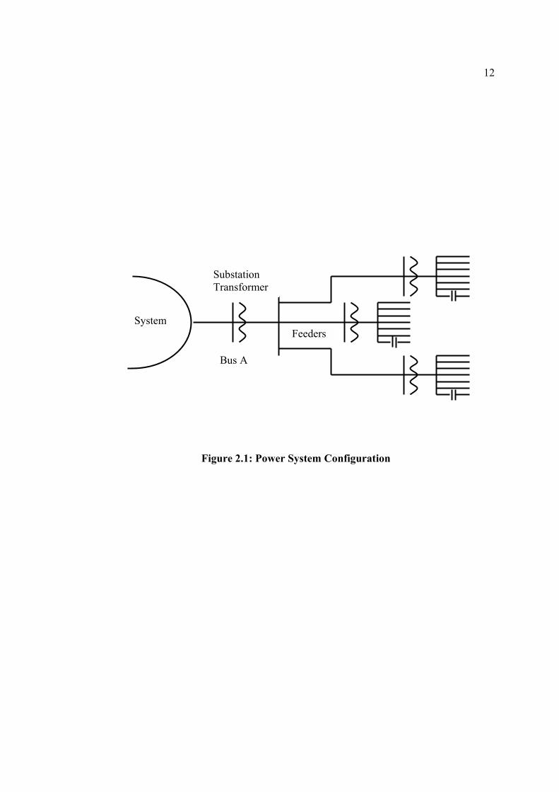
As illustrated in Figure 2.1, “load” in this context includes, not only the connected load
devices, but some or all of the following:
Substation Step-down transformer
Subtransmission feeders
Primary distribution feeders
Secondary distribution feeders
Shunt capacitors
Voltage regulators
Customer wiring, transformers and capacitors
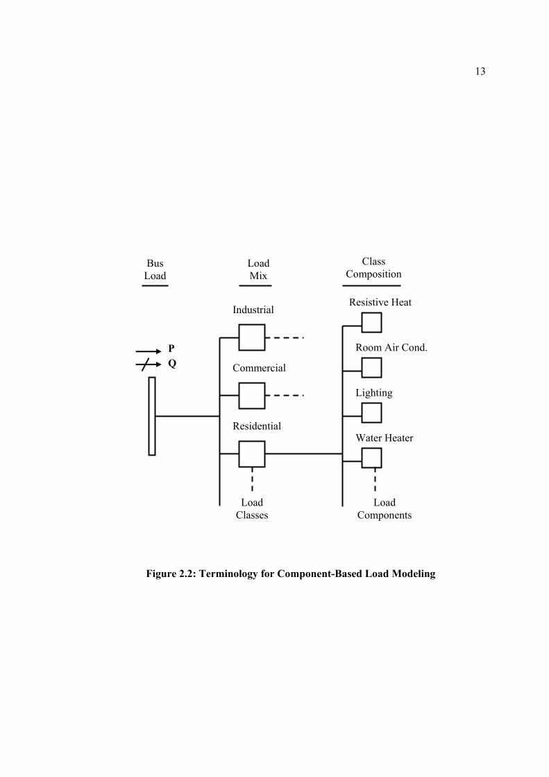
In describing the composition of load, the following terms, illustrated in Figure 2.2, are
recommended:
LOAD COMPONENT – a load component is the aggregate equivalent of all devices of a
specific or similar type, e.g., water heater, room air conditioner, fluorescent lighting.
LOAD CLASS – A load class is a category of load, such as, residential, commercial, or
industrial. For load modeling purposes, it is useful to group loads into several classes,
where each class has similar load composition and load characteristics.
12
Figure 2.1: Power System Configuration
SystemFeeders
Substation Transformer
Bus A
13
Figure 2.2: Terminology for Component-Based Load Modeling
Commercial
Residential
Bus Load
LoadMix
Class Composition
Industrial
P
Q
Resistive Heat
Room Air Cond.
Lighting
Water Heater
Load Classes
Load Components

14
RESIDENTIAL LOAD – It is defined as individual residences, individual flats,
individual apartments in multiple family residences, and religious institutions receiving
separately metered service.
COMMERCIAL LOAD – It is defined as institutions involved in trade.
INDUSTRIAL LOAD – It is defined as any enterprise engaged in extractive, fabricating,
or processing activities, which yield raw or unfinished materials, or which transform such
materials into another product.
LOAD COMPOSITION – It is the fractional composition of the load by load
components. This term may be applied to the bus load or to a specific load class.
LOAD CLASS MIX – It is the fractional composition of the bus load by load classes.
LOAD CHARACTERISTIC – A set of parameters, such as power factor, variation of P
and V, etc., that characterize the behavior of a specific load. This term may be applied to a
specific load device, a load component, a load class, or the total bus load.
The following terminology is commonly used in describing different types of load
models:

15
LOAD MODEL – A load model is a mathematical representation of the relationship
between a bus voltage (magnitude and frequency), weather factor and the power (active
and reactive) or current flowing into the bus load.
STATIC LOAD MODEL – A model that expresses the active and reactive powers at any
instant of time as functions of the voltage magnitude and frequency at the same time.
Static load models are used both for essentially static load components, e.g., resistive and
lighting load, and as an approximation for dynamic load components, e.g., motor-drive
loads.
DYNAMIC LOAD MODEL – A model that expresses the active and reactive powers at
any instant of time as functions of the voltage magnitude and frequency at past instants of
time and, usually, including the present instant. Difference or differential equations can be
used to represent such models.
CONSTANT IMPEDANCE LOAD MODEL – A static load model where the power
varies directly with the square of the voltage magnitude. It may also be called a constant
admittance load model.
CONSTANT CURRENT LOAD MODEL – A static load model where the power
varies directly with the voltage magnitude.
CONSTANT POWER LOAD MODEL – A static load model where the power does not
vary with changes in voltage magnitude. It may also be called constant MVA load model.

16
Because constant MVA devices, such as motors and electronic devices do not maintain
this characteristic below some voltage (typically 80 to 90%), many load models provide
for changing constant MVA (and other static models) to constant impedance or tripping
the load below a specified voltage. [1, 3, 7]
In the coming sections a brief overview of load model theory, load model derivation and
load model parameter estimation will be presented.
3.2 Load Model Theory
Two main approaches to load model development have been considered by the electric
utility industry:
“Measurement-based models” and “Component-based models.”
The measurement-based approach involves placing monitors at various load substations to
determine the sensitivity of load active and reactive power to voltage, frequency and
weather variations to be used directly or to identify parameters for more detailed load
models [1, 7].
The purpose of the component-based approach is to develop load models by aggregating
models of the individual components forming the load. Individual components
characteristics have been determined by theoretical and laboratory analysis and have been

17
extensively reported in literature. This approach is shown schematically in Figure 2.2 in
section 2 [4].
3.3 Load Model Derivation
The load at a bus in a power flow study can be represented as a function of voltage in a
number of ways.
• Polynomial Load Model
A static load model that represents the power relationship to voltage magnitude as a
polynomial equation, usually in the following form:
+
+
= 32
2
1 aVVa
VVaPP
ooo [3.1]
+
+
= 65
2
4 aVVa
VVaQQ
ooo [3.2]
The parameters of this model are the coefficients (a1 to a6) and the power factor of the
load. This model is sometimes referred to as the “ZIP” model, since it consists of the sum
of constant impedance (Z), constant current (I), and constant power (P) terms. If this, or
other, models are used for representing a specific load device, and Po and Qo should be the
power consumed at rated voltage Vo. However, when using these models for representing

18
a bus load, Vo, Po, and Qo are normally taken as the values at the initial system operating
condition for the study. [3]
• Exponential Load Model
A static load model that represents the power relationship to voltage as an exponential
equation, usually in the following form:
np
ooA V
VPP
=
[3.3]
np
ooA V
VQQ
=
[3.4]
Where
PA, QA = Actual real and reactive load powers
Po, Qo = Nominal real and reactive load powers
Vo = Nominal voltage at which Po, Qo are calculated
V = Actual voltage
np = Real power voltage exponent
nq = Reactive power voltage exponent
The parameters (np and nq) determine which load model is used to represent the load
power viz.

19
np = nq = 2
This is commonly called the constant impedance load model (Z) where the load power
varies directly with the square of the voltage magnitude. It may also be called a constant
admittance model. At below nominal voltages, this type of load will draw less current.
The opposite applies at above nominal voltages. Constant current loads will have a
tendency to decrease (or reduce) voltage oscillations on a system.
np = nq = 1
This is commonly called the constant current load model (I) where the load power varies
directly with the voltage magnitude. It has been accepted that, in the absence of data,
composite loads can be approximated using a constant current load model.
np = nq = 0
This is commonly called the constant power load model (P) where the load power does
not vary with changes in the voltage magnitude. It may also be called a constant MVA
model. This type of load draws higher current under low voltage conditions to maintain
constant power. It is thus very onerous on the system. [4]
• Frequency-Dependent Load Model
A static load model that includes frequency dependence. This is usually represented by
multiplying either a polynomial or exponential load model by a factor of the following
form:

20
( )[ ]of ffa −+1 [3.5]
where f is the frequency of the bus voltage, fo is the rated frequency, and af is the
frequency sensitivity parameter of the model. [3]
Examples of Load Models of Previous Forms
Example of ZIP Model
In reference [2], ZIP load models derived from measurements.
+
+
= P
oP
oPototal P
VVI
VVZPP ***
2
[3.6]
+
+
= q
oq
oqototal P
VVI
VVZQQ ***
2
[3.7]
where Z, I and P are constant impedance, constant current and constant power fractions
respectively.
The ZIP model is appropriate for both steady-state and dynamic studies for voltages above
the minimum voltage (Vmin).

21
Example of Exponential Load Model
In reference [13], the following load model is employed.
pnVKP *= [3.8]
qnno VKKQ *+= [3.9]
∆
∆
=
o
op
VV
PP
n [3.10]
∆
∆
=
o
oq
VV
n [3.11]
where
np = voltage slope of active power.
nq = voltage slope of reactive power.
Ko = initial power value.
Kn = voltage-dependent gain.

22
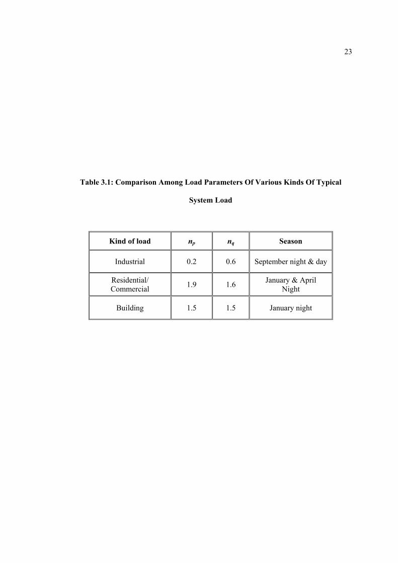
Table 3.1 shows the comparison of the load parameters among three types of system loads
already mentioned. When the parameters nq was calculated, the absolute of Ko was
assumed to be equal to the apparent power. For the industrial load, the value of parameter
np is approximately zero, indicating that this load is predominantly occupied by induction
motors. The parameter np of the residential/commercial load is close to 2.0. this is because
the load contains predominantly constant impedance load elements. The parameter np of
the building load is 1.5, showing that various kind of load element are included in this
load [10].
These values of parameters correspond to the features of the three types of load, which
were seen in the comparison of power responses.
From this result, it is obvious that the characteristics of the system load are closely
associated with its load composition. The values of parameters, therefore, vary according
to the variation in working rate of the load elements. For example, an increase in the
power consumed by air-conditioners may lower the load parameter of the total composite
load.
23
Table 3.1: Comparison Among Load Parameters Of Various Kinds Of Typical
System Load
Kind of load np nq Season
Industrial 0.2 0.6 September night & day
Residential/ Commercial 1.9 1.6 January & April
Night
Building 1.5 1.5 January night

24
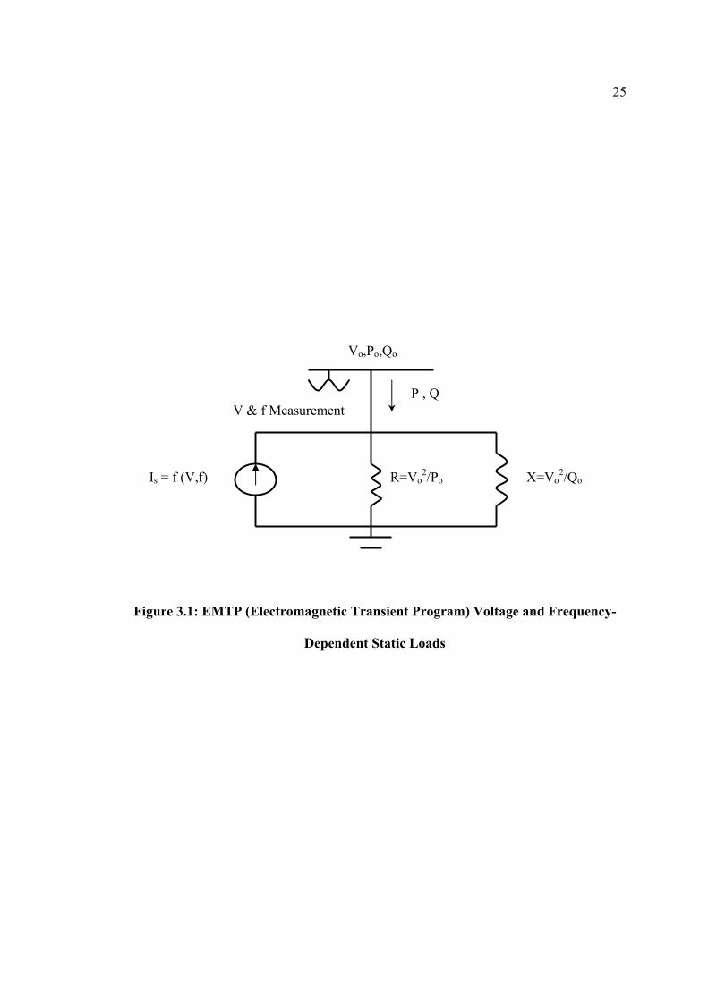
Example of Voltage and Frequency-Dependent Loads
Voltage and frequency-dependent loads such as televisions and fluorescent lighting are
simulated by passive elements and a current source (figure 3.1), which is adjusted to
satisfy the following formulas:
( )
−+
=
o
op
N
oo f
ffK
VVPP
p
1 [3.12]
( )
−+
=
o
oq
N
oo f
ffK
VVQQ
q
1 [3.13]
In reference [11], there is many load models summarized from many different cases in
previous work done in this field.
25
Figure 3.1: EMTP (Electromagnetic Transient Program) Voltage and Frequency-
Dependent Static Loads
Vo,Po,Qo
V & f Measurement
Is = f (V,f) R=Vo2/Po X=Vo
2/Qo
P , Q

26
3.4 Load Model Parameter Estimation
Parameter estimation techniques are used for evaluating the required model parameters.
Many iterative computational methods are considered in load model parameters
estimation:
(i). Newton Method
(ii). Modified Newton method
(iii). Broyden, Fletcher, Goldfarb and Shanno (BFGS) method
(iv). Modified BFGS method
The first method, or Newton method, is well known in the power systems engineering
area. The second method is a modification of the Newton method such that after each
iteration the updated values of the coefficients are discarded, and new values for the
coefficients are calculated using the current exponents so as to obtain a minimum sum of
the squares of the error (SSE). The third method is an extension to the Newton method
devised by Broyden, Fletcher, Goldfarb and Shanno and it is commonly referred to as the
BFGS method. The BFGS method is recommended in cases where the standard Newton
method fails to converge. This method employs a line search that steers the iterations in
the required direction and often converges even if the regular Newton method fails.
Fourth method is the same as third method (BFGS method) with similar modification as
in second method (Modified Newton method). [8]

27
Genetic algorithms (GA) methods also used in load modeling or parameter estimation.
GA is search algorithms for finding the optimum solutions of maximization problems. GA
simulates the natural selection mechanism of biological systems such as reproduction,
crossover and mutation. The main features of GA are a coding of the parameter set in the
problem, a multi-point search algorithm, no necessity of the information about the
derivative of objective function, and the probabilistic transition rules. These features
contribute to a genetic algorithm’s robustness and increase the likelihood of finding the
global optimal solution. [13]
Also, load parameters are derived from existing data using curve-fitting techniques for
both of static and dynamic components. Based on many graphs for developing models
describing load responses to weather variations is a load-weather correlation curves; i.e., a
plot of real and reactive powers as functions of weather. Least squared error curve fitting
is one of the methods used parameter estimation. [9]

28
Chapter 4
PROBLEM DEFINITION AND
OBJECTIVE In the coming sections and overview of problem definition and objective will be
presented.
4.1 Problem Definition
Of all the other factors that give rise to system peak demand, weather is the main factor,
which dictates the peak load significantly. If other contributing factors to peak load are
neglected the system demand will move in harmony with ambient temperatures and
humidity, and the peak demand will occur during the period of high temperatures and/or
high humidity.
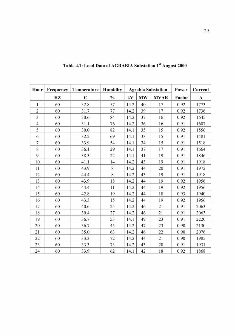
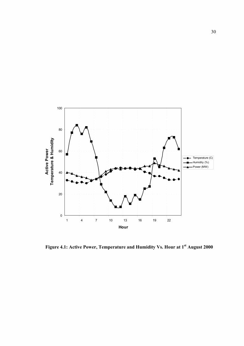
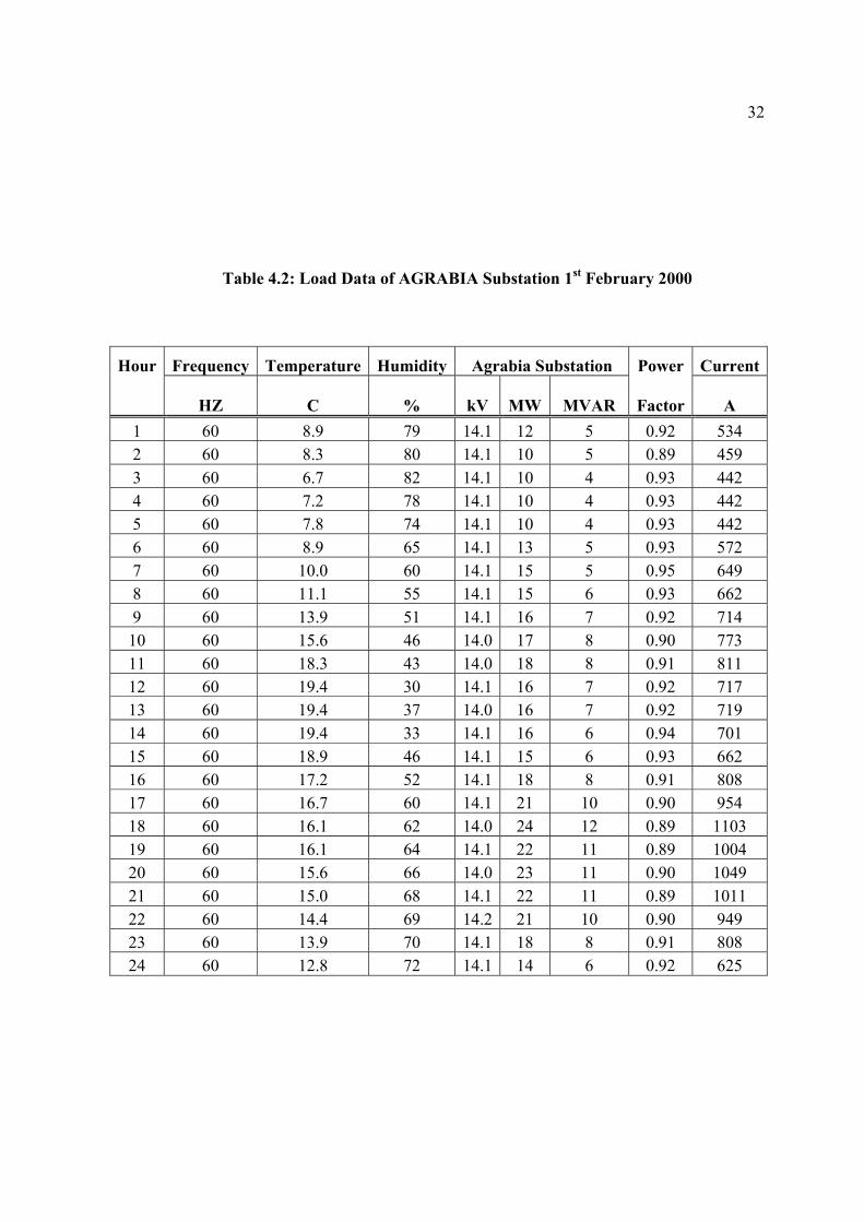
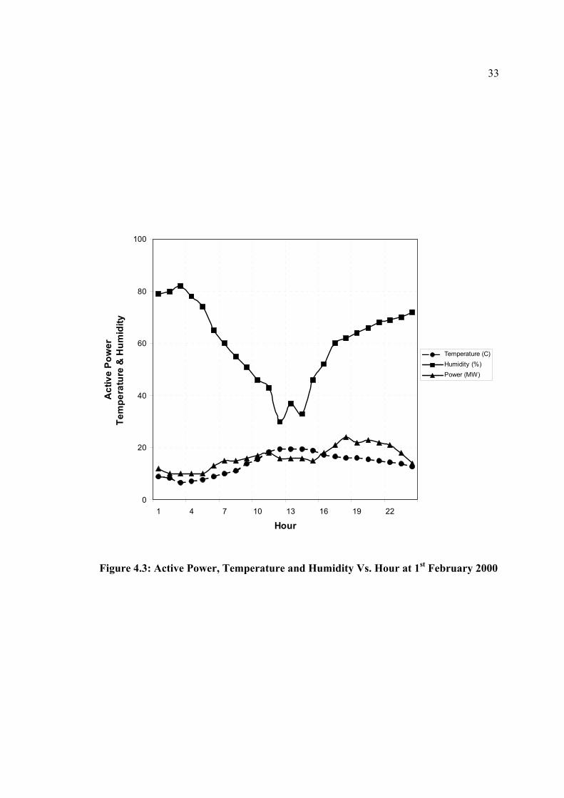
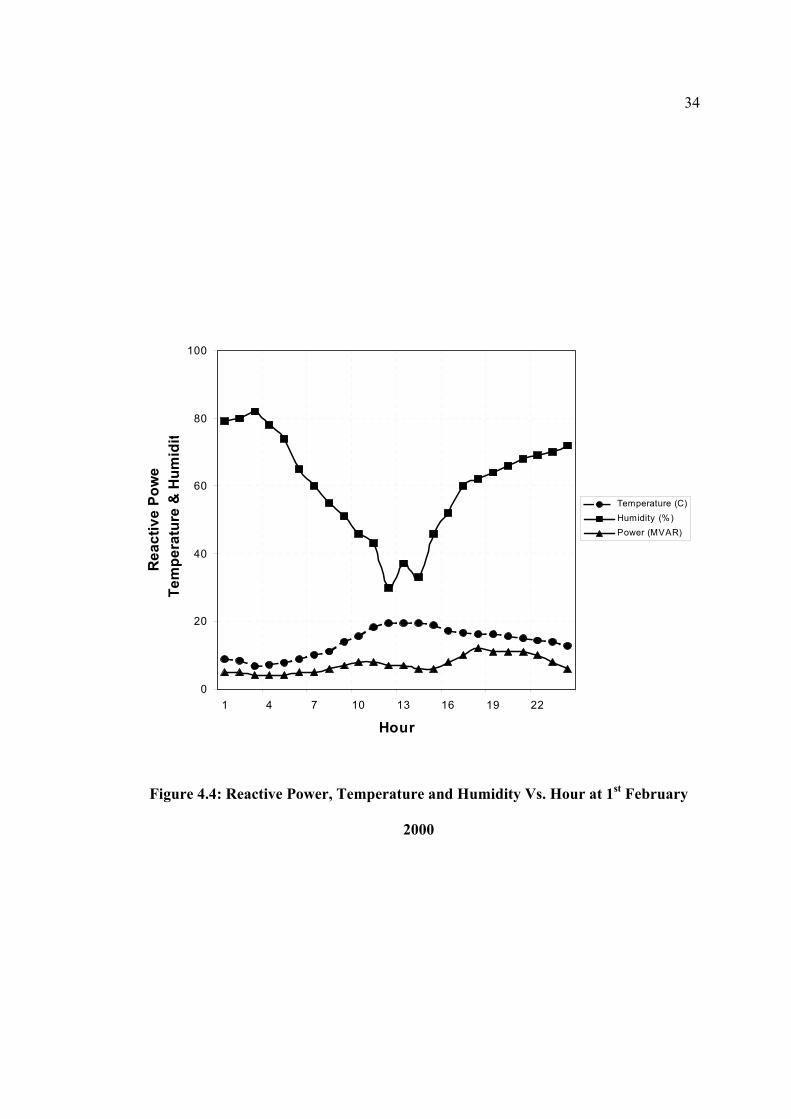
Tables 4.1 and 4.2 show sample of load research data brought from utility. Figures 4.1
and 4.3 show the plots of active power, temperature and humidity versus time (hour).
Where as figures 4.2 and 4.4 show the plots of reactive power, temperature and humidity
versus time (hour)
28
29
Table 4.1: Load Data of AGRABIA Substation 1st August 2000
Hour Frequency Temperature Humidity Agrabia Substation Power Current
HZ C % kV MW MVAR Factor A 1 60 32.8 57 14.2 40 17 0.92 1773 2 60 31.7 77 14.2 39 17 0.92 1736 3 60 30.6 84 14.2 37 16 0.92 1645 4 60 31.1 76 14.2 36 16 0.91 1607 5 60 30.0 82 14.1 35 15 0.92 1556 6 60 32.2 69 14.1 33 15 0.91 1481 7 60 33.9 54 14.1 34 15 0.91 1518 8 60 36.1 29 14.1 37 17 0.91 1664 9 60 38.3 22 14.1 41 19 0.91 1846
10 60 41.1 14 14.2 43 19 0.91 1918 11 60 43.9 8 14.2 44 20 0.91 1972 12 60 44.4 8 14.2 43 19 0.91 1918 13 60 43.9 18 14.2 44 19 0.92 1956 14 60 44.4 11 14.2 44 19 0.92 1956 15 60 42.8 19 14.2 44 18 0.93 1940 16 60 43.3 15 14.2 44 19 0.92 1956 17 60 40.6 25 14.2 46 21 0.91 2063 18 60 39.4 27 14.2 46 21 0.91 2063 19 60 36.7 53 14.1 49 23 0.91 2220 20 60 36.7 45 14.2 47 23 0.90 2130 21 60 35.0 63 14.2 46 22 0.90 2076 22 60 33.3 72 14.2 44 21 0.90 1985 23 60 33.3 73 14.2 43 20 0.91 1931 24 60 33.9 62 14.1 42 18 0.92 1868
30
Figure 4.1: Active Power, Temperature and Humidity Vs. Hour at 1st August 2000
0
20
40
60
80
100
1 4 7 10 13 16 19 22
Hour
Act
ive
Pow
er T
empe
ratu
re &
Hum
idity
Temperature (C)Humidity (%)Power (MW)

31
Figure 4.2: Reactive Power, Temperature and Humidity Vs. Hour at 1st August 2000
0
20
40
60
80
100
1 4 7 10 13 16 19 22
Hour
Rea
ctiv
e Po
wer
Tem
pera
ture
& H
umid
ity
Temeprature (C)Humidity (%)Power (MVAR)
32
Table 4.2: Load Data of AGRABIA Substation 1st February 2000
Hour Frequency Temperature Humidity Agrabia Substation Power Current
HZ C % kV MW MVAR
Factor A 1 60 8.9 79 14.1 12 5 0.92 534 2 60 8.3 80 14.1 10 5 0.89 459 3 60 6.7 82 14.1 10 4 0.93 442 4 60 7.2 78 14.1 10 4 0.93 442 5 60 7.8 74 14.1 10 4 0.93 442 6 60 8.9 65 14.1 13 5 0.93 572 7 60 10.0 60 14.1 15 5 0.95 649 8 60 11.1 55 14.1 15 6 0.93 662 9 60 13.9 51 14.1 16 7 0.92 714
10 60 15.6 46 14.0 17 8 0.90 773 11 60 18.3 43 14.0 18 8 0.91 811 12 60 19.4 30 14.1 16 7 0.92 717 13 60 19.4 37 14.0 16 7 0.92 719 14 60 19.4 33 14.1 16 6 0.94 701 15 60 18.9 46 14.1 15 6 0.93 662 16 60 17.2 52 14.1 18 8 0.91 808 17 60 16.7 60 14.1 21 10 0.90 954 18 60 16.1 62 14.0 24 12 0.89 1103 19 60 16.1 64 14.1 22 11 0.89 1004 20 60 15.6 66 14.0 23 11 0.90 1049 21 60 15.0 68 14.1 22 11 0.89 1011 22 60 14.4 69 14.2 21 10 0.90 949 23 60 13.9 70 14.1 18 8 0.91 808 24 60 12.8 72 14.1 14 6 0.92 625
33
Figure 4.3: Active Power, Temperature and Humidity Vs. Hour at 1st February 2000
0
20
40
60
80
100
1 4 7 10 13 16 19 22
Hour
Act
ive
Pow
erTe
mpe
ratu
re &
Hum
idity
Temperature (C)Humidity (%)Power (MW)
34
Figure 4.4: Reactive Power, Temperature and Humidity Vs. Hour at 1st February
2000
0
20
40
60
80
100
1 4 7 10 13 16 19 22
Hour
Rea
ctiv
e Po
we
Tem
pera
ture
& H
umid
i t
Temperature (C)Humidity (%)Power (MVAR)

35
As can be seen from figure 4.1 (summer example), the power consumption is following
the temperature rises. Figure 4.1 also shows that temperature effect is more dominant than
the relative humidity effect.
As shown in figure 4.3 (winter example) the power consumption is reduced during the
winter almost by the half. Moreover, it can be seen that the humidity effect is not
significant.
Figures 4.2 and 4.4, which are for the reactive power consumption, confirm that the
reactive power consumption also effected by weather condition. The reactive power
consumed in summer is almost double the one consumed in winter. This high increase is
due to the air conditioning load.
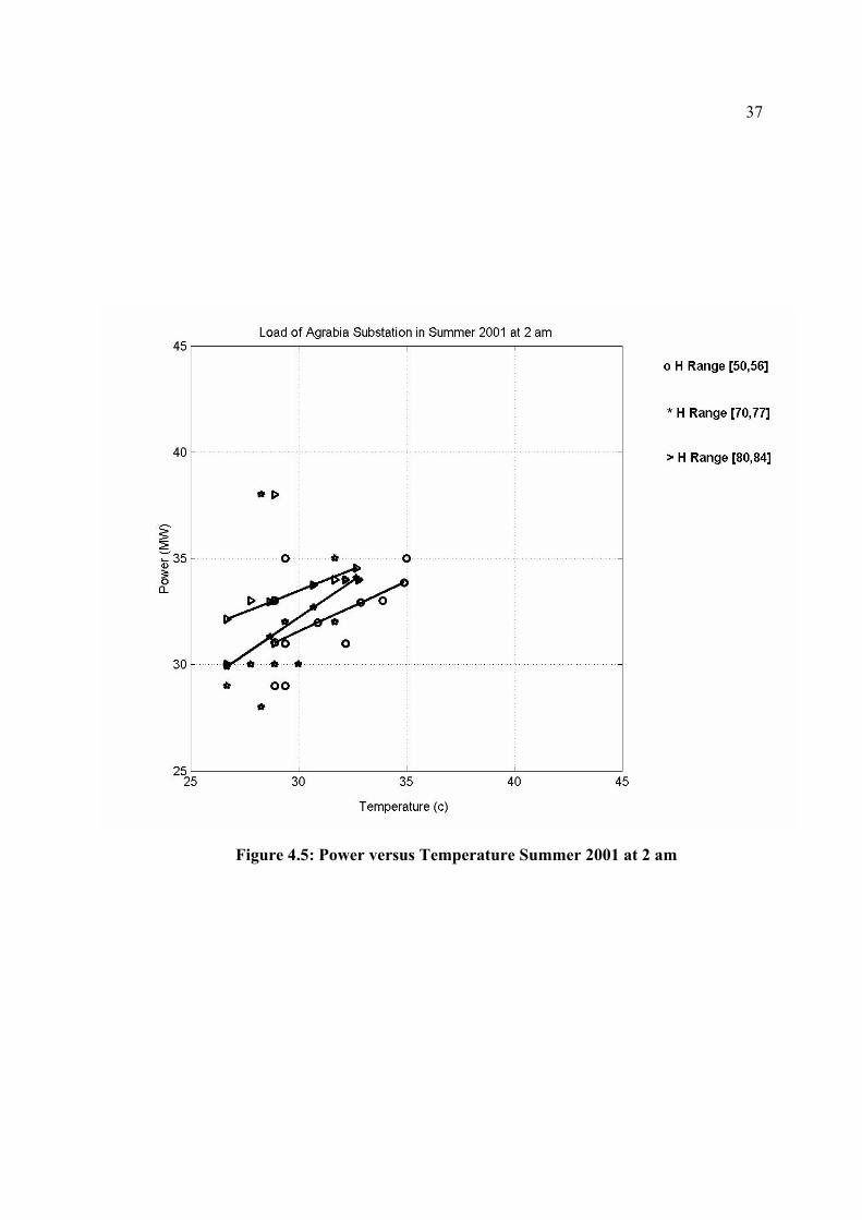
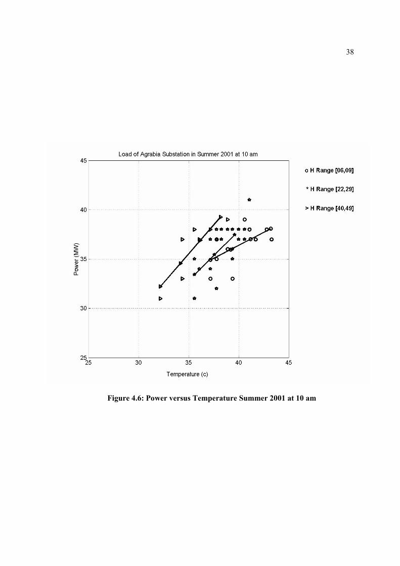
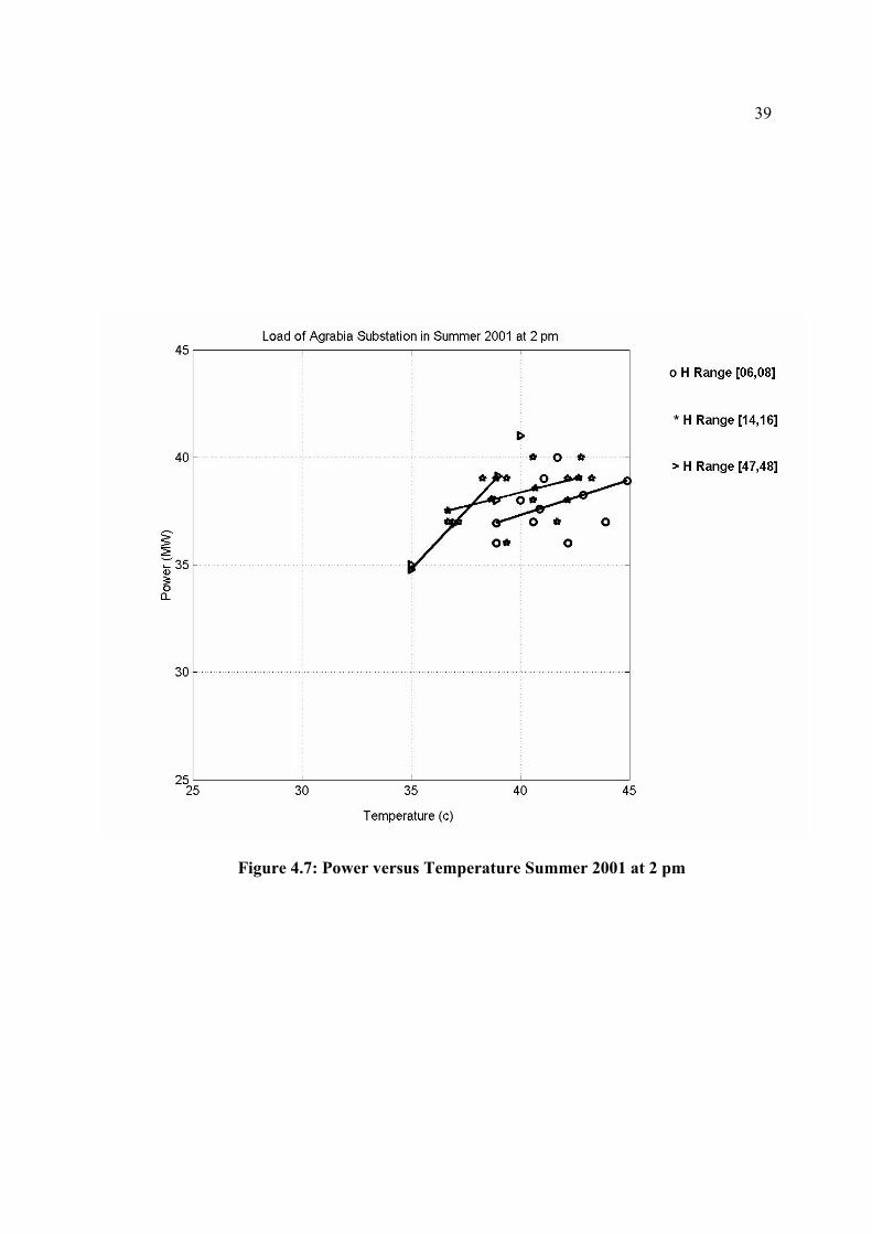
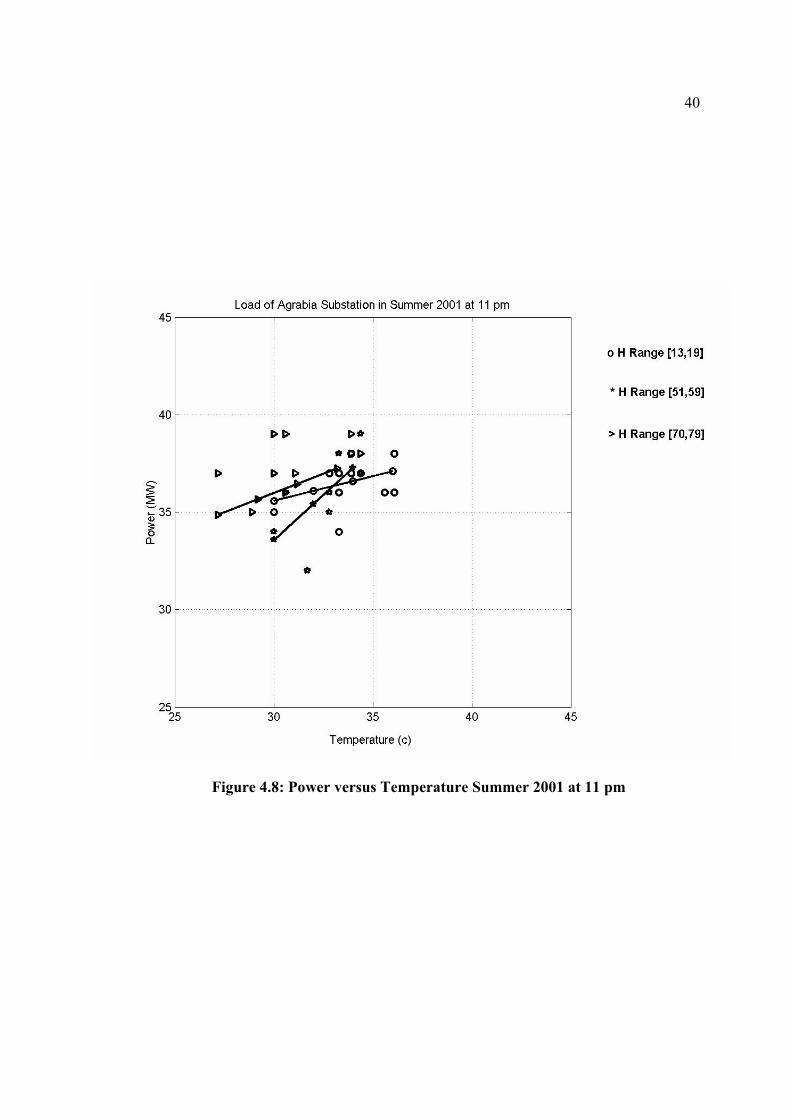
Figures 4.5 to 4.8 show the plots of active power versus temperature where the change in
relative humidity is limited with small interval for summer period. These figures illustrate
four different cases of environmental impact on residential load consumption.
First case is shown in figure 4.5 where the temperature is low and the relative humidity is
high. So, the power consumption is low. Figure 4.6 shows the second case where the
temperature is moderate and the relative humidity is low. In this case the power demand
start to increase due to the increase in the temperature. The maximum temperature is
occurring in the third case where the relative humidity is low. It can be seen from figure
4.7 that the power consumption is reaching their maximum value compared to the other

36
cases. In the last case, average power consumption is shown in figure 4.8 due to moderate
temperature and varying relative humidity.
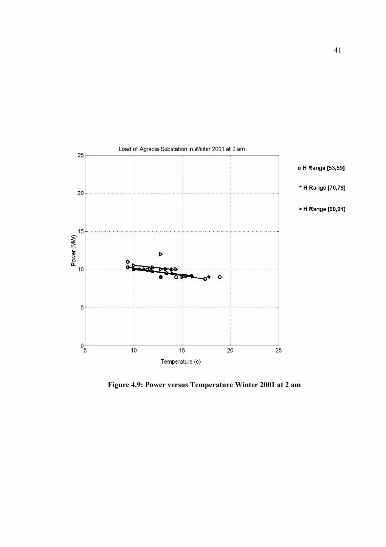
Figures 4.9 and 4.10 show the plots of active power versus temperature where the change
in relative humidity is limited with small interval for winter period. These figures
represent two different cases.
In the first case, the temperature is low and the relative humidity is high. However, in the
second case both the temperature and the relative humidity are low. In both cases the
power consumptions can be assumed constant.
On an hourly basis, the large dependence of the load demand on temperature is quit
apparent as shown in the previous figures. However, preliminary analyses indicate that the
relative humidity is not a major determinant of the maximum demand requirements of
residential customers. Also, this is the conclusion approached by utility engineers [5, 6].
Hourly load profiles also show that maximum demand increases in summer because of the
dominant air conditioning load.
In summary, the summer figures reveal that the residential loads are relatively more
sensitive to the change in temperature than the change in the relative humidity. However,
the temperature variations during the winter have minor effect on the power requirements.
This is because the power requirement for heating purposes during the winter season is
not significant.
37
Figure 4.5: Power versus Temperature Summer 2001 at 2 am
38
Figure 4.6: Power versus Temperature Summer 2001 at 10 am
39
Figure 4.7: Power versus Temperature Summer 2001 at 2 pm
40
Figure 4.8: Power versus Temperature Summer 2001 at 11 pm
41
Figure 4.9: Power versus Temperature Winter 2001 at 2 am
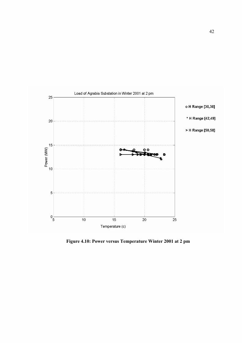
42
Figure 4.10: Power versus Temperature Winter 2001 at 2 pm

43
4.2 Objective
In the previous section a detailed discussion about the power demand relation with
temperature and relative humidity was presented. This relation cannot be shown by a
simpler straight-line model, since the plots show a non-linear relation between power
demand, temperature and relative humidity.
The aim of this work is to find forms of power system static load models representing the
variation of active and reactive power with the temperature and relative humidity, in term
of the associated model parameter estimation.
The load model selected for parameter estimation in this research is the polynomial load
model (Equation 3.1 and 3.2) where the active and reactive power is function of
temperature and relative humidity. Also, equations 4.1 and 4.2 show a brief formulation of
this relation.
( )HTFP ,= [4.1]
( )HTFQ ,= [4.2]
In the next chapter, the active and reactive power models results and discussion will be
presented in more details.

44
Chapter 5
LOAD MODEL RESULTS AND
DISCUSSION
This chapter gives a detail discussion about the process, procedure, formulation and
testing of load modeling derivation.
5.1 Parameter Estimation Method
One of the most important problems in technical computing is the solution of
simultaneous linear equations [14]. In matrix notation, this problem can be stated as
Ax=B. Similar considerations apply to sets of nonlinear equations with more than one
unknown. MATLAB solves such equations without computing the inverse of the matrix.
Identification of the coefficient of the function often leads to the formulation of an over-
determined system of simultaneous nonlinear equations for experimental data and field
measurement data.
44

45
Over-determined systems of simultaneous nonlinear equations Ax=B obtained with A as
non-square matrix, x is the coefficients vector and B is the field data points. Therefore
solves for unknown coefficients by performing a least squares solution is achieved using a
QR factorization technique which allows the minimization of ||Ax-B||. [15]
Multiple regression solves for unknown coefficients by performing a least squares fit.
Construct and solve the set of simultaneous equations by forming the regression matrix
and solving for the coefficients using the backslash operator. The coming section
illustrates the multiple regression method with an example.
5.2 EPRI Load Model Example
The following example is taken from EPRI report [7]. EPRI derived the model for this
example using their program LOADSYN (Load Model Synthesis program package),
which was developed to convert load composition and load characteristic data into
parameters required for the power flow and transient stability programs.
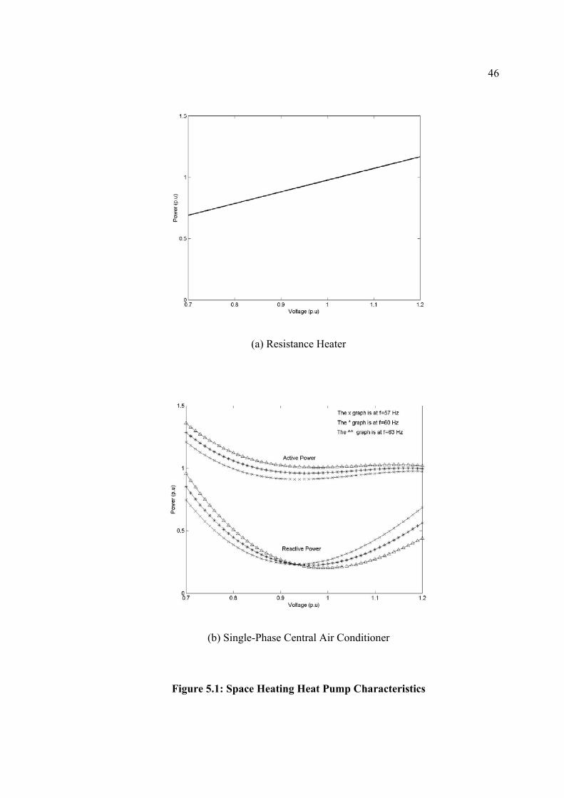
This example is for a heat pump, which consists of a resistance heater and a single-phase
central air conditioner. These devices have characteristics as shown in figure 5.1, which
were taken from EPRI report. Table 5.1 shows the data for voltage (V), frequency (f),
active power (P), reactive power (Q) and power (KVA) of this heat pump.
An assumed model structure is given in equations 5.1 and 5.2, where VR, fR are equal to
one.
46
(a) Resistance Heater
(b) Single-Phase Central Air Conditioner
Figure 5.1: Space Heating Heat Pump Characteristics

47
( ) ( ) ( ) ( ) ( )( )RRRRRR ffVVcffbVVaVVaVVaaP −−+−+−+−+−+= 113
32
210 [5.1]
( ) ( ) ( ) ( ) ( )( )RRRRRR ffVVcffbVVaVVaVVaaQ −−+−+−+−+−+= 113
32
210 [5.2]
This model structure is used because it is the same model structure used by EPRI. Also, to
compare the model will be derived with the model derived by EPRI.
As explained in section 5.1 solves for unknown coefficients a0, a1, a2, a3, b1, and c1 by
performing a least squares technique (QR factorization technique). Construct and solve
the set of simultaneous equations by forming the matrix X and solving for the coefficients.
V = V – VR
F = f - fR
X = [ones(size(V)) V V2 V3 F V*F]
Table 5.2 shows the complete data of matrix X. Therefore, the complete models are:
FVFVVVP 0886.28690.07778.85994.11942.09640.0 32 −+−++= [5.3]
FVFVVVQ 1200.96240.03111.67695.65380.02340.0 32 −−−++= [5.4]
The model, thus obtained, is same as the model obtained by EPRI. So, the load model
parameters estimated without any error by using different approach than the EPRI used.
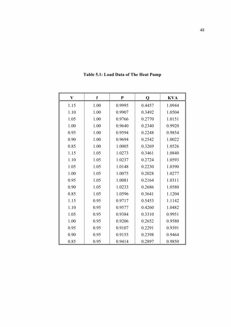
48
Table 5.1: Load Data of The Heat Pump
V f P Q KVA
1.15 1.00 0.9995 0.4457 1.0944 1.10 1.00 0.9907 0.3492 1.0504 1.05 1.00 0.9766 0.2770 1.0151 1.00 1.00 0.9640 0.2340 0.9920 0.95 1.00 0.9594 0.2248 0.9854 0.90 1.00 0.9694 0.2542 1.0022 0.85 1.00 1.0005 0.3269 1.0526 1.15 1.05 1.0273 0.3461 1.0840 1.10 1.05 1.0237 0.2724 1.0593 1.05 1.05 1.0148 0.2230 1.0390 1.00 1.05 1.0075 0.2028 1.0277 0.95 1.05 1.0081 0.2164 1.0311 0.90 1.05 1.0233 0.2686 1.0580 0.85 1.05 1.0596 0.3641 1.1204 1.15 0.95 0.9717 0.5453 1.1142 1.10 0.95 0.9577 0.4260 1.0482 1.05 0.95 0.9384 0.3310 0.9951 1.00 0.95 0.9206 0.2652 0.9580 0.95 0.95 0.9107 0.2291 0.9391 0.90 0.95 0.9155 0.2398 0.9464 0.85 0.95 0.9414 0.2897 0.9850
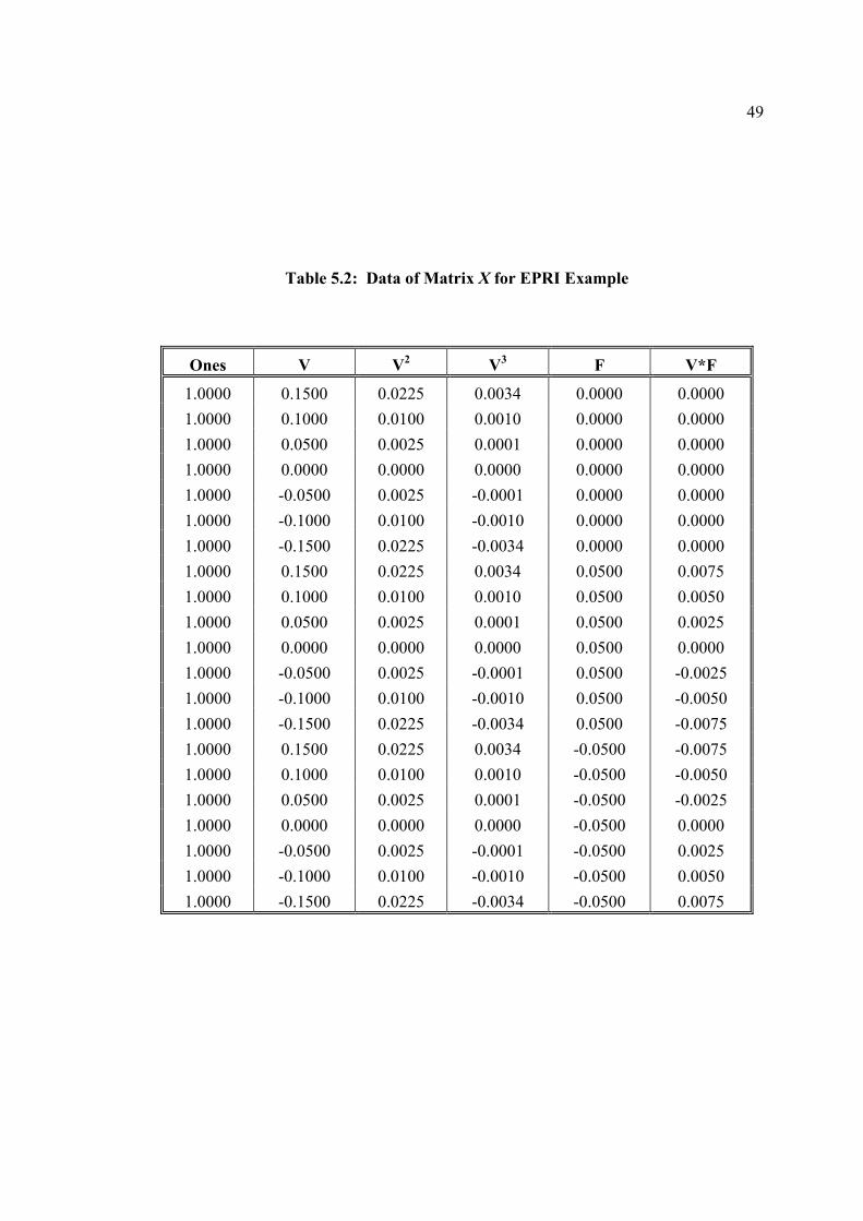
49
Table 5.2: Data of Matrix X for EPRI Example
Ones V V2 V3 F V*F
1.0000 0.1500 0.0225 0.0034 0.0000 0.0000 1.0000 0.1000 0.0100 0.0010 0.0000 0.0000 1.0000 0.0500 0.0025 0.0001 0.0000 0.0000 1.0000 0.0000 0.0000 0.0000 0.0000 0.0000 1.0000 -0.0500 0.0025 -0.0001 0.0000 0.0000 1.0000 -0.1000 0.0100 -0.0010 0.0000 0.0000 1.0000 -0.1500 0.0225 -0.0034 0.0000 0.0000 1.0000 0.1500 0.0225 0.0034 0.0500 0.0075 1.0000 0.1000 0.0100 0.0010 0.0500 0.0050 1.0000 0.0500 0.0025 0.0001 0.0500 0.0025 1.0000 0.0000 0.0000 0.0000 0.0500 0.0000 1.0000 -0.0500 0.0025 -0.0001 0.0500 -0.0025 1.0000 -0.1000 0.0100 -0.0010 0.0500 -0.0050 1.0000 -0.1500 0.0225 -0.0034 0.0500 -0.0075 1.0000 0.1500 0.0225 0.0034 -0.0500 -0.0075 1.0000 0.1000 0.0100 0.0010 -0.0500 -0.0050 1.0000 0.0500 0.0025 0.0001 -0.0500 -0.0025 1.0000 0.0000 0.0000 0.0000 -0.0500 0.0000 1.0000 -0.0500 0.0025 -0.0001 -0.0500 0.0025 1.0000 -0.1000 0.0100 -0.0010 -0.0500 0.0050 1.0000 -0.1500 0.0225 -0.0034 -0.0500 0.0075

50
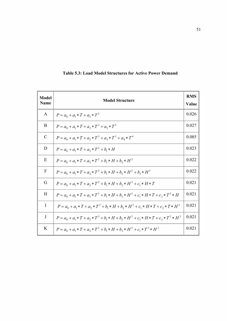
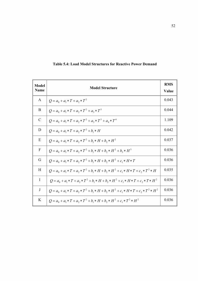
5.3 Load Modeling Structure Selection
As mentioned in chapter four the power demand is more affected by the temperature
change. Also, it was mentioned that the relation between power demand, temperature and
relative humidity couldn’t be shown by a simpler straight-line model, since the plots show
a non-linear relations. So, selecting appropriate load model structure for active and
reactive power demand can be started from these points.
Tables 5.3 and 5.4 show different types of active and reactive power demand load model
structures. Also, appendix-A gives more detailed information about these models.
Models G in both tables 5.3 and 5.4 were selected based on the following:
• Model G gives the minimum RMS (Root Mean Square) value.
• Adding higher order terms did not reduce the RMS value.
• From a practical implementation point of view, it is clearly preferable to adopt
models of low order to reduce the computational burden in the parameter
estimation task.
51
Table 5.3: Load Model Structures for Active Power Demand
Model Name Model Structure
RMS
Value
A 2210 TaTaaP ∗+∗+= 0.026
B 33
2210 TaTaTaaP ∗+∗+∗+= 0.027
C 44
33
2210 TaTaTaTaaP ∗+∗+∗+∗+= 0.085
D HbTaTaaP ∗+∗+∗+= 12
210 0.023
E 221
2210 HbHbTaTaaP ∗+∗+∗+∗+= 0.022
F 33
221
2210 HbHbHbTaTaaP ∗+∗+∗+∗+∗+= 0.022
G THcHbHbTaTaaP ∗∗+∗+∗+∗+∗+= 12
212
210 0.021
H HTcTHcHbHbTaTaaP ∗∗+∗∗+∗+∗+∗+∗+= 221
221
2210 0.021
I 221
221
2210 HTcTHcHbHbTaTaaP ∗∗+∗∗+∗+∗+∗+∗+= 0.021
J 2221
221
2210 HTcTHcHbHbTaTaaP ∗∗+∗∗+∗+∗+∗+∗+= 0.021
K 221
221
2210 HTcHbHbTaTaaP ∗∗+∗+∗+∗+∗+= 0.021
52
Table 5.4: Load Model Structures for Reactive Power Demand
Model Name Model Structure
RMS
Value
A 2210 TaTaaQ ∗+∗+= 0.043
B 33
2210 TaTaTaaQ ∗+∗+∗+= 0.044
C 44
33
2210 TaTaTaTaaQ ∗+∗+∗+∗+= 1.109
D HbTaTaaQ ∗+∗+∗+= 12
210 0.042
E 221
2210 HbHbTaTaaQ ∗+∗+∗+∗+= 0.037
F 33
221
2210 HbHbHbTaTaaQ ∗+∗+∗+∗+∗+= 0.036
G THcHbHbTaTaaQ ∗∗+∗+∗+∗+∗+= 12
212
210 0.036
H HTcTHcHbHbTaTaaQ ∗∗+∗∗+∗+∗+∗+∗+= 221
221
2210 0.035
I 221
221
2210 HTcTHcHbHbTaTaaQ ∗∗+∗∗+∗+∗+∗+∗+= 0.036
J 2221
221
2210 HTcTHcHbHbTaTaaQ ∗∗+∗∗+∗+∗+∗+∗+= 0.036
K 221
221
2210 HTcHbHbTaTaaQ ∗∗+∗+∗+∗+∗+= 0.036

53
5.4 Data For Load Modeling
One of the major important parts of this research is the data collection and manipulation.
This section discusses the data for load models, including both measurement-based and
component-based methods of obtaining data. Selected data is also discussed.
5.4.1 Basic Approaches to Obtain Data
As discussed briefly in chapter three, there are two basic approaches to obtain data for
load modeling measurement-based data and component-based data. The measurement-
based approach is to directly measure the voltage, frequency and weather conditions
sensitivity of active and reactive power at represented substations and feeders. The
component-based approach is to build up a composite load model from knowledge of the
mix of load classes and served by a substation, the composition of each class and typical
characteristics of each load component. [3]
• Measurement-Based Approach
Data for load modeling can be obtained by installing measurement and data acquisition
devices at points where bus load are to be represented. These devices must measure
voltage, frequency, and weather and the corresponding variation in active and reactive
power demand.
Several utilities have been developing systems to gather such data. Electricity utility in
eastern branch in Saudi Arabia uses a computerized database containing hourly data about
system generation, loads and weather [5].

54
Measurement-based techniques have the obvious advantage of obtaining data directly
from the actual system. However, there are several disadvantages, including:
Application of data gathered for load models at one substation may not only be
possible for other substations if the loads are very similar.
Determination of characteristics over a wide range of voltage and frequency may
be impractical.
Accounting for variation of load characteristics due to daily, seasonal, weather,
and end-use changes requires on-going measurements under these varying
conditions.
• Component-Based Approach
The purpose of the component-based approach is to develop load models by aggregating
models of individual components forming the load. Component characteristics, e.g., for
air conditioners, fluorescent lights, etc., can be determined by theoretical analysis and
laboratory measurements and, once determined, used by all utilities. Much of this data has
been determined and documented by EPRI project [7], although it needs to be updated for
new and redesigned load devices.
The composition-based approach to load modeling has the advantage of not requiring
field measurements and of being adaptable to different systems and conditions. Its main
disadvantage is in requiring the gathering of load class mix, and perhaps load composition
data, which are not normally used by power system analysis.

55
5.4.2 Data Selected
The residential load models reported in this research are based on available field data
which consists of five years, each of which has data points listing the temperature,
humidity, active power and reactive power versus time, for the load on a residential
substation in the Saudi Electricity Company in Eastern Region Branch (SEC-ERB).
The data is available in computerized files containing hourly data about generation,
voltage, frequency, load and weather.
For this research, the hourly demand data for the years 1998, 1999, 2000 and 2001 were
used for formulated residential load models. However, the year 2002 hourly demand data
was used for testing and validation of the formulated residential load models. The
literature [12] reveals that for such kinds of seasonal study of time series, historical data
for 5-6 years is sufficient.
As mentioned in chapter four the effect of weather in residential load is in summer period
where the temperature and relative humidity reach their maximum values. June, July,
August and September are the summer months where the variation in temperature and
relative humidity effect the power demand consumption.
In order to represent the effect of the weather condition on the residential load and
excluding any other load contributing variables, only the weekdays (Saturday, Sunday,
Monday, Tuesday and Wednesday) were included. Also, depending on the characteristics

56
and contribution of the non-temperature dependent load, hours 2 am and 2 pm were
selected. Appendix B gives a detail description of the original raw data and the selected
Agrabia substation data used to derive the residential load models.
These data has been selected to reflect the impact of temperature and relative humidity
and exclude the impact of the load variation.
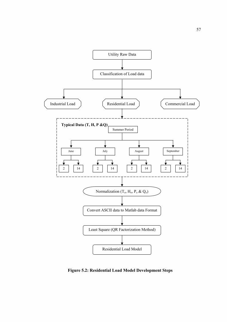
5.5 Load Model Development Steps
The flow chart of the steps developed to formulate the residential load models based on
the environmental factor is shown in figure 5.2.
Initially the raw data collected from utility will be classified based on the type of the load
(industrial, residential or commercial). Then a typical data will be selected.
The typical data will be selected for the summer period including the hot and the humid
months of the year (June, July, August and September) and the hours (2 am and 2 pm)
where the temperature and humidity are varying.
The data is normalized with respect to nominal values Po, Ho, To and Qo. Then the data
will be converted from ASCII format to MATLAB data file format. Finally, the
residential load models will be derived by applying the QR factorization method in the
MATLAB program.
57
Figure 5.2: Residential Load Model Development Steps
Utility Raw Data
Classification of Load data
Industrial Load Residential Load Commercial Load
Summer Period
June
2 14
July August September
Typical Data (T, H, P &Q)
Normalization (To, Ho, Po & Qo)
Residential Load Model
Convert ASCII data to Matlab data Format
Least Square (QR Factorization Method)
2 14 2 14 2 14
58
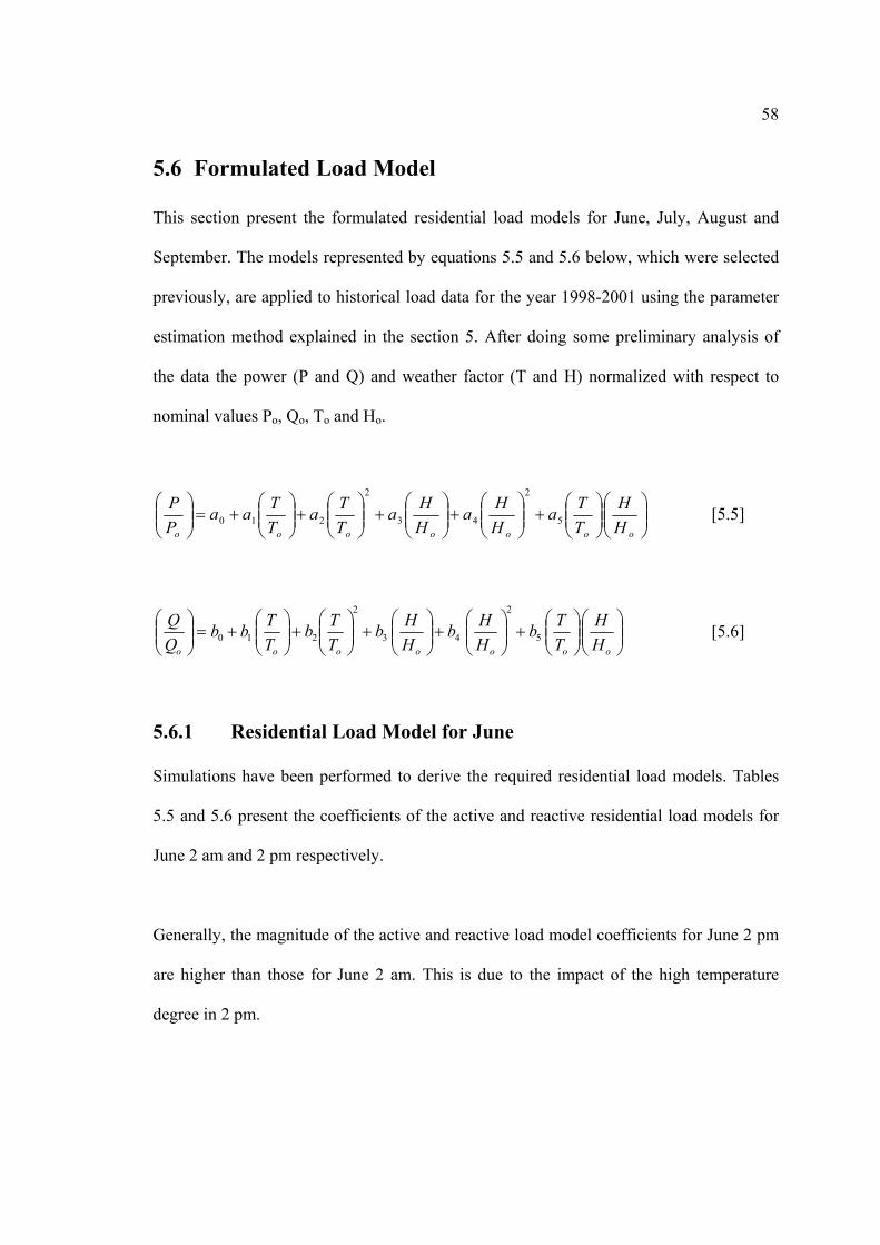
5.6 Formulated Load Model
This section present the formulated residential load models for June, July, August and
September. The models represented by equations 5.5 and 5.6 below, which were selected
previously, are applied to historical load data for the year 1998-2001 using the parameter
estimation method explained in the section 5. After doing some preliminary analysis of
the data the power (P and Q) and weather factor (T and H) normalized with respect to
nominal values Po, Qo, To and Ho.
+
+
+
+
+=
ooooooo HH
TTa
HHa
HHa
TTa
TTaa
PP
5
2
43
2
210 [5.5]
+
+
+
+
+=
ooooooo HH
TTb
HHb
HHb
TTb
TTbb
5
2
43
2
210 [5.6]
5.6.1 Residential Load Model for June
Simulations have been performed to derive the required residential load models. Tables
5.5 and 5.6 present the coefficients of the active and reactive residential load models for
June 2 am and 2 pm respectively.
Generally, the magnitude of the active and reactive load model coefficients for June 2 pm
are higher than those for June 2 am. This is due to the impact of the high temperature
degree in 2 pm.
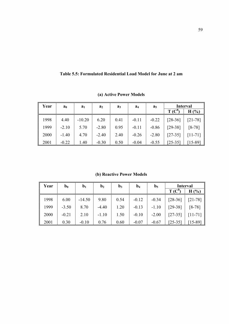
59
Table 5.5: Formulated Residential Load Model for June at 2 am
(a) Active Power Models
Year a0 a1 a2 a3 a4 a5 Interval T (C0) H (%)
1998 4.40 -10.20 6.20 0.41 -0.11 -0.22 [28-36] [21-78]
1999 -2.10 5.70 -2.80 0.95 -0.11 -0.86 [29-38] [8-78]
2000 -1.40 4.70 -2.40 2.40 -0.26 -2.80 [27-35] [11-71]
2001 -0.22 1.40 -0.30 0.50 -0.04 -0.55 [25-35] [15-89]
(b) Reactive Power Models
Year b0 b1 b2 b3 b4 b5 Interval T (C0) H (%)
1998 6.00 -14.50 9.80 0.54 -0.12 -0.34 [28-36] [21-78]
1999 -3.50 8.70 -4.40 1.20 -0.13 -1.10 [29-38] [8-78]
2000 -0.21 2.10 -1.10 1.50 -0.10 -2.00 [27-35] [11-71]
2001 0.30 -0.10 0.76 0.60 -0.07 -0.67 [25-35] [15-89]
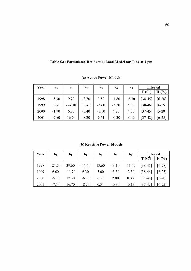
60
Table 5.6: Formulated Residential Load Model for June at 2 pm
(a) Active Power Models
Year a0 a1 a2 a3 a4 a5 Interval T (C0) H (%)
1998 -5.30 9.70 -3.70 7.50 -1.80 -6.30 [38-45] [6-28]
1999 13.70 -24.30 11.40 -3.60 -3.20 5.30 [38-46] [6-25]
2000 -1.70 6.30 -3.40 -6.10 4.20 4.00 [37-45] [5-20]
2001 -7.60 16.70 -8.20 0.51 -0.30 -0.13 [37-42] [6-25]
(b) Reactive Power Models
Year b0 b1 b2 b3 b4 b5 Interval T (C0) H (%)
1998 -21.70 39.60 -17.40 13.60 -3.10 -11.40 [38-45] [6-28]
1999 6.00 -11.70 6.30 5.60 -5.50 -2.50 [38-46] [6-25]
2000 -5.30 12.30 -6.00 -1.70 2.80 0.33 [37-45] [5-20]
2001 -7.70 16.70 -8.20 0.51 -0.30 -0.13 [37-42] [6-25]

61
However, the effect of the humidity is different. When the magnitude of the humidity
coefficients are high (2 pm models), the range of the humidity values are low (5 to 30
percent). Where as the magnitude of the humidity coefficients are low (2 am models), the
range of the humidity values are high (8 to 89 percent).
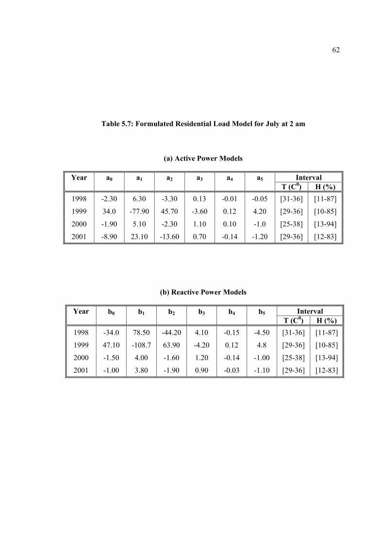
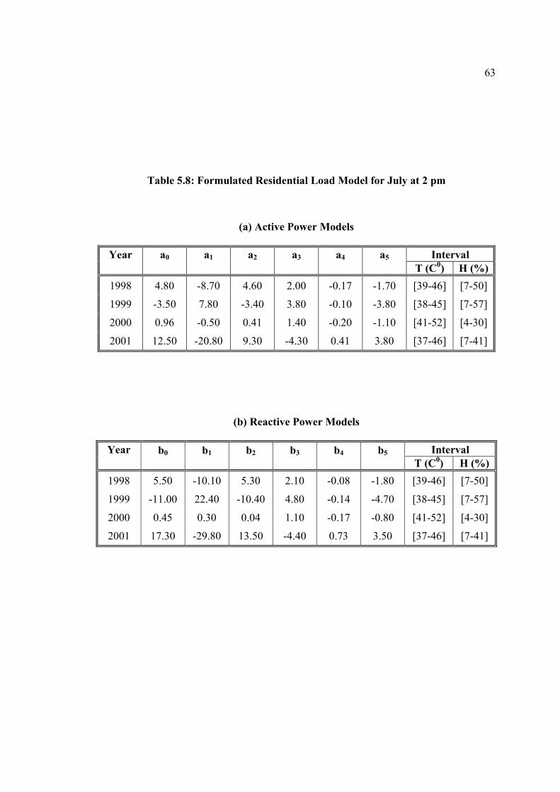
5.6.2 Residential Load Model for July
Tables 5.7 and 5.8 give the magnitude of the coefficients of the active and reactive
residential load models for July 2 am and 2 pm respectively.
The correlation between the magnitude of the active and reactive load model coefficients
for July models are different than for June models. The general trend of the magnitude of
the active and reactive load model coefficients for July 2 am are similar to those for July 2
pm. The temperature is reaching their maximum value in the summer period, it is 52
degree. Also, the humidity range in July is relatively higher than June.
It was noticed that the humidity coefficients (a3 & a4) for the active and reactive load
model for July are smaller compared to the other model coefficients. So, this gives
indication that the power demand influenced more by the temperature variation.
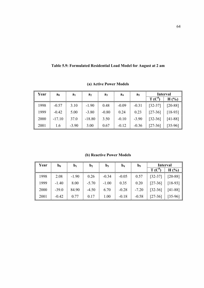
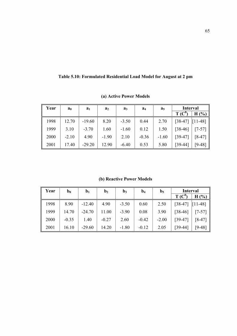
5.6.3 Residential Load Model for August
The magnitude of the coefficients of the active and reactive residential load models for
August 2 am and 2 pm are given in tables 5.9 and 5.10 respectively.
62
Table 5.7: Formulated Residential Load Model for July at 2 am
(a) Active Power Models
Year a0 a1 a2 a3 a4 a5 Interval T (C0) H (%)
1998 -2.30 6.30 -3.30 0.13 -0.01 -0.05 [31-36] [11-87]
1999 34.0 -77.90 45.70 -3.60 0.12 4.20 [29-36] [10-85]
2000 -1.90 5.10 -2.30 1.10 0.10 -1.0 [25-38] [13-94]
2001 -8.90 23.10 -13.60 0.70 -0.14 -1.20 [29-36] [12-83]
(b) Reactive Power Models
Year b0 b1 b2 b3 b4 b5 Interval T (C0) H (%)
1998 -34.0 78.50 -44.20 4.10 -0.15 -4.50 [31-36] [11-87]
1999 47.10 -108.7 63.90 -4.20 0.12 4.8 [29-36] [10-85]
2000 -1.50 4.00 -1.60 1.20 -0.14 -1.00 [25-38] [13-94]
2001 -1.00 3.80 -1.90 0.90 -0.03 -1.10 [29-36] [12-83]
63
Table 5.8: Formulated Residential Load Model for July at 2 pm
(a) Active Power Models
Year a0 a1 a2 a3 a4 a5 Interval T (C0) H (%)
1998 4.80 -8.70 4.60 2.00 -0.17 -1.70 [39-46] [7-50]
1999 -3.50 7.80 -3.40 3.80 -0.10 -3.80 [38-45] [7-57]
2000 0.96 -0.50 0.41 1.40 -0.20 -1.10 [41-52] [4-30]
2001 12.50 -20.80 9.30 -4.30 0.41 3.80 [37-46] [7-41]
(b) Reactive Power Models
Year b0 b1 b2 b3 b4 b5 Interval T (C0) H (%)
1998 5.50 -10.10 5.30 2.10 -0.08 -1.80 [39-46] [7-50]
1999 -11.00 22.40 -10.40 4.80 -0.14 -4.70 [38-45] [7-57]
2000 0.45 0.30 0.04 1.10 -0.17 -0.80 [41-52] [4-30]
2001 17.30 -29.80 13.50 -4.40 0.73 3.50 [37-46] [7-41]
64
Table 5.9: Formulated Residential Load Model for August at 2 am
(a) Active Power Models
Year a0 a1 a2 a3 a4 a5 Interval T (C0) H (%)
1998 -0.57 3.10 -1.90 0.48 -0.09 -0.31 [32-37] [20-88]
1999 -0.42 5.00 -3.80 -0.80 0.24 0.23 [27-36] [18-93]
2000 -17.10 37.0 -18.80 3.50 -0.10 -3.90 [32-36] [41-88]
2001 1.6 -3.90 3.00 0.67 -0.12 -0.36 [27-36] [35-96]
(b) Reactive Power Models
Year b0 b1 b2 b3 b4 b5 Interval T (C0) H (%)
1998 2.08 -1.90 0.26 -0.34 -0.05 0.57 [32-37] [20-88]
1999 -1.40 8.00 -5.70 -1.00 0.35 0.20 [27-36] [18-93]
2000 -39.0 84.90 -4.50 6.70 -0.28 -7.20 [32-36] [41-88]
2001 -0.42 0.77 0.17 1.00 -0.18 -0.58 [27-36] [35-96]
65
Table 5.10: Formulated Residential Load Model for August at 2 pm
(a) Active Power Models
Year a0 a1 a2 a3 a4 a5 Interval T (C0) H (%)
1998 12.70 -19.60 8.20 -3.50 0.44 2.70 [38-47] [11-48]
1999 3.10 -3.70 1.60 -1.60 0.12 1.50 [38-46] [7-57]
2000 -2.10 4.90 -1.90 2.10 -0.36 -1.60 [39-47] [8-47]
2001 17.40 -29.20 12.90 -6.40 0.53 5.80 [39-44] [9-48]
(b) Reactive Power Models
Year b0 b1 b2 b3 b4 b5 Interval T (C0) H (%)
1998 8.90 -12.40 4.90 -3.50 0.60 2.50 [38-47] [11-48]
1999 14.70 -24.70 11.00 -3.90 0.08 3.90 [38-46] [7-57]
2000 -0.35 1.40 -0.27 2.60 -0.42 -2.00 [39-47] [8-47]
2001 16.10 -29.60 14.20 -1.80 -0.12 2.05 [39-44] [9-48]

66
The temperatures during the August are varying from 27 to 37 degree at 2 am, while
during the 2 pm the variations are from 38 to 47 degree. However, the relative humidity is
reaching their maximum value during August at 2 am.
Also, it was noticed that the humidity coefficients (a3 & a4) for the active and reactive
load model for July are smaller compared to the other model coefficients. So, this gives
indication that the power demand influenced more by the temperature variation.
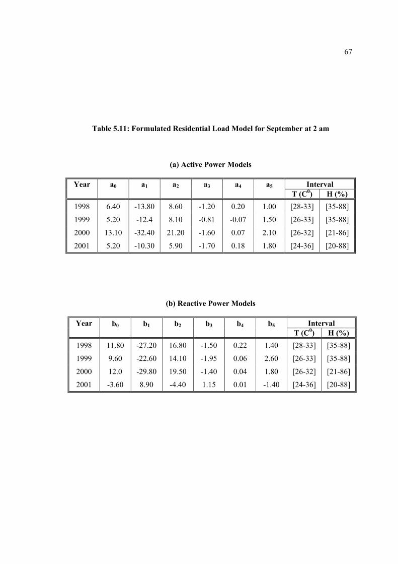
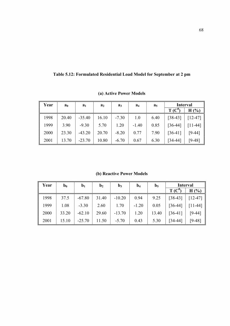
5.6.4 Residential Load Model for September
Tables 5.11 and 5.12 give the magnitude of the coefficients of the active and reactive
residential load models for September 2 am and 2 pm respectively.
The correlation between the magnitude of the active and reactive load model coefficients
for July models are similar to that for June models.
Generally, the magnitude of the active and reactive load model coefficients for September
2 pm are relatively higher than those for September 2 am. The temperatures are varying
from 24 to 36 degree at 2 am, whereas the variations at 2 pm are from 34 to 44 degree.
The temperature starts decreasing during September. However, the relative humidity is
also start decreasing in September varying from 20 to 88 percent at 2 am and varying
from 9 to 47 percent at 2 pm.
Also, it was noticed that the humidity coefficient a4 for the active and reactive load model
for July are smaller compared to the other model coefficients.
67
Table 5.11: Formulated Residential Load Model for September at 2 am
(a) Active Power Models
Year a0 a1 a2 a3 a4 a5 Interval T (C0) H (%)
1998 6.40 -13.80 8.60 -1.20 0.20 1.00 [28-33] [35-88]
1999 5.20 -12.4 8.10 -0.81 -0.07 1.50 [26-33] [35-88]
2000 13.10 -32.40 21.20 -1.60 0.07 2.10 [26-32] [21-86]
2001 5.20 -10.30 5.90 -1.70 0.18 1.80 [24-36] [20-88]
(b) Reactive Power Models
Year b0 b1 b2 b3 b4 b5 Interval T (C0) H (%)
1998 11.80 -27.20 16.80 -1.50 0.22 1.40 [28-33] [35-88]
1999 9.60 -22.60 14.10 -1.95 0.06 2.60 [26-33] [35-88]
2000 12.0 -29.80 19.50 -1.40 0.04 1.80 [26-32] [21-86]
2001 -3.60 8.90 -4.40 1.15 0.01 -1.40 [24-36] [20-88]
68
Table 5.12: Formulated Residential Load Model for September at 2 pm
(a) Active Power Models
Year a0 a1 a2 a3 a4 a5 Interval T (C0) H (%)
1998 20.40 -35.40 16.10 -7.30 1.0 6.40 [38-43] [12-47]
1999 3.90 -9.30 5.70 1.20 -1.40 0.85 [36-44] [11-44]
2000 23.30 -43.20 20.70 -8.20 0.77 7.90 [36-41] [9-44]
2001 13.70 -23.70 10.80 -6.70 0.67 6.30 [34-44] [9-48]
(b) Reactive Power Models
Year b0 b1 b2 b3 b4 b5 Interval T (C0) H (%)
1998 37.5 -67.80 31.40 -10.20 0.94 9.25 [38-43] [12-47]
1999 1.08 -3.30 2.60 1.70 -1.20 0.05 [36-44] [11-44]
2000 33.20 -62.10 29.60 -13.70 1.20 13.40 [36-41] [9-44]
2001 15.10 -25.70 11.50 -5.70 0.43 5.30 [34-44] [9-48]

69
5.7 Statistical Error Analysis
This section gives a statistical error analysis for the formulated residential load models for
June, July, August and September.
The statistical error analysis of the formulated residential load models involves two
aspects:
One is based on the calculation of the Mean absolute error (MAE), Standard
deviation errors (SDE) and variance value (VAR) for the active and reactive
power models.
The other aspect is based on plotting the error bars along the active and reactive
power.
Tables 5.13 to 5.16 give statistical error values for the four years models presented in the
previous section.
However, figures 5.3 to 5.10 show samples of the error bar plots for the active and
reactive power models for the month of August of the four year models at 2 pm. The rest
of the error bar plots for the active and reactive power models for the other months are
shown in the appendix C.

70
Table 5.13: Statistical Error analysis for June Models
(a) Time: 2 am
Statistical Error 1998 1999 2000 2001
P 0.0303 0.0369 0.0199 0.0212 MAE
Q 0.0356 0.0307 0.0243 0.0212
P 0.0371 0.0508 0.0310 0.0277 SDE
Q 0.0530 0.0390 0.0356 0.0306
P 0.0014 0.0026 0.0010 0.0008 VAR
Q 0.0028 0.0015 0.0013 0.0009
(b) Time: 2 pm
Statistical Error 1998 1999 2000 2001
P 0.0378 0.0385 0.0236 0.0183 MAE
Q 0.0544 0.0378 0.0258 0.0180
P 0.0527 0.0493 0.0337 0.0261 SDE
Q 0.0657 0.0502 0.0395 0.0229
P 0.0028 0.0024 0.0011 0.0007 VAR
Q 0.0043 0.0025 0.0016 0.0005

71
Table 5.14: Statistical Error analysis for July Models
(a) Time: 2 am
Statistical Error 1998 1999 2000 2001
P 0.0174 0.0611 0.0103 0.0223 MAE
Q 0.0252 0.0781 0.0165 0.0306
P 0.0217 0.0788 0.0122 0.0273 SDE
Q 0.0336 0.1035 0.0204 0.0411
P 0.0005 0.0062 0.0002 0.0008 VAR
Q 0.0011 0.0107 0.0004 0.0017
(b) Time: 2 pm
Statistical Error 1998 1999 2000 2001
P 0.0269 0.0269 0.0176 0.0197 MAE
Q 0.0203 0.0393 0.0221 0.0260
P 0.0372 0.0374 0.0216 0.0245 SDE
Q 0.0298 0.0496 0.0264 0.0309
P 0.0014 0.0014 0.0005 0.0006 VAR
Q 0.0009 0.0025 0.0007 0.0010
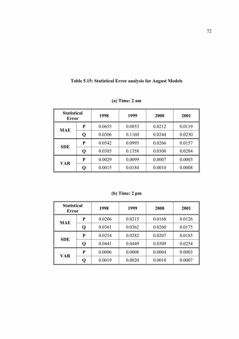
72
Table 5.15: Statistical Error analysis for August Models
(a) Time: 2 am
Statistical Error 1998 1999 2000 2001
P 0.0655 0.0853 0.0212 0.0119 MAE
Q 0.0306 0.1160 0.0244 0.0230
P 0.0542 0.0995 0.0266 0.0157 SDE
Q 0.0385 0.1358 0.0308 0.0284
P 0.0029 0.0099 0.0007 0.0003 VAR
Q 0.0015 0.0184 0.0010 0.0008
(b) Time: 2 pm
Statistical Error 1998 1999 2000 2001
P 0.0206 0.0215 0.0168 0.0126 MAE
Q 0.0361 0.0362 0.0260 0.0175
P 0.0254 0.0282 0.0207 0.0185 SDE
Q 0.0441 0.0449 0.0309 0.0254
P 0.0006 0.0008 0.0004 0.0003 VAR
Q 0.0019 0.0020 0.0010 0.0007
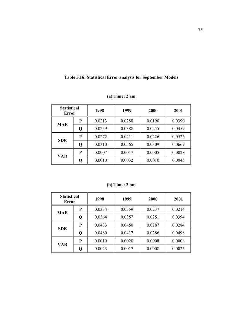
73
Table 5.16: Statistical Error analysis for September Models
(a) Time: 2 am
Statistical Error 1998 1999 2000 2001
P 0.0213 0.0288 0.0190 0.0390 MAE
Q 0.0259 0.0388 0.0255 0.0459
P 0.0272 0.0411 0.0226 0.0526 SDE
Q 0.0310 0.0565 0.0309 0.0669
P 0.0007 0.0017 0.0005 0.0028 VAR
Q 0.0010 0.0032 0.0010 0.0045
(b) Time: 2 pm
Statistical Error 1998 1999 2000 2001
P 0.0334 0.0359 0.0237 0.0214 MAE
Q 0.0364 0.0357 0.0251 0.0394
P 0.0433 0.0450 0.0287 0.0284 SDE
Q 0.0480 0.0417 0.0286 0.0498
P 0.0019 0.0020 0.0008 0.0008 VAR
Q 0.0023 0.0017 0.0008 0.0025
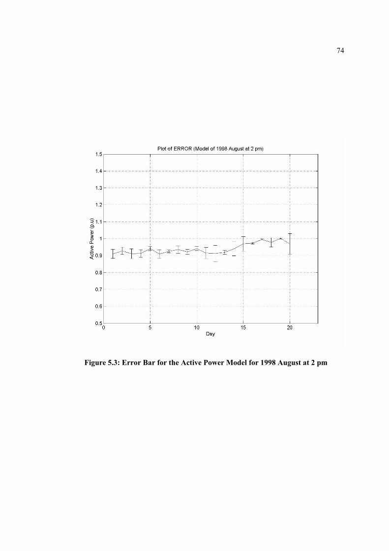
74
Figure 5.3: Error Bar for the Active Power Model for 1998 August at 2 pm

75
Figure 5.4: Error Bar for the Active Power Model for 1999 August at 2 pm
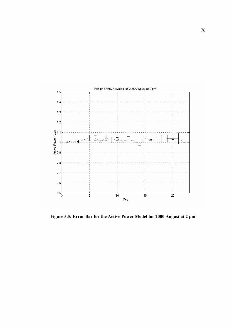
76
Figure 5.5: Error Bar for the Active Power Model for 2000 August at 2 pm
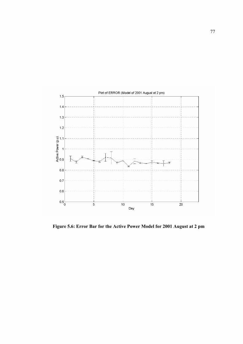
77
Figure 5.6: Error Bar for the Active Power Model for 2001 August at 2 pm
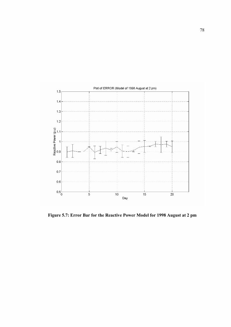
78
Figure 5.7: Error Bar for the Reactive Power Model for 1998 August at 2 pm
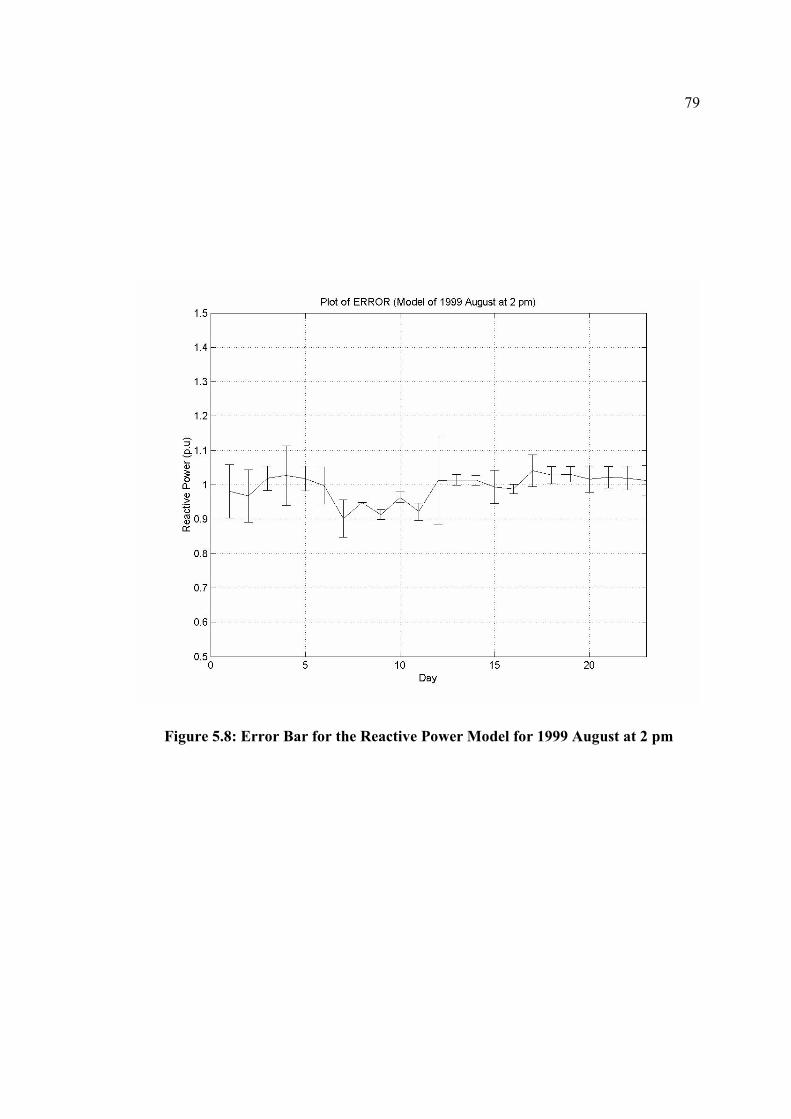
79
Figure 5.8: Error Bar for the Reactive Power Model for 1999 August at 2 pm

80
Figure 5.9: Error Bar for the Reactive Power Model for 2000 August at 2 pm
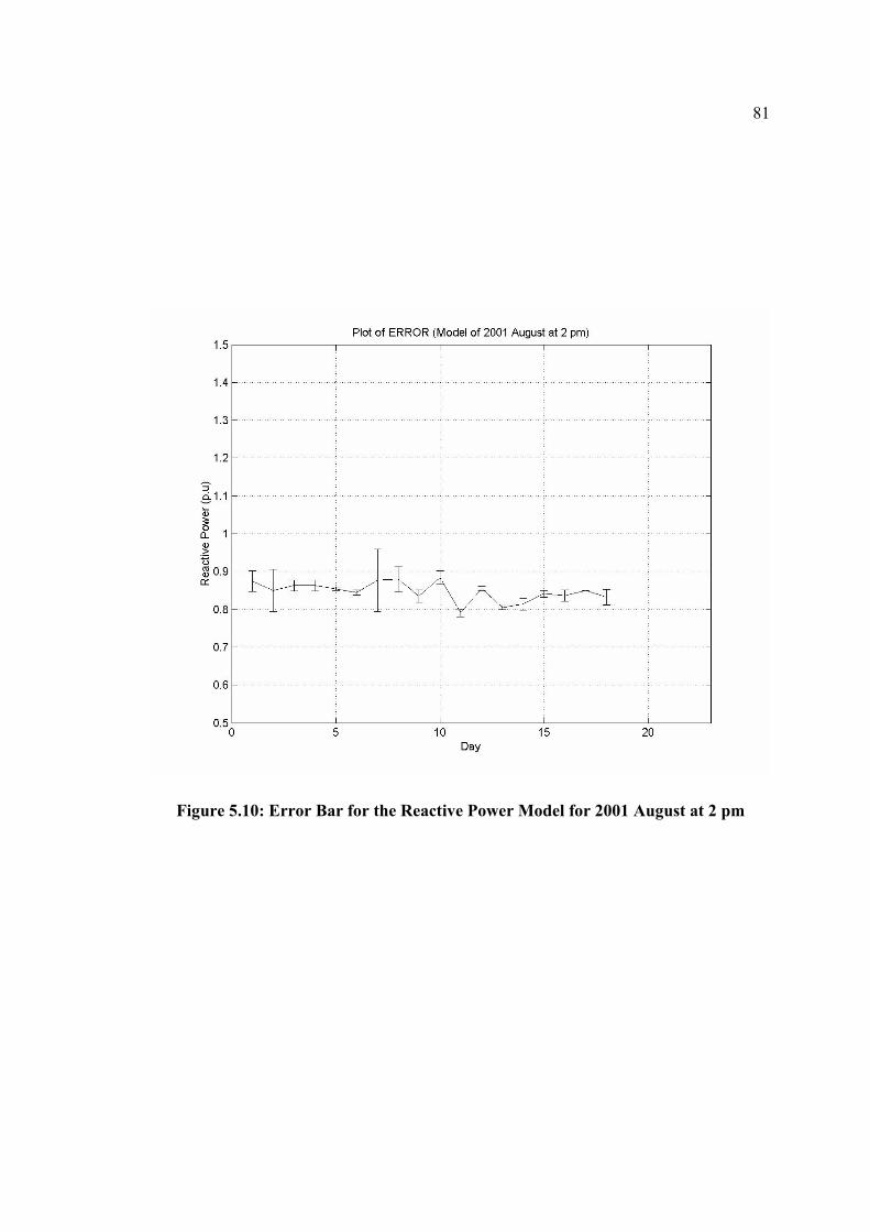
81
Figure 5.10: Error Bar for the Reactive Power Model for 2001 August at 2 pm

82
5.8 Forecasting Hourly Residential Load Demand
Electricity demand forecasts used in power system planning should be as accurate as
possible. The forecast is one of the major input parameters in developing future
generation, transmission and distribution facilities. Furthermore, it is also used to forecast
the utility's cash flow requirements, and thereby determine the prices of electricity. Any
substantial deviation in the forecast will result in either overbuilding of supply facilities,
or curtailment of demand.
This section discusses the current and the proposed approach for future residential load
forecasting.
5.8.1 Utility Current Approach
In developing the electricity demand forecast for the power system of the SEC-ERB, the
customer demand is segregated into various categories to reflect the mixture of
geographic grouping and large customer classes.
The SEC-ERB prepares a demand forecast each year to assess the additional capacity
requirements for generation, transmission and distribution facilities, and also to develop
the operation and investment plans. The present methodology places main emphasis on
the peak demand of the system. To develop the system peak demand forecast, a hybrid
analytical/judgmental approach is used to derive the maximum demand of each category
of customers. The customer classification is primarily by way of operating areas mainly
consisting of residential and commercial loads, while the oil industry and other large

83
industries are treated separately. The informations on demand growth in operating areas
are gathered from in-house data, while for oil and large industries are obtained through
power demand surveys. The system peak demand is then calculated by applying
coincidence factors to each customer group. [5, 6]
5.8.2 Weather Related Approach
Electricity demand estimates are the cornerstone of electricity operation and planning.
Without an adequate knowledge of the past and present electricity consumption patterns
and the likely future development, electricity operation and planning would be impossible.
In addition, load forecasting helps the utility to determine the system's spinning reserve, to
assess the fuel requirements, and to plan their unit maintenance scheduling. [6]
Residential load represent a high percentage of the total electric demand in the eastern
province of Saudi Arabia. Also, the residential load is highly influenced by weather
factors. Therefore, the residential load demand can be forecasted using the derived load
models. So, the power consumption can be forecasted using equation 5.7, whereas the
power can be calculated by using the previous year residential load model and the growth
rate of the current year.
NNNelN RateGrowthPPP )(1)1(mod ∗+= −− [5.7]
Where N is the current year need to be forecasted.

84
Let us illustrate this approach by forecasting the Agrabia substation load for year 2002
August at 2 pm.
The value of N is 2002 and the growth rate is 5.0 (source is utility). So, equation 5.7
becomes as follows:
20022001)2001(mod2002 )( RateGrowthPPP el ∗+= [5.8]
Figures 5.11 and 5.12 show the plots of the actual and forecasted values of active and
reactive power of August 2002 at 2pm for Agrabia substation.
The active and reactive power obtained from simulated results had shown the same shape
and trend of the actual one, but some differences are visible in their values.
Thus, the conclusion is that the derived load models can be used as another source to
forecast the residential load and to check the load value forecasted by the
analytical/judgmental approach which is used to derive the maximum demand.
Also, the approach presented in this thesis can be used for operational purpose where the
hourly and daily load forecasts are needed for many operational studies such as units
commitment and schedule outages of the equipment.

85
0
10
20
30
40
50
1 3 5 7 9 11 13 15 17 19
Day
Act
ive
Pow
er (
MW
)
Actual
Forecasted
Figure 5.11: Actual and Forecasted Active Power of Agrabia Substation for 2002
August at 2 pm
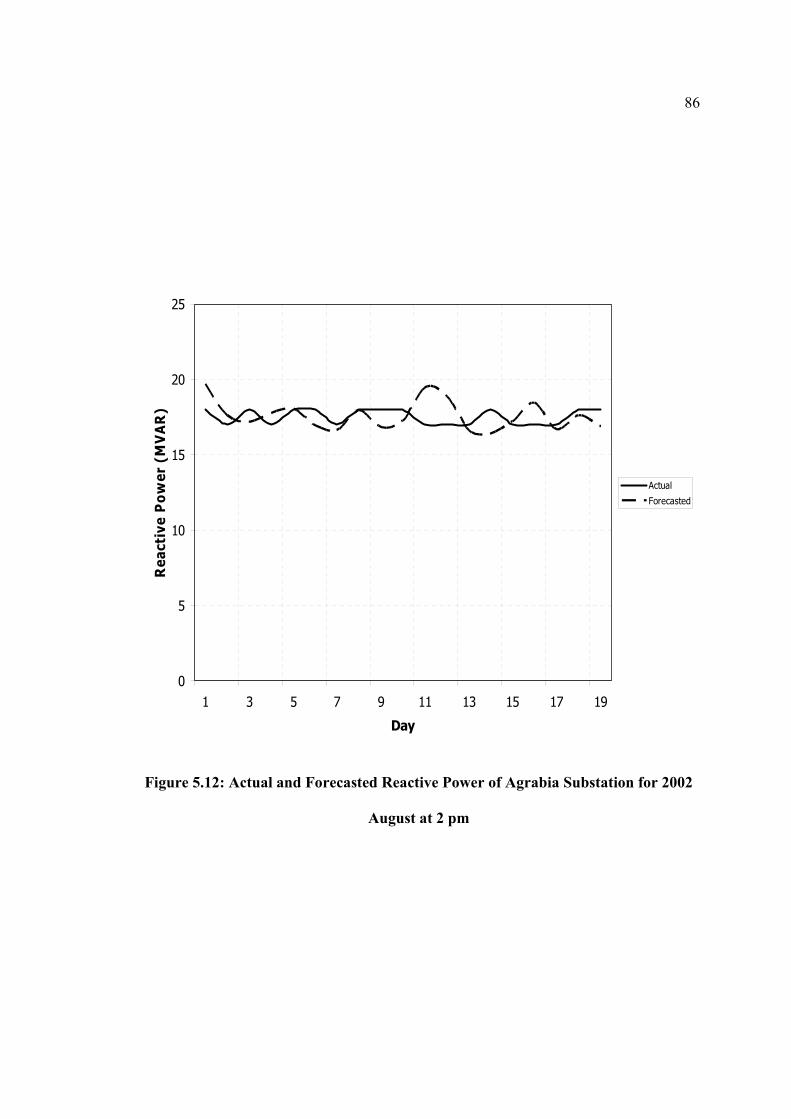
86
0
5
10
15
20
25
1 3 5 7 9 11 13 15 17 19
Day
Rea
ctiv
e P
ower
(M
VA
R)
Actual
Forecasted
Figure 5.12: Actual and Forecasted Reactive Power of Agrabia Substation for 2002
August at 2 pm

87
5.9 Test Load Model With New Substation
The formulated models can be used to forecast the load of any substation. This can easily
be done because of the normalized load models. So, the load can be forecasted by
identifying the normalized parameters of the new substation.
Let us illustrate this for another substation in the same area of Agrabia substation.
Bayonia substation is one of the grid stations in this area feeding residential load.
Therefore, using 2001 model load to predict the load for Bayonia substation for June 2 am
and August 2 pm respectively.
Figures 5.13 to 5.16 show the actual and predicted active and reactive power of Bayonia
substation for 2001models. The predicted power curves show same pattern and trend of
the actual ones. Also, the predicted active power are in a good agreement with actual
active power, where the reactive power have some significant differences in their values.
This is quite apparent in the error bar plots.
The error bar plots for the active and reactive power models for Bayonia substation are
shown in figures 5.17, 5.18, 5.19 and 5.20. The error bar plots for the active power
models are showing a reasonable error pattern. However, as mentioned in the previous
paragraph the reactive power results show big error range. This is due to the nature of the
reactive power where it is affected by the reactive compensation in the system.
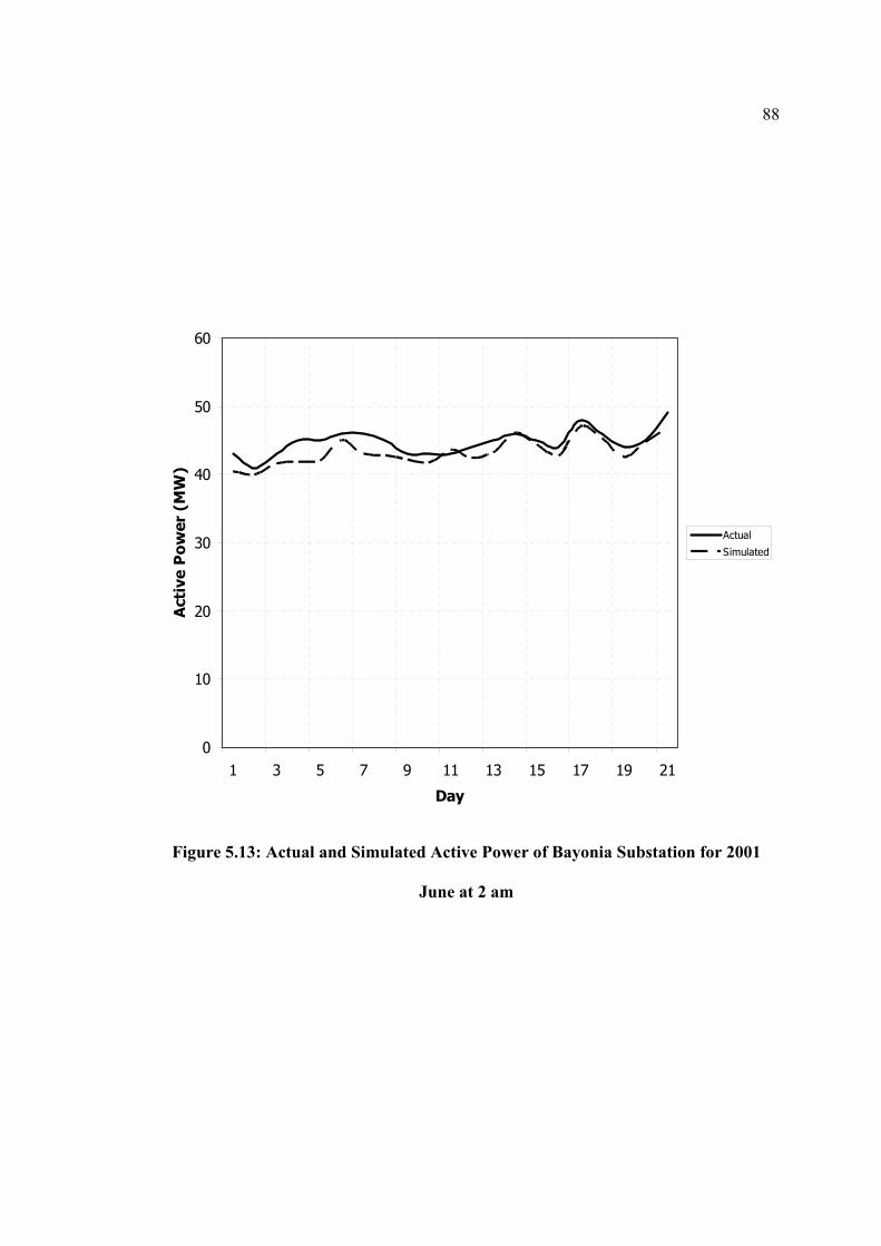
88
0
10
20
30
40
50
60
1 3 5 7 9 11 13 15 17 19 21
Day
Act
ive
Pow
er (
MW
)
Actual
Simulated
Figure 5.13: Actual and Simulated Active Power of Bayonia Substation for 2001
June at 2 am
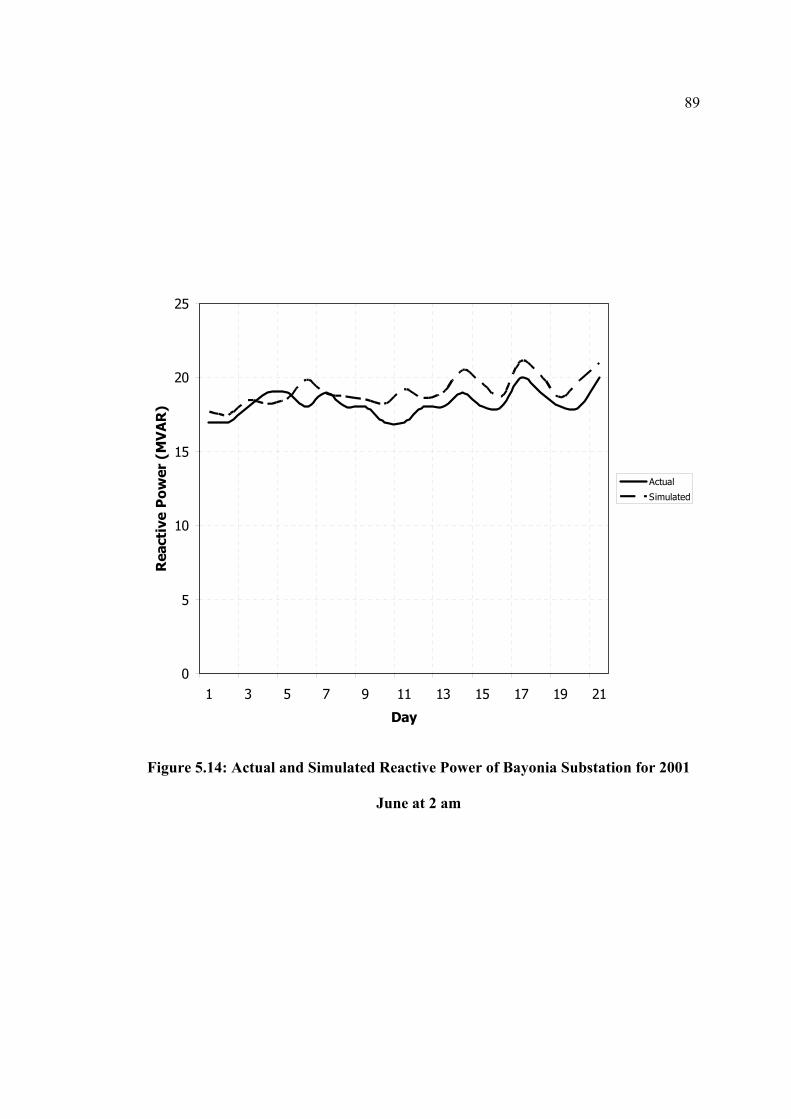
89
0
5
10
15
20
25
1 3 5 7 9 11 13 15 17 19 21
Day
Rea
ctiv
e P
ower
(M
VA
R)
Actual
Simulated
Figure 5.14: Actual and Simulated Reactive Power of Bayonia Substation for 2001
June at 2 am

90
0
10
20
30
40
50
60
1 3 5 7 9 11 13 15 17
Day
Act
ive
Pow
er (
MW
)
Actual
Simulated
Figure 5.15: Actual and Simulated Active Power of Bayonia Substation for 2001
August at 2 pm
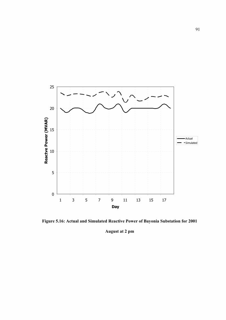
91
0
5
10
15
20
25
1 3 5 7 9 11 13 15 17
Day
Rea
ctve
Pow
er (
MV
AR
)
Actual
Simulated
Figure 5.16: Actual and Simulated Reactive Power of Bayonia Substation for 2001
August at 2 pm
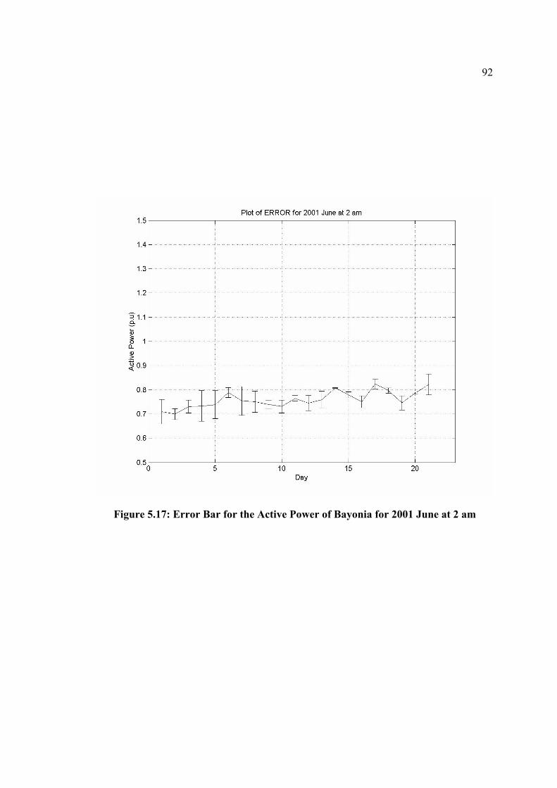
92
Figure 5.17: Error Bar for the Active Power of Bayonia for 2001 June at 2 am
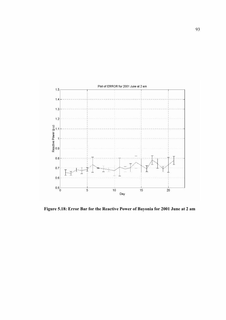
93
Figure 5.18: Error Bar for the Reactive Power of Bayonia for 2001 June at 2 am
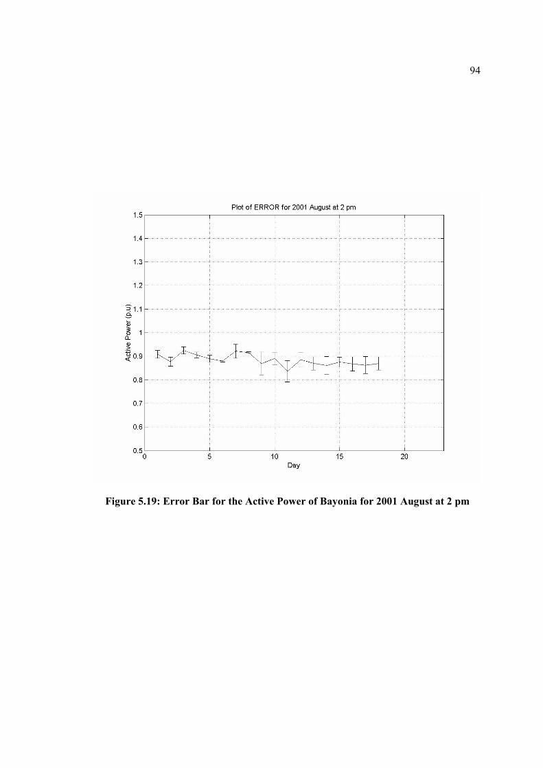
94
Figure 5.19: Error Bar for the Active Power of Bayonia for 2001 August at 2 pm
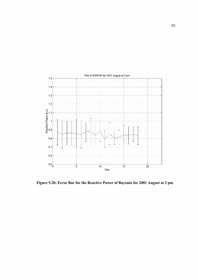
95
Figure 5.20: Error Bar for the Reactive Power of Bayonia for 2001 August at 2 pm

96
Chapter 6
CONCLUSIONS AND
RECOMMENDATIONS This chapter presents a summary of the work performed in this thesis. Also, it gives some
recommendations for future work.
6.1 Conclusions
In this thesis the load representation for static performance analysis was presented and
discussed.
Specific conclusions resulting from this work are as follows:
Year’s 1998 to 2002 measured data for highly hot and humid area at the eastern
province in Saudi Arabia data have been collected. Typical data for residential
load models has been selected from these data to reflect the impact of temperature
and relative humidity at steady voltage and at constant frequency.
96

97
The analysis, observations and investigations show four different modes of
weather conditions in summer period affect the power demand. These modes are
as follows:
- Mode1: High temperature with a moderate humidity will result in an
increasing power demand.
- Mode 2: Steady temperature with an increasing humidity will result in an
increasing power demand, but not sharp like mode one.
- Mode 3: High temperature with an increasing humidity will result in an
increasing power demand, but at up to a certain value where the humidity
moderate the temperature.
- Mode 4: Both of the temperature and the humidity are increasing. This will
result in a sharp increase in the power demand.
The parameters (coefficients) of the formulated residential load models were
identified by using the least squares fit technique in the MATLAB program.
The derived load models indicate that the relation of the temperature and the
relative humidity with load demand is a complex relation. It is a nonlinear relation.
Also, for different time of the day and the year there is a different behavior of the
load with respect to weather.
The load demand could be extracted on an hourly basis for residential load for
operational purposes.

98
The obtained fitting was tested and compared the measured load. They were in
good agreement. The analysis of the derived relations has shown behavior of the
load demand real and reactive as function of temperature and relative humidity.
6.2 Recommendations
There are a number of recommendations where further work can be done:
Since the collected data is measured at the bus feeding a diversified residential and
service load, a measured data taken, as input to a residence would reflect better
behavior.
Also, as extension to this work, it is good to repeat the same deriving load model
procedure done in this thesis to the Saudi Arabia Central Region where the system
peak demand is dominated by the residential demand that is mainly used for air
conditioning and is highly influenced by temperatures alone.
In the Gulf area air condition load represents high percentage of the residential
load in summer. So, determination of the dynamic behavior of air conditioner
using the component-based technique will give more accurate representation of the
residential load. Reference [16] describes techniques to derive the load models for
many home-heating appliances from field measurement.

99
APPENDICES

100
Appendix A
LOAD MODELING STRUCTURE
SELECTION
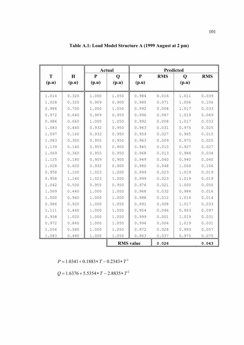
101
Table A.1: Load Model Structure A (1999 August at 2 pm)
Actual Predicted T H P Q P RMS Q RMS
(p.u) (p.u) (p.u) (p.u) (p.u) (p.u)
1.014 0.320 1.000 1.050 0.984 0.016 1.011 0.039
1.028 0.320 0.909 0.900 0.980 0.071 1.006 0.106
0.986 0.700 1.000 1.050 0.992 0.008 1.017 0.033
0.972 0.640 0.909 0.950 0.996 0.087 1.019 0.069
0.986 0.660 1.000 1.050 0.992 0.008 1.017 0.033
1.083 0.440 0.932 0.950 0.963 0.031 0.975 0.025
1.097 0.160 0.932 0.950 0.959 0.027 0.965 0.015
1.083 0.300 0.955 0.950 0.963 0.009 0.975 0.025
1.139 0.140 0.955 0.900 0.945 0.010 0.927 0.027
1.069 0.360 0.955 0.950 0.968 0.013 0.984 0.034
1.125 0.180 0.909 0.900 0.949 0.040 0.940 0.040
1.028 0.620 0.932 0.900 0.980 0.048 1.006 0.106
0.958 1.100 1.023 1.000 0.999 0.023 1.019 0.019
0.958 1.140 1.023 1.000 0.999 0.023 1.019 0.019
1.042 0.500 0.955 0.950 0.976 0.021 1.000 0.050
1.069 0.440 1.000 1.000 0.968 0.032 0.984 0.016
1.000 0.940 1.000 1.000 0.988 0.012 1.014 0.014
0.986 0.920 1.000 1.050 0.992 0.008 1.017 0.033
1.111 0.440 1.000 1.050 0.954 0.046 0.953 0.097
0.958 1.020 1.000 1.050 0.999 0.001 1.019 0.031
0.972 0.840 1.000 1.050 0.996 0.004 1.019 0.031
1.056 0.580 1.000 1.050 0.972 0.028 0.993 0.057
1.083 0.480 1.000 1.050 0.963 0.037 0.975 0.075
RMS value 0.026 0.043
22343.01883.00341.1 TTP ∗−∗+=
28835.25354.56376.1 TTQ ∗−∗+=
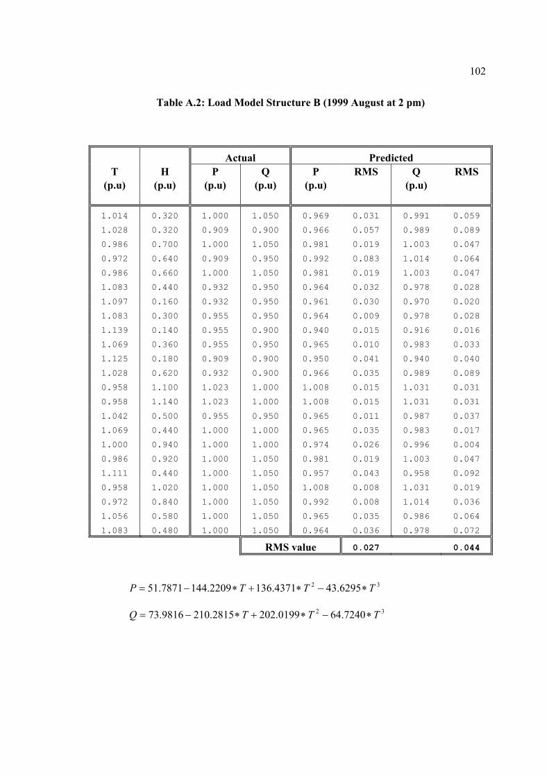
102
Table A.2: Load Model Structure B (1999 August at 2 pm)
Actual Predicted T H P Q P RMS Q RMS
(p.u) (p.u) (p.u) (p.u) (p.u) (p.u)
1.014 0.320 1.000 1.050 0.969 0.031 0.991 0.059
1.028 0.320 0.909 0.900 0.966 0.057 0.989 0.089
0.986 0.700 1.000 1.050 0.981 0.019 1.003 0.047
0.972 0.640 0.909 0.950 0.992 0.083 1.014 0.064
0.986 0.660 1.000 1.050 0.981 0.019 1.003 0.047
1.083 0.440 0.932 0.950 0.964 0.032 0.978 0.028
1.097 0.160 0.932 0.950 0.961 0.030 0.970 0.020
1.083 0.300 0.955 0.950 0.964 0.009 0.978 0.028
1.139 0.140 0.955 0.900 0.940 0.015 0.916 0.016
1.069 0.360 0.955 0.950 0.965 0.010 0.983 0.033
1.125 0.180 0.909 0.900 0.950 0.041 0.940 0.040
1.028 0.620 0.932 0.900 0.966 0.035 0.989 0.089
0.958 1.100 1.023 1.000 1.008 0.015 1.031 0.031
0.958 1.140 1.023 1.000 1.008 0.015 1.031 0.031
1.042 0.500 0.955 0.950 0.965 0.011 0.987 0.037
1.069 0.440 1.000 1.000 0.965 0.035 0.983 0.017
1.000 0.940 1.000 1.000 0.974 0.026 0.996 0.004
0.986 0.920 1.000 1.050 0.981 0.019 1.003 0.047
1.111 0.440 1.000 1.050 0.957 0.043 0.958 0.092
0.958 1.020 1.000 1.050 1.008 0.008 1.031 0.019
0.972 0.840 1.000 1.050 0.992 0.008 1.014 0.036
1.056 0.580 1.000 1.050 0.965 0.035 0.986 0.064
1.083 0.480 1.000 1.050 0.964 0.036 0.978 0.072
RMS value 0.027 0.044
32 6295.434371.1362209.1447871.51 TTTP ∗−∗+∗−=
32 7240.640199.2022815.2109816.73 TTTQ ∗−∗+∗−=
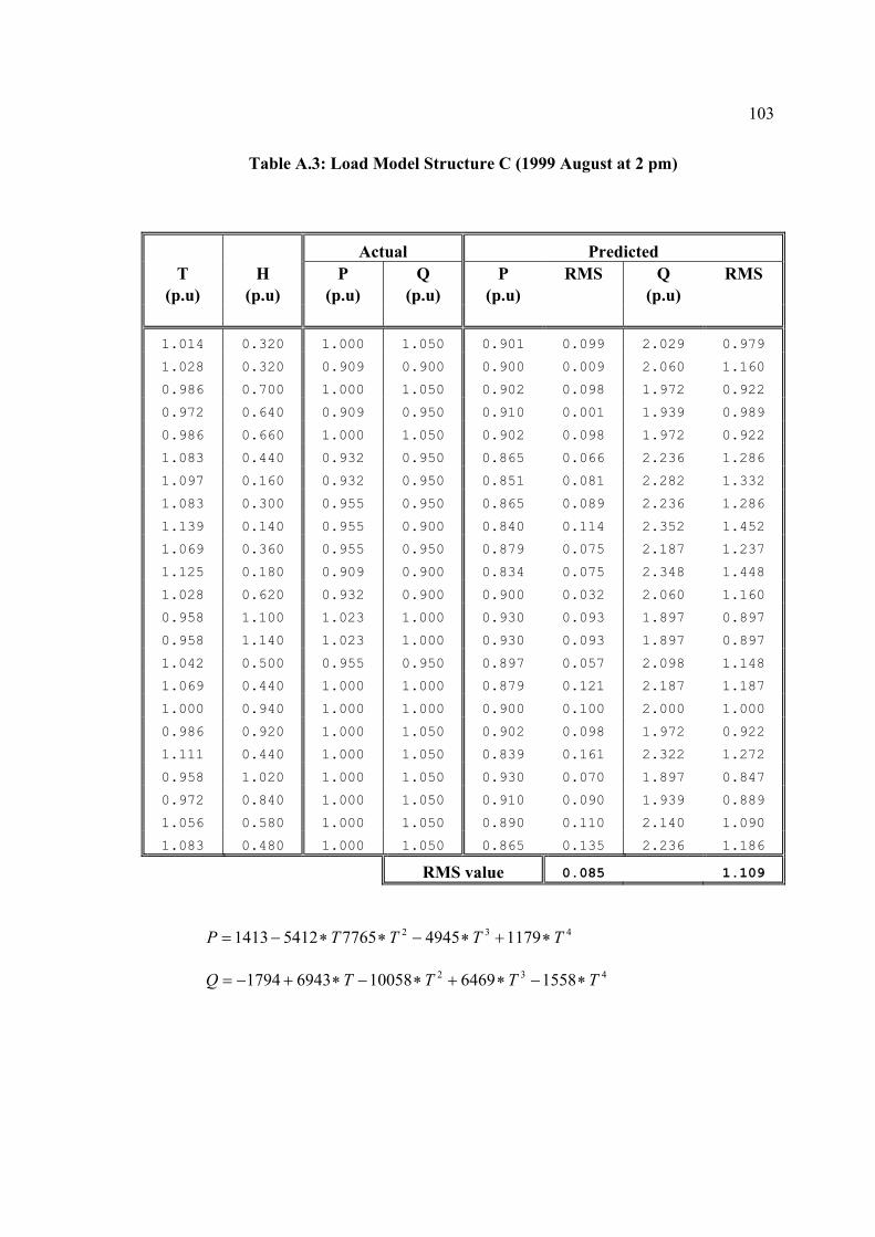
103
Table A.3: Load Model Structure C (1999 August at 2 pm)
Actual Predicted T H P Q P RMS Q RMS
(p.u) (p.u) (p.u) (p.u) (p.u) (p.u)
1.014 0.320 1.000 1.050 0.901 0.099 2.029 0.979
1.028 0.320 0.909 0.900 0.900 0.009 2.060 1.160
0.986 0.700 1.000 1.050 0.902 0.098 1.972 0.922
0.972 0.640 0.909 0.950 0.910 0.001 1.939 0.989
0.986 0.660 1.000 1.050 0.902 0.098 1.972 0.922
1.083 0.440 0.932 0.950 0.865 0.066 2.236 1.286
1.097 0.160 0.932 0.950 0.851 0.081 2.282 1.332
1.083 0.300 0.955 0.950 0.865 0.089 2.236 1.286
1.139 0.140 0.955 0.900 0.840 0.114 2.352 1.452
1.069 0.360 0.955 0.950 0.879 0.075 2.187 1.237
1.125 0.180 0.909 0.900 0.834 0.075 2.348 1.448
1.028 0.620 0.932 0.900 0.900 0.032 2.060 1.160
0.958 1.100 1.023 1.000 0.930 0.093 1.897 0.897
0.958 1.140 1.023 1.000 0.930 0.093 1.897 0.897
1.042 0.500 0.955 0.950 0.897 0.057 2.098 1.148
1.069 0.440 1.000 1.000 0.879 0.121 2.187 1.187
1.000 0.940 1.000 1.000 0.900 0.100 2.000 1.000
0.986 0.920 1.000 1.050 0.902 0.098 1.972 0.922
1.111 0.440 1.000 1.050 0.839 0.161 2.322 1.272
0.958 1.020 1.000 1.050 0.930 0.070 1.897 0.847
0.972 0.840 1.000 1.050 0.910 0.090 1.939 0.889
1.056 0.580 1.000 1.050 0.890 0.110 2.140 1.090
1.083 0.480 1.000 1.050 0.865 0.135 2.236 1.186
RMS value 0.085 1.109
432 11794945776554121413 TTTTP ∗+∗−∗∗−=
432 155864691005869431794 TTTTQ ∗−∗+∗−∗+−=
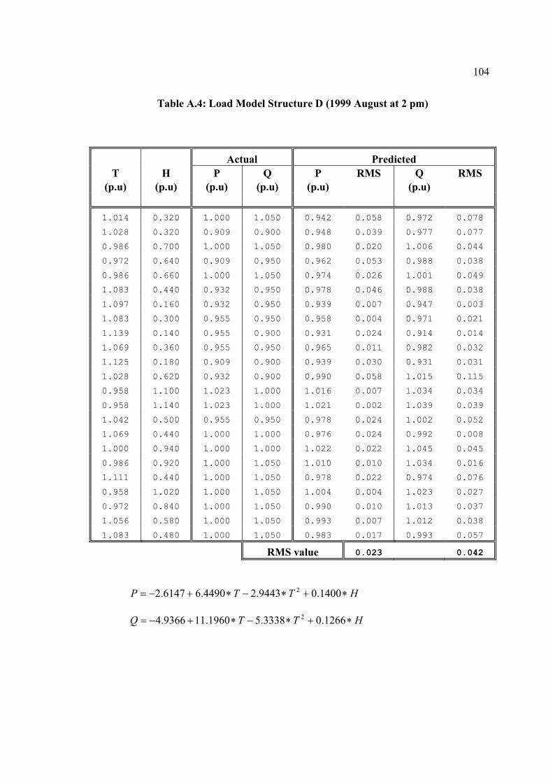
104
Table A.4: Load Model Structure D (1999 August at 2 pm)
Actual Predicted T H P Q P RMS Q RMS
(p.u) (p.u) (p.u) (p.u) (p.u) (p.u)
1.014 0.320 1.000 1.050 0.942 0.058 0.972 0.078
1.028 0.320 0.909 0.900 0.948 0.039 0.977 0.077
0.986 0.700 1.000 1.050 0.980 0.020 1.006 0.044
0.972 0.640 0.909 0.950 0.962 0.053 0.988 0.038
0.986 0.660 1.000 1.050 0.974 0.026 1.001 0.049
1.083 0.440 0.932 0.950 0.978 0.046 0.988 0.038
1.097 0.160 0.932 0.950 0.939 0.007 0.947 0.003
1.083 0.300 0.955 0.950 0.958 0.004 0.971 0.021
1.139 0.140 0.955 0.900 0.931 0.024 0.914 0.014
1.069 0.360 0.955 0.950 0.965 0.011 0.982 0.032
1.125 0.180 0.909 0.900 0.939 0.030 0.931 0.031
1.028 0.620 0.932 0.900 0.990 0.058 1.015 0.115
0.958 1.100 1.023 1.000 1.016 0.007 1.034 0.034
0.958 1.140 1.023 1.000 1.021 0.002 1.039 0.039
1.042 0.500 0.955 0.950 0.978 0.024 1.002 0.052
1.069 0.440 1.000 1.000 0.976 0.024 0.992 0.008
1.000 0.940 1.000 1.000 1.022 0.022 1.045 0.045
0.986 0.920 1.000 1.050 1.010 0.010 1.034 0.016
1.111 0.440 1.000 1.050 0.978 0.022 0.974 0.076
0.958 1.020 1.000 1.050 1.004 0.004 1.023 0.027
0.972 0.840 1.000 1.050 0.990 0.010 1.013 0.037
1.056 0.580 1.000 1.050 0.993 0.007 1.012 0.038
1.083 0.480 1.000 1.050 0.983 0.017 0.993 0.057
RMS value 0.023 0.042
HTTP ∗+∗−∗+−= 1400.09443.24490.66147.2 2
HTTQ ∗+∗−∗+−= 1266.03338.51960.119366.4 2
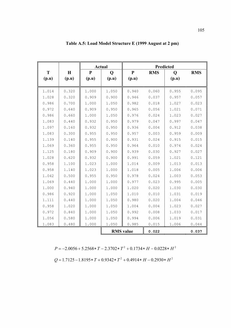
105
Table A.5: Load Model Structure E (1999 August at 2 pm)
Actual Predicted T H P Q P RMS Q RMS
(p.u) (p.u) (p.u) (p.u) (p.u) (p.u)
1.014 0.320 1.000 1.050 0.940 0.060 0.955 0.095
1.028 0.320 0.909 0.900 0.946 0.037 0.957 0.057
0.986 0.700 1.000 1.050 0.982 0.018 1.027 0.023
0.972 0.640 0.909 0.950 0.965 0.056 1.021 0.071
0.986 0.660 1.000 1.050 0.976 0.024 1.023 0.027
1.083 0.440 0.932 0.950 0.979 0.047 0.997 0.047
1.097 0.160 0.932 0.950 0.936 0.004 0.912 0.038
1.083 0.300 0.955 0.950 0.957 0.003 0.959 0.009
1.139 0.140 0.955 0.900 0.931 0.024 0.915 0.015
1.069 0.360 0.955 0.950 0.964 0.010 0.974 0.024
1.125 0.180 0.909 0.900 0.939 0.030 0.927 0.027
1.028 0.620 0.932 0.900 0.991 0.059 1.021 0.121
0.958 1.100 1.023 1.000 1.014 0.009 1.013 0.013
0.958 1.140 1.023 1.000 1.018 0.005 1.006 0.006
1.042 0.500 0.955 0.950 0.978 0.024 1.003 0.053
1.069 0.440 1.000 1.000 0.977 0.023 0.995 0.005
1.000 0.940 1.000 1.000 1.020 0.020 1.030 0.030
0.986 0.920 1.000 1.050 1.010 0.010 1.031 0.019
1.111 0.440 1.000 1.050 0.980 0.020 1.004 0.046
0.958 1.020 1.000 1.050 1.004 0.004 1.023 0.027
0.972 0.840 1.000 1.050 0.992 0.008 1.033 0.017
1.056 0.580 1.000 1.050 0.994 0.006 1.019 0.031
1.083 0.480 1.000 1.050 0.985 0.015 1.006 0.044
RMS value 0.022 0.037
22 0228.01734.03702.22568.50056.2 HHTTP ∗−∗+∗−∗+−=
22 2930.04914.09342.08195.17125.1 HHTTQ ∗−∗+∗+∗−=

106
Table A.6: Load Model Structure F (1999 August at 2 pm)
Actual Predicted T H P Q P RMS Q RMS
(p.u) (p.u) (p.u) (p.u) (p.u) (p.u)
1.014 0.320 1.000 1.050 0.941 0.059 0.954 0.096
1.028 0.320 0.909 0.900 0.947 0.038 0.955 0.055
0.986 0.700 1.000 1.050 0.981 0.019 1.028 0.022
0.972 0.640 0.909 0.950 0.965 0.056 1.020 0.070
0.986 0.660 1.000 1.050 0.976 0.024 1.024 0.026
1.083 0.440 0.932 0.950 0.980 0.048 0.996 0.046
1.097 0.160 0.932 0.950 0.934 0.002 0.915 0.035
1.083 0.300 0.955 0.950 0.958 0.003 0.958 0.008
1.139 0.140 0.955 0.900 0.930 0.025 0.917 0.017
1.069 0.360 0.955 0.950 0.965 0.011 0.973 0.023
1.125 0.180 0.909 0.900 0.938 0.029 0.928 0.028
1.028 0.620 0.932 0.900 0.990 0.058 1.023 0.123
0.958 1.100 1.023 1.000 1.015 0.008 1.011 0.011
0.958 1.140 1.023 1.000 1.020 0.002 1.002 0.002
1.042 0.500 0.955 0.950 0.979 0.024 1.003 0.053
1.069 0.440 1.000 1.000 0.977 0.023 0.993 0.007
1.000 0.940 1.000 1.000 1.018 0.018 1.035 0.035
0.986 0.920 1.000 1.050 1.008 0.008 1.035 0.015
1.111 0.440 1.000 1.050 0.982 0.018 1.001 0.049
0.958 1.020 1.000 1.050 1.004 0.004 1.024 0.026
0.972 0.840 1.000 1.050 0.990 0.010 1.035 0.015
1.056 0.580 1.000 1.050 0.994 0.006 1.020 0.030
1.083 0.480 1.000 1.050 0.985 0.015 1.005 0.045
RMS value 0.022 0.036
322 0546.01333.02318.01274.27458.47458.1 HHHTTP ∗+∗−∗∗−∗+−=
322 1054.00873.03786.04652.08324.02107.1 HHHTTQ ∗−∗−∗+∗+∗−=
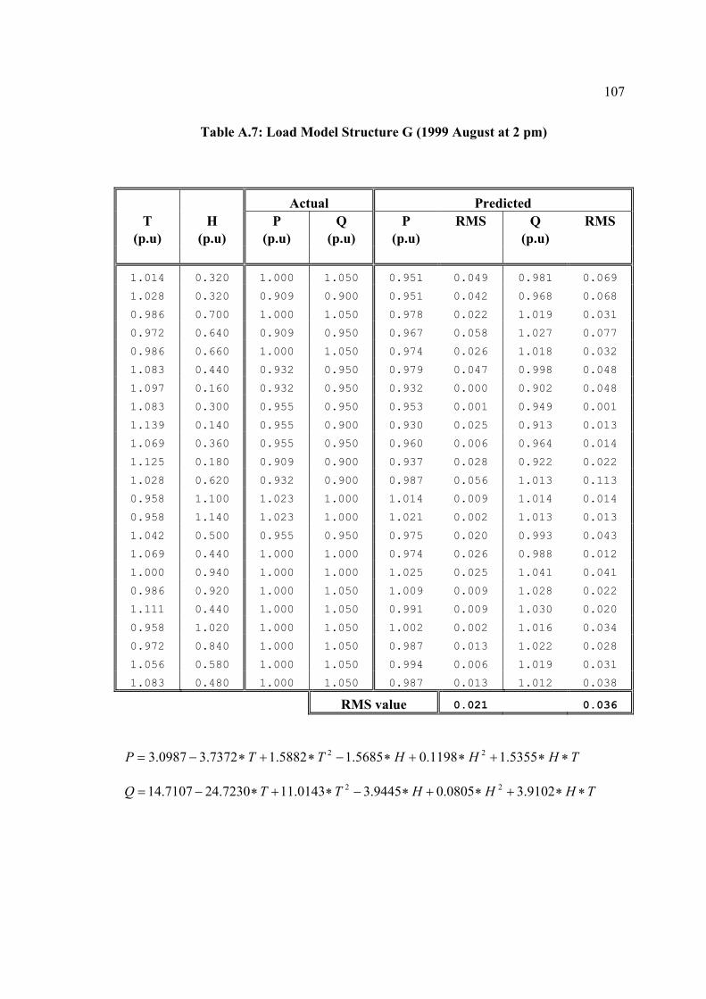
107
Table A.7: Load Model Structure G (1999 August at 2 pm)
Actual Predicted T H P Q P RMS Q RMS
(p.u) (p.u) (p.u) (p.u) (p.u) (p.u)
1.014 0.320 1.000 1.050 0.951 0.049 0.981 0.069
1.028 0.320 0.909 0.900 0.951 0.042 0.968 0.068
0.986 0.700 1.000 1.050 0.978 0.022 1.019 0.031
0.972 0.640 0.909 0.950 0.967 0.058 1.027 0.077
0.986 0.660 1.000 1.050 0.974 0.026 1.018 0.032
1.083 0.440 0.932 0.950 0.979 0.047 0.998 0.048
1.097 0.160 0.932 0.950 0.932 0.000 0.902 0.048
1.083 0.300 0.955 0.950 0.953 0.001 0.949 0.001
1.139 0.140 0.955 0.900 0.930 0.025 0.913 0.013
1.069 0.360 0.955 0.950 0.960 0.006 0.964 0.014
1.125 0.180 0.909 0.900 0.937 0.028 0.922 0.022
1.028 0.620 0.932 0.900 0.987 0.056 1.013 0.113
0.958 1.100 1.023 1.000 1.014 0.009 1.014 0.014
0.958 1.140 1.023 1.000 1.021 0.002 1.013 0.013
1.042 0.500 0.955 0.950 0.975 0.020 0.993 0.043
1.069 0.440 1.000 1.000 0.974 0.026 0.988 0.012
1.000 0.940 1.000 1.000 1.025 0.025 1.041 0.041
0.986 0.920 1.000 1.050 1.009 0.009 1.028 0.022
1.111 0.440 1.000 1.050 0.991 0.009 1.030 0.020
0.958 1.020 1.000 1.050 1.002 0.002 1.016 0.034
0.972 0.840 1.000 1.050 0.987 0.013 1.022 0.028
1.056 0.580 1.000 1.050 0.994 0.006 1.019 0.031
1.083 0.480 1.000 1.050 0.987 0.013 1.012 0.038
RMS value 0.021 0.036
THHHTTP ∗∗+∗+∗−∗+∗−= 5355.11198.05685.15882.17372.30987.3 22
THHHTTQ ∗∗+∗+∗−∗+∗−= 9102.30805.09445.30143.117230.247107.14 22
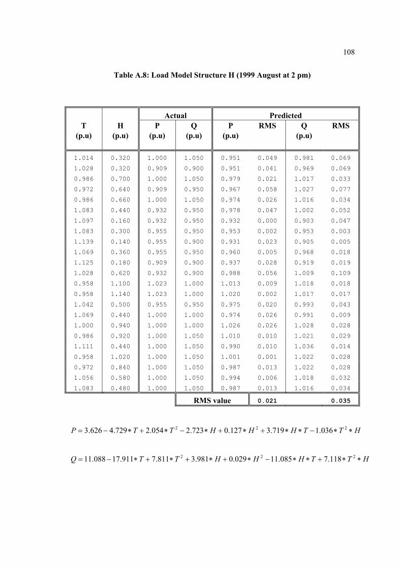
108
Table A.8: Load Model Structure H (1999 August at 2 pm)
Actual Predicted T H P Q P RMS Q RMS
(p.u) (p.u) (p.u) (p.u) (p.u) (p.u)
1.014 0.320 1.000 1.050 0.951 0.049 0.981 0.069
1.028 0.320 0.909 0.900 0.951 0.041 0.969 0.069
0.986 0.700 1.000 1.050 0.979 0.021 1.017 0.033
0.972 0.640 0.909 0.950 0.967 0.058 1.027 0.077
0.986 0.660 1.000 1.050 0.974 0.026 1.016 0.034
1.083 0.440 0.932 0.950 0.978 0.047 1.002 0.052
1.097 0.160 0.932 0.950 0.932 0.000 0.903 0.047
1.083 0.300 0.955 0.950 0.953 0.002 0.953 0.003
1.139 0.140 0.955 0.900 0.931 0.023 0.905 0.005
1.069 0.360 0.955 0.950 0.960 0.005 0.968 0.018
1.125 0.180 0.909 0.900 0.937 0.028 0.919 0.019
1.028 0.620 0.932 0.900 0.988 0.056 1.009 0.109
0.958 1.100 1.023 1.000 1.013 0.009 1.018 0.018
0.958 1.140 1.023 1.000 1.020 0.002 1.017 0.017
1.042 0.500 0.955 0.950 0.975 0.020 0.993 0.043
1.069 0.440 1.000 1.000 0.974 0.026 0.991 0.009
1.000 0.940 1.000 1.000 1.026 0.026 1.028 0.028
0.986 0.920 1.000 1.050 1.010 0.010 1.021 0.029
1.111 0.440 1.000 1.050 0.990 0.010 1.036 0.014
0.958 1.020 1.000 1.050 1.001 0.001 1.022 0.028
0.972 0.840 1.000 1.050 0.987 0.013 1.022 0.028
1.056 0.580 1.000 1.050 0.994 0.006 1.018 0.032
1.083 0.480 1.000 1.050 0.987 0.013 1.016 0.034
RMS value 0.021 0.035
HTTHHHTTP ∗∗−∗∗+∗+∗−∗+∗−= 222 036.1719.3127.0723.2054.2729.4626.3
HTTHHHTTQ ∗∗+∗∗−∗+∗+∗+∗−= 222 118.7085.11029.0981.3811.7911.17088.11
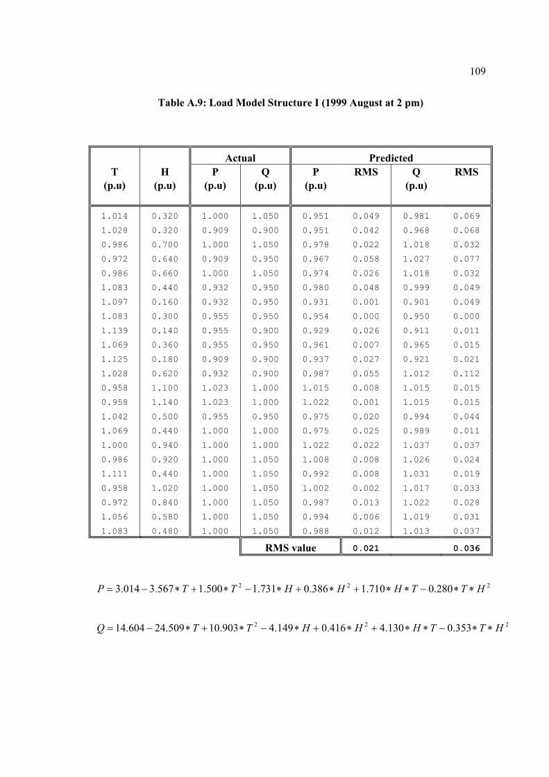
109
Table A.9: Load Model Structure I (1999 August at 2 pm)
Actual Predicted T H P Q P RMS Q RMS
(p.u) (p.u) (p.u) (p.u) (p.u) (p.u)
1.014 0.320 1.000 1.050 0.951 0.049 0.981 0.069
1.028 0.320 0.909 0.900 0.951 0.042 0.968 0.068
0.986 0.700 1.000 1.050 0.978 0.022 1.018 0.032
0.972 0.640 0.909 0.950 0.967 0.058 1.027 0.077
0.986 0.660 1.000 1.050 0.974 0.026 1.018 0.032
1.083 0.440 0.932 0.950 0.980 0.048 0.999 0.049
1.097 0.160 0.932 0.950 0.931 0.001 0.901 0.049
1.083 0.300 0.955 0.950 0.954 0.000 0.950 0.000
1.139 0.140 0.955 0.900 0.929 0.026 0.911 0.011
1.069 0.360 0.955 0.950 0.961 0.007 0.965 0.015
1.125 0.180 0.909 0.900 0.937 0.027 0.921 0.021
1.028 0.620 0.932 0.900 0.987 0.055 1.012 0.112
0.958 1.100 1.023 1.000 1.015 0.008 1.015 0.015
0.958 1.140 1.023 1.000 1.022 0.001 1.015 0.015
1.042 0.500 0.955 0.950 0.975 0.020 0.994 0.044
1.069 0.440 1.000 1.000 0.975 0.025 0.989 0.011
1.000 0.940 1.000 1.000 1.022 0.022 1.037 0.037
0.986 0.920 1.000 1.050 1.008 0.008 1.026 0.024
1.111 0.440 1.000 1.050 0.992 0.008 1.031 0.019
0.958 1.020 1.000 1.050 1.002 0.002 1.017 0.033
0.972 0.840 1.000 1.050 0.987 0.013 1.022 0.028
1.056 0.580 1.000 1.050 0.994 0.006 1.019 0.031
1.083 0.480 1.000 1.050 0.988 0.012 1.013 0.037
RMS value 0.021 0.036
222 280.0710.1386.0731.1500.1567.3014.3 HTTHHHTTP ∗∗−∗∗+∗+∗−∗+∗−=
222 353.0130.4416.0149.4903.10509.24604.14 HTTHHHTTQ ∗∗−∗∗+∗+∗−∗+∗−=
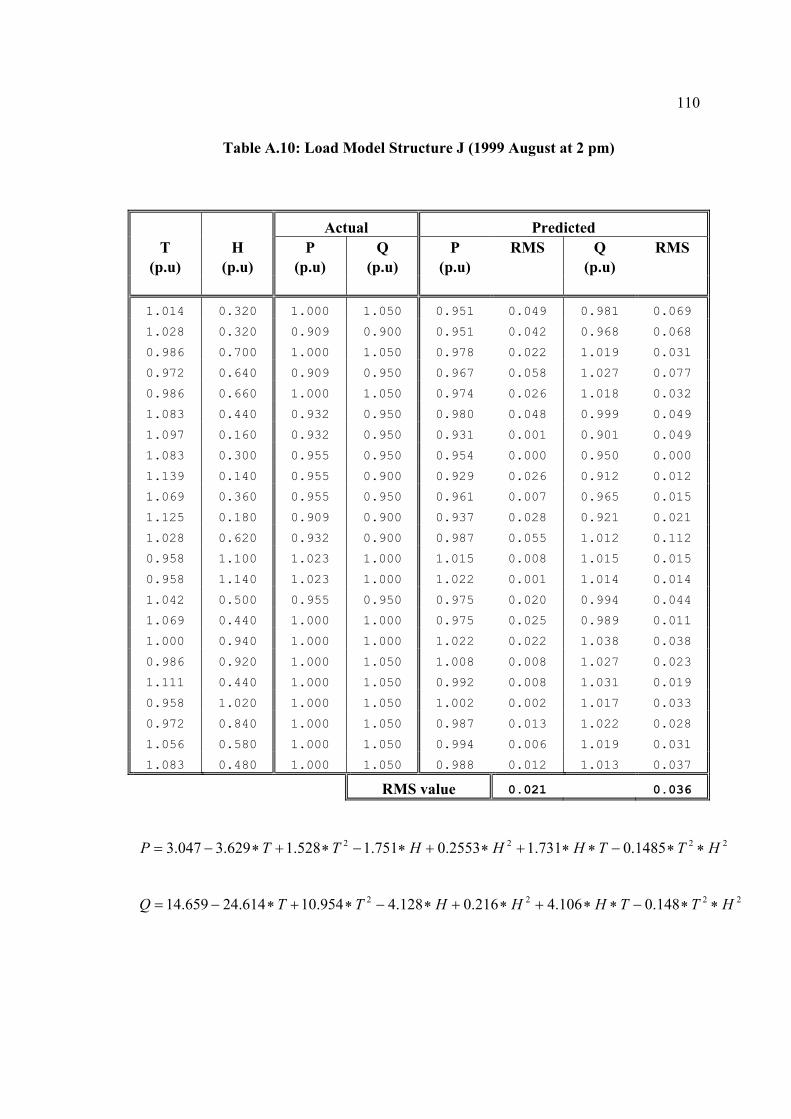
110
Table A.10: Load Model Structure J (1999 August at 2 pm)
Actual Predicted T H P Q P RMS Q RMS
(p.u) (p.u) (p.u) (p.u) (p.u) (p.u)
1.014 0.320 1.000 1.050 0.951 0.049 0.981 0.069
1.028 0.320 0.909 0.900 0.951 0.042 0.968 0.068
0.986 0.700 1.000 1.050 0.978 0.022 1.019 0.031
0.972 0.640 0.909 0.950 0.967 0.058 1.027 0.077
0.986 0.660 1.000 1.050 0.974 0.026 1.018 0.032
1.083 0.440 0.932 0.950 0.980 0.048 0.999 0.049
1.097 0.160 0.932 0.950 0.931 0.001 0.901 0.049
1.083 0.300 0.955 0.950 0.954 0.000 0.950 0.000
1.139 0.140 0.955 0.900 0.929 0.026 0.912 0.012
1.069 0.360 0.955 0.950 0.961 0.007 0.965 0.015
1.125 0.180 0.909 0.900 0.937 0.028 0.921 0.021
1.028 0.620 0.932 0.900 0.987 0.055 1.012 0.112
0.958 1.100 1.023 1.000 1.015 0.008 1.015 0.015
0.958 1.140 1.023 1.000 1.022 0.001 1.014 0.014
1.042 0.500 0.955 0.950 0.975 0.020 0.994 0.044
1.069 0.440 1.000 1.000 0.975 0.025 0.989 0.011
1.000 0.940 1.000 1.000 1.022 0.022 1.038 0.038
0.986 0.920 1.000 1.050 1.008 0.008 1.027 0.023
1.111 0.440 1.000 1.050 0.992 0.008 1.031 0.019
0.958 1.020 1.000 1.050 1.002 0.002 1.017 0.033
0.972 0.840 1.000 1.050 0.987 0.013 1.022 0.028
1.056 0.580 1.000 1.050 0.994 0.006 1.019 0.031
1.083 0.480 1.000 1.050 0.988 0.012 1.013 0.037
RMS value 0.021 0.036
2222 1485.0731.12553.0751.1528.1629.3047.3 HTTHHHTTP ∗∗−∗∗+∗+∗−∗+∗−=
2222 148.0106.4216.0128.4954.10614.24659.14 HTTHHHTTQ ∗∗−∗∗+∗+∗−∗+∗−=
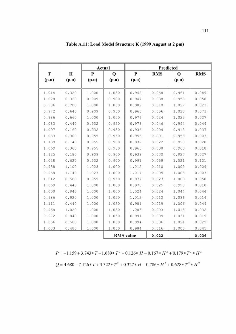
111
Table A.11: Load Model Structure K (1999 August at 2 pm)
Actual Predicted T H P Q P RMS Q RMS
(p.u) (p.u) (p.u) (p.u) (p.u) (p.u)
1.014 0.320 1.000 1.050 0.942 0.058 0.961 0.089
1.028 0.320 0.909 0.900 0.947 0.038 0.958 0.058
0.986 0.700 1.000 1.050 0.982 0.018 1.027 0.023
0.972 0.640 0.909 0.950 0.965 0.056 1.023 0.073
0.986 0.660 1.000 1.050 0.976 0.024 1.023 0.027
1.083 0.440 0.932 0.950 0.978 0.046 0.994 0.044
1.097 0.160 0.932 0.950 0.936 0.004 0.913 0.037
1.083 0.300 0.955 0.950 0.956 0.001 0.953 0.003
1.139 0.140 0.955 0.900 0.932 0.022 0.920 0.020
1.069 0.360 0.955 0.950 0.963 0.008 0.968 0.018
1.125 0.180 0.909 0.900 0.939 0.030 0.927 0.027
1.028 0.620 0.932 0.900 0.991 0.059 1.021 0.121
0.958 1.100 1.023 1.000 1.012 0.010 1.009 0.009
0.958 1.140 1.023 1.000 1.017 0.005 1.003 0.003
1.042 0.500 0.955 0.950 0.977 0.023 1.000 0.050
1.069 0.440 1.000 1.000 0.975 0.025 0.990 0.010
1.000 0.940 1.000 1.000 1.024 0.024 1.044 0.044
0.986 0.920 1.000 1.050 1.012 0.012 1.036 0.014
1.111 0.440 1.000 1.050 0.981 0.019 1.006 0.044
0.958 1.020 1.000 1.050 1.003 0.003 1.018 0.032
0.972 0.840 1.000 1.050 0.991 0.009 1.031 0.019
1.056 0.580 1.000 1.050 0.994 0.006 1.021 0.029
1.083 0.480 1.000 1.050 0.984 0.016 1.005 0.045
RMS value 0.022 0.036
2222 179.0167.0126.0689.1743.3159.1 HTHHTTP ∗∗+∗−∗+∗−∗+−=
2222 628.0786.0327.0322.3126.7680.4 HTHHTTQ ∗∗+∗−∗+∗+∗−=
112
Appendix B
DATA FOR LOAD MODELING

113
B.1 Original Raw Data
The mathematical models reported in this thesis are based on available measured data
which is a computerized database containing hourly data about generation, voltage,
frequency, load and weather for SEC-ERB utility in eastern province of Saudi Arabia.
These data are available from 1st January 1998 up to 31st December 2002.
The database files consist of three different files (CP, MS and M2). Each of these files
contains different kind of information for 24-hour a day. The contents of these files are as
follows:
CP - Substations Loads (MW & MVAR)
MS - Temperature
M2
- System Frequency
- Substation Voltage
- Relative Humidity
However, the data selected for residential load modeling derivation were extracted from
these files. So a program was made in excel sheet using Macro to extract the load
modeling data from the original raw data files.
The visual basic language was used to write the Macro program. Below are the program
written to extract the load data used in this thesis.
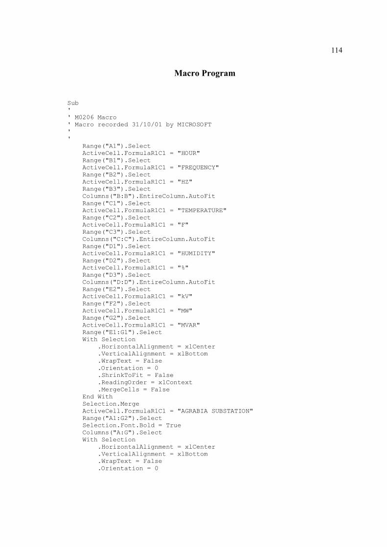
114
Macro Program Sub ' ' M0206 Macro ' Macro recorded 31/10/01 by MICROSOFT ' ' Range("A1").Select ActiveCell.FormulaR1C1 = "HOUR" Range("B1").Select ActiveCell.FormulaR1C1 = "FREQUENCY" Range("B2").Select ActiveCell.FormulaR1C1 = "HZ" Range("B3").Select Columns("B:B").EntireColumn.AutoFit Range("C1").Select ActiveCell.FormulaR1C1 = "TEMPERATURE" Range("C2").Select ActiveCell.FormulaR1C1 = "F" Range("C3").Select Columns("C:C").EntireColumn.AutoFit Range("D1").Select ActiveCell.FormulaR1C1 = "HUMIDITY" Range("D2").Select ActiveCell.FormulaR1C1 = "%" Range("D3").Select Columns("D:D").EntireColumn.AutoFit Range("E2").Select ActiveCell.FormulaR1C1 = "kV" Range("F2").Select ActiveCell.FormulaR1C1 = "MW" Range("G2").Select ActiveCell.FormulaR1C1 = "MVAR" Range("E1:G1").Select With Selection .HorizontalAlignment = xlCenter .VerticalAlignment = xlBottom .WrapText = False .Orientation = 0 .ShrinkToFit = False .ReadingOrder = xlContext .MergeCells = False End With Selection.Merge ActiveCell.FormulaR1C1 = "AGRABIA SUBSTATION" Range("A1:G2").Select Selection.Font.Bold = True Columns("A:G").Select With Selection .HorizontalAlignment = xlCenter .VerticalAlignment = xlBottom .WrapText = False .Orientation = 0
115
.ShrinkToFit = False .ReadingOrder = xlContext End With ' Enter the number of days Ndays = InputBox( _ prompt:="Please enter the # of Days 31,30,29,28.") ' LOOP 2002/06 For i = 1 To Ndays c = 3 + 24 * (i - 1) ' Cells(c, "A").Select ActiveCell.FormulaR1C1 = "1" Cells(c, "A").Select Selection.DataSeries Rowcol:=xlColumns, Type:=xlLinear, Date:=xlDay, _ Step:=1, Stop:=24, Trend:=False ' '====== Directory================== ChDir "D:\E\DATA\2002\06" '================================== If i = 1 Then M2day = "M2020601.DBF" ElseIf i = 2 Then M2day = "M2020602.DBF" ElseIf i = 3 Then M2day = "M2020603.DBF" ElseIf i = 4 Then M2day = "M2020604.DBF" ElseIf i = 5 Then M2day = "M2020605.DBF" ElseIf i = 6 Then M2day = "M2020606.DBF" ElseIf i = 7 Then M2day = "M2020607.DBF" ElseIf i = 8 Then M2day = "M2020608.DBF" ElseIf i = 9 Then M2day = "M2020609.DBF" ElseIf i = 10 Then M2day = "M2020610.DBF" ElseIf i = 11 Then M2day = "M2020611.DBF" ElseIf i = 12 Then M2day = "M2020612.DBF" ElseIf i = 13 Then M2day = "M2020613.DBF" ElseIf i = 14 Then M2day = "M2020614.DBF" ElseIf i = 15 Then M2day = "M2020615.DBF"
116
ElseIf i = 16 Then M2day = "M2020616.DBF" ElseIf i = 17 Then M2day = "M2020617.DBF" ElseIf i = 18 Then M2day = "M2020618.DBF" ElseIf i = 19 Then M2day = "M2020619.DBF" ElseIf i = 20 Then M2day = "M2020620.DBF" ElseIf i = 21 Then M2day = "M2020621.DBF" ElseIf i = 22 Then M2day = "M2020622.DBF" ElseIf i = 23 Then M2day = "M2020623.DBF" ElseIf i = 24 Then M2day = "M2020624.DBF" ElseIf i = 25 Then M2day = "M2020625.DBF" ElseIf i = 26 Then M2day = "M2020626.DBF" ElseIf i = 27 Then M2day = "M2020627.DBF" ElseIf i = 28 Then M2day = "M2020628.DBF" ElseIf i = 29 Then M2day = "M2020629.DBF" ElseIf i = 30 Then M2day = "M2020630.DBF" ElseIf i = 31 Then M2day = "M2020631.DBF" End If Workbooks.Open FileName:=M2day ActiveWindow.LargeScroll ToRight:=2 Cells.Find(What:="HZ", After:=ActiveCell, LookIn:=xlFormulas, LookAt:= _ xlPart, SearchOrder:=xlByRows, SearchDirection:=xlNext, MatchCase:=False).Activate ActiveWindow.ScrollColumn = 1 Range("A301:X301").Select Selection.Copy Windows("M0206").Activate Cells(c, "B").Select Selection.PasteSpecial Paste:=xlAll, Operation:=xlNone, SkipBlanks:=False _ , Transpose:=True Range("C11").Select Windows(M2day).Activate ActiveWindow.ScrollRow = 1 Range("I292").Select Application.CutCopyMode = False Cells.FindNext(After:=ActiveCell).Activate ActiveWindow.ScrollColumn = 1 Range("A1897:X1897").Select Selection.Copy Windows("M0206").Activate
117
Cells(c, "D").Select Selection.PasteSpecial Paste:=xlAll, Operation:=xlNone, SkipBlanks:=False _ , Transpose:=True Windows(M2day).Activate Range("D1889").Select Application.CutCopyMode = False Cells.Find(What:="AGRB-3-BUS1", After:=ActiveCell, LookIn:=xlFormulas, _ LookAt:=xlPart, SearchOrder:=xlByRows, SearchDirection:=xlNext, _ MatchCase:=False).Activate Range("AB1721:AC1724").Select Range("AC1721").Activate ActiveWindow.ScrollColumn = 1 ActiveWindow.ScrollColumn = 19 Range("Y1710").Select ActiveWindow.ScrollColumn = 1 Range("A1710:X1710").Select Selection.Copy Windows("M0206").Activate Cells(c, "E").Select Selection.PasteSpecial Paste:=xlAll, Operation:=xlNone, SkipBlanks:=False _ , Transpose:=True Windows(M2day).Activate Application.CutCopyMode = False Range("D1705").Select ActiveWindow.Close ' CP File If i = 1 Then CPday = "CP020601.DBF" ElseIf i = 2 Then CPday = "CP020602.DBF" ElseIf i = 3 Then CPday = "CP020603.DBF" ElseIf i = 4 Then CPday = "CP020604.DBF" ElseIf i = 5 Then CPday = "CP020605.DBF" ElseIf i = 6 Then CPday = "CP020606.DBF" ElseIf i = 7 Then CPday = "CP020607.DBF" ElseIf i = 8 Then CPday = "CP020608.DBF" ElseIf i = 9 Then CPday = "CP020609.DBF" ElseIf i = 10 Then CPday = "CP020610.DBF" ElseIf i = 11 Then CPday = "CP020611.DBF" ElseIf i = 12 Then CPday = "CP020612.DBF" ElseIf i = 13 Then
118
CPday = "CP020613.DBF" ElseIf i = 14 Then CPday = "CP020614.DBF" ElseIf i = 15 Then CPday = "CP020615.DBF" ElseIf i = 16 Then CPday = "CP020616.DBF" ElseIf i = 17 Then CPday = "CP020617.DBF" ElseIf i = 18 Then CPday = "CP020618.DBF" ElseIf i = 19 Then CPday = "CP020619.DBF" ElseIf i = 20 Then CPday = "CP020620.DBF" ElseIf i = 21 Then CPday = "CP020621.DBF" ElseIf i = 22 Then CPday = "CP020622.DBF" ElseIf i = 23 Then CPday = "CP020623.DBF" ElseIf i = 24 Then CPday = "CP020624.DBF" ElseIf i = 25 Then CPday = "CP020625.DBF" ElseIf i = 26 Then CPday = "CP020626.DBF" ElseIf i = 27 Then CPday = "CP020627.DBF" ElseIf i = 28 Then CPday = "CP020628.DBF" ElseIf i = 29 Then CPday = "CP020629.DBF" ElseIf i = 30 Then CPday = "CP020630.DBF" ElseIf i = 31 Then CPday = "CP020631.DBF" End If Workbooks.Open FileName:=CPday Cells.Find(What:="AGRABIA STATION", After:=ActiveCell, LookIn:=xlFormulas _ , LookAt:=xlPart, SearchOrder:=xlByRows, SearchDirection:=xlNext, _ MatchCase:=False).Activate ActiveWindow.SmallScroll ToRight:=-19 Range("A134:X134").Select Selection.Copy Windows("M0206").Activate Cells(c, "F").Select Selection.PasteSpecial Paste:=xlAll, Operation:=xlNone, SkipBlanks:=False _ , Transpose:=True Windows(CPday).Activate ActiveWindow.SmallScroll ToRight:=17 ActiveWindow.LargeScroll ToRight:=-2 Range("A135:X135").Select
119
Application.CutCopyMode = False Selection.Copy Windows("M0206").Activate Cells(c, "G").Select Selection.PasteSpecial Paste:=xlAll, Operation:=xlNone, SkipBlanks:=False _ , Transpose:=True Range("H11").Select Windows(CPday).Activate ActiveWindow.Close ' Ms File If i = 1 Then Msday = "Ms020601.DBF" ElseIf i = 2 Then Msday = "Ms020602.DBF" ElseIf i = 3 Then Msday = "Ms020603.DBF" ElseIf i = 4 Then Msday = "Ms020604.DBF" ElseIf i = 5 Then Msday = "Ms020605.DBF" ElseIf i = 6 Then Msday = "Ms020606.DBF" ElseIf i = 7 Then Msday = "Ms020607.DBF" ElseIf i = 8 Then Msday = "Ms020608.DBF" ElseIf i = 9 Then Msday = "Ms020609.DBF" ElseIf i = 10 Then Msday = "Ms020610.DBF" ElseIf i = 11 Then Msday = "Ms020611.DBF" ElseIf i = 12 Then Msday = "Ms020612.DBF" ElseIf i = 13 Then Msday = "Ms020613.DBF" ElseIf i = 14 Then Msday = "Ms020614.DBF" ElseIf i = 15 Then Msday = "Ms020615.DBF" ElseIf i = 16 Then Msday = "Ms020616.DBF" ElseIf i = 17 Then Msday = "Ms020617.DBF" ElseIf i = 18 Then Msday = "Ms020618.DBF" ElseIf i = 19 Then Msday = "Ms020619.DBF" ElseIf i = 20 Then Msday = "Ms020620.DBF" ElseIf i = 21 Then Msday = "Ms020621.DBF" ElseIf i = 22 Then Msday = "Ms020622.DBF"
120
ElseIf i = 23 Then Msday = "Ms020623.DBF" ElseIf i = 24 Then Msday = "Ms020624.DBF" ElseIf i = 25 Then Msday = "Ms020625.DBF" ElseIf i = 26 Then Msday = "Ms020626.DBF" ElseIf i = 27 Then Msday = "Ms020627.DBF" ElseIf i = 28 Then Msday = "Ms020628.DBF" ElseIf i = 29 Then Msday = "Ms020629.DBF" ElseIf i = 30 Then Msday = "Ms020630.DBF" ElseIf i = 31 Then Msday = "Ms020631.DBF" End If Workbooks.Open FileName:=Msday Cells.Find(What:="DAMTEMP_CT", After:=ActiveCell, LookIn:=xlFormulas, _ LookAt:=xlPart, SearchOrder:=xlByRows, SearchDirection:=xlNext, _ MatchCase:=False).Activate ActiveWindow.ScrollColumn = 1 Range("A602:X602").Select Selection.Copy Windows("M0206").Activate Cells(c, "C").Select Selection.PasteSpecial Paste:=xlAll, Operation:=xlNone, SkipBlanks:=False _ , Transpose:=True Windows(Msday).Activate ActiveWindow.Close Next i ' MODIFICATION ' Columns("A:G").Select With Selection .HorizontalAlignment = xlGeneral .VerticalAlignment = xlBottom .WrapText = False .Orientation = 0 .ShrinkToFit = False .ReadingOrder = xlContext End With With Selection .HorizontalAlignment = xlCenter .VerticalAlignment = xlBottom .WrapText = False .Orientation = 0 .ShrinkToFit = False .ReadingOrder = xlContext End With
121
Columns("D:D").Select Selection.Insert Shift:=xlToRight Range("C1:D1").Select With Selection .HorizontalAlignment = xlCenter .VerticalAlignment = xlBottom .WrapText = False .Orientation = 0 .ShrinkToFit = False .ReadingOrder = xlContext .MergeCells = False End With Selection.Merge Range("D2").Select ActiveCell.FormulaR1C1 = "C" Range("D3").Select ActiveCell.FormulaR1C1 = "=(RC[-1]-32)*5/9" Range("D3").Select Selection.Copy ' T = 3 + 24 * Ndays - 1 Range(Cells(4, "D"), Cells(T, "D")).Select ' Range("D4:D746").Select ActiveSheet.Paste Application.CutCopyMode = False Range("I10").Select ActiveWindow.SmallScroll Down:=13 ActiveWindow.ScrollRow = 1 ' MODIFICATION # 2 Range("I1").Select ActiveCell.FormulaR1C1 = "T" Range("I1").Select ActiveCell.FormulaR1C1 = "THETA" Range("I1").Select Selection.Font.Bold = True With Selection .HorizontalAlignment = xlCenter .VerticalAlignment = xlBottom .WrapText = False .Orientation = 0 .ShrinkToFit = False .ReadingOrder = xlContext .MergeCells = False End With Range("I3").Select ActiveCell.FormulaR1C1 = "=ATAN(RC[-1]/RC[-2])" Range("I3").Select Selection.Copy ' Range("I4:I746").Select Range(Cells(4, "I"), Cells(T, "I")).Select ActiveSheet.Paste ' CONDITION IF DIVID BY ZERO
122
For i = 3 To T If Cells(i, "H") = 0 Then Cells(i, "I") = 0 End If Next i Range("J20").Select Application.CutCopyMode = False ActiveWindow.SmallScroll Down:=1 ActiveWindow.ScrollRow = 725 ActiveWindow.ScrollRow = 1 Range("J1").Select ActiveCell.FormulaR1C1 = "P.F" Range("J1").Select Selection.Font.Bold = True With Selection .HorizontalAlignment = xlCenter .VerticalAlignment = xlBottom .WrapText = False .Orientation = 0 .ShrinkToFit = False .ReadingOrder = xlContext .MergeCells = False End With Range("J3").Select ActiveCell.FormulaR1C1 = "=COS(RC[-1])" Range("J3").Select Selection.Copy ' Range("J4:J746").Select Range(Cells(4, "J"), Cells(T, "J")).Select ActiveSheet.Paste For i = 3 To T If Cells(i, "J") = 1 Then Cells(i, "J") = 0 End If Next i Range("L4").Select ActiveWindow.ScrollRow = 725 ActiveWindow.ScrollRow = 1 Application.CutCopyMode = False Range("K1").Select ActiveCell.FormulaR1C1 = "CURRENT" Range("K2").Select ActiveCell.FormulaR1C1 = "A" Range("K1:K2").Select Selection.Font.Bold = True Columns("K:K").ColumnWidth = 8.57
123
Columns("K:K").EntireColumn.AutoFit Range("K3").Select ActiveCell.FormulaR1C1 = "=(RC[-4]/(1.73205*RC[-5]*RC[-1]))*1000" Range("K3").Select Selection.Copy ' Range("K4:K746").Select Range(Cells(4, "K"), Cells(T, "K")).Select ActiveSheet.Paste For i = 3 To T If Cells(i, "F") = 0 Then Cells(i, "K") = 0 End If If Cells(i, "H") = 0 Then Cells(i, "K") = 0 End If Next i Range("L19").Select ActiveWindow.SmallScroll Down:=0 Columns("I:K").Select Application.CutCopyMode = False Selection.NumberFormat = "0.0000" Columns("K:K").Select Selection.NumberFormat = "0.0" Columns("I:K").Select With Selection .HorizontalAlignment = xlGeneral .VerticalAlignment = xlBottom .WrapText = False .Orientation = 0 .ShrinkToFit = False .ReadingOrder = xlContext .MergeCells = False End With With Selection .HorizontalAlignment = xlCenter .VerticalAlignment = xlBottom .WrapText = False .Orientation = 0 .ShrinkToFit = False .ReadingOrder = xlContext .MergeCells = False End With Range("K11").Select Columns("I:I").Select Selection.EntireColumn.Hidden = True End Sub
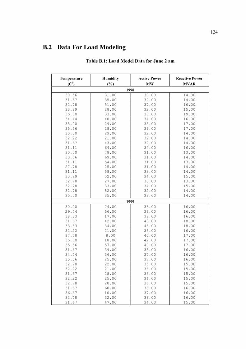
124
B.2 Data For Load Modeling
Table B.1: Load Model Data for June 2 am
Temperature Humidity Active Power Reactive Power (C0) (%) MW MVAR
1998 30.56 31.00 30.00 14.00 31.67 35.00 32.00 14.00 32.78 51.00 37.00 16.00 33.89 28.00 32.00 15.00 35.00 33.00 38.00 19.00 34.44 40.00 34.00 16.00 35.00 29.00 35.00 17.00 35.56 28.00 39.00 17.00 30.00 29.00 32.00 14.00 32.22 21.00 32.00 14.00 31.67 43.00 32.00 14.00 31.11 64.00 34.00 16.00 30.00 78.00 31.00 13.00 30.56 69.00 31.00 14.00 31.11 54.00 31.00 13.00 27.78 25.00 31.00 14.00 31.11 58.00 33.00 14.00 33.89 52.00 34.00 15.00 32.78 27.00 30.00 13.00 32.78 33.00 34.00 15.00 32.78 52.00 32.00 14.00 35.00 35.00 33.00 14.00
1999 30.00 74.00 38.00 16.00 29.44 56.00 38.00 16.00 38.33 17.00 39.00 16.00 31.67 42.00 43.00 18.00 33.33 34.00 43.00 18.00 32.22 21.00 38.00 16.00 37.78 8.00 40.00 17.00 35.00 18.00 42.00 17.00 35.56 57.00 40.00 17.00 31.67 39.00 38.00 16.00 34.44 36.00 37.00 16.00 35.56 25.00 37.00 16.00 32.78 22.00 35.00 15.00 32.22 21.00 36.00 15.00 31.67 28.00 36.00 15.00 32.22 25.00 36.00 15.00 32.78 20.00 36.00 15.00 31.67 60.00 38.00 16.00 36.67 10.00 37.00 16.00 32.78 32.00 38.00 16.00 31.67 47.00 34.00 15.00
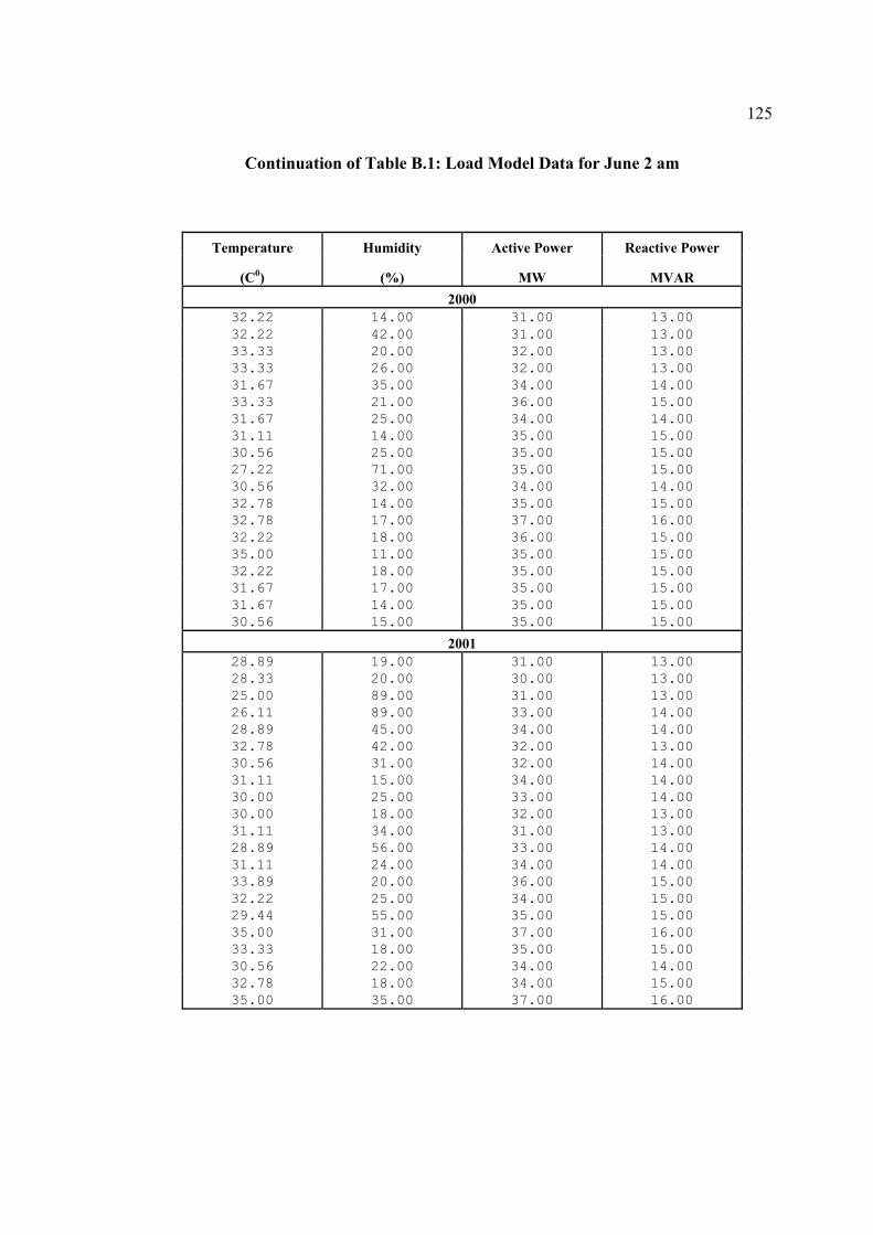
125
Continuation of Table B.1: Load Model Data for June 2 am
Temperature Humidity Active Power Reactive Power
(C0) (%) MW MVAR 2000
32.22 14.00 31.00 13.00 32.22 42.00 31.00 13.00 33.33 20.00 32.00 13.00 33.33 26.00 32.00 13.00 31.67 35.00 34.00 14.00 33.33 21.00 36.00 15.00 31.67 25.00 34.00 14.00 31.11 14.00 35.00 15.00 30.56 25.00 35.00 15.00 27.22 71.00 35.00 15.00 30.56 32.00 34.00 14.00 32.78 14.00 35.00 15.00 32.78 17.00 37.00 16.00 32.22 18.00 36.00 15.00 35.00 11.00 35.00 15.00 32.22 18.00 35.00 15.00 31.67 17.00 35.00 15.00 31.67 14.00 35.00 15.00 30.56 15.00 35.00 15.00
2001 28.89 19.00 31.00 13.00 28.33 20.00 30.00 13.00 25.00 89.00 31.00 13.00 26.11 89.00 33.00 14.00 28.89 45.00 34.00 14.00 32.78 42.00 32.00 13.00 30.56 31.00 32.00 14.00 31.11 15.00 34.00 14.00 30.00 25.00 33.00 14.00 30.00 18.00 32.00 13.00 31.11 34.00 31.00 13.00 28.89 56.00 33.00 14.00 31.11 24.00 34.00 14.00 33.89 20.00 36.00 15.00 32.22 25.00 34.00 15.00 29.44 55.00 35.00 15.00 35.00 31.00 37.00 16.00 33.33 18.00 35.00 15.00 30.56 22.00 34.00 14.00 32.78 18.00 34.00 15.00 35.00 35.00 37.00 16.00
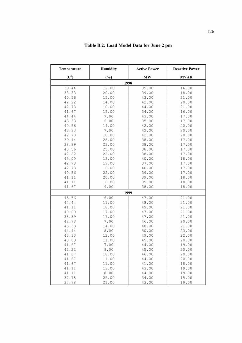
126
Table B.2: Load Model Data for June 2 pm
Temperature Humidity Active Power Reactive Power
(C0) (%) MW MVAR 1998
39.44 12.00 39.00 16.00 38.33 20.00 39.00 18.00 40.56 15.00 43.00 21.00 42.22 14.00 42.00 20.00 42.78 10.00 44.00 21.00 41.67 15.00 34.00 16.00 44.44 7.00 43.00 17.00 43.33 6.00 35.00 17.00 40.56 14.00 42.00 20.00 43.33 7.00 42.00 20.00 42.78 10.00 42.00 20.00 39.44 28.00 38.00 17.00 38.89 23.00 38.00 17.00 40.56 25.00 38.00 17.00 42.22 22.00 38.00 17.00 45.00 13.00 40.00 18.00 42.78 19.00 37.00 17.00 42.78 16.00 40.00 17.00 40.56 22.00 39.00 17.00 41.11 20.00 39.00 18.00 41.11 16.00 39.00 18.00 41.67 9.00 38.00 18.00
1999 45.56 6.00 47.00 21.00 44.44 11.00 48.00 21.00 41.11 18.00 49.00 21.00 40.00 17.00 47.00 21.00 38.89 17.00 47.00 21.00 42.78 7.00 46.00 20.00 43.33 14.00 48.00 21.00 44.44 8.00 50.00 23.00 43.33 12.00 49.00 22.00 40.00 11.00 45.00 20.00 41.67 7.00 44.00 19.00 42.22 8.00 45.00 20.00 41.67 18.00 46.00 20.00 41.67 11.00 44.00 20.00 41.67 11.00 41.00 18.00 41.11 13.00 43.00 19.00 41.11 8.00 44.00 19.00 37.78 25.00 34.00 15.00 37.78 21.00 43.00 19.00
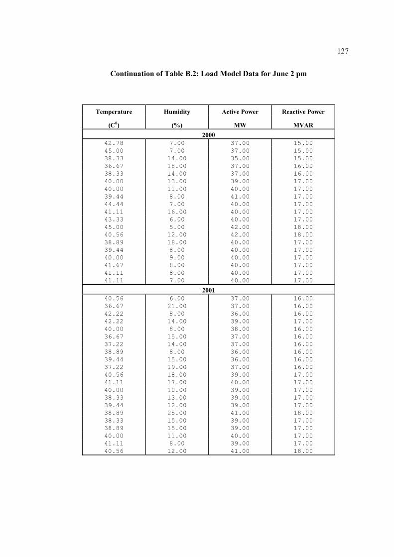
127
Continuation of Table B.2: Load Model Data for June 2 pm
Temperature Humidity Active Power Reactive Power
(C0) (%) MW MVAR 2000
42.78 7.00 37.00 15.00 45.00 7.00 37.00 15.00 38.33 14.00 35.00 15.00 36.67 18.00 37.00 16.00 38.33 14.00 37.00 16.00 40.00 13.00 39.00 17.00 40.00 11.00 40.00 17.00 39.44 8.00 41.00 17.00 44.44 7.00 40.00 17.00 41.11 16.00 40.00 17.00 43.33 6.00 40.00 17.00 45.00 5.00 42.00 18.00 40.56 12.00 42.00 18.00 38.89 18.00 40.00 17.00 39.44 8.00 40.00 17.00 40.00 9.00 40.00 17.00 41.67 8.00 40.00 17.00 41.11 8.00 40.00 17.00 41.11 7.00 40.00 17.00
2001 40.56 6.00 37.00 16.00 36.67 21.00 37.00 16.00 42.22 8.00 36.00 16.00 42.22 14.00 39.00 17.00 40.00 8.00 38.00 16.00 36.67 15.00 37.00 16.00 37.22 14.00 37.00 16.00 38.89 8.00 36.00 16.00 39.44 15.00 36.00 16.00 37.22 19.00 37.00 16.00 40.56 18.00 39.00 17.00 41.11 17.00 40.00 17.00 40.00 10.00 39.00 17.00 38.33 13.00 39.00 17.00 39.44 12.00 39.00 17.00 38.89 25.00 41.00 18.00 38.33 15.00 39.00 17.00 38.89 15.00 39.00 17.00 40.00 11.00 40.00 17.00 41.11 8.00 39.00 17.00 40.56 12.00 41.00 18.00
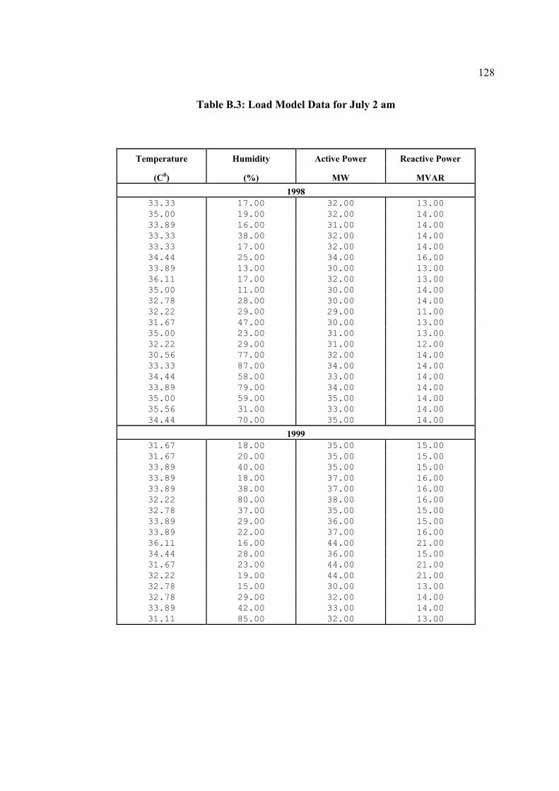
128
Table B.3: Load Model Data for July 2 am
Temperature Humidity Active Power Reactive Power
(C0) (%) MW MVAR 1998
33.33 17.00 32.00 13.00 35.00 19.00 32.00 14.00 33.89 16.00 31.00 14.00 33.33 38.00 32.00 14.00 33.33 17.00 32.00 14.00 34.44 25.00 34.00 16.00 33.89 13.00 30.00 13.00 36.11 17.00 32.00 13.00 35.00 11.00 30.00 14.00 32.78 28.00 30.00 14.00 32.22 29.00 29.00 11.00 31.67 47.00 30.00 13.00 35.00 23.00 31.00 13.00 32.22 29.00 31.00 12.00 30.56 77.00 32.00 14.00 33.33 87.00 34.00 14.00 34.44 58.00 33.00 14.00 33.89 79.00 34.00 14.00 35.00 59.00 35.00 14.00 35.56 31.00 33.00 14.00 34.44 70.00 35.00 14.00
1999 31.67 18.00 35.00 15.00 31.67 20.00 35.00 15.00 33.89 40.00 35.00 15.00 33.89 18.00 37.00 16.00 33.89 38.00 37.00 16.00 32.22 80.00 38.00 16.00 32.78 37.00 35.00 15.00 33.89 29.00 36.00 15.00 33.89 22.00 37.00 16.00 36.11 16.00 44.00 21.00 34.44 28.00 36.00 15.00 31.67 23.00 44.00 21.00 32.22 19.00 44.00 21.00 32.78 15.00 30.00 13.00 32.78 29.00 32.00 14.00 33.89 42.00 33.00 14.00 31.11 85.00 32.00 13.00
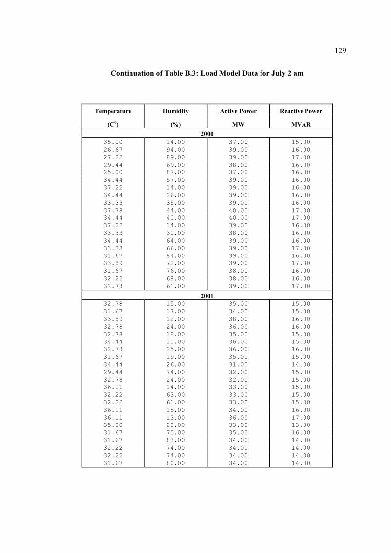
129
Continuation of Table B.3: Load Model Data for July 2 am
Temperature Humidity Active Power Reactive Power
(C0) (%) MW MVAR 2000
35.00 14.00 37.00 15.00 26.67 94.00 39.00 16.00 27.22 89.00 39.00 17.00 29.44 69.00 38.00 16.00 25.00 87.00 37.00 16.00 34.44 57.00 39.00 16.00 37.22 14.00 39.00 16.00 34.44 26.00 39.00 16.00 33.33 35.00 39.00 16.00 37.78 44.00 40.00 17.00 34.44 40.00 40.00 17.00 37.22 14.00 39.00 16.00 33.33 30.00 38.00 16.00 34.44 64.00 39.00 16.00 33.33 66.00 39.00 17.00 31.67 84.00 39.00 16.00 33.89 72.00 39.00 17.00 31.67 76.00 38.00 16.00 32.22 68.00 38.00 16.00 32.78 61.00 39.00 17.00
2001 32.78 15.00 35.00 15.00 31.67 17.00 34.00 15.00 33.89 12.00 38.00 16.00 32.78 24.00 36.00 16.00 32.78 18.00 35.00 15.00 34.44 15.00 36.00 15.00 32.78 25.00 36.00 16.00 31.67 19.00 35.00 15.00 34.44 26.00 31.00 14.00 29.44 74.00 32.00 15.00 32.78 24.00 32.00 15.00 36.11 14.00 33.00 15.00 32.22 63.00 33.00 15.00 32.22 61.00 33.00 15.00 36.11 15.00 34.00 16.00 36.11 13.00 36.00 17.00 35.00 20.00 33.00 13.00 31.67 75.00 35.00 16.00 31.67 83.00 34.00 14.00 32.22 74.00 34.00 14.00 32.22 74.00 34.00 14.00 31.67 80.00 34.00 14.00
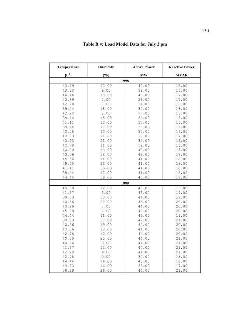
130
Table B.4: Load Model Data for July 2 pm
Temperature Humidity Active Power Reactive Power
(C0) (%) MW MVAR 1998
43.89 10.00 40.00 18.00 43.33 9.00 39.00 16.00 44.44 10.00 40.00 17.00 43.89 7.00 39.00 17.00 42.78 7.00 34.00 16.00 39.44 18.00 39.00 16.00 42.22 8.00 37.00 16.00 39.44 15.00 36.00 16.00 41.11 10.00 37.00 16.00 39.44 17.00 36.00 16.00 42.78 10.00 37.00 16.00 43.33 11.00 38.00 17.00 43.33 21.00 34.00 15.00 42.78 11.00 39.00 16.00 40.00 50.00 40.00 18.00 40.56 38.00 42.00 18.00 45.56 14.00 41.00 18.00 45.00 23.00 41.00 18.00 41.11 35.00 41.00 18.00 39.44 47.00 41.00 18.00 44.44 39.00 40.00 17.00
1999 40.00 12.00 43.00 19.00 41.67 8.00 43.00 19.00 38.33 33.00 44.00 19.00 40.56 27.00 45.00 20.00 43.89 7.00 44.00 20.00 45.00 7.00 46.00 20.00 44.44 11.00 43.00 19.00 38.33 57.00 47.00 21.00 40.56 19.00 44.00 20.00 40.56 18.00 44.00 20.00 42.78 12.00 44.00 20.00 40.00 25.00 44.00 21.00 40.56 9.00 44.00 21.00 41.67 12.00 44.00 21.00 42.22 9.00 44.00 21.00 42.78 9.00 39.00 18.00 44.44 14.00 40.00 18.00 43.33 16.00 39.00 17.00 38.89 26.00 44.00 21.00
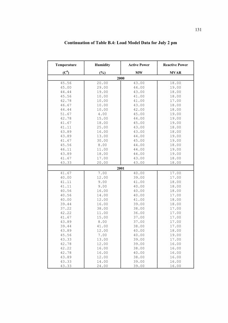
131
Continuation of Table B.4: Load Model Data for July 2 pm
Temperature Humidity Active Power Reactive Power
(C0) (%) MW MVAR 2000
45.56 20.00 43.00 18.00 45.00 29.00 44.00 19.00 44.44 19.00 43.00 18.00 45.56 10.00 41.00 18.00 42.78 10.00 41.00 17.00 46.67 10.00 43.00 18.00 44.44 10.00 42.00 18.00 51.67 4.00 45.00 19.00 42.78 15.00 44.00 19.00 41.67 18.00 45.00 19.00 41.11 25.00 43.00 18.00 43.89 16.00 43.00 18.00 43.89 13.00 44.00 19.00 41.67 30.00 45.00 19.00 45.56 8.00 44.00 18.00 46.11 11.00 44.00 19.00 43.89 18.00 44.00 19.00 41.67 17.00 43.00 18.00 43.33 20.00 43.00 18.00
2001 41.67 7.00 40.00 17.00 40.00 12.00 39.00 17.00 41.11 9.00 41.00 18.00 41.11 9.00 40.00 18.00 40.56 16.00 40.00 18.00 40.56 14.00 40.00 17.00 40.00 12.00 41.00 18.00 39.44 16.00 39.00 18.00 37.22 38.00 38.00 17.00 42.22 11.00 36.00 17.00 41.67 15.00 37.00 17.00 43.89 8.00 37.00 17.00 39.44 41.00 38.00 17.00 43.89 12.00 40.00 18.00 45.56 7.00 40.00 19.00 43.33 13.00 39.00 17.00 42.78 12.00 39.00 16.00 42.22 16.00 38.00 16.00 42.78 16.00 40.00 16.00 43.89 12.00 38.00 16.00 43.33 14.00 39.00 16.00 43.33 24.00 39.00 16.00
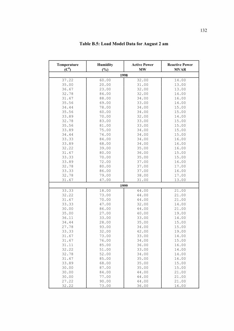
132
Table B.5: Load Model Data for August 2 am
Temperature Humidity Active Power Reactive Power (C0) (%) MW MVAR
1998 37.22 60.00 32.00 14.00 35.00 20.00 31.00 13.00 36.67 23.00 32.00 13.00 32.78 84.00 32.00 14.00 31.67 88.00 34.00 16.00 35.56 69.00 33.00 14.00 34.44 78.00 34.00 15.00 35.56 60.00 34.00 15.00 33.89 70.00 32.00 14.00 32.78 83.00 33.00 15.00 35.56 81.00 33.00 15.00 33.89 75.00 34.00 15.00 34.44 74.00 34.00 15.00 33.33 84.00 34.00 16.00 33.89 68.00 34.00 16.00 32.22 39.00 35.00 16.00 31.67 80.00 36.00 15.00 33.33 70.00 35.00 15.00 33.89 72.00 37.00 16.00 32.78 80.00 37.00 17.00 33.33 86.00 37.00 16.00 32.78 79.00 38.00 17.00 31.67 47.00 31.00 13.00
1999 33.33 18.00 44.00 21.00 32.22 73.00 44.00 21.00 31.67 70.00 44.00 21.00 33.33 47.00 32.00 14.00 30.00 86.00 44.00 21.00 35.00 27.00 40.00 19.00 36.11 33.00 33.00 14.00 34.44 28.00 35.00 15.00 27.78 93.00 34.00 15.00 33.33 32.00 42.00 19.00 31.67 73.00 33.00 14.00 31.67 76.00 34.00 15.00 31.11 85.00 36.00 16.00 32.22 51.00 33.00 14.00 32.78 52.00 34.00 14.00 31.67 85.00 35.00 16.00 33.89 68.00 35.00 15.00 30.00 87.00 35.00 15.00 30.00 84.00 44.00 21.00 30.00 77.00 44.00 21.00 27.22 90.00 44.00 21.00 32.22 73.00 36.00 16.00
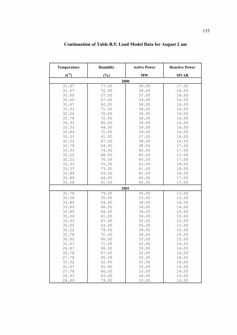
133
Continuation of Table B.5: Load Model Data for August 2 am
Temperature Humidity Active Power Reactive Power
(C0) (%) MW MVAR 2000
31.67 77.00 39.00 17.00 31.67 72.00 39.00 16.00 35.00 57.00 37.00 16.00 35.00 67.00 39.00 16.00 31.67 82.00 38.00 16.00 33.33 75.00 38.00 16.00 32.22 70.00 38.00 16.00 32.78 72.00 38.00 16.00 33.33 80.00 39.00 16.00 33.33 44.00 39.00 16.00 33.89 75.00 39.00 16.00 33.33 41.00 37.00 16.00 32.22 67.00 38.00 16.00 32.78 64.00 38.00 17.00 33.33 74.00 40.00 17.00 32.22 88.00 40.00 17.00 32.22 76.00 40.00 17.00 33.33 75.00 41.00 18.00 33.33 73.00 41.00 18.00 33.89 69.00 41.00 18.00 33.89 44.00 40.00 17.00 35.56 51.00 42.00 17.00
2001 32.78 79.00 34.00 13.00 35.56 35.00 33.00 13.00 33.89 59.00 34.00 14.00 33.89 68.00 34.00 14.00 33.89 64.00 34.00 15.00 35.00 61.00 34.00 15.00 33.33 87.00 35.00 15.00 35.00 54.00 35.00 15.00 32.22 79.00 34.00 15.00 32.78 72.00 34.00 15.00 30.00 86.00 33.00 15.00 31.67 75.00 32.00 14.00 26.67 96.00 33.00 14.00 32.78 87.00 32.00 14.00 27.78 85.00 33.00 14.00 32.22 52.00 31.00 14.00 31.67 92.00 33.00 14.00 27.78 80.00 33.00 14.00 28.33 83.00 34.00 15.00 28.89 79.00 33.00 14.00
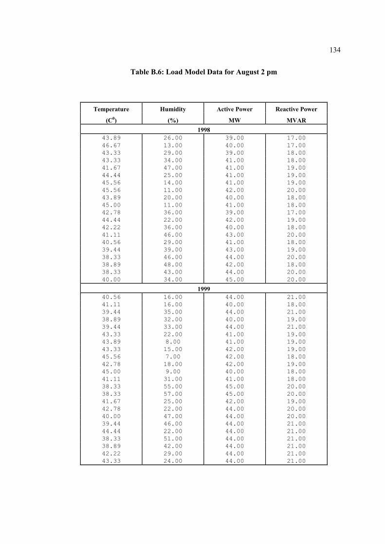
134
Table B.6: Load Model Data for August 2 pm
Temperature Humidity Active Power Reactive Power
(C0) (%) MW MVAR 1998
43.89 26.00 39.00 17.00 46.67 13.00 40.00 17.00 43.33 29.00 39.00 18.00 43.33 34.00 41.00 18.00 41.67 47.00 41.00 19.00 44.44 25.00 41.00 19.00 45.56 14.00 41.00 19.00 45.56 11.00 42.00 20.00 43.89 20.00 40.00 18.00 45.00 11.00 41.00 18.00 42.78 36.00 39.00 17.00 44.44 22.00 42.00 19.00 42.22 36.00 40.00 18.00 41.11 46.00 43.00 20.00 40.56 29.00 41.00 18.00 39.44 39.00 43.00 19.00 38.33 46.00 44.00 20.00 38.89 48.00 42.00 18.00 38.33 43.00 44.00 20.00 40.00 34.00 45.00 20.00
1999 40.56 16.00 44.00 21.00 41.11 16.00 40.00 18.00 39.44 35.00 44.00 21.00 38.89 32.00 40.00 19.00 39.44 33.00 44.00 21.00 43.33 22.00 41.00 19.00 43.89 8.00 41.00 19.00 43.33 15.00 42.00 19.00 45.56 7.00 42.00 18.00 42.78 18.00 42.00 19.00 45.00 9.00 40.00 18.00 41.11 31.00 41.00 18.00 38.33 55.00 45.00 20.00 38.33 57.00 45.00 20.00 41.67 25.00 42.00 19.00 42.78 22.00 44.00 20.00 40.00 47.00 44.00 20.00 39.44 46.00 44.00 21.00 44.44 22.00 44.00 21.00 38.33 51.00 44.00 21.00 38.89 42.00 44.00 21.00 42.22 29.00 44.00 21.00 43.33 24.00 44.00 21.00
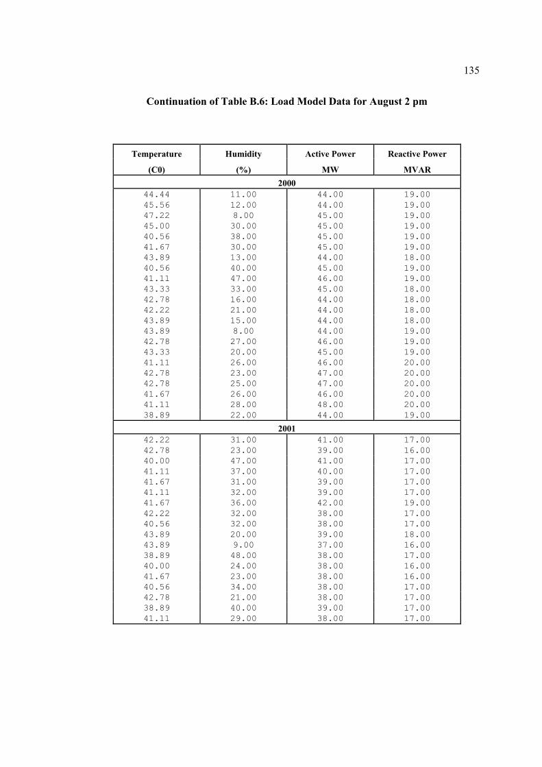
135
Continuation of Table B.6: Load Model Data for August 2 pm
Temperature Humidity Active Power Reactive Power
(C0) (%) MW MVAR 2000
44.44 11.00 44.00 19.00 45.56 12.00 44.00 19.00 47.22 8.00 45.00 19.00 45.00 30.00 45.00 19.00 40.56 38.00 45.00 19.00 41.67 30.00 45.00 19.00 43.89 13.00 44.00 18.00 40.56 40.00 45.00 19.00 41.11 47.00 46.00 19.00 43.33 33.00 45.00 18.00 42.78 16.00 44.00 18.00 42.22 21.00 44.00 18.00 43.89 15.00 44.00 18.00 43.89 8.00 44.00 19.00 42.78 27.00 46.00 19.00 43.33 20.00 45.00 19.00 41.11 26.00 46.00 20.00 42.78 23.00 47.00 20.00 42.78 25.00 47.00 20.00 41.67 26.00 46.00 20.00 41.11 28.00 48.00 20.00 38.89 22.00 44.00 19.00
2001 42.22 31.00 41.00 17.00 42.78 23.00 39.00 16.00 40.00 47.00 41.00 17.00 41.11 37.00 40.00 17.00 41.67 31.00 39.00 17.00 41.11 32.00 39.00 17.00 41.67 36.00 42.00 19.00 42.22 32.00 38.00 17.00 40.56 32.00 38.00 17.00 43.89 20.00 39.00 18.00 43.89 9.00 37.00 16.00 38.89 48.00 38.00 17.00 40.00 24.00 38.00 16.00 41.67 23.00 38.00 16.00 40.56 34.00 38.00 17.00 42.78 21.00 38.00 17.00 38.89 40.00 39.00 17.00 41.11 29.00 38.00 17.00
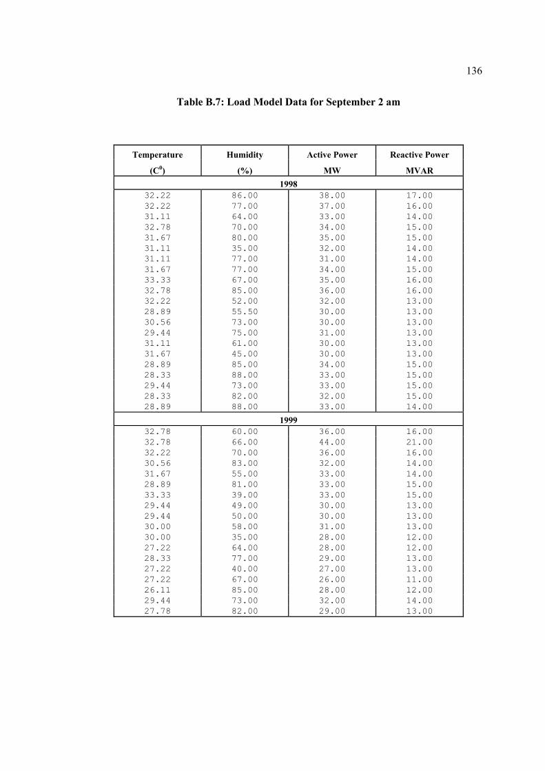
136
Table B.7: Load Model Data for September 2 am
Temperature Humidity Active Power Reactive Power
(C0) (%) MW MVAR 1998
32.22 86.00 38.00 17.00 32.22 77.00 37.00 16.00 31.11 64.00 33.00 14.00 32.78 70.00 34.00 15.00 31.67 80.00 35.00 15.00 31.11 35.00 32.00 14.00 31.11 77.00 31.00 14.00 31.67 77.00 34.00 15.00 33.33 67.00 35.00 16.00 32.78 85.00 36.00 16.00 32.22 52.00 32.00 13.00 28.89 55.50 30.00 13.00 30.56 73.00 30.00 13.00 29.44 75.00 31.00 13.00 31.11 61.00 30.00 13.00 31.67 45.00 30.00 13.00 28.89 85.00 34.00 15.00 28.33 88.00 33.00 15.00 29.44 73.00 33.00 15.00 28.33 82.00 32.00 15.00 28.89 88.00 33.00 14.00
1999 32.78 60.00 36.00 16.00 32.78 66.00 44.00 21.00 32.22 70.00 36.00 16.00 30.56 83.00 32.00 14.00 31.67 55.00 33.00 14.00 28.89 81.00 33.00 15.00 33.33 39.00 33.00 15.00 29.44 49.00 30.00 13.00 29.44 50.00 30.00 13.00 30.00 58.00 31.00 13.00 30.00 35.00 28.00 12.00 27.22 64.00 28.00 12.00 28.33 77.00 29.00 13.00 27.22 40.00 27.00 13.00 27.22 67.00 26.00 11.00 26.11 85.00 28.00 12.00 29.44 73.00 32.00 14.00 27.78 82.00 29.00 13.00
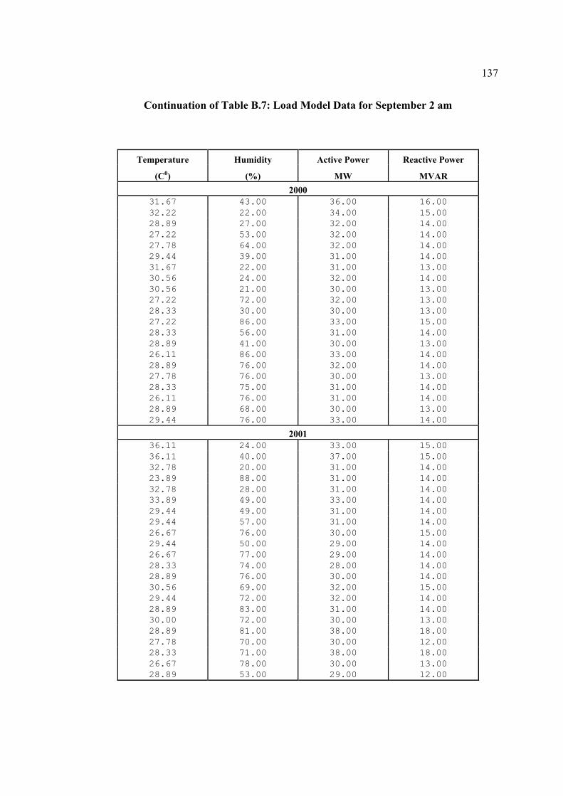
137
Continuation of Table B.7: Load Model Data for September 2 am
Temperature Humidity Active Power Reactive Power
(C0) (%) MW MVAR 2000
31.67 43.00 36.00 16.00 32.22 22.00 34.00 15.00 28.89 27.00 32.00 14.00 27.22 53.00 32.00 14.00 27.78 64.00 32.00 14.00 29.44 39.00 31.00 14.00 31.67 22.00 31.00 13.00 30.56 24.00 32.00 14.00 30.56 21.00 30.00 13.00 27.22 72.00 32.00 13.00 28.33 30.00 30.00 13.00 27.22 86.00 33.00 15.00 28.33 56.00 31.00 14.00 28.89 41.00 30.00 13.00 26.11 86.00 33.00 14.00 28.89 76.00 32.00 14.00 27.78 76.00 30.00 13.00 28.33 75.00 31.00 14.00 26.11 76.00 31.00 14.00 28.89 68.00 30.00 13.00 29.44 76.00 33.00 14.00
2001 36.11 24.00 33.00 15.00 36.11 40.00 37.00 15.00 32.78 20.00 31.00 14.00 23.89 88.00 31.00 14.00 32.78 28.00 31.00 14.00 33.89 49.00 33.00 14.00 29.44 49.00 31.00 14.00 29.44 57.00 31.00 14.00 26.67 76.00 30.00 15.00 29.44 50.00 29.00 14.00 26.67 77.00 29.00 14.00 28.33 74.00 28.00 14.00 28.89 76.00 30.00 14.00 30.56 69.00 32.00 15.00 29.44 72.00 32.00 14.00 28.89 83.00 31.00 14.00 30.00 72.00 30.00 13.00 28.89 81.00 38.00 18.00 27.78 70.00 30.00 12.00 28.33 71.00 38.00 18.00 26.67 78.00 30.00 13.00 28.89 53.00 29.00 12.00
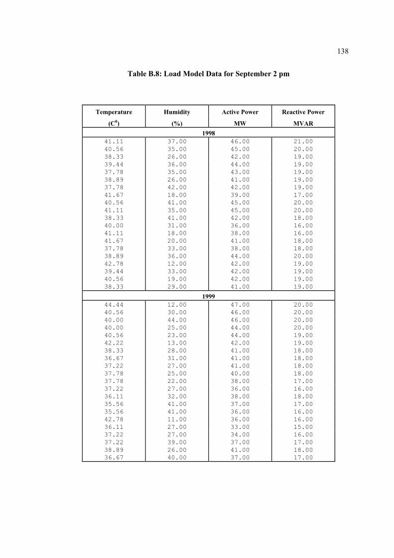
138
Table B.8: Load Model Data for September 2 pm
Temperature Humidity Active Power Reactive Power
(C0) (%) MW MVAR 1998
41.11 37.00 46.00 21.00 40.56 35.00 45.00 20.00 38.33 26.00 42.00 19.00 39.44 36.00 44.00 19.00 37.78 35.00 43.00 19.00 38.89 26.00 41.00 19.00 37.78 42.00 42.00 19.00 41.67 18.00 39.00 17.00 40.56 41.00 45.00 20.00 41.11 35.00 45.00 20.00 38.33 41.00 42.00 18.00 40.00 31.00 36.00 16.00 41.11 18.00 38.00 16.00 41.67 20.00 41.00 18.00 37.78 33.00 38.00 18.00 38.89 36.00 44.00 20.00 42.78 12.00 42.00 19.00 39.44 33.00 42.00 19.00 40.56 19.00 42.00 19.00 38.33 29.00 41.00 19.00
1999 44.44 12.00 47.00 20.00 40.56 30.00 46.00 20.00 40.00 44.00 46.00 20.00 40.00 25.00 44.00 20.00 40.56 23.00 44.00 19.00 42.22 13.00 42.00 19.00 38.33 28.00 41.00 18.00 36.67 31.00 41.00 18.00 37.22 27.00 41.00 18.00 37.78 25.00 40.00 18.00 37.78 22.00 38.00 17.00 37.22 27.00 36.00 16.00 36.11 32.00 38.00 18.00 35.56 41.00 37.00 17.00 35.56 41.00 36.00 16.00 42.78 11.00 36.00 16.00 36.11 27.00 33.00 15.00 37.22 27.00 34.00 16.00 37.22 39.00 37.00 17.00 38.89 26.00 41.00 18.00 36.67 40.00 37.00 17.00

139
Continuation of Table B.8: Load Model Data for September 2 pm
Temperature Humidity Active Power Reactive Power
(C0) (%) MW MVAR 2000
38.33 12.00 39.00 17.00 36.11 28.00 40.00 17.00 38.89 16.00 38.00 17.00 37.22 33.00 39.00 18.00 37.22 22.00 36.00 16.00 37.22 26.00 38.00 16.00 40.00 13.00 38.00 16.00 37.78 24.00 37.00 16.00 38.89 17.00 37.00 16.00 38.33 20.00 38.00 17.00 38.33 19.00 37.00 16.00 38.89 22.00 39.00 17.00 40.00 10.00 38.00 16.00 40.56 9.00 36.00 16.00 36.11 35.00 38.00 17.00 35.56 44.00 38.00 16.00 39.44 12.00 35.00 15.00 36.67 32.00 36.00 16.00 39.44 20.00 35.00 16.00 37.78 19.00 36.00 16.00 37.22 30.00 38.00 17.00
2001 40.00 29.00 41.00 17.00 40.56 15.00 38.00 17.00 40.00 17.00 37.00 17.00 41.67 12.00 37.00 17.00 43.89 9.00 38.00 16.00 39.44 24.00 38.00 16.00 38.33 18.00 37.00 18.00 37.78 29.00 36.00 16.00 36.67 30.00 36.00 18.00 37.78 27.00 37.00 17.00 35.00 48.00 35.00 16.00 34.44 42.00 34.00 17.00 37.22 39.00 35.00 17.00 37.22 33.00 37.00 18.00 40.00 10.00 36.00 16.00 40.00 18.00 38.00 17.00 41.11 11.00 38.00 18.00 41.67 9.00 36.00 15.00 40.00 19.00 38.00 18.00 40.00 20.00 36.00 14.00 38.89 26.00 34.00 16.00 41.11 18.00 35.00 15.00

140
Appendix C
ERROR BARS PLOTS

141
Figure C.1: Error Bar for the Active Power Model for 1998 June at 2 am
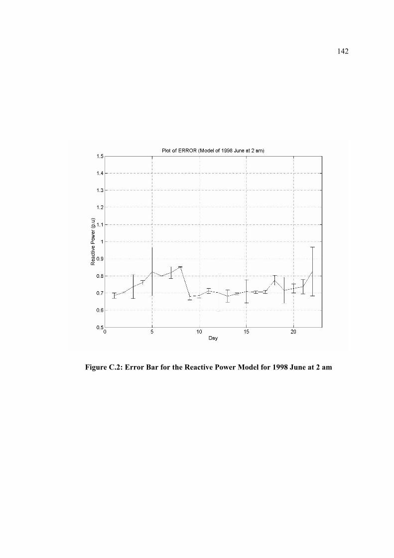
142
Figure C.2: Error Bar for the Reactive Power Model for 1998 June at 2 am
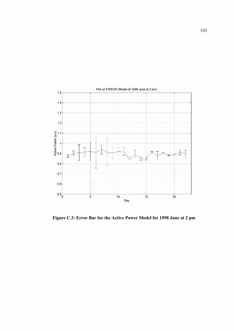
143
Figure C.3: Error Bar for the Active Power Model for 1998 June at 2 pm
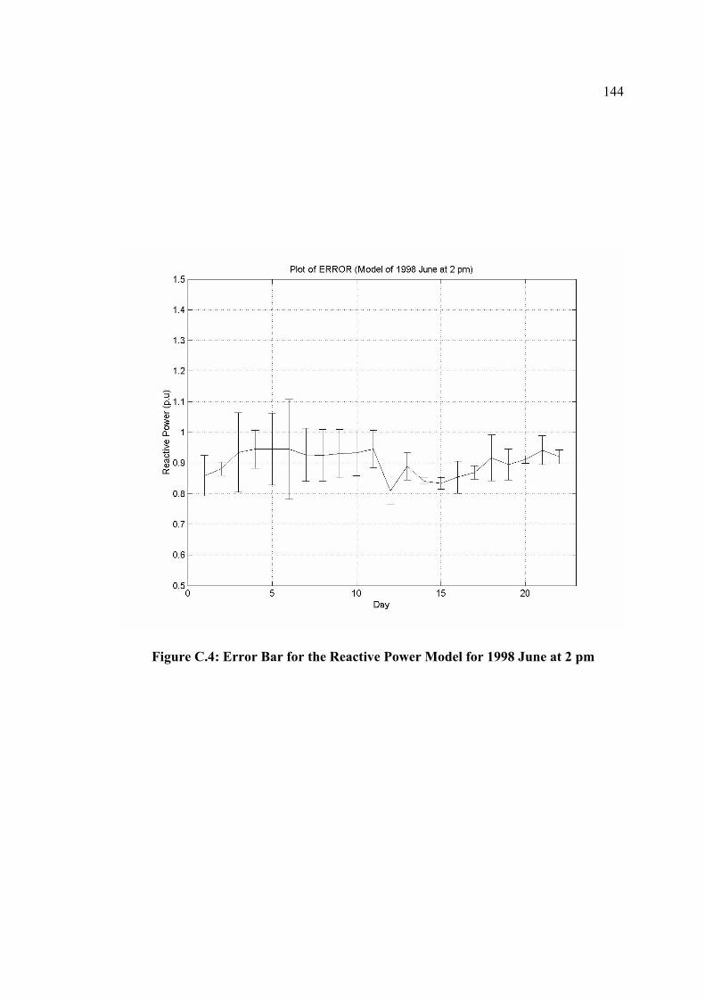
144
Figure C.4: Error Bar for the Reactive Power Model for 1998 June at 2 pm
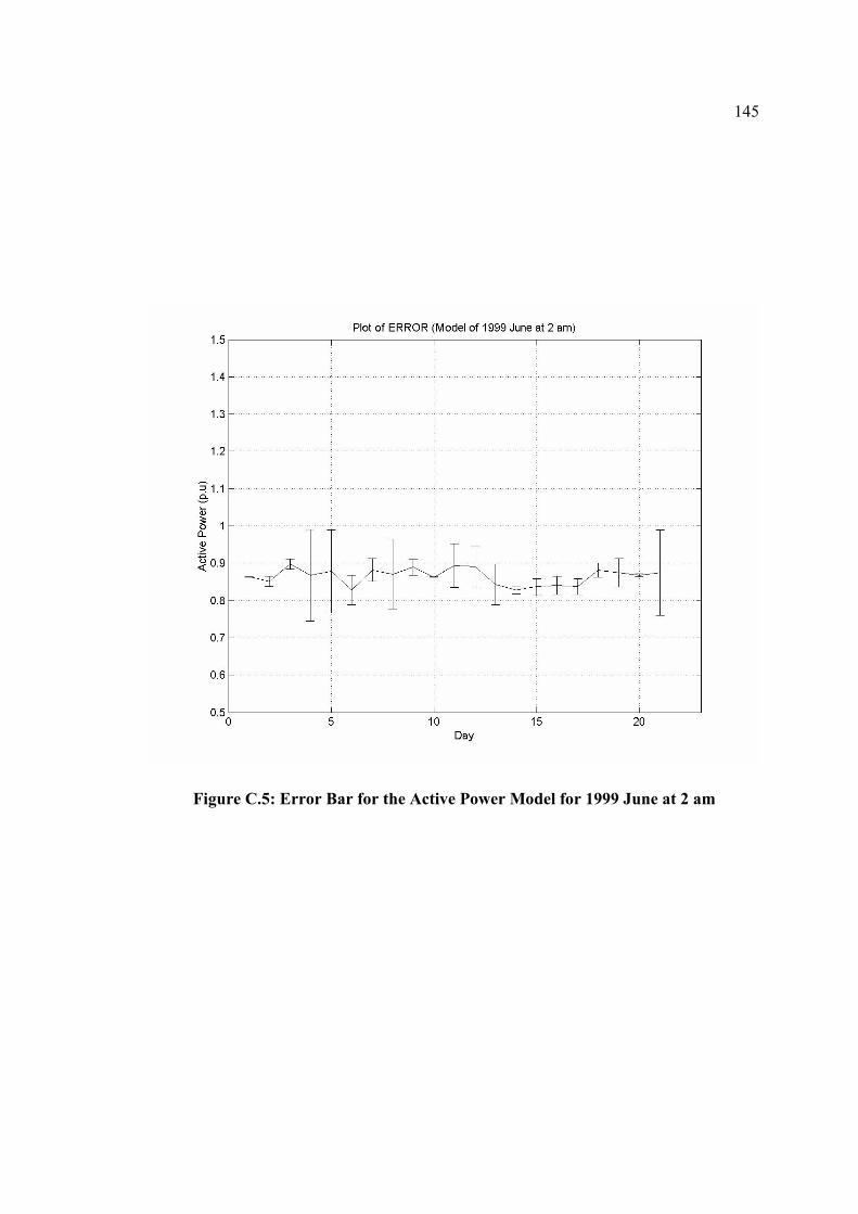
145
Figure C.5: Error Bar for the Active Power Model for 1999 June at 2 am
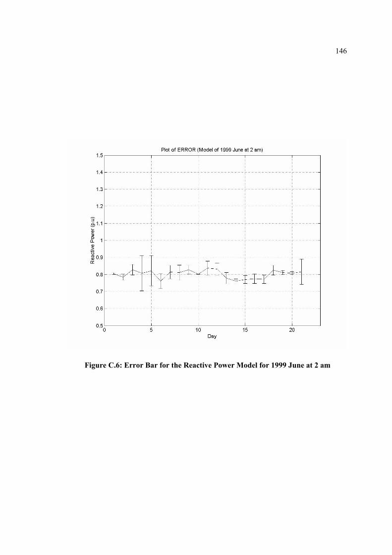
146
Figure C.6: Error Bar for the Reactive Power Model for 1999 June at 2 am
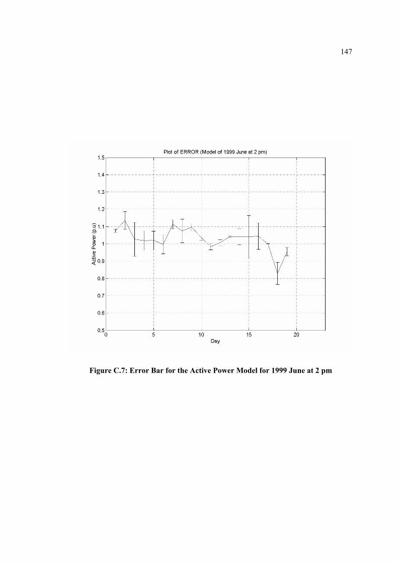
147
Figure C.7: Error Bar for the Active Power Model for 1999 June at 2 pm
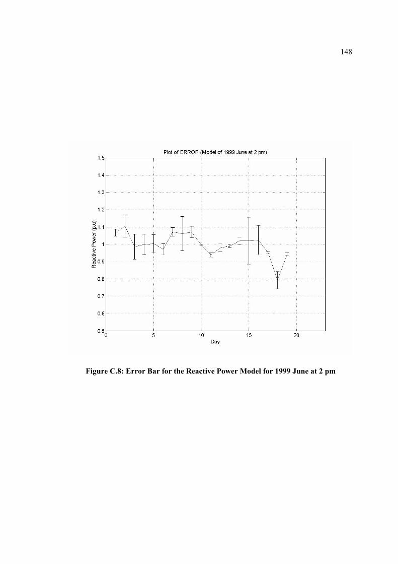
148
Figure C.8: Error Bar for the Reactive Power Model for 1999 June at 2 pm
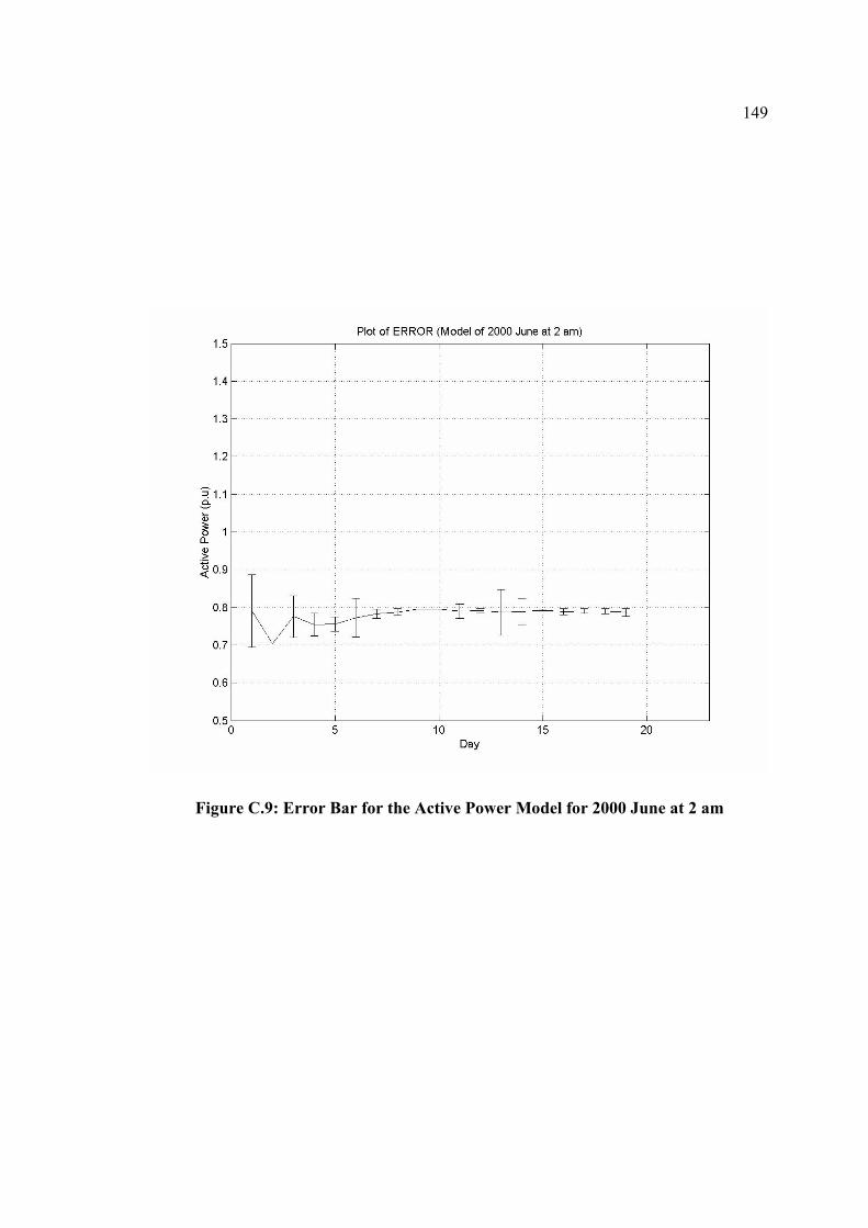
149
Figure C.9: Error Bar for the Active Power Model for 2000 June at 2 am
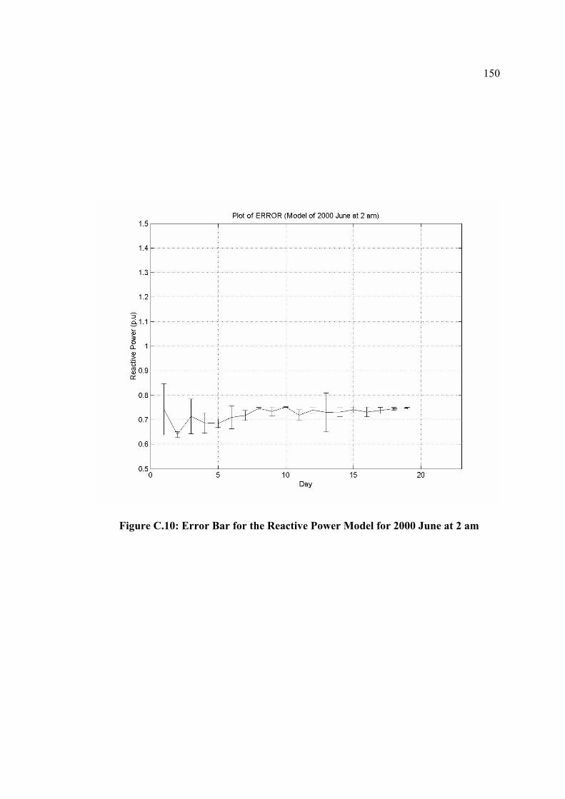
150
Figure C.10: Error Bar for the Reactive Power Model for 2000 June at 2 am
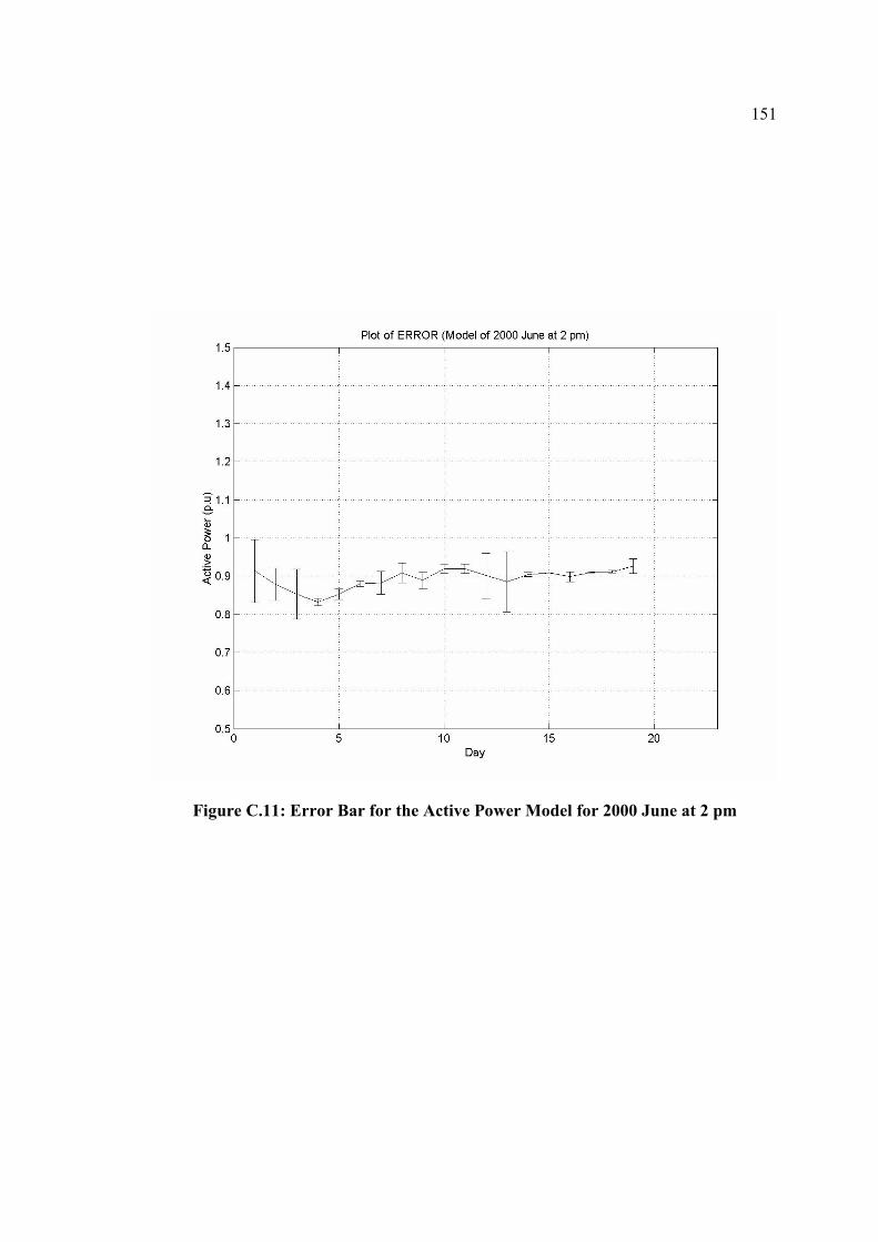
151
Figure C.11: Error Bar for the Active Power Model for 2000 June at 2 pm
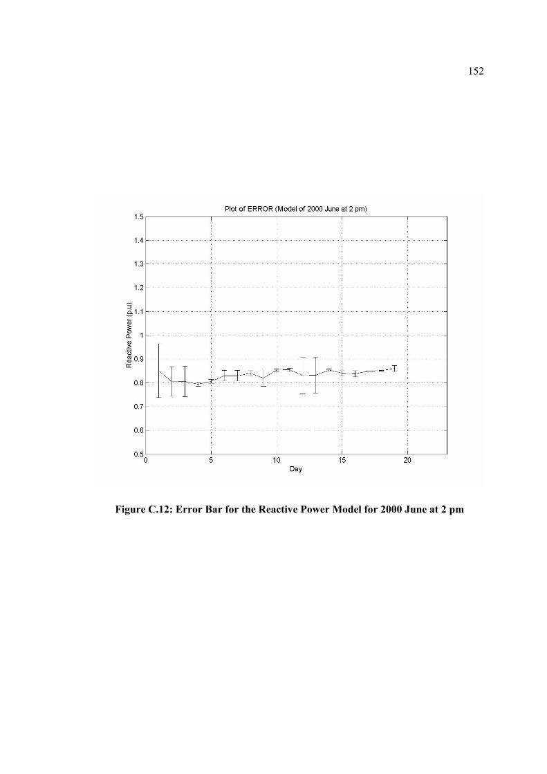
152
Figure C.12: Error Bar for the Reactive Power Model for 2000 June at 2 pm
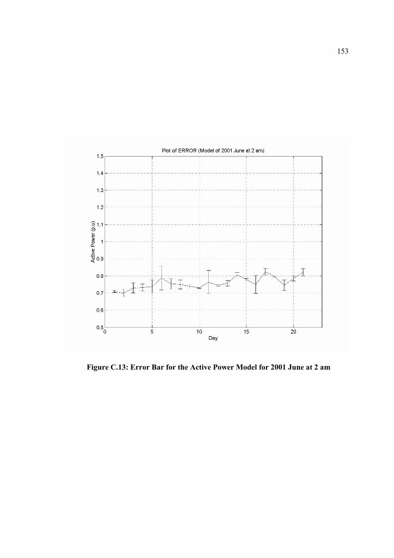
153
Figure C.13: Error Bar for the Active Power Model for 2001 June at 2 am
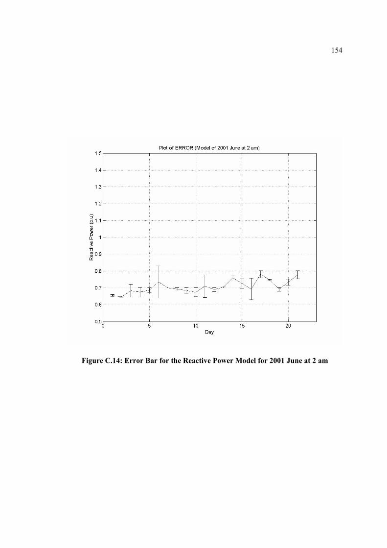
154
Figure C.14: Error Bar for the Reactive Power Model for 2001 June at 2 am

155
Figure C.15: Error Bar for the Active Power Model for 2001 June at 2 pm
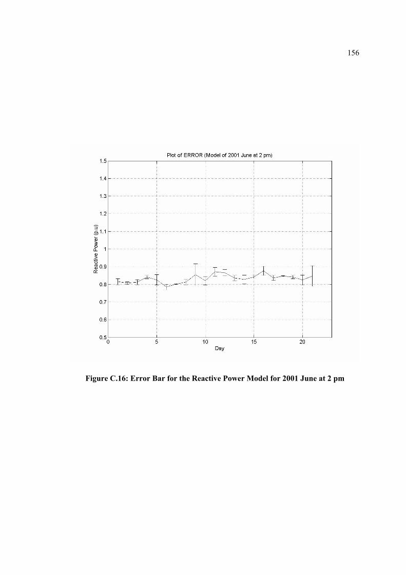
156
Figure C.16: Error Bar for the Reactive Power Model for 2001 June at 2 pm

157
Figure C.17: Error Bar for the Active Power Model for 1998 July at 2 am
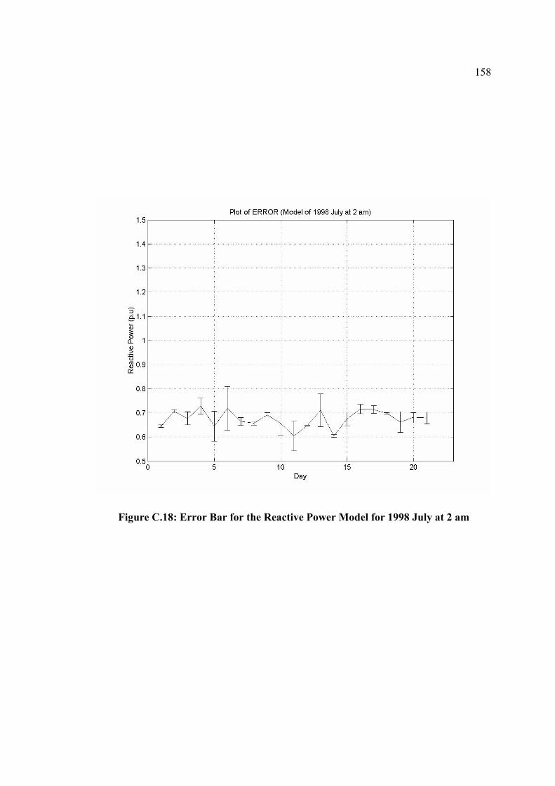
158
Figure C.18: Error Bar for the Reactive Power Model for 1998 July at 2 am
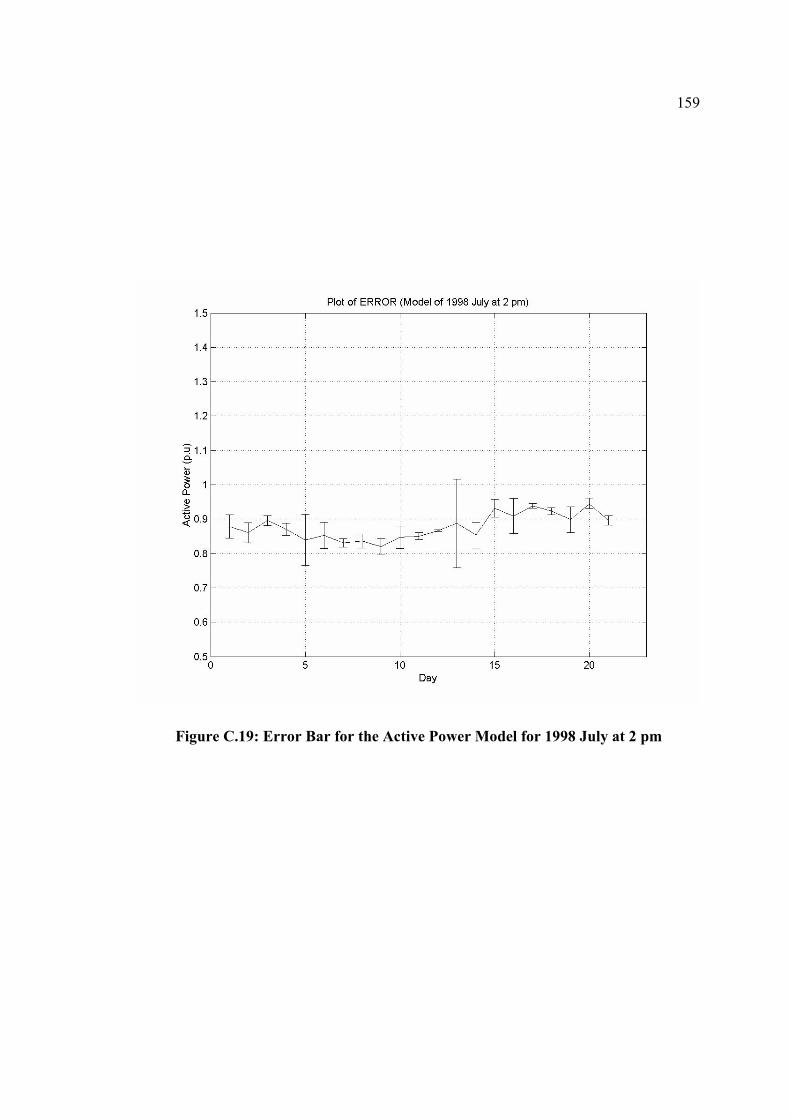
159
Figure C.19: Error Bar for the Active Power Model for 1998 July at 2 pm
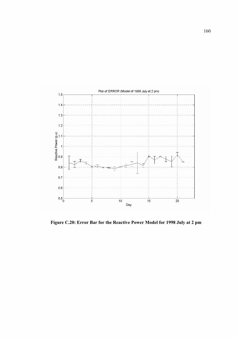
160
Figure C.20: Error Bar for the Reactive Power Model for 1998 July at 2 pm
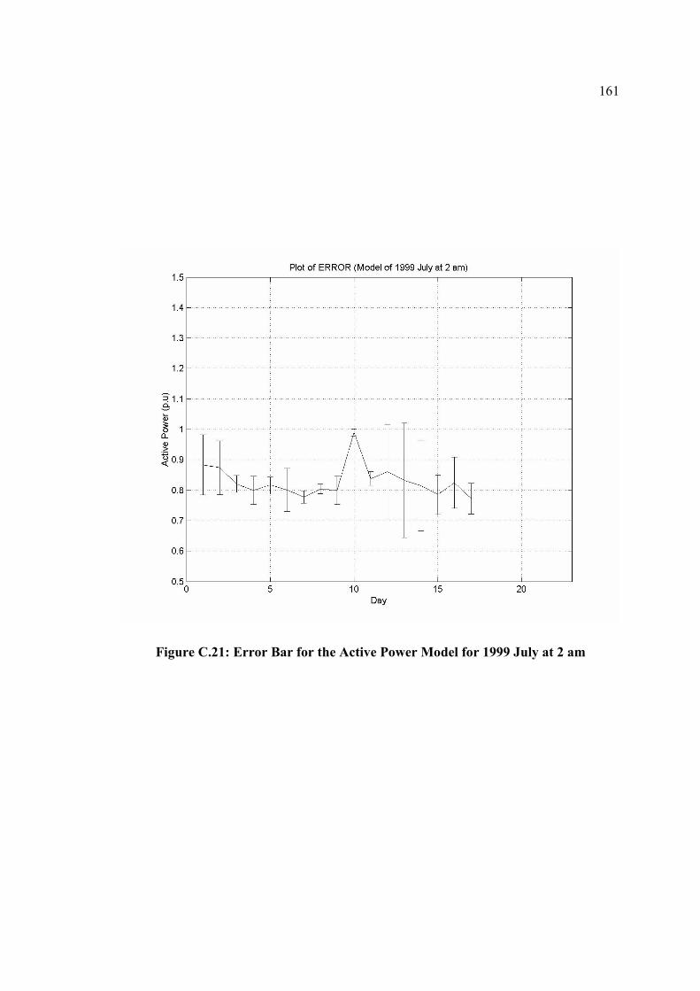
161
Figure C.21: Error Bar for the Active Power Model for 1999 July at 2 am
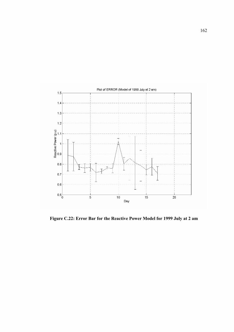
162
Figure C.22: Error Bar for the Reactive Power Model for 1999 July at 2 am

163
Figure C.23: Error Bar for the Active Power Model for 1999 July at 2 pm
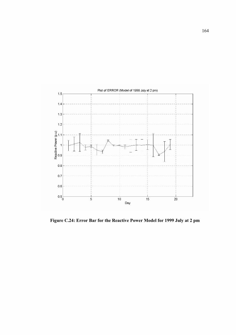
164
Figure C.24: Error Bar for the Reactive Power Model for 1999 July at 2 pm
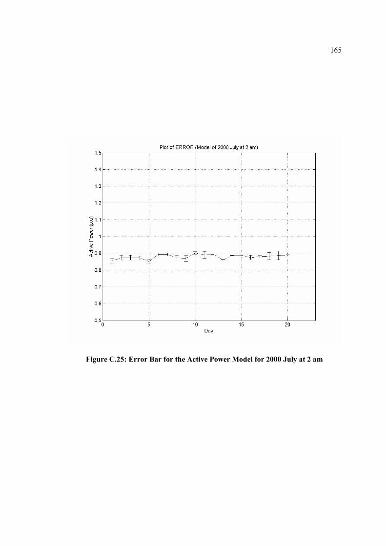
165
Figure C.25: Error Bar for the Active Power Model for 2000 July at 2 am
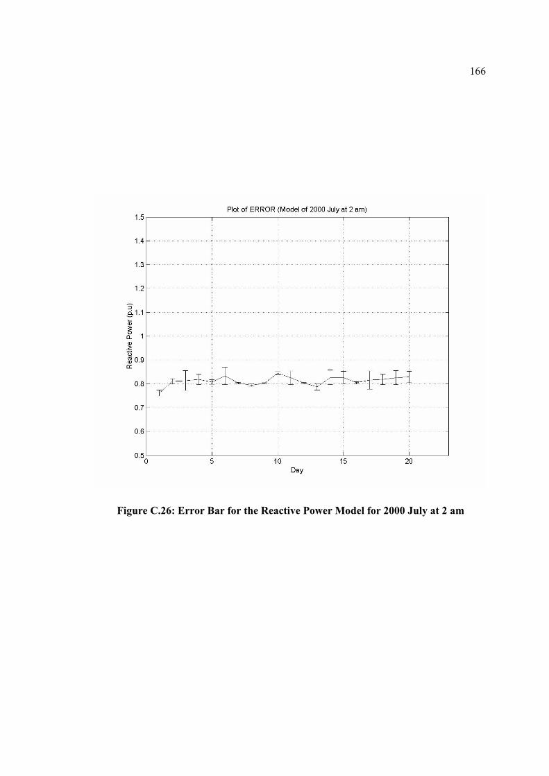
166
Figure C.26: Error Bar for the Reactive Power Model for 2000 July at 2 am
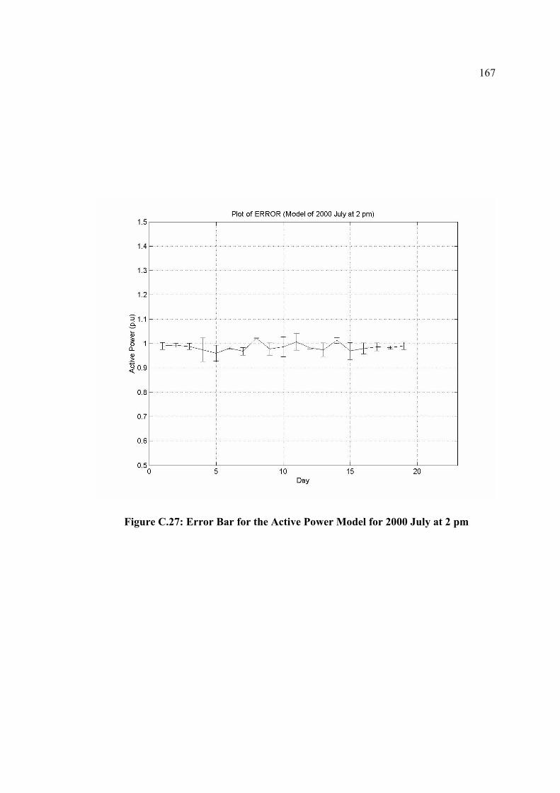
167
Figure C.27: Error Bar for the Active Power Model for 2000 July at 2 pm
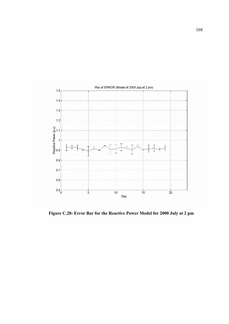
168
Figure C.28: Error Bar for the Reactive Power Model for 2000 July at 2 pm
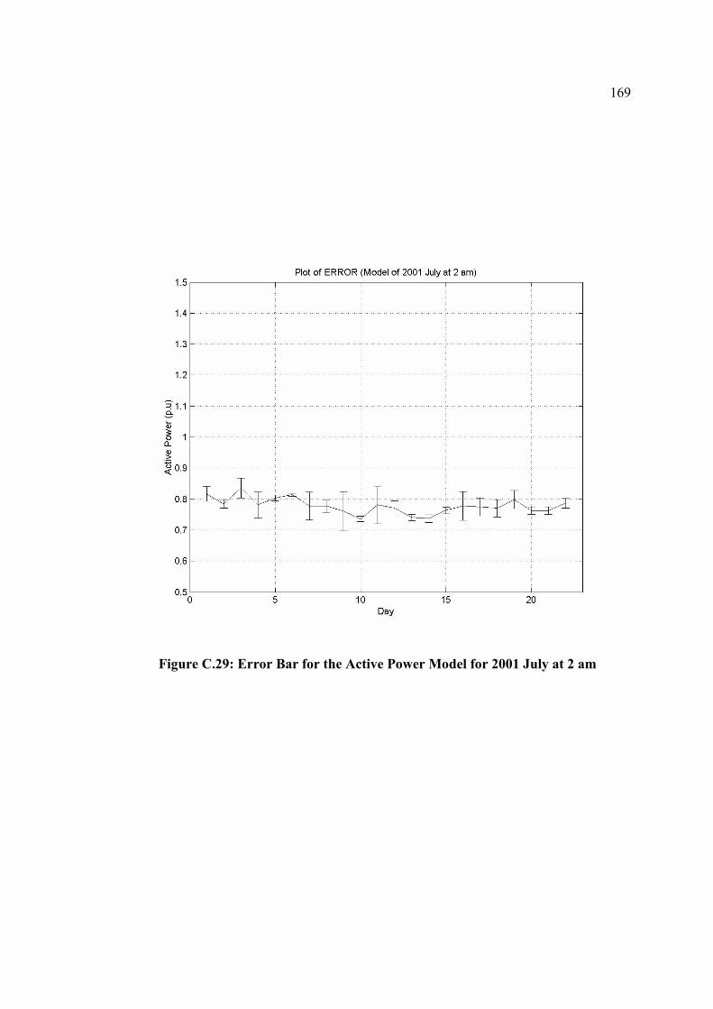
169
Figure C.29: Error Bar for the Active Power Model for 2001 July at 2 am
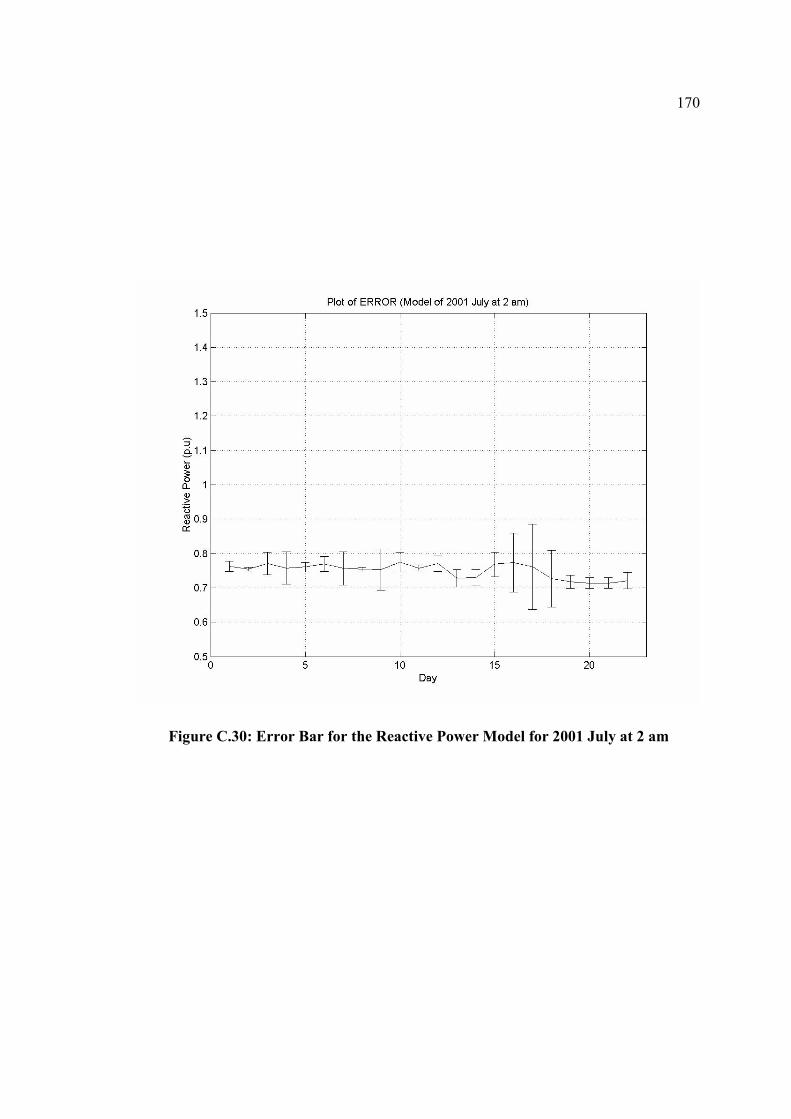
170
Figure C.30: Error Bar for the Reactive Power Model for 2001 July at 2 am
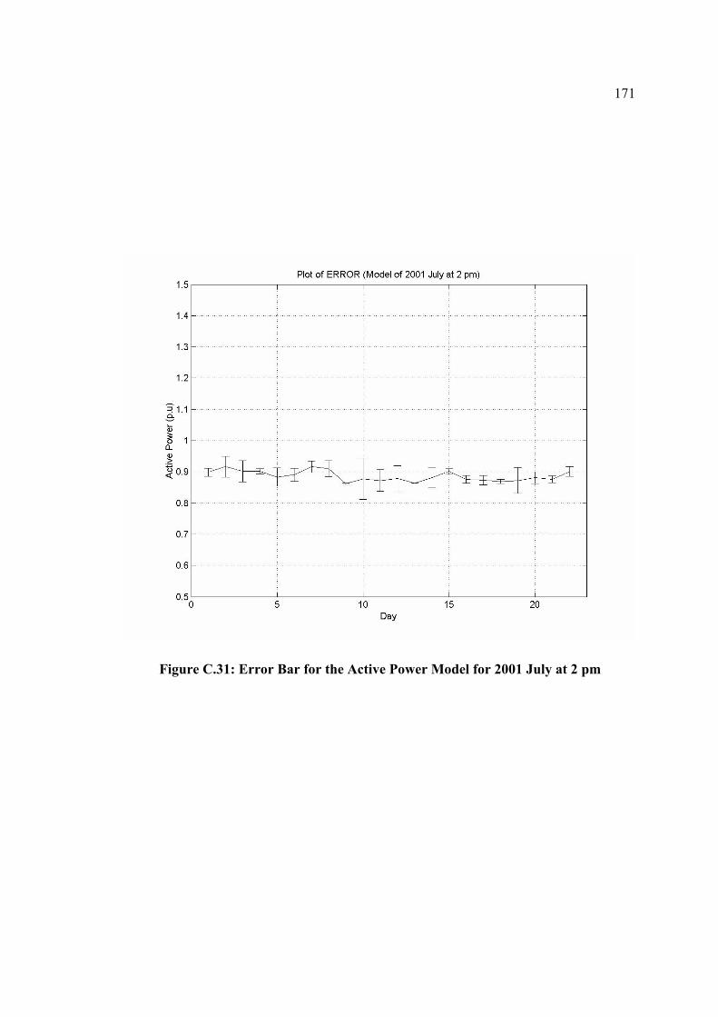
171
Figure C.31: Error Bar for the Active Power Model for 2001 July at 2 pm
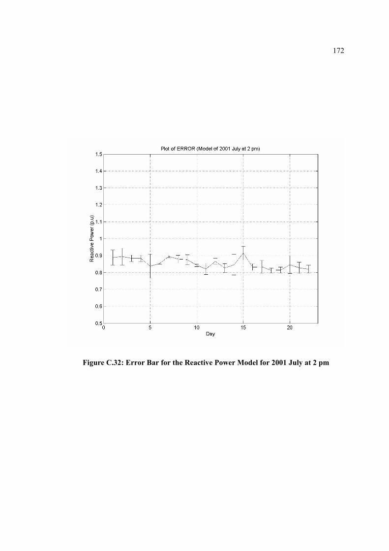
172
Figure C.32: Error Bar for the Reactive Power Model for 2001 July at 2 pm
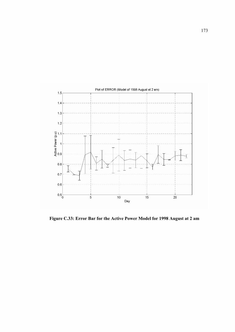
173
Figure C.33: Error Bar for the Active Power Model for 1998 August at 2 am
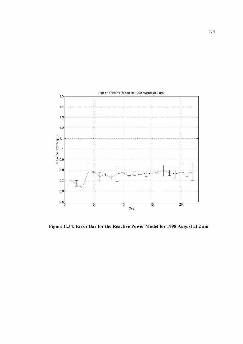
174
Figure C.34: Error Bar for the Reactive Power Model for 1998 August at 2 am
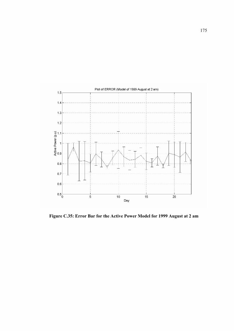
175
Figure C.35: Error Bar for the Active Power Model for 1999 August at 2 am
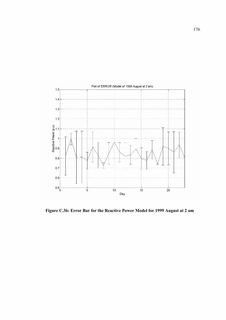
176
Figure C.36: Error Bar for the Reactive Power Model for 1999 August at 2 am
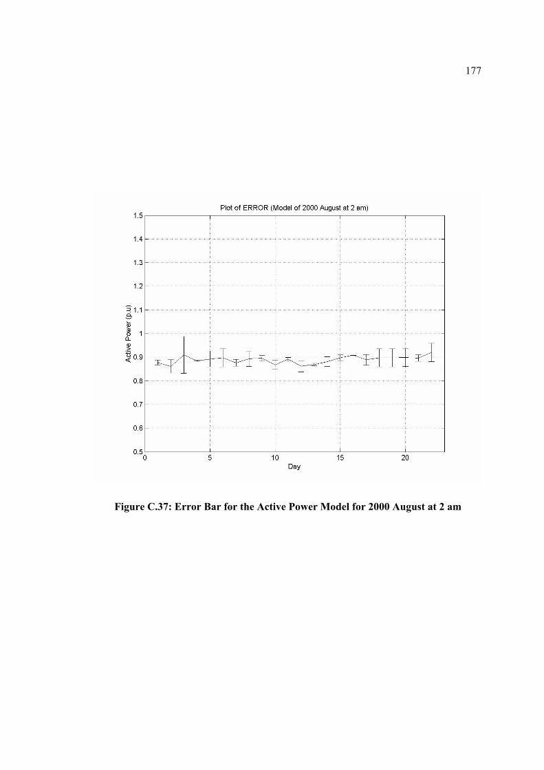
177
Figure C.37: Error Bar for the Active Power Model for 2000 August at 2 am
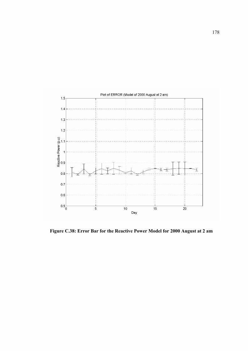
178
Figure C.38: Error Bar for the Reactive Power Model for 2000 August at 2 am
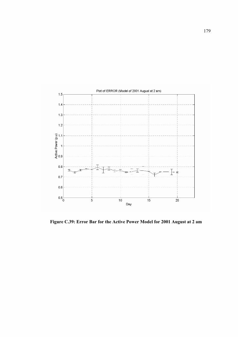
179
Figure C.39: Error Bar for the Active Power Model for 2001 August at 2 am
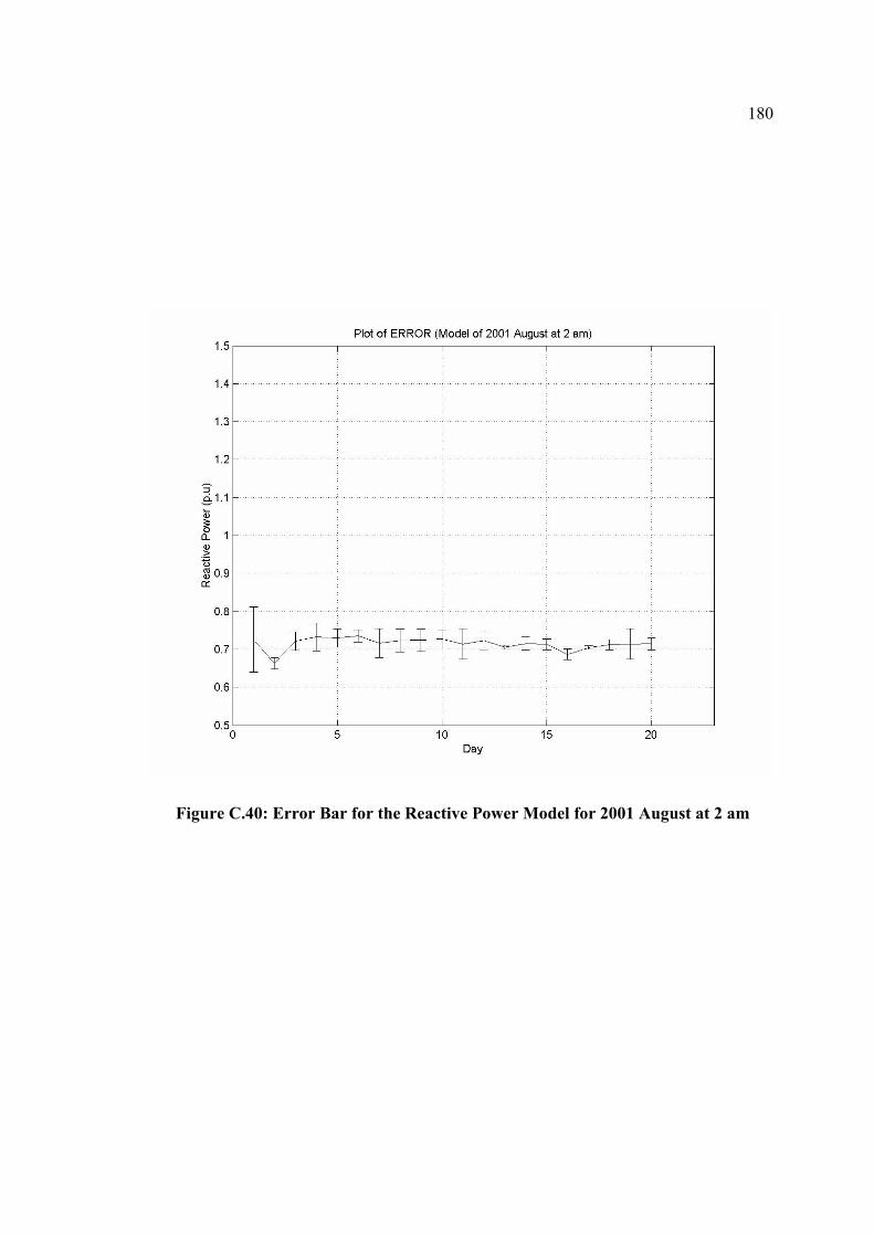
180
Figure C.40: Error Bar for the Reactive Power Model for 2001 August at 2 am
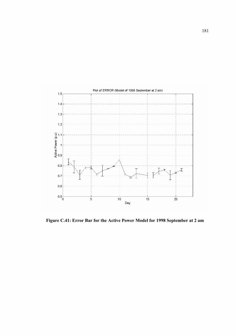
181
Figure C.41: Error Bar for the Active Power Model for 1998 September at 2 am

182
Figure C.42: Error Bar for the Reactive Power Model for 1998 September at 2 am
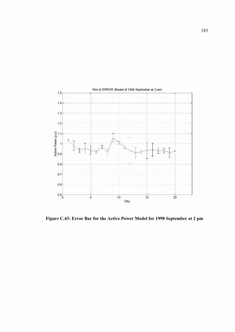
183
Figure C.43: Error Bar for the Active Power Model for 1998 September at 2 pm
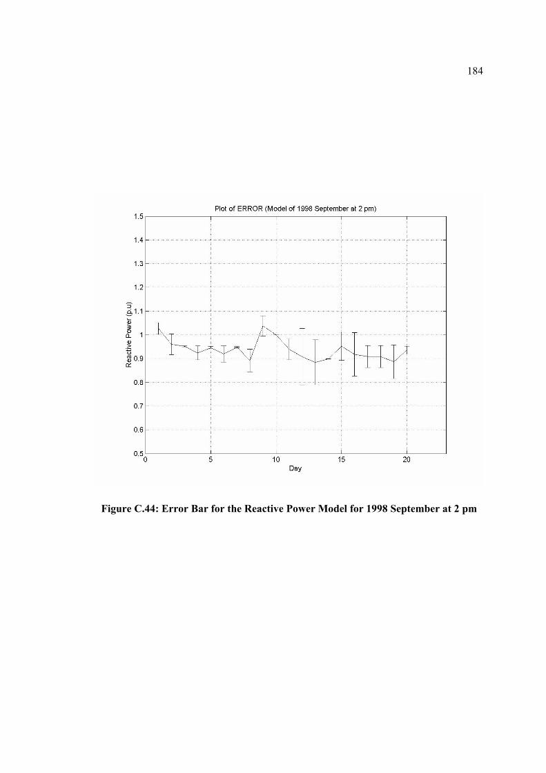
184
Figure C.44: Error Bar for the Reactive Power Model for 1998 September at 2 pm
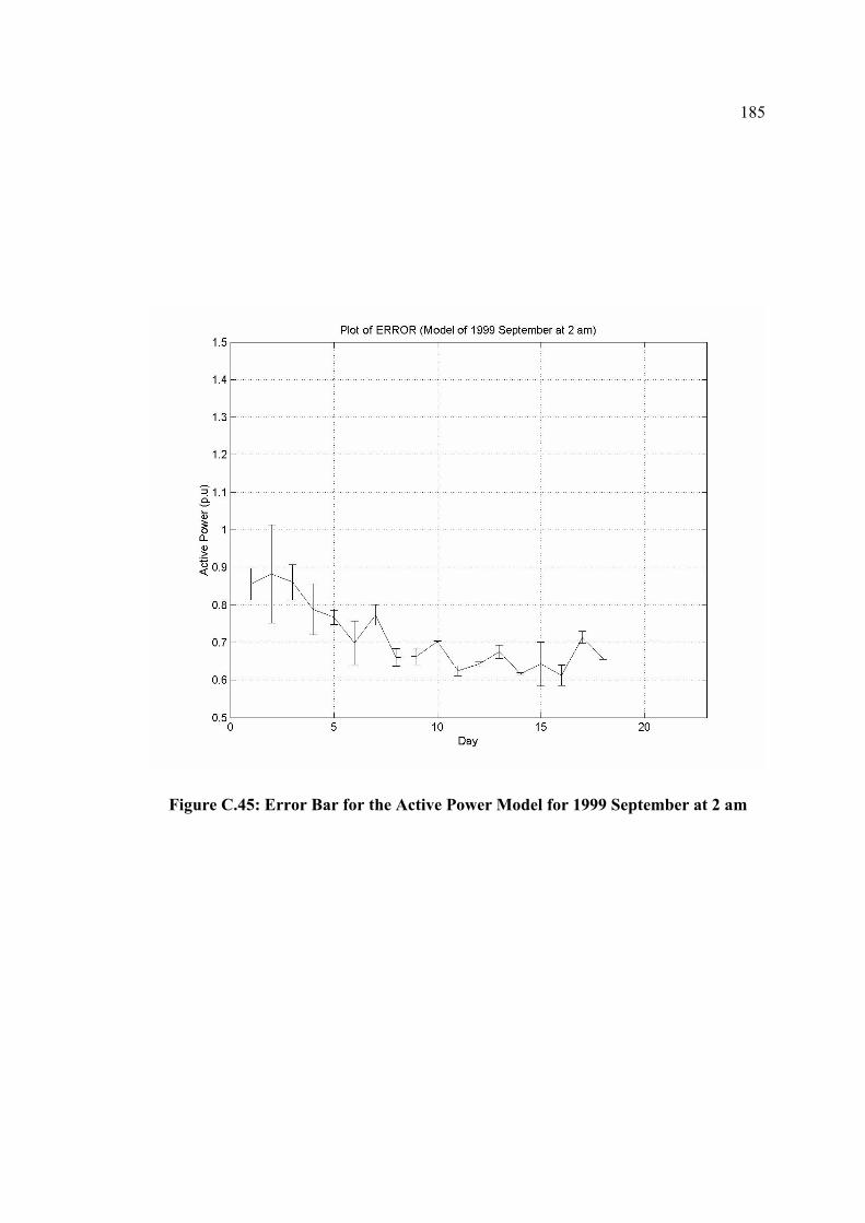
185
Figure C.45: Error Bar for the Active Power Model for 1999 September at 2 am
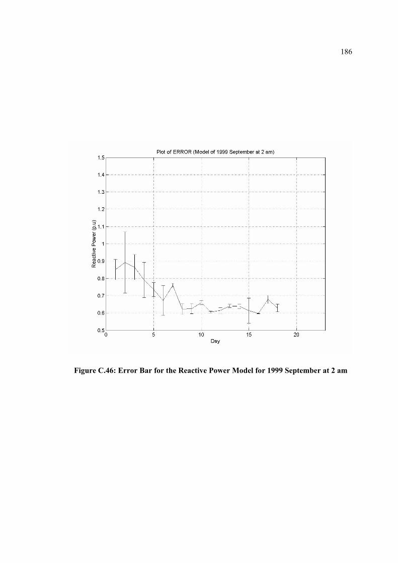
186
Figure C.46: Error Bar for the Reactive Power Model for 1999 September at 2 am
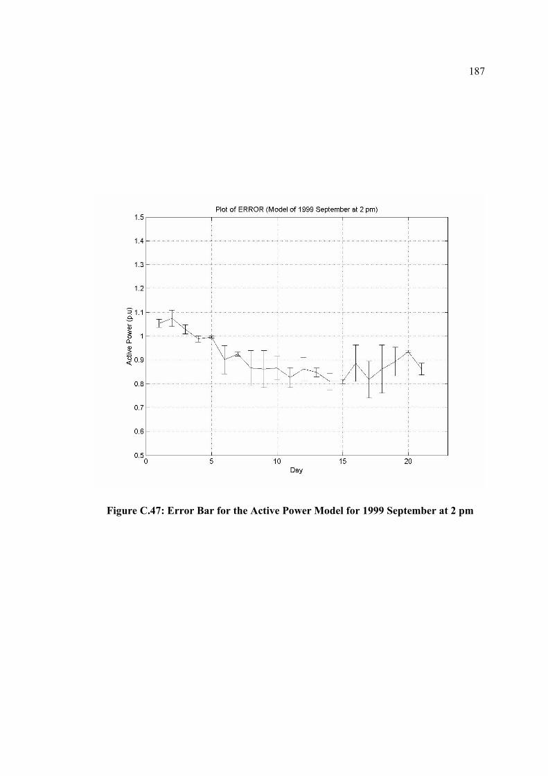
187
Figure C.47: Error Bar for the Active Power Model for 1999 September at 2 pm
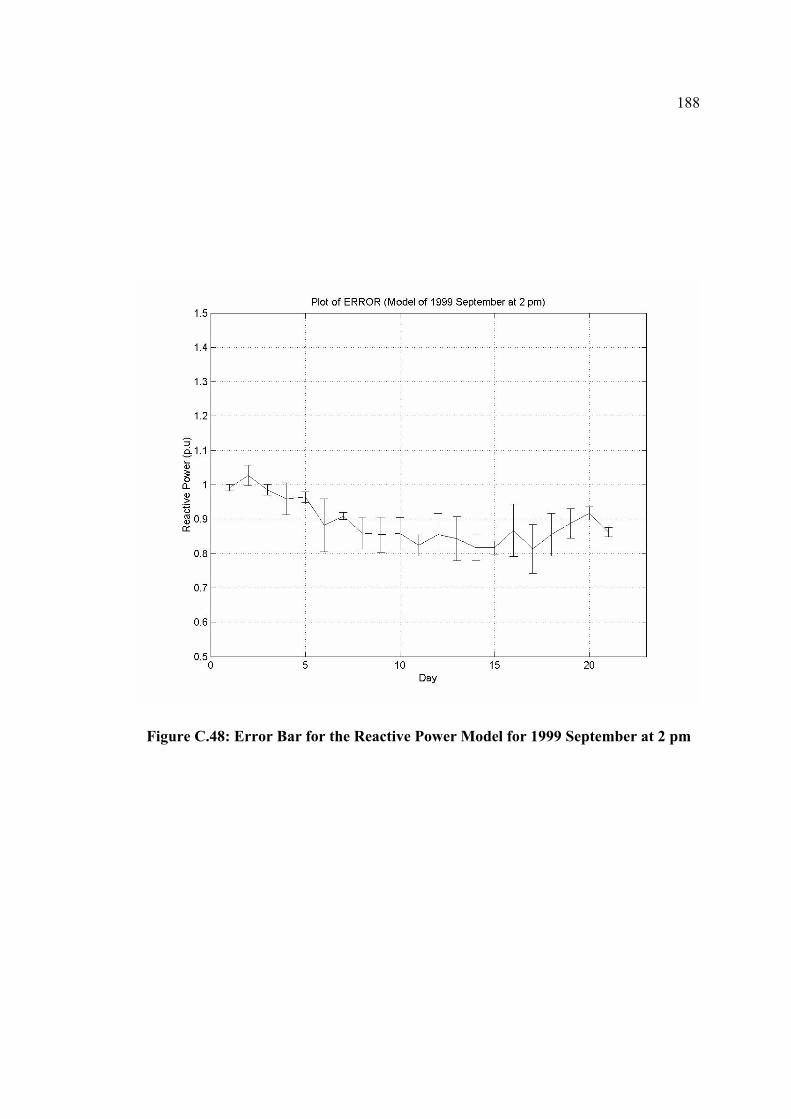
188
Figure C.48: Error Bar for the Reactive Power Model for 1999 September at 2 pm
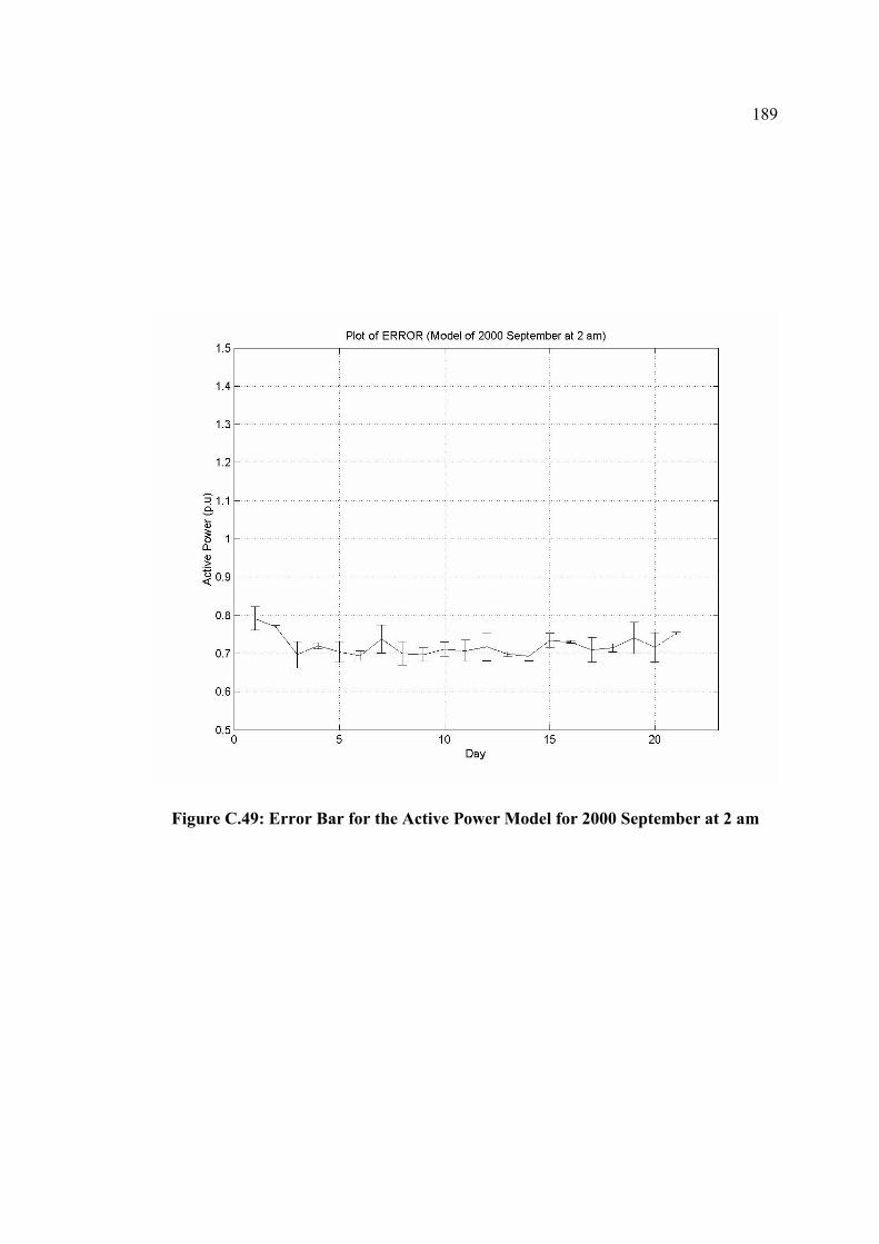
189
Figure C.49: Error Bar for the Active Power Model for 2000 September at 2 am
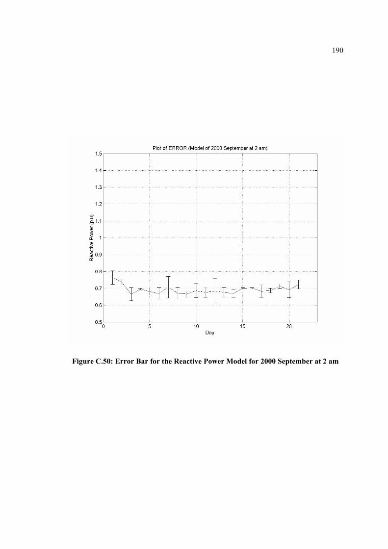
190
Figure C.50: Error Bar for the Reactive Power Model for 2000 September at 2 am

191
Figure C.51: Error Bar for the Active Power Model for 2000 September at 2 pm
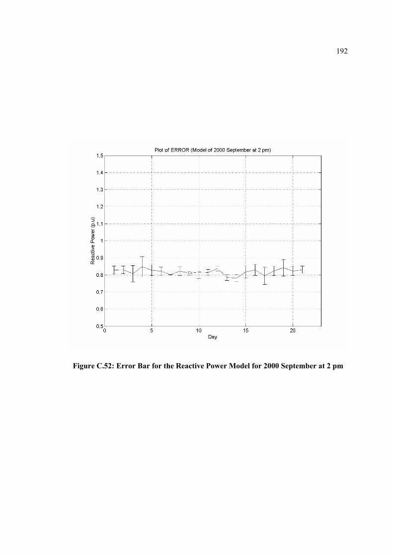
192
Figure C.52: Error Bar for the Reactive Power Model for 2000 September at 2 pm
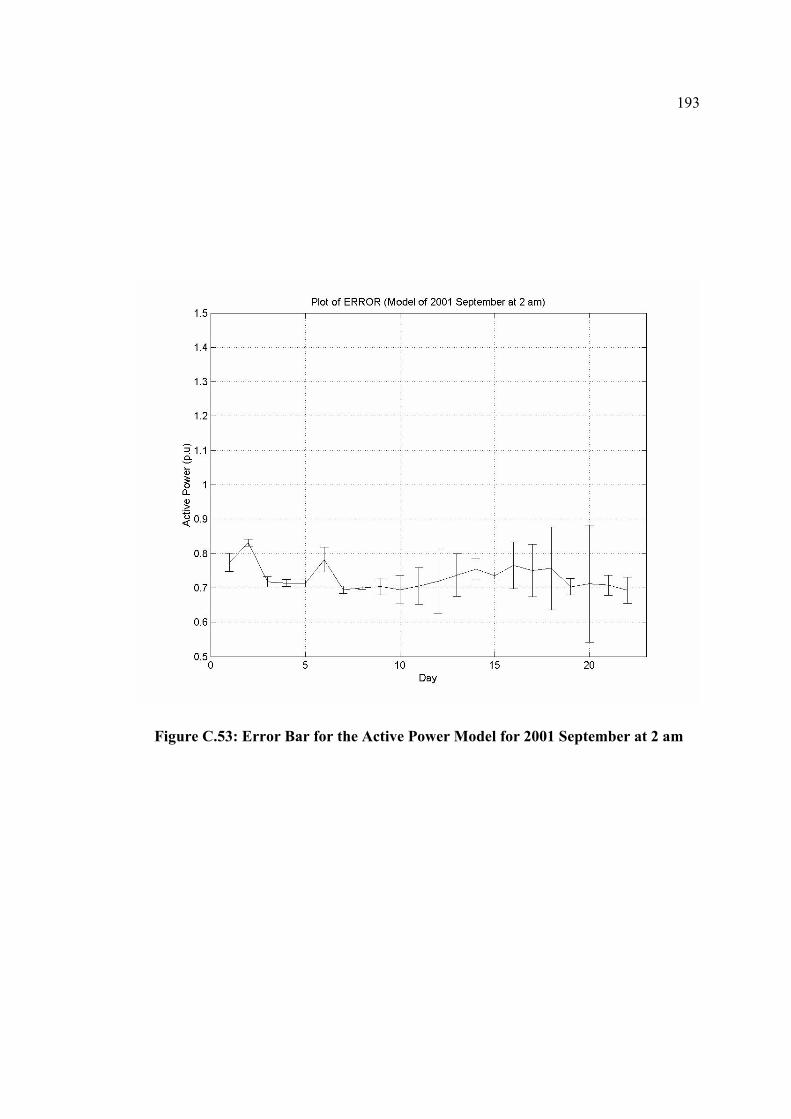
193
Figure C.53: Error Bar for the Active Power Model for 2001 September at 2 am
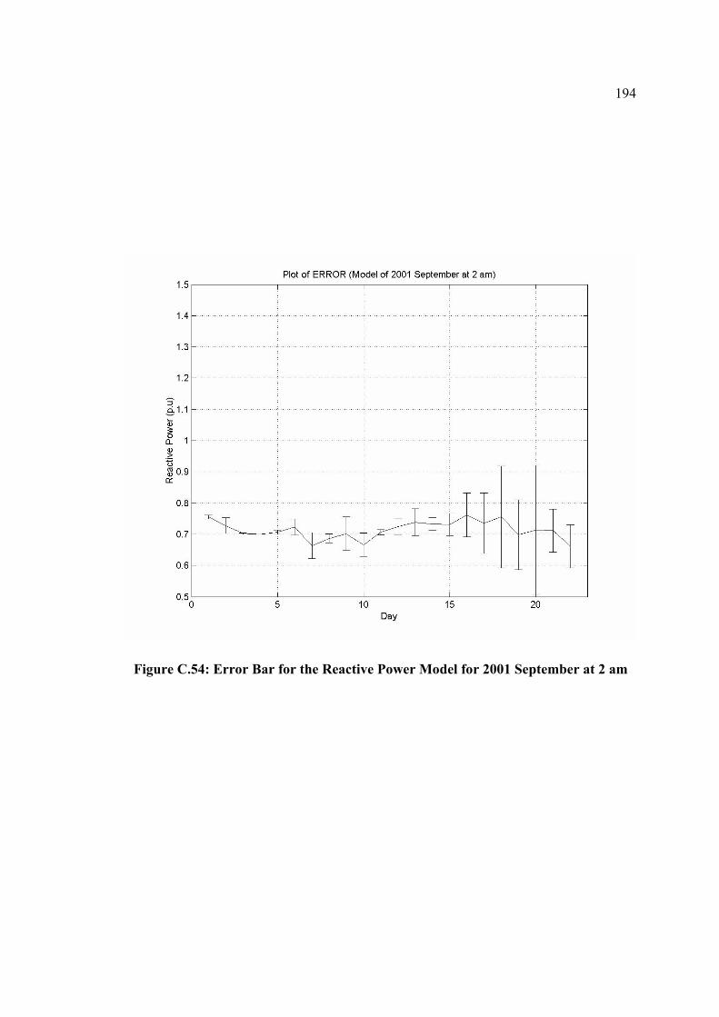
194
Figure C.54: Error Bar for the Reactive Power Model for 2001 September at 2 am
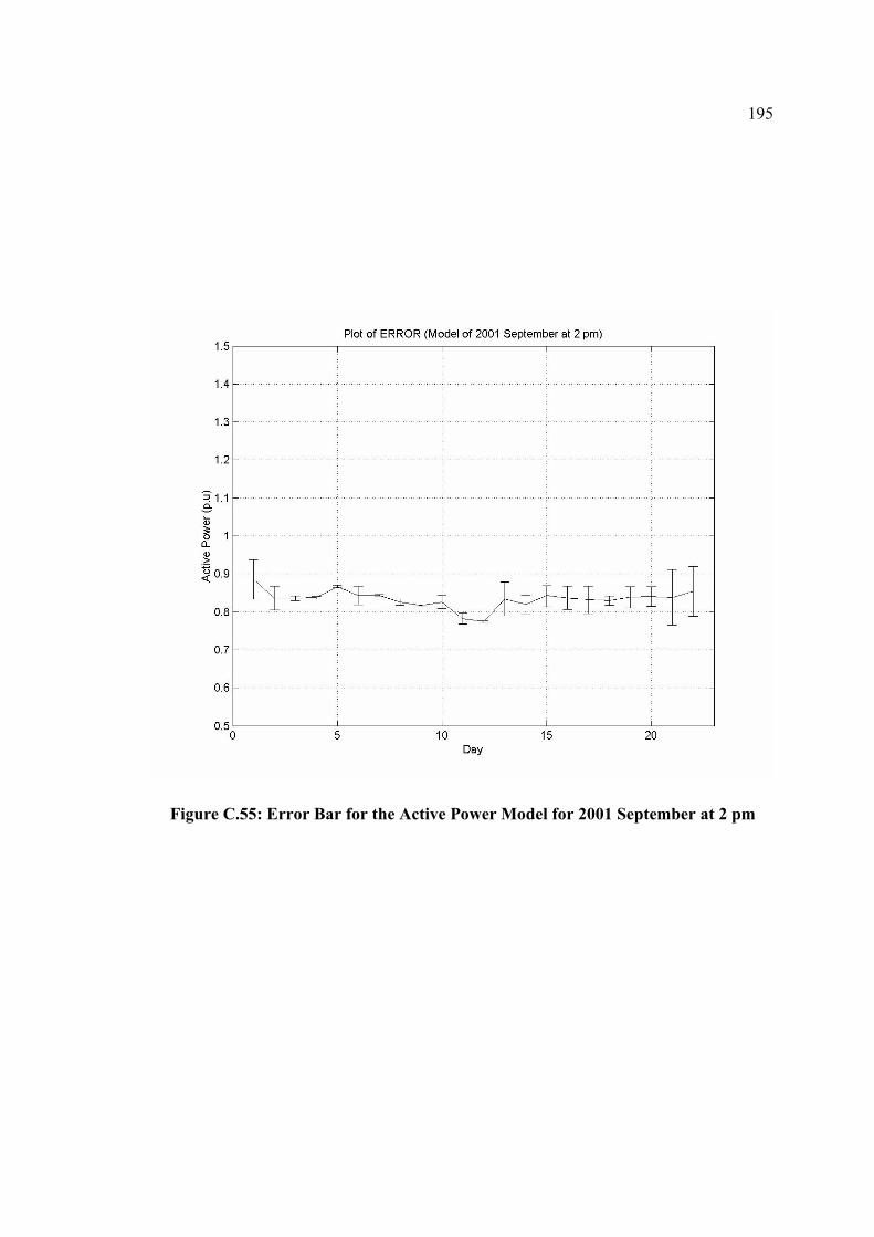
195
Figure C.55: Error Bar for the Active Power Model for 2001 September at 2 pm
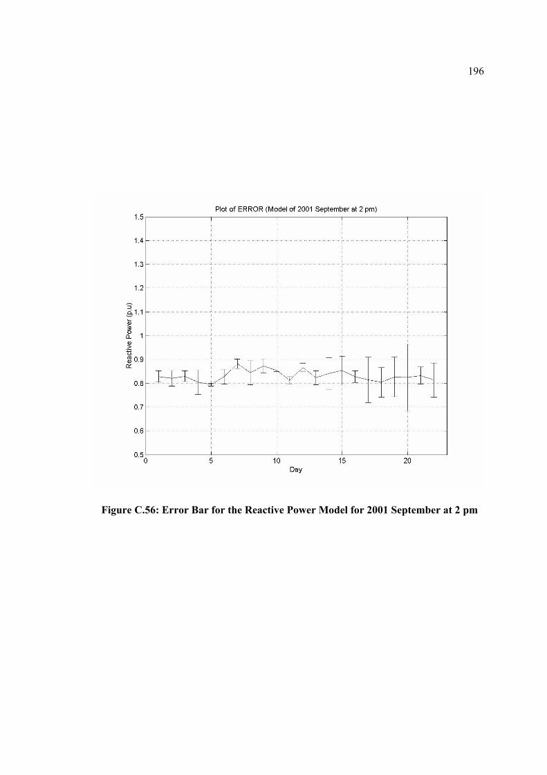
196
Figure C.56: Error Bar for the Reactive Power Model for 2001 September at 2 pm

197
Bibliography
[1]. Price, W.W.; K.A. Wirgau; etc, ”Load Modeling for Power Flow and Transient
Stability Computer Studies,” IEEE Trans. Vol.3, No. 1, pp. 180-187, Feb. 1988.
[2]. Hajagos, L.; B. Danai, “Laboratory Measurements And Models Of Modern Loads
And Their Effect On Voltage Stability Studies,” IEEE Trans. Vol. 13, No. 2, pp.
584-591, May 1998.
[3]. IEEE Task Force, “Load Representation for Dynamic Performance Analysis,” IEEE
Trans. Vol. 8, No. 2, pp. 472-481, May 1993.
[4]. Coker, M.; H. Kgasoane, “Load Modeling,” pp. 663-668, IEEE 1999.
[5]. T. Siyambalapitiya, R. Dugeno, M. Al-Mulhim, “Special Considerations In Demand
Forecasting At Electric Utilities” 2nd Regional Conference of CIGRE Arab State
Committees, May 1997.
[6]. J. Nanthakumar, A. Al-Najim, “Development Of Electricity Demand Forecasts
Based On Weather-Related Parameters” Regional Conference of CIGRE Arab State
Committees, May 1999.
198
[7]. General Electric Co., “Load Modeling for Power Flow and Transient Stability
Computer Studies,” EBRI EL-5003, Vol. 2, Project 849-7 final report, Jan. 1987.
[8]. Dias, L.G.; M.E. El-Hawary, “Nonlinear Parameter Estimation Experiments For
Static Load Modeling In Electric Power Systems,” IEE Proceedings, Vol. 136, No.
2, pp. 68-77, Mar. 1989.
[9]. Beghzouz, Y.; C. Quist, “Composite Load Model Derivation From Recorded Field
Data,” pp. 713-718, IEEE 1998.
[10]. Ohyama, T.; A. Watanabe; K. Nishimura; S. Tsuruta, “Voltage Dependence Of
Composite Loads In Power Systems,” IEEE Trans. PAS-104, No. 11, pp. 3064-
3073, Nov. 1985.
[11]. IEEE Task Force, “Bibliography on Load Models for Power Flow and Dynamic
Performance Simulation,” IEEE Trans. Vol. 10, No. 1, pp. 523-538, Feb. 1995.
[12]. Barakat, E.; M. Eissa, “Forecasting Monthly Peak Demand In Fast Growing Electric
Utility Using A Composite Multiregression-Decomposition Model,” IEEE
Proceedings, Vol. 136, No. 1, pp. 35-41, Jan. 1989.
[13]. Ju, P.; E. Handschin; D. Karlsson, “Nonlinear Dynamic Load Modeling Model And
Parameter Estimation,” IEEE Trans.Vol. 11, No. 4, pp. 1689-1697 Nov. 1996.
199
[14]. Enander, E.; A. Sjoberg; B. Melin; etc, ”The Matlab Handbook” British Library
Cataloguing in Publication Data, ISBN 0-201-877570, 1996.
[15]. Belhadj, C.; R. Mansour, "Temperature And Humidity Impact on Power System
Load Modeling," Proceedings of the IASTED International Conference, Power and
Energy Systems, pp. 77-82, February 2003.
[16]. Daniel Karlsson, ”Voltage Stability Simulations Using Detailed Models Based On
Field Measurements,” Technical Report No. 230, Department of Electrical Power
Systems, Chalmers University of Technology, Goteborg, Sweden, June 1992.
[17]. Brice, C. W.; A. Pahwa, “Modeling And System Identification Of Residential Air
Conditioning Load,” IEEE Trans. PAS-104, No. 6, pp. 1418-1425, Jun. 1985
[18]. Dias, L.G.; M. E. El-Hawary, “Effect Of Active And Reactive Power Modeling In
Optimal Load Flow Studies,” IEE Proceedings Vol. 136, No. 5, pp. 259-263, Sept.
1989.
[19]. Khodabakhchin, B.; G. Vuong, “Modeling A Mixed Residential-Commercial Load
For Simulations Involving Large Disturbances,” IEEE Trans. Vol. 12, No. 2, pp.
791-796, May 1997.

200
Vita
• Khaled Hamed Abdullah Al-Ghamdi
• Born in Al-Baha, Saudi Arabia in Rajab 1392H.
• Received Degree of Bachelor of Science in Electrical Engineering, with third
honors, from King Fahd University of Petroleum and Minerals, Dhahran, Saudi
Arabia in January 1997.
• Working in the Saudi Electricity Company-Eastern Region Branch (SEC-ERB),
Dammam, Saudi Arabia as Planning Engineer, System Planning Department.