Embed Size (px)
Citation preview
Security Enhancement throughDirect Non-Disruptive Load Control
Final Project ReportPart II
Power Systems Engineering Research Center
A National Science FoundationIndustry/University Cooperative Research Center
since 1996
PSERC
Power Systems Engineering Research Center
Security Enhancement through Direct Non-Disruptive Load Control
Final Project Report
Part II
Report Authors
Vijay Vittal, Arizona State University Badri Ramanathan, Iowa State University
PSERC Publication 06-02
January 2006

Information about this project For information about this project contact: Vijay Vittal Ira A. Fulton Chair Professor Arizona State University Department of Electrical Engineering Tempe, AZ 85287 Phone: 480-965-1879 Fax: 480-965-0745 Email: [email protected] Power Systems Engineering Research Center This is a project report from the Power Systems Engineering Research Center (PSERC). PSERC is a multi-university Center conducting research on challenges facing a restructuring electric power industry and educating the next generation of power engineers. More information about PSERC can be found at the Center’s website: http://www.pserc.org. For additional information, contact: Power Systems Engineering Research Center Arizona State University Department of Electrical Engineering Tempe, AZ 85287 Email: [email protected] Notice Concerning Copyright Material PSERC members are given permission to copy without fee all or part of this publication for internal use if appropriate attribution is given to this document as the source material. This report is available for downloading from the PSERC website.
©2005 Arizona State University. All rights reserved.

i
Acknowledgements
The Power Systems Engineering Research Center sponsored the research project titled “Security Enhancement through Direct Non-Disruptive Load Control.” The project began in 2002 and was completed in 2005. This is Part II of the final report.
We express our appreciation for the support provided by PSERC’s industrial members and by the National Science Foundation under grant NSF EEC-0001880 at Arizona State University, and NSF EEC-9908690 at Iowa State University, received under the Industry / University Cooperative Research Center program.
The authors thank all PSERC members for their technical advice on the project, especially Innocent Kamwa (IREQ), Nicholas Miller (GE Energy), and Sharma Kolluri (Entergy) who are industry advisors for the project. The authors also acknowledge Dr. Ian Hiskens of University of Wisconsin, Madison, who contributed technical advice and close cooperation in this work.

ii
Executive Summary
The transition to a competitive market structure raises significant concerns regarding grid reliability because the grid is being used to support power flows for which it was not designed to accommodate. An increase in overall uncertainty in operating conditions makes generation-based corrective actions at times ineffective leaving the system vulnerable to instability. The current tools for stability enhancement are mostly corrective and suffer from lack of robustness to operating condition changes, and they often pose serious inter-area coordination challenges. Direct, non-disruptive control of loads has the potential for enhancing preventative control of oscillatory instability in power systems. The efficacy and robustness of load control was demonstrated over a range of operating conditions on different test systems by optimal selection of load types and locations, and of control actions. The research conclusions confirm the potential of direct load control for stability enhancement from the perspectives of control effectiveness, robustness, and potential economic viability. In addition, modern sensor and communication technologies facilitate use of such geographically-targeted direct load control. Thus, loads can be a resource not only for supporting supply adequacy, but also for providing essential system reliability services. The fine control of load for the purpose of damping oscillations may be called “load modulation.” The research covered:
• The types of controllable loads;
• The fundamental analysis framework and approaches to determine the optimal amount and location of controllable load to achieve the desired damping performance for the entire power system;
• Load modulation requirements to achieve improved system damping in the presence of uncertainty in load and generation;
• Load modulation strategies to control different types of loads so that the desired stability performance is maintained while causing minimum customer disruption and discomfort; and
• The effect of various extraneous variables on the effectiveness of load control.
A central problem in using load modulation to maintain stability is determining where and how much load should be interrupted. To address this problem, a linear model was developed for identifying optimum load modulation conditions through comprehensive modal analysis. In the model, the controllable load at a bus was modeled as an input to the system to enable analysis of different load control strategies, and to provide a way to characterize the uncertainty of controllable load levels. If there is too much uncertainty in the amount of controllable load, load modulation may be too risky as a strategy for maintaining stability. To examine this issue, robust performance analysis was conducted using the linear model. The analysis framework was based on

iii
Structured Singular Value Theory. Robust performance analysis was used to determine the load levels at particular buses needed for stability control actions that would satisfy the desired system performance expectations. Two approaches were used to answer the following questions respectively:
1. What is the worst-case uncertainty that would still allow load control to be an effective strategy (thus meeting operating performance expectations)?
2. What is the worst-case damping performance that can be expected given an uncertainty range?
The first approach used variable load uncertainty bounds; the second approach incorporated uncertainty in load, generation, or in any other system parameter, but with fixed bounds. Both approaches were tested on two reasonably large and complex test systems: CIGRE Nordic and Western Electric Coordinating Council (WECC). The results showed that the load modulation strategies were robustly effective in meeting system stability requirements. The final part of this research was to develop algorithms for operating controllable thermal loads – air conditioners and water heaters – under the proposed load modulation schemes. The algorithms were designed to modulate the loads with minimum disruption or discomfort, while maintaining the desired system stability performance conditions. Two different algorithms based on dynamic programming were developed for air conditioner loads. For the air conditioner algorithm, Monte Carlo simulation was used for two different constraints introduced in the optimization problem: cycling times and internal temperature excursions. A decision tree-based algorithm was created for the water heater loads. All of the algorithms showed the desired effectiveness in demonstrations on the test systems. The next steps in developing an implemental load modulation control strategy involve such research issues as:
• Techniques to reduce the computation time for load modulation control actions
• Power system modeling using Prony analysis as an alternative to the component-based models used in this research
• Increased complexity and details in load models
• Interaction of load modulation control actions and market decision-making
• Communication and information architecture requirements for integration into a state-of-the-art Energy Management System (EMS)
• Detailed modeling of stochastic effects such as load forecasting uncertainty within a stochastic dynamic programming framework
• Multi-agent based computation for direct load control to enable dynamic allocation of resources
iv
Table of Contents
1. Introduction.....................................................................................................................1
1.1 Power System Security ........................................................................................... 1
1.2 Power System Oscillatory Stability ........................................................................ 2
1.3 Power System Damping Enhancement................................................................... 3
1.4 Load as a Resource ................................................................................................. 4
1.5 Direct Load Control for Security Enhancement ..................................................... 6
1.6 Objectives and Scope of the Research.................................................................. 10
1.7 Test Systems ......................................................................................................... 13
1.7.1 Cigré Nordic (Nordic32) System..................................................................13
1.7.2 Western Electric Coordinating Council (WECC) System............................14
1.8 Outline of the Report ............................................................................................ 16
2. Literature Review..........................................................................................................19
2.1 Traditional Load Management in Power Systems................................................ 19
2.1.1 Emergency Load Shedding ...........................................................................19
2.1.2 Direct Load Control ......................................................................................19
2.2 Direct Load Control for Damping Enhancement.................................................. 21
2.3 Robust Control Applied to Power Systems .......................................................... 23
3. Power System Linear Model for Load Control.............................................................25
3.1 Dynamic Equations............................................................................................... 26
3.1.1 Generator Model ...........................................................................................26
3.1.2 Excitation System Model..............................................................................27
3.1.3 Vector of States.............................................................................................29
3.1.4 Overall System Dynamic Equations .............................................................29
3.2 Algebraic Equations.............................................................................................. 31
3.2.1 Vector of Algebraic Variables ......................................................................31
3.2.2 Load Model...................................................................................................31
3.2.3 Power Balance Equations .............................................................................32
v
3.3 Overall System Equation ...................................................................................... 34
3.4 Linearization ......................................................................................................... 34
4. Structured Singular Value Based Performance Analysis Framework ..........................38
4.1 Structured Singular Value Theory – A Brief Historical Overview ...................... 38
4.2 Uncertainty Representation................................................................................... 39
4.3 Structured Singular Value μ.................................................................................. 39
4.4 Linear Fractional Transformation......................................................................... 41
4.4.1 Well-posedness of LFTs ...............................................................................42
4.4.2 Definition ......................................................................................................42
4.4.3 Basic Principle ..............................................................................................42
4.5 Robust Stability..................................................................................................... 44
4.6 Robust Performance.............................................................................................. 45
4.7 Skewed μ............................................................................................................... 46
4.8 SSV – Based Framework for Robust Performance Analysis ............................... 47
4.8.1 Characterization of Parametric Uncertainty in the Linearized Model ..........47
4.8.2 Characterization of Performance through the Choice of Error Signals ........50
4.8.3 Framework for the Application of Robust Performance Theorem ...............56
5. Skewed – μ Based Robust Performance Analysis for Load Modulation......................60
5.1 Modal Analysis ..................................................................................................... 60
5.1.1 Eigenvalue Sensitivities ................................................................................60
5.2 Overview of Robust Performance Analysis Approaches ..................................... 62
5.3 Approach I – Determination of Worst-case Uncertainty for Fixed Performance. 63
5.3.1 Algorithm for Approach I .............................................................................69
5.3.2 Approach I – Numerical Simulations and Results........................................71
5.4 Approach II – Determination of Worst-case Performance for Fixed Uncertainty103
5.4.1 Algorithm for Approach II..........................................................................104
5.4.2 Approach II – Numerical Simulations and Results.....................................105
6. Load Control Algorithms............................................................................................124
6.1 Background......................................................................................................... 124
6.1.1 Brief Historical Overview of Load Control Technology............................124
6.1.2 Telecommunications Reform Act of 1996..................................................125
6.1.3 Developments in Load Control Systems.....................................................125

vi
6.1.4 Some Recent Applications of the Above Technologies .............................127
6.2 Air-Conditioner Load Control – Optimization Framework................................ 128
6.2.1 Air-Conditioner Load Model ......................................................................128
6.2.2 Basic Setup for the Optimization Problem .................................................129
6.2.3 Dynamic Programming-Based Optimization Objective .............................130
6.2.4 Dynamic Programming-Based Optimization Constraints ..........................130
6.2.5 Dynamic Programming Algorithm Parameters ..........................................131
6.2.6 Assumption of Uncertainties for Monte Carlo Simulations .......................132
6.2.7 Initialization of Scenario.............................................................................132
6.2.8 Small-Signal Stability Performance Boundary...........................................134
6.2.9 Monte Carlo Simulation Results with On/Off Time Constraints................135
6.2.10 Monte Carlo Simulation Results with Constraints on Temperature Excursions.....................................................................................................................150
6.2.11 Qualitative Discussion of Results with Air-Conditioner Control Algorithms.....................................................................................................................161
6.3 Water-Heater Control – Optimization Framework............................................. 162
6.3.1 Model of a Domestic Water-Heater............................................................162
6.3.2 Cold Load Pickup with Water-Heater Control ...........................................164
6.3.3 Decision Tree-Based Water-Heater Control Algorithm .............................165
6.4 High Level Overview of Direct Load Control Framework ................................ 172
7. Conclusions and Future Work ....................................................................................173
7.1 Conclusions......................................................................................................... 173
7.2 Future Work........................................................................................................ 176
vii
List of Figures
Figure 1.1 One-line diagram of Cigré Nordic system....................................................... 13 Figure 1.2 One-line diagram of sub-transmission/distribution feeder .............................. 14 Figure 1.3 One-line diagram of WECC system................................................................ 15 Figure 3.1 Excitation system model: IEEE AC – 4 Type (ETMSP Type 30) .................. 28 Figure 3.2 Excitation system model: IEEE DC – 1A Type (ETMSP Type 1) ................. 29 Figure 4.1 Upper linear fractional transformation ............................................................ 42 Figure 4.2 Multiple source of uncertainty ........................................................................ 43 Figure 4.3 Pulling out the Δ’s structure ............................................................................ 43 Figure 4.4 RP analysis framework.................................................................................... 44 Figure 4.5 RS analysis framework.................................................................................... 44 Figure 4.6 RP analysis as a special case of structured RS analysis .................................. 46 Figure 4.7 LFT representation of parametric uncertainty in state-space model ............... 49 Figure 4.8 Disturbance input (ΔVREF2) ............................................................................. 52 Figure 4.9 Error signal responses in p.u. for nominal and perturbed plants ..................... 53 Figure 4.10 Error signal responses in p.u. for nominal and perturbed plants ................... 56 Figure 4.11 Block diagram of the uncertain plant with output ......................................... 57 Figure 4.12 State-space model of the system for robust performance analysis................ 58 Figure 4.13 N–∆ representation for robust performance analysis .................................... 59 Figure 5.1 State-space model of the uncertain linear model with the performance
weight factored ................................................................................................... 65 Figure 5.2 N–∆ representation for robust performance analysis with N
as a function of γ................................................................................................. 66 Figure 5.3 Flowchart of the algorithm for approach I – Determination of worst-case
uncertainty for given performance ..................................................................... 70 Figure 5.4 Participating generators and load buses selected for control
in Nordic system................................................................................................. 72 Figure 5.5 Nordic system augmented with sub-transmission/distribution feeders
at load buses N51 and N61 at 130 KV level ...................................................... 73 Figure 5.6 Performance μ bounds for Case – 1 (Nordic system)...................................... 75 Figure 5.7 Convergence of performance μ to unity for Case – 1 (Nordic system)........... 76 Figure 5.8 Worst-case performance trade-off curve for Case – 1 (Nordic system).......... 77 Figure 5.9 Response of active power output of generator at bus N4072 for a small
disturbance.......................................................................................................... 78 Figure 5.10 Performance μ bounds for Case – 2 (Nordic system)................................... 79 Figure 5.11 Convergence of performance μ to unity for Case – 2 (Nordic system)......... 80 Figure 5.12 Worst-case performance trade-off curve for Case – 2 (Nordic system)........ 81

viii
List of Figures (continued)
Figure 5.13 Convergence of performance μ bound to unity for Case – 3 (Nordic system) .................................................................................................. 82
Figure 5.14 Convergence of performance μ bound to unity for Case – 4 (Nordic system) .................................................................................................. 84
Figure 5.15 Performance μ bounds for Case – 1 (WECC system) ................................... 89 Figure 5.16 Convergence of performance μ to unity for case – 1 (WECC system) ......... 90 Figure 5.17 Performance μ peak with desired performance satisfied............................... 90 Figure 5.18 Response of active power output of generator at bus # 79 for a 50 ms
three-phase fault at bus # 44............................................................................... 92 Figure 5.19 Performance μ peak around mode 1 frequency for case – 2
(WECC system).................................................................................................. 93 Figure 5.20 Performance μ peak around mode 2 frequency for case – 2
(WECC system).................................................................................................. 94 Figure 5.21 Performance μ peak around mode 3 frequency for case – 2
(WECC system).................................................................................................. 94 Figure 5.22 Convergence of performance μ to unity for case – 2 (WECC system) ......... 95 Figure 5.23 Performance μ peak with desired performance satisfied............................... 96 Figure 5.24 Response of active power output of generator at bus # 30 for a 50 ms
three-phase fault at bus # 44............................................................................... 97 Figure 5.25 Performance μ peak around mode 1 frequency for case – 3
(WECC system).................................................................................................. 99 Figure 5.26 Performance μ peak around mode 1 frequency for case – 3
(WECC system).................................................................................................. 99 Figure 5.27 Performance μ peak around mode 3 frequency for case – 3
(WECC system)................................................................................................ 100 Figure 5.28 Convergence of performance μ to unity for case – 3 (WECC system) ....... 100 Figure 5.29 Performance μ peak with desired performance satisfied............................. 102 Figure 5.30 Response of generator at bus # 79 for a 50 ms three-phase fault
at bus # 44......................................................................................................... 102 Figure 5.31 Flowchart of the algorithm for approach II – Determination of worst-case
performance for given uncertainty ................................................................... 105 Figure 5.32 Performance μ bounds for case 1 – Approach II (WECC system).............. 107 Figure 5.33 Performance μ bounds after 5% load modulation for case 1 – Approach II
(WECC system)................................................................................................ 108 Figure 5.34 Peformance μ bounds with desired performance exactly satisfied for case 1 –
Approach II (WECC system) ........................................................................... 110
ix
List of Figures (continued)
Figure 5.35 Response of active power generated in MW at bus # 65 for three-phase fault at bus # 44 for different load levels.......................................................... 111
Figure 5.36 Performance μ bounds for case 2 – Approach II (WECC system)............. 112 Figure 5.37 Performance μ bounds after 3% load modulation for case 2 – Approach II
(WECC system)................................................................................................ 115 Figure 5.38 Performance μ bounds with desired performance exactly satisfied
for case 2 – Approach II (WECC system)........................................................ 116 Figure 5.39 Response of active power generated in MW at bus # 65 for three-phase
fault at bus # 44 for different load levels.......................................................... 117 Figure 5.40 Performance μ bounds for case 3 – Approach II (WECC system).............. 118 Figure 5.41 Performance μ bounds after 10% modulation of loads for case 3 –
Approach II (WECC system) ........................................................................... 121 Figure 5.42 Performance μ bounds with desired performance satisfied for case 3 –
Approach II (WECC system) ........................................................................... 122 Figure 5.43 Response of active power generated in MW at bus # 65 for three-phase
fault at bus # 44 for different load levels.......................................................... 123 Figure 6.1 Screenshot of Carrier’s Emi thermostat ........................................................ 126 Figure 6.2 Screenshot of Honeywell’s ExpressStat® air-conditioner ............................ 126 Figure 6.3 Basic setup for air-conditioner load control optimization framework .......... 129 Figure 6.4 Dynamic Programming solution parameters ................................................. 133 Figure 6.5 Simulation of internal temperature distributions........................................... 134 Figure 6.6 Assumed variation of ambient temperature................................................... 135 Figure 6.7 Desired small-signal stability performance boundary violation with no load
control............................................................................................................... 136 Figure 6.8 Monte Carlo simulation results for maximum off-time – 4 min, minimum.. 137 Figure 6.9 Representative perf. boundary violation for maximum off-time – 4 min,
minimum on-time – 2 min................................................................................ 138 Figure 6.10 Monte Carlo simulation results for maximum off-time – 2 min,
minimum........................................................................................................... 138 Figure 6.11 Representative perf. boundary violation for maximum off-time – 2 min,
minimum on-time – 2 min................................................................................ 139 Figure 6.12 Distribution of internal temperatures at t=200 min with maximum
off-time = 3 min, minimum on-time = 2 min ................................................... 140 Figure 6.13 Distribution of internal temperatures at t=200 min with maximum
off-time = 5 min, minimum on-time =2 min .................................................... 140 Figure 6.14 Distribution of internal temperatures at t=200 min with no cycling time
constraints......................................................................................................... 141

x
List of Figures (continued)
Figure 6.15 Internal temperature excursions during control for circuit 5, with maximum off-time = 3min, minimum on-time = 2 min........................... 142
Figure 6.16 Internal temperature excursions for circuit 4 with no constraints ............... 142 Figure 6.17 Internal temperature excursions for circuit 6 with no constraints ............... 143 Figure 6.18 Representative performance boundary violation without control ............... 144 Figure 6.19 Representative load levels obtained with DP-based control ....................... 144 Figure 6.20 Representative internal temperature distribution, with no constraint
for circuit 10 ..................................................................................................... 145 Figure 6.21 Internal temperature excursions for circuit 7 during control....................... 145 Figure 6.22 Internal temperature excursions for circuit 10 during control..................... 146 Figure 6.23 Representative Monte Carlo simulation results with initial temperature
distribution N(79,4) .......................................................................................... 147 Figure 6.24 Representative Monte Carlo simulation results with initial temperature
distribution N(79,20) ........................................................................................ 148 Figure 6.25 Representative Monte Carlo simulation results with initial temperature
distribution N(79,4) and thermostat set-point distribution N(72,5) ................. 149 Figure 6.26 Representative Monte Carlo simulation results with diversity in Δ ............ 150 Figure 6.27 Representative Monte Carlo simulation results with no control ................. 151 Figure 6.28 Representative Monte Carlo simulation results with avg. temperature
constraint – 78 F for all circuits........................................................................ 152 Figure 6.29 Representative Monte Carlo simulation results with more stringent avg.
temperature constraints..................................................................................... 153 Figure 6.30 Internal temperature excursions during control for circuit 4, with average
temperature constraint ...................................................................................... 154 Figure 6.31 Internal temperature excursions during control for circuit 4,
with individual maximum temperature constraint............................................ 155 Figure 6.32 Optimum increase of internal temperatures with increase
in uncontrollable load levels............................................................................. 156 Figure 6.33 Representative load levels after control with avg. temperature constraint.. 157
Figure 6.34 Internal temperature distribution at t=50 min (Avg. temperature constraint)........................................................................... 157
Figure 6.35 Internal temperature distribution at t=100 min (Avg. temperature constraint)........................................................................... 158
Figure 6.36 Internal temperature distribution at t=150 min (Avg. temperature constraint)........................................................................... 158
Figure 6.37 Representative load levels after control with on/off time constraints ......... 159

xi
List of Figures (continued)
Figure 6.38 Internal temperature distribution at t=50 min (on/off time constraints)...... 160 Figure 6.39 Internal temperature distribution at t=100 min (on/off time constraints).... 160 Figure 6.40 Internal temperature distribution at t=150 min (on/off time constraints).... 161 Figure 6.41 Example histogram of usage of domestic water-heaters ............................. 163 Figure 6.42 Cumulative water-heater usage at each time interval.................................. 164 Figure 6.43 Decision-tree based search algorithm for water-heater control................... 169 Figure 6.44 Performance boundary violation with and without control......................... 171 Figure 6.45 High-level overview of direct load control implementation ....................... 172 Figure A.1 One-line diagram of sub-transmission/distribution feeder ........................... 179

xii
List of Tables
Table 4.1 Oscillatory modes observed in Nordic system and and participation of different generators ........................................................................................ 51
Table 4.2 Calculated participation factors of speed and angle states for Mode # 7 ......... 51 Table 4.3 Three critical oscillatory modes of WECC system and their participating
generators ........................................................................................................... 54 Table 4.4 Calculated Participation factors for speed and angle states.............................. 55 Table 5.1 Eigenvalue sensitivities of active power loads for critical oscillatory mode
(Mode 7) for Nordic system ............................................................................... 71 Table 5.2 Nominal and uncertain load levels for case – 1 (Nordic system) ..................... 75 Table 5.3 Maximum uncertainty ranges for controllable and total load levels
for Case – 1 (Nordic system).............................................................................. 76 Table 5.4 Nominal and uncertain load levels for case – 2 (Nordic system) ..................... 79 Table 5.5 Maximum uncertainty ranges for controllable and total load levels
for Case – 2 (Nordic system).............................................................................. 80 Table 5.6 Nominal and uncertain load levels for case – 3 (Nordic system) ..................... 82 Table 5.7 Maximum uncertainty ranges for controllable and total load levels
for Case – 3 (Nordic system).............................................................................. 83 Table 5.8 Nominal and uncertain load levels for case – 4 (Nordic system) ..................... 83 Table 5.9 Maximum uncertainty ranges for controllable and total load levels
for Case – 4 (Nordic system).............................................................................. 84 Table 5.10 Significant Eigenvalue sensitivities (real-parts) of load buses for Mode 1 .... 86 Table 5.11 Significant eigenvalue sensitivities (real-parts) of load buses for Mode 2... 86 Table 5.12 Significant eigenvalue sensitivities (real-parts) of load buses for Mode 3..... 87 Table 5.13 Nominal and uncertain range for selected loads for case – 1
(WECC system).................................................................................................. 88 Table 5.14 Maximum uncertain range for controllable and total load levels for case – 1
(WECC system).................................................................................................. 91 Table 5.15 Critical modes corresponding to worst-case load levels that satisfy desired
performance........................................................................................................ 91 Table 5.16 Nominal and uncertain ranges for new set of selected loads for case – 2
(WECC system).................................................................................................. 92 Table 5.17 Modified generation levels for case – 2 (WECC system) .............................. 93 Table 5.18 Maximum uncertain range for controllable and total load levels for case – 2
(WECC system).................................................................................................. 95 Table 5.19 Critical modes corresponding to worst-case load levels that satisfy desired
performance........................................................................................................ 96 Table 5.20 Modified generation levels for case – 3 (WECC system) .............................. 98

xiii
List of Tables (continued)
Table 5.21 Nominal and uncertain ranges for new set of selected loads for case – 3 (WECC system).................................................................................................. 98
Table 5.22 Maximum uncertain range for controllable and total load levels for case – 3 (WECC system)................................................................................................ 101
Table 5.23 Critical modes corresponding to worst-case load levels that satisfy desired performance...................................................................................................... 101
Table 5.24 Uncertainty in generation at bus # 140 and bus # 144 for case 1 – Approach II (WECC system) ........................................................................... 106
Table 5.25 Load buses with high eigenvalue sensitivities (real-parts) for Mode 1 ........ 107 Table 5.26 Load modulation levels for case 1 – Approach II (WECC system) ............. 108 Table 5.27 Load buses with high eigenvalue sensitivities (real-parts) for Mode 1
after load modulation........................................................................................ 109 Table 5.28 Load levels that satisfy chosen performance for case 1 – Approach II ........ 110 Table 5.29 Uncertainty in generation at bus # 140 and bus # 144 for case 2 –
Approach II (WECC system) ........................................................................... 111 Table 5.30 Ranking of loads based on eigenvalue sensitivities for mode 1 ................... 113 Table 5.31 Ranking of loads based on eigenvalue sensitivities for mode 2 ................... 113 Table 5.32 Ranking of loads based on eigenvalue sensitivities for mode 3 ................... 114 Table 5.33 Load modulation levels for case 2 – Approach II (WECC system) ............. 114 Table 5.34 Load levels that satisfy chosen performance for case 2 – Approach II ........ 116 Table 5.35 Critical modes corresponding to worst-case generation levels
in uncertainty range after load modulation....................................................... 117 Table 5.36 Uncertainty in generation at bus # 140 and bus # 144 for case 3 –
Approach II....................................................................................................... 118 Table 5.37 Ranking of loads based on eigenvalue sensitivities for mode 1 ................... 119 Table 5.38 Ranking of loads based on eigenvalue sensitivities for mode 2 ................... 119 Table 5.39 Ranking of loads based on eigenvalue sensitivities for mode 3 ................... 120 Table 5.40 10% Load modulation levels for case 3 – Approach II (WECC system) ..... 120 Table 5.41 Load levels that exactly satisfy desired performance for case 3 –
Approach II (WECC system) ........................................................................... 122 Table 5.42 Critical eigenvalues corresponding to worst-case generation levels
after load modulation for case 3 – Approach II (WECC system) .................... 123 Table 6.1 Usage pattern and water-heater load levels .................................................... 170 Table 6.2 Performance boundary violation with simulated load levels, with and
without control.................................................................................................. 171

1
1. Introduction
Electricity is the most critical energy supply system. It is an indispensable engine of a nation’s economic progress and is the foundation of any prospering society. This profound value was recently underscored by the United States National Academy of Engineering when it declared that “the vast networks of electrification are the greatest engineering achievement of the 20th century” [1]. The role of electric power has grown steadily in both scope and importance during the last century. In the coming decades, electricity's share of total energy is expected to continue to grow significantly. However, faced with deregulation and increasing complexity and coupled with interdependencies with other critical infrastructures, the electric power infrastructure is becoming excessively stressed and increasingly vulnerable to system disturbances. For instance, according to the Electric Power Research Institute (EPRI), over the next ten years, demand for electric power in the U.S. is expected to increase by at least 25% while under the current plans the electric transmission capacity will increase only by 4%. This shortage of transfer capability can lead to very serious congestion of the transmission grids. The process of opening up the transmission system to create competitive electricity markets has led to a huge increase in the number of energy transactions over the grids. Today, power companies are relying on wholesale markets over a wide geographical area to meet their demands. Transmission lines built under vertically integrated structures were not envisioned and designed to transfer power over long distances. These new, heavy, and long-distance power flows pose tremendous challenges to the operation and control of the power grid. In addition, the power system infrastructure is highly interconnected and quite vulnerable to physical and cyber disruption. In a vulnerable system, a simple incident such as an equipment failure can lead to cascading events that could cause widespread blackouts. A detailed analysis of large blackouts has shown that they involve cascading events in which a rather small triggering failure produces a sequence of secondary failures that lead to blackout of a large area of the power grid [2, 3, 4, 5].
1.1 Power System Security
The North American Electric Reliability Council (NERC) defines power system security as the ability of the electric system to withstand sudden disturbances such as electric short circuits or unanticipated loss of system elements. Secure operation of electric power infrastructure is crucial for a flourishing economy. The cost of major blackouts is immense, in human and financial terms. In a recent study, the total economic cost of the August 2003 Northeast blackout has been estimated to be between $7 and $ 10 billion. [6]. There occur numerous shorter and localized power outages in various areas that have the potential to develop into major blackouts without timely actions being taken. NERC has published its findings on bulk electric system disturbances, demand reductions and unusual occurrences during 1979–2002 [7]. Localized power interruptions and inadequate quality of power cause economic losses to the nation, conservatively estimated to be over $100 Billion per year [8]. Reliable and secure operation of power systems is key to the success of deregulation. With supply and demand dispersed throughout the system, transmission constraints imposed by
2
grid security would result in the capacity available to serve a specific load area being a subset of the total generation capacity. Under such a scenario, the whole market would get partitioned into smaller market islands and generation companies within each smaller market could then exert market power leading to inefficient outcome or even total collapse of competitive market concept [10, 11]. This kind of scenario has been observed in California [10], New York and in several other markets around the world [12]. Transmission limitations could occur due to either simple thermal capacity limits of lines or more subtle system stability limits. Stability limits could be due to either voltage or insufficient damping for small-disturbance oscillations, and due to large scale transient stability issues. Large power systems exhibit a wide range of dynamic characteristics ranging from very slow to very fast dynamics. Disturbances could also be small (e.g., change of load), large (e.g., loss of a large generator or a load, or a short-circuit on a high-voltage transmission line or a substation), localized, or widespread. Instability is manifested in several different ways depending on the magnitude of the disturbance and its impact as well as the original operating condition of the system.
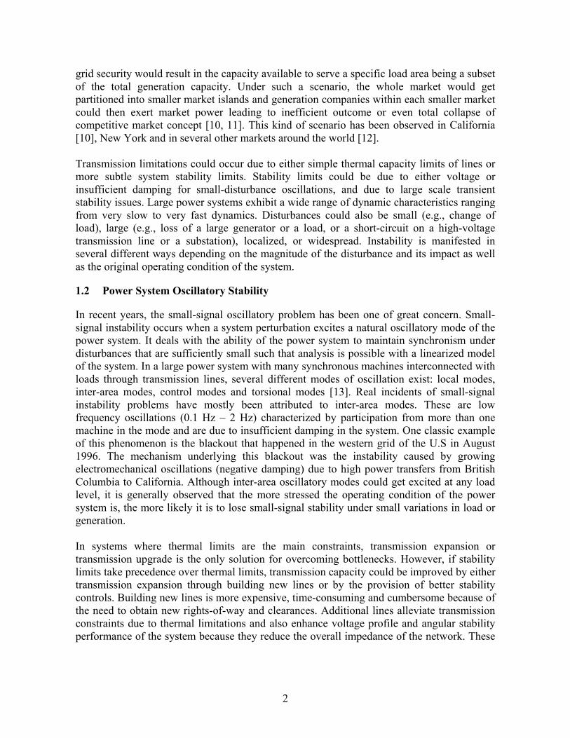
1.2 Power System Oscillatory Stability
In recent years, the small-signal oscillatory problem has been one of great concern. Small-signal instability occurs when a system perturbation excites a natural oscillatory mode of the power system. It deals with the ability of the power system to maintain synchronism under disturbances that are sufficiently small such that analysis is possible with a linearized model of the system. In a large power system with many synchronous machines interconnected with loads through transmission lines, several different modes of oscillation exist: local modes, inter-area modes, control modes and torsional modes [13]. Real incidents of small-signal instability problems have mostly been attributed to inter-area modes. These are low frequency oscillations (0.1 Hz – 2 Hz) characterized by participation from more than one machine in the mode and are due to insufficient damping in the system. One classic example of this phenomenon is the blackout that happened in the western grid of the U.S in August 1996. The mechanism underlying this blackout was the instability caused by growing electromechanical oscillations (negative damping) due to high power transfers from British Columbia to California. Although inter-area oscillatory modes could get excited at any load level, it is generally observed that the more stressed the operating condition of the power system is, the more likely it is to lose small-signal stability under small variations in load or generation. In systems where thermal limits are the main constraints, transmission expansion or transmission upgrade is the only solution for overcoming bottlenecks. However, if stability limits take precedence over thermal limits, transmission capacity could be improved by either transmission expansion through building new lines or by the provision of better stability controls. Building new lines is more expensive, time-consuming and cumbersome because of the need to obtain new rights-of-way and clearances. Additional lines alleviate transmission constraints due to thermal limitations and also enhance voltage profile and angular stability performance of the system because they reduce the overall impedance of the network. These

3
improvements would only be possible in the short-run with existing generation plants and load levels in the system. However, in the long-run, generating plants will be built and contracts will be established in such a way that the transmission capacity is used up to the maximum level and the system would again be operating close to the security limits [14]. When constraints are imposed due to stability limits, implementing better stability controls is a less cumbersome choice.
1.3 Power System Damping Enhancement
Power System Stabilizers (PSSs) [15] have been the most popular choice for the past two decades for small-signal stability enhancement. PSSs are continuous feedback-based controllers that add positive damping to generator electro-mechanical oscillations by modulating the generator excitation. One of the major limitations of conventional PSS is that of off-line tuning of the parameters in accordance with the operating condition of the system. Conventional PSSs are designed for particular operating points and their parameters need to be adjusted for effective damping at different operating points. A poorly tuned PSS could result in a destabilizing effect [13, 16, 17, 18, 19]. Often erratic performance is blamed on poor PSS tuning, resulting in PSSs being disabled by plant operators and leaving the system vulnerable to oscillatory instability. Conventional PSSs are predominantly local controllers on the individual generators, although on a theoretical level there has been some research on the use of global signals [20, 21, 22]. Use of local controllers to mitigate inter-area oscillations is known to have significant disadvantages. When multiple PSSs are installed at different machines, coordinating the actions of individual PSS is a serious issue and requires significant analytical and engineering effort. [17, 23, 24, 25]. A detailed study on the impact of interaction among different power system controls has been undertaken by Cigré Task Force TF 38.02.16. Several incidents of undesirable interactions among PSSs and other controls have been reported in [23]. Application of speed input or frequency input to PSS in thermal units requires careful consideration of the effects of torsional oscillations [17, 27]. The stabilizer, while damping rotor oscillations can cause instability of torsional modes. In addition, the stabilizer has to be custom-designed for each type of generating unit depending on its torsional characteristics. In recent years, with the advancements being made in fast power electronic switching technology, power electronics based controls collectively called FACTS (acronym for Flexible Alternating Current Transmission Systems) have generated a lot of interest. Several different control structures have been proposed for small-signal stability improvement using FACTS technology [26, 28, 29, 30, 31, 32]. Although these controllers have been shown to be quite effective in damping low frequency oscillations, there are several demerits associated with the use of FACTS devices for small-signal stability enhancement. One of the major demerits is the overall cost of installing the technology. The total investment cost for a single FACTS device of several 100 MVArs could be in the order of

4
tens of millions of dollars. Although FACTS devices are still cheaper than building new transmission lines, the overall cost of installing FACTS based controllers is massive. It is economically prohibitive to install FACTS devices only for small-signal stability performance. In fact, in some cases a carefully designed and properly tuned PSS has been shown to give a better damping performance compared to FACTS controllers [31]. Unless carefully designed and coordinated, most FACTS controllers offer only limited transient stability improvement. FACTS controllers have also been shown to have limitations with respect to robustness to system operating conditions [28, 30, 33, 34]. FACTS controllers need to be carefully coordinated among themselves as well as with other power system controls, especially excitation systems and PSSs if any. If not properly coordinated, FACTS based controls could adversely interact and cause instability [12, 23, 31, 35]. Independently designed FACTS controllers operating in the same electrical area have been shown to have destabilizing control interaction [12, 23, 36, 37]. It is extremely important to perform a coordinated design among all FACTS devices. From the above discussion, it is clear that the small-signal stability enhancement control measures currently in place fall short of robustness requirements. They present serious coordination challenges. They are often disabled when such careful coordination cannot be performed, leaving the system vulnerable to disturbances. FACTS based schemes are highly capital intensive. With deregulation, there have also been ownership and responsibility issues with respect to these controls that are discussed in Section 1.5. Robust non-capital intensive stability enhancement schemes that pose no complex coordination issues would be highly desirable. Control of active power loads for small-signal stability enhancement, as has been explained in Section 1.5, is inherently robust. Direct non-disruptive control of selected active power loads, if designed to be implemented with the existing distribution automation infrastructure, is highly cost effective. Although careful coordination of controllable loads is highly desirable for improved performance, lack of coordination would not result in seriously deteriorating performance. Market-based operation of loads, as detailed in Section 1.4, resolves ownership and responsibility issues related to security enhancement. With the availability of enabling technologies and an increased interest in demand side resources, direct non-disruptive control of loads is a very promising strategy for stability enhancement.
1.4 Load as a Resource
Load management programs in vertically integrated power systems have existed for many years. Section 2 in this report describes in detail these well-established practices with respect to load management in power systems. Utilities have in the past resorted to load shedding as well as interruptible load management for power system reliability only under extreme conditions. This practice was partly due to NERC’s definition of reliability. It encompasses two concepts: adequacy and security. Adequacy standards require that there be sufficient generation to meet the projected needs plus reserves for contingencies. Security standards require action by system operators to ensure that the system will remain intact even after

5
outages or other equipment failures occur. The traditional vertically integrated utility managed short-term reliability by dispatching its own generation. In competitive electricity markets, system operators responsible for maintaining reliability own no generation and must establish markets for reliability services. This change in the industry structure and the associated emergence of wholesale energy and reliability markets create new opportunities for demand-side resources. Under deregulation, the scope of load management programs has considerably broadened. With the emergence of deregulation, there have been tremendous developments in enabling technologies especially with respect to two-way communication, load control systems, monitoring, and metering. Today’s technology enables communication and control of several distributed resources almost in real-time and has been a major factor in the recent interest in demand-side resources. It is technically feasible for many distributed loads to simultaneously receive customized control signals. Load management programs are called demand response programs under deregulation and are designed and operated by the Independent System Operators (ISOs) or the Regional Transmission Operators (RTOs); they bring several new participants into the market such as retail suppliers, aggregators, curtailment service providers, etc. In 2002, the United States Supreme Court validated the authority of Federal Energy Regulatory Commission (FERC) over wholesale transmission sales and enabled the commission to dictate rules for competitive energy markets. Subsequently, in the same year, FERC proposed Standard Market Design (SMD) – a single set of market rules that would eliminate the differences between regional electricity markets and thereby standardize the U.S. energy market [38]. SMD is perhaps the most important step towards harnessing the benefits of competitive electricity markets and was developed by gathering “best practices” around the U.S. through an exhaustive stakeholder process. According to SMD, demand response is an important tenet in standardizing energy markets. SMD provides an appropriate platform for integration of demand response into the wholesale market structure [39]. In SMD, FERC strongly advocates demand participation on an equal footing with generation resources in order to achieve effective competitive performance in electricity markets [38, 39]. In fact, a load serving entity (LSE)’s ability to cut back on power use (i.e., demand response) when called by an ISO or an RTO will be considered equivalent to supply [38, 39, 40, 41]. This whole new perspective towards treating load as a system resource has sparked intense interest in the role for demand response in the efficient and reliable operation of deregulated power systems [42, 43, 44, 45, 46, 47, 48, 49, 50]. Demand response in the context of SMD is defined as load response called for by others and price response managed by end-use customers [51]. Load response includes direct load control, partial as well as complete load interruptions. Price response includes real-time pricing, dynamic pricing, coincident peak pricing, demand bidding and buyback programs. Demand response could be classified into two broad categories: market-based and reliability-based [52]. Market-based demand response programs enable efficient interaction of supply and demand for price stability. One of the earliest well-known works in the area of market-based control of loads was done by F.C. Schweppe et al [53]. Reliability-based demand

6
response programs are executed to provide network reliability services to the grid and its interconnected users. Market-based programs have reliability impacts and reliability-based programs do have price impacts. SMD states a clear preference for procurement of reliability services through the establishment of appropriate markets. In this regard, an SMD white paper [38] explicitly states that market rules must be technology as well as fuel neutral. They must not unduly bias the choice between demand or supply sources nor provide competitive advantages or disadvantages to large or small demand or supply sources. If the market rules are technology neutral, customer loads will be able to participate equally in providing reliability services. One problem in the wide-spread deployment of demand-side resources in the provision of reliability services is that the existing NERC policies inappropriately favor generation resources over customer loads [52]. NERC has recognized these limitations in its current operating policies, and is now considering amendments that would increase opportunities for demand-side resources [54]. Currently New York ISO, ISO New England, PJM, California ISO and the Independent Market Operator (IMO) Canada have a variety of demand response programs of market-based as well as reliability-based types [47, 48, 50, 52, 55, 56]. They are also actively investigating ways to improve the deployment as well as performance of demand-side resources from both economic and reliability points of view. References [55] and [56] provide a good summary of the various demand response programs at different ISOs and RTOs. There have also been several major research and development initiatives in the recent past, with the broader objective of enhancing the role of distributed end user resources. Two of the well-known initiatives are Consortium for Electric Reliability technology Solutions (CERTS) [57] and the Distributed Energy Program of the Department of Energy (DoE) [58]. The resources studied in these programs include loads, generation as well as storage at the distribution level of the power system. Several national laboratories have been actively pursuing research in the above areas. Prominent among them are the Energy & Engineering Division [59] as well as the Sensors and Electronics Division [60] of Pacific Northwest National Laboratory, Energy Efficiency and Renewable Energy Program of Oak Ridge National Laboratory [61], Electric Infrastructure Systems Research Program of National Renewable Energy Laboratory [62] and the Energy Analysis Program of Lawrence Berkeley National Laboratory [63].
1.5 Direct Load Control for Security Enhancement
The fundamental difference in the decision-making approach towards investment in power systems between a traditional vertical integrated power system and a deregulated power system has important implications in system stability related aspects. In a vertically integrated system, the approach was one of an integrated planning of generation, transmission, distribution and control additions. The objective was to achieve an optimum level of investment in each segment while maintaining a prescribed set of reliability

7
standards at minimum cost. However, in deregulated systems, the decision-making is highly decentralized. The Independent Power Producers (IPPs) make investment decisions in the generation segment based on the current market conditions as well as forecasts, among several other factors. IPPs also make the decision as to the type of generation to invest in. In recent years, there has been rapid progress in combustion turbine technology. Natural gas fired combined cycle plants constitute the large majority of additions that are continuing to be made in the generation sector. Their response characteristics differ substantially from conventional steam or hydro-turbine generating units [64, 65]. The primary objective of power producers in a deregulated system is control and optimization of their own resources. System reliability services, such as active reserves/frequency control, reactive reserves/voltage control and stability control are only secondary objectives. For example, use of higher cost generators with improved excitation systems and PSS would not be normally adopted by IPPs without hard rules to define compensation of associated costs involved. From the viewpoint of transient stability, IPPs may not be willing to participate in special protection schemes for the same reason and this may jeopardize system reliability. Also information exchange for modeling and analysis are more complicated in a market environment. The IPP could consider having no obligation to inform the others on what is occurring to its plant. It may not have adequate data acquisition capabilities. This withholding of information, either intentional or otherwise, could be detrimental to overall system reliability [Ch. 8 of 67]. The responsibility of system reliability and stability rests with the independent system operator, which although powerful does not own the resources that are necessary to ensure the availability of the above services. There is a need for a clear framework for the allocation of security costs to entities not contributing their share of reliability services. Setting aside ownership and responsibility issues, the associated technical problems related to stability themselves are potentially more complex in a restructured power system [66]. This can be attributed to several factors. Notable among these are an increase in the amount, geographical scope as well as frequency of changes in power flows, increased utilization of transmission, and the operation of the system closer to its limits. There is a strong need for effective, robust and adaptive control solutions in a deregulated system. The advancements in some of the enabling technologies for the demand-side briefly discussed in the previous section and detailed in Section 5 open up several new directions for power system stability enhancement and control. These advancements could be put to use in developing innovative, cost-effective solutions for stability enhancement, that make the best utilization of the existing infrastructure while not requiring major capital investments. Established competitive market frameworks have been developed or are in the stages of the development for demand side participation in related reliability resources such as active power reserves. With a clear preference by FERC for market-based solutions for the procurement of reliability services, control schemes for stability enhancement that make use of such competitive frameworks for load participation are attractive. Such market-based schemes enable resolution of issues related to the allocation of security costs. From a system reliability standpoint, customers could be viewed as willing to sell excess of reliability to the

8
power system operator in exchange for potential economic benefits through their participation in appropriate markets. Fundamentally, there are four different ways in which loads can make a significant contribution to the reliability of the bulk electric power system [44, 52]:
i) Ancillary service markets – Loads can bid in ancillary service markets. ii) Emergency operations – System operators can purchase bulk load reductions to
balance the system in the event of contingencies. iii) Installed capacity (ICAP) markets – Demand-side resources can address system
adequacy needs on a longer-term basis through participation in ICAP markets. iv) Transmission and distribution reliability – Loads can improve reliability of
transmission and distribution systems by improving angle stability, relieving congestion, enhancing voltage profile, and reducing overload on circuits.
The first three of the above aspects are under active investigation and development in today’s deregulated power systems. The interest in load participation in transmission and distribution system reliability enhancement is growing. In the initial stakeholder meeting of the New England Demand Response Initiative (NEDRI), created in 2002 to develop a comprehensive, coordinated set of demand response programs for the New England regional power markets, strong support was expressed for addressing this topic in the due course of the process [52]. The U.S. Department of Energy’s Bonneville Power Administration (BPA), which markets and delivers electricity in the Pacific Northwest region and operates one of the most reliable transmission grids in the world, has recognized the potential behind direct load control for angle stability enhancement [68] and has identified it as one of the key R&D directions. Underscoring the importance of research on this topic, a new task-force on fast-acting load control for system and price stability was formed in 2001 within the Power System Dynamic Performance committee of the IEEE Power Engineering Society [69]. This task-force addresses many aspects including commercial arrangements, communications requirements, security assessment and different load characteristics. Pacific Northwest National Laboratory is actively investigating the use of distributed, fast acting load control for frequency stability [59]. The following are some desirable characteristics for loads that could be considered as candidates for control [42]:
a) Storage: A controllable load should have some storage in its process, typically in the form of productive effort in which the load is engaged.
b) Control capability: A controllable load should have the capability to respond to disconnection and reconnection requests. Loads with control systems that can be adapted to respond to such requests are good candidates.
c) Response speed: Rapid response requirements are desirable. d) Size: Aggregate size is important. The size of the aggregate resource needs to be large
enough to be useful. Large loads are easier to monitor and small resources behave statistically and potentially have higher reliability as a group.

9
e) Minimal cost: Loads are not specifically designed to respond to power system needs. It is desirable that adding additional capabilities for the load is not costly.
The control strategy, the dynamic performance improvement possible through load control, and the amount and type of disruption caused to the customer depend on the type of the load being controlled. Under deregulation, there is a strong need to possess tools and techniques for security assessment that produce operating limit boundaries for both static and dynamic security of power systems. Knowledge of such operating limits a priori would enable the system operator to efficiently procure services that are necessary to operate the system securely. Besides, an increase in overall uncertainty in operating conditions makes corrective actions at times ineffective, leaving the system vulnerable. Tools and techniques currently available for stability enhancement are mostly corrective in nature, and lack robustness to operating condition changes, as discussed in the previous sections. The approach developed in this research is based on preventive control of distributed loads in order to improve system dynamic performance. Based on the desirable characteristics of loads for control applications as mentioned above, the following loads have been selected as controllable: residential and commercial air conditioner/heating loads and water-heater loads. Direct load control for stability enhancement is based on the fundamental premise that the cumulative effect of controlling several individually insignificant loads distributed geographically and electrically, provides sufficient leverage for the system to be operated securely at times when the system is vulnerable. By selecting loads to be controlled appropriately and by optimizing the time duration for control action for each load, it is possible to accomplish secure operation while minimizing the amount of disruption to the customer. The control strategy involved in activating load control will have significant bearing on the overall system reliability. The type of load to be controlled and the performance improvement that could be obtained greatly influence the control strategy. Non-critical loads could be controlled selectively, leaving critical loads uninterrupted. As a comparison, a power system stabilizer modulates excitation, thereby the reactive power generated, to effect a change in the terminal bus voltage which in turn affects the nearby voltage dependent loads as well as power transfer. These two effects could be of comparable magnitude [34]. Depending on the system operating condition, they could be additive or could counteract each other. The net impact of this modulation is thus unpredictable and to a large extent depends on operating conditions. An SVC operates in the same way. On the other hand, control of active power loads is a direct way of controlling power flows. Hence the scheme is inherently robust. In a practical power system, the number of dominant oscillatory modes is often larger than the number of control devices available to control them. The robustness with regard to direct load control implies that it is conceptually possible to damp out different inter-area modes that get excited at different power flow levels.

10
In modulating loads with appropriately designed algorithms, much of the existing infrastructure for demand side management could be made use of. Control of loads at the distribution level would not require new installations at the high voltage level. The additional investment needed in most cases would not be massive.
1.6 Objectives and Scope of the Research
This research proposes robust oscillatory stability enhancement through cost-effective, direct, non-disruptive control of loads. The control strategy for load control is preventive in nature. The objective of this research is to address the following broad issues with respect to control of loads:
• The type of loads to be controlled • A fundamental analysis of the framework and different approaches based on the
framework to decide on optimal location and amount of load to be controlled, in order to achieve a desired damping performance for the entire power system
• Modulation of loads to achieve improved system damping in the presence of uncertainty in loads as well as in generation
• Strategies used to control different loads so that the desired stability performance is maintained in the system while causing minimum disruption
• The effect of various extraneous variables on the effectiveness of load control. The underlying framework for analysis to determine the optimal amount of load to be modulated is based on the Structured Singular Value (SSV or μ) theory. The SSV theory in robust control [119, 121] offers a powerful technique to analyze robustness as well as design controllers that satisfy robust performance for linear control systems with uncertainties that can be represented in a structured form. It has previously been successfully applied in analyzing stability robustness [132, 133] of power systems and in designing robust PSS and SVC damping controllers [134, 135]. In this research, the setup for uncertainty characterization in power systems developed in [132] has been extended to develop a robust performance analysis framework. Robust performance analysis deals with the determination of maximum uncertainty bounds for which the system satisfies desired performance specifications. Robust performance analysis is performed through the application of the robust performance theorem [122]. The scope of this research work includes the following:
1. Development of a linear model for the problem of direct load control. This linear model would serve as the basis for the analysis framework. It would also be applied in selecting the optimal locations for load modulation through a comprehensive modal analysis. The important difference between a linear model for direct load control and those used in other power system control designs is the fact that the load available for control at a bus is modeled as an input to the system. This allows the use of different load models for controllable load at each load bus and is essential to characterize the uncertainty in the controllable part of the load.
11
2. The linear model developed for direct load control is cast into a framework suitable
for the application of the robust performance theorem, one of the fundamental theorems related to SSV concept. The uncertainty in the operating conditions in terms of load levels or generation is real-parametric uncertainty and could be represented in a structured form thereby making it possible for SSV-based analysis. A framework for robust performance analysis is developed from a Linear Fractional Transformation (LFT) representation of uncertainty in the state-space model and the damping performance specifications in terms of the MIMO H∞ norm.
3. The objective of robust performance analysis is to determine load levels at buses
selected for control implementation, which would satisfy the desired performance specifications. Depending upon the uncertainty characterization as well as the robust performance analysis problem formulation, there are two fundamentally different approaches to an analysis of the above problem.
(a) Determination of worst-case uncertainty for a given performance specification –
In this formulation of the problem, active power load at each load bus selected for control is assumed to be the sum of controllable and uncontrollable parts. Uncertainty is assumed to exist in the controllable part of the loads. The analysis then proceeds to determine the maximum uncertainty range for the controllable as well as the total load levels that satisfies the damping performance specifications. It has been analytically shown that with the above uncertainty characterization and the criterion for performance specification satisfied, it is always possible to determine the maximum uncertainty range in load levels that would satisfy the chosen performance conditions.
(b) Determination of worst-case performance for a given uncertainty range – This
approach, in principle, is similar to NASA’s patented on-line μ method for robust flutter prediction for air-craft models [145]. This is a fairly general formulation of the problem and it allows uncertainty to exist not only in load levels, but in generation levels as well as in any parameter of the system. However, the uncertainty bounds are assumed to be fixed. To start with, for the given uncertainty range, the worst-case performance is computed. If it does not satisfy the desired specifications, the algorithm modulates the load levels at selected load buses in the system. The load modulation is iterative and is performed until the load level in the system is such that the chosen performance specifications are satisfied for the uncertainty range under consideration. The selection of load buses for control implementation is based on the eigenvalue sensitivity of active power loads.
Both the above formulations are skewed – μ formulations in the context of SSV theory [144]. The first approach is applied with variable load uncertainty bounds and the second approach is applied with uncertainty in load, generation, or in any other system parameter, however, with fixed bounds.

12
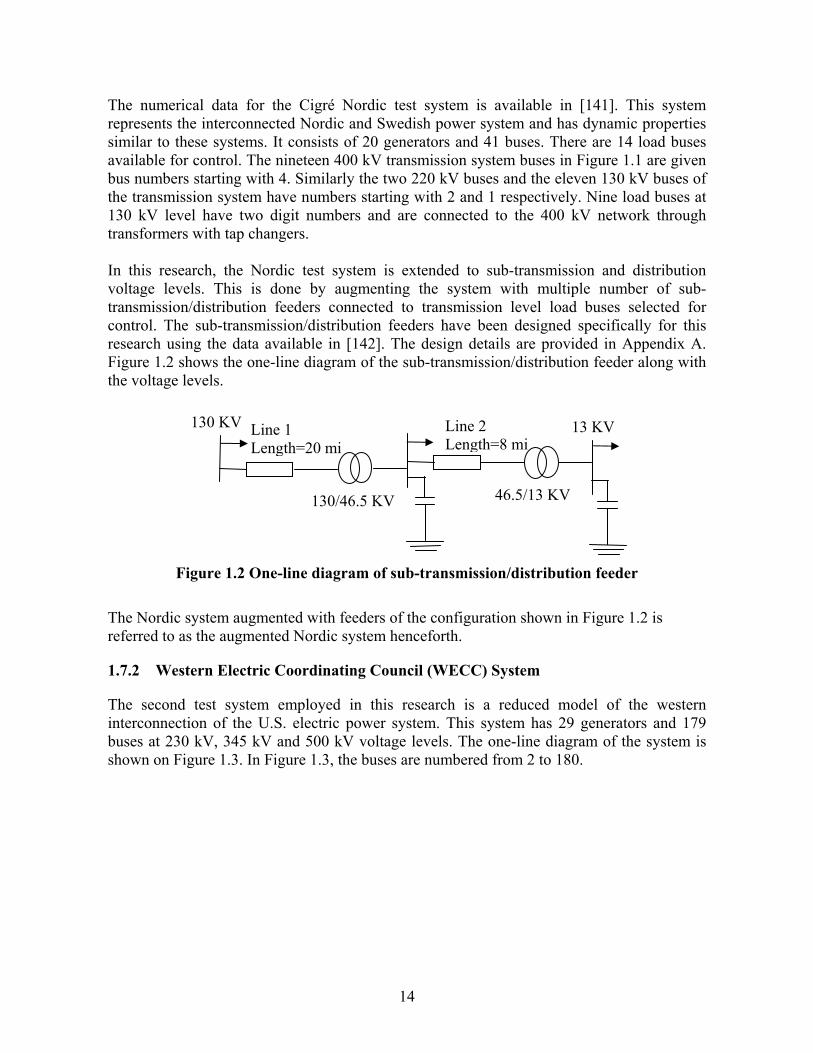
In the determination of load levels that satisfy the chosen damping performance conditions, the analysis could be done at the transmission level of the system. The amount of load to be modulated at the transmission level could then be divided amongst multiple feeders that connect at the transmission level load bus. Alternatively, the system at transmission voltage level could be augmented with sub-transmission and distribution systems and the determination of the amount of load to be modulated could be done at the distribution level. Both these approaches have been illustrated.
4. Develop algorithms for operating controllable thermal loads – air conditioners and water heaters – based on the results of the analysis problem described above. In controlling the group of thermostatically driven loads, the phenomenon of cold load pickup needs to be modeled and taken care of. Also, control needs to be distributed among several groups of loads available for control. The objective is to operate the loads with minimum disruption or discomfort, while maintaining the load levels such that the desired performance conditions are satisfied. Two different algorithms based on Dynamic Programming with different sets of constraints are proposed for air-conditioner loads, while a decision-tree based algorithm is proposed for water-heater loads. The development of these algorithms is in line with some of the most recent load management programs executed.

13
1.7 Test Systems
1.7.1 Cigré Nordic (Nordic32) System
Figure 1.1 One-line diagram of Cigré Nordic system
PV PV PV
N20
32
PV
PV
PV
PV
PV PV
PV
PV
PVPV
PV
PV PV
N407 N401
N407 N401
N101
N101
N101
N101
N10
21
N102 N40
2 N4021
N20
3
N40
3
N40
3N404
N4
PV
N40
43
N40
46
N4
N46
N
404
N40
44
N10
4N
104 N
1044
N10
4
N10
4
N41
N406
N61
N406
N6
N40
51
N51
N40
47
N47
N404
N6
N406
PV
PV
14
The numerical data for the Cigré Nordic test system is available in [141]. This system represents the interconnected Nordic and Swedish power system and has dynamic properties similar to these systems. It consists of 20 generators and 41 buses. There are 14 load buses available for control. The nineteen 400 kV transmission system buses in Figure 1.1 are given bus numbers starting with 4. Similarly the two 220 kV buses and the eleven 130 kV buses of the transmission system have numbers starting with 2 and 1 respectively. Nine load buses at 130 kV level have two digit numbers and are connected to the 400 kV network through transformers with tap changers. In this research, the Nordic test system is extended to sub-transmission and distribution voltage levels. This is done by augmenting the system with multiple number of sub-transmission/distribution feeders connected to transmission level load buses selected for control. The sub-transmission/distribution feeders have been designed specifically for this research using the data available in [142]. The design details are provided in Appendix A. Figure 1.2 shows the one-line diagram of the sub-transmission/distribution feeder along with the voltage levels.
Figure 1.2 One-line diagram of sub-transmission/distribution feeder
The Nordic system augmented with feeders of the configuration shown in Figure 1.2 is referred to as the augmented Nordic system henceforth.
1.7.2 Western Electric Coordinating Council (WECC) System
The second test system employed in this research is a reduced model of the western interconnection of the U.S. electric power system. This system has 29 generators and 179 buses at 230 kV, 345 kV and 500 kV voltage levels. The one-line diagram of the system is shown on Figure 1.3. In Figure 1.3, the buses are numbered from 2 to 180.
130/46.5 KV
Line 1 Length=20 mi
13 KV Line 2 Length=8 mi
46.5/13 KV
130 KV

15
.
Figure 1.3 One-line diagram of WECC system

16
1.8 Outline of the Report
This report consists of 7 sections. Section 1 provides the background and motivation as well as an introduction to the problem. The objectives and scope of this research have been described in detail. The test systems used in this research have been introduced along with their one-line diagrams. Section 2 provides a detailed summary of the literature review undertaken for this research. The relevant literature has been segregated and discussed as shown below:
• Section 2.1 reviews literature related to traditional load management in power systems. This section consists of two sub-sections. Within the broader topic of traditional load management, literature related to emergency load shedding has been discussed in section 2.1.1 and that related to direct load control had been discussed in Section 2.1.2. Literature on direct load control has been segregated further and discussed in Sections 2.1.2.1 and 2.1.2.2. Section 2.1.1.1 discusses literature related to cold load pickup and physically based modeling of loads. Section 2.1.1.2 discusses literature on stochastic aggregation of loads.
• Section 2.2 reviews literature on direct load control applied for damping enhancement.
• Section 2.3 reviews literature on the application of robust control techniques in power system control design and analysis.
Section 3 presents a detailed derivation of the state-space linear model of the power system for the problem of load control. It has been organized as follows:
• Section 3.1 provides a description of the mathematical models of power system components and dynamic equations corresponding to the models.
• Section 3.2 presents the algebraic equations for the purpose of deriving the linear model.
• Section 3.3 presents the differential algebraic set of the overall system equations. • Section 3.4 presents the step-by-step linearization procedure and the linear model
derived. Section 4 deals with the development of an analysis framework for load modulation based on structured singular value theory. The necessary mathematical concepts have been presented in detail followed by the development of the analysis framework. This section is organized as follows:
• Section 4.1 presents a brief historical overview of the development of structured singular value theory in the area of robust control.
• Section 4.2 discusses different ways of characterizing uncertainty in physical systems. The uncertainty characterization and its basis for the problem at hand have also been briefly discussed.
• Section 4.3 discusses in detail the concept of structured singular value. The definition of structured singular value and the necessary background have been presented.
• Section 4.4 discusses linear fractional transformation (LFT), an important concept

17
related to performing analysis and design for robust control. The problem of well-posedness of LFTs, formal definition of LFT, and the basic principle behind the application of LFTs have been discussed in sub-sections 4.4.1, 4.4.2 and 4.4.3 respectively.
• Section 4.5 discusses robust stability and a theorem on robust stability. • Section 4.6 discusses robust performance and a theorem on robust performance. • Section 4.7 discusses the concept of skewed – μ and its relevance to the load
modulation analysis approaches presented later in Section 5. • Section 4.8 presents a description of the development of SSV-based analysis
framework for robust performance. It has been organized into the following sub-sections: Section 4.8.1 provides a detailed treatment of the characterization of parametric
uncertainty in the state-space model of the power system developed in Section 3. The different sources of parametric uncertainty have been presented followed by the representation of uncertainty in LFT form.
Section 4.8.2 deals with characterization of small-signal stability performance in the analysis framework through the choice of appropriate error signals. Simulation results with the linear simulation tool, SIMGUI, available in Matlab μ – toolbox for the augmented Nordic system and the WECC system have been presented in sub-sections 4.8.2.1.1 and 4.8.2.1.2.
Section 4.8.3 presents the development of the analysis framework through the application of parametric uncertainty and performance characterizations.
Section 5 deals with two different skewed – μ based robust performance analysis approaches for load modulation that are based on the framework developed in Section 4. This section has been organized as follows:
• Section 5.1 presents a detailed description of modal analysis using eigenvalue sensitivities for the selection of appropriate locations for load modulation.
• Section 5.2 provides a comprehensive overview of the robust performance analysis approaches proposed in this section. The basis for the two different approaches developed as well the conceptual difference between the two approaches has been clearly outlined. The relevance of the robust performance analysis problem to the concept of skewed – μ and its implications have also been discussed.
• Section 5.3 deals with approach I for load modulation analysis – determination of worst-case uncertainty for fixed performance. The basic assumptions and fundamental aspects related to this approach and the analytical background have all been explained in detail. In addition, an analytical proof of the correctness of the approach has been presented. Section 5.3.1 presents the algorithm for approach I. Numerical and simulation results for approach I on the augmented Nordic system and the WECC system have been presented in Section 5.3.2.
• Section 5.4 provides a detailed treatment of approach II for load modulation analysis – determination of worst-case performance for fixed uncertainty. The algorithm for approach II has been described in Section 5.4.1. Numerical and simulation results for approach II have been presented for the WECC system in Section 5.4.2.

18
Section 6 deals in detail with different specialized algorithms developed for real-time modulation of loads. This section consists of the following four parts:
• Section 6.1 presents a detailed overview of the background for the load modulation algorithms proposed in this section. A brief historical overview of load control technology, recent developments in load control systems as well as some recent applications of the above technologies in different utilities in the U.S. have been described.
• Section 6.2 provides a description of the optimization framework developed to study air-conditioner load control. The air-conditioner load model, the basic setup assumed for the optimization problem, and the dynamic programming based optimization problem have all been explained in detail. The basis for Monte Carlo simulation and the uncertainties assumed in performing Monte Carlo simulation have also been explained. Monte Carlo simulation results have been provided with two different types of constraints introduced in the optimization problem, constraint on cycling times, constraint on internal temperature excursions. The impact of constraints as well as various parameters and variables have been studied in these results. A qualitative discussion of the results with the different DP algorithms has also been provided.
• Section 6.3 describes the development of an optimization framework to study the control of water-heaters. The model of a domestic water-heater assumed for this work has been explained followed by a decision-tree based control algorithm developed through the application of the model. Two different approaches to arrive at the data required for implementing the algorithm have also been dealt with. The algorithm has been illustrated with a numerical result.
• Section 6.4 provides a high-level overview of the direct load control framework based on the algorithms proposed in this section.
Section 7 provides a summary of specific contributions of this research as well as suggestions for future work.

19
2. Literature Review
2.1 Traditional Load Management in Power Systems
2.1.1 Emergency Load Shedding
In general, the operation of a power system can be characterized by five different operating states, namely normal, alert, emergency, in extremis and restorative states [9]. A system operating in the normal state could slip to an alert state upon the occurrence of quite a severe disturbance or a drastic change in loading conditions. It could further slip to an emergency state, upon the occurrence of a severe disturbance when in the alert state. In an emergency state, the voltage violations and frequency deviations are beyond their respective acceptable limits and/or equipment loadings exceed their short-term emergency ratings. However, the system as a whole is still intact. It is under such a condition that tripping of load is usually resorted to as one of several emergency control actions. This has been an established practice to bring the system back to the alert state, but with reduced load being served in the new alert state. The main objective of tripping load when in the emergency state is to bring the frequency back to within acceptable limits or improve the voltage profile and prevent voltage collapse. Thus there are two very popular load shedding schemes, under-frequency load shedding [70] and under-voltage load shedding [71]. Considerations in the selection of the scheme include the maximum generation deficiency for which protection is required, the minimum permissible frequency, and the range of inertia constant and load damping constant [72]. The characteristics and locations of the loads are more important for voltage problems than they are for frequency problems [9]. In some other instances, load shedding could also be done in order to maintain transient stability. One such scheme used by U.S. Northwest Power Pool to maintain transient stability of the Western Electric Coordinating Council (WECC) systems is described in [73]. Load shedding is also used with controlled separation upon detection of an impending instability. Controlled separation is initiated by opening the appropriate tie lines before cascading outages can occur. In such instances, it may be necessary to shed loads to balance generation and load in the separated systems [74].
2.1.2 Direct Load Control
The other type of load management that has been in practice since the 70’s is direct load control for reducing operating costs as well as maintaining system reliability [75, 76, 77, 78, 79, 80]. Utilities in the vertically integrated structure have offered incentives in return for allowing direct control of a selected group of customer loads. Loads under direct control can be selectively controlled as needs require [81]. The term “direct” is used because the control is exerted directly, moment-to-moment, by the utility using a communication line. This is in contrast to indirect control through incentives or devices such as thermal storage which are outside the direct control of the utility. The objectives of such a scheme have been manifold, such as reduction of system peak, improvement of load factor, defer or reduce the need for generation capacity from peak to off-peak hours, reduction of operating cost, reduction of losses in the feeders, or provision of contingency reserves. Various algorithms have been

20
proposed in order to optimize the amount of load management with different objectives. Dynamic programming based approaches have been quite popular [80, 82, 83, 84]. Fuzzy logic and linear programming based algorithms have also been proposed [76, 85, 86]. A detailed treatment of these algorithms has been provided in Section 5 of this report. There is a variety of economic as well as reliability issues that will have to be taken into consideration in formulating a load management strategy. These issues are utility-specific. The usual practice is to assess in detail several multiple strategies and then choose the most economical strategy or a combination of strategies [77].
2.1.2.1 Cold Load Pickup and Physically based Modeling of Loads
The usual types of loads controlled in load management programs have been thermostatically driven loads such as air-conditioners and space-heating and water-heater loads. In some schemes for provision of contingency reserves, control of municipal water-pumping loads has been proposed [87]. Due to the stochastic nature of thermostatic loads, it is essential to study the load dynamic response during and after control periods in order to assess the impact of a load management program on power system performance. When an aggregate of thermostatically driven loads is switched off, there occurs a surge in the total load when they are switched back to service [88]. This phenomenon is called cold load pickup and is essentially the result of loss of diversity among thermostatically driven loads. This was first identified as a potential problem in 1949 when Audlin et al presented the results of a staged outage in Syracuse, New York [89]. It is one of the most studied aspects in distribution system design and analysis. In order to take into account the effect of cold load pickup in a load management study, the load equipments will have to be modeled accurately by physically based models. Such models capture the physics of operation of the equipments and predict the response to control actions. Several physical models have been proposed for studying cold load pickup in both air-conditioners and water-heaters . In one of the earliest attempts, Galiana et al [90] proposed an empirical method for predicting physical load. This method lacks a mathematical formulation. It is not suitable for short-term load prediction, but could be used for long-term load management. In 1981, Ihara and Schweppe [91] presented a dynamic model for the temperature of a house that is heated by a thermostatically driven heater. This model is fairly simple and has been proven to capture the behavior of thermal loads accurately. Several refinements of this model are available in the literature. In [92], this model has been converted into a sample-data form by discretizing time and has been used to study the aggregate load behavior. Actual utility data is examined and it has been identified that the recovery transient has two epochs. Five different heating load models with different characteristics to model the two epochs have been studied. Reference [93] suggests the development of a residential load model based on physically based simulation. Reference [94] proposes a lumped parameter model of an air-conditioner with the parameters determined through system identification techniques such the as maximum likelihood principle. In [95], the thermodynamic behavior of a house is modeled using a parallel RC circuit. Door openings and other small heat flows are modeled as a random current source in the circuit. A stochastic model for heating and cooling loads is presented in [96]. This model

21
includes the random influences in the environment through the introduction of discrete white noise term. It is used to study the effect of stochastic characteristics of different parameters of the model developed in [91]. Reference [97] presents a detailed model for air-conditioning loads by capturing weather effects more accurately. The effects of humidity and solar radiation in the model for air-conditioning are represented in [98]. Reference [99] suggests the importance of modeling the stochastic aspects of lifestyles in the development of physically-based load models. References [100, 101, 102, 104] present different physically-based models of electric water-heating loads. Development of water-heater models is based on water-heater usage pattern as well as the physics of water-heating. Reference [103] simulates actual control scenarios through the application of the model developed in [100]. It has been shown that [100] captures the response to control actions quite accurately.
2.1.2.2 Stochastic Aggregation
With individual equipments modeled in sufficient detail, the behavior of a group of such loads could be studied through simulation. However, there have also been several stochastic techniques proposed to aggregate individual thermostatically driven loads. Reference [104] presents stochastic aggregation of a group of water-heater loads. The resulting model is a “traveling” wave model. In [94], with the assumption that the switching processes are ergodic, the mean duty factor as well as the sample variance of duty factor for a group of air-conditioner loads are calculated using Kalman Filter expressions. The aggregate model is further applied to study energy consumption, voltage response etc. Reference [97] develops an aggregate model of a group of air-conditioners based on an analogy between lumped parameter heat flow problems and lumped parameter electric circuits. It has been shown to closely model the aggregate demand as well as energy payback effect after an outage. In [95], aggregate dynamics for a homogenous group of devices are derived as a set of Focker-Planck equations –system of coupled ordinary partial differential equations. A perturbation analysis yields the dynamics for a non-homogenous group.
2.2 Direct Load Control for Damping Enhancement
Power system small-signal stability improvement through the control of active power loads was suggested as early as in 1968 by R.H. Park [111]. However, this concept was not investigated closely until the mid 90’s, possibly because of a lack of enabling technologies. Damping of electro-mechanical oscillations through the control of active power loads was first studied in detail in [112]. References [113, 114, 115, 116] are based on [112]. With respect to the application of direct load control for stability enhancement, [112] examines modal analysis for the selection of load buses for control implementation, selection of appropriate feedback signals for the load controller that capture the poor damping characteristics, type of load controller for load modulation, controller design and practical considerations in implementing direct load control for oscillatory stability enhancement. The entire power system with all component models is represented by a time-invariant differential algebraic system of equations (DAE). Selection of the best location for implementing load control is based on both the active power controllability as well as eigenvalue sensitivity for
22
the poorly damped modes under consideration. The following feedback signals are proposed: local bus frequency, frequency of the closest machine and estimated mode frequency. All of these signals are local signals. The type of controller is based on the structural knowledge of the physical behavior rather than on strong mathematical principles. The control law applied is the modulation of real power injection proportional to local bus frequency, which is analogous to viscous damping in mechanical systems. The modulation of load is performed at the transmission level of the system. It has also been shown in [116] that on-off modulation is more effective than sinusoidal modulation proportional to frequency for large oscillations. However for small oscillations, sinusoidal modulation is found to be more effective. Different structures and locations of measurement points and actuators are listed. When control is implemented at two load buses, the gains for the two controllers are selected sequentially. However, it is found that a new mode is introduced with multiple controllers and the overall system damping may be reduced although individual modes could be well damped with two controllers. Reference [117] deals with large-scale active load modulation for angle stability improvement. The control scheme is based on the use of global feedback signals for the controller. Both continuous and discontinuous modulation schemes have been proposed. The controller designed for continuous modulation is a two-loop active power stabilizer presented in [118]. A fully decentralized two-loop active power stabilizer uses local frequency deviation to stabilize the poorly damped low frequency mode that is introduced due to the hydraulic turbine and the speed governor. It uses local bus voltage to stabilize the dominant system mode. However, when this scheme based on using local bus measurements was tested on the Hydro-Quebec power system, it was found to be ineffective in stabilizing a realistic configuration of the network. Also it was found that there was a strong coupling between bus voltage and bus frequency resulting in interaction between the two loops. Based on these initial investigations, the use of global signals has been suggested. The discontinuous modulation scheme is based on an empirical, four-level, fixed-shedding which covers a given time-frame following fault inception. The discontinuous modulation scheme is combined with a continuous modulation scheme for application. Further, this work also mentions four important design factors in the load modulation scheme (upper limit of the actuator, communication delay, amount of controllable load, and control accuracy) and studies the sensitivity to the first two. Conclusions based on this sensitivity study are that the continuous modulation scheme is quite sensitive to communication delays; the discontinuous modulation has been found to be robust to such delays. However, the continuous modulation is more energy-efficient and requires lesser load modulation compared to the discontinuous scheme. These earlier works for damping enhancement are based on corrective control. A common assumption is that the control of individual sub-transmission and distribution level feeder loads is properly coordinated so that a continuous modulation of active power is possible at the transmission level bus where the different feeders connect. Unlike control on the generation, load control is inherently discrete. The control of individual discrete blocks of load, at sub-transmission and distribution levels of the system, will have to be carefully coordinated in order to result in a smooth modulation of active power at the transmission level. This coordination is critical to the effectiveness of control. It is not straight-forward to
23
achieve and has not been dealt with in any of these works. Also, in corrective control strategy with continuous modulation, it is clear from the results that the response time requirements and communication delay limits are extremely stringent [117]. These may be unreasonable to achieve in practice. There are requirements for power electronics based fast switching to enable smooth active power modulation making the overall installation highly capital intensive. There have been no general guidelines proposed for the selection of input signals for the controllers. When multiple controllers are used, or when multiple loops are used in a load stabilizer, the possibility of undesirable interaction has been shown to exist. A careful sequential tuning of gains has been suggested for this problem. Reference [117] uses a so-called modal performance index measure for optimal selection of the parameters for the stabilizer. As far as discontinuous modulation is concerned, it is based on heuristics; it is highly system-specific. Although it has been shown to be effective for certain operating conditions, the robustness is not demonstrated. The continuous modulation schemes based on simple root-locus design as well as the two-loop decentralized stabilizer design also lack robustness. The phase adjustment of the stabilizer transfer function could differ widely from one oscillatory frequency to the other. The solution suggested in [117] is the simultaneous use of several transfer functions combined in a multi-loop scheme, each targeting the damping of one particular mode.
2.3 Robust Control Applied to Power Systems
The evaluation of robustness has been one of the major preoccupations in the design of control schemes for power systems. Electric power systems are non-linear and time-varying dynamical systems. However, most of the control design techniques, classical as well as modern, are based on the use of linear models. Considerable level of uncertainty is introduced as a result of operating the system at conditions for which the control systems were not designed for. Uncertainty exists even with no changes in operating conditions. Often there are system parameters and those that correspond to the equipment that cannot be known exactly, but need to be estimated; these estimates could be erroneous. The synchronous generator electrical as well as certain mechanical parameters, the excitation system time-constants, load model parameters are some examples. In real-time operation of the system, forecasts and measurements usually have margins of uncertainty. Accurate power system dynamic models are usually of a very high order, and often to reduce the dimensionality, model order reduction is resorted to. This introduces a significant amount of uncertainty. This problem of successful design of system operation schemes in the presence of uncertainties is quite a challenge. Since the early 80’s, extensive research has focused on the analysis and design of control systems in the presence of uncertainty. This has led to the development of modern robust control, a whole new area within modern control systems. Today, robust control is a well established discipline, with MATLAB toolboxes. It deals with stability and performance validations of uncertain linear control systems. Several of the tools and techniques developed in robust control have shown a lot of promise for application to power system analysis and control design. Different techniques investigated include Kharitonov’s theorem, interval analysis, L1, H∞, L∞, the Structured Singular Value (µ) theory, and Loop Shaping and

24
Linear Parameter Varying (LPV) theory-based techniques [123 – 138]. Kharitonov’s theorem has been applied to the design of a robust power system stabilizer in [123]. References [124, 125] deal with robust stability analysis using the L∞ technique. The H∞ optimization approach has been applied for power system controller synthesis in [126, 127, 128, 129, 130]. The main demerit of H∞ based control design is that it is restricted to multiplicative and/or additive uncertainty and this leads to conservative controller designs. The Structured Singular Value theory is advantageous when the uncertainty could be represented in a structured form. Parametric uncertainties in power systems are structured uncertainties and the SSV theory has been successfully applied in power system stability analysis as well as in controller synthesis in [132, 133, 134, 135, 136]. PSS design using Glover McFarlane loop shaping approach has been presented in [137]. More recently, the application of the LPV theory in power system stabilizer design has been presented in [138].

25
3. Power System Linear Model for Load Control
The tools and techniques of modern robust control, including the Structured Singular Value theory, are all applicable to linear control systems. The foundation for analysis and design using these techniques is a linear model of the uncertain control system. The linear model together with proper uncertainty characterization is expressed in a form suitable for the application of robust control techniques. In this section the linear model suitable for application of Structured Singular Value based robust performance analysis for the direct load control problem is derived. The following approach is adopted to build a linear model of the power system for the load control problem: Each individual component in the system is modeled in sufficient detail with its dynamic model. These individual dynamic models are coupled together through the network algebraic equations using a common reference [139]. Linearizing the system involves eliminating the algebraic variables corresponding to the network, resulting in a linear model that relates the derivative of the states with the states and the inputs. The linear model developed in this section for the load control problem is different from other linear models used in power system control design. The difference is that, in the model development, the total active power load at certain candidate load buses is assumed to be the sum of controllable and uncontrollable parts. The controllable parts of the load at such load buses are then modeled as system inputs. This facilitates the following:
i) Characterization of uncertainty in the controllable parts of the loads for the development of analysis framework
ii) Calculation of eigenvalue sensitivity and active power controllability for load inputs, which are used in the selection of optimal locations for load modulation
iii) The use of different load models for the controllable and uncontrollable parts of the load.
The functional notation of the differential algebraic system of equations that describe the power system is as follows:
U)Y,G(X,0U)Y,F(X,X
==&
(3.1)
where X and Y are the vectors of state variables and algebraic variables, respectively; F and G are functions of X and Y.
Linearizing the above set of equations around an operating point,
ΔUUFΔY
YFΔX
XFXΔ
∂∂
+∂∂
+∂∂
=& (3.2)
ΔUUGΔY
YGΔX
XG0
∂∂
+∂∂
+∂∂
= (3.3)

26
From (3.3)
ΔUUG1
YGΔX
XG1
YGΔY
∂∂−
⎥⎦⎤
⎢⎣⎡∂∂
−∂∂−
⎥⎦⎤
⎢⎣⎡∂∂
−= (3.4)
Substituting for ΔY in (3.2) yields
ΔUUG1
YG
UFΔX
XG1
YG
XFXΔ
⎥⎥⎦
⎤
⎢⎢⎣
⎡
∂∂−
⎥⎦⎤
⎢⎣⎡∂∂
−∂∂
+⎥⎥⎦
⎤
⎢⎢⎣
⎡
∂∂−
⎥⎦⎤
⎢⎣⎡∂∂
−∂∂
=& (3.5)
= UBΔXAΔ + (3.6)
3.1 Dynamic Equations
3.1.1 Generator Model
3.1.1.1 Two-axis Model
In this research, generators have been modeled by the two-axis model [139]. The two-axis model for a generator accounts for the transient effects in flux, while the sub-transient effects are neglected. The transient effects are dominated by the rotor circuits, which are the field circuit in the direct (d) axis and an equivalent circuit in the quadrature (q) axis formed by the solid rotor. Following are the two key assumptions made in this model:
i. In general, the stator voltage generated is the sum of two parts: speed voltage part and the part corresponding to the rate of change of flux. The two-axis model makes the assumption that the part corresponding to the variation of flux-linkages of d- and q-axes is negligible compared to the speed voltage part.
ii. 1=≅ Sωω The dynamic equations corresponding to the two-axis model are given by:
( ) iiiiii qqqddq IxxEEτ ′−+′−=′′ &0 (3.7)
( ) iiiiiii dddqFDqd IxxEEEτ ′−+′−−=′′ &0 (3.8)
)ω(ωDI)Ix(x)EIE(IPωM siidqqqqqddmi iiiiiiiiii −−′−+′+′−= (3.9)
sii ωωδ −=& (3.10)
i=1,2,…,Ng
where
A

27
:, qd EE ′′ d-axis and q-axis stator EMFs corresponding to rotor transient flux components, respectively
Id, Iq: d-axis and q-axis stator currents
:00, qd ττ ′′ open-circuit direct and quadrature axes transient time-constants
:, dd xx ′ direct axis synchronous and transient reactances
:, qq xx ′ quadrature axis synchronous and transient reactances
EFD: stator EMF corresponding to field voltage
Di: damping coefficient of generator i and
Ng is the total number of generators.
3.1.1.2 Angle Reference
In (3.10), the absolute rotor angle of each generator (δi, i=1, 2, …Ng) is used as a state variable. However, these angles are not independent. The relative rotor angles are independent and these can be introduced as new state variables instead of the absolute angles. Without loss of generality, δ1 is chosen as reference and the relative angles are then defined as:
δi1 = δi – δ1, i = 2, 3, …., Ng (3.11)
The dynamic equations (3.7) – (3.9) remain unchanged with each δi replaced by δ1 and each ωs replaced by ω1. Therefore (3.10) becomes
δi1 = ωi – ω1, i = 2, 3, …., Ng (3.12)
3.1.2 Excitation System Model
Two different models for the excitation system for generators have been used in this research. The excitation for generators in the CIGRE Nordic system are represented by IEEE Type AC – 4 model [140] and those for WECC system have been represented by IEEE Type DC – 1A model [140].
3.1.2.1 IEEE AC – 4 Type Excitation System
The block-diagram corresponding of IEEE AC – 4 Type excitation system is shown in Figure 3.1. The state variables are EFD, XE1, and XE2. The dynamic equations corresponding to this model are given by:

28
Figure 3.1 Excitation system model: IEEE AC – 4 Type (ETMSP Type 30)
)X(VT
aKET
XTKE ii
i
ii
ii
i
ii EREF
A
AFD
AE
A
AFD 12
1−+−=& (3.13)
ii
ii
i TR
ER
E VT
XT
X 1111 +−=& (3.14)
)X(VT
aXT
X iii
ii
i EREFB
EB
E 12211
−−
+−=& (3.15)
i=1,2,….,Ng where
ii TdTqTi jVVV += = )IxEj()IxE( iiiiii qqdddq ′−′+′+′ (3.16)
VT : generator terminal voltage
VREF: exciter reference voltage
VPSS: power system stabilizer input (if any)
a=TC / TB, TC and TB are time-constants
3.1.2.2 IEEE DC – 1A Type Excitation System
The block-diagram corresponding of IEEE AC – 4 Type excitation system is shown in Figure 3.2. The state variables are EFD, XE1, XE2, VR, and VF. The dynamic equations corresponding to this model are given by:
i
i
i
i
i TR
ER
E VT
XT
X 1111 +−=& (3.17)
i
i
i
i
i
i
i
i
i FB
EB
REFB
EB
E VT
- XT
VT
XT
X 1111122 −+−=& (3.18)
ω
RsT11
+
VT XE1
VREF
–
+
+
PSS
VPSS
B
C
TT
B
BC
sT1/TT1
+−
A
A
sT1K+
XE2
+
+
EFD
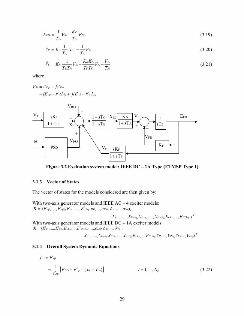
29
i
i
ii
i
i FDE
ER
EFD E
TKV
TE −=
1& (3.19)
i
i
i
i
ii RA
EA
AR VT
XT
KV 112 −=& (3.20)
i
ii
ii
iii
ii
ii
F
FR
FE
FER
FEFF
TVV
TTKKV
TTKV −−=
1& (3.21)
where
)IxEj()IxE(jVVV
iiiiii
ii
qqdddq
TdTqTi
′−′+′+′=+=
Figure 3.2 Excitation system model: IEEE DC – 1A Type (ETMSP Type 1)
3.1.3 Vector of States
The vector of states for the models considered are then given by: With two-axis generator models and IEEE AC – 4 exciter models:
TFDFDEEEE
Ng,Ng, , dd,qq
],...,E,E,.....,X,X,.....,X X
,δ,...,δ,...,ωωE,....,EE,....,E[
NgNgNg
NgNg
1221111
11 1211′′′′=X
With two-axis generator models and IEEE DC – 1A exciter models:
TFFRRFDFDEEEE
Ng,Ng, ,dd,qq
],...,VV,,...,V,V,...,E,E,.....,X,X,.....,X X
,δ,...,δ,...,ωωE,....,EE,....,E[
NgNgNgNgNg
NgNg
111221111
11 1211′′′′=X
3.1.4 Overall System Dynamic Equations
qiEf i ′= &1
[ ] gddqFDd
NixxEE iiii
i
,....,1)(10
=′−+′−′
=τ
(3.22)
F
F
sT1sK+
VT
VREF
XE1 –
+
PSS VPSS
+
B
C
sT1sT1
++
A
A
sT1K+
VR
+ EsT1
KE
F
F
sT1sK+
VF
–
ω
EFD
VFE
–
XE2
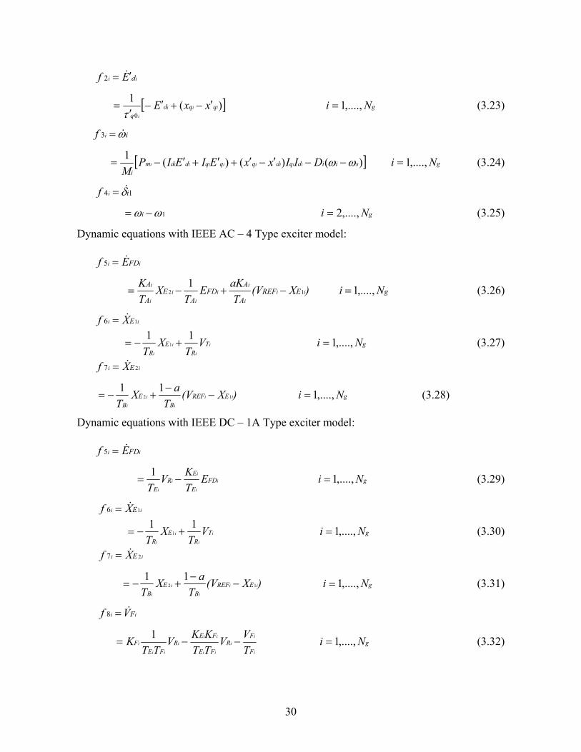
30
ii dEf & ′=2
[ ] gqqdq
NixxE iii
i
,....,1)(10
=′−+′−′
=τ
(3.23)
iif ω&=3
[ ] gsiidqdqqqddmi
NiDIIxxEIEIPM
iiiiiiiii ,....,1)()()(1=−−′−′+′+′−= ωω (3.24)
14 iif δ&=
gi Ni ,....,21 =−= ωω (3.25)
Dynamic equations with IEEE AC – 4 Type exciter model: ii FDEf &=5
gEREFA
AFD
AE
A
A Ni)X(VT
aKET
XTK
iii
ii
ii
i
i ,....,1112 =−+−= (3.26)
ii EXf 16 &=
gTR
ER
NiVT
XT
i
i
i
i
,....,1111 =+−= (3.27)
ii EXf 27 &=
gEREFB
EB
Ni)X(VT
aXT
ii
i
i
i
,....,11112 =−
−+−= (3.28)
Dynamic equations with IEEE DC – 1A Type exciter model: ii FDEf &=5
gFDE
ER
ENiE
TKV
Ti
i
ii
i
,....,11=−= (3.29)
ii EXf 16 &=
gTR
ER
NiVT
XT
i
i
i
i
,....,1111 =+−= (3.30)
ii EXf 27 &=
gEREFB
EB
Ni)X(VT
aXT
ii
i
i
i
,....,11112 =−
−+−= (3.31)
ii FVf &=8
gF
FR
FE
FER
FEF Ni
TVV
TTKKV
TTK
i
ii
ii
iii
ii
i ,....,11=−−= (3.32)

31
ii RVf &=8
gRA
EA
A NiVT
XT
K i
i
i
i
i ,....,1112 =−= (3.33)
In the above equations, VTi is the exciter input voltage such that,
0222 =′−′−′+′− )IxE()IxE(V iiiiii qqdddqTi The system is reduced to only the generator internal nodes and the load buses. A reference transformation [139] then yields the following expressions for the generator currents:
[ ] [ ]jijGB
Nj
jdijBGqijGB
Nj
jd VFEFEFI
ld
jj
g
i )()()(1
''
1δδδ −
=
=+−
=
=∑++∑= (3.34)
[ ] [ ]jijBGNj
jdijGBqijBG
Nj
jq VFEFEFI
ld
jj
g
i )()()(1
''
1δδδ +
=
=−+
=
=∑+−∑= (3.35)
i = 1, 2, …, Ng where
FG+B(δij) = Gij cos(δij) + Bij sin(δij) (3.36)
FB-G(δij) = Bij cos(δij) – Gij sin(δij) (3.37)
δij = δi – δj
The bus admittance matrix for the reduced network is YBus, with ijth element given by Yij∠ γij = Gij + jBij.
3.2 Algebraic Equations
The set of algebraic equations are the power balance equations at the load buses. These are derived in the following sub-sections.
3.2.1 Vector of Algebraic Variables
The vector of algebraic variables is made up of voltage magnitudes and voltage angles of load buses.
TNNNNNN ldggldgg VV ],....,,,.....,[ 11 +++ += δδY =[Vload δload]T
3.2.2 Load Model
Loads are modeled to be static voltage dependent. Each active power load is divided into two parts: controllable part and uncontrollable part.
pi
ii
pi
iiii
VVP
VVPUP i
UKi
KloadL
βα
⎟⎠⎞
⎜⎝⎛
⎟⎠⎞
⎜⎝⎛= +
0000 ; i = Ng+1, 2, 3, …., Ng+Nld (3.38)

32
where PK0i is the controllable part of the load, and PUK0i is the uncontrollable part of the load at bus i,
αpi and βpi are the voltage exponents that model the load corresponding to the controllable and uncontrollable parts of the load at bus i, and
Nld is the number of load buses.
The introduction of Uloadi in the above equation facilitates modeling the controllable part of the load at bus i as a system input as will be shown in the derivation of the linear model in the subsequent sections. Each reactive power load is also assumed to be static voltage dependent with voltage exponent βq.
qi
iii
iUKL
VVQQ
β
⎟⎠⎞
⎜⎝⎛=
00 ; i = Ng+1, 2, 3, …., Ng+Nld (3.39)
3.2.3 Power Balance Equations
The power balance equations at the load buses are as follows:
)Re( *00
00ii
iUK
iKloadL IV
VVP
VVPUP
pi
i
i
pi
i
iii =⎟⎠⎞
⎜⎝⎛
⎟⎠⎞
⎜⎝⎛= +
βα
; i = Ng+1, 2, 3, …., Ng+Nld (3.40)
)Im( *0
0ii
i
iUKL IV
VVQQ
qi
ii =⎟⎠⎞
⎜⎝⎛=
β
; i = Ng+1, 2, 3, …., Ng+Nld (3.41)
ii dqi jIII += i = Ng+1, 2, 3, …., Ng+Nld (3.42)
After reducing the system to generator internal nodes and load buses, reference transformation yields the following expressions for current injections at the load buses:
[ ]jj
g
i djijjijqjijjijNj
jd EBGEBGI ''
1))cos()sin(())sin()cos(( δδδδ +−−∑=
=
=
[ ]jjijjijNNj
NjVBG
ldg
g))sin()cos((
1δδ −∑+
+=
+= (3.43)
[ ]jj
g
i djijjijqjijjijNj
jq EGBEGBI ''
1))cos()sin(())sin()cos(( δδδδ −−+∑=
=
=
[ ]jjijjijNNj
NjVGB
ldg
g))sin()cos((
1δδ +∑+
+=
+= (3.44)

33
Substituting the above load current injections, (3.40) and (3.41) can be written in the following functional notation:
)Re( *00
00ii
iUK
iKloadL IV
VVP
VVPUP
pi
ii
pi
iiii =⎟
⎠⎞
⎜⎝⎛
⎟⎠⎞
⎜⎝⎛= +
βα
),...,,,....,,,...,,....,,....,( ,11,1,''
,''
11 ldldgggNgNgi NNNNNddqqp VVEEEEf δδδδ ++= (3.45)
)Im( *0
0ii
i
iUKL IV
VVQQ
qi
ii =⎟⎠⎞
⎜⎝⎛=
β
),...,,,....,,,...,,....,,....,( ,11,1,''
,''
11 ldldgggNgNg NNNNNddqqqi VVEEEEf δδδδ ++= (3.46)
ipg and iqg are non-linear functions of transient d-axis and q-axis voltages, load bus voltage
magnitudes and load bus voltage angles. Their forms are shown below:
[ ]
[ ] ⎥⎥⎥⎥
⎦
⎤
⎢⎢⎢⎢
⎣
⎡
−∑
++−−∑=
+=
+=
=
=
jjijjijNNj
Nj
djijjijqjijjijNj
jiip
VBG
EBGEBGVg
ldg
g
jj
g
i
))sin()cos((
))cos()sin(())sin()cos(()cos(
1
''
1
δδ
δδδδδ +
[ ]
[ ] ⎥⎥⎥⎥
⎦
⎤
⎢⎢⎢⎢
⎣
⎡
+∑
+−−+∑
+=
+=
=
=
jjijjijNNj
Nj
djijjijqjijjijNj
jii
VGB
EGBEGBV
ldg
g
jj
g
))sin()cos((
))cos()sin(())sin()cos(()sin(
1
''
1
δδ
δδδδδ (3.47)
[ ]
[ ]−
⎥⎥⎥⎥
⎦
⎤
⎢⎢⎢⎢
⎣
⎡
−∑
++−−∑=
+=
+=
=
=
jjijjijNNj
Nj
djijjijqjijjijNj
jiiq
VBG
EBGEBGVg
ldg
g
jj
g
i
))sin()cos((
))cos()sin(())sin()cos(()sin(
1
''
1
δδ
δδδδδ
[ ]
[ ] ⎥⎥⎥⎥
⎦
⎤
⎢⎢⎢⎢
⎣
⎡
+∑
+−−+∑
+=
+=
=
=
jjijjijNNj
Nj
djijjijqjijjijNj
jii
VGB
EGBEGBV
ldg
g
jj
g
))sin()cos((
))cos()sin(())sin()cos(()cos(
1
''
1
δδ
δδδδδ (3.48)
i = Ng+1, …., Ng+Nld
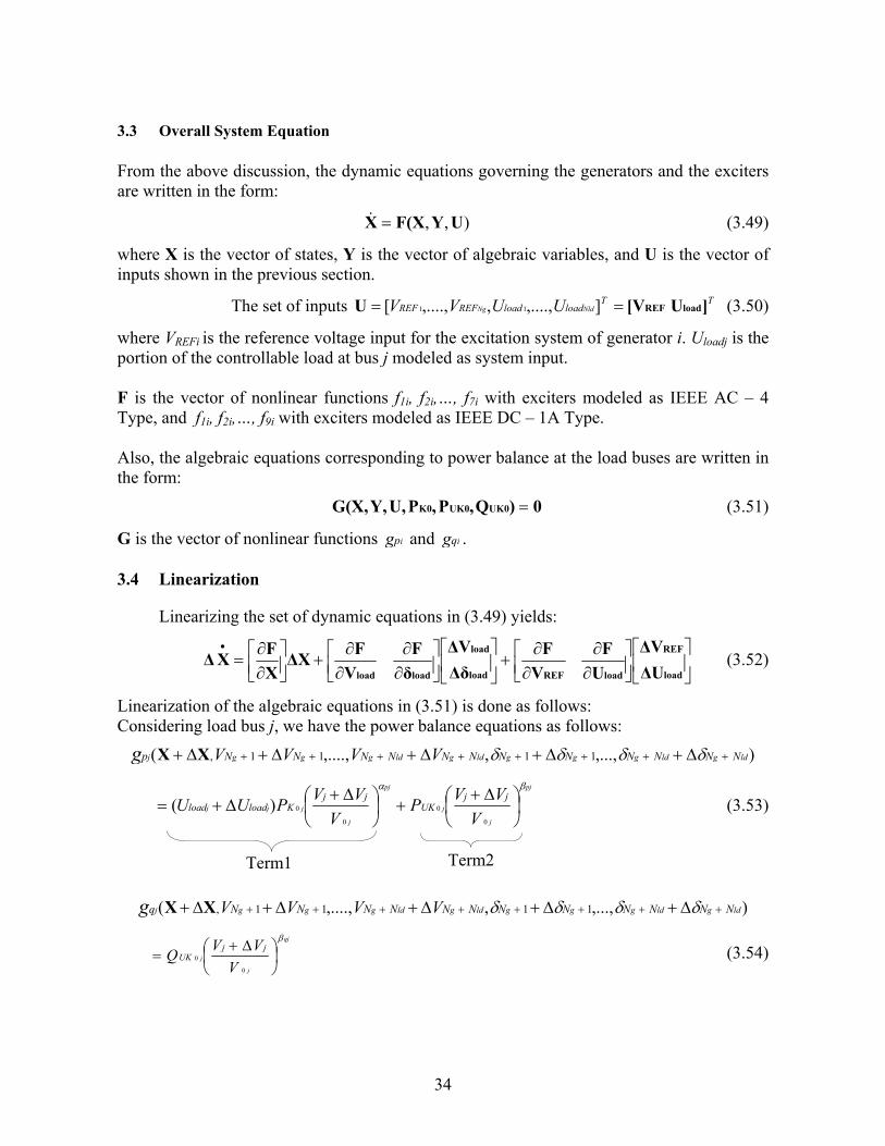
34
3.3 Overall System Equation From the above discussion, the dynamic equations governing the generators and the exciters are written in the form:
),, UYF(XX =& (3.49)
where X is the vector of states, Y is the vector of algebraic variables, and U is the vector of inputs shown in the previous section.
The set of inputs TTloadloadREFREF NldNg UUVV ]U[VU loadREF== ],....,,,....,[ 11 (3.50)
where VREFi is the reference voltage input for the excitation system of generator i. Uloadj is the portion of the controllable load at bus j modeled as system input. F is the vector of nonlinear functions f1i, f2i,…, f7i with exciters modeled as IEEE AC – 4 Type, and f1i, f2i,…, f9i with exciters modeled as IEEE DC – 1A Type. Also, the algebraic equations corresponding to power balance at the load buses are written in the form:
0)Q,P,PU,Y,G(X, UK0UK0K0 = (3.51)
G is the vector of nonlinear functions ipg and iqg .
3.4 Linearization
Linearizing the set of dynamic equations in (3.49) yields:
⎥⎦
⎤⎢⎣
⎡⎥⎦⎤
⎢⎣⎡
∂∂
∂∂
+⎥⎦
⎤⎢⎣
⎡⎥⎦⎤
⎢⎣⎡
∂∂
∂∂
+⎥⎦⎤
⎢⎣⎡∂∂
=•
load
REF
loadREFload
load
loadload ΔUΔV
UF
VF
ΔδΔV
δF
VFΔX
XFXΔ (3.52)
Linearization of the algebraic equations in (3.51) is done as follows: Considering load bus j, we have the power balance equations as follows:
),...,,,....,( 1111, ldgldgggldgldgggj NNNNNNNNNNNNp VVVVg ++++++++ Δ+Δ+Δ+Δ+Δ+ δδδδXX
pj
j
j
pj
j
jjj
VVVP
VVVPUU jj
UKjj
Kloadload
βα
⎟⎠⎞
⎜⎝⎛ Δ+
+⎟⎠⎞
⎜⎝⎛ Δ+
Δ+=0
0
0
0)( (3.53)
),...,,,....,( 1111, ldgldgggldgldgggj NNNNNNNNNNNNq VVVVg ++++++++ Δ+Δ+Δ+Δ+Δ+ δδδδXX qj
j
j
VVVQ jj
UK
β
⎟⎠⎞
⎜⎝⎛ Δ+
=0
0 (3.54)
Term1 Term2
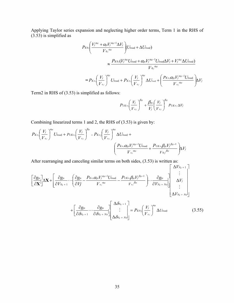
35
Applying Taylor series expansion and neglecting higher order terms, Term 1 in the RHS of (3.53) is simplified as
)(0
1
0 jjpj
j
pjpj
j loadloadjjpj
K UUV
VVVP Δ+⎟⎟⎠
⎞⎜⎜⎝
⎛ Δ+ −
α
αα α
pjj
jpj
jpj
jjpj
j
VUVVUVUVP loadjjloadjploadjK
α
ααα α0
10 )( Δ+Δ+
≈−
= jloadjpKj
Kloadj
K VV
UVUVVPU
VVP
pjj
jpj
jjloadj
pj
j
jj
pj
j
jP
Δ⎟⎟⎠
⎞⎜⎜⎝
⎛+Δ⎟
⎠⎞
⎜⎝⎛+⎟
⎠⎞
⎜⎝⎛ −
α
ααα α0
0
0
0
0
0
1
Term2 in RHS of (3.53) is simplified as follows:
jUKj
j
pjUK VP j
pj
j
jpj
j
j
VV
VV
PV
Δ⎟⎠⎞
⎜⎝⎛
⎟⎠⎞
⎜⎝⎛ + 0
00
0
ββ β
Combining linearized terms 1 and 2, the RHS of (3.53) is given by:
jj
jpUKloadjpK
loadj
jKj
UKloadj
K
VVPV
UVP
UVVP
VVU
VVP
pj
pjjj
pjj
jpj
jj
j
pj
j
pj
j
jj
pj
j
j
V
P
Δ⎟⎟⎠
⎞⎜⎜⎝
⎛+
+Δ⎟⎠⎞
⎜⎝⎛
⎟⎠⎞
⎜⎝⎛+⎟
⎠⎞
⎜⎝⎛
−−
+
β
β
α
α
αβα
βα0
110
0
0
0
0
0
0
0
0
After rearranging and canceling similar terms on both sides, (3.53) is written as:
⎥⎥⎥⎥⎥⎥
⎦
⎤
⎢⎢⎢⎢⎢⎢
⎣
⎡
⎥⎥⎦
⎤
⎢⎢⎣
⎡
∂∂
⎜⎜⎝
⎛⎟⎟⎠
⎞−−
∂∂
∂∂
+⎥⎦⎤
⎢⎣⎡∂∂
+
+
+
−−
+
ldg
g
ldg
j
pjj
pjjj
pjj
jpj
jjj
g
jj
NN
j
N
NN
pjpUKloadjpKp
N
pp
V
V
V
VgVP
VUVP
Vjg
Vgg
V
Δ
Δ
Δ
Δ
1
11
1 0
0
0
0
M
M
LL β
β
α
α βαXX
j
pj
j
ldg
g
ldg
j
g
jload
jjK
NN
N
NN
p
N
pU
VVPgg Δ
Δ
Δ
0
0
1
1
α
δ
δ
δδ⎟⎠⎞
⎜⎝⎛=
⎥⎥⎥
⎦
⎤
⎢⎢⎢
⎣
⎡
⎥⎦⎤
∂∂
⎢⎣⎡∂∂
++
+
++ML (3.55)

36
⎥⎥⎥⎥⎥⎥
⎦
⎤
⎢⎢⎢⎢⎢⎢
⎣
⎡
⎥⎥⎦
⎤
⎢⎢⎣
⎡
∂∂
⎜⎜⎝
⎛⎟⎟⎠
⎞−
∂∂
∂∂
+⎥⎦⎤
⎢⎣⎡∂∂
+
+
+
−
+
ldg
g
ldg
jp
jj
g
jj
NN
j
N
NN
q
pj
jpUKq
N
V
V
V
Vg
VVQ
Vjg
Vgg
Δ
Δ
Δ
Δ
1
1
1 0
0
M
M
LL β
ββXX
0Δ
Δ 1
1=
⎥⎥⎥
⎦
⎤
⎢⎢⎢
⎣
⎡
⎥⎦⎤
∂∂
⎢⎣⎡∂∂
++
+
++ldg
g
ldg
j
g
j
NN
N
NN
q
N
q gg
δ
δ
δδML (3.56)
Considering all load buses, the linearized active power balance equation is then given by:
+
⎥⎥⎥⎥⎥⎥
⎦
⎤
⎢⎢⎢⎢⎢⎢
⎣
⎡
Δ
Δ
Δ
⎥⎥⎥⎥⎥⎥⎥⎥
⎦
⎤
⎢⎢⎢⎢⎢⎢⎢⎢
⎣
⎡
−∂∂
∂∂
∂∂
+∂∂
−∂∂
∂∂
+∂∂
∂∂
−∂∂
+Δ⎥⎦⎤
⎢⎣⎡∂∂
+
+
++
+
+
+
+++
++
+
+
ld
NldNgld
NldNgNldNgNldNg
ldg
jj
jj
ldg
NgNg
Ng
Ng
NNg
j
Ng
pNNg
p
j
p
Ng
p
NN
pp
j
p
Ng
p
NN
p
j
pp
Ng
p
V
V
V
TVg
Vg
Vg
VgT
Vg
Vg
Vg
Vg
TVg
M
M
LL
MMMMM
LL
MMMMM
LL1
1
1
1
11
1
1
XXgp
=
⎥⎥⎥⎥⎥⎥
⎦
⎤
⎢⎢⎢⎢⎢⎢
⎣
⎡
Δ
Δ
Δ
⎥⎥⎥⎥⎥⎥⎥⎥
⎦
⎤
⎢⎢⎢⎢⎢⎢⎢⎢
⎣
⎡
+∂∂
∂∂
∂∂
+∂∂
∂∂
∂∂
+∂∂
∂∂
∂∂
+
+
+
+
+
+
+++
+++
ld
ldg
NldNgNldNgNldNg
ldg
jjj
ldg
NgNg
g
Ng
NNg
j
Ng
NN
p
j
p
Ng
p
NN
p
j
p
Ng
p
NN
p
j
p
N
p
ggg
ggg
ggg
δ
δ
δ
δδδ
δδδ
δδδ
M
M
LL
MMMMM
LL
MMMMM
LL1
1
1
1
111
⎥⎥⎥⎥⎥⎥⎥⎥⎥⎥⎥
⎦
⎤
⎢⎢⎢⎢⎢⎢⎢⎢⎢⎢⎢
⎣
⎡
Δ
Δ
ΔΔ
Δ
⎥⎥⎥⎥⎥⎥⎥⎥⎥
⎦
⎤
⎢⎢⎢⎢⎢⎢⎢⎢⎢
⎣
⎡
⎟⎠⎞
⎜⎝⎛
⎟⎠⎞
⎜⎝⎛
⎟⎠⎞
⎜⎝⎛
+
+
+
+
+
+
++
+
+
++
NldNg
j
Ng
NldNg
Ng
NldNg
NldNg
NldNgNldNg
j
j
j
Ng
Ng
gNg
load
load
load
REF
REF
K
pj
K
pN
K
U
U
UV
V
VVP
VVP
VVP
pM
M
M
LLL
MMMMMMMM
L
MMMMMMMM
LLL
1
11
1
1
00
00
0
10
0000
000000
0000
α
α
α
(3.57)
Bpv
Bpδ
RHp

37
where
⎜⎜⎝
⎛⎟⎟⎠
⎞+=
−−
pjj
pjjj
pjj
jpj
jjj
VV
VUVPT jpUKloadjpK
pP
β
β
α
α βα0
0
0
011
(3.58)
(3.57) is concisely written as
[ ] [ ] ⎥⎦
⎤⎢⎣
⎡=⎥
⎦
⎤⎢⎣
⎡+⎥⎦
⎤⎢⎣⎡∂∂
load
REF
load
loadp
ΔUΔV
RHp0ΔδΔV
BpδBpvΔXXg (3.59)
A similar equation results for the linearized reactive power balance equation:
[ ] 0δV
BqδBqvΔXXg
load
loadq=⎥
⎦
⎤⎢⎣
⎡ΔΔ
+⎥⎦⎤
⎢⎣⎡∂∂ (3.60)
From (3.59) and (3.60),
⎥⎦
⎤⎢⎣
⎡⎥⎦
⎤⎢⎣
⎡⎥⎦
⎤⎢⎣
⎡+
⎥⎥⎥
⎦
⎤
⎢⎢⎢
⎣
⎡
∂∂∂∂
⎥⎦
⎤⎢⎣
⎡−=⎥
⎦
⎤⎢⎣
⎡−−
load
REF1
q
p1
load
load
ΔUΔV
00RHp0
BqδBqvBpδBpv
ΔΧ
XgXg
BqδBqvBpδBpv
ΔδΔV
(3.61)
Substituting for [ΔVload Δδload]T from (3.61) in (3.52) yields
+Δ
⎢⎢⎢⎢
⎣
⎡
⎥⎥⎥⎥
⎦
⎤
⎥⎥⎥
⎦
⎤
⎢⎢⎢
⎣
⎡
∂∂∂∂
⎥⎦
⎤⎢⎣
⎡⎥⎦⎤
⎢⎣⎡
∂∂
∂∂
−⎥⎦⎤
⎢⎣⎡∂∂
=−
Χ
XgXg
BqδBqvBpδBpv
δF
VF
XFXΔ
q
p
loadload
1&
ΔU00
RHp0BqδBqvBpδBpv
UF
VF
loadREF⎢⎢⎣
⎡
⎥⎥⎦
⎤⎥⎦
⎤⎢⎣
⎡⎥⎦
⎤⎢⎣
⎡+⎥⎦
⎤⎢⎣⎡
∂∂
∂∂
−1
(3.62)
UΔBXAΔ +=
where
⎢⎢⎢⎢
⎣
⎡
⎥⎥⎥⎥
⎦
⎤
⎥⎥⎥
⎦
⎤
⎢⎢⎢
⎣
⎡
∂∂∂∂
⎥⎦
⎤⎢⎣
⎡⎥⎦⎤
⎢⎣⎡
∂∂
∂∂
−⎥⎦⎤
⎢⎣⎡∂∂
=−
XgXg
BqδBqvBpδBpv
δF
VF
XFA
q
p
loadload
1
(3.63)
⎢⎢
⎣
⎡
⎥⎥⎦
⎤⎥⎦
⎤⎢⎣
⎡⎥⎦
⎤⎢⎣
⎡+⎥⎦
⎤⎢⎣⎡
∂∂
∂∂
=−
00RHp0
BqδBqvBpδBpv
UF
VFB
1
loadREF (3.64)

38
4. Structured Singular Value Based Performance Analysis Framework
This section begins with a brief historical overview of Structured Singular Value (SSV) theory followed by a summary of uncertainty representation, structured singular value definition, linear fractional transformation, fundamental theorems and results related to SSV theory, the concept of skewed – μ and its relevance to robust performance analysis. The characterization of uncertainty in the state-space model of the power system, the selection of error signal for characterizing performance and the development of the framework for robust performance analysis using the structured singular value theory are then presented in detail.
4.1 Structured Singular Value Theory – A Brief Historical Overview
The concept of Structured Singular Value (μ) was first introduced as Small Mu theorem by John Doyle in 1982 [119] to determine the stability of a system that is subject to structured perturbations (or uncertainties). The origins of μ – theory are based on small-gain theory developed by George Zames in 1966 [120] to analyze the stability of MIMO systems in the presence of unstructured uncertainties. Unstructured uncertainties are those that are bounded in some sense but do not have any special structure. The small-gain theorem is actually a generalization of the classical Nyquist stability criterion, which was developed in 1932, as a graphical method for determining the stability of linear SISO systems. The small gain theorem provided an exact robust stability test with respect to unstructured dynamic perturbations. This work further introduced the use of singular values as an important tool in robust control. It is, however, conservative (i.e., sufficient but not necessary) when the uncertainty in the system has some structure. Several researchers looked at the problem of exploiting the uncertainty structure to reduce conservatism, and Doyle introduced complex μ as a systematic means of dealing with such problems. This work also introduced the use of both upper and lower bounds for μ, and stressed the need for viable methods of computing these bounds. The complex μ theory was extended considerably by a number of researchers. An important element of this research was the emphasis on efficient computation of the bounds for μ, rather than the exact computation of μ. Subsequently, Doyle proposed D-K iteration [121] for complex μ synthesis. The theoretical research further led to the release of μ – Tools toolbox by Balas et al [143], a commercially available software package with the algorithms necessary to implement complex μ analysis and synthesis techniques. In recent years, μ tools and techniques have steadily matured to a level suitable for application to large engineering problems.

39
4.2 Uncertainty Representation
The various sources of uncertainty in any mathematical model of a physical system may be broadly classified into the following two types:
1. Parametric uncertainty: In this category, the structure of the model (including the order) is known, but there exist some parameters that are uncertain.
2. Model uncertainty: Here the model is erroneous because of missing dynamics, usually at high frequencies, either through deliberate neglect or because of a lack of understanding of the physical process. Any model of a real system will contain this source of uncertainty.
Parametric uncertainty will be quantified by assuming that each uncertain parameter, α, is bounded within some region [αmin, αmax]. That is, we have parameter sets of the following form:
( )Δ+= ααα r1p (4.1)
where α is the mean parameter value, αr = (αmax– αmin)/( αmax+αmin) is the relative uncertainty in the parameter, Δ is any real scalar satisfying 1Δ ≤ . Frequency domain is well suited for representation of model uncertainties. These are complex perturbations which are normalized such that 1≤Δ
∞.
In this research, we will use the state-space model developed in the previous section to model the parametric uncertainty in power systems. Parametric uncertainty encompasses the uncertainty corresponding to physical parameters of the model as well as that corresponding to operating condition changes. The uncertainty in operating conditions modeled in this research includes uncertainty in load levels, generation levels as well as power exchanges. Model uncertainty will be used to characterize the robust performance analysis problem as an equivalent robust stability analysis problem. This is done through augmenting the parametric uncertainty block with a full-block complex uncertainty. This is essentially the robust performance theorem (Theorem 4.2) stated and explained in Section 4.6.
4.3 Structured Singular Value μ
The definition of μ for a general complex matrix M comes from the task of finding the smallest structured uncertainty Δ (measured in terms of the maximum singular value of Δ,
)(Δσ ), which makes det(I-MΔ)=0, so μ is independent on the underlying block structure of the uncertainty. More precisely, suppose we have a complex matrix nxnM C∈ and three non-negative integers mr, mc, and mC (with m:= mr+ mc+ mC ≤ n), which specify the number of uncertainty blocks

40
of repeated real scalars, repeated complex scalars, and full complex blocks, respectively. Then the block structure K(mr, mc, mC) is an m-tuple of positive integers:
),...,,,...,,,...,( 111 mmmmmmm kkkkkkcrcrrr ++++=κ (4.2)
This m-tuple specifies the dimensions of the perturbation blocks. And we require nkmi i =∑ =1
in order that these dimensions are compatible with M. This determines the following set of allowable uncertainty: ,,...,,,...,diag(block :
11 11
cmrmcrmrmr kcmk
ck
rmkrκ IIIIX
++== δδδδΔ
Δ,,:)Δ,...,Δ1icmrmicmrm
C
kCi
ci
ri
Cm
C ++×++∈∈∈ CCR δδ (4.3)
Then )(Mκμ , the SSV of matrix M with respect to a block structure ),,( Ccr mmmκ , is defined as follows:
1
Δ0Δ)det( :Δ)(min:)(
−
∈⎟⎠
⎞⎜⎝
⎛== I-MM
Xσμ
κκ (4.4)
with )(Mκμ =0 if det(I–MΔ) ≠ 0 for all Δ∈ κX .
Note that the block structure of κX in (4.3) is sufficiently general to allow (any combination of) repeated real scalars, repeated complex scalars, and full complex blocks. There are two special cases in which the definition of μ can be simplified:
1. Δ is a repeated real scalar block, i.e., mr=1 and mc = mC = 0, we have )(Mκμ =ρR(M)
where of eigenvalue real a is λ:λmax:)( MMR =ρ , with ρR(M)=0 if M has no real eigenvalues. Thus μ is the real spectral radius of M.
2. Δ is a full complex block (unstructured uncertainty), i.e., mr = mc = 0 and mC = 1, we have
)()( MM σμκ = For a general type of uncertainty Δ∈ κX , the following holds:
ρR(M) ≤ )(Mκμ ≤ )(Mσ (4.5)
so μ can be viewed as a generalization of both the real spectral radius and the maximal singular value. From the definition of μ in (4.4), it is not obvious how the value of μ may be computed. In fact, the exact calculation of μ is generally very difficult [122]. Equation (4.5) provides the lower and upper bounds for μ, however, both the bounds are too crude since the gap between them can be arbitrarily large in some cases. In order to reduce this gap, the following sets of scaling matrices are defined:

41
[ ]
0,0
:),...,,,...,diag(block :
ΔΔ,1,1,1:Δ:
*
11
**
1
RC ∈<∈=<
=
==−∈∈=
×
+ ++
++
ikk
ii
kmkmmκ
kCi
Ci
ci
ci
riκκ
dDD
IdIdDDD
IXQ
ii
mCcmrmcr
icmrmδδδ
With these scaling matrices, the lower bound and upper bound can be refined as
)(inf)()(max 1−
∈∈≤≤ DMDMQM
DDRQQσμρ
κκκ (4.6)
It has been proved in [119] that the first inequality in (4.6) is actually an equality. However, the function ρ(QM) is not convex in κQQ∈ and therefore it is not guaranteed to find the
global maximum. The practical computation uses a power iteration algorithm to find a local maximum and thus obtains a lower bound for μ. On the other hand, the calculation of upper bound from (4.6) is a convex minimization problem for the maximal singular value, so all local maxima are global and hence this bound is computationally attractive. The commercially available MATLAB toolbox, μ – Tools, is used to compute μ upper and lower bounds.
4.4 Linear Fractional Transformation
Linear Fractional Transformations (LFTs) offer a useful way to standardize block diagrams to perform analysis and design for robust control. The basic principle behind the application of LFTs in robust control is the separation of the uncertain (or varying) part of the system from the nominal system. Consider a matrix nxnN C∈ partitioned as
⎥⎦
⎤⎢⎣
⎡=
2221
1211
NNNN
N (4.7)
with 1111
xnnN C∈ and 2222
xnnN C∈ and n1+n2 = n. Suppose we have block structures 1κX
and 2κX defined as follows:
Δ:Δ
Δ:Δ
222
111
22
11
nnκ
nnκ
X
X
×
×
∈=
∈=
C
C
then the block structure of κX defined as
Δ,Δ:)Δ,diag(Δblock Δ:21 2121 κκκ XXX ∈∈== (4.8)
is compatible with N.

42
4.4.1 Well-posedness of LFTs
Given any11Δ κX∈ , the LFT Fu(N,Δ1) is said to be well-posed if and only if there exists a
unique solution to the loop equations shown in Figure 4.1, namely,
Figure 4.1 Upper linear fractional transformation
wz
dNzNedNzNw
1
2221
1211
Δ=+=+=
Alternatively, Fu(N,Δ1) is well-posed if and only if ( )111Δ1NIn − is invertible.
4.4.2 Definition
When the LFT is well-posed, it is defined to be a unique mapping from d to e, i.e., the vectors e and d satisfy e = Fu(N, Δ1)d where
121
111121221 )Δ(Δ:)Δ,(1
NNINNNF nu−−+= (4.9)
In this definition, the feedback is assumed to be closed around the top inputs and outputs, and hence we obtain an upper LFT (denoted by Fu). A lower LFT can analogously be as follows defined when feedback is closed around the lower inputs and outputs:
211
222212112 )Δ(Δ:)Δ,(2
NNINNNF nl−−+= (4.10)
4.4.3 Basic Principle
The basic principle at work here in writing a matrix LFT is often referred to as “pulling out the Δ’s”. This is illustrated below with Figure 4.2 and Figure 4.3. Consider a structure with four substructures interconnected in some known way, as shown in Figure 4.2. This diagram can be redrawn as a standard one via “pulling out the Δ’s” in Figure 4.3. Now, the matrix N of the LFT in (4.9) can be obtained by computing the corresponding transfer matrix P in the shadowed box in Figure 4.3 and then evaluating the lower LFT
Δ1
Ne
w z
d
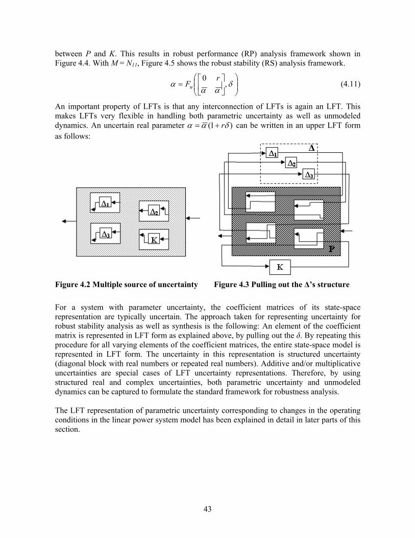
43
between P and K. This results in robust performance (RP) analysis framework shown in Figure 4.4. With M = N11, Figure 4.5 shows the robust stability (RS) analysis framework.
⎟⎟⎠
⎞⎜⎜⎝
⎛⎥⎦
⎤⎢⎣
⎡= δ
ααα ,
0 rFu (4.11)
An important property of LFTs is that any interconnection of LFTs is again an LFT. This makes LFTs very flexible in handling both parametric uncertainty as well as unmodeled dynamics. An uncertain real parameter )1( δαα r+= can be written in an upper LFT form as follows:
Figure 4.2 Multiple source of uncertainty Figure 4.3 Pulling out the Δ’s structure For a system with parameter uncertainty, the coefficient matrices of its state-space representation are typically uncertain. The approach taken for representing uncertainty for robust stability analysis as well as synthesis is the following: An element of the coefficient matrix is represented in LFT form as explained above, by pulling out the δ. By repeating this procedure for all varying elements of the coefficient matrices, the entire state-space model is represented in LFT form. The uncertainty in this representation is structured uncertainty (diagonal block with real numbers or repeated real numbers). Additive and/or multiplicative uncertainties are special cases of LFT uncertainty representations. Therefore, by using structured real and complex uncertainties, both parametric uncertainty and unmodeled dynamics can be captured to formulate the standard framework for robustness analysis. The LFT representation of parametric uncertainty corresponding to changes in the operating conditions in the linear power system model has been explained in detail in later parts of this section.

44
Figure 4.4 RP analysis framework Figure 4.5 RS analysis framework
4.5 Robust Stability
The most well-known use of μ as a robustness analysis tool is in the frequency domain. In the robust stability analysis framework shown in Figure 4.5, let M be a stable, real, rational, MIMO transfer function of a linear system. With only real-parametric uncertainties considered in robust stability analysis, the general uncertainty structure in (4.3) can be simplified to
:,...,:11 RΔ ∈= r
ikrSk
rs S
II δδδ (4.12)
where nkSi i =∑ =1 .
The following theorem addresses the robust stability of linear uncertain systems: Theorem 4.1 (Robust Stability [122]) Suppose M(s) is a nominally stable system (otherwise,
the problem is trivial), then for all Δ in ΔS satisfying β
σ 1Δ)( ≤ , the perturbed closed-loop
system shown in Figure 4.5 is well posed and internally stable if and only if
βωμ <∈
))((sup jMS
RωΔ (4.13)
The most important implication of this theorem is that we can assess the robustness properties of the closed-loop system through a frequency domain evaluation of μ. The peak value of the μ plot of the frequency response determines the size of perturbations that the closed loop is robustly stable against. As mentioned earlier, the μ – toolbox software does not compute μ exactly, but bounds it from above and below by several optimization steps. Hence the conclusion can be restated in terms of upper and lower bounds of μ. Let βu and βl be the upper and lower bounds respectively, then
• For all uncertainty matrices Δ in Δs satisfying uβ
σ 1Δ)( ≤ , the closed-loop system is
stable.
Δ
N e
w z
d
Δ
Mw z

45
• There is a particular uncertainty matrix Δ in Δs satisfying lβ
σ 1Δ)( = that causes
instability.
4.6 Robust Performance
Often, stability is the minimum requirement of a closed-loop system that must be robust to perturbations. Typically, there are exogenous disturbances acting on the system that result in tracking and regulation errors. Under perturbation, the effect that these disturbances have on error signals can greatly increase. In most cases, long before the onset of instability, the closed-loop performance will degrade to a point that would be unacceptable. This motivates the need for robust performance test. The robust performance analysis framework is shown in Figure 4.4 above. The transfer function between the exogenous disturbance vector d and the error signal vector e is obtained by evaluating the upper LFT between N and Δ, Fu(N,Δ). The robust performance requirement is characterized by the H∞ norm of Fu(N,Δ). The H∞ norm of a transfer function T is defined as ))((max ωσ
ωjTT
R∈∞= .
The robust performance condition could be checked by computing μ(N) with a modified uncertainty characterization as stated in the following theorem.
Theorem 4.2 (Robust performance [122]) Suppose M(s) is a nominally stable system
(otherwise, the problem is trivial),then for all Δ in ΔS satisfying β
σ 1Δ)( ≤ , the perturbed
closed-loop system shown in Figure 4.5 is well posed and internally stable, and β<
∞Δ),(NFu if and only if
βωμ <∈
))((sup jNP
RωΔ (4.14)
where ⎪⎭
⎪⎬⎫
⎪⎩
⎪⎨⎧
∈∈⎥⎦
⎤⎢⎣
⎡= × ed nn
pSp
P CΔΔ Δ,Δ:Δ00Δ
: (4.15)
As a special case, for normalized Δ (β=1), the closed-loop system is said to achieve robust performance if and only if 1))((sup <
∈ωμ jN
PRω
Δ .
Essentially, this theorem states that a robust performance problem is equivalent to a robust stability problem with an augmented uncertainty block, diag(Δ, Δp), as illustrated in Figure 4.6 below. Δp is a full complex matrix of dimension ed nn × where nd and ne are the dimensions of d and e respectively.

46
Figure 4.6 RP analysis as a special case of structured RS analysis
In this report, robust performance analysis is performed in two fundamentally different ways. As can be seen from Theorem 4.2 and Figure 4.6, μ for robust performance (performance μ) is evaluated with respect to the augmented uncertainty structure. There are two factors that influence the value of performance μ – the performance specification and the uncertainty – resulting in two different approaches to robust performance analysis.
a. For a given performance specification, it is possible to determine the worst-case uncertainty size that results in the performance μ being unity.
b. Alternatively, for a given uncertainty, it is possible to evaluate the worst-case performance.
Both these approaches have been applied in this report to determine the amount of load modulation to be performed to satisfy the desired damping performance specifications. The details are presented in section 5.
4.7 Skewed μ
A value of μ = 1.1 for robust stability means that all the uncertainty blocks must be decreased in magnitude by a factor 1.1 in order to guarantee stability. However, if some of the uncertainty blocks are fixed, how large can one particular source of uncertainty be that results in stability? The answer to this question is given by skewed – μ (μs). μs(M) can be viewed as a generalization of μ(M). For example, let Δ = diagΔ1, Δ2 and let Δ1 be fixed with 1Δ1 ≤ . The objective is to find how large Δ2 can be before we get instability. The solution is to select
⎥⎦
⎤⎢⎣
⎡=
IkI
Km
m 00
(4.16)
and look at each frequency for the smallest value of km which makes det(I–KmMΔ)=0, and we have that skewed – μ is
ms kM 1:)( =μ (4.17)
Δ
N e
w z
d
Δ
Ne
w z
d
Δp
47
In order to compute skewed – μ, the part of the perturbation that must be maintained constant must be defined. μs(M) is always further from 1 than μ(M) is, i.e., μs(M) ≥ μ(M) for μ(M) > 1 and μs(M) ≤ μ(M) for μ(M) < 1. For μ(M) = 1, μs(M) = μ(M). In practice, μs can be computed by iterating on km until μ(KmM) = 1 where Km may be as in (4.16). This iteration is straightforward since μ increases uniformly with km. Both the approaches to robust performance analysis mentioned above are skewed – μ based approaches. This is because a part of the perturbation, either the performance part or the parametric part, is kept constant in both. An important implication is that robust performance analysis, unlike robust stability analysis, is iterative. This is explained in more detail in the next section.
4.8 SSV – Based Framework for Robust Performance Analysis
4.8.1 Characterization of Parametric Uncertainty in the Linearized Model
The following are the different sources of parametric uncertainty considered in this research: uncertainty in controllable load levels at various load buses, uncertainty in generation levels. These two uncertainties result in uncertainties in power exchanges between different areas of the system. As discussed earlier, parametric uncertainties translate into uncertainties in the elements of the coefficient matrices of the state-space model. In [132], a framework is developed to capture the uncertainty in each varying element of the A-matrix of the state-space model and represent the uncertainty in the entire matrix in an LFT form. The uncertainty thus represented has a block diagonal structure. This approach for uncertainty characterization forms the basis of the framework developed in this research for robust performance analysis and is explained in detail in the following. Routine analysis of the linear model identifies that for an n-machine system with the dynamic models mentioned in Section 3, (4n) x (3n-1) elements of the A-matrix vary with the operating conditions (controllable load levels, generation levels) or model parameters. For each machine, the changing elements correspond to iEdiqi XEE 1
'' ,,, &&&& ΔΔΔΔ ω rows and 1
'' ,, idiqi EE δΔΔ columns. Each coefficient aij of the A-matrix that changes with the operating condition stays within a certain interval: [ maxmin
ijij aa − ]. The A-matrix elements that change with the operating conditions are not mutually independent. Instead they depend on the set of independent parameters p1,p2,…,pm, that is, the controllable loads at the buses and/or the generation, which take values in the known range [ maxmin
kk pp − ] for k=1,2,…m. Thus the varying A-matrix elements can be expressed as: ),...,,( 21 mijij pppfa = . Since the A-matrix elements for a given operating condition are obtained only after the power flow equations are solved, the functions fij cannot in general be calculated explicitly – although the
),...,,( 21 mij pppf value itself is computable for a given set of parameters mppp ,...,, 21 .

48
The dependence of the aij coefficients on the parameters mppp ,...,, 21 is captured by approximating functions fij. A linear approximation has been found to be adequate in representing each varying element of the A-matrix. Using a linear approximation for the varying elements of A-matrix, the entire A-matrix is written in a Linear Fractional Transformation (LFT) form. The approximation procedure essentially consists of setting up an over determined system of linear equations for the coefficients at various points on a grid of controllable loads and/or generation at different buses. These equations are then solved using a least square minimization approach. Assuming without loss of generality that there are two controllable loads that are uncertain, each coefficient of the A-matrix which depends on the uncertain controllable load at the buses selected for control is expressed by the following polynomial approximation:
21 210papaaa ijijijij ′+′+′= (4.18)
where pkmin ≤ pk ≤ pk
max. k=1, 2. It is desirable to normalize the range of variation of pk in a way to make the allowable range for each pk in the interval [-1,1]. This is done by defining:
kkkkk
kppppp δ
22
minmaxmaxmin−
++
= (4.19)
where -1≤ kδ ≤1; k = 1,2. Substituting the above expression yields
21 210 δδ ijijijij aaaa ++= (4.20)
Using the above equation, the dependence of the A-matrix elements on the parameters δ1 and δ2 can be expressed. The dependence of the A-matrix on the parameters δ1 and δ2 can be written as:
A21T
A0 RIAIALAA )]()([ 21 δδ ++= (4.21)
Similar to the A-matrix, the dependence of B-matrix on δ1 and δ2 could be expressed as follows:
B2211T
B0 RIBIBLBB )]()([ δδ ++= (4.22)

49
Figure 4.7 LFT representation of parametric uncertainty in state-space model
Matrices LA, RA, LB and RB consist of 0’s and 1’s and they allow efficient representation of the dependence of A-matrix and B-matrix on δ1 and δ2 respectively. RAX gives the vector of state variables whose corresponding columns in the A-matrix change with the change of the operating conditions, as suggested in [132]. Similarly LA matrix is defined such that XLA & gives the vector of state variables whose corresponding rows in the A-matrix change with change of operating conditions. The idea behind RA and LA has been extended here to RB and LB, with respect to the vector of inputs U. Thus RBU gives the vector of state variables whose corresponding columns in the B-matrix change with the change of operating conditions. LBU gives the vector of state variables whose corresponding rows in the B-matrix change with the operating conditions. Using these matrices, the dependence of A and B matrices on δ1 and δ2 is represented in a Linear Fractional Transformation (LFT) form as shown in Figure 4.7.
ZB1 WB1
RA
∑
LATX&
A0∑
B0∑
∑
LBT
δ1I
δ2I
δ2I
δ1I
A2 A1
RB
B1 B2
X
⎥⎦⎤
⎢⎣⎡UloadVREF
ZB2
WA1
WA2
ZA1
ZA2
WB2
P0

50
4.8.2 Characterization of Performance through the Choice of Error Signals
Besides the uncertainty characterization, the other important component of the robust performance analysis framework is performance characterization. This is accomplished through carefully selected error signals for the linear model that are representative of the performance desired. The error signals thus selected need to be appropriately weighted in order to take care of different objectives over a range of frequency. The weighted error signals together with the uncertainty characterization are then cast into the form suitable for robust performance analysis using the structured singular value theory. The error signal chosen for the framework developed here is the inertia weighted average of the angular speeds of generators that participate in the critical oscillatory modes under consideration in the center of inertia frame of reference. Inter-area oscillatory modes, as explained in Section 1, are characterized by significant participation by a number of generators. The participation factors as well as the mode shapes of different generators could change over the uncertain operating range. It is necessary to validate the choice of the speeds to be included in the error signal through time-domain simulation. SIMGUI tool available in Matlab μ – toolbox is made use of in simulation of error signal responses. SIMGUI is a time-domain simulation package for uncertain linear MIMO control systems expressed in the LFT form. It could be used to perform time-domain simulation of the nominal plant as well as the uncertain system for varying sizes of the uncertainty. It plots the error signal responses excited as a result of the disturbance input in the LFT generalized plant model. For each modification in the error signal, the corresponding responses could be plotted for range of uncertainties and it provides an effective tool to verify the choice of the error signal.
4.8.2.1 Illustration of Error Signal Construction Using SIMGUI
4.8.2.1.1. Nordic System
The application of SIMGUI tool for error signal selection is illustrated here with an example for the Nordic system augmented with distribution sub-system. Table 4.1 shows some of the oscillatory modes observed in this system characterized by participation from multiple generators.

51
Table 4.1 Oscillatory modes observed in Nordic system and participation of different generators
S.No. Mode frequency in Hz
Participating Generators
1 0.62 6, 9, 10 2 0.77 8, 19 3 1.11 7, 18, 20 4 1.14 7, 20 5 1.06 1, 7, 12, 14, 15, 20 6 0.84 8, 19 7 0.41 1, 6, 9, 8, 10, 12,
Mode 7 with a frequency of around 0.41 Hz has been observed to be the least-damped mode. It is also the one that rapidly changes with operating conditions making it a critical oscillatory mode. This mode has been selected for illustrating the choice of error signals. Table 4.2 shows the magnitude of participation factors of the speed (ω) and angle (δ) states of different generators for this mode for the nominal operating point. The procedure adopted in constructing the error signal using SIMGUI is described below:
Table 4.2 Calculated participation factors of speed and angle states for Mode # 7
Generator State Participation factor in %
12 ω 20.52 6 δ 13.39 9 δ 12.03 10 δ 10.37 9 ω 9.27
10 ω 8.43 6 ω 8.04
12 δ 7.16 8 δ 5.92 1 ω 5.41 8 δ 4.78 7 δ 4.12 7 ω 3.05
Starting with the angular speed corresponding to the machine with the highest participation in the inter-area mode, inertia weighted angular speeds corresponding to different machines are added to the error signal with proper signs (as indicated by the mode shapes) in the descending order of participation factor magnitudes. At each stage the linear system corresponding to both the nominal and the perturbed plant is simulated for a specified

52
disturbance input with SIMGUI tool and the error signal is observed. The process of accounting more machines into the error signal is stopped when there is no significant difference in the simulated error signal at both the nominal and perturbed operating conditions when successive machine angular speeds are included. Figure 4.8 shows the disturbance input in p.u., a step change of generator 2 exciter input
VREF. With the performance weight for the error signal, Wperf = 201
++
ss , Figure 4.9 (i) – (vi)
show the error signal responses in p.u. as subsequent machine angular speeds are accounted for in the error signal. Uncertainty of 30% is assumed to exist in controllable loads at buses N4051, N4061 at 130 KV, 5 buses each at 46.5 KV and 5 buses each at 13 KV in the feeders connected to N4051 and N4061 respectively. The error signal responses are shown for nominal and perturbed operating conditions assuming. As can be concluded from Figure 4.9 (i) – (vi), the error signal that best represents the oscillatory performance would consist of the angular speeds corresponding to machines 6, 8, 9, 10 and 12 weighted appropriately.
0 5 10 15 20 25 30 35 400
0.1
0.2
0.3
0.4
0.5
0.6
0.7
0.8
0.9
1
Figure 4.8 Disturbance input (ΔVREF2)
Time in sec
ΔVR
EF2 i
n p.
u.
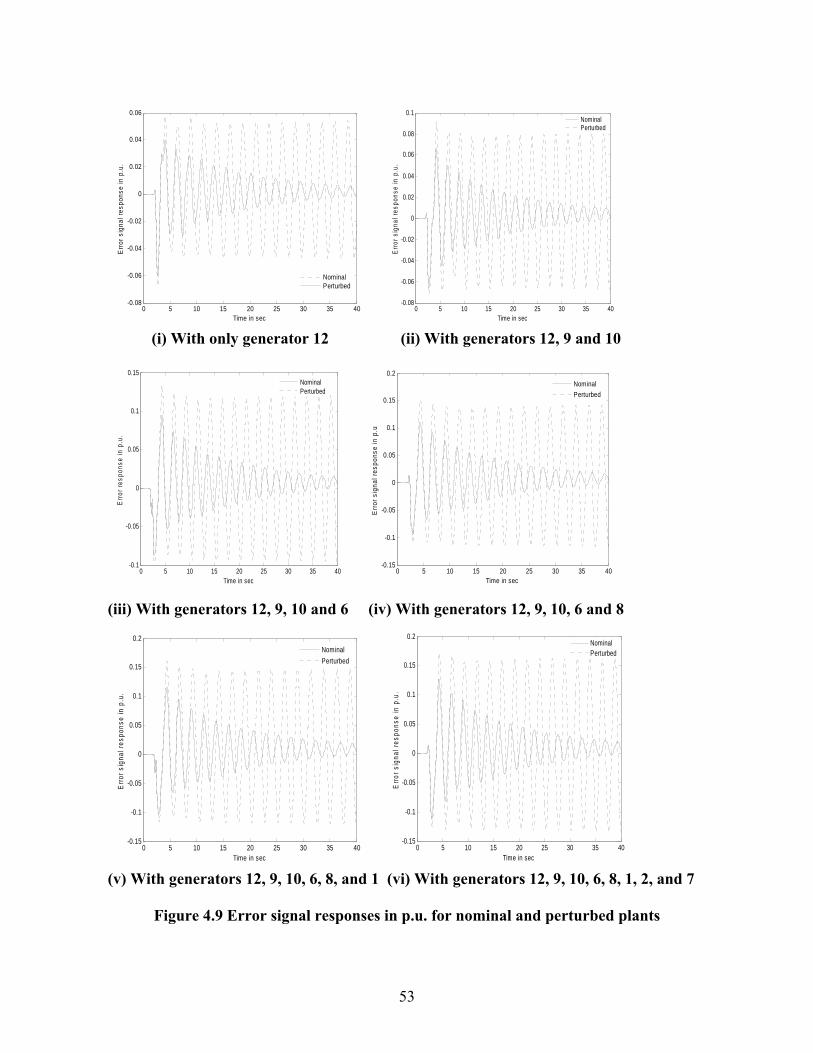
53
0 5 10 15 20 25 30 35 40-0.08
-0.06
-0.04
-0.02
0
0.02
0.04
0.06
Time in sec
Erro
r sig
nal r
espo
nse
in p
.u.
NominalPerturbed
0 5 10 15 20 25 30 35 40-0.08
-0.06
-0.04
-0.02
0
0.02
0.04
0.06
0.08
0.1
Time in sec
Erro
r sig
nal r
espo
nse
in p
.u.
NominalPerturbed
(i) With only generator 12 (ii) With generators 12, 9 and 10
0 5 10 15 20 25 30 35 40-0.1
-0.05
0
0.05
0.1
0.15
Time in sec
Erro
r res
pons
e in
p.u
.
NominalPerturbed
0 5 10 15 20 25 30 35 40-0.15
-0.1
-0.05
0
0.05
0.1
0.15
0.2
Time in sec
Erro
r sig
nal r
espo
nse
in p
.uNominalPerturbed
(iii) With generators 12, 9, 10 and 6 (iv) With generators 12, 9, 10, 6 and 8
0 5 10 15 20 25 30 35 40-0.15
-0.1
-0.05
0
0.05
0.1
0.15
0.2
Time in sec
Erro
r sig
nal r
espo
nse
in p
.u.
NominalPerturbed
0 5 10 15 20 25 30 35 40-0.15
-0.1
-0.05
0
0.05
0.1
0.15
0.2
Time in sec
Erro
r sig
nal r
espo
nse
in p
.u.
NominalPerturbed
(v) With generators 12, 9, 10, 6, 8, and 1 (vi) With generators 12, 9, 10, 6, 8, 1, 2, and 7
Figure 4.9 Error signal responses in p.u. for nominal and perturbed plants

54
4.8.2.1.2. WECC System
The following is another example of the application of SIMGUI in selecting the error signal for the WECC system. In this system, multiple critical oscillatory modes are observed. Table 4.3 shows three critical modes and the generators that significantly participate in these modes for the nominal operating condition under consideration.
Table 4.3 Three critical oscillatory modes of WECC system and their participating generators
S. No. Mode frequency in Hz
Participating generators
1 0.29 4, 8, 9, 15, 18, 24 2 0.88 8, 17, 18, 22 3 1.05 17, 18, 22
With multiple critical oscillatory modes, it is essential to check the choice of the error signal over a range of operating conditions because different modes could get excited at different power flow levels in the system. With SIMGUI, by varying the uncertainty size, it is possible to simulate the error signal response over a range of operating conditions. Also in scenarios where the same generators participate in different modes, the effect of those generators could be different on different modes. In such cases, the combination of generators that best represent the damping over an entire range will have to be chosen. In the following case, two different uncertainty sizes have been examined and have been shown to excite different modes into instability. For the first uncertainty, the worst-case operating condition is such that mode 1 with a frequency of 0.29 Hz becomes unstable. For the second uncertainty, both modes 2 and 3 become unstable. The error signal will have to capture the damping performance at different operating conditions around the nominal operating point. Uncertainty is assumed to exist in the controllable part of the active power load at the following load buses of the system: 5, 62, 66, 106, 107, 117, 137, 141, 143 and 145. Figure 4.10 (i) and (ii) shows the response of the error signal consisting of the angular speeds of generators 8, 17 and 18 for the two different uncertainties. The disturbance input in both the cases is a step change in the excitation system reference voltage of generator 2. With the
performance weight for the error signal, Wperf =189305.4
78.02
2
++ sss
As can be seen from Figure 4.10 (iii) and (iv), accounting for more generators captures the damping characteristics better for the second perturbation. This procedure of checking the error signal responses for every change in the composition of the error signal is repeated for different uncertainty sizes until the final selection of the generators is arrived at. The error

55
signal finally selected consists of the angular speeds of generators 8, 15, 17, 18, and 22. Additional generator speeds do not improve the response significantly over the range of operating conditions.
Table 4.4 Calculated Participation factors for speed and angle states for the three critical oscillatory modes of WECC system
Mode frequency in Hz Generator State Participation factor in % 8 δ 16.43 18 δ 13.34 9 δ 12.63 15 ω 6.29 8 ω 6.25 9 ω 6.03 4 ω 4.45 18 ω 4.04
0.29
24 ω 4.00 8 δ 26.36
8 ω 21.37 18 δ 17.66 18 ω 11.64 22 δ 10.41 22 ω 7.53 17 δ 6.72
0.88
17 ω 6.49 17 δ 29.24
17 ω 28.12 18 δ 12.21 18 ω 10.81 22 ω 4.47
1.05
22 δ 4.14
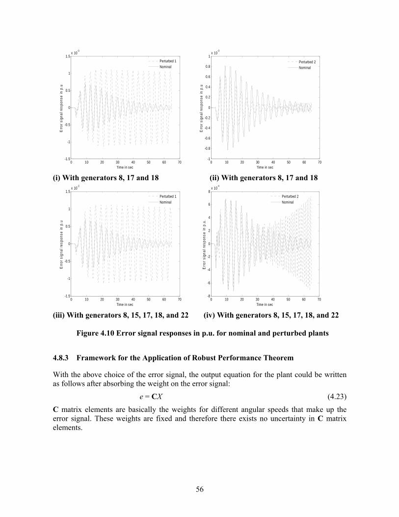
56
0 10 20 30 40 50 60 70-1.5
-1
-0.5
0
0.5
1
1.5x 10
-3
Time in sec
Erro
r sig
nal r
espo
nse
in p
.uPerturbed 1Nominal
0 10 20 30 40 50 60 70-1
-0.8
-0.6
-0.4
-0.2
0
0.2
0.4
0.6
0.8
1x 10
-3
Time in sec
Erro
r sig
nal r
espo
nse
in p
.u
Perturbed 2Nominal
(i) With generators 8, 17 and 18 (ii) With generators 8, 17 and 18
0 10 20 30 40 50 60 70-1.5
-1
-0.5
0
0.5
1
1.5x 10⁻³
Time in sec
Erro
r sig
nal r
espo
nse
in p
.u
Perturbed 1Nominal
0 10 20 30 40 50 60 70-8
-6
-4
-2
0
2
4
6
8x 10⁻⁴
Time in sec
Erro
r sig
nal r
espo
nse
in p
.u.
Perturbed 2Nominal
(iii) With generators 8, 15, 17, 18, and 22 (iv) With generators 8, 15, 17, 18, and 22
Figure 4.10 Error signal responses in p.u. for nominal and perturbed plants
4.8.3 Framework for the Application of Robust Performance Theorem
With the above choice of the error signal, the output equation for the plant could be written as follows after absorbing the weight on the error signal:
e = CX (4.23)
C matrix elements are basically the weights for different angular speeds that make up the error signal. These weights are fixed and therefore there exists no uncertainty in C matrix elements.
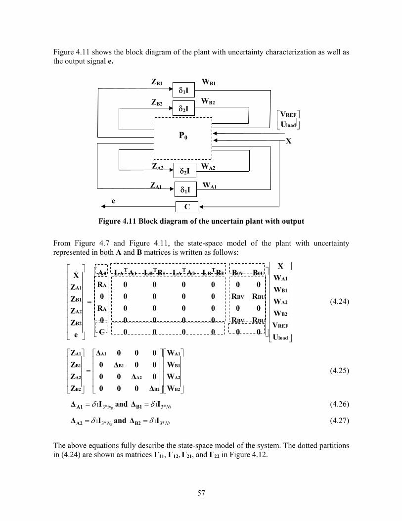
57
Figure 4.11 shows the block diagram of the plant with uncertainty characterization as well as the output signal e.
Figure 4.11 Block diagram of the uncertain plant with output
From Figure 4.7 and Figure 4.11, the state-space model of the plant with uncertainty represented in both A and B matrices is written as follows:
⎥⎥⎥⎥⎥⎥⎥⎥⎥
⎦
⎤
⎢⎢⎢⎢⎢⎢⎢⎢⎢
⎣
⎡
⎥⎥⎥⎥⎥⎥⎥⎥
⎦
⎤
⎢⎢⎢⎢⎢⎢⎢⎢
⎣
⎡
=
⎥⎥⎥⎥⎥⎥⎥⎥
⎦
⎤
⎢⎢⎢⎢⎢⎢⎢⎢
⎣
⎡
load
REF
B2
A2
B1
A1
BUBV
A
BUBV
A
0U0V2T
B2T
A1T
B1T
A0
B2
A2
B1
A1
UVWWWW
X
000000CRR00000
000000RRR00000
000000RBBBLALBLALA
eZZZZX&
(4.24)
⎥⎥⎥⎥
⎦
⎤
⎢⎢⎢⎢
⎣
⎡
⎥⎥⎥⎥
⎦
⎤
⎢⎢⎢⎢
⎣
⎡
=
⎥⎥⎥⎥
⎦
⎤
⎢⎢⎢⎢
⎣
⎡
B2
A2
B1
A1
B2
A2
B1
A1
B2
A2
B1
A1
WWWW
Δ0000Δ0000Δ0000Δ
ZZZZ
(4.25)
gN*31IΔA1 δ= and lN*31IΔB1 δ= (4.26)
gN*31IΔA2 δ= and lN*31IΔB2 δ= (4.27)
The above equations fully describe the state-space model of the system. The dotted partitions in (4.24) are shown as matrices Г11, Г12, Г21, and Г22 in Figure 4.12.
P0
δ1I
δ2I
ZB1
ZB2
WB1
WB2
δ2I
δ1I
ZA2 WA2
WA1 ZA1
⎥⎦⎤
⎢⎣⎡
load
REF
UV
X
C e

58
Figure 4.12 State-space model of the system for robust performance analysis
This state-space model of the uncertain linear model is then expressed in the N-∆ form shown in Figure 4.6 in order to be able to perform robust performance analysis using the SSV theory. This is shown in Figure 4.12 and Figure 4.13. ∆P is a fictitious full-block complex uncertainty of size 1xNg representing the H∞ performance specification and it enables the application of Theorem 4.2, robust performance theorem. The parametric uncertainty, ∆, is a structured uncertainty with real repeated blocks, ∆A1, ∆B1, ∆A2, ∆B2 given by (4.26) and (4.27). In Figure 4.13, the parametric uncertainty is augmented with full block complex uncertainty to result in N-∆ framework. The augmented uncertainty block is again structured:
⎥⎦
⎤⎢⎣
⎡=
⎥⎥⎥⎥⎥⎥
⎦
⎤
⎢⎢⎢⎢⎢⎢
⎣
⎡
=P
P
B2
A2
B1
A1
Δ00Δ
:
Δ00000Δ00000Δ00000Δ00000Δ
Δ (4.28)
The disturbance input in this framework is the vector of exciter reference voltage changes.
s1
⎥⎦
⎤⎢⎣
⎡B
A
ZZ
X&
∆VREF ∆Uload Wperf ⎥
⎥⎥
⎦
⎤
⎢⎢⎢
⎣
⎡
ΓΓΓΓΓΓΓΓΓ
333231
232221
131211
⎥⎥⎥⎥
⎦
⎤
⎢⎢⎢⎢
⎣
⎡
B2
A2
B1
A1
Δ0000Δ0000Δ0000Δ
∆P
X
⎥⎦
⎤⎢⎣
⎡B
A
WW
e
N
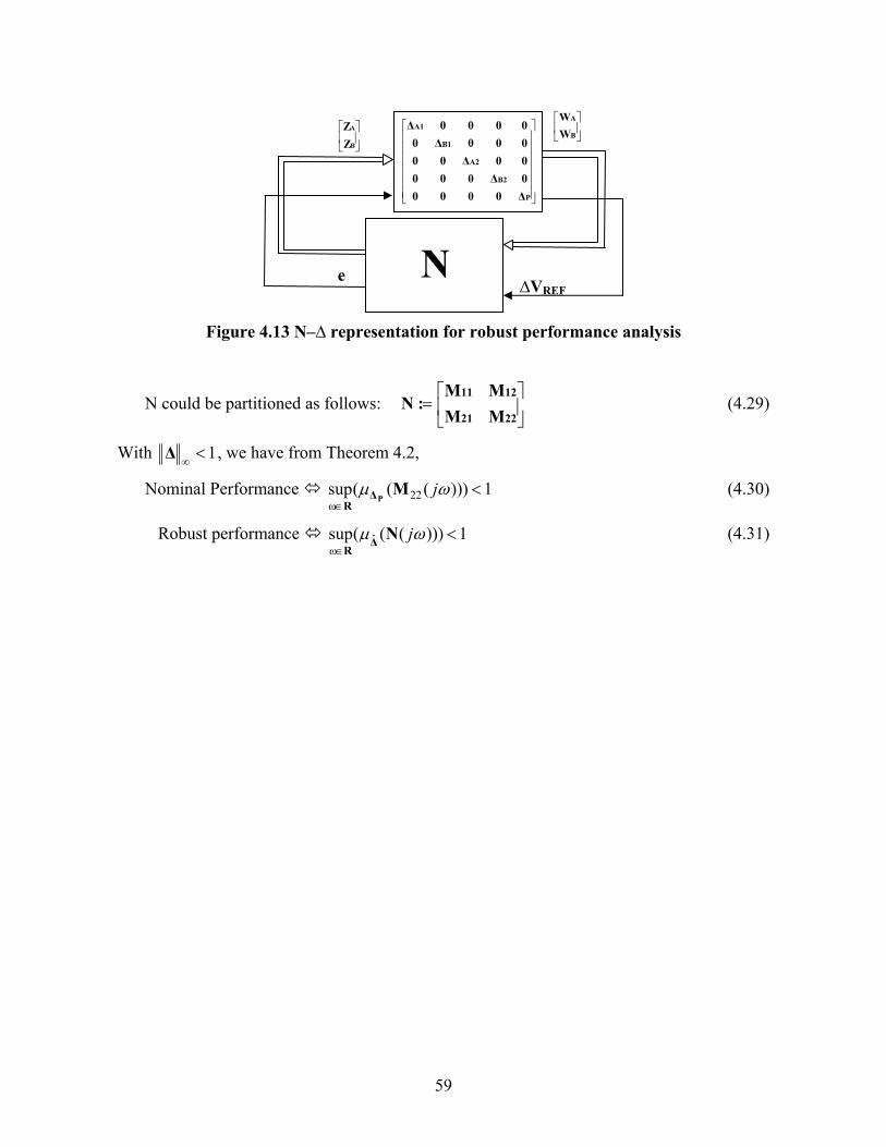
59
Figure 4.13 N–∆ representation for robust performance analysis
N could be partitioned as follows: ⎥⎦
⎤⎢⎣
⎡=
2221
1211
MMMM
:N (4.29)
With 1<∞
Δ , we have from Theorem 4.2,
Nominal Performance 1)))(((sup 22ω
<∈
ωμ jMPΔ
R (4.30)
Robust performance 1)))(((sup ˆω
<∈
ωμ jNΔR
(4.31)
⎥⎦
⎤⎢⎣
⎡B
A
ZZ
N
⎥⎥⎥⎥⎥⎥
⎦
⎤
⎢⎢⎢⎢⎢⎢
⎣
⎡
P
B2
A2
B1
A1
Δ00000Δ00000Δ00000Δ00000Δ
⎥⎦
⎤⎢⎣
⎡B
A
WW
e ∆VREF

60
5. Skewed – μ Based Robust Performance Analysis for Load Modulation
This section discusses in detail two different approaches towards analysis of load modulation for satisfying desired damping performance for the system. The overall objective is the determination of the optimal amount of preventive load modulation for maintaining a desired damping performance for the system. Both these approaches are based on robust performance analysis using the framework developed in the previous section. In the context of SSV theory, the structured singular value bounds calculated in both the approaches, which are used as performance measures, are skewed – μ bounds. This section begins with an overview of modal analysis through the application of eigenvalue sensitivity, applied in the robust performance analysis. Each of the two approaches is then discussed in detail. The algorithms used within the two approaches are also presented. Results are presented on both the Nordic as well as the WECC test systems. The correctness of the formulation of the framework for robust performance analysis as well as the choice of performance characterization and the impact of performance on the amount of active power load modulation are discussed using the results.
5.1 Modal Analysis
Eigenvalue sensitivity for active power loads is applied in the selection of the optimal locations for load modulation in the system. Depending on the modal participation factors of state variables as well as the impact of active power loads at different locations on the powerflow pattern in the interconnected system, different loads have varying sensitivities for eigenvalues. The power system linear model developed in Section 3 can be used to study the sensitivity of each candidate load bus on different oscillatory modes. The load buses that exhibit the highest sensitivities for the real part of the critical oscillatory modes under consideration would be the best location to improve overall system dynamic performance to the desired level with minimum load modulation. In the sequel, in both approaches towards analysis of the amount of load modulation, load buses that exhibit highest sensitivities for critical oscillatory modes are selected. It has been observed that, depending on the operating conditions as well as the system configuration, the sensitivities of loads could either be positive or negative. That is, under certain conditions, increase in the load at a certain bus could improve the dynamic performance with respect to oscillatory modes. This is clearly evident in the results for eigenvalue sensitivities obtained for both the Nordic as well as the WECC test systems.
5.1.1 Eigenvalue Sensitivities
Consider the dynamical system governed by the state equation of the form
BUAXX +=& (5.1)
Let A be an nn× state-matrix with distinct eigenvalues λi (i = 1, 2,.., n). Let ui be the linearly independent eigenvectors of A which satisfy
ii uAu iλ= (5.2)

61
and vj (j = 1, 2,..,n) are the corresponding eigenvectors of A′ which satisfy
jjj λ vvA =′ (5.3)
The ui and vj satisfy the following:
ijijj δ=′=′ uvvui i,j = 1, 2,..,n (5.4)
If
[ ]kla=A
and the generic element akl is perturbed due to changes in system parameters, then the eigenvalues and eigenvectors of A will change. Indeed, partial differentiation of (5.2) with respect to akl indicates that
kl
iii
kl
i
kl
ii
kl aaaa ∂∂
+∂∂
=∂∂
+∂∂ uuuAuA λλ (5.5)
Pre-multiplication of (5.5) by iv′ then gives
kl
iiii
kl
ii
kl
iiii
kli aaaa ∂
∂′+∂∂′=
∂∂′+
∂∂′ uvuvuvuAv λλλ (5.6)
which reduces to the set of scalar equations l
ik
ikl
i uva
=∂∂λ (5.7)
i, k, l = 1,2, …,n
in view of the (5.4) and the fact that
[ ] jlikijkla
δδα ==∂∂A (5.8)
The ∂λi/∂akl are the desired eigenvalue sensitivity coefficients which relate changes in λi to changes in the akl. These coefficients may be viewed as the elements of a set of n eigenvalue sensitivity matrices
iikl
i
auvSi ′=⎥
⎦
⎤⎢⎣
⎡∂∂
=λ i, k, l = 1,2,..,n (5.9)
In order to calculate eigenvalue sensitivity for active power loads, the sensitivity of A matrix elements with respect to active power loads needs to be determined first. This is already available as part of the robust performance analysis framework developed earlier. Precisely, the variation of each A matrix element as a result of the change in active power load is expressed as in (4.18).
][ iloadiload
kl
kl
i aPa
auvSi ′=⎥
⎦
⎤⎢⎣
⎡∂∂
∂∂
=λ i, k, l = 1,2,..,n ` (5.10)
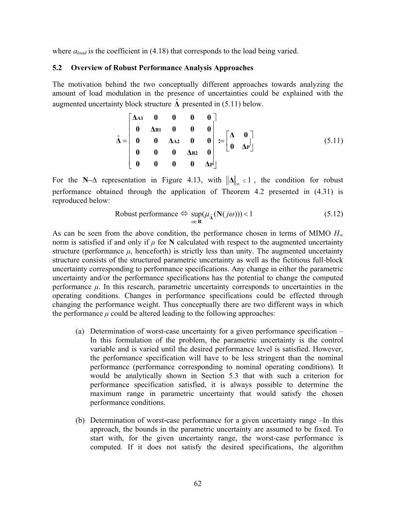
62
where aload is the coefficient in (4.18) that corresponds to the load being varied.
5.2 Overview of Robust Performance Analysis Approaches
The motivation behind the two conceptually different approaches towards analyzing the amount of load modulation in the presence of uncertainties could be explained with the augmented uncertainty block structure Δ presented in (5.11) below.
⎥⎦
⎤⎢⎣
⎡=
⎥⎥⎥⎥⎥⎥
⎦
⎤
⎢⎢⎢⎢⎢⎢
⎣
⎡
=P
P
B2
A2
B1
A1
Δ00Δ
:
Δ00000Δ00000Δ00000Δ00000Δ
Δ (5.11)
For the N–∆ representation in Figure 4.13, with 1≤∞
Δ , the condition for robust performance obtained through the application of Theorem 4.2 presented in (4.31) is reproduced below:
Robust performance 1)))(((sup ˆω
<∈
ωμ jNΔR
(5.12)
As can be seen from the above condition, the performance chosen in terms of MIMO H∞ norm is satisfied if and only if μ for N calculated with respect to the augmented uncertainty structure (performance μ, henceforth) is strictly less than unity. The augmented uncertainty structure consists of the structured parametric uncertainty as well as the fictitious full-block uncertainty corresponding to performance specifications. Any change in either the parametric uncertainty and/or the performance specifications has the potential to change the computed performance μ. In this research, parametric uncertainty corresponds to uncertainties in the operating conditions. Changes in performance specifications could be effected through changing the performance weight. Thus conceptually there are two different ways in which the performance μ could be altered leading to the following approaches:
(a) Determination of worst-case uncertainty for a given performance specification – In this formulation of the problem, the parametric uncertainty is the control variable and is varied until the desired performance level is satisfied. However, the performance specification will have to be less stringent than the nominal performance (performance corresponding to nominal operating conditions). It would be analytically shown in Section 5.3 that with such a criterion for performance specification satisfied, it is always possible to determine the maximum range in parametric uncertainty that would satisfy the chosen performance conditions.
(b) Determination of worst-case performance for a given uncertainty range –In this
approach, the bounds in the parametric uncertainty are assumed to be fixed. To start with, for the given uncertainty range, the worst-case performance is computed. If it does not satisfy the desired specifications, the algorithm

63
modulates the load levels at selected load buses in the system. The load modulation is iterative and is performed until the load level in the system is such that the chosen performance specifications are satisfied for the uncertainty range under consideration. The selection of load buses for control implementation is based on the eigenvalue sensitivity of active power loads. Essentially, in this approach, the nominal load levels at certain load buses are the control variables and they are varied until the worst-case performance for the fixed uncertainty range is satisfied.
Thus, both the approaches determine the amount of load modulation to be performed to satisfy the chosen damping performance criterion, however in complimentary ways. In the first approach, the parametric uncertainty is also the control variable. This necessitates the assumption of uncertainty in the active power loads. In the second approach, nominal load levels are the control variables resulting in a relatively general uncertainty representation. In both the approaches, eigenvalue sensitivity is applied in the selection of loads for control implementation. The performance μ computed is skewed – μ in both the cases. In the first approach, only the parametric uncertainty part is controlled. In contrast, in the second approach, the parametric uncertainty is kept fixed and the analysis determines the worst-case performance through varying the size of the full-block complex uncertainty. This is indirectly accomplished through the control of performance weight. As a consequence of the computed performance μ being skewed, the determination of the worst-case uncertainty in the first approach and the worst-case performance in the second approach are both iterative. This is explained in more detail in the following sections.
5.3 Approach I – Determination of Worst-case Uncertainty for Fixed Performance
The following are three fundamental aspects with respect to Approach I:
i) Uncertainty is assumed to exist in the controllable part of the load. ii) Uncertainty in controllable load at selected load buses is varied until the desired
performance specifications are met. iii) The performance specifications have to be chosen such that they are always
satisfied at nominal load levels. Based on eigenvalue sensitivities, certain load buses are selected in the system for control implementation. The active power load at each of these load buses is made of controllable and uncontrollable parts. The reactive power load is assumed to be entirely uncontrollable. Uncertainty is assumed to exist in the controllable part of the active power load. The uncontrollable part of the real power load is assumed to be known with certainty. Also it is assumed that no uncertainty exists in the entire reactive power load. Load model for active power load presented in (3.38) is reproduced below:

64
pi
ii
pi
iiii
VVP
VVPUP i
UKi
KloadL
βα
⎟⎠⎞
⎜⎝⎛
⎟⎠⎞
⎜⎝⎛= +
0000 ; i = Ng+1, 2, 3, …., Ng+Nld (5.13)
where, PK0i is the controllable part of the load, and PUK0i is the uncontrollable part of the load at bus i. PK0i is assumed to be in the range [ ]max
0min
0 ii KK PP − resulting in PLi to be in the range [ ]maxmin
ii LL PP − . With NC load buses selected for control implementation, there are as many independent parameters, and hence as many underlying uncertainties, CNδδδ ,....,, 21 ; 1≤iδ , i=1,..NC. However, in order to reduce the dimensionality of the problem, correlation among some of the controllable loads could be assumed which would reduce the number of underlying uncertainties. Following the procedure explained in Section 4.8.1, entire A and B matrices could be expressed in the LFT form. This is done by essentially forming a reasonably dense grid of operating points in terms of the controllable loads, executing power flows for different points on the grid, forming the A and B matrices for these points, and expressing the varying elements of A and B matrices in terms of the underlying uncertainties through a least squares curve fit. Without loss of generality, two independent underlying uncertainties have been assumed in the augmented uncertainty structure shown in (5.11) and considered below. Starting with an uncertain range of controllable loads, when the uncertainty in load levels is scaled up (or down), the real repeated uncertainty blocks ∆A1, ∆B1, ∆A2 and ∆B2 are correspondingly scaled up (or down). However, the performance weights are kept fixed. The performance μ is computed with respect to the augmented uncertainty. If it is greater (or less) than unity, then scaling down (or up) ∆A1, ∆B1, ∆A2 and ∆B2 as well as the performance weight would result in the new value for the performance μ exactly equal to unity. However, since in the present approach, the performance weights are not changed, the value for the performance μ after scaling the parametric uncertainty blocks would not be unity. In the sequel, it is analytically shown that with the performance specification chosen less stringent than the nominal performance (that is performance obtained with no uncertainty, i.e. with ∆A1 ≡ 0, ∆B1 ≡ 0, ∆A2 ≡ 0 and ∆B2 ≡ 0), starting with an arbitrary range for parametric uncertainty it is possible to arrive at a worst-case range that exactly satisfies the chosen performance specifications. This process requires iterating on the size of the parametric uncertainty. The definition for μ is related to the size of the entire uncertainty block, but the calculated performance μ is skewed as only a part of the overall uncertainty structure is being controlled. As was stated in Section 4.7, μs is always further from 1 than μ is. When the real repeated uncertainty blocks are scaled down (or up), the full-block uncertainty could be, in a general sense, of a size such that μ for the augmented uncertainty is not correspondingly scaled down (or up). However, with a suitably chosen performance specification, it can be shown that the desired performance μ can be obtained by controlling only the parametric uncertainty. A robust performance specification that is less stringent than
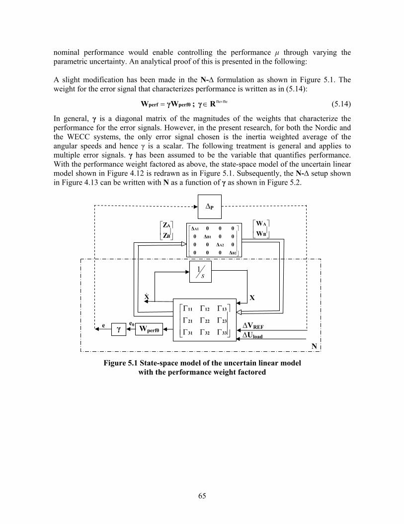
65
nominal performance would enable controlling the performance μ through varying the parametric uncertainty. An analytical proof of this is presented in the following:
A slight modification has been made in the N-∆ formulation as shown in Figure 5.1. The weight for the error signal that characterizes performance is written as in (5.14):
perf0perf γWW = ; ee nn ×∈Rγ (5.14)
In general, γ is a diagonal matrix of the magnitudes of the weights that characterize the performance for the error signals. However, in the present research, for both the Nordic and the WECC systems, the only error signal chosen is the inertia weighted average of the angular speeds and hence γ is a scalar. The following treatment is general and applies to multiple error signals. γ has been assumed to be the variable that quantifies performance. With the performance weight factored as above, the state-space model of the uncertain linear model shown in Figure 4.12 is redrawn as in Figure 5.1. Subsequently, the N-∆ setup shown in Figure 4.13 can be written with N as a function of γ as shown in Figure 5.2.
Figure 5.1 State-space model of the uncertain linear model
with the performance weight factored
s1
⎥⎦
⎤⎢⎣
⎡B
A
ZZ
X&
∆VREF ∆Uload
Wperf0 ⎥⎥⎥
⎦
⎤
⎢⎢⎢
⎣
⎡
ΓΓΓΓΓΓΓΓΓ
333231
232221
131211
⎥⎥⎥⎥
⎦
⎤
⎢⎢⎢⎢
⎣
⎡
B2
A2
B1
A1
Δ0000Δ0000Δ0000Δ
∆P
X
⎥⎦
⎤⎢⎣
⎡B
A
WW
e
N
γ e0

66
Figure 5.2 N–∆ representation for robust performance analysis with N as a function of γ The robust performance condition and the nominal performance conditions in (4.31) and (4.30) are rewritten as in (5.15) and (5.16): With 1≤
∞Δ ,
Robust performance 1)))(((sup ˆω
<∈
γNΔRμ (5.15)
Nominal performance 1)))(((supω
<∈
γM22ΔR
Pμ (5.16)
with N(γ) is partitioned as
( ) ( ) ( )( ) ( )⎥⎦
⎤⎢⎣
⎡=
γMγMγMγM
:γN2221
1211 (5.17)
Let ee nn ×∈Rγnom be such that
1)))(((supω
=∈
nom22ΔR
γMP
μ (5.18)
From the definition of μ for full-block complex uncertainty in (4.5), it follows that such that ed nn ×∈′∃ CΔP
( )⎭⎬⎫
=′=′
0))(det(and σ
Pnom
P
ΔγM-I1Δ
22
(5.19)
that is, the nominal system exactly satisfies the performance weights with magnitudes nomγ and thus nomγ defines the nominal performance of the system.
Suppose ee nn ×∈Rγrp and nomrp γγ ≠ . Then,
( ) 10))(det(:σinf ≠=PrpP ΔγM-IΔ 22 (5.20)
⎥⎦
⎤⎢⎣
⎡B
A
ZZ
)(γN
⎥⎥⎥⎥⎥⎥
⎦
⎤
⎢⎢⎢⎢⎢⎢
⎣
⎡
P
B2
A2
B1
A1
Δ00000Δ00000Δ00000Δ00000Δ ⎥
⎦
⎤⎢⎣
⎡B
A
WW
e0 ∆VREF

67
Suppose rpγ be such that
( ) 10))(det(:σinf <=PrpP ΔγM-IΔ 22 (5.21)
Then nominal performance is not satisfied with rpγ as the magnitude of weights. Hence
rpγ has to be such that
( ) 10))(det(:σinf >=PrpP ΔγM-IΔ 22 (5.22)
Claim With rpγ chosen as in (5.22), and with PΔ′ as in (5.19),
sΔΔ∈∃ in (4.12) with 0Δ ≠ in ⎥⎦
⎤⎢⎣
⎡′
=′PΔ0
0ΔΔ
such that 0)ˆ)(det( =′ΔγN-I rp .
Hence 0)ˆ)((det:)ˆ(σinf
1))((ˆ=
=ΔγN-IΔ
γNrp
rpΔμ
Proof
)ˆ(σ0)ˆ)(det(:)ˆ(σinf ΔΔγN-IΔ rp ′== (5.23)
implies that
0)ˆ)(det( =′ΔγN-I rp (5.24)
( ) ( )( ) ( ) 0det =⎟
⎟⎠
⎞⎜⎜⎝
⎛⎥⎦
⎤⎢⎣
⎡′⎥
⎦
⎤⎢⎣
⎡⎥⎦
⎤⎢⎣
⎡
Prp22rp21
rp12rp11
Δ00Δ
γMγMγMγM
-I00I
(5.25)
( ) ( )( ) ( ) 0det =⎟
⎟⎠
⎞⎜⎜⎝
⎛⎥⎦
⎤⎢⎣
⎡′−−
′−−
Prp22rp21
Prp12rp11
ΔγMIΔγMΔγMΔγMI
(5.26)
Applying Schur’s formula for the determinant of a partitioned matrix,
( ) ( )( ) ( ) ⎟
⎟⎠
⎞⎜⎜⎝
⎛⎥⎦
⎤⎢⎣
⎡′−−
′−−
Prp22rp21
Prp12rp11
ΔγMIΔγMΔγMΔγMI
det =
( )( )×′− Prp22 ΔγMIdet
( ) ( )( ) ( )( ) ( )( )( ) 0det 1 =−′−′−−− − ΔγMΔγMIΔγMΔγMI rp21Prp22Prp12rp11 (5.27)

68
Since nomrp γγ ≠ and from (5.20)
( )( ) 0det ≠′− Prp22 ΔγMI (5.28)
Hence ( )( ) 1−′− Prp22 ΔγMI exists. Hence
( ) ( )( ) ( )( ) ( )( )( ) 0det 1 =−′−′−−− − ΔγMΔγMIΔγMΔγMI rp21Prp22Prp12rp11 (5.29)
Suppose 0Δ = Then ( ) ( )( ) ( )( ) ( )( )( ) 0detdet 1 ≠=−′−′−−− − (I)ΔγMΔγMIΔγMΔγMI rp21Prp22Prp12rp11
Contradiction
Hence 0Δ ≠ in ⎥⎦
⎤⎢⎣
⎡′
=′PΔ0
0ΔΔ when 0)ˆ)(det( =′ΔγN-I rp
The performance μ of the system with performance as defined by rpγ corresponding to given parametric uncertainty Δ could then be determined as the smallest augmented uncertainty ( Δ ) measured in terms of )ˆ(σ Δ that makes .0)ˆ)(det( =ΔγN-I rp
0)ˆ)((det:)ˆ(σinf1))((ˆ
==
ΔγN-IΔγN
rprpΔμ (5.30)
Thus a performance less stringent than nominal performance could be satisfied in the presence of parametric uncertainty.
In practice, the approach that could be adopted is to examine the system dynamic performance at a variety of off-peak operating conditions, and choose a certain reasonable damping requirement that is less stringent than one of those off-peak operating conditions. The corresponding uncontrollable load level in the system could then be chosen as the nominal load levels. Around this nominal load level, uncertainty could be assumed for the controllable load levels, with the controllable loads modeled with their appropriate load models at selected buses. Robust performance analysis following the present approach would then yield the worst-case uncertainty in the controllable load levels that would satisfy the chosen performance. The performance weights could be subsequently varied to determine the impact on the worst-case uncertainty range as well as the total load levels. Through repeatedly executing robust performance analysis for different nominal as well as uncertain ranges for the controllable load levels (but with fixed performance weight), a performance boundary could be obtained in terms of system load levels at buses selected for control. This boundary would define different combinations of operating load levels that would result in the same dynamic performance for the interconnected system. This has been demonstrated with the Nordic system in this section.

69
5.3.1 Algorithm for Approach I
Following is the algorithm for Approach I – Determination of worst-case uncertainty for fixed performance.
i) Select the load buses for control implementation based on eigenvalue sensitivities from active power loads.
ii) Form a reasonably dense grid of operating points in terms of the controllable load levels at each of the above selected buses. The controllable part of the active power load is assumed to be uncertain in a range at each load bus. It has been verified that consideration of three points (minimum, nominal, and maximum) in the uncertainty range for each active power load is sufficient.
iii) Execute power flows corresponding to different combinations of minimum, nominal and maximum operating points for the different uncertain load levels.
iv) Form the linear model (A and B matrices) for each operating point in the grid v) Calculate linear curve-fitting coefficients for each varying element of the A and B
matrices, to be expressed in terms of the underlying uncertainties. vi) Express the uncertain system in N-Δ framework for robust performance analysis
by characterizing the uncertainty in LFT form and characterizing performance through weighted error signals, as explained in Section 4.8.
vii) Calculate the upper bound of performance μ. Check the following conditions (a) – (c). a. If computed performance μ upper bound >1, scale down the parametric
uncertainty in the controllable load levels by the upper bound of performance μ. Repeat steps (ii) – (vii).
b. If computed performance μ upper bound <1, scale down the parametric uncertainty in the controllable load levels by the upper bound of performance μ. Repeat steps (ii) – (vii).
c. If 1-εμ < computed performance μ upper bound < 1+ εμ, the performance specification is satisfied (within a tolerance εμ for the μ bound) for the uncertainty range at hand.
It has been found that for small changes in the uncertainty ranges in step (vii), i.e. when the performance μ upper bound is not much larger than unity, the linear curve-fitting coefficients need not be updated. This implies that when scaling down or up the uncertainty range in step (vii) above, steps (ii) – (vi) need not be repeated and only step (vi) needs to be executed. This simplification saves considerable execution time in the overall algorithm and has been verified with both Nordic as well as WECC test systems. Figure 5.3 presents flow-chart of the algorithm for approach I.

70
Figure 5.3 Flowchart of the algorithm for approach I – Determination of worst-case uncertainty for given performance
Stop
Calculate performance μ upper bound (μUB)
μUB > 1+εμ
1-εμ< μUB < 1+εμ
Scale down uncertainty range
of controllable loads by a factor
of μUB
Scale up uncertainty range
of controllable loads by a factor
of μUB
Execute Powerflows corresponding to different combinations of minimum,
nominal and maximum load levels in the uncertainty ranges at different selected load buses
Form A and B matrices for the different operating points
considered in the previous step
Calculate linear curve-fitting coefficients for each varying
element of the A and B matrices
Express the system in N-Δ framework through uncertainty representation in LFT form and performance characterization
Calculate Eigenvalue sensitivities for active power loads
Select load buses for control implementation based on Eigenvalue sensitivities
Start
No
Yes
Yes No

71
5.3.2 Approach I – Numerical Simulations and Results
5.3.2.1 Results on Nordic System
In the following section, the results obtained on the Nordic test system are presented. The base case load and generation levels for the subsequent set of results are provided in Appendix B. The various oscillatory modes and the generators that participate in these modes for the base case operating condition are shown in Table 4.1. For this operating condition, the least damped critical oscillatory mode is observed to be mode 7, shown in Table 4.1, with a frequency of approximately 0.4 Hz. Table 5.1 shows the eigenvalue sensitivities for different active power loads for this mode at the base case operating condition.
Table 5.1 Eigenvalue sensitivities of active power loads for critical oscillatory mode (Mode 7) for Nordic system
Load bus Eigenvalue sensitivity N1011 0.0002±j0.0006 N2031 0.0016±j0.002 N1041 0.0025±j0.0031 N1044 0.0021±j0.0027 N1045 0.0022±j0.0029 N41 0.0021±j0.0027 N42 0.0021±j0.0026 N43 0.0021±j0.0027 N46 0.0022±j0.0027 N47 0.0022±j0.0027 N51 0.0022±j0.0029 N61 0.0022±j0.0029 N62 0.0020±j0.0028 N63 0.0019±j0.0029
As can be seen from Table 5.1, different load buses in the Nordic system, except N1011, have more or less similar sensitivities for the critical oscillatory mode under consideration. Figure 5.4 shows the generators (circled) that participate significantly in the
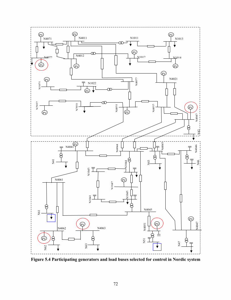
72
Figure 5.4 Participating generators and load buses selected for control in Nordic system
PV
PV PV PV N
2032
PV
PV
PV
PV
PV PV
PV
PV
PVPV
PV
PV PV
N4071 N4011
N4072 N4012
N1011
N1012
N1013
N1014
N10
21 N1022 N40
22 N4021 N
2031
N40
31
N40
32
N4041
N42
PV
N40
43
N40
46
N43
N46
N
4042
N40
44
N10
41N
1043
N10
44
N10
42
N10
45
N41
N4061
N61
N4062
N62
N40
51
N51
N40
47
N47
N4045
PV
N63
N4063

73
above critical oscillatory mode. As can be seen, most of the loads in the system are in the lower region and the effect of increase of these loads is to increase the power flow out of the upper region rich in generation to the lower region rich in load. This explains the uniform positive sensitivities of different loads except N1011. Based on the eigenvalue sensitivities, as well as the amount of active power load available, buses N51 and N61 at 130 KV level have been selected for control implementation. The Nordic system at the transmission level is then augmented with five feeders of the configuration provided in Appendix A at each of the buses, N51 and N61. This is illustrated in Figure 5.5 below. Thus, in all, two load buses at 130 KV level (N51 and N61), 10 load buses at 46.5 KV level (S51_1 – S51_5, S61_1 – S61_5) and 10 more load buses at 13 KV level (D51_1 – D51_5, D61_1 – D61_5) are available for control implementation. In the following results, two underlying uncertainty sources have been assumed. The controllable loads at all voltage levels have been modeled as constant power loads. The uncontrollable loads are modeled as constant impedance loads.
Figure 5.5 Nordic system augmented with sub-transmission/distribution feeders at load buses N51 and N61 at 130 KV level
In the following, different set of results have been shown on the Nordic system augmented with sub-transmission/distribution feeders that clearly demonstrate the following:
i) correctness of the robust performance analysis framework ii) correctness of the choice of error signal for performance characterization iii) correctness of the choice of performance weight.
A performance weight is chosen through trial and error based on different nominal operating conditions. The increase in the performance measure has been found to have the effect of increasing the damping ratios for the critical oscillatory modes. Thus in the choice as well as the validation of different performance weights, the damping ratios corresponding to the
S51_1 S51_2 S51_3 S51_4 S51_5
D51_1 D51_2 D51_3 D51_4 D51_5
46.5 KV
13 KV
130 KV N51
S61_1 S61_2 S61_3 S61_4 S61_5
D61_1 D61_2 D61_3 D61_4 D61_5
46.5 KV
13 KV
130 KV N61

74
critical oscillatory modes have been applied as indices to assess the impact of performance weights on the small-signal stability performance. This has been illustrated in the results shown below. For the base case operating condition, as explained in Section 4.8.2.1.1, through the application of SIMGUI, the weighted average of the angular speeds of generators 6, 8, 9, 10 and 12 has been chosen as the error signal. Also, by comparing different weighting functions for the error signal at several different operating conditions, the following performance weight has been chosen:
2010145.0Wperf
++
=ss (5.31)
It has been observed that the above weighting function for the performance when satisfied, results in 2% damping for the critical oscillatory mode around 0.4 Hz. Several test results have been presented on the Nordic system. In each case, the uncertainty sizes of the controllable load levels as well as the nominal load and/or generation levels have been drastically varied. It has been demonstrated that when the chosen performance is satisfied through the control of uncertainty in load levels, that is, when the performance μ upper bound is unity (within a tolerance of εμ), the damping ratio corresponding to the critical oscillatory mode is always the desired 2%, thereby showing the correctness of the overall setup, correctness of the choice of error signal and performance weight over a range of nominal and uncertain operating conditions. This also demonstrates the robustness of the approach towards determination of the amount of load modulation. Given different nominal load levels and an uncertainty range for certain loads, the approach, by iteratively varying the uncertainty in the controllable loads, determines the load levels that result in the chosen performance specification being exactly satisfied. The effect of a change in performance weight, and the determination of a desired performance boundary in terms of certain selected loads in the system have also been illustrated in the following results. The tolerance allowed on the performance μ upper bound, εμ, is assumed to be 0.02 in the following results.
5.3.2.1.1. Case – 1
The nominal uncontrollable load levels and the uncertain ranges of the controllable load levels at the load buses selected for control are shown in Table 5.2 for this case. The least damped eigenvalue corresponding to the above nominal load levels is – 0.1282 ± j3.0529. The least damped eigenvalue corresponding to the worst-case uncertainty is 0.0905 ± j2.3706. Thus the system, although nominally stable, is clearly robustly unstable.

75
Table 5.2 Nominal and uncertain load levels for case – 1 (Nordic system)
Bus/Buses Uncontrollable load in MW
Uncertain range of controllable load in MW
Uncertain range of total load in MW
N51 60 [-40 – 40] [20 – 100] N61 120 [-90 – 90] [30 – 210]
S51_1 – S51_5 40 [-15 – 15] [25 – 55] D51_1 – D51_5 20 [-5 – 5] [15 – 25] S61_1 – S61_5 40 [-15 – 15] [25 – 55] D61_1 – D61_5 20 [-5 – 5] [15 – 25]
Figure 5.6 shows the performance μ upper and lower bounds over a frequency range from 0.16 Hz (1 rad/s) to 1.6 Hz (10 rad/s) that covers most of the oscillatory modes. As can be seen, the performance μ, although significant at several frequencies in this range, peaks above unity around 0.4 Hz (2.5 rad/s) corresponding to the critical oscillatory mode being considered.
1 2 3 4 5 6 7 8 9 100
0.2
0.4
0.6
0.8
1
1.2
1.4
Frequency in rad/s
Per
form
ance
MU
bou
nds
Figure 5.6 Performance μ bounds for Case – 1 (Nordic system)
Starting with the above uncertainty ranges, algorithm for approach I is applied until the performance μ is unity. Figure 5.7 shows the iteration by iteration convergence of performance μ upper bound to unity for the above case, as the parametric uncertainty in
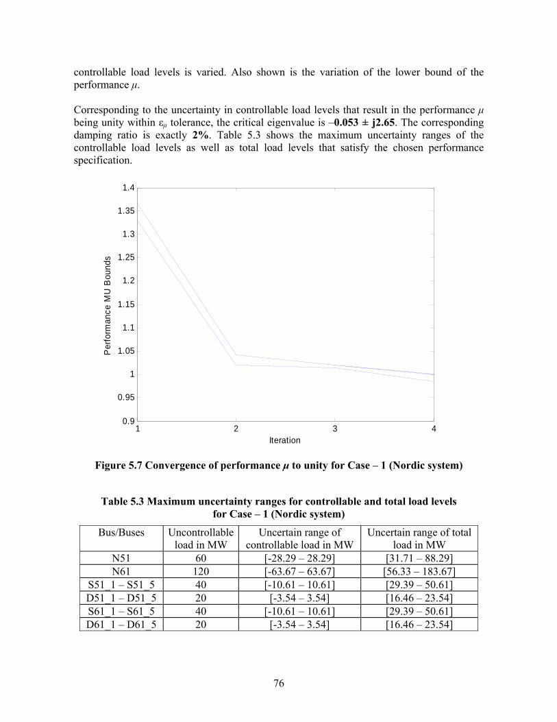
76
controllable load levels is varied. Also shown is the variation of the lower bound of the performance μ. Corresponding to the uncertainty in controllable load levels that result in the performance μ being unity within εμ tolerance, the critical eigenvalue is –0.053 ± j2.65. The corresponding damping ratio is exactly 2%. Table 5.3 shows the maximum uncertainty ranges of the controllable load levels as well as total load levels that satisfy the chosen performance specification.
1 2 3 40.9
0.95
1
1.05
1.1
1.15
1.2
1.25
1.3
1.35
1.4
Iteration
Per
form
ance
MU
Bou
nds
Figure 5.7 Convergence of performance μ to unity for Case – 1 (Nordic system)
Table 5.3 Maximum uncertainty ranges for controllable and total load levels for Case – 1 (Nordic system)
Bus/Buses Uncontrollable load in MW
Uncertain range of controllable load in MW
Uncertain range of total load in MW
N51 60 [-28.29 – 28.29] [31.71 – 88.29] N61 120 [-63.67 – 63.67] [56.33 – 183.67]
S51_1 – S51_5 40 [-10.61 – 10.61] [29.39 – 50.61] D51_1 – D51_5 20 [-3.54 – 3.54] [16.46 – 23.54] S61_1 – S61_5 40 [-10.61 – 10.61] [29.39 – 50.61] D61_1 – D61_5 20 [-3.54 – 3.54] [16.46 – 23.54]

77
Matlab’s MU tools command wcperf offers a way to determine the size of the structured uncertainty that causes the worst-case performance degradation. This has been explained as follows: For perturbations of a particular structure Δs, and of size ≤ α, the worst-case performance possible (as measured in
∞norm) and the perturbation that causes the largest
degradation of performance can be determined. Precisely, given α > 0, the worst-case performance associated with structured performance of size α is defined as
∞
∈
≤= Δ),(max:),Δ,(
sΔΔ
)]Δ([maxMFMW U
j αωσω
α (5.32)
The perturbation matrix which achieves the maximum is denoted as αwc,Δ .The command wcperf assumes that the performance transfer function is an upper loop LFT. The plot of W(M,α) versus α is called the worst-case performance tradeoff curve and it shows the tradeoff between size of uncertainty and the worst-case performance. Since the exact value of μ cannot be calculated and it can only be bounded, the command wcperf returns the upper and lower bounds of the worst-case uncertainty. The worst-case perturbation has a norm equal to α. The command, wcperf, offers an alternative way to compute the worst-case uncertainty for a given performance measure and is used here as the basis for comparing the results obtained using the algorithm proposed.
0 0.5 1 1.5 2 2.5 3 3.50
0.2
0.4
0.6
0.8
1
1.2
1.4
1.6
1.8
Perturbation size
Wor
st-c
ase
Per
form
ance
Nor
m B
ound
s
Figure 5.8 Worst-case performance trade-off curve for Case – 1 (Nordic system)
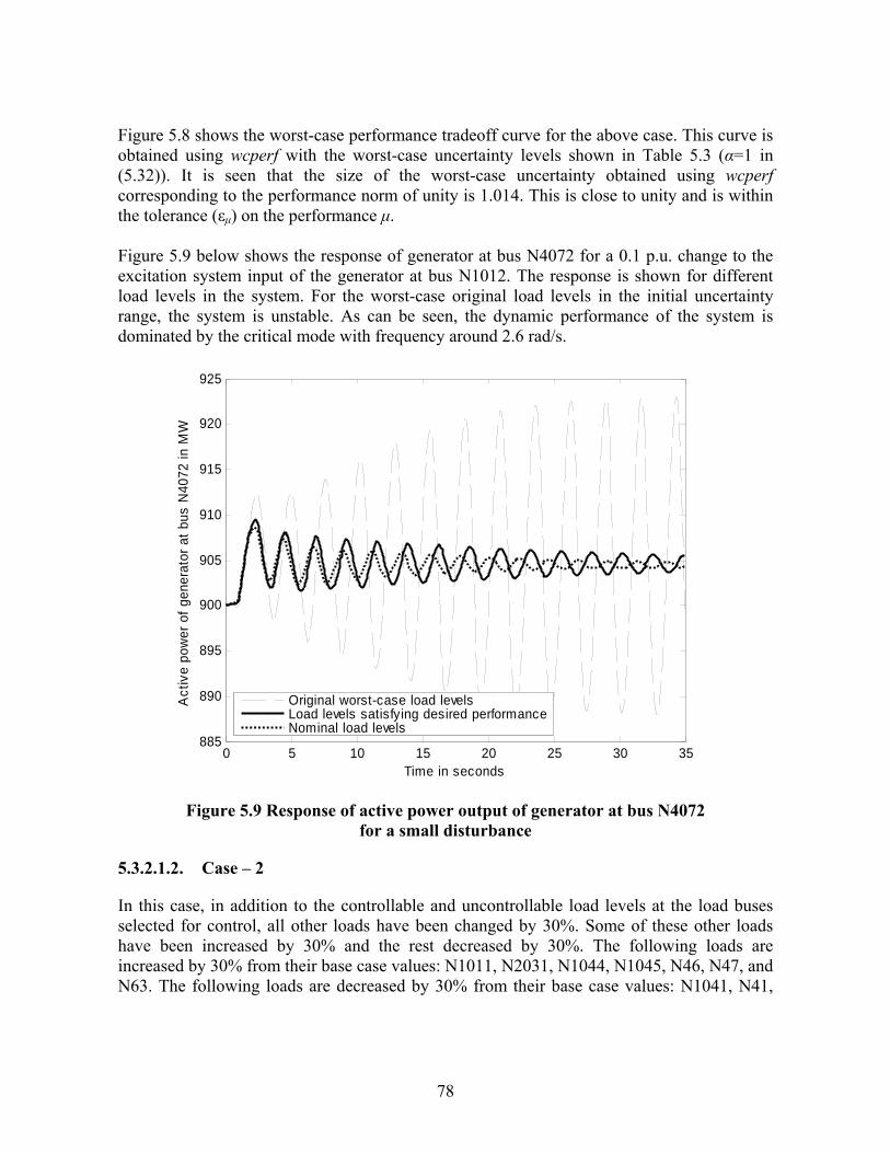
78
Figure 5.8 shows the worst-case performance tradeoff curve for the above case. This curve is obtained using wcperf with the worst-case uncertainty levels shown in Table 5.3 (α=1 in (5.32)). It is seen that the size of the worst-case uncertainty obtained using wcperf corresponding to the performance norm of unity is 1.014. This is close to unity and is within the tolerance (εμ) on the performance μ. Figure 5.9 below shows the response of generator at bus N4072 for a 0.1 p.u. change to the excitation system input of the generator at bus N1012. The response is shown for different load levels in the system. For the worst-case original load levels in the initial uncertainty range, the system is unstable. As can be seen, the dynamic performance of the system is dominated by the critical mode with frequency around 2.6 rad/s.
0 5 10 15 20 25 30 35885
890
895
900
905
910
915
920
925
Time in seconds
Act
ive
pow
er o
f gen
erat
or a
t bus
N40
72 in
MW
Original worst-case load levels Load levels satisfying desired performanceNominal load levels
Figure 5.9 Response of active power output of generator at bus N4072
for a small disturbance
5.3.2.1.2. Case – 2
In this case, in addition to the controllable and uncontrollable load levels at the load buses selected for control, all other loads have been changed by 30%. Some of these other loads have been increased by 30% and the rest decreased by 30%. The following loads are increased by 30% from their base case values: N1011, N2031, N1044, N1045, N46, N47, and N63. The following loads are decreased by 30% from their base case values: N1041, N41,

79
N42, N43, and N62. The nominal as well as the uncertain ranges corresponding to loads selected for control are shown in Table 5.4.
Table 5.4 Nominal and uncertain load levels for case – 2 (Nordic system)
Bus/Buses Uncontrollable load in MW
Uncertain range of controllable load in MW
Uncertain range of total load in MW
N51 60 [-20 – 20] [40 – 80] N61 250 [-130 – 130] [120 – 280]
S51_1 – S51_5 40 [-15 – 15] [25 – 65] D51_1 – D51_5 20 [-5 – 5] [15 – 25] S61_1 – S61_5 35 [-20 – 20] [15 – 55] D61_1 – D61_5 20 [-7 – 7] [13 – 27]
1 2 3 4 5 6 7 8 9 100
0.2
0.4
0.6
0.8
1
1.2
1.4
Frequency in rad/s
Per
form
ance
MU
bou
nds
Figure 5.10 Performance μ bounds for Case – 2 (Nordic system)
The least damped eigenvalue corresponding to the above nominal load levels is – 0.1387 ± j2.5344. The least damped eigenvalue corresponding to the worst-case uncertainty is 0.0182 ± j2.4588. Thus the system, although nominally stable, is clearly robustly unstable. The uncertainty levels are subsequently scaled starting with the above ranges, as explained in the algorithm in Section 5.3. Figure 5.13 shows the convergence of the bounds for performance μ to unity for this case.

80
Corresponding to the uncertainty in controllable load levels that result in the performance μ being unity within εμ tolerance, the critical eigenvalue is –0.0519± j2.5818. The corresponding damping ratio is 2.01%. Table 5.5 shows the maximum uncertainty ranges of the controllable load levels as well as total load levels that satisfy the chosen performance specification.
Table 5.5 Maximum uncertainty ranges for controllable and total load levels for Case – 2 (Nordic system)
Bus/Buses Uncontrollable load in MW
Uncertain range of controllable load in MW
Uncertain range of total load in MW
N51 60 [-17.71 – 17.71] [42.29 – 77.71] N61 250 [-115.1 – 115.1] [134.9 – 365.1]
S51_1 – S51_5 40 [-13.27 – 13.27] [26.73 – 53.27] D51_1 – D51_5 20 [-4.43 – 4.43] [15.57 – 24.43] S61_1 – S61_5 35 [-17.71 – 17.71] [17.29 – 52.71] D61_1 – D61_5 20 [-6.2 – 6.2] [13.8 – 26.2]
1 2 3
1
1.05
1.1
1.15
1.2
Iteration
Per
form
ance
MU
bou
nds
Figure 5.11 Convergence of performance μ to unity for Case – 2 (Nordic system)
Figure 5.12 shows the worst-case performance tradeoff curve for the above case. This curve is obtained using wcperf with the worst-case uncertainty shown in Table 5.5 (α=1 in (5.32)). The size of the worst-case uncertainty obtained using wcperf corresponding to
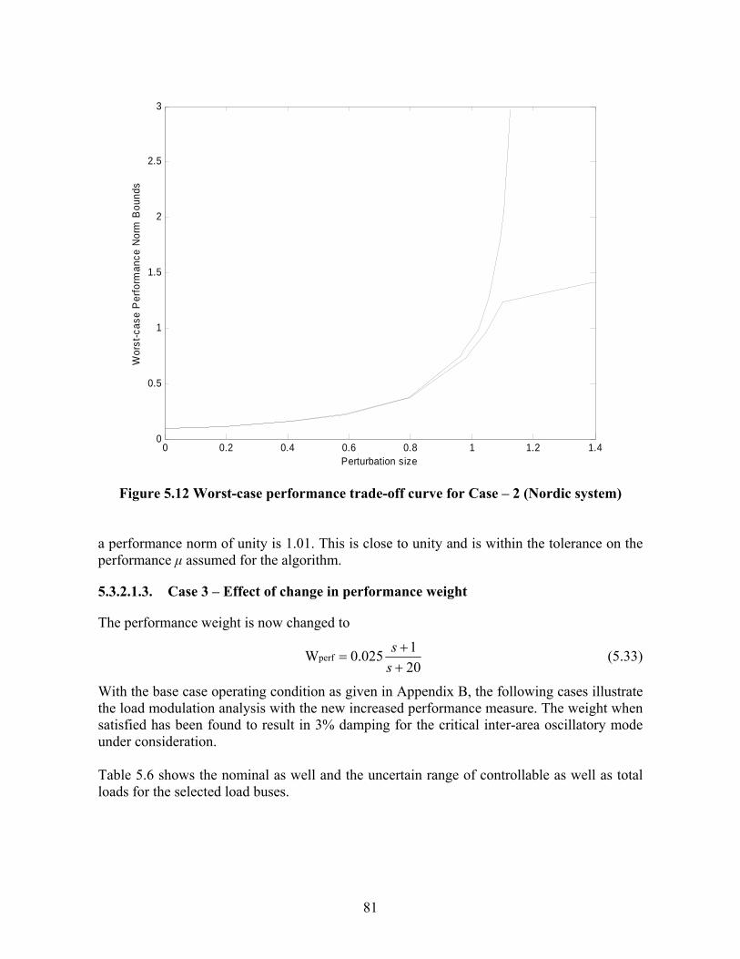
81
Figure 5.12 Worst-case performance trade-off curve for Case – 2 (Nordic system) a performance norm of unity is 1.01. This is close to unity and is within the tolerance on the performance μ assumed for the algorithm.
5.3.2.1.3. Case 3 – Effect of change in performance weight
The performance weight is now changed to
201025.0Wperf
++
=ss (5.33)
With the base case operating condition as given in Appendix B, the following cases illustrate the load modulation analysis with the new increased performance measure. The weight when satisfied has been found to result in 3% damping for the critical inter-area oscillatory mode under consideration. Table 5.6 shows the nominal as well and the uncertain range of controllable as well as total loads for the selected load buses.
0 0.2 0.4 0.6 0.8 1 1.2 1.40
0.5
1
1.5
2
2.5
3
Perturbation size
Wor
st-c
ase
Per
form
ance
Nor
m B
ound
s

82
Table 5.6 Nominal and uncertain load levels for case – 3 (Nordic system)
Bus/Buses Uncontrollable load in MW
Uncertain range of controllable load in MW
Uncertain range of total load in MW
N51 160 [-140 – 140] [20 – 300] N61 70 [-30 – 30] [40 – 190]
S51_1 – S51_5 40 [-15 – 15] [25 – 55] D51_1 – D51_5 20 [-5 – 5] [15 – 25] S61_1 – S61_5 40 [-5 – 5] [35 – 45] D61_1 – D61_5 20 [-5 – 5] [15 – 25]
Corresponding to nominal load levels, the least damped eigenvalue is –0.1287± j3.049. Corresponding to worst-case uncertainty, the least damped eigenvalue is 0.079± j2.383. Thus the system is robustly unstable. The uncertainty levels shown above are scaled to result in the performance μ upper bound being unity (within tolerance εμ = 0.03). Figure 5.13 shows the convergence of performance μ bounds. Table 5.7 shows the resulting maximum uncertainty in load levels that satisfy the chosen damping requirement. It is found that corresponding to these maximum load levels, the least damped eigenvalue is –0.0835± j2.741. The corresponding damping ratio is thus 3.04%.
1 2 31
1.1
1.2
1.3
1.4
1.5
1.6
1.7
Iteration
Per
form
ance
MU
bou
nds
Figure 5.13 Convergence of performance μ bound to unity for Case – 3 (Nordic system)

83
Table 5.7 Maximum uncertainty ranges for controllable and total load levels for Case – 3 (Nordic system)
Load bus/buses Uncontrollable load in MW
Uncertain range of controllable load in MW
Uncertain range of total load in MW
N51 160 [-83.83 – 83.83] [76.17 – 243.83] N61 70 [-17.96 – 17.96] [52.04 – 87.96]
S51_1 – S51_5 40 [-8.98 – 8.98] [31.02 – 48.98] D51_1 – D51_5 20 [-3 – 3] [17 – 23] S61_1 – S61_5 40 [-3 – 3] [37 – 43] D61_1 – D61_5 20 [-3 – 3] [17 – 23]
5.3.2.1.4. Case 4 – Effect of change in performance weight
In this case, both the nominal and uncertainty load levels corresponding to load buses selected for control have been changed as shown in Table 5.8.
Table 5.8 Nominal and uncertain load levels for case – 4 (Nordic system)
Bus/Buses Uncontrollable load in MW
Uncertain range of controllable load in MW
Uncertain range of total load in MW
N51 60 [-40 – 40] [20 – 100] N61 120 [-90 – 90] [30 – 210]
S51_1 – S51_5 40 [-15 – 15] [-25 – 55] D51_1 – D51_5 20 [-5 – 5] [15 – 25] S61_1 – S61_5 40 [-5 – 5] [35 – 45] D61_1 – D61_5 20 [-5 – 5] [15 – 25]
Corresponding to nominal load levels, the least damped eigenvalue is –0.132± j3.101. Corresponding to worst-case uncertainty, the least damped eigenvalue is –0.053± j2.653. In this case, the system is robustly stable. However the chosen performance condition is not satisfied as can be seen from Figure 5.14. The uncertainty levels shown above are scaled to result in the performance μ upper bound being unity (within tolerance εμ = 0.03). Figure 5.14 shows the convergence of performance μ bounds. Table 5.9 shows the resulting maximum uncertainty in load levels that satisfy the chosen damping requirement. It is found that corresponding to these maximum load levels, the least damped eigenvalue is –0.0827± j2.75. The corresponding damping ratio is thus 3%.

84
1 21
1.05
1.1
1.15
Iteration
Per
form
ance
MU
bou
nds
Figure 5.14 Convergence of performance μ bound to unity for Case – 4 (Nordic system)
Table 5.9 Maximum uncertainty ranges for controllable and total load levels for Case – 4 (Nordic system)
Bus/Buses Uncontrollable load in MW
Uncertain range of controllable load in MW
Uncertain range of total load in MW
N51 60 [-34.48 – 34.48] [25.52 – 94.48] N61 120 [-77.59 – 77.59] [42.41 – 197.59]
S51_1 – S51_5 40 [-12.93 – 12.93] [-27.07 – 52.93] D51_1 – D51_5 20 [-4.31 – 4.31] [15.69 – 24.31] S61_1 – S61_5 40 [-4.31 – 4.31] [35.69 – 44.31] D61_1 – D61_5 20 [-4.31 – 4.31] [15.69 – 24.31]
5.3.2.1.5. Small signal stability performance boundary
By a repeated execution of algorithm, explained in Section 5.3, for different nominal and uncertain ranges for the selected loads, different combinations of selected load levels that satisfy the chosen damping performance criterion can be achieved. An explicit boundary of the performance criterion in terms of selected load levels can then be obtained through a least

85
squares curve fit of these different load levels. This is illustrated in the following with an example boundary in terms of loads at 13 KV voltage level: The uncontrollable load levels are as follows: At N51: 210 MW, At N61: 190 MW, At S51_1= S51_2 = S51_3 = S51_4 = S51_5 = 35 MW, At S61_1= S61_2 = S61_3 = S61_4 = S61_5 = 35 MW For the above uncontrollable load levels the following boundary is obtained for loads at D51_1 – D51_5 and D61_1 – D61_5:
)PPPPP(51715.0100 )PPPPP(50953.0
61_561_461_361_261_1
51_551_451_351_2151
++++−=++++_
The accuracy of the boundary is verified as follows: The boundary obtained as above defines the different combination of load levels such that the performance requirement chosen is satisfied within a small tolerance. This is measured by the performance µ being close to 1 within a tolerance, εµ = 0.03. The accuracy of the boundary is demonstrated by choosing arbitrary combinations of load levels that satisfy performance boundary equations and evaluating the performance µ. This has been illustrated for two test cases in the following: Case (i) Let P51_1 = 25 MW, P51_2 = 28 MW, P51_3 = P51_4 = 20 MW, P51_5 = 30 MW and P61_1 = P61_2 = 15 MW. Assuming P61_3 = P61_4 = P61_5, from the performance boundary, P61_3 = P61_4 = P61_5 = 14.06 MW Performance μ upper bound for the above load levels = 1.029 which is within the tolerance εµ. Case (ii) Let P61_1 = 25 MW, P61_2 = 18 MW, P61_3 = 22 MW, P61_4 = 25 MW, P61_5 = 12 MW and P51_1 = P51_2 = P51_3 = 22 MW. Assuming P51_4 = P51_5, from the performance boundary, P51_4 = P51_5 = 13.36 MW Performance μ upper bound for the above load levels = 1.022 which is again within the tolerance assumed.
5.3.2.2 Results on WECC System
The generation and load levels corresponding to the base case operating condition are provided in Appendix C. For this operating condition, there are numerous oscillatory modes observed in the system. However there are three critical oscillatory modes, modes 1, 2 and 3, around frequencies 0.29 Hz, 0.88 Hz and 1.05 Hz respectively, that have been identified and shown in Table 4.3. The participation factors of different machines for these three modes have been shown in Table 4.4. As discussed in Section 4.8.2.1, the error signal that

86
characterizes performance for the above operating condition has been selected as the inertia weighted average of the angular speeds of generators 8, 15, 17, 18 and 22. Tables 5.10 – 5.12 show the real parts of eigenvalue sensitivities corresponding to modes 1, 2 and 3 respectively for different active power loads that are significantly sensitive to the critical modes.
Table 5.10 Significant eigenvalue sensitivities (real-parts) of load buses for Mode 1
Load Bus Eigenvalue sensitivity 2 -0.0093
141 -0.0071 143 -0.0065 145 -0.0064 136 -0.0064 150 -0.0064 50 -0.0064 51 -0.0064 55 -0.0062 109 -0.0055 34 0.0032 31 0.0026 80 0.0014 66 0.0010
Table 5.11 Significant eigenvalue sensitivities (real-parts) of load buses for Mode 2
Load Bus Eigenvalue sensitivity 143 0.0471 51 0.0470 154 0.0469 50 0.0465 55 0.0464 109 0.0455 150 0.0402 41 0.0378 8 0.0307 59 0.0300
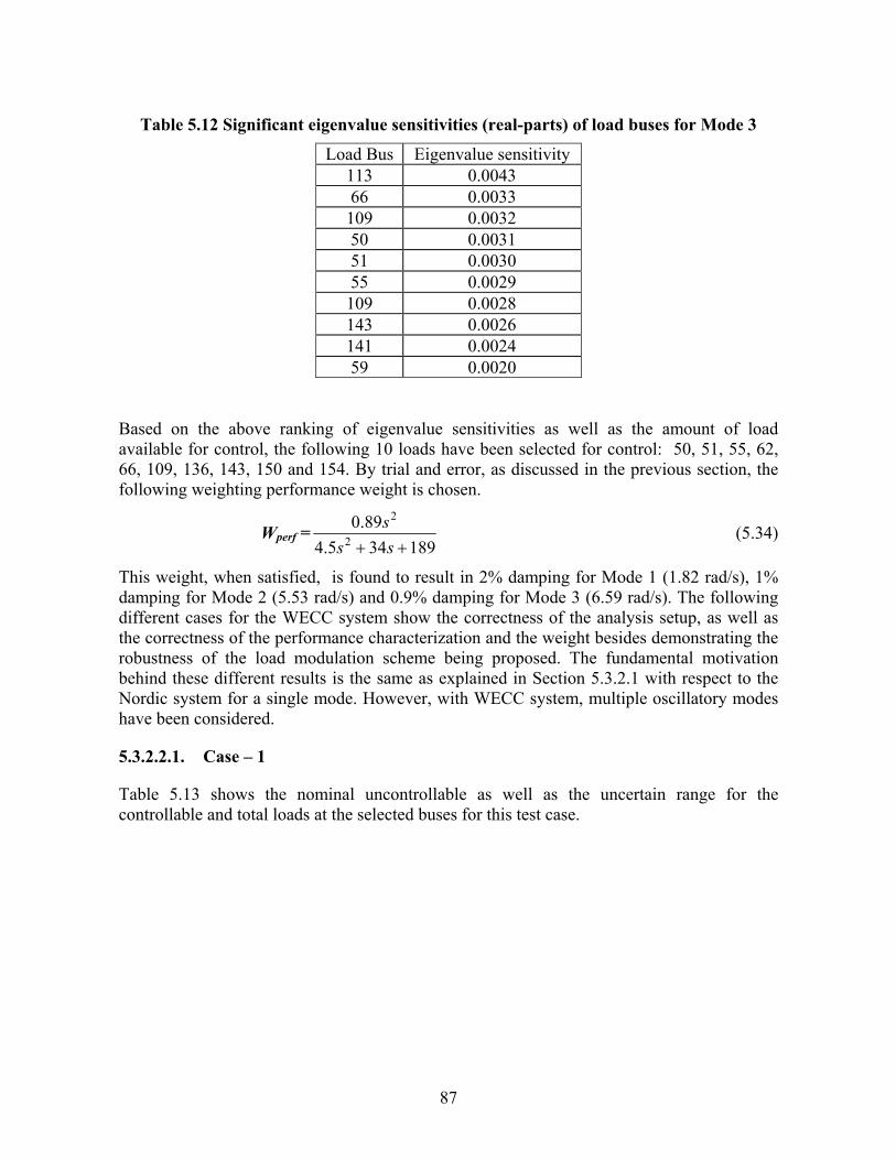
87
Table 5.12 Significant eigenvalue sensitivities (real-parts) of load buses for Mode 3
Load Bus Eigenvalue sensitivity 113 0.0043 66 0.0033 109 0.0032 50 0.0031 51 0.0030 55 0.0029 109 0.0028 143 0.0026 141 0.0024 59 0.0020
Based on the above ranking of eigenvalue sensitivities as well as the amount of load available for control, the following 10 loads have been selected for control: 50, 51, 55, 62, 66, 109, 136, 143, 150 and 154. By trial and error, as discussed in the previous section, the following weighting performance weight is chosen.
Wperf =189345.4
89.02
2
++ sss (5.34)
This weight, when satisfied, is found to result in 2% damping for Mode 1 (1.82 rad/s), 1% damping for Mode 2 (5.53 rad/s) and 0.9% damping for Mode 3 (6.59 rad/s). The following different cases for the WECC system show the correctness of the analysis setup, as well as the correctness of the performance characterization and the weight besides demonstrating the robustness of the load modulation scheme being proposed. The fundamental motivation behind these different results is the same as explained in Section 5.3.2.1 with respect to the Nordic system for a single mode. However, with WECC system, multiple oscillatory modes have been considered.
5.3.2.2.1. Case – 1
Table 5.13 shows the nominal uncontrollable as well as the uncertain range for the controllable and total loads at the selected buses for this test case.

88
Table 5.13 Nominal and uncertain range for selected loads for case – 1 (WECC system)
Bus Uncontrollable load in MW
Uncertain range of controllable load in MW (10% of total load)
Uncertain range of total load in MW
50 1056 [-149.6 – 149.6] [906.4 – 1205.6] 51 397 [-56.23 – 56.23] [340.71 – 453.17] 55 218 [-30.88 – 30.88] [187.06 – 248.81] 62 724.5 [-102.64 – 102.64] [585.63 – 827.13] 66 1104 [-156.4 – 156.4] [947.6 – 1260.4] 109 95.85 [-13.58 – 13.58] [82.27 – 109.42] 136 240.38 [-34.04 – 34.04] [194.31 – 274.44] 143 710 [-100.59 – 100.59] [573.98 – 846.17] 150 2175.6 [-308.2 – 308.2] [1867.3 – 2483.8] 154 1113 [-157.68 – 157.68] [955.35 – 1270.7]
Figure 5.15 shows the performance μ bounds for the above load levels. As can be clearly seen, performance μ peaks above unity to comparable values at the following two frequencies: 1.82 rad/s, and 5.5 rad/s. In addition, performance μ peaks to values less than unity at around 4 rad/s and 6.6 rad/s. There is also a small peak around 3.5 rad/s. Each of the above frequencies corresponds to an oscillatory mode of the system for the above operating conditions. Modes other than the ones with frequencies around 1.8 rad/s (mode 1) and 5.5 rad/s (mode 2) are well-damped for the range of operating conditions for this case. In general, the modes around 4 rad/s and 3.5 rad/s have been found to be well-damped; these are non-critical modes and hence are not considered in subsequent analysis. Clearly for this case, the overall damping performance is not satisfied. Starting with the highest of the peaks of the performance μ upper bound, i.e. 1.39, the uncertainty levels are scaled down until the performance μ upper bound is less than or equal to unity until at each frequency.

89
1 2 3 4 5 6 7 80
0.2
0.4
0.6
0.8
1
1.2
1.4
Frequency in rad/s
Per
form
ance
MU
bou
nds
Figure 5.15 Performance μ bounds for Case – 1 (WECC system)
The convergence of the supremum of performance μ upper bound to unity is shown in Figure 5.16. The peak of the performance μ bound after executing five iterations is shown in Figure 5.17. This peak of unity occurs around 1.8 rad/s. The corresponding load levels are shown in Table 5.14. The critical modes corresponding to the worst-case load levels in the uncertainty range shown above are presented in Table 5.15. Clearly the desired performance is more than satisfied for modes 2 and 3. For mode 1, the desired performance is exactly satisfied as performance μ upper bound is exactly unity at mode 1 frequency. Figure 5.18 shows the response of active power output of generator at bus # 79 for a 50 ms three-phase fault at bus # 44. Mode 1 is clearly the dominant mode that determines the damping performance of the system. Nominal performance is superior than the performance corresponding to worst-case load levels, which as explained in Section 5.3 is a requirement for applying the proposed algorithm.

90
1 2 3 4 5 6 7 80.95
1
1.05
1.1
1.15
1.2
1.25
1.3
1.35
1.4
Iteration
Per
form
ance
MU
bou
nds
Figure 5.16 Convergence of performance μ to unity for case – 1 (WECC system)
1.76 1.77 1.78 1.79 1.8 1.81 1.82 1.83 1.84 1.85 1.860.6
0.65
0.7
0.75
0.8
0.85
0.9
0.95
1
Frequency in rad/s
Per
form
ance
MU
bou
ds
Figure 5.17 Performance μ peak with desired performance satisfied
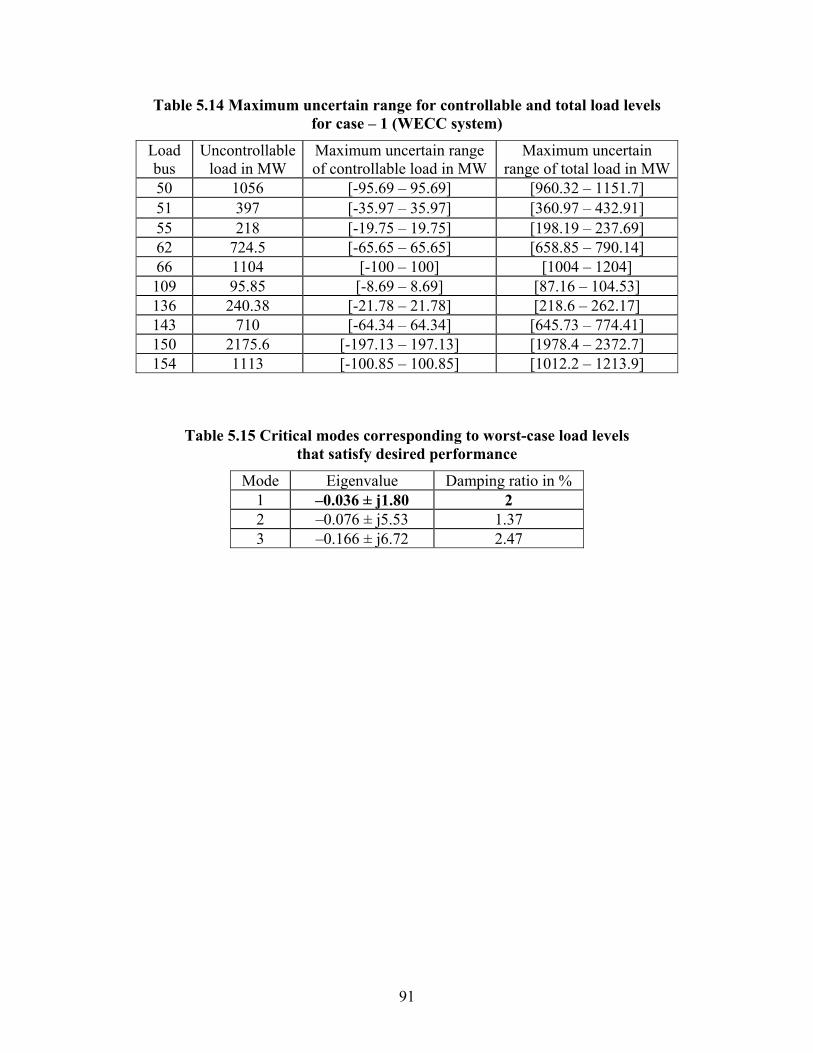
91
Table 5.14 Maximum uncertain range for controllable and total load levels for case – 1 (WECC system)
Load bus
Uncontrollable load in MW
Maximum uncertain range of controllable load in MW
Maximum uncertain range of total load in MW
50 1056 [-95.69 – 95.69] [960.32 – 1151.7] 51 397 [-35.97 – 35.97] [360.97 – 432.91] 55 218 [-19.75 – 19.75] [198.19 – 237.69] 62 724.5 [-65.65 – 65.65] [658.85 – 790.14] 66 1104 [-100 – 100] [1004 – 1204] 109 95.85 [-8.69 – 8.69] [87.16 – 104.53] 136 240.38 [-21.78 – 21.78] [218.6 – 262.17] 143 710 [-64.34 – 64.34] [645.73 – 774.41] 150 2175.6 [-197.13 – 197.13] [1978.4 – 2372.7] 154 1113 [-100.85 – 100.85] [1012.2 – 1213.9]
Table 5.15 Critical modes corresponding to worst-case load levels that satisfy desired performance
Mode Eigenvalue Damping ratio in % 1 –0.036 ± j1.80 2 2 –0.076 ± j5.53 1.37 3 –0.166 ± j6.72 2.47
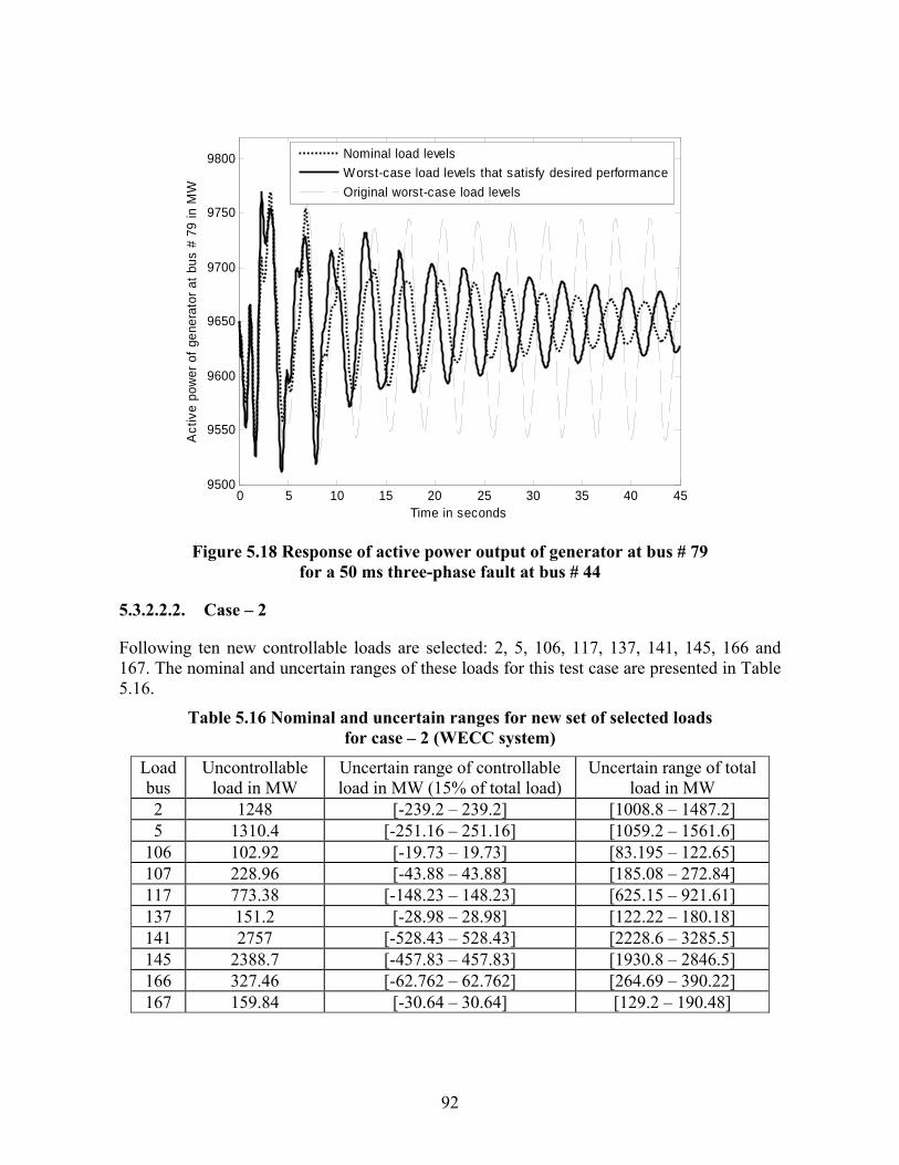
92
0 5 10 15 20 25 30 35 40 459500
9550
9600
9650
9700
9750
9800
Time in seconds
Act
ive
pow
er o
f gen
erat
or a
t bus
# 7
9 in
MW
Nominal load levels Worst-case load levels that satisfy desired performanceOriginal worst-case load levels
Figure 5.18 Response of active power output of generator at bus # 79
for a 50 ms three-phase fault at bus # 44
5.3.2.2.2. Case – 2
Following ten new controllable loads are selected: 2, 5, 106, 117, 137, 141, 145, 166 and 167. The nominal and uncertain ranges of these loads for this test case are presented in Table 5.16.
Table 5.16 Nominal and uncertain ranges for new set of selected loads for case – 2 (WECC system)
Load bus
Uncontrollable load in MW
Uncertain range of controllable load in MW (15% of total load)
Uncertain range of total load in MW
2 1248 [-239.2 – 239.2] [1008.8 – 1487.2] 5 1310.4 [-251.16 – 251.16] [1059.2 – 1561.6]
106 102.92 [-19.73 – 19.73] [83.195 – 122.65] 107 228.96 [-43.88 – 43.88] [185.08 – 272.84] 117 773.38 [-148.23 – 148.23] [625.15 – 921.61] 137 151.2 [-28.98 – 28.98] [122.22 – 180.18] 141 2757 [-528.43 – 528.43] [2228.6 – 3285.5] 145 2388.7 [-457.83 – 457.83] [1930.8 – 2846.5] 166 327.46 [-62.762 – 62.762] [264.69 – 390.22] 167 159.84 [-30.64 – 30.64] [129.2 – 190.48]
93
The generation levels at several buses have also been varied from their base case values as shown in Table 5.17.
Table 5.17 Modified generation levels for case – 2 (WECC system)
Bus Base case generation in MW Modified Generation in MW 6 748 708 65 2210 2610 103 765 465 116 594 294 118 3267 2867 140 3195 3295 144 1290 1190
1.78 1.8 1.82 1.84 1.86 1.88 1.9 1.920.2
0.4
0.6
0.8
1
1.2
1.4
1.6
1.8
2
2.2
Frequency in rad/s
Per
form
ance
MU
bou
nds
Figure 5.19 Performance μ peak around mode 1 frequency for case – 2 (WECC system)

94
5.4 5.42 5.44 5.46 5.48 5.5 5.52 5.54 5.56 5.58 5.60
0.5
1
1.5
2
2.5
Frequency in rad/s
Per
form
ance
MU
bou
nds
Figure 5.20 Performance μ peak around mode 2 frequency for case – 2 (WECC system)
6.2 6.25 6.3 6.35 6.4 6.45 6.5 6.55 6.6 6.65 6.70
0.2
0.4
0.6
0.8
1
1.2
1.4
1.6
Frequency in rad/s
Per
form
ance
MU
bou
nds
Figure 5.21 Performance μ peak around mode 3 frequency for case – 2 (WECC system)

95
Figures 5.19 – 5.21 above show the performance μ peaks around the three critical mode frequencies.
Table 5.18 Maximum uncertain range for controllable and total load levels for case – 2 (WECC system)
Load bus
Uncontrollable load in MW
Maximum uncertain range of controllable load in MW
Maximum uncertain range of total load in MW
2 1248 [-94.02 – 94.02] [1154.98 – 1342.0] 5 1310.4 [-98.72 – 98.72] [1211.7 – 1409.1]
106 102.92 [-7.76 – 7.76] [95.17 – 110.68] 107 228.96 [-17.25 – 17.25] [211.71 – 246.21] 117 773.38 [-58.26 – 58.26] [715.11 – 831.64] 137 151.2 [-11.39 – 11.39] [139.81 – 162.59] 141 2757 [-207.71 – 207.71] [2549.3 – 2964.7] 145 2388.7 [-179.95 – 179.95] [2208.7 – 2568.6] 166 327.46 [-24.67 – 24.67] [302.79 – 352.13] 167 159.84 [-12.04 – 12.04] [147.8 – 171.88]
The final uncertainty range in controllable as well as the total load levels that satisfy the desired performance, obtained through the application of the proposed algorithm are presented in Table 5.18. Figure 5.22 below presents the convergence of performance μ bound to unity (within tolerance) in arriving at the load levels shown in Table 5.18.
1 2 3 4 5 61
1.5
2
2.5
Iteration
Per
form
ance
MU
bou
nds
Figure 5.22 Convergence of performance μ to unity for case – 2 (WECC system)

96
The performance μ bounds corresponding to the load levels that satisfy the desired damping performance are shown in Figure 5.23. The performance μ bounds reach unity around mode 1 frequency. For the initial uncertainty, mode 2 is the dominant mode. That is, the damping performance corresponding to the worst-case load levels in the initial uncertainty shown in Table 5.16 is dominated by mode 2, with frequency around 5.5 rad/s. However, the damping performance in the new scaled down uncertainty, obtained through the application of the algorithm is dominated by mode 1. This can also be verified through non-linear simulation results shown in Figure 5.24. The response for the initial load levels is dominated by mode 2 (unstable), whereas for the new scaled uncertainty, the response is dominated by mode 1 (with 2% damping). The critical modes corresponding to the worst-case load levels in the above uncertainty range are shown in Table 5.24. Clearly the desired performance is satisfied for modes 1, 2 and 3.
1.78 1.8 1.82 1.84 1.86 1.88 1.9 1.92
0.4
0.5
0.6
0.7
0.8
0.9
1
1.1
Frequency in rad/s
Per
form
ance
MU
bou
nds
Figure 5.23 Performance μ peak with desired performance satisfied
Table 5.19 Critical modes corresponding to worst-case load levels that satisfy desired performance
Mode Eigenvalue Damping ratio in % 1 –0.037 ± j1.84 2.01 2 –0.097 ± j5.54 1.75 3 –0.155 ± j6.73 2.3
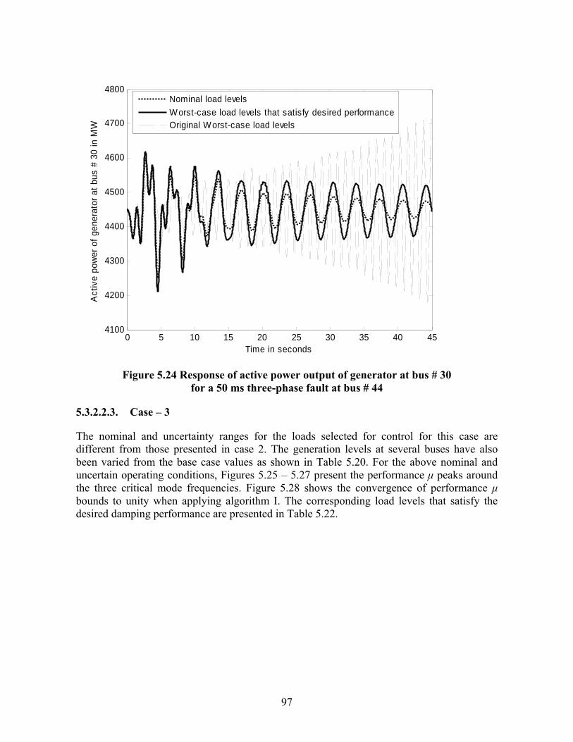
97
0 5 10 15 20 25 30 35 40 454100
4200
4300
4400
4500
4600
4700
4800
Time in seconds
Act
ive
pow
er o
f gen
erat
or a
t bus
# 3
0 in
MW
Nominal load levelsWorst-case load levels that satisfy desired performanceOriginal Worst-case load levels
Figure 5.24 Response of active power output of generator at bus # 30
for a 50 ms three-phase fault at bus # 44
5.3.2.2.3. Case – 3
The nominal and uncertainty ranges for the loads selected for control for this case are different from those presented in case 2. The generation levels at several buses have also been varied from the base case values as shown in Table 5.20. For the above nominal and uncertain operating conditions, Figures 5.25 – 5.27 present the performance μ peaks around the three critical mode frequencies. Figure 5.28 shows the convergence of performance μ bounds to unity when applying algorithm I. The corresponding load levels that satisfy the desired damping performance are presented in Table 5.22.
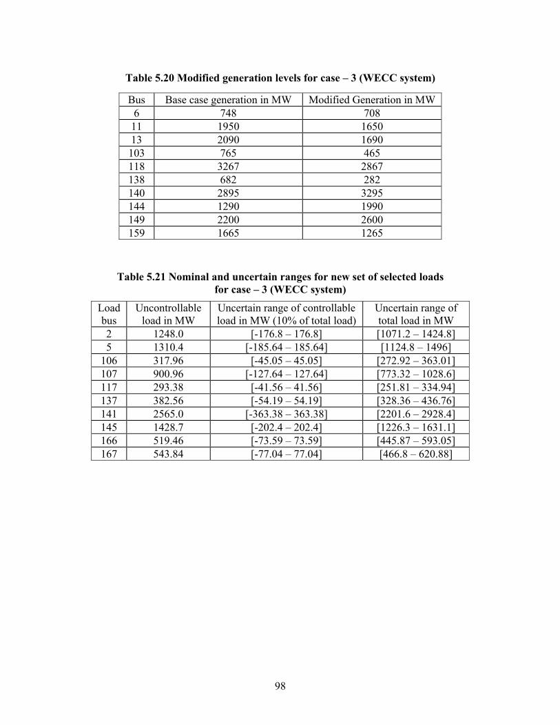
98
Table 5.20 Modified generation levels for case – 3 (WECC system)
Table 5.21 Nominal and uncertain ranges for new set of selected loads for case – 3 (WECC system)
Load bus
Uncontrollable load in MW
Uncertain range of controllable load in MW (10% of total load)
Uncertain range of total load in MW
2 1248.0 [-176.8 – 176.8] [1071.2 – 1424.8] 5 1310.4 [-185.64 – 185.64] [1124.8 – 1496]
106 317.96 [-45.05 – 45.05] [272.92 – 363.01] 107 900.96 [-127.64 – 127.64] [773.32 – 1028.6] 117 293.38 [-41.56 – 41.56] [251.81 – 334.94] 137 382.56 [-54.19 – 54.19] [328.36 – 436.76] 141 2565.0 [-363.38 – 363.38] [2201.6 – 2928.4] 145 1428.7 [-202.4 – 202.4] [1226.3 – 1631.1] 166 519.46 [-73.59 – 73.59] [445.87 – 593.05] 167 543.84 [-77.04 – 77.04] [466.8 – 620.88]
Bus Base case generation in MW Modified Generation in MW 6 748 708 11 1950 1650 13 2090 1690 103 765 465 118 3267 2867 138 682 282 140 2895 3295 144 1290 1990 149 2200 2600 159 1665 1265
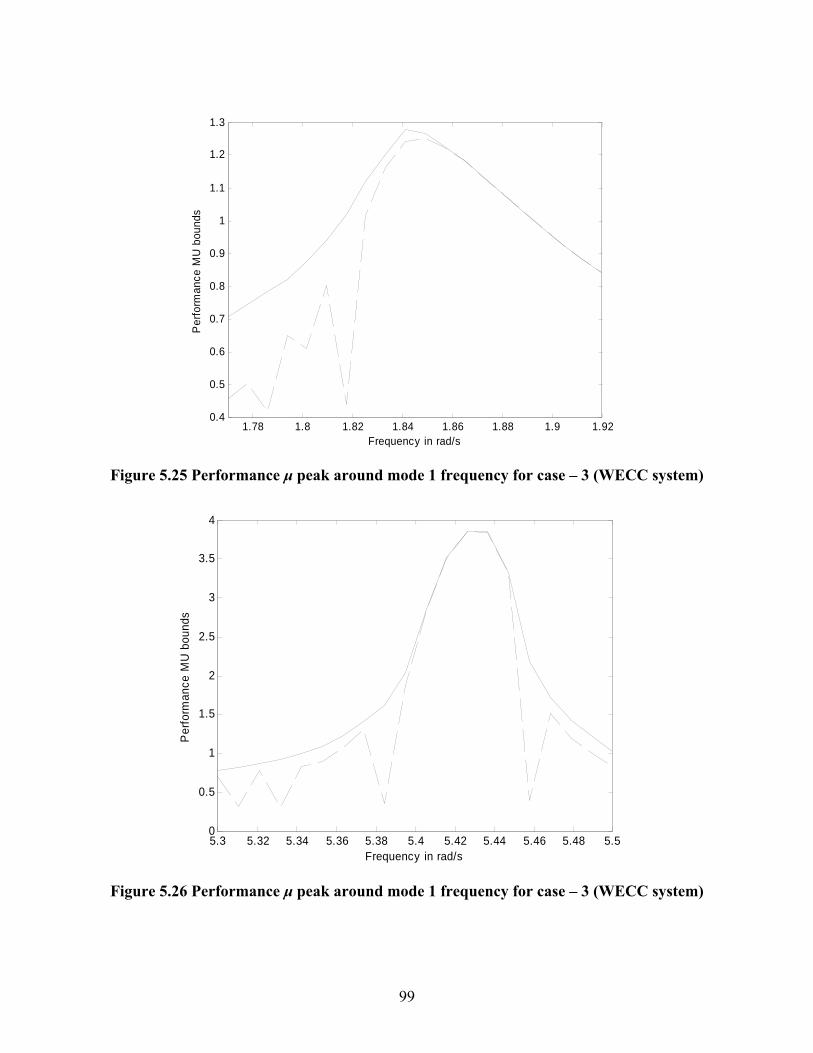
99
1.78 1.8 1.82 1.84 1.86 1.88 1.9 1.920.4
0.5
0.6
0.7
0.8
0.9
1
1.1
1.2
1.3
Frequency in rad/s
Per
form
ance
MU
bou
nds
Figure 5.25 Performance μ peak around mode 1 frequency for case – 3 (WECC system)
5.3 5.32 5.34 5.36 5.38 5.4 5.42 5.44 5.46 5.48 5.50
0.5
1
1.5
2
2.5
3
3.5
4
Frequency in rad/s
Per
form
ance
MU
bou
nds
Figure 5.26 Performance μ peak around mode 1 frequency for case – 3 (WECC system)

100
6.3 6.35 6.4 6.45 6.5 6.55 6.60
0.2
0.4
0.6
0.8
1
1.2
1.4
1.6
1.8
Frequency in rad/s
Per
form
ance
MU
bou
nds
Figure 5.27 Performance μ peak around mode 3 frequency for case – 3 (WECC system)
1 2 3 4 5 6 7 80
0.5
1
1.5
2
2.5
3
3.5
4
Iteration
Per
form
ance
MU
bou
nds
Figure 5.28 Convergence of performance μ to unity for case – 3 (WECC system)
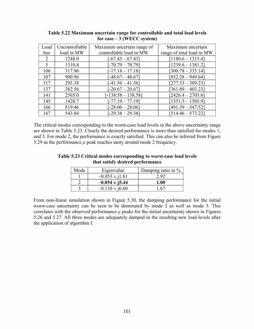
101
Table 5.22 Maximum uncertain range for controllable and total load levels for case – 3 (WECC system)
Load bus
Uncontrollable load in MW
Maximum uncertain range of controllable load in MW
Maximum uncertain range of total load in MW
2 1248.0 [-67.43 – 67.43] [1180.6 – 1315.4] 5 1310.4 [-70.79 – 70.79] [1239.6 – 1381.2]
106 317.96 [-17.18 – 17.18] [300.78 – 335.14] 107 900.96 [-48.67 – 48.67] [852.28 – 949.64] 117 293.38 [-41.56 – 41.56] [277.53 – 309.23] 137 382.56 [-20.67 – 20.67] [361.89 – 403.23] 141 2565.0 [-138.58 – 138.58] [2426.4 – 2703.6] 145 1428.7 [-77.19 – 77.19] [1351.5 – 1505.9] 166 519.46 [-28.06 – 28.06] [491.39 – 547.52] 167 543.84 [-29.38 – 29.38] [514.46 – 573.22]
The critical modes corresponding to the worst-case load levels in the above uncertainty range are shown in Table 5.23. Clearly the desired performance is more than satisfied for modes 1, and 3. For mode 2, the performance is exactly satisfied. This can also be inferred from Figure 5.29 as the performance μ peak reaches unity around mode 2 frequency.
Table 5.23 Critical modes corresponding to worst-case load levels that satisfy desired performance
Mode Eigenvalue Damping ratio in % 1 –0.053 ± j1.81 2.92 2 –0.054 ± j5.44 1.00 3 –0.110 ± j6.60 1.67
From non-linear simulation shown in Figure 5.30, the damping performance for the initial worst-case uncertainty can be seen to be dominated by mode 2 as well as mode 3. This correlates with the observed performance μ peaks for the initial uncertainty shown in Figures 5.26 and 5.27. All three modes are adequately damped in the resulting new load levels after the application of algorithm I.

102
Figure 5.29 Performance μ peak with desired performance satisfied
0 5 10 15 20 25 309610
9615
9620
9625
9630
9635
9640
9645
9650
9655
9660
Time in seconds
Act
ive
pow
er o
f gen
erat
or a
t bus
# 7
9 in
MW
Nominal load levelsWorst-case load levels that satisfy desired performanceOriginal waorst-case load levels
Figure 5.30 Response of generator at bus # 79 for a 50 ms three-phase fault at bus # 44
5.35 5.4 5.45 5.5 5.55 0.5
0.6
0.7
0.8
0.9
1
1.1
1.2
Frequency in rad/s
Perfo
rman
ce M
U b
ound
s

103
5.4 Approach II – Determination of Worst-case Performance for Fixed Uncertainty
The following are three fundamental aspects with respect to Approach II:
i) Uncertainty could exist in load levels, generation levels or in any parameter of the system model.
ii) The system is required to satisfy the chosen performance specifications over the range of the uncertainty.
iii) Load modulation is performed based on sensitivities of critical eigenvalues to controllable active power loads.
iv) Different loads have different sensitivities to the critical eigenvalues and these sensitivities vary over operating conditions. The result is that the above load modulation process is iterative. It is performed until the worst-case performance satisfies the desired specifications.
To determine the worst-case performance for a given uncertainty, the magnitude of the perturbations Δ in Δ defined in (5.11) is kept fixed ( )1)( ≤Δσ . That is, in the N–∆ setup, the skewed – μ of N is evaluated by varying just the performance part of N. That is achieved by
defining ⎥⎦
⎤⎢⎣
⎡=
IkI
Kn
n 00
and iterating on kn until μ = 1.
1
Δ0Δ)det( :Δ)(min:)(
−
∈⎟⎠
⎞⎜⎝
⎛== NI-KNK nXn σμ
κκ (5.35)
The worst-case performance for a given uncertainty thus obtained is then compared against the desired performance specification. Load modulation is resorted to in case the desired performance is not satisfied. The fundamental premise behind load modulation in this approach is a strong correlation observed between the performance μ upper bound peaking frequencies and the critical mode frequencies. For example, this has been demonstrated in Figures 5.6, and 5.10 for the Nordic system and Figures 5.15, 5.19 – 5.21, and 5.25 – 5.27 for the WECC system. Thus by modulating loads to improve the damping performance of each of the critical modes individually, the overall system desired damping performance could be achieved. Eigenvalue sensitivities corresponding to each critical mode from different active power loads are used as indices to perform load modulation. Depending on the participation of different generators in each of the critical oscillatory modes, as well as depending on the power flow pattern corresponding to system operating condition, the eigenvalue sensitivities of different loads vary both in magnitude and sign. Also these sensitivities vary with changes in operating conditions. Thus as loads are modulated, these sensitivities need to be reevaluated and further modulation of loads will have to be performed based on the updated sensitivities. The result is that the overall load modulation process is iterative.

104
5.4.1 Algorithm for Approach II
Following is the algorithm for Approach II – Determination of Worst-case performance for fixed uncertainty. Given the uncertainty in load, generation or any physical parameter, form a reasonably dense grid of operating points in terms of the uncertainty. It has been verified that consideration of three points (minimum, nominal, and maximum) in the uncertainty range is sufficient.
i) Execute power flows corresponding to different combinations of minimum, nominal and maximum operating points in the uncertainty range.
ii) Form the linear model (A and B matrices) for each operating point in the grid. iii) Calculate linear curve-fitting coefficients for each varying element of the A and B
matrices, to be expressed in terms of the underlying uncertainties. iv) Express the uncertain system in N-Δ framework for robust performance analysis
by characterizing the uncertainty in LFT form and characterizing performance through weighted error signals, as explained in section 4.8.
v) Calculate the worst-case performance for the above uncertainty. If desired performance is not satisfied, then execute (a) – (d) below followed by repetition of steps (i) – (v), else stop. a. Calculate eigenvalue sensitivities for different controllable active power loads.
The sign of the real-part of the sensitivity is used to decide an increase or decrease of load at the bus for improving the damping performance.
b. For each critical oscillatory mode, rank the loads in the increasing order of the magnitude of the real-parts of the eigenvalue sensitivities.
c. Select the number of loads to be modulated for each critical mode. d. Perform load modulation based on the ranking obtained in step (b) for the
above selected loads.

105
Figure 5.31 Flowchart of the algorithm for approach II – Determination of worst-case
performance for given uncertainty
5.4.2 Approach II – Numerical Simulations and Results
Generation levels corresponding generators at buses 140 and 144 are assumed to be uncertain. The uncertainty range has been assumed to be 8% of the nominal generation levels in each of the following cases. In each of the following cases, similar to the results shown for Approach I, the nominal load as well as the generation levels have been varied drastically. It has then been shown that when loads are modulated to satisfy the performance μ bound to
Stop
Calculate Eigenvalue
sensitivities for different
controllable active
Execute Powerflows corresponding to different combinations of minimum,
nominal and maximum operating points in the
uncertainty range
Form A and B matrices for the different operating points
considered in the previous step
Calculate linear curve-fitting coefficients for each varying
element of the A and B matrices
Express the system in N-Δ framework through uncertainty representation in LFT form and performance characterization
Start
Uncertainty in load,
generation, or any
physical parameter
Calculate worst-case performance using
skewed μUB
Rank load buses according to their
sensitivities for critical modes
Select load buses for control
implementation from the ranking
Perform load modulation at the
selected buses based on
Eigenvalue
Desired performance
satisfied?
Yes
No

106
unity, the desired performance is exactly satisfied for each of these different cases. The correctness of the algorithm as well as the robustness of the approach is thereby demonstrated.
5.4.2.1 Approach II – Case 1
The nominal load and generation levels corresponding to this test case is shown in Appendix C. The uncertainties in generation levels are shown in Table 5.24.
Table 5.24 Uncertainty in generation at bus # 140 and bus # 144 for case 1 – Approach II (WECC system)
Bus Nominal generation in MW Uncertainty in generation levels in MW140 3195 [2939.4 – 3450.6] 144 1290 [1186.8 – 1393.2]
For the above nominal operating condition and uncertainty ranges, in addition to modes 1, 2 and 3 identified earlier, two other oscillatory modes with frequencies around 3.4 rad/s and 4.7 rad/s have been observed. All modes except mode 1 are sufficiently damped over the range of operating conditions. The error signal characterizing performance has been chosen as the inertia weighted average of the angular speeds of generators 8, 15, 17, 18 and 22, by following the procedure explained in Section 4.8. By trial and error, the following weighting function is chosen:
Wperf = 189216
73.02
2
++ sss . The above weight, when satisfied, has been verified to result in a
damping ratio of 2% for mode 1 which is the critical mode for this case. As can be verified from Figure 5.32, for the above nominal operating point and the uncertainty ranges, mode 1 is determinant of the overall damping performance of the system.

107
1 2 3 4 5 6 7 80
0.5
1
1.5
2
2.5
3
3.5
4
4.5
Frequency in rad/s
Per
form
ance
MU
bou
nds
Figure 5.32 Performance μ bounds for case 1 – Approach II (WECC system)
Table 5.25 Load buses with high eigenvalue sensitivities (real-parts) for Mode 1
Bus Eigenvalue sensitivity (real parts) 5 -0.0122 2 -0.0083 17 -0.0062 10 -0.0059 8 -0.0058 16 -0.0038 19 -0.0038 12 -0.0036 136 -0.0031 139 -0.0029 141 -0.0027 152 -0.0026 164 -0.0024 143 -0.0024 51 -0.0023
For the nominal operating condition, Table 5.25 above shows the load buses that have the highest eigenvalue sensitivities for mode 1.
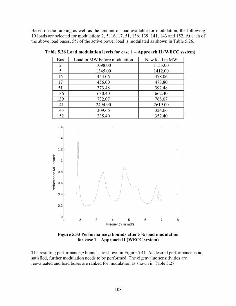
108
Based on the ranking as well as the amount of load available for modulation, the following 10 loads are selected for modulation: 2, 5, 16, 17, 51, 136, 139, 141, 143 and 152. At each of the above load buses, 5% of the active power load is modulated as shown in Table 5.26.
Table 5.26 Load modulation levels for case 1 – Approach II (WECC system)
Bus Load in MW before modulation New load in MW 2 1098.00 1153.00 5 1345.00 1412.00 16 454.06 478.06 17 456.00 478.80 51 373.48 392.48 136 630.40 662.40 139 732.07 768.07 141 2494.90 2619.00 143 309.66 324.66 152 335.40 352.40
1 2 3 4 5 6 7 80
0.2
0.4
0.6
0.8
1
1.2
1.4
1.6
Frequency in rad/s
Per
form
ance
MU
bou
nds
Figure 5.33 Performance μ bounds after 5% load modulation
for case 1 – Approach II (WECC system) The resulting performance μ bounds are shown in Figure 5.41. As desired performance is not satisfied, further modulation needs to be performed. The eigenvalue sensitivities are reevaluated and load buses are ranked for modulation as shown in Table 5.27.
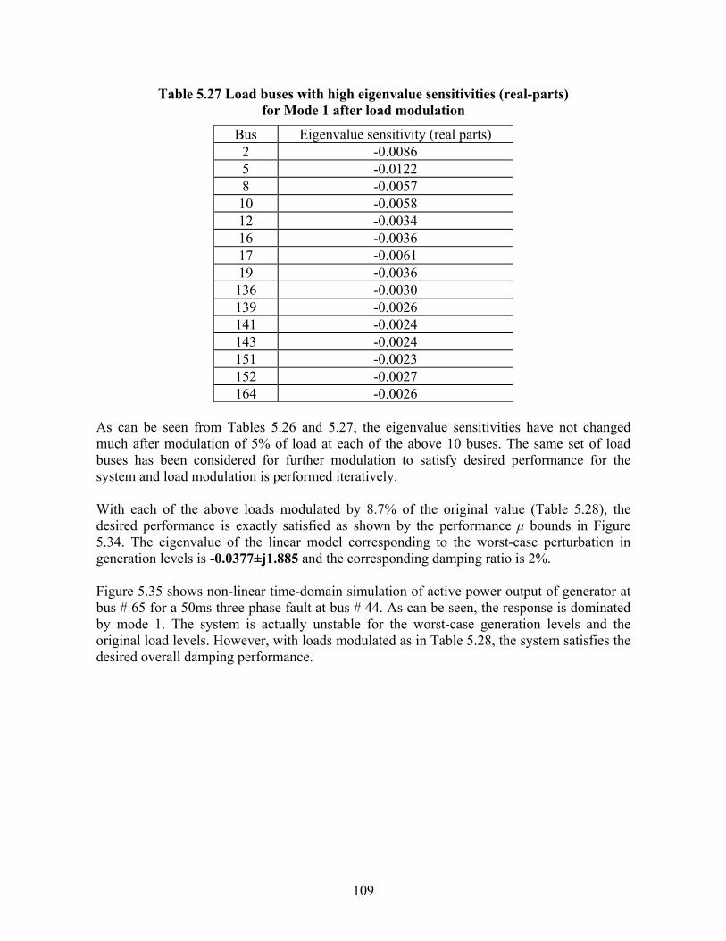
109
Table 5.27 Load buses with high eigenvalue sensitivities (real-parts) for Mode 1 after load modulation
Bus Eigenvalue sensitivity (real parts) 2 -0.0086 5 -0.0122 8 -0.0057 10 -0.0058 12 -0.0034 16 -0.0036 17 -0.0061 19 -0.0036 136 -0.0030 139 -0.0026 141 -0.0024 143 -0.0024 151 -0.0023 152 -0.0027 164 -0.0026
As can be seen from Tables 5.26 and 5.27, the eigenvalue sensitivities have not changed much after modulation of 5% of load at each of the above 10 buses. The same set of load buses has been considered for further modulation to satisfy desired performance for the system and load modulation is performed iteratively. With each of the above loads modulated by 8.7% of the original value (Table 5.28), the desired performance is exactly satisfied as shown by the performance μ bounds in Figure 5.34. The eigenvalue of the linear model corresponding to the worst-case perturbation in generation levels is -0.0377±j1.885 and the corresponding damping ratio is 2%. Figure 5.35 shows non-linear time-domain simulation of active power output of generator at bus # 65 for a 50ms three phase fault at bus # 44. As can be seen, the response is dominated by mode 1. The system is actually unstable for the worst-case generation levels and the original load levels. However, with loads modulated as in Table 5.28, the system satisfies the desired overall damping performance.

110
Table 5.28 Load levels that satisfy chosen performance for case 1 – Approach II (WECC system)
Bus Load in MW before modulation
Final load levels after modulation in MW
2 1098.00 1193.50 5 1345.00 1463 16 456.00 496 17 454.06 494 51 373.48 406 136 630.40 685.25 139 732.07 796.07 141 2494.90 2712 143 309.66 336.6 152 335.40 365
1 2 3 4 5 6 7 80
0.1
0.2
0.3
0.4
0.5
0.6
0.7
0.8
0.9
1
Frequency in rad/s
Per
form
ance
MU
bou
nds
Figure 5.34 Performance μ bounds with desired performance exactly satisfied
for case 1 – Approach II (WECC system)
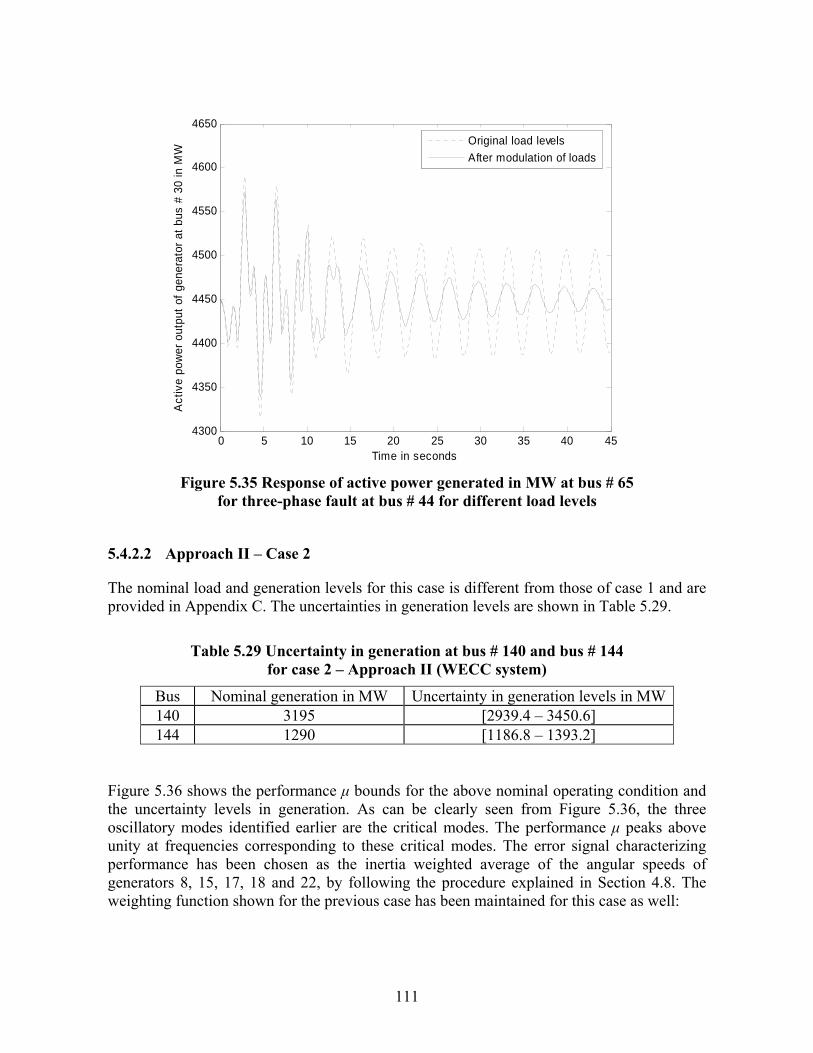
111
0 5 10 15 20 25 30 35 40 454300
4350
4400
4450
4500
4550
4600
4650
Time in seconds
Act
ive
pow
er o
utpu
t of g
ener
ator
at b
us #
30
in M
W
Original load levelsAfter modulation of loads
Figure 5.35 Response of active power generated in MW at bus # 65
for three-phase fault at bus # 44 for different load levels
5.4.2.2 Approach II – Case 2
The nominal load and generation levels for this case is different from those of case 1 and are provided in Appendix C. The uncertainties in generation levels are shown in Table 5.29.
Table 5.29 Uncertainty in generation at bus # 140 and bus # 144 for case 2 – Approach II (WECC system)
Bus Nominal generation in MW Uncertainty in generation levels in MW140 3195 [2939.4 – 3450.6] 144 1290 [1186.8 – 1393.2]
Figure 5.36 shows the performance μ bounds for the above nominal operating condition and the uncertainty levels in generation. As can be clearly seen from Figure 5.36, the three oscillatory modes identified earlier are the critical modes. The performance μ peaks above unity at frequencies corresponding to these critical modes. The error signal characterizing performance has been chosen as the inertia weighted average of the angular speeds of generators 8, 15, 17, 18 and 22, by following the procedure explained in Section 4.8. The weighting function shown for the previous case has been maintained for this case as well:

112
Wperf = 189216
73.02
2
++ sss
1 2 3 4 5 6 7 80
0.5
1
1.5
2
2.5
Frequency in rad/s
Per
form
ance
MU
bou
nds
Figure 5.36 Performance μ bounds for case 2 – Approach II (WECC system)
Tables 5.30 – 5.32 below present the ranking of eigenvalue sensitivities of different loads for each of the critical modes.

113
Table 5.30 Ranking of loads based on eigenvalue sensitivities for mode 1
Bus Eigenvalue sensitivity (real parts) 5 -0.0302 2 -0.0111 17 -0.0097 10 -0.0092 8 -0.0091
164 -0.0071 12 -0.0048 19 -0.0047 16 -0.0047 136 -0.0040 158 -0.0039 139 -0.0039 166 -0.0037 44 -0.0037 152 -0.0035
Table 5.31 Ranking of loads based on eigenvalue sensitivities for mode 2
Bus Eigenvalue sensitivity (real parts) 50 0.0180 51 0.0177 54 0.0177 57 0.0176 58 0.0176 41 0.0176 143 0.0174 141 0.0172 55 0.0172 62 0.0172 137 0.0172 150 0.0171 154 0.0171 145 0.0171 48 0.0170
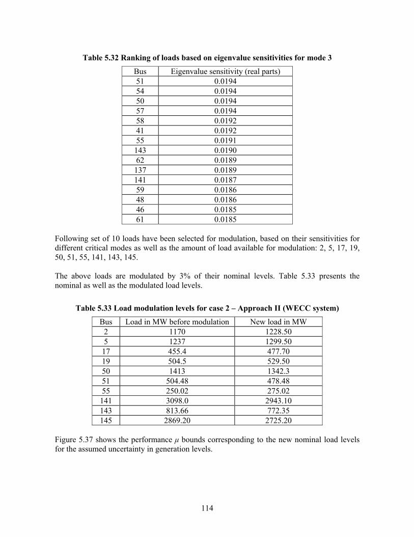
114
Table 5.32 Ranking of loads based on eigenvalue sensitivities for mode 3
Bus Eigenvalue sensitivity (real parts) 51 0.0194 54 0.0194 50 0.0194 57 0.0194 58 0.0192 41 0.0192 55 0.0191 143 0.0190 62 0.0189 137 0.0189 141 0.0187 59 0.0186 48 0.0186 46 0.0185 61 0.0185
Following set of 10 loads have been selected for modulation, based on their sensitivities for different critical modes as well as the amount of load available for modulation: 2, 5, 17, 19, 50, 51, 55, 141, 143, 145. The above loads are modulated by 3% of their nominal levels. Table 5.33 presents the nominal as well as the modulated load levels.
Table 5.33 Load modulation levels for case 2 – Approach II (WECC system)
Bus Load in MW before modulation New load in MW 2 1170 1228.50 5 1237 1299.50 17 455.4 477.70 19 504.5 529.50 50 1413 1342.3 51 504.48 478.48 55 250.02 275.02 141 3098.0 2943.10 143 813.66 772.35 145 2869.20 2725.20
Figure 5.37 shows the performance μ bounds corresponding to the new nominal load levels for the assumed uncertainty in generation levels.

115
As can be seen, the desired performance is not satisfied. Load modulation is performed iteratively and the desired performance specifications have been found to be satisfied through modulation of 5.9% of the original nominal load levels for each of the above loads.
1 2 3 4 5 6 7 80
0.2
0.4
0.6
0.8
1
1.2
1.4
Frequency in rad/s
Per
form
ance
MU
bou
nds
Figure 5.37 Performance μ bounds after 3% load modulation
for case 2 – Approach II (WECC system) Table 5.34 presents the final modulated load levels for which the desired performance is satisfied. Figure 5.38 shows the corresponding performance μ bounds, and as can be seen, desired performance is exactly satisfied. Table 5.35 shows the eigenvalues of the linear model corresponding to the worst-case perturbation in generation for the new load levels after modulation. The desired performance requirement corresponding to modes 1 and 2 are exactly satisfied. This is also verified through non-linear time domain simulation for different load levels presented in Figure 5.39. The response can be seen to be comprised of the dynamics of modes 1 and 2.
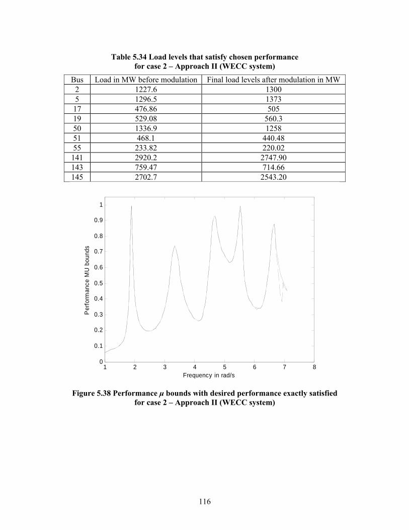
116
Table 5.34 Load levels that satisfy chosen performance for case 2 – Approach II (WECC system)
Bus Load in MW before modulation Final load levels after modulation in MW 2 1227.6 1300 5 1296.5 1373 17 476.86 505 19 529.08 560.3 50 1336.9 1258 51 468.1 440.48 55 233.82 220.02 141 2920.2 2747.90 143 759.47 714.66 145 2702.7 2543.20
1 2 3 4 5 6 7 80
0.1
0.2
0.3
0.4
0.5
0.6
0.7
0.8
0.9
1
Frequency in rad/s
Per
form
ance
MU
bou
nds
Figure 5.38 Performance μ bounds with desired performance exactly satisfied
for case 2 – Approach II (WECC system)

117
Table 5.35 Critical modes corresponding to worst-case generation levels in uncertainty range after load modulation
Mode Eigenvalue Damping ratio in % 1 –0.0378 ± j1.89 2.00 2 –0.0554 ± j5.54 1.00 3 –0.0793 ± j6.61 1.19
0 5 10 15 20 25 30 35 40 452140
2160
2180
2200
2220
2240
2260
2280
Time in seconds
Act
ive
pow
er o
utpu
t of g
ener
ator
at b
us #
65
in M
W
Original load levelsAfter modulation of loads
Figure 5.39 Response of active power generated in MW at bus # 65
for three-phase fault at bus # 44 for different load levels
5.4.2.3 Approach II – Case 3
The nominal generation and load levels for this case are different from those of cases 1 and 2 presented above and are provided in Appendix C. The uncertainties in generation levels are shown in Table 5.36.

118
Table 5.36 Uncertainty in generation at bus # 140 and bus # 144 for case 3 – Approach II (WECC system)
Bus Nominal generation in MW Uncertainty in generation levels in MW140 2895 [2663.4 – 3126.6] 144 1690 [1554.8 – 1825.2]
Figure 5.40 shows the performance μ bounds for the above nominal operating condition and the uncertainty levels in generation.
1 2 3 4 5 6 7 80
0.2
0.4
0.6
0.8
1
1.2
1.4
1.6
1.8
Frequency in rad/s
Per
form
ance
MU
bou
nds
Figure 5.40 Performance μ bounds for case 3 – Approach II (WECC system)
As can be seen, the performance μ peaks above unity at frequencies corresponding to the three critical modes around 1.8 rad/s and 5.5 rad/s and 6.7 rad/s respectively. The same performance error signal and the weight considered in previous cases have been maintained for this case as well. Tables 5.37 – 5.39 below present the loads that exhibit high eigenvalue sensitivities for critical modes and the corresponding eigenvalue sensitivities.

119
Table 5.37 Ranking of loads based on eigenvalue sensitivities for mode 1
Bus Eigenvalue sensitivity (real parts) 5 -0.0279 2 -0.0109 17 -0.0092 10 -0.0087 8 -0.0086
164 -0.0067 19 -0.0047 12 -0.0047 16 -0.0047 136 -0.0040 139 -0.0039 152 -0.0035 34 -0.0034 158 -0.0032 141 -0.0031
Table 5.38 Ranking of loads based on eigenvalue sensitivities for mode 2
Bus Eigenvalue sensitivity (real parts) 51 0.0181 141 0.0180 54 0.0180 143 0.0179 50 0.0179 57 0.0179 58 0.0179 41 0.0179 154 0.0178 137 0.0178 55 0.0177 109 0.0176 150 0.0176 62 0.0175 59 0.0175
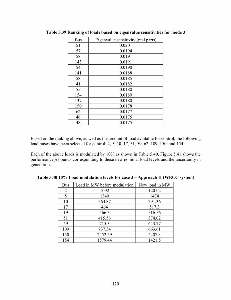
120
Table 5.39 Ranking of loads based on eigenvalue sensitivities for mode 3
Bus Eigenvalue sensitivity (real parts) 51 0.0201 57 0.0194 58 0.0191 143 0.0191 54 0.0190 141 0.0188 58 0.0185 41 0.0182 55 0.0180 154 0.0180 137 0.0180 150 0.0178 62 0.0177 46 0.0175 48 0.0175
Based on the ranking above, as well as the amount of load available for control, the following load buses have been selected for control: 2, 5, 10, 17, 51, 59, 62, 109, 150, and 154. Each of the above loads is modulated by 10% as shown in Table 5.40. Figure 5.41 shows the performance μ bounds corresponding to these new nominal load levels and the uncertainty in generation.
Table 5.40 10% Load modulation levels for case 3 – Approach II (WECC system)
Bus Load in MW before modulation New load in MW 2 1092 1201.2 5 1340 1474 10 264.87 291.36 17 464 517.3 19 466.3 516.56 51 415.58 374.02 59 715.3 643.77 109 737.34 663.61 150 2452.59 2207.3 154 1579.44 1421.5

121
1 2 3 4 5 6 7 80
0.1
0.2
0.3
0.4
0.5
0.6
0.7
0.8
0.9
1
Frequency in rad/s
Per
form
ance
MU
bou
nds
Figure 5.41 Performance μ bounds after 10% modulation of loads
for case 3 – Approach II (WECC system) As can be seen from Figure 5.41, with 10% of each of the above loads modulated, the desired performance is more than satisfied. However, when each of the above loads is iteratively modulated to 7.6% as shown in Table 5.46, the desired performance is exactly satisfied for both modes 1 and 2. This can be inferred from the performance μ bounds shown in Figure 5.50. The critical eigenvalues corresponding to worst-case generation perturbations after load modulation is shown in Table 5.42. Performance requirement corresponding to modes 1 and 2 are exactly satisfied. As can be seen from the non-linear simulation for a 50 ms three-phase fault at bus # 44 in Figure 5.43, the response of the system corresponding to worst-case uncertainty after load modulation is dominated by all three modes of oscillations.
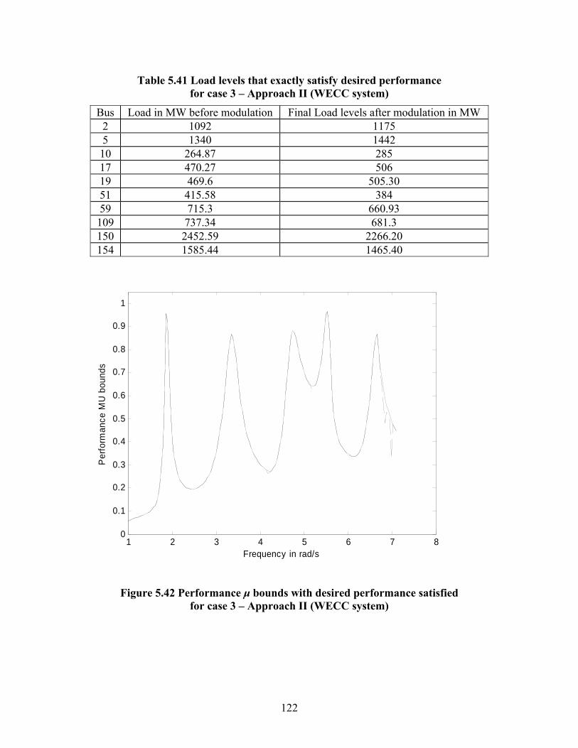
122
Table 5.41 Load levels that exactly satisfy desired performance for case 3 – Approach II (WECC system)
Bus Load in MW before modulation Final Load levels after modulation in MW 2 1092 1175 5 1340 1442 10 264.87 285 17 470.27 506 19 469.6 505.30 51 415.58 384 59 715.3 660.93 109 737.34 681.3 150 2452.59 2266.20 154 1585.44 1465.40
1 2 3 4 5 6 7 80
0.1
0.2
0.3
0.4
0.5
0.6
0.7
0.8
0.9
1
Frequency in rad/s
Per
form
ance
MU
bou
nds
Figure 5.42 Performance μ bounds with desired performance satisfied for case 3 – Approach II (WECC system)

123
Table 5.42 Critical eigenvalues corresponding to worst-case generation levels after load modulation for case 3 – Approach II (WECC system)
Mode Eigenvalue Damping ratio in %
1 –0.0377 ± j1.88 2.01 2 –0.0556 ± j5.55 1.00 3 –0.0763 ± j6.61 1.15
0 5 10 15 20 25 30 35 40 452160
2170
2180
2190
2200
2210
2220
2230
2240
2250
2260
Time in seconds
Act
ive
pow
er o
utpu
t of g
ener
ator
at b
us #
65
in M
W
After modulation of loadOriginal load levels
Figure 5.43 Response of active power generated in MW at bus # 65
for three-phase fault at bus # 44 for different load levels

124
6. Load Control Algorithms
This section deals in detail with different algorithms for real-time modulation of loads. Having obtained the load levels that satisfy the desired damping performance, either as a performance load level boundary or as the total amount of load to be modulated at the transmission level, the problem of modulating different types of loads over a period of time in order to satisfy the above load level requirement is addressed in this section. Specialized algorithms have been developed for different types of loads for real-time load modulation. In developing these algorithms, certain recent developments in enabling technologies such as load control systems and communication infrastructure have been taken into account. This section starts with a brief background of these recent developments and the impact of these developments on load control programs. An optimization framework for performing Monte Carlo simulations for the study of load control is then developed. Two Dynamic Programming-based algorithms and a decision-tree based algorithm for air-conditioner and water-heater loads have been developed for this study. A variety of results that demonstrate the impact of different types of constraints in the algorithms as well as different parameters in the model have been presented.
6.1 Background
6.1.1 Brief Historical Overview of Load Control Technology
For many years, utilities have developed load management programs for the commercial and industrial sectors. More recently, utility as well as ISO interest has focused on the potential of demand response in the residential and small commercial sector. Residential demand for heating and cooling tends to be the major contributor to system peaks. These sectors are more capable of reducing their loads—by bigger amounts and with more flexibility—than large commercial customers. At the same time, as the interest in demand response for the residential and small commercial sectors grew, a few manufacturers have made impressive strides in metering and load control technologies in the residential and small commercial sectors. These new developments enable the utility to maintain a continuous two-way communication with its customers' appliances, in real time. These developments facilitate consideration of several newer objectives in load management programs besides the ones traditionally considered. As discussed in the literature survey in Section 2, traditional objectives in load management programs have been two fold: Improvement of economics of operation and improvement of reliability through peak load management. In considering these objectives, very little attention was given to customer discomfort. This could be attributed to the non-availability of economically viable technology to implement distributed load control with minimum disruption. The first generation of load control, executed in 80’s and early 90’s was one-way: during a crisis, the utility would shut off customer equipments to lower demand. The second generation of load control was improved, utilizing controllable thermostats, but it was still

125
one-way. However, in one-way systems, because of the possibility of overriding the control from utility by the customer, the amount of load controlled was always more than necessary. This suboptimal as well as disruptive form of direct load control often created considerable discontent.
6.1.2 Telecommunications Reform Act of 1996
In the first and second generation of load control, utilities relied mostly on their own power distribution infrastructure. This was because utilities did not have rights to other communication modes. The most appealing technology was power line carrier communication. Ripple control by means of radio links and radio receivers was another popular technology. In both these technologies, bandwidth, i.e. speed and detail of information capability, is limited and two-way communication, although possible, is very complicated. Thus there were very few two-way communication systems between utilities and customers with the exception of some large (mostly industrial) customers. In 1996, the telecommunications reform act was passed to encourage competition in all aspects of telecommunication services and carriers. This was a landmark legislation in the telecommunication sector and it provided utilities the rights to other modes of communication. This paved the way for cost-effective technologies for two-way communication with customer sites. Fiber-optic system, data cable, which is a hybrid fiber-optic and coaxial cable system, phone lines for high-speed data transfer, cellular phone systems, paging systems, are some of the different communication systems that are being considered today for direct load control technology.
6.1.3 Developments in Load Control Systems
Breakthroughs in communication and sensor technologies and the drive for energy efficiency have resulted in the availability of programmable thermostats. These are thermostats that combine a communication module with a conventional setback thermostat. Using the communications module, the host energy provider can raise or lower the thermostat to impact device operations. Several manufacturers have recently begun offering this new generation of technology in space-heating equipments. The prevailing level of interest in two-way communicating “smart thermostat” products is quite substantial and growing. A half dozen thermostat suppliers are now vying to participate in this market, prominent among them are United Technologies’ Carrier, Honeywell, Invensys, Comverge Technologies, White Rodgers etc. Figure 6.1 shows a screen shot of Carrier’s Emi thermostat applied in some of the recent pilot programs. This is a two-way communication enabled thermostat whose settings can be accessed over the internet by the utility as well as the customer. At any point of time during the control period, the customer can override the utility control either directly or remotely through the internet. The utility can monitor the Emi responses and the customer overrides. The customer can access or program the thermostat through the web interface and the utility when cycling the air-conditioners would try to adhere to customer setting.

126
Figure 6.1 Screenshot of Carrier’s Emi thermostat
Figure 6.2 shows a screenshot of another popular thermostat, ExpressStatTM, a product of an alliance between Cannon Technologies and Honeywell. Motorola FLEX paging is underlying the communication technology.
Figure 6.2 Screenshot of Honeywell’s ExpressStat® air-conditioner

127
6.1.4 Some Recent Applications of the Above Technologies
6.1.4.1 LIPAedge Program
The Long Island Power Authority (LIPA) is completing its third year of LIPA Edge (http://www.lipaedge.com), the largest residential and small commercial direct load control (DLC) program in the United States using a two-way communications system. There are over 25,000 participants, of which 3,200 are small commercial accounts. Carrier’s Emi thermostat was applied on Itron’s communication platform, the overall system called ComfortChoiceTM. The system offers some unique features, combining all the functions of a programmable thermostat with the ability of customers to control their thermostats over the internet. LIPAEdge was originally started in the summer of 2002 as a pilot program to test the feasibility of supplying spinning reserves using responsive loads on “critical” days when the import of power into Long Island was severely limited.
6.1.4.2 Myappliance.com Program
MyAppliance.com is the first system in the industry to offer web-enabled and WAP (Wireless Application Protocol) phone technology enabled air-conditioning (http://www.myappliance.com). Beginning with a pilot program to be offered this summer in Europe, this "smart" air conditioner is equipped with a wireless communication device that enables real-time two-way communication. Any service technician can also communicate with the equipment via a hand held device or desktop computer. For the end-user, the service-oriented, interactive web feature allows connected users access to the controls of their air conditioning equipment.
6.1.4.3 Automated Demand Response Systems (ADRS) – Invensys GoodWatts
This new load management technology, known individually as automated demand response systems (ADRS) solves many of the problems that limited the older generation of load control. ADRS continuously control the temperature of the home within the comfort zone defined by the customer, and provide the utility with real-time on load reduction, so just the right number of homes are controlled. Invensys's GoodWatts technology—a system whereby homeowners and their utilities can communicate with and remotely control major home appliances via the Internet—combines clear market signals and efficiency to add reliability to local and regional grids, as well as to shave off unnecessary kilowatts for consumers (http://www.invensysnetworks.com). GoodWatts is a sophisticated home energy management system that employs an "always on" broadband connection to allow utilities and customers to engage in two-way communications to automatically control a customer's home energy loads in real time. This system has been successfully applied recently at PECO Energy in Pennsylvania, Nevada Power, and all three major California utilities. Today’s technology allows finer and more discrete control of several distributed loads almost in real-time. The possibility of cost-effective, continuous two-way communication with the end-user resources allows consideration of customer discomfort when executing control. It is possible to minimize the discomfort caused as a result of control through effective cycling of
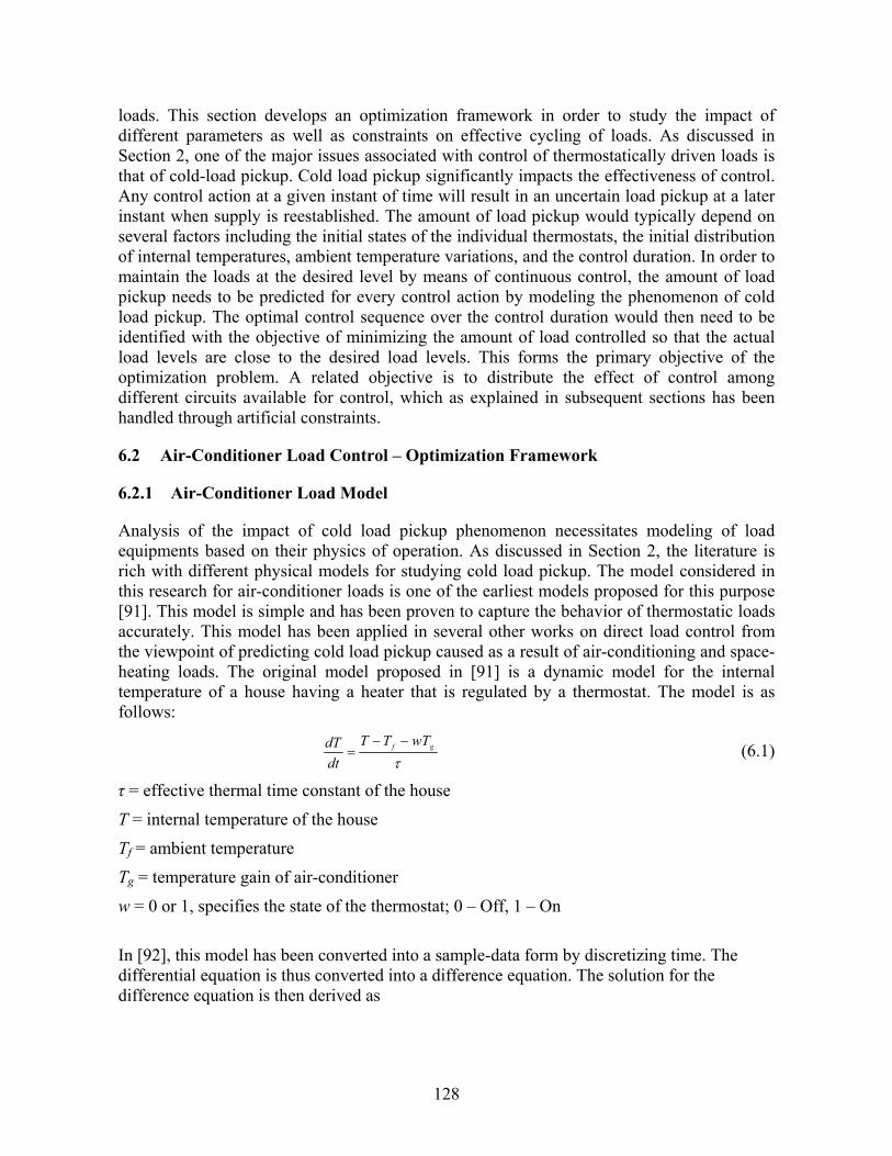
128
loads. This section develops an optimization framework in order to study the impact of different parameters as well as constraints on effective cycling of loads. As discussed in Section 2, one of the major issues associated with control of thermostatically driven loads is that of cold-load pickup. Cold load pickup significantly impacts the effectiveness of control. Any control action at a given instant of time will result in an uncertain load pickup at a later instant when supply is reestablished. The amount of load pickup would typically depend on several factors including the initial states of the individual thermostats, the initial distribution of internal temperatures, ambient temperature variations, and the control duration. In order to maintain the loads at the desired level by means of continuous control, the amount of load pickup needs to be predicted for every control action by modeling the phenomenon of cold load pickup. The optimal control sequence over the control duration would then need to be identified with the objective of minimizing the amount of load controlled so that the actual load levels are close to the desired load levels. This forms the primary objective of the optimization problem. A related objective is to distribute the effect of control among different circuits available for control, which as explained in subsequent sections has been handled through artificial constraints.
6.2 Air-Conditioner Load Control – Optimization Framework
6.2.1 Air-Conditioner Load Model
Analysis of the impact of cold load pickup phenomenon necessitates modeling of load equipments based on their physics of operation. As discussed in Section 2, the literature is rich with different physical models for studying cold load pickup. The model considered in this research for air-conditioner loads is one of the earliest models proposed for this purpose [91]. This model is simple and has been proven to capture the behavior of thermostatic loads accurately. This model has been applied in several other works on direct load control from the viewpoint of predicting cold load pickup caused as a result of air-conditioning and space-heating loads. The original model proposed in [91] is a dynamic model for the internal temperature of a house having a heater that is regulated by a thermostat. The model is as follows:
τgf wTTT
dtdT −−
= (6.1)
τ = effective thermal time constant of the house
T = internal temperature of the house
Tf = ambient temperature
Tg = temperature gain of air-conditioner
w = 0 or 1, specifies the state of the thermostat; 0 – Off, 1 – On
In [92], this model has been converted into a sample-data form by discretizing time. The differential equation is thus converted into a difference equation. The solution for the difference equation is then derived as
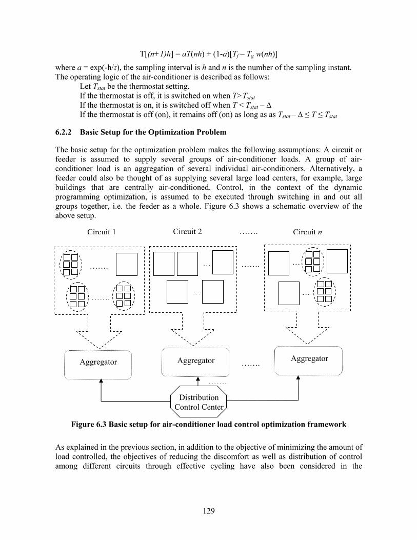
129
T[(n+1)h] = aT(nh) + (1-a)[Tf – Tg w(nh)]
where a = exp(-h/τ), the sampling interval is h and n is the number of the sampling instant. The operating logic of the air-conditioner is described as follows:
Let Tstat be the thermostat setting. If the thermostat is off, it is switched on when T>Tstat If the thermostat is on, it is switched off when T < Tstat – Δ If the thermostat is off (on), it remains off (on) as long as as Tstat – ∆ ≤ T ≤ Tstat
6.2.2 Basic Setup for the Optimization Problem
The basic setup for the optimization problem makes the following assumptions: A circuit or feeder is assumed to supply several groups of air-conditioner loads. A group of air-conditioner load is an aggregation of several individual air-conditioners. Alternatively, a feeder could also be thought of as supplying several large load centers, for example, large buildings that are centrally air-conditioned. Control, in the context of the dynamic programming optimization, is assumed to be executed through switching in and out all groups together, i.e. the feeder as a whole. Figure 6.3 shows a schematic overview of the above setup.
Figure 6.3 Basic setup for air-conditioner load control optimization framework
As explained in the previous section, in addition to the objective of minimizing the amount of load controlled, the objectives of reducing the discomfort as well as distribution of control among different circuits through effective cycling have also been considered in the
……. … …….
……. …
…
…
Aggregator Aggregator Aggregator
Distribution Control Center
…….
…….
Circuit 1 Circuit 2 Circuit n…….

130
optimization problem. It is possible to minimize the amount of load controlled by causing severe discomfort. In this case effective cycling of the controllable loads is not performed and hence the need for these additional objectives.
6.2.3 Dynamic Programming-Based Optimization Objective
The primary objective of the optimization problem is to minimize the deviation of the actual total load from the desired load levels.
Minimize destimektime
N
iuk PPP
itime
feeders
itime ,1
,,−+∑ ∑
=
(6.2)
whereitimeukP
,and
itimekP,
are the uncontrollable load and controllable air-conditioner load in
feeder i at the time interval under consideration, and destimeP , is the desired load level. Nfeeders is the total number of feeders available for control.
6.2.4 Dynamic Programming-Based Optimization Constraints
In addition to the primary objective, it is also desired to distribute the effect of control effectively amongst different circuits available for control, that is, to minimize the difference between total absolute mean temperature excursions from thermostat set-points between different circuits.
Minimize ∑ ∑∑≠ ==
−ji
N
kkj
N
ki
jgig
kTT
11ΔΔ ; i, j =1,…., Nfeeders (6.3)
wherekiTΔ is the temperature deviation of group k in feeder i from the mean thermostat set-
point of the group and Ngi is the number of groups of air-conditioner loads being supplied by feeder i. However, the above objective cannot be directly dealt with in the optimization problem. This is on account of the difficulty in the availability of telemetered data such as internal temperatures as well as thermostat set-points that are essential in modeling the objective in the optimization problem. The approach taken is to add artificial constraints that indirectly deal with the objective of distributing the effect of control. Two different artificial constraints have been tried in the following algorithms:
A) Maximum off-time and minimum on-time constraint B) Constraint on temperature excursion
6.2.4.1 Maximum off-time and minimum on-time constraints
6.2.4.1.1. Maximum off-time constraint
A circuit is assumed to supply several air-conditioner loads. Once a circuit is switched off either through on/off control or through coordinated thermostat set-point control, resulting in

131
all air-conditioners supplied by that circuit being turned off, the circuit is not allowed to remain off beyond a pre-specified duration, called the maximum off-time.
6.2.4.1.2. Minimum on-time constraint
Once a circuit that had earlier been switched off for load control is switched on, it should remain on; i.e., the air-conditioners are allowed to operate under natural cycling for at least the duration of the minimum on-time specified a priori before it can be considered for control again.
6.2.4.2 Constraint on temperature excursion
Each circuit has a pre-specified maximum average internal temperature excursion, which if exceeded, the circuit is switched on if it was off through coordinated thermostat set-point control. Once on, the air-conditioners are allowed to operate under natural cycling until the average internal temperature excursions decrease below the threshold. No constraint is imposed on the switching times in this case. The maximum average internal temperature excursion is the average of the individual temperature excursions of different groups of air-conditioners supplied by the circuit. A similar approach towards effective cycling of air-conditioners has been attempted in the LIPAEdge program discussed earlier. To contrast the above two constraints, in the former the temperature excursion is controlled indirectly through the control of on and off times of load circuits. The total number and times of disruption is a measure of discomfort. In the latter, the temperature excursions are controlled directly. Conceptually, both these constraints attempt effective cycling among the different circuits of loads available for control.
6.2.5 Dynamic Programming Algorithm Parameters
A strategy in the DP is the combination of on/off states of different circuits. The DP algorithm parameters given in (Figure 6.4) include:
a) Number of strategies to search for each time instant (q) b) Number of strategies to store for each time instant (qsi) c) Time period considered for direct load control

132
6.2.6 Assumption of Uncertainties for Monte Carlo Simulations
In the results that are presented in this section, the Monte Carlo simulation is extensively applied in analyzing the effect of different parameters as well as constraints in the load control algorithms. This strategy has been adopted from the viewpoint of generating test scenarios that approximate realistic operating conditions. By assuming uncertainties in different model parameters and external variables that closely resemble real-life operating conditions, Monte Carlo simulations are performed through repeated sampling of uncertain variables. This repeated sampling generates several test cases within the uncertainty ranges. The algorithms are tested for each of the above cases. Their success rates in finding feasible solutions thus enable drawing conclusions about the overall operating scenario. The results of these Monte Carlo simulations also enable analyzing the effect of different parameters and variables on the overall effect of control. For the purpose of Monte Carlo simulations, uncertainties have been assumed in the following parameters and variables:
i) Initial internal temperature distribution for the air-conditioners in each circuit available for control
ii) Thermostat set-point distribution for air-conditioners iii) Air-conditioner parameters – a, Tg, τ, Δ – these generate diversity among air-
conditioner equipments available for control; the amount of uncertainties could be altered thereby reflecting closely real-life scenarios
All the above uncertainties introduce diversity in the duty cycles of air-conditioners available for control.
6.2.7 Initialization of Scenario
In order to introduce diversity in the duty cycles of air-conditioners, the initial inside temperatures and thermostat set-points for different groups of air-conditioner for optimization problem are initialized with pre-specified probability distributions. The above scenario is simulated without load control for a sufficiently long duration so that the initial dynamics settle down and the air-conditioners enter their natural cycling [91]. This is illustrated in Figure 6.5 with the following parameters:
Number of groups of air-conditioners (or large air-conditioner loads) = 10000
Initial internal temperatures: Normal distribution with mean = 72 F and standard deviation = 12 F, i.e. N(72,12)
Air-conditioner model parameters: τ – N(64, 5), Tg = N(30,10)
Thermostat set-point: N(72,4)
Ambient temperature variation: 1 to 100 min – 80 F and 101 to 160 min – 85 F

133
Figure 6.4 Dynamic Programming solution parameters
As can be seen from the following simulation in Figure 6.5, the air-conditioners when initialized with the above parameters enter into natural cycling after 60 minutes as can be inferred from the distribution of the internal temperatures shown in Figure 6.5. The scenario corresponding to 60 minutes is then used as the initial scenario for the DP based optimization problem.
.
.
.
.
.
.
.
.
.
.
.
.
State 1
State 2
State k M
State k+1
State k+2 M
State 2k
.
.
.
.
.
.
.
.
State q
Interval n Interval n+1
Stored State 1
Stored State 2
Stored State m+1
Stored State qs n+1

134
20 30 40 50 60 70 80 90 100 110 1200
500
1000
1500
2000
2500
3000
Internal temperature in Fahrenheit
Num
ber o
f air-
cond
ition
ers
Distribution at t=0Distribution at t=20 minDistribution at t=60 min Distribution at t=80 min
Figure 6.5 Simulation of internal temperature distributions
6.2.8 Small-Signal Stability Performance Boundary
The proposed algorithms for load control at distribution level of the system have been illustrated using the small-signal performance boundary obtained in Section 5.3.2.1.5 for the augmented Nordic system reproduced below:
)PPPPP(51715.0100 )PPPPP(50953.0
61_561_461_361_261_1
51_551_451_351_2151
++++−=++++_
This boundary has been obtained for the Nordic system augmented with 10 distribution feeders with a damping requirement of 2 % for the least damped inter-area mode in the system. As explained in the results for this boundary in Section 5.3.2.1.5, as long as the load levels in the different feeders are maintained such that the boundary is exactly satisfied, the overall system damping would at least be 2% ± 0.03%; 0.03% was the tolerance assumed in deriving the above boundary. It is to be noted that the proposed algorithms could also be applied for analyzing load modulation performed only at the transmission level of the system. In this case, the amount of load modulation obtained at the transmission level load buses would actually be modulated at the distribution level among available feeders through the application of the proposed algorithms.

135
6.2.9 Monte Carlo Simulation Results with On/Off Time Constraints
The data shown below correspond to the operating conditions assumed for the optimization problem: Number of feeders = 10 (corresponding to D51_1 – D51_5 and D61_1 – D61_5 in Figure 5.5 of the augmented Nordic system)
Number of groups of air-conditioners in each feeder = 100
Rating of each group = 120 KW
Total maximum controllable load in each feeder = 12 MW
Uncontrollable load in each feeder = 13.6 MW
Initial internal temperatures: Normal distribution N(79,12)
Air-conditioner model parameters: τ – N(64, 10), Tg = N(30,5)
Thermostat set-point: N(72,4); Δ = 1.5 F
Ambient temperature variation: 1 to 100 min – 89 F ; 101 to 150 min – 95 F;
151 to 200 min – 90 F; 201 to 250 min – 85 F
0 50 100 150 200 25080
82
84
86
88
90
92
94
96
98
100
Time in minutes
Am
bien
t tem
pera
ture
in F
ahre
nhei
t
Figure 6.6 Assumed variation of ambient temperature

136
0 50 100 150 200 250-10
-5
0
5
10
15
20
25
30
35
Time in minutes
Per
form
ance
bou
ndar
y vi
olat
ion
in M
W
Figure 6.7 Desired small-signal stability performance boundary violation
with no load control Performance boundary considered is the boundary obtained for the Nordic system in Section 5.3.2.1.5.
)PPPPP(51715.0100 )PPPPP(50953.0
61_561_461_361_261_1
51_551_451_351_2151
++++−=++++_
DP algorithm parameters: Number of strategies to search at each time instant – 128 Number of strategies to store at each time instant – 3 In all of the following results, the scenario corresponding to 50 minutes is used as the initial scenario for the DP-based optimization algorithm. For the above operating conditions, the air-conditioner cycling in all circuits is simulated, and thereby the total air-conditioner load levels are calculated at each time instant. This is essentially a very short-term load forecast considering only air-conditioner loads. The performance boundary violation is then evaluated using the total load levels at each time instant. This is shown in Figure 6.7. The desired performance boundary is continuously violated for the above operating conditions, thereby resulting in inferior damping performance. Thus, load modulation needs to be performed in order to satisfy desired damping specifications as defined by the performance boundary.

137
6.2.9.1 Effect of cycling time constraints on the effectiveness of control
Maximum off time =4 minutes; Minimum on time = 2 minutes Figure 6.8 shows representative Monte Carlo simulation results of performance boundary violation for the above case. As can be seen from Figure 6.8, the load levels that result from the DP based optimization algorithm are close to the desired performance boundary and there is no violation of the desired load levels defined by the boundary at any time instant for the above operating conditions and algorithm constraints. However, as these constraints are made more stringent by reducing the difference between maximum off-time and minimum on-time, the algorithm fails to find feasible solutions that satisfy the constraints, as shown in Section 6.2.7.2.
0 50 100 1500
24
68
10
-4
-3.5
-3
-2.5
-2
-1.5
-1
-0.5
0
Time in minutes
Number of runs
Per
form
ance
bou
ndar
y vi
olat
ion
in M
W
Figure 6.8 Monte Carlo simulation results for maximum off-time – 4 min,
minimum on-time – 2 min
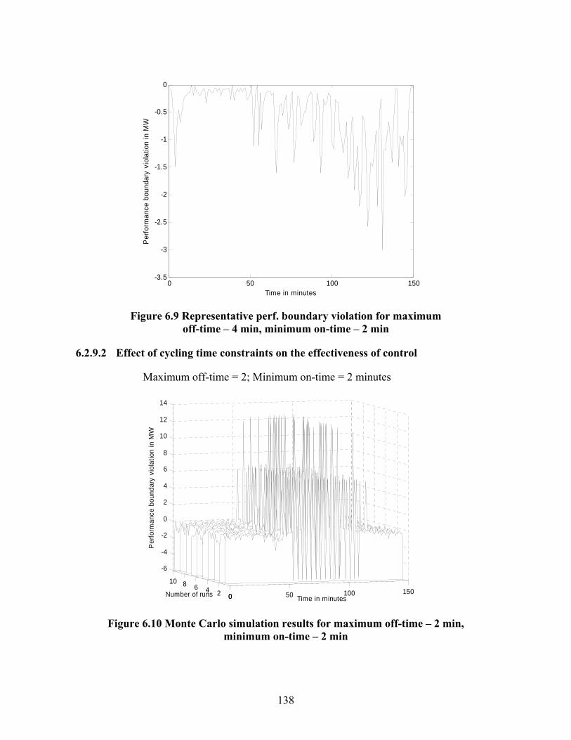
138
0 50 100 150-3.5
-3
-2.5
-2
-1.5
-1
-0.5
0
Time in minutes
Per
form
ance
bou
ndar
y vi
olat
ion
in M
W
Figure 6.9 Representative perf. boundary violation for maximum
off-time – 4 min, minimum on-time – 2 min
6.2.9.2 Effect of cycling time constraints on the effectiveness of control
Maximum off-time = 2; Minimum on-time = 2 minutes
0 50 100 1500246810
-6
-4
-2
0
2
4
6
8
10
12
14
Time in minutesNumber of runs
Per
form
ance
bou
ndar
y vi
olat
ion
in M
W
Figure 6.10 Monte Carlo simulation results for maximum off-time – 2 min,
minimum on-time – 2 min
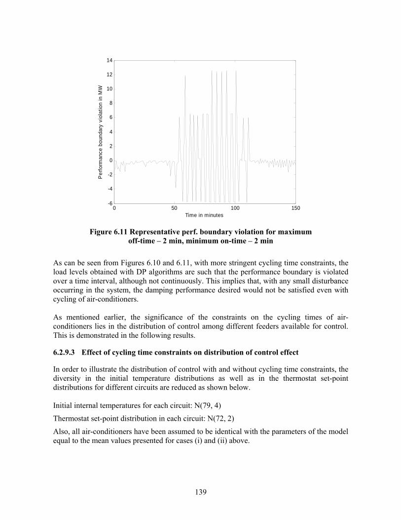
139
0 50 100 150-6
-4
-2
0
2
4
6
8
10
12
14
Time in minutes
Per
form
ance
bou
ndar
y vi
olat
ion
in M
W
Figure 6.11 Representative perf. boundary violation for maximum
off-time – 2 min, minimum on-time – 2 min As can be seen from Figures 6.10 and 6.11, with more stringent cycling time constraints, the load levels obtained with DP algorithms are such that the performance boundary is violated over a time interval, although not continuously. This implies that, with any small disturbance occurring in the system, the damping performance desired would not be satisfied even with cycling of air-conditioners. As mentioned earlier, the significance of the constraints on the cycling times of air-conditioners lies in the distribution of control among different feeders available for control. This is demonstrated in the following results.
6.2.9.3 Effect of cycling time constraints on distribution of control effect
In order to illustrate the distribution of control with and without cycling time constraints, the diversity in the initial temperature distributions as well as in the thermostat set-point distributions for different circuits are reduced as shown below. Initial internal temperatures for each circuit: N(79, 4)
Thermostat set-point distribution in each circuit: N(72, 2)
Also, all air-conditioners have been assumed to be identical with the parameters of the model equal to the mean values presented for cases (i) and (ii) above.

140
Figures 6.12, 6.13, and 6.14 show the distribution of temperatures at the end of the control duration of 200 minutes for each of the 10 circuits, for three different cases of cycling time constraints.
65 70 75 80 85 90 950
10
20
30
40
50
60
70
80
90
100
Internal temperature in Fahrenheit
Num
ber o
f air-
cond
ition
ers
Internal temperature in Fahrenheit
Maximum off-time = 3 minMinimum on-time = 2 min
Figure 6.12 Distribution of internal temperatures at t=200 min with maximum
off-time = 3 min, minimum on-time = 2 min
65 70 75 80 85 90 950
10
20
30
40
50
60
70
80
90
100
Internal temperature in Fahrenheit
Num
ber o
f air-
cond
ition
ers
Maximum off-time = 5 minMinimum on-time = 2 min
Figure 6.13 Distribution of internal temperatures at t=200 min with maximum
off-time = 5 min, minimum on-time =2 min

141
65 70 75 80 85 90 950
10
20
30
40
50
60
70
80
90
100
Internal temperature in Fahrenheit
Num
ber o
f air-
cond
ition
ers
W ith no cycling time constraints
Figure 6.14 Distribution of internal temperatures at t=200 min
with no cycling time constraints
As can be clearly seen from the above results in Figures 6.12 – 6.14, the lesser the difference between the maximum off-time and minimum on-time, the better is the distribution of the effect of control among available circuits for control. This is on account of effective cycling of different circuits through the enforcement of on and off times. With no cycling time constraint, some circuits are cycled better than the rest depending on the initial scenario, with the result that the effect of control becomes unbearable on the ones that are not effectively cycled. This is seen from Figure 6.14 as well as in Figure 6.17. Figure 6.15 below shows the change in the internal temperatures during the course of control for circuit 5 corresponding to maximum off-time of 3 minutes and a minimum on-time of 2 minutes. As can be seen, as the ambient temperature increases, the internal temperature excursions also increase, however they settle down at around 78 F. The effect of fast cycling is clearly seen in the change in the internal temperature excursions. Other circuits have similar internal temperature excursions on account of the on/off time constraints.

142
0 50 100 1500
50
100
68
70
72
74
76
78
80
Time in minutes
Number of air-conditioners
Inte
rnal
tem
pera
ture
in F
ahre
nhei
t
Figure 6.15 Internal temperature excursions during control for circuit 5, with
maximum off-time = 3min, minimum on-time = 2 min Figures 6.16 and 6.17 show the change in internal temperatures for circuit 4 and 6 corresponding to the case with no constraint on cycling times.
0 50 100 150020
4060
80100
66
68
70
72
74
76
Time in minutes
Inte
rnal
tem
pera
ture
in F
ahre
nhei
t
Number of air-conditioners
Figure 6.16 Internal temperature excursions for circuit 4 with no constraints

143
0 50 100 1500
50
100
65
70
75
80
85
90
Number of air-conditioners
Time in minutes
Inte
rnal
tem
pera
ture
in F
ahre
nhei
t
Figure 6.17 Internal temperature excursions for circuit 6 with no constraints
As can be seen, circuit 4 is better cycled than circuit 6, with the result that the internal temperatures of most of the air-conditioners in circuit 4 are close to their thermostat set-points during the course of control. In fact, most air-conditioners in circuit 4 are very close to their natural cycling. However, internal temperatures corresponding to circuit 6 rise to unacceptable levels during the control duration.
6.2.9.4 Effect of different cycling time constraints for different circuits
The number of groups of air-conditioners has been assumed to be 500 in each circuit, of rating 24 kW each. The maximum off-time and minimum on-time for circuits 1 – 9 are 3 minutes and 2 minutes respectively. Circuit 10 does not have on/off time constraints. Figure 6.18 shows the performance boundary violation without control. Thus without control, for the above operating condition, simulated load levels result in violation of desired damping performance load levels defined by the boundary. The result is inferior small-signal stability performance motivating the need for load modulation through cycling of air-conditioners.

144
0 50 100 150-30
-20
-10
0
10
20
30
Time in minutes
Per
form
ance
bou
ndar
y vi
olat
ion
in M
W
Figure 6.18 Representative performance boundary violation without control
Figure 6.19 shows the result after load modulation. As can be seen, the load levels obtained with DP algorithm with the above constraints for the cycling times satisfy the desired damping performance load levels closely.
0 50 100 150-5
-4.5
-4
-3.5
-3
-2.5
-2
-1.5
-1
-0.5
0
Time in minutes
Per
form
ance
bou
ndar
y vi
olat
ion
in M
W
Figure 6.19 Representative load levels obtained with DP-based control

145
65 70 75 80 850
50
100
150
200
250
300
350
400
450
500
Internal temperature in Fahrenheit
Num
ber o
f air-
cond
ition
ers
No on/off timeconstraint forCircuit 10
Figure 6.20 Representative internal temperature distribution,
with no constraint for circuit 10
0 50 100 1500
50070
70.5
71
71.5
72
72.5
73
73.5
74
74.5
Time in minutesNumber of
air-conditioners
Inte
rnal
tem
pera
ture
in F
ahre
nhei
t
Figure 6.21 Internal temperature excursions for circuit 7 during control
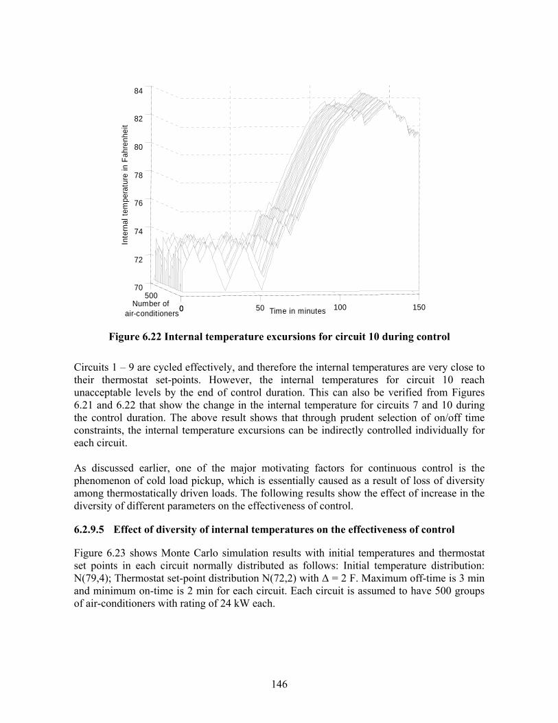
146
0 50 100 1500500
70
72
74
76
78
80
82
84
Time in minutesNumber of
air-conditioners
Inte
rnal
tem
pera
ture
in F
ahre
nhei
t
Figure 6.22 Internal temperature excursions for circuit 10 during control
Circuits 1 – 9 are cycled effectively, and therefore the internal temperatures are very close to their thermostat set-points. However, the internal temperatures for circuit 10 reach unacceptable levels by the end of control duration. This can also be verified from Figures 6.21 and 6.22 that show the change in the internal temperature for circuits 7 and 10 during the control duration. The above result shows that through prudent selection of on/off time constraints, the internal temperature excursions can be indirectly controlled individually for each circuit.
As discussed earlier, one of the major motivating factors for continuous control is the phenomenon of cold load pickup, which is essentially caused as a result of loss of diversity among thermostatically driven loads. The following results show the effect of increase in the diversity of different parameters on the effectiveness of control.
6.2.9.5 Effect of diversity of internal temperatures on the effectiveness of control
Figure 6.23 shows Monte Carlo simulation results with initial temperatures and thermostat set points in each circuit normally distributed as follows: Initial temperature distribution: N(79,4); Thermostat set-point distribution N(72,2) with Δ = 2 F. Maximum off-time is 3 min and minimum on-time is 2 min for each circuit. Each circuit is assumed to have 500 groups of air-conditioners with rating of 24 kW each.

147
As can be seen, with the above initial temperature and thermostat set-point distributions, the chosen on/off time constraints are too stringent. The standard deviation of initial temperature distribution is increased to N(79,20) while maintaining the same distribution for the thermostat set-points. With the maximum off-time and minimum on-time same as above, Monte Carlo simulation results are shown in Figure 6.24. It can be inferred that an increase in the diversity of the initial temperature distribution does not have a significant effect on the effectiveness of control as performance based load levels are still not satisfied over the time interval. This could be attributed to the initial scenario used for the optimization algorithm. Although the initial temperatures are more distributed, the diversity does not affect the control scenario
0
50
100
150
02
46
810
-10
-5
0
5
10
15
Time in minutesNumber of runs
Per
form
ance
bou
ndar
y vi
olat
ion
in M
W
Figure 6.23 Representative Monte Carlo simulation results
with initial temperature distribution N(79,4)
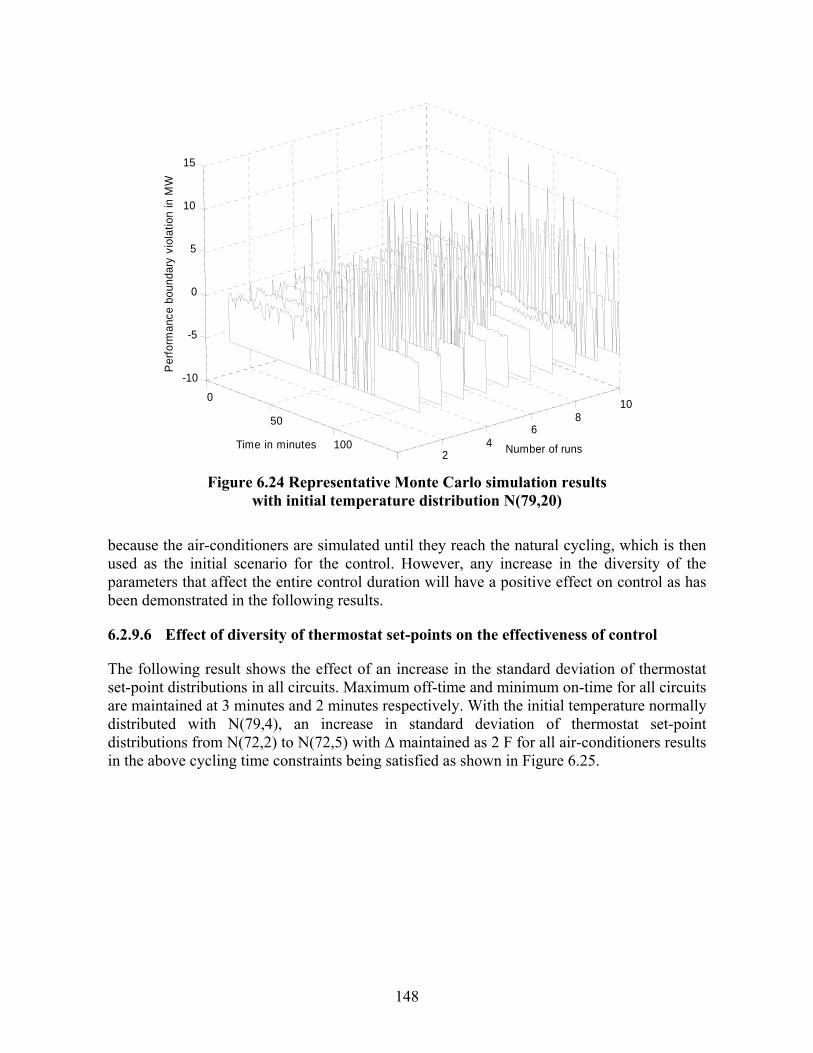
148
0
50
100
15002
46
810
-10
-5
0
5
10
15
Number of runsTime in minutes
Per
form
ance
bou
ndar
y vi
olat
ion
in M
W
Figure 6.24 Representative Monte Carlo simulation results
with initial temperature distribution N(79,20) because the air-conditioners are simulated until they reach the natural cycling, which is then used as the initial scenario for the control. However, any increase in the diversity of the parameters that affect the entire control duration will have a positive effect on control as has been demonstrated in the following results.
6.2.9.6 Effect of diversity of thermostat set-points on the effectiveness of control
The following result shows the effect of an increase in the standard deviation of thermostat set-point distributions in all circuits. Maximum off-time and minimum on-time for all circuits are maintained at 3 minutes and 2 minutes respectively. With the initial temperature normally distributed with N(79,4), an increase in standard deviation of thermostat set-point distributions from N(72,2) to N(72,5) with Δ maintained as 2 F for all air-conditioners results in the above cycling time constraints being satisfied as shown in Figure 6.25.
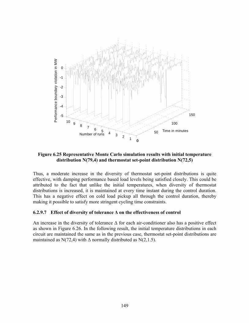
149
0
50
100
150
012345678910-5
-4
-3
-2
-1
0
Time in minutesNumber of runs
Per
form
ance
bou
ndar
y vi
olat
ion
in M
W
Figure 6.25 Representative Monte Carlo simulation results with initial temperature
distribution N(79,4) and thermostat set-point distribution N(72,5) Thus, a moderate increase in the diversity of thermostat set-point distributions is quite effective, with damping performance based load levels being satisfied closely. This could be attributed to the fact that unlike the initial temperatures, when diversity of thermostat distributions is increased, it is maintained at every time instant during the control duration. This has a negative effect on cold load pickup all through the control duration, thereby making it possible to satisfy more stringent cycling time constraints.
6.2.9.7 Effect of diversity of tolerance Δ on the effectiveness of control
An increase in the diversity of tolerance Δ for each air-conditioner also has a positive effect as shown in Figure 6.26. In the following result, the initial temperature distributions in each circuit are maintained the same as in the previous case, thermostat set-point distributions are maintained as N(72,4) with Δ normally distributed as N(2,1.5).

150
0 50 100 15005
10
-4.5
-4
-3.5
-3
-2.5
-2
-1.5
-1
-0.5
0
0.5
Time in minutesNumber of runs
Per
form
ance
bou
ndar
y vi
olat
ion
in M
W
Figure 6.26 Representative Monte Carlo simulation results with diversity in Δ
Similar to thermostat set-points, an increase in the diversity of tolerance Δ also is maintained at each time instant during the control duration, thereby reducing the effect of cold load pickup.
6.2.10 Monte Carlo Simulation Results with Constraints on Temperature Excursions
Following results demonstrate the effect of constraints on the internal temperature excursions. Following are the data corresponding to operating conditions assumed: Number of feeders = 10 (corresponding to D51_1 – D51_5 and D61_1 – D61_5 in Figure 5.5 of the augmented Nordic system) Number of groups of air-conditioners in each feeder = 100 Rating of each group = 120 KW Total maximum controllable load in each feeder = 12 MW Uncontrollable load in each feeder = 13.6 MW Initial internal temperatures: Normal distribution N(79,10) Air-conditioner model parameters: τ – N(64, 10), Tg = N(30,5) Thermostat set-point: N(72,4); Δ = 1.5 F Ambient temperature variation: 1 to 100 min – 89 F; 101 to 150 min – 95 F 151 to 200 min – 90 F; 201 to 250 min – 85 F
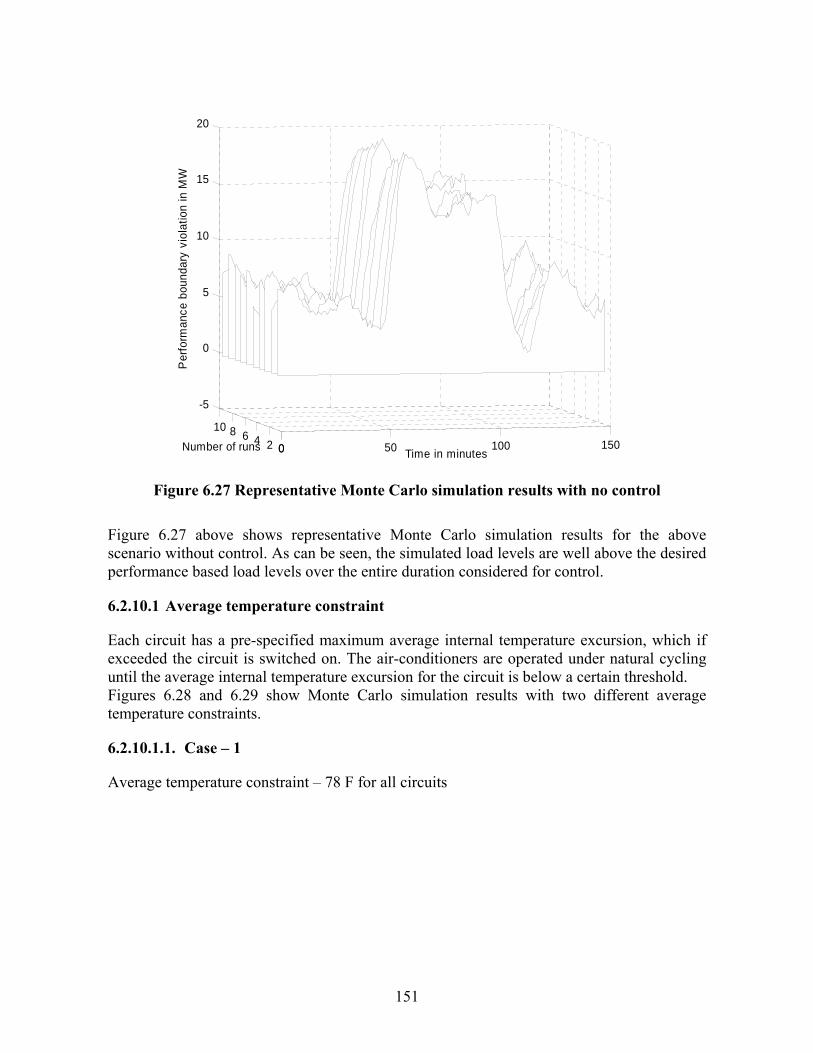
151
0 50 100 1500246810
-5
0
5
10
15
20
Time in minutesNumber of runs
Per
form
ance
bou
ndar
y vi
olat
ion
in M
W
Figure 6.27 Representative Monte Carlo simulation results with no control
Figure 6.27 above shows representative Monte Carlo simulation results for the above scenario without control. As can be seen, the simulated load levels are well above the desired performance based load levels over the entire duration considered for control.
6.2.10.1 Average temperature constraint
Each circuit has a pre-specified maximum average internal temperature excursion, which if exceeded the circuit is switched on. The air-conditioners are operated under natural cycling until the average internal temperature excursion for the circuit is below a certain threshold. Figures 6.28 and 6.29 show Monte Carlo simulation results with two different average temperature constraints.
6.2.10.1.1. Case – 1
Average temperature constraint – 78 F for all circuits

152
050
100
150
02
46
810
-4
-3
-2
-1
0
Time in minutesNumber of runs
Per
form
ance
bou
ndar
y vi
olat
ion
in M
W
Figure 6.28 Representative Monte Carlo simulation results
with avg. temperature constraint – 78 F for all circuits Through repeated simulations by varying the average temperature constraint at different time instants, the lowest average temperature that results in satisfying the desired performance based load levels has been found to be 78 F at all time instants.
6.2.10.1.2. Case – 2
Average temperature constraints 1 min to 50 min – 75 F for all circuits 51 min to 100 min – 78 F for all circuits 100 min to 150 min – 77 F for all circuits
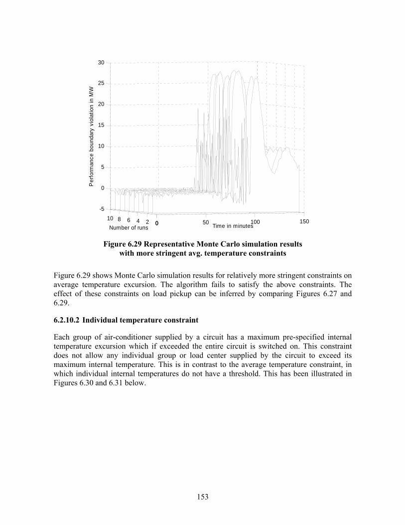
153
0 50 100 1500246810-5
0
5
10
15
20
25
30
Time in minutesNumber of runs
Per
form
ance
bou
ndar
y vi
olat
ion
in M
W
Figure 6.29 Representative Monte Carlo simulation results
with more stringent avg. temperature constraints Figure 6.29 shows Monte Carlo simulation results for relatively more stringent constraints on average temperature excursion. The algorithm fails to satisfy the above constraints. The effect of these constraints on load pickup can be inferred by comparing Figures 6.27 and 6.29.
6.2.10.2 Individual temperature constraint
Each group of air-conditioner supplied by a circuit has a maximum pre-specified internal temperature excursion which if exceeded the entire circuit is switched on. This constraint does not allow any individual group or load center supplied by the circuit to exceed its maximum internal temperature. This is in contrast to the average temperature constraint, in which individual internal temperatures do not have a threshold. This has been illustrated in Figures 6.30 and 6.31 below.

154
0 50 100 150020406080100
60
65
70
75
80
85
90
Time in minutesNumber of air-conditioners
Inte
rnal
tem
pera
ture
in F
ahre
nhei
t
Figure 6.30 Internal temperature excursions during control for circuit 4,
with average temperature constraint Through repeated Monte Carlo simulations by varying individual maximum internal temperature constraint, it has been found that the lowest maximum internal temperature constraint corresponds to 82 F for all circuits. Figure 6.30 shows the change in internal temperatures during the control duration for circuit 4 with average internal temperature constraint of 78 F for the entire duration. Figure 6.31 shows the change in internal temperatures with individual maximum internal temperature constraint of 82 F. As can be seen from Figure 6.30, individual internal temperatures reach levels well above the chosen threshold for the entire circuit. However, with individual constraints, the worst-case internal temperature excursions are bounded.

155
0 50 100 150020406080100
64
66
68
70
72
74
76
78
80
82
84
Time in minutesNumber of
air-conditioners
Inte
rnal
tem
pera
ture
in F
ahre
nhei
t
Figure 6.31 Internal temperature excursions during control for circuit 4,
with individual maximum temperature constraint
6.2.10.3 Effect of increase in uncontrollable load on internal temperature excursions
The above DP algorithm with internal temperature excursion constraints provides a framework to study the effect of increase in uncontrollable load on internal temperature excursions. With the maximum individual internal temperature excursion assumed the same for all circuits, the following result in Figure 6.32 shows the optimum increase in internal temperature excursions with uncontrollable load levels in different circuits. For the same performance based boundary, as uncontrollable load levels are increased, the maximum internal temperature excursion constraints need to be relaxed in order to be able to satisfy the boundary load levels. The maximum internal temperature excursion shown in the figure is percentage of the mean of thermostat distribution assumed for each circuit. As the uncontrollable load increases, the optimum percentage increase in thermostat set-point for each group also increases proportionally.

156
112 114 116 118 120 122 124 126 128 13011
11.5
12
12.5
13
13.5
14
14.5
Percentage of mean of thermostat set-point distribution
Unc
ontro
llabl
e lo
ad in
the
circ
uit i
n M
W
Figure 6.32 Optimum increase of internal temperatures with increase
in uncontrollable load levels
6.2.10.4 Equivalence between cycling time constraints and temperature excursion constraints
The following result shows the equivalence between on/off time constraints and average internal temperature constraint for the operating conditions assumed earlier in the beginning of this section. Average temperature constraint for all circuits of 78 F is satisfied as shown by a representative result of load levels after control in Figure 6.33. With the above constraint, Figures 6.34 – 6.36 show the distribution of internal temperatures at three different time instants during the control duration, at 50 min, 100 min and 150 min respectively for a representative circuit.

157
0 50 100 150-6
-5
-4
-3
-2
-1
0
Time in minutes
Per
form
ance
bou
ndar
y vi
olat
ion
in M
W
Figure 6.33 Representative load levels after control with avg. temperature constraint
65 70 75 80 850
5
10
15
20
25
Internal temperature in Fahrenheit
Num
ber o
f air-
cond
ition
ers
Figure 6.34 Internal temperature distribution at t=50 min
(Avg. temperature constraint)
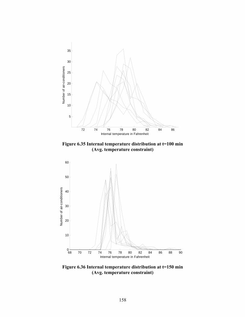
158
72 74 76 78 80 82 84 86
5
10
15
20
25
30
35
Internal temperature in Fahrenheit
Num
ber o
f air-
cond
ition
ers
Figure 6.35 Internal temperature distribution at t=100 min
(Avg. temperature constraint)
68 70 72 74 76 78 80 82 84 86 88 900
10
20
30
40
50
60
Internal temperature in Fahrenheit
Num
ber o
f air-
cond
ition
ers
Figure 6.36 Internal temperature distribution at t=150 min
(Avg. temperature constraint)

159
With maximum off-time of 3 min and minimum on-time of 2 min, Figure 6.37 shows a representative result of load levels that satisfy the desired performance boundary closely.
0 50 100 150-6
-5
-4
-3
-2
-1
0
Time in minutes
Per
form
ance
bou
ndar
y vi
olat
ion
in M
W
Figure 6.37 Representative load levels after control with on/off time constraints
With the above operating conditions and cycling time constraints, Figures 6.38 – 6.40 show the distribution of internal temperatures at 50 min, 100 min and 150 min during the control duration.

160
65 70 75 80 85 90
5
10
15
20
25
Internal temperature in Fahrenheit
Num
ber o
f air-
cond
ition
ers
Figure 6.38 Internal temperature distribution at t=50 min (on/off time constraints)
72 74 76 78 80 82 84 860
5
10
15
20
25
30
35
40
Internal temperature in Fahrenheit
Num
ber f
o ai
r-con
ditio
ners
Figure 6.39 Internal temperature distribution at t=100 min (on/off time constraints)
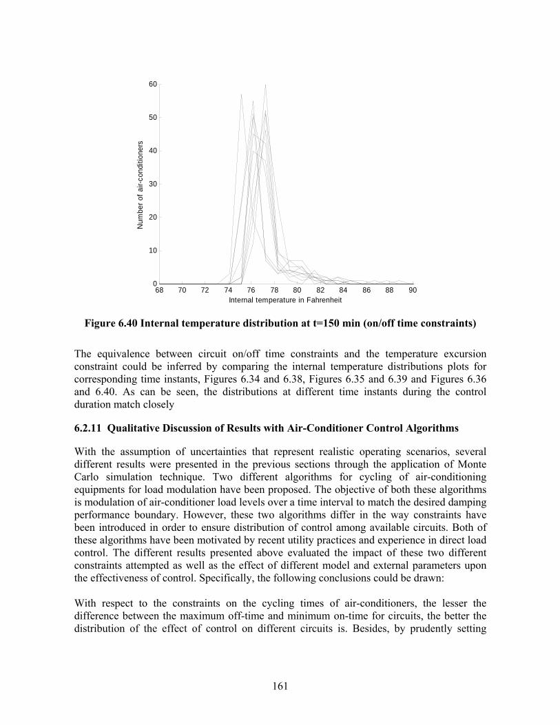
161
68 70 72 74 76 78 80 82 84 86 88 900
10
20
30
40
50
60
Internal temperature in Fahrenheit
Num
ber o
f air-
cond
ition
ers
Figure 6.40 Internal temperature distribution at t=150 min (on/off time constraints)
The equivalence between circuit on/off time constraints and the temperature excursion constraint could be inferred by comparing the internal temperature distributions plots for corresponding time instants, Figures 6.34 and 6.38, Figures 6.35 and 6.39 and Figures 6.36 and 6.40. As can be seen, the distributions at different time instants during the control duration match closely
6.2.11 Qualitative Discussion of Results with Air-Conditioner Control Algorithms
With the assumption of uncertainties that represent realistic operating scenarios, several different results were presented in the previous sections through the application of Monte Carlo simulation technique. Two different algorithms for cycling of air-conditioning equipments for load modulation have been proposed. The objective of both these algorithms is modulation of air-conditioner load levels over a time interval to match the desired damping performance boundary. However, these two algorithms differ in the way constraints have been introduced in order to ensure distribution of control among available circuits. Both of these algorithms have been motivated by recent utility practices and experience in direct load control. The different results presented above evaluated the impact of these two different constraints attempted as well as the effect of different model and external parameters upon the effectiveness of control. Specifically, the following conclusions could be drawn: With respect to the constraints on the cycling times of air-conditioners, the lesser the difference between the maximum off-time and minimum on-time for circuits, the better the distribution of the effect of control on different circuits is. Besides, by prudently setting

162
cycling times for circuits, the distribution of control among different circuits could be controlled. The effect of an increase in the diversity of thermostat set-points results in minimizing the effect of cold load pickup thereby satisfying more stringent cycling time constraints. However, an increase in diversity of initial temperature distributions fails to have a positive effect on control. This is on account of the fact that the initial scenario considered for control corresponds to natural cycling of air-conditioners and hence the diversity of initial temperatures is not perceivable during the control duration. On the other hand, an increase in the diversity of air-conditioner model parameters has a lasting effect throughout the control duration and hence has a positive effect on the effectiveness of control. With regard to internal temperature excursions constraints, two different constraints are possible, namely, an average temperature excursion constraint for the feeder and a maximum temperature excursion constraint for each group in a feeder. Both of these constraints have been demonstrated along with their distinguishing effects. The modeling of temperature excursion constraints in the DP algorithm provides an optimization framework to study the effect of an increase in load levels on the discomfort caused as a result of internal temperature excursions. This has been demonstrated with the small-signal stability performance boundary obtained for the augmented Nordic system. Finally, the equivalence between the cycling time constraints and the temperature excursion constraints has also been demonstrated. Thus, although these two constraints are conceptually different in their implementation, both attempt effective cycling of air-conditioners and their equivalence has been established.
6.3 Water-Heater Control – Optimization Framework
6.3.1 Model of a Domestic Water-Heater
The concepts behind the model proposed in [103] for a domestic water-heater form the foundation of the algorithm proposed for water-heater control. Following is an overview of the water-heater model. The development of the model is based on the usage characteristics of domestic water-heaters represented in a histogram as shown in Figure 6.41. The histogram shows the number of hot water usage events by a certain population of customers during a time interval.

163
Figure 6.41 Example histogram of usage of domestic water-heaters
The following assumptions are made with respect to the above histogram in the development of a model for the water-heater.
i) Every usage event is recorded for a different water-heater ii) A fixed amount of water is drawn every time
The above two assumptions make it possible to calculate how long a representative water-heater would remain on before the water that refilled the storage vessel is heated. The amount of energy that must be added to the storage vessel is
Q= m.C. ΔT Joules (6.4)
where m is the mass of water in kg (or volume of water in liters since 1 liter of water weighs 1 kg), C is the specific heat of water and ΔT is the required temperature rise of the added water in 0C. The time for which the water heater element must be maintained on to add this amount of energy is
ton = Q/(60 Pe) min (6.5)
where Pe is the power rating of the water heater element in kW. Let Pe = 3 kW, ΔT = 40 0C, m = 65 kg, C = 4200 J/kg/0C
Then, ton = 60 min. Thus every storage water-heater from which water is drawn during a certain 20 minutes’ interval in Figure 6.41 will remain on for that time interval and following two consecutive 20 minute intervals. Thus, corresponding to the usage pattern shown in Figure 6.41, Figure 6.42 shows the cumulative number of water-heater usage at each time interval. The units of the y-axis can be easily converted to kW simply by multiplying with the average rating of water heaters.
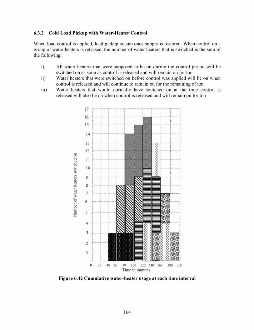
164
6.3.2 Cold Load Pickup with Water-Heater Control
When load control is applied, load pickup occurs once supply is restored. When control on a group of water heaters is released, the number of water heaters that is switched is the sum of the following:
i) All water heaters that were supposed to be on during the control period will be switched on as soon as control is released and will remain on for ton
ii) Water heaters that were switched on before control was applied will be on when control is released and will continue to remain on for the remaining of ton
iii) Water heaters that would normally have switched on at the time control is released will also be on when control is released and will remain on for ton
Figure 6.42 Cumulative water-heater usage at each time interval

165
6.3.3 Decision Tree-Based Water-Heater Control Algorithm
6.3.3.1 Data requirements for executing real-time control of water-heaters
In order to model and thereby predict and control cold load pickup when executing control, it is essential to determine the number of water-heaters in the group that are switched on at discrete intervals of time, say of 20 or 30 minutes’ duration. Following are two different approaches towards the determination of the above.
6.3.3.1.1. Approach I
With the average value of the active power load profile during an interval known, reference [103] presents a methodology to calculate the number of water-heaters that are switched on during the interval. The average value of the active power load could be obtained through a very short-term load forecast. Let a day be divided into M time intervals (For 20 minutes’ time intervals, M=24x60/20= 72). Let Pi be the average value of the load profile for the ith time interval in watts. The amount of energy equivalent is
Qi = Pi. τ. 60 Joules (6.6)
where τ is the time interval in minutes. Let Qtot be the amount of energy represented by the entire load profile for the day.
Qtot = ∑M
iQ1
Joules (6.7)
The average amount of energy Qavg consumed by each usage event is then obtained from (6.4) as follows:
Qavg= m.C. ΔTavg Joules (6.8)
Average inlet temperature and thermostat settings are used to calculate ΔTavg. Having obtained Qavg, the average number of usage events per day is calculated next as
avgtot
totavg
QNQF = (6.9)
pi = Qi/Qtot is the normalized probability of a water heater being switched on at during the ith
time interval ( 11
=∑M
ip ). Every usage event will result in the water-heater remaining in the
on state for N intervals (=ton minutes). Then the portion of water-heaters that are on during the ith interval is
Qi = pi + pi-1 + pi-2 + ….. + pi-(N-1) (6.10)
The number of water-heaters that will be on during the ith time interval is
Non i = Ntot Qi Favg (6.11)

166
6.3.3.1.2. Approach II
Alternatively, reference [100] assumes a Gaussian probability distribution for the number of households n that use hot water at time t
n(t) = Ntot
20
21
21 ⎟
⎠⎞
⎜⎝⎛ −
−σ
πσ
tt
e (6.12)
where Ntot is the total population, σ is the measure of the width of the distribution in minutes, and t0 is the time at which most people use hot water. The number of hot water cylinders which have been switched on by time t1 is the area under the probability curve up to time t1.
⎟⎠⎞
⎜⎝⎛ −
Δ=⎟⎠⎞
⎜⎝⎛ −
−
∞− ∞−∫ ∫ σπσσ 012
1 20
1 1
21)( tterfNdteNtn tot
ttt t
tot (6.13)
The number of water heaters turned on at time t1, N(t1), is the sum of all water heaters turned on between t1 – ton and t1. This is because the heaters switched on before t1 – ton would have already switched off at time t1. Therefore,
N(t1) = ⎥⎦
⎤⎢⎣
⎡⎟⎠⎞
⎜⎝⎛ −−
−⎟⎠⎞
⎜⎝⎛ −
σσon
totttterftterfN 0101 (6.14)
The total power consumed by the cylinders that are on is
Ptot(t1)=Pe N(t1) (6.15)
Power per hot water cylinder is: P(t1) = Ptot(t1)/Ntot
= ⎥⎦
⎤⎢⎣
⎡⎟⎠⎞
⎜⎝⎛ −−
−⎟⎠⎞
⎜⎝⎛ −
σσon
ettterftterfP 0101 (6.16)
6.3.3.2 Control algorithm
Basic setup
• The entire time period during which significant usage of water heaters is observed (it could be morning or evening depending on the lifestyle, climatic and several other conditions) is divided into several intervals, say of 20 minutes’ duration.
• There are several groups or circuits of water heaters supplied, say one by each distribution feeder. Each group of water heaters has its own usage pattern.
• Control is executed on the group as a whole.

167
• At each time interval, electrical load is the sum of the following: uncontrollable load and controllable water heater load.
• The number of water heaters that are on during any time interval t is the sum of water heaters that are switched on during interval t and those that are switched on between intervals t-ton+1 and t-1 (on account of on-time for water heaters).
At the highest level, the algorithm consists of checking one time interval ahead from the current interval as to whether the performance boundary would be violated as a result of water heater load during that interval. There are two possible actions based on the outcome:
1. If the performance boundary would be violated, water heaters that would be newly switched on at that interval are not allowed to switch on. If violation of the boundary persists, water heaters that have been previously switched on and those that contribute to the load during the time interval under consideration (on account of their on-time) are switched off starting with the current interval and proceeding in descending order of time intervals. This is repeated until the load level one interval ahead is such that the point of operation is within the performance boundary.
2. If there is no performance boundary violation for the time interval ahead, it is
attempted to increase the load level by switching on water heaters that were previously switched off as a result of control. Switching on is performed in ascending order of time. For a particular time, the order in which the water heaters are switched on is the reverse of the order in which they were switched off. This ensures continuity of supply for a group when switched on. This step is repeated until the loading is at a level such that further increase by switching on previously off water heaters would cause the performance boundary to be violated.
The algorithm is based on a decision-tree search approach as shown in Figure 6.43 below. The steps are as follows: Step 1: At time t, calculate total load at time t+1 and check for violation of small-signal performance boundary. If there is no violation, proceed to step 4.
Step 2(i): Arrange the circuits in ascending order of the total number of water heaters that would be switched on at time t+1.
Step 2(ii): Calculate load and small-signal performance boundary by shutting down water heaters that are supposed to be switched on at t+1 in the order established in Step 2(i). Repeat this step until either the load at time t+1 has reduced to a level such that the small-signal performance boundary is not violated or all water heaters supposed to be switched on have been switched off. If boundary violation persists after this step go to step 2(iii). Else go to step 2(iv)
Step 2(iii): The load at t+1 is also due to water heaters that are switched on between t-ton+1 and t-1. This is because each water heater switched at any time remains on for duration equal to its on-period. Starting at t-1 time interval and proceeding to t-ton+1 by decrementing by

168
one interval, arrange circuits of water heaters in ascending order of the number of water heaters that are on at each time interval.
Step 2(iv): Calculate load and small-signal performance boundary by shutting down water heaters that are already on (and contribute to load at t+1) in the order established in step 2(iii).
Step 2(v): Repeat steps 2(iii) and 2(iv) until load at time t+1 has reduced to a level such that the small-signal performance boundary is not violated. Go to Step 7.
Step 3: Go to step 4 if water heaters were previously switched off at any time prior to t+1 on account of control. Else go to step 7.
Step 4: Start at the first time interval during which control is executed.
Step 5: Switch on water heaters at t+1 in the reverse order in which they were switched off for that interval under consideration (Reverse order ensures continuity of supply to a group of water heaters once switched on).
Step 6: Repeat step 5 by incrementing by one interval until one of the following outcomes is reached: Either load at t+1 is such that further increase would result in violation of performance boundary or all previously switched off water heaters have been switched on.
Step 7: Increment t and go to step 1.

169
Figure 6.43 Decision-tree based search algorithm for water-heater control
Check performance boundary violation
at t+1
Switch off groups of water heaters that would be switched
on at t+1
All groups tried?
Check perf. boundary
violation at t+1
Switch off groups of water heaters previously
switched on and that contribute to load at t+1
Check perf. boundary
violation at t+1
All groups tried?
All previous time intervals
tried? Decrement time
Check if any group was previously off due to control in ascending
order of time
Switch on groups
previously off for that time
Check performance boundary violation
at t+1
All groups switched on?
All previous time intervals taken care of?
Increment time
At time t
Yes
No
Violated
No violation
No violation
Violated
Yes
No
No
No violation Violated
Stop
NoYes
Vio
late
d
Yes
No
No
Stop
Yes
No violation
t t+1

170
6.3.3.3 Numerical result and simulation
Number of feeders = 10 (corresponding to D51_1 – D51_5 and D61_1 – D61_5 in Figure 5.5 of the augmented Nordic system)
Rating of each water-heater = 4 kW
Total maximum controllable load from water-heaters in each feeder = 12 MW
Uncontrollable load in each feeder = 11 MW
Identical usage patterns have been assumed for all feeders. This corresponds to the worst-case because the peak loads occur at the same time.
Table 6.1 shows the usage pattern and the corresponding controllable load levels similar to the data available in [103].
Table 6.1 Usage pattern and water-heater load levels
Time interval (in minutes)
Water-heater usage (in Numbers)
Cumulative usage with ton(= 60 mins)
Water heater load in MW
0 – 20 0 0 0 20 – 40 0 0 0 40 – 60 400 400 1.6 60 – 80 600 1000 4 80 – 100 750 1750 7 100 – 120 900 2250 9 120 – 140 1000 2650 10.6 140 – 160 850 2750 11.0 160 – 180 800 2650 10.6 180 – 200 600 2250 9 200 – 220 480 1880 7.52 220 – 240 200 1280 5.12 240 – 260 0 680 2.72 260 – 280 0 200 0.8 280 – 300 0 200 0.8
Corresponding to the above controllable and uncontrollable load levels, the performance boundary violation is shown in Table 6.2. Control is initiated at t = 100 min and is executed until t = 280 min. Figure 6.44 shows the performance boundary violation with and without control.

171
Table 6.2 Performance boundary violation with simulated load levels, with and without control
Time interval (in minutes)
Performance boundary
violation in MW before control
Performance boundary
violation in MW with control
0 – 20 -40.8 -40.8 20 – 40 -40.8 -40.8 40 – 60 -32.56 -32.56 60 – 80 -20.2 -20.2 80 – 100 -4.75 -4.75 100 – 120 5.55 -1.79 120 – 140 13.79 -0.57 140 – 160 15.85 -1.66 160 – 180 13.79 -1.03 180 – 200 5.55 -0.57 200 – 220 -2.07 -0.24 220 – 240 -14.43 -3.01 240 – 260 -26.79 -1.72 260 – 280 -36.68 -0.24 280 – 300 -40.8 -37.13
0 50 100 150 200 250 300-50
-40
-30
-20
-10
0
10
20
Time in minutes
Per
form
ance
bou
ndar
y vi
olat
ion
in M
W
No controlAfter control
Figure 6.44 Performance boundary violation with and without control
Control initiated
Control executed during these
intervals
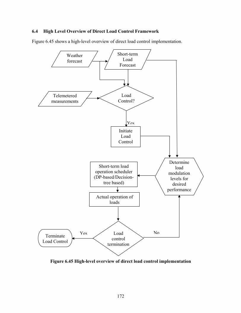
172
6.4 High Level Overview of Direct Load Control Framework
Figure 6.45 shows a high-level overview of direct load control implementation.
Figure 6.45 High-level overview of direct load control implementation
Telemetered measurements
Weather forecast
Short-term Load
Forecast
Load Control?
YesInitiate Load
Control
Determine load
modulation levels for desired
performance
Short-term load operation scheduler
(DP-based/Decision-tree based)
Actual operation of loads
Load control
termination
NoTerminate
Load Control
Yes

173
7. Conclusions and Future Work
7.1 Conclusions
In this research, the application of direct load control to enhance oscillatory stability in power systems has been investigated. This research has been motivated mainly by the following aspects: need for robust measures for stability performance enhancement, recent increased interest in treatment of loads as system resource, the developments that have taken place in some of the enabling technologies for direct load control and the changing utility business model under deregulation that facilitates participation of loads in supplying some of the reliability services. Within the broader objective of reliability enhancement through direct load control, this research has focused on enhancing small-signal stability performance through direct non-disruptive control of selected active power loads. Two main contributions of this research are the following: 1) Development of an analysis framework and 2) conceptually different analysis approaches for load modulation to enhance oscillatory stability and the development and study of algorithms for real-time modulation of certain selected loads based on the results from the analysis. The specific contributions of this research can be summarized as follows:
1. Development of a linear model for the problem of direct load control – This linear model is the basis for the analysis framework. This linear model has been applied in selecting the optimal locations for load modulation through a comprehensive modal analysis. The important differentiating characteristic of the linear model for direct load control from those used in other power system control designs is based on the principle that the load available for control at a bus is modeled as an input to the system. This allows the use of different load models for controllable load at each load bus and is essential to characterize the uncertainty in the controllable part of the load. Besides, this is also important for modal analysis, especially in calculating Eigen-value sensitivity for active power loads, and in the determination of controllability of selected modes from load inputs.
2. Development of an analysis framework for load modulation through the application
of robust performance theorem, one of the fundamental theorems related to Structured Singular Value concept. The above framework for analysis has been developed by casting the linear model developed for direct load control into a form suitable for the application of robust performance theorem. The uncertainty in the operating conditions in terms of load levels or generation is real-parametric uncertainty and could be represented in a structured form thereby making it possible for SSV-based analysis. A framework for robust performance analysis is developed from a Linear Fractional Transformation (LFT) representation of uncertainty in the state-space model and the damping performance specifications in terms of the MIMO H∞ norm.
A simulation-based approach using SIMGUI within Matlab’s MU tools has been developed for the purpose of selecting damping performance specifications.

174
3. Development of analysis approaches for load modulation – Two fundamentally different approaches to analysis of the amount of load modulation for desired stability performance have been developed.
a. Approach I: Determination of worst-case uncertainty for a given performance
specification – In this formulation of the problem, active power load at each load bus selected for control is assumed to be the sum of controllable and uncontrollable parts. Uncertainty is assumed to exist in the controllable part of the loads. The analysis then proceeds to determine the maximum uncertainty range for the controllable as well as the total load levels that satisfies the damping performance specifications. Essentially, in this approach, the uncertainty in load levels is the control variable that is varied until the performance criterion is satisfied.
Analytical proof of the concept – It has been analytically shown that with the above uncertainty characterization and the criterion for performance specification satisfied, it is always possible to determine the maximum uncertainty range in load levels that would satisfy the chosen performance conditions.
b. Approach II: Determination of worst-case performance for a given uncertainty range – This is a fairly general formulation of the problem and it allows uncertainty to exist not only in load levels, but in generation levels as well as in any parameter of the system. Eigenvalue sensitivities have been used in the selection of load buses for control implementation based on the eigenvalue sensitivity of active power loads. Essentially, in this approach, the nominal load levels at certain load buses are the control variables and they are varied until the worst-case performance for the fixed uncertainty range is satisfied.
c. Both the above formulations are skewed – μ formulations in the context of
SSV theory. The first approach is applied with variable load uncertainty bounds and the second approach is applied with uncertainty in load, generation or in any other system parameter, however with fixed bounds.
4. Both the approaches have been tested on two different fairly large and complex
systems: CIGRE Nordic test system and the Western Electric Coordinating Council (WECC) test system. The robustness of the analysis approach, as well as the correctness of the performance characterization and the overall analysis framework have been demonstrated with multiple results on these two different systems. In the determination of load levels that satisfy the chosen damping performance conditions, the analysis could be done at the transmission level of the system. The amount of load to be modulated at the transmission level could then be divided amongst multiple feeders that connect at the transmission level load bus. Alternatively, the system at transmission voltage level could be augmented with sub-

175
transmission and distribution systems and the determination of the amount of load to be modulated could be done at the distribution level. Both these approaches have been illustrated. The CIGRE Nordic system has been augmented with sub-transmission/distribution feeders at selected load buses. A desired stability performance boundary has then been obtained through repeated application of robust performance analysis using approach I. On the other hand, analysis is performed at transmission level on the WECC system.
5. Development and a detailed study of algorithms for real-time modulation of controllable thermal loads – air conditioners and water heaters – based on the results of the analysis described above. Air-conditioners and water-heaters are the loads that have traditionally been controlled in load management programs. In controlling groups of thermostatically driven loads, the phenomenon of cold load pickup needs to be modeled and taken care of. The primary objective is to operate loads as close as possible to the desired load levels obtained from analysis through either of the two approaches. Recent developments in two-way communication as well as in load control systems enable direct load control with minimum discomfort. However, the necessary algorithms and study of the impact of different parameters and variables are lacking. In this research, an attempt has been made to develop and study algorithms for load control with minimum disruption. Thus, besides the objective of minimizing the amount of load controlled, the objective of performing effective cycling of controllable loads is also taken into account. The above problem has been formulated as an optimization problem. Different artificial constraints have been modeled in the optimization problem in order to take care of effective cycling of loads.
6. Two different algorithms based on Dynamic Programming with different sets of
constraints have been proposed for air-conditioner loads, while a decision-tree based search algorithm has been proposed for water-heater loads. The development of these algorithms is in line with some of the most recent load management programs executed. The different constraints that have been attempted are cycling (on/off) time constraints and temperature excursion constraints.
7. An optimization framework has thus been developed employing the above
algorithms. Using this framework, numerous Monte Carlo simulations have been performed with uncertainties modeled in different parameters corresponding to the models as well as external variables that appear in the models. The objective of these simulations is to study in detail the effect of different constraints as well as parameters on the effectiveness of control. A variety of results have been obtained with realistic assumptions of operating conditions and model parameters. Several important conclusions have been drawn from these results concerning control of thermostatically driven loads with minimum disruption.
Broadly, this research has focused on issues involved in utilizing direct load control for
176
dynamic security enhancement. The work presented in this research has studied the type of loads to be controlled, issues involved in controlling selected loads in real-time and algorithms for performing real-time load modulation. The necessary framework and approaches for analyzing the amount of load modulation have also been developed through the application of Structured Singular Value theory. The primary results of this research clearly demonstrate a great potential for the application of direct load control for small-signal stability performance enhancement. The efficacy as well as the robustness of the scheme has been demonstrated over a range of operating conditions on different test systems. Incorporating direct load control through modulation of a fraction of the total load in the system can significantly enhance system security. Through proper selection of type of loads as well as their locations for control implementation, and through optimizing the duration of control action, it is possible to execute control with minimum disruption/discomfort. Modern sensor and communication technology facilitates such an approach. The conclusions drawn from this research strongly advocate direct load control for stability enhancement from the perspectives of effectiveness of control, robustness of the scheme, economic viability of the technology, and fast availability of the institutional framework for the participation of loads in providing system reliability services.
7.2 Future Work
The diverse nature of the topic as well as the nascency of the concept of direct load control for reliability enhancement opens up several possibilities for future work in widely different, however very relevant areas. Some of them have been summarized in the following: Techniques to speed-up the analysis of load modulation: Load modulation for stability enhancement is being proposed as an online tool and hence timely execution of analysis is very critical. Although robust control tools and techniques are very powerful for analysis and design of control structures in the presence of uncertainties, the algorithms are computationally highly intensive. However, enhancement of computational techniques in the area of robust control is one of the most active areas of research within modern control systems. These advancements could be usefully exploited. In particular, certain characteristics unique to power system computation could be utilized in significantly reducing computational burden involved in the analysis. One such technique was illustrated in Section 5.3.1 with regard to updating the linear curve-fitting coefficients. Also, for large systems sparsity based computational techniques will offer significant reduction in the computational time. Power system modeling using Prony analysis: The approach adopted in this research for the development of a power system linear model for direct load control is a component based approach. The order of the model depends on the number of dynamic devices, which for large systems could become intractable. Prony analysis based modeling is a promising alternative to component-based model construction and has been successfully applied in several recent researches. It is a signal processing methodology that extends Fourier analysis and makes it possible to estimate the model from transient stability program simulations. The

177
numerical advantages of Prony analysis make it well suited for approximating higher order signals with an optimum low order model. The model order is dependent on desired accuracy. However, uncertainty modeling with such a model obtained through Prony analysis, in which the model parameters do not directly correspond to system components and parameters, will have to be explored. Selection of weighting functions: In this work, weighting functions for performance characterization are selected based on trial and error. It would be very useful to devise certain rules based on which weighting functions could be chosen for specified performance. Based on several offline studies, such rules could be devised for a given system. These rules could then be built into the load modulation analysis algorithm, which could construct weights based on performance specifications. These weights can further be utilized in analysis of the amount of load modulation. Detailed load modeling: The effect of more detailed modeling of loads could be explored. In this work, although the linear model as well as the analysis framework developed allows consideration of dynamic load models, both controllable and uncontrollable loads have been modeled with as static voltage dependent loads. Controllable air-conditioner loads could be accurately modeled as induction motor loads. Uncontrollable load models could also be modeled using aggregate dynamic models in order to study their impact more accurately. Development of competitive framework: Issues related to the integration of a scheme to procure loads for stability enhancement in a deregulated market structure could be studied. One approach for such a microeconomic framework would be to assume utility functions for groups of consumers, with individual utility functions dependent on the amount of discomfort. In a market for interruptible load, customer participation would then depend on the trade-off between economic incentive from the market and the utility that would need to be sacrificed upon interruption. Communication and information architecture requirements for integration into a state-of-the-art Energy Management System (EMS): The type of information/communication architecture required as well as data requirements and data exchange mechanisms needed in order for a direct load control scheme to be integrated into an EMS could be explored. Successful, high-fidelity operation of this scheme would require careful coordination of EMS (at transmission level) and Distribution Management System (DMS – at sub-transmission/distribution level). Such coordination does not exist in practice today. However, with increasing interest in distributed energy resources, the need for such coordination is strongly felt. Multi-agent based computation for direct load control: There has been a recent surge in interest on agent-based computation for power system applications. An agent in the context of computer science is defined as a component of software and/or hardware, which is capable of acting in order to accomplish tasks on behalf of its user. One of the foremost reasons for interest in agent-based computation is the fact that the emerging power system operation is open and dynamic. There could be entities in such an environment that may require

178
computation and communication resources depending on certain outcomes. Direct load control for reliability enhancement could be considered as one such application. This is because the need for load control would depend on system vulnerability and possible contingencies. Agent-based approach to computation and communication allows allocation of resources dynamically in real-time without dedicated allocation and is very attractive for applications such as direct load control. Detailed modeling of stochastic effects and stochastic dynamic programming: The impact of weather uncertainty, short-term load forecast uncertainty and unmodeled weather characteristics on the effectiveness of control strategy could be examined through the application of stochastic dynamic programming framework.

179
Appendix A Sub-transmission/distribution system feeder design details
Figure A.1 One-line diagram of sub-transmission/distribution feeder
Figure A.1 shows the one-line diagram of the feeder to be designed. The typical transformer and line design data available in [142] has been utilized in the design of the feeder.
System parameters
130/46.5 KV transformer
The p.u .reactance of the transformer is 0.08 p.u. on its own base
Assuming a base of 80 MVA for the transformer, its p.u. reactance on 100 MVA base is
0.1000 p.u.
Line 1
Maximum load served is assumed to be 70 MVA
Maximum current carrying capacity = 70 x 1000/ (1.732 x 130) = 311 Amps
Assuming 130 KV line to be made of ACSR Linnet type of conductor,
Resistance = 0.278 Ω/mi.
GMR of ACSR Linnet conductor (from impedance tables) is 0.0244 Ft.
Assuming a distance of separation of 4m (=13.13 ft) between phases,
Inductance = 2 x П x 2 x 10⁻⁷ x ln(6.5633/0.0244) x 1609
= 0.7628 Ω/mi
Assuming a length of 20 mi for line 1,
total Impedance = 5.56+j 15.256 Ω.
Impedance in p.u. for Line 1 = 100 x (5.56+j 15.256)/ (130 x 130)
130/46.5 KV
Line 1 Length=20 mi
13 KV Line 2 Length=8 mi
46.5/13 KV

180
= 0.0329 + j 0.0903 p.u
Adding transformer p.u. reactance, total impedance between 130 KV bus and 46.5 KV bus
= 0.0329 + j(0.0903+0.1) p.u
= 0.0329 + j 0.1903 p.u
46.5/13 KV transformer
The p.u. reactance of the transformer is 0.06 p.u. on its own base.
Assuming a base of 25 MVA for the transformer, its p.u. reactance on 100 MVA base is 0.24 p.u.
Line 2
Maximum load served is assumed to be 25 MVA.
Maximum current carrying capacity = 25 x 1000 / (1.732 x 46.5) = 310 Amps
Assuming 46 KV line to be made of ACSR Ostrich type of conductors,
Resistance = 0.311 Ω/mi
GMR of ACSR Ostrich type of conductor is 0.0241 Ft.
Assuming a distance of separation of 2.5 m (= 8.2017 ft) between phases,
Inductance = 2 x ∏ x 60 x 2 x 10-7 x ln (8.2017/0.0241) x 1609
= 0.7073 Ω/mi
Assuming a length of 8 mi for line 2,
Total impedance = 2.488 + j 5.6584 Ω.
Impedance of line 2 in p.u. = 100 x (2.488 + 5.6584) / (46.5 x 46.5)
= 0.1176 + j0.2674 p.u
Adding transformer p.u. reactance, total impedance between 46.5 KV bus and 13 KV bus
= 0.1176 + j(0.2674+0.24)
= 0.1176 + j 0.5074 p.u.

181
Appendix B Generation and Load Levels for Nordic System for Test Cases Base case generation and load levels for Section 5.3.2.1
Bus Generation in MW Load in MW N4011 800 0 N4012 300 0 N4021 250 0 N4031 650 0 N4042 990 0 N4047 1080 0 N4051 600 0 N4062 850 0 N4063 900 0 N4071 400 600 N4072 900 600 N1012 600 300 N1013 300 400 N1014 550 0 N1021 200 0 N1022 200 380 N2032 530 400 N1042 380 300 N1043 258 150 N1011 0 26 N2031 0 130 N1041 0 370 N1044 0 1040 N1045 0 960 N41 0 500 N42 0 910 N43 0 1200 N46 0 130 N47 0 390 N62 0 420 N63 0 750 N51 0 206 N61 0 206
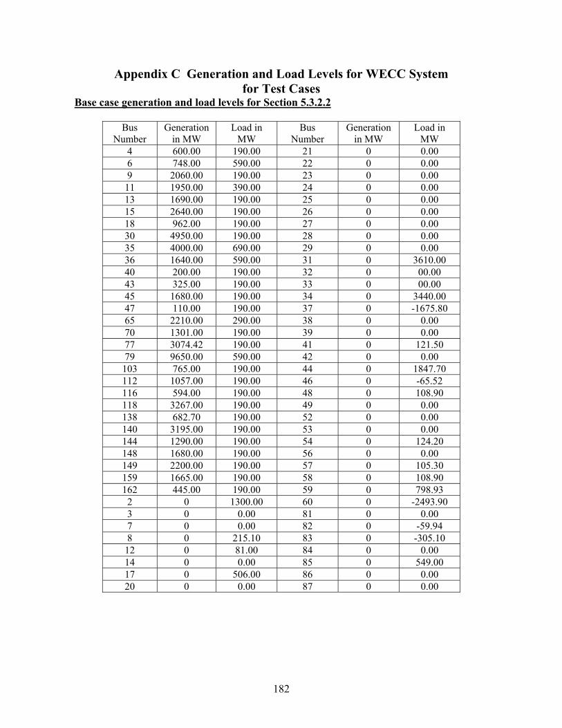
182
Appendix C Generation and Load Levels for WECC System for Test Cases
Base case generation and load levels for Section 5.3.2.2
Bus Number
Generation in MW
Load in MW
Bus Number
Generation in MW
Load in MW
4 600.00 190.00 21 0 0.00 6 748.00 590.00 22 0 0.00 9 2060.00 190.00 23 0 0.00
11 1950.00 390.00 24 0 0.00 13 1690.00 190.00 25 0 0.00 15 2640.00 190.00 26 0 0.00 18 962.00 190.00 27 0 0.00 30 4950.00 190.00 28 0 0.00 35 4000.00 690.00 29 0 0.00 36 1640.00 590.00 31 0 3610.00 40 200.00 190.00 32 0 00.00 43 325.00 190.00 33 0 00.00 45 1680.00 190.00 34 0 3440.00 47 110.00 190.00 37 0 -1675.80 65 2210.00 290.00 38 0 0.00 70 1301.00 190.00 39 0 0.00 77 3074.42 190.00 41 0 121.50 79 9650.00 590.00 42 0 0.00
103 765.00 190.00 44 0 1847.70 112 1057.00 190.00 46 0 -65.52 116 594.00 190.00 48 0 108.90 118 3267.00 190.00 49 0 0.00 138 682.70 190.00 52 0 0.00 140 3195.00 190.00 53 0 0.00 144 1290.00 190.00 54 0 124.20 148 1680.00 190.00 56 0 0.00 149 2200.00 190.00 57 0 105.30 159 1665.00 190.00 58 0 108.90 162 445.00 190.00 59 0 798.93
2 0 1300.00 60 0 -2493.90 3 0 0.00 81 0 0.00 7 0 0.00 82 0 -59.94 8 0 215.10 83 0 -305.10
12 0 81.00 84 0 0.00 14 0 0.00 85 0 549.00 17 0 506.00 86 0 0.00 20 0 0.00 87 0 0.00

183
Bus
Number Generation
in MW Load in
MW Bus
Number Generation
in MW Load in
MW 88 0 0.00 117 0 1005.60 89 0 0.00 137 0 157.50 90 0 0.00 107 0 238.50 91 0 0.00 141 0 2871.90 92 0 0.00 109 0 99.84 93 0 0.00 150 0 2266.20 94 0 0.00 50 0 1100.00 95 0 0.00 136 0 250.40 96 0 0.00 51 0 413.48 97 0 0.00 55 0 227.02 98 0 0.00 154 0 1159.40 99 0 0.00 62 0 754.68
100 0 -38.97 66 0 1150.00 101 0 189.36 143 0 739.66 102 0 45.00 123 0 0.00 104 0 274.50 124 0 0.00 105 0 24.75 125 0 0.00 108 0 50.04 126 0 0.00 110 0 36.00 127 0 0.00 111 0 -170.10 128 0 0.00 113 0 133.20 129 0 0.00 114 0 0.00 130 0 0.00 115 0 -0.63 131 0 0.00 119 0 5094.90 145 0 2688.20 120 0 0.00 10 0 305.73 121 0 0.00 19 0 505.30 122 0 0.00 16 0 504.06
5 0 1420.00 106 0 7.21 61 0 360.90 71 0 2823.30 63 0 -116.10 72 0 0.00 64 0 0.00 73 0 -1372.50 67 0 144.00 74 0 0.00 68 0 -60.75 75 0 2025.60 69 0 -39.78 76 0 2880.00 78 0 3350.00 80 0 3800.00
160 0 -55.80 169 0 0 161 0 229.50 170 0 0 163 0 0.00 171 0 0 164 0 28.44 172 0 0 165 0 227.08 173 0 0 166 0 341.10 174 0 0 167 0 166.50 175 0 0 168 0 0.00 176 0 0

184
Generation and load levels for Section 5.4.2.1
Bus Number
Generation in MW
Load in MW
Bus Number Generation in MW
Load in MW
4 600.00 190.00 21 0 0.00 6 517.00 590.00 22 0 0.00 9 1860.00 190.00 23 0 0.00
11 2250.00 390.00 24 0 0.00 13 1990.00 190.00 25 0 0.00 15 2940.00 190.00 26 0 0.00 18 1162.00 190.00 27 0 0.00 30 4450.00 190.00 28 0 0.00 35 4300.00 690.00 29 0 0.00 36 1140.00 590.00 31 0 3610.00 40 200.00 190.00 32 0 00.00 43 325.00 190.00 33 0 00.00 45 1180.00 190.00 34 0 3440.00 47 110.00 190.00 37 0 -1675.80 65 2310.00 290.00 38 0 0.00 70 1301.00 190.00 39 0 0.00 77 3074.42 190.00 41 0 121.50 79 9650.00 590.00 42 0 0.00
103 765.00 190.00 44 0 1847.70 112 1057.00 190.00 46 0 -65.52 116 594.00 190.00 48 0 108.90 118 3667.00 190.00 49 0 0.00 138 682.70 190.00 50 0 528.00 140 3195.00 190.00 51 0 413.48 144 1290.00 190.00 52 0 0.00 148 1680.00 190.00 53 0 0.00 149 2200.00 190.00 54 0 124.20 159 1665.00 190.00 55 0 662.02 162 445.00 190.00 56 0 0.00
2 0 1075.00 57 0 105.30 3 0 0.00 58 0 108.90 5 0 1350.00 59 0 798.93 7 0 0.00 60 0 -2493.90 8 0 215.10 61 0 360.90
10 0 305.73 62 0 254.68 12 0 81.00 63 0 -116.10 14 0 0.00 64 0 0.00 16 0 454.06 66 0 1719.90 17 0 456.00 67 0 144.00 19 0 505.30 68 0 -60.75 20 0 0.00 69 0 -39.78

185
Bus
Number Generation in
MW Load in
MW Bus Number Generation in
MW Load in MW
71 0 2823.30 123 0 0.00 72 0 0.00 124 0 0.00 73 0 -1372.50 125 0 0.00 74 0 0.00 126 0 0.00 75 0 2025.60 127 0 0.00 76 0 2880.00 128 0 0.00 82 0 -59.94 129 0 0.00 83 0 -305.10 130 0 0.00 84 0 0.00 131 0 0.00 85 0 549.00 132 0 0.00 86 0 0.00 133 0 0.00 87 0 0.00 134 0 0.00 88 0 0.00 136 0 700.40 89 0 0.00 137 0 157.50 90 0 0.00 139 0 812.07 91 0 0.00 141 0 2701.90 92 0 0.00 142 0 183.78 93 0 0.00 143 0 339.66 94 0 0.00 145 0 2688.20 95 0 0.00 146 0 0.00 96 0 0.00 147 0 0.00 97 0 0.00 150 0 2066.20 98 0 0.00 151 0 1107.00 99 0 0.00 152 0 365.40
100 0 -38.97 153 0 0.00 101 0 189.36 154 0 1792.40 102 0 45.00 155 0 411.93 104 0 274.50 156 0 30.51 105 0 24.75 157 0 133.20 106 0 7.21 158 0 104.49 107 0 238.50 160 0 -55.80 108 0 50.04 161 0 229.50 109 0 569.84 163 0 0.00 110 0 36.00 164 0 28.44 111 0 -170.10 165 0 227.08 113 0 133.20 166 0 341.10 114 0 0.00 167 0 166.50 115 0 -0.63 168 0 0.00 117 0 1005.60 169 0 0.00 119 0 5094.90 170 0 0.00 120 0 0.00 171 0 0.00 121 0 0.00 172 0 0.00 122 0 0.00 173 0 0.00

186
Bus
Number Generation in
MW Load in
MW Bus Number Generation in
MW Load in MW
174 0 0.00 175 0 0.00 176 0 0.00 177 0 0.00 178 0 0.00 179 0 0.00
Generation and load levels for Section 5.4.2.2
Bus Number
Generation in MW
Load in MW Bus Number Generation in MW
Load in MW
4 600.00 190.00 58 0 108.90 6 788.00 590.00 59 0 798.93 9 2060.00 190.00 60 0 -2493.90
11 1950.00 390.00 3 0 0.00 13 1690.00 190.00 7 0 0.00 15 2640.00 190.00 8 0 215.10 18 962.00 190.00 12 0 81.00 30 4450.00 190.00 14 0 0.00 35 4300.00 690.00 20 0 0.00 36 1640.00 590.00 21 0 0.00 40 200.00 190.00 22 0 0.00 43 325.00 190.00 23 0 0.00 45 1680.00 190.00 24 0 0.00 47 110.00 190.00 25 0 0.00 65 2210.00 290.00 26 0 0.00 70 1301.00 190.00 27 0 0.00 77 3074.42 190.00 28 0 0.00 79 9650.00 590.00 29 0 0.00
103 765.00 190.00 31 0 3610.00 112 1057.00 190.00 32 0 00.00 116 594.00 190.00 33 0 00.00 118 3267.00 190.00 34 0 3490.00 138 682.70 190.00 37 0 -1675.80 140 3195.00 190.00 38 0 0.00 144 1290.00 190.00 39 0 0.00 148 1680.00 190.00 61 0 360.90 149 2200.00 190.00 63 0 -116.10 159 1665.00 190.00 64 0 0.00 162 445.00 190.00 67 0 144.00 41 0 121.50 68 0 -60.75 42 0 0.00 69 0 -39.78 44 0 1847.70 71 0 2823.30 46 0 -65.52 72 0 0.00 48 0 108.90 73 0 -1372.50 49 0 0.00 74 0 0.00

187
Bus Number
Generation in MW
Load in MW Bus Number Generation in MW
Load in MW
52 0 0.00 75 0 2025.60 53 0 0.00 76 0 2880.00 54 0 124.20 78 0 3400.00 56 0 0.00 80 0 3800.00 57 0 105.30 81 0 0.00 87 0 0.00 146 0 0.00 88 0 0.00 147 0 0.00 89 0 0.00 151 0 1107.00 90 0 0.00 152 0 365.40 91 0 0.00 153 0 0.00 92 0 0.00 155 0 411.93 93 0 0.00 156 0 30.51 94 0 0.00 157 0 133.20 95 0 0.00 158 0 104.49 96 0 0.00 160 0 -55.80 97 0 0.00 161 0 229.50 98 0 0.00 163 0 0.00 99 0 0.00 164 0 28.44
100 0 -38.97 165 0 227.08 101 0 189.36 166 0 341.10 102 0 45.00 167 0 166.50 104 0 274.50 168 0 0.00 105 0 24.75 169 0 0.00 108 0 50.04 170 0 0.00 110 0 36.00 171 0 0.00 111 0 -170.10 172 0 0.00 113 0 133.20 173 0 0.00 114 0 0.00 174 0 0.00 115 0 -0.63 175 0 0.00 119 0 5094.90 176 0 0.00 120 0 0.00 177 0 0.00 121 0 0.00 178 0 0.00 122 0 0.00 179 0 00.00 123 0 0.00 180 0 0.0 124 0 0.00 10 0 305.73 125 0 0.00 16 0 504.06 126 0 0.00 109 0 99.84 127 0 0.00 150 0 2466.20 128 0 0.00 136 0 250.40 129 0 0.00 154 0 1159.40 130 0 0.00 66 0 1650.00 131 0 0.00 62 0 754.68 132 0 0.00 106 0 7.21

188
133 0 0.00 117 0 940.60 Bus
Number Generation
in MW Load in MW Bus Number Generation in
MW Load in MW
134 0 0.00 137 0 157.50 135 0 0.00 107 0 218.50 139 0 812.07 2 0 1227.6 142 0 183.78 5 0 1297.5 17 0 476.86 19 0 529.08 50 0 1336.9 51 0 468.1 55 0 233.82 143 0 759.47 41 0 2920.0 145 0 2702.7
Generation and load levels for Section 5.4.2.3
Bus Number
Generation in MW
Load in MW Bus Number Generation in MW
Load in MW
4 600.00 190.00 21 0 0.00 6 768.00 590.00 22 0 0.00 9 2060.00 190.00 23 0 0.00
11 1950.00 390.00 24 0 0.00 13 1690.00 190.00 25 0 0.00 15 2640.00 190.00 26 0 0.00 18 962.00 190.00 27 0 0.00 30 4450.00 190.00 28 0 0.00 35 4300.00 690.00 29 0 0.00 36 1640.00 590.00 31 0 3610.00 40 200.00 190.00 32 0 00.00 43 325.00 190.00 33 0 00.00 45 1680.00 190.00 34 0 3440.00 47 110.00 190.00 37 0 -1675.80 65 2210.00 290.00 38 0 0.00 70 1301.00 190.00 39 0 0.00 77 3074.42 190.00 41 0 121.50 79 9650.00 590.00 42 0 0.00
103 765.00 190.00 44 0 1847.70 112 1057.00 190.00 46 0 -65.52 116 594.00 190.00 48 0 108.90 118 3267.00 190.00 49 0 0.00 138 682.70 190.00 52 0 0.00 140 2895.00 190.00 53 0 0.00 144 1690.00 190.00 54 0 124.20 148 1680.00 190.00 56 0 0.00 149 2200.00 190.00 57 0 105.30 159 1665.00 190.00 58 0 108.90 162 445.00 190.00 59 0 643.77
2 0 1201.50 60 0 -2493.90 3 0 0.00 61 0 360.90

189
7 0 0.00 63 0 -116.10 Bus
Number Generation
in MW Load in MW Bus Number Generation
in MW Load in MW
8 0 215.10 64 0 0.00 12 0 81.00 67 0 144.00 14 0 0.00 68 0 -60.75 17 0 517.40 69 0 -39.78 20 0 0.00 71 0 2823.30 72 0 0.00 127 0 0.00 73 0 -1372.50 128 0 0.00 74 0 0.00 129 0 0.00 75 0 2025.60 130 0 0.00 76 0 2880.00 131 0 0.00 78 0 3350.00 132 0 0.00 80 0 3800.00 133 0 0.00 81 0 0.00 134 0 0.00 82 0 -59.94 135 0 0.00 83 0 -305.10 139 0 812.07 84 0 0.00 142 0 183.78 85 0 549.00 146 0 0.00 86 0 0.00 147 0 0.00 87 0 0.00 151 0 1107.00 88 0 0.00 152 0 365.40 89 0 0.00 153 0 0.00 90 0 0.00 155 0 411.93 91 0 0.00 156 0 30.51 92 0 0.00 157 0 133.20 93 0 0.00 158 0 104.49 94 0 0.00 160 0 -55.80 95 0 0.00 161 0 229.50 96 0 0.00 163 0 0.00 97 0 0.00 164 0 28.44 98 0 0.00 165 0 227.08 99 0 0.00 166 0 341.10
100 0 -38.97 167 0 166.50 101 0 189.36 168 0 0.00 102 0 45.00 169 0 0.00 104 0 274.50 170 0 0.00 105 0 24.75 171 0 0.00 108 0 50.04 172 0 0.00 110 0 36.00 173 0 0.00 111 0 -170.10 174 0 0.00 113 0 133.20 175 0 0.00 114 0 0.00 176 0 0.00 115 0 -0.63 177 0 0.00 119 0 5094.90 178 0 0.00 120 0 0.00 179 0 00.00

190
121 0 0.00 180 0 0.0 Bus
Number Generation
in MW Load in MW Bus Number Generation
in MW Load in MW
122 0 0.00 145 0 2788.20 123 0 0.00 10 0 291.51 124 0 0.00 19 0 517.93 125 0 0.00 16 0 504.06 126 0 0.00 5 0 1474.00 106 0 7.21 141 0 2871.90 117 0 1005.60 109 0 663.68 137 0 157.50 150 0 2207.20 107 0 258.50 50 0 555.00 136 0 600.40 51 0 374.8- 154 0 1421.40 62 0 254.68 66 0 1800.00 143 0 339.66

191
REFERENCES [1] Greatest Achievements Project, United States National Academy of Engineering,
[Online]
http://www.greatachievements.org
[2] Roy Billinton, Ronald N. Allan, Reliability Assessment of large electric power systems,
Boston: Kluwer Academic Publishers, 1988.
[3] Report to the President by U.S. Federal Power Commission, Washington, DC, 6
December 1965, “Northeast Power Failure: November 9 and 10, 1965”, [Online]
http://blackout.gmu.edu/archive/pdf/fpc_65.pdf (The Blackout history project)
[4] Report to the President by Federal Energy Regulatory Commission, U.S. Department of
Energy, June 1978, “The Con Edison Power Failure of July 13 and 14, 1977”, Documents
1 – 4, [Online] http://blackout.gmu.edu/archive/pdf/usdept001_050.pdf
[5] U.S. – Canada Power System Outage Task Force, “Final Report on the August 14, 2003
Blackout in the United States and Canada: Causes and Recommendations”, April 5, 2004,
[Online] ftp://www.nerc.com/pub/sys/all_updl/docs/blackout
[6] ICF Consulting, “The Economic Cost of the Blackout: An Issue Paper on the
Northeastern Blackout, August 14, 2003.”, [Online]
http://www.icfconsulting.com/Markets/Energy/doc_files/blackout-economic-costs.pdf
[7] Report on System Disturbances, Disturbance Analysis Working Group, North American
Electric Reliability Council (NERC), [Online]
http://www.nerc.com/~dawg/database.html
[8] EPRI White paper, “The western states power crisis: Imperatives and opportunities”,
June 2001, [Online]
http://www.epri.com/corporate/discover_epri/news/HotTopics/WesternPwrCrisis.pdf
[9] P. Kundur, Power System Stability and Control, New York: McGraw-Hill, 1994.
[10] S. Borenstein and J. Bushnell “An empirical analysis of the potential for market power in
California's electricity industry”, Journal of Industrial Economics 47 (3), pp 285 – 323,
September 1999.
[11] S. Borenstein and J. Bushnell ““The competitive effects of transmission capacity in a
deregulated electricity industry”, Journal of Economics 31(2), pp 294 – 325, 2000.

192
[12] K. Clark, B. Fardanesh, R. Adapa, “Thyristor controlled series compensation application
study-control interaction considerations”, IEEE Trans. Power Systems, pp 1031 – 1037,
Vol. 10, No.2, April 1995.
[13] P. Kundur, Power System Stability and Control, New York: McGraw-Hill, 1994.
[14] Daniel Kirschen, Goran Strbac, “Why investments do not prevent blackouts”, University
of Manchester Institute of Science and Technology, August 27, 2003, [Online]
http://www.ksg.harvard.edu/hepg/Standard_Mkt_dsgn/Blackout_Kirschen_Strbac_08270
3.pdf
[15] E. V. Larsen and D. A. Swann, “Applying power system stabilizers, Parts I – III,” IEEE
Trans. Power App. Systems, pp. 3017–3046, vol. PAS-100, June 1981.
[16] R.J. Koessler, R.C. Gough, J.D. Hurley, “Power system stabilizer tuning and testing at
the Teesside Power Project, Teesside, England”, in Proc. IEEE Summer Power Meeting,
pp 40 – 46, Edmonton, Canada, July 1999.
[17] P.Kundur, “Effective use of power system stabilizers for enhancement of power system
reliability”, in Proc. IEEE Summer Power Meeting, pp 96 – 103, Edmonton, Canada, July
1999.
[18] G.J.Rogers, “The application of power system stabilizers to a multigenerator plant”,
IEEE Trans. Power Systems, pp 350 – 355, Vol. 15, No.1, February 2000.
[19] J.H. Chow, J.J. Sanchez-Gasca, Haoxing Ren, Shaopeng Wang, “Power system damping
controller design using multiple input signals”, IEEE Control Systems Magazine, pp 82 –
90, Vol. 20, No.4, August 2000.
[20] I. Kamwa, R. Grondin, Y. Hebert, “Wide-area measurement based stabilizing control of
large power systems-a decentralized/hierarchical approach”, IEEE Trans. Power Systems,
pp 136 – 153, Vol. 16, No.1, February 2001.
[21] M.E. Aboul-Ela, A.A. Sallam, J.D. McCalley, A.A. Fouad, “Damping controller design
for power system oscillations using global signals”, IEEE Trans. Power Systems, pp 767
– 773, Vol. 11, No.2, May 1996.
[22] C.W. Taylor, “Response-Based, Feedforward Wide-Area Control”, in Proc.
NSF/DOE/EPRI Sponsored Workshop on Future Research Directions for Complex
Interactive Electric Networks, Washington D.C, November 2000.

193
[23] Status Report of CIGRE TF 38.02.16, “Impact of the Interaction Among Power System
Controls”.
[24] M.J. Gibbard, D.J. Vowles, P. Pourbeik, “Interactions between, and effectiveness of,
power system stabilizers and FACTS device stabilizers in multimachine systems”, IEEE
Trans. Power Systems, pp 350 – 355, Vol. 15, No.2, May 2000.
[25] P. Pourbeik, M.J. Gibbard, “Simultaneous coordination of power system stabilizers and
FACTS device stabilizers in a multimachine power system for enhancing dynamic
performance”, IEEE Trans. Power Systems, Vol. 13, No.2, pp 473 – 479, May 1998.
[26] Environmental management for power development, World Bank, “FACTS: Flexible
Alternating Current Transmission Systems for Cost effective and Reliable Transmission
of Electrical Energy”, Joint World Bank/Siemens Paper, [Online]
http://www.worldbank.org/html/fpd/em/transmission/facts_siemens.pdf
[27] K.R.Padiyar, Analysis of Subsynchronous Resonance in Power Systems, Kluwer
Academic Publishers. 1999.
[28] J.F. Gronquist, W.A. Sethares, F.L. Alvarado, R.H. Lasseter, “Power oscillation damping
control strategies for FACTS devices using locally measurable quantities”, IEEE Trans.
Power Systems, Vol. 10, No. 3, pp 1598 – 1605, August 1995.
[29] H.F. Wang, F.J. Swift, M.Li, “Comparison of modal controllability between FACTS-
based stabilizers and PSS in increasing oscillation stability of multimachine power
systems”, IEE Proc. – Gener. Transm. Distrib., pp 575 – 581, Vol. 143, No. 6, November
1996.
[30] P.S. Dolan, J.R. Smith, W.A. Mittelstadt, “A study of TCSC optimal damping control
parameters for different operating conditions”, IEEE Trans. Power Systems, pp. 1972 –
1978, Vol.10, No.4, November 1995.
[31] L. Cong, Y. Wang “A coordinated control approach for FACTS and generator excitation
system”, in Proc. IEEE/PES Trans. And Dist. Conference, pp 195 – 200, November
2001.
[32] M. N. Mithulananthan, C.A. Canizares, J. Reeve, “Tuning, performance and interactions
of PSS and FACTS controllers”, in Proc. IEEE Summer Power Meeting, pp 981 – 987,
Chicago July 2002.

194
[33] M. Noroozian and G. Andersson, “Damping of inter-area and local modes by controllable
components,” IEEE Trans. Power Delivery, vol.9, no. 4, pp. 2046–2054, Oct. 1994.
[34] L. Ängquist, B. Lundin, and J. Samuelsson, “Power oscillation damping using controlled
reactive power compensation,” IEEE Trans. Power Systems, pp. 687–700, Vol.8, No.2,
May 1993.
[35] L.A.S. Pilotto, W.F. Long, A.A. Edris, “Basic mechanisms of control interactions among
power electronic-assisted power systems”, in Proc. IEEE/PES Trans. And Dist.
Conference, pp 397 – 402, November 2001.
[36] N. Rostamkolai, R.J. Piwko, E.V. Larsen, D.A. Fischer, M.A. Mobarak, A.E. Poitras,
“Subsynchronous torsional interactions with static var compensators”, IEEE Trans.
Power Systems, pp 1324 – 1332, Vol.5, No.4, 1990.
[37] C.A.S. Rivera, S.D. Olguin, A.R. Messina, “Analysis of subsynchronous torsional
interactions with FACTS devices”, in Proc. IEEE Summer Power Meeting, pp 16 – 20,
Seattle, July 2000.
[38] Federal Energy Regulatory Commission, Notice of Proposed Rulemaking on Standard
Market Design, July 31, 2002, [Online]
http://www.ferc.gov/industries/electric/indus-act/smd/nopr.asp
[39] Federal Energy Regulatory Commission, Working Paper on Standardized Transmission
Service and Electric Market Design, March 15, 2002, [Online]
http://www.ferc.gov/industries/electric/RTO/Mrkt-Strct-Comments/e-1finalSMD.pdf
[40] Neenan Associates: “NYISO PRL Program Evaluation: Executive Summary,” New York
Independent System Operator, January 15, 2002, [Online]
www.nyiso.com/services/documents/groups/bic_price_responsive_wg/demand_response
_prog.html#2002_prog_eval
[41] C.D. Vournas, “Interruptible load as a competitor to local generation for preserving
voltage security”, in Proc. IEEE Winter Power Meeting, pp 236 – 240, Ohio, January
2001.
[42] J. Kueck, B. Kirby, R. Staunton, J. Eto, C. Mamay, “Load as a Resource in Restructured
Electricity Markets”, California Energy Commission, October 2003.

195
[43] M. Ilic, J.W. Black, J.L.Watz, “Potential benefits of implementing load control”, in Proc.
IEEE Winter Power Meeting, pp 177 – 182, New York, January 2002.
[44] G. Heffner et al , “Innovative developments in load as a reliability resource”, in Proc.
IEEE PES Winter Power Meeting, pp 1002 – 1004, New York, January 2002.
[45] G.C. Heffner, “Configuring Load as a resource for competitive electricity markets–
Review of demand response programs in the U.S. and around the world”, in Proc. 14th
Annual Conf. of the Electric Power Supply Industry, Fukuoka, November 2002.
[46] D. Backer, “Technologies for fast load control”, in Proc. IEEE Winter Power Meeting, pp
999 – 1000, New York, January 2002.
[47] J.H. Kehler, “Procuring load curtailment for grid security in Alberta”, in Proc. IEEE
Winter Power Meeting, pp 234 – 235, Ohio, January 2001.
[48] J.H. Doudna, “Overview of California ISO summer 2000 demand response programs”,
in Proc. IEEE PES Winter Power Meeting, pp 228 – 233, Ohio, January 2001.
[49] J. Eto et al, “An R&D agenda to enhance electricity system reliability by increasing
customer participation in emerging competitive markets”, Proc. IEEE Winter Power
Meeting, pp 247 – 251, Ohio, January 2001.
[50] D.J. Lawrence, “2001 performance of New York ISO demand response programs”, in
Proc. IEEE PES Winter Power Meeting, pp 995 – 998, New York, January 2002.
[51] David Kathan, “FERC’s Standard Market Design Proposal”, in Proc. American Council
for an Energy Efficient Economy (ACEEE) Symposium on Market Transformation,
Washington D.C., April 15, 2003.
[52] Eric Hirst, Richard Cowart, “Demand Side Resources and Reliability: Framing Paper
#2”, New England Demand Response Initiative (NEDRI), March 20, 2002.
[53] F.C. Schweppe, M.C. Caraminis, R.D. Tabors, and R.E. Bohn, Spot pricing of electricity,
Boston: Kluwer Academic Publishers, 1989.
[54] North American Electric Reliability Council, “Policy 1 — Generation Control and
Performance,” Version 2 of proposed policy change, Princeton, NJ, June 17, 2001.
[55] Federal Energy Regulatory Commission RTO – ISO Handbook [Online]
http://www.ferc.gov/industries/electric/indus-act/rto/handbook.asp

196
[56] Navigant Consulting Inc., “Blueprint for Demand Response in Ontario”, prepared for
Independent Electricity Market Operator, April 2003, [Online]
http://www.theimo.com/imoweb/pubs/_private/mac/DemandResponseBlueprint-final.pdf
[57] Consortium for Electric Reliability Technology Solutions, [Online] http://certs.lbl.gov
[58] Distributed Energy and Electric Reliability Program, [Online]
http://www.eere.energy.gov/de/
[59] Pacific Northwest National Laboratory, Sensors & Electronics division, Grid Control
Applications,[Online]
http://www.technet.pnl.gov/sensors/electronics/projects/ES4GrdCntrlAppl.stm
[60] Pacific Northwest National Laboratory, Energy & Engineering division, [Online]
http://www.pnl.gov/energy/eed/index.stm
[61] Oak Ridge National Laboratory, Energy Efficiency & Renewable Energy Program,
[Online] http://www.ornl.gov/sci/eere/der/index.htm
[62] National Renewable Energy Laboratory, Electric Infrastructure Systems Research,
[Online] http://www.nrel.gov/eis
[63] Lawrence Berkeley National Laboratory, Energy Analysis Program, [Online]
http://eetd.lbl.gov/ea/EA_Electricity.html
[64] Working group on prime mover and energy supply models for system dynamic
performance studies, “Dynamic models for combined cycle plants in power system
studies”, IEEE Trans. Power Systems, pp. 1698–1708, Vol. 9, No. 3, August 1994.
[65] Q. Zhang, P.L. So, “Dynamic modelling of a combined cycle plant for power system
stability studies”, in Proc. IEEE PES Winter Meeting, pp 1538 – 1543, January 2000.
[66] V. Vittal, “Consequence and impact of electric utility industry restructuring on transient
stability and small-signal stability analysis”, in Proceedings of the IEEE, pp 196 – 207,
Vol. 88, No. 2, February 2000.
[67] Final Report of CIGRE TF 38.02.16, “Advanced angle stability controls”, December
1999.
[68] C.W. Taylor, “Response based feed-forward wide area control”, in Proc. NSF/DOE/EPRI
sponsored Workshop on Future Research Directions for Complex Interactive Electric
Networks, Washington D.C., November 2000.

197
[69] Power System Dynamic Performance Committee, IEEE Power Engineering Society,
Annual Report 2001, [Online] http://psdp.ece.iastate.edu/PSDP_AnnualReport_2001.pdf
[70] Charles Concordia, Lester H. Fink, George Poullikkas, “Load Shedding on an isolated
system”, IEEE Trans. Power Systems, pp 1467– 1472, Vol. 10, No. 3, August 1995.
[71] C.W. Taylor, “Concepts of undervoltage load shedding for voltage stability”, IEEE
Trans. on Power Delivery, Vol. 7, No. 2, pp 480 – 488, April 1992.
[72] H.E. Lokay, V. Burtnyk, “Application of underfrequency relays for automatic load
shedding”, IEEE Trans. Power App. Systems., pp 776 – 783, vol. PAS-87, March 1968.
[73] C.W. Taylor, F.R. Nassief, R.L. Cresap, “Northwest power pool transient stability and
load shedding controls for generation load imbalances”, IEEE Trans. Power App.
Systems., pp 3486– 3495, vol. PAS-100, July 1981.
[74] R.G. Farmer, “Independent detection scheme to initiate western system islanding for
Pacific AC intertie outages”, in Proc. IEEE PES Summer Meeting, July 1985.
[75] C.W. Gellings, “Bibliography on load management”, IEEE Trans. Power App. Systems.,
pp 1597 – 1601, vol. PAS-96, May 1981.
[76] G.B. Sheble, K.H. Ng, “Direct load control-A profit-based load management using linear
programming”, IEEE Trans. Power Systems, pp 688 – 694, Vol. 13, No. 2, May 1998.
[77] H. Salehfar, A.D. Patton, “A production costing methodology for evaluation of direct
load control”, IEEE Trans. Power Systems, pp 278– 284, Vol. 6, No. 1, February 1991.
[78] Wen-Chen Chu, Bin-Kwie Chen, Chun-Kuei Fu, “Scheduling of direct load control to
minimize load reduction for a utility suffering from generation shortage”, IEEE Trans.
Power Systems, pp 1525– 1530, Vol. 8, No. 4, May 1993.
[79] Kun-Yuan Huang, Yann-Chang Huang, “Integrating direct load control with interruptible
load management to provide instantaneous reserves for ancillary services”, IEEE Trans.
Power Systems, pp 1626– 1634, Vol. 19, No. 3, August 2004.
[80] J. Chen, F.N. Lee, A.M. Breihpol, R. Adapa, “Scheduling direct load control to minimize
system operational cost”, IEEE Trans. Power Systems, Vol. 10, No. 4, 1995.
[81] IEEE Load Management Working Group, “Economic issues related to assessing load
management in electric utilities”, IEEE Trans. Power App. Systems., pp 1771 – 1777,
vol., June 1983.

198
[82] A.I. Cohen, C.C. Wang, “An optimization method for load management scheduling”,
IEEE Trans. Power Systems, Vol. 3, No. 2, 1988.
[83] Y. Hsu, C. Su, “Dispatch of direct load control using dynamic programming”, IEEE
Trans. Power Systems, Vol. 6, No. 3, 1991.
[84] A.I. Cohen, J.W. Patmore, D.H. Ogleveee, R.W. Berman, L.H. Ayers, J.F. Howard, “An
integrated system for load control”, IEEE Trans. Power Systems, Vol. 2, No. 3, 1987.
[85] C.N. Karuez, D. Brandt, S. Sim, “A linear programming model for reducing system peak
through customer load control programs”, in Proc. IEEE PES Winter Meeting, Baltimore
1996.
[86] K. Bhattacharyya, M.L. Crow, “A fuzzy logic based approach to direct load control”,
IEEE Trans. Power Systems, pp 708 – 714, Vol. 11, No. 2, 1996.
[87] Consortium for Electric Reliability Technology Solutions (CERTS), “Spinning reserve
from pump load: A technical findings report to the California department of water
resources”, Consultant report to California Energy Commission, February 2004, [Online]
http://www.energy.ca.gov/reports/2004-05-21_500-04-006.PDF
[88] J.E. McDonald, A.M. Bruning, W.R. Mahieu, “Cold load pickup”, IEEE Trans. Power
App. Systems, pp 1384 – 1386, vol. PAS-98, July 1979.
[89] L.J. Audlin, M.H. Pratt, A.J. McConnel, “New relay assures feeder resumption after
outage”, Parts 1 & 2, Electrical World, pp 99 – 103, September 10, 1949 & pp 95 – 98,
September 24, 1949.
[90] F.D. Galiana, et al, “Identification of stochastic electric load models from physical data”,
IEEE Trans. Automatic Control, pp 887 – 893, Vol. AC – 19, December 1974.
[91] S. Ihara, F.C. Schweppe, “Physically based modeling of cold load pickup”, IEEE Trans.
Power App. Systems., pp 4142 – 4150, vol. PAS-100, September 1981.
[92] R.E. Mortensen, K.P. Haggerty, “Dynamics of heating and cooling loads: models,
simulation, and actual utility data”, IEEE Trans. Power Systems, pp 243 – 249, Vol. 5,
No.1, February 1990.
[93] M. L. Chan, E. N. Marsh, J. Y. Yoon, G. B. Ackerman, and N. Stoughton, “Simulation-
based load synthesis methodology for evaluating load-management programs,” IEEE
Trans. Power App. Systems, pp. 1771 – 1778, vol. PAS-100, April 1981.

199
[94] A.Pahwa, C.W. Price, “Modeling and system identification of residential air conditioning
load”, IEEE Trans. Power App. Systems, pp 1418 – 1425, vol. PAS-104, June 1985.
[95] C.Y. Chong, R.P. Malhame, “Statistical synthesis of physically based load models with
applications to cold load pickup,” in Proc. IEEE Winter Power Meeting, 1984.
[96] R.E. Mortensen, K.P. Haggerty, “A stochastic computer model for heating and cooling
loads”, IEEE Trans. Power Systems, pp 1213 – 1219, Vol. 3, No.3, August1988.
[97] T.M. Calloway and C.W. Brice, "Physically-based model of demand with applications to
load management assessment and load forecasting”, IEEE Trans. Power App. Systems, pp
4625 – 4631, Vol. PAS – 101, December 1982.
[98] D. Bargiotas, J.D. Birdwell, “Residential air conditioner dynamic model for direct load
control”, IEEE Trans. Power Delivery, pp 2119 – 2126, Vol. 3, No. 4, 1988.
[99] C.L. Walker, J.L. Pokoski, “Residential load shape modeling based on customer
behavior”, IEEE Trans. Power App. Systems, Vol. PAS – 104, pp 1703 – 1711, July
1985.
[100] I.E. Lane, N. Beute, “A model of the domestic water heater load”, IEEE Trans. Power
Systems, pp 1850 – 1855, Vol. 11, No. 4, November 1996.
[101] J.H. Reed, J.C. Thompson, R.P. Broadwater, A. Chandresekaran, “Analysis of water
heater data from Athens load control experiment”, IEEE Trans. Power Delivery, pp 1232
– 1238, Vol. 4, No. 2, April 1989.
[102] M.W. Gustafson, J.S. Baylor and G. Epstein, “Direct water heater load control -
Estimating program effectiveness using an engineering model,” IEE Trans. Power
Systems, pp 137 – 142, Vol. 8, No. 1, February 1993.
[103] J.C. van Tonder, I.E. Lane, “A load model to support demand management decisions on
domestic storage water heater control strategy”, IEEE Trans. Power Systems, pp 1213 –
1219, Vol.11, No.4, November 1996.
[104] J.C. Laurent, R.P. Malhame, “A physically-based computer model of aggregate electric
water heating loads”, IEEE Trans. Power Systems, pp 1209 – 1217, Vol. 9, No. 3, August
1994.

200
[105] R. Malhame, C. Y. Chong, “Electric load model synthesis by diffusion approximation of
a high-order hybrid state stochastic system”, IEEE Trans. Automat. Contr., pp 854 – 860,
Vol. AC – 30, September 1985.
[106] Long Island Power Authority Peak Load Energy Management Program [Online],
http://www.lipaedge.com
[107] E.D. Nordell, “Forced Duty Cycling of A/C Units for Load Management”, IEEE Trans.
Power Systems, pp 1110-1116, Vol.2, No.4, November1987.
[108] My appliance Program, United Technologies, [Online] http://www.myappliance.com
[109] Carrier’s ComfortChoice thermostat, [Online] http://www.comfortchoice.com
[110] Long Island Power Authority LIPAEdge Program, [Online] http://www.lipaedge.com
[111] R.H. Park, “Improved reliability of bulk power supply by fast load control”, in Proc.
American Power Conference, pp 445 – 457, 1968.
[112] O. Samuelsson, Power System Damping – Structural aspects of controlling active power,
Ph.D. Thesis, Department of Industrial Electrical Engineering and Automation, Lund
Institute of Technology, Lund, Sweden, 1997.
[113] O. Samuelsson, B. Eliasson, “Damping of electro-mechanical oscillations in a
multimachine system by direct load control”, IEEE Trans. Power Systems, pp. 1604–
1609, Vol.12, No.4, November 1997.
[114] O. Samulesson, “Load modulation for damping of electro-mechanical oscillations”, in
Proc. IEEE Winter Power Meeting, pp 241 – 246, Ohio, January 2001.
[115] O. Samulesson, “Load modulation at two locations for damping of electro-mechanical
oscillations in a multimachine system”, in Proc. IEEE Summer Power Meeting, pp 1912
– 1917, Vancouver, Canada, July 2001.
[116] O. Samuelsson, M. Akke, “On-off control of an active load for power system damping-
theory and field test”, IEEE Trans. Power Systems, pp 608 – 613, Vol. 14, No.2, May
1999.
[117] I. Kamwa, R. Grondin, D. Asber, J.P. Gingras, G. Trudel, “Large-scale active-load
modulation for angle stability improvement”, IEEE Trans. Power Systems, pp 582 –
590, Vol. 14, No.2, May 1999.

201
[118] I. Kamwa, R. Grondin, D. Asber, J.P. Gingras, G. Trudel, “Active power stabilizers for
multimachine power systems”, IEEE Trans. Power Systems, pp 1352 – 1358, Vol. 13,
No. 4, November 1998.
[119] J.C. Doyle, “Analysis of feedback systems with structured uncertainty”, IEE Proc. –
Part D, Vol.129, pp 251 – 256, 1982.
[120] G. Zames, “On the input – output stability of non-linear time-varying feedback systems”,
Parts I and II, IEEE Trans. Automatic Control, AC-11, pp 228 – 238 & 465 – 476, 1966.
[121] J.C. Doyle, “Structured uncertainty in control systems design”, in Proc. of the 24th IEEE
Conference on Decision and Control, pp 260 – 265, Ft. Lauderdale, Florida, 1985.
[122] Young, P.M., “Robustness with parameter and dynamic uncertainty”, Ph.D.
Dissertation, California Institute of Technology, 1993.
[123] A. Khutoroyansky, M.A. Pai, “Parametric robust stability of power systems using
generalized Kkaritonov’s theorem”, in Proc. of the 36th IEEE Conf. on Decision and
Control, pp 3097 – 3099, San Diego, California, 1997.
[124] M.H. Khammash, V. Vittal, C.D. Pawloski, “Analysis of control performance for
stability robustness of power systems”, IEEE Trans. Power Systems, pp 1861 – 1867,
Vol. 9, No. 4, November 1994.
[125] S. Venkataraman, M.H. Khammash, V. Vittal, “Analysis and synthesis of HVDC
controls for stability of power systems”, IEEE Trans. Power Systems, pp 1933 – 1939,
Vol. 10, No. 4, November 1995.
[126] S. Chen, O.P. Malik, “H∞ optimization based power system stabilizer design”, IEE
Proc., Part C, pp 175 – 181, Vol. 142, No. 2, March 1995.
[127] R. Asgharian, S.A. Tavakoli, “Systematic approach to performance weights selection in
design of robust H∞ PSS using genetic algorithms”, IEEE Trans. Energy Conv., pp 111 –
117, Vol. 11, No. 1, March 1996.
[128] M. Klein, L.X. Le, G.J. Rogers, S. Farrokhpay, “H∞ damping controller design in large
power systems”, IEEE Trans. Power Systems, pp 158 – 166, Vol. 10, No. 1, February
1995.
[129] S.S. Ahmed, L. Chen, A. Petroianu, “Design of suboptimal H∞ excitation controllers”,
IEEE Trans. Power Systems, pp 312 – 318, Vol. 11, No. 1, February 1996.
202
[130] Q. Zhao, J. Jiang, “Robust SVC controller design for improving power system
damping”, IEEE Trans. Power Systems, pp 1927 – 1932, vol. 10, No. 4, November 1995.
[131] G.E. Boukharim, G.N. Taranto, J.H. Chow, H.A. Othman, “A parameter space approach
to power system uncertainty modeling”, in Proc. of the 28th North American Power
Symposium, pp 63 – 70, M. I. T., November 1996.
[132] M. Djukanovic, M. Khammash, V. Vittal, “Application of the structured singular value
theory for robust stability and control analysis in multimachine power systems. I.
Framework development”, IEEE Trans. Power Systems, pp 1311 – 1316, Vol. 13, No.4,
November 1998.
[133] M. Djukanovic, M. Khammash, V. Vittal, “Application of the structured singular value
theory for robust stability and control analysis in multimachine power systems. II.
Numerical simulations and results”, IEEE Trans. Power Systems, pp 1317 – 1322, Vol.
13, No.4, November 1998.
[134] M. Djukanovic, M. Khammash, V. Vittal, “Sequential synthesis of structured singular
value based decentralized controllers in power systems”, IEEE Trans. Power Systems, pp
1317 – 1322, Vol. 14, No.2, November 1999.
[135] X. Yu, M. Khammash, V. Vittal, “Robust design of a damping controller for static VAr
compensators in power systems”, IEEE Trans. Power Systems, pp 456 – 462, Vol. 16,
No.3, August 2001.
[136] M. Rios, N. Hadjsaid, R. Feuillet, A. Torres, “Power systems stability robustness
evaluation by μ analysis”, IEEE Trans. Power Systems, pp 648 – 653, Vol. 14, No. 2,
May 1999.
[137] C. Zhu, M. Khammash, V. Vittal, W. Qiu, “Robust power system stabilizer design using
H∞ loop shaping approach”, IEEE Trans. Power Systems, pp 810 – 818, Vol. 18, No. 2,
May 2003.
[138] W. Qiu, V. Vittal, M. Khammash, “Decentralized power system stabilizer design using
linear parameter varying approach”, IEEE Trans. Power Systems, pp 1951 – 1960, Vol.
19, No. 4, November 2004.
[139] P.M. Anderson, A.A. Fouad, Power system control and stability, IEEE Press, 1994.

203
[140] IEEE Std. 421.5-1992, “IEEE recommended practice for excitation system models for
power system stability studies” August 1992.
[141] CIGRE TF 38.02.28, Long term dynamics Phase II, Final report, March 1995.
[142] Westinghouse Electric Corporation, Electric Utility Engineering Reference Book,
Volume 3: Distribution Systems.
[143] G.J.Balas, J.C. Doyle, K. Glover, A. Packard, R. Smith, “μ Analysis and synthesis
toolbox User’s guide”, Natick, Mass.:Mathwork, 1993.
[144] S. Skogestad and I. Postlethwaite, Multivariable Feedback Control Analysis, New York:
Wiley, 1998.
[145] Patent: US 6,216,063 “On-line Mu-Method for Robust Flutter Prediction in Expanding a
Safe Flight Envelope for an Aircraft Model Under Flight Test” [Online]
http://ettc.usc.edu/dryden/TOS/flutter.html