Antecedents of Participation in Domestic Tourism in Tanzania: An Empirical Exploration

Deodat Edward Mwesiumo

Travel and Tourism Management

2014

i

Abstract This thesis presents an empirical exploration of the relationship between social-

economic variables and participation in domestic tourism in Tanzania. The social-economic

factors addressed in the study are: income level, attitude towards domestic tourism, level of

awareness, number of dependants and the perception of relative prices. These variables

were selected based on findings of the previous studies, which also guided the formulation

of hypotheses. Data used in this study were collected from a sample of respondents

generated by snowball sampling technique. As the study is quantitative oriented, multivariate

statistical methods were used to analyse the data. The results of the analysis indicate that

income, attitude and number of dependants have significant effect on participation in

domestic tourism in Tanzania while, contrary to the hypotheses, the effects of the level of

awareness and perception of relative prices are not significant. More over, the results

indicate that the control variables age, marital status and gender do not have significant

impact on participation in domestic tourism in Tanzania. Due to potential biasness of the

snowball sampling method, the results of this study cannot be generalized or taken as

confirmatory. However, the findings of the study highlight relevant policy and business

implications that tourism business managers and policy makers can take into account in

their endeavors to promote domestic tourism in Tanzania.

ii

Table of Contents

Abstract ....................................................................................................................... i Acknowledgements ...................................................... Error! Bookmark not defined. List of tables ............................................................................................................. iv List of figures ........................................................................................................... iv INTRODUCTION ......................................................................................................... 1

1.1 Preamble .................................................................................................................... 1 1.2 Research questions ................................................................................................... 2 1.3 Relevance of the study .............................................................................................. 2 1.4 Outline of the thesis ................................................................................................... 2

THEORETICAL FRAMEWORK .................................................................................. 3 2.1 Overview .................................................................................................................... 3 2.3 Income level and participation in tourism ................................................................... 4 2.4 Attitude towards tourism ............................................................................................ 5 2.5 Household size and participation in tourism .............................................................. 6 2.6 Awareness and participation in tourism ..................................................................... 6 2.7 Prices and participation in domestic tourism .............................................................. 7 2.8 Other factors affecting participation in tourism ........................................................... 7 2.9 Hypotheses and conceptual model ............................................................................ 8

METHODOLOGY ...................................................................................................... 11 3.1 Overview .................................................................................................................. 11 3.2 Philosophical position .............................................................................................. 11 3.3 Research approach .................................................................................................. 11 3.4 Research design ...................................................................................................... 12 3.5 Data collection method and time horizon ................................................................. 12 3.6 Target population and sample selection .................................................................. 13 3.7 Ethical considerations .............................................................................................. 13 3.8 Operationalization .................................................................................................... 14

CHOICE OF STATISTICAL ANALYSIS TECHNIQUES .......................................... 18 4.1 Overview .................................................................................................................. 18 4.2 Descriptive Statistics ................................................................................................ 18 4.3 Principal Component Analysis ................................................................................. 18 4.5 Correlations .............................................................................................................. 20 4.6 Multiple Regression ................................................................................................. 20

PRELIMINARY ANALYSIS ...................................................................................... 23 5.1 Overview .................................................................................................................. 23 5.2 Dataset Overview and Preparation .......................................................................... 23 5.3 Procedure for handling missing data ....................................................................... 23 5.4 Principal component analysis for the latent variables .............................................. 25 5.5 Reliabilty analysis .................................................................................................... 27 5.6 Descriptive Statistics: categorical variables ............................................................. 28 5.6 Descriptive statistics: constructs and ratio variables ................................................ 29 5.7 Diagnosis for Skewness and Kurtosis ...................................................................... 31 5.8 Correlation matrix ..................................................................................................... 32

iii

TESTING THE CONCEPTUAL MODEL ................................................................... 34 6.1 Overview .................................................................................................................. 34 6.2 Defining new categories for age and income variables ........................................... 35 6.3 Testing the hypotheses ............................................................................................ 36

DISCUSSION ............................................................................................................ 41 7.1 Overview .................................................................................................................. 41 7.2 Income level and participation in domestic tourism ................................................. 41 7.3 Attitude and participation in domestic tourism ......................................................... 42 7.4 Awareness and participation in domestic tourism .................................................... 43 7.5 Price perception and participation in domestic tourism ............................................ 44 7.6 Number of dependants and participation ................................................................. 44 7.7 Age, gender and marital status ................................................................................ 45

IMPLICATIONS AND CONCLUSION ....................................................................... 46 8.1 Implications .............................................................................................................. 46 8.2 Conclusion and limitations of the study .................................................................... 48

References ............................................................................................................... 49 Appendix 1: Questionnaire .................................................................................... 52 Appendix 2: Results of the Principal component analysis ................................. 59 Appendix 3: Visual assessment of Skewness ..................................................... 60 Appendix 4: Tests for assumptions of regression analysis ............................... 61 Appendix 5: Post hoc test for comparing participation across incomes .......... 63 Appendix 6: Test for the magnitude and direction of attitude ........................... 64 Appendix 7: Test for the magnitude and direction of awareness ...................... 65 Appendix 8: Test for the magnitude and direction of price perception ............ 66

iv

List of tables

Table 1: Variables of the Conceptual Model ........................................................................... 15

Table 2: Principal Component Analysis (n=103) .................................................................... 26

Table 3: Cronbach’s Alphas for the Constructs ....................................................................... 27

Table 4: Descriptive Statistics of the Categorical Variables ................................................... 28

Table 5: Descriptive Statistics for the Constructs and Ratio Variables ................................... 29

Table 6: Values of Kurtosis and Skewness .............................................................................. 31

Table 7: Results of Correlation Analysis. ................................................................................ 33

Table 8: Summary on the Assessment of the Multiple Regression Assumptions .................. 35

Table 9: Results of the Multiple Regression Analysis ............................................................. 36

Table 10: Moderation effect of Income Level Tzs. 1000000 - 3000000 ................................. 39

Table 11: Moderation Effect of Income Level Above Tzs. 3000000 ...................................... 40

List of figures

Figure 1: Main conceptual model ............................................................................................ 10

Figure 2: Conceptual model the moderation test ..................................................................... 10

Figure 3(a): Pie charts showing the extent of missing value in percentages ........................... 24

Figure 3(b): A plot showing the pattern of missing values ...................................................... 24

Figure 4: Histogram and probability plot for assessing normality .......................................... 34

v

1

CHAPTER 1

INTRODUCTION

1.1 Preamble

Despite the popularity of international tourism, the fact is in many countries domestic

tourism is economically more important (Goeldner and Ritchie, 2009). According to

Pierrret (2011), United Nations World Tourism Organization's economists estimated that at

the global level domestic tourism represents: 73% of total overnights, 74% of arrivals and

69% of overnights at hotels, 89% of arrivals and 75% of overnights in other (non-hotel)

accommodations. With such impressive figures, domestic tourism cannot be ignored.

Tanzania is one of the attractive tourist destinations in the world. The New York Times

ranked it the 7th among top destinations to visit in 2012 (NYT-Travel, 2012). In

recognition of this great tourism potential, the Tanzanian government has been constantly

making efforts to promote the sector. The efforts to promote tourism in Tanzania are

targeted at increasing both, international and domestic tourists (BOT, 2008).

However, the incidence of domestic tourism in Tanzania is still very low, even in

comparison to other developing countries. For example, Maina (2006) report that while in

Ghana and Angola, about 83 % and 52 % respectively of their populations visited tourism

sites for leisure, in Tanzania it was only 12%. On an occasion of introducing a new strategy

for promoting domestic tourism, Tanzania Tourist Board's Senior Public Information

Officer said in 2011: “We have decided to embark on this campaign after observing that the

majority of local people don’t have the culture of visiting tourist attractions that their

country is endowed with”(IPP, 2011).

Mariki et al. (2011) explored visitors´ characteristics and factors affecting domestic

tourism in northern Tanzania tourist circuit. Several factors were found to constrain

domestic tourism. The factors include: negative attitudes, low income, high costs, cultural

perceptions, inadequate time, and lack of information. In that study, 70.9% of respondents

associated low incidence of domestic tourism to negative attitudes.

In light of the above background, the objective of this study is to explore the

relationship between social economic factors and participation in domestic tourism in

Tanzania. The social economic factors under study are: income level, level of awareness

about domestic tourism, attitude towards domestic tourism, number of dependants and the

perception of the relative prices.

2

1.2 Research questions

The formulation of research questions is an important starting point for any research

project as it provides the general direction for the study to be undertaken (Kumar, 2005). In

this study, two main research questions are addressed, they are both centered on key

aspects of participation in domestic tourism in Tanzania. Therefore, the main objective this

study will be achieved by answering these research questions. The main research questions

are:

i. What is the relationship between social economic factors and participation in domestic

tourism in Tanzania?

ii. What is the moderation effect of other social economic factors on the relationship

between attitude and participation in domestic tourism in Tanzania?

1.3 Relevance of the study

The findings of this study will be relevant input to various initiatives taken by the

government to promote domestic tourism in Tanzania while firms such as tour operators,

hotels, restaurants and other service providers in the tourism industry can use the findings

as an input in preparing and implementing their marketing plans. In fact the idea for

conducting this study came after conversation with a friend who owns a tour-operating firm

in Tanzania. One of the challenges his company faces is low turn up of domestic tourists

which in turn makes his business heavily rely on international tourists; but, since most of

international tourists arrive in summer time, then resources such as tour trucks and camping

sites remain idle during the rest of the year. Therefore, most of tourism firms in Tanzania

are eager to see a much more vibrant domestic tourism that will make it possible for them

to operate all year around.

1.4 Outline of the thesis

The rest of this thesis is organised as follows : chapter two presents the the theoretical

framework which forms of the foundation of the study. The choices of methodological and

statistical methods are presented in chapter three and four respectively, showing the

scientific approah taken to arrive to the conclusions of this study. Chapters five and six

present the preliminary analyses and testing of the conceptual models respectively,

showing the implementation of the statistical methods presented in chapter four. The results

of the analyses are discussed in chapter seven, giving interpretation of the results while the

implications and conclusion of the study are presented in chapter eight.

3

CHAPTER 2

THEORETICAL FRAMEWORK

2.1 Overview

In this chapter various theoretical aspects related to participation in domestic tourism

are presented. In fact, tourism as a field of study borrows knowledge from various

disciplines such as history, biology, geography, economics, marketing, psychology,

management, and even from architecture (Goeldner and Ritchie, 2009). Since the present

study is concerned with social-economic factors, the theories and previous research

findings used in developing the conceptual framework are borrowed mainly from social

science disciplines such as marketing, economics, and psychology as applied by other

researchers in travel and tourism. Literature covering both domestic and international

tourism is used due to scarcity of studies on domestic tourism per se.

2.2 Factors influencing participation in tourism

Participation in domestic tourism, as used in this study, means visitation by residents of

a particular region to local tourist attractions located away from their usual place of

residence for the purpose of leisure. This definition combines definition of a tourist and that

of domestic tourism as given by Weaver and Lawton (2010). Factors influencing

participation in tourism have been extensively reported in literature. Most of the factors

such as income level, relative prices and transportation costs appear to be common for both

international and domestic tourism. In a review that involved 124 published papers, Lim

(2006) noted four variables that appeared more frequently in tourism demand literature.

These variables with their respective frequency of appearance in brackets are: Income

(105), Relative prices (92), Qualitative factors (74) and Transportation costs (64). The

qualitative factors include: tourist ́s attributes (such as gender, age, education level,

profession), household size, destination attractiveness, awareness (information), and

political and social incidences in a destination (for example: political unrest, threat of

terrorism, and employee strikes). Recent studies on participation in tourism have also

investigated the impact of other factors such as social interactions (Wu, Zhang, and

Chikaraishi, 2012), unemployment (Alegre, Mateo, and Pou, 2013), and the effect of

previous travel experience and the level of uncertainty in the destination region (Minnaert,

2014).

4

Regarding factors affecting domestic tourism in Tanzania, Mariki et al. (2011)

conducted a case study of visitors to national parks and reported the following factors:

income level, awareness, attitude towards tourism, lack of culture to travel for leisure,

inadequate time to travel for leisure, and transport costs. Some of these factors have also

been reported to affect domestic tourism in Kenya, a neighbor country to Tanzania

(Sindiga, 1996; Mutinda and Mayaka, 2012). Although Mariki´s study was descriptive case

study covering only one destination in Tanzania, it gives important insights about domestic

tourism in Tanzania. In the present study a set of variables is selected to determine their

relationship with participation in domestic tourism among Tanzanians. The following

sections in this chapter will present in detail the effect of the various factors on

participation in tourism as reported in the literature.

2.3 Income level and participation in tourism

Income level is one of the variables that have appeared more frequent in the previous

tourism research papers. The popularity of this variable is justified by the fact that income

level is a key determinant of individuals´ ability to purchase goods and services (such as

tourism products). Weaver and Lawton (2010) note that income level is the most important

economic factor associated with increased tourism demand; increase in the level of income

is associated with both distribution and volume of tourism. However, they note that it is

increase in discretionary income that matters most. Discretionary income is the money that

remains when a household has met basic needs such as food, clothing, transportation,

education and housing. Households can decide what they want to do with their

discretionary money (“extra income”); they can decide, for example, to save the money,

invest or spend on luxury goods and services such as travel.

There are tons of published papers that have reported empirical evidence on the effect

of income on tourism demand. The evidence is based on studies conducted in different

settings both in developed countries (which represent majority of the studies) and

developing countries. Among all studies reviewed, there is consensus that income level has

positive influence on tourism demand (see examples: Alegre et al., 2009; Alegre and Pou,

2004; Cai, 1998, 1999; Eugenio-Martín and Campos-Soria, 2011; Fleisher and Pizam,

2002; Jang and Ham, 2009; Melenberg and Van Soest, 1996; Nicolau and Mas, 2005a,b;

2009; Van Soest and Kooreman, 1987; Weagley and Huh (2004); Zanin and Marra, 2012).

The findings of these studies suggest that individuals´ participation in tourism depends

largely on their income level. This observation is in line with the standard economic theory,

5

which predicts that when other factors are remain constant, higher income will result in

increased demand for goods and services.

2.4 Attitude towards tourism

Attitude refers to an overall evaluation that expresses how much we like or dislike a

given phenomenon, usually expressed as either positive or negative (Hoyer et al. 2013 pp.

128). Hoyer et al. (2013) reckons that our thoughts, feelings and behavior are significantly

influenced by attitude. Actually, there are numerous studies that have reported positive

relationship between attitude and behavior (Kraus, 1995 has reviewed such studies).

Research on the relationship between attitude and behavior emerged from the field of

psychology but over time many other fields have tested and confirmed this relationship.

For example research in marketing has reported that consumers decisions such as which

ads to read, whom to talk to, where to shop, and where to eat are largely based on attitudes;

the research findings conclude that in order to influence consumer decision making and

consumer behavior, marketers need to change consumers attitudes (Hoyer et al. 2013).

Enormous research has also been done in the field of travel and tourism where attitude

is investigated in different contexts attempting to determine its effect on other variables.

For example Um and Crompton (1990) studied the effect of attitude on the choice of

destinations; Godfrey (1998) studied the effect of attitudes towards ‘sustainable tourism’ in

the UK; and Packer et al. (2014) have studied Chinese and Australian tourists' attitudes to

nature, animals and environmental issues. Just like their counterparts in the fields of

psychology and marketing, most studies in the field of travel and tourism have found

significant effect of attitudes.

Essentially, attitudes are socially and culturally constructed, and in most cases

interrelate with many other factors such as socio-demographics, religion, cultural, laws and

regulations, and media coverage (Duerden and Witt, 2010). Although it is generally agreed

that there is significant relationship between attitude and behavior, researchers have argued

that this is to be expected only under certain conditions or for certain types of individuals

(see: Ajzen, 1988; Sherman and Fazio, 1983). They suggest that the strength of the

relationship between attitude and behavior is moderated by other factors related to the

person performing the behavior. Thus, all marketers (including marketers of tourism

products) should understand that influencing attitude of the customers is important but

increase in sales of products depends also on other factors.

6

2.5 Household size and participation in tourism

Historically the tendency of people to engage in tourism-related activities has been

associated, among other things, with reduced family size (Weaver and Lawton, 2010). As

noted earlier, engaging in tourism depends on discretionary income; however, the amount

of discretionary income also depends on the size of the household. That is to say the

amount of money available to a family after spending on the basic needs depends on how

many members are in that family. Smaller family size will have relatively more

discretionary time and income than a larger family size (other things being equal).

Numerous studies on tourism demand have used household size as an explanatory variable.

For example Brida and Scuderi (2013) reviewed 354 estimates of econometric models for

tourism demand and found that 79 regressions used number of members in the respondent's

household as one of the explanatory variables. Most of the studies on tourism demand have

shown that the overall number of family members and number of children have significant

negative effect on tourism demand (examples: Alegre and Pou, 2004; Cai, 1998;

Hagemann, 1981; Melenberg & Van Soest, 1996; Mergoupis & Steuer, 2003).

2.6 Awareness and participation in tourism

Awareness about a product is a prerequisite in purchase decision making process. Due

to power of information, development of information technology has become one of the

factors that strongly influence the diffusion of tourism (Goeldner and Ritchie, 2009). These

technologies have increased population awareness about tourism destinations, services, and

prices; all these are important aspects for making decisions about tourism-related activities.

In appreciating the power of awareness, marketing scholars have emphasized the

importance of activities that aim at raising customer awareness. It is important for

consumers to know more about products, and that explains why marketers actively use ads,

packages and product attributes to enhance consumer´s knowledge about offferings (Hoyer

et al. 2013 p. 106). Like customers of other products, tourists need to be aware of available

tourist products/offerings in order to make purchasing decisions. Dey and Sarma (2010)

note that information acquisition may be regarded as the starting point in the vacation

decision-making process as it is essential for decisions regarding destination selection as

well as on-site decisions such as accommodation, transportation and tours. Weaver and

Lawton (2010) agree that information has a vital role for development of tourism but they

are somehow skeptical on whether information can stimulate actual travel.

7

2.7 Prices and participation in domestic tourism According to the theory of demand, the higher the price of goods and prices the lower

their demand (other factors held constant). Other factors are held constant because demand

is influenced by so many other factors. For example, over the years research has repeatedly

shown that people do not necessarily evaluate prices logically; the same price paid in return

for the same offering can be perceived differently depending on how it is communicated

(Nagle et al. 2011 p.103). Research on the relationship between price perception and

purchase behaviour has established contradicting results. For example Munnukka (2008)

found positive relationship exists between customers' price perceptions and their purchase

intentions while Korgaonkar and Smith (1986) reported no associations between purchase

behaviour and perception. In travel and tourism research price is a popular variable; for

example in his literature review Lim (2006) found 92 papers (out of 124) included price as

one of the expalanatory variables. Majority of these papers concluded that the relationship

between level of relative prices and tourism demand is significantly negative. Specific

examples include Seddighi and Shearing (1997) and Garin-Munoz (2009), who found that

relative prices significantly influence domestic tourism in Northumbria (UK) and Galicia

(Spain) respectively.

2.8 Other factors affecting participation in tourism

Like other social phenomena, participation in tourism is associated with a long list of

factors. Among these include demographic factors such as age, education level, gender, and

marital status. In most tourism studies these have been used as control variables (Brida and

Scuderi, 2013). Control variables are additional and measurable variables that are kept

constant to avoid them influencing the effect of the independent variables on the dependent

variable (Saunders et al. 2012). Depending on the research context, previous studies have

found mixed results on these variables ; in some studies they were found to be significant

while in others not.

Apart from control variables, there are many other qualitative factors that have been

investigated. For example Taylor and Arigoni (2009) investigated climate at destination as

a determinant of domestic tourism in the UK; Wen (1997) enlisted factors determining

domestic tourism in developing countries, these include: transportation networks,

telecommunications, commerce, urban development and public health. In the same vein,

factors such as social interactions (Wu, Zhang, and Chikaraishi, 2012), unemployment

(Alegre, Mateo, and Pou, 2013), previous travel experience and the level of uncertainty in

the destination region (Minnaert, 2014), were found to have significant effect.

8

2.9 Hypotheses and conceptual model

In this section the hypotheses and the conceptual model of this study are presented. All

hypotheses and the conceptual model are based on the findings of the previous studies and

adjustments are made accordingly considering the research context of the present study.

2.9.1 Hypotheses Hypothesis is a tentative answer or a guess that the researcher makes about the problem

under investigation (Saunders et al. 2012). In essence, hypothesis entails an assumption or

a predictive answer, which is then subjected to an empirical test, and the findings obtained

form the basis for conclusions (Willemse 1990: 117). Based on the literature review of the

various factors affecting participation in tourism as presented in chapter 2, six hypotheses

are asserted regarding participation in domestic tourism in Tanzania.

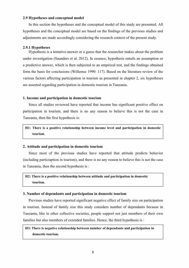
1. Income and participation in domestic tourism

Since all studies reviewed have reported that income has significant positive effect on

participation in tourism, and there is no any reason to believe this is not the case in

Tanzania, then the first hypothesis is:

2. Attitude and participation in domestic tourism

Since most of the previous studies have reported that attitude predicts behavior

(including particiaption in tourism), and there is no any reason to believe this is not the case

in Tanzania, then the second hypothesis is :

3. Number of dependants and participation in domestic tourism

Previous studies have reported significant negative effect of family size on participation

in tourism. Instead of family size this study considers number of dependants because in

Tanzania, like in other collective societies, people support not just members of their own

families but also members of extended families. Hence, the third hypothesis is :

H1: There is a positive relationship between income level and participation in domestic

tourism.

H2: There is a positive relationship between attitude and participation in domestic

tourism.

H3: There is negative relationship between number of dependants and participation in

domestic tourism.

9

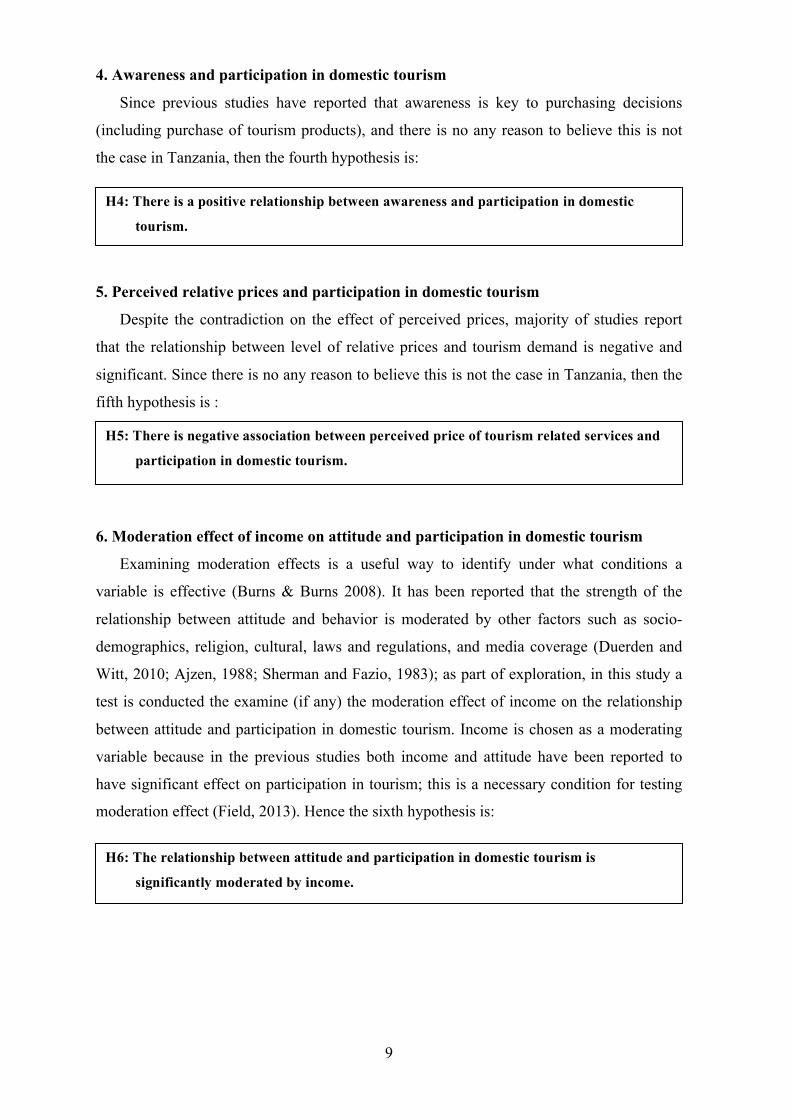
4. Awareness and participation in domestic tourism

Since previous studies have reported that awareness is key to purchasing decisions

(including purchase of tourism products), and there is no any reason to believe this is not

the case in Tanzania, then the fourth hypothesis is:

5. Perceived relative prices and participation in domestic tourism

Despite the contradiction on the effect of perceived prices, majority of studies report

that the relationship between level of relative prices and tourism demand is negative and

significant. Since there is no any reason to believe this is not the case in Tanzania, then the

fifth hypothesis is :

6. Moderation effect of income on attitude and participation in domestic tourism

Examining moderation effects is a useful way to identify under what conditions a

variable is effective (Burns & Burns 2008). It has been reported that the strength of the

relationship between attitude and behavior is moderated by other factors such as socio-

demographics, religion, cultural, laws and regulations, and media coverage (Duerden and

Witt, 2010; Ajzen, 1988; Sherman and Fazio, 1983); as part of exploration, in this study a

test is conducted the examine (if any) the moderation effect of income on the relationship

between attitude and participation in domestic tourism. Income is chosen as a moderating

variable because in the previous studies both income and attitude have been reported to

have significant effect on participation in tourism; this is a necessary condition for testing

moderation effect (Field, 2013). Hence the sixth hypothesis is:

H4: There is a positive relationship between awareness and participation in domestic

tourism.

H5: There is negative association between perceived price of tourism related services and

participation in domestic tourism.

H6: The relationship between attitude and participation in domestic tourism is

significantly moderated by income.

10

2.9.2 Conceptual model In this section the research hypotheses are visually displayed. The two figures below

are the conceptual models summarizing the six hypotheses of this study.

Figure 1: Main conceptual model

The figure above shows the predictor, predicted and control variables addressed in the

present study. Based on literature review the model illustrates the tentative direction and

signs of the relationships between social economic variables and participation in domestic

tourism (H 1 – H5).

Figure 2: Conceptual model the moderation test

Figure 2 illustrates the moderation effect of income on the relationship between

attiutude and participation in domestic tourism (H6). The model represents the influence of

income on the strength of attitude to predict participation in domestic tourism.

11

CHAPTER 3

METHODOLOGY

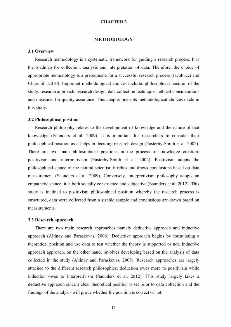
3.1 Overview

Research methodology is a systematic framework for guiding a research process. It is

the roadmap for collection, analysis and interpretation of data. Therefore, the choice of

appropriate methodology is a prerequisite for a successful research process (Iacobucci and

Churchill, 2010). Important methodological choices include: philosophical position of the

study, research approach, research design, data collection techniques, ethical considerations

and measures for quality assurance. This chapter presents methodological choices made in

this study.

3.2 Philosophical position

Research philosophy relates to the development of knowledge and the nature of that

knowledge (Saunders et al. 2009). It is important for researchers to consider their

philosophical position as it helps in deciding research design (Easterby-Smith et al. 2002).

There are two main philosophical positions in the process of knowledge creation:

positivism and interpretivism (Easterby-Smith et al. 2002). Positivism adopts the

philosophical stance of the natural scientist; it relies and draws conclusions based on data

measurement (Saunders et al. 2009). Conversely, interpretivism philosophy adopts an

empathetic stance; it is both socially constructed and subjective (Saunders et al. 2012). This

study is inclined to positivism philosophical position whereby the research process is

structured, data were collected from a sizable sample and conclusions are drawn based on

measurements.

3.3 Research approach

There are two main research approaches namely deductive approach and inductive

approach (Altinay and Paraskevas, 2008). Deductive approach begins by formulating a

theoretical position and use data to test whether the theory is supported or not. Inductive

approach approach, on the other hand, involves developing based on the analysis of data

collected in the study (Altinay and Paraskevas, 2008). Research approaches are largely

attached to the different research philosophies; deduction owes more to positivism while

induction owes to interpretivism (Saunders et al. 2012). This study largely takes a

deductive approach since a clear theoretical position is set prior to data collection and the

findings of the analysis will prove whether the position is correct or not.

12

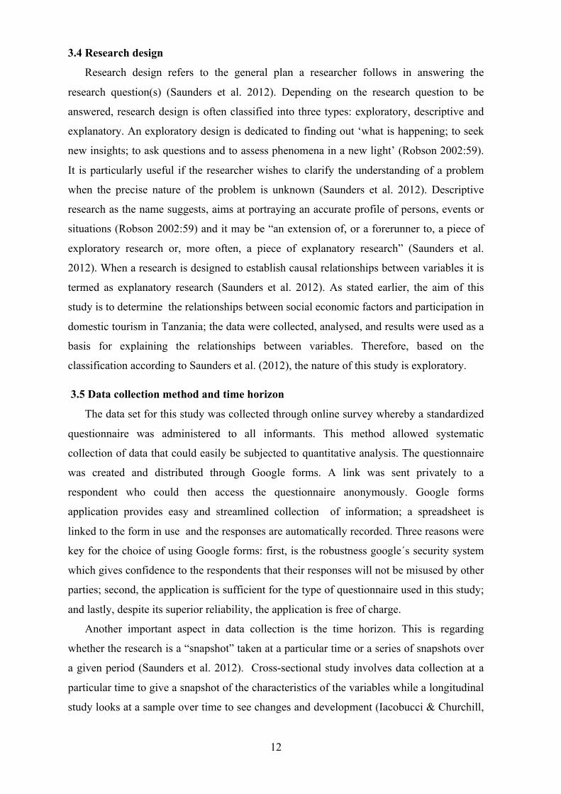
3.4 Research design

Research design refers to the general plan a researcher follows in answering the

research question(s) (Saunders et al. 2012). Depending on the research question to be

answered, research design is often classified into three types: exploratory, descriptive and

explanatory. An exploratory design is dedicated to finding out ‘what is happening; to seek

new insights; to ask questions and to assess phenomena in a new light’ (Robson 2002:59).

It is particularly useful if the researcher wishes to clarify the understanding of a problem

when the precise nature of the problem is unknown (Saunders et al. 2012). Descriptive

research as the name suggests, aims at portraying an accurate profile of persons, events or

situations (Robson 2002:59) and it may be “an extension of, or a forerunner to, a piece of

exploratory research or, more often, a piece of explanatory research” (Saunders et al.

2012). When a research is designed to establish causal relationships between variables it is

termed as explanatory research (Saunders et al. 2012). As stated earlier, the aim of this

study is to determine the relationships between social economic factors and participation in

domestic tourism in Tanzania; the data were collected, analysed, and results were used as a

basis for explaining the relationships between variables. Therefore, based on the

classification according to Saunders et al. (2012), the nature of this study is exploratory.

3.5 Data collection method and time horizon

The data set for this study was collected through online survey whereby a standardized

questionnaire was administered to all informants. This method allowed systematic

collection of data that could easily be subjected to quantitative analysis. The questionnaire

was created and distributed through Google forms. A link was sent privately to a

respondent who could then access the questionnaire anonymously. Google forms

application provides easy and streamlined collection of information; a spreadsheet is

linked to the form in use and the responses are automatically recorded. Three reasons were

key for the choice of using Google forms: first, is the robustness google´s security system

which gives confidence to the respondents that their responses will not be misused by other

parties; second, the application is sufficient for the type of questionnaire used in this study;

and lastly, despite its superior reliability, the application is free of charge.

Another important aspect in data collection is the time horizon. This is regarding

whether the research is a “snapshot” taken at a particular time or a series of snapshots over

a given period (Saunders et al. 2012). Cross-sectional study involves data collection at a

particular time to give a snapshot of the characteristics of the variables while a longitudinal

study looks at a sample over time to see changes and development (Iacobucci & Churchill,

13

2010). This study is cross-sectional since the relationships between variables are studied

based on data collected at a particular point in time. The choice of cross-sectional study is

justifiable considering the limited time frame that the study had to be accomplished.

3.6 Target population and sample selection

In most cases it is very difficult to collect data from the entire population intended for a

study; it is difficult, for example, to collect data from 45 millions people in Tanzania.

Researchers overcome this problem by collecting data from a small group of individuals

(sample) to represent the target population. In this study the target population are

Tanzanians who can be classified as potential tourists. This classification is made because

not everyone in a developing country like Tanzania can be considered as a potential tourist;

it is unreasonable to imagine, for example, a person living below absolute poverty line

would even think of travelling for leisure (in rich countries almost everyone can be

considered as a potential tourist).

But, even to identify those Tanzanians who can be regarded as potential tourists is a big

challenge because the national statistics bureau does not have a national database that

contains all demographic information such as occupations and income of all Tanzanians.

This makes it impossible to establish the relevant sampling frame for the intended study,

which means the use of probabilistic sampling techniques is limited. Due to that, the

present study has applied snowball sampling technique whereby an initial contact was

made with some prospective respondents and these respondents were asked to recommend

other potential participants (Altinay and Paraskevas, 2008). The link for the questionnaire

was sent to the initial respondents, after filling it they referred other potential respondents

who could then receive the link either through e-mail or Facebook private message.

3.7 Ethical considerations

Ethical consideration is an important aspect of a research process. Right from the

choice of research topic a researcher has to consider ethical implications of the study. The

general ethical guideline is that the research design should not subject research subjects to

embarrassment, harm or any other material disadvantage (Saunders et al. 2012). Generally

the nature of research questions and the design adopted for this study presented very low

risk for violating research ethics. All respondents participated in the study willingly; and in

addition, all the data were received anonymously and kept strictly confidential. All

respondents were guaranteed that their answers would not be treated individually instead

will be a part of aggregated dataset that would aid in the finding relationships between

variables under study.

14

3.8 Operationalization

3.8.1 Overview

After a thorough review of literature a standardized questionnaire was developed; this

was the main data collection instrument for this study. Following Saunders et al. (2012)

guidelines, the questionnaire was developed taking into consideration the conceptual

framework of the study. The questionnaire contained questions that probed all three types

of data variable as classified by Dillman (2007): opinion, behavior, and attribute data

variables. Opinion questions probed for the extent to which respondents agreed or

disagreed with given statements; while behavioral questions probed for what respondents

have engaged with (participation in different forms domestic tourism) and attribute

questions probed for the demographic characteristics of the respondents.

3.8.2 Validity of the questionnaire Instrument validity is an important aspect to consider when designing a questionnaire.

Saunders et al. (2012) reckons that a valid questionnaire will enable a researcher to collect

accurate data. Two measures were employed in this study to ensure validity of the

questionnaire. First, all the research questions were borrowed from various previous studies

and adjusted to suit the context of the present study. This was a preliminary measure to

ensure validity particularly of the multiple item constructs. The supervisor of this thesis and

some friends reviewed the first version of the questionnaire; their constructive comments

were incorporated into the final version of the questionnaire. Second, the questionnaire was

first sent to 5 individuals that were among potential respondents to check for the clarity and

relevance of the questions, feedback from all of them suggested that the questionnaire was

clear and relevant.

3.8.3 Measurement level of the variables Usefulness of the evidence obtained from research in part depends on the

operationalization of the constructs of interest into specific, concrete and measurable

variables (Burns & Burns 2008). The three types of data variables (opinion, behavior and

attribute variables) collected in this study had different levels of measurement. The level of

measurement expresses the relationship between what is being measured and the numbers

that represent what is being measured (Field, 2013). They can be classified as nominal,

ordinal, or scale (interval or ratio scale). Nominal variables appear in categories that cannot

be defined numerically or be ranked while ordinal variables are similar to nominal

variables except that the categories are ordered. Interval variable goes a step further ahead

of ordinal variable as the equal intervals on the scale represent equal differences in the

15

property being measured. Lastly ratio variables are those that in addition to meeting the

requirements of an interval variable, the ratios of the values along the scale should have a

true and meaningful zero point. Table 1 below summarizes all the variables used in this

study and their levels of measurement.

Table 1: Variables of the Conceptual Model VARIABLE ROLE TYPE

Participation Dependent variable Ratio variable

Income level Independent variable Ordinal variable

Attitude Independent variable Ordinal variable

Number of dependents Independent variable Ratio variable

Information (Awareness) Independent variable Ordinal variable

Perception of the relative prices Independent variable Ordinal variable

Age Control variable Ordinal variable

Gender, Marital status. Control variable Nominal variables

Participation In this study participation in domestic tourism is defined as the frequency of visiting

certain local tourist destinations. The variable was measured with a ratio scale whereby

respondents were given 8 destinations and were asked to state the number of times they

visited each of the destination. The total score for respondent´s participation was calculated

by adding the frequencies for those 8 activities. This approach for operationalization of

participation is a modification and reduction of the Leisure Participation Scale developed

by Ragheb and Griffith (1982) and Ragheb and Tate (1993). In previous studies, for

example Chiu and Kayat (2010), respondents were asked to state their participation during

the past six months; in this study respondents were asked to state their participation during

the last 12 months. This is reasonable because in Tanzania employees take annual leave at

different times during a year depending on the policy of the employers thus, using 12

months window is more sensible.

16

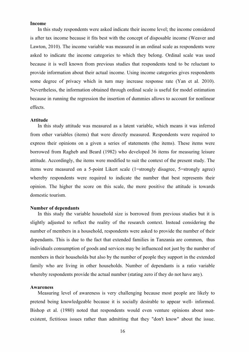
Income In this study respondents were asked indicate their income level; the income considered

is after tax income because it fits best with the concept of disposable income (Weaver and

Lawton, 2010). The income variable was measured in an ordinal scale as respondents were

asked to indicate the income categories to which they belong. Ordinal scale was used

because it is well known from previous studies that respondents tend to be reluctant to

provide information about their actual income. Using income categories gives respondents

some degree of privacy which in turn may increase response rate (Yan et al. 2010).

Nevertheless, the information obtained through ordinal scale is useful for model estimation

because in running the regression the insertion of dummies allows to account for nonlinear

effects.

Attitude In this study attitude was measured as a latent variable, which means it was inferred

from other variables (items) that were directly measured. Respondents were required to

express their opinions on a given a series of statements (the items). These items were

borrowed from Ragheb and Beard (1982) who developed 36 items for measuring leisure

attitude. Accordingly, the items were modified to suit the context of the present study. The

items were measured on a 5-point Likert scale (1=strongly disagree, 5=strongly agree)

whereby respondents were required to indicate the number that best represents their

opinion. The higher the score on this scale, the more positive the attitude is towards

domestic tourism.

Number of dependants In this study the variable household size is borrowed from previous studies but it is

slightly adjusted to reflect the reality of the research context. Instead considering the

number of members in a household, respondents were asked to provide the number of their

dependants. This is due to the fact that extended families in Tanzania are common, thus

individuals consumption of goods and services may be influenced not just by the number of

members in their households but also by the number of people they support in the extended

family who are living in other households. Number of dependants is a ratio variable

whereby respondents provide the actual number (stating zero if they do not have any).

Awareness Measuring level of awareness is very challenging because most people are likely to

pretend being knowledgeable because it is socially desirable to appear well- informed.

Bishop et al. (1980) noted that respondents would even venture opinions about non-

existent, fictitious issues rather than admitting that they "don't know" about the issue.

17

However, Sudman and Bradburn (1989) suggest that framing a question in terms of an

opinion statement reduces that risk; they suggest that respondents should not be asked

directly if they possess specific knowledge but should be asked in a softer format what their

opinion on the topic is. In this study the items for awareness construct were insipired by

Boo et al. (2009) who included awareness items in their model for determining destination

brand equity. However, the items were modified to suit the context of the present study.

Respondents were asked to indicate on a 5-point Likert scale the number that best

represents their opinion regarding their awareness of a given aspect of domestic tourism

(1=strongly disagree, 5=strongly agree). Therefore, awareness variable in the present study

is measured on an ordinal scale whereby higher the score represents higher level of

awareness about the aspects in question.

Perception of the relative prices In this study respondents were asked about their perception of the prices for goods and

services relevant for participation in domestic tourism- transport, accomodation, food and

drinks. The items for this construct were adopted from Boo et al. (2009). Like the other

constructs, the adopted items were adjusted to suit the context of the present study.

Therefore the measurement level of the relative price perception is ordinal whereby

respondents indicated on 5-point Likert scale their opinions regarding their perception the

state of prices for goods and services associated with domestic tourism (1=strongly

disagree, 5=strongly agree). The higher the score, the higher the perceived price of the

goods or services associated with domestic tourism.

Control variables: Age, gender and marital status All studies reviewed have included gender and marital status as binary variables (quite

understandable given their dichotomous nature); the age variable has been treated as either

numerical (example Alegre et al. 2013) or categorical variable (example: Kim et al. 2010).

As numerical variable means that respondents were required to report their age (in years)

while as categorical variable respondents are required to indicate certain age bracket to

which they belong. In this study, like previous studies, gender and marital status have been

treated as binary variables while the age variable has been treated as a categorical variable.

Age brackets were used instead of exact age in order to increase the response rate since in

Tanzania, like in most high context cultures, people do not like to disclose their age.

18

CHAPTER 4

CHOICE OF STATISTICAL ANALYSIS TECHNIQUES

4.1 Overview

In this chapter the choice of statistical techniques used to analyze the data is presented.

These techniques are useful in answering the research questions as they help to identify the

associations between variables. In particular, the techniques chosen are relevant for testing

the hypotheses stated in chapter 3. The data collected in this study have been analysed by

using IBM SPSS Statistics software version 21.0. This software package was chosen

because it has all the tools necessary to perform statistical measures intended in this study.

4.2 Descriptive Statistics

The analysis will begin with the presentation of descriptive statistics because these are

useful for summarizing large sets of data into simple and meaningful numbers (Aaker et al.

2011). The descriptive statistics include measurements such as means and standard

deviations and frequencies by categories. In case of the multiple scale items (attitude,

awareness and perception of relative prices) the assumption is that respondents understand

the scale values used in the survey as being equal distances apart (i.e. an interval scale). In

this way means and standard deviations on these constructs can be computed which

otherwise would not be valid if they were to be treated as ordinal scale (Stevens 1946).

4.3 Principal Component Analysis

In this study principal component analysis (PCA) is carried out for the multiple item

constructs (attitude, awareness and perception of relative prices) in order to group the

survey items into fewer and relevant components (Field, 2013). Performing principal

component analysis makes it possible to examine the convergent and divergent validity of

the constructs. PCA groups the items (set of responses to the survey statements for each

individual in the study) into factors that are not directly observable from the data.

Once factors have been extracted, it is possible to calculate the extent to which the

items load on these factors (Field, 2013). In order to discriminate between the factors, a

method called factor rotation is used. There are two types of factor rotation methods:

orthogonal rotation and oblique rotation. Orthogonal rotation is used when the researcher

has good theoretical reasons to assume that the factors are independent while oblique

rotation is used when the factors supposed to be related. Since in this study it is suspected

19

that there could be correlation between the identified variables, oblique rotation technique

will be applied. Furthermore, Costello and Osborne (2005) recommend using oblique

rotation because this method provides interpretable solution whether there is correlation

between the factors or not, while it is not the case for the orthogonal technique. SPSS has

two methods of oblique rotation- direct oblimin and promax; direct oblimi method will be

applied because acoording (Field, 2013) promax is a procedure designed for very large data

sets thus, not relevant for this study.

Three categories of output from the principal component analysis are examined. The

first category includes measures that examine if the correlations between items are suitable

for performing principal component analysis. These are: Kaiser-Meyer-Olkin (KMO)

measure of sampling adequacy, and Bartlett’s test of sphericity. KMO score below 0.6 and

Bartlett score whose significance level is above .05 indicates that principal component

analysis may not be the appropriate (Field, 2013). The second category include the

Eigenvalues of the identified factors; Kaiser’s criteria states that the number of factors

should be reduced to those with an Eigenvalue above one, that is those factors that account

for more of the total variance than one factor theoretically explains (Bryman and Cramer

2009). The third category of measures is provided in the pattern matrix. This matrix shows

a rotated solution of the factor loadings (partial correlations between the items and factors)

and will be used to interpret the factors. Stevens (2002, p.393) recommendation will be

followed, that is only items whose loading is greater than 0.512 will be considered for

further analysis.

4.4 Reliability analysis In order to validate the questionnaire the reliability of the multiple item scales was

checked. Reliability test measures the consistency of the construct under consideration

(Field, 2013). The reliabilty test for the three tentative constructs is conducted by assessing

a measure called Cronbach’s alpha. The maximum value of Cronbach’s alpha is 1, and the

higher value indicates the higher internal reliability (or higher internal consistency). Burns

and Burns (2008) suggest that the alpha must be at least .7 for the indicators to be internally

consistent. However, Kline (1999) notes that when dealing with pyschological constructs

such as attitude, values even below .7 can, realistically, be expected because of the

diversity of the constructs being measured. Nunnally (1978) suggests that in the early

stages of research, values even as low as .5 will suffice. In this study the threshold of alpha

at .7 will be considered.

20

4.5 Correlations

There will be a preliminary measure to assess the strength of the relationship between

the variables under the study; the correlations are analyzed using Pearson’s correlation

coefficient. The objective is just to get a feel of the potential relationships that exists

between the variables. The Pearson´s correlation coefficient ranges from -1 to 1, and the

further from 0, the stronger the linear association between the variables. A positive

correlation implies that increase in value in one variable is associated with increase in value

in the other variable. The correlations between the variables are presented in a correlation

matrix.

4.6 Multiple Regression

The conceptual model has been developed representing the hypotheses on the

relationship between social economic factors and participation in domestic tourism in

Tanzania. In order to test the model statistically, multiple linear regression analysis will be

deployed. Multiple linear regression analysis allows investigating if, and to what degree,

the independent variables (social economic factors) can significantly predict the dependent

variable (participation). The most common significance level at 5 % corresponding to a p-

value of .05 will be used. Significance level at 5% means that there is a 95% chance that

the results observed did not happen by chance (Saunders et al. 2012).

In order to run a valid multiple regression analysis, there are important assumptions that

must be met. The following four assumptions are the most important (Hair et al. 2010;

Field, 2013):

Independent errors

It is assumed that for any two observations the residual terms should be uncorrelated. If

this assumption is violated then the confidence intervals and significance tests will be

invalid (Field, 2013). However, estimates of the model parameters using the method of

least squares will still be valid but not optimal (Field, 2013). This assumption can be

diagnosed with the Durbin-Watson test, which tests for serial correlations between errors.

The test statistic varies between 0 and 4, whereby the middle value (2) means that the

residuals are uncorrelated. It is advised that the value of this test should be as close to 2 as

possible and values less than 1 or greater than 3 should raise concern (Field, 2013).

Linearity

Linearity an implicit assumption of all multivariate techniques based on correlational

measures of association (Hair et al. 2010). Since multiple regression analysis is based on

21

correlational measures, the relationship between the variables should be linear and it is a

problem if the dispersion of points indicates otherwise (Burns & Burns 2008). In this study

linearity is tested for each of the independent variables.

Homoscedasticity

Homoscedasticity means that at each level of the predictor variable(s), the variance of

the residual terms should be constant (Field, 2013). If the assumption of homoscedasticity

is violated then there is what is called heteroscedasticity. Violation of homoscedacity

assumption invalidates the confidence intervals and significance tests. However, estimates

of the model parameters using the method of least squares will still be valid but not optimal

(Field, 2013).

Normality of the error term distribution

It is assumed that the residuals in the model are random, normally distributed variables

with a mean of 0. It means that the differences between the model and the observed data

are most frequently zero or very close to zero and that the differences much greater than

zero happen only occasionally (Field, 2013). Hair et al. (2010) suggests that a better

diagnostic for this assumption is the use of normal probability plots. The normal

probability plot makes a straight diagonal line and the plotted residuals are compared with

the diagonal. If a distribution is normal, the residual line will closely follow the diagonal.

Multicollinearity

Multicollinearity is a problem that exists when there are high correlations between

some of the independent variables (Burns & Burns 2008). SPSS produces various

collinearity diagnotics; one of which is Variance Inflation Factor (VIF). This indicates

whether a predictor has a strong linear relationship with the other predictor(s). Some

general guidelines about what value of VIF are that: the VIF factor should not exceed 10,

and ideally should be close to one (Field, 2013).

Normal Distribution of the Variables

It is preferred that the dependent and independent variables are normally distributed,

especially for small sample sizes (Hardy & Bryman 2004). The skewness and kurtosis

diagnostics are useful in describing the shape of the distributions. Skewness describes the

extent to which the numbers are gathered at one end; whereas kurtosis refers to how close

together the points are, or the degree of peakedness. Positive values of skewness indicate

22

that scores are gathered on the left of the distribution, while negative values indicate a pile-

up on the right. Positive values of kurtosis indicate a peaked and heavy-tailed distribution,

while negative values indicate a flat and light-tailed distribution (Field, 2013). The further

the values of skewness and kurtosis, the more likely it is that the data are not normally

distributed (Burns & Burns 2008).

Regarding acceptable values, there various suggestion in the literature, for example

Weinberg & Abramowitz (2008) say that numbers that exceed +/- 2 are generally seen as

severely skewed while Field (2013) say that skewness and kurtosis should only be

considered in small samples but in large samples the researcher does not need to be worried

about normality. Since the subject of how big a sample is big enough is somehow

controversial, in this study skewness and kurtosis values produced by SPSS will be used to

compute statistic values (z) and check how significant these values are. The formulas for

statistic values (z) of skewness and kurtosis are borrowed from Hair et al. (2010) and given

as follows:

     𝑧!"#$%#!! =skewness

6𝑁

                                           𝑧!"#$%&'& =kurtosis

24𝑁

 

23

CHAPTER 5

PRELIMINARY ANALYSIS

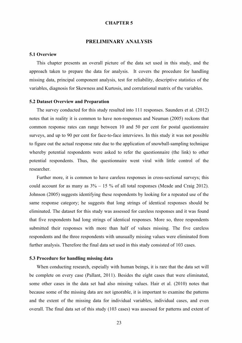
5.1 Overview

This chapter presents an overall picture of the data set used in this study, and the

approach taken to prepare the data for analysis. It covers the procedure for handling

missing data, principal component analysis, test for reliability, descriptive statistics of the

variables, diagnosis for Skewness and Kurtosis, and correlational matrix of the variables.

5.2 Dataset Overview and Preparation The survey conducted for this study resulted into 111 responses. Saunders et al. (2012)

notes that in reality it is common to have non-responses and Neuman (2005) reckons that

common response rates can range between 10 and 50 per cent for postal questionnaire

surveys, and up to 90 per cent for face-to-face interviews. In this study it was not possible

to figure out the actual response rate due to the application of snowball-sampling technique

whereby potential respondents were asked to refer the questionnaire (the link) to other

potential respondents. Thus, the questionnaire went viral with little control of the

researcher.

Further more, it is common to have careless responses in cross-sectional surveys; this

could account for as many as 3% – 15 % of all total responses (Meade and Craig 2012).

Johnson (2005) suggests identifying these respondents by looking for a repeated use of the

same response category; he suggests that long strings of identical responses should be

eliminated. The dataset for this study was assessed for careless responses and it was found

that five respondents had long strings of identical responses. More so, three respondents

submitted their responses with more than half of values missing. The five careless

respondents and the three respondents with unusually missing values were eliminated from

further analysis. Therefore the final data set used in this study consisted of 103 cases.

5.3 Procedure for handling missing data

When conducting research, espeially with human beings, it is rare that the data set will

be complete on every case (Pallant, 2011). Besides the eight cases that were eliminated,

some other cases in the data set had also missing values. Hair et al. (2010) notes that

because some of the missing data are not ignorable, it is important to examine the patterns

and the extent of the missing data for individual variables, individual cases, and even

overall. The final data set of this study (103 cases) was assessed for patterns and extent of

24

missing data, thanks to SPSS Missing Value Analysis application. According to Hair et al.

(2010), missing data under 10% for an individual case can generally be ignored, except

when the missing data occurs in a specific nonrandom pattern. In addition, the number of

cases with no missing data must be sufficient for the selected analysis technique if

replacement values will not be substituted. Figure 3(a) and 3(b) show the results of missing

value analysis conducted by SPSS.

Figure 3(a): Pie charts showing the extent of missing value in percentages

Figure 3(b): A plot showing the pattern of missing values

Figure 3(a) shows the extent of missing values in the data set. The figure shows that 10

out of 32 variables and 15 cases out of 103 had at least one missing value. The total number

of missing values was 17 out of 3296, which is 0.52% of the data set. SPSS did not produce

summary table because no variable had more than 10% missing values. Having determined

25

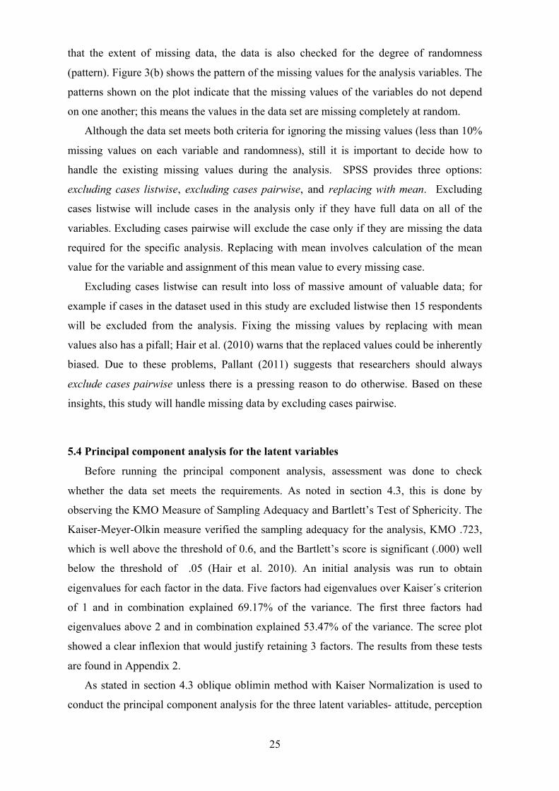
that the extent of missing data, the data is also checked for the degree of randomness

(pattern). Figure 3(b) shows the pattern of the missing values for the analysis variables. The

patterns shown on the plot indicate that the missing values of the variables do not depend

on one another; this means the values in the data set are missing completely at random.

Although the data set meets both criteria for ignoring the missing values (less than 10%

missing values on each variable and randomness), still it is important to decide how to

handle the existing missing values during the analysis. SPSS provides three options:

excluding cases listwise, excluding cases pairwise, and replacing with mean. Excluding

cases listwise will include cases in the analysis only if they have full data on all of the

variables. Excluding cases pairwise will exclude the case only if they are missing the data

required for the specific analysis. Replacing with mean involves calculation of the mean

value for the variable and assignment of this mean value to every missing case.

Excluding cases listwise can result into loss of massive amount of valuable data; for

example if cases in the dataset used in this study are excluded listwise then 15 respondents

will be excluded from the analysis. Fixing the missing values by replacing with mean

values also has a pifall; Hair et al. (2010) warns that the replaced values could be inherently

biased. Due to these problems, Pallant (2011) suggests that researchers should always

exclude cases pairwise unless there is a pressing reason to do otherwise. Based on these

insights, this study will handle missing data by excluding cases pairwise.

5.4 Principal component analysis for the latent variables

Before running the principal component analysis, assessment was done to check

whether the data set meets the requirements. As noted in section 4.3, this is done by

observing the KMO Measure of Sampling Adequacy and Bartlett’s Test of Sphericity. The

Kaiser-Meyer-Olkin measure verified the sampling adequacy for the analysis, KMO .723,

which is well above the threshold of 0.6, and the Bartlett’s score is significant (.000) well

below the threshold of .05 (Hair et al. 2010). An initial analysis was run to obtain

eigenvalues for each factor in the data. Five factors had eigenvalues over Kaiser´s criterion

of 1 and in combination explained 69.17% of the variance. The first three factors had

eigenvalues above 2 and in combination explained 53.47% of the variance. The scree plot

showed a clear inflexion that would justify retaining 3 factors. The results from these tests

are found in Appendix 2.

As stated in section 4.3 oblique oblimin method with Kaiser Normalization is used to

conduct the principal component analysis for the three latent variables- attitude, perception

26

of relative prices and awareness. The constructs identified and validated here will finally be

included in the procedures for testing hypotheses. Among the output tables of this analysis,

it is common to interpret the results of the pattern matrix. However, there situations in

which values in the pattern matrix are suppressed because of the relationship between the

factors therefore another output table called structure matrix is a useful double check

(Field, 2013). Since SPSS produces these output tables simultaneously, both, the pattern

matrix and the structure matrix are presented in the following table.

Table 2: Principal Component Analysis (n=103)

Extraction Method: Principal Component Analysis. Rotation Method: Oblimin with Kaiser Normalization.a a. Rotation converged in 8 iterations.

From the table above, both the pattern matrix and the structure matrix show that three

factors have been extracted where all items are well above Stevens (2002, p.393) threshold

of 0.512 in their respective components except ATT1 and ATT5. Being below the

27

threshold means that these two items diverged from other items in the same component.

The question for ATT1 was I think visiting tourist attractions in my country is a wise use of

time and that for ATT5 was I think visiting various local tourist attractions is important to

me. Looking at the responses these two items had an average of 4.07 and 4.26

respectively, out of the maximum 5; among the remaining items the average was 3.52 or

below. Different from the other questions in this component, questions ATT1 And ATT5

aimed at measuring the extent to which respondents think participating in domestic tourism

is a sensible, essential or a prudent practice. One possible explanation for the distinct

higher average scores for ATT1 and ATT2 is that may be the use of the words “wise” and

“important” made respondents feel that if they are “reasonable” then they are expected to

support these statements. The tendency of respondents giving socially desirable answers

rather than their true opinion is a common problem in surveys Dillman (2007). With

respect to the threshold therefore, these two items are dropped.

5.5 Reliabilty analysis

As stated in section 4.4 the internal consistency of the constructs has been assessed by

determining the Cronbach’s Alpha (α). The subscales for attitude towards domestic

tourism, awareness about aspects of domestic tourism and perception of relative prices all

had high reliabilities, well above the threshold of .7. Table 6.2 below presents the

Cronbach’s Alphas for the constructs.

Table 3: Cronbach’s Alphas for the Constructs

Construct Cronbach’s

Alpha Number of Items

Valid cases

Excluded cases

Total cases

Attitude towards domestic tourism 0.842 7 100 3 103

Awareness 0.793 6 97 6 103

Perception of relative prices 0.912 3 103 0 103

28

5.6 Descriptive Statistics: categorical variables After excluding the 5 cases with long strings of identical responses, and 3 cases with

excessively missing values, the final data set had 103 cases. The table below presents

categorical variables for the cases included for final analysis.

Table 4: Descriptive Statistics of the Categorical Variables

Variable Categories Frequency Percent Cumulative Percent

Gender Female 41 39.8 39.8 Male 62 60.2 100

Marital status Single 53 51.5 51.5 Married/Cohabiting 50 48.5 100

Age

Below 20 0 0 0 20-30 46 44.7 44.7 31-40 51 49.5 94.2 41-50 4 3.9 98.1 Above 50 2 1.9 100

Income

Below Tzs. 500000 12 11.7 11.7 Tzs. 500000-1000000 26 25.2 36.9 Tzs. 1000000-2000000 33 32.0 68.9 Tzs. 2000000-3000000 16 15.5 84.5 Tzs. 3000000-4000000 7 6.8 91.3 Tzs . 4000000-5000000 4 3.9 95.1 Above Tzs. 5000000 5 4.9 100

The table above shows differences in demographic attributes among respondents.

Considering the gender of the respondents, the sample contains more males (62) than

females (41). None of the respondents was below 20 years while majority of the

respondents (97) were either 20 – 30 or 31 -40 years old; only 6 respondents were either 41

– 50 or above 50 years old. Income distribution seem to concentrate on the incomes

ranging from Tzs. 500000 to Tzs. 3000000 (75 respondents) individuals with income below

Tzs. 500000 are just 12 and those above Tzs. 3000000 are 16.

This distribution can partly be explained by the biasness of the snowball sampling

technique (Altinay and Paraskevas, 2008). When initial respondents are asked to refer to

other potential respondents, they are most likely to identify other potential respondents who

are similar to themselves, resulting in a sample where majority of the respondents have

more or less similar characteristics (Lee 1993). Due to scanty representation of some

categories in age and income variables, during the analysis the data for these variables will

be re-categorised to obtain fewer and more manageable caterigories.

29

5.6 Descriptive statistics: constructs and ratio variables

In this section presents the descriptive statistics for the three constructs (particiaption,

awareness and perception of relative prices) and the ration variables (participation and

number of dependants). The scores presented for the constructs (factors) are based on the

the averages of the item responses. The table below presents the descriptive statistics for

the constructs and ratio variables.

Table 5: Descriptive Statistics for the Constructs and Ratio Variables

Variable Mean SD Minimum Maximum N

Participation in domestic tourism 4.00 2.11 0 8 103

Attitude towards domestic tourism 3.46 0.58 2.29 4.57 103

Awareness 3.42 0.59 2.00 4.83 103

Perception of relative prices 3.14 1.15 1.00 5.00 103

Number of dependants 2.82 1.94 0 8 100

The table above presents useful information on the opinions, behavior and attributes of

the respondents that were involved in this study. Starting with participation, the data shows

that the average score is 4, out of the maximum 8, and the minimum and maximum values

indicate that there is at least one respondent who have not visited any of the given tourist

destination. Therefore, the mean value may not be a good measure to make conclusion

regarding respondents´ participation in domestic tourism; after all, mean values are known

to be vulnerable to the influence of extreme values in the data set (Field, 2013).

Further more, the table shows that attitude has a mean score of 3.46 out of the

maximum 5. The minimum attitude score is 2.29, which imply negative attitude towards

domestic tourism while the highest score is 4.57, which imply quite positive attitude

towards domestic tourism. On this scale an average score of 3.0 would imply that

respondents have a “neutral attitude” towards domestic tourism. Neutral position is difficult

30

to interpret because they may reflect many different meanings such as “neither agree nor

disagree”, “undecided”, “don’t know”, and “no opinion” (Raaijmakers, et al., 2000). The

information provided in this table is not sufficient to draw conclusions regarding

respondents´ attitude towards domestic tourism.

More so, the table shows that awareness has a mean score of 3.42 out of the maximum

5. The minimum awareness score is 2.00, which imply low level of awareness about

important aspects for participation in domestic tourism, while the maximum score is 4.83,

which imply quite high level of awareness about important aspects for participation in

domestic tourism. Perception of relative prices has a mean score of 3.14 out of the

maximum 5. The minimum score for perception of relative prices is 1 implying that one or

more respondents surveyed in this study believe that the prices of services at tourist

destinations are not very high. However, the maximum score is 5 implying that one or more

respondents believe that the prices of services at tourist destinations are very high. The

information presented in this table is not sufficient to draw conclusions regarding

respondents´ level of awareness about important aspects for participation in domestic

tourism and their perceptions about the prices of services at tourist destinations.

Finally the table presents information about respondents´ number of dependants. On

average respondents have 2.82 depents (approximately 3). However the minimum value of

0 shows there are one or more respondents who do not have dependants at all while the

maximum value of 8 shows that there is at least one respondent with 8 dependants. The

presence of at least one respondent without dependants can be explained by the fact that the

sample contains a big chunk of individuals between 20 and 30 years old; in most cases

these are individuals who have just established themselves therefore it is not common for

them to start immediately helping other family members (including extended family

members).

As noted for all the variables, the descriptive statistics provided in Table 5 are not

sufficient to draw meaningful conclusions about the opinions, behavior and attributes of the

respondents surveyed in this study. Even for those variables where partial explanation has

been provided, further tests are required to get deeper insights; this is performed in the

analysis chapter.

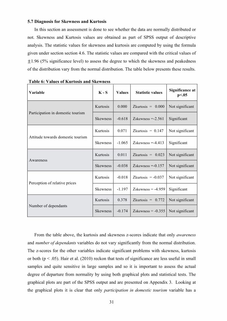
31

5.7 Diagnosis for Skewness and Kurtosis

In this section an assessment is done to see whether the data are normally distributed or

not. Skewness and Kurtosis values are obtained as part of SPSS output of descriptive

analysis. The statistic values for skewness and kurtosis are computed by using the formula

given under section section 4.6. The statistic values are compared with the critical values of

±1.96 (5% significance level) to assess the degree to which the skewness and peakedness

of the distribution vary from the normal distribution. The table below presents these results.

Table 6: Values of Kurtosis and Skewness

Variable K - S Values Statistic values Significance at p<.05

Participation in domestic tourism Kurtosis 0.000 Zkurtosis = 0.000 Not significant

Skewness -0.618 Zskewness =-2.561 Significant

Attitude towards domestic tourism Kurtosis 0.071 Zkurtosis = 0.147 Not significant

Skewness -1.065 Zskewness =-4.413 Significant

Awareness Kurtosis 0.011 Zkurtosis = 0.023 Not significant

Skewness -0.038 Zskewness =-0.157 Not significant

Perception of relative prices Kurtosis -0.018 Zkurtosis = -0.037 Not significant

Skewness -1.197 Zskewness = -4.959 Significant

Number of dependants Kurtosis 0.378 Zkurtosis = 0.772 Not significant

Skewness -0.174 Zskewness = -0.355 Not significant

From the table above, the kurtosis and skewness z-scores indicate that only awareness

and number of dependants variables do not vary significantly from the normal distribution.

The z-scores for the other variables indicate significant problems with skewness, kurtosis

or both (p < .05). Hair et al. (2010) reckon that tests of significance are less useful in small

samples and quite sensitive in large samples and so it is important to assess the actual

degree of departure from normality by using both graphical plots and statistical tests. The

graphical plots are part of the SPSS output and are presented on Appendix 3. Looking at

the graphical plots it is clear that only participation in domestic tourism variable has a

32

shape close to normal distribution. Perception of relative prices and attitude towards

domestic tourism variables appear to be quite skewed even graphically.

Since normality is important criteria for correlational-based analyses, the problems

identified here have to be addressed before proceeding with regression analysis (Hair et al.

2010). There are four methods for correcting problems with the data (Field, 2013). The first

method is to trim the data, under this method certain amounts of scores are deleted from the

extremes. The second method is called winsorizing whereby outliers are substituted with

highest values that are not outliers. The third method is to analyse the data with robust

methods, which typically involves a technique known as bootstrapping. Robust tests

provide estimate statistics that are reliable even when the normal assumptions of the

statistic are not met. And the fourth method is to transform the data. Pointing at the

shortfalls of trimming the data, winsorizing and data transformation, Field (2013) suggests

that, among the four methods, analyzing data with robust tests is the best. Since SPSS

provides bootstrap option for most of the procedures, this study will follow Field´s (2013)

recommendation and use robust methods to address the problems of skewness and kurtosis.

5.8 Correlation matrix

Before running the regression, it is important to get a rough idea of the relationships

between predictors and the outcome (Hair et al., 2010). In this section the results of

bootstrapped correlational analysis are presented. The Pearson´s correlation coefficients

between every pair of variables is useful not only just for getting a rough idea of the

relationships but also for preliminary assessment of multicollinearity. If multicolinearity is

absent then there should be no substantial correlations between predictors Field (2013)

suggests a threshold of r ≤ .9.

More so, due to lack of normality in some of the variables, then according to Field

(2013) it is important to be more concerned with the bootstrapped confidence intervals than

the significance levels per se. This is because significance might be affected by the

distribution of scores, but confidence intervals are not. A confidence interval of correlation

coefficient that crosses zero means that the population value could actually be zero, which

means it is possible that there is no effect at all between the variables. Table 7 presents the

results of the correlation analysis for the interval and ratio variables.

33

Table 7: Results of Correlation Analysis.

1 2 3 4 5

1. PARTICIPATION 1

2. ATTITUDE .426**

[.196, .627] 1

3. AWARENESS .147

[-.032, .310]

.114

[-.072, .297] 1

4. PRICE_PERCEPTION -.432**

[-.579, -.259]

-.279**

[-.468, -.077]

-.239*

[-.406, -.052] 1

5. DEPENDANTS -.347**

[-.530, -.164]

-.190

[-.349, -.025]

-.068

[-.246, .131]

-.097

[-.293, .107] 1

Note:

1. ** Correlation is significant at the 0.01 level (2-tailed).

2. * Correlation is significant at the 0.05 level (2-tailed).

3. Bootstrap results are based on 1000 bootstrap samples.

4. BCa bootstrap 95% confidence intervals are reported in brackets.

The table above shows that PARTICIPATION is significantly correlated with

ATTITUDE (r= .426), PRICE_PERCEPTION (r= -.432) and DEPENDANTS (r= -.347) all

at 0.01 significant level. This is also confirmed by confidence intervals (95%) that do not

cross zero (lower and upper limits have the same signs). However, PARTICIPATION is

not significantly correlated with AWARENESS (r= .147); this is confirmed by the

confidence interval that crosses zero, which indicates that the value of correlation value

could actually be zero (no effect between the variables). This is an early alarm that

AWARENESS may not have significant effect in the regression model.

More so, the table shows that only PRICE_PERCEPTION has significant relationship

with two other predictor variables: ATTITUDE, at 0.01 significant level, and

AWARENESS at 0.05 significant level. The rest of the predictor variables do not have

significant correlations, which is a good indication for absence of multicollinearity.

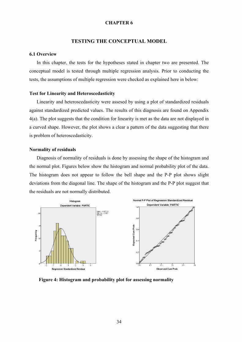
34

CHAPTER 6

TESTING THE CONCEPTUAL MODEL

6.1 Overview

In this chapter, the tests for the hypotheses stated in chapter two are presented. The

conceptual model is tested through multiple regression analysis. Prior to conducting the

tests, the assumptions of multiple regression were checked as explained here in below:

Test for Linearity and Heteroscedasticity

Linearity and heteroscedasticity were assesed by using a plot of standardized residuals

against standardized predicted values. The results of this diagnosis are found on Appendix

4(a). The plot suggests that the condition for linearity is met as the data are not displayed in

a curved shape. However, the plot shows a clear a pattern of the data suggesting that there

is problem of heteroscedasticity.

Normality of residuals

Diagnosis of normality of residuals is done by assessing the shape of the histogram and

the normal plot. Figures below show the histogram and normal probability plot of the data.

The histogram does not appear to follow the bell shape and the P-P plot shows slight

deviations from the diagonal line. The shape of the histogram and the P-P plot suggest that

the residuals are not normally distributed.

Figure 4: Histogram and probability plot for assessing normality

35

Multicollinearity

Variance inflation factors (VIF) and tolerance statistics are used to quantify the severity

of multicollinearity. The results of this diagnosis are found on Appendix 4(b). The VIF

values are all well below 10 but some of tolerance statistics are well below 0.2, and the

average VIF is 1.7 which is greater than 1 (the threshold); therefore, it is fair that conclude

that multicollinearity may be problem in the data set.

Checking for outliers

Partial plots are used to detect the outliers. These are scatterplots of the residuals of the

outcome variable and each of the predictors when both variables are regressed separately

on the remaining predictors. Outliers on a partial plot represent cases that might have undue

influence on a predictor´s regession coefficient. Partial plots for the data set of this study

are found on Appendix 4(c). All partial plots do not indicate presence of obvious outliers,

the dots are more or less evenly spread.

In conclusion, the summary of the assessment of the multiple regression assumptions is

presented in the table below.

Table 8: Summary on the Assessment of the Multiple Regression Assumptions Assumption Finding EVIDENCE

Linearity Meets requirements Appendix 7.1a

Heteroscedasticity Requirements not met Appendix 7.1a

Multicollinearity Requirements not met Appendix 7.1b

Normality of residuals Requirements not met Figure 7.1

Outliers Meets requirements Appendix 7.1c

The table above shows that not all assumptions for multiple regression analysis are met.

This is not a surprise; snowball-sampling technique has an inherent biasness that can hardly

produce data that meet all assumptions of multiple regression analysis (Altinay and

Paraskevas, 2008).

6.2 Defining new categories for age and income variables

In the original data set there were five age categories and seven income categories. The

objective for providing many categories was to increase the precision of the data collected.

However, as shown in Table 4, certain categories were barely represented in the data, for

example none of the respondents was below 20 years old. Therefore, it is necessary to

transform the data into new categories of age and income before testing the hypotheses.

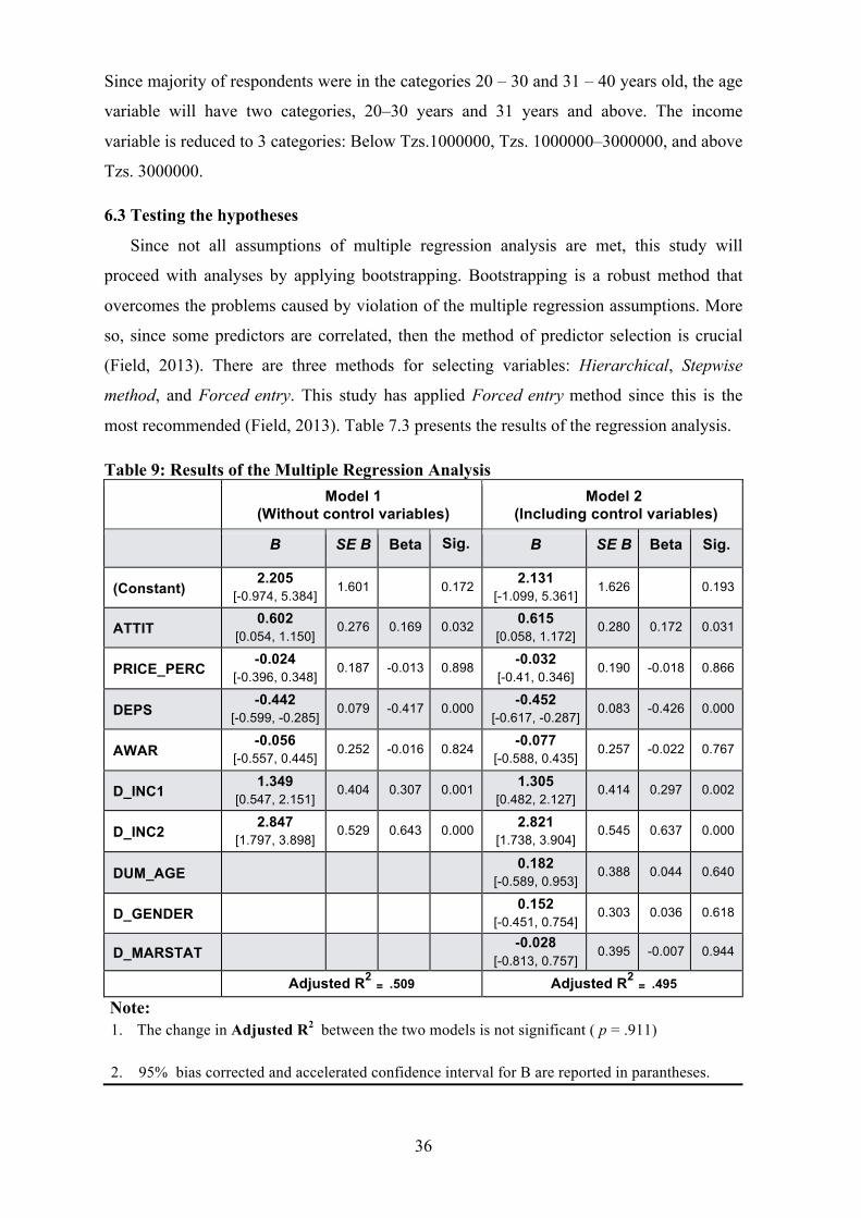
36

Since majority of respondents were in the categories 20 – 30 and 31 – 40 years old, the age

variable will have two categories, 20–30 years and 31 years and above. The income

variable is reduced to 3 categories: Below Tzs.1000000, Tzs. 1000000–3000000, and above

Tzs. 3000000.

6.3 Testing the hypotheses

Since not all assumptions of multiple regression analysis are met, this study will

proceed with analyses by applying bootstrapping. Bootstrapping is a robust method that

overcomes the problems caused by violation of the multiple regression assumptions. More

so, since some predictors are correlated, then the method of predictor selection is crucial

(Field, 2013). There are three methods for selecting variables: Hierarchical, Stepwise

method, and Forced entry. This study has applied Forced entry method since this is the

most recommended (Field, 2013). Table 7.3 presents the results of the regression analysis.

Table 9: Results of the Multiple Regression Analysis

Model 1

(Without control variables) Model 2

(Including control variables)

B SE B Beta Sig. B SE B Beta Sig.

(Constant) 2.205

[-0.974, 5.384] 1.601 0.172 2.131 [-1.099, 5.361] 1.626

0.193

ATTIT 0.602

[0.054, 1.150] 0.276 0.169 0.032 0.615

[0.058, 1.172] 0.280 0.172 0.031

PRICE_PERC -0.024

[-0.396, 0.348] 0.187 -0.013 0.898 -0.032 [-0.41, 0.346] 0.190 -0.018 0.866

DEPS -0.442

[-0.599, -0.285] 0.079 -0.417 0.000 -0.452 [-0.617, -0.287] 0.083 -0.426 0.000

AWAR -0.056

[-0.557, 0.445] 0.252 -0.016 0.824 -0.077 [-0.588, 0.435] 0.257 -0.022 0.767

D_INC1 1.349

[0.547, 2.151] 0.404 0.307 0.001 1.305

[0.482, 2.127] 0.414 0.297 0.002

D_INC2 2.847

[1.797, 3.898] 0.529 0.643 0.000 2.821

[1.738, 3.904] 0.545 0.637 0.000

DUM_AGE 0.182

[-0.589, 0.953] 0.388 0.044 0.640

D_GENDER 0.152

[-0.451, 0.754] 0.303 0.036 0.618

D_MARSTAT -0.028

[-0.813, 0.757] 0.395 -0.007 0.944

Adjusted R2 = .509 Adjusted R2 = .495

Note: 1. The change in Adjusted R2 between the two models is not significant ( p = .911) 2. 95% bias corrected and accelerated confidence interval for B are reported in parantheses.

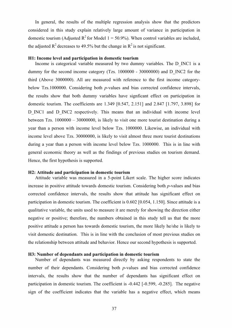
37

In general, the results of the multiple regression analysis show that the predictors

considered in this study explain relatively large amount of variance in participation in

domestic tourism (Adjusted R2 for Model 1 = 50.9%). When control variables are included,

the adjusted R2 decreases to 49.5% but the change in R2 is not significant.

H1: Income level and participation in domestic tourism Income is categorical variable measured by two dummy variables. The D_INC1 is a

dummy for the second income category (Tzs. 1000000 - 30000000) and D_INC2 for the

third (Above 3000000). All are measured with reference to the first income category-

below Tzs.1000000. Considering both p-values and bias corrected confidence intervals,

the results show that both dummy variables have signficant effect on participation in

domestic tourism. The coefficients are 1.349 [0.547, 2.151] and 2.847 [1.797, 3.898] for

D_INC1 and D_INC2 respectively. This means that an individual with income level

between Tzs. 1000000 – 30000000, is likely to visit one more tourist destination during a

year than a person with income level below Tzs. 1000000. Likewise, an individual with

income level above Tzs. 30000000, is likely to visit almost three more tourist destinations

during a year than a person with income level below Tzs. 1000000. This is in line with

general economic theory as well as the findings of previous studies on tourism demand.

Hence, the first hypothesis is supported.

H2: Attitude and participation in domestic tourism Attitude variable was measured in a 5-point Likert scale. The higher score indicates

increase in positive attitude towards domestic tourism. Considering both p-values and bias

corrected confidence intervals, the results show that attitude has significant effect on

participation in domestic tourism. The coefficient is 0.602 [0.054, 1.150]. Since attitude is a

qualitative variable, the units used to measure it are merely for showing the direction either

negative or positive; therefore, the numbers obtained in this study tell us that the more

positive attitude a person has towards domestic tourism, the more likely he/she is likely to

visit domestic destination. This is in line with the conclusion of most previous studies on

the relationship between attitude and behavior. Hence our second hypothesis is supported.

H3: Number of dependants and participation in domestic tourism Number of dependants was measured directly by asking respondents to state the

number of their dependants. Considering both p-values and bias corrected confidence

intervals, the results show that the number of dependants has significant effect on

participation in domestic tourism. The coefficient is -0.442 [-0.599, -0.285]. The negative

sign of the coefficient indicates that the variable has a negative effect, which means

38

increase in one dependant reduces participation by 0.442 times (his coeffiecient that the is

meaningful when a person has at least three dependants- 3 x 0.442 = 1.326). The significant

negative effect of the number of dependants is in line with the findings of previous studies;

hence, the third hypothesis is supported.

H4: Awareness and participation in domestic tourism Awareness variable was measured in a 5-point Likert scale. The higher score indicates

higher level of awareness about various aspects relevant for participation in domestic

tourism. Considering both p-values and bias corrected confidence intervals, our results

show that level of awareness does not have significant effect on participation in domestic

tourism. The coefficient is -0.056 (p=0.767); the confidence interval crosses zero [-0.557,

0.445] indicating that the value of the coefficient for awareness could be even zero (no

effect). Therefore, the numbers obtained in this study tell us that change in the level of

awareness does not impart one´s participation in domestic tourism. The expectation, based

on marketing theory, was that increase in awareness would significantly increase

participation in domestic tourism. Hence, our hypothesis is not supported.

H5: Perception of relative prices and participation in domestic tourism. Perception of relative prices was measured in a 5-point Likert scale. The higher the

score indicates the stronger the opinion that prices at tourism destinations are very high

Considering both p-values and bias corrected confidence intervals, the results show that

perception of relative prices does not have significant effect on participation in domestic

tourism. The coefficient is -0.024 (p=0.866); the confidence interval crosses zero [-0.396,

0.348] indicating that the value of the coefficient for perception of relative prices could be

even zero (no effect). Therefore, the numbers obtained in this study tell us that how a

person perceives prices at the tourist destination does not impart their participation in

domestic tourism. The expectation, based on previous studies, was that the stronger a

person believes prices at domestic tourist destinations are very high, the lower would be

their rate of participation in domestic tourism; hence, the fifth hypothesis is not supported.

The effect of control variables The results of the analysis indicate that the overall effect all control variables is not

significant. When control variables are included in the model, change in the value of R2 is

insignificant (p = .911). Likewise, none of individual control variables has significant

effect: age (p=0.640), the confidence interval is [-0.589, 0.953]; gender (p=0.618), the

confidence interval is [-0.451, 0.754]; and marital status (p=0.944), the confidence interval

is [-0.813, 0.757]. Hence, considering both the significance values and the confidence

39

intervals, the results suggest that the effect of age, marital status and gender on

participation in domestic tourism is insignificant.

H6: Moderation effect of income on attitude and participation in domestic tourism The results on table 9 do not give information about the moderation effect of income on

the relationship between attitude and domestic tourism; thus, a separate test for moderation

effect is run. SPSS does not have in-built application for testing moderation effects but

thanks to Prof. Andrew F. Hayes at Ohio State University who developed an application

called PROCESS that can be installed into SPSS and facilitate this test. PROCESS is

available for free on Hayes´s website. Since the moderating variable (income) has three

categories, the test is run twice to test the effect of the two dummy variables. The variables

are for income level Tzs. 1000000 – 3000000 and income bove Tzs. 3000000; both are

measured with reference to income below Tzs. 1000000. The results of the test for

moderation are presented in Tables 10 and 11.

Table 10: Moderation effect of Income Level Tzs. 1000000 - 3000000

The moderating effect of income on the relationship between attitude (X) and

participation (Y) is shown in the lower section of the table (Conditional effect of X on Y).

The results show that when income is lower than Tzs. 1000000, then attitude does not have

40

significant effect on participation in domestic tourism: effect = .67; 95% CI [-.2609,

1.5943] ; and p= .157. However, when income level is between Tzs. 1000000 and 3000000,

the relationship between attitude and participation in domestic tourism becomes

significantly positive: effect = 2.11; 95% CI [.1390, 4.0838] ; and p= .036. This means that

change of income to a level between Tzs. 1000000 and 3000000 has a significant effect on

the strength of the relationship between attitude and participation in domestic tourism.

Table 11: Moderation Effect of Income Level Above Tzs. 3000000

The moderating effect of income on the relationship between attitude (X) and

participation (Y) is shown in the lower section of the table (Conditional effect of X on Y).

The results show that when an person has income lower than Tzs. 1000000 then attitude

does not have significant effect on participation in domestic tourism: effect = -.21; 95% CI

[-1.4784, 1.0558] and p= .741. However, when income level is above Tzs. 3000000, the

relationship between attitude and participation in domestic tourism becomes positive and

significant : effect = 2.02; 95% CI [1.0942, 2.9526], p= .000.

41

CHAPTER 7

DISCUSSION

7.1 Overview

The usefulness of data analysis is on its ability to help researchers make sense of the

data collected. The analyses performed in the previous chapter have provided answers to

the six hypotheses of this study. Some of the hypotheses were supported while others were

not. In this chapter the results of the analyses are discussed and important insights are

drawn.

7.2 Income level and participation in domestic tourism

The results of the analyses show that the relationship between income and participation

in domestic tourism is significantly positive. The results suggest that if other factors remain

constant, then individuals who belong to a higher income class will participate in domestic

tourism more often than individuals in a lower income class. This is not a surprising insight

because there are tons of previous studies that confirm the same. For example Seddighi and

Shearing (1997) and Garin-Munoz (2009) also found that income is one of the main

determinants of domestic tourism in Northumbria (UK) and Galicia (Spain) respectively.

Therefore, the findings of this study and those of other studies on tourism demand

consistently reaffirm what economists have known for centuries namely the influence of

income on demand for goods and services.

However, Weaver and Lawton (2010) emphasize that income is the most important

economic factor associated with increased tourism demand; Bigano et al. (2006) also found

that even though income is a significant determinant of tourism demand, its impact is even

much more noticeable in low income countries (say, like Tanzania). Having found in this

study that income has significant relationship with participation in domestic tourism, it

seemed worthwhile to explore and get deeper insights from the data collected. This was

achieved by conducting a post hoc test called Tukey’s Studentized Range (HSD) to

measure how participation in domestic tourism in Tanzania changes as income moves from

one class to another.

The results of this test (presented in appendix 5) show that any increase in income from

the level Tzs. 1000000-3000000 to above Tzs. 3000000 increased participation much more

compared to increase in income from below Tzs. 1000000 to Tzs. 1000000-3000000. This

implies that if the respondents in this study get any increase in income their participation in

42

domestic tourism will increase, but that increase would be even much more noticeable if

the income goes above Tzs. 3000000.

7.3 Attitude and participation in domestic tourism

The results of the test on the relationship between attitude and participation in domestic

tourism turned out significantly positive. Thus, the results support the second hypothesis of

this study. This too was not a surprise because researchers in marketing have repeatedly

confirmed the influence of attitudes on the purchase of goods and services and tourism

products are surely not exception to that. However, the results of this study are important

because they provide empirical evidence in a context different from the contexts where

most of the studies on the relationship between attitude and participation in tourism have

been conducted. To the best of my knowledge, no similar study has been conducted in

Tanzania, therefore the findings not only reaffirm the universality of the theory of attitude

and consumer behavior but also provide useful insights relevant for marketers of tourism

products in Tanzania (This will be discussed in detail on the implications of the study).

Another interesting aspect on the relationship between attitude and participation in

domestic tourism (in Tanzania) is the moderation effect of income. The results of the

moderation test indicate that attitude is positively and significantly related to participation

when income level is higher. In other words, the results predict that if an individual has low

income then positive attitude alone will not result into high participation in domestic

tourism. It is interesting because in most cases when government officials and tourism

practitioners in Tanzania speak about the low incidence of domestic tourism, they often

refer to negative attitude as if it is the only factor hindering participation in domestic

tourism. The results of this study indicate that while attitude is a significant predictor of

participation in domestic tourism, its impact depends also on the incomes of individuals.

More interesting insight revealed by this study is the level of attitude among

respondents who participated in this study. As mentioned earlier it is common to hear

people attributing low incidence of domestic tourism in Tanzania to negative attitudes, to

the best of my knowledge, most of those who make this claim do not have any empirical

evidence to back up their statements. Even Mariki et al. (2011), who explored the factors

affecting domestic tourism in northern Tanzania, did not actually measure attitudes but

rather collected frequencies of individuals´ opinions. It turned out that 70.9% of

respondents stated “negative attitude” was one of the factors holding back domestic

tourism. Although this study has confirmed the significance of attitude as a predictor of

participation in domestic behavior, it is more interesting to measure the level of attitude

43

among Tanzanians who participated in this study. In order to measure whether respondents

in this study have negative or positive attitude, a test was carried out to examine how

significant the average attitude score was different from the score of 3 (The mean score of

attitude is 3.46, presented on Table 5- descriptive statistics of the constructs). The test is

carried out this way because the attitude construct was measured on 5-point Likert scale

(Strongly disagree – Strongly agree) whereby score of 3 represents neutral position;

according to Raaijmakers, et al. (2000) this neutral position could have many meanings:

such as neither agree nor disagree”, “undecided”, “don’t know”, and “no opinion” thus

attitude respondent´s can be said to be negative only if it is significantly lower than 3 or

positive if it is significantly higher than 3. The results of this test (presented in Appendix 6)

show that the mean score of attitude (3.46) is significantly different from the middle score-

3 (p= .000). This means that, on average, the respondents in this study have positive

attitude towards domestic tourism. However, looking at the scale used, this average score

of attitude has not reached 4, which is the minimum score indicating that a respondent has

positive attitude. Thus, the results of this test suggest that the attitude of Tanzanians

towards domestic tourism is not very positive but might not necessarily be negative as

some people claim. However, these results should be taken with caution because the

sample used may have inherent biasness due to snowballing effect.

7.4 Awareness and participation in domestic tourism

The results of the analysis show that the relationship between awareness and

participation in domestic tourism is not significant. This is contrary to the hypothesis.

Based on marketing theory, the level of customer awareness significantly influences

purchase behavior therefore, it was expected that the level of awareness about important

aspects of domestic tourism would significantly relate to respondents´ participation

frequency. In order to gain some insights about the level of awareness among the

respondents of this study the average awareness in the sample was compared to the neutral

position; a similar test as the one conducted for the attitude construct. The results of this

test are found on Appendix 7. The average awareness score was 3.42 and the test indicated

this amount is significantly higher than the middle score- 3 (p= .000). Thus, on average the

respondents who participated in this study have a considerable high level of awareness

about aspects of domestic tourism.

However, despite this high average score, the multiple regression analysis shows that

awareness has no significant effect on participation in domestic tourism. Possible

44

explanation for what may have compromised the significance of the awareness variable is

the tendency of respondents to give socially desirable answers especially when it comes to

questions about awareness. Bishop et al. (1980) noted that sometimes respondents might

provide even false information just to make impression that they know things- because

appearing well informed is socially desirable. In this study the problem of “socially

desirable answers” is quite possible because majority of the respondents have reached at

least high school, which could make them feel uncomfortable to appear “ignorant”. Now, if

the respondents in this study did not want to appear “ignorant”, then the answers given to

the awareness questions would definitely not reflect the reality, thereby compromising the

results of the analysis. However, this is just one of the possible explanations, there could be

other factors that might be revealed by conducting further research.

7.5 Price perception and participation in domestic tourism

The results of the analysis do not support the hypothesis that price perception and

participation in domestic tourism would have significant negative relationship. Failure of

the results to support this hypothesis is partly surprising and partly not. It is surprising

because the results do not reflect the classical economic thinking that price should have

significant influence on purchase behavior. More so, some previous studies have found

significant relationship between price perception and purchase behavior; for example

Garin-Munoz (2009) found that, among other factors, the level of relative prices is an

important determinant of domestic tourism in Galicia (Spain). On the other hand, the

results are not that much surprising because other researchers have found that the

association between purchase behaviour and price perception is not significant (example:

Korgaonkar and Smith 1986). Since this study is merely explorative, its findings can not

be regarded as a theory; therefore, the results of the analysis on the relationship between

price perception and participation in domestic tourism require further investigation

(preferably in other settings) in order to obtain more concrete evidence that will establish

the true nature of the relationship between these two variables.

7.6 Number of dependants and participation

The results of the analysis have supported the hypothesis that the number of dependants

is negatively related to participation in domestic tourism. These results are pretty much in

line with the findings of previous studies that found that the size of the household has

significant negative effect on the demand for tourism (examples: Alegre and Pou; 2004;

Cai, 1998). Although this study extended the variable size of household to number of

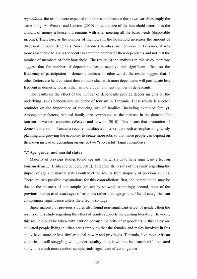
45

dependants, the results were expected to be the same because these two variables imply the

same thing. As Weaver and Lawton (2010) note, the size of the household determines the

amount of money a household remains with after meeting all the basic needs (disposable

income). Therefore, as the number of members in the household increases the amount of

disposable income decreases. Since extended families are common in Tanzania, it was

more reasonable to ask respondents to state the number of their dependants and not just the

number of members of their household. The results of the analyses in this study therefore

suggest that the number of dependants has a negative and significant effect on the

frequency of participation in domestic tourism. In other words, the results suggest that if

other factors are held constant then an individual with more dependants will participate less

frequent in domestic tourism than an individual with less number of dependants.

The results on the effect of the number of dependants provide deeper insights on the

underlying issues beneath low incidence of tourism in Tanzania. These results is another

reminder on the importance of reducing size of families (including extended family).

Among other factors, reduced family size contributed to the increase in the demand for

tourism in western countries (Weaver and Lawton, 2010). This means that promotion of

domestic tourism in Tanzania require multifaceted intervention such as emphasizing family

planning and growing the economy to create more jobs so that more people can depend on

their own instead of depending on one or two “successful” family member(s).

7.7 Age, gender and marital status

Majority of previous studies found age and marital status to have significant effect on

tourism demand (Brida and Scuderi, 2013). Therefore the results of this study regarding the

impact of age and marital status contradict the results from majority of previous studies.

There are two possible explanations for this contradiction: first, the contradiction may be

due to the biasness of our sample (caused by snowball sampling); second, most of the

previous studies used exact ages of responds rather than age groups. Use of categories can

compromise significance unless the effect is so huge.

Since majority of previous studies also found non-significant effect of gender, then the

results of this study regarding the effect of gender supports the existing literature. However,

this result should be taken with caution because majority of respondents in this study are

educated people living in urban areas implying that the females and males involved in this

study have more or less similar social power and privileges. Tanzania, like most African

countries, is still struggling with gender equality; thus, it will not be a surprise if a repeated

study on a much more random sample finds significant effect of gender.

46

CHAPTER 8

IMPLICATIONS AND CONCLUSION

8.1 Implications

The results of this study provide both theoretical and practical implications. Theoretical

implications mainly point out theoretical (and methodological) issues that worth further

research. Practical implications focus on the important lessons relevant for tourism

business managers and policy makers eager to promote domestic tourism in Tanzania.

8.1.1 Theoretical implications The hypotheses of this study were formulated based on literature review. Some of the

hypotheses were supported and others not; since the present study is mainly exploratory

rather than confirmatory, the unsupported hypotheses do not necessarily mean that the

findings of the previous studies that guided formulation of those hypotheses were wrong in

the first place. Nevertheless, the fact that this study was conducted in a context different

from where much of the empirical evidence in the literature come from, cannot be ignored.

Besides, the present study is potentially a victim of biasness due to the snowball sampling

approach. Therefore, even if the results of the analyses suggest for example, awareness and

price perception do not have significant effect on participation in domestic tourism that

may not necessarily be true for the entire population of Tanzania. There is a need to test

these theories much more thorough by using a more randomly selected sample in order to

provide answers that are generalizable and robust enough for theory development.

8.1.2 Business implications There are a number of lessons for tourism business managers to learn from this study.

First, although the attitude towards domestic tourism of individuals surveyed in this study

is fairly high (average score 3.46) there is a room for more improvement (maximum

possible score is 5). The improvement of attitudes is possible because psychology studies

have indicated that attitudes are acquired (Simonson and Maushak, 2001; Hoyer et al.

2013) and they can be changed fairly predictably (Zimbardo & Leippe, 1991). One of the

ways to change people´s attitudes is through marketing communication. Marketing

communication, for example through ads, could have incredible results on changing

people´s attitude (Hoyer et al. 2013); of course, as long as the ads are well crafted. The

increasing use of mobile technology also offers enormous opportunity to communicate

tourism products to the local people. According to the Tanzania Telecommunication

47

Authority (TCRA), by December 2013 Tanzania had 27 million mobile phone

subscriptions; therefore as smart phones are becoming cheaper this means there is a great

opportunity to promote tourism products through social media platforms such as Facebook,

Youtube, and Twitter. Currently social media has attracted many users in Tanzania, and

this is an opportunity for tourism businesses to promote their products.

The second lesson is on the importance of market segmentation. The findings of this

study, just like previous studies, suggest that income has a huge impact on participation in

domestic tourism. That is, as income increase and so does participation in domestic

tourism. Important lesson is that tourism businesses should try to innovate cheaper

offerings in order to attract even people with lower incomes. For example group tours are

not so popular in Tanzania but it could one of the ways to lower costs per tourist, which in

turn can make it possible for people with lower incomes to participate in domestic tourism.

Market segments such as college students can be served pretty well through group tours.

More so, service providers such as restaurants and hotels at tourist destinations should try

to develop cheaper options and locally appealing products; you cannot design offerings by

with international tourists in your mind and yet go around complaining about the low turn

up of the local people.

8.1.3 Policy implications The government of Tanzania has lately been keen on promoting domestic tourism.

Initiatives such as public campaigns have been staged. The results of this study offer

important inputs to advance those initiatives. Short term and long term measures need to be

taken in order to promote growth of domestic tourism. The first short term measure is

continuing with campaigns for improving people´s attitudes towards domestic tourism.

Second, they should find ways to lower taxes on the tourism services sold to local people;

this will make prices relatively lower which in turn can allow even people with lower

income to participate in domestic tourism. However, to show more seriousness about this

matter they should embark on long term measures as well; for example since number of

dependants seem to affect participation in domestic tourism due to constrained disposable

income, then campaigns for family planning and creation of employment opportunities are

likely to improve domestic tourism in the future. And to tell the truth (surely bitter one) the

real solution for improving domestic tourism in Tanzania is to fight poverty. It is absurd

that the government is dreaming to increase domestic tourism in a country where majority

of people live below the absolute poverty line. General increase in wealth is associated with

participation in domestic tourism (Weaver and Lawton, 2010).

48

8.2 Conclusion and limitations of the study

The present study aimed at exploring the relationship between social economic factors

and participation in domestic tourism in Tanzania. The social economic factors under study

were: income level, level of awareness about domestic tourism, attitude towards domestic

tourism, number of dependants and the level of perceived price. These factors were

selected based on findings of the previous studies. The objective of the study was achieved

through collection and quantitative analysis of empirical data.

In response to the first research question, the results of the analysis have shown that,

among the social-economic factors identified, participation in domestic tourism in Tanzania

is significantly related to: income level, attitudes towards domestic tourism and number of

dependants. Contrary to the hypotheses, the results have shown that the level of awareness

and perception of relative prices do not have significant effect on participation in domestic

tourism. Likewise, the control variables age, marital status and gender did not have

significant effect. The second question addressed in this study is regarding the moderation

effect of other social economic factors on the relationship between attitude and

participation in domestic tourism in Tanzania. Among the social-economic factors income

was selected for the moderation test because based on the findings of the previous studies,

it is the most influential factor determining tourism demand. The results of the moderation

test indicate that although attitude is a significant predictor of participation in domestic

tourism, its effect depends on the income level.

Various implications have been asserted in connection to the results of the analyses

conducted in this study. The insights revealed through the analyses provide guidance to the

tourism business managers and policy maker who are committed to develop domestic

tourism in Tanzania. However, it is important to note the results of this study should not be

regarded as confirmatory due to the potential biasness of the sample used. This study

applied snowball-sampling technique whose main weakness is the likelihood of giving a

sample of individuals with similar characteristics. Such a sample is apparently associated

with high risk of biasness, and this is the main limitation of this study. Therefore, one of

the potential areas for further research could be conducting a similar study by collecting

data from a much more random sample and perhaps including other social-economic

variables in the multivariate model.

.

49

References

Aaker, D.A. et al., 2011. Marketing Research 10th ed., Singapore: John Wiley & Sons

(Asia) Pte Ltd.

Ajzen, I. (1988). Attitudes, personality, and behavior. Chicago: Dorsey.

Alegre, J., and Pou, L. (2004). Micro-economic determinants of the probability of tourism

consumption. Tourism Economics, 10(2), 125-144.

Alegre, J., Mateo, S., and Pou, L. (2009). Participation in tourism consumption and the

intensity of participation: an analysis of their socio-demographic and economic

determinants. Tourism Economics, 15(3), 531-546.

Alegre, J., Mateo, S., and Pou, L. (2010). An analysis of households’ appraisal of their

budget constraints for potential participation in tourism. Tourism Management, 3145-

3156.

Alegre, J., Mateo, S., and Pou, L. (2013). Tourism participation and expenditure by

Spanish households: The effects of the economic crisis and unemployment. Tourism

Management, 39, 37–49.

Altinay, L., and Paraskevas, A. (2008). Planning research in hospitality and tourism.

Burlington: Elsevier : Butterworth-Heinemann.

Bank of Tanzania (2010). Tourism Sector Survey. International Visitors’ Exit Survey

Report. available at: http://www.bot-tz.org/Publications/TTSS/2008_Survey.pdf

Bishop, George F., Robert W. Oldendick, Alfred J. Tuchfarber, and Stephen E. Bennett,

(1980), "Pseudo-Opinions on Public Affairs." Public Opinion Quarterly. 44(2):198-209.

Boo, S., Busser, J., & Baloglu, S. (2009). A model of customer-based brand equity and its

application to multiple destinations. Tourism Management, 30, 219–231.

Brida, J. G., & Scuderi, R. (2013). Determinants of tourist expenditure: A review of

microeconometric models. Tourism Management Perspectives.

Bryman, A. & Cramer, D., (2009). Quantitative Data Analysis with SPSS 14,15 & 16: A

Guide for Social Scientists, London: Routledge.

Burns, Robert & Burns, Richard, 2008. Business Research Methods and Statistics Using

SPSS, London: Sage Publications Ltd.

Cai, L. A. (1998). Analyzing household food expenditure patterns on trips and vacations: a

tobit model. Journal of Hospitality and Tourism Research. 22(4): 338-358.

Chiu, L.K. and K. Kayat, 2010. Psychological determinants of leisure time physical activity

participation among public university students in malaysia. AJTLHE, 2(2): 33-45.

50

Duerden, M. D., and Witt, P. A. (2010). The impact of direct and indirect experiences on the development of environmental knowledge, attitudes, and behaviour. Journal of Environmental Psychology, 30(4): 379-392.

Easterby-Smith, M.; Thorpe, R.; Lowe, A. (2002) Management Research, 2nd ed. London: SAGE Publications.

Field, A (2013). Discovering Statistics Using IBM SPSS STATISTICS. 4th ed. London: SAGE Publications.

Hagemann, R. P. (1981). The determinants of household vacation travel: some empirical evidence. Applied Economics, 13(2): 225-234.

Hoyer, W.D., MacInnis, D. and Pieters, R. (2013). Consumer Behavior, 6th Edition. (South-Western: Cengage learning).

Iacobucci, D. & Churchill, G.A., (2010). Marketing Research Methodological Foundations International Edition 10th ed., Hampshire: South-Western Cengage Learning.

Kim, S. S., Prideaux, B., & Chon, K. (2010). A comparison of results of three statistical methods to understand the determinants of festival participants' expenditures. International Journal of Hospitality Management, 29(2), 297–307.

Kladou, S., & Kehagias, J. (2014). Assessing destination brand equity: An integrated approach. Journal of Destination Marketing and Management, 3, 2–10.

Kline, P. (1999). The handbook of psychological testing (2nd ed). London: Routledge. Kraus, S. J. (1995). Attitudes and the prediction of behavior: A meta- analysis of the

empirical literature. Personality and Social Psychology Bulletin, 21, 58–75. Kumar, Ranjit, 2005, Research Methodology-A Step-by-Step Guide forBeginners,

(2nd.ed), Singapore, Pearson Education. Lee, R.M. (1993) Doing Research on Sensitive Topic. London: Sage. Lim, C., (2006), A survey of tourism demand modeling practice: Issues and implications.

In International Handbook on the Economics of Tourism, ed. By l. Dwyer, and P. Forsyth, Northampton, Edward Elgar Publishing, pp. 45-72.

Maina, N. (2006). Desire for electronic entertainment in Africa. Available at: http://www.bizcommunity.com/Article/111/66/12397.html

Mariki, S. B1., Hassan, S. N., Maganga, S. L. S., Modest, R. B. and Salehe, F. S. (2011). Wildelife-based Domestic Tourism in tanzania: Experiences from Northern Tanzania. Ethiopian Journal of Environmental Studies and Management. 4 (4): 62 - 73.

Melenberg, B., & Van Soest, A. (1996). Parametric and semi-parametric modelling of vacation expenditures. Journal of Applied Econometrics, 11, 59-76.

Mergoupis, & Steuer, M. (2003). Holiday taking and income. Applied Economics, 35(3), 269-284.

Minnaert, L. (2014). Social tourism participation: The role of tourism inexperience and uncertainty. Tourism Management, 40, 282–289.

Mutinda, R. and Mayaka, M. (2012). Application of destination choice model: Factors influencing domestic tourists destination choice among residents of Nairobi, Kenya, Tourism Management. 33(6): 1593 - 1597.

Neuman, W.L. (2005) Social Research Methods (6th edn). London: Pearson. Nicolau, J. L., & Mas, F. (2005). Heckit modeling of tourist expenditure: evidence from

Spain. International Journal of Service Industry Management, 16(3), 271e-93.

51

Nicolau, J. L., & Mas, F. (2009). Simultaneous analysis of whether and how long to go on

holidays. The Service Industries Journal, 29(8): 1077-1092.

Nunnally, J. C. (1978). Psychometric theory (2nd ed.). New York: McGraw-Hill.

Pierrret, F. (2011).Some Points on Domestic Tourism. An adaptation of a lecture delivered

during the « Rencontre internationale sur le développement du tourisme domestique »

Algiers, 9 Dec. 2010. Available at: http://www2.unwto.org/en/agora/some-points-

domestic-tourism

Ragheb, M., & Beard, J. (1982). Measuring leisure attitude. Journal of Leisure Research, 5,

155-167.

Ragheb, M.G., & Griffith, C.A. (1982). The contribution of leisure participation and leisure

satisfaction to life satisfaction of older persons. Journal of Leisure Research 14: 295-

306.

Ragheb, M.G., & Tate, R.L. 1993. A behaviour model of leisure participation based on

leisure attitude, motivation and satisfaction. Leisure Studies 12: 61-71.

Saunders, M., Lewis P., and Thornhill, A. (2012).Research Methods for Business Students (6th

edition). Edinburgh: Pearson Education Limited.

Sherman, S. J., & Fazio, R. H. (1983). Parallels between attitudes and traits as predictors of

behavior. Journal of Personality, 51, 308–345.

Sindiga, I. (1996). Domestic Tourism in Kenya. Annals of Tourism Research. 23(1):19-31.

Stevens, J. (2002). Applied Multivariate Statistics for the Social Sciences (4th Edition). Mahwah,

NJ: Lawrence Erlbaum Associates.

Stevens, S.S., 1946. On the Theory of Scales of Measurement. Science, New Series, 103(2684):

677–80.

Sudman, Seymour and Norman M. Bradburn, "Questions for Measuring Knowledge," Chapter 4 (pp 88-118) in Asking Questions. Jossey-Bass: San Francisco, 1982.

Taylor, T., & Arigoni, O. R. (2009). Impacts of climate change on domestic tourism in the UK: a panel data estimation. Tourism Economics, 15(4), 803-812.

Van Soest, A., & Kooreman, P. (1987). A micro-economic analysis of vacation behaviour. Journal of Applied Econometrics. 2: 215-226.

Weaver, D., and Lawton, L. (2010). Tourism Management. 4th edition. Wiley Australia. Wen, Z. (1997). China’s domestic tourism: impetus, development and trends. Tourism

Management, 18, 565-571. Wu, L., Zhang, J., & Chikaraishi, M. (2012). Representing the influence of multiple social

interactions on monthly tourism participation behavior. Tourism Management. Yan, T., Curtin, R., and Jans, M. (2010). Trends in Income Nonresponse Over Two

Decades.Journal of Official Statistics, 26, (1), 145-164. Zimbardo, P. & Leippe, M. (1991). The psychology of attitude change and social influence.

Philadelphia, PA: Temple University Press.

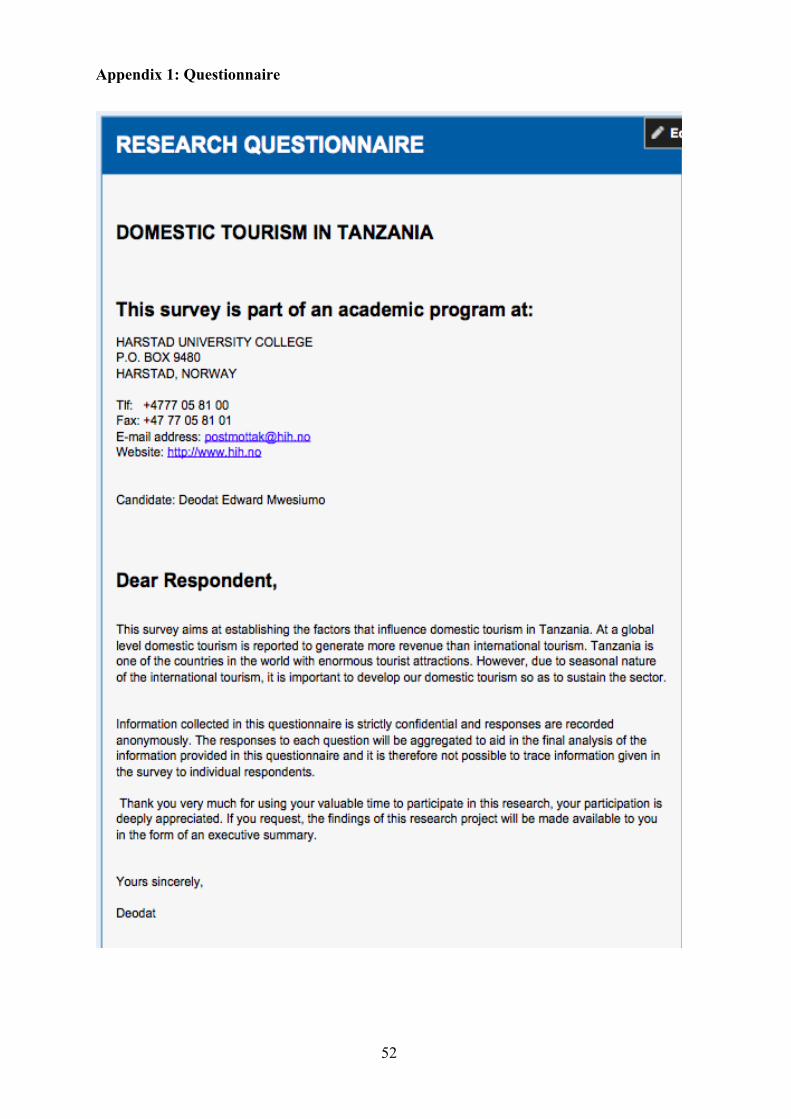
52

Appendix 1: Questionnaire

53

54

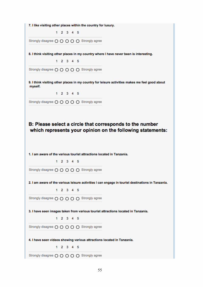
55

56

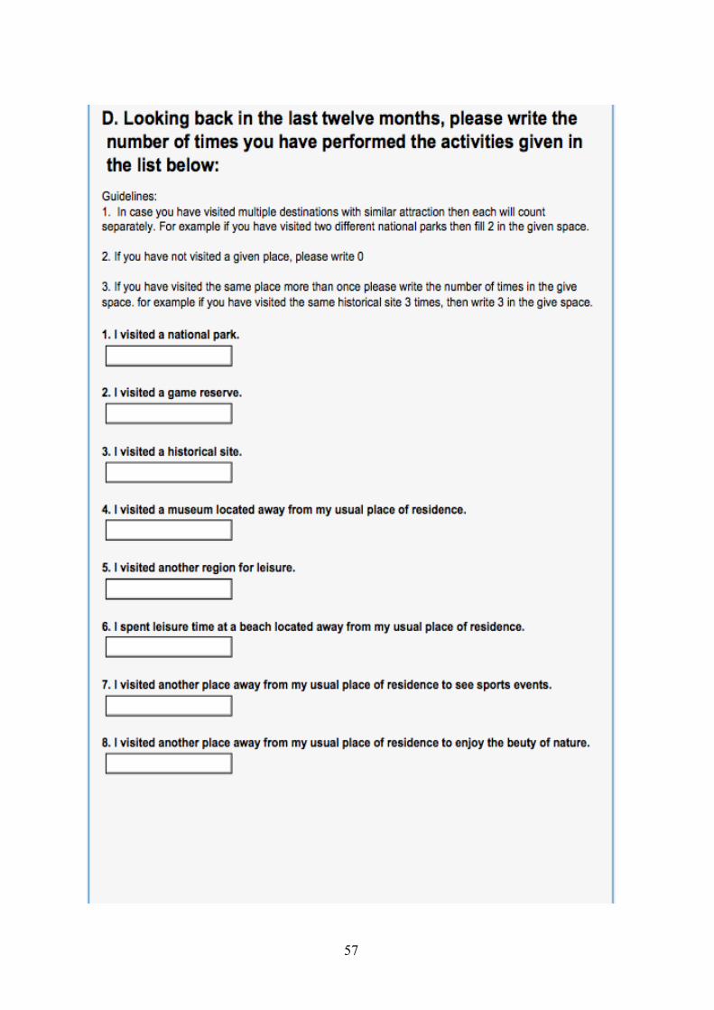
57

58

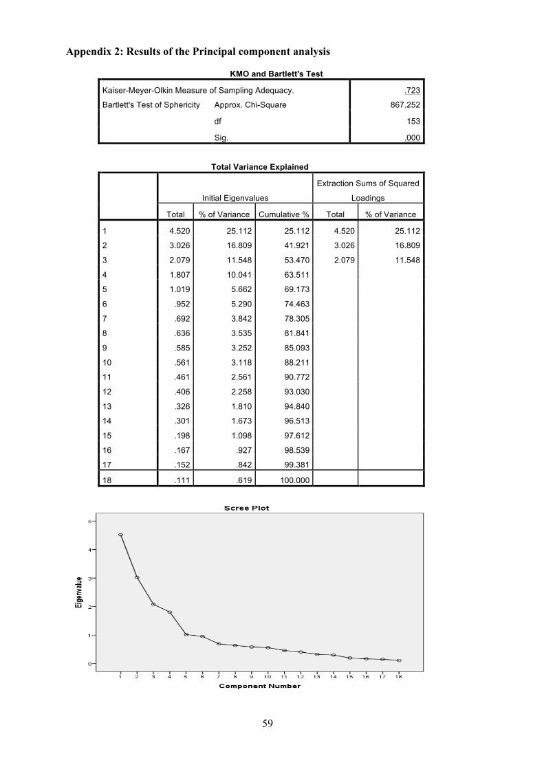
59

Appendix 2: Results of the Principal component analysis

KMO and Bartlett's Test

Kaiser-Meyer-Olkin Measure of Sampling Adequacy. .723

Bartlett's Test of Sphericity Approx. Chi-Square 867.252

df 153

Sig. .000

Total Variance Explained

Initial Eigenvalues

Extraction Sums of Squared

Loadings

Total % of Variance Cumulative % Total % of Variance

1 4.520 25.112 25.112 4.520 25.112

2 3.026 16.809 41.921 3.026 16.809

3 2.079 11.548 53.470 2.079 11.548

4 1.807 10.041 63.511 5 1.019 5.662 69.173 6 .952 5.290 74.463 7 .692 3.842 78.305 8 .636 3.535 81.841 9 .585 3.252 85.093 10 .561 3.118 88.211 11 .461 2.561 90.772 12 .406 2.258 93.030 13 .326 1.810 94.840 14 .301 1.673 96.513 15 .198 1.098 97.612 16 .167 .927 98.539 17 .152 .842 99.381 18 .111 .619 100.000

60

Appendix 3: Visual assessment of Skewness

61

Appendix 4: Tests for assumptions of regression analysis

(a) Linearity and heteroscedasticity

(b) Multicolinearity

Tolerance VIF

ATTIT 0.154 1.202

PRICE_PERC -0.009 2.187

DEPS -0.393 1.121

AWAR -0.016 1.073

D_INC1 0.235 1.707

D_INC2 0.379 2.878

AVERAGE = 1.7

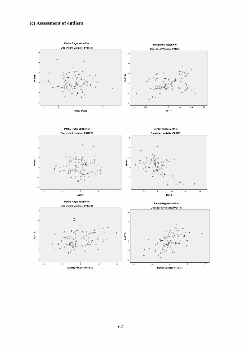
62

(c) Assessment of outliers

63

Appendix 5: Post hoc test for comparing participation across incomes

(a) Descriptives

N Mean

Std. Deviation

Std. Error

95% Confidence Interval for Mean

Minimum Maximum Lower Bound

Upper Bound

Below Tzs. 1000000 38 2.87 1.647 0.267 2.33 3.41 0 7

Tzs. 1000000 - 3000000 33 3.85 1.716 0.299 3.24 4.46 0 7

Above Tzs. 3000000 32 5.50 2.125 0.376 4.73 6.27 0 8

Total 103 4.00 2.114 0.208 3.59 4.41 0 8

(b) Test of Homogeneity of Variances

PARTICIPATION Levene Statistic df1 df2 Sig.

1.380 2 100 0.256

(c) Post hoc test: Tukey HSD

(I) INCOMECAT Income category

(J) INCOMECAT Income category

Mean Difference

(I-J) Std.

Error Sig.

95% Confidence Interval

Lower Bound

Upper Bound

Tukey HSD

Below Tzs. 1000000 Tzs.1000000 - 3000000 -0.980 0.435 0.068 -2.02 0.06

Above Tzs. 3000000 -2.632* 0.439 0.000 -3.68 -1.59

Tzs.1000000 - 3000000

Below Tzs. 1000000 0.980 0.435 0.068 -0.06 2.02

Above Tzs. 3000000 -1.652* 0.454 0.001 -2.73 -0.57

Above Tzs. 3000000 Below Tzs. 1000000 2.632* 0.439 0.000 1.59 3.68

Tzs.1000000 - 3000000 1.652* 0.454 0.001 0.57 2.73

*. The mean difference is significant at the 0.05 level.

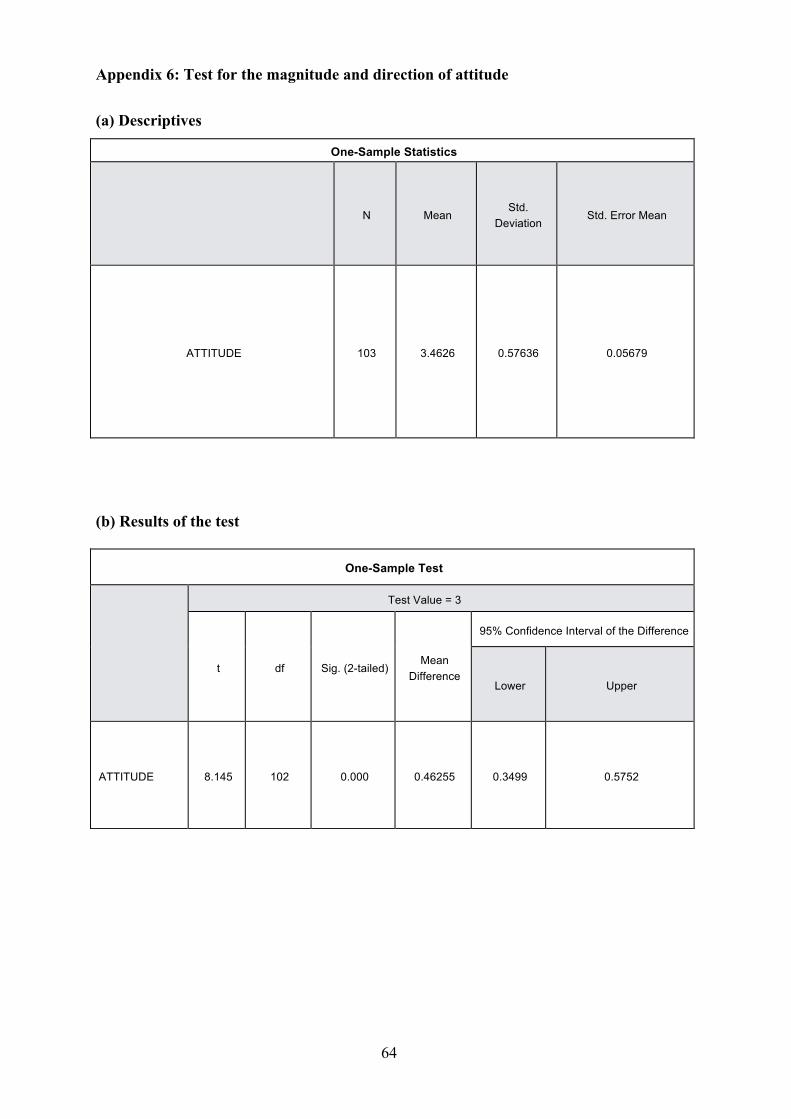
64

Appendix 6: Test for the magnitude and direction of attitude

(a) Descriptives

One-Sample Statistics

N Mean Std. Deviation Std. Error Mean

ATTITUDE 103 3.4626 0.57636 0.05679

(b) Results of the test

One-Sample Test

Test Value = 3

t df Sig. (2-tailed) Mean Difference

95% Confidence Interval of the Difference

Lower Upper

ATTITUDE 8.145 102 0.000 0.46255 0.3499 0.5752

65

Appendix 7: Test for the magnitude and direction of awareness

(a) Descriptives

One-Sample Statistics

N Mean Std. Deviation Std. Error Mean

AWARENESS 103 3.42 0.590 0.058

(b) Results of the test

One-Sample Test

Test Value = 3

t df Sig. (2-tailed)

Mean Difference

95% Confidence Interval of the Difference

Lower Upper

AWARENESS 7.228 102 0.000 0.420 0.30 0.54

66

Appendix 8: Test for the magnitude and direction of price perception

(a) Descriptives

One-Sample Statistics

N Mean Std. Deviation Std. Error Mean

PRICE_PERCEPTION 103 3.14 1.154 0.114

(b) Results of the test

One-Sample Test

Test Value = 3

t df Sig. (2-tailed)

Mean Difference

95% Confidence Interval of the Difference

Lower Upper

PRICE_PERCEPTION 1.224 102 0.224 0.139 -0.09 0.36