AD-A234 123RL-TR-91 -6In-House ReportFebruary 1991

DIGITAL LOGIC TESTING ANDTESTABILITY

Warren H. Debany, Jr.

APPROVED FOR PUBLIC RELEASE DISTRIBUTION UNLIMITED

DTIGPRl 0 4 mill

Rome LaboratoryAir Force Systems Command

Griffiss Air Force Base, NY 13441-5700

This report has been reviewed by the Rome Laboratory Public Affairs Office(PA) and is releasable- to the National Technical Information Service (NTIS). At NTISit wilt be releasable to the general public, including foreign nations.

RL-TR -91-6 has been reviewed and is approved for publication.

APPROVED:

EDGAR A. DOYLE, r ,Atting ChiefMicroelectronics Reliability DivisionDirectorate of Reliability and Compatibility

APPROVED:

JOHN J. BART, Technical DirectorDirectorate of Reliability and Compatibility

FOR THE COMMANDER:

RONALD RAPOSODirectorate of Plans and Programs

If your address has changed or if you wish to be removed from the RL mailing list, orif the addressee is no longer employed by your organization, please notify RL(RBRA)Griffiss AFB, NY 13441-5700. This will assist us in maintaining a current mailing list.

Do not return copies of this report unless contractual obligations or notices on a,erific document require that it e returned.

REPORT DOCUMENTATION PAGE OnMBE R0v08

ME No 62 070-08

purgo mn us foo t. l ogW* =l= o, wldc ph w- ww ftobctag n o tp =m SendIk c rnw f rag ,dngd~ ba =aaorV a 0 gan w d~ "or

oao, l Run w o= n:k * w-gno for raduris ad. R Ito Wea*Vo Hewqw SavticM M fcoo fomtcmrNn Opw a-Repar 5 dJe

De/a .Hiqw" . Sft 1204. A*bo VA 22202P4=1 "r: tn " Ofe i MrogRwel w-i Budgmt P pwwk Redcto Propel (WO&M ,,0U Woo*Vt OC 25

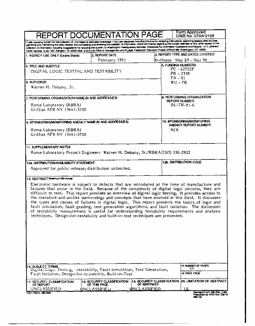
1. AGENCY USE ONLY (Leave Blank) 2 REPORT DATE a3 REPORT TYPE AND DATES COVERED

February 1991 Iln-House May 89 - Nov 90

4. TITLE AND SUBTITLE 5, FUNDING NUMBERS

DIGITAL LOGIC TESTING AND TESTABILITY PE - 62702FPR - 2338TA - 01

, AUTHOR(S) WU - 7BWarren H. Debany, Jr.

7. PERFORMING ORGANIZATION NAME(S) AND ADDRESS(ES) 8. PERFORMING ORGANIZATIONREPORT NUMBER

Rome Laboratory (RBRA) RL-TR-91-6Griffiss AFB NY 13441-5700

9. SPONSORINGIMONITORING AGENCY NAME(S) AND ADDRESS(ES) 10. SPONSORING/MONITORINGAGENCY REPORT NUMBER

Rome Laboratory (RBRA) N/AGriffiss AFB NY 13441-5700

11. SUPPLEMENTARY NOTESRome Laboratory Project Engineer: Warren H. Debany, Jr./RBRA/(315) 330-2922

1 U. DSTRIBUTION/AVAILABIUTY STATEMENT 1 2. DISTRIBUION CODE

Approved for public release; distribution unlimited.

13, ABTRACT~m"2 mw

Electronic hardware is subject to defects that are introduced at the time of manufacture andfailures that occur in the field. Because of the complexity of digital logic circuits, they aredifficult to test. This report provides an overview of digital logic testing. It provides access tothe literature and unifies terminology and concepts that have evolved in this field. It discussesthe types and causes of failures in digital logic. This report presents the topics of logic andfault simulation, fault grading, test generation algorithms, and fault isolation. The discussionof testability measurement is useful for understanding testability requirements and analysistechniques. Design-for-testability and built-in-test techniques are presented.

14. SUB.JECT TERMS ,, NI ,TR OF PAGESDi6itai Lo6. Testig, I estability, Fault Simulation, Test Generation,Fault Isolation, Design-for-tc3tability, Built-in-Test I a PRICE coDE

17. SECURVIr CLASSIFICATiON 18, SECURITY CLASSIFICATION 19. SECURITY CLASSIFICATION 20. UMITATION OF ABSTRACTOF REPORT OF THIS PAGE OF ABSTRACT

UNCLASSIFIED JNCLASSIFIEu NCLASSIFIED ULNSN 7S4"0 -29a4=~ Pruto vim FNS 296Z.P -lK I9/nANSl 9:ZAAt

29&1132

Table of Contents

Section Page No.

1 Introduction 1

2 Basic Principles 321 Failures, Faults, Errors, and Testing 4

2.2 Fault Models 6

2.3 Multiple Faults 8

2.4 Non-Stuck-At Failures 9

3 Tools for Grading Tests 13

3.1 Fault Coverage vs. Field Rejects 13

3.2 Logic Simulation Mechanisms 15

3.3 Fault Simulation Mechanisms 16

3.4 Variability of Results 20

4 Tools for Generating Tests 23

4.1 Computational Difficulty 23

4.2 Combinational Logic Testing 24

4.3 Sequential Logic Testing 28

4.4 Memory Testing 29

5 Fault Isolation Techniques 33

5.1 Adaptive Fault Isolation Techniques 33

5.2 Preset Fault Isolation Techniques 355.3 Cost and Accuracy of Fault Isolation 35

6 Testability Measurement 37

6.1 Testability Measures and Factors 37

6.2 Tools for Testability Measurement 387 Design-For-Testability and Built-In-Test 41 on For

7.1 Design-for-Testability 42 GRA&"AB 0l

7.2 Built-In-Self-Test 43 ,unced 57.3 Built-In-Self-Check 45 '"catlon

8 Conclusions 47References 49 7-.-------

a' Allability CodesDi~ Avail and/or

'61st [Speolal

I Introduction

This report addresses the problem of testing digital logic circuits. It has been written with

the goal of providing a survey of the current state-of-the-art and supplying the interested

novice reader with access to the relevant literature. The writing of this report stemmed

from a request by Dr. Mel Cutler of Aerospace Corporation for an introductory piece for a

chapter of a book in a morograph series, and his help is gratefully acknowledged. Because

of changes in editorships and questions about the eventual classification of the monograph

series, this overview section was withdrawn from consideration in the monograph and was

expanded into its current torm. The scope of this report is more narrow than the title might

promise, unfortunately, because its original direction was oriented toward aspects of testing

and testability as they applied to digital signal processing hiidware.

This report contains an overview of digital testing, and is intended to provide "starter"

knowledge. Initial access to a field of knowledge is often difficult for a researcher to obtain.

The primary reason for this is that it is a laborious task to research a field. To some degree

this task is becoming less onerous with the availability of on-line data base search capabilities,

but the scope of these searches is generally limited to the keywords jotted down by authors

at the last moment before submitting a paper, or is limited to small text fragments such as

abstracts. There is no substitute for a decade or so of concentrated effort in collecting the

desired information through references, personal contacts, and serendipitous finds.

The references cited in this report represent only a small fraction of the Literature that

is applicable to even the small part of the topic that is addressed here. In order to keep the

size of the report manageable it was necessary to omit many excellent references. In general,

no more than two references are given when possible. The first reference is a seminal one

that introduces !he topic. The second reference is a more recent or more readily available

one that provides both more up-to-date information and, in its own citations, a detailed

chronology of the specific area.

A second reason that it is difficult for a researcher to get started in a new field is that every

field of knowledge evolves rapidly into a tangle of confusing, contradictory, and anachronistic

terms and definitions. This report attempts to provide cross references among terms in

the digital testing area. This has been done with awareness that, in the effort to unifiy

terminology, some new terminology has been introduced.

1

2 Basin Principles

Modern control, communications, computing, and signal processing systems rely heavily on

the use of digital electronic circuits. Systems based on digital logic such as microprocessors

and specialized controllers, with large amounts of memory, perform sophisticated algorithms

at high speed, and because of reprogrammability can be highly adaptable. Even fixed func-

tions, such as FFT processors, use components such as floating-point multipliers, adders, and

registers. Electronic hardware is used in mission-critical and even flight-critical functions.

However, electronic hardware, including digital logic, is subject to defects or failures that

occur both at the manufacturing level and in the field. Because erroneous output may not

occur immediately, 't is not always apparent that a failure has occurred.

Fault-tolerant design techniques can compensate for mauy expected failure types that

occur during system operation, but in order to be able to take appropriate action in the

event of a failure it must be known that a failure has occurred and, generally, where the

failure is located. Thus, a necessary step in building a fault-tolerant system is to provide

fault detection and fault iso1ti--n capability.

Analytical .and probnbilistic models for fault-tolerant designs are used to determine their

efTectiveness, required spares overhead, impact on performance, possible degraded modes

of operation, and single-point failures. The models are, almost without exception, based

on an assumption that is seldom stated explicitly: that the hardware initially contains no

defects. This means that all manufacturing defects are assumed to have been eliminated

frotn all subassemblies down to and including the integrated circuits (ICs) and associated

interconnect.

This report discusses some of the causes and effects of digital logic failures. The goal is

to present the reader .-.th enough information so as to gain effective access to the relevant

literature. The discussion is limited to hardware failures experienced by IC-based systems;

although design errors in hardware and software are known to be significant causes of system

failure they will not be discussed in this report. It is shown that, in general, test generation

is a comp.'tationally difficult problem. This report discusses what can be done to improve

the testability of digital logic and the tools and techniques that are available.

3

2.1 Failures, Faults, Errors, and Testing

General terminology has been established for fault-tolerant computing applications [Aviz82]

[Aviz86). Definitions for "failure," "fault," and "error" have been described in abstract terms

that are applicable from the component to the system level. In this report it is necessary

to narrow the definitions of these and related terms so that they apply consistently and

specifically to the problem of diagnosing defects in digital electronic equipment. The terms

used ;n this report are based on work by Aviienis [Aviz82] and Aviiienis and Laprie [Aviz86]

and are used specifically in accordance with Timoc, et al. [Tim83], and Abraham and Fuchs

~Abre9J.

A failure is considered to be the actual defect that is present in hardware. It is ass-!med

that incorrect behavior always hsm a struttural basis, that is, it is always due to a physica!

influence or a physical defect. This does not exclude incorrect behavior caused by an out-of-

specification component, such as a transistor with low gain, or a probabilistic process. such

ts 1 it error rate governed by a signal-to-noist ratio.

,Vanufactu1ing-level failures are those that are introduced at the time of manufacture

andor assembly. Other defects occur during operation or storage after the hardware has

been deployed; these are said to be field failures, field-level failures, or operational failurcs.

General failure types for ICs have been categorized and include opens, shorts or bridging,

and changes iO circuit characteristics (Abra861 rChand87i [Levi81] [Maly871 [Shen85] [Siew821ririF31 'Wad78hl. Cause-. of IC failure at the manufacturing level include photolithogra-

phy errors, ,cntarninai, and poor process control. In the field, IC failure mechanisms

irclude electroinigration, electrostatic discharge, hot-electrons, and effects 'aused by radia-

tion Many technmques can be used to improve IC producibility and reliability such as the

une of conservative circuit design rules and input protection circuits. Above the IC level,

assemblies iiuCh as printed circuit boards primarily experience opens and shorts in their in-

terconnect. and failures in discrete components such as resistors, capacitors, switches, relays,

etc

,, fault is aii abstraction or idealization of a failure; it is a logical model of a failure's

erpected bolkavior 'layes85: TiM831. The most commonly-used is the stuck-at-zero (SAC)

and ituck-at-one (.5 1) fault model, or simply the stuck-at fault model. In the stuck-at

mode!, the Irzi, gates are assumed to be fault-free, and the effect of any failure is assumed

o be ,-quivalet to having a constant logic zero or logic one present on a logic signal line. For

4

example, an open (e.g., broken or missing) signal line in an IC implemented in Low-Power

Schottky technology exhibits SA1 behavior because of the leakage current supplied by the

input of any logic gate connected to the logic line after the site of the open.

Because the meaning will be clear in context, the term "faulty" is used when referring

either to the actual item that contains a failure or to the model of the item that contains a

fault. The term "fault-free" is used when referring either to an item that does not contain a

failure or to the model of the item that does not contain a fault.

An error is an observable difference between the outputs of a fault-flee and faulty item-

under-test. The item-under-test can be an IC, board, module, or system. The occurrence

of a failure does not necessarily result in an immediate occurrence of a eiror. The "time"

between the occurrence of a failure to the first occurrence of an error is called the error

latency. "Time" may be measured in terms of wall-clock time, number of clock cycles, or

number of test vectors.

Testing is the process of applying a sequence of input values to an item and observing

output values, with the goal of causing any of a given set of failures, that can potentially

exist in the item, to exhibit an error. An undetectable failure is one for which no possible

test can cause an errcr to be observed. An undetected failure, with respect to a given test,

is one that can cause an error under some set of conditions but does not cause an error in

response to the given test.

In this report a test is a sequence of one or more test steps, where each test step corre-

sponds to a sequence of one or more test vectors.' This hierarchy of terms follows the natural

hierarchy of test development. For example, in testing a random-access memory (RAM):

" A complete Walking Ones and Zeros pattern [Breu76] is a single test.

" A Walking Ones and Zeros test consists of many test steps that each involve writing

to, or reading from, memory locations.

* Each test step that writes to a memory location consists of several test vectors that in

sequence: enable the memory, set an address, apply data, and strobe the write enable.

This report is concerned with manufacturing-level and field-level testing of digital logic

to detect and isolate failures. However, design errors can also be considered to be failures.

Testing for design errors is more generally referred to as verification testing or design veri-

A test vector represents a single stimulus/response test cycle (perhaps conditioned by timing information)

or the automatic test equipment.

5

fication. Testing for misinterpretation of requirements is called validation testing or design

validation. Verification and validation testing are not discussed in this report.

2.2 Fault Models

The correspondence between failures and faults is the subject of debate. Most practical

tools for test generation or test grading rely not only on using the stuck-at fault model, but,

furthermore, assume that the faults are single and permanent as well. That is, it is assumed

that any failure that occurs can be adequately modeled by a SAO or a SAl value on exactly

one logic line. For brevity, we refer to the fault model consisting of "single, permanent, SAO

and SAt fnults on the logic lines" as the single-stuck-line (SSL) iHayes85] fault model. We

refer to the fault model consisting of "multiple, permanent, SAO and SAl faults on the logic

lines" as the multzple-stuck-line (MSL) fault model.

There is no question that the SSL fault model is inadequate for modeling failures in

.'lnury iCs; for that reason, test generation [Aba831 and test grading '50121 for memories

.s t.:,lie using techniques and algorithms that specifically address memory structures. It

is well-known that the SSL fault model does not account for the behavior of all possible

failures in digital ICs [iHayes85] [Tim83] [Hart88] [Abra86] [Levi8i] [Siew78]. It is easy to

find counterexamples to the SSL model, such as fmaures that correspond to MSL faults, or

are not permanent, or affect characteristics such as circuit delays.

It is common to use a simple fault model even when a more complex fault model is known

,3 1-e more appropriate: in fact, this is a fundamental part of the concept of modelling. The

only problem is to decide how much detail should be traded for cost. Let Mi denote a simple

fault model and let M2 denote a more accurate yet far more complex fault model. It may

be aceptabie to use M1 instead of M2 if the following two conditions are met:

" the cost involved in considering M2 is prohibitive compared to that of considering M1,

and

* a test set that detects all or nearly all faults in M1 also detects all or nearly all faults

in W2.

In other words, if asing U1 costs far less, and produces substantially the same results as

using M2, then use MI1.

Consider the 54LS181 four-bit arithmetic logic unit (ALU) [T176). The 54LS181 has

14 primary inputs, 8 primary outputs, and no memory (i.e., contains no flip-flovs, latches,

6

or asynchronous combinational feedback paths). The 54LS181 logic model used in these

examples is composed of 112 logic gates. There are 126 distinct nodes, and 261 logic lines

in the 54LS181.' Using the SSL fault model, the 261 logic lines currespond to 522 stuck at

faults that must be considered for test grading or test generation. Sections 3 and 4 discuss

tools and techniques that are available for these purposes. The equivalent of 523 different

logic models for the 54LS181 (1 fault-free and 522 faulty) must be considered when the SSL

fault model is used. Because the number of SSL faults is proportional to the number of logic

lines, and the number of logic lines is approximately proportional to the number of gates,

the number of SSL faults in a logic model is approximately proportional to the number of

gates. In this example, there are 4.7 SSL faults per gate.

For a given logic model, let L be the number of lines, N be the number of nodes, r be the

multiplicity of a multiple fault (number of lines that are simultaneously SAO or SAI), and

s be the multiplicity of a single bridging fault (number of nodes that are shorted together).

Then the number of multiple faults of multiplicity m is given by 2m (.L) and the number of

single bridging faults' of multiplicity . is given by (N).

In contrast to the "simple" SSL fault model, in which the 54LS181 is considered to have

522 faults, the number of MSL faults of multiplicity 2 is 135,720 and the number of bridging

failures of multiplicity 2 is 7,875. Totaling the number of faults of multiplicity 2, 3, 4, and 5,

their are .3.14x10 1 SSL and MSL faults, and 2.55x10 s single and multiple bridging faults.

In sections 3 and 4 it is shown that it is not necessary to process a complete, distinct

logic model when considering a given fault. Instead, techniques have been developed that

simulate only the differences between fauic-iree and fr'ilt:' ,erqions of the item-under-test,

and, furthermore, do so for many or even all versions simultaneously. However, while the

number of faults considered when using the SSL nid grows approximately linearly with

the number of gates, the number grows exponentially in the cases of MSL faults or bridging

failures. Exponential growth means that, in practical terms, we cannot even list the set of

faults for items-under-test of even modest size, much less simulate their effects.

Tools are available that can operate effectively with the SSL fault model (or variations

thereof) but we wish to deal accurately with the more realistic fault models. Much of

the research involving the more realistic fault models has been concerned with determining

A set of connected logic lines constitutcs a nodc.

'Note that a single bridging fault is a single instance of shorted nodes, Many node may be involved.

7

under what conditions the SSL fault model is sufficient to give valid results, how to reduce

a problem to the complexity of SSL fault modelin,',, and how to analytically derive results

that do not rely on explicit enumeration of faulta.

Most of the current interest in technology-specific failures is in CMOS failure types, be-

cause CMOS is currently the dominant circuit technology in radiation-hardened, low-power,

lighly-integrated applications, such as spaceborne processing. A recent RADC study spon-

sort-4 by the Strategic Defense Initiative Office [Hart881 used CMOS transistor-level simula-!, develoD fault models for bridging failures, transistor stuck open failures, and transient

'ailures caused by nlpha particle radiation. A subsequent study ;Hart891 employed these

\M()S fault niodels to develop efficient self-checking techniques (based on error-detecting

,tnd correctirig (EDAC) codes) that are applicable to the design of high speed digital data

prt:cessors and huses.

.3 Multiple Faults

MSI. faults :rise in conjunction with many failure types. One important case is a single

physical defect in an IC that affects many logic lines [Abra86j 'Shen85 Tim83j. Another

is thaL. in a highly complex IC or system, multiple failures may occur (over time) before

detection ,f any errors.

It has ben shown that under certain conditions any test that detects all SSL faults in a

-ornbina.ioia logic circuit detects all MSL faults in the circuit as well. A sufficient condition

for this to o ur is opttmal desenitttzation iHayes7lj. However, it is not practical to examine

long tcst vector sequences applied to large circuits to determine if optimal desensitization

existq everywhere. In most cases, optimal desensitization may not even be possible because

f ,Ircuit constraints. As a result, a more important question is: in practice, how effective

are SSL Fault detection tests for detecting MSL faults? A recent study iHug841 investigated

the coverage of te, test vector sequences for the 74LS1 (commercial version of the 54LS181

LIA'') that detected 100-f of the SSL faults. The lowest coverage of double stuck at faults

was greater thati 99 9"'r. and it was ;tated: "Although the analysis is leb5 comprehensive.

it appears that a silrilarlx high level of fault coverage is provided for triple and quadruple

faults."

2.4 Non-Stuck-At Failures

Many known failure types cannot be described accurately in terms of stuck-at faults. In this

section some of these common failure types, their fault models, and some test approaches,

are discussed.

Bridging failures occur when logic lines and/or power supply lines are shorted together.

The number of potential bridging failures in even a small circuit is very large, as is shown in

section 2.2 Because the behavior of bridging failures is very difficult to predict, a number

4 simplifying assumptions are generally made. It is reasonable to assume that if a short

occurs between a logic ine and the positive power supply line, then the affected node exhibits

S-kl behavior, and if the short is to ground, then the affected node exhibits SAO behavior.

When thc Lridgl-ig failure consists of two or more shorted logic lines the most common

K-DrTJach is to assume that the corresponding bridging fault is a wired-AND or wired-OR of

ti-v,; ic iines involved. in some circuit technologies, such as Low-Power Schottky, a logic

zer, is stiiger" than a logic one, so a simple wired-AND may be a reasonable bridging

fanit mc-iei. in CMOS, however, the behavior of a bridging failure is very sensitive to

th, resistanr,: oetween the shorted logic lines and to the series and parallel p-channel and

n chaniei iraisistorrs that are turned on and are driving the logic Lines involved. In any

-ircuit tecniil,ngy, a urjdgxng failure may iutroduce an as:,nchronous feedback path so that

i:--znc that I- ruremorvess in the fault-free state exhibits memory in the faulty state. it is

generally assi med that asynchronous feodback introduced by bridging failures either causes

catastrophic incorrect behavior or is detectable by other means. Due to the impossibility of

actually miulating the huge number of potential bridging faults the most practical approach

rmp!ky)yed Lo date consists of deriving conditions under which a specific SSL fault test, or

a test that targets some other type of fault model such as transistors stuck-open, is able

to detect classes of bridging faults [Abram85j [Hart881, rather than attempting to simulate

explicitly the effect of each bridging fault.

Some CMOS failures introduce latching behavior in logic that is strictly combinational

in the fault-free state; thus the logic may be testable only by specific sequences of tests.

Another difficulty encountered in testing for non-SSL CMOS failures is that the circuit may

apparently function correctly but under some conditions draws very large power supply

current. Levi Levi8l! proposed a method (now becoming a standard test procedure) where

the power supply current (I;) )) is monitored during test application. Some classes of CMOS

9

failures that are detectable by this approach are detectable by no other procedure. Power

supply current monitoring can be used to provide visibility essentially to every electrical

node in a logic circuit and thus eliminate the problem of propagating the effects of a fault

to the ordinary primary outputs of the circuit [Frit90] [5012].

Failures are impossible to detect directly if they are not present during the testing pro-

cedure. A failure is called transient if it appears to be present during a certain time interval

and not present at some subsequent time. It is difficult even to distinguish conceptually

between the transient iailure itself and the errors that it causes, because the errors generally

occur xithout the obvious existence of a failure. A study performed at Carnegie-Mellon

University !Siew7S! found that the ratio of transient-to-permanent failures in a minicom-

puter system started at 100:1, dropping to only 30:1 as the system matured Intermittent

failures are recurring transient failures; Varshney [Varsh79] showed how to develop a testing

schedule that allows one to declare, with a given probability, that a system is free of certain

intermittent failures.

."ltein-level transient failures/errors may be caused by external conditions [Clary79j

FerrS4 such as electromagnetic pulses, crosstalk, or alpha particle radiation. Interconnect

may be susceptible to mechanical factors such as vibration, thermal expansion and con-

traction, or crimping. Poor power supply distribution may cause problems such as ground

bounce or ground "-,ops. Marginal conditions, particularly with respect to power supply

voltages and citrrents, and input signal noise margins, are frequent causes of transient fail-

ures errors. Power supply margining is a field-level testing tool for activating and diagnosing

transient fai!ures/errors in some commercially-available electronic equipment. Designs that

empfloy a mix of circuit technologies frequently have mismatches in switching characteristics.

Even within a single circuit teci, iology a design may exhibit transient failures/errors because

of a short feedback path tha violates a data setup and hold condition.

IC-level transient failures/errors also occur for a number of reasons [Cort86.] A particu-

larly difficult-to-detect class of faulty behavior involves changes in the switching behavior of

a logic circuit. IC screening procedures normally include tests for switching characteristics

such as propagation times, data setup and hold times with respect to clocks, and min/max

pulse widths for acceptance/rejection.' For the most part, tests for switching characteris-

'it is unfortunate that the literature uses many anachronistic terms to describe the types of testing

performed on I's. The term "DC" is frequently applied to tests that verify electrical characteristics -uch

as maximum voltage output low (maz V),,) and minimum voltage output high (mn Voll); such tests have

10

tics are derived on the assumption that shifts in circuit speed affect an entire IC; therefore

only selected "worst-case" paths are generally tested. However, some failures can cause cer-

tain logic paths to become "slow" yet perform correctly, while other paths are unaffected.

These delay faults [Liaw80] and "AC" faults [Wu86I probably are frequent causes of transient

failures/errors.

nothing to do with "direct current" and are often performed at the maximum rated speed of the deviceand are more accurately caled electrical tests. The term "AC" is frequently applied to tests that verify

signal switching characteristics such as those just mentioned; such tests have nothing to do with "alternating

curreat" and are often performed at the low speed and are more accurately called switcling tests.

11

3 Tools for Grading Tests

A logic simulator accepts as input a logic model (representing an IC, board, or higher-level

assembly) and a sequence of test vectors, and predicts the response of the actual, fault-

free logic circuit. The most common method of testing involves the application of stored-

stimulus/stored-response tests on automatic test equipment, and logic simulators are impor-

tant tools for developing tests for designs with complex behavior. Logic models consist of

components and interconnections. Components may include circuit elements such as switch-

level transistor models, simple logic primitives such as gates (including AND, OR, NAND,

NOR, XOR, latches, and flip-flops), user-parameterized primitives such RAMs, ROMs, and

PLAs, and user-defined behavioral submodels such as stacks, multipliers, and finite-state

machines. Interconnections model the transfer of logic signals between components and

represent the wires or data buses.

A fault simulator, in addition to computing the fault-free response, produces a list of

faults detected by the test vectors as well as reporting the percentage (or fraction) of faults

detected. This number is referred to as the fault coverage. The fault simulator may also

produce a fault dictionary or guided-probe data base for fault isolation (see section 5).

There are many commercially-available fault simulators. A survey listed 28 vendors of

Computer-Aided Engineering (CAE) workstations [VLS185]. Major capabilities of the CAE

products included schematic capture, simulation, and design transfer. Of the 28 CAE vendors

listed, 23 listed a commercially-available gate-level logic simulator's netlist output format as

a means of design transfer. Another survey [Wern84 listed 19 different simulation systems,

with 14 offering fault simulation. An earlier survey [NAV81] listed 29 simulators that were

of interest to the Department of Defense (DoD) because of their use by DoD agencies or

contractors.

3.1 Fault Coverage vs. Field Rejects

The IC field reject rate, or "outgoing quality level," is the fraction of ICs that pass all tests

at manufacturing-level test yet are faulty. Recent directives [AF85] require a field reject rate

(after environmental stress screening) of no more than 100 parts per million (ppm) or 0.01%.

It has been shown (for example, by Wadsack [Wad78a]) that there is a relationship between

the fault coverage of the manufacturing tests, the measured test yield (fraction of ICs that

13

pass the manufacturing tests), and the field reject rate due to logic faults alone. Let

" f denote the fault coverage of a test vector sequence (expressed as a fraction, e.g., 0.95

for 95%)

" m denote the measured test yield (i.e., fraction of ICs that pass the test vector sequence)

" r denote the field reject rate (i.e., fraction of devices that pass the test vector sequence

yet are faulty)

Then

(1 - f)(1 - m)1 - (1 - f)m

Very little information has been made publicly available concerning actual IC yields

and field reject rates. A study has been documented [Harr8O] [Dan85] that examined the

consequences of testing a microprocessor, the MC6802, with a test vector set with 96.6% fault

coverage, versus testing using a test vector set with 99.9% fault coverage. The field reject

rate estimated by the authors of the MC6802 study, obtained by determining the number of

ICs that passed at 96.6% fault coverage but failed at 99.9% fault coverage, equated to 8,200

ppm. The measured test yield at 96.6% fault coverage was 70.7%; using Wadsack's model

the predicted field reject rate is 10,200 ppm. These two ppm values are extremely close,

considering the fact that, for this type of model, a "close match" is declared when results

are of the same order of magnitude.

Even when rescreening of ICs is performed by the customer who receives them, testing

usually consists only of checking that electrical and switching performance are within speci-

fications, and if logic testing is performed then at best all that is done is to apply the same

test (with the same fault coverage) that was originally applied by the manufacturer. To show

what is implied by a high field reject rate, consider a circuit board assembled using 50 ICs

where each IC type used had an outgoing quality level of 10,200 ppm. With just over 1% of

the ICs, on average, expected to be faulty, the probability that such a board initially would

have only fault-free ICs is only 60%. For lower fault coverage the effects are more drastic; at

a fault coverage level of 90% the measured test yield would have been about 72.1% and the

outgoing quality level would have been 30,000 ppm, resulting in a probability of 21.8% that

the board would contain 50 fault-free ICs. Clearly, manufacturing-level tests for ICs must

have high fault coverage in order to reduce costly board (and higher-level) test generation,

testing, and rework in order to eliminate faulty components.

14

3.2 Logic Simulation Mechanisms

The same underlying mechanisms are used in fault-free logic simulation as are used in fault

simulation. Both logic and fault simulators manipulate logic states in accordance with a

simulation process.

Logic states can be considered to be a "cross product" of logic levels with logic strengths.

A great deal of imagination and justification has gone into the development of multivalued

logic for logic description and simulation packages such as the VHSIC Hardware Description

Language (VHDL), where the user is expected to define an appropriate logic system. Elab-

orate tables of dominance and logic relations are frequently generated to try to account for

the behavior of wired signal connections.

Logic levels are defined to include 0 (logic zero), 1 (logic one), and X (unknown). Oc-

casionally, the state U (uninitialized) is available to assist in resolving simulator-related

problems. Logic strengths such as "strong," "weak," and "off" are often used. It is assumed

that a strong 0, for instance, dominates a weak 1 or weak X.

Most simulators that accurately (or at least adequately) simulate combinational, syn-

chronous sequential, and asynchronous sequential circuits employ at least four logic states.

The states are denoted by 0, 1, X, and Z, where Z represents the high-impedance or "off"

state.

The simulation process itself is called event-diriected simulation [Breu76] [Ulr86 [Prad86]

[Abram90]. Event-directed simulation explicitly simulates only the changes in a logic model

that result from the application of test vectors. Event-directed simulation derives its ef-ficiency from the fact that in most cases only a small percentage of the gates in a logic

model (often as small as 5%-10%) change state in response to any given test vector. An-

other advantage is that event-directed simulation may correctly predict the transitory events

observed in actual hardware due to circuit delays. The simplest realistic timing model is the"unit-delay" model.

In one form of event-directed unit-delay simulation, called "simulate until steady," a logic

model is assumed to enter each simulation of a test vector in a quiescent state. (Before the

application of the first test vector the initial state of all logic signals is X.) A test vector is

applied to the primary inputs of the logic model at time step 1 (tat). All gates that have a

primary input value that changes (i.e., have input events) at tas are scheduled" for evaluation

'Scheduling consists of placing gates in an "event queue."

15

at ts2. At t12, gates scheduled are evaluated "simultaneously," that is, evaluated using the

logic signal values in effect at ta 2 . If gates evaluated at ts 2 have outputs that change, then

all gates that have input events as a result of this are scheduled for evaluation at ta 3. The

evaluate-and-schedule process continues, where all gates that have input events as a result

of the gate evaluations at t,, are scheduled for evaluation at ta,,+1 , until no more gates are

scheduled for evaluation.6 Eventually, the logic model becomes quiescent; logic states are

then reported by the simulator and the simulator applies the next test vector.

A common variation on the "simulate until steady" approach simply injects test vectors

and samples logic signals at periodic intervals. The simulated test vector interval is chosen

in a manner analogous to selecting a minimum test period on automatic test equipment.

This approach avoids the need to set a limit on the allowable number of evaluations of a

gate but also makes it more difficult to detect and deal with oscillations.

More sophisticated than the unit-delay model is the variable-delay timing model. Instead

.)f hav,-ing only two event queues (representing the current and next time steps) event-directed

variable-delay simulation maintains enough event queues to represent the minimum timing

granularity between any two possible events.

Logic simulation has become an indispensable tool in logic design. The need to simulate

larger and larger designs has led to the development of hardware accelerators for this purpose.

3.3 Fault Simulation Mechanisms

Fault simulation is an expensive procedure. In the worst case, a separate complete simulation

of V test vectors must be done for each fault. Since the number of SSL faults in a logic model

is approximately proportional to the number of gates, G (see section 2.2), the computational

effort involved in fault simulation is in the worst case on the order of VG. If the assumption

is made that V is (very roughly!) proportional to G, then fault simulation has a worst-case

computational effort on the order of G2 .

Because of the critical need to perform fault simulation a great deal of research has gone

into acceleration techniques for fault simulation. Five such techniques are discussed here.

'gates may be evaluated more than once because of feedback paths, or because of multiple paths with

different delays. In order to control oscillation due to feedback, a limit (often 20) is set on the number of

times a gate is permitted to change state; when the limit is reached the gate's output is forced to be X.

An unfortunate side effect of this approach is that "deep" combinetional circuits, such as multipliers, may

exceed the limit and erroneously produce X values during simulation.

16

Fault Dropping One commonly-used fault simulation acceleration strategy is to drop

faults from the fault universe, the set of faults being simulated, as they are detected. Fault

dropping is a valid approach for fault coverage measurement because fault coverage is un-

affected by consideration of a fault subsequent to its first detection. In practice, most test

vector sequences quickly achieve fairly high fault coverage, perhaps 90% or more, and then

the vast majority of test vectors in the sequence are applied as the fault coverage slowly rises

toward 100%. The result is that test vectors early in the sequence require the most CPU time

for fault simulation, while the subsequent test vectors are fault simulated at nearly the speed

of logic simulation. With the use of the fault dropping technique the computational effort of

fault simulation is still G2 in the worst case, but the actual performance generally improves

literally by orders of magnitude. Fault dropping is probably the single most cffe,:ive method

of improving the speed of fault simulation.

Fault Collapsing A second acceleration strategy is to reduce the number of faults that

need to be explicitly simulated. This process is called fault collapsing. Nearly every fault

simulator uses some form of fault collapsing yet uses a different approach from that used by

any other simulator. Here, we discuss four methods of collapsing faults: ALL, EQUIVALENT,

OUTPUT, and HITS. With respect to a given fault model, fault collapsing determines the set

of faults that will actually be simulated (the fault universe). All four of the fault collapsing

methods discussed here involve the SSL fault model.

In section 2.2 it was stated that there are 522 SSL faults in the 54LS181; this is the

ALL fault model: a single SAO and SA1 on all logic lines of the logic model. The ALL fault

model is generally considered to constitute the uncollapsed set of faults, although some fauit

simulators actually introduce additional faults to this set (such as extra faults at primary

inputs and outputs or macro boundaries).

The EQUIVALENT fault model considers classes of faults that are logically equivalent.

For example, any SAO on an input to an AND gate is indistinguishable from SAO on the

gate's output. Thus, the set of SAO faults associated with an AND gate's lines form an

equivalence class with respect to fault detection. Using simple structural fault equivalencing

the number of faults that need to be considered for the 54LS181 is 261. Note that from the

set of EQUIVALENT faults that are detected by a test the set of ALL faults that are detected

could also be obtained.

The OUTPUT fault model considers SAO and SA1 faults only at primary inputs and

17

gate outputs (i.e., only the nodes of the logic model) instead of on all logic lines. Using

the OUTPUT fault model the 54LS181 has 252 faults. The OUTPUT fault model does not

represent the complete set of ALL faults but does represent easier-to-detect faults, and using

the OUTPUT fault model generally results in inflation of fault coverage over that obtained

by other approaches.

The HITS fault simulator [Hos83] eliminates some faults that are considered impossible in

a given technology. Using the TTL technology flag the number of HITS faults in the 54LS181

is 387. 7

In this example, the ratio of ALL to EQUIVALENT faults is 2:1 and constitutes the great-

est reduction in the number of faults considered, for the 54LS181, by the three collapsing

techniques discussed. This ratio varies considerably with the specific logic model, but the

speedup possible by considering a collapsed set of faults could be expected to be bounded

by approximately a factor of 2.

Algorithm Improvements A third acceleration strategy is to improve the underlying

fault simulation algorithms. Fault simulation uses the same basic mechanisms as logic sim-

ulation. There are four basic approaches to fault simulation: serial, parallel, deductive, and

concurrent. These approaches are described in a number of references (such as [Breu76],

[Prad86], and [Abram90) and so only an overview is given here.

Serial fault simulation performs a separate simulation for each faulty logic circuit. If faultdropping is used, then each separate simulation is terminated when the simulated fault is first

detected. While serial fault simulation is generally considered to be the slowest method, it

bha been demonstrated that it can be faster than concurrent fault simulation when measuring

the fault coverage of a built-in-test structure that uses output data compression [Burke].

Parallel fault simulation takes advantage of the width of computer words and fast Booleanword operations in order to simulate many faulty circuits at a time. If two bits are sufficient

to express the necessary logic states (as is the case when using 0, 1, X, and Z) and a 32-bit

computer word is available, then in theory one could simulate 16 distinct faulty circuits per

pass.

Deductive fault simulation [Arm72] simulates the fault-free circuit explicitl-, 7-4 :mu-

lates the faulty circuits implicitly by maintaining only a list of the differences between the

7Internally, most fault simulators, including HITs, use fault equivalencing to reduce simulation times.

18

fault-free and faulty logic signals. Associated with each logic gate output is a list of the

faults that cause observable differences from the fault-free circuit's behavior at that signal

line. Set operations such as union, intersection, and mask are used to process a gate's input

fault lists to calculate its output fault list (a process called "fault list propagation"). A gate

is scheduled for evaluation during fault simulation using event-directed simulation, but in

deductive fault simulation an event may also be the addition or deleti-n of e fault in - list

associated with a gate's input. Deductive fault simulation is efficient because most fault

effects do not propagate thicughout an entire circuit but instead affect relatively few gates.

Concurrent fault simulation [Ulr73 [Ulr74] is similar in concept to deductive fault sim-

ulation. For each gate, in addition to the fault lists the concurrent fault simulator retains

+1,,.,, . applied to the gate in connection with each faulty version of the circuit

where there is a difference at the gate's inputs. As in deductive fault simulation, concurrent

fault simulation schedules gates for evaluation only when there is a gate input change in

the fault-free circuit or a change in a fault list in a faulty circuit. The speed advantage

of the concurrent method is that the additional information makes unnecessary some gate

evaluations that would have been performed by in the deductive method. An even more im-

portant advantage of concurrent fault simulation is that fault effects are easily propagated

through non-gate-level components (including complex behavioral submodels); parallel and

deductive fault simulation do not do this efficiently.

Hardware Accelerators A fourth acceleration technique is to move some part of the

fault simulation algorithm(s) into special-purpose computing hardware. Both serial and

concurrent fault simulation algorithms have been incorporated in commercially-available

hardware acceleration systems [Wern84].

Approximate Techniques The previously-discussed techniques are ezact in the sense

that the effect of every fault considered is explicitly or implicitly simulated. A fifth ac-

celeration strategy is to apply approximate techniques; some representative techniques are

discussed here.

Critical Path Tracing [Abram83 forms sensitized paths from the primary outputs of the

circuit toward the primary inputs The set of detected faults on each sensitized path can be

determined easily. Critical path tracing has the advantage that only logic simulation (not

fault simulation) is required to obtain a list of faults that are detected. A disadvantage is

19

that the list of faults reported as detected may not be complete and so fault coverage may

be underestimated.

Fault sampling [Agral] [50121 is used to infer detection information about the full set of

faults based on explicit simulation of a smaller, randomly-selected subset of the faults. Fault

sampling is usually done in order to either estimate the true fault coverage (such as a lower

bound on fault coverage) or reject a hypothesis that the true fault coverage is greater than

or equal to a required minimum value. Fault sampling may be based on fixed or variable

sample sizes.

Probabilistic fault simulation explicitly considers every fault in a given fault universe but

does not perform "exact" fault simulation; fault lists are propagated only on the basis of

logic simulation and heuristics, rather than by explicitly considering the behavior of the

faulty circuits. STAFAN fAgra85] [Jain841 [Jain851, for example, uses heuristics based on

the assumption of "statistical independence" of logic signal probabilities. Probabilistic fault

s'niu'ation produces a fault coverage value that is an approximation of the correct value, but

guaranteed bounds cannot be placed on the expected error.

Approximate techniques are generally much faster than exact techniques, and so these

approaches are valuable tools for getting a rough idea of the effectiveness of tests (see section

6) or where redesigns are indicated (see section 7). There are a number of limitations such

as: results are only approximate, there is a significant probability of making an incorrect

decision, results may be invalid because of the difficulty of obtaining an adequately "random"

subset of faults, and fault isolation based on approximate methods is impossible.

3.4 Variability of Results

Fault simulation results vary greatly with user-controlled factors such as the level of modeling

(using logic primitives to construct a model instead of behavioral-level macros), selection of

the specific circuit technology (e.g., TTL, NMOS, CMOS, ECL, and GaAs), and handling

of potential detections. Results also vary greatly with factors that depend on the specific

fauit simulator used, such as fault universe selection, fault collapsing, and available logic

primitives.

High fault coverage is critical to the reduction of the field reject due to logic faults. In

order for fault coverage measurement to be an enforceable requirement, it must be measurable

in a consistent and repeatable manner. Because of the potential for variability of results it is

20

necessary to establish standard methods of grading the effectiveness of IC tests. Due to the

large number and variety of commercially-available fault simulation toolb it is not practical

to certify each individual fault simulator and its versions. An alternative approach is to levy

requirements on how fault simulators are used and how their results are reported.

A study performed for RADC [AI-Ar88] [Al-Ar89] investigated the assumptions and mech-

anisms used in four commercialy-available fault simulators. Although each fault simulator

performed its functions consistently and using reasonable ssumptionr, Lsrge differences were

noted in fault coverages for identical logic models and test vector sequences The study doc-

umented the reasons for these differences and proposed several methods for reducing or

eliminating these differences.

MIL-STD-883 [5012] is a compendium of standardized procedures applicable to IC testing

and inspection. Based on the work performed in RADC's fault simulator study, a proce-

dure [Deb89] [5012] was developed to address fault simulation consistency. MIL-STD-883

Procedure 5012, "Fault Coverage Measurement for Digital Microcircuits," specifies the pro-

cedures by which fault coverage is reported for a test vector sequence applied to an IC. This

method describes requirements governing the development of the logic model of the IC, the

assumed fault model and fault universe, fault classing, fault simulation, and fault coverage

reporting. The testing of complex, embedded structures that are not implemented in terms

of logic gates (such as RAMs, ROMs, and PLAs) is addressed. Fault coverages for gate-level

and non-gate-level structures are weighted by transistor counts to arrive at an overali fault

coverage level. Procedure 5012 provides a consistent means of reporting fault coverage for

an IC regardless of the specific logic and fault simulator used. Three procedures for fault

simulation are considered in this method: full fault simulation and two fault sampling pro-

cedures. The applicable procurement document specifies a required level of fault coverage

and, if appropriate, specifies the procedure to be used to determine the fault coverage. A

"fault simulation report" is developed that states the fault coverage obtained, as well as

documenting the assumptions, approximations, and methods used.

21

4 Tools for Generating Tests

In this section methods are discussed for generating tests for digital logic. Test generation

strategies are radically different for different types of logic. Here, we discuss test generation

for combinational logic, sequential logic, and RAMs. Test generation techniques used for

other types of logic, such as programmable logic array (PLA) structures, are not discussed

here. Combinational logic has no memory, that is, it contains no flip-flops, latches, or

combinational feedback paths. SSL fault detection in combinational logic is independent of

the order of application of test vectors. Sequential logic contains memory of some form and

requires specific sequences of test vectors to be applied.

4.1 Computational Difficulty

For an algorithm that solves a problem, the terms computational difficulty or complextlty

refer to the time (such as CPU time or algorithmic steps) and space (such as data storage)

required to obtain an answer to the problem. Let parameter N characterize the size of

a problem. A polynomtal-compleznty solution has complexity that is bounded above by a

function that grows no faster than kN', for all values of N greater than a constant N.

and positive constants k and r. An exponential-complenty problems has complexity that

is bound-d above by kr" in the worst case. Informally, a problem is said to be "easy" if

itc worst case complexity grows only polynomiatly with the size of the problem (such as

kN, kN, kN, kN, etc.), and it is said to be "hard" if its worst-case complexity grows

exponentially (such as 2') or worse than exponentially (such as N!). Note that the terms"easy" and "hard" hauve 4ifferent meanings than the usual ones. For example, the classically-

inefficient "Bubble Sort" algorithm, which requires 2 comparisons to sort N elements,

is an an "easy" problem.

A number of "hard" problems have been shown to form equivalence classes (Garey791.

The set of NP-Complete problems consists of decision problems (problems that have only

"yes/no" results) that are equivalent in the sense that, if a polynomial-complexity solution

exists for any problem in the set, then one exists for every problem in the set, and only

exponential-complexity solutions for these problems are known today. The set of NP-Hard

problems is defined similarly for the related set of search problems. It is conjectured that

23

NP-Complete and NP-Hard problems do not have polynomial-complexity solutions.'

It has been shown that SSL fault detection in combinational logic is a "hard" problem.

Determining whether a test exists for a specific SSL fault in a combinational logic circuit (a"yes/no" result) is an NP-Complete problem; actually obtaining a test vector that detects the

fault is NP-Hard [Fuji821 [Iba75]. Fault simulation complexity, which grows approximately

quadratically (i.e., as the square the number of gates), is "easy" by this definition. In

practice, solution compexities that grow faster than kN (linear growth) or kN log N are

considered to be prohibitively expensive.

Sequential logic is even more difficult to test than combinational logic. Whereas a com-

binational circuit with N primary inputs can be exhaustively tested in 2." test steps, in the

worst case an exhaustive test for a sequential circuit requires not only the application of

every possible input combination but in addition to do so in association with every possible

state. The computational difficulty involved in generating test vectors for specific SSL faults

is drastically greater for sequential logic than for combinational logic.

rlrtunately, techniques have been developed that, in practice, reduce many sequential

logic testing problems to that of testing combinational logic. Even more effective are design-

for-testability techniques (see section 7) that eliminate the need to consider the problem of

sequential logic test generation at all.

4.2 Combinational Logic Testing

Deterministic Test Generation Deterministic test generation involves the application

of an algorithm or heuristic 9 that systematically derives tests for a given set of faults. In this

section some deterministic test generation strategies are briefly discussed. In most of the

test generation approaches the tests that are generated are targeted toward specific faults,

but the tests must eventually be fault-simulated in order to determine the actual set of faults

detected.

Akers' Boolean Difference Algorithm [Akers591 was the first systematic approach to digi-

"The terminology used to describe algorithmic complexity has undergone many changes in only a fewyears, and still has not been standardised.

An a4oritm is a procedure that is guaranteed to terminate in a finite number of steps, and either findsa solution or reports that no solution exists. A heurstic may or not terminate, may not find a solution, ormay find a suboptimal solution where an algorithm would find an optimal solution. However, a heuristic, onthe average, requires less time or fewer steps than an algorithm to obtain a nolution.

24

tal combinational logic test generation. The Boolean Difference Algorithm derives the neces-

sary and sufficient conditions for a test for any given fault. While it is not practical to apply

the Boolean Difference Algorithm to circuits containing more than a few gates, because of

the complexity of the algebraic operations, many proofs of other techniques are based on it.

The first approach that could be applied to large combinational circuits was Roth's D-

Algorithm Roth661 Roth67]. The D-Algorithm introduced a notation that simplifies the

tracing of fault effects through a circuit. A five-valued algebra is used that includes the

symbols 0, 1, and X for logic zero, logic one, and "don't care," respectively, as well as two

additional symbols: D and D. The symbol D represents a logic signal that is a 1 in the

fault-free circuit and 0 in the faulty circuit; D represents a 0 in the fault-free circuit and I

in the faulty circuit.

Lie I) .\igorithm is based on a three-step procedure that is the basis for most other

1eJerrmnistic -..est generation techniques as well. The first step is to actitate a given SSL

fai ,v pJac3: g the complement of the stuck-at value at the fault site. That is, for a SAO teO

a ,- is placed *r: a logic line and for a SAI test a D is placed on a logic line. The second step

6 for-wa'-d propaga t n of the effects of 'he activated fault, by means of "sensitized paths." to

a ,rimar:. output in order to cause an error A logic line is said to be sensittzed, with respect

Lo a give-,, fault, if the line it has a D or D when the fault is present. Forward propagation

tI:rougY i ga t- (rnsists of making the output of the gaie sensitive to a sensitized inp1 t

1i- F,,r ',. A ple, conqider a three-input AND gate with inpu lines z, y. and z. F,,rward

rpag,.i: trough the AND gate occurs if any of the folo'ing conditions is satisfied:

i. line C7 ,As / or D, and lines y and z both have the v"-luf 1,

. licem x a.d y both have D or both have D, and line 7 has the value 1, or

c. lne, x, y, and z all have D or all have 5.

Case (a) is called single path sensttizatton and cases (b) and (c) are called multiple path

e',tsitizat',i. The third step is called justification (sometimes called consistency) where logic

values for the primary inputs are found that satisfy the activation and forward propagation

requirements. Justification is done by backtracing from a logic line toward the primary inputs

and trying to find a consistent (i.e., noncontradictory) set of logic signal assignments.

Both forward propagation and justification frequently require decisions to be made be-

tween alternative paths or logic signal assignments. A decision at some step may result in a

conflict at some later step. In such a case, the algorithm is forced to perform backtracking,

which is the undoing of decisions in order to chooce a different path or logic signal assign-

25

ment. It is the backtracking that causes the exponential growth of computational difficulty

in the worst case.

Single path sensitization is the simplest mode of forward propagation, but sometimes

backtracking exhausts all possible single paths without finding a test for a fault. It has been

shown that the D-Algorithm must perform multiple path sensitization in order to detect some

faults [Sch67]. With the capability of multiple path sensitization, the D-Algorithm either

finds a test for a fault or repoits that no such test exists (i.e., the fault is undetectable).

There are numerous variations on the D-Algorithm. A powerful variant is .,e 9 - V

Algorithm proposed by Cha, Donath, and Ozgiiner [Cha78]. The term "9 - V" refers to

the 9 values used in this algorithm; 9 - V uses the five symbols used by the D-Algorithm

and adds O/D, OlD, 1,'D, and l/D. The symbol "O/D" means that the logic line can have

either of the values 0 or D, and the other symbols are defined similarly. The additional

symbols simplify forward propagation of fault effects and permit some tests to be obtained

apparently using only single path sensitization where the D-Algorithm would be required to

perform explicit multiple path sensitization.

The Critical Path Method [Breu76] uses a different approach from that used by the D-

Algorithm. In this method, sensitized paths are formed from the primary outputs of the

circuit toward the primary inputs. It creates only single paths explicitly. Some detectable

faults that require multiple path sensitization may not be detected by the critical path

method.

Breuer and Friedman [Breu76] discuss the fundamental aspects of path sensitization

and describe a number of test generation techniques, including the D-Algorithm. The PO-

DEM algorithm [Benn84] [Goel8l] pioneered a number of improvements that have led to a

the development of many efficient commercially-available test generation systems. Fujiwara

[Fuji85] and Kirkland and Mercer [Kirk88] describe path sensitization techniques as well as

the fundamentals of PODEM and a newer technique, FAN.

Each new technique accelerates test generation by improving the basic operations of

fault activation, forward propagation, and justification. Backtracking is reduced by using

heuristics (for example, see section 6) that lead to fewer, or earlier, contradictory assignments.

Improvements are also made by reorganizing algorithms so that information obtained in

previous steps can be reused rather than recomputed.

26

Random Test Generation Random test generation does not apply a systematic strategy

to the derivation of tests, but instead selects tests "at random" from the set of possible input

values.

A fault's probability of detection is defined by the expression:

Number of tests that detect the faultTotal number of possible tests

Based on the assumption that every possible test is equiprobable on each test step,

Shedletsky and McCluskey [Shed75] derived expressions for the error latency of a fault when

the fault's probability of detection is known. Savir and Bardell [Savir84] generalized this

approach to account for all faults in the circuit.

Debany [Deb83] and Debany, Varshney, and Hartmann [Deb86b] extended the work by

Shedletsky and McCluskey and by Savir and Bardell to address a more practical random

testing technique. Most "randomly" generated test sequences are in fact pseudorandom

(repeatable) sequences generated by a linear-feedback shift register (LFSR) or similar struc-

ture. Such pseudorandom sequences generally do not repeat an individual test vector until

a complete test generation cycle has been completed. Thus, at each step every test in the

remaining set of possible tests is equiprobable, but any test already applied has zero prob-

ability of occurrence. For faults that are detected by only a few tests random test lengths

with and without replacement are quite different.

The preceeding cited work has been concerned with the length of testing required to detect

all faults in a circuit, that is, the number of tests required to reach 100% fault coverage.

Recent work has resulted in expressions for the expected fault coverage as a function of

random test length [McC87 [Wag87].

Random testing is seldom used explicitly in developing manufacturing-level tests because

the test lengths are far greater than those obtained by the deterministic test generation

methods. However, the fault coverage obtained during the initial stage of deterministic test

generation initially resembles that obtained by random testing. In the field, information

about random test length can indicate the error latency that can be expected when a failure

occurs.

27

4.3 Sequential Logic Testing

Deterministic test generation for sequential logic involves the same concepts of fault acti-

vation, forward propagation through sensitized paths, and justification that apply to test

generation for combinational logic. All conditions required by a test for a fault in a com-

binational logic circuit are applied to the primary inputs by a single test vector, but for a

sequential logic circuit a sequence of test vectors may be required. In the general case, a test

for a fault may require many test vectors in order to bring the state of the logic circuit to the

point where the fault is activated, and many more test vectors may be required in order to

propagate the fault's effects to a primary output. The forward propagation and backtracing

operations must be generalized in order to take into account not only forward propagation

and backtracing through components but through time as well.

A synchronous sequential design has no feedback paths that are unbroken by flip-flops

or latches controlled by a master clock. Some design-for-testability approaclhes, su -h as

scan design, permit the problem of sequential logic test generation to be avoided entirely

by reducing a synchronous sequential logic circuit to a combinational logic circuit v1sirg a

special test mode (see section 7). If such a design approach has not been employed, ther, the

sequential logic circuit must be handled directly.

The direct approach to deterministic w(luc-ntial logic test generation is based on ;eneal-

izations of the path sensitization approaches --s they are used in determniniti c,mbi:iational

logic test generation. Forward propagation and backtracing are performed spatially (i.e.,

through combinational components such as logic gates) and temporally (i.e., through se-

quential components such as flip-flope aLd latches). Pro-pagation of a logic s gnal from the

input of a sequential component to its output requires a clock cycle to occur and is considered

to be movement forward in time; backtracing from the output of a sequential component to

its input places requirements on what happened a clock cycle ago and is considered to be

movement backward in time.

The iterative array model [Breu76] explicitly or implicitly creates multiple combinational

copies of a sequential logic circuit to reduce the problem of temporal forward propagation

and backtracing to that of the spatial problem. The advantage of this procedure is that

deterministic test generation techniques for combinational logic circuits are sufficient for

sequential test generation. However, the transformation from sequential logic to iterated

combinational logic is relatively complex and difficult to administer, and in practice the

28

applicability of the method is limited to synchronous sequential logic circuits only.

Marlett [Marl86] describes a single-path sensitization technique that starts at a pri-

mary output and backtraces both spatially and temporally. His technique does not require

iogic circuit iteration or explicit initialization. This algorithm has been incorporated in a

commercially-available automatic test generation and fault simulation system.

4.4 Memory Testing

RAMs form an important part of any data or signal processing architecture. Many appli-

cations require large writeable random-access memory because of data or program storage

requirements. Other applications employ algorithms that achieve high speed at the cost of

employing large scratch-pad memory or precomputing look-up tables. Today, the minimum

useful memory requirement for even a personal computer for home use is approximately one

million bytes (1MB). It requires 128 memory ICs alone to provide 1MB of memory using

64K-bit RAMs, or 8 memory ICs using 1M-bit RAMs. Some commercially-available worksta-

tions can be equipped with over 200MB of main storage. In this age of VLSI where complex

functions are often implemented as single ICs, systems appear to be composed primarily of

memory regardless of whether one counts transistors, ICs, or board area.

Memory is a major factor when considering system failures. Clary and Sacane [Clary79]

reported on the results of a case-study that modeled the failure rates of boards in the PDP-

11/70 computer. The 128KB main memory was responsible for 49% of the system failure

rate at 25'C, and 92% at 85'C.

Memory Faults and Test Algorithms A survey paper by Abadir and Reghbati [Aba83]

discussed fault models and test techniques for RAMs. The three RAM fault models discussed

by Abadir and Reghbati are stuck-at, coupling, and pattern-sensitivity faults. The stuck-at

fault model considers SAO and SAL memory cells as well as the SSL faults in the decoding

logic, buffers, and interconnect. The coupling fault model considers interactions between

distinct cells in the memory cell array. The pattern-sensitivity fault model considers incorrect

behavior of a memory as a function of specific patterns of zeros, ones, and transitions; it is

not practical to test for general pattern-sensitivity, so restricted pattern-sensitivity models

(such as the coupling fault model) are used. Various memory test algorithms are available

that have different degrees of fault coverage and test length.

29

The Column Bars RAM test is a simple test that, for a RAM with n cells, requires 4n

test steps. Its advantage is that it is short and easy to apply. However, it has very poor

stuck-at and coupling fault coverage.

The Marching Ones and Zeros RAM test requires 14n test steps. It covers all stuck-at

faults but does not cover all coupling faults.

The Galloping Ones and Zeros (GALPAT) RAM test detects all stuck-at faults and most

coupling faults in 4n 2 + 2n test steps. A modification of GALPAT allows all coupling faults

to be detected as well, but it requires 4n 2 + 4n test steps. GALPAT is a standard test

technique for RAMS but the fact that its test time increases quadratically with memory size

limits its use for large memories or in applications that require short test times.

A RAM test proposed by Nair, Thatte, and Abraham [Nair78] detects all stuck-at and

coupling faults, and requires only 30n test steps. Dekker, Beenker, and Thijssen have pro-

posed a 13n memory test algorithm. There has been a renewed interest in the development

of fast, efficient memory test algorithms because of the migration of design styles toward the

incorporation of on-board built-in-test structures (see section 7).

Applying Memory Tests Memory tests are highly algorithmic. At the IC manufacturing

level memory tests are applied using special-purpose memory test equipment that implements

memory tests based on the algorithmic specifications, rather than by applying a stored

stimulus and comparing against a stored response. High-speed, general-purpose automatic

test equipment generally does not do algorithmic test generation efficiently.

Many circuit boards and modules contain large amounts of on-board RAM. Increasingly,

ICs are also being designed with large on-board RAMs. It is important to be able to test

such embedded RAMs efficiently both at the manufacturing level (using non-memory-specific

automatic test equipment) and at the field level. The capability to detect and isolate memory

failures is critical to any high-availability or fault-tolerant system.

Permanent failures in embedded memory can be diagnosed if provisions are made in the

design to allow the application of memory tests. This can be done either if the memory can

be isolated for external test, or if built-in-self-test capability is provided (see section 7).

Permanent failurc. in embedded memory must be considered when measuring fault cover-

age. MIL-STD-883 Procedure 5012 [5012] [Deb89] (see section 3) accounts for the reporting

of fault coverage for a RAM structure (and other non-gate-level structures) on the basis of

showing that a known-good (i.e., established and accepted) test is applied to the structure

30

and that the results of the test are propagated to observable primary outputs. If an embed-

ded RAM cannot be isolated for testing, then the known-good test must be applied in the

form of a stored-stimulus/stored-response test.

Transient or intermittent failures/faults in RAMs must be detected by some form of

concurrent testing (see section 7). Error-detecting codes, such az a simple parity check, can

detect bit errors. Error-correcting codes, such as a modified Hamming Code [Siew82] can

not only detect but also correct bit errors. Coding schemes require the addition of extra

signal lines in buses or extra columns in RAMs and encoding/decoding logic. It is important

that reliability predictions account for the full range of possible RAM failure types (such as

whole-IC failures) rather than assume that only simple, uncorrelated bit errors occur.

31

5 Fault Isolation Techniques

When discussing fault isolation it is assumed that a failure has already been detected in an

item. Given that a failure has been detected, the next step is to repair the item. This may

be done either by repairing the failure itself, such as reworking a broken or shorted trace on

a printed circuit board, or by replacing a subassembly that contains the failure. Examples of

subassemblies that are considered replaceable in some situations include ICs, cables, printed

circuit boards, and modules. In fault-tolerant computing systems a replaceable subassembly

may be an entire processor.

In order to repair a failure it must be located by means of a testing procedure. This

procedure is called fault isolation. In the case where the actual failure is to be reworked

the isolation procedure must be precise and unambiguous. In the case where only a replace-

able subassembly (generally called a replaceable unit or RU) need be identified the isolation

procedure can be less stringent and thus easier. Fault isolation techniques can be divided

broadly into two approaches: adaptive and preset.

5.1 Adaptive Fault Isolation Techniques

Adaptive fault isolation techniques involve applying a test and, based on the results of that

test, make a choice of either terminating the testing procedure or selecting the next test

to be applied from a set of available tests. Tests must be developed so that they can be

applied in any order. Initially, it is known only that a failure is present, and the set of

candidate failures consists of all "possible" failures. After each test is applied, the set of

candidate failures is refined by eliminating from the candidate set all failures that could not

have caused the observed outcome. Testing continues until either:

a. more than one candidate failure or RU remains but no further isolation is possible, or

b. a single candidate failure or RU is located.

Case (a) results in an ambiguity group that contains more than one candidate failure

or RU. Repair of the item consists of either reworking each of the failures (or replacing all

RUs) in the ambiguity group at one time, or making repairs sequentially starting with the

fastest, simplest, or least expensive to repair and retesting after each repair. In case (b) the

ambiguity group consists of only a single failure or RU and repair (ideally) is completed in

a single step.

33

Systems composed of relatively independent parts can be tested adaptively using a strat-

egy referred to by many terms, including "start small" and "hardcore" [Abram9O). Using

this approach, testing begins with a small part of the system (the hardcore) and it is assumed

that failures outside the hardcore do not affect it. If the hardcore fails then the failure is as-

sumed to b- in the hardcore. If the hardcore passes, then more parts of the system are tested

(separately or in conjunction with the hardcore) until a failure is located. This approach is

suitable for manual testing of systems that have a few, independently testable RUs. Fault-

tolerant systems are generally designed with the goal of making "independently-testable

parts" a valid assumption.

Some adaptive fault isolation techniques involve analysis of the specific test outcome.

Linear systems in particular, such as some control loops or signal processing functions, may

have input/output relationships that help reveal the location or nature of faulty components.

However, more commonly, adaptive fault isolation involves tests that have only pass/fail

outcomes; the testing procedure can be described in terms of a binary tree.

A more systematic approach involves developing many independent tests (perhaps tar-

getting different sections of the item-under-test) and using a fault simulator to determine

what faults are detected by each test. Information theory [Hart82] has been used to gen-

erate near-optimal methods for obtaining the binary trees that describe the fault isolation

procedure. Given a set of tests and N candidate failures, the number of tests required to

isolate to a single failure can rasnge from - minimum of 1 to a maximum of N. If failures are

equiprobable and N is a power of 2, then an optimal binary tree (i.e., a tree with minimum

average number of tests) requires log2 N tests to isolate to any failure.

An adaptive fault isolation procedure called the guided probe technique is widely used

in circuit board diagnosis. It involves testing internal nodes of an item, rather than using

only input/outnut tests. A common basis for guided probe testing is the assumption that

if all inputs to a comp-ment are correct but one or more outputs are incorrect, then that

component is bad. Guided probe testing usually involves repeated application of the same

test for each probe point; it is considered to be an adaptive fault isolation procedure because

the order of probing varies with different failures.

34

5.2 Preset Fault Isolation Techniques

Preset fault isolation techniques involve the application of a single test (i.e., a fixed sequence

of test steps) to an item. The most common preset fault isolation technique involves the

use of a fault dictionary [Chang67]. Most commercially-available fault simulation packages,

and the U.S. Navy's HITS [Hos83], support fault dictionary generation. (Indeed, many fault

simulation packages support guided probe testing as well.) A fault dictionary is used in

the following manner. First, the test is applied and the errors are recorded. The errors are

retained as pairs of the form

(Test Vector, Item Pin)

The set of errors resulting from application of the test is referred to as the "fault signa-

ture" (sometimes as "error syndrome"). The fault dictionary generally consists of triplets of

the form

(Signature, Candidate Faults, Candidate RUs)

The fault dictionary is searched in order to find the fault signature that matches the

observed fault signature. The corresponding list of candidate faults (or list of candidate

RUs) represents the ambiguity groups for repair or replacement.

A long test usually results in very large fault signatures. That is, many errors result

from the test. In all practical implementations fault dictionary signatures are limited to

a small number of errors, usually 8 or 10. This may be done by simple truncation of

signatures or by more powerful techniques that favor retention of errors that carry more

fault isolation information. In any case, limiting the maximum allowable number of errors

in fault signatures increases ambiguity group sizes. Also, this practice complicates use of the

fault dictionary because the observed fault signatures must be preprocessed according to a

table (that accompanies the fault dictionary) of "significant" errors.

5.3 Cost and Accuracy of Fault Isolation

It was noted in section 3 that obtaining fault coverage by fault simulation is an expensive

procedure, even when many acceleration techniques are used. When generating a fault

dictionary fault dropping (the simplest and most effective acceleration strategy for fault

35

coverage measurement) cannot be used. Faults must be retained either for the entire fault

simulation run or for a predetermined number of detections. This makes fault dictionary

generation considerably more expensive than fault coverage measurement.

An important consideration when performing fault isolation is that we wish to isolate and

repair failures but the tools that are available simulate only the effects of faults. Recalling the

discussion of failures vs. faults (section 2.2), we know that for detection it is not necessary

for a fault to mimic exactly the logical behavior of a failure. However, isolation is less robust.

In practice, it is very seldom that an observed fault signature has an exact match in the fault

dictionary. In such a case a closest match, or set of closest matches, must be obtained by

using a distance measure. A study performed for RADC [Deb80j used failures inserted in

operating ICs (by means of a laser) to test the effectiveness of fault dictionaries generated by

a commercially-available fault simulator. In very few cases were there exact matches between

the observed and calculated fault signatures. A new matching algorithm was developed and

was found to be superior to the only published matching algorithm that could be found."

The new matching algorithm is based on calculating the Tanimoto Distance Measure [Rog60]

[Tou74] between the observed and all calculated fault signatures. Ignoring fault signature

truncation, the distance between an observed set of errors, E0 (i.e., that obtained from the

actual faulty item-under-test), and a calculated set of errors, Ec (i.e., a set of errors as listed

in the fault dictionary), is given by the fraction

(Eo n Ecl

1Eo U EclTo avoid division by zero this distance measure varies inversely with the closeness of the

match. It ranges from 0 (no match) to 1 (perfect match). Signature truncation is accounted

for in the documented version [Deb80].

'Olt appears that the earlier, published matching algorithm is the one in prevalent use today in

commercially-available test systems.

36

6 Testability Measurement

6.1 Testability Measures and Factors

A testability measure is a numerical quantity that expresses, in meaningful units, the difficulty

or effectiveness of testing an item. It should be possible to associate a test cost directly with

each testability measure [Deb86c] [Deb86a [RT1881 [Watt88b].

An example of a testability measure that expresses the difficulty of test vector generation

is "CPU seconds per detected fault" for a deterministic test generation algorithm. If the

expected, minimum, or maximum CPU time required for a test generation could be known a

priori (i.e., before actually generating the test vectors), then a redesign could be performed,

or, at the very least, job scheduling could be made more efficient.

An example of a testability measure that expresses the effectiveness of testing is the

"detectable percentage of faults in a fault universe." Faults that are undetectable by any

meai are associated with redundant logic. It would also be desirable to know how this

testability measure varies with respect to specific test generation strategies. For example, it

was shown in section 4 that some SSL faults that are undetectable by single path sensitization

are detectable by multiple path sensitization. If an available test generation tool performs

only single path sensitization (as does the critical path method [Breu76] for combinational

logic circuits or Marlett's algorithm [Marl86] for sequential logic circuits), then it is useful

to know ahead of time that some detectable faults are not guaranteed to be detected by the

tool.

An example of a testability measure that affects both effectiveness and difficulty of test-

ing is the "number of candidate failures or RUs in fault dictionary ambiguity groups"; both

the average and the maximum values of this testability measure directly affect the main-

tainability of an item. Knowledge of potentially large ambiguity groups, at an early stage of

design, can motivate either a redesign of the item to improve the ability to locate faults, or

redevelopment/reorganization of the test that is the basis for fault dictionary generation.

A testability factor [Deb86c] [Deb86a] [RTI88] [Watt88b] is a numerical quantity that

has an indirect relationship to test costs. Examples of testability factors include counts of

gates, pins, packages, and flip-flops. Signal probabilities (i.e., the probability that a logic

signal has the value 1), if known, can be used to calculate fault detection probabilities for

random testing; fault detection probabilities, in turn, can be used to predict random test

37

length [Deb83 [Deb86b] [Savir84 [Shed75] or expected fault coverage [McC87] [Wag87].

Testability factors are, in general, easier to determine than testability measures. Em-

pirical relationships appear to exist that link some testability factors to some test costs, so

testability factors are attractive as test cost predictors in spite of known inaccuracies. In

section 3 it was stated that fault simulation time grows approximately quadratically with

the number of gates; this is a test cost prediction based on a testability factor.

6.2 Tools for Testability Measurement

A testability measure is most useful when it is obtainable before the relevant test costs are

incurred. Testability measurement has its greatest value before a design is frozen, test gener-

ation is performed, or a fault dictionary is generated. After-the-fact testability measurement

serves not to solve problems but only to document them. Unfortunately, many useful testabil-

ity measures have been shown to belong to the classes of NP-Complete or NP-Hard problems

(see section 4) and so have solutions that in the worst case have computational complexity

that grows exponentially with the size of the problem. Even when testability measures have"easy" polynomial complexity solutions, they are still often prohibitively expensive.

Generally, exact values of a testability measure for test generation such as "CPU seconds

per detected fault" cannot be obtained with less computal'-,,al ;M"A .- ,-neration

itself. In such cases the best that can be hoped for is to be able to estimate the testability

measure. Usually there is a tradeoff between the accuracy of an estimation procedure and

its complexity. An example of such a tradeoff is a statistical estimation procedure proposed

for "CPU seconds per detected fault" [Watt88b] based on deterministic test generation for a

randomly-selected subset of the fault universe; a confidence interval is obtained for the value

of the testability measure and the accuracy improves with increased sample size.

Goldstein's SCOAP algorithm [Gold791 [Gold80] estimates the "minimum number of

nodes in a circuit that must be controlled" in order either to justify a logic value on a

given node or to propagate a fault's effect from a given node to a primary output. Thus,

SCOAP is related, at least intuitively, to the computational difficulty of deterministic test

generation (see section 4). Both combinational and sequential logic are addressed by SCOAP.

By ignoring the problems caused by reconvergent fanout, SCOAP's complexity grows only

linearly with logic circuit size but at the cost of providinr results that may be lower or

higher than the true minimum number of nodes that must be controlled; therefore, SCOAP's

38

estimates are not true lower bounds. Furthermore, even if the results from SCOAP were

exact there is no direct relationship between "minimum number of nodes in a circuit that

must be controlled" and test generation cost. SCOAP therefore provides values that can be

co-isidered to be only testability factors.

Because of SCOAP's simplicity of implementation and intuitive attractiveness it has

been incorporated in many commercially-available "testability analysis" systems. It is also

used internally by some test generation systems to provide heuristic guidance for efficient

activation, propagation, and justification.

A study by Chandra and Patel [Chand89] compared five test generation guidance strate-

gies for PODEM: SCOAP, Camelot [Benn84], COP [Brg84], a fanout-based distance measure,

and random (i.e., no systematic) guidance. The conclusion was that SCOAP in general was

the most successful of these five strategies in guiding test generation. The study showed that

all four testability analysis techniques performed better than random selection of choices.

Fatemi and Mehan [Fate87] investigated the relationship between a SCOAP-based testa-

bility analyzer and the CPU time required for Marlett's algorithm [Marl86] to generate tests

to detect faults. A sequential circuit with 78 combinational and 8 sequential components

was the basis for the study. The original circuit as well as versions iterated 5 and 50 times

were used to generate larger test cases. The scatter plots generated show an obvious linear

relationship in general between the testability analyzer's results and the "CPU seconds per

detected fault" in these three cases.

Testability analysis techmq'i,-s have been proposed and used for purposes other than the

estimation of test generation difficulty. COP [Brg84] estimates fault detection probabilities

by calculating signal probabilities on the assumption that they are statistically-independent.

STAFAN [Agra85] [Jain84] [Jain85], which performs "probabilistic" fault simulation brsed

on the assumption of statistical independence, can be considered to be a testability analysis

technique because it estimates a measure of testability: "fault coverage."

Bussert [Buss86], surveyed six commercially-available testability analysis tools. The tools

were evaluated on the basis of ease-of-use, capacity, and clarity of results. A strict check

of the correctness or accuracy of results was not part of the study. Two of the testability

analyzers in the study were SCOAP-based.

39

7 Design-For-Testability and Built-In-Test

Design-for-Testability (DFT) refers to the use of techniques that enhance external test. That

is, when tests ar! to be applied to an item-under-test by automatic test equipment, DFT

reduces the difficulty or increases the effectiveness of test generation or test application.

Built-In-Test (BIT) is where the item-under-test has, on-board, some or all of the re-

sources for testing or checking itself. It is important to distinguish between methods for

self-test and methods for self-check.

Built-In-Self-Test (BIST) is where self-testing is performed: the item must interrupt

normal operation, perform a test, record or report test results, and, if appropriate, resume

normal operation. BIST involves addition of logic to perform input test data generation.

output test data compaction, and/or reporting of test results.

Built-In-Self-Check (BISC) is where self-checking is performed: the item checks its own

outputs or internal logic signals concurrently with normal operation. BISC involves the use

of some form of redundancy to provide the checking capability.

BIST and BISC are often called nonconcurrent BIT and concurrent BIT, respectively

[Clary791. BIST and BISC are most commonly used in operational or field-level test, rather

than in manufacturing-level test, because they generally trade relatively long test times and

lower fault coverages for easier test application. An exception to this is BIST that supports

memory test (see below). A special issue of IEEE Design 8 Test of Computers [DT851

surveyed a number of techniques and structures for self-test.

Johnson [John89] has categorized the basic philosophies of BIT techniques with regard

to their support for fault-tolerance. His taxonomy of redundancy is as follows:

" Hardware redundancy. This is where additional copies of modules are used to provide

error detection or arbitration capability. Examples are triple-modular redundancy and

duplication with comparison.

" Information redundancy. This is where redundant information is added in order to

allow error detection and/or correction. Examples are parity checks, rn-of-n codes,

checksums, and arithmetic codes.

" Time redundancy. This is where operations are repeated, perhaps with transformed

operands, so that the multiple outputs obtained can be compared. Examples are

recomputing with shifted operands (RESO) and recomputing with swapped operands

41

(RESWO).

* Software redundancy. This is where additional software is used to detect hardware

faults or software errors. Examples are consistency checks (also called sanity checks),

capability checks (also called diagnostics), and N-version programming.

There is a great deal of overlap among these categories in terms of both their goals and their

implementations. For example, a time-redundant check may require hardware and software

support.

7.1 Design-for-Testability

DFT techniques fall into two general categories: unstructured (or ad hoc) and structured.

Unstructured DFT techniques [Benn84] [Gra80] [WiUl79] are, in general, simply good design

practices that aid in many other functions, such as design verification and validation, and

manual troubleshooting. Some testability-specific guidelines include

" Introduce test points to control or observe critical or buried logic signals.

* Separate analog and digital functions.

" Partition designs to keep independently testable sections small.

" Avoid asynchronous logic, unbroken feedback paths, gated clocks, and one-shots.

* Guarantee that all ffip-flops and latches are easily initialized.

Garvey and Fatemi [Garv87 used a SCOAP-based testability analyzer to guide the se-

lection of test points. Three logic circuits were used in the study. The circuits were called

D3806 (with 1808 combinational and 161 sequential components), C499 (with 275 combina-

tion-l and no sequential components), and C1355 (with 619 combinational and no sequential

components). Test generation times with Marlett's algorithm [Marl86] were 8274, 31, and 83

CPU seconds, respectively. Test generation time for D3806 was reduced by 41.0% by adding

1 test point, for C499 it was reduced by 74.2% by adding 8 test points, and for C1355 it was

reduced by 80.7% by adding 16 test points.

Structured DF'r involves adherence to more drastic but al.3o more effective design styles.

Scan design [WiU79] [McC84] reduces sequential logic test generation to the complexity of

only combinational logic test generatio,% (see section 4). There are many variations of scan

design, such as scan-path, level-sensitive scan design (LSSD), and scan-set.

42

The goal of each of these scan techniques is to obtain complete controllability and ob-

servability of the internal state of a sequential digital logic circuit. Two or more modes of

operation are available. In the normal mode of operation the logic circuit behaves as it is

nominally designed to operate. In the scan mode the flip-flops or latches are configured as

one or more serial scan chains (i.e., shift registers) where an arbitrary string of zeros and ones

can be shifted in to become the new state, at the same time as the previous state is shifted

out and observed. With the new state in place the logic circuit is placed in the normal mode

and is clocked. After clocking, the logic circuit can be placed in the scan mode again and

the scan process repeated. Additional modes of operation may be used, such as applying a

sequence of data in a burst mode, or for taking a "snapshot" of the system state without

disturbing it.

Boundary scan [Mau871 [vandeL87] is an approach that specifically targets board-level

fault testing. Boundary scan ensures that every primary input and output pin is buffered

by a scannable flip-flop or latch. This guarantees that a boundary-scannable IC mounted on

a board can be tested as easily (albeit serially) as if it were directly accessible to automatic

test equipment. Furthermore, non-boundary-scannable components can also be tested if

their pins are driven/sensed by boundary-scannable ICs.

The IEEE has recently approved a standard, 1149.1-1990, that describes a boundary scan

interface and architecture 1149]. There is now an effort underway to standardize a language

to be used by the numerous vendors and users uf boundary-scasable devices [Park90 .

7.2 Built-In-Self-Test

Most BIST schemes generate random tests as input stimuli. The most popular techniques

use maximal-length LFSRs, which generate pseudorandom tests without replacement (see

section 4).

Output data compaction, almost invariably, is done using a maximal-length LFSR that

performs signature analysis. Signature analysis reduces a large "volume" of output data bits

into a -nal number of bits called a signature. The signature is usually the same length as the

LFSR, often 8, 16, or 32 bits, and much longer signatures are sometimes used. Output data

compression results in a non-zero probability that an error can "escape," that is, the effect

of an error is captured by the LFSR but subsequently is lost. Error escape results in loss of

fault coverage. Smith [Smi80] showed that, if all output error streams are equiprobable, the

43

probability of error escape approaches 2-" for an n-bit LFSR. However, a study by Debany,

Manno, and Kanopoulos [Deb88] obtained a confidence interval for the probability of error

escape. The experiment consisted of adding a 6-bit, 6-input LFSR to the outputs of a 4-bit

ALU and observing the error escape at the end of 30 sequences of 100 random tests. The

sample average probability of error escape was 1.37%, which was better than the predicted

probability of 26 = 1.5625%, but, with a confidence interval of 95%, the best that could be

said was that the actual average probability of error escape was less than 3.29%.

MIL-STD-883 Procedure 5012 permits the use of penalty values to be used to simplify

fault coverage measurement in conjunction with signature analysis. Based on experimental

data (unpublished at the time of this writing) bounds have been established on the basis of

confidence intervals for the probability of aliasing. The bounds are determined as a function

of the degree of the polynomial implemented by the shift register. Let the outputs of a

logic block be compacted using a linear-feedback shift register that implements a primitive

polynomial of degree k. Denote by F the fault coverage of the block, where F is measured

without regard to the signature analysis operation. Then the fault coverage of the block

with the signature analysis is reported as (1 - p)F, where p = 1.0 for k < 7, p = 0.05 for

8 < k < 15, p= 0.01 for 16 < k < 23, and p = 0.0 for k > 24. Of course, there is still a

nonzero probability of aliasing regardless of the size of k, but the experiments have shown

that the probability is negligible in practice.

The built-in logic block observation (BILBO) technique [Koe79] combines the use of a

LFSR for pseudorandom test generation with a multiple-input LFSR for signature analysis.

Its introduction in 1979 is considered to mark the start of modern BIST technology. The

built-in evaluation and self-test (BEST) system [Baran86 [Lake86] is a variation of the basic

BILBO approach. BEST includes output pin high-impedance isolation, pseudorandom test

generation, signature analysis, and a test mode control register, in a 20K gate array.

A high-payoff area for BIST is the incorporation of on-board memory test capability (for

example, [Dek88J) (see section 4). Tests for large, on-board RAMs are extremely difficult to

apply by external means. The cost savings realized by the use of on-board memory test can

be justified in almost every case even for manufacturing-level test.

44

7.3 Built-In-Self-Check

BISC is attractive in high-speed processing systems for a number reasons. It does not

require interruption of normal operation. Because checking is concurrent, error latency

may be less than with BIST or external testing. Transient or intermittent failures/errors are

detected and isolated more readily because the "testing process" is continuous. Finally, BISC

overhead can be relatively small. A 1977 paper by Carter [Cart77] discussed a proposed LSI

implementation of the S/360 computer (which had some self-checking capability already)

and showed that complete checking of the S/360 could be done with the addition of 6.5%

more components (or 35% more than the unchecked version) by adding only one additional

part type. Carter showed also that retry of microinstructions and simple S/360 instructions

could be achieved with the addition of one part and no appreciable degradation in speed.

BISC is most easily implemented where results can be checked by less-than-total dupli-

cation of a function. Examples include the use of EDAC codes on buses [Hart891 and residue

encoding for checking arithmetic operations [Jenk83] [Watt88a] [John89].

45

8 Conclusions

High-speed digital logic is subject to both permanent and transient failures. Due to the

intractability of modeling and simulating the actual behavior of failures, models of failures

called "faults" are considered instead. The single stuck-at model is the simplest fault model

and, except for modeling RAM failures, is adequate for most purposes.

High fault coverage for IC manufacturing-level tests is required to avoid high rates of

field rejects. Accurate fault simulation is a necessary step for assuring high fault coverage.

Fault simulation potentially is an expensive process but a number of methods have been

applied to make fault grading feasible in practice. Test generation for combinational logic

is difficult, and sequential logic test generation is harder, but techniques are available that

make high-quality and cost-effective automatic test generation practical. Fault isolation,

which is required in order to repair a failure or replace a subunit that contains a failure, uses

the results of fault simulation.

Testability measurement is an important early step in design and test. Anticipated prob-

lems that affect test generation or test application by automatic test equipment can be

eliminated by means of design-for-testability, built-in-self-test and built-in-self-check tech-

niques.

47

References

[1149] IEEE Standard 1149.1-1990, "IEEE standard test access port and boundary-scanarchitecture," IEEE Standards Board, 345 East 47th Street, New York, NY 10017,May, 1990.

[50121 Debany, W.H., K.A. Kwiat, H.B. Dussault, M.J. Gorniak, A.R. Macera, and D.E.Daskiewich, "Fault coverage measurement for digital microcircuits," MIL-STD-883 Test Procedure 5012, Rome Air Development Center (RBRA), Griffiss AFBNY 13441, 18 December 1989 (Notice 11) and 27 July 1990 (Notice 12).

[Aba83] Abadir, M.S. and H.K. Reghbati, "Functional testing of semiconductor randomaccess memories," Computing Surveys, September 1983, pp 175-198.

[Abra86] Abraham, J.A. and W.K. Fuchs, "Fault and error models for VLSI," Proceedingsof the IEEE, May 1986, pp 639-654.

[Abram901 Abramovici, M., M.A. Breuer, and A.D. Friedman, Digital Systems Testing andTestable Design, Computer Science Press, 1990.

[Abram83] Abramovici, M., P.R. Menon, and D.T. Miller, "Critical path tracing - an al-ternative to fault simulation," Proceedings, Design Automation Conference, 1983,pp 214-220.

[Abram85] Abramovici, M. and P.R. Menon, "A practical approach to fault simulation andtest generation for bridging faults," IEEE Transactions on Computers, July 1985,pp 658-663.

[AF85] "Air Force policy letter #1 on R&M 2000: environmental stress screening, generalguidelines and minimum requirements," Department of the Air Force, Office of theChief of Staff, December 1985.

[Agra8l] Agrawal, V.D., "Sampling techniques for determining fault coverage in LSI cir-cuits," Journal of Digital Systems, Vol 5, No 3, 1981, pp 189-202.

fAgra851 Agrawal, V.D. and S.C. Seth, "Probabilistic testability," Proceedings, IEEE Con-ference on Computer Design (ICCD), 1985, pp 562-565.

[Akers591 Akers, S.B., "On a theory of Boolean functions," J. Soc. Indust. Appl. Math., Vol7, No 4, December 1959, pp 487-498.

[AI-Ar88] AI-Arian, S.A. and K.A. Kwiat, "Defining a Standard for Fault Simulator Evalu-ation," Proceedings, International Test Conference, 1988, p. 1001.

[AI-Ar89] Al-Arian, S.A., M. Nordenso, H. Kunmenini, H. Abujbara, and J. Wang, "Fault

Simulator Evaluation," RADC-TR-89-230, November 1989.

[Arm72] Armstrong, D.B., "A deductive method for simulating faults in logic circuits,"IEEE Transactions on Computers, May 1972, pp 464-471.

[Aviz82] Aviiienis, A., "The four-universe information system model for the study of fault-tolerance," Proceedings, Fault Tolerant Computing Symposium (FTCS-12), 1982,pp 6-13.

49

[A viz86) Avifieris, A. and J-C. Laprie, "Dependable computing: from concepts to designdiversity," Proceedings of the IEEE, May 1986, pp 629-638.

[Baran86 Baran, D. and D. Bondurant, "HC20000: a fast 20K gate array with built-inself test and system fault isolation capabilities," IEEE Custom Integrated CircuitsConference, 1986, pp 315-318.

[Benn84] Bennetts, R.G., Design of Testable Logic Circuits, Reading, MA: Addison-Wesley,1984.

[Breu76] Breuer, M.A. and A.D. Friedman, Diagnosis & Reliable Design of Digital Systems,Rockville, MD: Computer Science Press, 1976.

[Brg84] Brglez, F., "On testability analysis of combinational networks," Proceedings, IEEEInt. Symposium on Circuits and Systems, 1984, pp 221-225.

[Burkel Burke, H., Private Communication.

[Buss861 Bussert, J.C., "Testability measures on a state-of-the-art circuit," Technical Doc-ument 835, Naval Ocean Systems Center, San Diego CA 92152, February 1986.

[Cart77] Carter, W.C., G.R. Putzolu, A.B. Wadia, W.G. Bouricius, D.C. Jessep, E.P.Hsieh, and C.J. Tan, "Cost effectiveness of self checking computer design," Pro-ceedings, Fault Tolerant Computing Symposium (FTCS-7), 1977, pp 117-123.

[Cha78] Cha, C.W., W.E. Donath, and F. Ozgiiner, "9-V algorithm for test patterngeneration of combinational digital circuits," IEEE Transactions on Computers,March 1978, pp 193-200.

[Chand87] Chandramouli, R. and H. Sucar, "Defect analysis and fault modeling in MOStechnology," Proceedings, IEEE International Test Conference, 1987, pp 313-321.

[Chand89] Chandra, S.J. and J.H. Patel, "Experimental evaluation of testability mea-sures for test generation," IEEE Transactions on Computer-Aided Design, Jail-uary 1989, pp 93-97.

[Chang671 Chang, H.Y. and W. Thomis, "Methods of interpreting diagnostic data for lo-cating faults in digital machines," Bell System Technical Journal, February 1967,pp 289-317.

[Clary79] Clary, J.B. and R.A. Sacane, "Self-testing computers," IEEE Computer, Octo-

ber 1979, pp 49-59.

[Cort86] Cortes, M.L. and E.J. McCluskey, "An experiment on intermittent-failure mech-anisms," Proceedings, IEEE International Test Conference, 1986, pp 435-442.

[Dan85] Daniels, R.G. and W.C. Bruce, "Built-in self-test trends in Motorola micropro-cessors," IEEE Design & Test of Computers, April 1985, pp 64-71.

DebSO] Debany, W.H., D.A. O'Connor, B.K. Teague, P.A. Watson, and M.S. Zemgulis,"Test generation and fault isolation for microprocessors and their support de-vices," RADC-TR-80-274 (NTIS #AO-96360), November 1980.

[Deb83] Debany, W.H., "Probability expressions, with applications to fault testing in dig-ital networks," RADC-TR-83-83 (NTIS #A131367), March 1983.

50

[Deb86a Debanv. W.H. and C.R.P. Hartmann, "Testability measurer-,nt: a systematicapproach," Proceedings, Government Microcircuits Applications Conference (GO-MAC), 1986, pp 99-102.

[Deb86b] Debany, W.H., P.K. Varshney, and C.R.P. Hartmann, "Random test length withand without replacement," Electronics Letters, September 25, 1986, pp 1074-1075.

[Deb86c] Debany, W.H., "Testability: proposing a standard definition," IEEE Design 8fTest of Computers, December 1986, p 54.

[Deb88I Debany, W.H., P.F. Manno, and N. Kanopoulos, "Built-in test library," Proceed-ings, ATE & Instrumentation Conference, West, 1988, pp 417-435.

[Deb89] Debany, W.H., "A military test method for measuring fault coverage," Proceed-ings, IEEE International Test Conference, 1989, p. 951.

[Dek88] Dekker, R., F. Beenker, and L. Thijssen, "Fault modeling and test algorithmdevelopment for static random access memories," Proceedings, IEEE InternationalTest Conference, 1988, pp 343-352.

[DT85] IEEE Design & Test of Computers, April 1985, Special Issue on Built-In-Self-Test.

[Fate87] Fatemi, M. and M. Mehan, "Correlating testability analysis with automatic testgeneration," Proceedings, 30th Midwest Symposium on Circuits and Systems, 1987,pp 354-359.

[Ferr841 Ferrell, B.L. and S.L. Over, "Avionics hardware design for testability," Proceed-ings, 6th AlAA/IEEE Digital Avionics Systems Conference, 1984, pp 498-502.

[Frit90 Fritzemeier, R.R., J.M. Soden, R.K. Treece, and C.F. Hawkins, "Increased CMOSIC stuck-at fault coverage with reduced IDDQ test sets," Proceedings, IEEE Inter-national Test Conference, 1990, pp 427-435.

[Fuji82] Fujiwara, H. and S. Toida, "The complexity of fault detection problems for combi-national logic circuits," IEEE Transactions on Computers, June 1982, pp 555-560.

[Fuji85] Fujiwara, H., Logic Testing and Design For Testability, Cambridge, MA: MITPress, 1985.

[Garey79] Garey, M.R. and D.S. Johnson, Computers and Intractability: A Guide to theTheory of NP-Completeness, San Francisco, CA: W.H. Freeman, 1979.

[Garv871 Garvey, J.P. and M. Fatemi, "Testability analysis: effects on testing and automatictest generation," Proceedings, 30th Midwest Symposium on Circuits and Systems,1987, pp 350-353.

[Goel8l] Goel, P., "An implicit enumeration algorithm to generate tests for combinationallogic circuits," IEEE Transactions on Computers, March 1981, pp 215-222.

[Gold79 Goldstein, L.H., "Controllability/observability analysis of digital circuits," IEEETransactions on Circuits and Systems, September 1979, pp 685-693.

[Gold80 Goldstein, L.H. and E.L. Thigpen, "SCOAP: Sandia controllability/observabilityanalysis program," Proceedings, Design Automation Conference, 1980, pp 190-196.

51

[Gra801 Grason, J. and A.W. Nagle, "Digital test generation and design for testability,"Proceedings, Design Automation Conference, 1980, pp 175-189.

[Harr80] Harrison, R.A., R.W. Holzwarth, R.R. Motz, R.G. Daniels, J.S. Thomas, andW.H. Weimann, "Logic fault verification of LSI: how it benefits the user," Pro-ceedings, WESCON, 1980, paper 34/I.

[Hart82] Hartmann, C.R.P., P.K. Varshney, K.G. Mehrotra, and C.L. Gerberich, "Appli-cation of information theory to the construction of efficient decision trees," IEEETransactions on Information Theory, July 1982, pp 565-577.

[Hart88] Hartmann, C.R.P., P.K. Lala, A.M. Ali, G.S. Visweswaran, and S. Ganguly, "Faultmodel development for fault tolerant VLSI designs," RADC-TR-88-79, May 1988.

[Hart89l Hartmann, C.R.P., P.K. Lala, A.M. Ali, S. Ganguly, and G.S. Visweswaran, "Faulttolerant VLSI design using error correcting codes," RADC-TR-88-321, Febru-ary 1989.

[Hayes7l] Hayes, J.P., "A NAND model for fault diagnosis in combinational logic networks,"IEEE Transactions on Computers, December 1971, pp 1496-1506.

[Hayes85] Hayes, J.P., "Fault modeling," ZREOE Design & Test of Computers, April 1985,pp 88-95.

[Hos83] Hosley, L. and M. Modi, "HITS - the Navy's new DATPG system," Proceedings,A UTOTESTCON, 1983, pp 29-35.

[Hug84] Hughes, J.L. and E.J. McCluskey, "An analysis of the multiple fault detectioncapabilities of single stuck-at fault test sets," Proceedings, IEEE InternationalTest Conference, 1984, pp 52-58.

[1ba75] Ibarra, O.H. and S.K. Sahni, "Polynomially complete fault detection problems,"IEEE Transactions on Computers, March 1975, pp 242-249.

[Jac87] Jacob, J. and N.N. Biswas, "Guaranteed to be detected (GTBD) faults and lowerbounds on multiple fault coverage of single fault test sets," Proceedings, IEEEInternational Test Conference, 1987, pp 849-855.

[Jain84] Jain, S.K. and V.D. Agrawal, "STAFAN: an alternative to fault simulation," Pro-ceedinrs, Design Automation Conference, 1984, pp 18-23.

[Jain85] Jain, S.K. and V.D. Agrawal, "Statistical fault analysis," IEEE Design & Test ofComputers, February 1985, pp 38-44.

[Jenk83] Jenkins, W.K., "The design of error checkers for self-checking residue numberarithmetic," IEEE Transactions on Computers, April 1983, pp 388-396.

[John89] Johnson, B.W., Design and Analysis of Fault-Tolerant Digital Systems, Reading,MA: Addison-Wesley, 1989.

[Kirk88I Kirkland, T. and M.R. Mercer, "Algorithms for automatic test pattern genera-

tion," IEEE Design 8 Test of Computers, June 1988, pp 43-55.

[Koe79] Koenemann, B., J. Mucha, and G. Zwiehoff, "Built-in logic block observationtechniques," Proceedings, IEEE International Test Conference, 1979, pp 37-41.

52

i.ub,4j Kuban, 3. and 3. S&Lck, ::Testabiiy features of the MC68020," Proceedings, IEEE

International Test Conference, 1984, pp 821-826.

[Lake86] Lake, R., "A fast 20K gate array with on-chip test system," VLSI Systems Design,June 198!, pp 46-55.

[Levi8l] Levi, M.W., "CMOS is n=-st testable," Proceedings, IEEE International Test Con-ference, 1981, pp 217-220.

[Liaw8O] Liaw, C-C., S.Y.H. Su, and Y.K. Malaiya, "Test generation f-r delay faults usingstuck-at-fault test set," Proceedings, IEEE International Test Conference, 1980,pp 167-175.

[Lit87] Littlefield, J.W., "R&M 2000 environmental stress screening," IEEE Transactionson Reliability, August 1987, pp 335-341.

[Maly87] Maly, W., "Realistic faul' modeling for VLSI testing," Proceedings, Design Au-tomation Conference, 1987, pp 173-180.

[Marl86] Marlett, R., "Automated test generation for integrated circuits," VLSI SystemsDesign, July 1986, pp 68-73.

[Mau87] Maunder, C. and F. Beenker, "Boundary-scan, a framework for structured design-for-test," Proceedings, IEEE International Test Conference, 1987, pp 714-723.

[McC84 McCluskey, E.J., "A survey of design for testability scan techniques," VLSI De-sign, December 1984, pp 38-61.

[McC85a] McCluskey, E.J., "Built-in self-test structures," IEEE Design & Test of Comput-ers, April 1985, pp 28-36.

[McC85b] McCluskey, E.J., "Built-in self-test techniques," IEEE Design & Test of Comput-ers, April 1985, pp 21-28.

[McC871 McCluskey, E.J., S. Makar, S. Mourad, and K.D. Wagner, "Probability models forpseudorandom test sequences," Proceedings, IEEE International Test Conference,

1987, pp 471-479.

[NAV81] "Selection guide for digital test program generation systems," NAVMATP 9493,DARCOMP 70-9, AFLCP 800-41, AFSCP 800-41, NAVMC 2718, 1981.

[Nair78] Nair, R., S.M. Thatte, and J.A. Abraham, "Efficient algorithms for testingsemiconductor random-access memories," IEEE Transactions on Computers,June 1978, pp 572-576.

[Rog60] Rogers, D. and T. Tanimoto, "A computer program for classifying plants," Sci-

ence, 1960, pp 1115-1118.

[Roth661 Roth, J.P., "Diagnosis of automata failures: a calculus and a method," IBMJournal of Research and Development, July 1966, pp 278-291.

tRoth671 Roth, J.P., W.G. Bouricius, and P.R. Schneider, "Programmed algorithms to

computer tests to detect and distinguish between failures in logic circuits," IEEEThansactions on Computers, October 1967, pp 567-580.

53

iRTI88 "Testability measurement and BIT evaluation," (Interim Report), ContractF30602-87-C-0105, Research Triangle Institute, June 1988.

[Prad86] Pradhan, D.K. (ed.), Fault-Tolerant Computing: Theory and Techniques, Vols Iand II, Englewood Cliffs, NJ: Prentice-Hall, 1986.

[Prk90] Parker, K.P. and S. Oresjo, "A language for describing boundary-scan devices,"Proceedings, IEEE International Test Conference, 1990, pp 222-235.

[Savir84] Savir, J. and P.H. Bardell, "On random pattern test length," IEEE Transactionson Computers, June 1984, pp 467-474.

fSch67 Schneider, P.R., "On the necessity to examine d-chains in diagnostic test genera-tion," IBM Journal of Research and Development, January 1967, p 114.

[Sed8O] Sedmak, R.M. and H.L. Liebergot, "Fault tolerance of a general purpose computerimplemented by very large scale integration," IEEE Transactions on Computers,June 1980, pp 492-500.

jSeth8bo '>th. S.C., L. Pan, and V.D. Agrawal, "PREDICT - probabilistic estimationof digital circuit testability," Proceedings, Fault Tolerant Computing Symposium(FTCS-15), 1985, pp 220-225.

[Shed75] Shedletsky, J.J and E.J. McCluskey, "The error latency of a fault in a combina-tional digital circuit," Proceedings, Fault Tolerant Computing Symposium (FTCS-5), 1975, pp 210-214.

[Shen85] Shen, J.P., W. Maly, and F.J. Ferguson, "Inductive fault analysis of MOS inte-grated circuits," IEEE Design & Test of Computers, December 1985, pp 13-26.

[Siew78] Siewiorek, D.P., V. Kini, H. Mashburn, S. McConnel, and M. Tsao, "A casestudy of C.mmp, Cm*, and C.vmp: Part I - experiences with fault tolerance inmultiprocessor systems," Proceedings of the IEEE, October 1978, pp 1178-1199.

[Siew82I Siewiorek, D.P. and R.S. Swarz, The Theory and Practice of Reliable System De-sign, Bedford, MA: Digital Press, 1982.

[Smi80] Smith, J.E., "Measures of the effectiveness of fault signature analysis," IEEETransactions on Computers, June 1980, pp 511-514.

(TIT761 The TTL Data Book for Design Engineers, 2nd Ed., Texas Instruments (TI), 1976.

[Tim83] Timoc, C., M. Buehler, T. Griswold, C. Pina, F. Stott, and L. Hess, "Logicalmodels of physical failures," Proceedings, IEEE International Test Conference,1983, pp 546-553.

[Tou74] Tou, J.T. and R.C. Gonzalez, Pattern Recognition Principles, Reading, MA:Addison-Wesley, 1974.

[Ulr73] Ulrich, E.G. and T. Baker, "The concurrent simulation of nearly identical digitalnetworks," Proceedings, Design Automation Conference, 1973, pp 145-150.

[Ulr74] Ulrich, E.G. and T. Baker, "Concurrent simulation of nearly identical digital net.-works," IEEE Computer, 1974, pp 39-44.

54

t11r861 Ulrich, E.G. and I. Suetsugu, "Techniques for logic and fault simulation," VLSI

Systems Design, October 1986, pp 68-81.

vandel,81 van de ILageinaat, D. and I1. Bleeker, "Testing a board with boundary scan,"

Proceedings, IEEE International Test Conference, 1987, pp 724-729.

Varsh791 Varshney, P.K., "On analytical modeling of intermittent faults in digital systems,"

IEEE Transactions on Computers, October 1979, pp 786-791.

[VLS1851 VLSI Design Staff, "A perspective on CAE workstations," VLSI Design,April 1985, pp 52--74.

Wad78a] Wadsack, R.L., "Fault coverage in digital integrated circuits," Bell System Tech-

nical Journal, May/June 1978, pp 1475-1488.

[Wad78bj Wadsack, R.L., "Fault modeling and logic simulation of CMOS and MOS inte-

grated circuits," Bell System Technical Journal, May/June 1978, pp 1449-1474.

'Wag87] Wagner, K.D., C.K. Chin, and E.J. McCluskey, "Pseudorandom testing," IEEETransactions on Computers, March 1987, pp 332-343.

Watt88a] Watterson, J.W. and J.J. Hallenbeck, "Modulo 3 residue checker: new results onperformance and cost," IEEE Transactions on Computers, May 1988, pp 608-612.

[Watt88bl Watterson, J.W., N. Vasanthavada, D.M. Royals, and N. Kanopoulos, "Estima-tion of cost-related testability measures," Proceedings, Government Microcircuits

Applicatzons Ccnference (COMA C), 1988, pp 551-555.

Wern84] Werner, J. and R. Beresford, "A system engineer's guide to simulators," VLSI

Design, February 1984, pp 27-31.

[Will79] Williams, T.W. and K.P. Parker, "Testing logic networks and designing for testa-bility," IEEE Computer, October 1979, pp 9-21.

Wu86] Wu, D.M., C.E. Radke, and J.P. Roth, "Statistical AC test coverage," Proceedings,IEEE International Test Conference, 1936, pp 538-541.

55

MISSION 4,of

Rome Air Development Center

RADC plans and executes research, development, test andselected acquisition programs in support of Command, Control,Communications and Intelligence (C3I) activities. Technical andengineering support within areas of competence is provided toESD Program Offices (POs) and other ESD elements toperform effective acquisition of C3I systems. The areas oftechnical competence include communications, command andcontrol, battle management information processing, surveillancesensors, intelligence data collection and handling, solid statesciences, electromagnetics, and propagation, and electronicreliability/maintaina bility and compatibility.