Embed Size (px)
Citation preview
Differential Performance in High vs. Low Stakes Tests: Evidence from the GRE test
Yigal Attali Educational Testing Service Rosedale Rd. MS‐16‐R Princeton, NJ 08541 USA Voice: 609‐734‐1747 Fax: 609‐734‐1755 e‐mail: [email protected] Zvika Neeman The Eitan Berglas School of Economics Tel Aviv University P.O.B. 39040 Ramat Aviv, Tel Aviv, 69978 ISRAEL Office: +972‐3‐6409488 Fax: +972‐3‐6409908 e‐mail: [email protected] Analia Schlosser The Eitan Berglas School of Economics Tel Aviv University P.O.B. 39040 Ramat Aviv, Tel Aviv, 69978 ISRAEL Office: +972‐3‐6409064 Cel:+972‐54‐4902414 Fax: +972‐3‐6409908 e‐mail: [email protected]
Differential Performance in High vs. Low Stakes Tests: Evidence from the GRE test1
Yigal Attali
Educational Testing Service
Zvika Neeman
Tel Aviv University
Analia Schlosser
Tel Aviv University
March, 2017
Abstract
We study how different demographic groups respond to incentives by
comparing their performance in “high” and “low” stakes situations. The
high stakes situation is the GRE examination and the low stakes situation
is a voluntary experimental section of the GRE that examinees were
invited to participate in after completing the GRE. We find that Males
exhibit a larger drop in performance between the high and low stakes
examinations than females, and Whites exhibit a larger drop in
performance compared to Asians, Blacks, and Hispanics. Differences in
performance between high and low stakes tests are partly explained by
the fact that males and whites exert lower effort in low stakes tests
compared to females and minorities.
1 We thank comments received at the SOLE meetings, “Discrimination at Work” and “Frontiers in Economics of Education” workshops, and seminar participants at the The Federal Reserve Bank of Chicago, CESifo, Norwegian Business School, University of Zurich, Bar Ilan University, Ben Gurion University, and University of Haifa. This research was supported by the Israeli Science Foundation (grant No. 1035/12).
1
1. Introduction
Recently, there has been much interest in the question of whether different demographic groups respond
differently to incentives and competitive pressure. Interest in this subject stems from attempts to explain
gender, racial, and ethnic differences in human capital accumulation and labor market performance, and
is further motivated by the increased use of aptitude tests for college admissions and job screening and
the growing use of standardized tests for the assessment of students’ learning. While it is clear that
motivation affects performance, less attention has been given to demographic group differences in
response to performance based incentives.
In this paper, we examine whether individuals respond differently to incentives by analyzing their
performance in the Graduate Record Examination General Test (GRE).1 We examine differences in
response to incentives between males and females as well as differences among Whites, Asians, Blacks,
and Hispanics. Specifically, we compare performance in the GRE examination in “high” and “low” stakes
situations. The high stakes situation is the real GRE examination and the low stakes situation is a voluntary
experimental section of the GRE test that examinees were invited to take part in immediately after they
finished the real GRE examination.
A unique characteristic of our study is that we observe individuals’ performance in a “real” high
stakes situation that has important implications for success in life and that is administered to a very large
and easily characterizable population, namely the population of applicants to graduate programs in arts
and sciences the US. This feature distinguishes our work from most of the literature, which is usually based
on controlled experiments that require individuals to perform tasks that might not bear directly on their
everyday life, and that manipulate the stakes, degree of competitiveness, or incentive levels in somewhat
artificial ways. A second distinctive feature of our research is that we are able to observe performance of
the same individual in high and low stakes situations that involve the exact same task. A third unique
feature of our study is the availability of a rich data on individuals’ characteristics that includes information
on family background, college major and academic performance, and intended graduate field of studies.
These comprehensive data allow us to compare individuals of similar academic and family backgrounds
and examine the persistence of our results across different subgroups. A fourth important advantage of
1 The GRE test is a commercially‐run psychometric examination that is part of the requirements for admission into most graduate programs in arts and sciences in the US and other English speaking countries. Each year, more than 600,000 prospective graduate school applicants from approximately 230 countries take the GRE General Test. The exam measures verbal reasoning, quantitative reasoning, critical thinking, and analytical writing skills that have been acquired over a long period of time and that are not related to any specific field of study. For more information, see the ETS website: http://www.ets.org/gre/general/about/.
2
our study is that we are able to observe the selection of individuals into the experiment and examine the
extent of differential selection within and across groups. Notably, we do not find any evidence of
differential selection into the experiment, neither according to gender, race or ethnicity, nor according to
individual’s scores in the “real” GRE exam.
Our results show that males exhibit a larger difference in performance between the high and low
stakes GRE test than females and that Whites exhibit a larger difference in performance between the high
and low stakes GRE test compared to Asians, Blacks, and Hispanics. A direct consequence of our findings
is that test score gaps between males and females or between Whites and Blacks or Hispanics are larger
in a high stakes test than in a low stakes test, while the test score gap between Asians and Whites is larger
in the low stakes test. Specifically, while males outperform females in the high stakes quantitative section
of the GRE by .55 standard deviations (SD), the gender gap in performance in the low stakes section is
only .30 SD. Similarly, males’ advantage in the high stakes verbal section is .26 SD while the gender gap in
the low stakes section is only .07 SD. Whites outperform Blacks and Hispanics in the high stakes
quantitative section by 1.1 SD and .42 SD, respectively, but the gaps are significantly reduced in the low
stakes section to .63 and .14 SD. This pattern is reversed for Asians because they outperform whites by
.51 SD in the high stakes quantitative section, so that the gap increases to .55 SD in the low stakes section.
These group differences in performance between high and low stakes tests appear across all ability levels
(proxied by undergraduate GPA), family backgrounds (measured by mother’s education), and even among
students with similar orientation towards math and sciences (identified by their undergraduate major or
intended graduate filed of studies).
We summarize in Figure 1 our main findings using an ordinal metric, which is free of the specific
scale of test scores. We ranked individuals according to their performance and plot the rank change
distribution (in percentile points) between the high and low stake test by gender and race for each test.
Panels (a) and (b) show that men’s ranking declines by 4 percentile points in the low stakes test relative
to the high stakes test while women’s ranking improves by 2 percentile points. Panels (c) and (d) show
that ranking of whites declines while the ranking of minorities improves when switching from the high to
the low stakes test in both the Q‐ and the V‐sections. Focusing on the Q‐section, which is less likely to be
affected by language problems of minorities we see that whites’ ranking declined by almost one percentile
points while that of minorities improved by about 5 percentile points.2 The rank changes between men
2 Minorities include Asians, Hispanics, and Blacks. We excluded students who defined themselves as American Indian or Alaskan Native (43) or other race (271).
3
and women and between whites and minorities are statistically different (p‐values of Mann‐Whitney tests
<0.0001).
We explore various alternative explanations for the differential response to incentives across
demographic groups and show that the higher differential performance of males and whites between the
high and the low stakes test is partially explained by lower levels of effort exerted by these groups in the
low stakes situations compared to women and minorities, respectively. We do not find evidence
supporting alternative explanations such as test anxiety or stereotype threat.
Our findings imply that inference of ability from cognitive test scores is not straightforward:
differences in the perceived importance of the test can significantly affect the ranking of individuals by
performance and may have important implications for the analysis of performance gaps by gender, race,
and ethnicity.
The rest of the paper proceeds as follows. In the next section we review the related literature. In
Section 3 we describe the experimental setup and data. We present the empirical framework in Section
4. In Section 5 we present the results and in Section 6 we discuss possible alternative explanations for our
findings. Section 7 concludes.
2. Related Literature
The experimental literature in economics contains many examples that demonstrate that incentives affect
individuals’ performance. In recent years, much attention has been given to the question of whether
response to incentives varies across individuals, with a particular focus on differences by gender.
Surprisingly, differences in response to incentives by race and ethnicity received little attention.
A number of studies have shown that men are more willing to self‐select into competitive
environments relative to women and outperform women in mixed gender competitions (see, e.g. Datta
Gupta et al., 2005; Gneezy et al., 2003, Gneezy and Rustichini, 2004; Niederle and Vesterlund, 2007;
Niederle et al,. 2008; Dohmen and Falk, 2011, and additional references in the comprehensive review of
Niederle and Vesterlund, 2010). Recent studies, however, (e.g., Gunther et al., 2010 and Cotton et al.,
2010) find that gender gaps in competitive performance depend crucially on the type of competition and
number of interactions. Another recent lab experiment also shows that the gender stereotypes of the task
(i.e., math versus verbal tasks) and time constraints can also affect the performance gap between men
and women as well as selection into competitive environments (Shurchkov, 2012). A few studies have
investigated whether these gender differences are socially constructed or innate (Gneezy et al., 2009,
Booth and Nolen, 2011; Booth and Nolen, 2012).
4
Most of the evidence on gender differences in competitive behavior and response to incentives
is based on laboratory experiments. The extension of these findings to real world situations is limited to
a small number of recent studies and remains an important empirical open question. Paserman (2010)
studies performance of professional tennis players and finds that performance decreases under high
competitive pressure but this result is similar for both men and women. Similarly, Lavy (2008) finds no
gender differences in performance of high school teachers who participated in a performance‐based
tournament. On the other hand, in a recent field experiment among administrative job seekers, Flory et
al. (2010) find that women are indeed less likely to apply for jobs that include performance based payment
schemes but this gender gap disappears when the framing of the job is switched from being male‐ to
female‐oriented.3
An opportunity to observe individuals’ performance at different incentive levels occurs in the case
of achievement tests in schools and admission tests into universities and colleges. A number of studies
within the educational measurement literature demonstrate that high stakes situations induce stronger
motivation and higher effort.4 However, high stakes also increase test anxiety and so might harm
performance (Cassaday and Johnson, 2002). Indeed, Ariely et al. (2009) found that strong incentives can
lead to “choking under pressure” both in cognitive and physical tasks, although they did not find gender
differences. Performance in tests is also affected by noncognitive skills as shown by Heckman and
Rubinstein (2001), Cunha and Heckman (2007), Borghans et al. (2008), and Segal (2009).5
Levitt et al. (2016) examine how timing, type of rewards, and framing of rewards affect
performance in a series of field experiments involving primary and secondary school students in Chicago.
They report that in most cases, boys were more likely to respond to incentives than girls were. Azmat et
al. (2016) is the closest paper to ours. They exploited the variation in the stakes of tests administered to
students attending a Spanish private school and show that performance of female students declines as
the stakes become higher while males’ performance improves. Their finding is consistent with our study,
but we examine the performance of a much larger population (GRE test takers) and show gender
3 Other studies that compare gender performance by degree of competitiveness include Jurajda and Munich (2011) and Ors, et al. (2008). 4 For example, Cole et al. (2008) show that students’ effort is positively related to their self reports about the interest, usefulness, and importance of the test; and that effort is, in turn, positively related to performance. For a review of the literature on the effects of incentives and test taking motivation see O’Neil, Surgue, and Baker (1996). 5 Several studies (e.g., Barres, 2006; Duckworth and Seligman, 2006; and the references therein) suggest that girls outperform boys in school because they are more serious, diligent, studious, and self‐disciplined than boys. Other important noncognitive dimensions that affect test performance are discussed by the literature on stereotype threat that suggests that performance of a group is likely to be affected by exposure to stereotypes that characterize the group (see Steele, 1997; Steele and Aronson, 1995; and Spencer et al., 1999).
5
differences in response to incentives across a wide range of students’ background characteristics, fields
of study, and ability levels. In addition, we are able to explore the role played by students’ effort in
explaining our findings, and rule out some alternative explanations (including females’ chocking under
pressure). Our study also expands the literature by examining differential performance by race and
ethnicity. To best of our knowledge, no other study has examined differences in response to incentives
between ethnic groups.
3. Experimental Set‐up and Data
We use data from a previous study conducted by Bridgeman et al. (2004), whose purpose was to examine
the effect of time limits on performance in the GRE Computer Adaptive Test (CAT) examination. All
examinees who took the GRE CAT General Test during October‐November 2001 were invited to
participate in an experiment. At the end of the regular test, a screen appeared that invited examinees to
voluntary participate in a research project that would require them to take an additional test section for
experimental purposes.6 GRE examinees who agreed to participate in the experiment were promised a
monetary reward if they perform well compared to their performance in the real examination.7
Participants in the experiment were randomly assigned into one of four groups: one group was
administered a quantitative section (Q‐section) with standard time limit (45 minutes), a second group was
administered a verbal section (V‐section) with standard time limit (30 minutes), the third group was
administered a quantitative section with extended time limit (68 minutes) and the fourth group was
administered a verbal section with extended time limit (45 minutes). The research sections were taken
from regular CAT pools (over 300 items each) that did not overlap with the pools used for the real
examination. The only difference between the experimental section and the real sections was the
appearance of a screen that indicated that performance on the experimental section did not contribute
to the examinee’s official test score. We therefore consider performance in the real section to be
performance in a high stakes situation and performance in the experimental section to be performance
in a low stakes situation. Even though a monetary reward based on performance was offered to those
6 Note that students saw their score in the regular test only after the experimental section. They were never told their score in the experimental section. 7 Specifically, the instructions stated “It is important for our research that you try to do your best in this section. The sum of $250 will be awarded to each of 100 individuals testing from September 1 to October 31. These awards will recognize the efforts of the 100 test takers who score the highest on questions in the research section relative to how well they did on the preceding sections. In this way, test takers at all ability levels will be eligible for the award. Award recipients will be notified by mail.” See Bridgeman et al. (2004) for more details about the experiment design and implementation.
6
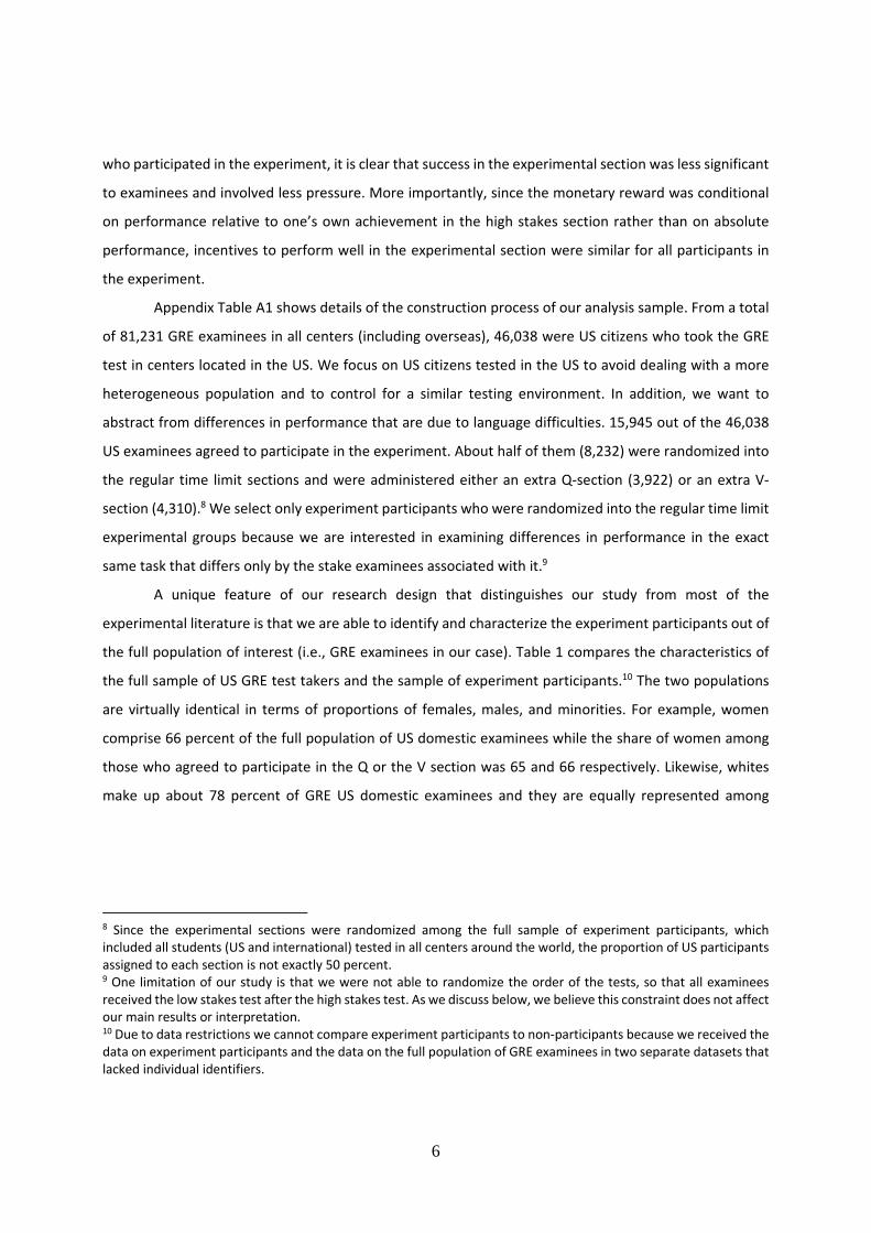
who participated in the experiment, it is clear that success in the experimental section was less significant
to examinees and involved less pressure. More importantly, since the monetary reward was conditional
on performance relative to one’s own achievement in the high stakes section rather than on absolute
performance, incentives to perform well in the experimental section were similar for all participants in
the experiment.
Appendix Table A1 shows details of the construction process of our analysis sample. From a total
of 81,231 GRE examinees in all centers (including overseas), 46,038 were US citizens who took the GRE
test in centers located in the US. We focus on US citizens tested in the US to avoid dealing with a more
heterogeneous population and to control for a similar testing environment. In addition, we want to
abstract from differences in performance that are due to language difficulties. 15,945 out of the 46,038
US examinees agreed to participate in the experiment. About half of them (8,232) were randomized into
the regular time limit sections and were administered either an extra Q‐section (3,922) or an extra V‐
section (4,310).8 We select only experiment participants who were randomized into the regular time limit
experimental groups because we are interested in examining differences in performance in the exact
same task that differs only by the stake examinees associated with it.9
A unique feature of our research design that distinguishes our study from most of the
experimental literature is that we are able to identify and characterize the experiment participants out of
the full population of interest (i.e., GRE examinees in our case). Table 1 compares the characteristics of
the full sample of US GRE test takers and the sample of experiment participants.10 The two populations
are virtually identical in terms of proportions of females, males, and minorities. For example, women
comprise 66 percent of the full population of US domestic examinees while the share of women among
those who agreed to participate in the Q or the V section was 65 and 66 respectively. Likewise, whites
make up about 78 percent of GRE US domestic examinees and they are equally represented among
8 Since the experimental sections were randomized among the full sample of experiment participants, which included all students (US and international) tested in all centers around the world, the proportion of US participants assigned to each section is not exactly 50 percent. 9 One limitation of our study is that we were not able to randomize the order of the tests, so that all examinees received the low stakes test after the high stakes test. As we discuss below, we believe this constraint does not affect our main results or interpretation. 10 Due to data restrictions we cannot compare experiment participants to non‐participants because we received the data on experiment participants and the data on the full population of GRE examinees in two separate datasets that lacked individual identifiers.
7
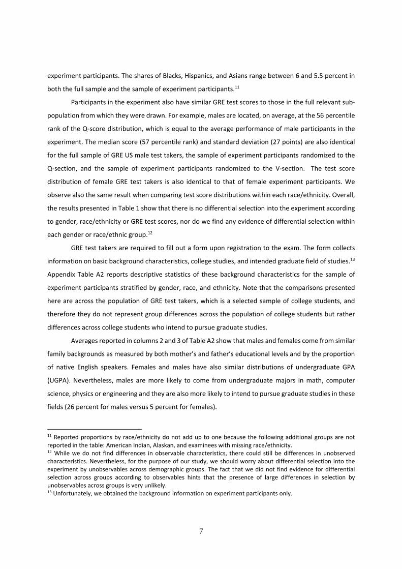
experiment participants. The shares of Blacks, Hispanics, and Asians range between 6 and 5.5 percent in
both the full sample and the sample of experiment participants.11
Participants in the experiment also have similar GRE test scores to those in the full relevant sub‐
population from which they were drawn. For example, males are located, on average, at the 56 percentile
rank of the Q‐score distribution, which is equal to the average performance of male participants in the
experiment. The median score (57 percentile rank) and standard deviation (27 points) are also identical
for the full sample of GRE US male test takers, the sample of experiment participants randomized to the
Q‐section, and the sample of experiment participants randomized to the V‐section. The test score
distribution of female GRE test takers is also identical to that of female experiment participants. We
observe also the same result when comparing test score distributions within each race/ethnicity. Overall,
the results presented in Table 1 show that there is no differential selection into the experiment according
to gender, race/ethnicity or GRE test scores, nor do we find any evidence of differential selection within
each gender or race/ethnic group.12
GRE test takers are required to fill out a form upon registration to the exam. The form collects
information on basic background characteristics, college studies, and intended graduate field of studies.13
Appendix Table A2 reports descriptive statistics of these background characteristics for the sample of
experiment participants stratified by gender, race, and ethnicity. Note that the comparisons presented
here are across the population of GRE test takers, which is a selected sample of college students, and
therefore they do not represent group differences across the population of college students but rather
differences across college students who intend to pursue graduate studies.
Averages reported in columns 2 and 3 of Table A2 show that males and females come from similar
family backgrounds as measured by both mother’s and father’s educational levels and by the proportion
of native English speakers. Females and males have also similar distributions of undergraduate GPA
(UGPA). Nevertheless, males are more likely to come from undergraduate majors in math, computer
science, physics or engineering and they are also more likely to intend to pursue graduate studies in these
fields (26 percent for males versus 5 percent for females).
11 Reported proportions by race/ethnicity do not add up to one because the following additional groups are not reported in the table: American Indian, Alaskan, and examinees with missing race/ethnicity. 12 While we do not find differences in observable characteristics, there could still be differences in unobserved characteristics. Nevertheless, for the purpose of our study, we should worry about differential selection into the experiment by unobservables across demographic groups. The fact that we did not find evidence for differential selection across groups according to observables hints that the presence of large differences in selection by unobservables across groups is very unlikely. 13 Unfortunately, we obtained the background information on experiment participants only.
8
Columns 3 through 6 in Table A2 report descriptive statistics of the analysis sample stratified by
race/ethnicity. Maternal education is similar among Whites and Asians but Asians are more likely to have
a father with at least some graduate studies or a professional degree relative to Whites (45 versus 35
percent). Hispanics and Blacks come from less educated families. Asians are less likely to be native English
speakers (86 percent) relative to Whites (93 percent), Blacks (95 percent), and Hispanics (90 percent). In
terms of undergraduate achievement, we observe that Whites and Asians have similar UGPAs
distributions but Hispanics and Blacks have, on average, lower UGPAs. Asians are more likely to do math,
science, and engineering either as an undergraduate major or as an intended field of graduate studies (30
percent) relative to Whites (11 percent), Blacks (8 percent), or Hispanics (12 percent).
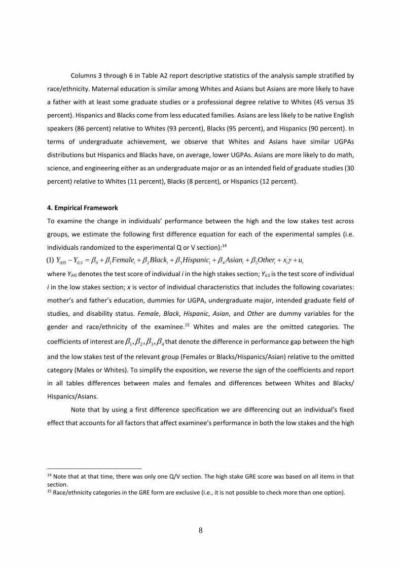
4. Empirical Framework
To examine the change in individuals’ performance between the high and the low stakes test across
groups, we estimate the following first difference equation for each of the experimental samples (i.e.
individuals randomized to the experimental Q or V section):14
where YiHS denotes the test score of individual i in the high stakes section; YiLS is the test score of individual
i in the low stakes section; x is vector of individual characteristics that includes the following covariates:
mother’s and father’s education, dummies for UGPA, undergraduate major, intended graduate field of
studies, and disability status. Female, Black, Hispanic, Asian, and Other are dummy variables for the
gender and race/ethnicity of the examinee.15 Whites and males are the omitted categories. The
coefficients of interest are 1 2 3 4, , , that denote the difference in performance gap between the high
and the low stakes test of the relevant group (Females or Blacks/Hispanics/Asian) relative to the omitted
category (Males or Whites). To simplify the exposition, we reverse the sign of the coefficients and report
in all tables differences between males and females and differences between Whites and Blacks/
Hispanics/Asians.
Note that by using a first difference specification we are differencing out an individual’s fixed
effect that accounts for all factors that affect examinee’s performance in both the low stakes and the high
14 Note that at that time, there was only one Q/V section. The high stake GRE score was based on all items in that section. 15 Race/ethnicity categories in the GRE form are exclusive (i.e., it is not possible to check more than one option).
'0 1 2 3 4 5(1) iHS iLS i i i i i i iY Y Female Black Hispanic Asian Other x u
9
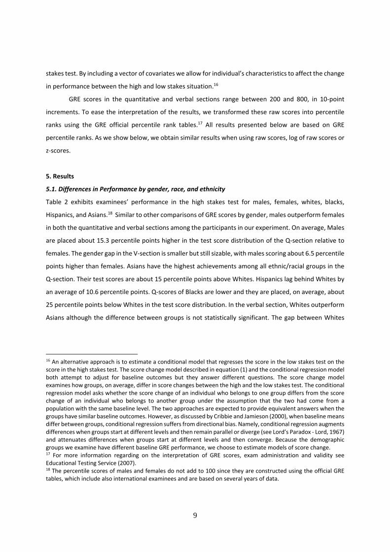
stakes test. By including a vector of covariates we allow for individual’s characteristics to affect the change
in performance between the high and low stakes situation.16
GRE scores in the quantitative and verbal sections range between 200 and 800, in 10‐point
increments. To ease the interpretation of the results, we transformed these raw scores into percentile
ranks using the GRE official percentile rank tables.17 All results presented below are based on GRE
percentile ranks. As we show below, we obtain similar results when using raw scores, log of raw scores or
z‐scores.
5. Results
5.1. Differences in Performance by gender, race, and ethnicity
Table 2 exhibits examinees’ performance in the high stakes test for males, females, whites, blacks,
Hispanics, and Asians.18 Similar to other comparisons of GRE scores by gender, males outperform females
in both the quantitative and verbal sections among the participants in our experiment. On average, Males
are placed about 15.3 percentile points higher in the test score distribution of the Q‐section relative to
females. The gender gap in the V‐section is smaller but still sizable, with males scoring about 6.5 percentile
points higher than females. Asians have the highest achievements among all ethnic/racial groups in the
Q‐section. Their test scores are about 15 percentile points above Whites. Hispanics lag behind Whites by
an average of 10.6 percentile points. Q‐scores of Blacks are lower and they are placed, on average, about
25 percentile points below Whites in the test score distribution. In the verbal section, Whites outperform
Asians although the difference between groups is not statistically significant. The gap between Whites
16 An alternative approach is to estimate a conditional model that regresses the score in the low stakes test on the score in the high stakes test. The score change model described in equation (1) and the conditional regression model both attempt to adjust for baseline outcomes but they answer different questions. The score change model examines how groups, on average, differ in score changes between the high and the low stakes test. The conditional regression model asks whether the score change of an individual who belongs to one group differs from the score change of an individual who belongs to another group under the assumption that the two had come from a population with the same baseline level. The two approaches are expected to provide equivalent answers when the groups have similar baseline outcomes. However, as discussed by Cribbie and Jamieson (2000), when baseline means differ between groups, conditional regression suffers from directional bias. Namely, conditional regression augments differences when groups start at different levels and then remain parallel or diverge (see Lord’s Paradox ‐ Lord, 1967) and attenuates differences when groups start at different levels and then converge. Because the demographic groups we examine have different baseline GRE performance, we choose to estimate models of score change. 17 For more information regarding on the interpretation of GRE scores, exam administration and validity see Educational Testing Service (2007). 18 The percentile scores of males and females do not add to 100 since they are constructed using the official GRE tables, which include also international examinees and are based on several years of data.
10
and Blacks is a bit smaller (23 percentile points) while the gap between Whites and Hispanics is about 12
percentile points.
Table 3 reports the change in performance between the high and the low stakes section for each
demographic group (first row of each panel) and the difference (second and third row) in the drop in
performance between males and females or between whites and Blacks/Hispanics/Asians. Males’
performance drops by 11.6 percentile points from the high to the low stakes Q‐sections while females’
performance drops by only 7.1 points. The differential gap in performance between males and females is
4.5 percentile points (s.e.=0.784). That is, a switch from the high to the low stakes situation narrows the
gender gap in the quantitative test by about 4.5 percentile points, which is equivalent to a 30 percent
drop in the gender gap of the high stakes test. The differential change in performance remains almost
unchanged after controlling for individual’s background characteristics and academic ability. This finding
is important as it suggests that our results are unlikely to be driven by differences in family background
and ability.
We also find a similar gender gap in the V‐section. Males’ scores drop by 10.4 percentile points,
on average, while females’ scores drop by a smaller magnitude of 6.1 percentile points. That is, males’
scores drop by 4.3 percentile points (s.e.=0.783) more relative to females. Note that the proportional drop
in males’ performance is also larger than females’. Namely, males’ scores drop by 21 percent while
females’ scores drop by 18 percent in the Q‐section. Similarly, we find that males’ scores in the V‐section
drop by 17 percent while females’ scores drop by 11 percent.
The stratification by race/ethnicity shows that whites exhibit the largest drop in performance
between the high and the low stakes Q‐section. Whites’ performance drops by 9.4 percentile points, while
that of Asians drops by 7 percentile points, Blacks’ performance drops by 3 percentile points, and
Hispanics’ performance drops by 3.8 percentile points. Differences in the performance drop between
Whites and each of the minority groups are all significant. The controlled difference between Whites and
Blacks, after accounting for individual’s characteristics, is of 4.3 percentile points (s.e.=1.05). The
equivalent difference between Whites and Hispanics is 5.21 (s.e.=1.40) and the difference between
Whites and Asians is 3.2 (s.e.=1.70). In the verbal section, the performance drop from the high to the low
stakes section is larger for Whites than for Blacks (7.8 percentile points versus 2.3 percentile points). But
Hispanics and Asians exhibit a similar drop in performance to that of Whites. We suspect that the different
pattern obtained for Asians and Hispanics in the V‐section could be related to language dominance.
Overall, the evidence presented in Table 3 shows that males and Whites exhibit the largest drop
in performance between the high and the low stakes tests compared to females and minorities. Our
11
results are robust to nonlinear transformations and alternative definitions of the dependent variable as
reported in Appendix Table A3. In the first row of panels A and B, we report differences in performance
in the quantitative and verbal sections using raw scores (scaled between 200 and 800). In the second row
of each panel, we show differences in performance using the natural logarithm of raw scores. In the third
row, we report results based on z‐scores.19 All alternative metrics yield results that are equivalent to our
main findings: males’ drop in performance between the high and low stakes section is 5 percent or .17 SD
larger than the drop of females; whites’ drop in performance in the Q‐section is 8 percent or .23 SD larger
than the drop of blacks; 7 percent or .23 SD larger than the drop of Hispanics and 7 percent or .19 SD
larger than the drop of Asians. These additional results show that our findings are not driven by a specific
scale used to measure achievement. Furthermore, as we show in Figure 1, we obtain the same results
when we rely only on the ordinal information embedded in scores. The last row of each panel replicates
our main results using the samples of examinees randomized into experimental sections with extended
time limit (67.5 minutes for the Q‐section and 45 minutes for the V‐section). Estimates are similar to our
main results showing that our findings are replicable in additional settings. In addition, they also show
that our results are not sensitive to time constraints or differential responses by gender or ethnicity to
the length of the exam.
5.2 Within Race/Ethnicity and Gender Differences in Performance
We check for gender and race/ethnicity interactions by examining whether differences between males
and females appear across all race/ethnic groups and whether differences between Whites and minorities
show up for males and for females.20
Table 4 reports differences in performance between males and females within each race/ethnicity
group as well as differences between Whites and minorities for males and females separately. The table
also reports performance in the high and low stakes section for each gender and ethnicity/race group. We
focus here in the Q‐section as we think performance is less influenced by language constraints among
Hispanics and Asians. The results show that White males have the largest differential performance
between the high and the low stakes test compared to Black, Asian, and, Hispanic males. We obtain a
similar result for females with the exception of Asian females who behave similarly to White females.
19 Z‐scores are computed using the mean and standard deviation of the high stakes test. 20 The conclusions described in this subsection rely on samples that are stratified by gender and race/ethnicity and that are relatively small for Blacks, Hispanics, and Asians so the results should be taken with caution.
12
Comparisons between males and females within each race/ethnicity group reveal that males
exhibit a larger drop in performance relative to females among Whites, Blacks, and Hispanics although
differences between genders are only statistically significant among Whites. In contrast, we observe no
gender differences among Asians. Asian males and females have an average drop in performance between
the high and the low stakes test of 6 and 7 percentile points respectively. In fact, the drop observed among
females is even larger than the drop observed among males, but the difference is not statistically
significant.
5.3 Heterogeneous effects
Table 5 reports the gender gap in students’ performance in high and low stakes tests for different
subsamples stratified by undergraduate GPA (UGPA), student’s major, intended field of graduate studies,
and mother’s education. We focus on gender gap and not on gap by race/ethnicity since subgroups are
too small for that stratification. Panel A reports results for the Q‐section and panel B reports results for
the V‐section. Rows 1 through 5 in both panels present estimates for the samples stratified by UGPA. As
expected, students with higher UGPA have higher scores in both the high and the low stakes sections of
the quantitative and verbal exams. Males’ advantage in the high stakes test appears across all cells of the
UGPA distribution both in the quantitative and the verbal sections. Again, we observe that the gender gap
in performance is narrower in the low stakes section in each of the cells stratified by UGPAs and is even
insignificant when comparing performance in the V‐section between male and female students with an
UGPA of A, A‐ or B‐.
We see in columns 9 and 10 of the table that all students, regardless of their academic ability
(proxied by UGPA) exhibit a significant drop in performance between the high and the low stakes sections
(both the quantitative and the verbal).21 Males’ performance drop is larger than females’ drop across all
ability levels (see columns 11 and 12) and is evident both in absolute and percentage terms.
The next two rows of Table 5 (in both panels A and B) report the gender gap in performance for
the sample of students who majored in math, computer science, physics or engineering or who intend to
pursue graduate studies in one of these fields (to simplify the discussion we will call them math and
science students). We focus on these students to target a population of females that is expected to be
21 We use UGPA to stratify the sample by academic ability (instead of using the score in the high stakes section) because it is an independent measure of performance that is not related to the dependent variable.
13
highly selected and perhaps more driven to achievement.22 While females represent the majority among
the full population of GRE examinees (65 percent) they are a minority among math and science students
(26 percent). It is therefore interesting to examine whether we find the same results in a subsample where
selection by gender goes in the opposite direction.
As seen in columns 3 and 4 of table 5, achievement in the GRE Q‐section is much higher among
math and science students relative to the sample average and even relative to those students whose
UGPA is an “A”. Math and science students also attain higher scores in the V‐section relative to the sample
average but they score slightly lower compared to those students with an “A” UGPA. The gender gap in
the high stakes Q‐section among math and science students is smaller (8.7 percentile points) than the
gender gap in the full sample (15.3 percentile points), although we still observe that males have higher
achievement than females. The gender gap among those who intend to pursue graduate studies in these
fields is even narrower (7.1 percentile points) although still significant. Finally, there is no gender gap
achievement in the V high stakes section in the subsamples of math and science students.
Achievement of math and science students in the Q low stakes section is lower than in the high
stakes section but these students still perform better relative to other students in the low stakes section.
Consistent with our previous results, the gender gap in Q performance among math and science students
is narrower in the low stakes section relative to the high stakes section and is even insignificant. The
pattern for the V section is similar with math and science females even outperforming their male
counterparts in the low stakes V‐section.
Even in this subsample of high achieving students, the drop in performance between the high and
the low stakes test is larger for males (who reduce their performance by about 12‐13 percentile points in
both subjects) compared to females (who reduce their performance by 6‐7 percentile points in the Q
section and by 4‐5 percentile points in the V section). The larger drop in males’ performance is evident
both in absolute terms and relative to the outcome means in the high stakes test. The gender differences
in relative performance in these subsamples is about 5 percentile points in the Q section and 8 percentile
points in the V sections. Both gaps are statistically significant and do not change much after controlling
for examinees’ observed characteristics. This finding is important because it shows that the larger drop in
performance among men is found even in subsamples that exhibit no differences in performance in the
high stakes test.
22 We focus here in a more limited number of fields than the traditional STEM definition (e.g., we exclude biology) to select those fields that are predominately populated by males. Our results do not change when using the broader definition of STEM fields.
14
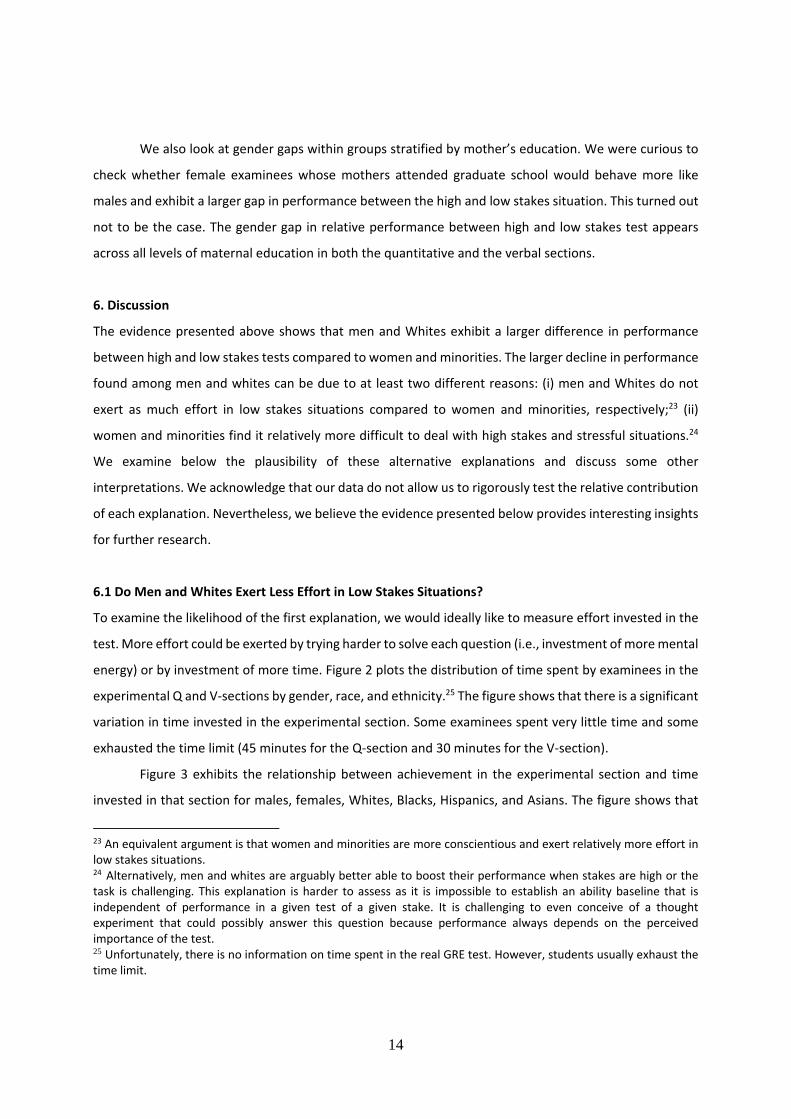
We also look at gender gaps within groups stratified by mother’s education. We were curious to
check whether female examinees whose mothers attended graduate school would behave more like
males and exhibit a larger gap in performance between the high and low stakes situation. This turned out
not to be the case. The gender gap in relative performance between high and low stakes test appears
across all levels of maternal education in both the quantitative and the verbal sections.
6. Discussion
The evidence presented above shows that men and Whites exhibit a larger difference in performance
between high and low stakes tests compared to women and minorities. The larger decline in performance
found among men and whites can be due to at least two different reasons: (i) men and Whites do not
exert as much effort in low stakes situations compared to women and minorities, respectively;23 (ii)
women and minorities find it relatively more difficult to deal with high stakes and stressful situations.24
We examine below the plausibility of these alternative explanations and discuss some other
interpretations. We acknowledge that our data do not allow us to rigorously test the relative contribution
of each explanation. Nevertheless, we believe the evidence presented below provides interesting insights
for further research.
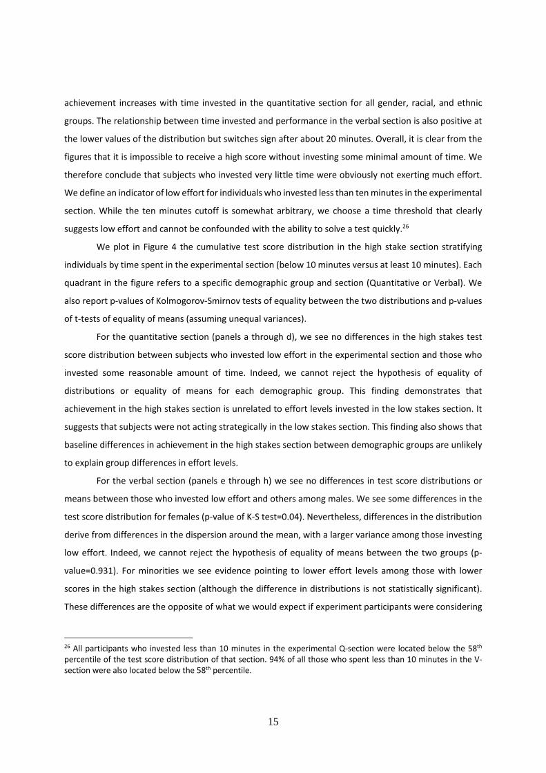
6.1 Do Men and Whites Exert Less Effort in Low Stakes Situations?
To examine the likelihood of the first explanation, we would ideally like to measure effort invested in the
test. More effort could be exerted by trying harder to solve each question (i.e., investment of more mental
energy) or by investment of more time. Figure 2 plots the distribution of time spent by examinees in the
experimental Q and V‐sections by gender, race, and ethnicity.25 The figure shows that there is a significant
variation in time invested in the experimental section. Some examinees spent very little time and some
exhausted the time limit (45 minutes for the Q‐section and 30 minutes for the V‐section).
Figure 3 exhibits the relationship between achievement in the experimental section and time
invested in that section for males, females, Whites, Blacks, Hispanics, and Asians. The figure shows that
23 An equivalent argument is that women and minorities are more conscientious and exert relatively more effort in low stakes situations. 24 Alternatively, men and whites are arguably better able to boost their performance when stakes are high or the task is challenging. This explanation is harder to assess as it is impossible to establish an ability baseline that is independent of performance in a given test of a given stake. It is challenging to even conceive of a thought experiment that could possibly answer this question because performance always depends on the perceived importance of the test. 25 Unfortunately, there is no information on time spent in the real GRE test. However, students usually exhaust the time limit.
15
achievement increases with time invested in the quantitative section for all gender, racial, and ethnic
groups. The relationship between time invested and performance in the verbal section is also positive at
the lower values of the distribution but switches sign after about 20 minutes. Overall, it is clear from the
figures that it is impossible to receive a high score without investing some minimal amount of time. We
therefore conclude that subjects who invested very little time were obviously not exerting much effort.
We define an indicator of low effort for individuals who invested less than ten minutes in the experimental
section. While the ten minutes cutoff is somewhat arbitrary, we choose a time threshold that clearly
suggests low effort and cannot be confounded with the ability to solve a test quickly.26
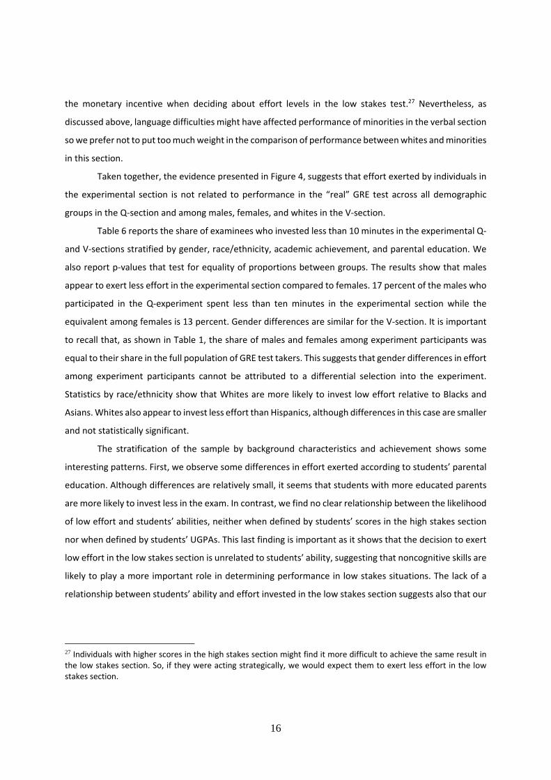
We plot in Figure 4 the cumulative test score distribution in the high stake section stratifying
individuals by time spent in the experimental section (below 10 minutes versus at least 10 minutes). Each
quadrant in the figure refers to a specific demographic group and section (Quantitative or Verbal). We
also report p‐values of Kolmogorov‐Smirnov tests of equality between the two distributions and p‐values
of t‐tests of equality of means (assuming unequal variances).
For the quantitative section (panels a through d), we see no differences in the high stakes test
score distribution between subjects who invested low effort in the experimental section and those who
invested some reasonable amount of time. Indeed, we cannot reject the hypothesis of equality of
distributions or equality of means for each demographic group. This finding demonstrates that
achievement in the high stakes section is unrelated to effort levels invested in the low stakes section. It
suggests that subjects were not acting strategically in the low stakes section. This finding also shows that
baseline differences in achievement in the high stakes section between demographic groups are unlikely
to explain group differences in effort levels.
For the verbal section (panels e through h) we see no differences in test score distributions or
means between those who invested low effort and others among males. We see some differences in the
test score distribution for females (p‐value of K‐S test=0.04). Nevertheless, differences in the distribution
derive from differences in the dispersion around the mean, with a larger variance among those investing
low effort. Indeed, we cannot reject the hypothesis of equality of means between the two groups (p‐
value=0.931). For minorities we see evidence pointing to lower effort levels among those with lower
scores in the high stakes section (although the difference in distributions is not statistically significant).
These differences are the opposite of what we would expect if experiment participants were considering
26 All participants who invested less than 10 minutes in the experimental Q‐section were located below the 58th percentile of the test score distribution of that section. 94% of all those who spent less than 10 minutes in the V‐section were also located below the 58th percentile.
16
the monetary incentive when deciding about effort levels in the low stakes test.27 Nevertheless, as
discussed above, language difficulties might have affected performance of minorities in the verbal section
so we prefer not to put too much weight in the comparison of performance between whites and minorities
in this section.
Taken together, the evidence presented in Figure 4, suggests that effort exerted by individuals in
the experimental section is not related to performance in the “real” GRE test across all demographic
groups in the Q‐section and among males, females, and whites in the V‐section.
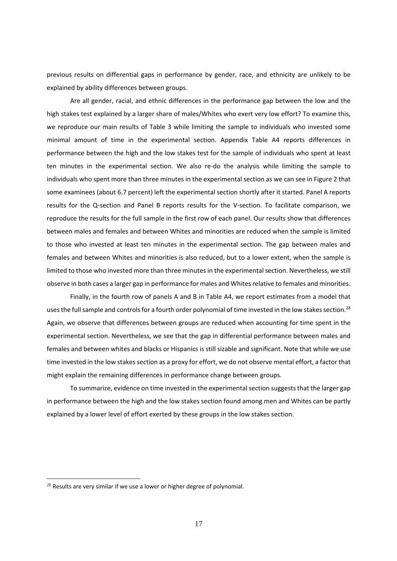
Table 6 reports the share of examinees who invested less than 10 minutes in the experimental Q‐
and V‐sections stratified by gender, race/ethnicity, academic achievement, and parental education. We
also report p‐values that test for equality of proportions between groups. The results show that males
appear to exert less effort in the experimental section compared to females. 17 percent of the males who
participated in the Q‐experiment spent less than ten minutes in the experimental section while the
equivalent among females is 13 percent. Gender differences are similar for the V‐section. It is important
to recall that, as shown in Table 1, the share of males and females among experiment participants was
equal to their share in the full population of GRE test takers. This suggests that gender differences in effort
among experiment participants cannot be attributed to a differential selection into the experiment.
Statistics by race/ethnicity show that Whites are more likely to invest low effort relative to Blacks and
Asians. Whites also appear to invest less effort than Hispanics, although differences in this case are smaller
and not statistically significant.
The stratification of the sample by background characteristics and achievement shows some
interesting patterns. First, we observe some differences in effort exerted according to students’ parental
education. Although differences are relatively small, it seems that students with more educated parents
are more likely to invest less in the exam. In contrast, we find no clear relationship between the likelihood
of low effort and students’ abilities, neither when defined by students’ scores in the high stakes section
nor when defined by students’ UGPAs. This last finding is important as it shows that the decision to exert
low effort in the low stakes section is unrelated to students’ ability, suggesting that noncognitive skills are
likely to play a more important role in determining performance in low stakes situations. The lack of a
relationship between students’ ability and effort invested in the low stakes section suggests also that our
27 Individuals with higher scores in the high stakes section might find it more difficult to achieve the same result in the low stakes section. So, if they were acting strategically, we would expect them to exert less effort in the low stakes section.
17
previous results on differential gaps in performance by gender, race, and ethnicity are unlikely to be
explained by ability differences between groups.
Are all gender, racial, and ethnic differences in the performance gap between the low and the
high stakes test explained by a larger share of males/Whites who exert very low effort? To examine this,
we reproduce our main results of Table 3 while limiting the sample to individuals who invested some
minimal amount of time in the experimental section. Appendix Table A4 reports differences in
performance between the high and the low stakes test for the sample of individuals who spent at least
ten minutes in the experimental section. We also re‐do the analysis while limiting the sample to
individuals who spent more than three minutes in the experimental section as we can see in Figure 2 that
some examinees (about 6.7 percent) left the experimental section shortly after it started. Panel A reports
results for the Q‐section and Panel B reports results for the V‐section. To facilitate comparison, we
reproduce the results for the full sample in the first row of each panel. Our results show that differences
between males and females and between Whites and minorities are reduced when the sample is limited
to those who invested at least ten minutes in the experimental section. The gap between males and
females and between Whites and minorities is also reduced, but to a lower extent, when the sample is
limited to those who invested more than three minutes in the experimental section. Nevertheless, we still
observe in both cases a larger gap in performance for males and Whites relative to females and minorities.
Finally, in the fourth row of panels A and B in Table A4, we report estimates from a model that
uses the full sample and controls for a fourth order polynomial of time invested in the low stakes section.28
Again, we observe that differences between groups are reduced when accounting for time spent in the
experimental section. Nevertheless, we see that the gap in differential performance between males and
females and between whites and blacks or Hispanics is still sizable and significant. Note that while we use
time invested in the low stakes section as a proxy for effort, we do not observe mental effort, a factor that
might explain the remaining differences in performance change between groups.
To summarize, evidence on time invested in the experimental section suggests that the larger gap
in performance between the high and the low stakes section found among men and Whites can be partly
explained by a lower level of effort exerted by these groups in the low stakes section.
28 Results are very similar if we use a lower or higher degree of polynomial.
18
6.2 Are Women and Minorities More Subject to Stress in High Stakes Situations?
As noted above, a second possible explanation for the larger gap in performance between the high and
the low stakes section among men and Whites could be a higher level of stress and test anxiety among
females and minorities that hinders their performance in high stakes situations. To examine this
explanation, we inspect the distribution of changes in performance between the high and the low stakes
test. Although most individuals have lower test scores in the low stakes section, we find that some
students do improve their performance. This improvement can be due to the volatility of, or measurement
error, in test scores, due to learning or increased familiarity with the test, or due to a lower level of stress
and anxiety involved in the low stakes test. We adjust for score volatility and compare the share of
examinees who improved their performance across demographic groups.
Columns 1 and 6 of table 7 report the share of examinees who improved their scores in the
quantitative and in the verbal experimental sections. To adjust for score improvement due to score
volatility and measurement error, we define a score gain for cases where the difference between the low‐
stakes score and the high‐stakes score divided by the conditional standard error of measurement of
difference scores is greater than 1.65.29 Roughly 1.5 percent of examinees have a significant score gain in
the experimental Q‐section and 5.3 percent in the V‐section. Columns 2 through 5 and 7 through 10 report
differences in the share of examinees who improve scores by gender and by race/ethnicity. The first row
reports raw differences between groups, the second row reports differences after controlling for
students’ background characteristics, and the third row reports odds ratios between females/minorities
and males/whites. Overall, we find very small and insignificant differences in the likelihood of improving
the score by gender. Odds ratios are close to one for both sections (i.e. small effect size) meaning that the
odds of improving the score for males and females are similar. With the exception of Hispanics in the
quantitative section and Blacks in the verbal section, all other differences between whites and minorities
are small and insignificant with odds ratios that are close to one.
We further explore the differential impact of test anxiety across groups using an alternative
approach that takes advantage of additional information reported by examinees in the background
questionnaire. The questionnaire asked examinees to report the reason(s) for taking the GRE test,
allowing them to mark various alternatives. About 7 percent marked “practice” as one of the reasons for
29 We use the conditional standard error of measurement of difference scores reported in Table 6b of the official ETS publication and define an indicator for score improvement following the ETS definition of significant GRE score differences (see ETS, 2007).
19
taking the exam.30 If test anxiety hinders performance of females, blacks or Hispanics relative to males or
whites in the high stakes section, we expect to find smaller group differences in the performance drop
between the high to the low stakes section among those taking the test for practice.31 To examine this,
we estimated our basic model of drop in performance (as in Table 3) while adding interactions between
an indicator for taking the test for practice and the demographic groups. Estimates reported in Table 8
show that the gap between demographic groups among those taking the exam for practice is not smaller
than the gap estimated among those who are taking the exam for admission to graduate school or
fellowship application and are probably facing a more stressing situation.
Taken together, the evidence presented in Tables 7 and 8 suggests that test anxiety in the high
stakes section is unlikely to be the reason for the smaller change in performance between the high and
the low stakes tests observed among females and minorities.
6.3. Other Explanations
An additional explanation for our results could be that the monetary prize offered to experiment
participants had a differential impact on different demographic groups. While this is possible, we note
that the prize consisted of $250 (1.5 times the GRE cost) paid to 100 individuals out of 30,000 experiment
participants. Such an amount distributed to such a small number of participants seems too low to have a
significant differential effect in performance. Alternatively, it is arguably the case that differences in
performance in the experimental section arises from group differences in their opportunity cost of time.
However, as shown in Table 1, participation rates in the experiment were similar across demographic
groups, suggesting that there were no group differences in the perceived cost or benefit of participating
in the experiment.
To further assess the impact of the monetary prize and the opportunity cost of time on performance
in the experimental section, we examined the association between the change in performance (from the
high to the low stakes section) and earning levels at the state of residence of the examinee. We use two
different measures of earnings: median annual earnings of full time workers and median annual earnings
30 The main reasons were admission to graduate school (96%) and graduate department admissions requirement (29%). Other reasons include fellowship/scholarship application requirement (23%), undergraduate program exit requirement (1%), and other (3%). Applicants were instructed to select all reasons that apply, so that reasons do not add up to 100%. The background questionnaire is filled by examinees before the test so it is not affected by their performance. 31 Students who took the exam for practice might be different from those who took the exam for university admission. However, for the purpose of our comparison, we only need to assume that selection works in a similar direction for all demographic groups.
20
of college graduates computed separately by gender and state.32 If the monetary prize or the opportunity
cost of time had any impact on performance at the experimental section, we should expect a smaller
reduction in performance in states with lower earnings levels. We report in Appendix Table A7, regression
estimates for the association between the change in performance and median earnings for males and
females. Columns 1 and 3 report estimates from simple bivariate models and columns 2 and 4 report
estimates from regressions that control for examinee characteristics. Overall, we do not find any
association between median earnings at the state of residence of the examinee and his/her change in
performance suggesting that our main results are unlikely to be explained by a differential impact of the
monetary prize or the opportunity cost of time.
Another alternative explanation for differential changes in performance could be that performance
of females and minorities is lower than expected in the high stakes section due to stereotype threat (e.g.
Steele, 1997 and Steel and Aronson, 1995). However, it is unclear why gender and race/ethnicity
stereotypes would be more pronounced in the high stakes section. In addition, the fact that we find similar
gender differences in both the quantitative and the verbal sections suggest that stereotype threat is
unlikely to explain our main results as the theory would predict that females would respond negatively
only to the quantitative section. Moreover, stereotype threat theory implies that Asians should respond
differently than Blacks and Hispanics in the quantitative section but our findings are similar for the three
groups.
We further assess the likelihood of stereotype threat explanation by examining the relationship
between gender stereotypes in math and verbal achievement at the state of residence of the examinees
and the differential change in performance. To proxy for gender stereotypes at the state of residence of
the examinee we use the stereotype adherence index developed by Pope and Sydnor (2010) which
reflects gender disparities in test scores favoring boys in math and science and favoring girls in reading
and was shown by the authors to be positively associated with other measures of gender stereotype
attitudes at the state level.33 Higher values in this index mean a stronger gender stereotype. To facilitate
interpretation of the results, we transform this index into a z‐score. We hypothesize that stereotype threat
plays a more important role in states with higher values in the stereotype index. Therefore, for our results
32 Earnings come from data published by the U.S. Census Bureau based on 5‐year average earnings by state and gender from American Community Survey for the years 2005‐2008. 33 Pope and Sydnor (2010) use test score data from the National Assessment of Educational Progress (NAEP) and show that states that have larger gender disparities in stereotypically male‐dominated tests of math and science also tend to have larger gender disparities (of the opposite sign) in stereotypically female‐dominated tests of reading. The authors develop a state stereotype adherence index that is defined as the average of the male‐female ratio in math and science and female‐male ratio in reading for the top 5 percent of the students.
21
to be consistent with stereotype threat, we should observe a larger gender differential in the Q‐section
and a smaller gender differential in the V‐section in states with a higher stereotype index. In Appendix
Table A6, we examine this hypothesis by regressing the score difference between the high and the low
stakes section on a female indicator, the gender stereotype index and an interaction between these two
variables. Estimates for the interaction term between female and the stereotype index are all small and
insignificant, meaning that there is no apparent relationship between state gender stereotypes and the
gender gap in differential performance between the high and the low stakes section. Moreover, their sign
goes in the opposite direction than would be expected by the stereotype threat theory.
An additional alternative interpretation of our findings could be that group differences in underlying
ability might generate differential drop in performance. However, as we note above, we observe the same
pattern of gender and race/ethnic differences across different subsamples and even in subsamples that
exhibit similar performance in the high or the low stakes section.
Because examinees participated in the experimental section after they completed the real GRE
examination, it is also possible that our results are due to the fact that women and minorities become less
fatigued by the GRE examination than men and Whites, respectively. This argument seems unlikely as it
goes against recent psychological and medical literature that claims that, if anything, females appear to
exhibit a higher level of fatigue after performance of cognitive tasks (see, e.g., Yoon et al., 2009). In
addition, we are not aware of any studies that show that Whites exhibit a higher level of fatigue in
response to cognitive tasks compared to Blacks, Hispanics, or Asians. Furthermore, in the context of
aptitude tests, Ackerman and Kanfer (2009) and Liu et al. (2004) show no evidence for a decline in test
performance in the longer test conditions. Moreover, the fact that we find similar participation rates in
the experiment among males and females and whites, blacks, Hispanics, and Asians, provides further
evidence that a differential effect of fatigue is unlikely to explain our findings. Lastly, as shown in Appendix
table A4, the fact that we can replicate our results in the samples of students randomized into the
extended time limit sections, provides strong evidence that mitigates this concern.
Finally, one could argue that group differences in performance change between the low and the
high stakes section can be explained by differences in learning or test familiarization. To assess this
conjecture, we took advantage of one additional piece of information at our disposal. The background
questionnaire collected information on examinees’ preparation methods for the GRE exam (e.g., use of
software or books published by the ETS or other providers, coaching courses offered by commercial
companies, coaching courses offered by educational institutions, no preparation, etc.). We coded this
information in a vector of dummy variables and re‐estimated our main models while controlling for these
22
additional covariates. Results of these expanded models are reported in Appendix Table A7 together with
results from our main specification. All estimates are highly similar to our main results suggesting that
learning or test familiarization cannot explain our findings.
7. Conclusions
In this study we examine the differential performance of females, males, Whites, and minorities in low
and high stakes situations by comparing the performance of GRE examinees in the real and in an
experimental section of the test. Our results show that males and Whites have the highest differential
change in performance relative to females, Asians, Hispanics, and Blacks. Males’ drop in performance
between the high and low stakes section is .16 SD larger than the drop of females; whites’ drop in
performance in the Q‐section is .23 SD larger than the drop of blacks and the drop of Hispanics, and .19
SD larger than the drop of Asians. We show that the larger differential performance observed among
males and Whites is partially due to the fact that these two groups invest less effort in the low stakes test.
We rule out alternative explanations for these findings such as stereotype threat, differences in stress
levels, learning or alternative cost of time.
Our findings suggest that men and Whites who perform well in high stake tests might not perform
as well in ordinary assignments, and that women and minorities who do not perform so well in high stake
tests may do relatively better in low stakes tasks. Our findings demonstrate that test score gaps between
males and females or between Whites and minorities might vary according to the stakes of the test, as
each group appears to respond differently to level of stakes. Therefore, it is important to consider the
stakes of a test and the differential performance of each group according to the stakes level when
analyzing test score gaps. We show this in Appendix Table A8 where we compare the (low stakes) NAEP
test scores in mathematics that was administered to 12th grade students in 2015 to the (high stakes) SAT
scores at 2015. Consistent with our results, we see that test score gaps between males and females, and
Whites and Blacks, Whites and Hispanics and Whites and Asians are larger at the SAT compared to the
NAEP. Our results are also consistent with the claim that standardized tests usually underpredict college
and graduate school performance for women and overpredict performance for men (see, e.g., Willingham
and Cole, 1997 and Rothstein, 2004).34
34 Our findings also suggest the same pattern for Whites compared to minorities, but this is not the case in practice (see, e.g., Mattern et al., 2008), presumably because the lower performance of minority students in college can be explained by other factors such as their relatively disadvantaged background (Rothstein, 2004).
23
It is interesting to try to determine to what extent differences in performance between high and
low stakes situations are socially constructed or innate. While this question is beyond the scope of the
current study, we speculate that the similarity between Asian males and females suggests that part of the
source for the gender differences observed among other ethnic and racial groups might be explained by
acquired rather than innate skills.
A curious finding that relates to this question is presented in Figure 5, where we plot differences in
achievement between the high and the low stakes Q‐section by students’ undergraduate major.
Interestingly, those who exhibit the largest gap in achievement between the high and the low stakes
section are economics majors. This finding could be either a result of self‐selection into economic majors
or skills acquired during undergraduate studies. Be that as it may, it is consistent with Rubinstein (2006)
who finds that economics majors have a much stronger tendency to maximize profits relative to other
undergraduate majors.
Our results may also have implications for admission policies that are intended to achieve
demographic diversity in educational institutions and the workplace. If different groups perform
differently in low and high stakes situations, then policymakers may be able to diversify the population
admitted to colleges, universities, specific study fields, and workplaces by gentle manipulation of the
stakes of admission exams. There are several different possible mechanisms that may help facilitate such
a change. For example, allowing students to retake an admission test and consideration of the average or
the maximum score obtained would reduce the stake of any given test.35
Finally, our results may also have implications for personnel and incentive policies as they suggest
that differences in productivity between workers could vary according to the incentive scheme attached
to the job. Often times, job candidates are evaluated using high stake tests. However, most jobs require
excellence in tasks that are not directly attached to high‐powered incentive schemes. This suggests that
consideration of performance in high stake tests should not come at the expense of consideration of other
indicators of ability that reflect good performance in low stake situations.
35 Indeed, this type of policy has recently been adopted for the SAT and GRE. The new policy, known as Score Choice, gives students the option to choose the SAT scores to be sent to colleges by test date and subject (CollegeBoard, 2009). The ETS has also established in 2012 a new policy known as ScoreSelect that allows test takers to report all, none or some of their test scores to graduate programs. While this policy is expected to lower the level of stress and stakes of any given test, Vigdor and Clotfelter (2001) show that minority students are less likely to retake the SAT; a fact that might offset the possible benefits of this policy.
24
References
Ackerman P. L. and R. Knafer, (2009) “Test Length and Cognitive Fatigue: an Empirical Examination of
Effects of Performance and Test‐Taker Reactions”, Journal of Experimental Psychology: Applied, Vol.
15 No.2, pp. 163‐181.
Ariely, D., Gneezy U., and G. Loewenstein (2009) “Large Stakes and Big Mistakes”, Review of Economic
Studies, Vol. 76, pp. 451‐469.
Barres, B. (2006) “Does Gender Matter?” Nature, No. 442, pp. 133‐136.
Booth, A. and P. Nolen (2011) “Choosing To Compete: How Different Are Girls and Boys?” Forthcoming,
Journal of Economic Behavior and Organization.
Booth, A. and P. Nolen (2012) “Gender Differences in Risk Behavior: Does Nurture Matter” Forthcoming,
Economic Journal.
Borghans, L. H. Meijers, and B. T. Weel (2008), “The Role of Noncognitive Skills in Explaining Cognitive Test
Scores” Economic Inquiry, Vol. 46 No. 1, pp. 2‐12.
Bridgeman B., F. Cline, and J. Hessinger (2004) “Effect of Extra Time on Verbal and Quantitative GRE
Scores” Journal Applied Measurement in Education No. 17, pp. 25‐37.
Cassaday, J. C., and Johnson, R. E. (2002) “Cognitive Test Anxiety and Academic Performance”
Contemporary Educational Psychology, 27, 270–295.
Cole, J. S., D. A. Bergin, and T. A. Whittaker (2008) “Predicting student achievement for low stakes test
with effort and task value” Contemporary Educational Psychology No. 33, pp. 609‐624.
CollegeBoard (2009). SAT Score‐Use Practices by Participating Institution.
Cotton, C., F. McIntyre, and J. Price (2010) “The Gender Gap Under Pressure: A Detailed Look at Male and
Female Performance Differences During Competitions” NBER Working Paper No. 16436.
Cribbie, R. A. and J. Jamieson, (2000) “Structural Equation and the Regression Bias for Measuring
Correlates of Change”, Educational and Psychological Measurement, Vol. 60 No. 6, pp. 893‐907.
Datta Gupta, N., A. Poulsen, and M. C. Villeval (2005) “Male and Female Competitive Behavior:
Experimental Evidence” IZA Discussion Paper No. 1833.
Dohmen, T. J. and A. Falk, (2011) “Performance Pay and Multi‐Dimensional Sorting: Productivity,
Preferences, and Gender”, American Economic Review, Vol. 101, No. 2, pp. 493‐525.
25
Duckworth, A. L., and M. E. P. Seligman (2006) “Self‐discipline gives girls the edge: Gender in self‐
discipline, grades, and achievement test scores” Journal of Educational Psychology, Vol. 98 No. 1, pp.
198‐208.
Educational Testing Service, ETS (2007), “Graduate Record Examinations, Guide to the Use of Scores 2007‐
2008”.
Flory, J. A., A. Leibbrandt and J. A. List (2010) “Do Competitive Work Places Deter Female Workers? A
Large‐Scale Natural Experiment on Gender Differences in Job Entry Decisions” NBER Working Paper
No. 16546.
Gneezy, U., K. L. Leonard, and J. A. List (2009) “Gender Differences in Competition: Evidence From a
Matrilineal and a Patriarchal Society” Econometrica Vol. 77 No. 5, pp. 1637‐1664.
Gneezy, U., M. Niederle, and A. Rustichini (2003) “Performance in Competitive Environments: Gender
Differences” Quarterly Journal of Economics, Vol. 108 No. 3, pp. 1049‐1074.
Gneezy, U., and A. Rustichini (2004) “Gender and Competition at a Young Age” American Economic Review
Papers and Proceedings, Vol. 94 No. 2, pp. 377‐381.
Gunther, C., N. A. Ekinci, C. Schwieren, and M. Strobel, (2010) “Women Can’t Jump? An Experiment on
Competitive Attitudes and Stereotype Threat” Journal of Economic Behavior and Organization, Vol.
75 No. 3, pp. 395‐401.
Heckman, J. J. and Y. Rubinstein (2001), “The Importance of Noncognitive Skills: Lessons from the GED
Testing Program”, American Economic Review Papers and Proceedings, Vol. 91 No. 2, pp. 145‐149.
Heckman, J. J., and F. Cunha (2007), “The Technology of Skill Formation”, American Economic Review, Vol.
97 No. 2, pp. 31‐47.
Jurajda, Š. and D. Münich (2011), “Gender Gap in Admission Performance under Competitive Pressure”,
American Economic Review Papers and Proceedings, May.
Lavy, V. (2008) “Gender Differences in Competitiveness in a Real Workplace: Evidence from Performance‐
Based Pay Tournaments among Teachers.” NBER Working Paper 14338.
Liu J., J. R. Allspach, M. Feigenbaum, H. J. Oh, and N. Burton (2004) “A Study of Fatigue Effects from the
New SAT,” College Board Research Report No. 2004‐2005.
26
Lord F. M. (1967), “A Paradox in the Interpretation of Group Comparisons”, Psychological Bulletin, Vol. 68
No. 5, pp. 304‐305.
Mattern, K. D., B. F. Patterson, E. J. Shaw, J. L. Kobrin, and S. M. Barbuti (2008) “Differential Validity and
Prediction of the SAT” College Board Research Report No. 2008‐4, The College Board, New York,
2008.
Niederle, M., and L. Vesterlund (2007) “Do Women Shy Away From Competition? Do Men Compete Too
Much?” Quarterly Journal of Economics, Vol. 122 No. 3, pp. 1067‐1101.
Niederle, M., C. Segal, and L. Vesterlund (2008). “How Costly is Diversity? Affirmative Action in Light of
Gender Differences in Competitiveness”, NBER Working Paper No. 13922.
Niederle, M., and L. Vesterlund (2010). “Explaining the Gender Gap in Math Test Scores,” Journal of
Economic Perspectives, Vol. 24 No. 2, pp. 124‐144.
Niederle, M., and L. Vesterlund (2011). “Gender and Competition,” Annual Review of Economics, Vol. 3,
pp. 601‐30.
O’Neil, H. F., B. Sugrue, and E. L. Baker (1996) “Effects of Motivational Interventions on the National
Assessment of Educational Progress Mathematics Performance”, Educational Assessment, Vol. 2 No.
2, pp. 135‐157.
Örs, E., F. Palomino, and E. Peyrache (2008). “Performance Gender‐Gap: Does Competition Matter?” CEPR
Discussion Paper No. 6891.
Paarsch, H. and Bruce S. Shearer (2007) “Do Women React Differently to Incentives? Evidence from
Experimental Data and Payroll Records”, European Economic Review, Vol. 51, pp. 1682‐1707.
Paserman, D. (2010) “Gender Differences in Performance in Competitive Environments: Evidence from
Professional Tennis Players.” Discussion Paper, Boston University.
Pope, D. G. and J. R. Sydnor (2010), “Geographic Variation in the Gender Differences in Test Scores,”
Journal of Economic Perspectives, Vol. 24 No. 2, pp. 95‐108.
Rothstein, J. (2004), “College Performance Predictions and the SAT,” Journal of Econometrics, Vol. 121
No.1‐2, pp. 123‐144.
Rubinstein, A. (2006), “A Skeptic’s Comment on the Study of Economics”, Economic Journal, Vol. 116, C1‐
C9.
27
Segal, C., (2010), “Motivation, Test Scores, and Economic Success”, Working Paper, Universitat Pompeu
Fabra.
Shurchkov, Olga. (Forthcoming) “Under pressure: Gender Differences in Output Quality and Quantity
under Competition and Time Constraints,” Journal of the European Economic Association.
Spencer, S., Steele, C. M., and D. M. Quinn (1999) “Stereotype Threat and Women’s Math Performance,”
Journal of Experimental Social Psychology, Vol. 35 No. 1, pp. 4‐28.
Steele, C. M., (1997) “A threat in the Air: How Stereotypes Shape the Intellectual Identities and
Performance of Women and African‐Americans”, American Psychologist, Vol. 52 No. 6, pp. 613‐629.
Steele, C. M. and J. Aronson (1995) “Stereotype threat and the intellectual test performance of African
Americans”, Journal of Personality and Social Psychology, Vol. 69, pp. 797‐811.
Vigdor, J. L. and C. T. Clotfelter (2001), “Retaking the SAT” Journal of Human Resources, Vol. 38, pp. 1‐33.
Willingham, W.W., and N. S. Cole, N.S. (1997). Gender and fair assessment. Mahwah, NJ: Erlbaum.
Yoon T., M. Keller, B. Schinder De‐Lap, A. Harkins, R. Lepers, and S. Hunter, (2009) “Sex Differences in
Response to Cognitive Stress During a Fatiguing Contraction”, Journal of Applied Physiology, Vol. 107,
pp. 1486‐1496.
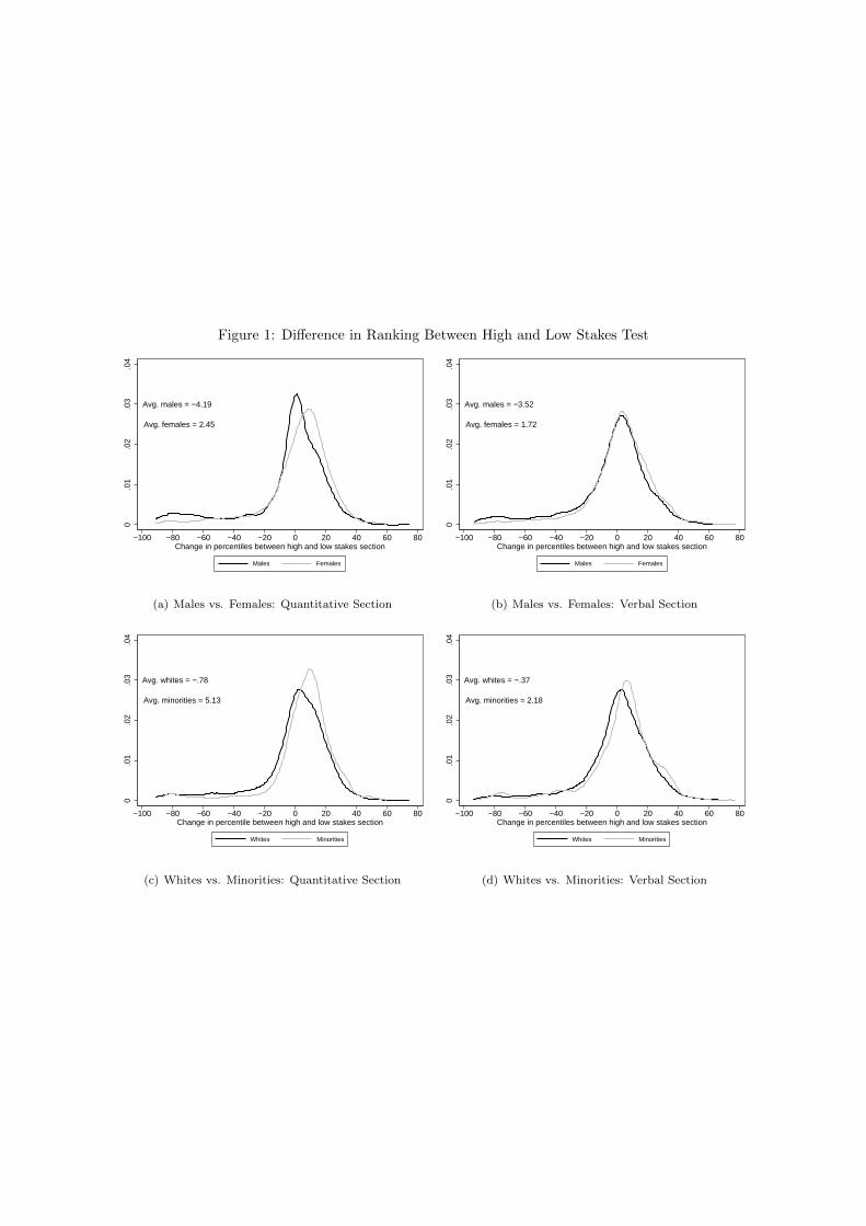
Figure 1: Difference in Ranking Between High and Low Stakes Test
Avg. males = −4.19
Avg. females = 2.45
0.0
1.0
2.0
3.0
4
−100 −80 −60 −40 −20 0 20 40 60 80Change in percentiles between high and low stakes section
Males Females
(a) Males vs. Females: Quantitative Section
Avg. males = −3.52
Avg. females = 1.72
0.0
1.0
2.0
3.0
4
−100 −80 −60 −40 −20 0 20 40 60 80Change in percentiles between high and low stakes section
Males Females
(b) Males vs. Females: Verbal Section
Avg. whites = −.78
Avg. minorities = 5.13
0.0
1.0
2.0
3.0
4
−100 −80 −60 −40 −20 0 20 40 60 80Change in percentile between high and low stakes section
Whites Minorities
(c) Whites vs. Minorities: Quantitative Section
Avg. whites = −.37
Avg. minorities = 2.18
0.0
1.0
2.0
3.0
4
−100 −80 −60 −40 −20 0 20 40 60 80Change in percentiles between high and low stakes section
Whites Minorities
(d) Whites vs. Minorities: Verbal Section
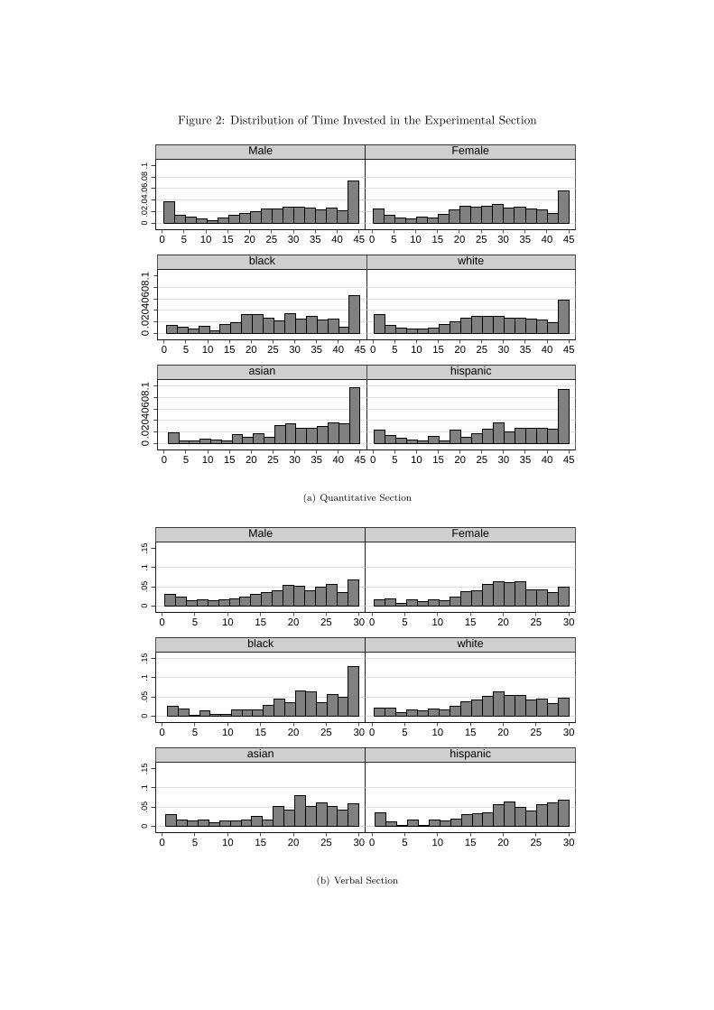
Figure 2: Distribution of Time Invested in the Experimental Section
0.0
2.04
.06.
08.1
0 5 10 15 20 25 30 35 40 45 0 5 10 15 20 25 30 35 40 45
Male Female0
.02.0
4.06.0
8.1
0 5 10 15 20 25 30 35 40 45 0 5 10 15 20 25 30 35 40 45
black white
0.0
2.04.0
6.08.
1
0 5 10 15 20 25 30 35 40 45 0 5 10 15 20 25 30 35 40 45
asian hispanic
(a) Quantitative Section
0.0
5.1
.15
0 5 10 15 20 25 30 0 5 10 15 20 25 30
Male Female
0.0
5.1
.15
0 5 10 15 20 25 30 0 5 10 15 20 25 30
black white
0.0
5.1
.15
0 5 10 15 20 25 30 0 5 10 15 20 25 30
asian hispanic
(b) Verbal Section
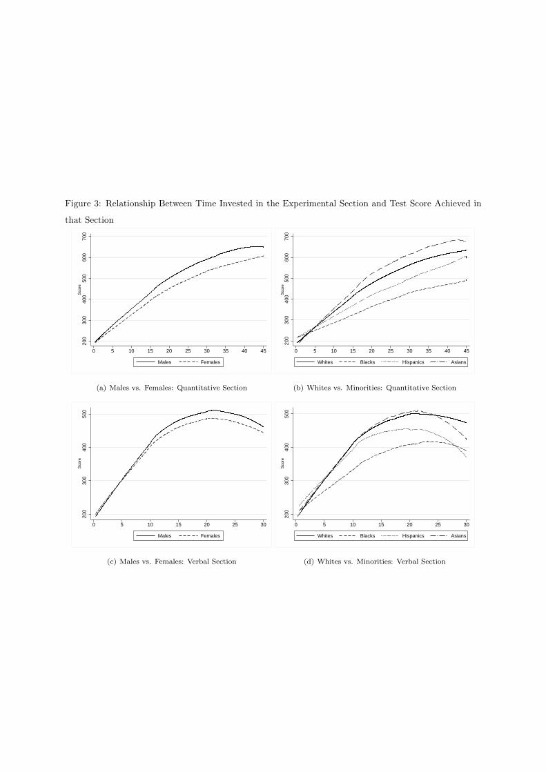
Figure 3: Relationship Between Time Invested in the Experimental Section and Test Score Achieved in
that Section
200
300
400
500
600
700
Sco
re
0 5 10 15 20 25 30 35 40 45
Males Females
(a) Males vs. Females: Quantitative Section
200
300
400
500
600
700
Sco
re
0 5 10 15 20 25 30 35 40 45
Whites Blacks Hispanics Asians
(b) Whites vs. Minorities: Quantitative Section
200
300
400
500
Sco
re
0 5 10 15 20 25 30
Males Females
(c) Males vs. Females: Verbal Section
200
300
400
500
Sco
re
0 5 10 15 20 25 30
Whites Blacks Hispanics Asians
(d) Whites vs. Minorities: Verbal Section
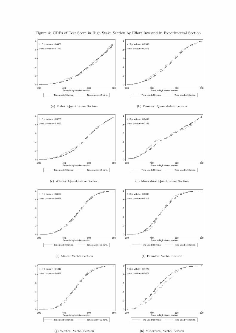
Figure 4: CDFs of Test Score in High Stake Section by Effort Invested in Experimental Section
K−S p−value= 0.6481
t−test p−value= 0.7747
0
.2
.4
.6
.8
1
200 400 600 800Score in high stakes section
Time used<10 mins. Time used>=10 mins.
(a) Males: Quantitative Section
K−S p−value= 0.6308
t−test p−value= 0.2879
0
.2
.4
.6
.8
1
200 400 600 800Score in high stakes section
Time used<10 mins. Time used>=10 mins.
(b) Females: Quantitative Section
K−S p−value= 0.3289
t−test p−value= 0.3092
0
.2
.4
.6
.8
1
200 400 600 800Score in high stakes section
Time used<10 mins. Time used>=10 mins.
(c) Whites: Quantitative Section
K−S p−value= 0.6496
t−test p−value= 0.7166
0
.2
.4
.6
.8
1
200 400 600 800Score in high stakes section
Time used<10 mins. Time used>=10 mins.
(d) Minorities: Quantitative Section
K−S p−value= 0.8177
t−test p−value= 0.6396
0
.2
.4
.6
.8
1
200 400 600 800Score in high stakes section
Time used<10 mins. Time used>=10 mins.
(e) Males: Verbal Section
K−S p−value= 0.0398
t−test p−value= 0.9316
0
.2
.4
.6
.8
1
200 400 600 800Score in high stakes section
Time used<10 mins. Time used>=10 mins.
(f) Females: Verbal Section
K−S p−value= 0.1810
t−test p−value= 0.4999
0
.2
.4
.6
.8
1
200 400 600 800Score in high stakes section
Time used<10 mins. Time used>=10 mins.
(g) Whites: Verbal Section
K−S p−value= 0.1723
t−test p−value= 0.0678
0
.2
.4
.6
.8
1
200 400 600 800Score in high stakes section
Time used<10 mins. Time used>=10 mins.
(h) Minorities: Verbal Section
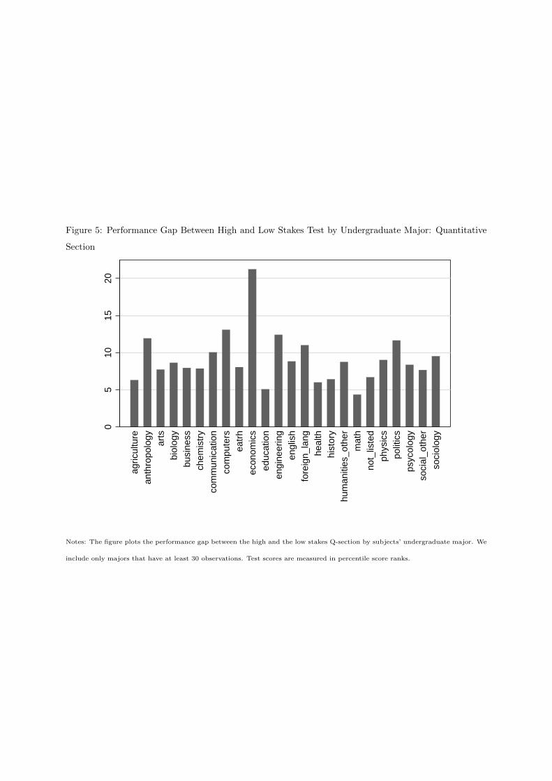
Figure 5: Performance Gap Between High and Low Stakes Test by Undergraduate Major: Quantitative
Section
05
1015
20
agric
ultu
rean
thro
polo
gyar
tsbi
olog
ybu
sine
ssch
emis
try
com
mun
icat
ion
com
pute
rsea
trh
econ
omic
sed
ucat
ion
engi
neer
ing
engl
ish
fore
ign_
lang
heal
thhi
stor
yhu
man
ities
_oth
erm
ath
not_
liste
dph
ysic
spo
litic
sps
ycol
ogy
soci
al_o
ther
soci
olog
y
Notes: The figure plots the performance gap between the high and the low stakes Q-section by subjects’ undergraduate major. We
include only majors that have at least 30 observations. Test scores are measured in percentile score ranks.
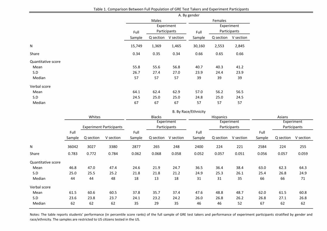
Q section V section Q section V section
N 15,749 1,369 1,465 30,160 2,553 2,845
Share 0.34 0.35 0.34 0.66 0.65 0.66
Quantitative score
Mean 55.8 55.6 56.8 40.7 40.3 41.2
S.D 26.7 27.4 27.0 23.9 24.4 23.9
Median 57 57 57 39 39 39
Verbal score
Mean 64.1 62.4 62.9 57.0 56.2 56.5
S.D 24.5 25.0 25.0 24.8 25.0 24.5
Median 67 67 67 57 57 57
Q section V section Q section V section Q section V section Q section V section
N 36042 3027 3380 2877 265 248 2400 224 221 2584 224 255
Share 0.783 0.772 0.784 0.062 0.068 0.058 0.052 0.057 0.051 0.056 0.057 0.059
Quantitative score
Mean 46.8 47.0 47.4 24.6 21.9 24.7 36.5 36.4 38.4 63.0 62.3 64.3
S.D 25.0 25.5 25.2 21.8 21.8 21.2 24.9 25.3 26.1 25.4 26.8 24.9
Median 44 44 48 18 13 18 31 31 35 66 66 71
Verbal score
Mean 61.5 60.6 60.5 37.8 35.7 37.4 47.6 48.8 48.7 62.0 61.5 60.8
S.D 23.6 23.8 23.7 24.1 23.2 24.2 26.0 26.8 26.2 26.8 27.1 26.8
Median 62 62 62 35 29 35 46 46 52 67 62 62
Notes: The table reports students' performance (in percentile score ranks) of the full sample of GRE test takers and performance of experiment participants stratified by gender and
race/ethnicity. The samples are restricted to US citizens tested in the US.
FemalesMales
Whites Blacks Hispanics
Table 1. Comparison Between Full Population of GRE Test Takers and Experiment Participants
A. By gender
Experiment
Participants
Full
Sample
Experiment
Participants
Full
Sample
Experiment Participants
Full
Sample
Experiment
Participants
Full
Sample
Asians
B. By Race/Ethnicity
Experiment
ParticipantsFull
Sample
Full
Sample
Experiment
Participants
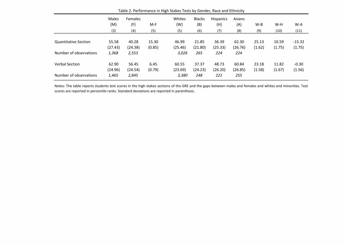
Males
(M)
Females
(F) M‐F
Whites
(W)
Blacks
(B)
Hispanics
(H)
Asians
(A) W‐B W‐H W‐A
(3) (4) (5) (5) (6) (7) (8) (9) (10) (11)
Quantitative Section 55.58 40.28 15.30 46.99 21.85 36.39 62.30 25.13 10.59 ‐15.32
(27.43) (24.38) (0.85) (25.46) (21.80) (25.33) (26.76) (1.62) (1.75) (1.75)
Number of observations 1,368 2,553 3,026 265 224 224
Verbal Section 62.90 56.45 6.45 60.55 37.37 48.73 60.84 23.18 11.82 ‐0.30
(24.96) (24.54) (0.79) (23.69) (24.23) (26.20) (26.85) (1.58) (1.67) (1.56)
Number of observations 1,465 2,845 3,380 248 221 255
Table 2. Performance in High Stakes Tests by Gender, Race and Ethnicity
Notes: The table reports students test scores in the high stakes sections of the GRE and the gaps between males and females and whites and minorities. Test
scores are reported in percentile ranks. Standard deviations are reported in parenthesis.
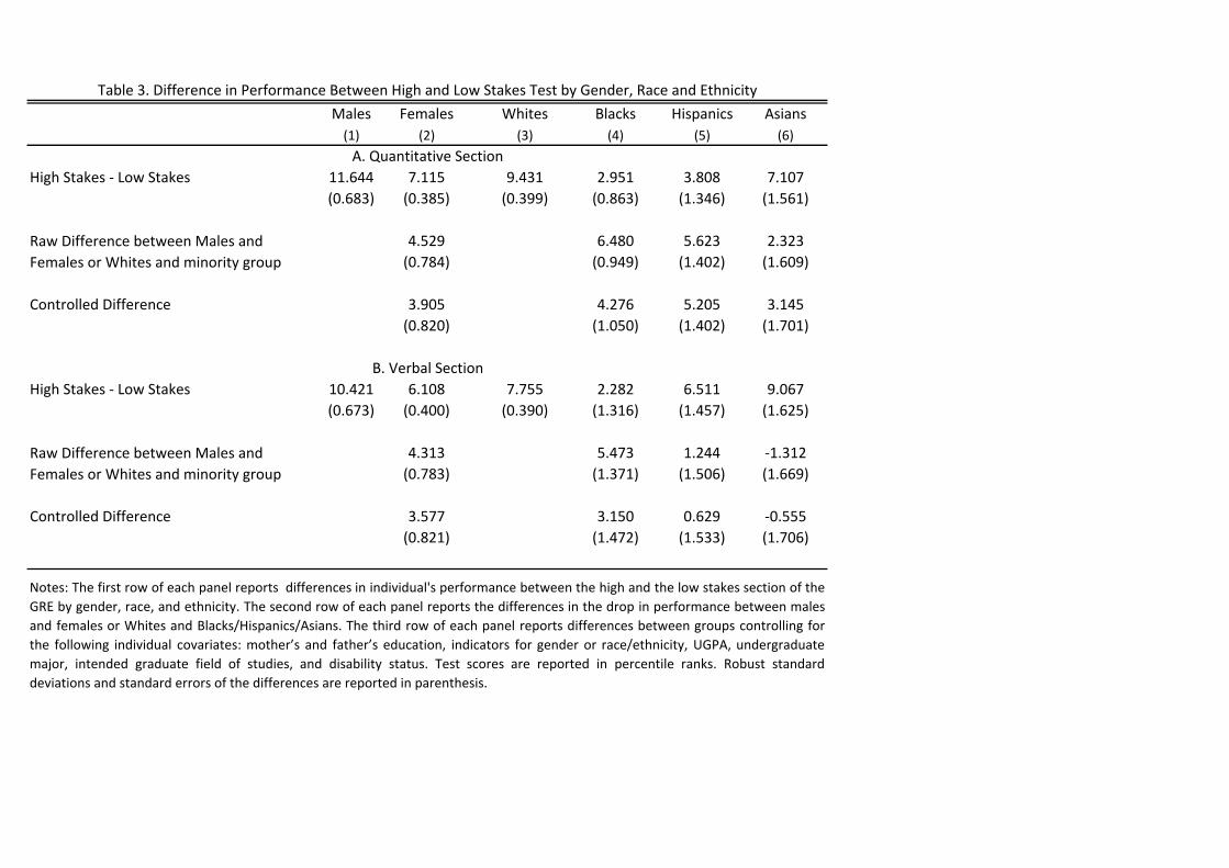
Males Females Whites Blacks Hispanics Asians
(1) (2) (3) (4) (5) (6)
High Stakes ‐ Low Stakes 11.644 7.115 9.431 2.951 3.808 7.107
(0.683) (0.385) (0.399) (0.863) (1.346) (1.561)
4.529 6.480 5.623 2.323
(0.784) (0.949) (1.402) (1.609)
Controlled Difference 3.905 4.276 5.205 3.145
(0.820) (1.050) (1.402) (1.701)
High Stakes ‐ Low Stakes 10.421 6.108 7.755 2.282 6.511 9.067
(0.673) (0.400) (0.390) (1.316) (1.457) (1.625)
4.313 5.473 1.244 ‐1.312
(0.783) (1.371) (1.506) (1.669)
Controlled Difference 3.577 3.150 0.629 ‐0.555
(0.821) (1.472) (1.533) (1.706)
A. Quantitative Section
B. Verbal Section
Raw Difference between Males and
Females or Whites and minority group
Table 3. Difference in Performance Between High and Low Stakes Test by Gender, Race and Ethnicity
Notes: The first row of each panel reports differences in individual's performance between the high and the low stakes section of the
GRE by gender, race, and ethnicity. The second row of each panel reports the differences in the drop in performance between males
and females or Whites and Blacks/Hispanics/Asians. The third row of each panel reports differences between groups controlling for
the following individual covariates: mother’s and father’s education, indicators for gender or race/ethnicity, UGPA, undergraduate
major, intended graduate field of studies, and disability status. Test scores are reported in percentile ranks. Robust standard
deviations and standard errors of the differences are reported in parenthesis.
Raw Difference between Males and
Females or Whites and minority group
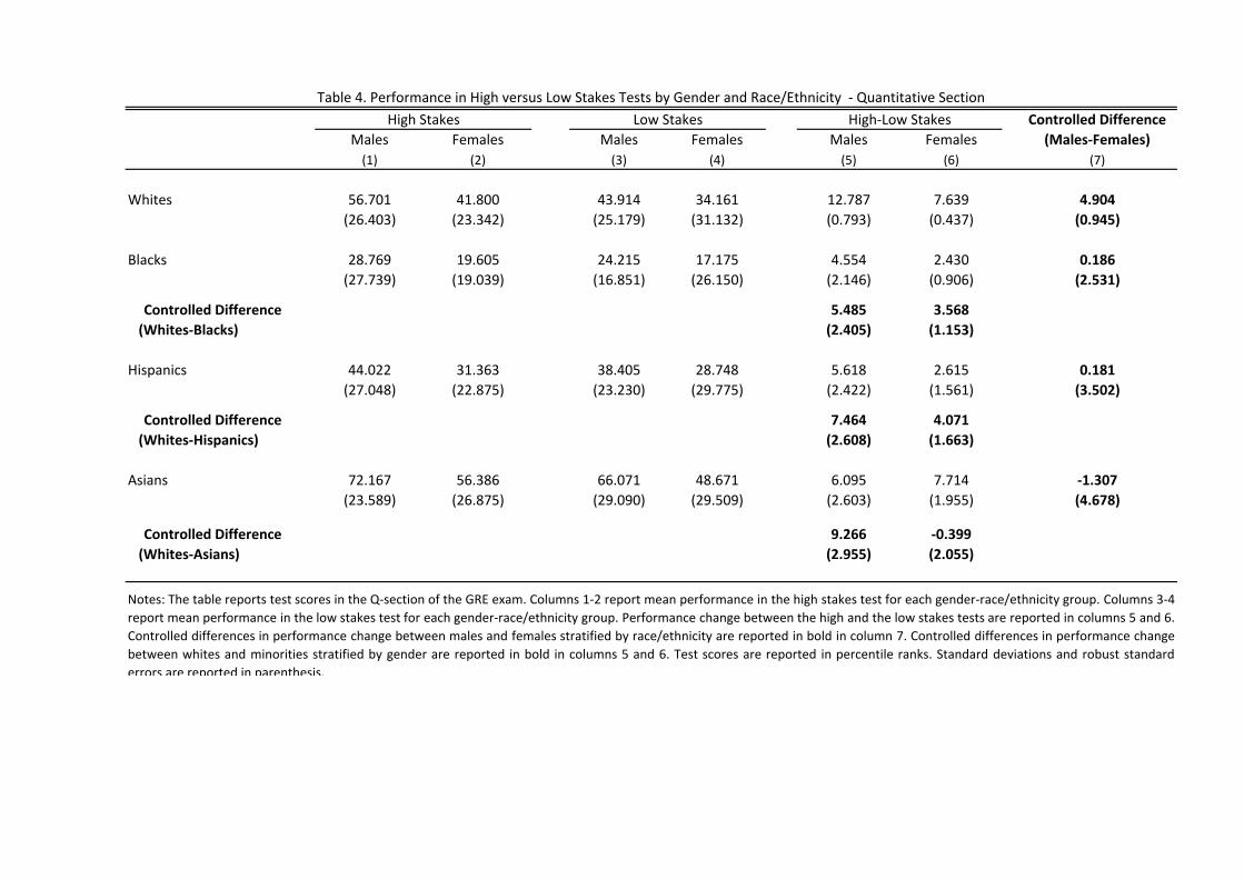
Controlled Difference
Males Females Males Females Males Females (Males‐Females)
(1) (2) (3) (4) (5) (6) (7)
Whites 56.701 41.800 43.914 34.161 12.787 7.639 4.904
(26.403) (23.342) (25.179) (31.132) (0.793) (0.437) (0.945)
Blacks 28.769 19.605 24.215 17.175 4.554 2.430 0.186
(27.739) (19.039) (16.851) (26.150) (2.146) (0.906) (2.531)
Controlled Difference 5.485 3.568
(Whites‐Blacks) (2.405) (1.153)
Hispanics 44.022 31.363 38.405 28.748 5.618 2.615 0.181
(27.048) (22.875) (23.230) (29.775) (2.422) (1.561) (3.502)
Controlled Difference 7.464 4.071
(Whites‐Hispanics) (2.608) (1.663)
Asians 72.167 56.386 66.071 48.671 6.095 7.714 ‐1.307
(23.589) (26.875) (29.090) (29.509) (2.603) (1.955) (4.678)
Controlled Difference 9.266 ‐0.399
(Whites‐Asians) (2.955) (2.055)
Table 4. Performance in High versus Low Stakes Tests by Gender and Race/Ethnicity ‐ Quantitative Section
High‐Low StakesHigh Stakes Low Stakes
Notes: The table reports test scores in the Q‐section of the GRE exam. Columns 1‐2 report mean performance in the high stakes test for each gender‐race/ethnicity group. Columns 3‐4
report mean performance in the low stakes test for each gender‐race/ethnicity group. Performance change between the high and the low stakes tests are reported in columns 5 and 6.
Controlled differences in performance change between males and females stratified by race/ethnicity are reported in bold in column 7. Controlled differences in performance change
between whites and minorities stratified by gender are reported in bold in columns 5 and 6. Test scores are reported in percentile ranks. Standard deviations and robust standard
errors are reported in parenthesis.
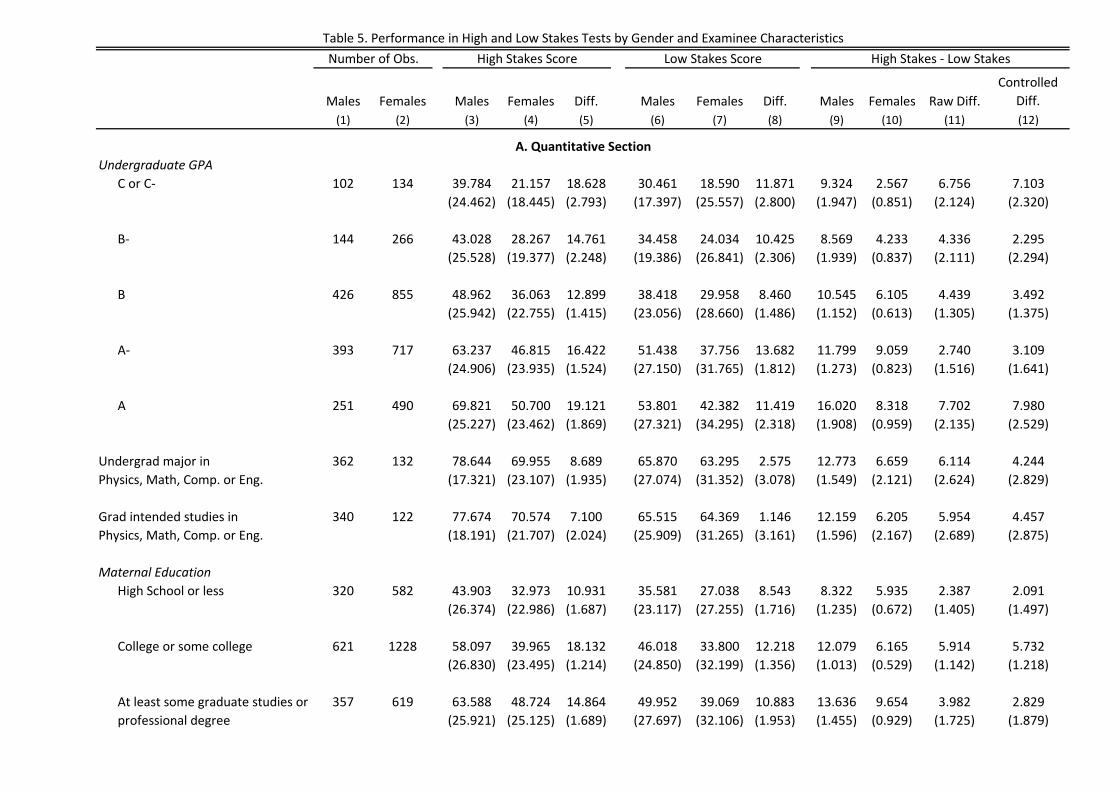
Males Females Males Females Diff. Males Females Diff. Males Females Raw Diff.
Controlled
Diff.
(1) (2) (3) (4) (5) (6) (7) (8) (9) (10) (11) (12)
Undergraduate GPA
C or C‐ 102 134 39.784 21.157 18.628 30.461 18.590 11.871 9.324 2.567 6.756 7.103
(24.462) (18.445) (2.793) (17.397) (25.557) (2.800) (1.947) (0.851) (2.124) (2.320)
B‐ 144 266 43.028 28.267 14.761 34.458 24.034 10.425 8.569 4.233 4.336 2.295
(25.528) (19.377) (2.248) (19.386) (26.841) (2.306) (1.939) (0.837) (2.111) (2.294)
B 426 855 48.962 36.063 12.899 38.418 29.958 8.460 10.545 6.105 4.439 3.492
(25.942) (22.755) (1.415) (23.056) (28.660) (1.486) (1.152) (0.613) (1.305) (1.375)
A‐ 393 717 63.237 46.815 16.422 51.438 37.756 13.682 11.799 9.059 2.740 3.109
(24.906) (23.935) (1.524) (27.150) (31.765) (1.812) (1.273) (0.823) (1.516) (1.641)
A 251 490 69.821 50.700 19.121 53.801 42.382 11.419 16.020 8.318 7.702 7.980
(25.227) (23.462) (1.869) (27.321) (34.295) (2.318) (1.908) (0.959) (2.135) (2.529)
Undergrad major in 362 132 78.644 69.955 8.689 65.870 63.295 2.575 12.773 6.659 6.114 4.244
Physics, Math, Comp. or Eng. (17.321) (23.107) (1.935) (27.074) (31.352) (3.078) (1.549) (2.121) (2.624) (2.829)
Grad intended studies in 340 122 77.674 70.574 7.100 65.515 64.369 1.146 12.159 6.205 5.954 4.457
Physics, Math, Comp. or Eng. (18.191) (21.707) (2.024) (25.909) (31.265) (3.161) (1.596) (2.167) (2.689) (2.875)
Maternal Education
High School or less 320 582 43.903 32.973 10.931 35.581 27.038 8.543 8.322 5.935 2.387 2.091
(26.374) (22.986) (1.687) (23.117) (27.255) (1.716) (1.235) (0.672) (1.405) (1.497)
College or some college 621 1228 58.097 39.965 18.132 46.018 33.800 12.218 12.079 6.165 5.914 5.732
(26.830) (23.495) (1.214) (24.850) (32.199) (1.356) (1.013) (0.529) (1.142) (1.218)
357 619 63.588 48.724 14.864 49.952 39.069 10.883 13.636 9.654 3.982 2.829
(25.921) (25.125) (1.689) (27.697) (32.106) (1.953) (1.455) (0.929) (1.725) (1.879)
At least some graduate studies or
professional degree
Table 5. Performance in High and Low Stakes Tests by Gender and Examinee Characteristics
High Stakes Score Low Stakes Score High Stakes ‐ Low Stakes
A. Quantitative Section
Number of Obs.
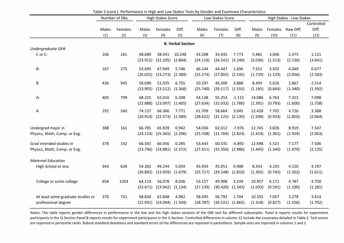
Males Females Males Females Diff. Males Females Diff. Males Females Raw Diff.
Controlled
Diff.
(1) (2) (3) (4) (5) (6) (7) (8) (9) (10) (11) (12)
Undergraduate GPA
C or C‐ 106 161 48.689 38.441 10.248 43.208 35.435 7.773 5.481 3.006 2.475 1.121
(23.915) (22.205) (2.864) (24.116) (26.541) (3.140) (2.036) (1.513) (2.536) (3.641)
B‐ 167 275 53.695 47.949 5.746 46.144 44.447 1.696 7.551 3.502 4.049 0.677
(26.025) (23.273) (2.389) (25.274) (27.002) (2.545) (1.719) (1.129) (2.056) (2.583)
B 436 945 58.690 51.935 6.755 50.197 46.309 3.888 8.493 5.626 2.867 2.514
(23.905) (23.512) (1.368) (25.740) (29.117) (1.555) (1.165) (0.664) (1.340) (1.392)
A‐ 405 799 68.225 62.016 6.208 54.138 55.253 ‐1.115 14.086 6.763 7.323 7.098
(22.888) (23.097) (1.405) (27.634) (32.032) (1.780) (1.391) (0.793) (1.600) (1.738)
A 292 560 74.137 66.366 7.771 61.709 58.664 3.045 12.428 7.702 4.726 3.388
(20.914) (22.573) (1.589) (28.622) (31.125) (2.130) (1.598) (0.933) (1.850) (2.064)
Undergrad major in 388 161 66.781 65.839 0.942 54.036 62.012 ‐7.976 12.745 3.826 8.919 7.547
Physics, Math, Comp. or Eng. (24.124) (25.365) (2.296) (25.708) (31.769) (2.824) (1.424) (1.301) (1.929) (2.063)
Grad intended studies in 378 142 66.341 66.056 0.285 53.643 60.535 ‐6.892 12.698 5.521 7.177 7.506
Physics, Math, Comp. or Eng. (23.796) (24.881) (2.372) (27.411) (31.356) (2.986) (1.445) (1.340) (1.970) (2.135)
Maternal Education
High School or less 344 628 54.302 49.244 5.059 45.959 45.051 0.908 8.343 4.193 4.150 4.197
(26.892) (23.959) (1.679) (25.717) (29.148) (1.810) (1.305) (0.745) (1.502) (1.611)
College or some college 658 1354 64.114 56.078 8.036 53.157 49.908 3.249 10.957 6.171 4.787 4.750
(23.671) (23.942) (1.134) (27.139) (30.420) (1.343) (1.033) (0.591) (1.190) (1.281)
376 731 68.830 63.848 4.982 58.495 56.791 1.704 10.335 7.057 3.278 3.614
(22.931) (24.094) (1.504) (28.787) (30.521) (1.865) (1.318) (0.827) (1.556) (1.702)
Notes: The table reports gender differences in performance in the low and the high stakes sections of the GRE test for different subsamples. Panel A reports results for experiment
participants in the Q‐Section Panel B reports results for experiment participants in the V‐Section. Controlled differences in column 12 include the covariates detailed in Table 2. Test scores
are reported in percentile ranks. Robust standard deviations and standard errors of the differences are reported in parenthesis. Sample sizes are reported in columns 1 and 2.
Table 5 (cont.). Performance in High and Low Stakes Tests by Gender and Examinee Characteristics
High Stakes Score Low Stakes Score High Stakes ‐ Low Stakes
At least some graduate studies or
professional degree
B. Verbal Section
Number of Obs.
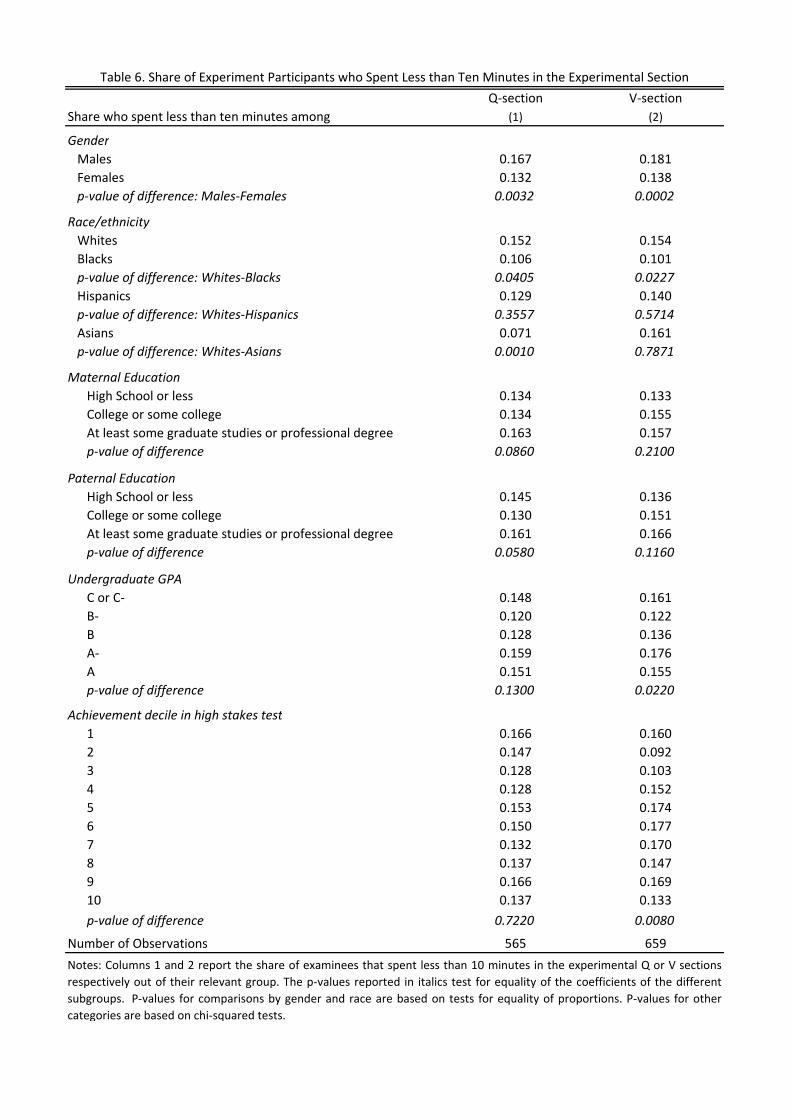
Q‐section V‐section
Share who spent less than ten minutes among (1) (2)
Gender
Males 0.167 0.181
Females 0.132 0.138
p‐value of difference: Males‐Females 0.0032 0.0002
Race/ethnicity
Whites 0.152 0.154
Blacks 0.106 0.101
p‐value of difference: Whites‐Blacks 0.0405 0.0227
Hispanics 0.129 0.140
p‐value of difference: Whites‐Hispanics 0.3557 0.5714
Asians 0.071 0.161
p‐value of difference: Whites‐Asians 0.0010 0.7871
Maternal Education
High School or less 0.134 0.133
College or some college 0.134 0.155
At least some graduate studies or professional degree 0.163 0.157
p‐value of difference 0.0860 0.2100
Paternal Education
High School or less 0.145 0.136
College or some college 0.130 0.151
At least some graduate studies or professional degree 0.161 0.166
p‐value of difference 0.0580 0.1160
Undergraduate GPA
C or C‐ 0.148 0.161
B‐ 0.120 0.122
B 0.128 0.136
A‐ 0.159 0.176
A 0.151 0.155
p‐value of difference 0.1300 0.0220
Achievement decile in high stakes test
1 0.166 0.160
2 0.147 0.092
3 0.128 0.103
4 0.128 0.152
5 0.153 0.174
6 0.150 0.177
7 0.132 0.170
8 0.137 0.147
9 0.166 0.169
10 0.137 0.133
p‐value of difference 0.7220 0.0080
Number of Observations 565 659
Notes: Columns 1 and 2 report the share of examinees that spent less than 10 minutes in the experimental Q or V sections
respectively out of their relevant group. The p‐values reported in italics test for equality of the coefficients of the different
subgroups. P‐values for comparisons by gender and race are based on tests for equality of proportions. P‐values for other
categories are based on chi‐squared tests.
Table 6. Share of Experiment Participants who Spent Less than Ten Minutes in the Experimental Section
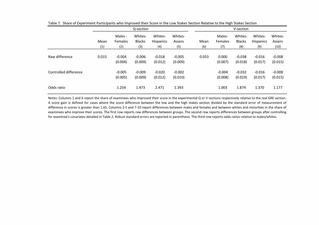
Table 7. Share of Experiment Participants who Improved their Score in the Low Stakes Section Relative to the High Stakes Section
Mean
Males ‐
Females
Whites‐
Blacks
Whites‐
Hispanics
Whites‐
Asians Mean
Males‐
Females
Whites‐
Blacks
Whites‐
Hispanics
Whites‐
Asians
(1) (2) (3) (4) (5) (6) (7) (8) (9) (10)
Raw difference 0.015 ‐0.004 ‐0.006 ‐0.018 ‐0.005 0.053 0.000 ‐0.038 ‐0.016 ‐0.008
(0.004) (0.009) (0.012) (0.009) (0.007) (0.018) (0.017) (0.015)
Controlled difference ‐0.005 ‐0.009 ‐0.020 ‐0.002 ‐0.004 ‐0.032 ‐0.016 ‐0.008
(0.005) (0.009) (0.012) (0.010) (0.008) (0.019) (0.017) (0.015)
Odds ratio 1.254 1.473 2.471 1.393 1.003 1.874 1.370 1.177
Notes: Columns 1 and 6 report the share of examinees who improved their score in the experimental Q or V sections respectively relative to the real GRE section.
A score gain is defined for cases where the score difference between the low and the high stakes section divided by the standard error of measurement of
difference in scores is greater than 1.65. Columns 2‐5 and 7‐10 report differences between males and females and between whites and minorities in the share of
examinees who improve their scores. The first row reports raw differences between groups. The second row reports differences between groups after controlling
for examinee's covariates detailed in Table 2. Robust standard errors are reported in parenthesis. The third row reports odds ratios relative to males/whites.
Q‐section V‐section
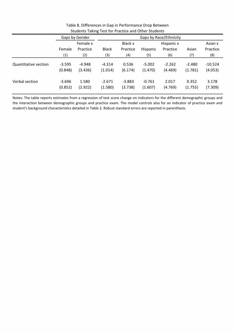
Female
Female x
Practice Black
Black x
Practice Hispanic
Hispanic x
Practice Asian
Asian x
Practice
(1) (2) (3) (4) (5) (6) (7) (8)
Quantitative section ‐3.595 ‐4.948 ‐4.314 0.536 ‐5.002 ‐2.262 ‐2.480 ‐10.524
(0.848) (3.436) (1.014) (6.174) (1.470) (4.469) (1.781) (4.053)
Verbal section ‐3.696 1.580 ‐2.671 ‐3.883 ‐0.761 2.017 0.352 3.178
(0.852) (2.922) (1.580) (3.738) (1.607) (4.769) (1.755) (7.309)
Gaps by Gender Gaps by Race/Ethnicity
Table 8. Differences in Gap in Performance Drop Between
Students Taking Test for Practice and Other Students
Notes: The table reports estimates from a regression of test score change on indicators for the different demographic groups and
the interaction between demographic groups and practice exam. The model controls also for an indicator of practice exam and
student's background characteristics detailed in Table 2. Robust standard errors are reported in parenthesis.
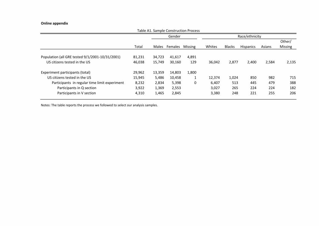
Online appendix
Total Males Females Missing Whites Blacks Hispanics Asians
Other/
Missing
Population (all GRE tested 9/1/2001‐10/31/2001) 81,231 34,723 41,617 4,891
US citizens tested in the US 46,038 15,749 30,160 129 36,042 2,877 2,400 2,584 2,135
Experiment participants (total) 29,962 13,359 14,803 1,800
US citizens tested in the US 15,945 5,486 10,458 1 12,374 1,024 850 982 715
Participants in regular time limit experiment 8,232 2,834 5,398 0 6,407 513 445 479 388
Participants in Q section 3,922 1,369 2,553 3,027 265 224 224 182
Participants in V section 4,310 1,465 2,845 3,380 248 221 255 206
Gender Race/ethnicity
Table A1. Sample Construction Process
Notes: The table reports the process we followed to select our analysis samples.
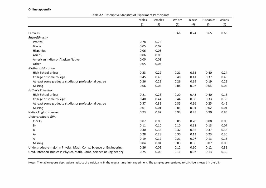
Online appendix
Males Females Whites Blacks Hispanics Asians
(1) (2) (3) (4) (5) (6)
Females 0.66 0.74 0.65 0.63
Race/Ethnicity
Whites 0.78 0.78
Blacks 0.05 0.07
Hispanics 0.06 0.05
Asians 0.06 0.06
American Indian or Alaskan Native 0.00 0.01
Other 0.05 0.04
Mother's Education
High School or less 0.23 0.22 0.21 0.33 0.40 0.24
College or some college 0.45 0.48 0.48 0.41 0.37 0.46
At least some graduate studies or professional degree 0.26 0.25 0.26 0.19 0.19 0.25
Missing 0.06 0.05 0.04 0.07 0.04 0.05
Father's Education
High School or less 0.21 0.23 0.20 0.43 0.40 0.15
College or some college 0.40 0.44 0.44 0.38 0.33 0.39
At least some graduate studies or professional degree 0.37 0.32 0.35 0.16 0.25 0.45
Missing 0.01 0.01 0.01 0.04 0.02 0.01
Native English speaker 0.93 0.92 0.93 0.95 0.90 0.86
Undergraduate GPA
C or C‐ 0.07 0.05 0.05 0.20 0.08 0.05
B‐ 0.11 0.10 0.10 0.18 0.13 0.07
B 0.30 0.33 0.32 0.36 0.37 0.36
A‐ 0.28 0.28 0.30 0.13 0.23 0.30
A 0.19 0.19 0.21 0.07 0.13 0.18
Missing 0.04 0.04 0.03 0.06 0.07 0.05
Undergraduate major in Physics, Math, Comp. Science or Engineering 0.26 0.05 0.12 0.10 0.12 0.31
Grad. intended studies in Physics, Math, Comp. Science or Engineering 0.25 0.05 0.11 0.07 0.13 0.30
Table A2. Descriptive Statistics of Experiment Participants
Notes: The table reports descriptive statistics of participants in the regular time limit experiment. The samples are restricted to US citizens tested in the US.
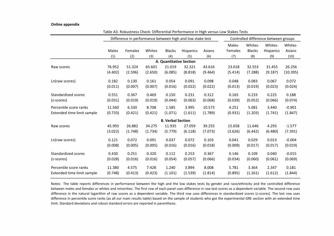
Online appendix
Males Females Whites Blacks Hispanics Asians
Males‐
Females
Whites‐
Blacks
Whites‐
Hispanics
Whites‐
Asians
(1) (2) (3) (4) (5) (6) (7) (8) (9) (10)
Raw scores 76.952 51.324 65.601 21.019 32.321 43.616 23.018 32.553 31.455 26.256
(4.402) (2.596) (2.650) (6.085) (8.818) (9.464) (5.414) (7.288) (9.187) (10.395)
Ln(raw scores) 0.182 0.130 0.161 0.054 0.091 0.098 0.048 0.083 0.067 0.072
(0.011) (0.007) (0.007) (0.016) (0.022) (0.022) (0.013) (0.019) (0.023) (0.024)
Standardized scores 0.551 0.367 0.469 0.150 0.231 0.312 0.165 0.233 0.225 0.188
(z‐scores) (0.031) (0.019) (0.019) (0.044) (0.063) (0.068) (0.039) (0.052) (0.066) (0.074)
Percentile score ranks 11.560 6.330 8.708 1.585 3.995 10.573 4.251 5.081 3.440 ‐0.901
Extended time limit sample (0.733) (0.421) (0.421) (1.071) (1.611) (1.789) (0.931) (1.203) (1.741) (1.847)
Raw scores 45.993 26.882 34.275 11.935 27.059 39.255 15.658 11.646 4.293 ‐1.577
(3.022) (1.748) (1.734) (5.779) (6.118) (7.073) (3.626) (6.442) (6.480) (7.391)
Ln(raw scores) 0.121 0.072 0.091 0.037 0.072 0.103 0.041 0.029 0.013 ‐0.004
(0.008) (0.005) (0.005) (0.016) (0.016) (0.018) (0.009) (0.017) (0.017) (0.019)
Standardized scores 0.430 0.251 0.320 0.112 0.253 0.367 0.146 0.109 0.040 ‐0.015
(z‐scores) (0.028) (0.016) (0.016) (0.054) (0.057) (0.066) (0.034) (0.060) (0.061) (0.069)
Percentile score ranks 11.380 4.575 7.428 1.240 3.894 8.008 5.781 3.364 2.347 0.181
Extended time limit sample (0.748) (0.413) (0.423) (1.101) (1.539) (1.814) (0.895) (1.261) (1.612) (1.844)
Notes: The table reports differences in performance between the high and the low stakes tests by gender and race/ethnicity and the controlled difference
between males and females or whites and minorities. The first row of each panel uses difference in raw test scores as a dependent variable. The second row uses
difference in the natural logarithm of raw scores as a dependent variable. The third row uses differences in standardized scores (z‐scores). The last row uses
difference in percentile score ranks (as all our main results table) based on the sample of students who got the experimental GRE section with an extended time
limit. Standard deviations and robust standard errors are reported in parenthesis.
Table A3. Robustness Check: Differential Performance in High versus Low Stakes Tests
Difference in performance between high and low stake test Controlled difference between groups
A. Quantitative Section
B. Verbal Section
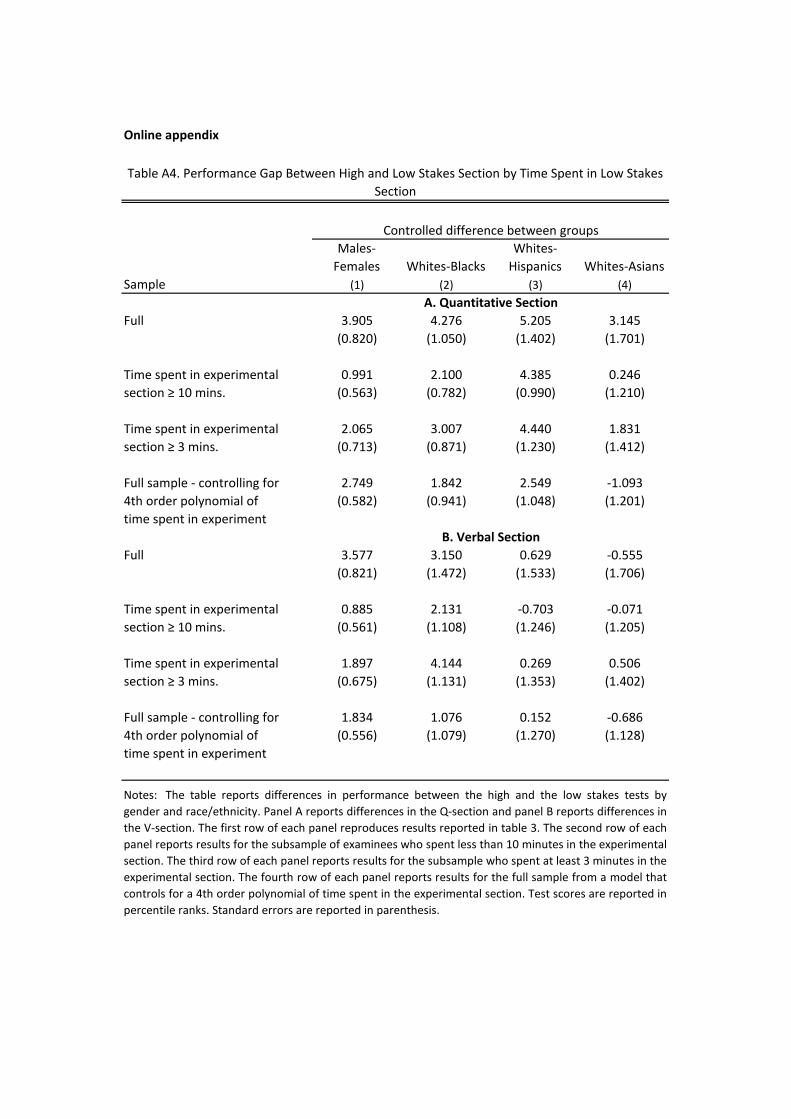
Online appendix
Males‐
Females Whites‐Blacks
Whites‐
Hispanics Whites‐Asians
Sample (1) (2) (3) (4)
Full 3.905 4.276 5.205 3.145
(0.820) (1.050) (1.402) (1.701)
0.991 2.100 4.385 0.246
(0.563) (0.782) (0.990) (1.210)
2.065 3.007 4.440 1.831
(0.713) (0.871) (1.230) (1.412)
Full sample ‐ controlling for 2.749 1.842 2.549 ‐1.093
4th order polynomial of (0.582) (0.941) (1.048) (1.201)
time spent in experiment
Full 3.577 3.150 0.629 ‐0.555
(0.821) (1.472) (1.533) (1.706)
0.885 2.131 ‐0.703 ‐0.071
(0.561) (1.108) (1.246) (1.205)
1.897 4.144 0.269 0.506
(0.675) (1.131) (1.353) (1.402)
Full sample ‐ controlling for 1.834 1.076 0.152 ‐0.686
4th order polynomial of (0.556) (1.079) (1.270) (1.128)
time spent in experiment
Notes: The table reports differences in performance between the high and the low stakes tests by
gender and race/ethnicity. Panel A reports differences in the Q‐section and panel B reports differences in
the V‐section. The first row of each panel reproduces results reported in table 3. The second row of each
panel reports results for the subsample of examinees who spent less than 10 minutes in the experimental
section. The third row of each panel reports results for the subsample who spent at least 3 minutes in the
experimental section. The fourth row of each panel reports results for the full sample from a model that
controls for a 4th order polynomial of time spent in the experimental section. Test scores are reported in
percentile ranks. Standard errors are reported in parenthesis.
Time spent in experimental
section ≥ 10 mins.
Time spent in experimental
section ≥ 10 mins.
Table A4. Performance Gap Between High and Low Stakes Section by Time Spent in Low Stakes
Section
Controlled difference between groups
Time spent in experimental
section ≥ 3 mins.
Time spent in experimental
section ≥ 3 mins.
B. Verbal Section
A. Quantitative Section
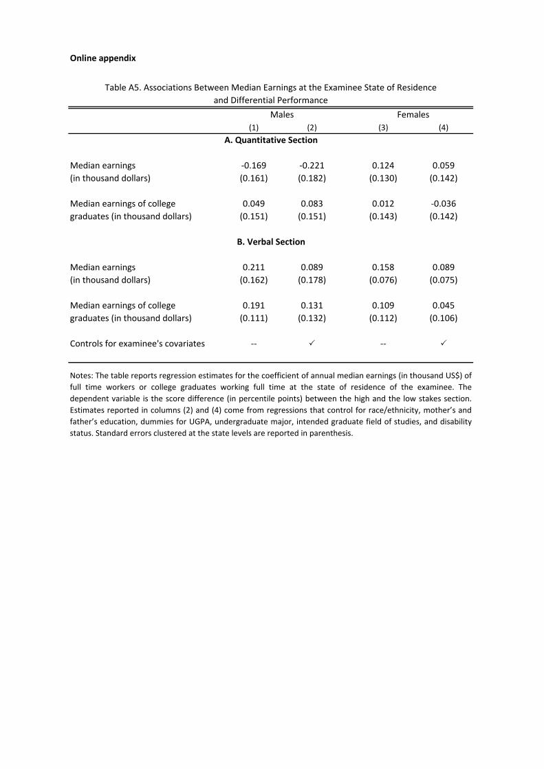
Online appendix
(1) (2) (3) (4)
Median earnings ‐0.169 ‐0.221 0.124 0.059
(in thousand dollars) (0.161) (0.182) (0.130) (0.142)
Median earnings of college 0.049 0.083 0.012 ‐0.036
graduates (in thousand dollars) (0.151) (0.151) (0.143) (0.142)
Median earnings 0.211 0.089 0.158 0.089
(in thousand dollars) (0.162) (0.178) (0.076) (0.075)
Median earnings of college 0.191 0.131 0.109 0.045
graduates (in thousand dollars) (0.111) (0.132) (0.112) (0.106)
Controls for examinee's covariates ‐‐ ‐‐
Table A5. Associations Between Median Earnings at the Examinee State of Residence
and Differential Performance
Notes: The table reports regression estimates for the coefficient of annual median earnings (in thousand US$) of
full time workers or college graduates working full time at the state of residence of the examinee. The
dependent variable is the score difference (in percentile points) between the high and the low stakes section.
Estimates reported in columns (2) and (4) come from regressions that control for race/ethnicity, mother’s and
father’s education, dummies for UGPA, undergraduate major, intended graduate field of studies, and disability
status. Standard errors clustered at the state levels are reported in parenthesis.
B. Verbal Section
Females
A. Quantitative Section
Males
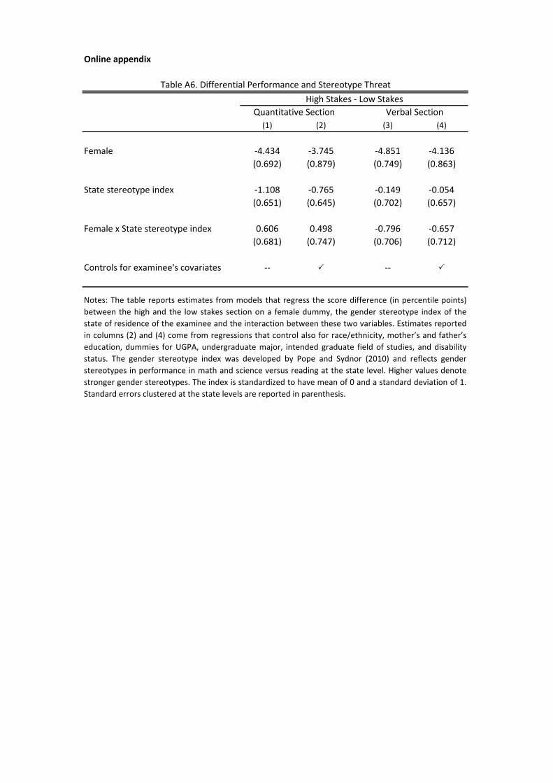
Online appendix
(1) (2) (3) (4)
Female ‐4.434 ‐3.745 ‐4.851 ‐4.136
(0.692) (0.879) (0.749) (0.863)
State stereotype index ‐1.108 ‐0.765 ‐0.149 ‐0.054
(0.651) (0.645) (0.702) (0.657)
Female x State stereotype index 0.606 0.498 ‐0.796 ‐0.657
(0.681) (0.747) (0.706) (0.712)
Controls for examinee's covariates ‐‐ ‐‐
Table A6. Differential Performance and Stereotype Threat
High Stakes ‐ Low Stakes
Quantitative Section Verbal Section
Notes: The table reports estimates from models that regress the score difference (in percentile points)
between the high and the low stakes section on a female dummy, the gender stereotype index of the
state of residence of the examinee and the interaction between these two variables. Estimates reported
in columns (2) and (4) come from regressions that control also for race/ethnicity, mother’s and father’s
education, dummies for UGPA, undergraduate major, intended graduate field of studies, and disability
status. The gender stereotype index was developed by Pope and Sydnor (2010) and reflects gender
stereotypes in performance in math and science versus reading at the state level. Higher values denote
stronger gender stereotypes. The index is standardized to have mean of 0 and a standard deviation of 1.
Standard errors clustered at the state levels are reported in parenthesis.
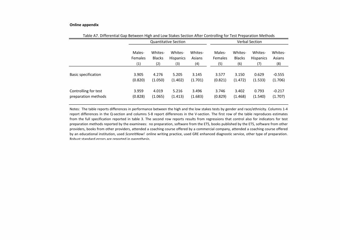
Online appendix
Males‐
Females
Whites‐
Blacks
Whites‐
Hispanics
Whites‐
Asians
Males‐
Females
Whites‐
Blacks
Whites‐
Hispanics
Whites‐
Asians
(1) (2) (3) (4) (5) (6) (7) (8)
Basic specification 3.905 4.276 5.205 3.145 3.577 3.150 0.629 ‐0.555
(0.820) (1.050) (1.402) (1.701) (0.821) (1.472) (1.533) (1.706)
3.959 4.019 5.216 3.496 3.746 3.402 0.793 ‐0.217
(0.828) (1.065) (1.413) (1.683) (0.829) (1.468) (1.540) (1.707)
Table A7. Differential Gap Between High and Low Stakes Section After Controlling for Test Preparation Methods
Verbal Section
Notes: The table reports differences in performance between the high and the low stakes tests by gender and race/ethnicity. Columns 1‐4
report differences in the Q‐section and columns 5‐8 report differences in the V‐section. The first row of the table reproduces estimates
from the full specification reported in table 3. The second row reports results from regressions that control also for indicators for test
preparation methods reported by the examinees: no preparation, software from the ETS, books published by the ETS, software from other
providers, books from other providers, attended a coaching course offered by a commercial company, attended a coaching course offered
by an educational institution, used ScoreItNow! online writing practice, used GRE enhanced diagnostic service, other type of preparation.
Robust standard errors are reported in parenthesis.
Quantitative Section
Controlling for test
preparation methods
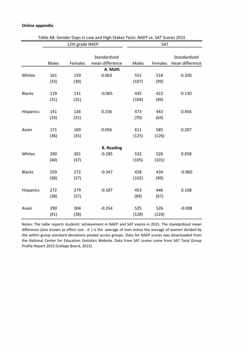
Online appendix
Males Females
Standardized
mean difference Males Females
Standardized
mean difference
Whites 161 159 0.063 551 518 0.320
(33) (30) (107) (99)
Blacks 129 131 ‐0.065 435 422 0.130
(31) (31) (104) (96)
Hispanics 141 136 0.156 473 443 0.456
(33) (31) (70) (64)
Asian 171 169 0.056 611 585 0.207
(36) (35) (125) (126)
Whites 290 301 ‐0.285 532 526 0.058
(40) (37) (105) (101)
Blacks 259 272 ‐0.347 428 434 ‐0.060
(38) (37) (102) (99)
Hispanics 272 279 ‐0.187 453 446 0.108
(38) (37) (69) (67)
Asian 290 304 ‐0.354 525 526 ‐0.008
(41) (38) (128) (124)
Table A8. Gender Gaps in Low and High Stakes Tests: NAEP vs. SAT Scores 2015
Notes: The table reports students' achievement in NAEP and SAT exams in 2015. The standardized mean
difference (also known as effect size ‐ d ) is the average of men minus the average of women divided by
the within group standard deviations pooled across groups. Data for NAEP scores was downloaded from
the National Center for Education Statistics Website. Data from SAT scores come from SAT Total Group
Profile Report 2015 (College Board, 2015).
12th grade NAEP
A. Math
B. Reading
SAT