Embed Size (px)
Citation preview
The Economic Journal, 129 (October), 2916–2948 DOI: 10.1093/ej/uez015 C© 2019 Royal Economic Society. Published by Oxford University Press. All rights
reserved. For permissions please contact [email protected].
Advance Access Publication Date: 16 May 2019
DIFFERENTIAL PERFORMANCE IN HIGH VERSUS LOW
STAKES TESTS: EVIDENCE FROM THE GRE TEST*
Analia Schlosser, Zvika Neeman and Yigal Attali
We study how different demographic groups respond to incentives by comparing their performance in ‘high’and ‘low’ stakes situations. The high stakes situation is the Graduate Record Examination (GRE), and thelow stakes situation is a voluntary experimental section of the GRE. We find that males exhibit a larger dropin performance between the high and low stakes examinations than females, and that whites exhibit a largerdrop in performance than minorities. Differences between high and low stakes tests are partly explained bythe fact that males and whites exert lower effort in low stakes tests compared with females and minorities.
Recently, there has been much interest in the question of whether different demographic groupsrespond differently to incentives and competitive pressure. Interest in this subject stems fromattempts to explain gender, racial and ethnic differences in human capital accumulation and labourmarket performance, and is further motivated by the increased use of aptitude tests for collegeadmissions and job screening and by the growing use of standardised tests for the assessment ofstudents’ learning. While it is clear that motivation affects performance, less attention has beengiven to demographic group differences in response to performance-based incentives.
In this paper, we examine whether individuals respond differently to incentives by analysingtheir performance in the Graduate Record Examination (GRE) General Test.1 We examine differ-ences in response to incentives between males and females as well as differences among whites,Asians, blacks and Hispanics. Specifically, we compare performance in the GRE examinationin ‘high’ and ‘low’ stakes situations. The high stakes situation is the real GRE examination andthe low stakes situation is a voluntary experimental section of the GRE test that examinees wereinvited to take part in immediately after they finished the real GRE examination.
A unique characteristic of our study is that we observe individuals’ performance in a ‘real’ highstakes situation that has important implications for success in life and that is administered to avery large and easily characterisable population, namely the population of applicants to graduateprograms in arts and sciences in the United States. This feature distinguishes our work frommost of the literature, which is usually based on controlled experiments that require individualsto perform tasks that might not bear directly on their everyday life, that manipulate the stakes,
* Corresponding author: Analia Schlosser, Berglas School of Economics, Tel Aviv University, Ramat Aviv, Tel Aviv69978, Israel. Email: [email protected].
This paper was received on 6 March 2017 and accepted on 20 August 2018. The Editor was Kjell Salvanes.
We are grateful for comments received at the SOLE meeting, ‘Discrimination at Work’ and ‘Frontiers in Economics ofEducation’ workshops, and seminar participants at the Federal Reserve Bank of Chicago, CESifo, Copenhagen BusinessSchool, Norwegian Business School, University of Zurich, Bar Ilan University, Ben Gurion University, and Universityof Haifa. This research was supported by the Israeli Science Foundation(grant No. 1035/12).
1 The GRE test is a commercially run psychometric examination that is part of the requirements for admission intomost graduate programs in arts and sciences in the United States and other English-speaking countries. Each year, morethan 600,000 prospective graduate school applicants from approximately 230 countries take the GRE General Test. Theexam measures verbal reasoning, quantitative reasoning, critical thinking and analytical writing skills that have beenacquired over a long period of time and that are not related to any specific field of study. For more information, see theETS website: http://www.ets.org/gre/general/about/.
[ 2916 ]
Dow
nloaded from https://academ
ic.oup.com/ej/article/129/623/2916/5490319 by Tel Aviv U
niversity user on 09 August 2020
2019] performance in high vs. low stakes tests 2917
degree of competitiveness, or incentive levels in somewhat artificial ways, and where stakes arenot as high as in real-life important events. A second distinctive feature of our research is that weare able to observe the performance of the same individual in high and low stakes situations thatinvolve the exact same task. A third unique feature of our study is the availability of rich dataon individuals’ characteristics that includes information on family background, college majorand academic performance, and intended graduate field of studies. These comprehensive dataallow us to compare individuals of similar academic and family backgrounds and to examine thepersistence of our results across different subgroups. A fourth important advantage of our studyis that we are able to observe the selection of individuals into the experiment and examine theextent of differential selection within and across groups. Notably, we do not find any evidenceof differential selection into the experiment, neither according to gender, race or ethnicity, noraccording to individual’s scores in the ‘real’ GRE.
Our results show that males exhibit a larger difference in performance between the high andlow stakes GRE than females, and that whites exhibit a larger difference in performance betweenthe high and low stakes GRE test than Asians, blacks and Hispanics. A direct consequence ofour findings is that test score gaps between males and females or between whites and blacksor Hispanics are larger in a high stakes test than in a low stakes test, while the test score gapbetween Asians and whites is larger in the low stakes test. Specifically, while males outperformfemales in the high stakes quantitative section of the GRE by 0.55 standard deviations (SD), thegender gap in performance in the low stakes section is only 0.30 SD. Similarly, males’ advantagein the high stakes verbal section is 0.26 SD, while the gender gap in the low stakes section isonly 0.07 SD. Whites outperform blacks and Hispanics in the high stakes quantitative sectionby 1.1 SD and 0.42 SD, respectively, but the gaps are significantly reduced in the low stakessection, to 0.63 and 0.14 SD. This pattern is reversed for Asians because they outperform whitesby 0.51 SD in the high stakes quantitative section, so that the gap increases to 0.55 SD in the lowstakes section. These group differences in performance between high and low stakes tests appearacross all undergraduate GPA levels, family backgrounds (measured by mother’s education),and even among students with similar orientation towards math and sciences (identified by theirundergraduate major or intended graduate field of studies).
We explore various alternative explanations for the differential response to incentives acrossdemographic groups and show that the higher differential performance of males and whitesbetween the high and the low stakes test is partially explained by lower levels of effort exerted bythese groups in the low stakes situations compared with women and minorities, respectively. Wedo not find evidence supporting alternative explanations such as test anxiety or stereotype threat.
Our findings imply that inference of ability from cognitive test scores is not straightforward:differences in the perceived importance of the test can significantly affect the ranking of individ-uals by performance and may have important implications for the analysis of performance gapsby gender, race and ethnicity. The results from our paper have two main implications:
(i) stakes have to be taken into account when analysing performance gaps between groups;(ii) some groups are driven mostly by incentives, while other groups exert high effort even if
stakes are low or ‘nearly zero’.
While these two implications do not, in themselves, amount to direct policy recommendations,they are nevertheless highly relevant for policy. For example, they imply that any analysis ofgender or race test score gaps, or studies that examine the effect of a specific educational
C© 2019 Royal Economic Society.
Dow
nloaded from https://academ
ic.oup.com/ej/article/129/623/2916/5490319 by Tel Aviv U
niversity user on 09 August 2020
2918 the economic journal [october
intervention by gender or race, should consider the stakes of the test involved in order to interpretthe results and effectiveness of the intervention. In addition, our results highlight the fact thatuniversity or job admission policies that use standardised aptitude tests should consider thatsuch tests measure only performance under a high stakes setup and are less informative aboutindividuals’ performance in low stakes or zero stakes situations, which may be as important atthe university or job.
Most of the experimental literature about gender differences in performance focuses on acomparison of performance between a competitive setting, where the best performer receives ahigher payment, and a non-competitive environment, where subjects are paid according to theirown performance (using a piece-rate schedule). A common finding in these studies is that whilethe performance of men improves under competition, women’s performance is unchanged oreven declines slightly (see, e.g., Gneezy et al., 2003; Gneezy and Rustichini, 2004). A secondfinding is that women ‘shy away from competition’. Namely, given the choice, women prefer to becompensated according to a non-competitive piece-rate compensation schedule over participationin competitive tournaments (see, e.g., Datta Gupta et al., 2005; Niederle and Vesterlund, 2007;Dohmen and Falk, 2011).
There are several variations and extensions to these studies that examine whether the resultsvary by: (a) the gender composition of the group involved in the tournament; (b) the type of taskinvolved (tasks requiring effort vs. skills, or tasks where males or females have a stereotypicalor real advantage); (c) the information provided about own and others’ performance during theexperiment; (d) the use of priming; (e) letting participants choose the gender of their competitors;(f) manipulating the risk associated with the payments; and (g) the number of iterations involved.For recent reviews of this literature, see Croson and Gneezy (2009), Azmat and Petrongolo(2014), and Niederle (2016).
Our paper differs from these previous studies in several aspects: first, we compare performancebetween a high stakes setting that has important consequences for life and a task that has almostzero stakes. In a sense, this is more similar to a comparison between performance under apiece-rate and a flat-rate payment scheme. Second, even though GRE scores are also reportedin percentiles, the exam is not presented as a direct tournament between subjects (certainly notamong those tested on a specific date and in a specific test centre).2 Accordingly, the focus of ourstudy is not a comparison between a competitive and a non-competitive environment but rathera contrast between a high stakes and a very low stakes setting. As our results show, males investless effort than females when stakes are low. We therefore add new insights to the experimentalliterature cited above by suggesting that gender differences found in these lab experiments maysignificantly understate differences in important real-life situations given that the stakes levels oflab experiments are relatively low.
Evidence on gender differences in real world situations is limited to a small number ofrecent studies and remains an important empirical open question. Paserman (2010) studied theperformance of professional tennis players and found that performance decreases under highlycompetitive pressure, but this result is similar for both men and women. Similarly, Lavy (2008)found no gender differences in the performance of high school teachers who participated in aperformance-based tournament. On the other hand, in a field experiment among administrativejob seekers, Flory et al. (2010) found that women are indeed less likely to apply for jobs that
2 While GRE test scores are relative to other students, the competition between students is less salient on the day ofthe exam as the pool of competitors is very large and not directly visible or known ex ante to GRE test-takers.
C© 2019 Royal Economic Society.
Dow
nloaded from https://academ
ic.oup.com/ej/article/129/623/2916/5490319 by Tel Aviv U
niversity user on 09 August 2020
2019] performance in high vs. low stakes tests 2919
include performance-based payment schemes, but that this gender gap disappears when theframing of the job is switched from being male- to female-oriented.3
A number of studies within the educational measurement literature demonstrate that high stakessituations induce stronger motivation and higher effort.4 However, high stakes also increase testanxiety and so might harm performance (Cassaday and Johnson, 2002). Indeed, Ariely et al.(2009) found that strong incentives can lead to ‘choking under pressure’ in both cognitive andphysical tasks, although they did not find gender differences. Performance in tests is also affectedby non-cognitive skills, as shown by Heckman and Rubinstein (2001), Cunha and Heckman(2007), Borghans et al. (2008), and Segal (2010).5
Levitt et al. (2016) examined how timing, type of rewards and framing of rewards affectperformance in a series of field experiments involving primary and secondary school students inChicago. They report that, in most cases, boys were more likely to respond to incentives than girlswere. Azmat et al. (2019) is the closest paper to ours. These authors exploited the variation in thestakes of tests administered to students attending a Spanish private school and showed that theperformance of female students declines as the stakes become higher, while males’ performanceimproves. Their finding is consistent with ours, but we examine the performance of a much largerpopulation (GRE test-takers) and show gender differences in response to incentives across awide range of students’ background characteristics, fields of study and ability levels. In addition,we are able to explore the role played by students’ effort in explaining our findings, and ruleout some alternative explanations (including females choking under pressure). Our study alsoexpands the literature by examining differential performance by race and ethnicity. To the best ofour knowledge, no other study has examined differences in response to incentives among ethnicgroups.
Our paper is also related to Babcock et al. (2017), who find that women, more than men,volunteer, are asked to volunteer, and accept requests to volunteer for ‘low promotability’ tasks.Their results suggest that women’s higher tendency to volunteer seems to be shaped by women’sbeliefs rather than preferences. Accordingly, these authors suggest several alternative assignmentschemes to reduce the gender gap in participation in low stakes activities such as turn-taking orrandom assignment.
In our study, the decision to participate in the low stakes task, which is analogus to ‘vol-unteering’, does not generate a group benefit as in Babcock et al. However, we examine notjust willingness to participate in the low stakes task, but also effort exerted conditional uponparticipation. That is, our setting contains both the binary decision of whether to volunteer ornot, and a continuous decision with respect to how much effort to exert after volunteering. Ourresults show that while men and women are equally likely to volunteer, the performance of menis significantly lower. Our results therefore suggest that even if men and women are randomlyassigned to participate in a certain committee, women might invest more time and effort condi-
3 Other studies that compare gender performance by degree of competitiveness include Jurajda and Munich (2011)and Ors et al. (2008).
4 For example, Cole et al. (2008) show that students’ effort is positively related to their self-reports about the interest,usefulness, and importance of the test; and that effort is, in turn, positively related to performance. For a review of theliterature on the effects of incentives and test-taking motivation see O’Neil et al. (1996).
5 Several studies (see e.g., Duckworth and Seligman, 2006, and the references therein) suggest that girls outperformboys in school because they are more serious, diligent, studious and self-disciplined than boys. Other important non-cognitive dimensions that affect test performance are discussed by the literature on stereotype threat that suggests thatthe performance of a group is likely to be affected by exposure to stereotypes that characterise the group (see Steele,1997; Steele and Aronson, 1995; Spencer et al., 1999).
C© 2019 Royal Economic Society.
Dow
nloaded from https://academ
ic.oup.com/ej/article/129/623/2916/5490319 by Tel Aviv U
niversity user on 09 August 2020
2920 the economic journal [october
tional on participation. Consequently, a random assignment mechanism might not overcome theproblem of inequality in investment in ‘low promotability’ tasks.
The rest of the paper proceeds as follows. In the next section we describe the experimentalsetup and data. In Section 2, we present the empirical framework. In Section 3 we present theresults, and in Section 4 we discuss alternative explanations for our findings as well as otherrelated observations. Section 5 concludes.
1. Experimental Setup and Data
We use data from a previous study conducted by Bridgeman et al. (2004), whose purpose wasto examine the effect of time limits on performance in the GRE Computer Adaptive Test (CAT)examination. All examinees who took the GRE CAT General Test during October–November2001 were invited to participate in an experiment. At the end of the regular test, a screen appearedthat invited examinees to voluntarily participate in a research project that would require themto take an additional test section for experimental purposes.6 GRE examinees who agreed toparticipate in the experiment were promised a monetary reward if they performed well comparedwith their performance in the real examination.7
Participants in the experiment were randomly assigned into one of four groups: one groupwas administered a quantitative section (Q-section) with a standard time limit (45 minutes),a second group was administered a verbal section (V-section) with a standard time limit (30minutes), the third group was administered a quantitative section with an extended time limit(68 minutes) and the fourth group was administered a verbal section with an extended time limit(45 minutes). The research sections were taken from regular CAT pools (over 300 items each)that did not overlap with the pools used for the real examination. The only difference betweenthe experimental section and the real sections was the appearance of a screen that indicatedthat performance on the experimental section did not contribute to the examinee’s official testscore. We therefore consider performance in the real section to be performance in a high stakessituation, and performance in the experimental section to be performance in a low stakes (oralmost zero stakes) situation. Even though a monetary reward based on performance was offeredto those who participated in the experiment, it is clear that success in the experimental section wasless significant to examinees and involved less pressure. More importantly, since the monetaryreward was conditional on performance relative to one’s own achievement in the high stakessection rather than on absolute performance, incentives to perform well in the experimentalsection were similar for all participants in the experiment.
Appendix Table A1 shows details of the construction process of our analysis sample. Froma total of 81,231 GRE examinees in all centres (including overseas), 46,038 were U.S. citizenswho took the GRE test in centres located in the United States. We focus on U.S. citizens testedin the United States to avoid dealing with a more heterogeneous population and to control fora similar testing environment. In addition, we want to abstract from differences in performance
6 Students saw their score in the regular test only after the experimental section. They were never told their score inthe experimental section.
7 Specifically, the instructions stated, ‘It is important for our research that you try to do your best in this section.The sum of $250 will be awarded to each of 100 individuals testing from September 1 to October 31. These awardswill recognise the efforts of the 100 test takers who score the highest on questions in the research section relative tohow well they did on the preceding sections. In this way, test takers at all ability levels will be eligible for the award.Award recipients will be notified by mail.’ See Bridgeman et al. (2004) for more details about the experiment design andimplementation.
C© 2019 Royal Economic Society.
Dow
nloaded from https://academ
ic.oup.com/ej/article/129/623/2916/5490319 by Tel Aviv U
niversity user on 09 August 2020
2019] performance in high vs. low stakes tests 2921
that are due to language difficulties. A total of 15,945 out of the 46,038 U.S. examinees agreedto participate in the experiment. About half of them (8,232) were randomised into the regulartime-limit sections and were administered either an extra Q-section (3,922) or an extra V-section(4,310).8 We select only experiment participants who were randomised into the regular time-limitexperimental groups because we are interested in examining differences in performance in theexact same task that differs only by the stake that examinees associate with it.9
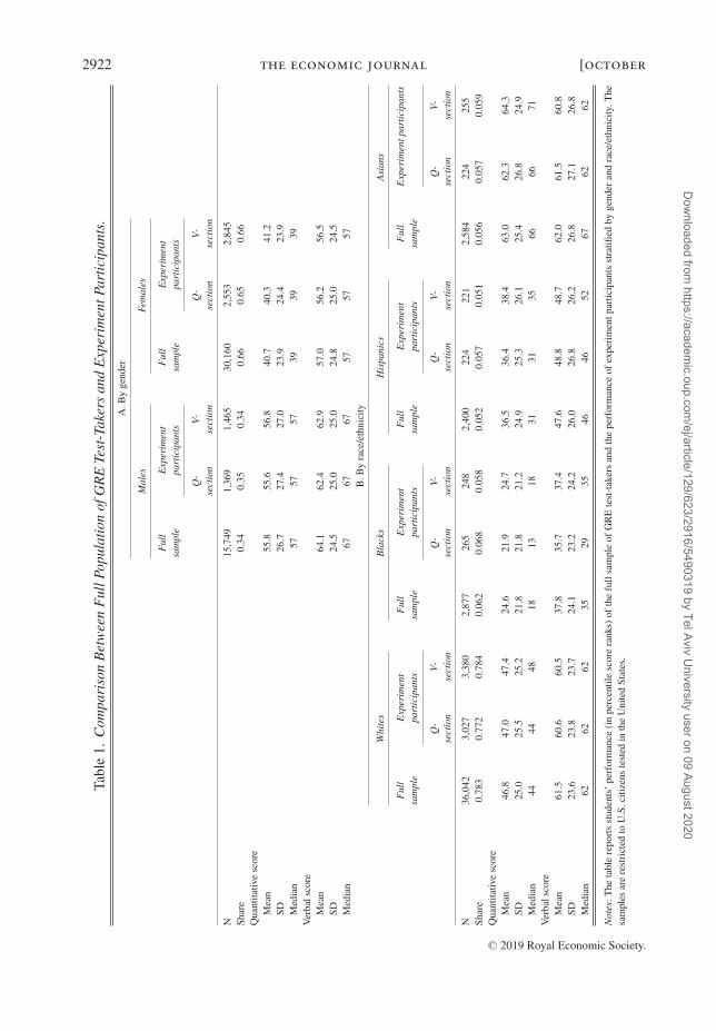
A unique feature of our research design that distinguishes our study from most of the experi-mental literature is that we are able to identify and characterise the experiment participants out ofthe full population of interest (i.e., GRE examinees in our case). Table 1 compares the character-istics of the full sample of U.S. GRE test-takers and the sample of experiment participants.10 Thetwo populations are virtually identical in terms of proportions of females, males and minorities.For example, women constitute 66% of the full population of U.S. domestic examinees, while theshare of women among those who agreed to participate in the Q- or the V-section was 65% and66% respectively. Likewise, whites make up about 78% of GRE U.S. domestic examinees andthey are similarly represented among experiment participants. The shares of blacks, Hispanicsand Asians range between 6% and 5.5% in both the full sample and the sample of experimentparticipants.11
Participants in the experiment also have similar GRE test scores to those in the full relevantsub-population from which they were drawn. For example, males are located, on average, at the56 percentile rank of the Q-score distribution, which is equal to the average performance of maleparticipants in the experiment. The median score (57 percentile rank) and standard deviation(27 points) are also identical for the full sample of GRE U.S. male test-takers, the sample ofexperiment participants randomised to the Q-section, and the sample of experiment participantsrandomised to the V-section. The test score distribution of female GRE test-takers is also identicalto that of female experiment participants. We observe also the same result when comparing test-score distributions within each race/ethnicity. Overall, the results presented in Table 1 show thatthere is no differential selection into the experiment according to gender, race/ethnicity or GREtest scores; nor do we find any evidence of differential selection within each gender or race/ethnicgroup.12
GRE test-takers are required to fill out a form upon registration to the exam. The form collectsinformation on basic background characteristics, college studies and intended graduate field ofstudies.13 Appendix Table A2 reports the descriptive statistics of these background characteristics
8 Since the experimental sections were randomised among the full sample of experiment participants, which includedall students (U.S. and international) tested in all centres around the world, the proportion of U.S. participants assigned toeach section is not exactly 50%.
9 One limitation of our study is that we were not able to randomise the order of the tests, so that all examinees receivedthe low stakes test after the high stakes test. As we discuss below, we believe that this constraint does not affect our mainresults or interpretation.
10 Owing to data restrictions, we cannot compare experiment participants to non-participants because we receivedthe data on experiment participants and the data on the full population of GRE examinees in two separate data sets thatlacked individual identifiers.
11 Reported proportions by race/ethnicity do not add up to one because the following additional groups are not reportedin the table: American Indian, Alaskan, and examinees with missing race/ethnicity.
12 While we do not find differences in observable characteristics, there could still be differences in unobservedcharacteristics. Nevertheless, for the purpose of our study, we should worry about differential selection into the experimentby unobservables across demographic groups. The fact that we did not find evidence for differential selection acrossgroups according to observables suggests that the presence of large differences in selection by unobservables acrossgroups is very unlikely.
13 We obtained the complete background information on experiment participants only, so we only analyse selectionin the experiment according to gender, race, ethnicity and GRE scores in the high stakes section.
C© 2019 Royal Economic Society.
Dow
nloaded from https://academ
ic.oup.com/ej/article/129/623/2916/5490319 by Tel Aviv U
niversity user on 09 August 2020
2922 the economic journal [october
Tabl
e1.
Com
pari
son
Bet
wee
nF
ullP
opul
atio
nof
GR
ETe
st-T
aker
san
dE
xper
imen
tPar
tici
pant
s.
A.B
yge
nder
Mal
esFe
mal
es
Ful
lsa
mpl
eE
xper
imen
tpa
rtic
ipan
tsF
ull
sam
ple
Exp
erim
ent
part
icip
ants
Q-
sect
ion
V-
sect
ion
Q-
sect
ion
V-
sect
ion
N15
,749
1,36
91,
465
30,1
602,
553
2,84
5Sh
are
0.34
0.35
0.34
0.66
0.65
0.66
Qua
ntita
tive
scor
eM
ean
55.8
55.6
56.8
40.7
40.3
41.2
SD26
.727
.427
.023
.924
.423
.9M
edia
n57
5757
3939
39V
erba
lsco
reM
ean
64.1
62.4
62.9
57.0
56.2
56.5
SD24
.525
.025
.024
.825
.024
.5M
edia
n67
6767
5757
57B
.By
race
/eth
nici
ty
Whi
tes
Bla
cks
His
pani
csA
sian
s
Ful
lsa
mpl
eE
xper
imen
tpa
rtic
ipan
tsF
ull
sam
ple
Exp
erim
ent
part
icip
ants
Ful
lsa
mpl
eE
xper
imen
tpa
rtic
ipan
tsF
ull
sam
ple
Exp
erim
entp
arti
cipa
nts
Q-
sect
ion
V-
sect
ion
Q-
sect
ion
V-
sect
ion
Q-
sect
ion
V-
sect
ion
Q-
sect
ion
V-
sect
ion
N36
,042
3,02
73,
380
2,87
726
524
82,
400
224
221
2,58
422
425
5Sh
are
0.78
30.
772
0.78
40.
062
0.06
80.
058
0.05
20.
057
0.05
10.
056
0.05
70.
059
Qua
ntita
tive
scor
eM
ean
46.8
47.0
47.4
24.6
21.9
24.7
36.5
36.4
38.4
63.0
62.3
64.3
SD25
.025
.525
.221
.821
.821
.224
.925
.326
.125
.426
.824
.9M
edia
n44
4448
1813
1831
3135
6666
71V
erba
lsco
reM
ean
61.5
60.6
60.5
37.8
35.7
37.4
47.6
48.8
48.7
62.0
61.5
60.8
SD23
.623
.823
.724
.123
.224
.226
.026
.826
.226
.827
.126
.8M
edia
n62
6262
3529
3546
4652
6762
62
Not
es:T
heta
ble
repo
rts
stud
ents
’pe
rfor
man
ce(i
npe
rcen
tile
scor
era
nks)
ofth
efu
llsa
mpl
eof
GR
Ete
st-t
aker
san
dth
epe
rfor
man
ceof
expe
rim
entp
artic
ipan
tsst
ratifi
edby
gend
eran
dra
ce/e
thni
city
.The
sam
ples
are
rest
rict
edto
U.S
.citi
zens
test
edin
the
Uni
ted
Stat
es.
C© 2019 Royal Economic Society.
Dow
nloaded from https://academ
ic.oup.com/ej/article/129/623/2916/5490319 by Tel Aviv U
niversity user on 09 August 2020
2019] performance in high vs. low stakes tests 2923
for the sample of experiment participants stratified by gender, race and ethnicity. Note that thecomparisons presented here are across the population of GRE test-takers, which is a selectedsample of college students, and therefore they do not represent group differences across thepopulation of college students but rather differences across college students who intend to pursuegraduate studies.
Averages reported in columns 2 and 3 of Table A2 show that males and females come fromsimilar family backgrounds, as measured by both mother’s and father’s educational levels and bythe proportion of native English speakers. Females and males also have similar distributions ofundergraduate GPA (UGPA). Nevertheless, males are more likely to come from undergraduatemajors in math, computer science, physics or engineering, and they are also more likely to intendto pursue graduate studies in these fields (26% for males versus 5% for females).
Columns 3 through 6 in Table A2 report descriptive statistics of the analysis sample stratifiedby race/ethnicity. Maternal education is similar among whites and Asians, but Asians are morelikely to have a father with at least some graduate studies or a professional degree relative towhites (45% versus 35%). Hispanics and blacks come from less educated families. Asians are lesslikely to be native English speakers (86%) relative to whites (93%), blacks (95%) and Hispanics(90%). In terms of undergraduate achievement, we observe that whites and Asians have similarUGPA distributions, but Hispanics and blacks have, on average, lower UGPAs. Asians are morelikely to do math, science and engineering either as an undergraduate major or as an intendedfield of graduate studies (30%) relative to whites (11%), blacks (8%) or Hispanics (12%).
2. Empirical Framework
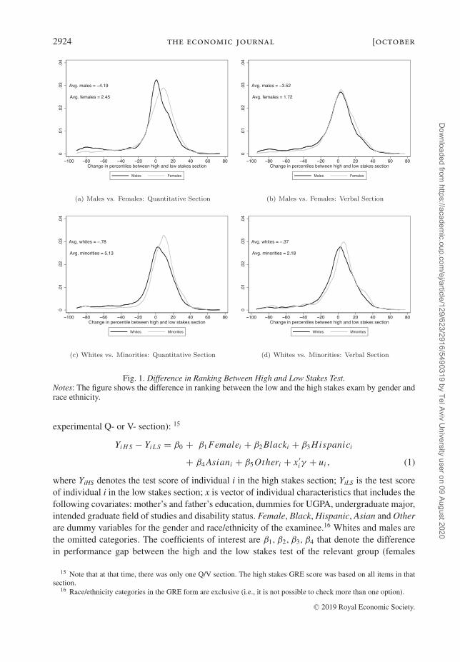
Our main objective is to examine how the performance of different demographic groups changesas a function of the stakes of the test (high stakes: real GRE exam; low stakes: experimentalsection). We summarise our main finding in Figure 1, using an ordinal metric, which is free ofthe specific scale of test scores. We ranked individuals according to their performance in eachtest and plot the rank change distribution (in percentile points) between the high and low stakestest by gender and race for each test. Panels (a) and (b) show that men’s ranking declines by 4percentile points in the low stakes test relative to the high stakes test, while women’s rankingimproves by 2 percentile points. Panels (c) and (d) show that the ranking of whites declines whilethe ranking of minorities improves when switching from the high to the low stakes test in both theQ- and the V-section. Focusing on the Q-section, which is less likely to be affected by languageproblems of minorities, we see that whites’ ranking declined by almost 1 percentile point whilethat of minorities improved by about 5 percentile points.14 The rank changes between men andwomen and between whites and minorities are statistically different (p-values of Mann–Whitneytests < 0.0001).
We now turn to measure individuals’ change in performance using a simple regression modelto control for additional characteristics of individuals and quantify the average change in per-formance between the high and low stakes test for each group. We estimate the following firstdifference equation for each of the experimental samples (i.e., individuals randomised to the
14 Minorities include Asians, Hispanics and blacks. We excluded students who defined themselves as American Indianor Alaskan Native (43) or other race (271).
C© 2019 Royal Economic Society.
Dow
nloaded from https://academ
ic.oup.com/ej/article/129/623/2916/5490319 by Tel Aviv U
niversity user on 09 August 2020
2924 the economic journal [october
Fig. 1. Difference in Ranking Between High and Low Stakes Test.Notes: The figure shows the difference in ranking between the low and the high stakes exam by gender andrace ethnicity.
experimental Q- or V- section): 15
YiHS − YiLS = β0 + β1Femalei + β2Blacki + β3Hispanici
+ β4Asiani + β5Otheri + x ′iγ + ui, (1)
where YiHS denotes the test score of individual i in the high stakes section; YiLS is the test scoreof individual i in the low stakes section; x is vector of individual characteristics that includes thefollowing covariates: mother’s and father’s education, dummies for UGPA, undergraduate major,intended graduate field of studies and disability status. Female, Black, Hispanic, Asian and Otherare dummy variables for the gender and race/ethnicity of the examinee.16 Whites and males arethe omitted categories. The coefficients of interest are β1, β2, β3, β4 that denote the differencein performance gap between the high and the low stakes test of the relevant group (females
15 Note that at that time, there was only one Q/V section. The high stakes GRE score was based on all items in thatsection.
16 Race/ethnicity categories in the GRE form are exclusive (i.e., it is not possible to check more than one option).
C© 2019 Royal Economic Society.
Dow
nloaded from https://academ
ic.oup.com/ej/article/129/623/2916/5490319 by Tel Aviv U
niversity user on 09 August 2020
2019] performance in high vs. low stakes tests 2925
Table 2. Performance in GRE Test by Gender, Race and Ethnicity.Males (M) Females (F) M-F Whites (W) Blacks (B) Hispanics (H) Asians (A) W-B W-H W-A
(1) (2) (3) (4) (5) (6) (7) (8) (9) (10)
(a) High stakes scoreQuantitative section 55.58 40.28 15.30 46.99 21.85 36.39 62.30 25.13 10.59 − 15.32
(27.43) (24.38) (0.85) (25.46) (21.80) (25.33) (26.76) (1.62) (1.75) (1.75)Number of observations 1368 2553 3026 265 224 224Verbal section 62.90 56.45 6.45 60.55 37.37 48.73 60.84 23.18 11.82 − 0.30
(24.96) (24.54) (0.79) (23.69) (24.23) (26.20) (26.85) (1.58) (1.67) (1.56)Number of observations 1465 2845 3380 248 221 255(b) Low stakes scoreQuantitative section 43.93 33.16 10.77 37.55 18.90 32.58 55.20 18.65 4.97 − 17.64
(31.34) (25.48) (0.93) (27.78) (19.72) (26.39) (30.38) (1.75) (1.90) (1.90)Number of observations 1368 2553 3026 265 224 224Verbal section 52.48 50.34 2.14 52.79 35.08 42.22 51.78 17.71 10.57 1.01
(30.53) (27.65) (0.92) (28.17) (24.08) (27.87) (31.42) (1.85) (1.95) (1.83)Number of observations 1465 2845 3380 248 221 255
Notes: The table reports students’ test scores in the high stakes and low stakes sections of the GRE and the gaps between males and females, and whites andminorities. Test scores are reported in percentile ranks. Standard deviations are reported in parenthesis.
or blacks/Hispanics/Asians) relative to the omitted category (males or whites). To simplify theexposition, we reverse the sign of the coefficients and report in all tables differences betweenmales and females and differences between whites and blacks/Hispanics/Asians.
Note that by using a first difference specification we are differencing out an individual’sfixed effect that accounts for all factors that affect examinee’s performance in both the lowstakes and the high stakes test. By including a vector of covariates, we allow for an individual’scharacteristics to affect the change in performance between the high and low stakes situation.17
GRE scores in the quantitative and verbal sections range between 200 and 800, in 10-pointincrements. To ease the interpretation of the results, we transformed these raw scores intopercentile ranks using the GRE official percentile rank tables.18 All results presented below arebased on GRE percentile ranks. As we show below, we obtain similar results when using rawscores, log of raw scores or z-scores.
3. Results
3.1. Differences in Performance by Gender, Race and Ethnicity
Panel (a) of Table 2 exhibits examinees’ performance in the high stakes test for males, females,whites, blacks, Hispanics, and Asians and the gaps between groups.19 Similar to other compar-
17 An alternative approach is to estimate a conditional model that regresses the score in the low stakes test on thescore in the high stakes test. The score-change model described in equation (1) and the conditional regression modelboth attempt to adjust for baseline outcomes but they answer different questions. The score-change model examines howgroups, on average, differ in score changes between the high and the low stakes test. The conditional regression model askswhether the score change of an individual who belongs to one group differs from the score change of an individual whobelongs to another group under the assumption that the two had come from a population with the same baseline level. Thetwo approaches are expected to provide equivalent answers when the groups have similar baseline outcomes. However,as discussed by Cribbie and Jamieson (2000), when baseline means differ between groups, conditional regression suffersfrom directional bias. Namely, conditional regression augments differences when groups start at different levels and thenremain parallel or diverge (see Lord’s Paradox—Lord, 1967) and attenuates differences when groups start at differentlevels and then converge. Because the demographic groups we examine have different baseline GRE performance, wechoose to estimate models of score change.
18 For more information regarding on the interpretation of GRE scores, exam administration and validity, see Educa-tional Testing Service (2007).
19 The percentile scores of males and females do not add to 100 since they are constructed using the official GREtables, which include international examinees and are based on several years of data.
C© 2019 Royal Economic Society.
Dow
nloaded from https://academ
ic.oup.com/ej/article/129/623/2916/5490319 by Tel Aviv U
niversity user on 09 August 2020
2926 the economic journal [october
isons of GRE scores by gender, males outperform females in both the quantitative and verbalsections among the participants in our experiment. On average, males are placed about 15.3percentile points higher in the test-score distribution of the Q-section relative to females. Thegender gap in the V-section is smaller but still sizable, with males scoring about 6.5 percentilepoints higher than females. Asians have the highest achievements among all ethnic/racial groupsin the Q-section. Their test scores are about 15 percentile points above those of whites. Hispanicslag behind whites by an average of 10.6 percentile points. Q-scores of blacks are lower, and theyare placed, on average, about 25 percentile points below whites in the test-score distribution.In the verbal section, whites outperform Asians, although the difference between groups is notstatistically significant. The gap between whites and blacks is a bit smaller (23 percentile points),while the gap between whites and Hispanics is about 12 percentile points. With the exception ofwhites versus Asians in the verbal section, all gaps between groups in the high stakes section arestatistically significant.
Panel (b) of Table 2 reports students’ performance in the experimental section and gaps bygender and race/ethnicity. On average, performance in the low stakes test is lower than in thehigh stakes test for all groups. Notably, gaps between males and females or whites and blacksor Hispanics are narrower in the experimental section (even though they are still statisticallysignificant). For example, the score gap between males and females shrinks from 15 to 11percentile points in the Q-section and from 7 to 2 percentile points in the V-section. The scoregap between whites and blacks shrinks from 25 to 19 percentile points in the Q-section andfrom 23 to 18 in the V-section, and the gap between whites and Hispanics shrinks from 11 to 5percentile points in the Q-section and from 12 to 11 percentile points in the V-section. The gapbetween Asians and whites in the Q-section widens between the high and the low stakes test(from 15 to 18 percentile points) because Asians outperform whites in this exam.
Table 3 reports the change in performance between the high and the low stakes section for eachdemographic group (first row of each panel) and the difference (second and third rows) in thedrop in performance between males and females or between whites and blacks/Hispanics/Asians.Males’ performance drops by 11.6 percentile points from the high to the low stakes Q-sections,while females’ performance drops by only 7.1 points. The gap in the drop in performancebetween males and females is significant and stands at 4.5 percentile points (SE = 0.784). Thatis, a switch from the high to the low stakes situation narrows the gender gap in the quantitativetest by about 4.5 percentile points (although it is still significant), which is equivalent to a 30%drop in the gender gap of the high stakes test. The differential change in performance remainsalmost unchanged after controlling for individual’s background characteristics and academicachievement. This finding is important as it suggests that our results are unlikely to be driven bydifferences in family background and academic achievement.
We also find a similar gender gap in the V-section. Males’ scores drop by 10.4 percentilepoints, on average, while females’ scores drop by a smaller magnitude of 6.1 percentile points.That is, males’ scores drop by 4.3 percentile points (SE = 0.783) more relative to females. Notethat the proportional drop in males’ performance is also larger than females’. Namely, males’scores drop by 21% while females’ scores drop by 18% in the Q-section. Similarly, we find thatmales’ scores in the V-section drop by 17% while females’ scores drop by 11%.
The stratification by race/ethnicity shows that whites exhibit the largest drop in performancebetween the high and the low stakes Q-section. Whites’ performance drops by 9.4 percentilepoints, while Asians’ performance drops by 7 percentile points, blacks’ performance drops by3 percentile points and Hispanics’ performance drops by 3.8 percentile points. Differences in
C© 2019 Royal Economic Society.
Dow
nloaded from https://academ
ic.oup.com/ej/article/129/623/2916/5490319 by Tel Aviv U
niversity user on 09 August 2020
2019] performance in high vs. low stakes tests 2927
Table 3. Difference in Performance Between High and Low Stakes Test by Gender, Race andEthnicity.
Males Females Whites Blacks Hispanics Asians(1) (2) (3) (4) (5) (6)
(a) Quantitative sectionHigh stakes − low stakes 11.644 7.115 9.431 2.951 3.808 7.107
(0.683) (0.385) (0.399) (0.863) (1.346) (1.561)Raw difference between males andfemales or whites and minority group
4.529 6.480 5.623 2.323(0.784) (0.949) (1.402) (1.609)
Controlled difference 3.905 4.276 5.205 3.145(0.820) (1.050) (1.402) (1.701)
(b) Verbal sectionHigh stakes – low stakes 10.421 6.108 7.755 2.282 6.511 9.067
(0.673) (0.400) (0.390) (1.316) (1.457) (1.625)Raw difference between males andfemales or whites and minority group
4.313 5.473 1.244 − 1.312(0.783) (1.371) (1.506) (1.669)
Controlled difference 3.577 3.150 0.629 − 0.555(0.821) (1.472) (1.533) (1.706)
Notes: The first row of each panel reports differences in individual’s performance between the high and the low stakes section of the GREby gender, race and ethnicity. The second row of each panel reports the differences in the drop in performance between males and femalesor whites and blacks/Hispanics/Asians. The third row of each panel reports differences between groups controlling for the followingindividual covariates: mother’s and father’s education, indicators for gender or race/ethnicity, UGPA, undergraduate major, intendedgraduate field of studies and disability status. Test scores are reported in percentile ranks. Robust standard deviations and standard errorsof the differences are reported in parentheses.
the performance drop between whites and each of the minority groups are all significant. Thecontrolled difference between whites and blacks, after accounting for individual’s characteristics,is of 4.3 percentile points (SE = 1.05). The equivalent difference between whites and Hispanicsis 5.21 (SE = 1.40) and the difference between whites and Asians is 3.2 (SE = 1.70). In the verbalsection, the performance drop from the high to the low stakes section is larger for whites thanfor blacks (7.8 percentile points versus 2.3 percentile points). But Hispanics and Asians exhibita similar drop in performance to that of whites. We suspect that the different pattern obtained forAsians and Hispanics in the V-section could be related to language dominance.
Overall, the evidence presented in Table 3 shows that males and whites exhibit the largestdrop in performance between the high and the low stakes tests compared with females andminorities. Our results are robust to non-linear transformations and alternative definitions of thedependent variable, as reported in Appendix Table A3. In the first row of panels (a) and (b), wereport differences in performance in the quantitative and verbal sections using raw scores (scaledbetween 200 and 800). In the second row of each panel, we show differences in performanceusing the natural logarithm of raw scores. In the third row, we report results based on z-scores.20
All alternative metrics yield results that are equivalent to our main findings: males’ drop inperformance between the high and low stakes section is 5% or 0.17 SD larger than the drop offemales; whites’ drop in performance in the Q-section is 8% or 0.23 SD larger than the drop ofblacks; 7% or 0.23 SD larger than the drop of Hispanics and 7% or 0.19 SD larger than the dropof Asians. These additional results show that our findings are not driven by a specific scale usedto measure achievement. Furthermore, as we show in Figure 1, we obtain the same results whenwe rely only on the ordinal information embedded in scores.
The fourth row of each panel in Table A3 replicates our main results using the samples ofexaminees randomised into experimental sections with extended time limits (67.5 minutes for the
20 Z-scores are computed using the mean and standard deviation of the high stakes test.
C© 2019 Royal Economic Society.
Dow
nloaded from https://academ
ic.oup.com/ej/article/129/623/2916/5490319 by Tel Aviv U
niversity user on 09 August 2020
2928 the economic journal [october
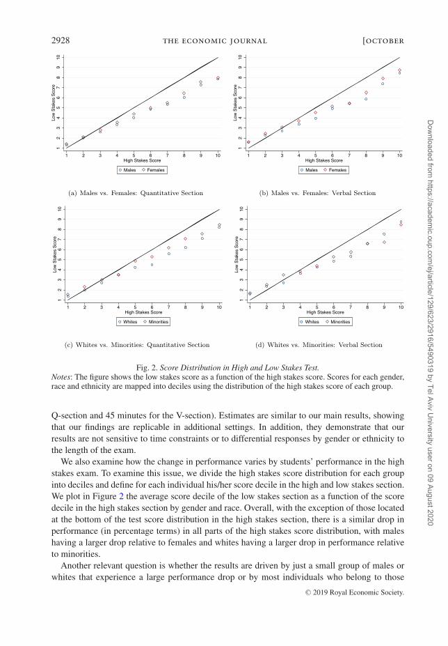
Fig. 2. Score Distribution in High and Low Stakes Test.Notes: The figure shows the low stakes score as a function of the high stakes score. Scores for each gender,race and ethnicity are mapped into deciles using the distribution of the high stakes score of each group.
Q-section and 45 minutes for the V-section). Estimates are similar to our main results, showingthat our findings are replicable in additional settings. In addition, they demonstrate that ourresults are not sensitive to time constraints or to differential responses by gender or ethnicity tothe length of the exam.
We also examine how the change in performance varies by students’ performance in the highstakes exam. To examine this issue, we divide the high stakes score distribution for each groupinto deciles and define for each individual his/her score decile in the high and low stakes section.We plot in Figure 2 the average score decile of the low stakes section as a function of the scoredecile in the high stakes section by gender and race. Overall, with the exception of those locatedat the bottom of the test score distribution in the high stakes section, there is a similar drop inperformance (in percentage terms) in all parts of the high stakes score distribution, with maleshaving a larger drop relative to females and whites having a larger drop in performance relativeto minorities.
Another relevant question is whether the results are driven by just a small group of males orwhites that experience a large performance drop or by most individuals who belong to those
C© 2019 Royal Economic Society.
Dow
nloaded from https://academ
ic.oup.com/ej/article/129/623/2916/5490319 by Tel Aviv U
niversity user on 09 August 2020
2019] performance in high vs. low stakes tests 2929
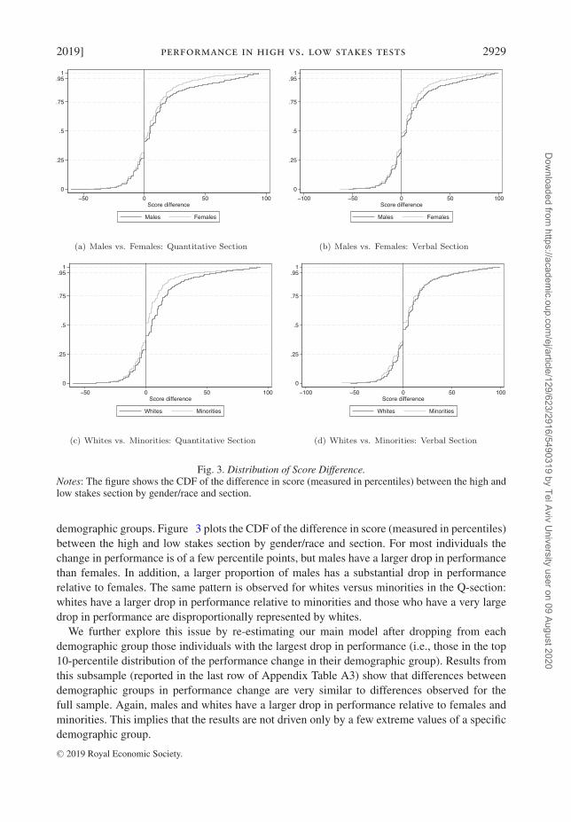
Fig. 3. Distribution of Score Difference.Notes: The figure shows the CDF of the difference in score (measured in percentiles) between the high andlow stakes section by gender/race and section.
demographic groups. Figure 3 plots the CDF of the difference in score (measured in percentiles)between the high and low stakes section by gender/race and section. For most individuals thechange in performance is of a few percentile points, but males have a larger drop in performancethan females. In addition, a larger proportion of males has a substantial drop in performancerelative to females. The same pattern is observed for whites versus minorities in the Q-section:whites have a larger drop in performance relative to minorities and those who have a very largedrop in performance are disproportionally represented by whites.
We further explore this issue by re-estimating our main model after dropping from eachdemographic group those individuals with the largest drop in performance (i.e., those in the top10-percentile distribution of the performance change in their demographic group). Results fromthis subsample (reported in the last row of Appendix Table A3) show that differences betweendemographic groups in performance change are very similar to differences observed for thefull sample. Again, males and whites have a larger drop in performance relative to females andminorities. This implies that the results are not driven only by a few extreme values of a specificdemographic group.
C© 2019 Royal Economic Society.
Dow
nloaded from https://academ
ic.oup.com/ej/article/129/623/2916/5490319 by Tel Aviv U
niversity user on 09 August 2020
2930 the economic journal [october
Table 4. Performance in High versus Low Stakes Tests by Gender andRace/Ethnicity—Quantitative Section.
High stakes Low stakes High − low stakesControlleddifference
Males Females Males Females Males Females (Males − Females)(1) (2) (3) (4) (5) (6) (7)
Whites 56.701 41.800 43.914 34.161 12.787 7.639 4.904(26.403) (23.342) (25.179) (31.132) (0.793) (0.437) (0.945)
Blacks 28.769 19.605 24.215 17.175 4.554 2.430 0.186(27.739) (19.039) (16.851) (26.150) (2.146) (0.906) (2.531)
Controlled difference 5.485 3.568(Whites − blacks) (2.405) (1.153)Hispanics 44.022 31.363 38.405 28.748 5.618 2.615 0.181
(27.048) (22.875) (23.230) (29.775) (2.422) (1.561) (3.502)Controlled difference 7.464 4.071(Whites − Hispanics) (2.608) (1.663)Asians 72.167 56.386 66.071 48.671 6.095 7.714 − 1.307
(23.589) (26.875) (29.090) (29.509) (2.603) (1.955) (4.678)Controlled difference 9.266 − 0.399(Whites − Asians) (2.955) (2.055)
Notes: The table reports test scores in the Q-section of the GRE exam. Columns 1–2 report mean performance in the high stakes test foreach gender–race/ethnicity group. Columns 3–4 report mean performance in the low stakes test for each gender–race/ethnicity group.Performance change between the high and the low stakes tests are reported in columns 5 and 6. Controlled differences in performancechange between males and females stratified by race/ethnicity are reported in bold in column 7. Test scores are reported in percentileranks. Standard deviations and robust standard errors are reported in parentheses.
3.2. Within Race/Ethnicity and Gender Differences in Performance
We check for gender and race/ethnicity interactions by examining whether differences betweenmales and females appear across all racial/ethnic groups and whether differences between whitesand minorities show up for males and for females.21
Table 4 reports performance in the high and low stakes section for each gender and eth-nicity/race as well as differences in performance between males and females within eachrace/ethnicity and between whites and minorities for males and females separately. We focus onthe Q-section, as performance is less influenced by language constraints among Hispanics andAsians. The results show that white males have the largest differential performance between thehigh and the low stakes test compared to Black, Asian and Hispanic males. We obtain a similarresult for females with the exception of Asian females, who behave similarly to white females.
Comparisons between males and females within each racial/ethnic group reveal that malesexhibit a larger drop in performance than females among whites, blacks and Hispanics, althoughdifferences between genders are only statistically significant among whites. In contrast, weobserve no gender differences among Asians. In fact, the drop observed among females is evenlarger than the drop observed among males, although the difference is not statistically significant.
3.3. Heterogeneous Effects
Table 5 reports the gender gap in students’ performance in high and low stakes tests for differentsubsamples stratified by undergraduate GPA (UGPA), student’s major, intended field of graduatestudies and mother’s education. We focus on gender gap and not on gap by race/ethnicity, since
21 The conclusions described in this subsection rely on samples that are stratified by gender and race/ethnicity andthat are relatively small for blacks, Hispanics and Asians, so the results should be taken with caution.
C© 2019 Royal Economic Society.
Dow
nloaded from https://academ
ic.oup.com/ej/article/129/623/2916/5490319 by Tel Aviv U
niversity user on 09 August 2020
2019] performance in high vs. low stakes tests 2931
Tabl
e5.
Perf
orm
ance
inH
igh
and
Low
Stak
esTe
sts
byG
ende
ran
dE
xam
inee
Cha
ract
eris
tics
.
Num
ber
ofob
s.H
igh
stak
essc
ore
Low
stak
essc
ore
Hig
hst
akes
−lo
wst
akes
Mal
esFe
mal
esM
ales
Fem
ales
Diff
.M
ales
Fem
ales
Diff
.M
ales
Fem
ales
Raw
diff.
Con
trol
led
diff.
(1)
(2)
(3)
(4)
(5)
(6)
(7)
(8)
(9)
(10)
(11)
(12)
(a)
Qua
ntit
ativ
ese
ctio
nU
nder
grad
uate
GPA
Cor
C−
102
134
39.7
8421
.157
18.6
2830
.461
18.5
9011
.871
9.32
42.
567
6.75
67.
103
(24.
462)
(18.
445)
(2.7
93)
(17.
397)
(25.
557)
(2.8
00)
(1.9
47)
(0.8
51)
(2.1
24)
(2.3
20)
B−
144
266
43.0
2828
.267
14.7
6134
.458
24.0
3410
.425
8.56
94.
233
4.33
62.
295
(25.
528)
(19.
377)
(2.2
48)
(19.
386)
(26.
841)
(2.3
06)
(1.9
39)
(0.8
37)
(2.1
11)
(2.2
94)
B42
685
548
.962
36.0
6312
.899
38.4
1829
.958
8.46
010
.545
6.10
54.
439
3.49
2(2
5.94
2)(2
2.75
5)(1
.415
)(2
3.05
6)(2
8.66
0)(1
.486
)(1
.152
)(0
.613
)(1
.305
)(1
.375
)A
−39
371
763
.237
46.8
1516
.422
51.4
3837
.756
13.6
8211
.799
9.05
92.
740
3.10
9(2
4.90
6)(2
3.93
5)(1
.524
)(2
7.15
0)(3
1.76
5)(1
.812
)(1
.273
)(0
.823
)(1
.516
)(1
.641
)A
251
490
69.8
2150
.700
19.1
2153
.801
42.3
8211
.419
16.0
208.
318
7.70
27.
980
(25.
227)
(23.
462)
(1.8
69)
(27.
321)
(34.
295)
(2.3
18)
(1.9
08)
(0.9
59)
(2.1
35)
(2.5
29)
Und
ergr
adm
ajor
in36
213
278
.644
69.9
558.
689
65.8
7063
.295
2.57
512
.773
6.65
96.
114
4.24
4ph
ysic
s,m
ath,
com
p.or
eng.
(17.
321)
(23.
107)
(1.9
35)
(27.
074)
(31.
352)
(3.0
78)
(1.5
49)
(2.1
21)
(2.6
24)
(2.8
29)
Gra
din
tend
edst
udie
sin
340
122
77.6
7470
.574
7.10
065
.515
64.3
691.
146
12.1
596.
205
5.95
44.
457
phys
ics,
mat
h,co
mp.
oren
g.(1
8.19
1)(2
1.70
7)(2
.024
)(2
5.90
9)(3
1.26
5)(3
.161
)(1
.596
)(2
.167
)(2
.689
)(2
.875
)M
ater
nale
duca
tion
Hig
hsc
hool
orle
ss32
058
243
.903
32.9
7310
.931
35.5
8127
.038
8.54
38.
322
5.93
52.
387
2.09
1(2
6.37
4)(2
2.98
6)(1
.687
)(2
3.11
7)(2
7.25
5)(1
.716
)(1
.235
)(0
.672
)(1
.405
)(1
.497
)C
olle
geor
som
eco
llege
621
1228
58.0
9739
.965
18.1
3246
.018
33.8
0012
.218
12.0
796.
165
5.91
45.
732
(26.
830)
(23.
495)
(1.2
14)
(24.
850)
(32.
199)
(1.3
56)
(1.0
13)
(0.5
29)
(1.1
42)
(1.2
18)
Atl
east
som
egr
adua
test
udie
sor
prof
essi
onal
degr
ee35
761
963
.588
48.7
2414
.864
49.9
5239
.069
10.8
8313
.636
9.65
43.
982
2.82
9(2
5.92
1)(2
5.12
5)(1
.689
)(2
7.69
7)(3
2.10
6)(1
.953
)(1
.455
)(0
.929
)(1
.725
)(1
.879
)
C© 2019 Royal Economic Society.
Dow
nloaded from https://academ
ic.oup.com/ej/article/129/623/2916/5490319 by Tel Aviv U
niversity user on 09 August 2020
2932 the economic journal [october
Tabl
e5.
Con
tinu
edN
umbe
rof
obs.
Hig
hst
akes
scor
eL
owst
akes
scor
eH
igh
stak
es−
low
stak
es
Mal
esFe
mal
esM
ales
Fem
ales
Diff
.M
ales
Fem
ales
Diff
.M
ales
Fem
ales
Raw
diff.
Con
trol
led
diff.
(1)
(2)
(3)
(4)
(5)
(6)
(7)
(8)
(9)
(10)
(11)
(12)
(b)
Ver
bals
ecti
onU
nder
grad
uate
GPA
Cor
C−
106
161
48.6
8938
.441
10.2
4843
.208
35.4
357.
773
5.48
13.
006
2.47
51.
121
(23.
915)
(22.
205)
(2.8
64)
(24.
116)
(26.
541)
(3.1
40)
(2.0
36)
(1.5
13)
(2.5
36)
(3.6
41)
B−
167
275
53.6
9547
.949
5.74
646
.144
44.4
471.
696
7.55
13.
502
4.04
90.
677
(26.
025)
(23.
273)
(2.3
89)
(25.
274)
(27.
002)
(2.5
45)
(1.7
19)
(1.1
29)
(2.0
56)
(2.5
83)
B43
694
558
.690
51.9
356.
755
50.1
9746
.309
3.88
88.
493
5.62
62.
867
2.51
4(2
3.90
5)(2
3.51
2)(1
.368
)(2
5.74
0)(2
9.11
7)(1
.555
)(1
.165
)(0
.664
)(1
.340
)(1
.392
)A
−40
579
968
.225
62.0
166.
208
54.1
3855
.253
−1.
115
14.0
866.
763
7.32
37.
098
(22.
888)
(23.
097)
(1.4
05)
(27.
634)
(32.
032)
(1.7
80)
(1.3
91)
(0.7
93)
(1.6
00)
(1.7
38)
A29
256
074
.137
66.3
667.
771
61.7
0958
.664
3.04
512
.428
7.70
24.
726
3.38
8(2
0.91
4)(2
2.57
3)(1
.589
)(2
8.62
2)(3
1.12
5)(2
.130
)(1
.598
)(0
.933
)(1
.850
)(2
.064
)U
nder
grad
maj
orin
388
161
66.7
8165
.839
0.94
254
.036
62.0
12−
7.97
612
.745
3.82
68.
919
7.54
7ph
ysic
s,m
ath,
com
p.or
eng.
(24.
124)
(25.
365)
(2.2
96)
(25.
708)
(31.
769)
(2.8
24)
(1.4
24)
(1.3
01)
(1.9
29)
(2.0
63)
Gra
din
tend
edst
udie
sin
378
142
66.3
4166
.056
0.28
553
.643
60.5
35−
6.89
212
.698
5.52
17.
177
7.50
6ph
ysic
s,m
ath,
com
p.or
eng.
(23.
796)
(24.
881)
(2.3
72)
(27.
411)
(31.
356)
(2.9
86)
(1.4
45)
(1.3
40)
(1.9
70)
(2.1
35)
Mat
erna
ledu
cati
onH
igh
scho
olor
less
344
628
54.3
0249
.244
5.05
945
.959
45.0
510.
908
8.34
34.
193
4.15
04.
197
(26.
892)
(23.
959)
(1.6
79)
(25.
717)
(29.
148)
(1.8
10)
(1.3
05)
(0.7
45)
(1.5
02)
(1.6
11)
Col
lege
orso
me
colle
ge65
813
5464
.114
56.0
788.
036
53.1
5749
.908
3.24
910
.957
6.17
14.
787
4.75
0(2
3.67
1)(2
3.94
2)(1
.134
)(2
7.13
9)(3
0.42
0)(1
.343
)(1
.033
)(0
.591
)(1
.190
)(1
.281
)A
tlea
stso
me
grad
uate
stud
ies
orpr
ofes
sion
alde
gree
376
731
68.8
3063
.848
4.98
258
.495
56.7
911.
704
10.3
357.
057
3.27
83.
614
(22.
931)
(24.
094)
(1.5
04)
(28.
787)
(30.
521)
(1.8
65)
(1.3
18)
(0.8
27)
(1.5
56)
(1.7
02)
Not
es:
The
tabl
ere
port
sge
nder
diff
eren
ces
inpe
rfor
man
cein
the
low
and
the
high
stak
esse
ctio
nsof
the
GR
Ete
stfo
rdi
ffer
ent
subs
ampl
es.
Pane
l(a
)re
port
sre
sults
for
expe
rim
ent
part
icip
ants
inth
eQ
-sec
tion;
pane
l(b)
repo
rts
resu
ltsfo
rex
peri
men
tpar
ticip
ants
inth
eV
-sec
tion.
Con
trol
led
diff
eren
ces
inco
lum
n12
incl
ude
the
cova
riat
esde
taile
din
Tabl
e2.
Test
scor
esar
ere
port
edin
perc
entil
era
nks.
Rob
usts
tand
ard
devi
atio
nsan
dst
anda
rder
rors
ofth
edi
ffer
ence
sar
ere
port
edin
pare
nthe
ses.
Sam
ple
size
sar
ere
port
edin
colu
mns
1an
d2.
C© 2019 Royal Economic Society.
Dow
nloaded from https://academ
ic.oup.com/ej/article/129/623/2916/5490319 by Tel Aviv U
niversity user on 09 August 2020
2019] performance in high vs. low stakes tests 2933
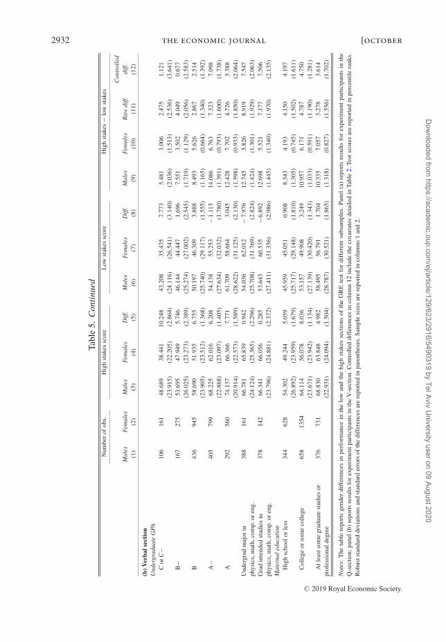
subgroups are too small for that stratification. Panel (a) reports results for the Q-section and panel(b) reports results for the V-section. Rows 1 through 5 in both panels present estimates for thesamples stratified by UGPA. As expected, students with higher UGPA have higher scores in boththe high and the low stakes sections of the quantitative and verbal exams. Males’ advantage in thehigh stakes test appears across all cells of the UGPA distribution, both in the quantitative and inthe verbal section. Again, we observe that the gender gap in performance is narrower in the lowstakes section in each of the cells stratified by UGPAs and is even insignificant when comparingperformance in the V-section between male and female students with an UGPA of A, A− or B−.
We see in columns 9 and 10 of the table that all students, regardless of their UGPA, exhibit asignificant drop in performance between the high and the low stakes sections (both the quantitativeand the verbal).22 Males’ performance drop is larger than females’ drop across all levels of UGPA(see columns 11 and 12), and is evident both in absolute and in percentage terms.
The next two rows of Table 5 (in both panels a and b) report the gender gap in performancefor the sample of students who majored in math, computer science, physics or engineering orwho intend to pursue graduate studies in one of these fields (to simplify the discussion, wewill call them math and science students). We focus on these students to target a population offemales that is expected to be highly selected.23 While females represent the majority among thefull population of GRE examinees (65%), they are a minority among math and science students(26%). It is therefore interesting to examine whether we find the same results in a subsamplewhere selection by gender goes in the opposite direction.
As seen in columns 3 and 4 of Table 5, achievement in the GRE Q-section is much higheramong math and science students relative to the full sample and even relative to those studentswhose UGPA is an ‘A’. Math and science students also attain higher scores in the V-sectionrelative to the full sample, but they score slightly lower compared with those students with an ‘A’UGPA. The gender gap in the high stakes Q-section among math and science students is smaller(8.7 percentile points) than the gender gap in the full sample (15.3 percentile points), although westill observe that males have higher achievement than females. The gender gap among those whointend to pursue graduate studies in these fields is even narrower (7.1 percentile points) althoughstill significant. In contrast, there is no gender gap achievement in the high stakes V-section inthe subsamples of math and science students.
Achievement of math and science students in the low stakes Q-section is lower than in the highstakes section, but these students still perform better relative to other students in the low stakessection. Consistent with our previous results, the gender gap in Q performance among math andscience students is narrower in the low stakes section relative to the high stakes section and iseven insignificant. The pattern for the V-section is similar, with math and science females evenoutperforming their male counterparts in the low stakes V-section.
Even in this subsample of math and science students, the drop in performance between thehigh and the low stakes test is larger for males (who reduce their performance by about 12–13percentile points in both subjects) compared with females (who reduce their performance by6–7 percentile points in the Q-section and by 4–5 percentile points in the V-section). The largerdrop in males’ performance is evident both in absolute terms and relative to the outcome means
22 We use UGPA to stratify the sample (instead of using the score in the high stakes section) because it provides ameasure of students’ performance that is taken independently and before the realisation of the dependent variable.
23 We focus here on a more limited number of fields than the traditional STEM (science, technology, engineering andmathematics) definition (e.g., we exclude biology) to select those fields that are predominately populated by males. Ourresults do not change when using the broader definition of STEM fields.
C© 2019 Royal Economic Society.
Dow
nloaded from https://academ
ic.oup.com/ej/article/129/623/2916/5490319 by Tel Aviv U
niversity user on 09 August 2020
2934 the economic journal [october
in the high stakes test. The gender differences in relative performance in these subsamples areabout 5 percentile points in the Q-section and 8 percentile points in the V-sections. Both gapsare statistically significant and do not change much after controlling for examinees’ observedcharacteristics. This finding is important because it shows that the larger drop in performanceamong males is found even in subsamples that exhibit no differences in performance in the highstakes test.
We also looked at gender gaps within groups stratified by mother’s education. We were curiousto check whether female examinees whose mothers attended graduate school would behave morelike males and exhibit a larger gap in performance between the high and low stakes situations.This turned out not to be the case. The gender gap in relative performance between high and lowstakes tests appears across all levels of maternal education in both the quantitative and the verbalsection.
4. Discussion
The evidence presented above shows that males and whites exhibit a larger difference in per-formance between high and low stakes tests compared with females and minorities. The largerdecline in performance found among males and whites could be due to at least distinct tworeasons: (i) males and whites do not exert as much effort in low stakes situations compared withfemales and minorities, respectively; (ii) females and minorities find it relatively more difficultto deal with high stakes and stressful situations.24 We examine below the plausibility of thesealternative explanations and discuss some other interpretations. We acknowledge that our datado not allow us to rigorously test the relative contribution of each explanation. Nevertheless, webelieve that the evidence presented below provides interesting directions for further research.
4.1. Do Males and Whites Exert Less Effort in Low Stakes Situations?
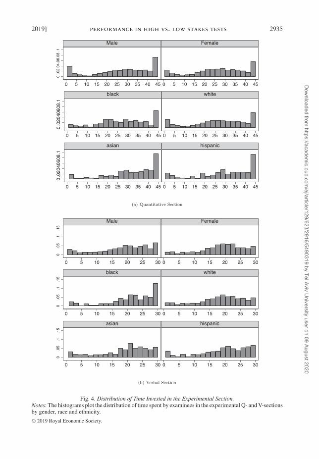
To examine the likelihood of the first explanation, we would ideally like to measure the effortinvested in the test. More effort could be exerted by trying harder to solve each question (i.e.,investment of more mental energy) or by investment of more time. Figure 4 plots the distributionof time spent by examinees in the experimental Q- and V-sections by gender, race and ethnicity.25
The figure shows that there is a significant variation in time invested in the experimental section.Some examinees spent very little time and some exhausted the time limit (45 minutes for theQ-section and 30 minutes for the V-section).
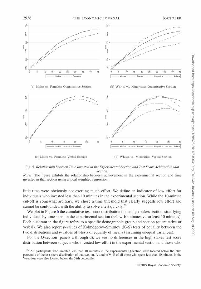
Figure 5 exhibits the relationship between achievement in the experimental section and thetime invested in that section for males, females, whites, blacks, Hispanics and Asians. The figureshows that achievement increases with time invested in the quantitative section for all gender,racial and ethnic groups. The relationship between time invested and performance in the verbalsection is also positive at the lower values of the distribution, but switches sign after about 20minutes. Overall, it is clear from the figures that it is impossible to receive a high score withoutinvesting some minimal amount of time. We therefore conclude that subjects who invested very
24 Alternatively, males and whites are arguably better able to boost their performance when stakes are high or the taskis challenging. This explanation is harder to assess as it is impossible to establish an ability baseline that is independentof performance in a given test of a given stake. It is challenging to even conceive of a thought experiment that couldpossibly answer this question because performance always depends on the perceived importance of the test.
25 Unfortunately, there is no information on time spent in the real GRE test. However, students usually exhaust thetime limit.
C© 2019 Royal Economic Society.
Dow
nloaded from https://academ
ic.oup.com/ej/article/129/623/2916/5490319 by Tel Aviv U
niversity user on 09 August 2020
2019] performance in high vs. low stakes tests 2935
Fig. 4. Distribution of Time Invested in the Experimental Section.Notes: The histograms plot the distribution of time spent by examinees in the experimental Q- and V-sectionsby gender, race and ethnicity.
C© 2019 Royal Economic Society.
Dow
nloaded from https://academ
ic.oup.com/ej/article/129/623/2916/5490319 by Tel Aviv U
niversity user on 09 August 2020
2936 the economic journal [october
Fig. 5. Relationship between Time Invested in the Experimental Section and Test Score Achieved in thatSection.
Notes: The figure exhibits the relationship between achievement in the experimental section and timeinvested in that section using a local weighted regression.
little time were obviously not exerting much effort. We define an indicator of low effort forindividuals who invested less than 10 minutes in the experimental section. While the 10-minutecut-off is somewhat arbitrary, we chose a time threshold that clearly suggests low effort andcannot be confounded with the ability to solve a test quickly.26
We plot in Figure 6 the cumulative test score distribution in the high stakes section, stratifyingindividuals by time spent in the experimental section (below 10 minutes vs. at least 10 minutes).Each quadrant in the figure refers to a specific demographic group and section (quantitative orverbal). We also report p-values of Kolmogorov–Smirnov (K–S) tests of equality between thetwo distributions and p-values of t-tests of equality of means (assuming unequal variances).
For the Q-section (panels a through d), we see no differences in the high stakes test scoredistribution between subjects who invested low effort in the experimental section and those who
26 All participants who invested less than 10 minutes in the experimental Q-section were located below the 58thpercentile of the test-score distribution of that section. A total of 94% of all those who spent less than 10 minutes in theV-section were also located below the 58th percentile.
C© 2019 Royal Economic Society.
Dow
nloaded from https://academ
ic.oup.com/ej/article/129/623/2916/5490319 by Tel Aviv U
niversity user on 09 August 2020
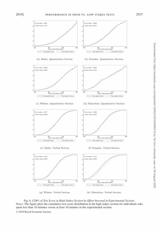
2019] performance in high vs. low stakes tests 2937
Fig. 6. CDFs of Test Score in High Stakes Section by Effort Invested in Experimental Section.Notes: The figure plots the cumulative test score distribution in the high stakes section for individuals whospent less than 10 minutes versus at least 10 minutes in the experimental section.
C© 2019 Royal Economic Society.
Dow
nloaded from https://academ
ic.oup.com/ej/article/129/623/2916/5490319 by Tel Aviv U
niversity user on 09 August 2020
2938 the economic journal [october
invested some reasonable amount of time. Indeed, we cannot reject the hypothesis of equalityof distributions or equality of means for each demographic group. This finding shows thatachievement in the high stakes section is unrelated to effort levels invested in the low stakessection, and implies that baseline differences in achievement in the high stakes section betweendemographic groups are unlikely to explain group differences in effort levels. Given that thechances of improving one’s score are probably lower for individuals who obtained higher scoresin the high stakes section, the result reported in Figure 6 suggests that individuals were notthinking about the chances of winning the prize when deciding about effort levels in the lowstakes section.
For the verbal section (panels e through h), we see no differences in test score distributions ormeans between those who invested low effort and others among males. We see some differencesin the test score distribution for females (p-value of K-S test = 0.04). Nevertheless, differencesin the distribution derive from differences in the dispersion around the mean, with a largervariance among those investing low effort. Indeed, we cannot reject the hypothesis of equalityof means between the two groups (p-value = 0.931). For minorities, we find lower effort levelsamong those with lower scores in the high stakes section (although the difference in distributionsis not statistically significant). These differences are the opposite of what we would expect ifexperiment participants were considering the monetary incentive when deciding about effortlevels in the low stakes test. Nevertheless, as discussed above, language difficulties might haveaffected performance of minorities in the verbal section, so we prefer not to put too much weightin the comparison of performance between whites and minorities in this section.
Taken together, the evidence presented in Figure 6 suggests that effort exerted by individualsin the experimental section is not related to performance in the ‘real’ GRE test across alldemographic groups in the Q-section, and among males, females and whites in the V-section.
Table 6 reports the share of examinees who invested less than 10 minutes in the experimental Q-and V-sections, stratified by gender, race/ethnicity, academic achievement and parental education.We also report p-values that test for equality of proportions between groups. The results showthat males appear to exert less effort in the experimental section compared with females: 17% ofthe males who participated in the Q-experiment spent less than 10 minutes in the experimentalsection, while the equivalent percentage among females is 13%. Gender differences are similarfor the V-section. It is important to recall that, as shown in Table 1, the share of males andfemales among experiment participants was equal to their share in the full population of GREtest-takers. This suggests that gender differences in effort among experiment participants cannotbe attributed to a differential selection into the experiment. Statistics by race/ethnicity show thatwhites are more likely to invest low effort relative to blacks and Asians. Whites also appear toinvest less effort than Hispanics, although differences in this case are smaller and not statisticallysignificant.
The stratification of the sample by background characteristics and achievement shows thatstudents with more educated parents are more likely to invest less in the exam. In contrast,we find no clear relationship between the likelihood of low effort and students’ achievement,neither when defined by students’ scores in the high stakes section nor when defined by students’UGPAs. This last finding is important as it shows that the decision to exert low effort in the lowstakes section is unrelated to students’ academic performance, suggesting that other factors arelikely to play a more important role in determining performance in low stakes situations. Thelack of a relationship between students’ academic performance and effort invested in the low
C© 2019 Royal Economic Society.
Dow
nloaded from https://academ
ic.oup.com/ej/article/129/623/2916/5490319 by Tel Aviv U
niversity user on 09 August 2020
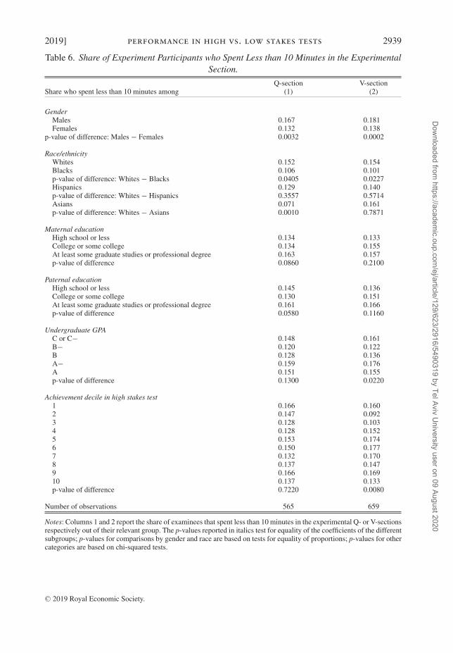
2019] performance in high vs. low stakes tests 2939
Table 6. Share of Experiment Participants who Spent Less than 10 Minutes in the ExperimentalSection.
Q-section V-sectionShare who spent less than 10 minutes among (1) (2)
GenderMales 0.167 0.181Females 0.132 0.138
p-value of difference: Males − Females 0.0032 0.0002
Race/ethnicityWhites 0.152 0.154Blacks 0.106 0.101p-value of difference: Whites − Blacks 0.0405 0.0227Hispanics 0.129 0.140p-value of difference: Whites − Hispanics 0.3557 0.5714Asians 0.071 0.161p-value of difference: Whites − Asians 0.0010 0.7871
Maternal educationHigh school or less 0.134 0.133College or some college 0.134 0.155At least some graduate studies or professional degree 0.163 0.157p-value of difference 0.0860 0.2100
Paternal educationHigh school or less 0.145 0.136College or some college 0.130 0.151At least some graduate studies or professional degree 0.161 0.166p-value of difference 0.0580 0.1160
Undergraduate GPAC or C− 0.148 0.161B− 0.120 0.122B 0.128 0.136A− 0.159 0.176A 0.151 0.155p-value of difference 0.1300 0.0220
Achievement decile in high stakes test1 0.166 0.1602 0.147 0.0923 0.128 0.1034 0.128 0.1525 0.153 0.1746 0.150 0.1777 0.132 0.1708 0.137 0.1479 0.166 0.16910 0.137 0.133p-value of difference 0.7220 0.0080
Number of observations 565 659
Notes: Columns 1 and 2 report the share of examinees that spent less than 10 minutes in the experimental Q- or V-sectionsrespectively out of their relevant group. The p-values reported in italics test for equality of the coefficients of the differentsubgroups; p-values for comparisons by gender and race are based on tests for equality of proportions; p-values for othercategories are based on chi-squared tests.
C© 2019 Royal Economic Society.
Dow
nloaded from https://academ
ic.oup.com/ej/article/129/623/2916/5490319 by Tel Aviv U
niversity user on 09 August 2020
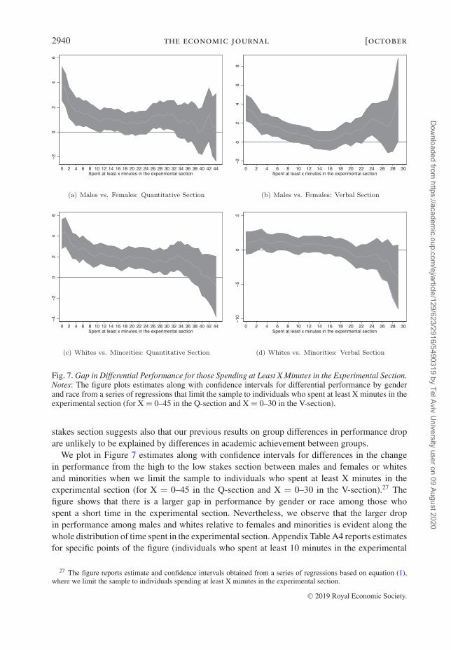
2940 the economic journal [october
Fig. 7. Gap in Differential Performance for those Spending at Least X Minutes in the Experimental Section.Notes: The figure plots estimates along with confidence intervals for differential performance by genderand race from a series of regressions that limit the sample to individuals who spent at least X minutes in theexperimental section (for X = 0–45 in the Q-section and X = 0–30 in the V-section).
stakes section suggests also that our previous results on group differences in performance dropare unlikely to be explained by differences in academic achievement between groups.
We plot in Figure 7 estimates along with confidence intervals for differences in the changein performance from the high to the low stakes section between males and females or whitesand minorities when we limit the sample to individuals who spent at least X minutes in theexperimental section (for X = 0–45 in the Q-section and X = 0–30 in the V-section).27 Thefigure shows that there is a larger gap in performance by gender or race among those whospent a short time in the experimental section. Nevertheless, we observe that the larger dropin performance among males and whites relative to females and minorities is evident along thewhole distribution of time spent in the experimental section. Appendix Table A4 reports estimatesfor specific points of the figure (individuals who spent at least 10 minutes in the experimental
27 The figure reports estimate and confidence intervals obtained from a series of regressions based on equation (1),where we limit the sample to individuals spending at least X minutes in the experimental section.
C© 2019 Royal Economic Society.
Dow
nloaded from https://academ
ic.oup.com/ej/article/129/623/2916/5490319 by Tel Aviv U
niversity user on 09 August 2020
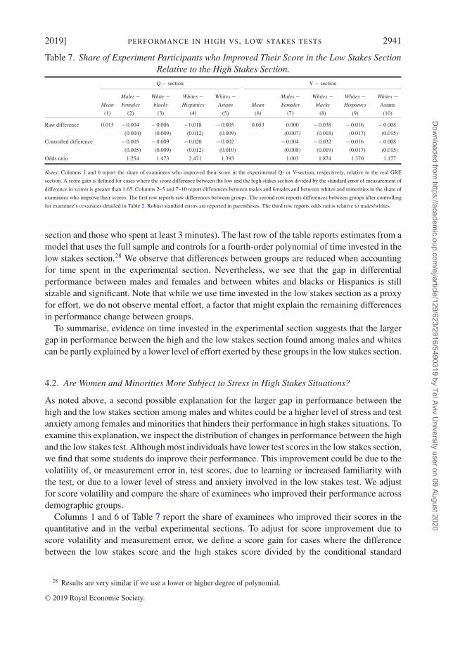
2019] performance in high vs. low stakes tests 2941
Table 7. Share of Experiment Participants who Improved Their Score in the Low Stakes SectionRelative to the High Stakes Section.
Q − section V − section
Mean
Males −Females
White −blacks
Whites −Hispanics
Whites −Asians Mean
Males −Females
Whites −blacks
Whites −Hispanics
Whites −Asians
(1) (2) (3) (4) (5) (6) (7) (8) (9) (10)
Raw difference 0.015 − 0.004 − 0.006 − 0.018 − 0.005 0.053 0.000 − 0.038 − 0.016 − 0.008
(0.004) (0.009) (0.012) (0.009) (0.007) (0.018) (0.017) (0.015)
Controlled difference − 0.005 − 0.009 − 0.020 − 0.002 − 0.004 − 0.032 − 0.016 − 0.008
(0.005) (0.009) (0.012) (0.010) (0.008) (0.019) (0.017) (0.015)
Odds ratio 1.254 1.473 2.471 1.393 1.003 1.874 1.370 1.177
Notes: Columns 1 and 6 report the share of examinees who improved their score in the experimental Q- or V-section, respectively, relative to the real GRE
section. A score gain is defined for cases where the score difference between the low and the high stakes section divided by the standard error of measurement of
difference in scores is greater than 1.65. Columns 2–5 and 7–10 report differences between males and females and between whites and minorities in the share of
examinees who improve their scores. The first row reports raw differences between groups. The second row reports differences between groups after controlling
for examinee’s covariates detailed in Table 2. Robust standard errors are reported in parentheses. The third row reports odds ratios relative to males/whites.
section and those who spent at least 3 minutes). The last row of the table reports estimates from amodel that uses the full sample and controls for a fourth-order polynomial of time invested in thelow stakes section.28 We observe that differences between groups are reduced when accountingfor time spent in the experimental section. Nevertheless, we see that the gap in differentialperformance between males and females and between whites and blacks or Hispanics is stillsizable and significant. Note that while we use time invested in the low stakes section as a proxyfor effort, we do not observe mental effort, a factor that might explain the remaining differencesin performance change between groups.
To summarise, evidence on time invested in the experimental section suggests that the largergap in performance between the high and the low stakes section found among males and whitescan be partly explained by a lower level of effort exerted by these groups in the low stakes section.
4.2. Are Women and Minorities More Subject to Stress in High Stakes Situations?
As noted above, a second possible explanation for the larger gap in performance between thehigh and the low stakes section among males and whites could be a higher level of stress and testanxiety among females and minorities that hinders their performance in high stakes situations. Toexamine this explanation, we inspect the distribution of changes in performance between the highand the low stakes test. Although most individuals have lower test scores in the low stakes section,we find that some students do improve their performance. This improvement could be due to thevolatility of, or measurement error in, test scores, due to learning or increased familiarity withthe test, or due to a lower level of stress and anxiety involved in the low stakes test. We adjustfor score volatility and compare the share of examinees who improved their performance acrossdemographic groups.
Columns 1 and 6 of Table 7 report the share of examinees who improved their scores in thequantitative and in the verbal experimental sections. To adjust for score improvement due toscore volatility and measurement error, we define a score gain for cases where the differencebetween the low stakes score and the high stakes score divided by the conditional standard
28 Results are very similar if we use a lower or higher degree of polynomial.
C© 2019 Royal Economic Society.
Dow
nloaded from https://academ
ic.oup.com/ej/article/129/623/2916/5490319 by Tel Aviv U
niversity user on 09 August 2020
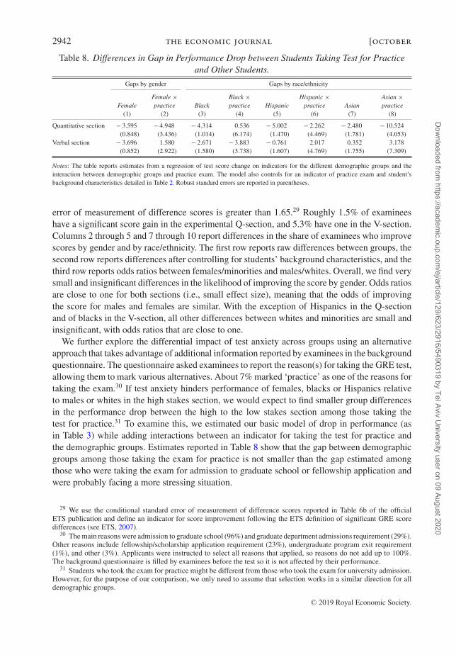
2942 the economic journal [october
Table 8. Differences in Gap in Performance Drop between Students Taking Test for Practiceand Other Students.
Gaps by gender Gaps by race/ethnicity
FemaleFemale ×practice Black
Black ×practice Hispanic
Hispanic ×practice Asian
Asian ×practice
(1) (2) (3) (4) (5) (6) (7) (8)
Quantitative section − 3.595 − 4.948 − 4.314 0.536 − 5.002 − 2.262 − 2.480 − 10.524(0.848) (3.436) (1.014) (6.174) (1.470) (4.469) (1.781) (4.053)
Verbal section − 3.696 1.580 − 2.671 − 3.883 − 0.761 2.017 0.352 3.178(0.852) (2.922) (1.580) (3.738) (1.607) (4.769) (1.755) (7.309)
Notes: The table reports estimates from a regression of test score change on indicators for the different demographic groups and theinteraction between demographic groups and practice exam. The model also controls for an indicator of practice exam and student’sbackground characteristics detailed in Table 2. Robust standard errors are reported in parentheses.
error of measurement of difference scores is greater than 1.65.29 Roughly 1.5% of examineeshave a significant score gain in the experimental Q-section, and 5.3% have one in the V-section.Columns 2 through 5 and 7 through 10 report differences in the share of examinees who improvescores by gender and by race/ethnicity. The first row reports raw differences between groups, thesecond row reports differences after controlling for students’ background characteristics, and thethird row reports odds ratios between females/minorities and males/whites. Overall, we find verysmall and insignificant differences in the likelihood of improving the score by gender. Odds ratiosare close to one for both sections (i.e., small effect size), meaning that the odds of improvingthe score for males and females are similar. With the exception of Hispanics in the Q-sectionand of blacks in the V-section, all other differences between whites and minorities are small andinsignificant, with odds ratios that are close to one.
We further explore the differential impact of test anxiety across groups using an alternativeapproach that takes advantage of additional information reported by examinees in the backgroundquestionnaire. The questionnaire asked examinees to report the reason(s) for taking the GRE test,allowing them to mark various alternatives. About 7% marked ‘practice’ as one of the reasons fortaking the exam.30 If test anxiety hinders performance of females, blacks or Hispanics relativeto males or whites in the high stakes section, we would expect to find smaller group differencesin the performance drop between the high to the low stakes section among those taking thetest for practice.31 To examine this, we estimated our basic model of drop in performance (asin Table 3) while adding interactions between an indicator for taking the test for practice andthe demographic groups. Estimates reported in Table 8 show that the gap between demographicgroups among those taking the exam for practice is not smaller than the gap estimated amongthose who were taking the exam for admission to graduate school or fellowship application andwere probably facing a more stressing situation.
29 We use the conditional standard error of measurement of difference scores reported in Table 6b of the officialETS publication and define an indicator for score improvement following the ETS definition of significant GRE scoredifferences (see ETS, 2007).
30 The main reasons were admission to graduate school (96%) and graduate department admissions requirement (29%).Other reasons include fellowship/scholarship application requirement (23%), undergraduate program exit requirement(1%), and other (3%). Applicants were instructed to select all reasons that applied, so reasons do not add up to 100%.The background questionnaire is filled by examinees before the test so it is not affected by their performance.
31 Students who took the exam for practice might be different from those who took the exam for university admission.However, for the purpose of our comparison, we only need to assume that selection works in a similar direction for alldemographic groups.
C© 2019 Royal Economic Society.
Dow
nloaded from https://academ
ic.oup.com/ej/article/129/623/2916/5490319 by Tel Aviv U
niversity user on 09 August 2020
2019] performance in high vs. low stakes tests 2943
Taken together, the evidence presented in Tables 7 and 8 suggests that test anxiety in the highstakes section is unlikely to be the reason for the smaller change in performance between thehigh and the low stakes tests observed among females and minorities.
4.3. Other Explanations
An additional explanation for our results could be that the monetary prize offered to experimentparticipants had a differential impact on different demographic groups. While this is possible, wenote that the prize consisted of $250 (1.5 times the GRE cost) paid to 100 individuals out of 30,000experiment participants. Such an amount distributed to such a small number of participants seemstoo low to have a significant differential effect in performance. Alternatively, it is arguably thecase that differences in performance in the experimental section arise from group differences intheir opportunity cost of time. However, as shown in Table 1, participation rates in the experimentwere similar across demographic groups, suggesting that there were no group differences in theperceived cost or benefit of participating in the experiment.
To further assess the impact of the monetary prize and the opportunity cost of time onperformance in the experimental section, we examined the association between the change inperformance (from the high to the low stakes section) and earning levels in the state of residenceof the examinee. We use two measures of earnings: median annual earnings of full-time workersand median annual earnings of college graduates computed separately by gender and state.32
If the monetary prize or the opportunity cost of time had any impact on performance in theexperimental section, we should expect a smaller reduction in performance in states with lowerearnings levels. In Appendix Table A7 we report regression estimates for the association betweenthe change in performance and median earnings for males and females. Columns 1 and 3 reportestimates from simple bivariate models and columns 2 and 4 report estimates from regressionsthat control for examinee characteristics. Overall, we do not find any association between medianearnings in the state of residence of the examinee and his/her change in performance, suggestingthat our main results are unlikely to be explained by a differential impact of the monetary prizeor the opportunity cost of time.
Another alternative explanation for differential changes in performance could be that per-formance of females and minorities is lower than expected in the high stakes section owing tostereotype threat (e.g., Steel and Aronson, 1995; Steele, 1997). However, it is unclear why genderand race/ethnicity stereotypes would be more pronounced in the high stakes section. In addition,the fact that we find similar gender differences in both the quantitative and the verbal sectionssuggests that stereotype threat is unlikely to explain our main results, as the theory would predictthat females would respond negatively only to the quantitative section. Moreover, stereotypethreat theory implies that Asians should respond differently than blacks and Hispanics in theQ-section, but our findings are similar for the three groups.
We further assess the likelihood of stereotype threat explanation by examining the relationshipbetween gender stereotypes in math and verbal achievement in the state of residence of theexaminees, and the differential change in performance. To proxy for gender stereotypes in thestate of residence of the examinee, we use the stereotype adherence index developed by Pope andSydnor (2010), which reflects gender disparities in test scores favouring boys in math and scienceand favouring girls in reading and which was shown by the authors to be positively associated
32 Earnings come from data published by the U.S. Census Bureau based on 5-year average earnings by state andgender from American Community Survey for the years 2005–2008.
C© 2019 Royal Economic Society.
Dow
nloaded from https://academ
ic.oup.com/ej/article/129/623/2916/5490319 by Tel Aviv U
niversity user on 09 August 2020
2944 the economic journal [october
with other measures of gender stereotype attitudes at the state level.33 Higher values in thisindex mean a stronger gender stereotype. To facilitate interpretation of the results, we transformthis index into a z-score. We hypothesize that stereotype threat plays a more important role instates with higher values in the stereotype index. Therefore, for our results to be consistent withstereotype threat, we should observe a larger gender differential in the Q-section and a smallergender differential in the V-section in states with a higher stereotype index. In Appendix TableA6, we examine this hypothesis by regressing the score difference between the high and the lowstakes section on a female indicator, the gender stereotype index and an interaction between thesetwo variables. Estimates for the interaction term between female and the stereotype index areall small and insignificant, meaning that there is no apparent relationship between state genderstereotypes and the gender gap in differential performance between the high and the low stakessection. Moreover, the estimates’ sign goes in the opposite direction than would be expected bythe stereotype threat theory.
An additional alternative interpretation of our findings could be that group differences inunderlying ability might generate a differential drop in performance. However, as we note above,we observe the same pattern of gender and racial/ethnic differences across different subsamplesand even in subsamples that exhibit similar performance in the high or the low stakes section.
It could also be the case that females and minorities become less fatigued by the GRE examina-tion than males and whites, respectively, and therefore exhibit a smaller drop in performance in theexperimental section. This argument seems unlikely as it goes against recent psychological andmedical literature that claims that, if anything, females appear to exhibit a higher level of fatigueafter performance of cognitive tasks (see, e.g., Yoon et al., 2009). In addition, we are not awareof any studies that show that whites exhibit a higher level of fatigue in response to cognitive taskscompared with blacks, Hispanics, or Asians. Furthermore, in the context of aptitude tests, Acker-man and Kanfer (2009) and Liu et al. (2004) show no evidence for a decline in test performancein the longer test conditions. Moreover, the fact that we find similar participation rates in theexperiment among males and females and whites, blacks, Hispanics and Asians provides furtherevidence that a differential effect of fatigue is unlikely to explain our findings. Lastly, as shown inAppendix Table A4, the fact that we can replicate our results in the samples of students randomisedinto the extended time-limit sections provides strong evidence that mitigates this concern.34
One could argue that group differences in performance change between the low and the highstakes section can be explained by differences in learning or test familiarisation. To assessthis conjecture, we took advantage of one additional piece of information at our disposal. Thebackground questionnaire collected information on examinees’ preparation methods for the GREexam (e.g., use of software or books published by the Educational Testing Service (ETS) or otherproviders, coaching courses offered by commercial companies, coaching courses offered byeducational institutions, no preparation, etc.). We coded this information in a vector of dummyvariables and re-estimated our main models while controlling for these additional covariates.
33 Pope and Sydnor (2010) use test-score data from the National Assessment of Educational Progress (NAEP) andshow that states that have larger gender disparities in stereotypically male-dominated tests of math and science also tendto have larger gender disparities (of the opposite sign) in stereotypically female-dominated tests of reading. The authorsdevelop a state stereotype adherence index that is defined as the average of the male–female ratio in math and scienceand female–male ratio in reading for the top 5% of the students.
34 Cotton et al. (2013) find that the advantage of males over females erodes over a sequence of quizzes of equalimportance. However, they note that this cannot be attributed to differential fatigue because the effect was also foundwhen there was a two-week gap between the different quizzes. In fact, they interpret their result by claiming that malesseem to become less excited about the quizzes over time, which lowers the stakes of these quizzes. This interpretationisthus consistent with our findings.
C© 2019 Royal Economic Society.
Dow
nloaded from https://academ
ic.oup.com/ej/article/129/623/2916/5490319 by Tel Aviv U
niversity user on 09 August 2020
2019] performance in high vs. low stakes tests 2945
Results of these expanded models are reported in Appendix Table A7, together with resultsfrom our main specification. All estimates are highly similar to our main results, suggesting thatlearning or test familiarisation cannot explain our findings.
Finally, our results might also be explained by the fact that some groups might get ‘bored’faster than others, and this might harm their performance. This would imply that there aregroup differences in the likelihood of getting bored when incentives are low. We believe that theimplications of our results are still relevant under this alternative interpretation.
4.4. Relation to Other Assessment Tests
Our findings demonstrate that test-score gaps between males and females or between whitesand minorities might vary according to the stakes of the test, as each group appears to responddifferently to level of stakes. Therefore, it is important to consider the stakes of a test and thedifferential performance of each group according to the stakes level when analysing test-scoregaps. We show this in Appendix Table A8, where we compare the (low stakes) National Assesmentof Educational Progress (NAEP) test scores in mathematics achieved by 12th-grade students in2015 to the (high stakes) Scholastic Aptitude Test (SAT) scores in 2015. Consistent with ourresults, we see that test-score gaps between males and females, and whites and blacks, whites andHispanics, and whites and Asians are larger for the SAT compared with the NAEP. While manyexplanations are offered for the differences in performance in SAT and NAEP exams, resultsfrom our study imply that males might just exert lower effort in NAEP exams. This is supportedby Freund and Rock’s (1992) finding of a higher prevalence of pattern-marking behaviour amongmales in the NAEP exam, which they interpret as an attempt to complete the exam as quickly andwith as little effort as possible. Similar gender differences in response patterns were also foundby Chiacchio et al. (2016), who analysed students’ responses for the Italian Pisa Science exam of2006. Our results are also consistent with the claim that standardised tests usually underpredictcollege and graduate school performance for women and overpredict performance for men (see,e.g., Willingham and Cole, 1997; Rothstein, 2004).35
4.5. Nature or Nurture
It is interesting to try to determine to what extent differences in performance between high andlow stakes situations are socially constructed or innate.36 While this question is beyond the scopeof the current study, we speculate that the similarity between Asian males and females suggeststhat part of the source for the gender differences observed among other ethnic and racial groupsmight be explained by acquired rather than innate skills. Women are generally perceived asmore conscientious and/or altruistic than men.37 Other possible explanations may be associatedwith experimenter demand effects and/or with higher salience of the reward for women andnon-whites.
35 Our findings also suggest the same pattern for whites compared with minorities, but this is not the case in practice(see, e.g., Mattern et al., 2008), presumably because the lower performance of minority students in college can beexplained by other factors such as their relatively disadvantaged background (Rothstein, 2004).
36 See, e.g., Gneezy et al. (2009), Booth and Nolen (2011,2012).37 Interestingly, these stereotypes do not have firm empirical support. In a recent review of various meta-analyses,
Hyde (2014) finds only small or no gender differences in the Big Five personality traits. The only exception is a higherscore of women on ‘tender-mindedness’, which is part of the agreeableness factor (Cohen’s d between 0.3 and 1.07 forU.S. and Japanese adults, but not for black South Africans).
C© 2019 Royal Economic Society.
Dow
nloaded from https://academ
ic.oup.com/ej/article/129/623/2916/5490319 by Tel Aviv U
niversity user on 09 August 2020
2946 the economic journal [october
Fig. 8. Performance Gap between High and Low Stakes Test by Undergraduate Major: QuantitativeSection.
Notes: The figure plots the performance gap between the high and the low stakes Q-section by subjects’undergraduate major. We include only majors that have at least 30 observations. Test scores are measuredin percentile score ranks.
A curious finding that relates to this question is presented in Figure 8, where we plot differencesin achievement between the high and the low stakes Q-section by students’ undergraduate major.Interestingly, those who exhibit the largest gap in achievement between the high and the low stakessection are economics majors. This finding could be a result either of self-selection into economicmajors or of skills acquired during undergraduate studies. Be that as it may, it is consistent withRubinstein (2006), who finds that economics majors have a much stronger tendency to maximiseprofits relative to other undergraduate majors.
5. Conclusions
In this study, we examined the change in performance of females, males, whites and minoritiesbetween high and low stakes situations by comparing the performance of GRE examinees in thereal and in an experimental section of the test. Our results show that males and whites have thehighest change in performance relative to females, Asians, Hispanics and blacks. Males’ drop inperformance between the high and low stakes section is 0.16 SD larger than the drop of females;whites’ drop in performance in the Q-section is 0.23 SD larger than the drop of blacks and thedrop of Hispanics, and 0.19 SD larger than the drop of Asians. We showed that the larger changein performance observed among males and whites is partially due to the fact that these two groupsinvest less effort in the low stakes test. We ruled out alternative explanations for these findings,such as stereotype threat, differences in stress levels, learning or alternative cost of time.
C© 2019 Royal Economic Society.
Dow
nloaded from https://academ
ic.oup.com/ej/article/129/623/2916/5490319 by Tel Aviv U
niversity user on 09 August 2020
2019] performance in high vs. low stakes tests 2947
Our findings suggest that men and whites who perform well in high stakes tests might notperform as well in ordinary assignments, and that women and minorities who do not performso well in high stakes tests may do relatively better in low stakes tasks. Accordingly, our resultsmay have implications for admission policies that are intended to achieve demographic diversityin educational institutions and the workplace. If different groups perform differently in low andhigh stakes situations, then policymakers may be able to diversify the population admitted tocolleges, universities, specific study fields and workplaces by putting more weight on ‘low stakes’measures of achievement and performance, such as high school performance and grades, extra-curricular activities, and recommendation letters (as opposed to focusing entirely on performancein standardised tests).
Finally, our results may also have implications for personnel and incentive policies, as theysuggest that differences in productivity between workers could vary according to the incentivescheme attached to the job. Oftentimes, job candidates are evaluated using high stakes tests.However, most jobs require excellence in tasks that are not directly attached to high-poweredincentive schemes. This suggests that consideration of performance in high stakes tests should notcome at the expense of consideration of other indicators of ability that reflect good performancein low stakes situations.
Tel Aviv UniversityTel Aviv UniversityEducational Testing Service
Additional Supporting Information may be found in the online version of this article:
Online Appendix A.
ReferencesAckerman, P.L. and Knafer, R. (2009). ‘Test length and cognitive fatigue: an empirical examination of effects of
performance and Test-Taker reactions’, Journal of Experimental Psychology: Applied, vol. 15(2), pp. 163–81.Ariely, D., Gneezy, U. and Loewenstein, G. (2009). ‘Large stakes and big mistakes’, Review of Economic Studies, vol.
76(2), pp. 451–69.Azmat, G. and Petrongolo, B. (2014). ‘Gender and the labor market: What have we learned from field and lab experi-
ments?’, Labour Economics, vol. 30, pp. 32–40.Azmat, G., Bagues, M., Cabrales, A. and Iriberri, N. (2019). ’What you don’t know ... can’t hurt you? A natural field
experiment on relative performance feedback in higher education’, Management Science, vol. 65:3449–3497.Babcock, L., Recalde, M.P., Vesterlund, L. and Weingart, L. (2017). ‘Gender differences in accepting and receiving
requests for tasks with low promotability’, American Economic Review, vol. 107(3), pp. 714–47.Booth, A. and Nolen, P. (2011). ‘Choosing to compete: How different are girls and boys?’, Journal of Economic Behaviour
and Organization, vol. 81 (2), pp. 542–555.Booth, A. and Nolen, P. (2012). ‘Gender differences in risk behaviour: Does nurture matter?’, Economic Journal, 122
(558), pp. F56–F78.Borghans L., , Meijers , H. and Weel, B.T. (2008). ‘The role of noncognitive skills in explaining cognitive test scores’,
Economic Inquiry, vol. 46(1), pp. 2–12.Bridgeman, B., Cline, F. and Hessinger, J. (2004). ‘Effect of extra time on verbal and quantitative GRE scores’, Journal
of Applied Measurement in Education, vol. 17(1), pp. 25–37.Cassaday, J.C. and Johnson, R.E. (2002). ‘Cognitive test anxiety and academic performance’, Contemporary Educational
Psychology, vol. 27(2), pp. 270–95.Chiacchio, C., De Stasio, S. and Fiorilli, C. (2016). ‘Examining how motivation towards science contributes to omitting
behaviors in the Italian PISA 2006 sample, Learning and Individual Differences, vol. 50, pp. 56–63.Cole, J.S., Bergin, D.A. and Whittaker, T.A. (2008). ‘Predicting student achievement for low stakes test with effort and
task value’, Contemporary Educational Psychology, vol. 33(4), pp. 609–24.Cotton, C., McIntyre, F. and Price, J. (2013). ‘Gender differences in repeated competition: evidence from school math
contests’, Journal of Economic Behaviour and Organization, vol. 86.
C© 2019 Royal Economic Society.
Dow
nloaded from https://academ
ic.oup.com/ej/article/129/623/2916/5490319 by Tel Aviv U
niversity user on 09 August 2020
2948 the economic journal [october
Cribbie, R.A. and Jamieson, J. (2000). ‘Structural equation and the regression bias for measuring correlates of change’,Educational and Psychological Measurement, vol. 60(6), pp. 893–907.
Croson, R. and Gneezy, U. (2009). ‘Gender differences in preferences’, Journal of Economic Literature, vol. 47(2), pp.448–74.
Cunha, F. and Heckman, J.J. (2007). ‘The technology of skill formation’, American Economic Review, vol. 97(2), pp.31–47.
Datta Gupta, N., Poulsen, A. and Villeval, M.C. (2005). ‘Male and female competitive behaviour: experimental evidence’,IZA Discussion Paper No. 1833, IZA institute of Labor Economics.
Dohmen, T.J. and Falk, A. (2011). ‘Performance pay and multi-dimensional sorting: productivity, preferences, andgender’, American Economic Review, vol. 101(2), pp. 493–525.
Duckworth, A.L. and Seligman, M.E.P. (2006). ‘Self-discipline gives girls the edge: gender in self-discipline, grades,and achievement test scores’, Journal of Educational Psychology, vol. 98(1), pp. 198–208.
Educational Testing Service.(2007). Graduate Record Examinations, Guide to the Use of Scores 2007-2008.Flory, J.A., Leibbrandt, A. and List, J.A. (2010). ‘Do competitive work places deter female workers? A large-scale natural
experiment on gender differences in job entry decisions’, NBER Working Paper No. 16546.Freund, D.S. and Rock, D.A. (1992). ‘A preliminary investigation of pattern-making in 1990 NAEP data’, paper presented
at the Annual Meeting of the American Educational Research Association (San Francisco, CA, April 20–24).Retrieved from ERIC Document Reproduction Service. (ED 347189)
Gneezy, U., Leonard, K.L. and List, J.A. (2009). ‘Gender differences in competition: evidence from a matrilineal and apatriarchal society’, Econometrica,vol. 77(5), pp. 1637–64.
Gneezy, U., Niederle, M. and Rustichini, A. (2003). ‘Performance in competitive environments: gender differences’,Quarterly Journal of Economics, vol. 108(3), pp. 1049–74.
Gneezy, U. and Rustichini, A. (2004). ‘Gender and competition at a young age’, American Economic Review Papers andProceedings, vol. 94(2), pp. 377–81.
Heckman, J.J. and Rubinstein, Y. (2001). ‘The importance of noncognitive skills: lessons from the GED testing program’,American Economic Review Papers and Proceedings, vol. 91(2), pp. 145–9.
Hyde, J.S. (2014). ‘Gender similarities and differences’, Annual Review of Psychology, vol. 65, pp. 373–98.Jurajda, S. and Munich, D. (2011). ‘Gender gap in admission performance under competitive pressure’, American
Economic Review Papers and Proceedings, 101 (3), pp. 514–518, May.Lavy, V. (2008). ‘Gender differences in competitiveness in a real workplace: evidence from performance-based pay
tournaments among teachers’, NBER Working Paper 14338.Levitt, S.D., List, J. and Sadoff, S. (2016). ‘The effect of performance-based incentives on educational achievement:
evidence from a randomised experiment’, NBER Working Paper 22107.Liu, J., Allspach, J.R., Feigenbaum, M., Oh, H.J. and Burton, N. (2004). ‘A study of fatigue effects from the new SAT’,
College Board Research Report No. 2004–2005, The College Board, New York.Lord, F.M. (1967). ‘A paradox in the interpretation of group comparisons’, Psychological Bulletin, vol. 68(5), pp. 304–5.Mattern, K.D., Patterson, B.F., Shaw, E.J., Kobrin, J.L. and Barbuti, S.M. (2008). ‘Differential validity and prediction of
the SAT’, College Board Research Report No. 2008–4, The College Board, New York.Niederle, M. (2016). ‘Gender’, in (J. Kagel and A.E. Roth, eds.), Handbook of Experimental Economics, 2nd edition, pp.
481–553, Princeton, NJ: Princeton University Press.Niederle, M. and Vesterlund, L. (2007). ‘Do women shy away from competition? Do men compete too much?’, Quarterly
Journal of Economics, vol. 122(3), pp. 1067–101.O’Neil, H.F., Sugrue, B. and Baker, E.L. (1996). ‘Effects of motivational interventions on the national assessment of
educational progress mathematics performance’, Educational Assessment, vol. 2(2), pp. 135–57.Ors, E., Palomino, F. and Peyrache, E. (2008). ‘Performance gender-gap: Does competition matter?’, CEPR Discussion
Paper No. 6891.Paserman, D. (2010). ‘Gender differences in performance in competitive environments: evidence from professional tennis
players’, Discussion Paper, Boston University.Pope, D.G. and Sydnor, J.R. (2010). ‘Geographic variation in the gender differences in test scores’, Journal of Economic
Perspectives, vol. 24(2), pp. 95–108.Rothstein, J. (2004). ‘College performance predictions and the SAT’, Journal of Econometrics, vol. 121(1-2), pp. 123–44.Rubinstein, A. (2006). ‘A skeptic’s comment on the study of economics’, ECONOMIC JOURNAL, vol. 116(510), pp. C1–C9.Segal, C. (2010). ‘Motivation, test scores, and economic success’, Working Paper, Universitat Pompeu Fabra.Spencer, S., Steele, C.M. and Quinn, D.M. (1999). ‘Stereotype threat and women’s math performance’, Journal of
Experimental Social Psychology, vol. 35(1), pp. 4–28.Steele, C.M. (1997). ‘A threat in the air: how stereotypes shape the intellectual identities and performance of women and
African-Americans’, American Psychologist, vol. 52(6), pp. 613–29.Steele, C.M. and Aronson, J. (1995). ‘Stereotype threat and the intellectual test performance of African Americans’,
Journal of Personality and Social Psychology, vol. 69(5), pp. 797–811.Willingham, W.W. and Cole, N.S. (1997). Gender and Fair assessment, Mahwah, NJ: Erlbaum.Yoon, T., Keller, M., Schinder De-Lap, B., Harkins, A., Lepers, R. and Hunter, S. (2009). ‘Sex differences in response to
cognitive stress during a fatiguing contraction’, Journal of Applied Physiology, vol. 107(5), pp. 1486–96.
C© 2019 Royal Economic Society.
Dow
nloaded from https://academ
ic.oup.com/ej/article/129/623/2916/5490319 by Tel Aviv U
niversity user on 09 August 2020
Online appendix
Total Males Females Missing Whites Blacks Hispanics AsiansOther/Missing
Population (all GRE tested 9/1/2001‐10/31/2001) 81,231 34,723 41,617 4,891US citizens tested in the US 46,038 15,749 30,160 129 36,042 2,877 2,400 2,584 2,135
Experiment participants (total) 29,962 13,359 14,803 1,800 US citizens tested in the US 15,945 5,486 10,458 1 12,374 1,024 850 982 715
Participants in regular time limit experiment 8,232 2,834 5,398 0 6,407 513 445 479 388Participants in Q section 3,922 1,369 2,553 3,027 265 224 224 182Participants in V section 4,310 1,465 2,845 3,380 248 221 255 206
Gender Race/ethnicityTable A1. Sample Construction Process
Notes: The table reports the process we followed to select our analysis samples.
Online appendix
Males Females Whites Blacks Hispanics Asians(1) (2) (3) (4) (5) (6)
Females 0.66 0.74 0.65 0.63Race/Ethnicity
Whites 0.78 0.78Blacks 0.05 0.07Hispanics 0.06 0.05Asians 0.06 0.06American Indian or Alaskan Native 0.00 0.01Other 0.05 0.04
Mother's EducationHigh School or less 0.23 0.22 0.21 0.33 0.40 0.24College or some college 0.45 0.48 0.48 0.41 0.37 0.46At least some graduate studies or professional degree 0.26 0.25 0.26 0.19 0.19 0.25Missing 0.06 0.05 0.04 0.07 0.04 0.05
Father's EducationHigh School or less 0.21 0.23 0.20 0.43 0.40 0.15College or some college 0.40 0.44 0.44 0.38 0.33 0.39At least some graduate studies or professional degree 0.37 0.32 0.35 0.16 0.25 0.45Missing 0.01 0.01 0.01 0.04 0.02 0.01
Native English speaker 0.93 0.92 0.93 0.95 0.90 0.86Undergraduate GPA
C or C‐ 0.07 0.05 0.05 0.20 0.08 0.05B‐ 0.11 0.10 0.10 0.18 0.13 0.07B 0.30 0.33 0.32 0.36 0.37 0.36A‐ 0.28 0.28 0.30 0.13 0.23 0.30A 0.19 0.19 0.21 0.07 0.13 0.18Missing 0.04 0.04 0.03 0.06 0.07 0.05
Undergraduate major in Physics, Math, Comp. Science or Engineering 0.26 0.05 0.12 0.10 0.12 0.31Grad. intended studies in Physics, Math, Comp. Science or Engineering 0.25 0.05 0.11 0.07 0.13 0.30
Table A2. Descriptive Statistics of Experiment Participants
Notes: The table reports descriptive statistics of participants in the regular time limit experiment. The samples are restricted to US citizens tested in the US.
Online appendix
Males Females Whites Blacks Hispanics AsiansMales‐Females
Whites‐Blacks
Whites‐Hispanics
Whites‐Asians
(1) (2) (3) (4) (5) (6) (7) (8) (9) (10)
Raw scores 76.952 51.324 65.601 21.019 32.321 43.616 23.018 32.553 31.455 26.256(4.402) (2.596) (2.650) (6.085) (8.818) (9.464) (5.414) (7.288) (9.187) (10.395)
Ln(raw scores) 0.182 0.130 0.161 0.054 0.091 0.098 0.048 0.083 0.067 0.072(0.011) (0.007) (0.007) (0.016) (0.022) (0.022) (0.013) (0.019) (0.023) (0.024)
Standardized scores 0.551 0.367 0.469 0.150 0.231 0.312 0.165 0.233 0.225 0.188(z‐scores) (0.031) (0.019) (0.019) (0.044) (0.063) (0.068) (0.039) (0.052) (0.066) (0.074)
Percentile score ranks 11.560 6.330 8.708 1.585 3.995 10.573 4.251 5.081 3.440 ‐0.901Extended time limit sample (0.733) (0.421) (0.421) (1.071) (1.611) (1.789) (0.931) (1.203) (1.741) (1.847)
Percentile score excluding 4.636 2.124 3.590 ‐0.370 ‐1.615 0.622 3.133 4.315 5.479 2.365largest drop in performance (0.407) (0.247) (0.245) (0.516) (0.772) (0.868) (0.533) (0.643) (0.839) (0.944)
Raw scores 45.993 26.882 34.275 11.935 27.059 39.255 15.658 11.646 4.293 ‐1.577(3.022) (1.748) (1.734) (5.779) (6.118) (7.073) (3.626) (6.442) (6.480) (7.391)
Ln(raw scores) 0.121 0.072 0.091 0.037 0.072 0.103 0.041 0.029 0.013 ‐0.004(0.008) (0.005) (0.005) (0.016) (0.016) (0.018) (0.009) (0.017) (0.017) (0.019)
Standardized scores 0.430 0.251 0.320 0.112 0.253 0.367 0.146 0.109 0.040 ‐0.015(z‐scores) (0.028) (0.016) (0.016) (0.054) (0.057) (0.066) (0.034) (0.060) (0.061) (0.069)
Percentile score ranks 11.380 4.575 7.428 1.240 3.894 8.008 5.781 3.364 2.347 0.181Extended time limit sample (0.748) (0.413) (0.423) (1.101) (1.539) (1.814) (0.895) (1.261) (1.612) (1.844)Percentile score excluding 3.473 0.699 1.682 ‐3.151 1.015 2.052 2.873 4.330 0.656 ‐0.386largest drop in performance (0.420) (0.260) (0.242) (0.857) (1.053) (1.021) (0.539) (0.950) (1.086) (1.080)
Notes: The table reports differences in performance between the high and the low stakes tests by gender and race/ethnicity and the controlled differencebetween males and females or whites and minorities. The first row of each panel uses difference in raw test scores as a dependent variable. The second row usesdifference in the natural logarithm of raw scores as a dependent variable. The third row uses differences in standardized scores (z‐scores). The third row usesdifference in percentile score ranks (as all our main results table) based on the sample of students who got the experimental GRE section with an extended timelimit. The last row excludes from our main sample students in the top 10 percentile drop in performance of each demographic group. Standard deviations androbust standard errors are reported in parenthesis.
Table A3. Robustness Check: Differential Performance in High versus Low Stakes Tests
Difference in performance between high and low stake test Controlled difference between groups
A. Quantitative Section
B. Verbal Section
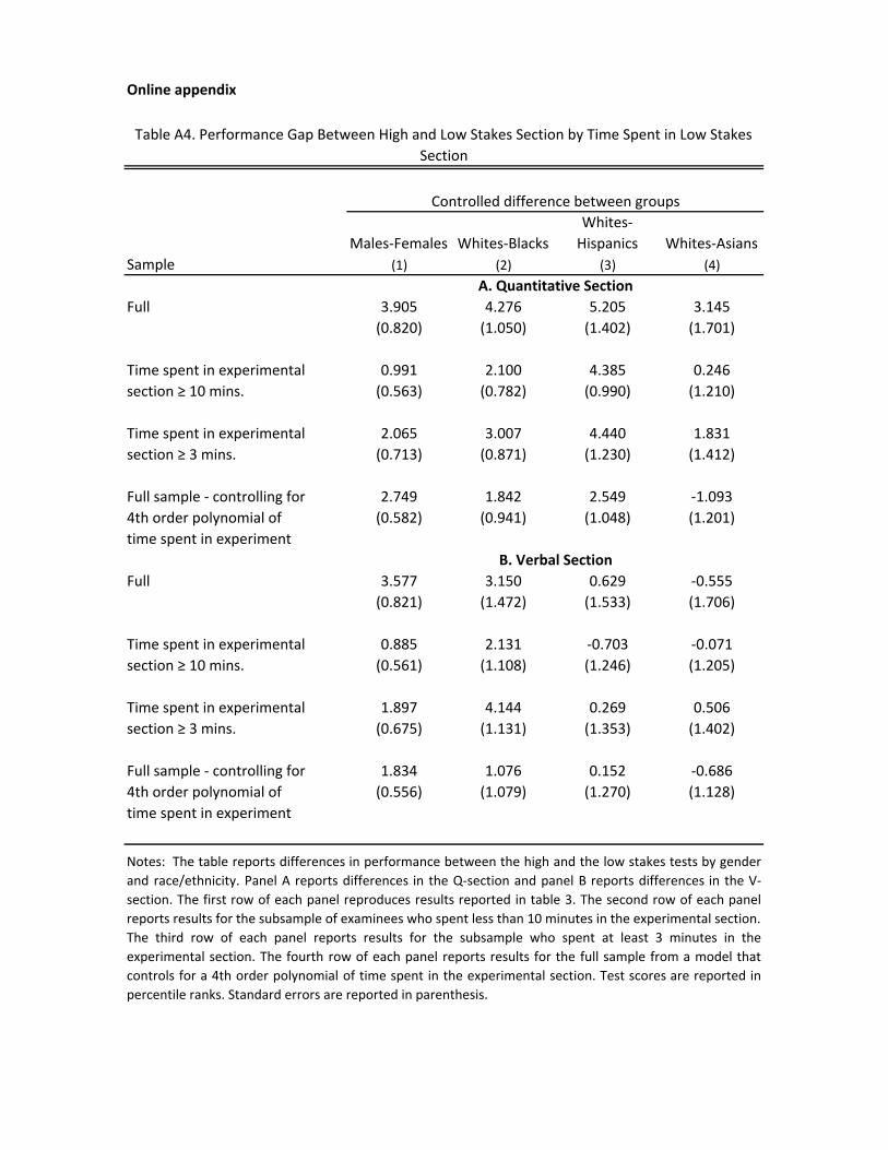
Online appendix
Males‐Females Whites‐BlacksWhites‐Hispanics Whites‐Asians
Sample (1) (2) (3) (4)
Full 3.905 4.276 5.205 3.145(0.820) (1.050) (1.402) (1.701)
0.991 2.100 4.385 0.246(0.563) (0.782) (0.990) (1.210)
2.065 3.007 4.440 1.831(0.713) (0.871) (1.230) (1.412)
Full sample ‐ controlling for 2.749 1.842 2.549 ‐1.0934th order polynomial of (0.582) (0.941) (1.048) (1.201)time spent in experiment
Full 3.577 3.150 0.629 ‐0.555(0.821) (1.472) (1.533) (1.706)
0.885 2.131 ‐0.703 ‐0.071(0.561) (1.108) (1.246) (1.205)
1.897 4.144 0.269 0.506(0.675) (1.131) (1.353) (1.402)
Full sample ‐ controlling for 1.834 1.076 0.152 ‐0.6864th order polynomial of (0.556) (1.079) (1.270) (1.128)time spent in experiment
Notes: The table reports differences in performance between the high and the low stakes tests by genderand race/ethnicity. Panel A reports differences in the Q‐section and panel B reports differences in the V‐section. The first row of each panel reproduces results reported in table 3. The second row of each panelreports results for the subsample of examinees who spent less than 10 minutes in the experimental section. The third row of each panel reports results for the subsample who spent at least 3 minutes in theexperimental section. The fourth row of each panel reports results for the full sample from a model thatcontrols for a 4th order polynomial of time spent in the experimental section. Test scores are reported inpercentile ranks. Standard errors are reported in parenthesis.
Time spent in experimental section ≥ 10 mins.
Time spent in experimental section ≥ 10 mins.
Table A4. Performance Gap Between High and Low Stakes Section by Time Spent in Low Stakes Section
Controlled difference between groups
Time spent in experimental section ≥ 3 mins.
Time spent in experimental section ≥ 3 mins.
B. Verbal Section
A. Quantitative Section
Online appendix
(1) (2) (3) (4)
Median earnings ‐0.169 ‐0.221 0.124 0.059(in thousand dollars) (0.161) (0.182) (0.130) (0.142)
Median earnings of college 0.049 0.083 0.012 ‐0.036graduates (in thousand dollars) (0.151) (0.151) (0.143) (0.142)
Median earnings 0.211 0.089 0.158 0.089(in thousand dollars) (0.162) (0.178) (0.076) (0.075)
Median earnings of college 0.191 0.131 0.109 0.045graduates (in thousand dollars) (0.111) (0.132) (0.112) (0.106)
Controls for examinee's covariates ‐‐ ‐‐
Table A5. Associations Between Median Earnings at the Examinee State of Residence and Differential Performance
Notes: The table reports regression estimates for the coefficient of annual median earnings (in thousand US$) offull time workers or college graduates working full time at the state of residence of the examinee. Thedependent variable is the score difference (in percentile points) between the high and the low stakes section.Estimates reported in columns (2) and (4) come from regressions that control for race/ethnicity, mother’s andfather’s education, dummies for UGPA, undergraduate major, intended graduate field of studies, and disabilitystatus. Standard errors clustered at the state levels are reported in parenthesis.
B. Verbal Section
Females
A. Quantitative Section
Males
Online appendix
(1) (2) (3) (4)
Female ‐4.434 ‐3.745 ‐4.851 ‐4.136(0.692) (0.879) (0.749) (0.863)
State stereotype index ‐1.108 ‐0.765 ‐0.149 ‐0.054(0.651) (0.645) (0.702) (0.657)
Female x State stereotype index 0.606 0.498 ‐0.796 ‐0.657(0.681) (0.747) (0.706) (0.712)
Controls for examinee's covariates ‐‐ ‐‐
Table A6. Differential Performance and Stereotype ThreatHigh Stakes ‐ Low Stakes
Quantitative Section Verbal Section
Notes: The table reports estimates from models that regress the score difference (in percentile points)between the high and the low stakes section on a female dummy, the gender stereotype index of thestate of residence of the examinee and the interaction between these two variables. Estimates reportedin columns (2) and (4) come from regressions that control also for race/ethnicity, mother’s and father’seducation, dummies for UGPA, undergraduate major, intended graduate field of studies, and disabilitystatus. The gender stereotype index was developed by Pope and Sydnor (2010) and reflects genderstereotypes in performance in math and science versus reading at the state level. Higher values denotestronger gender stereotypes. The index is standardized to have mean of 0 and a standard deviation of 1.Standard errors clustered at the state levels are reported in parenthesis.
Online appendix
Males‐Females
Whites‐Blacks
Whites‐Hispanics
Whites‐Asians
Males‐Females
Whites‐Blacks
Whites‐Hispanics
Whites‐Asians
(1) (2) (3) (4) (5) (6) (7) (8)
Basic specification 3.905 4.276 5.205 3.145 3.577 3.150 0.629 ‐0.555(0.820) (1.050) (1.402) (1.701) (0.821) (1.472) (1.533) (1.706)
3.959 4.019 5.216 3.496 3.746 3.402 0.793 ‐0.217(0.828) (1.065) (1.413) (1.683) (0.829) (1.468) (1.540) (1.707)
Table A7. Differential Gap Between High and Low Stakes Section After Controlling for Test Preparation MethodsVerbal Section
Notes: The table reports differences in performance between the high and the low stakes tests by gender and race/ethnicity. Columns 1‐4report differences in the Q‐section and columns 5‐8 report differences in the V‐section. The first row of the table reproduces estimates fromthe full specification reported in table 3. The second row reports results from regressions that control also for indicators for test preparationmethods reported by the examinees: no preparation, software from the ETS, books published by the ETS, software from other providers,books from other providers, attended a coaching course offered by a commercial company, attended a coaching course offered by aneducational institution, used ScoreItNow! online writing practice, used GRE enhanced diagnostic service, other type of preparation. Robuststandard errors are reported in parenthesis.
Quantitative Section
Controlling for test preparation methods
Online appendix
Males FemalesStandardized
mean difference Males FemalesStandardized
mean difference
Whites 161 159 0.063 551 518 0.320(33) (30) (107) (99)
Blacks 129 131 ‐0.065 435 422 0.130(31) (31) (104) (96)
Hispanics 141 136 0.156 473 443 0.456(33) (31) (70) (64)
Asian 171 169 0.056 611 585 0.207(36) (35) (125) (126)
Whites 290 301 ‐0.285 532 526 0.058(40) (37) (105) (101)
Blacks 259 272 ‐0.347 428 434 ‐0.060(38) (37) (102) (99)
Hispanics 272 279 ‐0.187 453 446 0.108(38) (37) (69) (67)
Asian 290 304 ‐0.354 525 526 ‐0.008(41) (38) (128) (124)
Table A8. Gender Gaps in Low and High Stakes Tests: NAEP vs. SAT Scores 2015
Notes: The table reports students' achievement in NAEP and SAT exams in 2015. The standardized meandifference (also known as effect size ‐ d ) is the average of men minus the average of women divided bythe within group standard deviations pooled across groups. Data for NAEP scores was downloaded fromthe National Centre for Education Statistics Website. Data from SAT scores come from SAT Total GroupProfile Report 2015 (College Board, 2015).
12th grade NAEP
A. Math
B. Reading
SAT