Embed Size (px)
Citation preview

Our reference: MATCOM 4028 P-authorquery-v9
AUTHOR QUERY FORM
Journal: MATCOM Please e-mail or fax your responses and any corrections to:
E-mail: [email protected]
Article Number: 4028 Fax: +353 6170 9272
Dear Author,
Please check your proof carefully and mark all corrections at the appropriate place in the proof (e.g., by using on-screenannotation in the PDF file) or compile them in a separate list. Note: if you opt to annotate the file with software other thanAdobe Reader then please also highlight the appropriate place in the PDF file. To ensure fast publication of your paper pleasereturn your corrections within 48 hours.
For correction or revision of any artwork, please consult http://www.elsevier.com/artworkinstructions.
Any queries or remarks that have arisen during the processing of your manuscript are listed below and highlighted by flags inthe proof. Click on the ‘Q’ link to go to the location in the proof.
Location in Query / Remark: click on the Q link to goarticle Please insert your reply or correction at the corresponding line in the proof
Q1 Please confirm that given names and surnames have been identified correctly.Q2 Please check the telephone number of the corresponding author, and correct if necessary.Q3 As per the stylesheet of this journal there should be a maximum of five keywords but in this article
more than five keywords are given. Please delete extra keyword.Q4 Please provide captions for Tables 1–5.
Please check this box or indicate your approval ifyou have no corrections to make to the PDF file
Thank you for your assistance.

Please cite this article in press as: L. Dieci, et al. Sharp sufficient attractivity conditions for sliding on a co-dimension 2discontinuity surface, Math. Comput. Simul. (2014), http://dx.doi.org/10.1016/j.matcom.2013.12.005
ARTICLE IN PRESS+ModelMATCOM 4028 1–12
Available online at www.sciencedirect.com
ScienceDirect
Mathematics and Computers in Simulation xxx (2014) xxx–xxx
Original Article
Sharp sufficient attractivity conditions for sliding on a co-dimension1
2 discontinuity surface�2
L. Dieci a, C. Elia b,∗, L. Lopez bQ13
a School of Mathematics, Georgia Tech, Atlanta, GA 30332, USA4
b Dipartimento di Matematica, Univ. of Bari, I-70100 Bari, Italy5
Received 26 March 2013; received in revised form 18 December 2013; accepted 19 December 2013
6
Abstract7
We consider Filippov sliding motion on a co-dimension 2 discontinuity surface. We give conditions under which Σ is attractive8
through sliding which are sharper than those given in a previous paper of ours. Under these sharper conditions, we show that9
the sliding vector field considered in the same paper is still uniquely defined and varies smoothly in x ∈ Σ. A numerical example10
illustrates our results.11
© 2014 IMACS. Published by Elsevier B.V. All rights reserved.12
13
Keywords: Piecewise smooth systems; Filippov systems; Sliding modes; Discontinuity surface; Co-dimension 2; AttractivityQ314
15
1. Introduction16
An outstanding problem in the study of piecewise smooth differential systems is how to properly define a Filippov17
sliding vector field when sliding motion has to take place on a co-dimension 2 surface, Σ, intersection of two co-18
dimension 1 surfaces. In [3], we gave sufficient conditions which guaranteed that Σ attracted nearby trajectories19
(through sliding), and that a certain sliding vector field, (7) below, was well defined on Σ. Our goal in this work is to20
sharpen the conditions given in [3], while still obtaining the same conclusions.21
The basic problem we consider is the piecewise smooth system22
x = f (x), f (x) = fi(x), x ∈ Ri, i = 1, . . ., 4, (1)23
with initial condition x(0) = x0 ∈ Ri, for some i. Here, the Ri ⊆ Rn are open, disjoint and connected sets, and (locally)24
Rn = ⋃
iRi. Each fi can be assumed smooth in an open neighborhood of the closure of each Ri, i = 1, . . ., 4. Clearly,25
from (1), the vector field is not properly defined on the boundaries of the Ri’s.26
Above, we will assume that the Ri’s are (locally) separated by two intersecting smooth surfaces of co-dimension 1,27
Σ1 = {x : h1(x) = 0} and Σ2 = {x : h2(x) = 0}, and we let Σ = Σ1 ∩ Σ2. We will always assume that ∇h1(x) /= 0, x ∈ Σ1,28
� This work was done while the second and third author were visiting the School of Mathematics of Georgia Institute of Technology, whosehospitality is gratefully acknowledged.
∗ Corresponding author. Tel.: +39 3333514208.Q2E-mail addresses: [email protected] (L. Dieci), [email protected], [email protected] (C. Elia), [email protected] (L. Lopez).
http://dx.doi.org/10.1016/j.matcom.2013.12.0050378-4754/© 2014 IMACS. Published by Elsevier B.V. All rights reserved.

Please cite this article in press as: L. Dieci, et al. Sharp sufficient attractivity conditions for sliding on a co-dimension 2discontinuity surface, Math. Comput. Simul. (2014), http://dx.doi.org/10.1016/j.matcom.2013.12.005
ARTICLE IN PRESS+ModelMATCOM 4028 1–12
2 L. Dieci et al. / Mathematics and Computers in Simulation xxx (2014) xxx–xxx
Fig. 1. Regions Ri’s, Σ and Σ±1,2.
∇h2(x) /= 0, x ∈ Σ2, that h1,2 are Ck functions, with k ≥ 2, and further that ∇h1(x) and ∇h2(x) are linearly independent29
for x on (and in a neighborhood of) Σ.30
Without loss of generality, we can label the regions as follows:31
R1 : f1 when h1 < 0, h2 < 0, R2 : f2 when h1 < 0, h2 > 0,
R3 : f3 when h1 > 0, h2 < 0, R4 : f4 when h1 > 0, h2 > 0,(2)32
and we will also adopt the notation Σ+1,2 and Σ−
1,2 to denote the set of points x ∈ Σ1,2 for which we also have h2,1(x) > 033
or h2,1(x) < 0. See Fig. 1.34
Finally, we let35
w11 = ∇hT
1 f1, w12 = ∇hT
1 f2, w13 = ∇hT
1 f3, w14 = ∇hT
1 f4,
w21 = ∇hT
2 f1, w22 = ∇hT
2 f2, w23 = ∇hT
2 f3, w24 = ∇hT
2 f4,(3)36
which we assume to be well defined in a neighborhood of Σ. As it turns out, the signs of the wij’s are the key property37
to monitor.38
Remark 1. Looking ahead, let us suppose that we are following a solution trajectory on Σ, x(t). In this case, we will39
need to consider the wij’s along this solution trajectory, and can thus think of the wi
j’s as functions of t.40
Remark 2. The classical Filippov theory (see [6]) is concerned with the case of two regions separated by a surface41
Σ defined as the 0-set of a smooth scalar valued function h:42
x = f1(x), x ∈ R1 = {x : h(x) < 0}, and x = f2(x), x ∈ R2 = {x : h(x) < 0},43
Σ := {x ∈ Rn : h(x) = 0}, h : Rn → R. (4)44
Filippov convexification method allows to define a sliding motion on Σ, in particular when Σ attracts nearby trajectories.45
Filippov proposal is to take a convex combination of f1 and f2 and impose that the vector field is tangent to Σ. That is,46
take fF : = (1 − α)f1 + αf2, with α chosen so that fF ∈ TΣ:47
x′ = (1 − α)f1 + αf2, α = w1
w1 − w2 , w1 = ∇h(x)T f1(x), w2 = ∇h(x)T f2(x). (5)48
With the above in mind, we can consider sliding on Σ±1,2 previously defined (if such sliding motion indeed can take49
place). According to (5), we will call fΣ±1,2
these four vector fields, defined as follows (as long as the denominators are50
nonzero):51

Please cite this article in press as: L. Dieci, et al. Sharp sufficient attractivity conditions for sliding on a co-dimension 2discontinuity surface, Math. Comput. Simul. (2014), http://dx.doi.org/10.1016/j.matcom.2013.12.005
ARTICLE IN PRESS+ModelMATCOM 4028 1–12
L. Dieci et al. / Mathematics and Computers in Simulation xxx (2014) xxx–xxx 3
52
fΣ+1
= (1 − α+)f2 + α+f4, fΣ−1
= (1 − α−)f1 + α−f3, fΣ+2
= (1 − β+)f3 + β+f4,53
fΣ−2
= (1 − β−)f1 + β−f2, and α+ = w12
w12 − w1
4
, α− = w11
w11 − w1
3
, β+ = w23
w23 − w2
4
,54
β− = w21
w21 − w2
2
. (6)55
56
2. Background57
When attempting to define a Filippov sliding vector field on Σ = Σ1 ∩ Σ2, one needs to consider a convex combi-58
nation of the four vector fields f1, . . ., f4 : fF = λ1f1 + λ2f2 + λ3f3 + λ4f4, λi ≥ 0, i = 1, . . ., 4, and∑
iλi = 1. Imposing that59
fF ∈ TΣ , however, is now no longer sufficient (unlike the case of Remark 2) to uniquely determine the coefficients λi’s.60
To resolve the above ambiguity, in [2,5,1] the authors proposed to restrict consideration to the following bilinear61
vector field62
fF = (1 − α)(1 − β)f1 + (1 − α)βf2 + α(1 − β)f3 + αβf4, (7)63
where now α, β ∈ [0, 1] need to be found so to satisfy the following nonlinear system:64
(1 − α)(1 − β)
[w1
1
w21
]+ (1 − α)β
[w1
2
w22
]+ α(1 − β)
[w1
3
w23
]+ αβ
[w1
4
w24
]= 0. (8)65
The question then becomes solvability (unique) of this system. To address this problem, in [3] we considered the case66
of Σ being reached through sliding on one of the Σ±1,2, and to characterize this situation we worked under the following67
assumptions.68
Assumptions 1.69
(a) (w1j (x), w2
j (x)) do not have the same signs as (h1(x), h2(x)) for x ∈ Rj, j = 1, 2, 3, 4.70
(b) At least one pair of the relations [(1+)and(1+a )], or [(1−)and(1−
a )], or [(2+)and(2+a )], or [(2−)and(2−
a )], is satisfied71
on Σ and in a neighborhood of Σ, where72
(1+)w12 > 0, w1
4 < 0, (1+a )
w22
w12
− w24
w14
< 0,
(1−)w11 > 0, w1
3 < 0, (1−a )
w23
w13
− w21
w11
< 0,
(2+)w23 > 0, w2
4 < 0, (2+a )
w13
w23
− w14
w24
< 0,
(2−)w21 > 0, w2
2 < 0, (2−a )
w12
w22
− w11
w21
< 0.
73
(c) If any of (1±) or (2±) is satisfied, then (1±a ) or (2±
a ) must be satisfied as well.74
Let us clarify the meaning of Assumptions 1 insofar as the dynamics of the system. Assumption 1(a) implies that the75
vector fields fj, j = 1, . . ., 4, must point toward at least one of Σ1,2. Assumption 1(b) guarantees that there is attractive76
sliding toward Σ along at least one of the Σ±1,2. Assumption 1(c) states that if attractive sliding occurs along Σ±
1,2 it77
must be toward Σ.78

Please cite this article in press as: L. Dieci, et al. Sharp sufficient attractivity conditions for sliding on a co-dimension 2discontinuity surface, Math. Comput. Simul. (2014), http://dx.doi.org/10.1016/j.matcom.2013.12.005
ARTICLE IN PRESS+ModelMATCOM 4028 1–12
4 L. Dieci et al. / Mathematics and Computers in Simulation xxx (2014) xxx–xxx
Fig. 2. Admissible f1 under the assumption w11(x) < 0.
It must be emphasized that our theory is justified under the assumption that Σ is attractive in finite time upon79
sliding on a co-dimension 1 surface. Hence, Assumption 1(c) are fundamental in this setting.80
In [3], we made a simplifying assumption on the wij’s, expressed by the following:81
Old assumption (see [3]):82
wij(x) areboundedawayfrom 0, i = 1, 2, j = 1, 2, 3, 4, x ∈ Σ. (9)83
Note that (9) implies that no trajectory can approach Σ tangentially from a region Rj, j = 1, 2, 3, 4.84
Under Assumptions 1 and (9), in [3] it was proved that Σ attracted nearby trajectories, which in fact reached Σ in85
finite time, and moreover that (8) had a unique solution. More precisely, we proved the following result.86
Theorem 3. Let Assumptions 1 be satisfied and let (9) hold.87
(a) Then, there exists a unique solution (α, β) of system (8) in (0, 1) × (0, 1).88
(b) Further, let (1+a ), (1−
a ), (2+a ), and (2−
a ), hold uniformly; that is (1+a ) be replaced by (w2
2/w12) − (w2
4/w14) ≤ −λ+
1 < 0,89
and similarly for the others. Then, Σ is attractive in finite time.90
3. Weaker attractivity assumptions91
It was already observed in [3] that (9) was too strong a sufficient condition to guarantee the conclusions of Theorem92
3. For this reason, our goal below is to weaken (9) in such a way that: Σ still remains attractive through sliding and93
reached in finite time, and the vector field (7) still is well defined on Σ.94
We restrict ourselves to co-dimension 1 phenomena, as characterized by having just one scalar value among the95
wij’s being 0 at any point in Σ. Higher co-dimension phenomena (such as two of the wi
j’s becoming 0 at the same96
time) are not necessarily going to preclude the aforementioned conclusions (i.e., attractivity of Σ and well posedness97
of the vector field (7)), but require a host of different possibilities to be examined, which is beyond our present scope.98
Assumptions 2. At most one of the wij’s is zero at any given x on Σ.99
In this paper we replace condition (9) with Assumptions 2. This means that, while sliding on Σ, one of the wij’s100
can be zero at a point x ∈ Σ, as long as Assumptions 1 are still satisfied.101
Assumptions 1 and 2 together imply the following:102
(i) fj cannot be tangential to Σ at x ∈ Σ;103
(ii) fj cannot be tangential to Σ2 (respectively, Σ1), at a point x on Σ, whenever fj points away from Σ1 (respectively,104
Σ2) at x.105
Item (i) above is just a rewriting of Assumptions 2. To exemplify the instances in (ii), assume that Σ is attractive106
and that we are following a trajectory on Σ. Assumptions 1 are satisfied along the trajectory and take for example107
w11(x(t)) < 0 and w2
1(x(t)) > 0 for t < t. At x = x(t), w21(x) = 0 while w1
1(x) stays negative. Now f1 is tangent to Σ2,108
but points away from Σ1. Thus, for t > t, w21(x(t)) < 0 and w1
1(x(t)) < 0. This, together with the continuity of f1,109
violates Assumptions 1(a). The vector f1 now points away from Σ so that Σ looses attractivity. The same reasoning as110
above applies to any other vector wj = (w1j , w
2j ).111
Fig. 2 shows the admissible configurations for f1 at x ∈ Σ. Here we take w11(x) < 0 and we show only the component112
of f1 in the normal plane at x to Σ. The dotted and dashed vectors are not admissible due to Assumptions 1(a), while113
Please cite this article in press as: L. Dieci, et al. Sharp sufficient attractivity conditions for sliding on a co-dimension 2discontinuity surface, Math. Comput. Simul. (2014), http://dx.doi.org/10.1016/j.matcom.2013.12.005
ARTICLE IN PRESS+ModelMATCOM 4028 1–12
L. Dieci et al. / Mathematics and Computers in Simulation xxx (2014) xxx–xxx 5
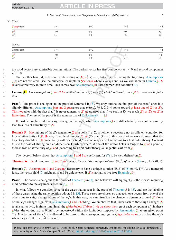
Table 1Q4
Component i = 1 i = 2 i = 3 i = 4
w1i ≤0 >0 <0 <0
w2i >0 ≥0 ≤0 <0
Table 2
Component i = 1 i = 2 i = 3 i = 4
w1i ≤0 >0 ≤0 ≤0
w2i >0 ≥0 ≥0 <0
the solid vectors are admissible configurations. The dashed vector has first component w11 < 0 and second component114
w21 = 0.115
On the other hand, if, as before, while sliding on Σ, w21(x) = 0, but w1
1(x) > 0 along the trajectory, Assumptions116
1(a) are not violated, (see the numerical example in Section 4 where x = x5) and, as we will show in Lemma 4, Σ117
retains attractivity in finite time. This shows how Assumptions 1(a) are sharper than condition (9).118
Lemma 4. Let Assumptions 1 and 2 be verified and let (1±a ) and (2±
a ) hold uniformly, then Σ is attractive in finite119
time.120
Proof. The proof is analogous to the proof of Lemma 4 in [3]. We only outline the first part of the proof since it is121
slightly different. Assumptions 1(a) and 2 guarantee that every fj, j = 1, 2, 3, 4 points toward at least one of Σ1 or Σ2.122
This, together with the fact that fj is never tangent to Σ, guarantees that if we start in Rj, we reach Σ1 or Σ2 or Σ in123
finite time. The rest of the proof is the same as that of [3, Lemma 4]. �124
It must be emphasized that a sign change of the wij’s, while Assumptions 1 are still satisfied, does not necessarily125
lead to a loss of attractivity of Σ.126
Remark 5. Having one of the fj’s tangent to Σ at a point x ∈ Σ, is neither a necessary not a sufficient condition for127
loss of attractivity of Σ. Hence, if, while sliding on Σ, w1j (x) = w2
j (x) = 0, this does not necessarily mean that the128
trajectory should exit Σ tangentially with vector field fj, as one may expect according to a first order theory. Contrast129
this to the case of sliding on a co-dimension 1 surface where, if one of the vector fields is tangent to Σ at a point x,130
there is loss of attractivity of Σ and (according to a first order theory) a tangential exit from Σ.131
The theorem below shows that Assumptions 1 and 2 are sufficient for (7) to be well defined on Σ.132
Theorem 6. Let Assumptions 1 and 2 hold. Then, there exists a unique solution (α, β) of system (8) in (0, 1) × (0, 1).133
Remark 7. Assumptions 1 and 2 are not necessary to have a unique solution (α, β) of (8) on (0, 1)2. As a matter of134
facts, the vector field (7) might exist and be unique even if Σ is not attractive (see Example 10).135
Proof. The proof is analogous to the proof of Theorem 3 in [3], and below we will highlight just those cases requiring136
modifications to the arguments used in [3]. �137
In what follows we consider some of the cases that appear in the proof of Theorem 3 in [3], and use the labeling138
of these cases using the same notation adopted in [3]. These cases are chosen so that each one occurs from one of the139
others due to a sign change of one of the wij’s. In this way, we can visualize the change in dynamics around Σ if one140
of the wij’s changes sign, with Assumptions 1 and 2 holding. We emphasize that under each of these sign changes Σ141
retains attractivity in finite time. In all the tables below (Tables 1–4) we show the sign of each component wij; in these142
tables, the writing ≥0, ≤ 0, must be understood within the limitations imposed by Assumption 2: at any given point143
x ∈ Σ only one of the wij’s is allowed to be zero. In the corresponding figures (Figs. 3–6) we only display the wi
j’s144
when they are all different from zero.145

Please cite this article in press as: L. Dieci, et al. Sharp sufficient attractivity conditions for sliding on a co-dimension 2discontinuity surface, Math. Comput. Simul. (2014), http://dx.doi.org/10.1016/j.matcom.2013.12.005
ARTICLE IN PRESS+ModelMATCOM 4028 1–12
6 L. Dieci et al. / Mathematics and Computers in Simulation xxx (2014) xxx–xxx
Table 3
Component i = 1 i = 2 i = 3 i = 4
w1i ≤0 >0 ≥0 <0
w2i >0 ≥0 >0 <0
Table 4
Component i = 1 i = 2 i = 3 i = 4
w1i ≥0 >0 ≤0 ≤0
w2i ≥0 ≥0 ≥0 <0
Fig. 3. Case SΣ+1
: 2.
Case (SΣ+1
: 2) The signs of the entries of w1 and w2 are as in Table 1, and the following condition is satisfied146
w22
w12
<w2
4
w14
. (10)147
Condition (10) ensures sliding along Σ+1 toward Σ.148
According to Assumptions 1, w11 can be zero on Σ since w2
1 > 0, and similarly for w22 and w2
3.149
Notice, instead, that w14 must be bounded away from zero even though w2
4 < 0. This is in order to150
ensure sliding on at least one of the co-dimension 1 surfaces. Indeed assume that, while following151
Fig. 4. Case SΣ+1 ,Σ+
2: 2.

Please cite this article in press as: L. Dieci, et al. Sharp sufficient attractivity conditions for sliding on a co-dimension 2discontinuity surface, Math. Comput. Simul. (2014), http://dx.doi.org/10.1016/j.matcom.2013.12.005
ARTICLE IN PRESS+ModelMATCOM 4028 1–12
L. Dieci et al. / Mathematics and Computers in Simulation xxx (2014) xxx–xxx 7
Fig. 5. Case SΣ+1 ,Σ+
2: 5.
Fig. 6. Case SΣ±1 ,Σ+
2: 2.
a trajectory on Σ, at t = T, w14(x(T )) = 0. Then for t > T and t sufficiently close to T, w1
4(x(t)) > 0152
and there is no sliding on a co-dimension 1 surface. This is against Assumptions 1(b).153
Case (SΣ+1 ,Σ+
2: 2) This case follows from Case (SΣ+
1: 2) above, here w2
3 has undergone a sign change.154
The signs of the entries of w1 and w2 are as in Table 2 and (10) is satisfied. See Fig. 4.155
Case (SΣ+1 ,Σ+
2: 5) This case follows from Case (SΣ+
1 ,Σ+2
: 2) above, here w13 has undergone a sign change.156
The signs of the entries of w1 and w2 are as in Table 3 and condition (10) is satisfied together157
with the following:158
w13
w23
<w1
4
w24
, (11)159
see Fig. 5.160
Here (1+a ) and (2+
a ) imply that w14 and w2
4 must be different from zero.161
Case (SΣ±1 ,Σ+
2: 2) This case follows from Case SΣ+
1 ,Σ+2
: 2 above after w21 has undergone a sign change.162
The signs of the entries of w1 and w2 are given in Table 4 and (11) is satisfied; see Fig. 6.163
For this configuration (1+a ) implies that w2
4 must be different from zero.164
Example 8. Here we illustrate all the changes in dynamics that might occur while sliding on Σ under Case (SΣ+1 ,Σ+
2:165
2), when one of the components allowed to be zero in Table 2 goes to zero. Suppose that, while following a trajectory166

Please cite this article in press as: L. Dieci, et al. Sharp sufficient attractivity conditions for sliding on a co-dimension 2discontinuity surface, Math. Comput. Simul. (2014), http://dx.doi.org/10.1016/j.matcom.2013.12.005
ARTICLE IN PRESS+ModelMATCOM 4028 1–12
8 L. Dieci et al. / Mathematics and Computers in Simulation xxx (2014) xxx–xxx
Table 5
Component i = 1 i = 2 i = 3 i = 4
w1i −1 1 −1 −0.5
w2i 0 1 −1 −1
Fig. 7. Example 10, wij’s at t = T.
x(t) on Σ, one of the wij’s is zero at time t = T. We will list here all the possible changes in dynamic that occur after167
time T.168
(1) If w11(T ) = 0, then the dynamic after time T is the one in Case (SΣ±
1 ,Σ+2
: 2).169
(2) If w13(T ) = 0, then the dynamic after time T is the one in Case (SΣ+
1 ,Σ+2
: 5).170
(3) If w23(T ) = 0, then the dynamic after time T is the one in Case (SΣ+
1: 2).171
(4) If w14(T ) = 0, then after time T there is attractive sliding only along Σ+
2 and there is no sliding along Σ+1 .172
Trajectories in a neighborhood of Σ will cross Σ+1 in the direction of R4. This case mirrors to Case (SΣ+
1: 2).173
(5) If w22(T ) = 0, then after time T there is attractive sliding toward Σ along Σ+
1 and Σ±2 . This case mirrors Case174
(SΣ±1 ,Σ+
2: 2).175
We stress that Σ is attractive in a neighborhood of x(T), and that (7) is well defined.176
Just like in [3, Theorem 8], and with the same proof, the following holds.177
Theorem 9. Under Assumptions 1 and 2, the unique solution (α, β) ∈ (0, 1) × (0, 1) of system (8) varies smoothly178
with respect to x ∈ Σ.179
3.1. Loss of attractivity180
In [3] we showed that violating any of (1±) or (2±) in Assumptions 1 leads to a loss of attractivity of Σ. We further181
identified when/how this loss of attractivity conduced to an exit from Σ to slide on one of Σ±1,2: first order exit condition.182
Now, when only one of the wij’s is zero, and Assumptions 1 are not satisfied, then Σ looses attractivity, but the183
vector field (7) might still be defined on Σ as showed in Example 10.184
Example 10. Assume that we are following a trajectory on Σ with the wij’s as in Table 1. Moreover, assume that all185
the wij’s are bounded away from zero for t < T and that at time t = T they are as in Table 5 and Fig. 7. As it is clear from186
Fig. 7, at x(T) Assumptions 1 are not satisfied and Σ loses attractivity at time t = T. Nonetheless, system 8 still admits187
a unique solution (α, β) � (0.4226, 0.7321), hence the vector field (7) is still well defined on Σ.188

Please cite this article in press as: L. Dieci, et al. Sharp sufficient attractivity conditions for sliding on a co-dimension 2discontinuity surface, Math. Comput. Simul. (2014), http://dx.doi.org/10.1016/j.matcom.2013.12.005
ARTICLE IN PRESS+ModelMATCOM 4028 1–12
L. Dieci et al. / Mathematics and Computers in Simulation xxx (2014) xxx–xxx 9
In Remark 5, we noticed how, while sliding on Σ, fj might be tangent to Σ without this implying a loss of attractivity189
of Σ. Here, in Remark 11, we emphasize how a co-dimension 2 sliding surface might lose attractivity at a point x even190
though there is no potential tangential exit vector field at that point.191
Remark 11. Consider again Table 5. Note that Σ has lost attractivity, but there is no tangential vector field exiting Σ.192
This is in distinct contrast with sliding on a co-dimension 1 surface. In the latter case, indeed, when the sliding surface193
Σ looses attractivity, Filippov theory will predict (at first order) exiting Σ tangentially.194
4. Numerical example195
Here we result of numerical experiments on an example where one of the wij’s (namely, w1
2) becomes 0 along the196
sliding trajectory, still satisfying Assumptions 1. Aside from the modification due to w12 becoming 0, the example197
below is actually the one we meant to use in [3].198
All computations have been made with an event driven technique, and event points (when a different regime is199
reached) have been computed by the secant method. Integration of all relevant differential equations was made using200
the classical explicit Runge–Kutta (RK) scheme of order four, a projected RK method in case of sliding motion to201
ensure that all evaluations are made on the constraints’ surfaces (e.g., see [4]). The stepsize τ was held constant and202
equal to τ = 0.0025, and of course adjusted when using the secant method to locate event points. Solution of the system203
(8) was done by Newton’s method.204
Example 12. We have the discontinuity surfaces205
Σ1 = {x ∈ R3 : h1(x) = x2 − p}, Σ2 = {x ∈ R3 : h2(x) = x3 − q}, Σ = Σ1 ∩ Σ2206
with p = 0.5 and q = 1. Thus, we have the following four vector fields, at least continuous in their respective regions of207
definition:208
R1(h1 < 0, h2 < 0) : f1(x) =
⎛⎜⎜⎜⎜⎜⎝
x2
−x1 + 1
(1 + p) − x2
−x1 + 32
−1
(1 + q) − x3
⎞⎟⎟⎟⎟⎟⎠ ;209
R2(h1 < 0, h2 > 0) : f2(x) =
⎛⎜⎜⎜⎜⎜⎝
−(x2 + x3)
−x1 + 1
(1 + p) − x2
−x1 − 1
(1 − q) + x3
⎞⎟⎟⎟⎟⎟⎠ ;210
R3(h1 > 0, h2 < 0) : f3(x) =
⎧⎪⎪⎪⎪⎪⎪⎪⎪⎪⎪⎪⎪⎪⎪⎪⎪⎪⎪⎪⎨⎪⎪⎪⎪⎪⎪⎪⎪⎪⎪⎪⎪⎪⎪⎪⎪⎪⎪⎪⎩
⎛⎜⎜⎜⎜⎜⎜⎝
−(x2 + x3)
−x1 + 1
(1 − p) + x2
−x1 + 1
(1 + q) − x3
⎞⎟⎟⎟⎟⎟⎟⎠
when x1≥ − 1.3,
⎛⎜⎜⎜⎜⎜⎜⎝
−(x2 + x3)
6 + 1.3 + 6x1
1.3+ 1
(1 − p) + x2
−x1 + 1
(1 + q) − x3
⎞⎟⎟⎟⎟⎟⎟⎠
when x1 < −1.3,
211

Please cite this article in press as: L. Dieci, et al. Sharp sufficient attractivity conditions for sliding on a co-dimension 2discontinuity surface, Math. Comput. Simul. (2014), http://dx.doi.org/10.1016/j.matcom.2013.12.005
ARTICLE IN PRESS+ModelMATCOM 4028 1–12
10 L. Dieci et al. / Mathematics and Computers in Simulation xxx (2014) xxx–xxx
−0.5
0
0.5
1
0.5
0.51
0.52
0.53
0.98
0.99
1
1.01
1.02
1.03
x2x1
x3
Σ
x0
x1
x2
x3
x4
x5
x6
Fig. 8. Solution trajectory: the solution spirals around Σ, starts sliding on Σ+1 , enters Σ and leaves it to slide on Σ+
1 .
−3
−2
−1
0
1
0.40.5
0.60.7
0.80.9
1
1
1.1
1.2
1.3
1.4
1.5
1.6
1.7
1.8
x2x1
x3 R4
Σ1+
Σ2+
x6
x7
x8
x11
x9
x10
Fig. 9. Solution trajectory: the solution slides on Σ+1 and leaves it to enter R4, hits Σ+
2 and starts sliding on it, then hits Σ and starts sliding on it.
R4(h1 > 0, h2 > 0) : f4(x) =
⎧⎪⎪⎪⎪⎪⎪⎪⎪⎪⎪⎪⎪⎪⎪⎪⎪⎪⎪⎨⎪⎪⎪⎪⎪⎪⎪⎪⎪⎪⎪⎪⎪⎪⎪⎪⎪⎪⎩
⎛⎜⎜⎜⎜⎜⎜⎝
−(x2 + x3)
−x1 − 1
(1 − p) + x2
−x1 + 1
(1 − q) + x3
⎞⎟⎟⎟⎟⎟⎟⎠
when x1≥ − 1,
⎛⎜⎜⎜⎜⎜⎜⎝
−(x2 + x3)
−x1 − 1
(1 − p) + x2
130 + 129x1 + 1
(1 − q) + x3
⎞⎟⎟⎟⎟⎟⎟⎠
when x1 < −1.
212
Results below are for initial condition x0 = [0.7, 0.49, 0.99]. We can distinguish several different dynamics of the213
solution with respect to the two discontinuity surfaces. Indeed, there are several event points, that is values where the214
solution reaches a different regime: a different region and/or sliding surface. We will assign a time value tj, and with215
abuse of notation indicate each event point with xj. The initial part of the trajectory is plotted in Fig. 8, and Fig. 9 shows216
the entire trajectory; event points are marked by asterisks: xj, j = 1, . . ., 11.217

Please cite this article in press as: L. Dieci, et al. Sharp sufficient attractivity conditions for sliding on a co-dimension 2discontinuity surface, Math. Comput. Simul. (2014), http://dx.doi.org/10.1016/j.matcom.2013.12.005
ARTICLE IN PRESS+ModelMATCOM 4028 1–12
L. Dieci et al. / Mathematics and Computers in Simulation xxx (2014) xxx–xxx 11
Table 6wi
j’s at x4.
Component i = 1 i = 2 i = 3 i = 4
w1i >0 >0 >0 <0
w2i <0 <0 >0 >0
Fig. 10. w1 = (w11, w
21) at t < t5 (left), at t5 (center), and at t > t5 (right).
The initial condition is in region R1 and the trajectory crosses Σ−1 at x1 ≈ (0.71728, 0.5, 0.98318) and enters R3218
(transversal intersection). At x2 ≈ (0.63696, 0.51686, 1), it crosses Σ+2 and enters R4 (transversal intersection). At219
x3 ≈ (0.62125, 0.5, 1.00384), it hits Σ+1 and starts sliding on it in the direction of Σ with vector field fΣ+
1. Then, while220
sliding on Σ+1 the solution reaches Σ at time t4 at the point x4 ≈ (0.61659, 0.5, 1).221
At x4, the vector fields fj, j = 1, 2, 3, 4, have the signs given in Table 6 and condition (10) is satisfied, so that222
Assumptions 1 are satisfied, Σ is attractive, fΣ as in (7) is well defined and the solution starts sliding on Σ.223
At time t5, the solution is at x5 = (0.5, 0.5, 1), w21(x5) = 0, and w1
1 /= 0 for values on Σ in a neighborhood of x5.224
Assumptions 1 and 2 are satisfied at x5, so the solution keeps sliding on Σ. The configuration along the solution path225
in a neighborhood of t5 is the one showed in Fig. 10 (it mirrors Case (SΣ+1 ,Σ+
2: 1) in [3]). Here the dashed vector is226
w1 = (w11, w
21) at a specific time t < t5, the dotted vector is w1(x(t5)) and the solid vector is w1 at a specific time t > t5.227
At t = t6 ≈ 0.62925, the solution is at x6 = (0, 0.5, 1), and there is equality in (10). Moreover, the wij(x)’s for x = x6228
are as in Table 7 and the trajectory leaves Σ smoothly to enter Σ+1 .229
So, at t = t6, fΣ aligns to fΣ+1
and the solution exits Σ smoothly to slide on Σ+1 . At time t7 ≈ 1.22698, the solution230
reaches x7 ≈ (−1, 0.5, 1.5111), fΣ+1
aligns to f4 and the solution exits Σ+1 smoothly to enter in region R4. At time t8,231
it reaches Σ+2 at x8 ≈ (−1.1322, 0.5050, 1), and here w2
3 > 0 while w24 < 0 so that sliding begins on Σ+
2 away from232
Σ1. At time t9 ≈ 1.40259, the solution reaches the surface x1 = −1.3 at x9 ≈ (−1.3, 0.7105, 1); here, f3 is continuous233
Table 7wi
j’s at x6.
Component i = 1 i = 2 i = 3 i = 4
w1i 1 1 1 −1
w2i
12 −1 1 1

Please cite this article in press as: L. Dieci, et al. Sharp sufficient attractivity conditions for sliding on a co-dimension 2discontinuity surface, Math. Comput. Simul. (2014), http://dx.doi.org/10.1016/j.matcom.2013.12.005
ARTICLE IN PRESS+ModelMATCOM 4028 1–12
12 L. Dieci et al. / Mathematics and Computers in Simulation xxx (2014) xxx–xxx
Table 8wi
j’s at x11.
Component i = 1 i = 2 i = 3 i = 4
w1i >0 >0 <0 >0
w2i >0 >0 >0 <0
but not differentiable. At time t10, we reach the value x10 ≈ (−1.7377, 0.9507, 1). For t > t10 the trajectory continues234
sliding on Σ+2 but now in the direction of Σ1, since the following condition is satisfied:235
w13
w23
<w1
4
w24
. (12)236
At time t11, the solution reaches the point x11 ≈ (−2.3430, 0.5, 1) on Σ. The vector fields fj(x10), j = 1, . . ., 4, satisfy237
the conditions of Table 8 and the behavior on Σ is analogous to the one of Case (SΣ+1
: 2). The solution now starts238
sliding on Σ with vector field fΣ as in (7), and remains on Σ.239
5. Conclusions240
In this paper we weakened the assumptions given in [3] for attractivity of a sliding co-dimension 2 surface Σ and241
for the existence and uniqueness of the Filippov sliding vector field (7) on Σ. We reported on a numerical experiment242
to show the behavior of a piecewise smooth system that satisfies our new assumptions.243
References244
[1] V. Acary, B. Brogliato, Numerical Methods for Nonsmooth Dynamical Systems. Applications in Mechanics and Electonics, Lecture Notes in245
Applied and Computational Mechanics, Springer-Verlag, Berlin, 2008.246
[2] J. Alexander, T. Seidman, Sliding modes in intersecting switching surfaces. I: Blending, Houston J. Math. 24 (1998) 545–569.247
[3] L. Dieci, C. Elia, L. Lopez, A Filippov sliding vector field on an attracting co-dimension 2 discontinuity surface, and a limited loss-of-attractivity248
analysis, J. Differ. Equat. 254 (2013) 1800–1832.249
[4] L. Dieci, L. Lopez, Sliding motion in Filippov differential systems: theoretical results and a computational approach, SIAM J. Numer. Anal. 47250
(2009) 2023–2051.251
[5] L. Dieci, L. Lopez, Sliding motion on discontinuity surfaces of high codimension. A construction for selecting a Filippov vector field, Numer.252
Math. 117 (2011) 779–811.253
[6] A. Filippov, Differential Equations with Discontinuous Right-Hand Sides, Mathematics and its Applications, Kluwer Academic, Dordrecht,254
1988.255