RESEARCH ARTICLE

Diagnosing the Dynamics of Observed and

Simulated Ecosystem Gross Primary

Productivity with Time Causal Information

Theory Quantifiers

Sebastian Sippel1*, Holger Lange2,3, Miguel D. Mahecha1,4,5, Michael Hauhs6,

Paul Bodesheim1, Thomas Kaminski7, Fabian Gans1, Osvaldo A. Rosso3,8,9

1 Max Planck Institute for Biogeochemistry, Jena, Germany, 2 Norwegian Institute of Bioeconomy Research,

Ås, Norway, 3 Instituto de Fısica, Universidade Federal de Alagoas, Maceio, Alagoas, Brazil, 4 German

Centre for Integrative Biodiversity Research (iDiv), Leipzig, Germany, 5 Michael Stifel Center Jena for Data-

Driven and Simulation Science, Jena, Germany, 6 University of Bayreuth, Bayreuth, Germany, 7 The

Inversion Lab, Hamburg, Germany, 8 Instituto Tecnologico de Buenos Aires (ITBA) and CONICET, Ciudad

Autonoma de Buenos Aires, Argentina, 9 Complex Systems Group, Facultad de Ingenierıa y Ciencias

Aplicadas, Universidad de los Andes, Las Condes, Santiago, Chile

* ssippel@bgc-jena.mpg.de

Abstract

Data analysis and model-data comparisons in the environmental sciences require diagnos-

tic measures that quantify time series dynamics and structure, and are robust to noise in

observational data. This paper investigates the temporal dynamics of environmental time

series using measures quantifying their information content and complexity. The measures

are used to classify natural processes on one hand, and to compare models with observa-

tions on the other. The present analysis focuses on the global carbon cycle as an area of

research in which model-data integration and comparisons are key to improving our under-

standing of natural phenomena. We investigate the dynamics of observed and simulated

time series of Gross Primary Productivity (GPP), a key variable in terrestrial ecosystems

that quantifies ecosystem carbon uptake. However, the dynamics, patterns and magni-

tudes of GPP time series, both observed and simulated, vary substantially on different tem-

poral and spatial scales. We demonstrate here that information content and complexity, or

Information Theory Quantifiers (ITQ) for short, serve as robust and efficient data-analytical

and model benchmarking tools for evaluating the temporal structure and dynamical proper-

ties of simulated or observed time series at various spatial scales. At continental scale, we

compare GPP time series simulated with two models and an observations-based product.

This analysis reveals qualitative differences between model evaluation based on ITQ com-

pared to traditional model performance metrics, indicating that good model performance in

terms of absolute or relative error does not imply that the dynamics of the observations is

captured well. Furthermore, we show, using an ensemble of site-scale measurements

obtained from the FLUXNET archive in the Mediterranean, that model-data or model-model

mismatches as indicated by ITQ can be attributed to and interpreted as differences in the

temporal structure of the respective ecological time series. At global scale, our

PLOS ONE | DOI:10.1371/journal.pone.0164960 October 20, 2016 1 / 29

a11111

OPENACCESS

Citation: Sippel S, Lange H, Mahecha MD, Hauhs

M, Bodesheim P, Kaminski T, et al. (2016)

Diagnosing the Dynamics of Observed and

Simulated Ecosystem Gross Primary Productivity

with Time Causal Information Theory Quantifiers.

PLoS ONE 11(10): e0164960. doi:10.1371/journal.

pone.0164960

Editor: Ben Bond-Lamberty, Pacific Northwest

National Laboratory, UNITED STATES

Received: April 28, 2016

Accepted: October 4, 2016

Published: October 20, 2016

Copyright: © 2016 Sippel et al. This is an open

access article distributed under the terms of the

Creative Commons Attribution License, which

permits unrestricted use, distribution, and

reproduction in any medium, provided the original

author and source are credited.

Data Availability Statement: We have gathered

the data from various data providers specifically to

conduct the complexity analysis as presented in

this paper. Therefore, the original data are indeed

third party data, hence it is not our property and we

cannot make it public. However, we give very

specific information below, and all data is available

from the data providers as indicated below: 1. The

JRC-TIP FAPAR dataset is made available by the

European Commission and the Inversion Lab, as

indicated in the manuscript. The JRC-TIP FAPAR

understanding of C fluxes relies on the use of consistently applied land models. Here, we

use ITQ to evaluate model structure: The measures are largely insensitive to climatic sce-

narios, land use and atmospheric gas concentrations used to drive them, but clearly sepa-

rate the structure of 13 different land models taken from the CMIP5 archive and an

observations-based product. In conclusion, diagnostic measures of this kind provide data-

analytical tools that distinguish different types of natural processes based solely on their

dynamics, and are thus highly suitable for environmental science applications such as

model structural diagnostics.

Introduction

Understanding the feedback between terrestrial ecosystems and changing environmental con-ditions is a key prerequisite to model the impact of global change. Of particular relevance arechanges in the global carbon (C from now on) cycle, i.e. in land-atmosphere fluxes and thusbiosphere carbon stocks (e.g. [1]). Today, empirical and process-based models of varying struc-tural and numerical complexity are used to assess and predict past, present and future ecosys-tem-atmosphere carbon exchange (e.g. [2]).

The state of current process-based understanding is in part implemented in terrestrial bio-sphere models. The process representations in these models differ widely, which is in part dueto insufficient mechanistic understanding of the underlying processes or uncertain parameterestimates. This lack of consensus leads to major uncertainties in the predictions [3]. The start-ing point to reduce uncertainties in modelled fluxes or physiological state variables is to quan-tify their mismatch with observations [4].

Model benchmarking seeks to quantify this mismatch and to rank the models accordingly[5–9]. Obviously, model rankings depend on the metric(s) considered; it is unlikely that onesingle model will rank best with respect to multiple metrics that may emphasize differentaspects.

Activities such as the International Land Model Benchmarking Project (ILAMB, http://ilamb.org) have formalized this idea by providing a range of benchmarks. In order to standard-ize the benchmarking approaches further, several platforms for automatic benchmarking havebeen developed [2, 7]. Most of the metrics used for benchmarking so far are straightforward,for instance focusing on long-term mean values per variable and pixel (or region), or the ampli-tude of some specific seasonal cycle (e.g. of some land-atmosphere flux). However, metrics ofthis kind can only provide a limited insight into the dynamics of the models under scrutiny.Consequently, latest benchmarking efforts intend to consider relevant observed and simulatedpatterns, such as process efficiencies or turnover-rates [10], i.e. these approaches attempt toderive a pattern-oriented strategy to model evaluation and model-data integration [11–13].Hence, various initiatives to land surface model benchmarking are still working towards devel-oping a widely acceptable set of benchmarks [8] that target various relevant aspects of modelbehaviour.

One difficulty in model benchmarking is that reference data are potentially affected byobservational noise or biases. Ideally, models should exhibit similar dynamics as the observa-tions on a range of time scales [14]. Disagreements of models and observations indicate eitherinaccurate parameter estimates, structural deficits, or other inadequacies of the models; or theyoriginate in low quality of the reference observations, with e.g. noise contamination at high fre-quencies and sensor ageing processes at long time scales. Hence, in any model-data comparison

GPP Dynamics and Information Quantifiers

PLOS ONE | DOI:10.1371/journal.pone.0164960 October 20, 2016 2 / 29

dataset was introduced in the following publication:

Pinty B., Clerici M., Andredakis I., Kaminski T.,

Taberner M., Verstraete M. M., Gobron N.,

Plummer S. and Widlowski J.-L. (2011) Exploiting

the MODIS Albedos with the Two-stream Inversion

Package (JRC-TIP) Part II: Fractions of transmitted

and absorbed fluxes in the Vegetation and Soil

layers, Journal of Geophysical Research-

Atmospheres, 116, D09106, doi:10.1029/

2010JD015373. 2. For the site-based time series of

GPP dataset, we use the well-known La-Thuile

Synthesis Dataset (as described in the

manuscript), available from http://fluxnet.fluxdata.

org/data/la-thuile-dataset/. It’s available based on a

fair-use policy, hence everyone can request, use

and download the dataset from the given URL. 3.

The specific URL to access the GPP model runs

data is https://www.bgc-jena.mpg.de/geodb/

projects/Data.php. Everyone can download the data

after a data usage agreement has been made with

the owners of the data. 4. The specific URL to

access CMIP5 data is https://pcmdi.llnl.gov/search/

cmip5/, and the related publication is: Taylor, K.E.,

Stouffer, R.J. and Meehl, G.A., 2012. An overview

of CMIP5 and the experiment design. Bulletin of the

American Meteorological Society, 93(4), p.485.

DOI: http://dx.doi.org/10.1175/BAMS-D-11-00094.

1.

Funding: This work was supported by German

National Academic Foundation, http://www.

studienstiftung.de (no grant number), SS

(Studienstiftung des Deutschen Volkes); Consejo

Nacional de Investigaciones Cientıficas y Tecnicas

(CONICET), Argentina, http://www.conicet.gov.ar

(no grant number), OAR; Conselho Nacional de

Desenvolvimento Cientıfico e Tecnologico (CNPq),

http://cnpq.br, Grant number 310003/2016-4, HL;

European Space Agency, STSE project CAB-LAB

("Coupled Atmosphere Biosphere virtual

LABoratory"), http://earthsystemdatacube.net,

MDM FG PB SS; European Commission, BACI

project ("Detecting changes in essential ecosystem

and biodiversity properties - towards a Biosphere

Atmosphere Change Index"), http://baci-h2020.eu/

index.php/ (Grant number 640176), MDM SS.

Competing Interests: The authors have declared

that no competing interests exist.

such as benchmarking, a distinction between signal and noise is necessary. In the interpretationof data analysis, signal extraction from the noise background is key; process-oriented modelsshould be able to reproduce the signal but not the noise part of observations.

Here, we contribute to the discussion of model evaluation and benchmarking by investigat-ing the potential of Information Theory Quantifiers (ITQ) as an additional set of benchmarkingtools, with a special focus on the dynamics and structure of model simulated vs. observed timeseries. For example, questions such as ‘How much information do the observations reveal aboutthe dynamics of the underlying system or processes? Do observed time series resemble stochasticor deterministic processes? Are models reproducing the observed process classes?’ arise naturallyfrom an Information Theory perspective and could potentially be tackled using ITQ. Thesemeasures draw a distinction between deterministic and stochastic processes, are complemen-tary to the present set of tools and might thus provide a balanced investigation of model evalua-tion, e.g. sensu [6].

Among the set of variables established to describe C dynamics, the gross CO2 uptake of ter-restrial vegetation from the atmosphere (‘Gross Primary Productivity’, or GPP) is of particularimportance for terrestrial ecosystems. GPP can be derived from in-situ measurements of netecosystem exchange fluxes of CO2. GPP is predominantly controlled by radiation, but likewisesensitive to temperature, CO2 concentrations, water availability and the phenological status ofthe vegetation, amongst other factors [15]. GPP is routinely obtained as the difference of NetEcosystem Productivity (NEP) measurements and estimates for ecosystem respiration (Reco) atindividual sites as part of a global monitoring network [16]. GPP is expected to show seasonalvariation; abrupt changes or systematic trends in GPP can be induced by land use change,extreme events, and changing climate, among other factors. Numerous attempts to quantifyGPP at larger spatial scales exist, but many of these rely on dynamical global vegetation andbiogeochemical models. Based on assumed biological and physical processes, the latter eithertry to reconstruct historical GPP time series, based on observed precipitation, radiation, tem-perature and other drivers, or project the future dynamics of GPP using climate scenarios (Rep-resentative Concentration Pathways, RCPs [17]). Generally, GPP simulations respond globallyto transient climate change, but locally and regionally also to abrupt land use changes, orextreme hydrometeorological anomalies [18, 19].

This study aims to introduce and interpret ITQ in the context of environmental time seriesanalysis with particular emphasis on model evaluation and benchmarking of GPP dynamics atsite, continental and global scale. The paper is organized as follows: the Section Quantifiersfrom Information Theory” provides an introduction to the field of ordinal pattern statisticsand the associated Information Theory Quantifiers. “Data Sets Investigated” introduces thedata: observations and model simulations of GPP at the site, continental and global scale; and aremotely sensed widely used proxy for vegetation activity (‘Fraction of Absorbed Photosynthet-ically Active Radiation’ (FAPAR)). The subsection “An Information Theory perspective onspatio-temporal environmental datasets” provides an intuitive introduction to ITQ in the con-text of environmental science using i) a FAPAR dataset at continental-scale and high spatialresolution; and ii) in-situ GPP measurements from flux tower sites to illustrate the effects oftemporal resolution from the FLUXNET database, cf. http://fluxnet.fluxdata.org [16]. Then, weproceed by comparing the complexity and information content of GPP time series simulatedby two process-based ecosystem models and an observations-based dataset at continental scalein a spatially explicit manner; these results are augmented with site-scale flux tower measure-ments. In “Global analysis of land surface models”, ITQ calculated from global-scale modelsimulations of GPP obtained from a climate model intercomparison project (CMIP5) compris-ing both historical reconstructions and climate scenario runs (1861-2090; ‘scenarios’) are eval-uated to diagnose model structure. Finally, we conclude on the suitability of Information

GPP Dynamics and Information Quantifiers

PLOS ONE | DOI:10.1371/journal.pone.0164960 October 20, 2016 3 / 29

Theory Quantifiers for environmental science applications, such as diagnosing model structureor model benchmarking.

Quantifiers from Information Theory

Given a time series or other observational data, a natural question arises: how much informa-tion are these data revealing about the dynamics of the underlying system or processes? Theinformation content of data sets is typically evaluated via characterizing a value distribution ora probability density function (PDF) P describing the apportionment of some measurable orobservable quantity [20]. These quantifiers represent metrics on the space of PDFs for datasets, allowing to compare different sets and to classify them according to the properties ofunderlying processes—broadly, stochastic vs. deterministic. Here, we refer to stochastic pro-cesses like correlated noise on one hand, and to deterministic chaotic maps which do not con-tain any noise on the other. Time series generated by these two categories of processes aredifficult to discern by conventional analysis, but are clearly separated by ITQ [21].

In our case, we are interested in the temporal dynamics of GPP, and our data are time seriesx(t). Thus, we are mostly interested in metrics which take the temporal order of observationsexplicitly into account; i.e. the approach is fundamentally a causal rather than a statistical one.In a purely statistical approach, correlations between sucessive values from the time series areignored or simply destroyed via construction of the PDF; while a causal approach focuses onthe PDFs of data sequences.

The quantifiers selected are based on ordinal pattern statistics (cf. e.g. [22]). For an applicationof alternative quantifiers based on Symbolic Dynamics to environmental data, we refer to [23].The quantifiers used here belong to either of two broad categories: those which quantify the infor-mation content of data versus those related to their complexity on one hand; and metrics relatedto global properties of the appropriate PDFs versus ones which take local properties into account.Note that we are referring to the space of probability density functions here, not physical space.For the sake of clarity and simplicity, we introduce Information Theory quantifiers that aredefined on discrete PDFs in this section, since we are only dealing with discrete data (time series).However, all the quantifiers also have definitions for the continuous case [24, 25].

The Shannon entropy as a measure for information content

The permutation Shannon entropy is a measure for the information content of the time series[24] and quantifies uncertainty, disorder, state-space volume, and lack of information [26]. LetP = {pi; i = 1, . . ., N} with

PNi¼1pi ¼ 1, be a probability distribution, withN possible states of

the system under study. The Shannon information measure (entropy) reads

S½P� ¼ �XN

i¼1

pi ln ½pi� : ð1Þ

The Shannon entropy is minimal when all but one of the pi’s vanish, and maximal when allpi’s are equal, i.e. for the uniform distribution Pe ¼ fpi ¼ 1

N ; 8i ¼ 1; . . . ;Ng. In this case,S½Pe� ¼ S max ¼ lnN. However, these two situations are extreme cases, unlikely to occur inany natural phenomenon considered here. In the following, we focus on the ‘normalized’ Shan-non entropy, 0 � H � 1, given as

H½P� ¼ S½P�=S max : ð2Þ

GPP Dynamics and Information Quantifiers

PLOS ONE | DOI:10.1371/journal.pone.0164960 October 20, 2016 4 / 29

Statistical complexity measures

Contrary to information content, there is no universally accepted definition of complexity.Here, we focus on describing the complexity of time series and do not refer to the complexity ofthe underlying systems. In fact, “simple” models might generate complex data, while “compli-cated” systems might produce output data of low complexity [27].

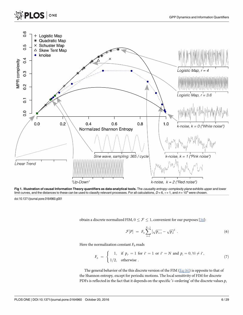
An intuitive notion of a quantitative complexity attributes low values both to perfectlyordered data (i.e. with vanishing Shannon entropy) as well as to uncorrelated random data(with maximal Shannon entropy), as both cases can be well described in a compact manner.For example, the statistical complexity of a simple oscillation or trend (ordered), but also ofuncorrelated white noise (disordered) would be classified as low. Hence, linear transient trendsand measurement noise of some geophysical variable would exhibit small complexity values,but the two processes would differ considerably in their Shannon entropy (Fig 1). Between thetwo cases of minimal and maximal entropy, data are more difficult to characterize and hencethe complexity should be higher. We seek some functional C½P� quantifying structures presentin the data which deviate from these two cases. These structures relate to organization, correla-tional structure, memory, regularity, symmetry, patterns, and other properties [28].

One suitable way to guarantee the desired properties for a complexity measure is to buildthe product of a measure of information and a measure of disequilibrium, i.e. some kind of dis-tance from the uniform (‘equilibrium’) distribution of the accessible states of a system. In thisrespect, in [29] an effective Statistical Complexity Measure (SCM) C was introduced, that isable to detect and discern basic dynamical properties of datasets.

Based on the seminal notion advanced by Lopez-Ruiz et al. [30], this statistical complexitymeasure [29, 31] is defined through the functional product form

C½P� ¼ QJ ½P; Pe� �H½P� ð3Þ

of the normalized Shannon entropy H, see Eq (2), and the disequilibrium QJ ½P; Pe� defined interms of the Jensen-Shannon divergence J ½P; Pe�. The latter is given by

QJ ½P; Pe� ¼ Q0J ½P; Pe� ¼ Q0fS½ðP þ PeÞ=2� � S½P�=2 � S½Pe�=2g; ð4Þ

whereQ0 is a normalization constant chosen such that 0 � QJ � 1:

Q0 ¼ � 2N þ 1

Nln ðN þ 1Þ � ln ð2NÞ þ lnN

� �� 1

: ð5Þ

The inverse of this value is obtained for the non-normalized Jensen-Shannon divergence whenone of the components of P, say pm, is equal to one and the remaining pj’s are zero.

The Jensen-Shannon divergence quantifies the difference between probability distributionsand is especially useful to compare the symbolic composition of different sequences [32]. Notethat the above introduced Information Theory quantifier depends on two different probabilitydistributions: one associated with the system under analysis, P, and the other the uniform dis-tribution Pe. For the latter, other reference distributions can be chosen to test whether anobserved distribution is close to a target distribution. It has been shown that there are limitcurves for complexity: for a given value of H and any data set, the possible C values varybetween a minimum CminðHÞ and a maximum CmaxðHÞ, restricting the possible values of thecomplexity measure [33].

An alternative measure which is local in distribution space is the Fisher Information Mea-sure (FIM). For calculating FIM, we use probability amplitudes as a starting point [25] and

GPP Dynamics and Information Quantifiers

PLOS ONE | DOI:10.1371/journal.pone.0164960 October 20, 2016 5 / 29

obtain a discrete normalized FIM, 0 � F � 1, convenient for our purposes [34]:

F ½P� ¼ F0

XN� 1

i¼1

½ffiffiffiffiffiffiffipiþ1

p�

ffiffiffiffipip�2: ð6Þ

Here the normalization constant F0 reads

F0 ¼1; if pi� ¼ 1 for i� ¼ 1 or i� ¼ N and pi ¼ 0;8i 6¼ i�;

1=2; otherwise :ð7Þ

(

The general behavior of the this discrete version of the FIM (Eq (6)) is opposite to that ofthe Shannon entropy, except for periodic motions. The local sensitivity of FIM for discretePDFs is reflected in the fact that it depends on the specific ‘i–ordering’ of the discrete values pi

Fig 1. Illustration of causal Information Theory quantifiers as data-analytical tools. The causality entropy–complexity plane exhibits upper and lower

limit curves, and the distances to these can be used to classify relevant processes. For all calculations, D = 6, τ = 1, and n = 104 were chosen.

doi:10.1371/journal.pone.0164960.g001

GPP Dynamics and Information Quantifiers

PLOS ONE | DOI:10.1371/journal.pone.0164960 October 20, 2016 6 / 29

[34, 35]. The summands in Eq (6) can be regarded as a ‘distance’ between two contiguous prob-abilities. Thus, a different ordering of the patterns would lead to a different FIM-value, demon-strating its local nature. In the present work, we follow the so-called Keller sorting scheme [36]for the generation of the Bandt and Pompe PDF discussed in the next section.

The Bandt and Pompe approach to generate a causal PDF

The quantifiers from Information Theory rely on a probability distribution associated to thetime series. The determination of the most adequate PDF is a fundamental problem becausethe PDF P and its sample space O are inextricably linked. The usual histogram technique isinadequate since the data are treated purely stochastic and the temporal information iscompletely lost. Bandt and Pompe (BP) [22] introduced a simple and robust symbolic method-ology that takes into account time ordering of the time series by comparing neighboring valuesin a time series. The symbolic data are created by first ranking the values of the series withinwindows of a fixed length, and then reordering these embedded data in ascending order. Thisis tantamount to a phase space reconstruction with embedding dimension (pattern length)Dand time lag τ (see Text 1 in S1 File for a more detailed description). In this way, it is possibleto quantify the diversity of the ordering symbols (patterns) derived from a scalar time series.Note that the appropriate symbol sequence arises naturally from the time series, and nomodel-based assumptions are needed. As such, it allows to uncover important details concern-ing the ordinal structure of the time series [21] and can also yield information about temporalcorrelation [37].

This type of analysis of a time series entails losing details of the original series’ amplitudeinformation. However, the symbolic representation of time series by recourse to a comparisonof consecutive (τ = 1) or nonconsecutive (τ> 1) values allows for an accurate empirical recon-struction of the underlying phase-space, even in the presence of weak (observational anddynamic) noise [22]. Furthermore, the ordinal patterns associated with the PDF are invariantwith respect to nonlinear monotonous transformations; nonlinear drifts or scaling artificiallyintroduced by a measurement device will not modify the estimation of quantifiers, a nice prop-erty if one deals with experimental data (see, e.g., [38]). The only condition for the applicabilityof the BP method is a very weak stationarity assumption: for k� D, the probability for xt< xt+k should not depend on t. For a review of the BP methodology and its applications to physics,biomedical and econophysics signals, see [39].

Regarding the selection of the parameters, Bandt and Pompe suggested working with 4�D� 6 for typical time series lengths, and specifically considered a time lag τ = 1 in their corner-stone paper [22]. For the artificially generated time series shown below (Figs 1 and 2), we choseD = 6 and follow the Lehmer-permutation scheme [35] to calculate the Fisher Information. Forthe measured and modelled time series analyzed here, the embedding dimension is chosen asD = 4 throughout due to time series length requirements (S1 File), in particular at coarse tem-poral resolution, and to achieve comparability across the different analyses. In all cases, thedelay parameter has been set to τ = 1.

Incorporating amplitude information: Weighted ordinal pattern

distribution

Recently, the permutation entropy was extended to incorporate also amplitude information[40]. Hence, a potential disadvantage of ordinal pattern statistics, namely the loss of amplitudeinformation, can be addressed by introducing weights in order to obtain a ‘weighted permuta-tion entropy (WPE)’. In the context of environmental time series, which typically exhibit a pro-nounced seasonal cycle and thus seasonally varying signal to noise ratios, this idea might be

GPP Dynamics and Information Quantifiers

PLOS ONE | DOI:10.1371/journal.pone.0164960 October 20, 2016 7 / 29

particularly useful to address (noisy) low-variance patterns (e.g. during dormancy periods inwinter).

Weighting the probabilities of individual patterns according to their variance alleviatespotential issues regarding to ‘high noise, low signal’ patterns, because low-variance patternsthat are stronlgy affected by noise are down-weighted in the resulting ‘weighted ordinal patterndistributions’. For example, [40] show that a weighted entropy measure is sensitive to suddenchanges in the variance of the time series. Here, we extend the idea of WPE following [40] toderive a weighted permutation entropy (Hw), weighted statistical complexity (Cw), andweighted Fisher Information (Fw).

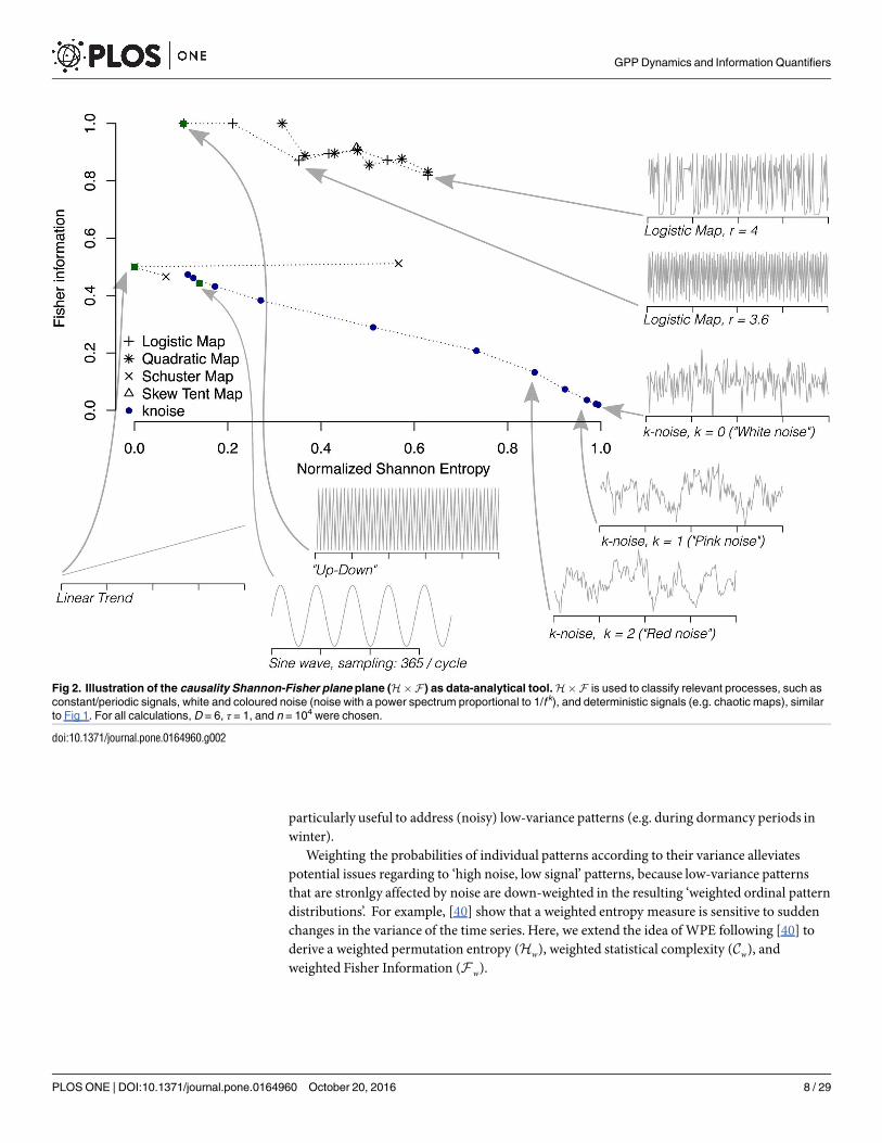
Fig 2. Illustration of the causality Shannon-Fisher plane plane (H� F ) as data-analytical tool. H� F is used to classify relevant processes, such as

constant/periodic signals, white and coloured noise (noise with a power spectrum proportional to 1/f k), and deterministic signals (e.g. chaotic maps), similar

to Fig 1. For all calculations, D = 6, τ = 1, and n = 104 were chosen.

doi:10.1371/journal.pone.0164960.g002

GPP Dynamics and Information Quantifiers

PLOS ONE | DOI:10.1371/journal.pone.0164960 October 20, 2016 8 / 29

Non-normalized weights are computed for each temporal window for the time seriesX,such that

wj ¼1

D

XD

k¼1

ðxjþk� 1 � XDj Þ

2: ð8Þ

Here, the embedding dimension is denoted by D and XDj denotes the arithmetic mean of the

time series in the current window with index j. Thus, the weight of each window of length D isgiven by its variance in the equation above. The weights wj are then used to modify the relativefrequencies of each ordinal pattern pjðXD

j Þ, with N − D + 1 windows, given byXDj ¼ ðxj; xjþ1; :::; xjþD� 1Þ, for a time series of lengthN [40]:

pwðpiÞ ¼

PN� Dþ1

j¼1dpi ;pj

wjPN� Dþ1

k¼1wk

ð9Þ

The denominator of this equation provides the normalization, and the Kronecker delta δπi πjin the enumerator serves to indicate which pattern occurs in each window j:

dpi ;pj¼

(1; if pi ¼ pj;

0; if pi 6¼ pj:

After having calculated the appropriate πi for each i = 1, . . ., D!, the same Eqs (2), (3) and (6)are applied to obtain the weighted versions Hw, Cw and Fw of the ITQ.

The weighting of the ITQ can be considered as noise filter, provided that noise is character-ized by relatively low variance, and thus enhances the signal contained in the time series. Inany case, rare patterns are suppressed in favour of more frequent ones.

Obviously, the window-based variance is but one out of many weighting recipes, others areeasily conceivable. There is also a connection to the celebrated Rènyi entropy ([41])

HqðXÞ ¼1

1 � qlog 2

XD!

i¼1

pqi

!

where the Rènyi exponent q suppresses low-frequency patterns for q> 1; for q = 1, the Shan-non entropy is obtained. The resulting ‘Rènyi ordinal pattern distribution’ could be consideredas a special case of the weighted pattern distribution, characterized by a single exponent; thishas not been investigated so far, however.

Summarizing, ITQ computed based on an appropriately weighted form of the ordinal pat-tern distribution are suitable to analyse data sets with considerable amplitude information (e.g.seasonal variation) from an information-theoretic viewpoint. Since this is an issue for the timeseries investigated here, we will mostly perform our ITQ analysis using the weighted versionsdescribed here.

Causal information planes

A particularly useful visualization of the quantifiers from Information Theory is their juxtapo-sition in two-dimensional graphs (‘causal information planes’), e.g. a) The causality entropy–complexity plane, H� C, or its variance-weighted variant Hw � Cw, is based only on globalcharacteristics of the associated time series PDF (both quantities are defined in terms of Shan-non entropies); while b) the causality Shannon-Fisher plane, H� F , or its variance-weightedvariant (Hw � Fw), is based on global and local characteristics of the PDF. In the case of H�

GPP Dynamics and Information Quantifiers

PLOS ONE | DOI:10.1371/journal.pone.0164960 October 20, 2016 9 / 29

C (or its weighted version) the value range is ½0; 1� � ½CminðHÞ; CmaxðHÞ�, while in the causalityplane H� F (or with weights) the range is presumably [0, 1] × [0, 1]; no limit curves havebeen shown to exist so far.

These diagnostic planes are particularly efficient to distinguish between the deterministicchaotic and stochastic nature of a time series [21, 34] since the permutation quantifiers havedistinct behaviours for different types of processes, see Figs 1 and 2, respectively.

Chaotic maps have intermediate entropy H and Fisher F values, while their complexity Creaches larger values, very close to the upper complexity limit [21, 34]. For regular processes,entropy and complexity have small values, close to zero, while the Fisher information is closeto one. Uncorrelated stochastic processes have H near one and C, F near zero, respectively. Ithas also been found that correlated stochastic noise processes with a power spectrum propor-tional to 1/f k, where 1� k� 3, are characterized by intermediate permutation entropy andintermediate statistical complexity values [21], as well as intermediate to low Fisher informa-tion [34]. In both causal information planes (H� C, see Fig 1 and H� F , see Fig 2), stochasticdata are clearly localized at different planar positions than deterministic chaotic ones. Thesetwo causal information planes have been profitably used to visualize and characterize differentdynamical regimes when the system parameters vary [34, 35, 42–51]; to study temporaldynamic evolution [52–54]; to identify periodicities in natural time series [55]; to identifydeterministic dynamics contaminated with noise [56, 57]; to estimate intrinsic time scales anddelayed systems [58–60]; for the characterization of pseudo-random number generators [61,62]; to quantify the complexity of two-dimensional patterns [63]; and for ecological [45], bio-medical and econophysics applications (see [39] and references therein).

Quantification of distance between models and observations

The overall objective of this paper is to provide a methodology for analyzing time series andcomparing models with data based on Information Theory Quantifiers. However, the quantifi-cation of visually observed differences in causal information planes is not completely straight-forward. Since the information planes are not Euclidean spaces, the Euclidean distancebetween pairs of points is not suitable. We need a distance metric that takes the nonlinearstructure of the manifold into account. As we are working in the space of ordinal pattern distri-butions, a distance measure between PDF’s is appropriate. We quantify the discrepancybetween observations and the model outputs by calculating the Jensen-Shannon divergence[64] between them:

J ½Pobs; Pmod� ¼ S½ðPobs þ PmodÞ=2� � S½Pobs�=2 � S½Pmod�=2; ð10Þ

where Pobs and Pmod are the ordinal pattern distributions of the observations (or ‘observation-based products’, see next section) and the model outputs, respectively.

We note that a model evaluation based on Information Theory Quantifiers directly on themodel residuals (Xt,Mod − Xt,Obs) is not meaningful in itself: the ordinal pattern distribution ofthe model residuals for a poor, but noisy model with high variance would exhibit low complex-ity and high entropy values (‘white noise’)—despite an inadequate model structure in this sim-ple example. That model residuals exhibit white noise behaviour is not an indicator for a goodmodel performance per se.

Data analysis and software

The open source R-package “statcomp” (Statistical Complexity Analysis) has been written tofacilitate an easy access to ITQ’s and is available on CRAN (http://CRAN.R-project.org/package = statcomp) and R-Forge (http://r-forge.r-project.org/projects/statcomp/). A short

GPP Dynamics and Information Quantifiers

PLOS ONE | DOI:10.1371/journal.pone.0164960 October 20, 2016 10 / 29

installation guide, links to a detailed manual and a code tutorial to reproduce Figs 1 and 2 aregiven in S1 Code.

Data Sets Investigated

A remotely sensed vegetation activity proxy: FAPAR

The ‘Fraction of Absorbed Photosynthetically Active Radiation’ (FAPAR) is a variable thatdescribes the ratio of absorbed to total incoming solar radiation in the photosynthetically activewavelength range at the land surface [65]. As the solar radiation is the driver for photosyntheticactivity, FAPAR is used to diagnose vegetation productivity (e.g. [66]) and a so-called essentialclimate variable for global monitoring of the land surface and the terrestrial biosphere [67].Here we use the JRC-TIP FAPAR data set [65] to provide an intuitive introduction and inter-pretation of continental-scale gradients and structure as obtained from analyses using ITQ (cf.above). This FAPAR product is derived (together with a set of further land surface variablessuch as the effective Leaf Area Index and the albedo of the soil background) by the JointResearch Centre Two-Stream Inversion Package (JRC-TIP), which is based on a one-dimen-sional (Two-Stream) representation of the canopy-soil system. The products were retrieved inan inversion procedure that combines the information in the MODIS broadband albedo prod-uct and prior information on the model’s state variables. For the purpose of our analysis it isworth noting that the prior information is constant in space and time with the exception ofsnow events, i.e. the spatio-temporal structure in the FAPAR data set is solely imposed byobservations from space. The use of the two-stream model ensures physical consistency of allderived variables, as long as the products are used in the native resolution of the albedo inputproduct [68], which in our case is 1km. In the temporal domain, as for the output of the terres-trial model (see below) we use monthly averages.

GPP time series at site-scale: Flux tower measurements

Fluxes across the atmosphere-biosphere boundary (directly above the canopy) are measuredroutinely in a global network of flux tower sites (FLUXNET) using the Eddy-Covariance (EC)method [16]. Net ecosystem fluxes of carbon were partitioned into GPP and ecosystem respira-tion by using nighttime data that consist only of respiratory fluxes [69].

In this study, the dynamics of GPP time series from an ensemble of European FLUXNETsites with each more than five years of continuous measurements are investigated at monthlyresolution. In addition, three sites are selected to illustrate the effect of temporal resolution (i.e.aggregation from half-hourly to monthly resolution) on complexity and entropy of the respec-tive time series. These three sites represent different major European climate regions, i.e. Medi-terranean evergreen broadleaf (Puechabon, France), temperate and boreal evergreen needleleaf(Tharandt, Germany and Hyytiälä, Finland, respectively) forest sites. A table containingdetailed information about all investigated sites is available (Table 1 in S1 File).

Continental-scale estimates of GPP: comparison of model runs and an

observations-based product

Model Tree Ensembles (MTE). An empirical upscaling of GPP fluxes from the site scaleto global scales was conducted by [70]. These authors used Fluxnet site measurements withlocal meteorological observations and remotely sensed vegetation indices to train an ensembleof model trees. In a subsequent step, the model trees were used to predict spatially explicit,fully data-driven GPP fluxes (at 0.5° spatial and monthly temporal resolution, 1982-2011)using global, gridded meteorological data and remote sensing observations. These interpolated

GPP Dynamics and Information Quantifiers

PLOS ONE | DOI:10.1371/journal.pone.0164960 October 20, 2016 11 / 29

and upscaled GPP fluxes comprise the ‘observations’, as opposed to the model runs describedin the following paragraph which are ‘simulations’. Two variants of the MTE dataset are usedin this study, which differ in the method applied for partitioning the tower-based net flux mea-surements (Net Primary Productivity, or NPP) into GPP and ecosystem respiration, Reco.These include the widely used extrapolation of night-time respiration into daytime [69](‘MTE-MR’), and a separation method that uses a light response curve [71] (‘MTE-GL’).

LPJml. The Lund-Potsdam-Jena managed Land dynamic global vegetation model(LPJmL) simulates dynamic vegetation development and structure of 10 natural plant func-tional types, two of which are herbaceous and eight are woody [72]. The human land usescheme consists of 13 crop functional types, including both grazing lands and agriculturalcrops [73]. Photosynthetic carbon assimilation in LPJmL follows the process-oriented coupledphotosynthesis and water balance scheme of the BIOME3 model [74]. Photosynthesis is simu-lated at the canopy scale depending on seasonally varying nitrogen content and carboxylationcapacity, which are functions of absorbed photosynthetically active radiation, temperature,atmospheric CO2, day length, and canopy conductance (ibid.).

JSBACH. The Jena Scheme for Biosphere-Atmosphere Coupling in Hamburg (JSBACH)is a modular land surface scheme based on the ‘Biosphere Energy-Transfer and HydrologyModel’ (BETHY, [75]). It comprises 13 natural plant functional types that are distinguished byplant (eco-) physiological properties, and the relevant spatial characteristics are prescribed asmaps [76]. The model operates internally with 30 minutes temporal resolution. Model gridcells are covered by at most four different plant functional types [77]. Additionally, five vegeta-tion phenotypes are specified, namely managed (non-forest) lands, grassland, raingreen forestor shrubland, evergreen and summergreen. Photosynthesis is simulated using distinct physio-logically based submodules for C3 and C4 plants [78], and includes an explicit representationof the interdependence between the carbon assimilation rate and stomatal conductance [76].Both variables are a function of temperature, soil moisture, water vapour, CO2 concentrationand the absorption of visible solar radiation, the latter of which is resolved in three canopylayers.

Modelling Protocol. Both vegetation model simulations (LPJmL and JSBACH) were con-ducted at 0.25° spatial resolution and at the daily time scale for Europe [79]. Subsequently, theoutput was linearly aggregated to the monthly time scale and 0.5° spatial resolution for compa-rability with the MTE dataset. It is important to note that aggregation (taking mean values)and decimation (thinning to the desired resolution) of the time series are operations with verydifferent consequences for the complexity analysis: whereas aggregation increases correlation,decreases Shannon entropy and in general induces a shift in the entropy-complexity plane tothe left and upwards, decimation diminishes correlation, increases Shannon entropy and leadsto a shift in the opposite direction.

Global-scale simulated GPP dynamics: CMIP5

In order to evaluate the influence of different model structures vs. different climatic scenariosand trends on GPP dynamics, the behaviour of global GPP dynamics as simulated in the FifthClimate Model Intercomparison Project (CMIP5) multimodel ensemble [3] is analyzed. Thetwo representative concentration pathways (RCPs) 4.5 and 8.5 [17] are used in 13 differentmodels and model variants (i.e. ensemble members) in monthly resolution from 1860-2099(see Table 2 in S1 File for a detailed overview).

ITQ are calculated for each land grid cell in each of 59 model simulations (comprising com-binations of model variants, different emission scenarios and ensemble members) and for eachof the twenty-one 30-year periods within 1860-2099, yielding in total 1239 simulated 30-year

GPP Dynamics and Information Quantifiers

PLOS ONE | DOI:10.1371/journal.pone.0164960 October 20, 2016 12 / 29

periods. In addition, the two MTE datasets for the period 1982-2011 are included in the com-parison. Subsequently, for each 30-year period, all grid cells are visualized in the causal infor-mation planes (see S6 and S7 Figs for an example), where each model-scenario combinationgenerates a point cloud in the causal information plane.

To compare these point clouds in a rigorous manner, i.e. to take the different local pointdensities into account, the planes are rasterized using a regular grid of 25x25 pixels. Subse-quently, the number of land grid cells that fall into each of the respective (up to 625) ‘causalinformation classes’ are counted and then normalized (to account for different spatial resolu-tion), yielding one count ‘vector’ for each model-scenario combination. Note that due to theexistence of the limit curves in H� C, some of the pixels are empty by necessity. All pixels withno points across all 1239 vectors are omitted, which yields an effective reduction in the vector’sdimensionality. Then, a principal component analysis (PCA) is conducted on these vectorsthat is used to illustrate in a simple manner the separation of CMIP5 models and scenariosalong the first and second principal component. For H� F , we proceed in a similar manner.

Results and Discussion

In this section, we first illustrate and interpret continental-scale gradients in ITQ as obtainedfrom a high-resolution vegetation productivity proxy (FAPAR) and proceed by investigatingthe effect of temporal resolution on ITQ at site scale. Subsequently, we compare two modelsand an observations-based product, including an interpretation that might offer hints formodel improvements. Finally, a global-scale application of complexity measures based onCMIP5 model simulations is presented.

An Information Theory perspective on spatio-temporal environmental

datasets

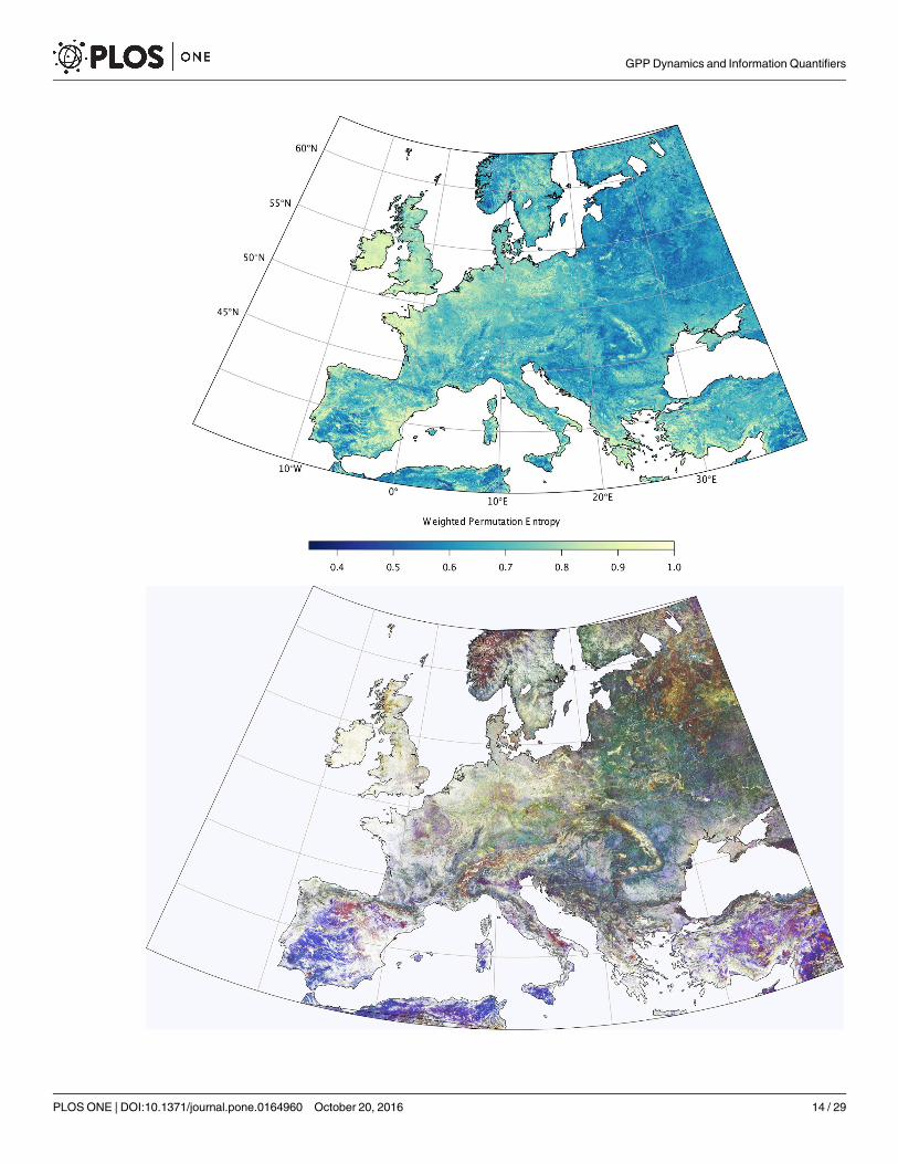
Continental-scalegradients in Information TheoryQuantifiers. ITQ from time seriesof vegetation activity proxies such as FAPAR show a large variety of spatial patterns from localto continental scales due to differences in vegetation type, land use, climate, and other factors.For example, the Weighted Permutation Entropy (Hw) for monthly FAPAR time series overEurope shows large spatial gradients that are mainly related to the regularity of the seasonalcycle in vegetation activity (Fig 3, upper panel). Western parts of the continent and manycoastal regions show rather high entropy values, e.g. over the British Isles, North-WesternFrance, and the Netherlands, indicating a relatively stochastic behaviour of the respective timeseries. On the other hand, (North-)Eastern parts of the continent, but also seasonally dryregions like the Iberian peninsula, Southern Italy and North Africa exhibit low entropy valuesand thus monthly time series appear to be predictable. However, in Fig 3 it becomes alreadyobvious that a quantification of entropy alone is not able to distinguish between climatologi-cally and ecologically well-separated regions such as Southern Spain and Eastern Europe (bothdisplaying low entropy).

Therefore, additional ITQ are needed and useful to distinguish further features in the timeseries, e.g. related to the separation of stochastic vs. deterministic processes [21]. Therefore, weexemplify the potential of combining several ITQ in the context of environmental time seriesin an RGB color image (Fig 3, bottom panel), where three ITQ (Weighted permutationentropy, statistical complexity, and Fisher Information) are encoded in the red, green, and bluechannel, respectively (Fig 3, bottom panel). This picture (Fig 3, bottom panel, see S3 Fig for ahigh-resolution version, maps of individual ITQ are available in S1 and S2 Figs) illustrates thatITQ indeed capture a large amount of structure in environmental time series: Continental-scale gradients are clearly visible, but now structurally distinct regions (e.g. Southern Spain vs.

GPP Dynamics and Information Quantifiers

PLOS ONE | DOI:10.1371/journal.pone.0164960 October 20, 2016 13 / 29

GPP Dynamics and Information Quantifiers

PLOS ONE | DOI:10.1371/journal.pone.0164960 October 20, 2016 14 / 29

Eastern Europe, see above) become well separated. Moreover, regional structures related toecosystem type, vegetation seasonality, and topography (e.g. mountain ranges) appear. Itshould be noted that the patterns and gradients obtained result from dynamical behaviour, i.e.quantify properties of vegetation in time, whereas the relation to other aspects like water avail-ability, soil type, climate zone, or topography is non trivial and they do not enter the calculationat all. This is a demonstration of the strength of the link between dynamical properties andenvironmental conditions for plant communities (the basis of plant biogeography). Theseresults thus highlight the potential of ITQ as indicators of ecological structure, and for model-data comparison exercises (see next subsection).

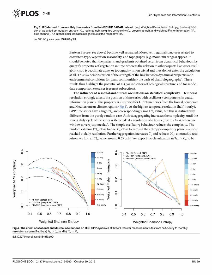
The influence of seasonal and diurnal oscillations on statistical complexity. Temporalresolution strongly affects the position of time series with oscillatory components in causalinformation planes. This property is illustrated for GPP time series from the boreal, temperateand Mediterranean climate regions (Fig 4). At the highest temporal resolution (half-hourly),GPP time series have a high Hw and correspondingly small Cw value, but this is distinctivelydifferent from the purely random case. At first, aggregating increases the complexity, until thestrong daily cycle of the series is ‘detected’ at a resolution of 6 hours (due to D = 4, when onewindow covers just one day). The simple oscillatory behaviour reduces the complexity. Therandom extreme (Hw close to one, Cw close to zero) in the entropy-complexity plane is almostreached at daily resolution. Further aggregation increases Cw and reduces Hw; at monthly reso-lution, we find an Hw value around 0.65 only. We expect the classification in Hw � Cw to be

Fig 3. ITQ derived from monthly time series from the JRC-TIP FAPAR dataset. (top) Weighted Permutation Entropy, (bottom) RGB

plot of weighted permutation entropy (Hw, red channel), weighted complexity (Cw, green channel), and weighted Fisher Information (Fw,

blue channel). An intense color indicates a high value of the respective ITQ.

doi:10.1371/journal.pone.0164960.g003

Fig 4. The effect of seasonal and diurnal oscillations on ITQ. GPP dynamics at three flux tower measurement sites from half-hourly to monthly

resolution as quantified by a) Hw � Cw, and b) Hw �Fw.

doi:10.1371/journal.pone.0164960.g004

GPP Dynamics and Information Quantifiers

PLOS ONE | DOI:10.1371/journal.pone.0164960 October 20, 2016 15 / 29

most sensitive in this region in the center of the plane, since the difference between upper andlower limit curves is largest here. Thus, the monthly scale seems to be especially suitable for thesubsequent regional assessment. It is not possible to further aggregate the series due to thelength requirements—but at 3 months resolution, the annual cycle would be found, andanother ‘loop’ in the diagram would be expected.

Similar to Hw � Cw, the position of a time series in the Shannon-Fisher plane (Hw � Fw)strongly depends on the temporal resolution (Fig 4). At the highest temporal resolution, theobserved, EC-based GPP time series has a high Hw ’ 0:95 and a very small Fisher information.Aggregation decreases entropy and increases Fw (Fig 4, upper part), until again the daily cycleof the series comes into reach at a resolution of 6 hours. Further aggregation increases entropyand decreases Fisher information, towards the “random corner” (Hw close to one, Fw close tozero) which is almost reached at daily and two-daily resolution. Aggregating further leads to amore and more steep increase in Fw, where the slope of this part of the curve resembles that ofthe k-noise shown in Fig 2.

Model-data comparison using ITQ

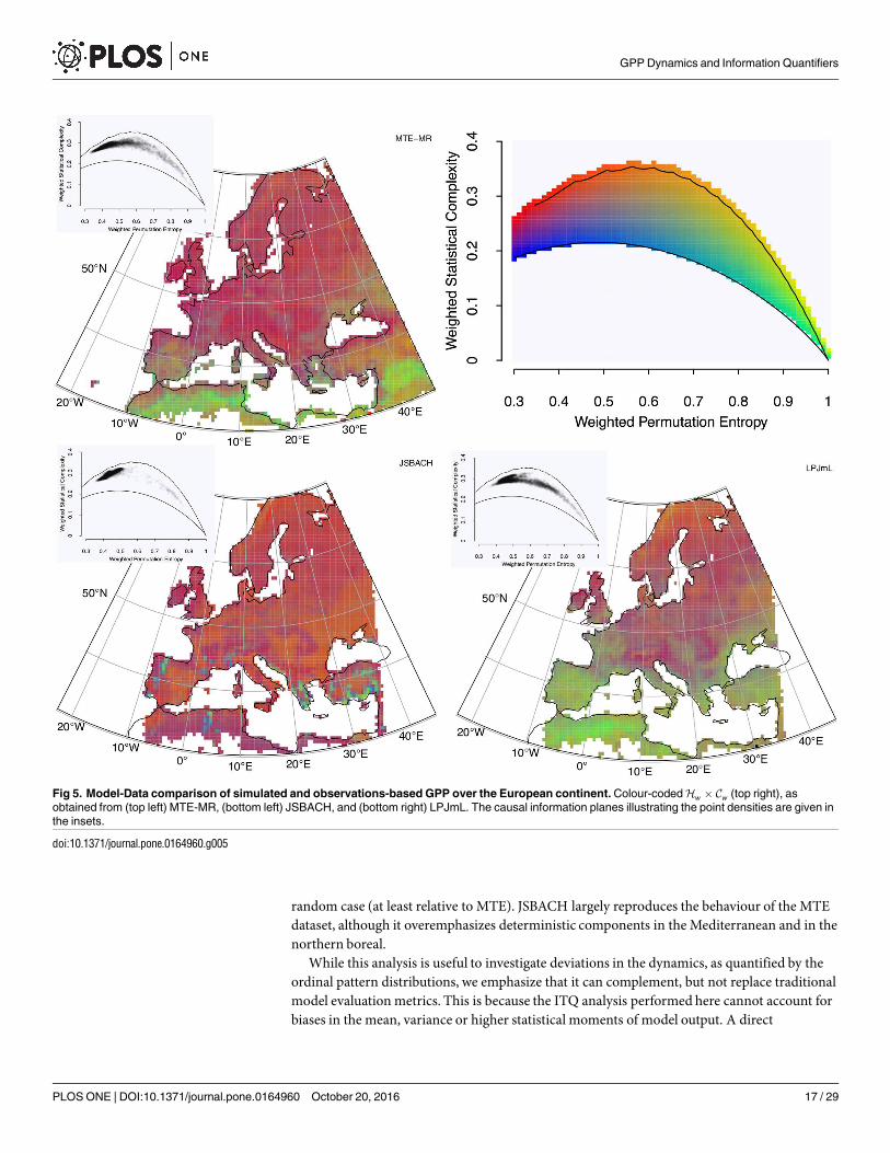
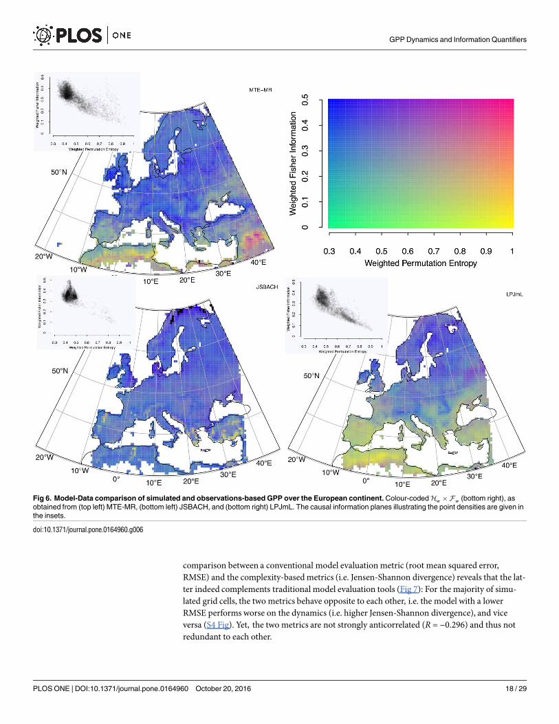
ITQ calculated from long-term GPP time series (1982-2011) at monthly resolution acrossEurope from two models and an observations-based product are shown in Fig 5 (Hw � Cw andFig 6 Hw � Fw), using a 2-dimensional colour scheme for visualization in a single map [80].The observations-based product (MTE reconstructions, upper panels) indicate large, compara-tively homogeneous regions across major biogeographical gradients, where the entropy of GPPtime series is intermediate and their complexity medium to high. In the Mediterranean and inNorth Africa, the entropy is higher and the complexity and Fisher Information lower.

In the context of this comparison, MTE results are considered as “surrogate observations”or benchmarking datasets to be reproduced by the land surface models—a typical scenario incarbon cycle research [81, 82]. Accepting this assumption for the sake of comparison, modelsare considered “realistic” if their output is close to the MTE results (Figs 5 and 6). The firstobservation is that JSBACH produces a spatially very homogeneous ITQ field, whereas LPJmLexhibits a pronounced North-South gradient. A striking difference between the models is thatJSBACH is more or less reproducing the ITQ from MTE, whereas LPJmL generates outputwhich appears with higher information content than MTE. However, in seasonally dry regionssuch as southern parts of the Iberian Peninsula and North Africa, MTE and LPJmL seem topoint in a similar direction towards higher entropy time series, whereas JSBACH does notshow this feature. Thus, in these regions LPJmL performs better. These patterns likewisebecome obvious when looking at the density of points in the planes (insets), where JSBACHhas much lower density in the high-entropy and low-complexity/low Fisher Informationregion than the observations; for LPJmL, the reverse holds true.

An interesting question in the context of model-data comparison using ITQ relates towhether the derived mismatch patterns (Figs 5 and 6) would be reproduced by traditionalmodel performance metrics (e.g. the root mean squared error, RMSE).

In Fig 7, colour-coded Jensen-Shannon divergences for the ordinal pattern distributionsbetween the observation dataset MTE-MR and either of the two models are visualized and canbe seen as an ITQ-based model performance metric. These maps demonstrate that JSBACHmodel output is rather close to the MTE-reconstructions in large parts of Central and EasternEurope, but shows some deviations in Scandinavia, North-West Russia, and Northern Africa.In contrast, LPJmL is in better agreement with the MTE in Scandinavia, but LPJmL deviatesfrom MTE in the Mediterranean and in several temperate European regions. Overall, LPJmL isthe model with higher entropy values (at the monthly time scale) having a bias towards the

GPP Dynamics and Information Quantifiers

PLOS ONE | DOI:10.1371/journal.pone.0164960 October 20, 2016 16 / 29

random case (at least relative to MTE). JSBACH largely reproduces the behaviour of the MTEdataset, although it overemphasizes deterministic components in the Mediterranean and in thenorthern boreal.

While this analysis is useful to investigate deviations in the dynamics, as quantified by theordinal pattern distributions, we emphasize that it can complement, but not replace traditionalmodel evaluation metrics. This is because the ITQ analysis performed here cannot account forbiases in the mean, variance or higher statistical moments of model output. A direct

Fig 5. Model-Data comparison of simulated and observations-based GPP over the European continent. Colour-coded Hw � Cw (top right), as

obtained from (top left) MTE-MR, (bottom left) JSBACH, and (bottom right) LPJmL. The causal information planes illustrating the point densities are given in

the insets.

doi:10.1371/journal.pone.0164960.g005

GPP Dynamics and Information Quantifiers

PLOS ONE | DOI:10.1371/journal.pone.0164960 October 20, 2016 17 / 29

comparison between a conventional model evaluation metric (root mean squared error,RMSE) and the complexity-based metrics (i.e. Jensen-Shannon divergence) reveals that the lat-ter indeed complements traditional model evaluation tools (Fig 7): For the majority of simu-lated grid cells, the two metrics behave opposite to each other, i.e. the model with a lowerRMSE performs worse on the dynamics (i.e. higher Jensen-Shannon divergence), and viceversa (S4 Fig). Yet, the two metrics are not strongly anticorrelated (R = −0.296) and thus notredundant to each other.

Fig 6. Model-Data comparison of simulated and observations-based GPP over the European continent. Colour-coded Hw �Fw (bottom right), as

obtained from (top left) MTE-MR, (bottom left) JSBACH, and (bottom right) LPJmL. The causal information planes illustrating the point densities are given in

the insets.

doi:10.1371/journal.pone.0164960.g006

GPP Dynamics and Information Quantifiers

PLOS ONE | DOI:10.1371/journal.pone.0164960 October 20, 2016 18 / 29

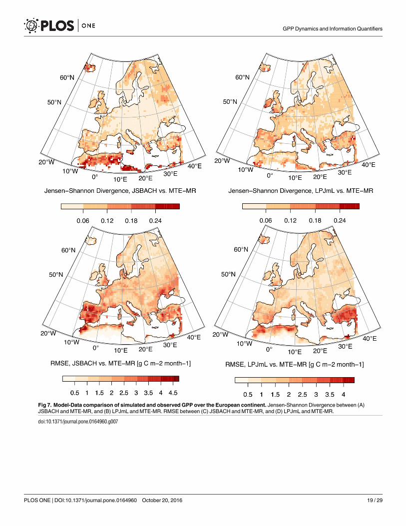
Fig 7. Model-Data comparison of simulated and observed GPP over the European continent. Jensen-Shannon Divergence between (A)

JSBACH and MTE-MR, and (B) LPJmL and MTE-MR. RMSE between (C) JSBACH and MTE-MR, and (D) LPJmL and MTE-MR.

doi:10.1371/journal.pone.0164960.g007

GPP Dynamics and Information Quantifiers

PLOS ONE | DOI:10.1371/journal.pone.0164960 October 20, 2016 19 / 29

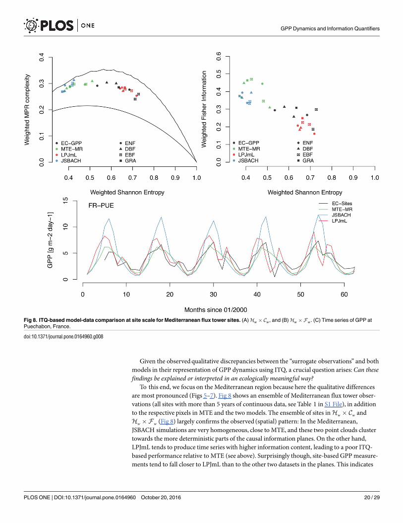
Given the observed qualitative discrepancies between the “surrogate observations” and bothmodels in their representation of GPP dynamics using ITQ, a crucial question arises:Can thesefindings be explained or interpreted in an ecologically meaningful way?

To this end, we focus on the Mediterranean region because here the qualitative differencesare most pronounced (Figs 5–7). Fig 8 shows an ensemble of Mediterranean flux tower obser-vations (all sites with more than 5 years of continuous data, see Table 1 in S1 File), in additionto the respective pixels in MTE and the two models. The ensemble of sites in Hw � Cw andHw � Fw (Fig 8) largely confirms the observed (spatial) pattern: In the Mediterranean,JSBACH simulations are very homogeneous, close to MTE, and these two point clouds clustertowards the more deterministic parts of the causal information planes. On the other hand,LPJmL tends to produce time series with higher information content, leading to a poor ITQ-based performance relative to MTE (see above). Surprisingly though, site-based GPP measure-ments tend to fall closer to LPJmL than to the other two datasets in the planes. This indicates

Fig 8. ITQ-based model-data comparison at site scale for Mediterranean flux tower sites. (A) Hw � Cw, and (B) Hw � Fw. (C) Time series of GPP at

Puechabon, France.

doi:10.1371/journal.pone.0164960.g008

GPP Dynamics and Information Quantifiers

PLOS ONE | DOI:10.1371/journal.pone.0164960 October 20, 2016 20 / 29

that the observations-based MTE product (and JSBACH) do not necessarily match the site-level GPP measurements from an ITQ perspective. However, a ‘process-oriented’ interpreta-tion of these ITQ-based patterns and discrepancies is feasible, considering, for example, themonthly GPP time series of an evergreen broadleaf forest site (Puechabon, France, Fig 8, bot-tom panel): Here, MTE and JSBACH indicate a very simple seasonal oscillation with only one(summer) peak per season. In contrast, flux tower measurements and LPJmL exhibit a two-peaked seasonal structure, with an early summer peak, subsequent GPP reduction due to waterlimitation, followed by a (smaller) autumn peak once water limitation ceases. Hence, in themodel-data comparison presented above, ITQ readily diagnose these two contrasting dynam-ics, which can thus be used as a starting point to improve or optimize models and observa-tions-based datasets.

In summary, these results show that model evaluation and improvement based solely onabsolute or relative error metrics could be misleading if the dynamics are misrepresented in themodel; in contrast a joint consideration of a variety of benchmarking metrics might provideuseful hints to scrutinizing various aspects of model behaviour.

Global analysis of land surface models

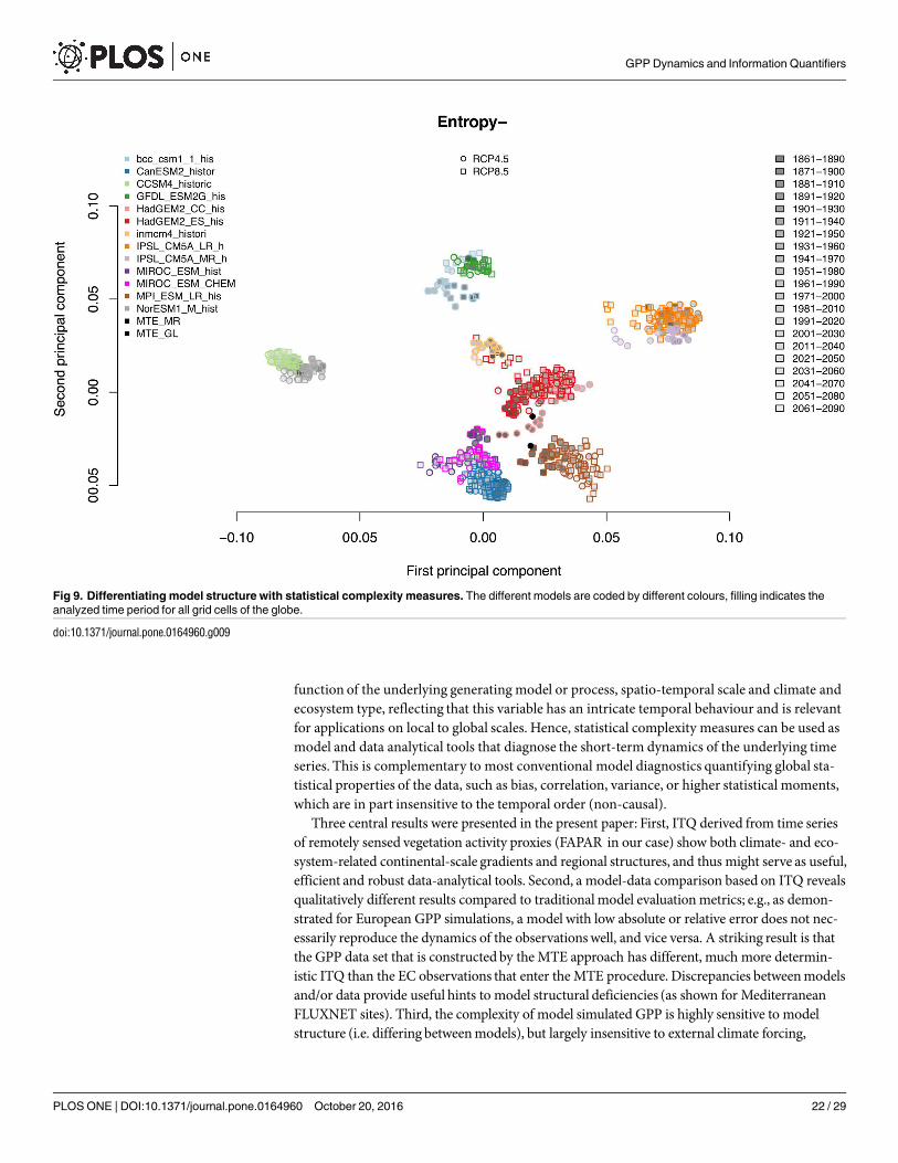
The CMIP5 runs allow a detailed evaluation of the relative importance of the model choice andthe scenario used (cf. Table 2 in S1 File). Global maps of the Weighted Permutation Entropy(S6 Fig) and the causal information planes for one of the 30-years periods and all 59 modelruns are shown in S7 and S8 Figs. These plots show a large diversity of patterns and point den-sities in Hw � Cw across the runs. Some of the models extend over the whole entropy range,others are more constrained to higher entropy values. Although looking quite similar at firstglance for most of the 59 model simulations, it is obvious that the local density of points israther different between them. None of the simulations is very close to the upper limit curve,i.e. do not achieve the highest complexity possible, which would be the realm of deterministicdynamical systems. This might be explained by the fact that these models are not autonomousdynamical systems, but driven by stochastic drivers such as precipitation. In Hw � Fw, manysimulations exhibit a “fork” structure, or a separation of the values into (at least) two different“curves” with two different slopes (S8 Fig). The width of the point clouds around these “curves”is, however, rather different between the simulations. Global maps of the Weighted Permuta-tion Entropy confirm that different models indeed show considerable differences in the simu-lated dynamics of GPP across various regions of the globe (S6 Fig). Using the rasteringpresented in the Methods section, we performed a PCA of the point clouds. The result for thefirst two dimensions is given by Fig 9. This figure shows that the entropy and Fisher informa-tion measures separate models according to model structural properties, and not scenarios,which is the core result of this section. Note that in all cases where clusters contain points ofdifferent colours, the colour-encoded models are actually variants of each other, for example,differing in spatial resolution or with or without a module for atmospheric chemistry. The clas-sification is not sensitive to the two scenarios, which were identical for all models. The linear orbow-shaped structures of the points for some of the models indicate a systematic developmentduring the simulation period.

Conclusions

The main intention of the current paper was to test the usefulness of Information TheoryQuantifiers as tools for data analysis and model benchmarking in the environmental sciences,and thus to reach a wider dissemination of these tools. Time series of simulated and observedGPP as a key ecosystem variable were investigated to show that the dynamics varies as a

GPP Dynamics and Information Quantifiers

PLOS ONE | DOI:10.1371/journal.pone.0164960 October 20, 2016 21 / 29

function of the underlying generating model or process, spatio-temporal scale and climate andecosystem type, reflecting that this variable has an intricate temporal behaviour and is relevantfor applications on local to global scales. Hence, statistical complexity measures can be used asmodel and data analytical tools that diagnose the short-term dynamics of the underlying timeseries. This is complementary to most conventional model diagnostics quantifying global sta-tistical properties of the data, such as bias, correlation, variance, or higher statistical moments,which are in part insensitive to the temporal order (non-causal).

Three central results were presented in the present paper: First, ITQ derived from time seriesof remotely sensed vegetation activity proxies (FAPAR in our case) show both climate- and eco-system-related continental-scale gradients and regional structures, and thus might serve as useful,efficient and robust data-analytical tools. Second, a model-data comparison based on ITQ revealsqualitatively different results compared to traditional model evaluation metrics; e.g., as demon-strated for European GPP simulations, a model with low absolute or relative error does not nec-essarily reproduce the dynamics of the observations well, and vice versa. A striking result is thatthe GPP data set that is constructed by the MTE approach has different, much more determin-istic ITQ than the EC observations that enter the MTE procedure. Discrepancies between modelsand/or data provide useful hints to model structural deficiencies (as shown for MediterraneanFLUXNET sites). Third, the complexity of model simulated GPP is highly sensitive to modelstructure (i.e. differing between models), but largely insensitive to external climate forcing,

Fig 9. Differentiating model structure with statistical complexity measures. The different models are coded by different colours, filling indicates the

analyzed time period for all grid cells of the globe.

doi:10.1371/journal.pone.0164960.g009

GPP Dynamics and Information Quantifiers

PLOS ONE | DOI:10.1371/journal.pone.0164960 October 20, 2016 22 / 29

atmospheric greenhouse gas concentrations or land use changes, as demonstrated for global- andbiome-scale GPP simulations from the CMIP5 archive. These results highlight the benefits ofmodel benchmarking and evaluation against a variety of model evaluation metrics, includingmodel structural diagnostics such as the ITQ presented here.

ITQ allow a ranking of models according to their ability to reproduce the observed dynam-ical behaviour within the time span given by the embedding dimension and the delay parame-ter. The crucial limiting factor for this time span is the length of the time series. In the future,the complexity indicators could serve as objective functions to improve model performance,e.g. in an iterative or machine-learning setting to find optimal parameter sets or model struc-tures (Ilie et al., submitted to Geoscientific Model Development) or in a data assimilation system(see e.g. [83]). In general terms, the methods employed here analyze and compare data sets, notmodels. They are close to non-parametric—the choice of the embedding dimension is dictatedby the length of the time series—and do not make any specific assumptions about properties ofthe data, statistical or otherwise. Our results indicate that for land surface models, it is likelynot sufficient to change the parameters of the model to reproduce the observed behaviour;rather, the model structure has to be revised, since the same model structure produces similarpatterns independent of e.g. their initialization and the details of the parametrization.

Finally, a broad range of future applications of Information Theory Quantifiers in environ-mental science is conceivable: These could consist of efficiently diagnosing satellite datastreams of very high spatio-temporal resolution in an increasingly data-rich era, as well as touse statistical complexity of environmental variables for classification purposes. Therefore, wepropose that these tools could be taken up more widely by the community for model evaluationand benchmarking activities.

Supporting Information

S1 Fig. Weighted statistical complexity for the JRC-TIP FPAR dataset.(PDF)

S2 Fig. Weighted Fisher Information for the JRC-TIP FPAR dataset.(PDF)

S3 Fig. High-resolution version of Fig 3 (bottom panel) in the main text.(PDF)

S4 Fig. ITQ-based and RMSE-basedmodel comparison of JSBACH and LPJmL vs. MTE.(left) Jensen-Shannon Divergence, and (right) RMSE.(PDF)

S5 Fig. ITQ’s for temperate and boreal FLUXNET sites. (top left) Boreal sites, Hw � Cw, and(top right) boreal sites Hw � Fw. (bottom left) Temperate sites, Hw � Cw, and (bottom right)temperate sites, Hw � Fw.(PDF)

S6 Fig. Globalmaps of theWeighted Permutation Entropy of GPP fluxes across 59 CMIP5models and simulations for all land grid cells. Plots are illustrative for the 30-yr period 1981-2010.(PDF)

S7 Fig.Hw � Cw of GPP fluxes across 59 CMIP5 models and simulations for all land gridcells. Plots are illustrative for the 30-yr period 1981-2010.(JPG)

GPP Dynamics and Information Quantifiers

PLOS ONE | DOI:10.1371/journal.pone.0164960 October 20, 2016 23 / 29

S8 Fig.Hw � Fw of GPP fluxes across 59 CMIP5models and simulations for all land gridcells. Plots are illustrative for the 30-yr period 1981-2010.(JPG)

S1 File. Supporting Information file that contains additional Text and Tables.(PDF)

S1 Code. Supporting CodeTutorial that introduces the R-package on Statistical Complex-ity (“statcomp”) and allows to reproduce Figs 1 and 2.(R)

Acknowledgments

We thank Kirsten Thonicke and Susanne Rolinski for providing LPJmL model output, Chris-tian Beer for providing JSBACH results, data management and the modelling protocol. Fur-thermore, we thank Anja Rammig and Markus Reichstein for comments and discussions. S.S.is grateful to the ‘German National Academic Foundation’ (Studienstiftung des DeutschenVolkes) for support and the International Max Planck Research School for Global Biogeo-chemical Cycles (IMPRS-gBGC) for training. H.L. is grateful to the hospitality at the Institutode Física, Universidade Federal de Alagoas in Maceió, Brazil, and also to the guest researcherfunding provided by the Conselho Nacional de Desenvolvimento Científico e Tecnológico(CNPq, fellowship no. 310003/2016-4) during a sabbatical stay. O.A.R. acknowledges supportfrom Consejo Nacional de Investigaciones Científicas y Técnicas (CONICET), Argentina. S.S.,F.G., and M.D.M. thank the European Space agency for funding the STSE project CAB-LAB; S.S., F.G., and M.D.M. are also grateful to the European Commission for funding the BACI proj-ect; grant agreement No 640176. The JRC-TIP FAPAR product based on MODIS broadbandalbedo observations was provided by The Inversion Lab and the Joint Research Centre of theEuropean Commission, and we thank Michael Voßbeck, Bernhard Pinty, and Nadine Gobronfor making the dataset available. This work used eddy covariance data acquired by the FLUX-NET community and in particular by the following networks: CarboEuropeIP, CarboItaly,CarboMont, GreenGrass. We acknowledge the financial support to the eddy covariance dataharmonization provided by CarboEuropeIP, FAO-GTOS-TCO, iLEAPS, Max Planck Institutefor Biogeochemistry, National Science Foundation, University of Tuscia, Université Laval,Environment Canada and US Department of Energy and the database development and tech-nical support from Berkeley Water Center, Lawrence Berkeley National Laboratory, MicrosoftResearch eScience, Oak Ridge National Laboratory, University of California—Berkeley and theUniversity of Virginia. We acknowledge the World Climate Research Programme’s WorkingGroup on Coupled Modelling, which is responsible for CMIP, and we thank the climate model-ling groups (listed in Table 2 in S1 File) for producing and making available their model out-put. For CMIP the U.S. Department of Energy’s Program for Climate Model Diagnosis andIntercomparison provides coordinating support and led development of software infrastruc-ture in partnership with the Global Organization for Earth System Science Portals.

Author Contributions

Conceptualization: SS HL MDM MH OAR.

Formal analysis: SS HL.

Funding acquisition:MDM.

Investigation: MDM FG TK.

GPP Dynamics and Information Quantifiers

PLOS ONE | DOI:10.1371/journal.pone.0164960 October 20, 2016 24 / 29

Methodology:SS HL.

Resources:MDM TK.

Software: SS TK HL OAR.

Supervision:MDM HL.

Validation: SS MDM PB FG.

Visualization: TK SS.

Writing – original draft: SS HL MH OAR.

Writing – review& editing: SS HL.

References1. Ciais P, Sabine C, Bala G, Bopp L, Brovkin V, Canadell J, et al. Carbon and other biogeochemical

cycles. In: Climate Change 2013: The Physical Science Basis. Contribution of Working Group I to the

Fifth Assessment Report of the Intergovernmental Panel on Climate Change. Cambridge University

Press; 2014. p. 465–570.

2. Eyring V, Righi M, Evaldsson M, Lauer A, Wenzel S, Jones C, et al. ESMValTool (v1.0): a community

diagnostic and performance metrics tool for routine evaluation of Earth System Models in CMIP. Geos-

cientific Model Development. 2016; 9:1747–1802. doi: 10.5194/gmd-9-1747-2016

3. Taylor KE, Stouffer RJ, Meehl GA. An overview of CMIP5 and the experiment design. Bulletin of the

American Meteorological Society. 2012; 93(4):485–498. doi: 10.1175/BAMS-D-11-00094.1

4. Kelley D, Prentice IC, Harrison S, Wang H, Simard M, Fisher J, et al. A comprehensive benchmarking

system for evaluating global vegetation models. Biogeosciences. 2013; 10:3313–3340. doi: 10.5194/

bg-10-3313-2013

5. Abramowitz G. Towards a benchmark for land surface models. Geophysical Research Letters. 2005;

32(22). doi: 10.1029/2005GL024419

6. Gupta HV, Clark MP, Vrugt JA, Abramowitz G, Ye M. Towards a comprehensive assessment of model

structural adequacy. Water Resources Research. 2012; 48(8). doi: 10.1029/2011WR011044

7. Abramowitz G. Towards a public, standardized, diagnostic benchmarking system for land surface

models. Geoscientific Model Development. 2012; 5(3):819–827. doi: 10.5194/gmd-5-819-2012

8. Luo YQ, Randerson JT, Abramowitz G, Bacour C, Blyth E, Carvalhais N, et al. A framework for bench-

marking land models. Biogeosciences. 2012; 9(10):3857–3874. doi: 10.5194/bg-9-3857-2012

9. Best M, Abramowitz G, Johnson H, Pitman A, Balsamo G, Boone A, et al. The plumbing of land surface

models: benchmarking model performance. Journal of Hydrometeorology. 2015; (2015: ). doi: 10.

1175/JHM-D-14-0158.1

10. Carvalhais N, Forkel M, Khomik M, Bellarby J, Jung M, Migliavacca M, et al. Global covariation of car-

bon turnover times with climate in terrestrial ecosystems. Nature. 2014; 514(7521):213–217. doi: 10.

1038/nature13731 PMID: 25252980

11. Grimm V, Railsback SF. Pattern-oriented modelling: a ‘multi-scope’ for predictive systems ecology.

Phil Trans R Soc B. 2012; 367(1586):298–310. doi: 10.1098/rstb.2011.0180 PMID: 22144392

12. Reichstein M, Beer C. Soil respiration across scales: the importance of a model–data integration

framework for data interpretation. Journal of Plant Nutrition and Soil Science. 2008; 171(3):344–354.

doi: 10.1002/jpln.200700075

13. Reichstein M, Mahecha MD, Ciais P, Seneviratne SI, Blyth EM, Carvalhais N, et al. Elk–testing cli-

mate–carbon cycle models: a case for pattern–oriented system analysis. iLEAPS Newsletter. 2011;

11:14–21.

14. Mahecha MD, Reichstein M, Jung M, Seneviratne SI, Zaehle S, Beer C, et al. Comparing observations

and process-based simulations of biosphere-atmosphere exchanges on multiple timescales. Journal

of Geophysical Research: Biogeosciences. 2010; 115(G2). doi: 10.1029/2009JG001016

15. Chapin SF III, Matson P P A andVitousek. Principles of Terrestrial Ecosystem Ecology. 2nd ed.

Springer; 2011.

16. Baldocchi D, Falge E, Gu L, Olson R, Hollinger D, Running S, et al. FLUXNET: A new tool to study the

temporal and spatial variability of ecosystem-scale carbon dioxide, water vapor, and energy flux

GPP Dynamics and Information Quantifiers

PLOS ONE | DOI:10.1371/journal.pone.0164960 October 20, 2016 25 / 29

densities. Bulletin of the American Meteorological Society. 2001; 82(11):2415–2434. doi: 10.1175/

1520-0477(2001)082%3C2415:FANTTS%3E2.3.CO;2

17. Moss RH, Edmonds JA, Hibbard KA, Manning MR, Rose SK, Van Vuuren DP, et al. The next genera-

tion of scenarios for climate change research and assessment. Nature. 2010; 463(7282):747–756. doi:

10.1038/nature08823 PMID: 20148028

18. Reichstein M, Bahn M, Ciais P, Frank D, Mahecha MD, Seneviratne SI, et al. Climate extremes and

the carbon cycle. Nature. 2013; 500(7462):287–295. doi: 10.1038/nature12350 PMID: 23955228

19. Zscheischler J, Reichstein M, Harmeling S, Rammig A, Tomelleri E, Mahecha MD. Extreme events in

gross primary production: a characterization across continents. Biogeosciences. 2014; 11(11):2909–

2924. doi: 10.5194/bg-11-2909-2014

20. Gray RM. Entropy and information theory. Springer Science & Business Media; 2011.

21. Rosso OA, Larrondo H, Martin M, Plastino A, Fuentes M. Distinguishing noise from chaos. Physical

review letters. 2007; 99(15):154102. doi: 10.1103/PhysRevLett.99.154102 PMID: 17995170

22. Bandt C, Pompe B. Permutation entropy: a natural complexity measure for time series. Physical review

letters. 2002; 88(17):174102. doi: 10.1103/PhysRevLett.88.174102 PMID: 12005759

23. Hauhs M, Lange H. Classification of Runoff in Headwater Catchments: A Physical Problem? Geogra-

phy Compass. 2008; 2(1):235–254. doi: 10.1111/j.1749-8198.2007.00075.x

24. Shannon CE. A mathematical theory of communication. Bell Syst Technol J. 1948; 27:379–423. doi:

10.1002/j.1538-7305.1948.tb01338.x

25. Frieden BR. Science from Fisher information: a unification. Cambridge University Press; 2004.

26. Brissaud JB. The meanings of entropy. Entropy. 2005; 7(1):68–96. doi: 10.3390/e7010068

27. Kantz H, Kurths J, Mayer-Kress G. Nonlinear analysis of physiological data. Springer Science & Busi-

ness Media; 2012.

28. Feldman DP, McTague CS, Crutchfield JP. The organization of intrinsic computation: Complexity-

entropy diagrams and the diversity of natural information processing. Chaos: An Interdisciplinary Jour-

nal of Nonlinear Science. 2008; 18(4):043106. doi: 10.1063/1.2991106

29. Lamberti P, Martin M, Plastino A, Rosso O. Intensive entropic non-triviality measure. Physica A: Statis-

tical Mechanics and its Applications. 2004; 334(1):119–131. doi: 10.1016/j.physa.2003.11.005

30. Lopez-Ruiz R, Mancini HL, Calbet X. A statistical measure of complexity. Physics Letters A. 1995; 209

(5-6):321–326. doi: 10.1016/0375-9601(95)00867-5

31. Martin M, Plastino A, Rosso O. Statistical complexity and disequilibrium. Physics Letters A. 2003; 311

(2):126–132. doi: 10.1016/S0375-9601(03)00491-2

32. Grosse I, Bernaola-Galvan P, Carpena P, Roman-Roldan R, Oliver J, Stanley HE. Analysis of symbolic

sequences using the Jensen-Shannon divergence. Physical Review E. 2002; 65(4):041905. doi: 10.

1103/PhysRevE.65.041905 PMID: 12005871

33. Martin M, Plastino A, Rosso OA. Generalized statistical complexity measures: Geometrical and analyt-

ical properties. Physica A: Statistical Mechanics and its Applications. 2006; 369(2):439–462. doi: 10.

1016/j.physa.2005.11.053

34. Olivares F, Plastino A, Rosso OA. Contrasting chaos with noise via local versus global information

quantifiers. Physics Letters A. 2012; 376(19):1577–1583. doi: 10.1016/j.physleta.2012.03.039

35. Olivares F, Plastino A, Rosso OA. Ambiguities in Bandt–Pompe’s methodology for local entropic quan-

tifiers. Physica A: Statistical Mechanics and its Applications. 2012; 391(8):2518–2526. doi: 10.1016/j.

physa.2011.12.033

36. Keller K, Sinn M. Ordinal analysis of time series. Physica A: Statistical Mechanics and its Applications.

2005; 356(1):114–120. doi: 10.1016/j.physa.2005.05.022

37. Rosso OA, Masoller C. Detecting and quantifying temporal correlations in stochastic resonance via

information theory measures. European Physical Journal B. 2009; 69(1):37–43. doi: 10.1140/epjb/

e2009-00146-y

38. Saco PM, Carpi LC, Figliola A, Serrano E, Rosso OA. Entropy analysis of the dynamics of El Niño/

Southern Oscillation during the Holocene. Physica A: Statistical Mechanics and its Applications. 2010;

389(21):5022–5027. doi: 10.1016/j.physa.2010.07.006

39. Zanin M, Zunino L, Rosso OA, Papo D. Permutation entropy and its main biomedical and econophy-

sics applications: a review. Entropy. 2012; 14(8):1553–1577. doi: 10.3390/e14081553

40. Fadlallah B, Chen B, Keil A, Prıncipe J. Weighted-permutation entropy: A complexity measure for time

series incorporating amplitude information. Physical Review E. 2013; 87(2):022911. doi: 10.1103/

PhysRevE.87.022911 PMID: 23496595

GPP Dynamics and Information Quantifiers

PLOS ONE | DOI:10.1371/journal.pone.0164960 October 20, 2016 26 / 29

41. Renyi A. On measures of information and entropy. In: Proceedings of the fourth Berkeley Symposium

on Mathematics, Statistics and Probability 1960; 1961. p. 547–561. Available from: http://digitalassets.

lib.berkeley.edu/math/ucb/text/math_s4_v1_article-27.pdf

42. Rosso OA, De Micco L, Plastino A, Larrondo HA. Info-quantifiers’ map-characterization revisited. Phy-

sica A: Statistical Mechanics and its Applications. 2010; 389(21):4604–4612. doi: 10.1016/j.physa.

2010.06.055

43. Kowalski A, Martın M, Plastino A, Rosso O. Fisher information description of the classical–quantal

transition. Physica A: Statistical Mechanics and its Applications. 2011; 390(12):2435–2441. doi: 10.

1016/j.physa.2011.02.009

44. De Micco L, Fernandez JG, Larrondo HA, Plastino A, Rosso O. Sampling period, statistical complexity,

and chaotic attractors. Physica A: Statistical Mechanics and its Applications. 2012; 391(8):2564–2575.

doi: 10.1016/j.physa.2011.12.042

45. Lange H, Rosso OA, Hauhs M. Ordinal pattern and statistical complexity analysis of daily stream flow

time series. The European Physical Journal Special Topics. 2013; 222(2):535–552. doi: 10.1140/epjst/

e2013-01858-3

46. Serinaldi F, Zunino L, Rosso OA. Complexity–entropy analysis of daily stream flow time series in the

continental United States. Stochastic Environmental Research and Risk Assessment. 2014; 28

(7):1685–1708. doi: 10.1007/s00477-013-0825-8

47. Montani F, Deleglise EB, Rosso OA. Efficiency characterization of a large neuronal network: A causal

information approach. Physica A: Statistical Mechanics and its Applications. 2014; 401:58–70. doi: 10.

1016/j.physa.2013.12.053

48. Montani F, Rosso OA. Entropy-Complexity Characterization of Brain Development in Chickens.

Entropy. 2014; 16(8):4677–4692. doi: 10.3390/e16084677

49. Montani F, Rosso OA, Matias FS, Bressler SL, Mirasso CR. A symbolic information approach to deter-

mine anticipated and delayed synchronization in neuronal circuit models. Phil Trans R Soc A. 2015;

373(2056):20150110. doi: 10.1098/rsta.2015.0110 PMID: 26527818

50. Montani F, Baravalle R, Montangie L, Rosso OA. Causal information quantification of prominent

dynamical features of biological neurons. Phil Trans R Soc A. 2015; 373(2056):20150109. doi: 10.

1098/rsta.2015.0109 PMID: 26527819

51. Aquino A, Cavalcante TS, Almeida ES, Frery AC, Rosso OA. Characterization of vehicle behavior with

information theory. European Physical Journal B:. 2015; 88:257. doi: 10.1140/epjb/e2015-60384-x

52. Kowalski A, Martın M, Plastino A, Rosso O. Bandt–Pompe approach to the classical-quantum transi-

tion. Physica D: Nonlinear Phenomena. 2007; 233(1):21–31. doi: 10.1016/j.physd.2007.06.015

53. Bariviera AF, Guercio MB, Martinez LB, Rosso OA. The (in) visible hand in the Libor market: an infor-

mation theory approach. The European Physical Journal B. 2015; 88(8):1–9. doi: 10.1140/epjb/e2015-

60410-1

54. Bariviera AF, Guercio MB, Martinez LB, Rosso OA. A permutation information theory tour through dif-

ferent interest rate maturities: the Libor case. Phil Trans R Soc A. 2015; 373(2056):20150119. doi: 10.

1098/rsta.2015.0119 PMID: 26527817

55. Bandt C. Ordinal time series analysis. Ecological Modelling. 2005; 182(3):229–238. doi: 10.1016/j.

ecolmodel.2004.04.003

56. Rosso O, Carpi LC, Saco PM, Ravetti MG, Plastino A, Larrondo HA. Causality and the entropy–com-

plexity plane: Robustness and missing ordinal patterns. Physica A: Statistical Mechanics and its Appli-

cations. 2012; 391(1):42–55. doi: 10.1016/j.physa.2011.07.030

57. Rosso O, Carpi L, Saco P, Ravetti MG, Larrondo H, Plastino A. The Amigo paradigm of forbidden/

missing patterns: a detailed analysis. The European Physical Journal B. 2012; 85(12):1–12. doi: 10.

1140/epjb/e2012-30307-8

58. Zunino L, Soriano MC, Fischer I, Rosso OA, Mirasso CR. Permutation-information-theory approach to

unveil delay dynamics from time-series analysis. Physical Review E. 2010; 82(4):046212. doi: 10.

1103/PhysRevE.82.046212 PMID: 21230370

59. Soriano MC, Zunino L, Rosso O, Fischer I, Mirasso CR, et al. Time scales of a chaotic semiconductor

laser with optical feedback under the lens of a permutation information analysis. Quantum Electronics,

IEEE Journal of. 2011; 47(2):252–261. doi: 10.1109/JQE.2010.2078799

60. Zunino L, Soriano MC, Rosso OA. Distinguishing chaotic and stochastic dynamics from time series by

using a multiscale symbolic approach. Physical Review E. 2012; 86(4):046210. doi: 10.1103/

PhysRevE.86.046210 PMID: 23214666

61. De Micco L, Gonzalez C, Larrondo H, Martin M, Plastino A, Rosso O. Randomizing nonlinear maps via

symbolic dynamics. Physica A: Statistical Mechanics and its Applications. 2008; 387(14):3373–3383.

doi: 10.1016/j.physa.2008.02.037

GPP Dynamics and Information Quantifiers

PLOS ONE | DOI:10.1371/journal.pone.0164960 October 20, 2016 27 / 29

62. De Micco L, Larrondo H, Plastino A, Rosso O. Quantifiers for randomness of chaotic pseudo-random

number generators. Philosophical Transactions of the Royal Society of London A: Mathematical, Phys-

ical and Engineering Sciences. 2009; 367(1901):3281–3296. doi: 10.1098/rsta.2009.0075

63. Ribeiro HV, Zunino L, Lenzi EK, Santoro PA, Mendes RS. Complexity-entropy causality plane as a

complexity measure for two-dimensional patterns. PloS one. 2012; 7(8):e40689. doi: 10.1371/journal.

pone.0040689 PMID: 22916097

64. Re MA, Azad RK. Generalization of Entropy Based Divergence Measures for Symbolic Sequence

Analysis. PLoS ONE. 2014; 9(4):1–11. doi: 10.1371/journal.pone.0093532

65. Pinty B, Clerici M, Andredakis I, Kaminski T, Taberner M, Verstraete M, et al. Exploiting the MODIS

albedos with the Two-stream Inversion Package (JRC-TIP): 2. Fractions of transmitted and absorbed

fluxes in the vegetation and soil layers. Journal of Geophysical Research: Atmospheres. 2011; 116

(D9). doi: 10.1029/2010JD015373

66. Zscheischler J, Orth R, Seneviratne SI. A submonthly database for detecting changes in vegetation-

atmosphere coupling. Geophysical Research Letters. 2015; 42(22):9816–9824. doi: 10.1002/

2015GL066563

67. Gobron N, Belward A, Pinty B, Knorr W. Monitoring biosphere vegetation 1998–2009. Geophysical

Research Letters. 2010; 37(15). doi: 10.1029/2010GL043870

68. Kaminski T, Pinty B, Voßbeck M, Lopatka M, Gobron N, Robustelli M. Consistent EO Land Surface

Products including Uncertainty Estimates. Biogeosciences Discussions. 2016; 2016:1–28. doi: 10.

5194/bg-2016-310

69. Reichstein M, Falge E, Baldocchi D, Papale D, Aubinet M, Berbigier P, et al. On the separation of net

ecosystem exchange into assimilation and ecosystem respiration: review and improved algorithm.

Global Change Biology. 2005; 11(9):1424–1439. doi: 10.1111/j.1365-2486.2005.001002.x

70. Jung M, Reichstein M, Margolis HA, Cescatti A, Richardson AD, Arain MA, et al. Global patterns of

land-atmosphere fluxes of carbon dioxide, latent heat, and sensible heat derived from eddy covari-

ance, satellite, and meteorological observations. Journal of Geophysical Research: Biogeosciences

(2005–2012). 2011; 116(G3). doi: 10.1029/2010JG001566

71. Lasslop G, Reichstein M, Papale D, Richardson AD, Arneth A, Barr A, et al. Separation of net ecosys-

tem exchange into assimilation and respiration using a light response curve approach: critical issues

and global evaluation. Global Change Biology. 2010; 16(1):187–208. doi: 10.1111/j.1365-2486.2009.

02041.x

72. Sitch S, Smith B, Prentice IC, Arneth A, Bondeau A, Cramer W, et al. Evaluation of ecosystem dynam-

ics, plant geography and terrestrial carbon cycling in the LPJ dynamic global vegetation model. Global

Change Biology. 2003; 9(2):161–185. doi: 10.1046/j.1365-2486.2003.00569.x

73. Bondeau A, Smith PC, Zaehle S, Schaphoff S, Lucht W, Cramer W, et al. Modelling the role of agricul-

ture for the 20th century global terrestrial carbon balance. Global Change Biology. 2007; 13(3):679–

706. doi: 10.1111/j.1365-2486.2006.01305.x

74. Haxeltine A, Prentice IC. BIOME3: An equilibrium terrestrial biosphere model based on ecophysiologi-

cal constraints, resource availability, and competition among plant functional types. Global Biogeo-

chemical Cycles. 1996; 10(4):693–709. doi: 10.1029/96GB02344

75. Knorr W. Annual and interannual CO2 exchanges of the terrestrial biosphere: Process-based simula-

tions and uncertainties. Global Ecology and Biogeography. 2000; 9(3):225–252. doi: 10.1046/j.1365-

2699.2000.00159.x

76. Raddatz TJ, Reick CH, Knorr W, Kattge J, Roeckner E, Schnur R, et al. Will the tropical land biosphere

dominate the climate–carbon cycle feedback during the twenty-first century? Climate Dynamics. 2007;

29(6):565–574. doi: 10.1007/s00382-007-0247-8

77. Thum T, Raisanen P, Sevanto S, Tuomi M, Reick C, Vesala T, et al. Soil carbon model alternatives for

ECHAM5/JSBACH climate model: evaluation and impacts on global carbon cycle estimates. Journal

of Geophysical Research: Biogeosciences (2005–2012). 2011; 116(G2). doi: 10.1029/2010JG001612

78. Osmond C, Winter K, Ziegler H. Functional significance of different pathways of CO2 fixation in photo-

synthesis. In: Physiological plant ecology II. Springer; 1982. p. 479–547. doi: 10.1007/978-3-642-

68150-9_16

79. Beer C, Weber U, Tomelleri E, Carvalhais N, Mahecha M, Reichstein M. Harmonized European Long-

Term Climate Data for Assessing the Effect of Changing Temporal Variability on Land–Atmosphere

CO2 Fluxes*. Journal of Climate. 2014; 27(13):4815–4834. doi: 10.1175/JCLI-D-13-00543.1

80. Teuling AJ, Stockli R, Seneviratne SI. Bivariate colour maps for visualizing climate data. International

Journal of Climatology. 2011; 31(9):1408–1412. doi: 10.1002/joc.2153

GPP Dynamics and Information Quantifiers

PLOS ONE | DOI:10.1371/journal.pone.0164960 October 20, 2016 28 / 29

81. Piao S, Sitch S, Ciais P, Friedlingstein P, Peylin P, Wang X, et al. Evaluation of terrestrial carbon cycle

models for their response to climate variability and to CO2 trends. Global Change Biology. 2013; 19

(7):2117–2132. doi: 10.1111/gcb.12187 PMID: 23504870

82. Anav A, Friedlingstein P, Kidston M, Bopp L, Ciais P, Cox P, et al. Evaluating the land and ocean com-

ponents of the global carbon cycle in the CMIP5 Earth System Models. Journal of Climate. 2013; 26

(18):6801–6843. doi: 10.1175/JCLI-D-12-00417.1

83. Schurmann GJ, Kaminski T, Kostler C, Carvalhais N, Voßbeck M, Kattge J, et al. Constraining a land

surface model with multiple observations by application of the MPI-Carbon Cycle Data Assimilation

System. Geoscientific Model Development Discussions. 2016; 2016:1–24.

GPP Dynamics and Information Quantifiers

PLOS ONE | DOI:10.1371/journal.pone.0164960 October 20, 2016 29 / 29