Long gravitational-wave transients and associated detection strategiesfor a network of terrestrial interferometers

Eric Thrane,1,* Shivaraj Kandhasamy,1 Christian D. Ott,2 Warren G. Anderson,3 Nelson L. Christensen,4

Michael W. Coughlin,4 Steven Dorsher,1 Stefanos Giampanis,5,3 Vuk Mandic,1 Antonis Mytidis,6

Tanner Prestegard,1 Peter Raffai,7 and Bernard Whiting6

1School of Physics and Astronomy, University of Minnesota, Minneapolis, Minnesota 55455, USA2TAPIR, Caltech, Pasadena, California 91125

3University of Wisconsin-Milwaukee, Milwaukee, Wisconsin 532014Physics and Astronomy, Carleton College, Northfield, Minnesota 55057

5Albert-Einstein-Institut, Max-Planck-Institut fur Gravitationsphysik, D-30167 Hannover, Germany6Department of Physics, University of Florida, Gainsville, Florida 32611, USA

7Institute of Physics, Eotvos University, 1117 Budapest, Hungary(Received 9 December 2010; published 11 April 2011)

Searches for gravitational waves (GWs) traditionally focus on persistent sources (e.g., pulsars or the

stochastic background) or on transients sources (e.g., compact binary inspirals or core-collapse super-

novae), which last for time scales of milliseconds to seconds. We explore the possibility of long GW

transients with unknown waveforms lasting from many seconds to weeks. We propose a novel analysis

technique to bridge the gap between short OðsÞ ‘‘burst’’ analyses and persistent stochastic analyses. Our

technique utilizes frequency-time maps of GW strain cross power between two spatially separated

terrestrial GW detectors. The application of our cross power statistic to searches for GW transients is

framed as a pattern recognition problem, and we discuss several pattern-recognition techniques. We

demonstrate these techniques by recovering simulated GW signals in simulated detector noise. We also

recover environmental noise artifacts, thereby demonstrating a novel technique for the identification of

such artifacts in GW interferometers. We compare the efficiency of this framework to other techniques

such as matched filtering.

DOI: 10.1103/PhysRevD.83.083004 PACS numbers: 95.85.Sz, 95.30.Sf, 95.55.Ym

I. INTRODUCTION

Historically, searches for gravitational-wave (GW) tran-sients fall into one of two categories: searches for ‘‘bursts’’whose precise waveforms we cannot predict and searchesfor compact binary coalescences, whose waveforms can bepredicted (at least for the inspiral part). Typically, burstsearches focus on events with& 1 s durations and, indeed,there are many compelling models for short GW transients(see [1] and references therein).

In this paper, we put the spotlight on long GW transientswhose durations may range from many seconds to weeks.Astrophysical GW emission scenarios for long transientsexist (e.g., [2–5]), but their characteristics have not pre-viously been broadly addressed and no data-analysis strat-egy has been proposed for such events until now. (Inaddition to this work, see recent developments in [6].)Most of the GWemission models we consider are burstlikein the sense that the signal evolution cannot be preciselypredicted, however, we refer to them as ‘‘transients’’ toavoid connoting that they are short-duration.

In Sec. II, we survey a range of mechanisms for GWemission that may lead to long transients. These includelong-lived turbulent convection in protoneutron stars(PNSs), rotational instabilities in rapidly spinning PNSs

and in double neutron star merger remnants, magnetotur-bulence and gravitational instabilities in gamma-ray burst(GRB) accretion torii, r-modes associated with accretingand newborn neutron stars, as well as, perhaps more specu-latively, pulsar glitches and soft-gamma-repeater (SGR)outbursts.In Sec. III, we introduce an analysis framework utilizing

frequency-time (ft)-maps of GW strain cross power createdusing data from two or more spatially separated detectors.The framework is extended to include multiple detectors,and we show that it is a generalization of the GW radi-ometer algorithm [7]. In Sec. IV, we compare ft-crosspower maps of GW data (time shifted to remove astro-physical content) with Monte Carlo simulations of ideal-ized detector noise. We shall see that GW interferometerdata is well-behaved enough that thresholds for candidateevents can be estimated analytically (in at least one case).In Sec. V, we use ft-cross power maps to cast the search

for long-GW transients as a pattern recognition problem.For the sake of concreteness, we consider two algorithms: a‘‘box-search’’ [8] and a Radon algorithm [9]. In Sec. VI,we demonstrate the Radon algorithm (as well as the‘‘locust’’ and Hough algorithms [10]) to identify environ-mental noise artifacts in LIGO environmental monitoringchannels—a novel technique for the identification of suchartifacts in GW interferometers. In Sec. VII, we describehow our framework is related to other detection strategies*ethrane@physics.umn.edu

PHYSICAL REVIEW D 83, 083004 (2011)

1550-7998=2011=83(8)=083004(23) 083004-1 � 2011 American Physical Society

such as matched filtering. Concluding remarks are given inSec. VIII.

II. ASTROPHYSICAL SOURCES OFLONG-GW TRANSIENTS

In this section, we review a variety of emission mecha-nisms for long-GW transients. Most of the mechanisms weconsider (summarized in Table I) are associated with oneor more of three types of objects: core-collapse supernovae(CCSNe), compact binary inspirals, or isolated neutronstars.

A. Core-collapse supernovae and longgamma-ray bursts

There is tremendous electromagnetic observational evi-dence connecting both CCSNe and long gamma-ray bursts(GRBs) to the core-collapse death of massive stars (see,e.g., [11]). Both are ultimately powered by the release ofgravitational energy, but the precise mechanism by whichgravitational energy is converted into energy of ejectaand radiation is uncertain in both phenomena (see, e.g.,[11–13] and references therein). However, all modernmodels of CCSN and long-GRB central engines involveviolent nonspherical dynamics, making both systems pro-digious emitters of GWs.

The GW signature of CCSNe (recently reviewed in [2])may be composed of contributions from rotating collapseand core bounce [14], postbounce protoneutron star (PNS)convection [2,15,16], neutrino-driven convection and thestanding-accretion-shock instability (SASI) [17–19], PNSpulsations [20], nonaxisymmetric rotational instabilities(both dynamical and secular) [21,22], asymmetric neutrinoemission [2,18,19], aspherical outflows [23–27], magneticstresses [26,27], and r-mode pulsations in rotating PNSs(see, e.g., [28,29]). Depending on the particular CCSNmechanism in operation, some emission processes maydominate while others are suppressed [13].

Currently, there are two favored scenarios for the long-GRB central engine. In the collapsar scenario [30], massivestars collapse to black holes either without an initial CCSNexploding or via fallback accretion after a successful, butweak explosion. The millisecond-protomagnetar scenario

[31,32] relies on highly magnetized, nascent neutron stars.In both cases, any long-GRB activity is preceded by stellarcollapse and a postbounce phase during which a PNS existsand GW emission occurs in very similar fashion to regularCCSNe. In the collapsar scenario, a black hole with anaccretion disk forms. Magnetohydrodynamical processesand/or neutrino pair annihilation powered by accretionand/or by the extraction of black hole spin energy even-tually launch the GRB jet. GWs may be emitted by diskturbulence and disk instabilities that may lead to clumpingor disk fragmentation [4,5]. In the millisecond-magnetarscenario, a successful magneto-rotational CCSN explosion(see, e.g., [33,34]) occurs, after which a high-Lorentz-factor outflow is driven by the millisecond-protomagnetar.GWs may be emitted by convective/meridional currentsand dynamical and secular nonaxisymmetric rotationalinstabilities in the protomagnetar [3,35].In CCSNe and in the CCSN-phase of long GRBs most

GW emission processes last until the onset of the CCSNexplosion or until PNS collapse to a black hole, and hencethey have a short-duration of order & 1–2 s [36,37].Exceptions are PNS convection, secular rotational insta-bilities including r-modes and long-GRB disk/torusinstabilities. We discuss these below and provide order-of-magnitude estimates of their emission characteristics inthe time and frequency domains.

1. Protoneutron star convection

If a CCSN explosion occurs, a stable PNS is left behindand will cool on a Kelvin-Helmholtz time scale (see, e.g.,[38]). Fallback accretion [39], or, perhaps, a late-timehadron-quark phase transition (e.g., [40]) may lead toPNS collapse and black hole formation. If the PNS sur-vives, a powerful convective engine, driven by thermal andlepton gradients may continue to operate for possibly tensof seconds in the cooling phase [15,41–43], making it along GW transient source.GW emission estimates from PNS convection are based

on results of simulations that track only the early phase(&1 s after core bounce) [2,16,44], yet they have found anumber of robust features that translate to later times. PNSconvection occurs at moderate to high Reynolds numbers,hence, is turbulent and leads to an incoherent, virtuallystochastic GW signal. Its polarization is random in the non-rotating or slowly rotating case, but may assume specificpolarization due to axisymmetric rotationally-driven meri-dional currents in rapidly spinning PNSs (an effect thatremains to be studied in computational models). In thephase covered by current models, typical GW strains areh� 3� 10�23 at a galactic distance of 10 kpc [2,16].(‘‘Strain’’ refers to the strain measured at Earth; strainamplitude scales like the inverse of the distance from thesource.)While on short time scales, the GW signal of PNS

convection will appear almost as a white noise burst, its

TABLE I. Models of long-GW transients with associatedsources. BNS and BBH stand for ‘‘binary neutron star’’ and‘‘binary black hole’’, respectively.

model source

PNS convection core-collapse

rot. instabilities BNS coalescence, core-collapse, isolated NS

r-modes core-collapse, isolated NS

disk instabilities BNS coalescence, core-collapse

high-� BH binaries BBH coalescence

pulsar glitches isolated NS

SGR flares isolated NS

ERIC THRANE et al. PHYSICAL REVIEW D 83, 083004 (2011)

083004-2

time-frequency structure is nontrivial, exhibiting a broadspectral peak atOð100 HzÞ, which shifts to higher frequen-cies over the course of the first second after core bounce[2,16]. This chirplike trend is likely to continue for secondsafterward as the PNS becomes more compact. It should benearly independent of the size of the convectively unstableregion, since the eddy size will be set by the local pressurescale height (see, e.g., [45]).

Based on the �1:2 s evolution of a PNS modelby [16,41], we expect a total emitted energy of�1:6� 10�10 M�c2. Assuming that convective GWemis-sion continues with comparable vigor for tens of seconds,we can scale this to EGW � 4� 10�9ð�t=30 sÞ M�c2.

2. Rotational instabilities

Most massive stars (* 98% or so, see [46] and refer-ences therein) are likely to be slow rotators, making PNSswith birth spin periods of �10–100 ms. GRB progenitors,however, are most likely rapidly spinning, leading to PNSswith birth spins ofOð1 msÞ and rotational kinetic energy ofup to 1052 erg [33], enough to power a long GRB throughprotomagnetar spin-down as suggested by the protomag-netar model [31,32].

PNSs, like any self-gravitating (rotating or nonrotating)fluid body, tend to evolve toward a state of minimal totalenergy. PNSs are most likely born with an inner core insolid-body rotation and an outer region that is stronglydifferentially rotating [46]. Magneto-rotational instabilities(see, e.g., [47]) and/or hydrodynamic shear instabilities(see, e.g., [48]) will act to redistribute angular momentumtoward uniform rotation (the lowest-energy state). Thelatter type of instability may lead to significant, thoughshort-term � & 1 s, nonaxisymmetric deformation of partsof the PNS and, as a consequence, to significant GWemission [2,21,49]. PNSs in near solid-body rotation thatexceed certain values of the ratio of rotational kinetic togravitational energy, T=jWj, may deform from an axisym-metric shape to assume more energetically-favorable tri-axial shape of lowest-order l ¼ m ¼ 2, corresponding to aspinning bar. Such a bar is a copious emitter of GWs. AtT=jWj * 0:27, nonaxisymmetric deformation occurs dy-namically, but will not last longer than a few dynamicaltimes of OðmsÞ (see, e.g., [50,51]) due to rapid angularmomentum redistribution, and hence we do not consider itsGW emission in this study.

At T=jWj * 0:14, a secular gravitational radiation reac-tion or viscosity-driven instability may set in, also leadingto nonaxisymmetric deformation. The time scale for thisdepends on the detailed PNS dynamics as well as thedetails and strength of the viscosity in the PNS. It isestimated to be Oð1 sÞ for both driving agents, but theexpectation is that gravitational radiation reaction domi-nates over viscosity [52,53]. The secular instability has thepotential of lasting for�10–100 s [3,52], and hence it is ofparticular interest for our present study.

Once the gravitational radiation reaction instability setsin, the initially axisymmetric PNS slowly deforms intol ¼ m ¼ 2 bar shape and, in the ideal Dedekind ellipsoidlimit, evolves toward zero pattern speed (angular velocity� ¼ 0) with its remaining rotational energy being storedas motion of the fluid in highly noncircular orbits inside thebar [22,52]. GW emission occurs throughout the secularevolution with strain amplitudes h proportional to �2 andto the ellipticity �, characterizing the magnitude of the bardeformation, leading to an initial rise of the characteristicstrain followed by slow decay as � decreases [22,52].We expect a characteristic strain amplitude, defined as

hc � �1=2GWf1=2GWh, of hc ¼ Oð10�23 � 10�22 Hz�1=2Þ for a

source located at 100 Mpc and the emission is expected tolast at that level forOð100 sÞ [3,52]. The emitted GWs willbe elliptically polarized.

3. R-modes

R-modes are quasitoroidal oscillations that have theCoriolis force as their restoring force. It was shown in[28,54] that rmodes in neutron stars are unstable to growthat all rotation rates by gravitational radiation reaction viathe secular Chandrasekhar-Friedman-Schutz instability[55,56]. R-modes emit (at lowest order) current-quadrupole GWs with fGW ¼ 4=3ð�NS=2�Þ and typicalstrain amplitudes h� 4:4� 10�24�ð�NS=

ffiffiffiffiffiffiffiffiffiffiffi�G ��

p Þ3(20 Mpc=D) [57], where �NS is the NS angular velocity,D is the distance to the source and �� is the mean neutronstar density. The parameter � 2 ½0; 1� is the dimensionlesssaturation amplitude of the r-modes and its true value hasbeen the topic of much debate. Most recent work suggests(see [29,58] and references therein) that � � 0:1 and,perhaps, does not exceed �10�5 due to nonlinear modecoupling effects [59]. Generally, r-modes are expected tobe a source of very long lasting quasicontinuous GWemission, though long-GW transients may be possible inthe case of high saturation amplitudes (e.g., [60]).Potential astrophysical sources of GWs from r-modes

are accreting neutron stars in low-mass X-ray binaries(e.g., [58,61,62]) and, more relevant in the present context,newborn, rapidly spinning neutron stars [28,29,57]. In thelatter, r-modes may play an important role in the early spinevolution [29,63].

4. Accretion disk instabilities

In the long-GRB collapsar scenario, the central engineconsists of a black hole surrounded by an accretion disk/torus [11,30]. The inner part of the disk is likely to besufficiently hot to be neutrino cooled and thin [64] whilethe outer regions with radius r * 50RS ¼ 100 GMBHc

�2

are cooled inefficiently and form a thick accretion torus[4,64]. A variety of (magneto)-hydrodynamic instabilitiesmay occur in the disk/torus leading to the emissionof GWs.

LONG GRAVITATIONAL-WAVE TRANSIENTS AND . . . PHYSICAL REVIEW D 83, 083004 (2011)

083004-3

Piro and Pfahl [4] considered gravitational instability ofthe outer torus leading to fragmentation facilitated byefficient cooling through helium photodisintegration.Multiple fragments may collapse to a single big densefragment of up to �1 M� that then travels inward eitherby means of effective viscosity and/or GW emission. Inboth cases, the inspiral will last Oð10–100 sÞ, making it aprime candidate source for a long GW transient. Piro andPfahl predict maximum dimensionless strain amplitudes

jhj � 2� 10�23ðfGW=1000 HzÞ2=3 for emission of a sys-tem with a fragment mass of 1 M�, a black hole mass of8 M�, and a source distance of 100 Mpc. The frequencywill slowly increase over the emission interval, making theemission quasiperiodic and, thus, increasing its detecta-bility by increasing its characteristic strain hc up toOð�10�22Þ at fGW � 100 Hz and a source distance of100 Mpc.

Van Putten, in a series of articles (see, e.g., [5,65,66] andreferences therein), has proposed an extreme ‘‘suspended–accretion’’ scenario in which the central black hole and theaccretion torus are dynamically linked by strong magneticfields. In this picture, black hole spin-down drives both theactual GRB central engine and strong magnetoturbulencein the torus, leading to a time-varying mass quadrupolemoment and, thus, to the emission of GWs. Van Puttenpostulated, based on a simple energy argument, branchingratios of emitted GW energy to electromagnetic energyof EGW=EEM * 100 and thus, EGW� few �1053 erg.These numbers are perhaps unlikely to obtain in nature,but the overall concept of driven magnetoturbulence isworth considering.

In van Putten’s theory, the magnetoturbulent torusexcitations produce narrow band elliptically polarizedGWs with a frequency between ð1� 2 kHzÞð1þ zÞ for aGRB at a redshift of z [65]. The frequency is predicted tovary with time such that df=dt ¼ const [65]. GWemissioncontinues for approximately the same duration as theelectromagnetic emission, lasting typically for seconds tominutes [11]. With van Putten’s energetics, a long GRB ata distance of 100 Mpc is predicted to produce a strain ofh� 10�23, which is comparable to the expected AdvancedLIGO noise at 1000 Hz [65]. Integrating many seconds ofdata, such a loud signal should stand out above theAdvanced LIGO noise, making it likely that a strong state-ment can be made about this model in the advanced-detector era.

B. Postmerger evolution of doubleneutron star coalescence

In Sec. II A, we discussed a variety of scenarios forlong-GW transients in the context of PNS and blackhole – accretion disk systems left in the wake of CCSNeand in collapsars. A similar situation is likely to arise in thepostmerger stage of double neutron star coalescence. Theinitial remnant will be a hot supermassive neutron star that,

depending on the mass of the binary constituents and onthe stiffness of the nuclear equation of state, may survivefor hundreds of milliseconds (e.g., [67] and referencestherein). In these systems, many of the GW emissionmechanisms discussed in the stellar collapse scenariomay be active. Hence, it may be fruitful to search forlong-GW transients following observed inspiral events aswell as following short GRBs, (which are expected to beassociated with binary inspirals).Inspiral events, however, need not invoke the formation

of a PNS in order to produce a long GW transient. Highlyeccentric black hole binary inspirals are expected to pro-duce complicated waveforms that are difficult to modelwith matched filtering and may persist for hundreds ofseconds [68,69], and thus they are suitable candidates forlong GW transient searches. According to some models[70], a significant fraction of BBH form dynamically withhigh eccentricities (� > 0:9) leading to an Advanced LIGOevent rate of �1–100 yr�1. Given such high rates, it ishighly likely that these models can be thoroughly probed inthe advanced-detector era.

C. Isolated neutron stars

Isolated neutron stars are another potential source oflong-GW transients. In the following, we discuss pulsarglitches and soft-gamma repeater flares as potentialsources of GWs.Pulsar glitches are sudden speed-ups in the rotation of

pulsing neutron stars observed by radio and X-ray observ-atories. The fractional change in rotational frequencyranges from 10�10 < �f=f < 5� 10�6, correspondingto rotational energy changes of & 1043 erg [71,72]. Thespeed-up, which takes place in <2 min , is followed by aperiod of relaxation (typically weeks) during which thepulsar slows to its preglitch frequency [73].The mechanism by which pulsar glitches occur is a

matter of ongoing research [74–78], and the extent towhich they emit GWs is unknown. We therefore followAndersson et al. [79] and assume that the emitted energyin GWs is comparable to the change in rotationalenergy. Given these energetics, and assuming a simpleexponentially-decaying damped waveform, a nearby(d ¼ 1 kpc) glitch can produce, e.g., aOð10 sÞ quadrupoleexcitation with a strain of h� 8� 10�24 at 3.8 kHz [79].This is about 6 times below the Advanced LIGO noise floor,which effectively rules out the possibility of detection. Along-GW event measured by Advanced LIGO and coinci-dent with a pulsar glitch would therefore suggest a radicallydifferent glitch mechanism than the one considered in [79].Flares from soft-gamma repeaters (SGRs) and anoma-

lous X-ray pulsars (AXPs), which may be caused by seis-mic events in the crusts of magnetars, have also beenproposed as sources of GWs. Recent searches by LIGOhave set limits on lowest-order quadrupole ringdowns inSGR storms [80] and in single-SGR events [81]. SGR giant

ERIC THRANE et al. PHYSICAL REVIEW D 83, 083004 (2011)

083004-4

flares are associated with huge amounts of electromagneticenergy (1044–1046 erg), and they are followed by aOð100 sÞ-long tail characterized by quasiperiodic oscilla-tions (see, e.g., [82]). It is hypothesized that quasiperiodicoscillations following SGR flares may emit GWs throughthe excitation of torsional modes [83].

Current models of GW from SGRs/AXPs [84–91] arevery preliminary, but even if we assume that only 0.1% ofthe 1046 erg of electromagnetic energy in a nearby SGRflare is converted into GWs, then SGRs are nonethelessattractive targets in the advanced-detector era. Currentexperiments have set limits on the emission of GW energyfrom SGRs (in the form of short bursts) at a level ofEGW & 1045 erg [80,81] (� 10% of the electromagneticenergy of a giant flare depending on the waveform type).Since sensitivity to EGW / h2, it is likely that we can probeinteresting energy scales (EGW � 0:1%EEM) in theadvanced-detector era.

III. AN EXCESS CROSS POWER STATISTIC

A. Definitions and conventions

Our present goal is to develop a statistic Y� which canbe used to estimate the GW power H� (or the relatedquantities of GW fluence F� and energy E�) associatedwith a long GW transient event confined to some set ofdiscrete frequencies and times �. In order to define GWpower, we first note the general form of a point sourceGW field in the transverse-traceless gauge:

habðt; ~xÞ ¼XA

Z 1

�1dfeAabð�Þ~hAðfÞe2�ifðtþ� ~x=cÞ: (3.1)

Here � is the direction to the source, A is the polarizationstate and feAabg are the GW polarization tensors with

Cartesian indices ab, (see Appendix A 1 for additionaldetails). Since Eq. (3.1) describes an astrophysical source,

the Fourier transform of the strain ~hðfÞ is defined in thecontinuum limit.

We now, however, consider a discrete measurement onthe interval between t and tþ T measured with a samplingfrequency of fs, which corresponds to Ns ¼ fsT indepen-dent measurements. We utilize a discrete Fourier trans-formations denoted with tildes:

~q k � 1

Ns

XNs�1

n¼0

qne�2�ink=Nsqn �

XNs�1

k¼0

~qke2�ink=Ns : (3.2)

The variable t—separated from other arguments with asemicolon—refers to the segment start time, as opposedto individual sampling times, denoted by t with nosemicolon, e.g., sðtÞ. Variables associated with discretemeasurements are summarized in Table II.

The GW strain power spectrum (measured between tand tþ T with a sampling frequency fs in a frequencyband between f and fþ �f) is

HAA0 ðt; fÞ ¼ 2h~hAðt; fÞ~hA0 ðt; fÞi: (3.3)

The factor of 2 comes from the fact that HAA0 ðt; fÞ is theone-sided power spectrum.It is convenient to characterize the source with a single

spectrum that includes contributions from both þ and �polarizations. We therefore define

Hðt; fÞ � Tr½HAA0 ðt; fÞ�; (3.4)

so as to be invariant under change of polarization bases.This definition is a generalization of the one-sided powerspectrum for unpolarized sources found in [7,92,93].

Our estimator Y�ð�Þ utilizes frequency-time (ft)-maps:arrays of pixels each with a duration determined by thelength of a data segment T and by the frequency resolution

�f. In Sec. III D, we describe how Y� can be constructedby combining clusters of ft-map pixels. We thereby extendthe stochastic-search formalism developed in [7,92,93]beyond models of persistent unpolarized sources to includepolarized and unpolarized transient sources. In doing so,we endeavor to bridge the gap between searches for shortOðsÞ signals and stochastic searches for persistent GWs.We begin by considering just one pixel in the ft-map.

B. A single ft-map pixel

In Appendix A 2, we derive the form of an estimator Yfor GW power Hðt; fÞ in a single ft-pixel by cross correlat-ing the strain time series sIðtÞ and sJðtÞ from two spatiallyseparated detectors, I and J, for a source at a sky position

� [94]. We find that

Yðt; f; �Þ � Re

�~QIJðt; f; �ÞCIJðt; fÞ

�: (3.5)

Here, CIJðt; fÞ is the one-sided cross power spectrum

CIJðt; fÞ � 2~sI ðt; fÞ~sJðt; fÞ: (3.6)

Meanwhile, ~QIJðt; f; �Þ is a filter function, which depends,among other things, on the source direction and polari-zation. For unpolarized sources (see Appendix A 2),

~Q IJðt; f; �Þ ¼ 1

�IJðt; �Þ e2�if�� ~xIJ=c: (3.7)

where �IJðt; �Þ 2 ½0; 1�, the ‘‘pair efficiency,’’ is

TABLE II. Variables describing discrete measurements.

variable description

fs sampling frequency

�t � 1=fs sampling time

t segment start time

T segment duration

�f frequency resolution

Ns number of sampling points in one segment

LONG GRAVITATIONAL-WAVE TRANSIENTS AND . . . PHYSICAL REVIEW D 83, 083004 (2011)

083004-5

�IJðt; �Þ � 1

2

XA

FAI ðt; �ÞFA

J ðt; �Þ: (3.8)

Here FAI ðt; �Þ is the ‘‘antenna factor’’ for detector I and

� ~xIJ � ~xI � ~xJ is the difference in position vectors ofdetectors I and J; (see Appendix A 1). Pair efficiency isdefined such that a GW with power H will induce IJ straincross power given by �IJH. It is unity only in the casewhere both interferometers are optimally oriented so thatthe change in arm length is equal to the strain amplitude.For additional details (including a derivation of the pairefficiency for polarized sources) see Appendix. A 1, A 2,and A 5.

The variance of Y is calculated in Appendix A 3. Then inAppendix A 4, we show that the following expression for

�2Yðt; f; �Þ (motivated by analogy with stochastic analyses

[92]) is an estimator for the variance of Y,

� 2Yðt; f; �Þ ¼ 1

2j ~QIJðt; f; �Þj2Padj

I ðt; fÞPadjJ ðt; fÞ; (3.9)

where PadjI is the average one-sided autopower spectrum in

neighboring pixels,

PadjI ðt; fÞ � 2j~sIðt; fÞj2: (3.10)

The overline denotes an average over neighboring pixels[95].

From Eqs. (3.9) and (3.5), we define the signal to noise

ratio SNRðt; f; �Þ for a single ft-map pixel:

SNRðt; f; �Þ � Yðt; f; �Þ=�Yðt; f; �Þ

¼ Re

24 ~QIJðt; f; �Þj ~QIJðt; f; �Þj

CIJðt; fÞffiffiffiffiffiffiffiffiffiffiffiffiffiffiffiffiffiffiffi12P

adjI P

adjJ

q35: (3.11)

It depends on the phase of ~QIJðt; f; �Þ, but not on themagnitude. Thus, a single ft-pixel taken by itself containsno information about the polarization properties of thesource, since the polarization does not affect the phase of~Q. This degeneracy is broken when we combine ft-pixelsfrom different times or from different detector pairs.

C. Energy, fluence and power

One of the most interesting intrinsic properties of atransient source of GWs is the total energy emitted ingravitational radiation, EGW. By measuring EGW (and,when possible, comparing it to the observed electromag-netic energy, EEM), we can make and test hypotheses aboutthe total energy associated with the event as well as con-strain models of GW production. Thus, it is useful to relate

Yðt; f; �Þ to EGW and the related quantity of fluence. If theGW energy is emitted isotropically (in general it is not)then [96]

EGW ¼ 4�R2 c3

16�G

Zdtð _h2þðtÞ þ _h2�ðtÞÞ; (3.12)

where R is the distance to the source. It follows that theequivalent isotropic energy is related to our cross powerestimator as follows:

E GWðt; f; �Þ ¼ 4�R2 �c3

4GðTf2ÞYðt; f; �Þ: (3.13)

EGWðt; f; �Þ may contain significant uncertainty aboutthe distance to the source or the isotropy of the GWemission. It is therefore useful to define a statistic thatcontains only uncertainty associated with the strainmeasurement. The natural solution is to construct a statistic

for GW fluence, FGWðt; f; �Þ, which is given by

FGWðt;f;�Þ¼ EGWðt;f�Þ4�R2

¼Tf2��c3

4G

�Yðt;f;�Þ: (3.14)

In the subsequent section, we show howmultiple pixels canbe combined to calculate the average power inside someset of pixels. The same calculation can be straight-forwardly extended to calculate the total fluence. This is

done by reweighting Yðt; f; �Þ and �ðt; f; �Þ byð�c3=4GÞðTf2Þ. Also Eqs. (3.16) and (3.18) must be scaledby the number of pixels in a set, N; (otherwise we obtainaverage fluence instead of total fluence).

D. Multipixel statistic

We now generalize from our single-pixel statistic toaccommodate transients persisting over N pixels in someset of pixels, �. We define H� to be the average powerinside �,

H� � 1

N

Xt;f2�

Hðt; fÞ: (3.15)

A minimum-variance estimator for the GW power in � canbe straightforwardly constructed from a weighted sum of

Yðt; f; �Þ for each pixel in �,

Y �ð�Þ ¼P

t;f2� Yðt; f; �Þ�Yðt; f; �Þ�2Pt;f2� �Yðt; f; �Þ�2

: (3.16)

Here we assume that the power is either evenly or ran-domly distributed inside �, which is to say hHðt; fÞi ¼hHðt0; f0Þi � H0 and so hH�i ¼ H0. Thus,

ERIC THRANE et al. PHYSICAL REVIEW D 83, 083004 (2011)

083004-6

hY�ð�Þi ¼*P

t;f2� Yðt; f; �Þ�Yðt; f; �Þ�2Pt;f2� �Yðt; f; �Þ�2

+

¼P

t;f2�hYðt; f; �Þi�Yðt; f; �Þ�2Pt;f2� �Yðt; f; �Þ�2

¼ H0

0@Pt;f2� �Yðt; f; �Þ�2P

t;f2� �Yðt; f; �Þ�2

1A ¼ hH�i: (3.17)

Here we have additionally assumed that there are no

correlations between Yðt; f; �Þ in different pixels. If theGW signal in different pixels is correlated, then the

fYðt; f; �Þg are correlated and Eq. (3.16) should, in theory,be modified to include covariances between different pix-els. In practice, however, the covariance matrix is notknown, and sowe must settle for this approximation, whichgives the estimator a higher variance than could beachieved if the covariance matrix was known.

The associated estimator for the uncertainty is

� �ð�Þ ¼� Xt;f2�

�Yðt; f; �Þ�2

��1=2: (3.18)

The choice of the set of pixels � to include in the sum inEq. (3.16) is determined by the signal model. For example,a slowly varying narrow band signal can be modeled as aline of pixels on the ft-map. We explore this and otherchoices for � in greater detail in Sec. V.

The SNR for given a set of pixels � is given by

SNR �ð�Þ ¼ Y�ð�Þ��ð�Þ : (3.19)

Since SNR� is the weighted sum of many independentmeasurements, we expect, due to the central limit theorem,that the distribution of SNR� will be increasingly well-approximated by a normal distribution as the volume of �increases and more pixels are included in the sum [97].

E. Multidetector statistic

It is straightforward to generalize Y� for a detectornetwork N consisting of n � 2 spatially separated detec-tors. First, we generate nðn� 1Þ=2 ft-maps for each pair ofinterferometers. Then we extend the sum over pixels inEq. (3.16) to include a sum over unique detector pairspðI; JÞ:

YN� ð�Þ ¼

PpðI;JÞ

Pt;f2� YIJðt; f; �Þ�IJðt; f; �Þ�2P

pðI;JÞP

t;f2� �IJðt; f; �Þ�2:

(3.20)

By construction, the expectation value is

hYN� i ¼ H�: (3.21)

The associated uncertainty is

�NY ð�Þ ¼

� XpðI;JÞ

Xft

�IJðt; f; �Þ�2

��1=2: (3.22)

Adding new detectors to the network improves the sta-tistic by mitigating degeneracies in sky direction and po-larization parameters and also by improving sensitivity to

H� by increasing the number of pixels contributing to YN� .

F. Relationship to the GW radiometer

The multipixel statistic Y� is straightforwardly relatedto the GW radiometer technique, which has been used tolook for GWs from neutron stars in low-mass X-ray bi-naries [7]. By constructing a rectangular set of pixelsconsisting of one or more frequency bins and lasting theentire duration of a science run, we recover the radiometerstatistic as a special case.It is instructive to compare the unpolarized radiometer

statistic [7] with our Y�:

Yradðt; f; �Þ �Z 1

�1df ~Qrad

IJ ðt; f; �Þ~s?I ðt; fÞ~sJðt; fÞ (3.23)

~QradIJ ðt; f; �Þ � �t

ðt; f; �Þ �HðfÞPIðfÞPJðfÞ (3.24)

IJðt; f; �Þ � �IJðt; �Þe2�if�� ~xIJ=c: (3.25)

Here IJðt; f; �Þ is the so-called overlap reduction factor,

�t is a normalization factor and �IJðt; �Þ is the pair effi-ciency, which we define in Eq. (A20) and (3.8).There are two things worth noting here. First, the extra

factor of HðfÞ=PIðfÞPJðfÞ in the expression for ~QradIJ does

not appear in our expression for ~QIJ (see Eq. (A19)). Thefactor of 1=PIðfÞPJðfÞ is proportional to �ðfÞ�2, and so itis analogous to the weighting factors in Eq. (3.16). The

difference is that Yrad builds this weighting into the filterfunction whereas we opt to carry out the weighting when

combining pixels. The factor of �HðfÞ in ~QradIJ is the ex-

pected source power spectrum. When we choose a set ofpixels �, we effectively define HðfÞ such that HðfÞ ¼const inside � and HðfÞ ¼ 0 outside �.

Second, we note that apparently ~QradIJ / � whereas our

filter scales like ~QIJ / 1=�. It turns out that both filtersscale like 1=� because the radiometer normalization factor� / ��2. The historical reason for this is that the radiome-ter analysis was developed by analogy with isotropicanalyses [92], which includes an integral over all sky

directions. The inclusion of ðt; f; �Þ in the expression

for ~QradIJ serves to weight different directions as more or less

important just like the factor of 1=PIðfÞPJðfÞ weights

LONG GRAVITATIONAL-WAVE TRANSIENTS AND . . . PHYSICAL REVIEW D 83, 083004 (2011)

083004-7

different frequencies. We opt to remove in favor of �,which deemphasizes the analogy with the isotropic analy-sis in order to highlight the network sensitivity, which ischaracterized by �.

G. Relation to other search frameworks

This is not the first time that ft-maps of data have beenproposed to search for GWs. The literature on this subjectis extensive and diverse. We concentrate on comparisonwith ‘‘excess power’’ methods, (see e.g., [8,98,99]). Thekey difference between our framework and others is thatwe cross correlate data from two interferometers beforethey are rendered as ft-maps. Previous implementationssuch as [98,99] instead form ft-maps by autocorrelatingdata from each interferometer individually and then corre-lating regions of significance in these maps. For Gaussiannoise, neither of these ways of combining data from differ-ent detectors is optimal. Instead, the optimal multidetectormethod incorporates both autocorrelated and cross corre-lated components [8]. Real interferometric GW data, how-ever, is not Gaussian. Rather, there is an underlyingGaussian component with frequent non-Gaussian burstscalled ‘‘glitches.’’ For situations of this type, our approachhas two advantages.

First, noise bursts in both detectors that coincide in timeand frequency increase the false-alarm rate (FAR) forstatistics with autocorrelated components, but are sup-pressed in our cross correlation analysis unless the wave-forms of the burst themselves are correlated in phase like atrue GW. Second, even when noise bursts are present, thepixel values in an ft-map of cross correlated data are well-approximated by a simple model. This is unlike ft-mapswith autocorrelated components, for which there is a nosimple description. Thus, while our statistic is suboptimalfor Gaussian data, we expect it to perform well for realinterferometer data. Moreover, even in the case ofGaussian noise, we do not sacrifice much sensitivity com-pared to the optimal excess power statistic, or even tomatched filtering, as demonstrated in Sec. VII. We com-pare the sensitivity of the cross correlation statistic to othermethods in Sec. VII.

IV. DISTRIBUTION OF SIGNALAND BACKGROUND

In order to determine if a candidate event warrantsfurther examination, it is necessary to determine the thresh-old above which an event is elevated to a GW candidate.This threshold is usually phrased in terms of a false-alarmrate (FAR). In Sec. III, we argued that ft-maps of crosspower provide a convenient starting point for searchesfor long transients because cross correlation yields a rea-

sonably well-behaved SNRðt; f; �Þ statistic whose proba-bility density function (PDF) we can model numerically,thus allowing straightforward calculation of a nominal

detection threshold in the presence of Gaussian noise. Wenow assess this claim quantitatively.We consider 52 s� 0:25 Hz pixels (created through a

coarse-graining procedure described below), which are theintermediate data product in stochastic analyses such asLIGO’s recent isotropic result [100]. There are, of course,other choices of pixel resolution, and different sources callfor different resolutions. Typically one must balance con-cerns about the signal duration, the signal bandwidthand the stationarity of the detector noise. The PDF of

SNRðt; f; �Þ for a single pixel crucially depends on detailsof the pixel size. E.g., the PDF of SNRðt; f; �Þ for coarse-grained pixels (described in Appendix B 1) is more nearlyGaussian-distributed since coarse-grained pixels are cre-ated by averaging over more than one frequency. Our goalhere, therefore, is not an exhaustive treatment. Rather, weaim to assess the agreement of data with our model usingone pixel size, and in doing so, demonstrate how thisassessment can be carried out in general.Our noise model assumes Gaussian strain noise, uncor-

related between detectors I and J,

2h~nIðt; fÞ~nJðt; fÞi ¼ �IJNIðt; fÞ; (4.1)

where NIðt; fÞ is the one-sided noise power spectrum and~nIðt; fÞ is the discrete Fourier transform of the noise straintime series in detector I. Although we are dealing withGaussian noise, i.e., ~nðt; fÞ is normally distributed, the

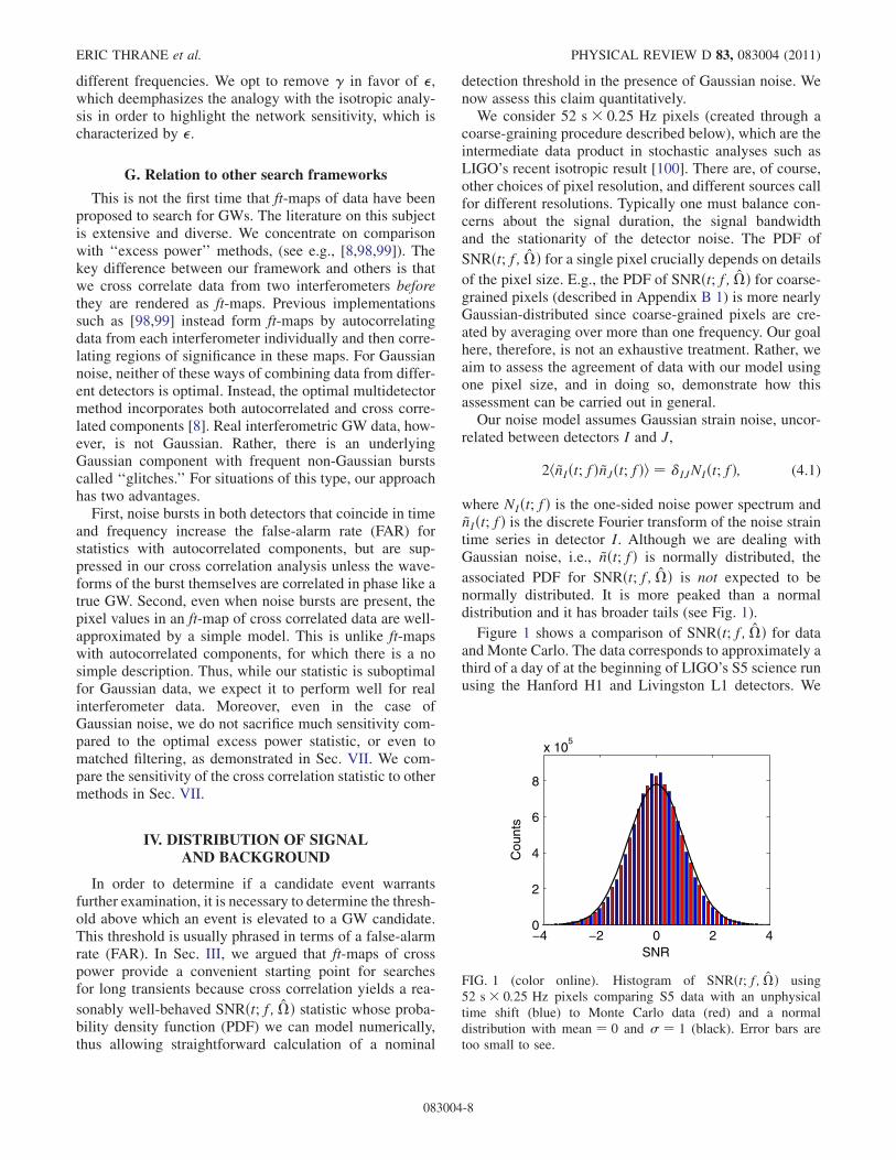
associated PDF for SNRðt; f; �Þ is not expected to benormally distributed. It is more peaked than a normaldistribution and it has broader tails (see Fig. 1).

Figure 1 shows a comparison of SNRðt; f; �Þ for dataand Monte Carlo. The data corresponds to approximately athird of a day of at the beginning of LIGO’s S5 science runusing the Hanford H1 and Livingston L1 detectors. We

−4 −2 0 2 40

2

4

6

8

x 105

SNR

Cou

nts

FIG. 1 (color online). Histogram of SNRðt; f; �Þ using52 s� 0:25 Hz pixels comparing S5 data with an unphysicaltime shift (blue) to Monte Carlo data (red) and a normaldistribution with mean ¼ 0 and � ¼ 1 (black). Error bars aretoo small to see.

ERIC THRANE et al. PHYSICAL REVIEW D 83, 083004 (2011)

083004-8

introduce an unphysical time shift between the two datastreams to remove all astrophysical content. Additional dataprocessing details are described in Appendix. B 1 and B 2,

as the precise shape of the PDF for SNRðt; f; �Þ dependscrucially on details of how time series data is processed.

The Monte Carlo histogram is scaled by a normaliza-tion factor (derived analytically in Appendix B 2), whichtakes into account data processing not included in ourMonte Carlo simulation, e.g., coarse-graining. After ap-plying this normalization factor, we find that the standarddeviation of the data and Monte Carlo distributions agreeto better than four significant digits. We conclude thatdata and Monte Carlo are in qualitative agreement. Thuswe expect that the data are well-behaved enough that wecan use a Gaussian noise model to assign a detectioncandidate threshold for SNR�, at least for this choice ofpixel size.

V. PATTERN RECOGNITION

In this section we showcase the cross power statisticdeveloped in Sec. III using two different implementations(the box-search and the Radon search) designed to addresstwo different type of astrophysical scenarios (broadbandsignals and narrow band signals).

A. Broadband box-search

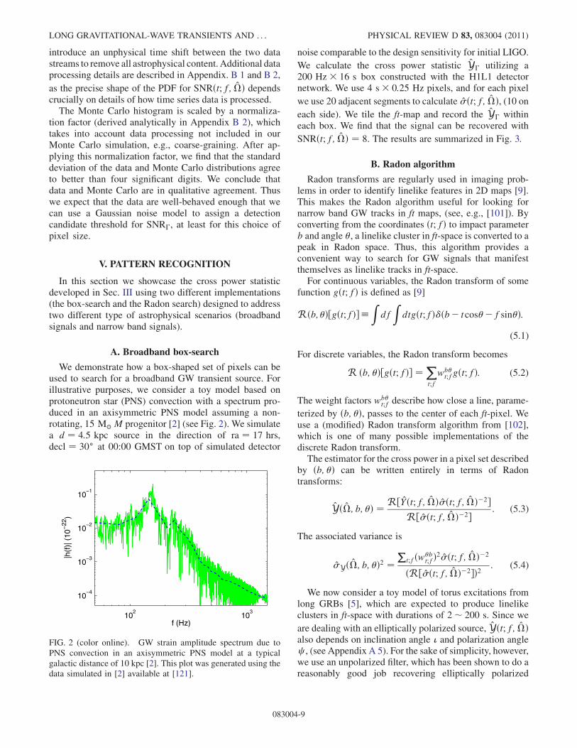
We demonstrate how a box-shaped set of pixels can beused to search for a broadband GW transient source. Forillustrative purposes, we consider a toy model based onprotoneutron star (PNS) convection with a spectrum pro-duced in an axisymmetric PNS model assuming a non-rotating, 15 M� M progenitor [2] (see Fig. 2). We simulatea d ¼ 4:5 kpc source in the direction of ra ¼ 17 hrs,decl ¼ 30� at 00:00 GMST on top of simulated detector

noise comparable to the design sensitivity for initial LIGO.

We calculate the cross power statistic Y� utilizing a200 Hz� 16 s box constructed with the H1L1 detectornetwork. We use 4 s� 0:25 Hz pixels, and for each pixel

we use 20 adjacent segments to calculate �ðt; f; �Þ, (10 oneach side). We tile the ft-map and record the Y� withineach box. We find that the signal can be recovered with

SNRðt; f; �Þ ¼ 8. The results are summarized in Fig. 3.

B. Radon algorithm

Radon transforms are regularly used in imaging prob-lems in order to identify linelike features in 2D maps [9].This makes the Radon algorithm useful for looking fornarrow band GW tracks in ft maps, (see, e.g., [101]). Byconverting from the coordinates ðt; fÞ to impact parameterb and angle , a linelike cluster in ft-space is converted to apeak in Radon space. Thus, this algorithm provides aconvenient way to search for GW signals that manifestthemselves as linelike tracks in ft-space.For continuous variables, the Radon transform of some

function gðt; fÞ is defined as [9]

Rðb;Þ½gðt;fÞ��Zdf

Zdtgðt;fÞ�ðb� tcos�f sinÞ:

(5.1)

For discrete variables, the Radon transform becomes

R ðb; Þ½gðt; fÞ� ¼ Xt;f

wbt;fgðt; fÞ: (5.2)

The weight factors wbt;f describe how close a line, parame-

terized by ðb; Þ, passes to the center of each ft-pixel. Weuse a (modified) Radon transform algorithm from [102],which is one of many possible implementations of thediscrete Radon transform.The estimator for the cross power in a pixel set described

by ðb; Þ can be written entirely in terms of Radontransforms:

Yð�; b; Þ ¼ R½Yðt; f; �Þ�ðt; f; �Þ�2�R½�ðt; f; �Þ�2� : (5.3)

The associated variance is

�Yð�; b; Þ2 ¼P

t;fðwbt;fÞ2�ðt; f; �Þ�2

ðR½�ðt; f; �Þ�2�Þ2 : (5.4)

We now consider a toy model of torus excitations fromlong GRBs [5], which are expected to produce linelikeclusters in ft-space with durations of 2� 200 s. Since we

are dealing with an elliptically polarized source, Yðt; f; �Þalso depends on inclination angle � and polarization anglec , (see Appendix A 5). For the sake of simplicity, however,we use an unpolarized filter, which has been shown to do areasonably good job recovering elliptically polarized

102

103

10−4

10−3

10−2

10−1

f (Hz)

|h(f

)| (

10−

22)

FIG. 2 (color online). GW strain amplitude spectrum due toPNS convection in an axisymmetric PNS model at a typicalgalactic distance of 10 kpc [2]. This plot was generated using thedata simulated in [2] available at [121].

LONG GRAVITATIONAL-WAVE TRANSIENTS AND . . . PHYSICAL REVIEW D 83, 083004 (2011)

083004-9

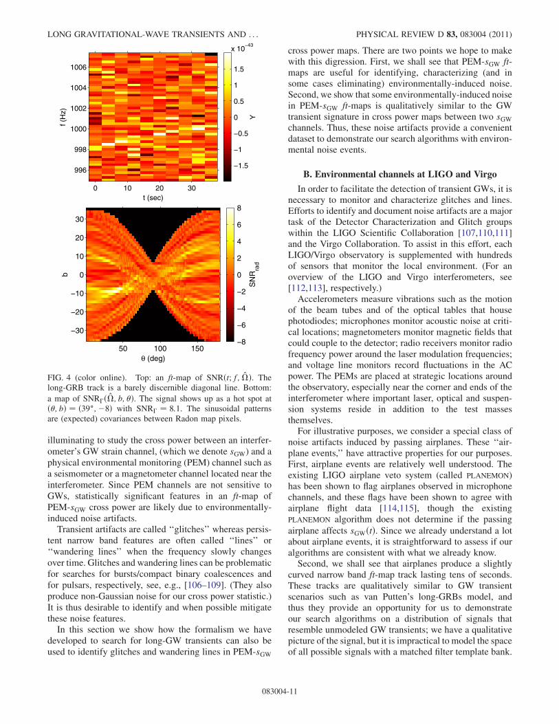
sources [103]. We simulate an elliptically polarized wave-form (see Table III) on top of simulated detector noisecomparable to design sensitivity for initial LIGO. Onceagain, we use 4 s� 0:25 Hz pixels, and for each pixel we

use 18 adjacent segments to calculate �ðt; f; �Þ (9 from

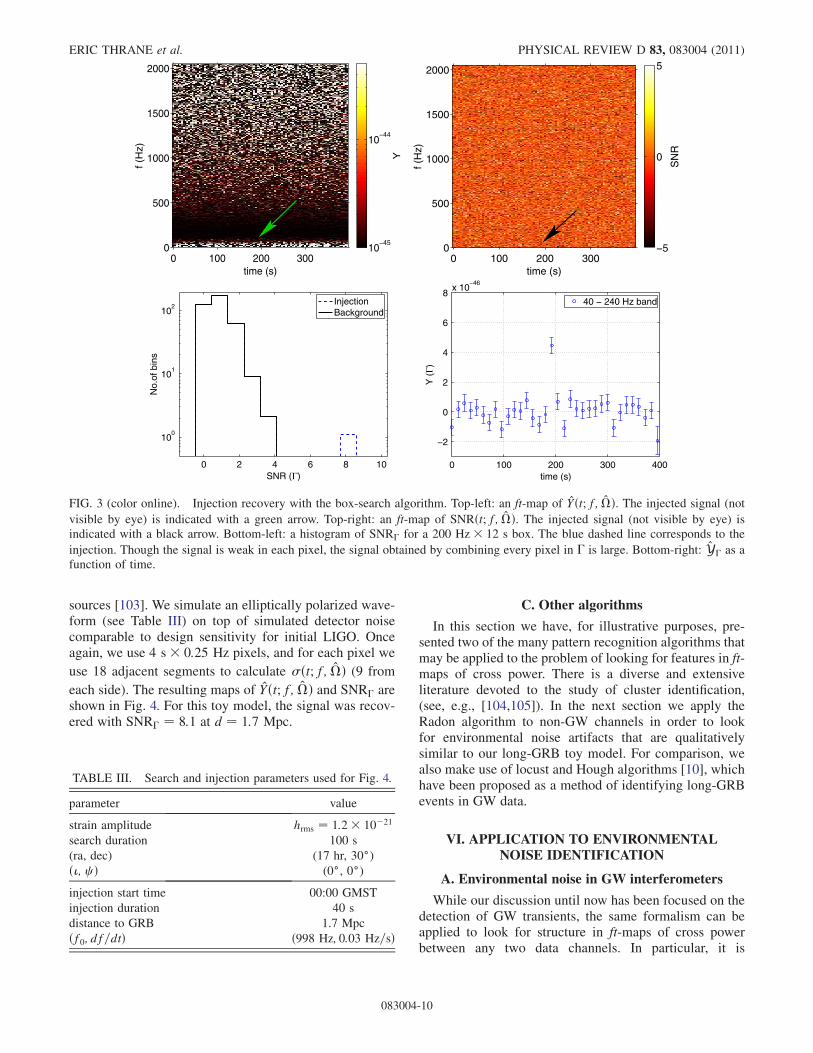
each side). The resulting maps of Yðt; f; �Þ and SNR� areshown in Fig. 4. For this toy model, the signal was recov-ered with SNR� ¼ 8:1 at d ¼ 1:7 Mpc.

C. Other algorithms

In this section we have, for illustrative purposes, pre-sented two of the many pattern recognition algorithms thatmay be applied to the problem of looking for features in ft-maps of cross power. There is a diverse and extensiveliterature devoted to the study of cluster identification,(see, e.g., [104,105]). In the next section we apply theRadon algorithm to non-GW channels in order to lookfor environmental noise artifacts that are qualitativelysimilar to our long-GRB toy model. For comparison, wealso make use of locust and Hough algorithms [10], whichhave been proposed as a method of identifying long-GRBevents in GW data.

VI. APPLICATION TO ENVIRONMENTALNOISE IDENTIFICATION

A. Environmental noise in GW interferometers

While our discussion until now has been focused on thedetection of GW transients, the same formalism can beapplied to look for structure in ft-maps of cross powerbetween any two data channels. In particular, it is

TABLE III. Search and injection parameters used for Fig. 4.

parameter value

strain amplitude hrms ¼ 1:2� 10�21

search duration 100 s

(ra, dec) (17 hr, 30�)ð�; c Þ (0�, 0�)

injection start time 00:00 GMST

injection duration 40 s

distance to GRB 1.7 Mpc

ðf0; df=dtÞ ð998 Hz; 0:03 Hz=sÞ

time (s)

f (H

z)

0 100 200 3000

500

1000

1500

2000

Y

10−45

10−44

time (s)

f (H

z)

0 100 200 3000

500

1000

1500

2000

SN

R

−5

0

5

0 2 4 6 8 10

100

101

102

SNR (Γ)

No.

of b

ins

InjectionBackground

0 100 200 300 400

−2

0

2

4

6

8x 10

−46

time (s)

Y (

Γ)

40 − 240 Hz band

FIG. 3 (color online). Injection recovery with the box-search algorithm. Top-left: an ft-map of Yðt; f; �Þ. The injected signal (not

visible by eye) is indicated with a green arrow. Top-right: an ft-map of SNRðt; f; �Þ. The injected signal (not visible by eye) isindicated with a black arrow. Bottom-left: a histogram of SNR� for a 200 Hz� 12 s box. The blue dashed line corresponds to the

injection. Though the signal is weak in each pixel, the signal obtained by combining every pixel in � is large. Bottom-right: Y� as afunction of time.

ERIC THRANE et al. PHYSICAL REVIEW D 83, 083004 (2011)

083004-10

illuminating to study the cross power between an interfer-ometer’s GW strain channel, (which we denote sGW) and aphysical environmental monitoring (PEM) channel such asa seismometer or a magnetometer channel located near theinterferometer. Since PEM channels are not sensitive toGWs, statistically significant features in an ft-map ofPEM-sGW cross power are likely due to environmentally-induced noise artifacts.

Transient artifacts are called ‘‘glitches’’ whereas persis-tent narrow band features are often called ‘‘lines’’ or‘‘wandering lines’’ when the frequency slowly changesover time. Glitches and wandering lines can be problematicfor searches for bursts/compact binary coalescences andfor pulsars, respectively, see, e.g., [106–109]. (They alsoproduce non-Gaussian noise for our cross power statistic.)It is thus desirable to identify and when possible mitigatethese noise features.

In this section we show how the formalism we havedeveloped to search for long-GW transients can also beused to identify glitches and wandering lines in PEM-sGW

cross power maps. There are two points we hope to makewith this digression. First, we shall see that PEM-sGW ft-maps are useful for identifying, characterizing (and insome cases eliminating) environmentally-induced noise.Second, we show that some environmentally-induced noisein PEM-sGW ft-maps is qualitatively similar to the GWtransient signature in cross power maps between two sGWchannels. Thus, these noise artifacts provide a convenientdataset to demonstrate our search algorithms with environ-mental noise events.

B. Environmental channels at LIGO and Virgo

In order to facilitate the detection of transient GWs, it isnecessary to monitor and characterize glitches and lines.Efforts to identify and document noise artifacts are a majortask of the Detector Characterization and Glitch groupswithin the LIGO Scientific Collaboration [107,110,111]and the Virgo Collaboration. To assist in this effort, eachLIGO/Virgo observatory is supplemented with hundredsof sensors that monitor the local environment. (For anoverview of the LIGO and Virgo interferometers, see[112,113], respectively.)Accelerometers measure vibrations such as the motion

of the beam tubes and of the optical tables that housephotodiodes; microphones monitor acoustic noise at criti-cal locations; magnetometers monitor magnetic fields thatcould couple to the detector; radio receivers monitor radiofrequency power around the laser modulation frequencies;and voltage line monitors record fluctuations in the ACpower. The PEMs are placed at strategic locations aroundthe observatory, especially near the corner and ends of theinterferometer where important laser, optical and suspen-sion systems reside in addition to the test massesthemselves.For illustrative purposes, we consider a special class of

noise artifacts induced by passing airplanes. These ‘‘air-plane events,’’ have attractive properties for our purposes.First, airplane events are relatively well understood. Theexisting LIGO airplane veto system (called PLANEMON)has been shown to flag airplanes observed in microphonechannels, and these flags have been shown to agree withairplane flight data [114,115], though the existingPLANEMON algorithm does not determine if the passing

airplane affects sGWðtÞ. Since we already understand a lotabout airplane events, it is straightforward to assess if ouralgorithms are consistent with what we already know.Second, we shall see that airplanes produce a slightly

curved narrow band ft-map track lasting tens of seconds.These tracks are qualitatively similar to GW transientscenarios such as van Putten’s long-GRBs model, andthus they provide an opportunity for us to demonstrateour search algorithms on a distribution of signals thatresemble unmodeled GW transients; we have a qualitativepicture of the signal, but it is impractical to model the spaceof all possible signals with a matched filter template bank.

t (sec)

f (H

z)

0 10 20 30

996

998

1000

1002

1004

1006

Y

−1.5

−1

−0.5

0

0.5

1

1.5

x 10−43

θ (deg)

b

50 100 150

−30

−20

−10

0

10

20

30

SN

Rra

d

−8

−6

−4

−2

0

2

4

6

8

FIG. 4 (color online). Top: an ft-map of SNRðt; f; �Þ. Thelong-GRB track is a barely discernible diagonal line. Bottom:

a map of SNR�ð�; b; Þ. The signal shows up as a hot spot atð; bÞ ¼ ð39�;�8Þ with SNR� ¼ 8:1. The sinusoidal patternsare (expected) covariances between Radon map pixels.

LONG GRAVITATIONAL-WAVE TRANSIENTS AND . . . PHYSICAL REVIEW D 83, 083004 (2011)

083004-11

C. Airplane noise identification

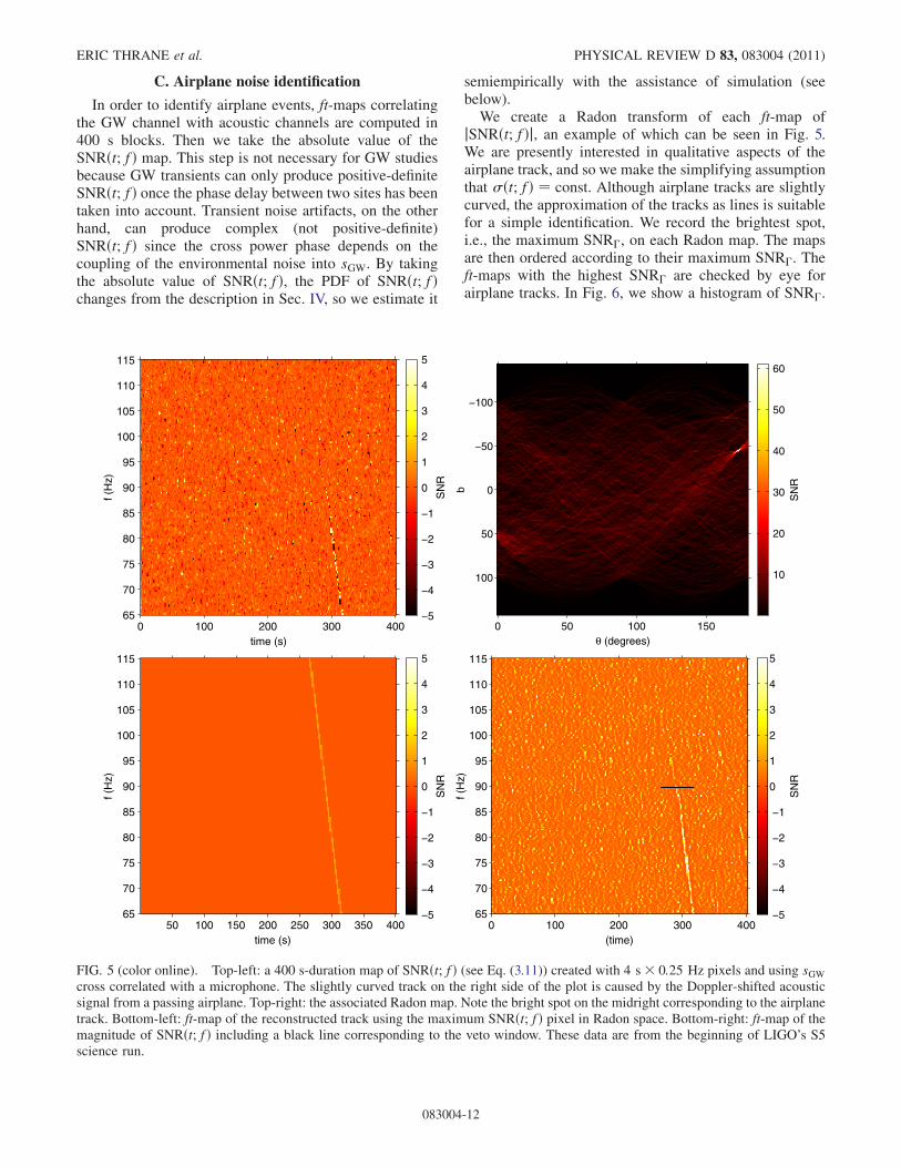
In order to identify airplane events, ft-maps correlatingthe GW channel with acoustic channels are computed in400 s blocks. Then we take the absolute value of theSNRðt; fÞ map. This step is not necessary for GW studiesbecause GW transients can only produce positive-definiteSNRðt; fÞ once the phase delay between two sites has beentaken into account. Transient noise artifacts, on the otherhand, can produce complex (not positive-definite)SNRðt; fÞ since the cross power phase depends on thecoupling of the environmental noise into sGW. By takingthe absolute value of SNRðt; fÞ, the PDF of SNRðt; fÞchanges from the description in Sec. IV, so we estimate it

semiempirically with the assistance of simulation (seebelow).We create a Radon transform of each ft-map of

jSNRðt; fÞj, an example of which can be seen in Fig. 5.We are presently interested in qualitative aspects of theairplane track, and so we make the simplifying assumptionthat �ðt; fÞ ¼ const. Although airplane tracks are slightlycurved, the approximation of the tracks as lines is suitablefor a simple identification. We record the brightest spot,i.e., the maximum SNR�, on each Radon map. The mapsare then ordered according to their maximum SNR�. Theft-maps with the highest SNR� are checked by eye forairplane tracks. In Fig. 6, we show a histogram of SNR�.

time (s)

f (H

z)

0 100 200 300 40065

70

75

80

85

90

95

100

105

110

115

SN

R

−5

−4

−3

−2

−1

0

1

2

3

4

5

θ (degrees)

b

0 50 100 150

−100

−50

0

50

100

SN

R

10

20

30

40

50

60

time (s)

f (H

z)

50 100 150 200 250 300 350 40065

70

75

80

85

90

95

100

105

110

115

SN

R

−5

−4

−3

−2

−1

0

1

2

3

4

5

(time)

f (H

z)

0 100 200 300 40065

70

75

80

85

90

95

100

105

110

115

SN

R

−5

−4

−3

−2

−1

0

1

2

3

4

5

FIG. 5 (color online). Top-left: a 400 s-duration map of SNRðt; fÞ (see Eq. (3.11)) created with 4 s� 0:25 Hz pixels and using sGWcross correlated with a microphone. The slightly curved track on the right side of the plot is caused by the Doppler-shifted acousticsignal from a passing airplane. Top-right: the associated Radon map. Note the bright spot on the midright corresponding to the airplanetrack. Bottom-left: ft-map of the reconstructed track using the maximum SNRðt; fÞ pixel in Radon space. Bottom-right: ft-map of themagnitude of SNRðt; fÞ including a black line corresponding to the veto window. These data are from the beginning of LIGO’s S5science run.

ERIC THRANE et al. PHYSICAL REVIEW D 83, 083004 (2011)

083004-12

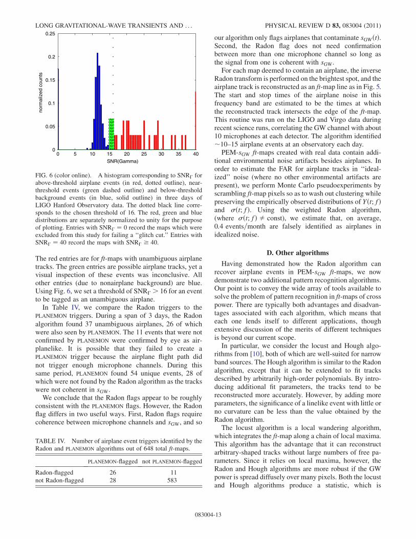
The red entries are for ft-maps with unambiguous airplanetracks. The green entries are possible airplane tracks, yet avisual inspection of these events was inconclusive. Allother entries (due to nonairplane background) are blue.Using Fig. 6, we set a threshold of SNR� > 16 for an eventto be tagged as an unambiguous airplane.

In Table IV, we compare the Radon triggers to thePLANEMON triggers. During a span of 3 days, the Radon

algorithm found 37 unambiguous airplanes, 26 of whichwere also seen by PLANEMON. The 11 events that were notconfirmed by PLANEMON were confirmed by eye as air-planelike. It is possible that they failed to create aPLANEMON trigger because the airplane flight path did

not trigger enough microphone channels. During thissame period, PLANEMON found 54 unique events, 28 ofwhich were not found by the Radon algorithm as the trackswere not coherent in sGW.

We conclude that the Radon flags appear to be roughlyconsistent with the PLANEMON flags. However, the Radonflag differs in two useful ways. First, Radon flags requirecoherence between microphone channels and sGW, and so

our algorithm only flags airplanes that contaminate sGWðtÞ.Second, the Radon flag does not need confirmationbetween more than one microphone channel so long asthe signal from one is coherent with sGW.For each map deemed to contain an airplane, the inverse

Radon transform is performed on the brightest spot, and theairplane track is reconstructed as an ft-map line as in Fig. 5.The start and stop times of the airplane noise in thisfrequency band are estimated to be the times at whichthe reconstructed track intersects the edge of the ft-map.This routine was run on the LIGO and Virgo data duringrecent science runs, correlating the GW channel with about10 microphones at each detector. The algorithm identified�10–15 airplane events at an observatory each day.PEM-sGW ft-maps created with real data contain addi-

tional environmental noise artifacts besides airplanes. Inorder to estimate the FAR for airplane tracks in ‘‘ideal-ized’’ noise (where no other environmental artifacts arepresent), we perform Monte Carlo pseudoexperiments byscrambling ft-map pixels so as to wash out clustering whilepreserving the empirically observed distributions of Yðt; fÞand �ðt; fÞ. Using the weighted Radon algorithm,(where �ðt; fÞ � const), we estimate that, on average,0:4 events=month are falsely identified as airplanes inidealized noise.

D. Other algorithms

Having demonstrated how the Radon algorithm canrecover airplane events in PEM-sGW ft-maps, we nowdemonstrate two additional pattern recognition algorithms.Our point is to convey the wide array of tools available tosolve the problem of pattern recognition in ft-maps of crosspower. There are typically both advantages and disadvan-tages associated with each algorithm, which means thateach one lends itself to different applications, thoughextensive discussion of the merits of different techniquesis beyond our current scope.In particular, we consider the locust and Hough algo-

rithms from [10], both of which are well-suited for narrowband sources. The Hough algorithm is similar to the Radonalgorithm, except that it can be extended to fit tracksdescribed by arbitrarily high-order polynomials. By intro-ducing additional fit parameters, the tracks tend to bereconstructed more accurately. However, by adding moreparameters, the significance of a linelike event with little orno curvature can be less than the value obtained by theRadon algorithm.The locust algorithm is a local wandering algorithm,

which integrates the ft-map along a chain of local maxima.This algorithm has the advantage that it can reconstructarbitrary-shaped tracks without large numbers of free pa-rameters. Since it relies on local maxima, however, theRadon and Hough algorithms are more robust if the GWpower is spread diffusely over many pixels. Both the locustand Hough algorithms produce a statistic, which is

0 5 10 15 20 25 30 35 400

0.05

0.1

0.15

0.2

0.25

SNR(Gamma)

norm

aliz

ed c

ount

s

FIG. 6 (color online). A histogram corresponding to SNR� forabove-threshold airplane events (in red, dotted outline), near-threshold events (green dashed outline) and below-thresholdbackground events (in blue, solid outline) in three days ofLIGO Hanford Observatory data. The dotted black line corre-sponds to the chosen threshold of 16. The red, green and bluedistributions are separately normalized to unity for the purposeof plotting. Entries with SNR� ¼ 0 record the maps which wereexcluded from this study for failing a ‘‘glitch cut.’’ Entries withSNR� ¼ 40 record the maps with SNR� � 40.

TABLE IV. Number of airplane event triggers identified by theRadon and PLANEMON algorithms out of 648 total ft-maps.

PLANEMON-flagged not PLANEMON-flagged

Radon-flagged 26 11

not Radon-flagged 28 583

LONG GRAVITATIONAL-WAVE TRANSIENTS AND . . . PHYSICAL REVIEW D 83, 083004 (2011)

083004-13

the integral of cross power along a track. We estimatesignificance by performing Monte Carlo pseudoexperi-ments in which we randomly scramble the ft-map pixels.

Applying the locust and Hough algorithms to an unam-biguous airplane event, we obtain the reconstruction plotsshown in Fig. 7. We determine that both the locust andHough algorithms detect the event with a FAR no morethan 0.04% per 400 s map in idealized noise.

VII. COMPARISON WITH OTHER TECHNIQUES

In this section, we compare the proposed excess crosspower statistic to matched filtering and to the generalexcess power statistic from [8]. It is impractical to actuallycarry out a matched filtering analysis since we do not havea template bank from which we can construct an arbitrarytransient signal. Nevertheless, it is possible to performanalytical estimates.

We consider a signal space characterized by anft-volume V spanned byNeff independent matched filteringtemplates. The ft-volume is simply the number of pixels inour pixel set �. We endeavor to address the following

question: given a false-alarm probability (FAP) and afalse-dismissal probability (FDP), what is the minimumsignal amplitude detectable by either method? Following[8], we, respectively, define thresholds ACP

min, AEPmin and A

MFmin

as the minimum detectable amplitudes by our cross power(CP) search, by the optimal total excess power (EP) search[8], (which includes both cross power and autopowerterms) and by a matched filter search (MF). The ratio ofthe corresponding amplitudes is (by definition) the effi-ciency of the excess power statistic compared to matchedfiltering:

�EPMFðFAP; FDP; Neff ; VÞ ¼ AMFmin=A

EPmin (7.1)

�CPEPðFAP; FDP; VÞ ¼ AEPmin=A

CPmin: (7.2)

To calculate these thresholds, signal and noise distribu-tions for CP and EP are generated using Monte Carlosimulations. Throughout this section we assume stationaryGaussian white noise; simulated signals are characterizedonly by their amplitude, polarization and ft-volume. Othercharacteristics such as frequency content, evolution withtime, etc. are not relevant for this white noise calculation.Following [8], we approximate the MF threshold as

AMFmin � AEP

minðFAP=Neff ; FDP; 1=2Þ: (7.3)

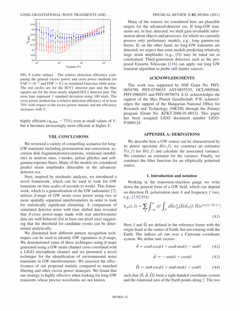
In Fig. 8, we plot �EPMF as a function of V andNeff . We seethat �EPMF * 50% over the range of parameter spaceconsidered.To compare the CP method to the EP method, we

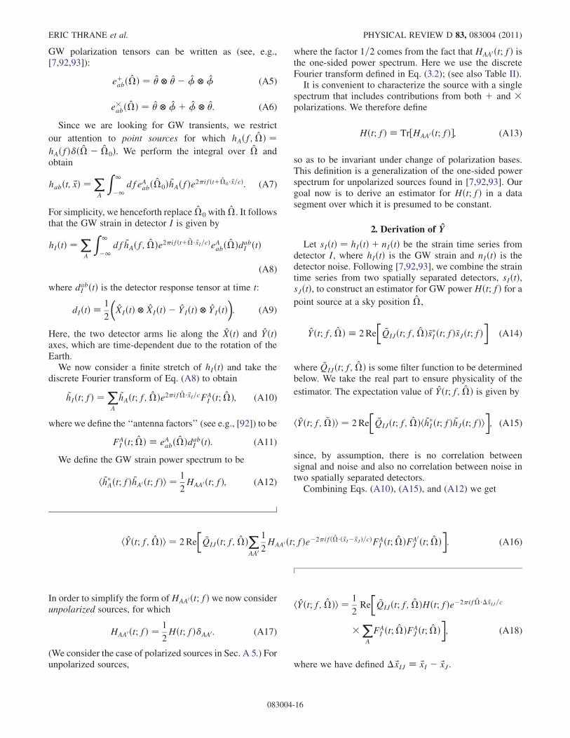
calculate �CPEP for the Hanford-Livingston and Hanford-Virgo networks averaging over an isotropically distributedpopulation of unpolarized GW sources. In Fig. 9 we plot�CPEP as a function of ft-volume V. The CP technique is

time (s)

f (s)

100 150 200 250 300

70

80

90

100

110

|SN

R|

3

6

9

12

15

18

time (s)

f (H

z)

100 150 200 250 300

70

80

90

100

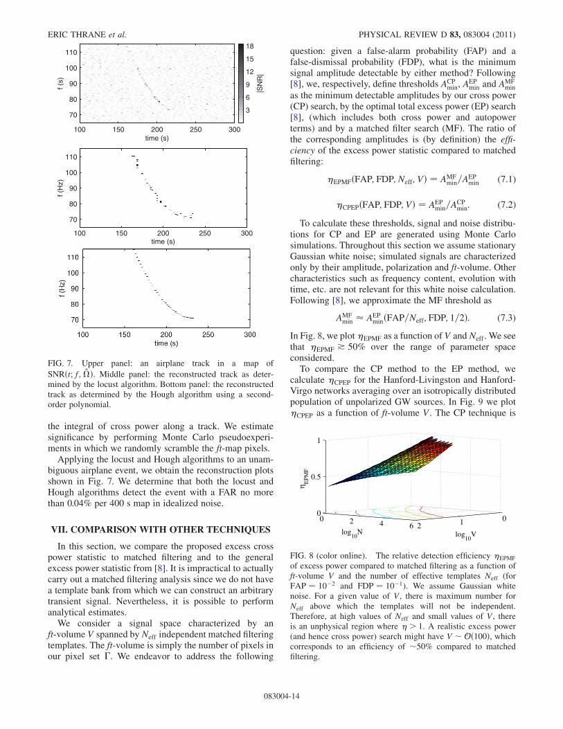
110

FIG. 7. Upper panel: an airplane track in a map of

SNRðt; f; �Þ. Middle panel: the reconstructed track as deter-mined by the locust algorithm. Bottom panel: the reconstructedtrack as determined by the Hough algorithm using a second-order polynomial.

0120 2 4 6

0

0.5

1

log10

Vlog10

N

η EPM

F

FIG. 8 (color online). The relative detection efficiency �EPMF

of excess power compared to matched filtering as a function offt-volume V and the number of effective templates Neff (forFAP ¼ 10�2 and FDP ¼ 10�1). We assume Gaussian whitenoise. For a given value of V, there is maximum number forNeff above which the templates will not be independent.Therefore, at high values of Neff and small values of V, thereis an unphysical region where �> 1. A realistic excess power(and hence cross power) search might have V �Oð100Þ, whichcorresponds to an efficiency of �50% compared to matchedfiltering.

ERIC THRANE et al. PHYSICAL REVIEW D 83, 083004 (2011)

083004-14

highly efficient (�CPEP � 77%) even at small values of V,but it becomes increasingly more efficient at higher V.

VIII. CONCLUSIONS

We reviewed a variety of compelling scenarios for long-GW transients including protoneutron star convection, ac-cretion disk fragmentation/excitations, rotational instabil-ities in neutron stars, r-modes, pulsar glitches and soft-gamma-repeater flares. Many of the models we consideredpredict strain amplitudes detectable in the advanced-detector era.

Next, inspired by stochastic analyses, we introduced anovel framework, which can be used to look for GWtransients on time scales of seconds to weeks. This frame-work, which is a generalization of the GW radiometer [7],utilizes ft-maps of GW strain cross power using two ormore spatially separated interferometers in order to lookfor statistically significant clustering. A comparison ofsimulated detector noise with time shifted data revealedthat ft-cross power-maps made with real interferometerdata are well-behaved (for at least one pixel size) suggest-ing that the threshold for candidate events can be deter-mined analytically.

We illustrated how different pattern recognition tech-niques can be used to identify GW signatures in ft-maps.We demonstrated some of these techniques using ft-mapsgenerated using a GW strain channel cross correlated witha LIGO microphone channel and we presented a noveltechnique for the identification of environmental noisetransients in GW interferometers. We assessed the effec-tiveness of our proposed statistic compared to matchedfiltering and other excess power strategies. We found thatour strategy is highly effective when looking for long-GWtransients whose precise waveforms are not known.

Many of the sources we considered here are plausibletargets for the advanced-detector era. If long-GW tran-sients are, in fact, detected, we shall gain invaluable infor-mation about objects and processes, for which we currentlypossess only preliminary models, e.g., long gamma-raybursts. If, on the other hand, no long-GW transients aredetected, we expect that some models predicting relativelylarge strain amplitudes (e.g., [5]) may be ruled out orconstrained. Third-generation detectors such as the pro-posed Einstein Telescope [116] can apply our long GWtransient algorithm to probe still fainter sources.

ACKNOWLEDGMENTS

This work was supported by NSF Grant No. PHY-0854790, PHY-0758035 AST-0855535, OCI-0905046,PHY-0960291 and PHY-0970074. S. G. acknowledges thesupport of the Max Planck Gesellschaft. P. R. acknowl-edges the support of the Hungarian National Office forResearch and Technology (NKTH) through the Polanyiprogram (Grant No. KFKT-2006-01-0012). This paperhas been assigned LIGO document number LIGO-P1000124.

APPENDIX A: DERIVATIONS

We describe how a GW source can be characterized byits power spectrum Hðt; fÞ, we construct an estimator

Yðt; fÞ for Hðt; fÞ and calculate the associated variance.We construct an estimator for the variance. Finally, weconstruct the filter function for an elliptically polarizedsource.

1. Introduction and notation

Working in the transverse-traceless gauge we writedown the general form of a GW field, which can depend

on direction �, polarization state A and frequency f (see,e.g., [7,92,93]):

habðt; ~xÞ ¼XA

Z 1

�1df

ZS2d�eAabð�Þ~hAðf; �Þe2�ifðtþ� ~x=cÞ:

(A1)

Here ~x and � are defined in the reference frame with theorigin fixed at the center of Earth, but not rotating with theEarth. The indices ab run over a Cartesian coordinatesystem. We define unit vectors

¼ cos cos xþ cos sin y� sinz (A2)

¼ � sin xþ cos y (A3)

� ¼ sin cos xþ sin sin yþ cosz (A4)

such that f; ; �g form a right-handed coordinate systemand the rotational axis of the Earth points along z. The two

101

102

103

104

0.6

0.65

0.7

0.75

0.8

0.85

0.9

0.95

1

Volume (V)

η CPE

P

FIG. 9 (color online). The relative detection efficiency com-paring the general excess power and cross power methods forFAP ¼ 10�2 and FDP ¼ 0:1 in simulated Gaussian white noise.The red circles are for the H1V1 detector pair and the bluesquares are for the more nearly aligned H1L1 detector pair. Theerror bars represent 1 standard deviation using 100 trials. Thecross power method has a relative detection efficiency of at least70% with respect to the excess power statistic and the efficiencyincreases with V.

LONG GRAVITATIONAL-WAVE TRANSIENTS AND . . . PHYSICAL REVIEW D 83, 083004 (2011)

083004-15

GW polarization tensors can be written as (see, e.g.,[7,92,93]):

eþabð�Þ ¼ � (A5)

e�abð�Þ ¼ þ : (A6)

Since we are looking for GW transients, we restrict

our attention to point sources for which hAðf; �Þ ¼hAðfÞ�ð�� �0Þ. We perform the integral over � andobtain

habðt; ~xÞ ¼XA

Z 1

�1dfeAabð�0Þ~hAðfÞe2�ifðtþ�0 ~x=cÞ: (A7)

For simplicity, we henceforth replace �0 with �. It followsthat the GW strain in detector I is given by

hIðtÞ ¼XA

Z 1

�1df~hAðf; �Þe2�ifðtþ� ~xI=cÞeAabð�ÞdabI ðtÞ

(A8)

where dabI ðtÞ is the detector response tensor at time t:

dIðtÞ � 1

2

�XIðtÞ XIðtÞ � YIðtÞ YIðtÞ

�: (A9)

Here, the two detector arms lie along the XðtÞ and YðtÞaxes, which are time-dependent due to the rotation of theEarth.

We now consider a finite stretch of hIðtÞ and take thediscrete Fourier transform of Eq. (A8) to obtain

~hIðt; fÞ ¼XA

~hAðt; f; �Þe2�if� ~xI=cFAI ðt; �Þ; (A10)

where we define the ‘‘antenna factors’’ (see e.g., [92]) to be

FAI ðt; �Þ � eAabð�ÞdabI ðtÞ: (A11)

We define the GW strain power spectrum to be

h~hAðt; fÞ~hA0 ðt; fÞi ¼ 1

2HAA0 ðt; fÞ; (A12)

where the factor 1=2 comes from the fact that HAA0 ðt; fÞ isthe one-sided power spectrum. Here we use the discreteFourier transform defined in Eq. (3.2); (see also Table II).It is convenient to characterize the source with a single

spectrum that includes contributions from both þ and �polarizations. We therefore define

Hðt; fÞ � Tr½HAA0 ðt; fÞ�; (A13)

so as to be invariant under change of polarization bases.This definition is a generalization of the one-sided powerspectrum for unpolarized sources found in [7,92,93]. Ourgoal now is to derive an estimator for Hðt; fÞ in a datasegment over which it is presumed to be constant.

2. Derivation of Y

Let sIðtÞ ¼ hIðtÞ þ nIðtÞ be the strain time series fromdetector I, where hIðtÞ is the GW strain and nIðtÞ is thedetector noise. Following [7,92,93], we combine the straintime series from two spatially separated detectors, sIðtÞ,sJðtÞ, to construct an estimator for GW power Hðt; fÞ for apoint source at a sky position �,

Yðt; f; �Þ � 2Re

�~QIJðt; f; �Þ~sI ðt; fÞ~sJðt; fÞ

�(A14)

where ~QIJðt; f; �Þ is some filter function to be determinedbelow. We take the real part to ensure physicality of the

estimator. The expectation value of Yðt; f; �Þ is given by

hYðt; f; ~�Þi ¼ 2Re

�~QIJðt; f; �Þh~hI ðt; fÞ~hJðt; fÞi

�; (A15)

since, by assumption, there is no correlation betweensignal and noise and also no correlation between noise intwo spatially separated detectors.Combining Eqs. (A10), (A15), and (A12) we get

hYðt; f; �Þi ¼ 2Re

�~QIJðt; f; �ÞX

AA0

1

2HAA0 ðt; fÞe�2�ifð�ð ~xI� ~xJÞ=cÞFA

I ðt; �ÞFA0J ðt; �Þ

�: (A16)

In order to simplify the form ofHAA0 ðt; fÞ we now considerunpolarized sources, for which

HAA0 ðt; fÞ ¼ 1

2Hðt; fÞ�AA0 : (A17)

(We consider the case of polarized sources in Sec. A 5.) Forunpolarized sources,

hYðt; f; �Þi ¼ 1

2Re

�~QIJðt; f; �ÞHðt; fÞe�2�if�� ~xIJ=c

�XA

FAI ðt; �ÞFA

J ðt; �Þ�; (A18)

where we have defined � ~xIJ � ~xI � ~xJ.

ERIC THRANE et al. PHYSICAL REVIEW D 83, 083004 (2011)

083004-16

We desire that hYi ¼ Hðt; fÞ, which implies

~Q IJðt; f; �Þ ¼ 2e2�if�� ~xIJ=cPA F

AI ðt; �ÞFA

J ðt; �Þ : (A19)

By setting QIJðt; f; �Þ thusly, we account for the phasedifference between detectors I and J ensuring that thebracketed quantity in Eq. (A18) is real. We also accountfor the detector pair efficiency.

Finally, we define (unpolarized) pair efficiency as

�IJðt; �Þ � 1

2

XA

FAI ðt; �ÞFA

J ðt; �Þ; (A20)

which enables us to rewrite the filter function as

~Q IJðt; f; �Þ ¼ 1

�IJðt; �Þ e2�if�� ~xIJ=c: (A21)

Since Yðt; f; �Þ / ~Qðt; f; �Þ and ~Q / 1=�IJðt; f; �Þ, itfollows that Yðt; f; �Þ / 1=�IJðt; �Þ. This can be under-stood as follows. If we observe a modest value of strainpower from a direction associated with low efficiency, wemay infer (if the signal is statistically significant) that thetrue source power is much higher because the network only‘‘sees’’ some fraction of the true GW power.

3. Variance of the estimator

We derive an expression for the variance of Yðt; f; �Þ,�Yðt; f; �Þ2 � hYðt; f; �Þ2i � hYðt; f; �Þi2. In searchesfor persistent stochastic GWs, the second term is usuallyomitted and the first term is simplified by assuming thatsignal in each pixel is small compared to the noise. Suchsmall signals are extracted by averaging over a very largenumber of segments (see, e.g., [92]). Since we are dealingwith transients, however, the signal may be comparable tothe noise and so we can not neglect any terms in ourcalculation of �2

Y .To begin we define a new (complex-valued) estimator

that will be handy in our derivation of �2Y:

Wðt; f; �Þ � 2 ~QIJðt; f; �Þ~s?I ðt; fÞ~sJðt; fÞ: (A22)

Our GW power estimator Yðt; f; �Þ is simply the real part

of Wðt; f; �Þ:

Yðt; f; �Þ ¼ 1

2ðWðt; f; �Þ þ Wðt; f; �Þ?Þ: (A23)

For notational compactness, we shall omit the arguments

of Wðt; f; �Þ in the remainder of this derivation. It follows

that the variance of Yðt; f; �Þ can be written as

�2Y ¼ 1

4½ðhW2i � hWi2Þ þ ðhW?2i � hW?i2Þ þ 2�2

W�;(A24)

where

�2W � hjWj2i � jhWij2: (A25)

Now we evaluate the three terms in Eq. (A24) beginningwith �2

W . We obtain

�2Wðt; f; �Þ ¼ 4

�h~sI ðt; fÞ~sJðt; fÞ~sIðt; fÞ~sJðt; fÞi

� h~sI ðt; fÞ~sJðt; fÞih~sIðt; fÞ~sJðt; fÞi�

��������� ~QIJðt; f; �Þ

��������2

: (A26)

For mean-zero Gaussian random variables, we can expandthe four-point correlation into a sum of products of two-point correlations. We substitute s ¼ hþ n and set signal-noise cross terms to zero along with noise-noise crossterms from different detectors. The variance becomes

�2Wðt; f; �Þ ¼ 4½h~hI ðt; fÞ~hIðt; fÞih~hJðt; fÞ~hJðt; fÞi

þ h~hI ðt; fÞ~hIðt; fÞih~nJðt; fÞ~nJðt; fÞiþ h~hJðt; fÞ~hJðt; fÞih~nI ðt; fÞ~nIðt; fÞiþ h~nI ðt; fÞ~nIðt; fÞih~nJðt; fÞ~nJðt; fÞi�� j ~QIJðt; f; �Þj2: (A27)

Evaluating the four terms in Eq. (A27), we obtain

�2Wðt;f;�Þ¼½�IIðt;�Þ�JJðt;�ÞHðt;fÞ2

þHðt;fÞð�IIðt;�ÞNJðt;fÞþ�JJðt;�ÞNIðt;fÞÞþNIðt;f;ÞNJðt;fÞ�j ~QIJðt;f;�Þj2; (A28)

where � is defined in Eq. (A20) and where NIðt; fÞ is theone-sided noise power spectra:

NIðt; fÞ � 2j~nIðt; fÞj2: (A29)

Using the same line of reasoning, we calculate theremaining terms in Eq. (A24):

hW2i � hWi2 ¼ hW?2i � hW?i2 ¼ Hðt; fÞ2: (A30)

Combining Eqs. (A24) and (A30), we conclude that

�2Y ¼ 1

2½�2

W þHðt; fÞ2�: (A31)

The factor of 1=2 comes about from the fact that Yðt; f; �Þis real whereas Wðt; f; �Þ is complex. We note that in thesmall-signal limit HðfÞ ! 0 and the variance reduces tothe canonical stochastic result [92]:

�2Y ! 1

2

�NIðt; fÞNJðt; fÞj ~QIJðt; f; �Þj2

�: (A32)

LONG GRAVITATIONAL-WAVE TRANSIENTS AND . . . PHYSICAL REVIEW D 83, 083004 (2011)

083004-17

4. Expectation value of �2Y

Our estimator for the variance of Y is given by

� 2Yðt; f; �Þ ¼ 1

2

�������� ~QIJðt; f; �Þ��������2

PadjI ðfÞPadj

J ðfÞ; (A33)

where PI is the average autopower in neighboring pixels:

PadjI ðfÞ � 2j~sIðfÞj2: (A34)

The overline denotes an average over neighboring pixels.By averaging over neighboring pixels, we assume that thedetector noise in any given pixel can be characterized bylooking at its neighbors. This assumption is discussedbelow.

Now we calculate the expectation value of our estimatorfor variance �2

Y given in Eq. (A33) in order to compare it tothe theoretical variance given in Eqs. (A31) and (A28).Equations (3.9) and (3.10) together imply

h�2Yðt;f;�Þi¼2j ~QIJðt;f;�Þj2hsadjI ðfÞsadjI ðfÞsadjJ ðfÞsadjJ ðfÞi:

(A35)

Using Eq. (A26) to write the expectation value of �2Y in

terms of the theoretical value of �2W , we find

h�2Yðt; f; �Þi ¼ 1

2

��2

Wðt; f; �Þ þ 4

�������� ~QIJðt; f; �Þ��������2

� h~sadjI ðt; fÞ~sadjJ ðt; fÞih~sadjI ðt; fÞ~sadjJ ðt; fÞi�

¼ 1

2

��2

Wðt; f; �Þ þ jhWij2�

¼ 1

2½�2

Wðt; f; �Þ þHðt; fÞ2�: (A36)

Since this is the theoretical variance from (A31), we con-clude that h�2

Yi ¼ �2Y . Thus, Eq. (3.9) provides an unbiased

estimator for �2Y . Here we have assumed that the noise and

signal are comparable in neighboring segments. This as-sumption can fail for rapidly changing, high-SNR signalsand also for highly nonstationary noise, and so additionalwork may be required to estimate � in these situations.

5. Elliptically polarized sources

A variety of long-transient GW sources are expected tobe elliptically polarized (e.g., long GRBs [4,5] and pulsarglitches [117]). Elliptically polarized sources are parame-terized by two angles. The inclination angle � is the anglebetween the rotational axis of the source and the observer’sline of sight and the polarization angle c describes theorientation of the rotational axis in the plane perpendicularto the line of sight (see, e.g., [118]).

Following [119], we characterize an elliptically polar-ized source with the so-called canonical amplitudes:

A� �

Aþ cos2c

Aþ sin2c

�A� sin2c

A� cos2c ;

0BBBBB@

1CCCCCA (A37)

where

Aþ � ðh0=2Þð1þ cos2�Þ (A38)

A� � h0 cos�: (A39)

We have set the initial phase 0 ¼ 0 for the sake ofsimplicity. (Ultimately, we are concerned with the averagecross power over many cycles and so the initial phase isunimportant.) Here h0 is the strain amplitude.Next, we define the tensor [119]

h�abðtÞ �

eþab cos½ ðtÞ�e�ab cos½ ðtÞ�eþab sin½ ðtÞ�e�ab sin½ ðtÞ�

0BBBBB@

1CCCCCA; (A40)

where ðtÞ describes the phase evolution of the signal[120]. Now we write the GW equation as [119]

habðtÞ�X�

A�h�abðtÞ

¼ðAþcosð2c Þcos½ ðtÞ��A� sinð2c Þsin½ ðtÞ�ÞeþabþðAþ sinð2c Þcos½ ðtÞ�þA�cosð2c Þsin½ ðtÞ�Þe�ab:

(A41)

We Fourier transform a finite stretch of GW signal to

obtain the coefficients ~hAðfÞ (see Eq. (A1)):

~hþðt; fÞ ¼½Aþ cosð2c Þ þ iA� sinð2c Þ��ff0

2Ns

(A42)

~h�ðt; fÞ ¼½Aþ sinð2c Þ � iA� cosð2c Þ��ff0

2Ns

: (A43)

We have ignored negative frequencies, which will play nopart in our subsequent calculation of one-sided GW power.Also, we have expanded ðtÞ in a Taylor series,

ðtÞ ¼ 0 þ 2�

�f0tþ 1

2_ft2�þOðt3Þ: (A44)

We assume that _f is approximately zero over the segmentduration, T. In principle, this formulation could be ex-tended to broadband sources, but we expect ellipticallypolarized sources (associated with spinning objects and abinary objects) to be narrow band.Combining Eqs. (A12) and (A42), we calculate the one-

sided power spectrum:

ERIC THRANE et al. PHYSICAL REVIEW D 83, 083004 (2011)

083004-18

HAA0 ðt; fÞ ¼ �ff0

2N2s

�A2þ cosð2c Þ2 þ A2� sinð2c Þ2 ðA2þ � A2�Þ cosð2c Þ sinð2c ÞðA2þ � A2�Þ cosð2c Þ sinð2c Þ A2þ sinð2c Þ2 þ A2� cosð2c Þ2

� �þ i

0 �AþA�AþA� 0

� ��: (A45)

The imaginary off-diagonal terms correspond to the phasedelay between þ and � polarization states.

Combining Eqs. (A13) and (A45), we obtain

Hðt; fÞ ¼ 1

2N2s

ðA2þ þ A2�Þ�ff0 : (A46)

Our goal, once again, is to find an estimator forHðt; fÞ. Weassume that the estimator for Hðt; fÞ can be constructed

from the cross power spectrum of two GW strainchannels multiplied by an appropriate filter function,~QIJðt; f; �; �; c Þ:Yðt; f; �; �; c Þ ¼ 2Re½~s?I ðt; fÞ~sJðt; fÞ ~QIJðt; f; �; �; c Þ�:

(A47)

Plugging Eq. (A45) and (A16), we obtain

hYðt; f; �; �; c Þi ¼ 2Re

�1

2

�ff0

2N2s

ðFþI F

þJ ½A2þ cosð2c Þ2 þ A2� sinð2c Þ2� þ Fþ

I F�J ½ðA2þ � A2�Þ cosð2c Þ sinð2c Þ � iAþA��

þ F�I F

þJ ½ðA2þ � A2�Þ cosð2c Þ sinð2c Þ þ iAþA��

þ F�I F

�J ½A2þ sinð2c Þ2 þ A2� cosð2c Þ2�Þe�2�ifð�� ~xIJ=cÞ ~QIJðt; f; �; �; c Þ

�: (A48)

We write the polarized filter function as

~Q IJðt; f; �; �; c Þ ¼ e2�if�� ~xIJ=cþi�=�ð�; �; c Þ; (A49)

where � is an angle arising from the phase delaybetween þ and � polarizations. By requiring that

hYðt;f;�;�;c Þi¼Hðt;fÞ, it follows that

�ð�;�;c Þ¼��������Fþ

I FþJ ½a2þcosð2c Þ2þa2� sinð2c Þ2�

þðFþI F

�J þF�

I FþJ Þða2þ�a2�Þcosð2c Þsinð2c Þ

þF�I F

�J ða2þ sinð2c Þ2þa2�cosð2c Þ2Þ

þ iaþa�ðF�I F

þJ �Fþ

I F�J Þ��������=ða2þþa2�Þ;

(A50)

and

�ð�;�;c Þ¼�phaseð½FþI F

þJ ½a2þcosð2c Þ2þa2� sinð2c Þ2�

þðFþI F

�J þF�

I FþJ Þða2þ�a2�Þcosð2c Þsinð2c Þ

þF�I F

�J ða2þ sinð2c Þ2þa2�cosð2c Þ2Þ

þ iaþa�ðF�I F

þJ �Fþ

I F�J Þ�=ða2þþa2�ÞÞ;

(A51)

where we have defined

aþ � Aþ=h0 (A52)

a� � A�=h0: (A53)

As a sanity check, we note that an elliptically polari-zed source with pure þ-polarization yields a sensibleefficiency

�ð�; � ¼ 90�; c ¼ 0Þ ¼ FþI F

þJ : (A54)

APPENDIX B: DATA PROCESSING DETAILS

1. Overview

In this we describe the detailed procedure for the crea-tion of the 52 s� 0:25 Hz coarse-grained data in Fig. 1.(i) Since nðtÞ is drawn from a zero-mean, unit-variance

normal distribution, the frequency domain data willbe zero-mean with a standard deviation scaled byffiffiffiffiffiffiffiffiffiN=2

pfor the real and imaginary parts separately

where N is the number of sampling points.(ii) To calculate the cross-spectral density, CSD, data

are first Hann windowed and zero padded in thetime domain. Discrete Fourier transforms are multi-plied to form cross power, then summed (with awindow that tapers at the ends) to yield a CSDwith 0.25 Hz resolution.

(iii) To calculate each PIðfÞ, data are broken into 4 sblocks with 50% overlap. Each block is Hannwindowed, and the resulting power samples fromall blocks are summed so that PIðfÞ also has0.25 Hz resolution.

(iv) Hann windowing reduces the overall power by afactor of 3=8. To compensate both the CSD andPIðfÞ are corrected for this factor.

(v) Without windowing or overlap each power estimatefrom each data block will be �2-distributed with 2degrees of freedom and scaled by N=2, and so theaverage of M blocks are �2-distributed with 2Mdegrees of freedom and scaled by N=2M.

(vi) Overlap changes the effective number of degrees offreedom in a way that can be calculated numeri-cally (see Appendix B 2).

LONG GRAVITATIONAL-WAVE TRANSIENTS AND . . . PHYSICAL REVIEW D 83, 083004 (2011)

083004-19

(vii) Without windowing, each cross power product willhave zero-mean and a standard deviation scaled by

N=ffiffiffi2

p. Summing M values gives each CSD esti-

mate a standard deviation scaled by NffiffiffiffiffiffiffiffiffiffiM=2

p.

(viii) These scaling behaviors indicate how we couldexpect SNR to behave, except for the nontrivialeffects of windowing, zero-padding and weightedaveraging. These somewhat subtle effects areevaluated explicitly in Appendix B 2.

2. Calculation of the normalization factor

Here we derive the stretch factor applied to the signal tonoise ratio (SNR) histogram in Fig. 1 generated usingsimulated Gaussian noise. Let fxng and fymg be real, dis-crete, time sequences corresponding to two independentdata streams with each xn and ym sampled from a(0, 1)-Gaussian distribution. The time domain fxng andfymg can be transformed into frequency domain sequencesof N complex numbers fXpg and fYqg using the discrete

Fourier transform (DFT), defined here as

Xp ¼ �tXN�1

n¼0

exp

��2�ipn

N

�xn and

Yq ¼ �tXN�1

m¼0

exp

��2�iqm

N

�ym: (B1)

The inverse DFT can be used to express the originaldiscrete-time signal as

xn ¼ �fXN�1

p¼0

exp

�2�ipn

N

�Xp and

ym ¼ �fXN�1

q¼0

exp

�2�iqm

N

�Yq: (B2)

To see the effects of zero-padding, we define the real,2N-periodic discrete-time signal ~x � fxn; 0ng where 0n is asequence of N-many zeros. Then

~X p ¼ �tX2N�1

n¼0

exp

��2�ipn

2N

�~xn

¼ �tXN�1

n¼0

exp

��2�ipn

2N

�xn (B3)

where

~xn ¼

8>>><>>>:xn ¼ �f

2

P2N�1p¼0 exp

�2�ipn2N

�~Xp

0n ¼ �f2

P2N�1p¼0 ð�1Þp exp

�2�ipn2N

�~Xp

(B4)

with 0 � n � N � 1.From Eq. (B4) we conclude that the Xp with 0 � p �

2N � 1 are not linearly independent. However, the X2p

(0 � p � N � 1) and X2pþ1 (0 � p � N � 1) are

separately linearly independent. In the calculations below,we use only the even terms to express both the even andodd Xk terms. Therefore, taking into account the zero-padding, we can write

xn ¼ �fXN�1

p¼0

exp

�2�ið2pÞn

2N

�~X2p

¼ �fXN�1

p¼0

exp

�2�ipn

N

�~X2p: (B5)

By comparing xn in Eqs. (B2) and (B5) we see that

~X 2p ¼ Xp: (B6)

In addition to the zero-padding, the windowing effect canbe expressed by defining ~u � fun; 0ng � fxnfðnÞ; 0ng withthe discrete Fourier transform given by

Uk ¼ �tX2N�1

n¼0

exp

��2�ikn

2N

�~un

¼ �tXN�1

n¼0

exp

��2�ikn

2N

�un

¼ �tXN�1

n¼0

exp

��2�ikn

2N

�fðnÞxn (B7)

where xn is given by Eq. (B5) and fðnÞ is the Hann windowdefined by

fðnÞ � 1

2

�1� cos

�2�n

N

��¼ X1

a¼�1

1

2

��1

2

�jajexp

�2�ina

N

�(B8)

with 0 � n � N � 1.After some algebra Eqs. (B5)–(B8) give

Uk ¼ �f�t

2

XN�1

n¼0

XN�1

p¼0

X1a¼�1

Xp

� exp

��2�inðk=2� p� aÞN

��� 1

2

�jaj: (B9)

Similarly, we can express the second data stream by ~v �fvm; 0mg � fymfðmÞ; 0mgwith 0 � m � N � 1. In analogywith (B9) the discrete Fourier transform is given by

Vk ¼ �f�t

2

XN�1

m¼0

XN�1

q¼0

X1b¼�1

Yq

� exp

��2�imðk=2� q� bÞN

��� 1

2

�jbj: (B10)

The sequences f~ung and f~vng are the real, 2N-periodic,discrete-time signals that are used in the code for thecalculation of the contribution of the (CSD) to the (SNR).

ERIC THRANE et al. PHYSICAL REVIEW D 83, 083004 (2011)

083004-20

From the definition

SNRðt;fÞ¼Re

�������� CSDxyðt;fÞffiffiffiffiffiffiffiffiffiffiffiffiffiffiffiffiffiffiffiffiffiffiffiffiffiffiffiffiffiffiffiffiffiffiffiffiffiffiffiffiffiffiPSDxðt;fÞPSDyðt;fÞ

q phaseðQðt;f;�ÞÞ��������;

(B11)

where Qðt; f; �Þ is the filter function, we observe that inorder to explain the SNR distribution obtained from theprocessed data we need to understand the statistical con-sequences of the code that calculates the power spectraldensity PSDx (or PSDy) and the CSDxy.

Since the CSD is the Fourier transform of the cross-covariance function, in order to characterize the numeratorof SNR we need to study terms of the form X

kYk. Without

windowing and without zero-padding the XkYk term de-

pends only on the frequency k as the following result shows(obtained using Eqs. (B1) and (B2)):

XkYk ¼

XN�1

n¼0

XN�1

m¼0

XN�1

p¼0

XN�1

q¼0

XpYq exp

�2�inðk� pÞ

N

�

� exp

��2�imðk� qÞN

�

¼ XN�1

p¼0

XN�1

q¼0

�pk�qkXpYq: (B12)

However, when we take into account the effects of win-dowing and zero-padding, the U

kVk term, contrary to the

XkYk term, has contributions from a wider part of the

frequency domain according to the following result:

UkVk ¼ 1

4

XN�1

n¼0

XN�1

m¼0

XN�1

p¼0

XN�1

q¼0

X1a¼�1

X1b¼�1

XpYq

�� 1

2

�jajþjbj

� exp

�2�inðk=2� p� aÞ

N

�

� exp

��2�imðk=2� q� bÞN

�: (B13)

To imitate the way the code is calculating the CSD, wedefine

Zj �Xþ13

k¼�13

wðkÞUjþkVjþk (B14)

where

wðkÞ ��1

2; 1; 1; . . . ; 1;|fflfflfflfflfflffl{zfflfflfflfflfflffl}

25-times

1

2

�: (B15)

It is easy to see that the expectation value of Zj is zero,

since the Xq and Yq are statistically independent with mean

zero. To evaluate the standard deviation of Zj=ffiffiffiffiffiffi26

p, where

the 26 is a normalization constant due to averaging, we

then need to evaluate hffiffiffiffiffiffiffiffiffiffiffiffiffiffiffiffiffiffiZjZj=26

qi (where there is no sum

over j). After some calculations, the final expression forhZ

jZji becomes

hZjZji ¼

Xk;k0;�;�0;�;�0

wðkÞwðk0Þ�ð�;�0Þ�ð�;�0Þ�1

4

�2

��� 1

2

�ðjajþjbjþja0jþjb0jÞ(B16)

where

�ð�;�0Þ � sin½ð�=2Þðk� k0 þ 2�� 2�0Þ�sin½ð�=2NÞðk� k0 þ 2�� 2�0Þ�� exp

��i�ð�� �0Þ

�1� 1

N

��: (B17)

Using N ¼ 212; 992, corresponding to 52 s of datasampled at 4, 096 Hz, the numerical result turned out to beffiffiffiffiffiffiffiffiffiffiffiffiffiffiffiffiffiffiffiffi

1

26hZ

jZjis

¼ 0:7208: (B18)

Multiplying this by the normalization factor of 8=3 due toHann window we get 1.922—the normalization factorapplied to MC in Fig. 1.

[1] J. Abadie et al. (The LIGO Scientific Collaboration),Phys. Rev. D 81, 102001 (2010).

[2] C. D. Ott, Classical Quantum Gravity 26, 063001 (2009).[3] A. Corsi and P. Meszaros, Astrophys. J. 702, 1171

(2009).[4] A. L. Piro and E. Pfahl, Astrophys. J. 658, 1173 (2007).[5] M. van Putten, Astrophys. J. Lett. 575, L71 (2002).[6] R. Prix, S. Giampanis, and C. Messenger, ‘‘Search Method

for Long-Duration Gravitational-Wave Transients fromNeutron Stars’’ (unpublished).

[7] B. Abbott et al. (LIGO Scientific Collaboration), Phys.Rev. D 76, 082003 (2007).

[8] W.G. Anderson, P. R. Brady, J. D. E. Creighton, and E. E.Flanagan, Phys. Rev. D 63, 042003 (2001).

[9] S. R. Deans, The Radon Transform and Some of itsApplications (Dover Publications, Inc., New York,2007), 2nd ed.

[10] P. Raffai et al., Classical Quantum Gravity 24, S457(2007).

[11] S. E. Woosley and J. S. Bloom, Annu. Rev. Astron.Astrophys. 44, 507 (2006).

[12] H.-T. Janka, K. Langanke, A. Marek, G. Martınez-Pinedo,and B. Muller, Phys. Rep. 442, 38 (2007).

[13] C. D. Ott, Classical Quantum Gravity 26, 204015 (2009).

LONG GRAVITATIONAL-WAVE TRANSIENTS AND . . . PHYSICAL REVIEW D 83, 083004 (2011)

083004-21

[14] H. Dimmelmeier, C. D. Ott, A. Marek, and H.-T. Janka,Phys. Rev. D 78, 064056 (2008).

[15] L. Dessart, A. Burrows, E. Livne, and C.D. Ott,Astrophys. J. 645, 534 (2006).

[16] E. Muller et al., Astrophys. J. 603, 221 (2004).[17] J.W. Murphy, C. D. Ott, and A. Burrows, Astrophys. J.

707, 1173 (2009).[18] A. Marek, H.-T. Janka, and E. Muller, Astron. Astrophys.

496, 475 (2009).[19] K. Kotake, W. Iwakami, N. Ohnishi, and S. Yamada,

Astrophys. J. Lett. 697, L133 (2009).[20] C. D. Ott, A. Burrows, L. Dessart, and E. Livne, Phys. Rev.

Lett. 96, 201102 (2006).[21] C. D. Ott, H. Dimmelmeier, A. Marek, H.-T. Janka, I.

Hawke, B. Zink, and E. Schnetter, Phys. Rev. Lett. 98,261101 (2007).

[22] S. Ou, J. E. Tohline, and L. Lindblom, Astrophys. J. 617,490 (2004).

[23] A. Burrows and J. Hayes, Phys. Rev. Lett. 76, 352(1996).

[24] C. L. Fryer, D. E. Holz, and S. A. Hughes, Astrophys. J.609, 288 (2004).

[25] M. Shibata, Y. T. Liu, S. L. Shapiro, and B. C. Stephens,Phys. Rev. D 74, 104026 (2006).

[26] T. Takiwaki and K. Kotake, arXiv:1004.2896 (unpub-lished).

[27] M. Obergaulinger, M.A. Aloy, H. Dimmelmeier, and E.Muller, Astron. Astrophys. 457, 209 (2006).

[28] L. Lindblom, B. J. Owen, and S.M. Morsink, Phys. Rev.Lett. 80, 4843 (1998).

[29] R. Bondarescu, S. A. Teukolsky, and I. Wasserman, Phys.Rev. D 79, 104003 (2009).

[30] S. E. Woosley, Astrophys. J. 405, 273 (1993).[31] N. Bucciantini, E. Quataert, B. D. Metzger, T. A.

Thompson, J. Arons, and L. Del Zanna, Mon. Not. R.Astron. Soc. 396, 2038 (2009).

[32] T.A. Thompson, P. Chang, and E. Quataert, Astrophys. J.611, 380 (2004).

[33] A. Burrows, L. Dessart, E. Livne, C. D. Ott, and J.Murphy, Astrophys. J. 664, 416 (2007).

[34] L. Dessart, C. D. Ott, A. Burrows, S. Rosswog, and E.Livne, Astrophys. J. 690, 1681 (2009).

[35] A. Corsi and P. Meszaros, Classical Quantum Gravity 26,204016 (2009).

[36] T. Fischer, S. C. Whitehouse, A. Mezzacappa, F.-K.Thielemann, and M. Liebendorfer, Astron. Astrophys.499, 1 (2009).

[37] E. O’Connor and C.D. Ott, Astrophys. J. 730, 70(2011).

[38] A. Burrows and J.M. Lattimer, Astrophys. J. 307, 178(1986).

[39] W. Zhang, S. E. Woosley, and A. Heger, Astrophys. J. 679,639 (2008).

[40] K. Sumiyoshi, C. Ishizuka, A. Ohnishi, S. Yamada, and H.Suzuki, Astrophys. J. Lett. 690, L43 (2009).

[41] W. Keil, H.-T. Janka, and E. Muller, Astrophys. J. Lett.473, L111 (1996).

[42] J. A. Miralles, J. A. Pons, and V.A. Urpin, Astrophys. J.543, 1001 (2000).

[43] J. A. Miralles, J. A. Pons, and V. Urpin, Astron. Astrophys.420, 245 (2004).

[44] E. Muller, M. Rampp, R. Buras, H. -Thomas Janka andD. H. ShoemakerAstron. J. 603, 221 (2004), http://aa.springer.de/bibs/7317001/2300140/small.htm.

[45] C. Thompson and R. C. Duncan, Astrophys. J. 408, 194(1993).

[46] C. D. Ott, A. Burrows, T. A. Thompson, E. Livne, and R.Walder, Astrophys. J. Suppl. Ser. 164, 130 (2006).

[47] S. Akiyama, J. C. Wheeler, D. L. Meier, and I.Lichtenstadt, Astrophys. J. 584, 954 (2003).

[48] A. L. Watts, N. Andersson, and D. I. Jones, Astrophys. J.Lett. 618, L37 (2005).

[49] S. Scheidegger, R. Kappeli, S. C. Whitehouse, T. Fischer,and M. Liebendorfer, Astron. Astrophys. 514, A51 (2010).

[50] L. Baiotti, R. De Pietri, G.M. Manca, and L. Rezzolla,Phys. Rev. D 75, 044023 (2007).

[51] M. Shibata and Y.-I. Sekiguchi, Phys. Rev. D 71, 024014(2005).

[52] D. Lai and S. L. Shapiro, Astrophys. J. 442, 259(1995).

[53] D. Lai, in Astrophysical Sources for Ground-BasedGravitational Wave Detectors, edited by J.M. Centrella,AIP Conf. Proc. No. 575 (AIP, New York, 2001).

[54] N. Andersson, Astrophys. J. 502, 708 (1998).[55] S. Chandrasekhar, Astrophys. J. 161, 561 (1970).[56] J. L. Friedman and B. F. Schutz, Astrophys. J. 222, 281

(1978).[57] B. J. Owen, L. Lindblom, C. Cutler, B. F. Schutz, A.

Vecchio, and N. Andersson, Phys. Rev. D 58, 084020(1998).

[58] R. Bondarescu, S. A. Teukolsky, and I. Wasserman, Phys.Rev. D 76, 064019 (2007).

[59] J. Brink, S. A. Teukolsky, and I. Wasserman, Phys. Rev. D70, 121501 (2004).

[60] B. Owen and L. Lindblom, Classical Quantum Gravity 19,1247 (2002).

[61] L. Bildsten, Astrophys. J. Lett. 501, L89 (1998).[62] N. Andersson, K. Kokkotas, and N. Stergioulas,

Astrophys. J. 516, 307 (1999).[63] N. Andersson, K. Kokkotas, and B. F. Schutz, Astrophys.

J. 510, 846 (1999).[64] R. Popham, S. E. Woosley, and C. Fryer, Astrophys. J.

518, 356 (1999).[65] M. van Putten, Phys. Rev. Lett. 87, 091101 (2001).[66] M. van Putten, Astrophys. J. Lett. 684, L91 (2008).[67] K. Kiuchi, Y. Sekiguchi, M. Shibata, and K. Taniguchi,

Phys. Rev. D 80, 064037 (2009).[68] B. Vaishnav, I. Hinder, D. Shoemaker, and F. Herrmann,

Classical Quantum Gravity 26, 204008 (2009).[69] J. Levin and H. Contreras, http://arxiv.org/abs/1009.2533.[70] R.M. O’Leary, B. Kocsis, and A. Loeb, Mon. Not. R.

Astron. Soc. 395, 2127 (2009).[71] A. Krawczyk, A. G. Lyne, J. A. Gil, and B. C. Joshi, Mon.

Not. R. Astron. Soc. 340, 1087 (2003).[72] P. D. Morley and R. Garcıa-Pelayo, Europhys. Lett. 23,

185 (1993).[73] P.M. McCulloch, P. A. Hamilton, D. McConnell, and E.A.

King, Nature (London) 346, 822 (1990).[74] G. Baym, C. Pethick, D. Pines, and M. Ruderman, Nature

(London) 224, 872 (1969).[75] P.W. Anderson and N. Itoh, Nature (London) 256, 25

(1975).

ERIC THRANE et al. PHYSICAL REVIEW D 83, 083004 (2011)

083004-22

[76] M. Ruderman, T. Zhu, and K. Chen, Astrophys. J. 492,267 (1998).

[77] T. Takatsuka and R. Tamagaki, Prog. Theor. Phys. 79, 274(1988).

[78] Y. Mochizuki, T. Izuyama, and I. Tanihata, Astrophys. J.521, 281 (1999).

[79] N. Andersson, G. L. Comer, and D. Langlois, Phys. Rev. D66, 104002 (2002).

[80] B. Abbott et al. (LIGO Scientific Collaboration),Astrophys. J. Lett. 701, L68 (2009).

[81] B. P. Abbott et al. (LIGO Scientific Collaboration), Phys.Rev. Lett. 101, 211102 (2008).

[82] K. D. Kokkotas, E. Gaertig, and A. Colaidua, J. Phys.Conf. Ser. 222, 012031 (2010).

[83] B. Abbott, R. Abbott, R. Adhikari, J. Agresti, P. Ajith, B.Allen, R. Amin, S. B. Anderson, W.G. Anderson, M.Arain et al., Phys. Rev. D 76, 062003 (2007).

[84] K. Glampedakis, L. Samuelsson, and N. Andersson, Mon.Not. R. Astron. Soc. Lett. 371, L74 (2006).

[85] L. Samuelsson and N. Andersson, Mon. Not. R. Astron.Soc. 374, 256 (2007).

[86] Y. Levin, Mon. Not. R. Astron. Soc. Lett. 368, L35 (2006).[87] H. Sotani, K.D. Kokkotas, and N. Stergioulas, Mon. Not.

R. Astron. Soc. Lett. 385, L5 (2008).[88] B. J. Owen, Phys. Rev. Lett. 95, 211101 (2005).[89] J. E. Horvath, Mod. Phys. Lett. A 20, 2799 (2005).[90] J. A. de Freitas Pacheco, Astron. J. 336, 397 (1998), http://

aa.springer.de/bibs/8336001/2300397/small.htm.[91] K. Ioka, Mon. Not. R. Astron. Soc. 327, 639 (2001).[92] B.Allen and J. D.Romano, Phys.Rev.D 59, 102001 (1999).[93] E. Thrane et al., Phys. Rev. D 80, 122002 (2009).[94] For the sake of simplicity, the calculations in this section

ignore effects from windowing and the use of overlappingsegments.

[95] In order to chose a suitable number of neighboring pixelsto average over, one must typically take into account thestationarity of the detector noise. This discussion, how-ever, is outside our current scope.

[96] S. Shapiro and S. Teukolsky, Black Holes, White Dwarfs,and Neutron Stars (Wiley, New York, 1983).

[97] Here we also assume that the probability density functionfor each pixel is the same, which is to say that the noiseand signal are approximately stationary.

[98] J. Sylvestre, Phys. Rev. D 68, 102005 (2003).[99] P.M. Kalmus, Ph.D. thesis, Columbia University, 2008.

[100] B. Abbott et al. (LIGO Scientific Collaboration), Nature(London) 460, 990 (2009).

[101] J. R. Gair, I. Mandel, and L. Wen, Classical QuantumGravity 25, 184031 (2008).

[102] C. Høilund, The Radon Transform, http://www.cvmt.dk/education/teaching/e07/MED3/IP/Carsten_Hoilund_-_Radon_Transform.pdf.

[103] S. Ballmer, Ph.D. thesis, Massachusetts Institute ofTechnology, 2006.

[104] R. Honda, S. Yamagishi, and N. Kanda (TAMACollaboration), Classical Quantum Gravity 25, 184035(2008).

[105] R. Khan and S. Chatterji, Classical Quantum Gravity 26,155009 (2009).

[106] J. Slutsky et al., Classical Quantum Gravity 27, 165023(2010).

[107] N. Christensen (LIGO Scientific Collaboration and theVirgo Collaboration), GWDAW14 Proceedings, LIGODocument P1000045, 2010 (unpublished).

[108] B. Abbott et al. (LIGO Scientific Collaboration), Phys.Rev. D 79, 022001 (2009).

[109] B. Abbott et al. (LIGO Scientific Collaboration), Phys.Rev. Lett. 102, 111102 (2009).

[110] L. Blackburn et al. (LIGO Scientific Collaboration),Classical Quantum Gravity 25, 184004 (2008).

[111] M. Coughlin (LIGO Scientific Collaboration and the VirgoCollaboration), GWDAW14 proceedings, LIGODocumentP1000044, 2010, https://dcc.ligo.org/cgi-bin/private/DocDB/ShowDocument?docid=10764 (unpublished).

[112] B. Abbott et al. (LIGO Scientific Collaboration), Rep.Prog. Phys. 72, 076901 (2009).

[113] F. Acernese et al. (VIRGO Scientific), Classical QuantumGravity 25, 114045 (2008).

[114] E. Goetz and K. Riles, Report No. LIGO DCC T050174-00-D 2010.

[115] K. Riles (private communication).[116] A. Freise et al., Classical Quantum Gravity 26, 085012

(2009).[117] C. A. van Eysden and A. Melatos, Classical Quantum

Gravity 25, 225020 (2008).[118] R. Prix and B. Krishnan, Classical Quantum Gravity 26,

204013 (2009).[119] J. T. Whelan, R. Prix, and D. Khurana, Classical Quantum

Gravity 25, 184029 (2008).[120] The reader is advised to use caution when comparing our

formulas with those in [119]. Following [7,92,93], we useeAab to denote the ‘‘detector polarization basis’’ defined bythe ecliptic plane. In [119], however, this quantity isdenoted �Aab and eAab is the basis in which the plus polar-ization is maximal.

[121] C. D. Ott, Gravitational Wave Signal Catalog, http://stellarcollapse.org/gwcatalog/ott2009.

LONG GRAVITATIONAL-WAVE TRANSIENTS AND . . . PHYSICAL REVIEW D 83, 083004 (2011)

083004-23