Development of Nowcast of Atmospheric Ionizing Radiation for

1

Development of Nowcast of Atmospheric Ionizing Radiation for Aviation Safety

(NAIRAS) model

Christopher J. Mertens1, W. Kent Tobiska

2, David Bouwer

2, Brian T. Kress

3, Michael J.

Wiltberger4, Stanley C. Solomon

4, and John J. Murray

1

1NASA Langley Research Center

Hampton, Virginia 23681

2Space Environment Technologies, Inc.

Pacific Palisades, California

3Dartmouth College

Hanover, New Hampshire 03755

4High Altitude Observatory, National Center for Atmospheric Research

Boulder, Colorado 80301

Abstract

In this paper an overview is given of the development of a new nowcast prediction of air-

crew radiation exposure from both background galactic cosmic rays (GCR) and solar

energetic particle events (SEP) that may accompany solar storms. The new air-crew

radiation exposure model is called the Nowcast of Atmospheric Ionizing Radiation for

Aviation Safety (NAIRAS) model. NAIRAS will provide global, data-driven, real-time

radiation exposure predictions of biologically harmful radiation at commercial airline

altitudes. Observations are utilized from the ground (neutron monitors), from the

atmosphere (the NCEP Reanalysis and NCEP Global Forecasting System), and from

space (NASA/ACE and NOAA/GOES). Atmospheric observations provide the overhead

shielding information and the ground- and space-based observations provide boundary

conditions on the incident GCR and SEP particle flux distributions for transport and

dosimetry simulations. Exposure rates are calculated using the physics-based HZETRN

(High Charge and Energy Transport) code. Recent progress in the model implementation

is reported and examples of the model results are shown for a representative high-energy

SEP event during the Halloween 2003 superstorm, with emphasis on the high-latitude

and polar region. The suppression of the geomagnetic cutoff rigidity during these storm

periods and their subsequent influence on atmospheric radiation exposure is

characterized.

1.0 System Architecture

In its first year of performance, using rapid-prototyping methods, Space Environment

Technologies (SET) has used team member (stake-holder) participation to identify the

critical input data streams. As a result, the NAIRAS high-level design architecture

1st AIAA Atmospheric and Space Environments Conference22 - 25 June 2009, San Antonio, Texas

AIAA 2009-3633

This material is declared a work of the U.S. Government and is not subject to copyright protection in the United States.

2

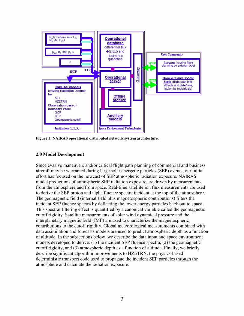
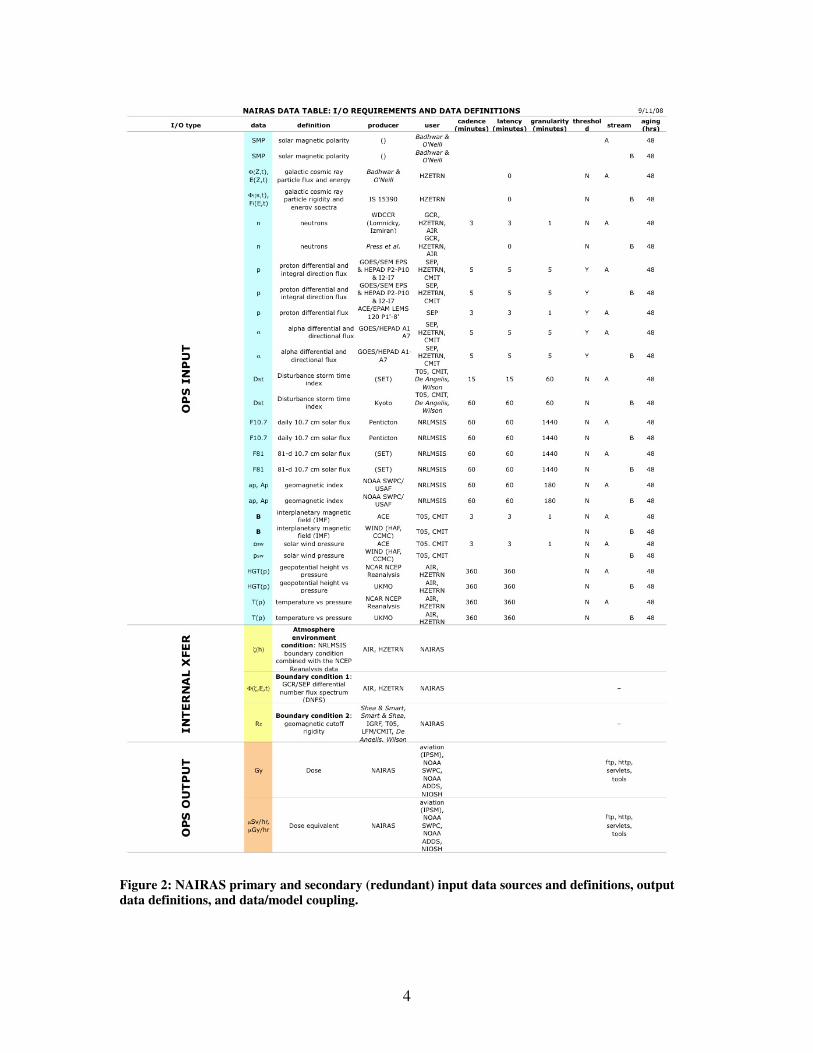
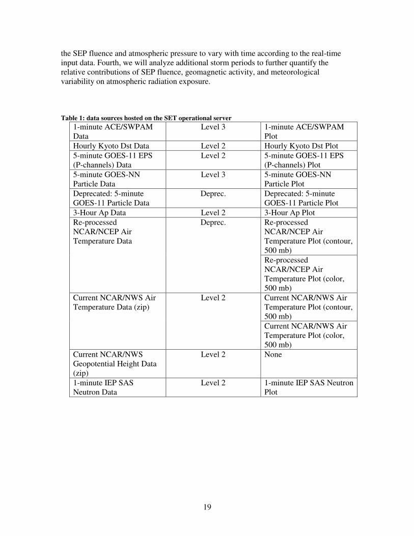
(Figure 1) is now a working prototype on an operational server. The primary and

secondary (redundant) input data sources (Table 1 and Figure 2) are now being gathered

continuously in a low cadence demonstration mode and provided from the current epoch

back through the past 4 days.

The risks for operationally incorporating redundant data streams have been identified

with the most significant outlier being the lack of availability of solar wind data in case

the ACE satellite goes off line. Both SET and the NOAA Space Weather Prediction

Center (SWPC) looked at this issue and the team concluded that the ENLIL plus cone

model may be a possible alternative, with the penalty of higher uncertainties, to supply

solar wind parameters in the event of ACE data loss. Other possible approaches are to

implement a data gap-fill algorithm, or calculate geomagnetic cutoff rigidities using a

simpler magnetospheric magnetic field model that utilizes a readily available

geomagnetic activity index (such as kp or Dst, for example). Each of these approaches

will be examined and evaluated in the coming months.

The SET preliminary Requirements Specification Document has been issued

as SET_report_1.pdf and it complements the I/O requirements along with data definitions

that have been established by the PI and SET team members as outlined in Figure 2.

Input data formats have been specified in algorithms and the data are being stored for 4

days in the database. A significant effort was required by SET to learn the format of

NCAR/NCEP and NCEP/NWS grib data files for tropospheric and stratospheric

parameters. The team was successful in interpreting and operationally incorporating these

data. The current epoch temperature at a given pressure level (examples of surface,

troposphere, and stratosphere) can be viewed at the http://spacewx.com site, SpWx

Now:Atmosphere Now menu items. The GOES particle data posed unique challenges:

SET was the beta-tester for the SPWC E-SWDS system (http://spacewx.com,

Innovation:E-SWDS menu item) whereby GOES data are now extracted directly from

NOAA servers and not the web portal. In the event E-SWDS fails, as has happened in

one or two cases as the system started up, SET's servers automatically go to the NOAA

web portal to retrieve data at a penalty of longer latency.

In addition to the operational server prototype, SET has established a password-protected

team website (http://sol.spacenvironment.net/~raps_ops/index.php) and a public website

(http://sol.spacenvironment.net/~nairas/index.html) for NAIRAS. Both sites will be used

for evolving NAIRAS to the next stage of test case model runs that access the SET

database for input data, and then provide output files to be picked up by the SET server

for deposit to the database. A task in the next year will be for each team member to help

define the requirements/data formats for his/her respective area of contribution and the

test cases will help us do this.

3

Figure 1: NAIRAS operational distributed network system architecture.

2.0 Model Development

Since evasive maneuvers and/or critical flight path planning of commercial and business

aircraft may be warranted during large solar energetic particles (SEP) events, our initial

effort has focused on the nowcast of SEP atmospheric radiation exposure. NAIRAS

model predictions of atmospheric SEP radiation exposure are driven by measurements

from the atmosphere and from space. Real-time satellite ion flux measurements are used

to derive the SEP proton and alpha fluence spectra incident at the top of the atmosphere.

The geomagnetic field (internal field plus magnetospheric contributions) filters the

incident SEP fluence spectra by deflecting the lower energy particles back out to space.

This spectral filtering effect is quantified by a canonical variable called the geomagnetic

cutoff rigidity. Satellite measurements of solar wind dynamical pressure and the

interplanetary magnetic field (IMF) are used to characterize the magnetospheric

contributions to the cutoff rigidity. Global meteorological measurements combined with

data assimilation and forecasts models are used to predict atmospheric depth as a function

of altitude. In the subsections below, we describe the data input and space environment

models developed to derive: (1) the incident SEP fluence spectra, (2) the geomagnetic

cutoff rigidity, and (3) atmospheric depth as a function of altitude. Finally, we briefly

describe significant algorithm improvements to HZETRN, the physics-based

deterministic transport code used to propagate the incident SEP particles through the

atmosphere and calculate the radiation exposure.

4

Figure 2: NAIRAS primary and secondary (redundant) input data sources and definitions, output

data definitions, and data/model coupling.

5

2.1 SEP Spectral Fluence

The NAIRAS model initially assumes a double power-law form for the SEP fluence

spectrum and derives fit parameters by a non-linear least-square fit to differential-

directional fluence measurements [Mewaldt et al., 2005]. The spectral fitting algorithm

uses a Marquardt-Levenberg iteration technique [Brandt, 1999]. If the double power-law

spectrum fails to converge to the measurement data, the fitting procedure is restarted and

the so-called Ellison-Ramaty spectral form is assumed [Ellison and Ramaty, 1985]. The

algorithm has been developed and tested on a number of storm periods.

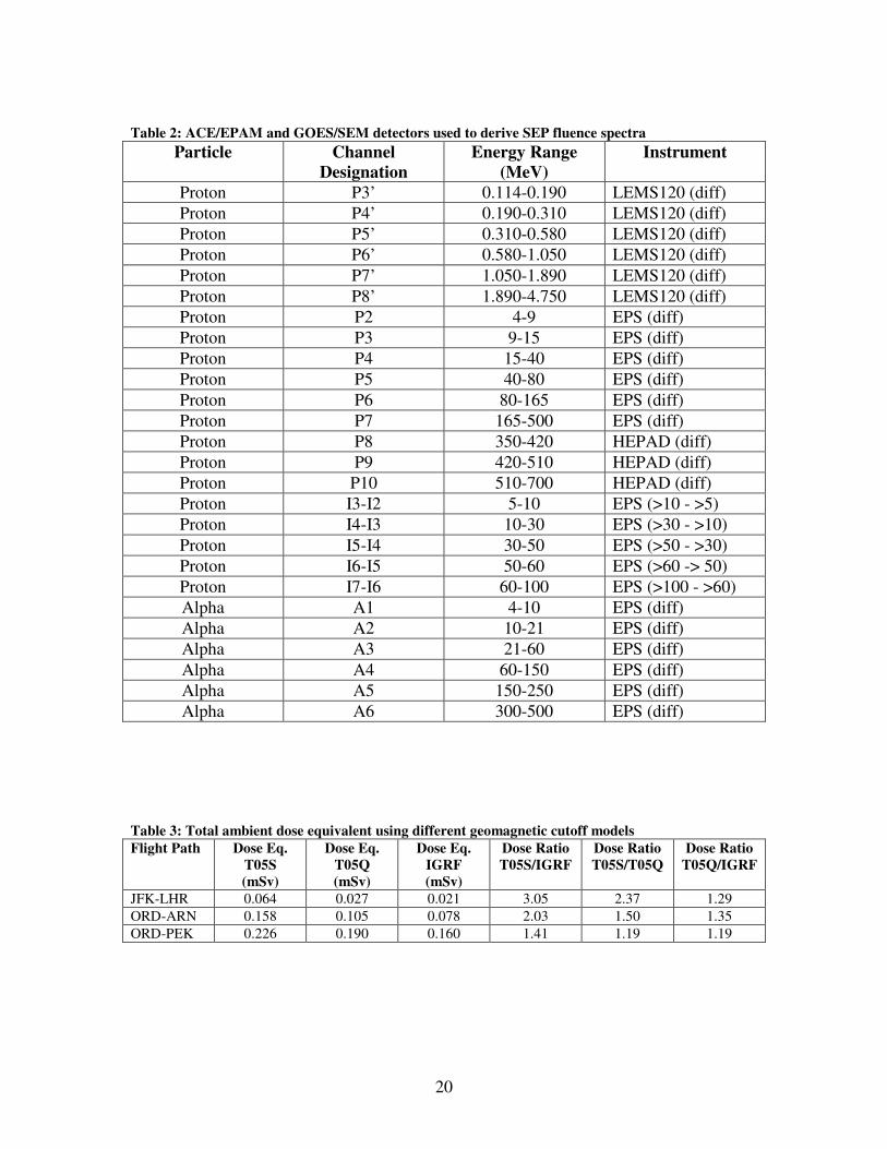
The NAIRAS model utilizes available real-time measurements of proton and alpha

differential-directional particle flux (cm2-sr-sec-MeV/n)

-1 for the SEP spectral fitting

described above. Fluence is obtained by time-integrating the particle flux measurements.

Low-energy proton data are obtained from the Electron, Proton, and Alpha Monitor

(EPAM) instrument onboard the NASA Advanced Composition Explorer (ACE) satellite

[Gold et al., 1998]. EPAM is composed of five telescopes and we use the LEMS120

(Low-Energy Magnetic Spectrometer) detector, which measures ions at 120 degrees from

the spacecraft axis. LEMS120 is the EPAM low-energy ion data available in real-time,

for reasons described by Haggerty et al. [2006]. The other proton channels used in the

SEP spectral fitting algorithm are obtained from NOAA's Geostationary Operational

Environmental Satellite (GOES) Space Environment Monitor (SEM) measurements. The

Energetic Particle Sensor (EPS) and the High Energy Proton and Alpha Detector

(HEPAD) sensors on GOES/SEM measure differential-directional proton flux [Onsager

et al., 1996]. We also generate additional differential proton measurement channels by

taking differences between the EPS integral proton flux channels. The channels used to

derive SEP alpha fluence spectra are also obtained from EPS measurements. We use 5-

minute averaged ACE and GOES data to derive the SEP fluence spectra.

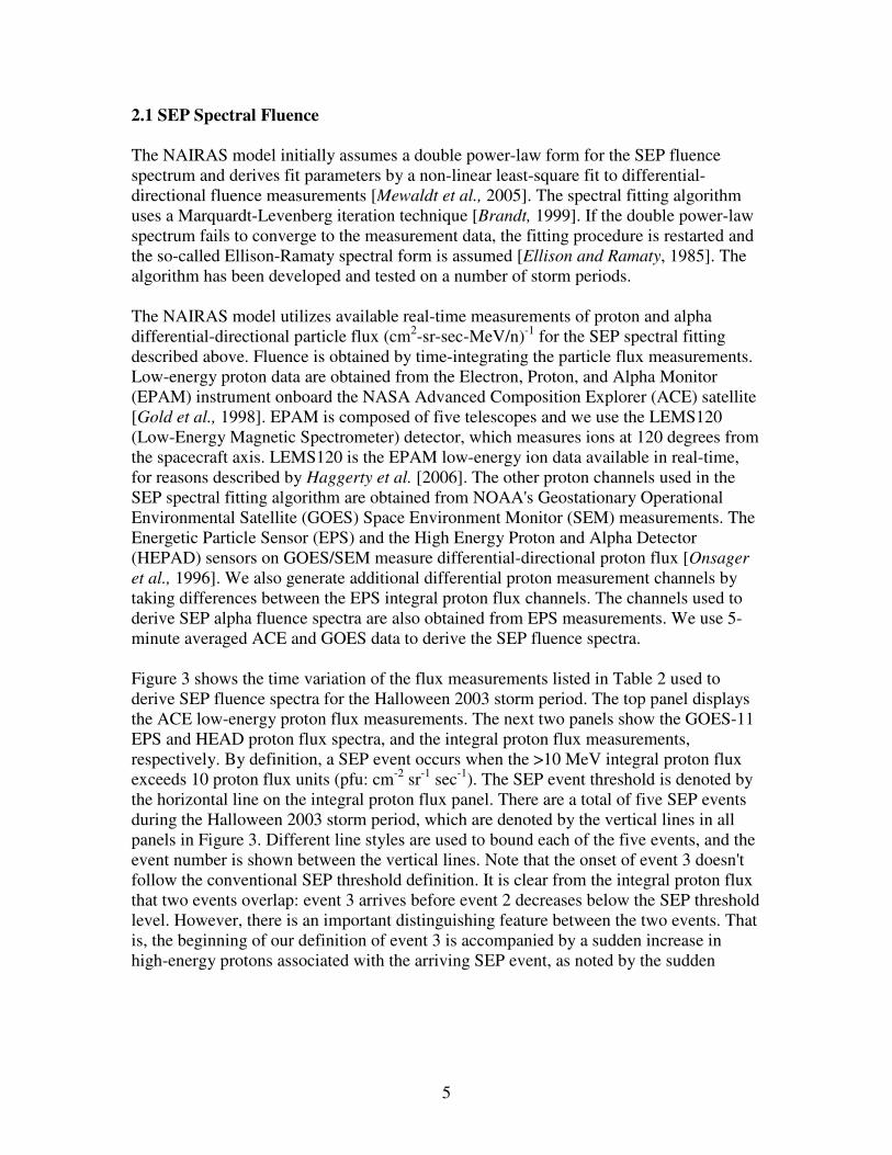
Figure 3 shows the time variation of the flux measurements listed in Table 2 used to

derive SEP fluence spectra for the Halloween 2003 storm period. The top panel displays

the ACE low-energy proton flux measurements. The next two panels show the GOES-11

EPS and HEAD proton flux spectra, and the integral proton flux measurements,

respectively. By definition, a SEP event occurs when the >10 MeV integral proton flux

exceeds 10 proton flux units (pfu: cm-2

sr-1

sec-1

). The SEP event threshold is denoted by

the horizontal line on the integral proton flux panel. There are a total of five SEP events

during the Halloween 2003 storm period, which are denoted by the vertical lines in all

panels in Figure 3. Different line styles are used to bound each of the five events, and the

event number is shown between the vertical lines. Note that the onset of event 3 doesn't

follow the conventional SEP threshold definition. It is clear from the integral proton flux

that two events overlap: event 3 arrives before event 2 decreases below the SEP threshold

level. However, there is an important distinguishing feature between the two events. That

is, the beginning of our definition of event 3 is accompanied by a sudden increase in

high-energy protons associated with the arriving SEP event, as noted by the sudden

6

Figure 3: Proton and alpha flux measurements used to derive the SEP fluence spectra. Row 1: ACE

EPAM/LEMS120 differential-directional proton flux measurements. Row 2: GOES-11 EPS and

HEPAD differential-directional proton flux measurements. Row 3: GOES-11 EPS integral-

directional proton flux measurements. Row 4: GOES-11 EPS differential-directional alpha flux

measurements. The different styled vertical lines bound the five SEP events during the Halloween

2003 solar-geomagnetic storm period, which are numbered in all panels. The horizontal line in Row 3

indicates the SEP threshold for the > 10 MeV integral proton flux channel.

increase in the 510-700 MeV differential proton flux measurements in Figure 3.

Partitioning the simultaneous SEP events 2 and 3 into separate events is useful for our

initial studies, since the high-energy portion of the differential proton flux distribution

penetrates deeper in the atmosphere.

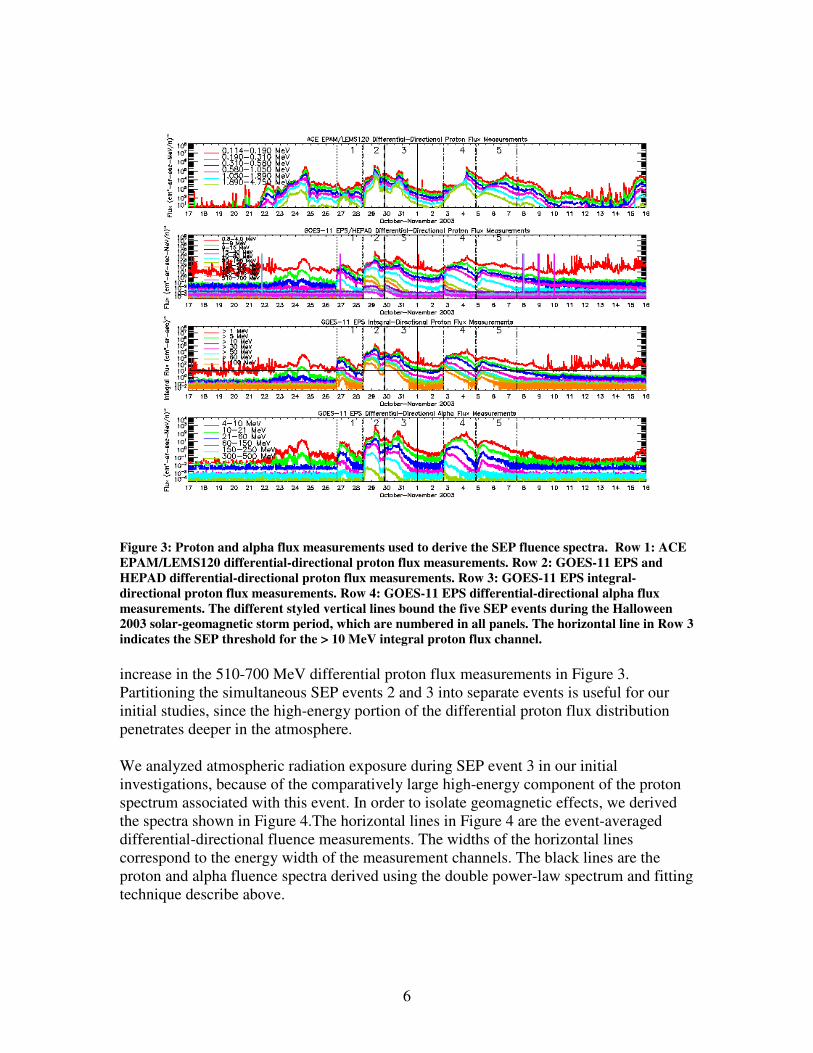
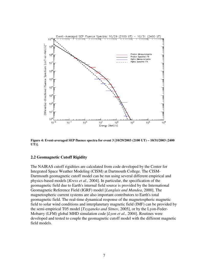
We analyzed atmospheric radiation exposure during SEP event 3 in our initial

investigations, because of the comparatively large high-energy component of the proton

spectrum associated with this event. In order to isolate geomagnetic effects, we derived

the spectra shown in Figure 4.The horizontal lines in Figure 4 are the event-averaged

differential-directional fluence measurements. The widths of the horizontal lines

correspond to the energy width of the measurement channels. The black lines are the

proton and alpha fluence spectra derived using the double power-law spectrum and fitting

technique describe above.

7

Figure 4: Event-averaged SEP fluence spectra for event 3 [10/29/2003 (2100 UT) – 10/31/2003 (2400

UT)].

2.2 Geomagnetic Cutoff Rigidity

The NAIRAS cutoff rigidities are calculated from code developed by the Center for

Integrated Space Weather Modeling (CISM) at Dartmouth College. The CISM-

Dartmouth geomagnetic cutoff model can be run using several different empirical and

physics-based models [Kress et al., 2004]. In particular, the specification of the

geomagnetic field due to Earth's internal field source is provided by the International

Geomagnetic Reference Field (IGRF) model [Langlais and Mandea, 2000]. The

magnetospheric current systems are also important contributors to Earth's total

geomagnetic field. The real-time dynamical response of the magnetospheric magnetic

field to solar wind conditions and interplanetary magnetic field (IMF) can be provided by

the semi-empirical T05 model [Tsyganeko and Sitnov, 2005], or by the Lyon-Feder-

Mobarry (LFM) global MHD simulation code [Lyon et al., 2004]. Routines were

developed and tested to couple the geomagnetic cutoff model with the different magnetic

field models.

8

10/27/03 10/29/03 10/31/03

50

55

60

65IG

RF

ma

gn

etic la

t. (

de

g)

UT hours

North enter

SAMPEX

TS05

10/27/03 10/29/03 10/31/03

50

55

60

65

IGR

F m

ag

ne

tic la

t. (

de

g)

UT hours

North exit

SAMPEX

TS05

10/27/03 10/29/03 10/31/03

50

55

60

65

AB

S I

GR

F m

ag

ne

tic la

t. (

de

g)

UT hours

South enter

SAMPEX

TS05

10/27/03 10/29/03 10/31/03

50

55

60

65

AB

S I

GR

F m

ag

ne

tic la

t. (

de

g)

UT hours

South exit

SAMPEX

TS05

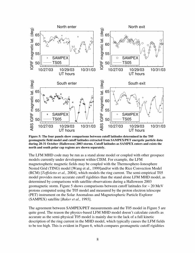
Figure 5: The four panels show comparisons between cutoff latitudes determined in the T05

geomagnetic field model and cutoff latitudes extracted from SAMPEX/PET energetic particle data

during 28-31 October (Halloween) 2003 storms. Cutoff latitudes as SAMPEX enters and exists the

north and south polar cap regions are shown separately.

The LFM MHD code may be run as a stand alone model or coupled with other geospace

models currently under development within CISM. For example, the LFM

magnetospheric magnetic fields may be coupled with the Thermosphere-Ionosphere

Nested Grid (TING) model [Wang et al., 1999]and/or with the Rice Convection Model

(RCM) [Toffoletto et al., 2004], which models the ring current. The semi-empirical T05

model provides more accurate cutoff rigidities than the stand alone LFM MHD model, as

determined by comparisons with satellite observations during a Halloween 2003

geomagnetic storm. Figure 5 shows comparisons between cutoff latitudes for ~ 20 MeV

protons computed using the T05 model and measured by the proton electron telescope

(PET) instrument on the Solar Anomalous and Magnetospheric Particle Explorer

(SAMPEX) satellite [Baker et al., 1993].

The agreement between SAMPEX/PET measurements and the T05 model in Figure 5 are

quite good. The reason the physics-based LFM MHD model doesn’t calculate cutoffs as

accurate as the semi-physical T05 model is mainly due to the lack of a full kinetic

description of the ring current in the MHD model, which typically causes the LFM fields

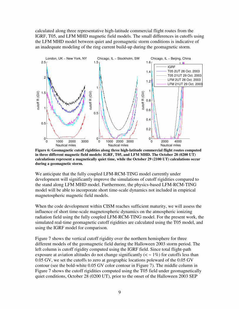
to be too high. This is evident in Figure 6, which compares geomagnetic cutoff rigidities

9

calculated along three representative high-latitude commercial flight routes from the

IGRF, T05, and LFM MHD magnetic field models. The small differences in cutoffs using

the LFM MHD model between quiet and geomagnetic storm conditions is indicative of

an inadequate modeling of the ring current build-up during the geomagnetic storm.

0 1000 2000 30000

0.5

1

1.5

2

2.5

Nautical miles

cu

toff

R (

GV

)

London, UK − New York, NY

0 1000 2000 30000

0.5

1

1.5

Nautical miles

cu

toff

R (

GV

)

Chicago, IL − Stockholm, SW

0 2000 40000

0.2

0.4

0.6

0.8

1

1.2

1.4

1.6

Nautical milescu

toff

R (

GV

)

Chicago, IL − Beijing, China

IGRF

T05 2UT 28 Oct. 2003

T05 21UT 29 Oct. 2003

LFM 2UT 28 Oct. 2003

LFM 21UT 29 Oct. 2003

Figure 6: Geomagnetic cutoff rigidities along three high-latitude commercial flight routes computed

in three different magnetic field models: IGRF, T05, and LFM MHD. The October 28 (0200 UT)

calculations represent a magnetically quiet time, while the October 29 (2100 UT) calculations occur

during a geomagnetic storm.

We anticipate that the fully coupled LFM-RCM-TING model currently under

development will significantly improve the simulations of cutoff rigidities compared to

the stand along LFM MHD model. Furthermore, the physics-based LFM-RCM-TING

model will be able to incorporate short time-scale dynamics not included in empirical

magnetospheric magnetic field models.

When the code development within CISM reaches sufficient maturity, we will assess the

influence of short time-scale magnetospheric dynamics on the atmospheric ionizing

radiation field using the fully coupled LFM-RCM-TING model. For the present work, the

simulated real-time geomagnetic cutoff rigidities are calculated using the T05 model, and

using the IGRF model for comparison.

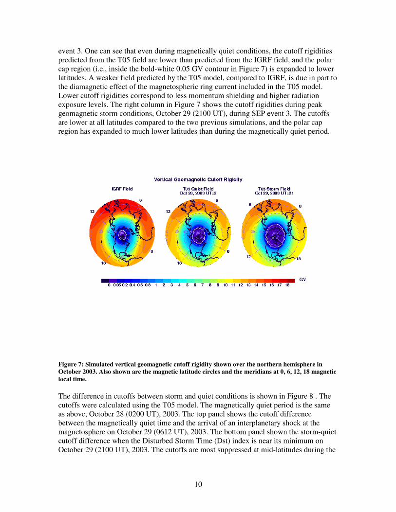
Figure 7 shows the vertical cutoff rigidity over the northern hemisphere for three

different models of the geomagnetic field during the Halloween 2003 storm period. The

left column is cutoff rigidity computed using the IGRF field. Since total flight-path

exposure at aviation altitudes do not change significantly (< ~ 1%) for cutoffs less than

0.05 GV, we set the cutoffs to zero at geographic locations poleward of the 0.05 GV

contour (see the bold-white 0.05 GV color contour in Figure 7). The middle column in

Figure 7 shows the cutoff rigidities computed using the T05 field under geomagnetically

quiet conditions, October 28 (0200 UT), prior to the onset of the Halloween 2003 SEP

10

event 3. One can see that even during magnetically quiet conditions, the cutoff rigidities

predicted from the T05 field are lower than predicted from the IGRF field, and the polar

cap region (i.e., inside the bold-white 0.05 GV contour in Figure 7) is expanded to lower

latitudes. A weaker field predicted by the T05 model, compared to IGRF, is due in part to

the diamagnetic effect of the magnetospheric ring current included in the T05 model.

Lower cutoff rigidities correspond to less momentum shielding and higher radiation

exposure levels. The right column in Figure 7 shows the cutoff rigidities during peak

geomagnetic storm conditions, October 29 (2100 UT), during SEP event 3. The cutoffs

are lower at all latitudes compared to the two previous simulations, and the polar cap

region has expanded to much lower latitudes than during the magnetically quiet period.

Figure 7: Simulated vertical geomagnetic cutoff rigidity shown over the northern hemisphere in

October 2003. Also shown are the magnetic latitude circles and the meridians at 0, 6, 12, 18 magnetic

local time.

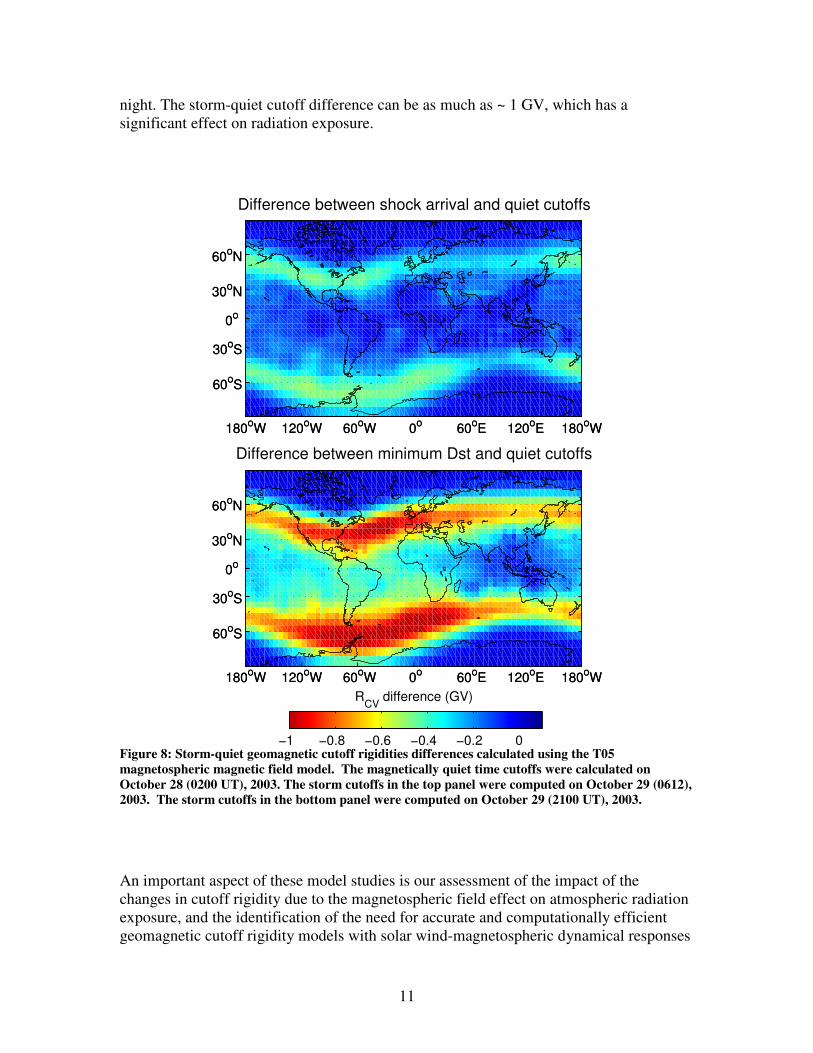
The difference in cutoffs between storm and quiet conditions is shown in Figure 8 . The

cutoffs were calculated using the T05 model. The magnetically quiet period is the same

as above, October 28 (0200 UT), 2003. The top panel shows the cutoff difference

between the magnetically quiet time and the arrival of an interplanetary shock at the

magnetosphere on October 29 (0612 UT), 2003. The bottom panel shown the storm-quiet

cutoff difference when the Disturbed Storm Time (Dst) index is near its minimum on

October 29 (2100 UT), 2003. The cutoffs are most suppressed at mid-latitudes during the

11

night. The storm-quiet cutoff difference can be as much as ~ 1 GV, which has a

significant effect on radiation exposure.

180oW 120

oW 60

oW 0

o 60

oE 120

oE 180

oW

60oS

30oS

0o

30oN

60oN

180oW 120

oW 60

oW 0

o 60

oE 120

oE 180

oW

60oS

30oS

0o

30oN

60oN

Difference between shock arrival and quiet cutoffs

RCV

difference (GV)

180oW 120

oW 60

oW 0

o 60

oE 120

oE 180

oW

60oS

30oS

0o

30oN

60oN

180oW 120

oW 60

oW 0

o 60

oE 120

oE 180

oW

60oS

30oS

0o

30oN

60oN

Difference between minimum Dst and quiet cutoffs

−1 −0.8 −0.6 −0.4 −0.2 0 Figure 8: Storm-quiet geomagnetic cutoff rigidities differences calculated using the T05

magnetospheric magnetic field model. The magnetically quiet time cutoffs were calculated on

October 28 (0200 UT), 2003. The storm cutoffs in the top panel were computed on October 29 (0612),

2003. The storm cutoffs in the bottom panel were computed on October 29 (2100 UT), 2003.

An important aspect of these model studies is our assessment of the impact of the

changes in cutoff rigidity due to the magnetospheric field effect on atmospheric radiation

exposure, and the identification of the need for accurate and computationally efficient

geomagnetic cutoff rigidity models with solar wind-magnetospheric dynamical responses

12

included. The ~ 1 GV suppression in cutoff at mid-latitudes during a geomagnetic storm

means that high-level SEP radiation exposure normally confined to the polar cap region

will be extended to mid-latitudes. More details of these findings are summarized in

section 3.0.

Considerable effort was applied to quantifying the minimum cutoff required in the

numerical simulations. Small cutoff rigidities require more computational time since the

time step in the numerical charged particle trajectory calculations in the geomagnetic

field are a fraction of the gyroperiod. Initially, we found that differences in accumulated

exposure for typical high-latitude flight paths are within 1% if the simulated cutoff

rigidity is set to zero for rigidities less than 0.05 GV. However, we found discontinuous

features in the exposure rates along the flight paths by setting the minimum cutoff to 0.05

GV. These discontinuities are suppressed if the minimum cutoff rigidity is set to 0.01

GV.

2.3 Meteorological Data

The atmospheric itself provides shielding from incident charged particles. The shielding

of the atmosphere at a given altitude depends on the overhead mass. Sub-daily global

atmospheric depth is determined from pressure versus geopotential height and pressure

versus temperature data derived from the National Center for Environmental Prediction

(NCEP) / National Center for Atmospheric Research (NCAR) Reanalysis 1 project

[Kalnay et al., 1996]. The NCAR/NCEP Reanalysis 1 project uses a state-of-the-art

analysis/forecast system to perform data assimilation using past data from 1948 to the

present. The data products are available 4x daily at 0, 6, 12, and 18 UT. The spatial

coverage is 17 pressure levels in the vertical from approximately the surface (1000 hPa)

to the middle stratosphere (10 hPa), while the horizontal grid is 2.5 x 2.5 degrees

covering the entire globe.

NCEP/NCAR pressure versus geopotential height data is extended in altitude above 10

hPa using the Naval Research Laboratory Mass Spectrometer and Incoherent Scatter

(NRLMSIS) model atmosphere [Picone et al., 2002]. NCEP/NCAR and NRLMSIS

temperatures are smoothly merged at 10 hPa at each horizontal grid point. NRLMSIS

temperatures are produced at 2 km vertical spacing from the altitude of the NCEP/NCAR

10 hPa pressure surface to approximately 100 km. The pressure at these extended

altitudes can be determined from the barometric law using the NRLMSIS temperature

profile and the known NCEP/NCAR 10 hPa pressure level, which assumes that the

atmosphere is in hydrostatic equilibrium and obeys the ideal gas law. Finally, the

altitudes and temperatures are linearly interpolated in log pressure to a fixed pressure grid

from 1000 hPa to 0.001 hPa, with six pressure levels per decade. The result from this step

is pressure versus altitude at each horizontal grid point from the surface to approximately

100 km.

Atmospheric depth (g/cm2) at each altitude level and horizontal grid point is computed by

vertically integrating the mass density from a given altitude to the top of the atmosphere.

The mass density is determined by the ideal gas law using the pressure and temperature at

13

each altitude level. The result from this step produces a 3-D gridded field of atmospheric

depth. Atmospheric depth at any specified aircraft altitude is determined by linear

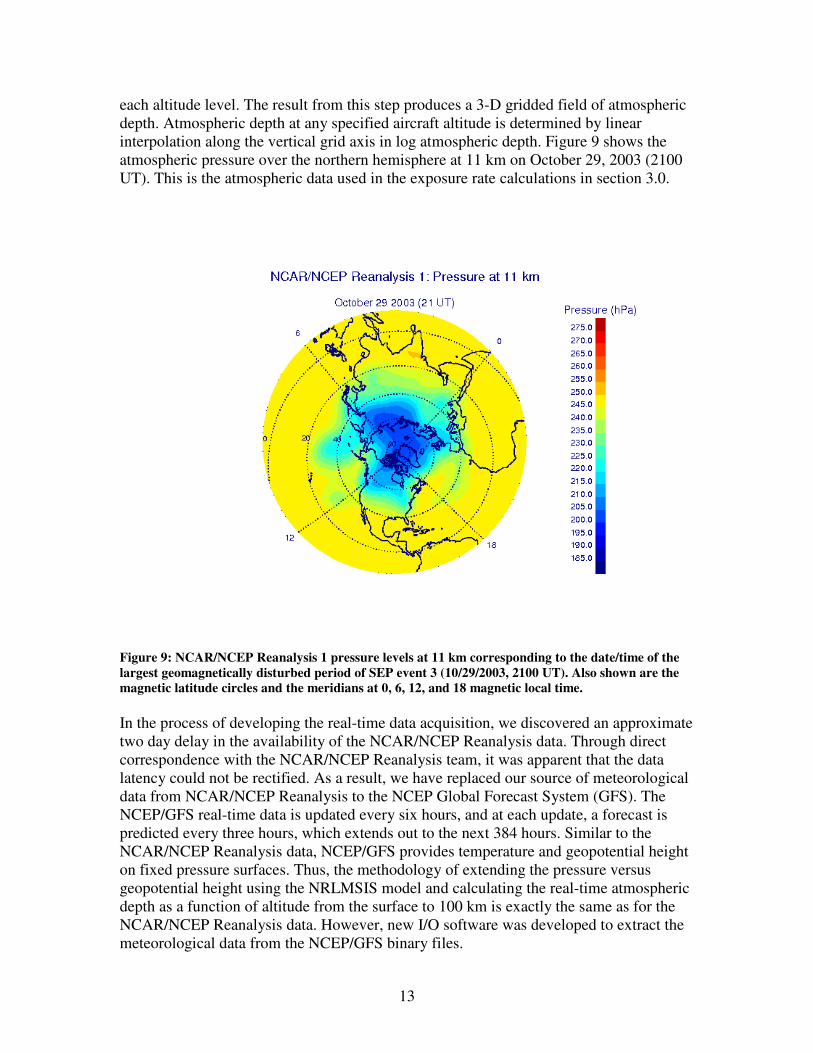
interpolation along the vertical grid axis in log atmospheric depth. Figure 9 shows the

atmospheric pressure over the northern hemisphere at 11 km on October 29, 2003 (2100

UT). This is the atmospheric data used in the exposure rate calculations in section 3.0.

Figure 9: NCAR/NCEP Reanalysis 1 pressure levels at 11 km corresponding to the date/time of the

largest geomagnetically disturbed period of SEP event 3 (10/29/2003, 2100 UT). Also shown are the

magnetic latitude circles and the meridians at 0, 6, 12, and 18 magnetic local time.

In the process of developing the real-time data acquisition, we discovered an approximate

two day delay in the availability of the NCAR/NCEP Reanalysis data. Through direct

correspondence with the NCAR/NCEP Reanalysis team, it was apparent that the data

latency could not be rectified. As a result, we have replaced our source of meteorological

data from NCAR/NCEP Reanalysis to the NCEP Global Forecast System (GFS). The

NCEP/GFS real-time data is updated every six hours, and at each update, a forecast is

predicted every three hours, which extends out to the next 384 hours. Similar to the

NCAR/NCEP Reanalysis data, NCEP/GFS provides temperature and geopotential height

on fixed pressure surfaces. Thus, the methodology of extending the pressure versus

geopotential height using the NRLMSIS model and calculating the real-time atmospheric

depth as a function of altitude from the surface to 100 km is exactly the same as for the

NCAR/NCEP Reanalysis data. However, new I/O software was developed to extract the

meteorological data from the NCEP/GFS binary files.

14

2.4 Low-Energy Neutron Transport

A recent update to HZETRN includes a directionally-coupled forward-backward low-

energy neutron transport algorithm, with coupling to light-ion transport [Slaba et al.,

2008]. The new deterministic transport algorithm was compared to Monte Carlo codes

HETC-HEDS, FLUKA, and MCNPX for the February, 1956 SEP event using the so-

called Webber spectrum. The new HZETRN neutron transport calculations agreed very

well with HETC-HEDS and reasonably well with FLUKA and MCNPX. The

comparisons showed significant improvements over the previous forward-backward

neutron transport model in HZETRN. The comparisons of the new deterministic neutron

transport model with the Monte Carlo codes verified that coupling between low-energy

neutrons and low-energy light-ion transport is not only necessary for accurate estimates

of the fluence spectra, but for integrated quantities such as dose and dose equivalent as

well.

The directionally-coupled forward-backward low-energy neutron transport algorithm

recently incorporated in HZETRN represents a significant improvement for physics-

based deterministic atmospheric ionizing radiation transport. For atmospheric radiation

exposure estimates, the new algorithm improved the accuracy of the contribution of

backscattered neutrons. The largest contribution from backscattered neutrons to dose

equivalent occurs in the region of typical commercial airline cruising altitudes.

3.0 Analysis of High-Energy SEP Event

Our initial model studies concentrated on predictions of SEP ambient dose equivalent

rates and accumulated ambient dose equivalent along representative high-latitude

commercial routes during the Halloween 2003 SEP event 3 [10/29 (2100 UT) - 10/31

(2400 UT)]. The incident SEP fluence and meteorological data were fixed in time in our

calculations, which are given by the event-averaged fluence and atmospheric depth-

altitude data shown in Figure 4 and Figure 9, respectively. On the other hand, we allowed

the cutoff rigidity to vary in time along the flight trajectories, according to the

magnetospheric magnetic field response to the real-time solar wind and IMF conditions.

A primary objective of this study was to diagnose geomagnetic storm effects on SEP

atmospheric radiation exposure. In the near future, we will allow the SEP fluence, cutoff

rigidity, and atmospheric depth-altitude to all vary according to the real-time data input.

Global SEP atmospheric radiation exposure is obtained from a pre-computed database.

The ambient dose equivalent rates are calculated on a fixed 2-D grid in atmospheric depth

and cutoff rigidity. The atmospheric depth grid extends from zero to 1300 g/cm2, and the

cutoff rigidity grid extends from zero to 19 GV. Both grids have non-uniform spacing

with the highest number of grid points weighted toward low cutoff rigidities and

tropospheric atmospheric depths. The real-time cutoff rigidities are computed on a 2.5 x

2.5 horizontal grid. The pre-computed ambient dose equivalent rates are interpolated to

the real-time cutoff rigidity and atmospheric depth specified at each horizontal grid point.

15

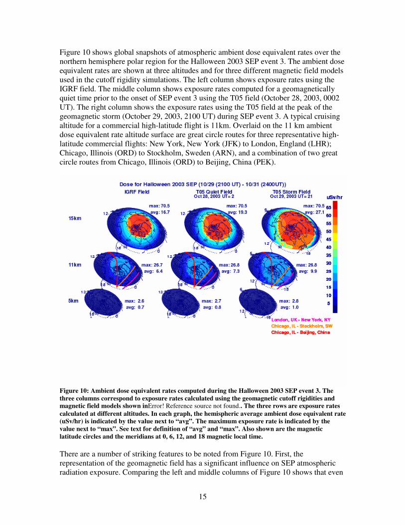
Figure 10 shows global snapshots of atmospheric ambient dose equivalent rates over the

northern hemisphere polar region for the Halloween 2003 SEP event 3. The ambient dose

equivalent rates are shown at three altitudes and for three different magnetic field models

used in the cutoff rigidity simulations. The left column shows exposure rates using the

IGRF field. The middle column shows exposure rates computed for a geomagnetically

quiet time prior to the onset of SEP event 3 using the T05 field (October 28, 2003, 0002

UT). The right column shows the exposure rates using the T05 field at the peak of the

geomagnetic storm (October 29, 2003, 2100 UT) during SEP event 3. A typical cruising

altitude for a commercial high-latitude flight is 11km. Overlaid on the 11 km ambient

dose equivalent rate altitude surface are great circle routes for three representative high-

latitude commercial flights: New York, New York (JFK) to London, England (LHR);

Chicago, Illinois (ORD) to Stockholm, Sweden (ARN), and a combination of two great

circle routes from Chicago, Illinois (ORD) to Beijing, China (PEK).

Figure 10: Ambient dose equivalent rates computed during the Halloween 2003 SEP event 3. The

three columns correspond to exposure rates calculated using the geomagnetic cutoff rigidities and

magnetic field models shown inError! Reference source not found.. The three rows are exposure rates

calculated at different altitudes. In each graph, the hemispheric average ambient dose equivalent rate

(uSv/hr) is indicated by the value next to “avg”. The maximum exposure rate is indicated by the

value next to “max”. See text for definition of “avg” and “max”. Also shown are the magnetic

latitude circles and the meridians at 0, 6, 12, and 18 magnetic local time.

There are a number of striking features to be noted from Figure 10. First, the

representation of the geomagnetic field has a significant influence on SEP atmospheric

radiation exposure. Comparing the left and middle columns of Figure 10 shows that even

16

during geomagnetically quiet periods, the magnetospheric magnetic field weakens the

overall geomagnetic field with a concomitant increase in radiation levels. This is seen as

a broadening of the open-closed magnetospheric boundary in the T05 quiet field

compared to the IGRF field. The cutoffs are zero in the region of open geomagnetic field

lines. Thus, ambient dose equivalent rates based on the IGRF field are underestimated

even for magnetically quiet times. During strong geomagnetic storms, as shown in the

third column of Figure 7, the area of open field lines are broadened further, bringing large

exposure rates to much lower latitudes. Ambient dose equivalent rates predicted using the

IGRF model during a large geomagnetic storm can be significantly underestimated. The

expansion of the polar region high exposure rates to lower latitudes, due to geomagnetic

effects, is quantified by calculating hemispheric average ambient dose equivalent rates

from 45N to the pole. This is denoted by “avg'' in Figure 10. At 11 km, there is roughly a

14% increase in the global-average ambient dose equivalent rate using T05 quiet-field

compared to IGRF. During the geomagnetic storm, there is a ~ 55% increase in the

global-average ambient dose equivalent rate using T05 storm-field compared to IGRF.

A second important feature to note in Figure 10 is the strong altitude dependence due to

atmospheric shielding. The exposure rates are very low at 5 km, independent of

geomagnetic field model used. At 15 km, the exposure rates are significantly higher than

at 11 km. Figure 10 shows that the SEP ambient dose equivalent rates increase (decrease)

exponentially with increasing (decreasing) altitude. The SEP exposure rate altitude

dependence is a fortunate feature for the aviation community, since radiation exposure

can be significantly reduced by descending to lower altitudes. Private business jets will

receive more radiation exposure than commercial aircraft if mitigation procedures are not

taken, since business jet cruising altitudes are roughly 12-13 km. The altitude dependence

of the SEP exposure rates are quantified in Figure 10 by showing the maximum ambient

dose equivalent rate at each altitude, which is the exposure rate at zero cutoff rigidity

(i.e., in the polar region of open geomagnetic field lines). The maximum is denoted

“max'' in Figure 10. The exposure rate increases on average by ~70% per km between 5

km and 11 km. Between 11 km and 15 km, the exposure rate increases on average by

approximately ~60% per km.

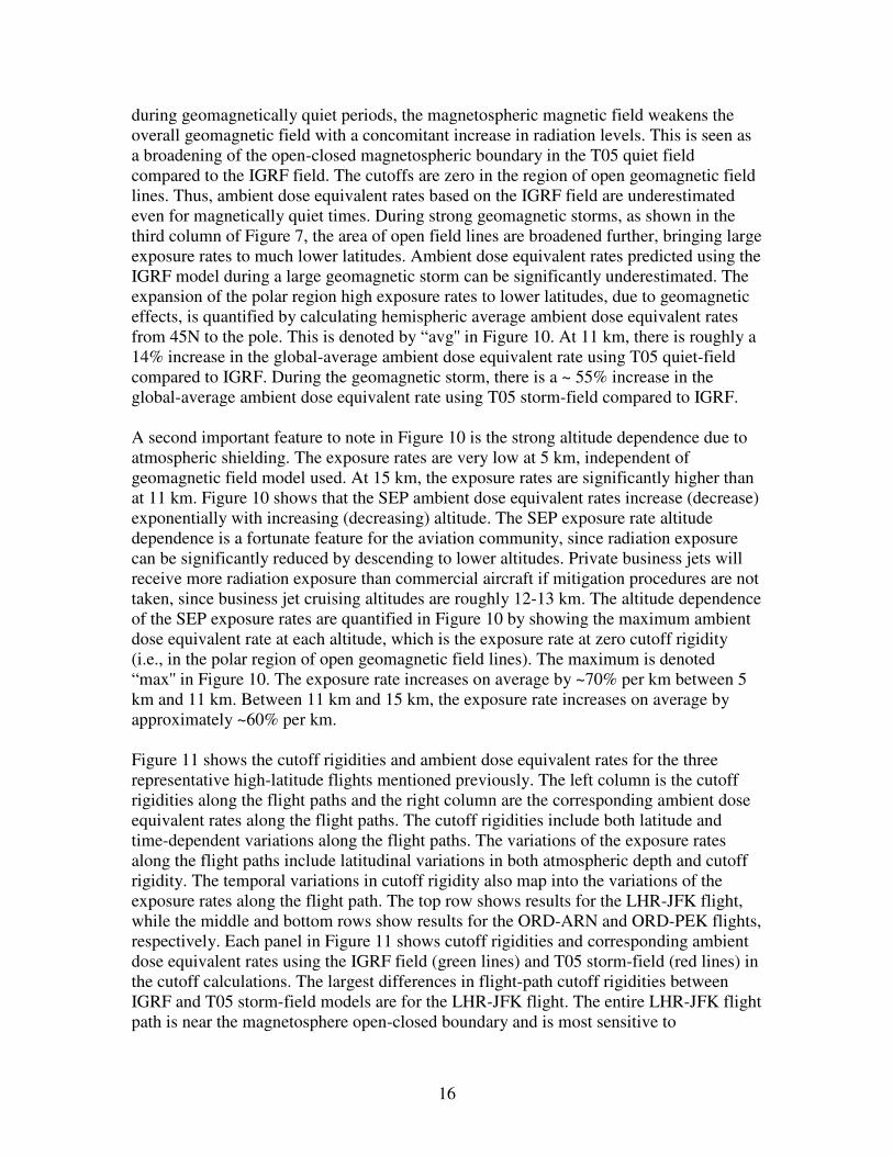
Figure 11 shows the cutoff rigidities and ambient dose equivalent rates for the three

representative high-latitude flights mentioned previously. The left column is the cutoff

rigidities along the flight paths and the right column are the corresponding ambient dose

equivalent rates along the flight paths. The cutoff rigidities include both latitude and

time-dependent variations along the flight paths. The variations of the exposure rates

along the flight paths include latitudinal variations in both atmospheric depth and cutoff

rigidity. The temporal variations in cutoff rigidity also map into the variations of the

exposure rates along the flight path. The top row shows results for the LHR-JFK flight,

while the middle and bottom rows show results for the ORD-ARN and ORD-PEK flights,

respectively. Each panel in Figure 11 shows cutoff rigidities and corresponding ambient

dose equivalent rates using the IGRF field (green lines) and T05 storm-field (red lines) in

the cutoff calculations. The largest differences in flight-path cutoff rigidities between

IGRF and T05 storm-field models are for the LHR-JFK flight. The entire LHR-JFK flight

path is near the magnetosphere open-closed boundary and is most sensitive to

17

perturbations in cutoff rigidity due to geomagnetic effects. Consequently, the exposure

rates along the LHR-JFK flight are most sensitive to geomagnetic effects. The ORD-PEK

polar route is the least sensitive to geomagnetic suppression of the cutoff rigidity, since

most of the flight path is across the polar cap region with open geomagnetic field lines.

The influence of geomagnetic storm effects on the ORD-ARN flight is intermediate

between a typical polar route and a flight along the North Atlantic corridor between the

US and Europe.

Figure 11: Geomagnetic cutoff rigidities (left column) and ambient dose equivalent rates (right

column) calculated during Halloween 2003 SEP event 3 along three representative flight paths for a

cruising altitude of 11 km. The green line represents cutoff rigidities and exposure rates calculated

using the IGRF model. The red lines represent cutoffs and exposure rates computed using the T05

model during the period of largest geomagnetic activity of event 3. Note that the ambient dose

equivalent rate calculated using the IGRF model for the LHR-JFK flight is scaled by a factor of two.

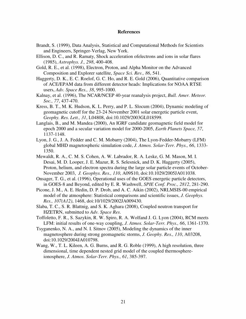
The total ambient dose equivalent along the three representative high-latitude flight paths

is given in Table 3. The first three columns show total ambient dose equivalent computed

from the three models of the geomagnetic field used in this study: IGRF, T05 quiet-field,

and T05 storm-field. The last three columns show various ratios between the total

ambient dose equivalent computed from the different geomagnetic field models. There

are three major points to be noted from these results. One, the total ambient dose

equivalent predicted for the ORD-PEK polar route for SEP event 3 during the Halloween

2003 storm reaches 22% of ICRP public/prenatal effective dose limit of 1 mSv. Two,

18

using the IGRF field to compute the cutoff rigidity can underestimate the total ambient

dose equivalent from ~ 40% for polar routes to over a factor of three for flights along the

North Atlantic corridor. Third, even for SEP events without an accompanying

geomagnetic storm, using the IGRF field in cutoff rigidity simulations can underestimate

the total ambient dose equivalent by roughly 30% for US flights into Europe.

In this initial study we have conducted an analysis of atmospheric ionizing radiation

exposure associated with a high-energy SEP event during the Halloween 2003 storm

period. The two main objectives of this analysis are the following: (1) provide an

estimate of the exposure received on representative high-latitude commercial flights

during the high-energy SEP event, and (2) to diagnose the influence of geomagnetic

storm effects on SEP atmospheric radiation exposure. High-latitude flight paths are the

routes most susceptible to significant SEP radiation exposure, since the cutoff rigidity

rapidly approaches zero near the magnetosphere open-closed boundary.

The result from our first objective is that the radiation exposure during a representative

polar flight was 22% of the ICRP public/prenatal limit. SEP exposure rates increase

(decrease) exponentially with increasing (decreasing) altitude. Thus, SEP aircraft

radiation exposure can be significantly reduced by descending to lower altitudes.

Business jet cruising altitudes are higher than commercial aircraft. Consequently, private

jets flying similar high-latitude routes as the commercial airlines will receive

substantially more radiation if mitigation procedures are not enacted. NAIRAS real-time

radiation exposure rate predictions during SEP events will enable the aviation community

to make informed decisions concerning radiation risk evaluation and reduction.

To achieve our second objective of diagnosing the geomagnetic storm effects on SEP

radiation exposure, we calculated the atmospheric ambient dose equivalent rates using

event-averaged incident SEP proton and alpha fluence spectra and a static atmospheric

depth-altitude relation, while the cutoff rigidity was calculated both statically and

dynamically. The static cutoff rigidities were simulated using the IGRF field. The

dynamic cutoff rigidities were simulated using the T05 field, which was allowed to

respond to the real-time solar wind and IMF conditions. The dynamic cutoff rigidities

were computed during a geomagnetically quiet period prior to the high-energy SEP event

and during the peak of the geomagnetic storm associated with the high-energy SEP event.

The key results of this study are as follows. One, ignoring solar wind-magnetosphere

interactions during a strong geomagnetic storm in the calculation of cutoff rigidity can

underestimate the total exposure by approximately 40% to over a factor of three. Two,

even during geomagnetically quiet conditions, ignoring solar wind-magnetosphere

interactions in the computed cutoff rigidities can underestimate the total exposure for

flights along the North Atlantic corridor by roughly 30%. To achieve more accurate

assessments of aircraft radiation exposure, the magnetospheric influence on the cutoff

rigidities must be included routinely in atmospheric radiation exposure predictions.

Our future efforts will build upon this work in four ways. One, we will study directional

effects on the cutoff rigidities and subsequent radiation exposure rates. Two, we will

model the aircraft fuselage and full body organ and tissue exposure. Third, we will allow

19

the SEP fluence and atmospheric pressure to vary with time according to the real-time

input data. Fourth, we will analyze additional storm periods to further quantify the

relative contributions of SEP fluence, geomagnetic activity, and meteorological

variability on atmospheric radiation exposure.

Table 1: data sources hosted on the SET operational server

1-minute ACE/SWPAM

Data

Level 3 1-minute ACE/SWPAM

Plot

Hourly Kyoto Dst Data Level 2 Hourly Kyoto Dst Plot

5-minute GOES-11 EPS

(P-channels) Data

Level 2 5-minute GOES-11 EPS

(P-channels) Plot

5-minute GOES-NN

Particle Data

Level 3 5-minute GOES-NN

Particle Plot

Deprecated: 5-minute

GOES-11 Particle Data

Deprec. Deprecated: 5-minute

GOES-11 Particle Plot

3-Hour Ap Data Level 2 3-Hour Ap Plot

Re-processed

NCAR/NCEP Air

Temperature Plot (contour,

500 mb)

Re-processed

NCAR/NCEP Air

Temperature Data

Deprec.

Re-processed

NCAR/NCEP Air

Temperature Plot (color,

500 mb)

Current NCAR/NWS Air

Temperature Plot (contour,

500 mb)


Temperature Data (zip)

Level 2


Temperature Plot (color,

500 mb)

Current NCAR/NWS

Geopotential Height Data

(zip)

Level 2 None

1-minute IEP SAS

Neutron Data

Level 2 1-minute IEP SAS Neutron

Plot

20

Table 2: ACE/EPAM and GOES/SEM detectors used to derive SEP fluence spectra

Particle Channel

Designation

Energy Range

(MeV)

Instrument

Proton P3’ 0.114-0.190 LEMS120 (diff)






Proton P2 4-9 EPS (diff)






Proton P8 350-420 HEPAD (diff)



Proton I3-I2 5-10 EPS (>10 - >5)

Proton I4-I3 10-30 EPS (>30 - >10)

Proton I5-I4 30-50 EPS (>50 - >30)

Proton I6-I5 50-60 EPS (>60 -> 50)

Proton I7-I6 60-100 EPS (>100 - >60)

Alpha A1 4-10 EPS (diff)






Table 3: Total ambient dose equivalent using different geomagnetic cutoff models

Flight Path Dose Eq.

T05S

(mSv)

Dose Eq.

T05Q

(mSv)

Dose Eq.

IGRF

(mSv)

Dose Ratio

T05S/IGRF

Dose Ratio

T05S/T05Q

Dose Ratio

T05Q/IGRF

JFK-LHR 0.064 0.027 0.021 3.05 2.37 1.29

ORD-ARN 0.158 0.105 0.078 2.03 1.50 1.35

ORD-PEK 0.226 0.190 0.160 1.41 1.19 1.19

21

References

Brandt, S. (1999), Data Analysis, Statistical and Computational Methods for Scientists

and Engineers, Springer-Verlag, New York.

Ellison, D. C., and R. Ramaty, Shock acceleration ofelectrons and ions in solar flares

(1985), Astrophys. J., 298, 400-408.

Gold, R. E., et al. (1998), Electron, Proton, and Alpha Monitor on the Advanced

Composition and Explorer satellite, Space Sci. Rev., 86, 541.

Haggerty, D. K., E. C. Roelof, G. C. Ho, and R. E. Gold (2006), Quantitative comparison

of ACE/EPAM data from different detector heads: Implications for NOAA RTSE

users, Adv. Space Res., 38, 995-1000.

Kalnay, et al. (1996), The NCAR/NCEP 40-year reanalysis project, Bull. Amer. Meteor.

Soc., 77, 437-470.

Kress, B. T., M. K. Hudson, K. L. Perry, and P. L. Slocum (2004), Dynamic modeling of

geomagnetic cutoff for the 23-24 November 2001 solar energetic particle event,

Geophy. Res. Lett., 31, L04808, doi:10.1029/2003GL018599.

Langlais, B., and M. Mandea (2000), An IGRF candidate geomagnetic field model for

epoch 2000 and a secular variation model for 2000-2005, Earth Planets Space, 57,

1137-1148.

Lyon, J. G., J. A. Fedder and C. M. Mobarry (2004), The Lyon-Fedder-Mobarry (LFM)

global MHD magnetospheric simulation code, J. Atmos. Solar-Terr. Phys., 66, 1333-

1350.

Mewaldt, R. A., C. M. S. Cohen, A. W. Labrador, R. A. Leske, G. M. Mason, M. I.

Desai, M. D. Looper, J. E. Mazur, R. S. Selesnick, and D. K. Haggerty (2005),

Proton, helium, and electron spectra during the large solar particle events of October-

November 2003, J. Geophys. Res., 110, A09S10, doi:10.1029/2005JA011038.

Onsager, T. G., et al. (1996), Operational uses of the GOES energetic particle detectors,

in GOES-8 and Beyond, edited by E. R. Washwell, SPIE Conf. Proc., 2812, 281-290.

Picone, J. M., A. E. Hedin, D. P. Drob, and A. C. Aikin (2002), NRLMSIS-00 empirical

model of the atmosphere: Statistical comparisons and scientific issues, J. Geophys.

Res., 107(A12), 1468, doi:10/1029/2002JA009430.

Slaba, T. C., S. R. Blattnig, and S. K. Aghara (2008), Coupled neutron transport for

HZETRN, submitted to Adv. Space Res.

Toffoletto, F. R., S. Sazykin, R. W. Spiro, R. A. Wolfand J. G. Lyon (2004), RCM meets

LFM: initial results of one-way coupling, J. Atmos. Solar-Terr. Phys., 66, 1361-1370.

Tsyganenko, N. A., and N. I. Sitnov (2005), Modeling the dynamics of the inner

magnetosphere during strong geomagnetic storms, J. Geophy. Res., 110, A03208,

doi:10.1029/2004JA010798.

Wang, W., T. L. Kileen, A. G. Burns, and R. G. Roble (1999), A high resolution, three

dimensional, time dependent nested grid model of the coupled thermosphere-

ionosphere, J. Atmos. Solar-Terr. Phys., 61, 385-397.

Documents

Development of Nowcast of Atmospheric Ionizing Radiation for