Development of models for designing industrial energy technologies related to cold production and storage Master’s Thesis within the Sustainable Energy Systems programme

RÉMI ALLET EDF R&D Department of Eco-Energy Efficiency and Industrial Processes Moret-sur-Loing, France Department of Energy and Environment Division of Heat and Power Technology CHALMERS UNIVERSITY OF TECHNOLOGY Göteborg, Sweden 2011

MASTER’S THESIS

Development of models for designing industrial energy technologies related to

cold production and storage

Master’s Thesis within the Sustainable Energy Systems programme

RÉMI ALLET

SUPERVISOR(S):

Stéphanie Jumel (EDF)

Mathias Gourdon (Chalmers)

EXAMINER

Mathias Gourdon

Department of Energy and Environment Division of Heat and Power Technology

CHALMERS UNIVERSITY OF TECHNOLOGY

Göteborg, Sweden 2011

Development of models for designing industrial energy technologies related to cold production and storage Master’s Thesis within the Sustainable Energy Systems programme RÉMI ALLET

© RÉMI ALLET, 2011

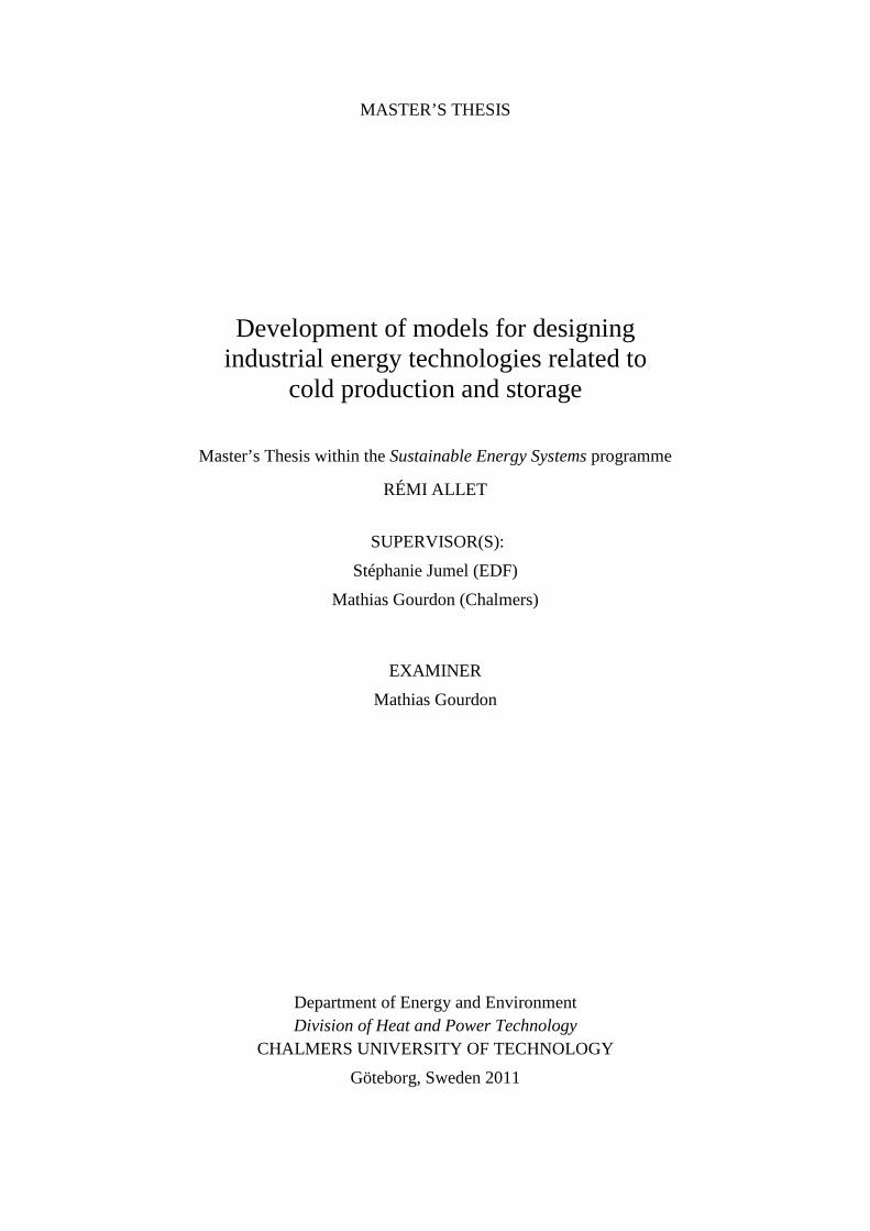
Department of Energy and Environment Division of Heat and Power Technology Chalmers University of Technology SE-412 96 Göteborg Sweden Telephone: + 46 (0)31-772 1000 Cover: Experimental refrigerator of the E25 laboratories located at the research centre EDF Les Renardières, Moret-sur-Loing, France. Chalmers Reproservice Göteborg, Sweden 2011

I

Development of models for designing industrial energy technologies related to cold production and storage Master’s Thesis in the Sustainable Energy Systems programme RÉMI ALLET Department of Energy and Environment Division of Heat and Power Technology Chalmers University of Technology

ABSTRACT

Numerous industries use cold fluids in their processes. Large energy savings can be achieved through the efficient use of technologies such as refrigerators and cold storage. However, their integration requires detailed studies to fit the network and the demand. A simulation tool is often an asset to estimate the performance of a system.

The objective of this thesis is to develop models related to cold production and storage, allowing a user to assess systems’ design and performances through dynamic simulations. The work is based on the Modelica/Dymola environment. The Modelica language offers an innovative way to model systems by using equations instead of assignment statements. Due to this acausality, the same model can have multiple purposes.

The technologies modelled are a refrigerator, a combined refrigerator/heat pump and a latent heat storage with spherical phase-change material (PCM) capsules. The refrigerator and the combined refrigerator/heat pump are an assembling of four components that are also modelled: a compressor, a condenser, an expansion valve, and an evaporator. The development followed strict rules that allow a user to include these components in a larger network with other systems.

The performance of the models was assessed during test cases. They reveal a good accuracy of the results, from a theoretical and experimental point of view. Some difficulties were encountered, most of them due to the nature of the language or the way the refrigerant properties were retrieved for calculations. The models are however functional for most of the industrial studies.

Applications for the developed models are various. They can be used to assess the performance of an existing or future network. They also authorize sensitivity analysis thanks to their easy-to-configure parameters. Finally, they are also suitable for designing equipment. One example in the thesis describes the combination of a refrigerator and a cold storage which adapt their production according to a cooling demand.

Key words: cold production, refrigerator, storage, phase-change material, modelling, simulation, Modelica, Dymola

II

III

Contents ABSTRACT I

CONTENTS III

PREFACE VII

NOTATIONS VIII

1 INTRODUCTION 1

1.1 Presentation of EDF 1

1.2 Background 1

1.3 Objectives 2

1.4 Methodology 3

2 PRESENTATION OF MODELICA AND DYMOLA 5

2.1 The Modelica language 5

2.1.1 General introduction 5

2.1.2 Basic programming concepts 5

2.2 The Dymola environment 7

2.2.1 General introduction 7

2.2.2 Presentation of the environment 8

2.2.3 Assembling components 9

2.2.4 Model settings and preparation to the simulation 10

2.2.5 Simulation and visualization of results 11

3 GENERAL PRINCIPLES AND MODELS 13

3.1 Development rules 13

3.2 Connectors 13

3.3 Loop breakers 14

3.4 Sources and sinks 14

3.4.1 Basic source and sink 15

3.4.2 Timetable and source with external input 16

3.5 Thermodynamic properties of fluids 17

3.5.1 External executable 17

3.5.2 Dynamic library 18

3.5.3 Polynomial functions 19

4 REFRIGERATOR MODELLING 21

4.1 Presentation of the technology 21

4.1.1 Regulation 23

4.1.2 Refrigerator variants 23

4.2 Mathematical models 24

4.2.1 Compressor 25

IV

4.2.2 Condenser 26

4.2.3 Evaporator 28

4.2.4 Expansion valve 29

4.3 Modelica models 30

4.3.1 Components 30

4.3.2 Refrigerator 31

4.3.3 Combined refrigerator/heat pump 32

4.4 Simulations and results 33

4.4.1 Test case 33

4.4.2 Experimental case 34

5 COLD STORAGE MODELLING 37

5.1 Presentation of the technology 37

5.1.1 Mechanism 38

5.1.2 Performance 38

5.2 Mathematical model 39

5.2.1 Hypotheses 39

5.2.2 Parameters 39

5.2.3 Variables 41

5.2.4 Mesh 43

5.2.5 Equations 44

5.3 Modelica model 48

5.4 Simulations and results 49

6 REFRIGERATOR AND COLD STORAGE COMBINATION 53

6.1 Description of the modes of operation 53

6.1.1 Charge only 54

6.1.2 Direct production 54

6.1.3 Discharge only 55

6.1.4 Direct production and discharge 55

6.1.5 Direct production and charge 56

6.2 Regulation 56

6.3 Modelica model 56

6.4 Simulations and results 60

7 DISCUSSION 64

7.1 Comments on hypotheses 64

7.1.1 Compressor efficiencies 64

7.1.2 ∆Tmin position 64

7.1.3 Constant fluid properties 64

7.1.4 PCM conductivity 65

7.2 Perspectives regarding the developed models 66

7.3 Improvements and further work 66

7.3.1 Systems design 66

V

7.3.2 Optimization of operating modes for a cold production 67 7.3.3 Compressor working limits 67

7.3.4 ∆Tmin value 67

7.3.5 Temperature inertia 68

8 CONCLUSION 69

9 REFERENCES 70

APPENDIX 1: GENERAL MODELS 73

Connector 73

Source 73

Loop breaker 74

Valve with 2 inlets and 1 outlet 74

APPENDIX 2: REFRIGERATOR MODELICA MODELS 75

Compressor 75

Condenser 75

Evaporator 75

Expansion valve 75

Refrigerator 75

Combined refrigerator/heat pump 75

APPENDIX 3: STORAGE MODELICA MODELS 76

VI

VII

Preface This thesis has been carried out between February and July 2011 at the research centre EDF Les Renardières, Moret-sur-Loing, France. The work conducted is a part of a research project aiming at the creation of a library of industrial energy technologies that started a few years ago. The overall project is financed by the French company EDF (Electricité de France).

This study uses the computer language Modelica developed by the Modelica Association, along with the software Dymola developed by Dassault Systèmes.

A large part of this work could not have been possible without the help of the EDF staff. I would like to thank all the people I had the opportunity to meet and work with, it has been a rewarding experience. My greatest gratitude goes to the people of the group E26 with which I shared the same offices during six months. I would especially like to thank my supervisor Stéphanie Jumel for her sympathy and availability; Fabienne Pingal for her warm welcome and kindness throughout the thesis; and Grégoire Duhot for his scientific and technical proficiency regarding the studied technologies, he has been a great help.

Finally, I would like to truly thank Mathias Gourdon, my Chalmers supervisor and examiner. Despite the distance between us, he has always been available to assist and guide me during the thesis. His reactivity and his involvement have been a real asset.

Moret-sur-Loing, August 2011

Rémi Allet

VIII

Notations HTF Heat transfer fluid PCM Phase-change material � Area of contact between two elements (m²) �� Specific heat capacity (kJ/kg.K)) � Thickness (m) �� Mass in one element (kg) �� Exchange surface of one element (m²) �� Volume of one element (m3) � Diameter (m) Volume fraction filled by the HTF ℎ Specific enthalpy (kJ/kg) ℎ� Convective coefficient of heat transfer (W/(m².K)) I Thermal insulance (m².K/W) � Thermal conductivity (W/(m.K)) Length (m) � Mass flow rate (kg/s) � Number of elements � Number of nodules �� Nusselt number � Pressure (bar) �� Prandtl number � Heat rate (kW), heat gain (kJ) � Radius (m) �� Reynolds number � Specific entropy (kJ/(kg.K)) � Surface (m²) � Time (s) � Temperature (K) � Velocity (m/s) � Overall heat transfer coefficient (W/(m².K)) � Volume (m3) � Power (kW) � Steam mass fraction, length (m) �� PCM liquid fraction

Greek symbols Δ Difference � Efficiency � Kinematic viscosity Pressure ratio ! Density

Subscripts 0 Initial 1 Compressor inlet

IX

2 Compressor outlet 2� After isentropic compression 3 Condenser outlet 4 Evaporator inlet ', '�) Ambient '*� Air +ℎ'�,� Charge +-�� Compressor +-�� Condensation � Distribution ��� Demand ��ℎ Desuperheating � External fluid �, External fluid when refrigerant is at saturated vapour �.'� Evaporation ��� External fluid on the condenser side Refrigerant, HTF Refrigerant at saturated liquid , Refrigerant at saturated vapour ,/0+-/ Water-glycol ℎ� Exchanged ℎ1��- Reference for zero enthalpy *, *� Inlet *�* Difference between initial and reference *� Isentropic Liquid PCM � Mechanical �'� Maximum �*� Minimum �*�+ Minimum in condenser �*�� Minimum in evaporator �-� Nodule �-� Nominal -, -�� Outlet �, �+� PCM 21��- Reference for no heat stored �� Refrigerant, refrigerator � Storage, solid �'� Saturation, phase-change, latent �'� Liquid saturation �'�� Solid saturation �+ Subcooling �ℎ Superheating ��- Storage ��-��� Stored in the tank � Solid PCM 3,3'// Tank wall 3'��� Water

1

1 Introduction 1.1 Presentation of EDF The EDF Group is a leading player in the European energy industry and a leader in the French electricity market, active in all areas of the electricity value chain, from generation to trading, and increasingly active in the gas market in Europe. Leader in the French electricity market, the Group also has solid positions in the United Kingdom, Italy and numerous other European countries, as well as industrial operations in Asia and the United States. Over the years, it has become the first nuclear operator worldwide and the first hydropower producer in Europe, generating 630 TWh of electricity in 2010.

EDF is relying on the power of innovation to meet the world’s energy challenges. That’s why the EDF invests about €490 million/year and employs 2,000 people in its Research and Development division. Generation, networks and customers energy uses: R&D is improving performance in all EDF businesses and works on the modernization of infrastructures to optimize both output and safety. The development of low-carbon electricity is the R&D’s core focus. Its goal is to accelerate the transition from innovation to industrial commercialization on the market.

EDF R&D is divided into 15 departments corresponding to 15 fields of activity, which are split between 5 research centres: 3 near Paris (France), 1 in London (UK), and 1 in Karlsruhe (Germany).

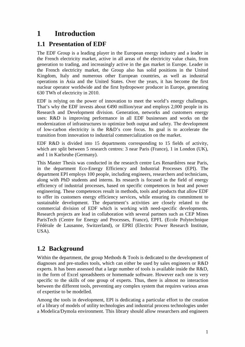
This Master Thesis was conducted in the research centre Les Renardières near Paris, in the department Eco-Energy Efficiency and Industrial Processes (EPI). The department EPI employs 100 people, including engineers, researchers and technicians, along with PhD students and interns. Its research is focused in the field of energy efficiency of industrial processes, based on specific competences in heat and power engineering. These competences result in methods, tools and products that allow EDF to offer its customers energy efficiency services, while ensuring its commitment to sustainable development. The department’s activities are closely related to the commercial division of EDF which is working with need-specific developments. Research projects are lead in collaboration with several partners such as CEP Mines ParisTech (Centre for Energy and Processes, France), EPFL (Ecole Polytechnique Fédérale de Lausanne, Switzerland), or EPRI (Electric Power Research Institute, USA).

1.2 Background Within the department, the group Methods & Tools is dedicated to the development of diagnoses and pre-studies tools, which can either be used by sales engineers or R&D experts. It has been assessed that a large number of tools is available inside the R&D, in the form of Excel spreadsheets or homemade software. However each one is very specific to the skills of one group of experts. Thus, there is almost no interaction between the different tools, preventing any complex system that requires various areas of expertise to be modelled.

Among the tools in development, EPI is dedicating a particular effort to the creation of a library of models of utility technologies and industrial process technologies under a Modelica/Dymola environment. This library should allow researchers and engineers

2

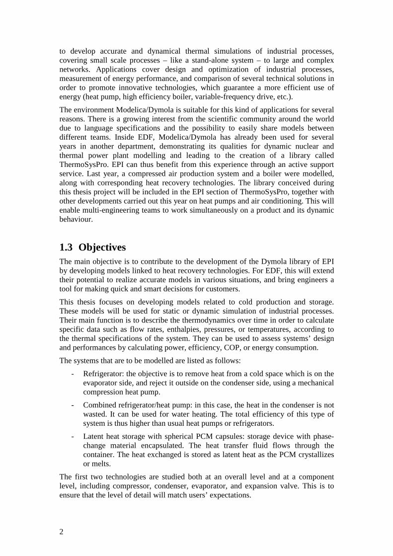
to develop accurate and dynamical thermal simulations of industrial processes, covering small scale processes – like a stand-alone system – to large and complex networks. Applications cover design and optimization of industrial processes, measurement of energy performance, and comparison of several technical solutions in order to promote innovative technologies, which guarantee a more efficient use of energy (heat pump, high efficiency boiler, variable-frequency drive, etc.).

The environment Modelica/Dymola is suitable for this kind of applications for several reasons. There is a growing interest from the scientific community around the world due to language specifications and the possibility to easily share models between different teams. Inside EDF, Modelica/Dymola has already been used for several years in another department, demonstrating its qualities for dynamic nuclear and thermal power plant modelling and leading to the creation of a library called ThermoSysPro. EPI can thus benefit from this experience through an active support service. Last year, a compressed air production system and a boiler were modelled, along with corresponding heat recovery technologies. The library conceived during this thesis project will be included in the EPI section of ThermoSysPro, together with other developments carried out this year on heat pumps and air conditioning. This will enable multi-engineering teams to work simultaneously on a product and its dynamic behaviour.

1.3 Objectives The main objective is to contribute to the development of the Dymola library of EPI by developing models linked to heat recovery technologies. For EDF, this will extend their potential to realize accurate models in various situations, and bring engineers a tool for making quick and smart decisions for customers.

This thesis focuses on developing models related to cold production and storage. These models will be used for static or dynamic simulation of industrial processes. Their main function is to describe the thermodynamics over time in order to calculate specific data such as flow rates, enthalpies, pressures, or temperatures, according to the thermal specifications of the system. They can be used to assess systems’ design and performances by calculating power, efficiency, COP, or energy consumption.

The systems that are to be modelled are listed as follows:

- Refrigerator: the objective is to remove heat from a cold space which is on the evaporator side, and reject it outside on the condenser side, using a mechanical compression heat pump.

- Combined refrigerator/heat pump: in this case, the heat in the condenser is not wasted. It can be used for water heating. The total efficiency of this type of system is thus higher than usual heat pumps or refrigerators.

- Latent heat storage with spherical PCM capsules: storage device with phase-change material encapsulated. The heat transfer fluid flows through the container. The heat exchanged is stored as latent heat as the PCM crystallizes or melts.

The first two technologies are studied both at an overall level and at a component level, including compressor, condenser, evaporator, and expansion valve. This is to ensure that the level of detail will match users’ expectations.

3

The library developed has to be independent (i.e. do not depend on other libraries) in order to facilitate its future integration and diffusion at EDF, while following pre-established development rules to make the new models consistent with the other ones developed at EDF. To guarantee the ease of use of the models for future users, documentation will be formulated and supplied together with the models.

1.4 Methodology The initial phase of the thesis relied on an extensive literature review of the environment Modelica/Dymola in order to learn the basics of the programming language. The purpose was to get a comprehensive and efficient use of the language, in order to take advantage of its intrinsic qualities and to be aware of all its constraints. The project aims at developing models that are user-friendly, i.e. accessible and quick to configure.

The working method for developing each model can be summarized into the following steps:

1. Pre-literature review

To begin with, a short technical review is made in order to understand properly how the system is working.

2. Choice of the modelling level of details

A specific technology can be studied at an overall level (i.e. treated as a “black box”), at a component level (i.e. including sub-systems like compressor, condenser, evaporator), or even further in details (e.g. description of heat exchanger geometry). This determines the type of parameters and equations required for the model.

3. Selection of the values to calculate

A model can have different purposes: it can calculate basic thermodynamic values based on inputs or outputs (flow rate, temperature, pressure) as well as various ratios, performance-related values, or anything which is of interest for the user. This has to be determined in order to make a model that will meet all or at least most of the expectations anyone could have with a dynamic simulation.

4. In-depth literature review

Once the model has been defined, a detailed literature review is conducted, more focused on the physics and the mathematical description of the system. Each system has different thermodynamic properties corresponding to their characteristics and the type of fluids used. These properties, as well as the equations associated with them, have to be studied since they constitute the heart of the model. Equations usually describe thermodynamic equilibrium, heat balance, or simply how state variables such as pressure and temperature evolve across the system.

5. Model programming

Gathering all the previously collected data, it is now possible to start the actual programming under Modelica/Dymola. The programming is done step-by-step, starting from a very basic model and ending with a much more detailed one (including more variables, parameters or equations, or a simpler interface). This is to ensure that any cause of trouble can be easily detected and to clearly see how simulations evolve in function of the model complexity.

4

6. Robustness testing

When the model is set-up, its accuracy has to be verified through a series of tests. These tests range from simple test cases (e.g. the system alone) to complex and closed-circuit cases where other systems are included, to reproduce a real industrial case. A comparative analysis with experimental data is also conducted to validate the models or reveal the need for improvements. This data is obtained from projects in which EDF is involved and where measurements or calculations have been done. This will ensure the quality of the model and its capacity to be implemented in more complex cases.

5

2 Presentation of Modelica and Dymola 2.1 The Modelica language 2.1.1 General introduction The Modelica language has been developed since 1996 by the Modelica Association, a non-profit organization based in Linköping, Sweden, which gathers members from Europe and the US.

Modelica is a freely available, object-oriented language for modelling of large and complex systems. The program language is mainly used for computer simulation of dynamic systems where behaviour evolves as a function of time. It has been designed to deal with multi-domain modelling; this means that several aspects of physics can be treated in the same model, for instance, an automotive application involving mechanical, electrical, hydraulic and control subsystems. All these objects can be described and connected.

Modelica differs from other languages because it is based on equations instead of assignment statements. This means that a model describes the physical equations governing a system and not the algorithm routine to solve them. Variables are not defined as inputs or outputs since their role can be reversed. This allows acausal modelling that gives better reuse of classes since equations do not specify a certain data flow direction.

Models in Modelica are mathematically described by differential, algebraic and/or discrete equations. A Modelica tool will have enough information to decide which variables need to be solved. The language is designed such that available, specialized algorithms can be utilized to enable efficient handling of large models having more than 100,000 equations.

As mentioned before, Modelica is designed to be domain neutral and can thus be used in a wide variety of applications, such as automotive industry or energy systems.

In parallel of its work, the Modelica Association develops and distributes for free the Modelica Standard Library. It is a reference library which is broadly used as a base for any model, since it includes typical classes1.

2.1.2 Basic programming concepts Modelica programs are built from classes that are usually called models. As it is an object-oriented language, it is possible to create any number of objects from a class definition, making instances of that class. Classes, or models, are always gathered in a package, which can be considered as the equivalent of a folder in a computer operating system. Packages are thus used to organize models hierarchically. Finally, all the models and packages add up to constitute a library.

1 The fundamental structuring unit of modelling in Modelica is the class. Classes provide the structure for objects, also known as instances. Classes can contain equations which provide the basis for the executable code that is used for computation in Modelica. All data objects in Modelica are instantiated from classes, including the basic data types (Real, Integer, String, Boolean) which are built-in classes.

6

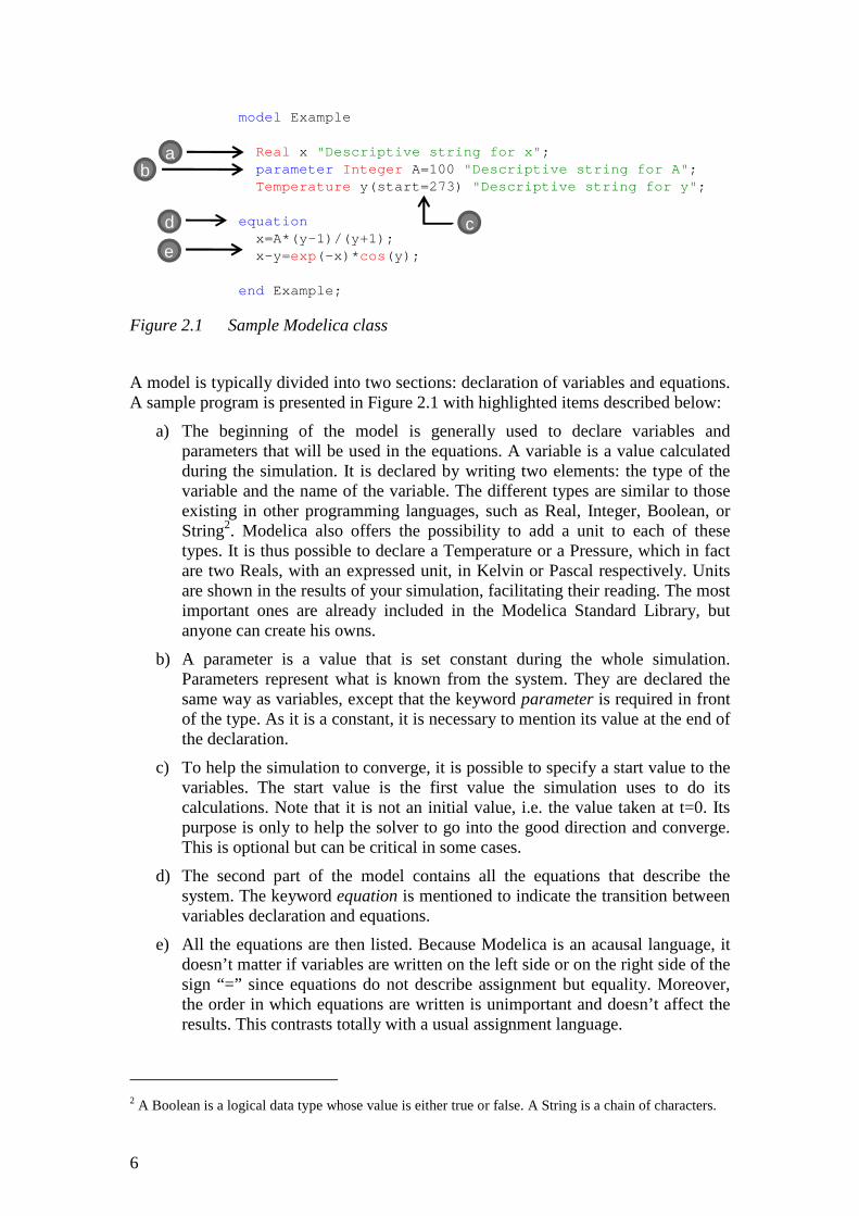
Figure 2.1 Sample Modelica class

A model is typically divided into two sections: declaration of variables and equations. A sample program is presented in Figure 2.1 with highlighted items described below:

a) The beginning of the model is generally used to declare variables and parameters that will be used in the equations. A variable is a value calculated during the simulation. It is declared by writing two elements: the type of the variable and the name of the variable. The different types are similar to those existing in other programming languages, such as Real, Integer, Boolean, or String2. Modelica also offers the possibility to add a unit to each of these types. It is thus possible to declare a Temperature or a Pressure, which in fact are two Reals, with an expressed unit, in Kelvin or Pascal respectively. Units are shown in the results of your simulation, facilitating their reading. The most important ones are already included in the Modelica Standard Library, but anyone can create his owns.

b) A parameter is a value that is set constant during the whole simulation. Parameters represent what is known from the system. They are declared the same way as variables, except that the keyword parameter is required in front of the type. As it is a constant, it is necessary to mention its value at the end of the declaration.

c) To help the simulation to converge, it is possible to specify a start value to the variables. The start value is the first value the simulation uses to do its calculations. Note that it is not an initial value, i.e. the value taken at t=0. Its purpose is only to help the solver to go into the good direction and converge. This is optional but can be critical in some cases.

d) The second part of the model contains all the equations that describe the system. The keyword equation is mentioned to indicate the transition between variables declaration and equations.

e) All the equations are then listed. Because Modelica is an acausal language, it doesn’t matter if variables are written on the left side or on the right side of the sign “=” since equations do not describe assignment but equality. Moreover, the order in which equations are written is unimportant and doesn’t affect the results. This contrasts totally with a usual assignment language.

2 A Boolean is a logical data type whose value is either true or false. A String is a chain of characters.

model Example

Real x "Descriptive string for x";parameter Integer A=100 "Descriptive string for A";Temperature y(start=273) "Descriptive string for y";

equationx=A*(y-1)/(y+1);x-y=exp(-x)*cos(y);

end Example;

ab

cd

e

7

Although Modelica relies on equations, it is still possible to write classic assignment algorithms by mentioning the keyword algorithm in the model. Algorithms are not preferable compared to the flexibility given by the equations and it would be senseless to only use algorithms instead of equations. However, they are essential in some situations and especially when it comes to functions. A function is a class that contains a sequence of instructions. They can be called in equation-based models to calculate variables. For instance, they can be used to get thermodynamic properties of fluids from temperature and pressure, as described in Section 3.4.3.

Comments and text that is not read during the simulation have different forms. A string description of a variable is written in quotation marks "". A general comment can be written after a double-slash // or between /* and */. Finally, annotations are intended to store extra information about a model, such as graphics, documentation, or the graphical user interface of the parameters dialog (see Section 3.3.1).

A last important point about Modelica language is that simulations can be done only if the number of equations in the model is equal to the number of variables (zero degree of freedom). Otherwise, an error is returned.

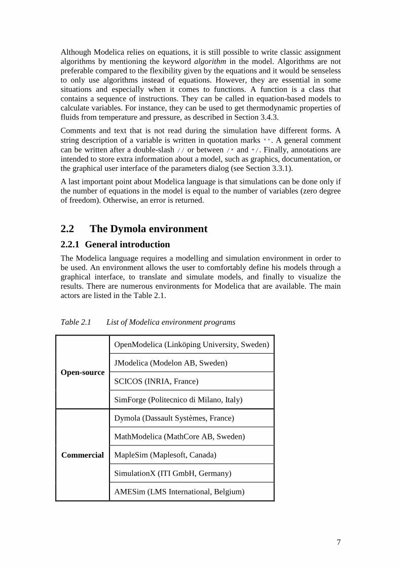
2.2 The Dymola environment 2.2.1 General introduction The Modelica language requires a modelling and simulation environment in order to be used. An environment allows the user to comfortably define his models through a graphical interface, to translate and simulate models, and finally to visualize the results. There are numerous environments for Modelica that are available. The main actors are listed in the Table 2.1.

Table 2.1 List of Modelica environment programs

Open-source

OpenModelica (Linköping University, Sweden)

JModelica (Modelon AB, Sweden)

SCICOS (INRIA, France)

SimForge (Politecnico di Milano, Italy)

Commercial

Dymola (Dassault Systèmes, France)

MathModelica (MathCore AB, Sweden)

MapleSim (Maplesoft, Canada)

SimulationX (ITI GmbH, Germany)

AMESim (LMS International, Belgium)

8

The most advanced and well-known program is Dymola (Dynamic Modeling Laboratory). It is the one EDF has chosen for its research works, since it is an efficient and robust tool that has been tested and approved by several companies and universities.

Dymola is a commercial environment that has been developed since 1992 by the Swedish company Dynasim AB, acquired by the French company Dassault Systèmes in 2006 (Cellier, 2005). It can be interfaced with other programs like CATIA, Simulink, or Excel. This partly explains why it is increasingly used by industries such as Ford (automotive), Toyota (automotive), Saab (aircraft), Tetra Pak (food packaging), Ceres Power (heat and power), or Solvina (energy system design) (Dassault Systèmes, 2010).

The version used during the thesis was Dymola 7.4. In order to make simulations, a C++ compiler has to be installed, like Visual Studio.

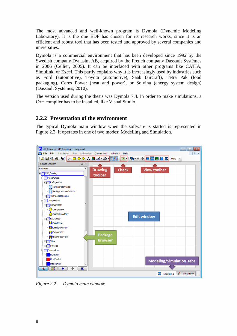
2.2.2 Presentation of the environment The typical Dymola main window when the software is started is represented in Figure 2.2. It operates in one of two modes: Modelling and Simulation.

Figure 2.2 Dymola main window

9

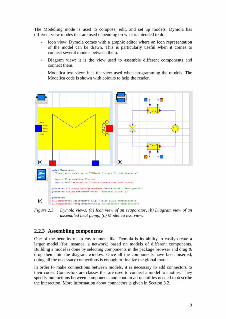
The Modelling mode is used to compose, edit, and set up models. Dymola has different view modes that are used depending on what is intended to do:

- Icon view: Dymola comes with a graphic editor where an icon representation of the model can be drawn. This is particularly useful when it comes to connect several models between them.

- Diagram view: it is the view used to assemble different components and connect them.

- Modelica text view: it is the view used when programming the models. The Modelica code is shown with colours to help the reader.

Figure 2.3 Dymola views: (a) Icon view of an evaporator, (b) Diagram view of an assembled heat pump, (c) Modelica text view.

2.2.3 Assembling components One of the benefits of an environment like Dymola is its ability to easily create a larger model (for instance, a network) based on models of different components. Building a model is done by selecting components in the package browser and drag & drop them into the diagram window. Once all the components have been inserted, doing all the necessary connections is enough to finalize the global model.

In order to make connections between models, it is necessary to add connectors to their codes. Connectors are classes that are used to connect a model to another. They specify interactions between components and contain all quantities needed to describe the interaction. More information about connectors is given in Section 3.2.

(a) (b)

(c)

10

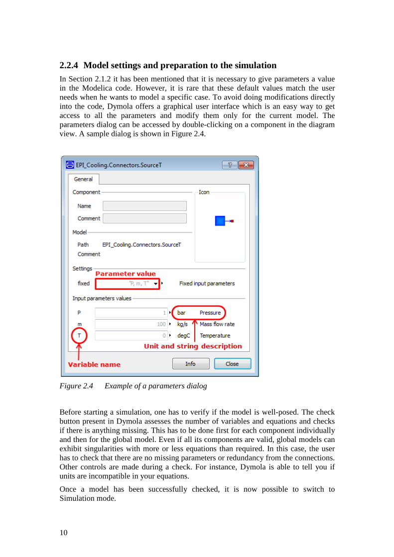
2.2.4 Model settings and preparation to the simulation In Section 2.1.2 it has been mentioned that it is necessary to give parameters a value in the Modelica code. However, it is rare that these default values match the user needs when he wants to model a specific case. To avoid doing modifications directly into the code, Dymola offers a graphical user interface which is an easy way to get access to all the parameters and modify them only for the current model. The parameters dialog can be accessed by double-clicking on a component in the diagram view. A sample dialog is shown in Figure 2.4.

Figure 2.4 Example of a parameters dialog

Before starting a simulation, one has to verify if the model is well-posed. The check button present in Dymola assesses the number of variables and equations and checks if there is anything missing. This has to be done first for each component individually and then for the global model. Even if all its components are valid, global models can exhibit singularities with more or less equations than required. In this case, the user has to check that there are no missing parameters or redundancy from the connections. Other controls are made during a check. For instance, Dymola is able to tell you if units are incompatible in your equations.

Once a model has been successfully checked, it is now possible to switch to Simulation mode.

11

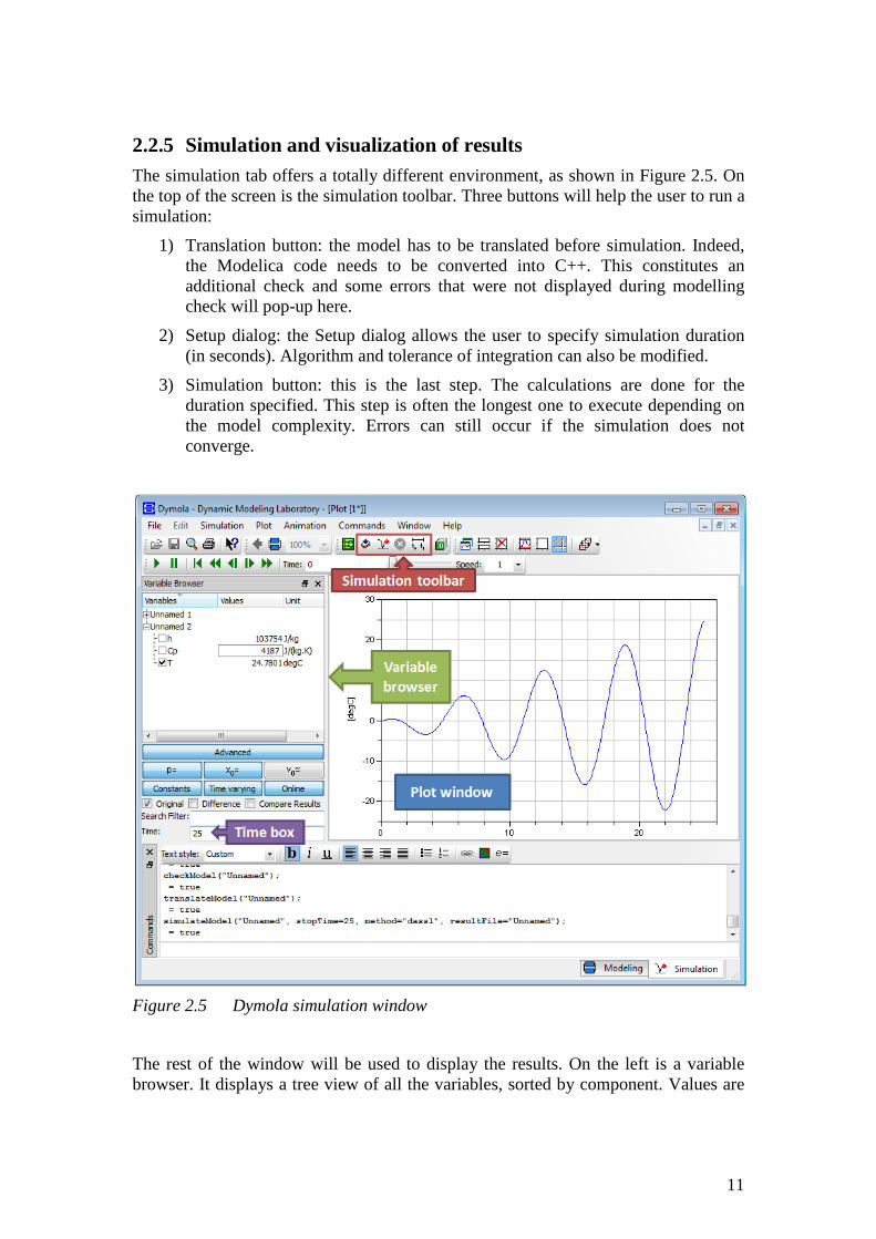
2.2.5 Simulation and visualization of results The simulation tab offers a totally different environment, as shown in Figure 2.5. On the top of the screen is the simulation toolbar. Three buttons will help the user to run a simulation:

1) Translation button: the model has to be translated before simulation. Indeed, the Modelica code needs to be converted into C++. This constitutes an additional check and some errors that were not displayed during modelling check will pop-up here.

2) Setup dialog: the Setup dialog allows the user to specify simulation duration (in seconds). Algorithm and tolerance of integration can also be modified.

3) Simulation button: this is the last step. The calculations are done for the duration specified. This step is often the longest one to execute depending on the model complexity. Errors can still occur if the simulation does not converge.

Figure 2.5 Dymola simulation window

The rest of the window will be used to display the results. On the left is a variable browser. It displays a tree view of all the variables, sorted by component. Values are

12

given for the time specified in the corresponding box, along with their unit and description.

It is possible to plot any variable versus time, to get a better idea of how the model variables evolve. Plots are customizable with colours, titles, legend, and other appearance parameters.

13

3 General principles and models 3.1 Development rules The Modelica/Dymola environment is suitable for modelling of various kinds of physical systems. The models and libraries developed are truly reusable if they are well-programmed. It is important to state common rules and then verify that they are respected in order to ensure compatibility. Advices and recommendations for conception have been made inside EDF R&D to facilitate models and results readability (Bouskela, 2003). This is also to simplify the sharing and distribution of the libraries when they will be integrated in larger projects. Eventually, models have to be adjusted so as to minimize their adherence to the commercial tool Dymola so that they can be used in other programs like OpenModelica. Below are given some important rules that have been applied during the thesis:

- Unrestricted: models do not impose any hypothesis or unwanted physical limitation that is not part of their concept. The value of a specific heat capacity, for instance, is not directly written in the equations, but rather in a parameter, even if the fluid used is supposed to stay the same. If the system is meshed, the precision can be freely chosen.

- Easy to understand: models are clearly structured, with different sections. All variables are described and equations commented. A naming convention is established to allow quick identification of variable type.

- Easy to define: a great attention is given to the layout of parameters dialogs, with sections, tabs, check boxes or radio buttons, so that the user won’t get lost in the list of parameters.

- Exemplified: each component is given with an example model to allow the user to quickly test it and see what variables are expected at the inlet and the outlet (see Section 3.3).

- Easy to interpret: useful variables should be shown in the results whereas others should be hidden (via the keyword protected).

In the rest of this chapter are presented models that are reused for the development of all the systems described in Chapters 4, 5 and 6. These models are regrouped into connectors, sources and sinks, and thermodynamic properties of fluids. Several where already defined in the library ThermoSysPro, but most of them seemed outdated or unsuitable for the models to be developed. There was also an expressed will to have something simple, complete and universal for all the future needs.

Some of these models are presented in Appendix 1.

3.2 Connectors Complex systems usually consist of large numbers of connected components. To achieve these connections, connectors are used. They are classes that specify variables transmitted through a connection. They have to be directly included in a component code since they represent its inlets and/or outlets. For instance, a pipe has two connectors: one inlet and one outlet. A classic heat exchanger has four: two inlets and two outlets. The variables can be reals, integers, logical, or physical.

14

The project conducted during the thesis is related to thermal and energy systems. Three appropriate variables have been selected considering that systems are always working with fluids. These variables are pressure P, mass flow rate m, and specific enthalpy h. These properties are enough to fully describe the state of a fluid. Supplementary connectors with temperature instead of enthalpy have also been created. Temperature cannot always be used because they are problematic during phase transition. However, for industrial applications, it is more common to know the temperature of your fluids instead of their enthalpy. The models with temperature connectors will be stressed in the thesis. All the units used are SI.

The Modelica code of a connector consists only of the variables declarations. There are no equations in a connector. To help users to make connections properly, two additional logical variables have been included. They verify that an inlet is not connected to another inlet and the same for an outlet. Thus, two different connectors have been modelled: FluidInlet and FluidOutlet. Their code is exactly the same except for the value taken by the two Booleans.

When a connection is created in the diagram view of Dymola (see Section 2.2.3), an equation is added to the model:

connect(component1.connector1, component2.connector2);

This equation means that all the variables in the connector1 of component1 are equal to the ones in the connector2 of component2. It means that all the variables transmitted through a connection remain constants.

In order to transmit values, equations inside each component are needed, which assigns values to the connectors’ variables. Connections to connectors should impose the right amount of constraints. For instance, the pressure P must not be calculated at both sides of the connection, otherwise the equality between connectors’ variables cannot be guaranteed. One side should get the value from a component calculation whilst the other side just receives the value from the connection. This remark is especially relevant when it comes to closed-circuit models such as the refrigeration cycles studied within this work.

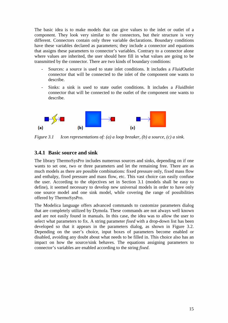
3.3 Loop breakers There is indeed a special problem regarding equation systems resulting from models with a loop structure. If a variable is spread from a component in both directions (its input and its output), there will be a location in the system with an overconstrained connection (the same variable coming from both sides). To overcome this, loop breakers have been created. There are small classes that have to be put in the middle of the connection where this problem appears. It specifies which variables must not be transmitted through it, among the variables of the connectors. This will delete the redundant equations in the connection, making the closed-circuit model working.

3.4 Sources and sinks When making a model or testing a component, it is particularly helpful to make use of boundary conditions. Thus, it is not necessary to build a complete network to check if the components developed are working. Classes for boundary conditions will represent the extremities of an open-circuit model.

15

The basic idea is to make models that can give values to the inlet or outlet of a component. They look very similar to the connectors, but their structure is very different. Connectors contain only three variable declarations. Boundary conditions have these variables declared as parameters; they include a connector and equations that assigns these parameters to connector’s variables. Contrary to a connector alone where values are inherited, the user should here fill in what values are going to be transmitted by the connector. There are two kinds of boundary conditions:

- Sources: a source is used to state inlet conditions. It includes a FluidOutlet connector that will be connected to the inlet of the component one wants to describe.

- Sinks: a sink is used to state outlet conditions. It includes a FluidInlet connector that will be connected to the outlet of the component one wants to describe.

Figure 3.1 Icon representations of: (a) a loop breaker, (b) a source, (c) a sink.

3.4.1 Basic source and sink The library ThermoSysPro includes numerous sources and sinks, depending on if one wants to set one, two or three parameters and let the remaining free. There are as much models as there are possible combinations: fixed pressure only, fixed mass flow and enthalpy, fixed pressure and mass flow, etc. This vast choice can easily confuse the user. According to the objectives set in Section 3.1 (models shall be easy to define), it seemed necessary to develop new universal models in order to have only one source model and one sink model, while covering the range of possibilities offered by ThermoSysPro.

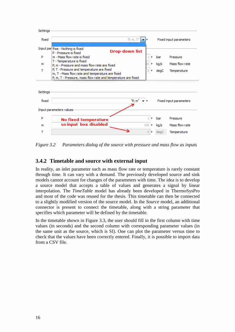
The Modelica language offers advanced commands to customize parameters dialog that are completely utilized by Dymola. These commands are not always well known and are not easily found in manuals. In this case, the idea was to allow the user to select what parameters to fix. A string parameter fixed with a drop-down list has been developed so that it appears in the parameters dialog, as shown in Figure 3.2. Depending on the user’s choice, input boxes of parameters become enabled or disabled, avoiding any doubt about what needs to be filled in. This choice also has an impact on how the source/sink behaves. The equations assigning parameters to connector’s variables are enabled according to the string fixed.

16

Figure 3.2 Parameters dialog of the source with pressure and mass flow as inputs

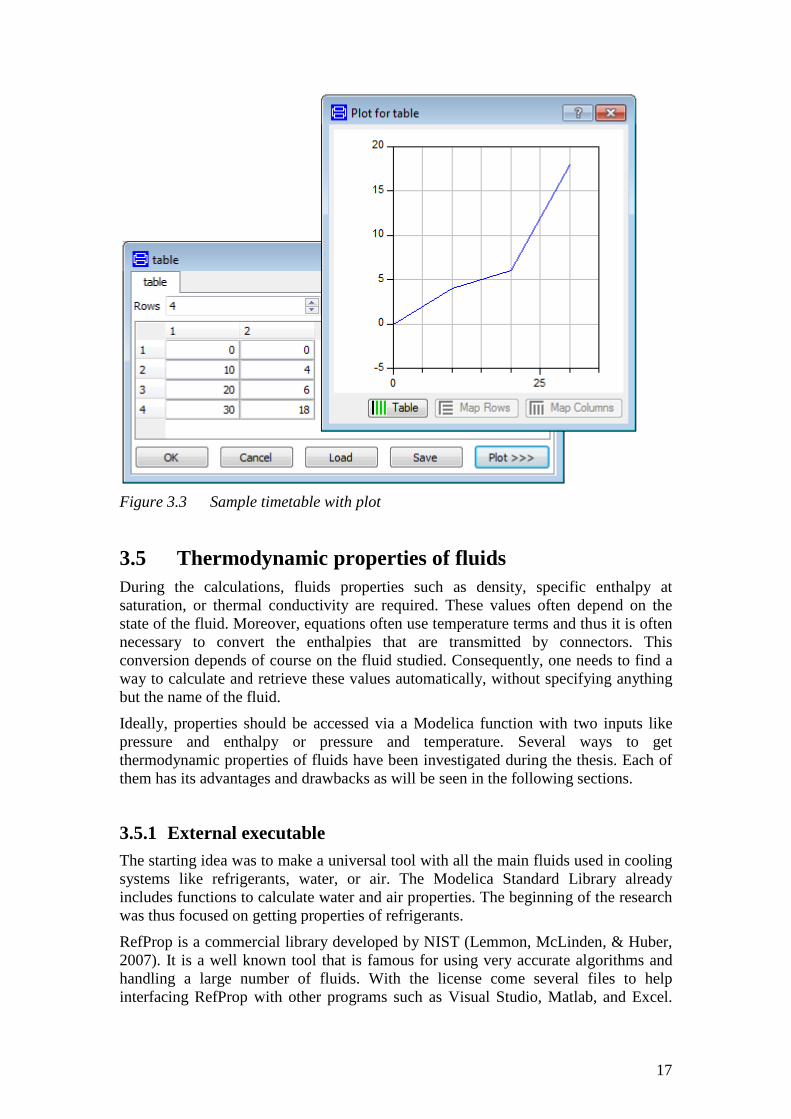
3.4.2 Timetable and source with external input In reality, an inlet parameter such as mass flow rate or temperature is rarely constant through time. It can vary with a demand. The previously developed source and sink models cannot account for changes of the parameters with time. The idea is to develop a source model that accepts a table of values and generates a signal by linear interpolation. The TimeTable model has already been developed in ThermoSysPro and most of the code was reused for the thesis. This timetable can then be connected to a slightly modified version of the source model. In the Source model, an additional connector is present to connect the timetable, along with a string parameter that specifies which parameter will be defined by the timetable.

In the timetable shown in Figure 3.3, the user should fill in the first column with time values (in seconds) and the second column with corresponding parameter values (in the same unit as the source, which is SI). One can plot the parameter versus time to check that the values have been correctly entered. Finally, it is possible to import data from a CSV file.

17

Figure 3.3 Sample timetable with plot

3.5 Thermodynamic properties of fluids During the calculations, fluids properties such as density, specific enthalpy at saturation, or thermal conductivity are required. These values often depend on the state of the fluid. Moreover, equations often use temperature terms and thus it is often necessary to convert the enthalpies that are transmitted by connectors. This conversion depends of course on the fluid studied. Consequently, one needs to find a way to calculate and retrieve these values automatically, without specifying anything but the name of the fluid.

Ideally, properties should be accessed via a Modelica function with two inputs like pressure and enthalpy or pressure and temperature. Several ways to get thermodynamic properties of fluids have been investigated during the thesis. Each of them has its advantages and drawbacks as will be seen in the following sections.

3.5.1 External executable The starting idea was to make a universal tool with all the main fluids used in cooling systems like refrigerants, water, or air. The Modelica Standard Library already includes functions to calculate water and air properties. The beginning of the research was thus focused on getting properties of refrigerants.

RefProp is a commercial library developed by NIST (Lemmon, McLinden, & Huber, 2007). It is a well known tool that is famous for using very accurate algorithms and handling a large number of fluids. With the license come several files to help interfacing RefProp with other programs such as Visual Studio, Matlab, and Excel.

18

There is, however, no official interface for Modelica, making its implementation difficult.

In 2010, Assaf from the CEP Mines ParisTech, developed in collaboration with EDF a small program called Refbib (Assaf, 2010). Refbib is based on the RefProp library and requires all the fluid files that come with it. The purpose of Refbib is to access RefProp files from any program, by executing an external executable. This executable reads a .txt file containing the input parameters: name of the fluid, type of the two input variables, and their respecting values. Refbib supports 4 combinations for the input variables: pressure and enthalpy, pressure and vapour fraction, pressure and entropy, and temperature and vapour fraction. From this information, it is able to calculate thermodynamic properties of fluids such as temperature, enthalpy, entropy, density, specific heat capacity and thermal conductivity, with their respecting saturated liquid and vapour values. After its execution, another .txt file is created with the results. No graphical user interface is associated with the program. When it is executed, it just calculates the inherent values in background and creates the output file.

In order to use this program in Modelica, a function has been made to automatically create the input .txt file and read the output file by assigning each result to a variable. A simple function call like the one below creates a record where all the resulting values are stored:

record=Refbib("fluid name", "P", "H", pressure, enthalpy);

Values are then referenced as record.T, record.h, record.Cp, etc.

This solution has been tested and approved for some case tests. However, some of the values obtained were erroneous, like enthalpies or densities with an exponent 14. Moreover, it often happens that the simulation is not able to converge using this solution. Another default is that Refbib cannot handle pressure and temperature as inputs. This option is very important for an optimal development of the models, as will be described in Chapter 4. Finally, since Modelica does iterative calculations, the simulation has to repeatedly call the program, increasing the time required to get the good result. Compared to the alternative solutions described next, a simulation can take 100 to 1000 times longer (about 20 seconds for a simple refrigerator). These critical issues forced the complete abandon of the Refbib solution.

3.5.2 Dynamic library Since RefProp offers many advantages, it was decided to continue finding another solution that takes benefits of a RefProp interface. After some research online and in the scientific literature, it was observed that no free Modelica model has been developed in this way. Only a commercial library named TIL and developed by TLK-Thermo GmbH includes a RefProp interface (TLK-Thermo GmbH, 2009). The TIL library is a Modelica library specialized in the advanced modelling of thermodynamic systems. The next idea was to retrieve the classes doing the interface and put them in the developed EPI library, in order to use them independently from the rest of the TIL library.

TIL uses a Dynamic Link Library (DLL) file, TILMedia204.dll, and a C file in order to access to the RefProp database. Modelica has the ability to call external functions in files wrote in C. The use of the TILMedia library is based on calling these functions

19

within Modelica files. These functions access to the DLL file, which will read the RefProp database.

Getting fluid properties into a model is fairly simple. Basically, a refrigerant is declared as an object, with a parameter specifying what variable couple has been chosen as input: pressure and enthalpy, pressure and entropy, pressure and temperature, or density and temperature. The refrigerant object contains variables representing all its thermodynamic properties. By assigning a value to the two input variables, the properties are calculated and it is possible to access any of the other variables of the refrigerant object according to the following:

Refrigerant ref(refrigerantName, inputChoice=ph); //Declaration equation ref.p=Pf; //Assigning first input value ref.h=hf; //Assigning second input value Tf=ref.T; //Retrieving corresponding temperature

Compared to Refbib, this solution is a lot more reliable. All values are correct and no mistakes were detected during tests. The calculation time is excellent with instantaneous simulations. It perfectly handles the 90 fluids included in RefProp as well as 55 mixtures. This solution can be used for accurate models with refrigerants. However, as it comes from a commercial library, it is important to highlight that it is necessary to buy a license in order to use it. This prevents a possible distribution of the EPI library, restricting its use to internal R&D research. Note that the TILMedia library seems to fail when used in combination with the Modelica Standard library’s properties functions. It is thus better to calculate water and air properties with TILMedia when it is used for refrigerants.

3.5.3 Polynomial functions Despite its numerous advantages, using RefProp in Modelica simulations is not perfect yet. The last alternative is to ignore RefProp and calculate fluid properties through Modelica functions directly coded in the library. Air and water are already included in the Modelica Standard Library. However, there are no models for refrigerants. It was necessary to find mathematical representations of these fluids. The Massey University, New Zealand, published polynomial curve-fit equations for refrigerant thermodynamic properties (Cleland, 1992). These equations have been translated into Modelica functions. They use third order polynomials that are function of temperature. Once all the functions coded, it is possible to calculate saturation pressure, saturation temperature, enthalpy of liquid and vapour phase, latent heat, and enthalpy change in isentropic compression. For instance, saturation pressure can be calculated from saturation temperature as follows:

Psat=Psat(Tsat);

The range of applicability is -40°C ≤ Tsat ≤ 70°C.

Modelica functions can be used as inverse functions. It means that it is possible to calculate an input of a function instead of its output, by writing exactly the same equation as if the output was the unknown. This is again due to the acausality of the Modelica language. Therefore, one can get the saturation temperature from the saturation pressure with the same equation written above.

20

The polynomial solution is very fast and no latency due to properties calculations has been observed. Moreover, 100% of test simulations have been able to converge, even the ones where TILMedia failed. It can thus be very useful as a back-up solution.

However, this solution has its disadvantages. First, it remains less accurate than RefProp. Cleland claims in his article that the predicted properties generally agree with the source data to within about ±0.4%. This value was indeed observed during tests. This has to be weighted considering the category of simulations conducted, and accepted as a moderate margin of error. Secondly, it is a far less complete solution, since most of the fluid properties such as density and heat capacities are not calculated. It also takes much more time to integrate several fluids since all the code has to be entered manually, not taking advantage of a pre-made database. During the thesis, only R134a have been modelled by polynomial equations.

21

4 Refrigerator modelling 4.1 Presentation of the technology Industries such as food industries often require the use of cold fluids in their networks, to satisfy their needs in cooling or preservation of goods at low temperatures. A refrigerator offers an efficient solution to produce cold.

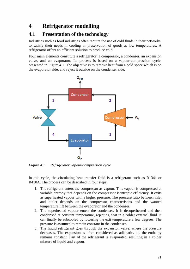
Four main elements constitute a refrigerator: a compressor, a condenser, an expansion valve, and an evaporator. Its process is based on a vapour-compression cycle, presented in Figure 4.1. The objective is to remove heat from a cold space which is on the evaporator side, and reject it outside on the condenser side.

Figure 4.1 Refrigerator vapour-compression cycle

In this cycle, the circulating heat transfer fluid is a refrigerant such as R134a or R410A. The process can be described in four steps:

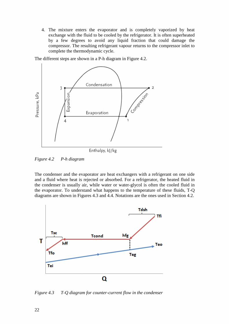
1. The refrigerant enters the compressor as vapour. This vapour is compressed at variable entropy that depends on the compressor isentropic efficiency. It exits as superheated vapour with a higher pressure. The pressure ratio between inlet and outlet depends on the compressor characteristics and the wanted temperature lift between the evaporator and the condenser.

2. The superheated vapour enters the condenser. It is desuperheated and then condensed at constant temperature, rejecting heat in a colder external fluid. It can finally be subcooled by lowering the exit temperature a few degrees. The pressure is assumed to remain constant in the condenser.

3. The liquid refrigerant goes through the expansion valve, where the pressure decreases. The expansion is often considered as adiabatic, i.e. the enthalpy remains constant. Part of the refrigerant is evaporated, resulting in a colder mixture of liquid and vapour.

22

4. The mixture enters the evaporator and is completely vaporized exchange with the fluid to be cooled by theby a few degrees to avoid any liquid fraction that could damage the compressor. The resulting refrigerant vapour returns to the compressor inlet to complete the thermodynamic cycle.

The different steps are shown

Figure 4.2 P-h diagram

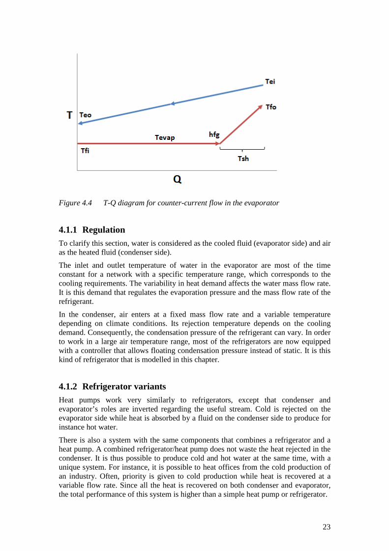
The condenser and the evaporator are heat exchangers with and a fluid where heat is rejected or the condenser is usually air, while water or waterthe evaporator. To understand what happens to the temperature of these fluids, Tdiagrams are shown in Figure

Figure 4.3 T-Q diagram for counter

The mixture enters the evaporator and is completely vaporized exchange with the fluid to be cooled by the refrigerator. It is often superheated by a few degrees to avoid any liquid fraction that could damage the compressor. The resulting refrigerant vapour returns to the compressor inlet to complete the thermodynamic cycle.

shown in a P-h diagram in Figure 4.2.

diagram

The condenser and the evaporator are heat exchangers with a refrigerant on one side fluid where heat is rejected or absorbed. For a refrigerator, the

the condenser is usually air, while water or water-glycol is often the cooled fluid in To understand what happens to the temperature of these fluids, T

diagrams are shown in Figures 4.3 and 4.4. Notations are the ones used in Se

Q diagram for counter-current flow in the condenser

The mixture enters the evaporator and is completely vaporized by heat refrigerator. It is often superheated

by a few degrees to avoid any liquid fraction that could damage the compressor. The resulting refrigerant vapour returns to the compressor inlet to

refrigerant on one side For a refrigerator, the heated fluid in

glycol is often the cooled fluid in To understand what happens to the temperature of these fluids, T-Q

Notations are the ones used in Section 4.2.

23

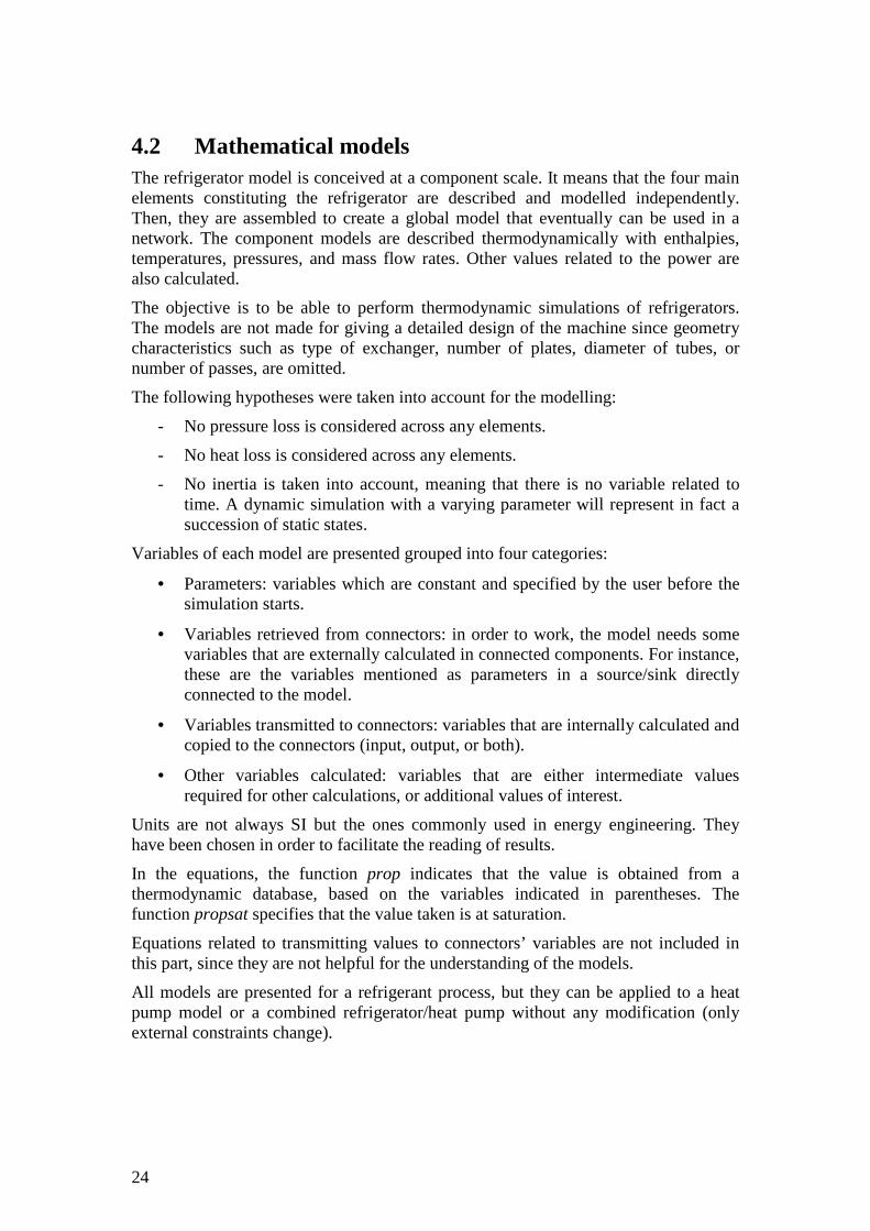
Figure 4.4 T-Q diagram for counter-current flow in the evaporator

4.1.1 Regulation To clarify this section, water is considered as the cooled fluid (evaporator side) and air as the heated fluid (condenser side).

The inlet and outlet temperature of water in the evaporator are most of the time constant for a network with a specific temperature range, which corresponds to the cooling requirements. The variability in heat demand affects the water mass flow rate. It is this demand that regulates the evaporation pressure and the mass flow rate of the refrigerant.

In the condenser, air enters at a fixed mass flow rate and a variable temperature depending on climate conditions. Its rejection temperature depends on the cooling demand. Consequently, the condensation pressure of the refrigerant can vary. In order to work in a large air temperature range, most of the refrigerators are now equipped with a controller that allows floating condensation pressure instead of static. It is this kind of refrigerator that is modelled in this chapter.

4.1.2 Refrigerator variants Heat pumps work very similarly to refrigerators, except that condenser and evaporator’s roles are inverted regarding the useful stream. Cold is rejected on the evaporator side while heat is absorbed by a fluid on the condenser side to produce for instance hot water.

There is also a system with the same components that combines a refrigerator and a heat pump. A combined refrigerator/heat pump does not waste the heat rejected in the condenser. It is thus possible to produce cold and hot water at the same time, with a unique system. For instance, it is possible to heat offices from the cold production of an industry. Often, priority is given to cold production while heat is recovered at a variable flow rate. Since all the heat is recovered on both condenser and evaporator, the total performance of this system is higher than a simple heat pump or refrigerator.

24

4.2 Mathematical models The refrigerator model is conceived at a component scale. It means that the four main elements constituting the refrigerator are described and modelled independently. Then, they are assembled to create a global model that eventually can be used in a network. The component models are described thermodynamically with enthalpies, temperatures, pressures, and mass flow rates. Other values related to the power are also calculated.

The objective is to be able to perform thermodynamic simulations of refrigerators. The models are not made for giving a detailed design of the machine since geometry characteristics such as type of exchanger, number of plates, diameter of tubes, or number of passes, are omitted.

The following hypotheses were taken into account for the modelling:

- No pressure loss is considered across any elements.

- No heat loss is considered across any elements.

- No inertia is taken into account, meaning that there is no variable related to time. A dynamic simulation with a varying parameter will represent in fact a succession of static states.

Variables of each model are presented grouped into four categories:

• Parameters: variables which are constant and specified by the user before the simulation starts.

• Variables retrieved from connectors: in order to work, the model needs some variables that are externally calculated in connected components. For instance, these are the variables mentioned as parameters in a source/sink directly connected to the model.

• Variables transmitted to connectors: variables that are internally calculated and copied to the connectors (input, output, or both).

• Other variables calculated: variables that are either intermediate values required for other calculations, or additional values of interest.

Units are not always SI but the ones commonly used in energy engineering. They have been chosen in order to facilitate the reading of results.

In the equations, the function prop indicates that the value is obtained from a thermodynamic database, based on the variables indicated in parentheses. The function propsat specifies that the value taken is at saturation.

Equations related to transmitting values to connectors’ variables are not included in this part, since they are not helpful for the understanding of the models.

All models are presented for a refrigerant process, but they can be applied to a heat pump model or a combined refrigerator/heat pump without any modification (only external constraints change).

25

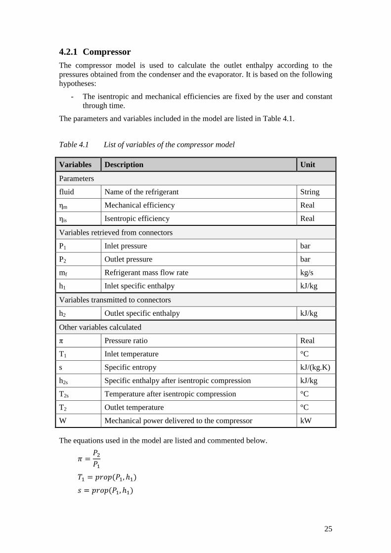
4.2.1 Compressor The compressor model is used to calculate the outlet enthalpy according to the pressures obtained from the condenser and the evaporator. It is based on the following hypotheses:

- The isentropic and mechanical efficiencies are fixed by the user and constant through time.

The parameters and variables included in the model are listed in Table 4.1.

Table 4.1 List of variables of the compressor model

Variables Description Unit

Parameters

fluid Name of the refrigerant String

ηm Mechanical efficiency Real

ηis Isentropic efficiency Real

Variables retrieved from connectors

P1 Inlet pressure bar

P2 Outlet pressure bar

mf Refrigerant mass flow rate kg/s

h1 Inlet specific enthalpy kJ/kg

Variables transmitted to connectors

h2 Outlet specific enthalpy kJ/kg

Other variables calculated

π Pressure ratio Real

T1 Inlet temperature °C

s Specific entropy kJ/(kg.K)

h2s Specific enthalpy after isentropic compression kJ/kg

T2s Temperature after isentropic compression °C

T2 Outlet temperature °C

W Mechanical power delivered to the compressor kW

The equations used in the model are listed and commented below.

= �5�6

�6 = ��-�(�6, ℎ6) � = ��-�(�6, ℎ6)

26

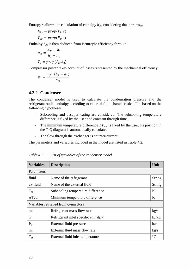
Entropy s allows the calculation of enthalpy h2s, considering that s=s1=s2s. ℎ59 = ��-�(�5, �) �59 = ��-�(�5, �) Enthalpy h2s is then deduced from isentropic efficiency formula.

�:9 = ℎ59 − ℎ6ℎ5 − ℎ6

�5 = ��-�(�5, ℎ5) Compressor power takes account of losses represented by the mechanical efficiency.

� = �� ∙ (ℎ5 − ℎ6)�=

4.2.2 Condenser The condenser model is used to calculate the condensation pressure and the refrigerant outlet enthalpy according to external fluid characteristics. It is based on the following hypotheses:

- Subcooling and desuperheating are considered. The subcooling temperature difference is fixed by the user and constant through time.

- The minimum temperature difference ∆Tmin is fixed by the user. Its position in the T-Q diagram is automatically calculated.

- The flow through the exchanger is counter-current.

The parameters and variables included in the model are listed in Table 4.2.

Table 4.2 List of variables of the condenser model

Variables Description Unit

Parameters

fluid Name of the refrigerant String

extfluid Name of the external fluid String

Tsc Subcooling temperature difference K

∆Tmin Minimum temperature difference K

Variables retrieved from connectors

mf Refrigerant mass flow rate kg/s

hfi Refrigerant inlet specific enthalpy kJ/kg

Pe External fluid pressure bar

me External fluid mass flow rate kg/s

Tei External fluid inlet temperature °C

27

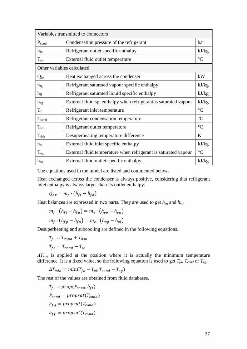
Variables transmitted to connectors

Pcond Condensation pressure of the refrigerant bar

hfo Refrigerant outlet specific enthalpy kJ/kg

Teo External fluid outlet temperature °C

Other variables calculated

Qhx Heat exchanged across the condenser kW

hfg Refrigerant saturated vapour specific enthalpy kJ/kg

hff Refrigerant saturated liquid specific enthalpy kJ/kg

heg External fluid sp. enthalpy when refrigerant is saturated vapour kJ/kg

Tfi Refrigerant inlet temperature °C

Tcond Refrigerant condensation temperature °C

Tfo Refrigerant outlet temperature °C

Tdsh Desuperheating temperature difference K

hei External fluid inlet specific enthalpy kJ/kg

Teg External fluid temperature when refrigerant is saturated vapour °C

heo External fluid outlet specific enthalpy kJ/kg

The equations used in the model are listed and commented below.

Heat exchanged across the condenser is always positive, considering that refrigerant inlet enthalpy is always larger than its outlet enthalpy. �>? = �� ∙ @ℎ�: − ℎ�AB Heat balances are expressed in two parts. They are used to get heg and heo. �� ∙ @ℎ�: − ℎ�CB = �D ∙ @ℎDA − ℎDCB �� ∙ @ℎ�C − ℎ�AB = �D ∙ @ℎDC − ℎD:B Desuperheating and subcooling are defined in the following equations. ��: = �EAFG + �G9> ��A = �EAFG − �9E ∆Tmin is applied at the position where it is actually the minimum temperature difference. It is a fixed value, so the following equation is used to get Tfo, Tcond or Teg. ∆�=:F = �*�(��A − �D:, �EAFG − �DC) The rest of the values are obtained from fluid databases. ��: = ��-�(�EAFG, ℎ�:) �EAFG = ��-��'�(�EAFG) ℎ�C = ��-��'�(�EAFG) ℎ�� = ��-��'�(�EAFG)

28

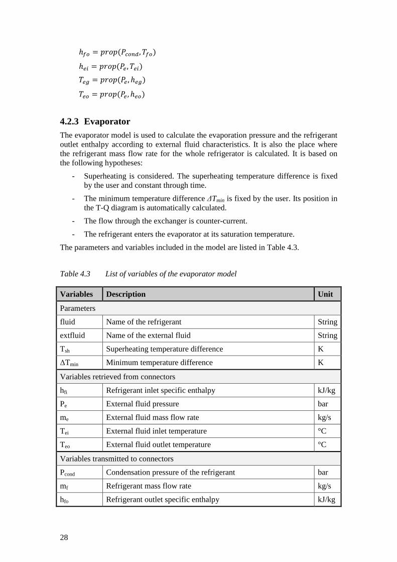
ℎ�A = ��-�(�EAFG, ��A) ℎD: = ��-�(�D , �D:) �DC = ��-�(�D , ℎDC) �DA = ��-�(�D , ℎDA)

4.2.3 Evaporator The evaporator model is used to calculate the evaporation pressure and the refrigerant outlet enthalpy according to external fluid characteristics. It is also the place where the refrigerant mass flow rate for the whole refrigerator is calculated. It is based on the following hypotheses:

- Superheating is considered. The superheating temperature difference is fixed by the user and constant through time.

- The minimum temperature difference ∆Tmin is fixed by the user. Its position in the T-Q diagram is automatically calculated.

- The flow through the exchanger is counter-current.

- The refrigerant enters the evaporator at its saturation temperature.

The parameters and variables included in the model are listed in Table 4.3.

Table 4.3 List of variables of the evaporator model

Variables Description Unit

Parameters

fluid Name of the refrigerant String

extfluid Name of the external fluid String

Tsh Superheating temperature difference K

∆Tmin Minimum temperature difference K

Variables retrieved from connectors

hfi Refrigerant inlet specific enthalpy kJ/kg

Pe External fluid pressure bar

me External fluid mass flow rate kg/s

Tei External fluid inlet temperature °C

Teo External fluid outlet temperature °C

Variables transmitted to connectors

Pcond Condensation pressure of the refrigerant bar

mf Refrigerant mass flow rate kg/s

hfo Refrigerant outlet specific enthalpy kJ/kg

29

Other variables calculated

Qhx Heat exchanged across the evaporator kW

hfg Refrigerant saturated vapour specific enthalpy kJ/kg

Tfi Refrigerant inlet temperature °C

Tevap Refrigerant evaporation temperature °C

Tfo Refrigerant outlet temperature °C

x Steam mass fraction at the inlet Real

hei External fluid inlet specific enthalpy kJ/kg

heo External fluid outlet specific enthalpy kJ/kg

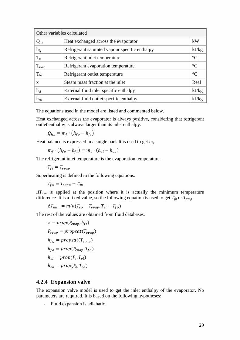
The equations used in the model are listed and commented below.

Heat exchanged across the evaporator is always positive, considering that refrigerant outlet enthalpy is always larger than its inlet enthalpy. �>? = �� ∙ @ℎ�A − ℎ�:B Heat balance is expressed in a single part. It is used to get hfo. �� ∙ @ℎ�A − ℎ�:B = �D ∙ (ℎD: − ℎDA) The refrigerant inlet temperature is the evaporation temperature. ��: = �DJKL

Superheating is defined in the following equations. ��A = �DJKL + �9>

∆Tmin is applied at the position where it is actually the minimum temperature difference. It is a fixed value, so the following equation is used to get Tfo or Tevap. ∆�=:F = �*�(�DA − �DJKL, �D: − ��A) The rest of the values are obtained from fluid databases. � = ��-�(�DJKL, ℎ�:) �DJKL = ��-��'�(�DJKL) ℎ�C = ��-��'�(�DJKL) ℎ�A = ��-�(�DJKL, ��A) ℎD: = ��-�(�D , �D:) ℎDA = ��-�(�D , �DA)

4.2.4 Expansion valve The expansion valve model is used to get the inlet enthalpy of the evaporator. No parameters are required. It is based on the following hypotheses:

- Fluid expansion is adiabatic.

30

The variables included in the model are listed in Table 4.

Table 4.4 List of variables of the expansion valve model

Variables Description

Variables retrieved from connectors

hfi Inlet specific enthalpy

Variables transmitted to connectors

hfo Outlet specific

There is only one equation used in thspecific enthalpy is equal to the inlet specific enthalpyℎ�: = ℎ�A

Note that there is no transmission of pressure and mass flow rate across the This has been done in order to avoid the loop problem evoked in Section 3.3.

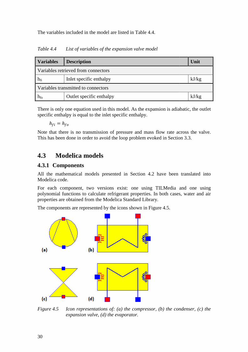
4.3 Modelica models4.3.1 Components All the mathematical models presented in Section 4.2 have been translated into Modelica code.

For each component, two versions exist: one using polynomial functions to calculate refrigerant properties. In both cases, water and air properties are obtained from the Modelica Standard Library.

The components are represented by the icons shown in Figure 4.

Figure 4.5 Icon representations of: (a) the compressor, (b) the condenser, (c) the expansion valve, (d) the evaporator.

ed in the model are listed in Table 4.4.

List of variables of the expansion valve model

Description

Variables retrieved from connectors

Inlet specific enthalpy

Variables transmitted to connectors

Outlet specific enthalpy

equation used in this model. As the expansion is adiabatic, the outlet specific enthalpy is equal to the inlet specific enthalpy.

Note that there is no transmission of pressure and mass flow rate across the This has been done in order to avoid the loop problem evoked in Section 3.3.

Modelica models

All the mathematical models presented in Section 4.2 have been translated into

For each component, two versions exist: one using TILMedia and one using polynomial functions to calculate refrigerant properties. In both cases, water and air properties are obtained from the Modelica Standard Library.

are represented by the icons shown in Figure 4.5.

representations of: (a) the compressor, (b) the condenser, (c) the expansion valve, (d) the evaporator.

Unit

kJ/kg

kJ/kg

. As the expansion is adiabatic, the outlet

Note that there is no transmission of pressure and mass flow rate across the valve. This has been done in order to avoid the loop problem evoked in Section 3.3.

All the mathematical models presented in Section 4.2 have been translated into

TILMedia and one using polynomial functions to calculate refrigerant properties. In both cases, water and air

representations of: (a) the compressor, (b) the condenser, (c) the

31

Compressor and ExpansionValve have 2 connectors:

- 1 inlet and 1 outlet for the refrigerant (P, m, h)

Condenser and Evaporator have 4 connectors:

- 1 inlet and 1 outlet for the refrigerant (P, m ,h) - 1 inlet and 1 outlet for the external fluid (P, m, T)

Connectors for refrigerant use enthalpy because phase transition is observed in the whole process. Connectors for external fluid use temperature because there is no phase transition observed and because it is more convenient for practical use. Using enthalpy everywhere would result in constant conversions between enthalpy and temperature, increasing margins of error.

Modelica codes of the models are given in Appendix 2.

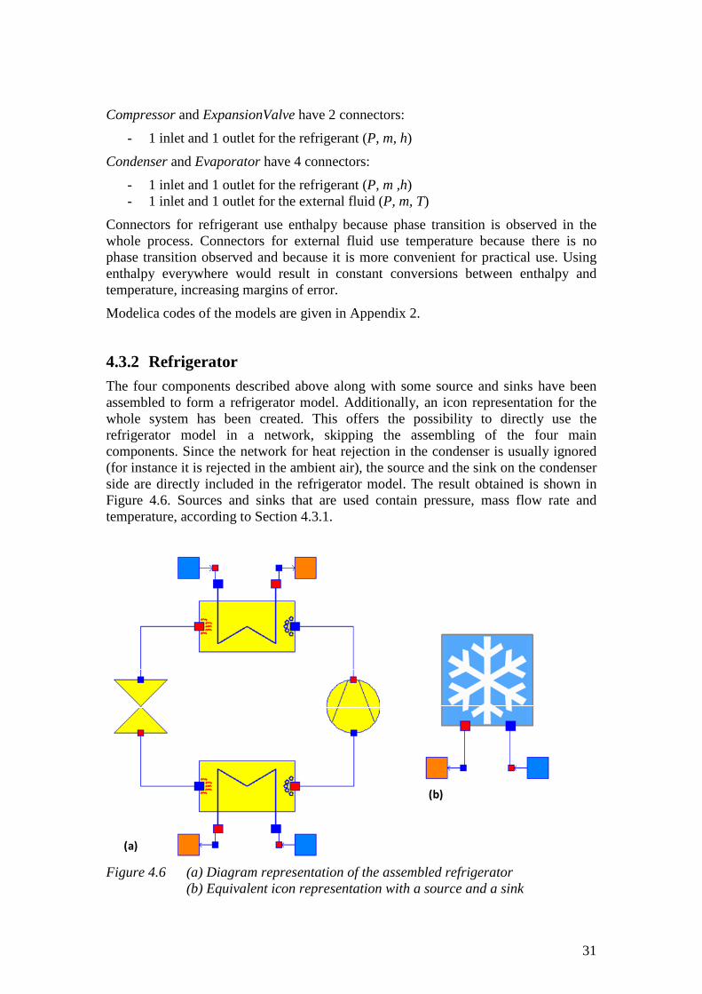
4.3.2 Refrigerator The four components described above along with some source and sinks have been assembled to form a refrigerator model. Additionally, an icon representation for the whole system has been created. This offers the possibility to directly use the refrigerator model in a network, skipping the assembling of the four main components. Since the network for heat rejection in the condenser is usually ignored (for instance it is rejected in the ambient air), the source and the sink on the condenser side are directly included in the refrigerator model. The result obtained is shown in Figure 4.6. Sources and sinks that are used contain pressure, mass flow rate and temperature, according to Section 4.3.1.

Figure 4.6 (a) Diagram representation of the assembled refrigerator (b) Equivalent icon representation with a source and a sink

(a)

(b)

32

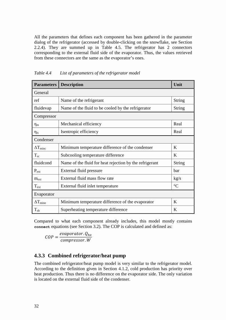
All the parameters that defines each component has been gathered in the parameter dialog of the refrigerator (accessed by double-clicking on the snowflake, see Section 2.2.4). They are summed up in Table 4.5. The refrigerator has 2 connectors corresponding to the external fluid side of the evaporator. Thus, the values retrieved from these connectors are the same as the evaporator’s ones.

Table 4.4 List of parameters of the refrigerator model

Parameters Description Unit

General

ref Name of the refrigerant String

fluidevap Name of the fluid to be cooled by the refrigerator String

Compressor

ηm Mechanical efficiency Real

ηis Isentropic efficiency Real

Condenser

∆Tminc Minimum temperature difference of the condenser K

Tsc Subcooling temperature difference K

fluidcond Name of the fluid for heat rejection by the refrigerant String

Pext External fluid pressure bar

mext External fluid mass flow rate kg/s

Text External fluid inlet temperature °C

Evaporator

∆Tmine Minimum temperature difference of the evaporator K

Tsh Superheating temperature difference K

Compared to what each component already includes, this model mostly contains connect equations (see Section 3.2). The COP is calculated and defined as:

�M� = �.'�-�'�-�. �>?+-������-�.�

4.3.3 Combined refrigerator/heat pump The combined refrigerator/heat pump model is very similar to the refrigerator model. According to the definition given in Section 4.1.2, cold production has priority over heat production. Thus there is no difference on the evaporator side. The only variation is located on the external fluid side of the condenser.

In the refrigerator, the mass flow rateare defined as parameters. The outlet temperature is deduced from calculations. In the combined refrigerator/heat pump, both inlet and outlet temperatures are defined (representing the heat demand). calculations.

An icon representation has also been Since the network for heat rejection in the condenser is of importance in this case, there is no source or sink directly inmodel. Consequently, the combined refrigerator/heat pump has 4 connectors corresponding to both external fluid sides of the evaporator and the condenser.

Figure 4.7 Icon representation of the combined

Parameters are strictly identical to the refrigerator’s ones, without Two different COPs are calculated, one on the cold side and one on the hot side.

�M�EAOG = �.'�-�'�-�+-������-��M�>AP = +-�������+-������-�

There is not a true definition of a global COP in this case. The can be added to give an idea of the overall performance of the machine.

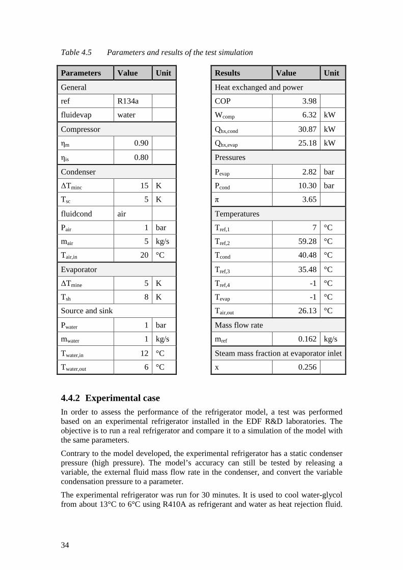
4.4 Simulations 4.4.1 Test case To illustrate the model, a simulation was done with a refrigerator connected to a source and a sink (see Figure 4.6b)12°C to 6°C using R134a as refrigerant and air as heat rejectionexchangers are set to 5K for water and 15K for air. up along with the results obtained in Table 4.5position of the refrigerant in Figure 4.1.

In the refrigerator, the mass flow rate and the inlet temperature of the external fluid are defined as parameters. The outlet temperature is deduced from calculations. In the combined refrigerator/heat pump, both inlet and outlet temperatures are defined (representing the heat demand). It is the mass flow rate that is deduced from

An icon representation has also been made for the model, as shown in Figure 4.7Since the network for heat rejection in the condenser is of importance in this case,

sink directly included in the combined refrigeratorConsequently, the combined refrigerator/heat pump has 4 connectors

corresponding to both external fluid sides of the evaporator and the condenser.

Icon representation of the combined refrigerator/heat pump

arameters are strictly identical to the refrigerator’s ones, without Pext

Two different COPs are calculated, one on the cold side and one on the hot side. �.'�-�'�-�. �>?+-������-�.�

+-�������. �>?

+-������-�.�

There is not a true definition of a global COP in this case. The COPcold can be added to give an idea of the overall performance of the machine.

and results

To illustrate the model, a simulation was done with a refrigerator connected to a (see Figure 4.6b). In this case, the purpose is to cool water from

12°C to 6°C using R134a as refrigerant and air as heat rejection fluid. exchangers are set to 5K for water and 15K for air. The input parameters are summed up along with the results obtained in Table 4.5. Subscripts 1, 2, 3 and 4 refer to the position of the refrigerant in Figure 4.1.

33

and the inlet temperature of the external fluid are defined as parameters. The outlet temperature is deduced from calculations. In the combined refrigerator/heat pump, both inlet and outlet temperatures are defined

s deduced from

, as shown in Figure 4.7. Since the network for heat rejection in the condenser is of importance in this case,

refrigerator/heat pump Consequently, the combined refrigerator/heat pump has 4 connectors

corresponding to both external fluid sides of the evaporator and the condenser.

refrigerator/heat pump

ext, mext, and Text. Two different COPs are calculated, one on the cold side and one on the hot side.

cold and the COPhot can be added to give an idea of the overall performance of the machine.

To illustrate the model, a simulation was done with a refrigerator connected to a s to cool water from

fluid. ∆Tmin in the put parameters are summed

Subscripts 1, 2, 3 and 4 refer to the

34

Table 4.5 Parameters and results of the test simulation

Parameters Value Unit __________

Results Value Unit

General Heat exchanged and power

ref R134a COP 3.98

fluidevap water Wcomp 6.32 kW

Compressor Qhx,cond 30.87 kW

ηm 0.90 Qhx,evap 25.18 kW

ηis 0.80 Pressures

Condenser Pevap 2.82 bar

∆Tminc 15 K Pcond 10.30 bar

Tsc 5 K π 3.65

fluidcond air Temperatures

Pair 1 bar Tref,1 7 °C

mair 5 kg/s Tref,2 59.28 °C

Tair,in 20 °C Tcond 40.48 °C

Evaporator Tref,3 35.48 °C

∆Tmine 5 K Tref,4 -1 °C

Tsh 8 K Tevap -1 °C

Source and sink Tair,out 26.13 °C

Pwater 1 bar Mass flow rate

mwater 1 kg/s mref 0.162 kg/s

Twater,in 12 °C Steam mass fraction at evaporator inlet

Twater,out 6 °C x 0.256

4.4.2 Experimental case In order to assess the performance of the refrigerator model, a test was performed based on an experimental refrigerator installed in the EDF R&D laboratories. The objective is to run a real refrigerator and compare it to a simulation of the model with the same parameters.

Contrary to the model developed, the experimental refrigerator has a static condenser pressure (high pressure). The model’s accuracy can still be tested by releasing a variable, the external fluid mass flow rate in the condenser, and convert the variable condensation pressure to a parameter.

The experimental refrigerator was run for 30 minutes. It is used to cool water-glycol from about 13°C to 6°C using R410A as refrigerant and water as heat rejection fluid.

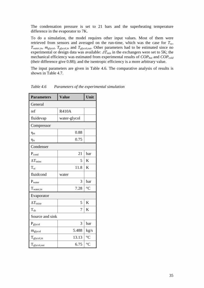
35

The condensation pressure is set to 21 bars and the superheating temperature difference in the evaporator to 7K.

To do a simulation, the model requires other input values. Most of them were retrieved from sensors and averaged on the run-time, which was the case for Tsc, Twater,in, mglycol, Tglycol,in and Tglycol,out. Other parameters had to be estimated since no experimental or design data was available: ∆Tmin in the exchangers were set to 5K; the mechanical efficiency was estimated from experimental results of COPhot and COPcold (their difference give 0.88); and the isentropic efficiency is a more arbitrary value.

The input parameters are given in Table 4.6. The comparative analysis of results is shown in Table 4.7.

Table 4.6 Parameters of the experimental simulation

Parameters Value Unit

General

ref R410A

fluidevap water-glycol

Compressor

ηm 0.88

ηis 0.75

Condenser

Pcond 21 bar

∆Tminc 5 K

Tsc 11.8 K

fluidcond water

Pwater 3 bar

Twater,in 7.28 °C

Evaporator

∆Tmine 5 K

Tsh 7 K

Source and sink

Pglycol 3 bar

mglycol 5.488 kg/s

Tglycol,in 13.13 °C

Tglycol,out 6.75 °C

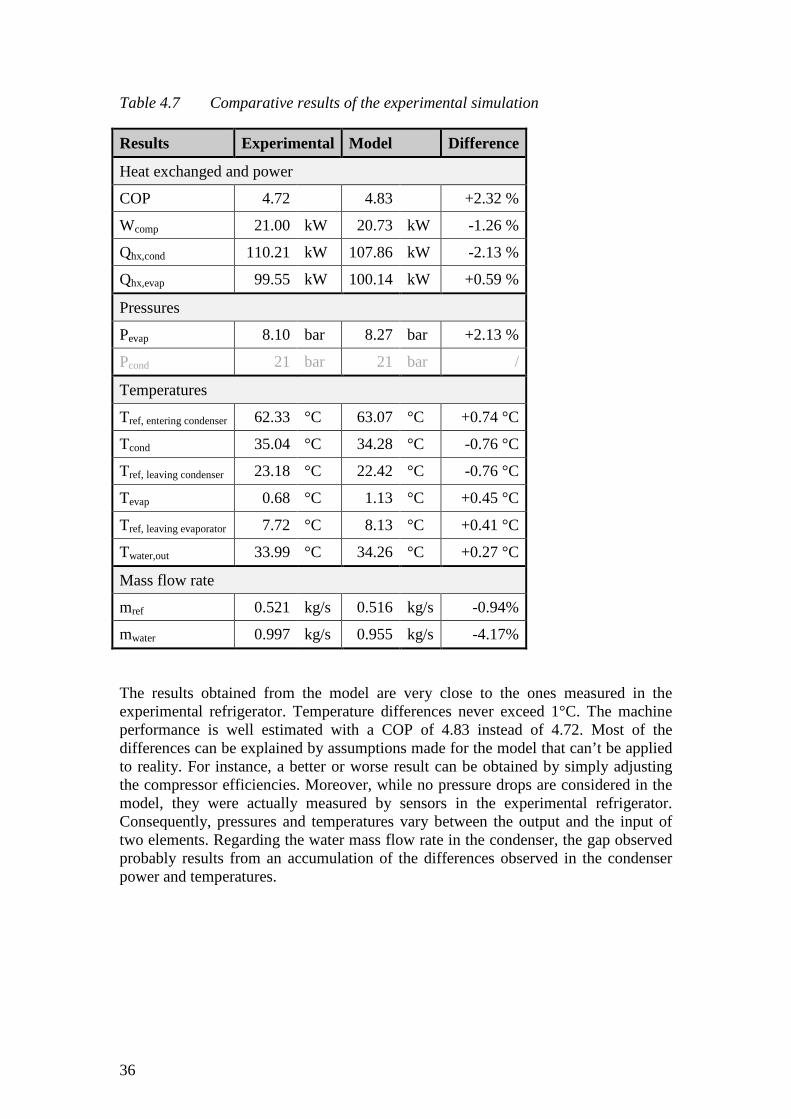
36

Table 4.7 Comparative results of the experimental simulation

Results Experimental Model Difference

Heat exchanged and power

COP 4.72 4.83 +2.32 %

Wcomp 21.00 kW 20.73 kW -1.26 %

Qhx,cond 110.21 kW 107.86 kW -2.13 %

Qhx,evap 99.55 kW 100.14 kW +0.59 %

Pressures

Pevap 8.10 bar 8.27 bar +2.13 %

Pcond 21 bar 21 bar /

Temperatures

Tref, entering condenser 62.33 °C 63.07 °C +0.74 °C

Tcond 35.04 °C 34.28 °C -0.76 °C

Tref, leaving condenser 23.18 °C 22.42 °C -0.76 °C

Tevap 0.68 °C 1.13 °C +0.45 °C

Tref, leaving evaporator 7.72 °C 8.13 °C +0.41 °C

Twater,out 33.99 °C 34.26 °C +0.27 °C

Mass flow rate

mref 0.521 kg/s 0.516 kg/s -0.94%

mwater 0.997 kg/s 0.955 kg/s -4.17%

The results obtained from the model are very close to the ones measured in the experimental refrigerator. Temperature differences never exceed 1°C. The machine performance is well estimated with a COP of 4.83 instead of 4.72. Most of the differences can be explained by assumptions made for the model that can’t be applied to reality. For instance, a better or worse result can be obtained by simply adjusting the compressor efficiencies. Moreover, while no pressure drops are considered in the model, they were actually measured by sensors in the experimental refrigerator. Consequently, pressures and temperatures vary between the output and the input of two elements. Regarding the water mass flow rate in the condenser, the gap observed probably results from an accumulation of the differences observed in the condenser power and temperatures.

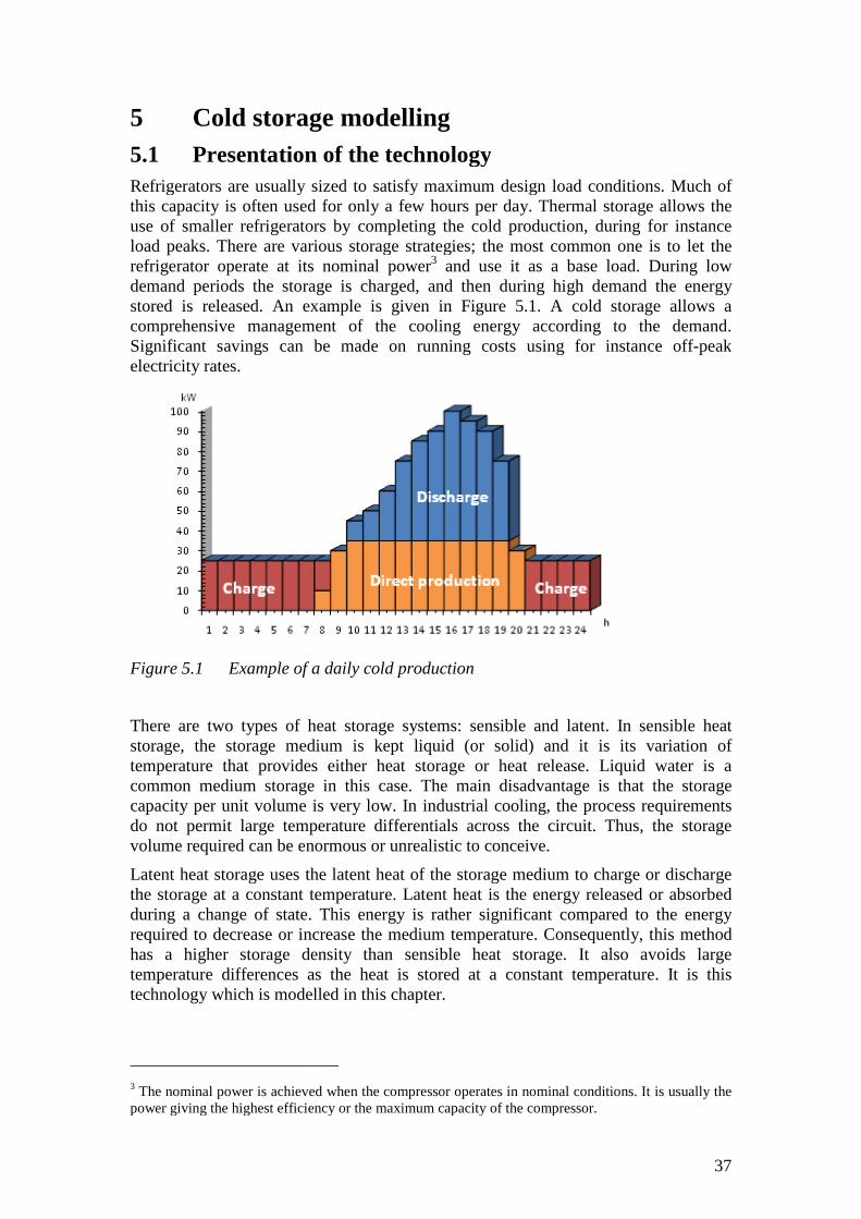
5 Cold storage modelling5.1 Presentation of the technologyRefrigerators are usually sized to satisfy maximum design load conditions. Much of this capacity is often used use of smaller refrigerators by completing the cold production, duringload peaks. There are various storage strategiesrefrigerator operate at its demand periods the storage is charged, and then during high demand the energy stored is released. An example is given in Figure 5.1. comprehensive management of the cooling energy according to the demand. Significant savings can be made on running costs using for instance offelectricity rates.

Figure 5.1 Example of a daily cold production

There are two types of heat storagestorage, the storage medium is keptemperature that provides either heat storage or heat release. common medium storage in this case. The main disadvantage is that the storage capacity per unit volume do not permit large temperature differentials across the circuit. Thusvolume required can be enormous or unrealistic to conceive.

Latent heat storage uses the latent heat of the storage medium to the storage at a constant temperature. during a change of state. required to decrease or increase the medium temperature.has a higher storage density than sensible heat storage.temperature differences as the technology which is modelled in this chapter.

3 The nominal power is achievedpower giving the highest efficiency or the maximum capacity of the compressor.

Cold storage modelling Presentation of the technology

Refrigerators are usually sized to satisfy maximum design load conditions. Much of often used for only a few hours per day. Thermal storage allows the

use of smaller refrigerators by completing the cold production, duringare various storage strategies; the most common one is to let the

refrigerator operate at its nominal power3 and use it as a base loaddemand periods the storage is charged, and then during high demand the energy

An example is given in Figure 5.1. A cold storage allows a comprehensive management of the cooling energy according to the demand.

icant savings can be made on running costs using for instance off

Example of a daily cold production

There are two types of heat storage systems: sensible and latent. In sensible heat storage, the storage medium is kept liquid (or solid) and it is itstemperature that provides either heat storage or heat release. Liquid wcommon medium storage in this case. The main disadvantage is that the storage

is very low. In industrial cooling, the process requirements do not permit large temperature differentials across the circuit. Thusvolume required can be enormous or unrealistic to conceive.

Latent heat storage uses the latent heat of the storage medium to charge or discharge at a constant temperature. Latent heat is the energy released or absorbed

during a change of state. This energy is rather significant compared to the energyrequired to decrease or increase the medium temperature. Consequentlhas a higher storage density than sensible heat storage. It also avoids large temperature differences as the heat is stored at a constant temperature.

which is modelled in this chapter.

The nominal power is achieved when the compressor operates in nominal conditions. It is usually the power giving the highest efficiency or the maximum capacity of the compressor.

37

Refrigerators are usually sized to satisfy maximum design load conditions. Much of Thermal storage allows the

use of smaller refrigerators by completing the cold production, during for instance he most common one is to let the

ase load. During low demand periods the storage is charged, and then during high demand the energy

A cold storage allows a comprehensive management of the cooling energy according to the demand.

icant savings can be made on running costs using for instance off-peak

In sensible heat its variation of

Liquid water is a common medium storage in this case. The main disadvantage is that the storage

industrial cooling, the process requirements do not permit large temperature differentials across the circuit. Thus, the storage

harge or discharge Latent heat is the energy released or absorbed

This energy is rather significant compared to the energy Consequently, this method

It also avoids large is stored at a constant temperature. It is this

when the compressor operates in nominal conditions. It is usually the

38

Two different fluids are found in a latent heat storage: a heat transfer fluid (HTF) and a phase-change material (PCM). The heat transfer fluid is the fluid that travels through the storage, being either heated (charge) or cooled (discharge). The phase-change material is the medium storage that releases cold to the HTF (discharge) or absorbs heat from it (charge).

Various latent heat storage technologies exist, differing in how the PCM is contained. The most common type of PCM containment is macro-encapsulation in which PCM is encapsulated in discrete units (Regin, Solanki, & Saini, 2008). In this thesis, the technology studied is based on a packed bed of PCM spheres. Sphere shape offers a high exchange surface with the HTF, increasing the heat transfer rate.

The storage modelled is composed of a cylindrical tank filled with nodules of same size. Nodules are spherical capsules containing PCM. Their diameter usually ranges from about 1 to 10 cm, depending on the manufacturer.

5.1.1 Mechanism The HTF flows through the voids in the bed, carrying energy from the source. During charging mode, cold HTF circulates and the PCM inside the capsules releases latent heat and crystallizes. During discharging mode, hot HTF circulates and the PCM melts. The cooled fluid is then used to meet the load either directly or through a heat exchanger.

In both operating modes (charging and discharging), the PCM is sensibly heated for a few degrees, until it reaches its phase-change temperature. After complete melting or crystallization is achieved, further heat addition from the HTF causes the PCM to superheat or subcool, thus again storing heat sensibly. The charging process continues until the PCM and the HTF attain thermal equilibrium. The difference between the mean temperature of HTF and the phase-change temperature of PCM must be sufficient to obtain a satisfactory rate of heat transfer.

A latent heat storage has different modes of operation that are described in Chapter 6.

5.1.2 Performance Several variables determine the performance of a thermal storage unit. In general, the principle governing parameters for design a PCM storage are related to the storage configuration (particle size and shape, void fraction within the bed, tank length), HTF and PCM thermal properties (latent heat, phase-change temperature, convective heat transfer coefficients), HTF flow rate, and HTF inlet temperature (Regin, Solanki, & Saini, 2008).

The most common phase-change materials used are water/ice, paraffin wax, and eutectic salts (salt hydrates). Their phase-change temperature ranges from about -30°C to 60°C.

39

5.2 Mathematical model The latent heat storage model is conceived at a system scale. It means that no internal element is modelled independently. Consequently, all the equations describing the system are gathered in only one model. The model is described thermodynamically and relies especially on temperature variations and system geometry. Other values such as heat transfer coefficients and energy stored are also calculated.

The objective is to be able to perform dynamic simulations of latent heat storage with PCM spherical capsules.

5.2.1 Hypotheses The model’s equations are based on the following assumptions:

- Pressure loss is neglected across the storage. Since pressure does not impact the calculations, it is a reasonable assumption.

- Tank geometry is considered to be cylindrical.

- Flow is laminar, axial and incompressible. It goes in one direction for the charge mode and the other for the discharge mode.

- Variation of temperature of the heat transfer fluid is only along the axial direction; temperature is independent of radial position.

- HTF and PCM properties (Cp, ρ, k and ν) are set constant and do not vary with temperature.

- Nodules are considered as exchangers. The heat exchanged is proportional to the difference of temperature between the fluid and the PCM.

- PCM capsules behave as a continuous porous medium and not as a medium composed of individual particles.

- Temperature inside the PCM capsules is homogeneous.

- PCM melts or crystallize at a constant phase-change temperature. Phase-change does not take place in a melting temperature range. This is a realistic assumption for eutectic mixtures (Mehling & Cabeza, 2008).

- The mass and volume of the nodules’ envelope are neglected. The PCM inside the nodules is considered as PCM spheres. Consequently, PCM density represents the mass of PCM spheres per unit of volume. If data is available for solid and liquid densities, the liquid one should be used to be closer to the real PCM mass in a nodule.

- Effects of conduction across the envelope and natural convection inside the PCM nodules are neglected. PCM thermal conductivity is not considered during calculations (see Section 7.1.4 for further explanations).

- PCM and HTF have the same initial temperature everywhere in the storage.

5.2.2 Parameters The parameters that need to be specified are listed in Table 5.1. Units are not always SI and have been chosen in order to facilitate the reading of results.

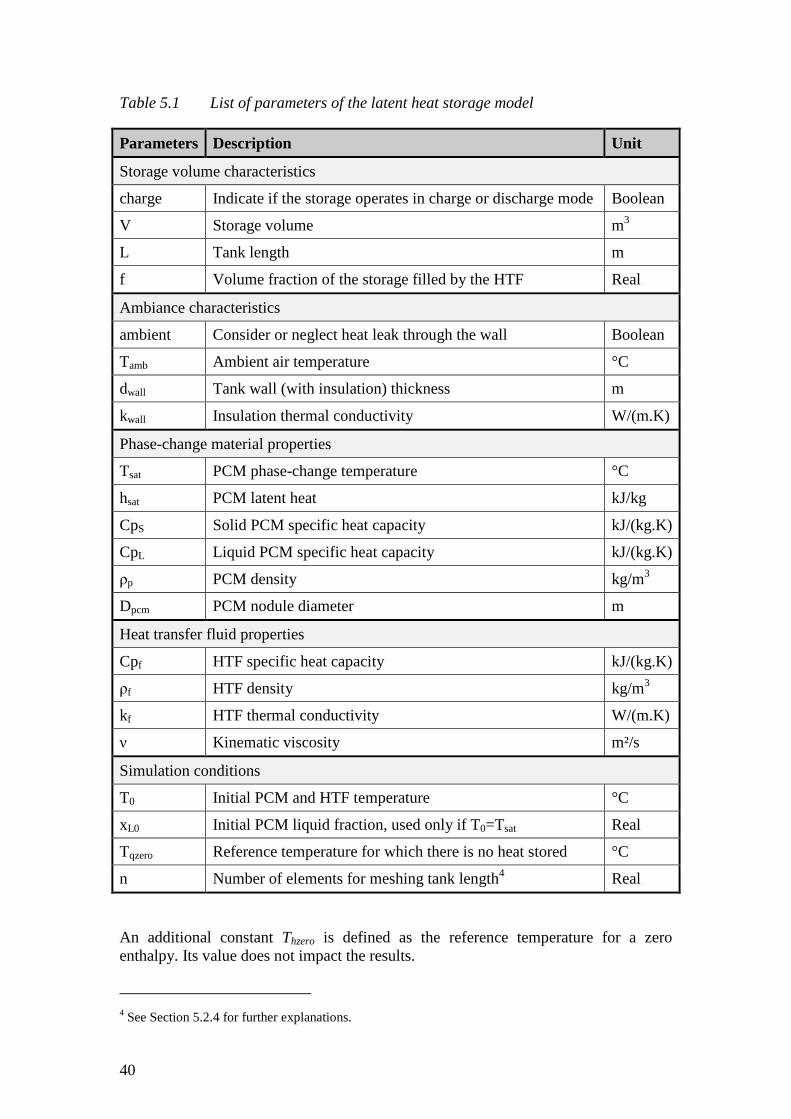
40

Table 5.1 List of parameters of the latent heat storage model

Parameters Description Unit

Storage volume characteristics

charge Indicate if the storage operates in charge or discharge mode Boolean

V Storage volume m3

L Tank length m

f Volume fraction of the storage filled by the HTF Real

Ambiance characteristics

ambient Consider or neglect heat leak through the wall Boolean

Tamb Ambient air temperature °C

dwall Tank wall (with insulation) thickness m

kwall Insulation thermal conductivity W/(m.K)

Phase-change material properties

Tsat PCM phase-change temperature °C

hsat PCM latent heat kJ/kg

CpS Solid PCM specific heat capacity kJ/(kg.K)

CpL Liquid PCM specific heat capacity kJ/(kg.K)

ρp PCM density kg/m3

Dpcm PCM nodule diameter m

Heat transfer fluid properties

Cpf HTF specific heat capacity kJ/(kg.K)

ρf HTF density kg/m3

kf HTF thermal conductivity W/(m.K)

ν Kinematic viscosity m²/s

Simulation conditions

T0 Initial PCM and HTF temperature °C

xL0 Initial PCM liquid fraction, used only if T0=Tsat Real

Tqzero Reference temperature for which there is no heat stored °C

n Number of elements for meshing tank length4 Real

An additional constant Thzero is defined as the reference temperature for a zero enthalpy. Its value does not impact the results.

4 See Section 5.2.4 for further explanations.

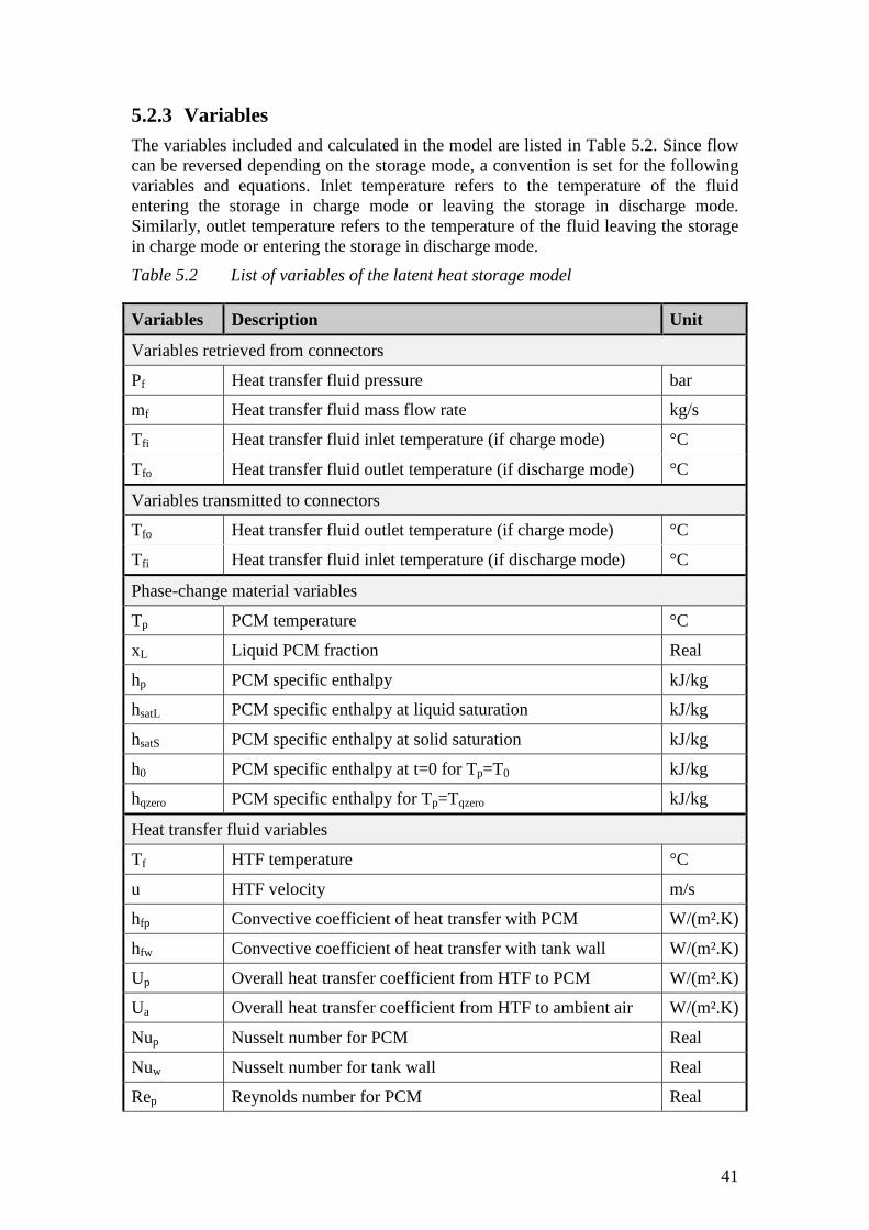
41

5.2.3 Variables The variables included and calculated in the model are listed in Table 5.2. Since flow can be reversed depending on the storage mode, a convention is set for the following variables and equations. Inlet temperature refers to the temperature of the fluid entering the storage in charge mode or leaving the storage in discharge mode. Similarly, outlet temperature refers to the temperature of the fluid leaving the storage in charge mode or entering the storage in discharge mode.

Table 5.2 List of variables of the latent heat storage model

Variables Description Unit

Variables retrieved from connectors

Pf Heat transfer fluid pressure bar

mf Heat transfer fluid mass flow rate kg/s

Tfi Heat transfer fluid inlet temperature (if charge mode) °C

Tfo Heat transfer fluid outlet temperature (if discharge mode) °C

Variables transmitted to connectors

Tfo Heat transfer fluid outlet temperature (if charge mode) °C

Tfi Heat transfer fluid inlet temperature (if discharge mode) °C

Phase-change material variables

Tp PCM temperature °C

xL Liquid PCM fraction Real

hp PCM specific enthalpy kJ/kg

hsatL PCM specific enthalpy at liquid saturation kJ/kg

hsatS PCM specific enthalpy at solid saturation kJ/kg

h0 PCM specific enthalpy at t=0 for Tp=T0 kJ/kg

hqzero PCM specific enthalpy for Tp=Tqzero kJ/kg

Heat transfer fluid variables

Tf HTF temperature °C

u HTF velocity m/s

hfp Convective coefficient of heat transfer with PCM W/(m².K)

hfw Convective coefficient of heat transfer with tank wall W/(m².K)

Up Overall heat transfer coefficient from HTF to PCM W/(m².K)

Ua Overall heat transfer coefficient from HTF to ambient air W/(m².K)

Nup Nusselt number for PCM Real

Nuw Nusselt number for tank wall Real

Rep Reynolds number for PCM Real

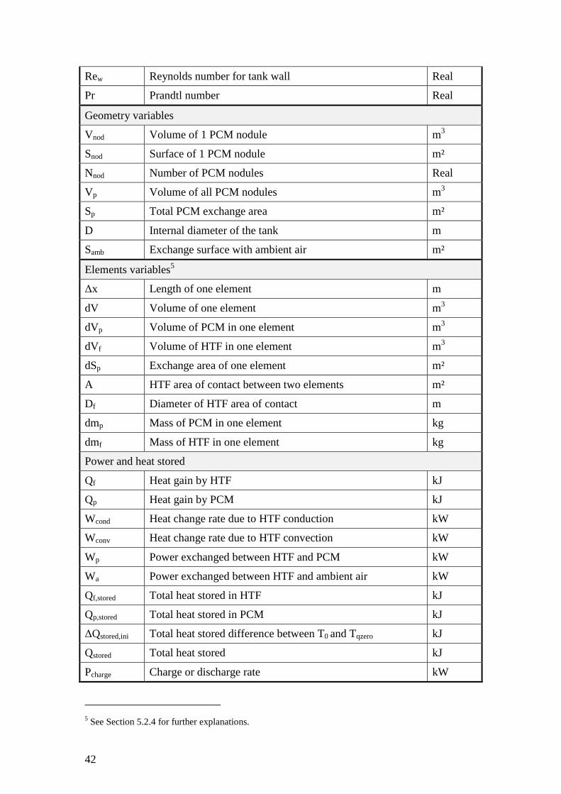
42

Rew Reynolds number for tank wall Real

Pr Prandtl number Real

Geometry variables

Vnod Volume of 1 PCM nodule m3

Snod Surface of 1 PCM nodule m²

Nnod Number of PCM nodules Real

Vp Volume of all PCM nodules m3

Sp Total PCM exchange area m²

D Internal diameter of the tank m

Samb Exchange surface with ambient air m²

Elements variables5

∆x Length of one element m

dV Volume of one element m3

dVp Volume of PCM in one element m3

dVf Volume of HTF in one element m3

dSp Exchange area of one element m²

A HTF area of contact between two elements m²

Df Diameter of HTF area of contact m

dmp Mass of PCM in one element kg

dmf Mass of HTF in one element kg

Power and heat stored

Qf Heat gain by HTF kJ

Qp Heat gain by PCM kJ

Wcond Heat change rate due to HTF conduction kW

Wconv Heat change rate due to HTF convection kW

Wp Power exchanged between HTF and PCM kW

Wa Power exchanged between HTF and ambient air kW

Qf,stored Total heat stored in HTF kJ

Qp,stored Total heat stored in PCM kJ

∆Qstored,ini Total heat stored difference between T0 and Tqzero kJ

Qstored Total heat stored kJ

Pcharge Charge or discharge rate kW

5 See Section 5.2.4 for further explanations.

43

5.2.4 Mesh The model is based on the mathematical model developed by Wu et al. and describing a heat storage system with PCM in spherical capsules (Wu, Fang, & Liu, 2011). The conservation equation for the heat transfer fluid is written as:

∙ !� ∙ ��� ∙ Q��Q�RSSSSTSSSSU>DKPE>KFCDWKPDA�XYZ= ∙ �� ∙ Q5��Q�5RSSTSSUD��DEPA�EAFG[EP:AF

− ∙ !� ∙ ��� ∙ � ∙ Q��Q�RSSSSSTSSSSSUD��DEPA�EAFJDEP:AF+ �L ∙ �L� ∙ @�L − ��BRSSSSTSSSSUDFDWC\PWKF9�DW]:P>^_`

− �K ∙ �K=a� ∙ (�� − �K=a)RSSSSSSTSSSSSSUDFDWC\PWKF9�DW]:P>K=a:DFPK:W

where x is the location of the flow direction and t is time. Each term is described in the equation.

The conservation equation for the phase-change material depends on its state:

�L ∙ �L� ∙ @�� − �LB =bccdcce(1 − ) ∙ !L ∙ ��f ∙ Q�LQ� ifPCMinsolidphase(1 − ) ∙ !L ∙ ℎ9KP ∙ Q��Q� ifPCMinphasetransition(1 − ) ∙ !L ∙ ��� ∙ Q�LQ� ifPCMinliquidphase

y

These equations use partial derivatives. Presently, there is no simulation support available in Modelica for solving partial differential equations (PDEs) problems. Only ordinary differential equations (ODEs) can be solved (Modelica Association, 2010). It is however possible to handle PDE models by using a finite difference method. This method transforms a PDE into a system of ODEs involving only time-dependent variables and time-derivatives. This is achieved by discretizing variables that depend on other variables than time (Li, Zheng, & Zhang, 2008).

In the latent heat storage model, Tf depends on a spatial variable, x. The domain of simulation (the tank cylinder) is meshed in n elements along the axial flow direction as shown in Figure 5.2.

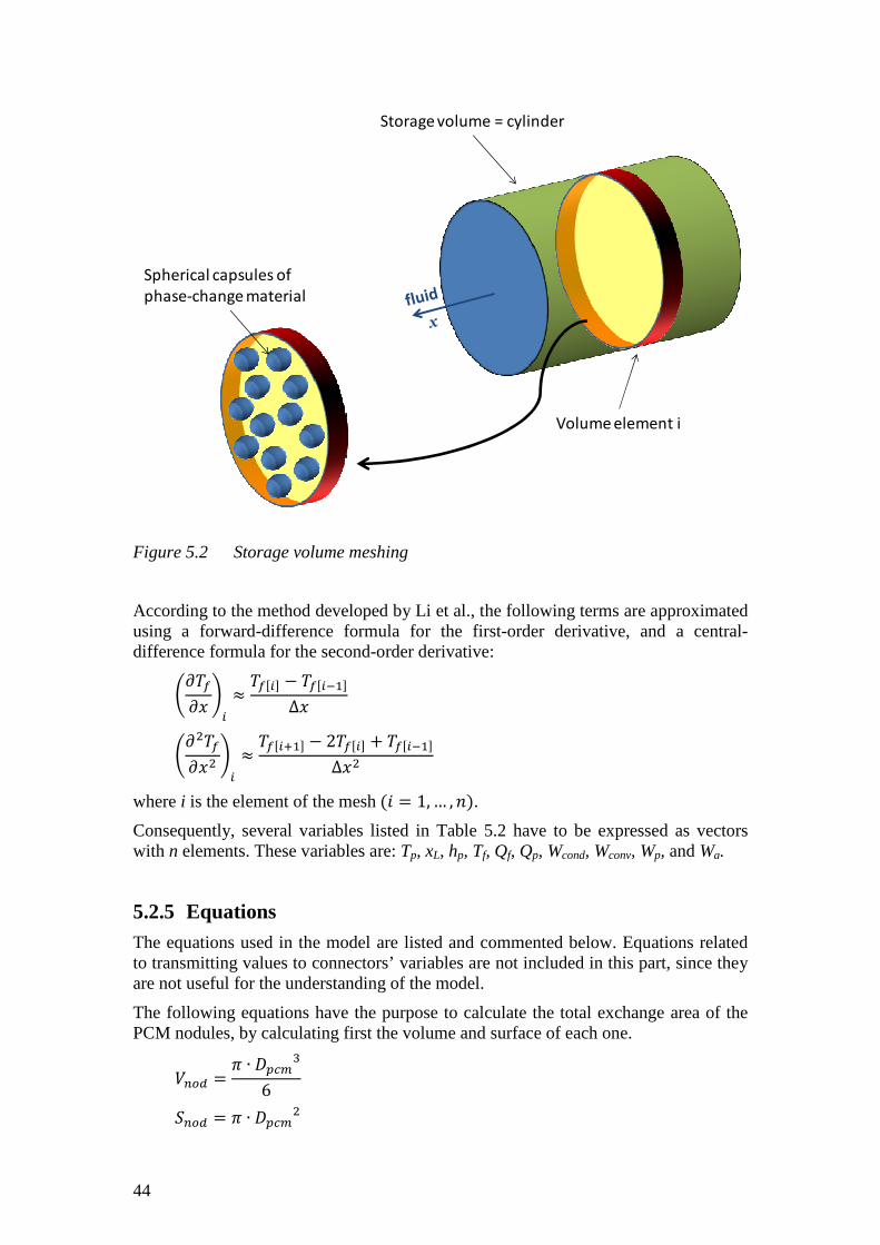
44

Figure 5.2 Storage volume meshing

According to the method developed by Li et al., the following terms are approximated using a forward-difference formula for the first-order derivative, and a central-difference formula for the second-order derivative:

zQ��Q� {: ≈��}:~ − ��}:�6~Δ�

zQ5��Q�5 {: ≈��}:�6~ − 2��}:~ + ��}:�6~Δ�5

where i is the element of the mesh(* = 1,… , �). Consequently, several variables listed in Table 5.2 have to be expressed as vectors with n elements. These variables are: Tp, xL, hp, Tf, Qf, Qp, Wcond, Wconv, Wp, and Wa.

5.2.5 Equations The equations used in the model are listed and commented below. Equations related to transmitting values to connectors’ variables are not included in this part, since they are not useful for the understanding of the model.

The following equations have the purpose to calculate the total exchange area of the PCM nodules, by calculating first the volume and surface of each one.

�FAG = ∙ �LE=�6

�FAG = ∙ �LE=5

Storage volume = cylinder

Volume element i

Spherical capsules of

phase-change material

45

�FAG = �L�FAG

�L = (1 − ) ∙ �

�L = �L ∙ �FAG�FAG

Another surface required is the exchange area with ambient air, which is actually the surface of the cylindrical tank. It is based on the internal diameter D calculated from tank volume and tank length.

� = ∙ �54 ∙

�K=a = ∙ � ∙ + 2 ∙ ∙ �54

The tank is meshed in n elements. Element volumes, surfaces and masses are calculated below.

Δ� = �

�� = ��

��L = �L�

��� = ∙ ��

��L = ��L ∙ �FAG�FAG

��L = ��L ∙ !L ��� = ��� ∙ !�

A is the area of contact between two elements i and i+1 . It is a virtual area that is based on the volume taken by the fluid only. It is therefore different from the area based on the internal diameter D. As a result, a virtual diameter Df corresponding to the area A is defined.

� = ���Δ� z= ∙ � = ∙ ∙ �54 {

�� = �4�

To calculate heat transfer coefficients, dimensionless numbers such as Prandtl, Nusselt and Reynolds are estimated. Heat transfer fluid velocity u is required and based on the area A previously obtained.

� = ��!� ∙ �

46

Reynolds and Nusselt numbers are calculated for convection of HTF on PCM and for convection of HTF on tank wall. Prandtl number remains the same for both cases. Dpcm is the characteristic length for PCM. Df is the characteristic length for tank wall.

�� = ��� ∙ ���

��L = !� ∙ � ∙ �LE=�

��] = !� ∙ � ∙ ���

��L = 2.0 + 2.03 ∙ ��L6/5 ∙ ��6/� + 0.049 ∙ ��L ∙ ��6/5 ��] = 3.657 + 0.19 ∙ ��� ∙ ��] ∙ ����.�

1 + 0.117 ∙ ��� ∙ ��] ∙ ����.��� Nup is based on a correlation developed by Galloway and Sage (Galloway & Sage, 1970) and improved by Beasley and Clark (Beasley & Clark, 1984). Nuw is based on a correlation developed by Hausen (average Nusselt number for laminar flow in a circular tube with uniform surface temperature) (Hausen, 1959).

Convective and overall heat transfer coefficients can then be calculated. Since thermal conductivity of PCM is not considered, Up has a simpler expression than Ua.

ℎ�L = �� ∙ ��L�LE=

ℎ�] = �� ∙ ��]��

�L = ℎ�L

�K = ℎ�]1 + ℎ�] ∙ �]KOO�]KOO

Each term of the conservation equation for the HTF presented in Section 5.2.4 is represented by a single variable to facilitate the reading of results and the analysis of their respective influence. Q��Q� = �EAFG +�EAFJ +�L −�K

Q��}:~Q� = ��� ∙ ��� ∙ Q��}:~Q� for* ∈ 1: �

�EAFG}:~ = � ∙ �� ∙ ��}:�6~ − 2��}:~ + ��}:�6~Δ�5 for* ∈ 1: �

�EAFJ}:~ =bcdce−��� ∙ ��� ∙ � ∙ ��}:~ − ��}:�6~Δ� for* ∈ 1: �,ifcharge−��� ∙ ��� ∙ � ∙

��[:] − ��[:�6]

Δ�for* ∈ 1: �,ifdischarge

y

47

The difference between charge and discharge for the convection term is due to the fact that the flow goes in the opposite direction, from element i+1 to element i. �L}:~ = �L ∙ �L ∙ @�L}:~ − ��}:~Bfor* ∈ 1: � Q�L}:~Q� = −�L}:~for* ∈ 1: �

To calculate Wp, two constant enthalpies are used to check in which state the PCM is: ℎ9KP� = ��f ∙ (�9KP − �>�DWA) + ℎ9KP ℎ9KPf = ��f ∙ (�9KP − �>�DWA) Using an if-condition, Wp, hp and xL (or Tp) are obtained. Since Modelica is acausal, it is possible to have an if-condition on a variable that is calculated inside. All the equations below are applied for* ∈ 1: �.

ifℎL}:~ < ℎ9KPfbccdcce�L}:~ = −��L ∙ ��f ∙ Q�L}:~Q�ℎL}:~ = ��f ∙ @�L}:~ − �>�DWAB��}:~ = 0

y

elseifℎL}:~ > ℎ9KP�bccdcce�L}:~ = −��L ∙ ��� ∙ Q�L}:~Q�ℎL}:~ = ��f ∙ (�9KP − �>�DWA) + ℎ9KP + ��� ∙ (�L}:~ − �9KP)��}:~ = 1

y

elsebccdcce�L}:~ = −��L ∙ ℎ9KP ∙ Q��}:~Q�ℎL}:~ = ��f ∙ (�9KP − �>�DWA) + ℎ9KP ∙ ��}:~�L}:~ = �9KP

y

It is possible to consider or neglect the heat leak through the wall. This option is useful if data about insulating are not available.

�K}:~ = �K ∙ �K=a� ∙ (��}:~ − �K=a)for* ∈ 1: �

Several equations contain derivatives. The differentiated variables should then be initialized at t=0. ��(� = 0) = �� �L(� = 0) = ��

���(� = 0) = ���if�� = �9KP�L(� = 0) = ��else y ��(� = 0) = 0

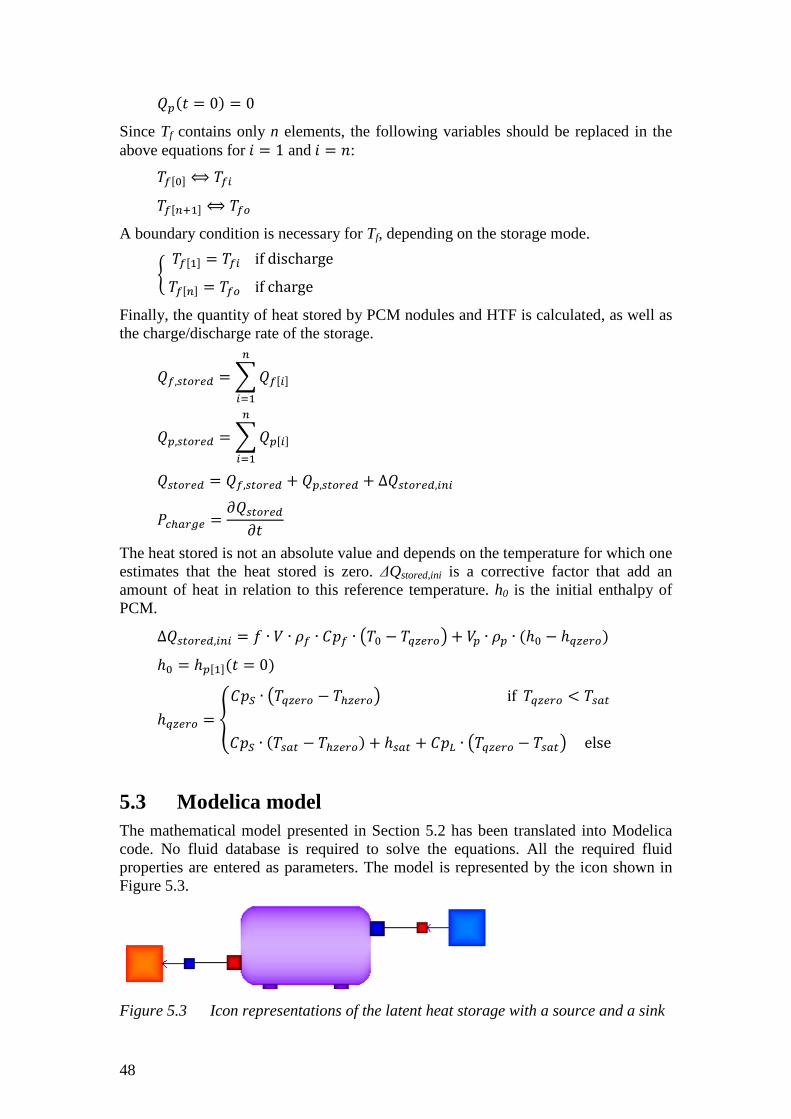
48

�L(� = 08 4 0

Since Tf contains only n elements, the following variables should be replaced in the above equations for* 4 1 ��}�~ ⟺ ��: ��}F�6~ ⟺ ��A A boundary condition is necessary for

� ��}6~ 4 ��:ifdischarge��}F~ 4 ��AifchargFinally, the quantity of heat storedthe charge/discharge rate of the storage

��,9PAWDG 4���}:~F:�6

�L,9PAWDG 4��L}:~F:�6�9PAWDG 4 ��,9PAWDG

�E>KWCD 4 Q�9PAWDGQ�

The heat stored is not an absolute valueestimates that the heat stored is zero. amount of heat in relation PCM. Δ�9PAWDG,:F: 4 ∙ �� 4 L}6~7� 4 08

��DWA 4 ���f ∙ @���DWA��f ∙ 7�9KP

5.3 Modelica modelThe mathematical model presented in Section 5.2 has been translated into Modelica code. No fluid database is requiredproperties are entered as parameters. The model is represented by the icon shown in Figure 5.3.

Figure 5.3 Icon representations of the latent heat storage

elements, the following variables should be replaced in the and* 4 �:

is necessary for Tf, depending on the storage mode.ifdischargeifcharge y Finally, the quantity of heat stored by PCM nodules and HTF is calculated

rate of the storage.

} ~

} ~ H �L,9PAWDG H Δ�9PAWDG,:F:

is not an absolute value and depends on the temperature estimates that the heat stored is zero. ∆Qstored,ini is a corrective factor that add an amount of heat in relation to this reference temperature. h0 is the initial enthalpy of

∙ !� ∙ ��� ∙ @�� ; ���DWAB H �L ∙ !L ∙ 7� ; ��DWA@ ��DWA ; �>�DWABif���DWA �7 9KP ; �>�DWA8 H 9KP H ��� ∙ @���DWA ; �9KPB

Modelica model The mathematical model presented in Section 5.2 has been translated into Modelica code. No fluid database is required to solve the equations. All the reqproperties are entered as parameters. The model is represented by the icon shown in

Icon representations of the latent heat storage with a source and a sink

elements, the following variables should be replaced in the

, depending on the storage mode.

by PCM nodules and HTF is calculated, as well as

and depends on the temperature for which one is a corrective factor that add an

is the initial enthalpy of

��DWA8 � �9KPBelsey

The mathematical model presented in Section 5.2 has been translated into Modelica to solve the equations. All the required fluid

properties are entered as parameters. The model is represented by the icon shown in

with a source and a sink

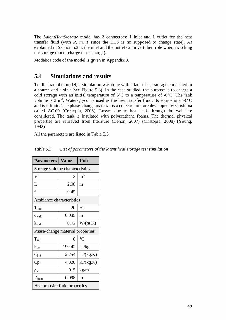
49

The LatentHeatStorage model has 2 connectors: 1 inlet and 1 outlet for the heat transfer fluid (with P, m, T since the HTF is no supposed to change state). As explained in Section 5.2.3, the inlet and the outlet can invert their role when switching the storage mode (charge or discharge).

Modelica code of the model is given in Appendix 3.

5.4 Simulations and results To illustrate the model, a simulation was done with a latent heat storage connected to a source and a sink (see Figure 5.3). In the case studied, the purpose is to charge a cold storage with an initial temperature of 6°C to a temperature of -6°C. The tank volume is 2 m3. Water-glycol is used as the heat transfer fluid. Its source is at -6°C and is infinite. The phase-change material is a eutectic mixture developed by Cristopia called AC.00 (Cristopia, 2008). Losses due to heat leak through the wall are considered. The tank is insulated with polyurethane foams. The thermal physical properties are retrieved from literature (Dehon, 2007) (Cristopia, 2008) (Young, 1992).

All the parameters are listed in Table 5.3.

Table 5.3 List of parameters of the latent heat storage test simulation

Parameters Value Unit

Storage volume characteristics

V 2 m3

L 2.98 m

f 0.45

Ambiance characteristics

Tamb 20 °C

dwall 0.035 m

kwall 0.02 W/(m.K)

Phase-change material properties

Tsat 0 °C

hsat 190.42 kJ/kg

CpS 2.754 kJ/(kg.K)

CpL 4.328 kJ/(kg.K)

ρp 915 kg/m3

Dpcm 0.098 m

Heat transfer fluid properties

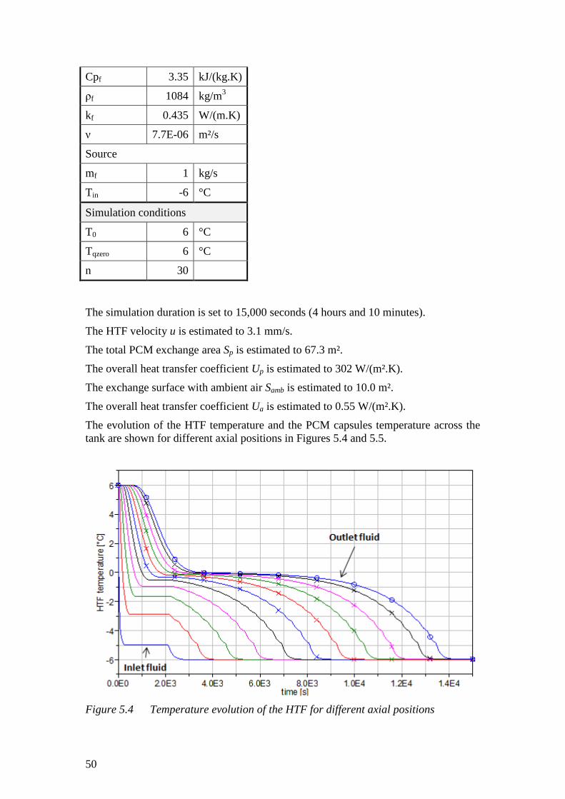
50

Cpf 3.35 kJ/(kg.K)

ρf 1084 kg/m3

kf 0.435 W/(m.K)

ν 7.7E-06 m²/s

Source

mf 1 kg/s

Tin -6 °C

Simulation conditions

T0 6 °C

Tqzero 6 °C

n 30

The simulation duration is set to 15,000 seconds (4 hours and 10 minutes).

The HTF velocity u is estimated to 3.1 mm/s.

The total PCM exchange area Sp is estimated to 67.3 m².

The overall heat transfer coefficient Up is estimated to 302 W/(m².K).

The exchange surface with ambient air Samb is estimated to 10.0 m².

The overall heat transfer coefficient Ua is estimated to 0.55 W/(m².K).

The evolution of the HTF temperature and the PCM capsules temperature across the tank are shown for different axial positions in Figures 5.4 and 5.5.

Figure 5.4 Temperature evolution of the HTF for different axial positions

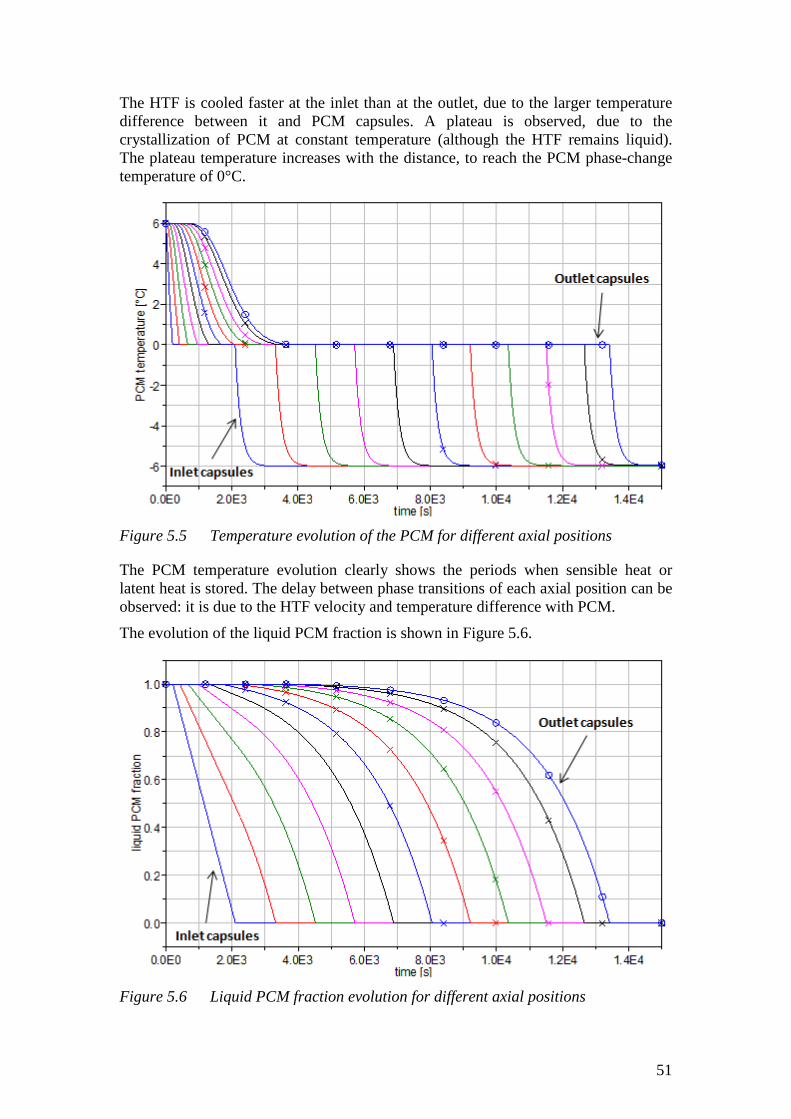
51

The HTF is cooled faster at the inlet than at the outlet, due to the larger temperature difference between it and PCM capsules. A plateau is observed, due to the crystallization of PCM at constant temperature (although the HTF remains liquid). The plateau temperature increases with the distance, to reach the PCM phase-change temperature of 0°C.

Figure 5.5 Temperature evolution of the PCM for different axial positions

The PCM temperature evolution clearly shows the periods when sensible heat or latent heat is stored. The delay between phase transitions of each axial position can be observed: it is due to the HTF velocity and temperature difference with PCM.

The evolution of the liquid PCM fraction is shown in Figure 5.6.

Figure 5.6 Liquid PCM fraction evolution for different axial positions

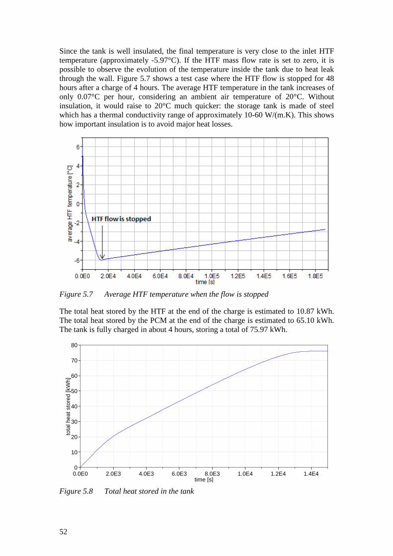
52

Since the tank is well insulated, the final temperature is very close to the inlet HTF temperature (approximately -5.97°C). If the HTF mass flow rate is set to zero, it is possible to observe the evolution of the temperature inside the tank due to heat leak through the wall. Figure 5.7 shows a test case where the HTF flow is stopped for 48 hours after a charge of 4 hours. The average HTF temperature in the tank increases of only 0.07°C per hour, considering an ambient air temperature of 20°C. Without insulation, it would raise to 20°C much quicker: the storage tank is made of steel which has a thermal conductivity range of approximately 10-60 W/(m.K). This shows how important insulation is to avoid major heat losses.

Figure 5.7 Average HTF temperature when the flow is stopped

The total heat stored by the HTF at the end of the charge is estimated to 10.87 kWh. The total heat stored by the PCM at the end of the charge is estimated to 65.10 kWh. The tank is fully charged in about 4 hours, storing a total of 75.97 kWh.

Figure 5.8 Total heat stored in the tank

0.0E0 2.0E3 4.0E3 6.0E3 8.0E3 1.0E4 1.2E4 1.4E40

10

20

30

40

50

60

70

80

tota

l hea

t sto

red

[kW

h]

time [s]

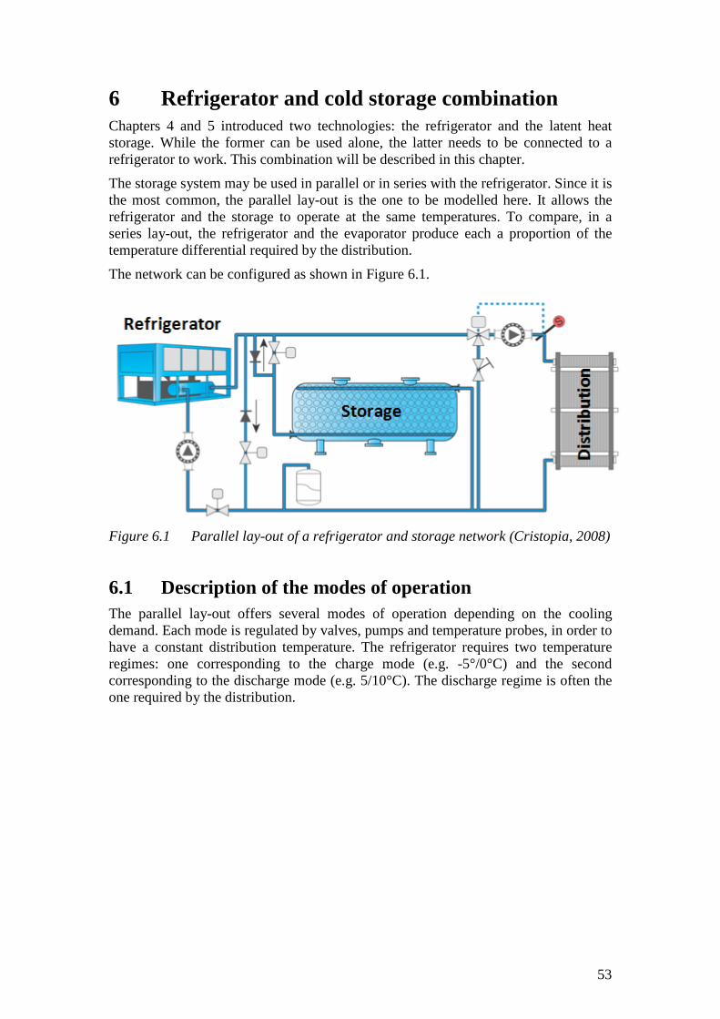
53

6 Refrigerator and cold storage combination Chapters 4 and 5 introduced two technologies: the refrigerator and the latent heat storage. While the former can be used alone, the latter needs to be connected to a refrigerator to work. This combination will be described in this chapter.

The storage system may be used in parallel or in series with the refrigerator. Since it is the most common, the parallel lay-out is the one to be modelled here. It allows the refrigerator and the storage to operate at the same temperatures. To compare, in a series lay-out, the refrigerator and the evaporator produce each a proportion of the temperature differential required by the distribution.

The network can be configured as shown in Figure 6.1.

Figure 6.1 Parallel lay-out of a refrigerator and storage network (Cristopia, 2008)

6.1 Description of the modes of operation The parallel lay-out offers several modes of operation depending on the cooling demand. Each mode is regulated by valves, pumps and temperature probes, in order to have a constant distribution temperature. The refrigerator requires two temperature regimes: one corresponding to the charge mode (e.g. -5°/0°C) and the second corresponding to the discharge mode (e.g. 5/10°C). The discharge regime is often the one required by the distribution.

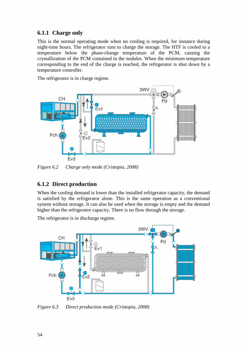
54

6.1.1 Charge only This is the normal operating mode when no cooling is required, for instance during night-time hours. The refrigerator runs to charge the storage. The HTF is cooled to a temperature below the phase-change temperature of the PCM, causing the crystallization of the PCM contained in the nodules. When the minimum temperature corresponding to the end of the charge is reached, the refrigerator is shut down by a temperature controller.

The refrigerator is in charge regime.

Figure 6.2 Charge only mode (Cristopia, 2008)

6.1.2 Direct production When the cooling demand is lower than the installed refrigerator capacity, the demand is satisfied by the refrigerator alone. This is the same operation as a conventional system without storage. It can also be used when the storage is empty and the demand higher than the refrigerator capacity. There is no flow through the storage.

The refrigerator is in discharge regime.

Figure 6.3 Direct production mode (Cristopia, 2008)

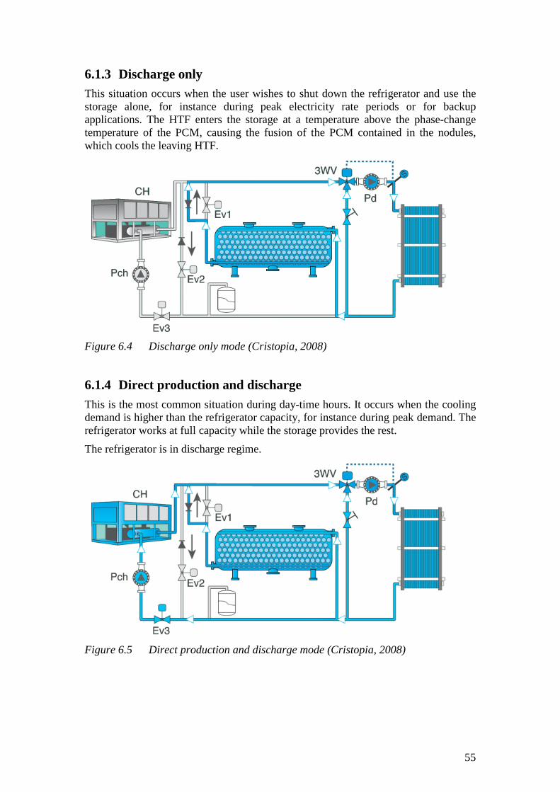
55

6.1.3 Discharge only This situation occurs when the user wishes to shut down the refrigerator and use the storage alone, for instance during peak electricity rate periods or for backup applications. The HTF enters the storage at a temperature above the phase-change temperature of the PCM, causing the fusion of the PCM contained in the nodules, which cools the leaving HTF.

Figure 6.4 Discharge only mode (Cristopia, 2008)

6.1.4 Direct production and discharge This is the most common situation during day-time hours. It occurs when the cooling demand is higher than the refrigerator capacity, for instance during peak demand. The refrigerator works at full capacity while the storage provides the rest.

The refrigerator is in discharge regime.

Figure 6.5 Direct production and discharge mode (Cristopia, 2008)

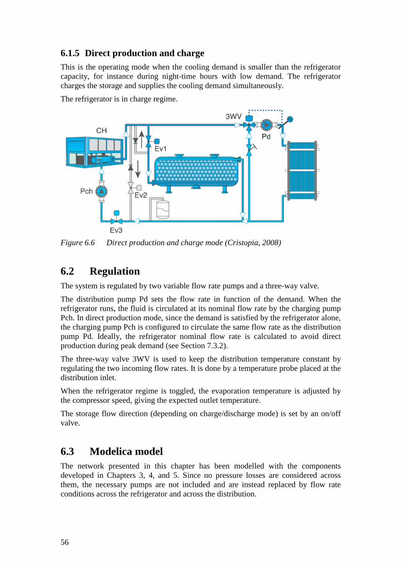
56

6.1.5 Direct production and charge This is the operating mode when the cooling demand is smaller than the refrigerator capacity, for instance during night-time hours with low demand. The refrigerator charges the storage and supplies the cooling demand simultaneously.

The refrigerator is in charge regime.

Figure 6.6 Direct production and charge mode (Cristopia, 2008)

6.2 Regulation The system is regulated by two variable flow rate pumps and a three-way valve.

The distribution pump Pd sets the flow rate in function of the demand. When the refrigerator runs, the fluid is circulated at its nominal flow rate by the charging pump Pch. In direct production mode, since the demand is satisfied by the refrigerator alone, the charging pump Pch is configured to circulate the same flow rate as the distribution pump Pd. Ideally, the refrigerator nominal flow rate is calculated to avoid direct production during peak demand (see Section 7.3.2).

The three-way valve 3WV is used to keep the distribution temperature constant by regulating the two incoming flow rates. It is done by a temperature probe placed at the distribution inlet.

When the refrigerator regime is toggled, the evaporation temperature is adjusted by the compressor speed, giving the expected outlet temperature.

The storage flow direction (depending on charge/discharge mode) is set by an on/off valve.

6.3 Modelica model The network presented in this chapter has been modelled with the components developed in Chapters 3, 4, and 5. Since no pressure losses are considered across them, the necessary pumps are not included and are instead replaced by flow rate conditions across the refrigerator and across the distribution.

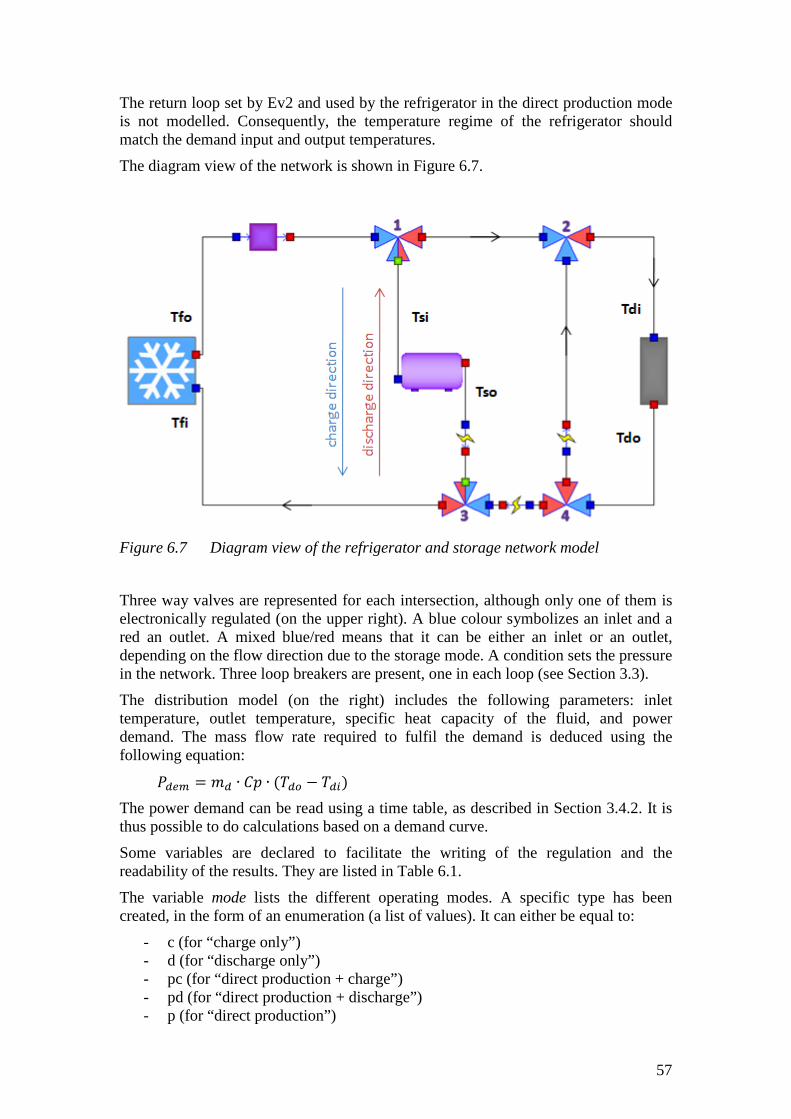
57

The return loop set by Ev2 and used by the refrigerator in the direct production mode is not modelled. Consequently, the temperature regime of the refrigerator should match the demand input and output temperatures.

The diagram view of the network is shown in Figure 6.7.

Figure 6.7 Diagram view of the refrigerator and storage network model

Three way valves are represented for each intersection, although only one of them is electronically regulated (on the upper right). A blue colour symbolizes an inlet and a red an outlet. A mixed blue/red means that it can be either an inlet or an outlet, depending on the flow direction due to the storage mode. A condition sets the pressure in the network. Three loop breakers are present, one in each loop (see Section 3.3).

The distribution model (on the right) includes the following parameters: inlet temperature, outlet temperature, specific heat capacity of the fluid, and power demand. The mass flow rate required to fulfil the demand is deduced using the following equation: �GD= 4 �G ∙ �� ∙ (�GA − �G:) The power demand can be read using a time table, as described in Section 3.4.2. It is thus possible to do calculations based on a demand curve.

Some variables are declared to facilitate the writing of the regulation and the readability of the results. They are listed in Table 6.1.

The variable mode lists the different operating modes. A specific type has been created, in the form of an enumeration (a list of values). It can either be equal to:

- c (for “charge only”) - d (for “discharge only”) - pc (for “direct production + charge”) - pd (for “direct production + discharge”) - p (for “direct production”)

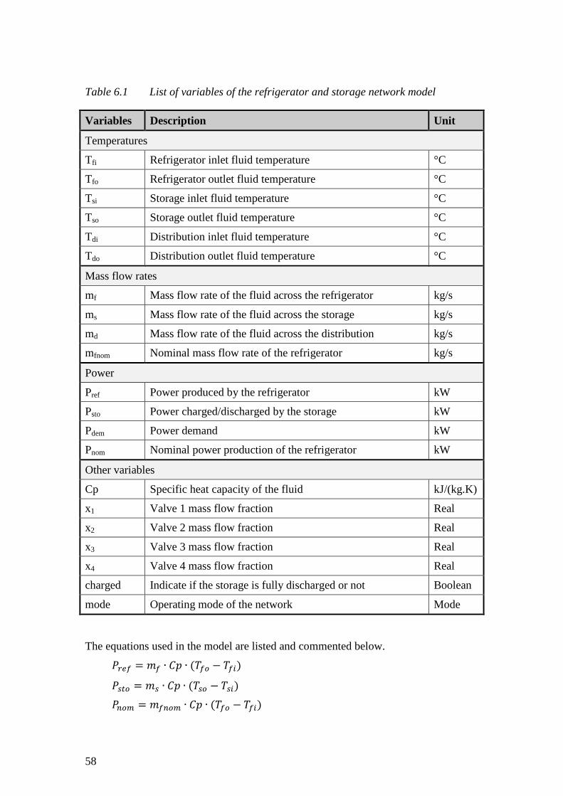
58

Table 6.1 List of variables of the refrigerator and storage network model

Variables Description Unit

Temperatures

Tfi Refrigerator inlet fluid temperature °C

Tfo Refrigerator outlet fluid temperature °C

Tsi Storage inlet fluid temperature °C

Tso Storage outlet fluid temperature °C

Tdi Distribution inlet fluid temperature °C

Tdo Distribution outlet fluid temperature °C

Mass flow rates

mf Mass flow rate of the fluid across the refrigerator kg/s

ms Mass flow rate of the fluid across the storage kg/s

md Mass flow rate of the fluid across the distribution kg/s

mfnom Nominal mass flow rate of the refrigerator kg/s

Power

Pref Power produced by the refrigerator kW

Psto Power charged/discharged by the storage kW

Pdem Power demand kW

Pnom Nominal power production of the refrigerator kW

Other variables

Cp Specific heat capacity of the fluid kJ/(kg.K)

x1 Valve 1 mass flow fraction Real

x2 Valve 2 mass flow fraction Real

x3 Valve 3 mass flow fraction Real

x4 Valve 4 mass flow fraction Real

charged Indicate if the storage is fully discharged or not Boolean

mode Operating mode of the network Mode

The equations used in the model are listed and commented below. �WD� 4 �� ∙ �� ∙ (��A − ��:) �9PA = �9 ∙ �� ∙ (�9A − �9:) �FA= = ��FA= ∙ �� ∙ (��A − ��:)

59

In the model developed, mfnom is declared as a parameter but it can be optimized according to the demand and the storage capacity to avoid over-nominal regimes for the refrigerator.

Valves with 2 inlets and 1 outlet contain the following equations: � ∙ �:6 + (1 − �) ∙ �:5 = �A �:6 = � ∙ �A �:5 = (1 − �) ∙ �A

where i1 is the first inlet, i2 the second inlet, and o the outlet.

Valves with 1 inlet and 2 outlets contain the following equations: �A6 = �: �A5 = �: �A6 = � ∙ �: �A5 = (1 − �) ∙ �: where i is the inlet, o1 the first inlet, and o2 the second outlet.

The mixed valves alternate these equations depending on the storage mode. The second inlet/outlet is always the one vertical in the diagram view of Figure 6.7 (connecting valve 1 to valve 3 and valve 2 to valve 4).

The valves are regulated as follows: �6 = �� �5 = �� The value of the Boolean charged is related to the energy stored in the tank:

+ℎ'�,�� = � ����if��-�',�. �9PAWDG > 0'/��else y Depending on the operating mode, the following variables are assigned:

��-�',�. +ℎ'�,� = � ����if�-�� == +or�+(or�)'/��if�-�� == �or�� y �� = ���FA=if�-�� == +or�+or���Gif�-�� == �0if�-�� == � y ��A = ���A,E>KWCDif�-�� == +or�+�G:if�-�� == �or��or�y

where Tfo,charge is the outlet temperature of the refrigerator during charge regime (declared as a parameter).

The remaining equation selects the current operating mode depending on the power demand Pdem and on the energy left in the storage. For instance:

�-�� = � +if�GD= ≤ 0�if0 < �GD= ≤ �FA=��if�GD= > �FA=and+ℎ'�,�� = �����if�GD= > �FA=and+ℎ'�,�� = '/��y

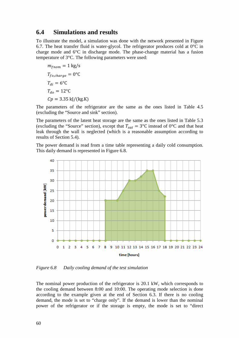
60

6.4 Simulations and results To illustrate the model, a simulation was done with the network presented in Figure 6.7. The heat transfer fluid is water-glycol. The refrigerator produces cold at 0°C in charge mode and 6°C in discharge mode. The phase-change material has a fusion temperature of 3°C. The following parameters were used: ��FA= 4 1kg/s ��A,E>KWCD = 0°C �G: = 6°C �GA = 12°C �� = 3.35kJ/(kg.K) The parameters of the refrigerator are the same as the ones listed in Table 4.5 (excluding the “Source and sink” section).

The parameters of the latent heat storage are the same as the ones listed in Table 5.3 (excluding the “Source” section), except that �9KP = 3°C instead of 0°C and that heat leak through the wall is neglected (which is a reasonable assumption according to results of Section 5.4).

The power demand is read from a time table representing a daily cold consumption. This daily demand is represented in Figure 6.8.

Figure 6.8 Daily cooling demand of the test simulation

The nominal power production of the refrigerator is 20.1 kW, which corresponds to the cooling demand between 8:00 and 10:00. The operating mode selection is done according to the example given at the end of Section 6.3. If there is no cooling demand, the mode is set to “charge only”. If the demand is lower than the nominal power of the refrigerator or if the storage is empty, the mode is set to “direct

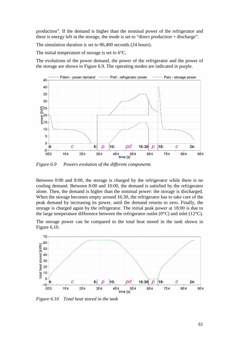
production”. If the demand is higher than the nominal power of the refrigerator and there is energy left in the storage, the mode is set

The simulation duration is set to 86,400 seconds (24 hours).

The initial temperature of storage is set to 6°C.

The evolutions of the power demand, the power of the refrigerator and the power of the storage are shown in Figure 6.9.

Figure 6.9 Powers evolution

Between 0:00 and 8:00, the storage is charged by the refrigerator while there is no cooling demand. Between 8alone. Then, the demand is higher than the nominal power: the storage is discharged. When the storage becomes emptypeak demand by increasing its power, until the demand rstorage is charged again by the refrigerator.the large temperature difference between the refrigerator out

The storage power can be compared to the total heaFigure 6.10.

Figure 6.10 Total heat stored in the tank

production”. If the demand is higher than the nominal power of the refrigerator and there is energy left in the storage, the mode is set to “direct production + discharge”.

The simulation duration is set to 86,400 seconds (24 hours).

The initial temperature of storage is set to 6°C.

The evolutions of the power demand, the power of the refrigerator and the power of Figure 6.9. The operating modes are indicated in purple.

Powers evolution of the different components

, the storage is charged by the refrigerator while there is no cooling demand. Between 8:00 and 10:00, the demand is satisfied by the refrigerator alone. Then, the demand is higher than the nominal power: the storage is discharged. When the storage becomes empty around 16:30, the refrigerator has to take care of the peak demand by increasing its power, until the demand returns to zero. Finally, the storage is charged again by the refrigerator. The initial peak power at 18the large temperature difference between the refrigerator outlet (0°C) and in

The storage power can be compared to the total heat stored in the tank shown in

Total heat stored in the tank

61

production”. If the demand is higher than the nominal power of the refrigerator and to “direct production + discharge”.

The evolutions of the power demand, the power of the refrigerator and the power of The operating modes are indicated in purple.

, the storage is charged by the refrigerator while there is no satisfied by the refrigerator

alone. Then, the demand is higher than the nominal power: the storage is discharged. , the refrigerator has to take care of the

eturns to zero. Finally, the The initial peak power at 18:00 is due to

(0°C) and inlet (12°C).

t stored in the tank shown in

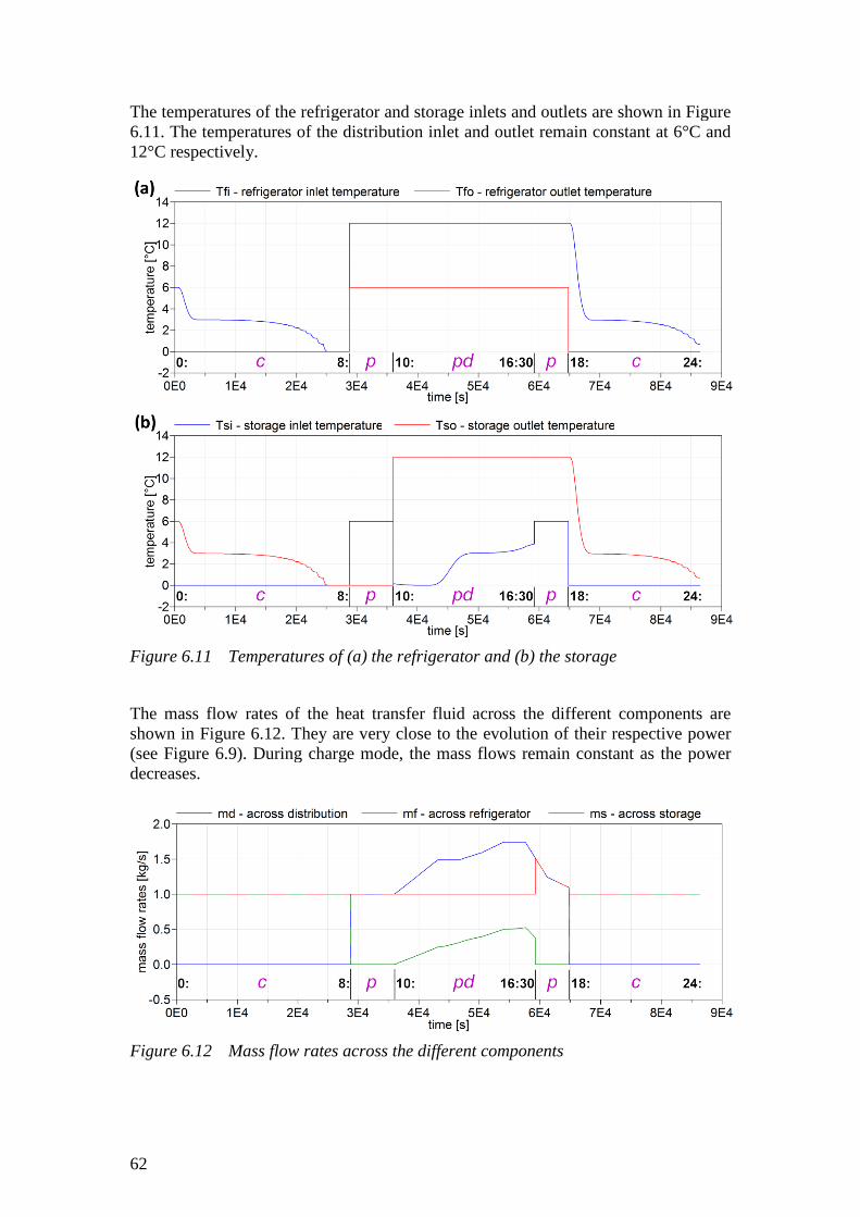
62

The temperatures of the refrigerator and storage inlets and outlets are shown in Figure 6.11. The temperatures of the distr12°C respectively.

Figure 6.11 Temperatures of (a) the refrigerator and (b) the storage

The mass flow rates of the heat transfer fluid across the different components shown in Figure 6.12. They are very close to the evolution of their respective power (see Figure 6.9). During charge mode, the mass flows remain constant as the power decreases.

Figure 6.12 Mass flow rates across the different components

The temperatures of the refrigerator and storage inlets and outlets are shown in Figure The temperatures of the distribution inlet and outlet remain constant at

Temperatures of (a) the refrigerator and (b) the storage

of the heat transfer fluid across the different components They are very close to the evolution of their respective power

During charge mode, the mass flows remain constant as the power

Mass flow rates across the different components

The temperatures of the refrigerator and storage inlets and outlets are shown in Figure ibution inlet and outlet remain constant at 6°C and

of the heat transfer fluid across the different components are They are very close to the evolution of their respective power

During charge mode, the mass flows remain constant as the power

63

Other test simulations have been run with alternative cooling demands and regulations. It has been observed that the Modelica/Dymola environment does not handle very well discontinuities in temperatures and mass flow rates that occur when the operating mode changes. Depending on how the refrigerator regimes and the regulation are set, the simulation may terminate prematurely. This needs further investigation related to the Modelica language itself.

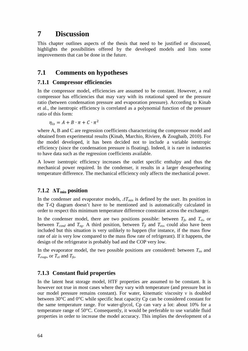
64

7 Discussion This chapter outlines aspects of the thesis that need to be justified or discussed, highlights the possibilities offered by the developed models and lists some improvements that can be done in the future.

7.1 Comments on hypotheses 7.1.1 Compressor efficiencies In the compressor model, efficiencies are assumed to be constant. However, a real compressor has efficiencies that may vary with its rotational speed or the pressure ratio (between condensation pressure and evaporation pressure). According to Kinab et al., the isentropic efficiency is correlated as a polynomial function of the pressure ratio of this form: �:9 4 � H ¥ ∙ + � ∙ 5

where A, B and C are regression coefficients characterizing the compressor model and obtained from experimental results (Kinab, Marchio, Riviere, & Zoughaib, 2010). For the model developed, it has been decided not to include a variable isentropic efficiency (since the condensation pressure is floating). Indeed, it is rare in industries to have data such as the regression coefficients available.

A lower isentropic efficiency increases the outlet specific enthalpy and thus the mechanical power required. In the condenser, it results in a larger desuperheating temperature difference. The mechanical efficiency only affects the mechanical power.

7.1.2 ∆Tmin position In the condenser and evaporator models, ∆Tmin is defined by the user. Its position in the T-Q diagram doesn’t have to be mentioned and is automatically calculated in order to respect this minimum temperature difference constraint across the exchanger.

In the condenser model, there are two positions possible: between Tfo and Tei, or between Tcond and Teg. A third position, between Tfi and Teo, could also have been included but this situation is very unlikely to happen (for instance, if the mass flow rate of air is very low compared to the mass flow rate of refrigerant). If it happens, the design of the refrigerator is probably bad and the COP very low.

In the evaporator model, the two possible positions are considered: between Teo and Tevap, or Tei and Tfo.

7.1.3 Constant fluid properties In the latent heat storage model, HTF properties are assumed to be constant. It is however not true in most cases where they vary with temperature (and pressure but in our model pressure remains constant). For water, kinematic viscosity ν is doubled between 30°C and 0°C while specific heat capacity Cp can be considered constant for the same temperature range. For water-glycol, Cp can vary a lot: about 10% for a temperature range of 50°C. Consequently, it would be preferable to use variable fluid properties in order to increase the model accuracy. This implies the development of a

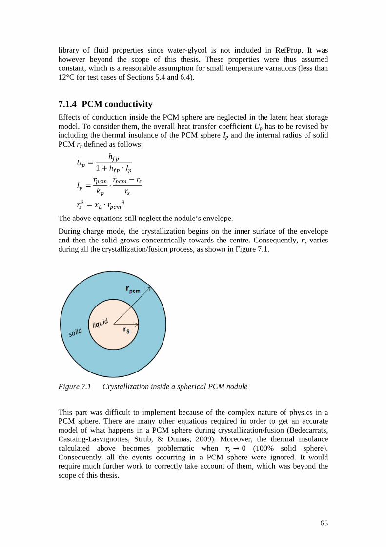
library of fluid properties since waterhowever beyond the scope of constant, which is a reasonable assumption for small temperature 12°C for test cases of Sections 5.4 and 6.4)

7.1.4 PCM conductivityEffects of conduction inside the PCM sphere are neglectedmodel. To consider them, the overall heat transfer coefficient including the thermal insulance of the PCM sphere PCM rs defined as follows:

�L 4 �L1 H �L ∙ ¦L

¦L 4 �LE=�L ∙ �LE= ; �9�9�9� 4 �� ∙ �LE=� The above equations still neglect the nodule’s envelope.

During charge mode, the crystallization begins on the inner surface of the envelope and then the solid grows concentrically towards the centre. Conduring all the crystallization/fusion process, as shown in Figure 7.1.

Figure 7.1 Crystallization inside a spherical PCM nodule

This part was difficult to implement because PCM sphere. There are many other equations required in order to get an accurate model of what happens in a PCM sphere during crystallization/fusionCastaing-Lasvignottes, Strub, & Dumas, 2009)calculated above becomes problematic whenConsequently, all the events occurringrequire much further work to correctly take accountscope of this thesis.

library of fluid properties since water-glycol is not included in RefPropthe scope of this thesis. These properties were thus assumed

constant, which is a reasonable assumption for small temperature variations (less than 12°C for test cases of Sections 5.4 and 6.4).

PCM conductivity Effects of conduction inside the PCM sphere are neglected in the latent heat storage

To consider them, the overall heat transfer coefficient Up has to be revised including the thermal insulance of the PCM sphere Ip and the internal radius of solid

as follows:

�9

The above equations still neglect the nodule’s envelope.

During charge mode, the crystallization begins on the inner surface of the envelope and then the solid grows concentrically towards the centre. Consequently, during all the crystallization/fusion process, as shown in Figure 7.1.

Crystallization inside a spherical PCM nodule

This part was difficult to implement because of the complex nature of physics in a are many other equations required in order to get an accurate

model of what happens in a PCM sphere during crystallization/fusionLasvignottes, Strub, & Dumas, 2009). Moreover, the thermal insulance

lated above becomes problematic when �9 → 0 (100% solid sphere). all the events occurring in a PCM sphere were ignored.

further work to correctly take account of them, which was beyond the

65

glycol is not included in RefProp. It was . These properties were thus assumed

variations (less than

in the latent heat storage has to be revised by

and the internal radius of solid

During charge mode, the crystallization begins on the inner surface of the envelope sequently, rs varies

of the complex nature of physics in a are many other equations required in order to get an accurate

model of what happens in a PCM sphere during crystallization/fusion (Bedecarrats, Moreover, the thermal insulance

(100% solid sphere). ignored. It would

, which was beyond the

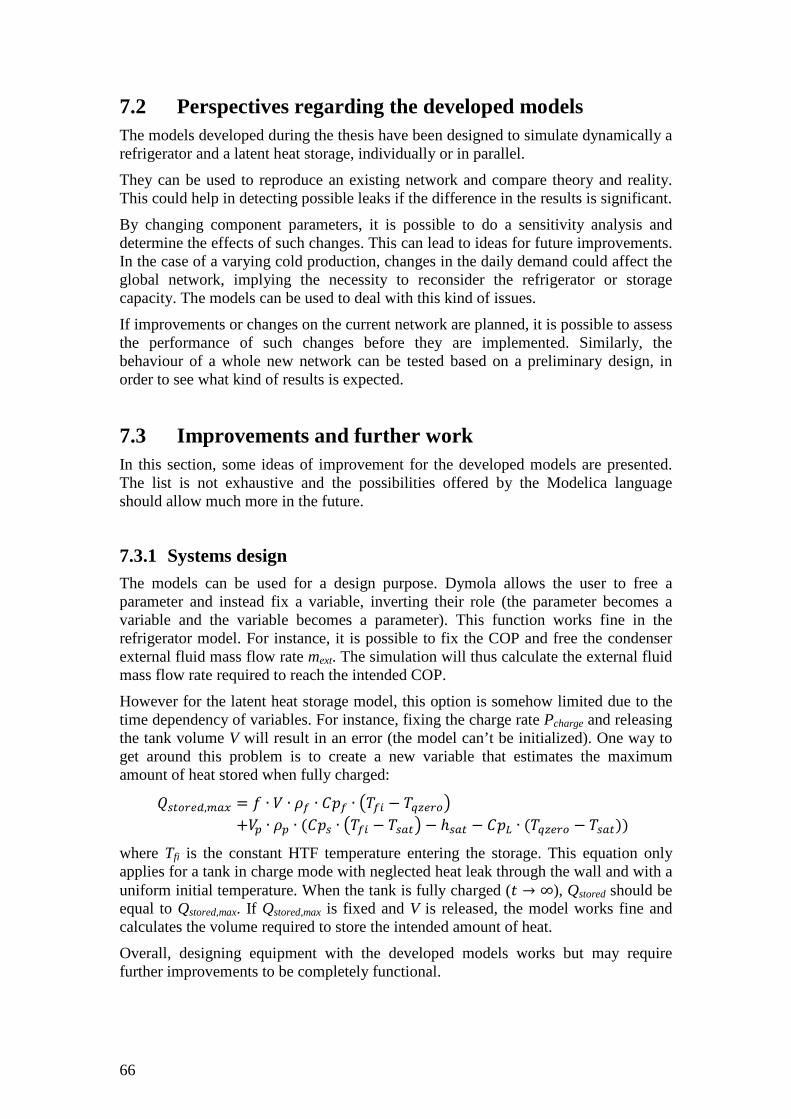
66

7.2 Perspectives regarding the developed models The models developed during the thesis have been designed to simulate dynamically a refrigerator and a latent heat storage, individually or in parallel.

They can be used to reproduce an existing network and compare theory and reality. This could help in detecting possible leaks if the difference in the results is significant.

By changing component parameters, it is possible to do a sensitivity analysis and determine the effects of such changes. This can lead to ideas for future improvements. In the case of a varying cold production, changes in the daily demand could affect the global network, implying the necessity to reconsider the refrigerator or storage capacity. The models can be used to deal with this kind of issues.

If improvements or changes on the current network are planned, it is possible to assess the performance of such changes before they are implemented. Similarly, the behaviour of a whole new network can be tested based on a preliminary design, in order to see what kind of results is expected.

7.3 Improvements and further work In this section, some ideas of improvement for the developed models are presented. The list is not exhaustive and the possibilities offered by the Modelica language should allow much more in the future.

7.3.1 Systems design The models can be used for a design purpose. Dymola allows the user to free a parameter and instead fix a variable, inverting their role (the parameter becomes a variable and the variable becomes a parameter). This function works fine in the refrigerator model. For instance, it is possible to fix the COP and free the condenser external fluid mass flow rate mext. The simulation will thus calculate the external fluid mass flow rate required to reach the intended COP.

However for the latent heat storage model, this option is somehow limited due to the time dependency of variables. For instance, fixing the charge rate Pcharge and releasing the tank volume V will result in an error (the model can’t be initialized). One way to get around this problem is to create a new variable that estimates the maximum amount of heat stored when fully charged: �9PAWDG,=K? = ∙ � ∙ !� ∙ ��� ∙ @��: − ���DWAB

+�L ∙ !L ∙ (��9 ∙ @��: − �9KPB − ℎ9KP − ��� ∙ (���DWA − �9KP))

where Tfi is the constant HTF temperature entering the storage. This equation only applies for a tank in charge mode with neglected heat leak through the wall and with a uniform initial temperature. When the tank is fully charged (� → ∞), Qstored should be equal to Qstored,max. If Qstored,max is fixed and V is released, the model works fine and calculates the volume required to store the intended amount of heat.

Overall, designing equipment with the developed models works but may require further improvements to be completely functional.

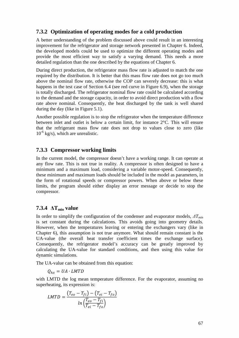
67

7.3.2 Optimization of operating modes for a cold production A better understanding of the problem discussed above could result in an interesting improvement for the refrigerator and storage network presented in Chapter 6. Indeed, the developed models could be used to optimize the different operating modes and provide the most efficient way to satisfy a varying demand. This needs a more detailed regulation than the one described by the equations of Chapter 6.

During direct production, the refrigerator mass flow rate is adjusted to match the one required by the distribution. It is better that this mass flow rate does not go too much above the nominal flow rate, otherwise the COP can severely decrease: this is what happens in the test case of Section 6.4 (see red curve in Figure 6.9), when the storage is totally discharged. The refrigerator nominal flow rate could be calculated according to the demand and the storage capacity, in order to avoid direct production with a flow rate above nominal. Consequently, the heat discharged by the tank is well shared during the day (like in Figure 5.1).

Another possible regulation is to stop the refrigerator when the temperature difference between inlet and outlet is below a certain limit, for instance 2°C. This will ensure that the refrigerant mass flow rate does not drop to values close to zero (like 10-6 kg/s), which are unrealistic.

7.3.3 Compressor working limits In the current model, the compressor doesn’t have a working range. It can operate at any flow rate. This is not true in reality. A compressor is often designed to have a minimum and a maximum load, considering a variable motor-speed. Consequently, these minimum and maximum loads should be included in the model as parameters, in the form of rotational speeds or compressor powers. When above or below these limits, the program should either display an error message or decide to stop the compressor.

7.3.4 ∆Tmin value In order to simplify the configuration of the condenser and evaporator models, ∆Tmin is set constant during the calculations. This avoids going into geometry details. However, when the temperatures leaving or entering the exchangers vary (like in Chapter 6), this assumption is not true anymore. What should remain constant is the UA-value (the overall heat transfer coefficient times the exchange surface). Consequently, the refrigerator model’s accuracy can be greatly improved by calculating the UA-value for standard conditions, and then using this value for dynamic simulations.

The UA-value can be obtained from this equation: �>? 4 �� ∙ ©��

with LMTD the log mean temperature difference. For the evaporator, assuming no superheating, its expression is:

©�� = @�DA − ��:B − @�D: − ��AB/� ��DA − ��:

�D: − ��A�

68

7.3.5 Temperature inertia In the refrigerator and storage network, the switch between charge and discharge regime causes discontinuities in temperatures, as shown in Figure 6.11. In reality, when a valve opens or closes, there is inertia before the new temperature is reached. A ramp could be generated to avoid these discontinuities and give a more accurate result. Additionally, the refrigerator model could include temperature-time integrals to make the system even more dynamic.

69

8 Conclusion This thesis has demonstrated the potential offered by the Modelica language for developing models of industrial energy technologies, in order to make dynamic simulations. Based on equations instead of assignment statements, its acausality simplifies the programming and extends the ways a model can be used. Combined to the Dymola environment, the user can easily create, assemble and configure models thanks to an advanced graphical user interface.

The models developed during this thesis were designed to take advantage of these benefits. They gather technologies related to cold production and storage: refrigerator, combined refrigerator/heat pump, and latent heat storage. Each of them can be used individually or in parallel with other systems. To guarantee their compatibility in any case, some additional components such as loop breakers were developed.

Beyond the physical study of the technologies, a part of the thesis was focused on the development of a library of refrigerant properties. On one hand, using the RefProp database offers an extensive amount of fluids but it limits future distribution of the models. On the other hand, using polynomial functions gives fast but less accurate results, while requiring much more work to be exhaustive. Both solutions have their qualities and will probably need improvements in the future.

If they are in some way limited by the hypotheses taken, the models give results which are very close to what is expected in reality. The values calculated by the refrigerator model differ from experimental values by only a few percents, delivering a reasonable accuracy. The latent heat storage has not been tested experimentally but the results obtained concur with the literature from where the mathematical model is extracted.

One way to combine the models developed is to conceive a network with a refrigerator and a latent heat storage, which distributes cold according to a varying demand and regulation equations. This rather complex assembling seems to work fine when the regulation is carefully defined, although it is not flawless in some cases. Such modelling offers great possibilities for reproducing the behaviour of different operating modes and how they switch according to the cooling demand.

Applications for the developed models are numerous and range from simple comparisons of theory and reality to sensitivity analysis on parameters and performance assessments of future systems or improvements. Additionally, the models can be used to design systems by permuting a variable and a parameter. For instance, it is possible to optimize the COP of a refrigerator or calculate the required volume storage for a specific demand.

To conclude, the models developed during the thesis offers a wide range of parameters and applications that can be of great help for industries which want to study and improve the efficiency of their systems. The results obtained give in most cases a good accuracy, although there is still room for improvement. This is all the more true as the Modelica language will continue to evolve in the future.

70

9 References Assaf, K. (2010). Intégration d'une pompe à chaleur dans un procédé

agroalimentaire - Simulation, expérimentation et intégration. Ph.D. Thesis.

Beasley, D. E., & Clark, J. A. (1984). Transient response of a packed bed for thermal energy storage. International Journal of Heat and Mass Transfer , Vol. 27 (No. 9), pp. 1659-1669.

Bedecarrats, J. P., Castaing-Lasvignottes, J., Strub, F., & Dumas, J. (2009). Study of a phase change energy storage using spherical capsules. Part II: Numerical modelling. Energy Conversion and Management , Vol. 50 (No. 10), pp. 2537-2546.

Bouskela, D. (2003). Bibliothèque Modelica thermohydraulique, structure et recommandations de conception. EDF R&D.

Cellier, F. (2005). Dymola: Environment for Object-oriented Modeling of Physical Systems. Retrieved July 5, 2011, from ETH Zürich: http://www.inf.ethz.ch/personal/fcellier/Res/Soft/Dymola_engl.html

Cleland, A. C. (1992). Polynomial curve-fits for refrigerant thermodynamic properties: extension to include R134a. International Journal of Refrigeration , Vol. 17 (No. 4), pp. 245-249.

Cristopia. (2008). Cristopia STL Brochure. Retrieved from Cristopia Energy Systems: http://www.cristopia.com/

Dassault Systèmes. (2010). Customer Testimonies on Industry and Mid-market PLM and 3D Simulation Solutions. Retrieved July 5, 2011, from 3DS: http://www.3ds.com/company/customer-stories/

Dehon. (2007). Neutragel Neo brochure. Retrieved from Neutragel: http://www.climalife.dehon.com/uploads/media/3/356/356_1205_neutragel-neo-pds-en.pdf

Galloway, T. R., & Sage, B. H. (1970). A model of the mechanism of transport in packed, distended, and fluidized beds. Chemical Engineering Science , Vol. 25 (No. 3), pp. 495-516.

Hausen, H. (1959). Neue Gleichungen für die Wärmeübertragung bei freier und erzwungener Strömung. Allg. Wärmetechnik , Vol. 9, pp.75-79.

Kinab, E., Marchio, D., Riviere, P., & Zoughaib, A. (2010). Reversible heat pump model for seasonal performance optimization. Energy and Buildings , Vol. 42 (No. 12), pp. 2269-2280.

Lemmon, E. W., McLinden, M. O., & Huber, M. L. (2007). RefProp: NIST Reference Fluid Thermodynamic and Transport Properties, Version 8.0. National Institute of Standards and Technology, Gaithersburg.

Li, Z., Zheng, L., & Zhang, H. (2008). Solving PDE Models in Modelica. International Symposium on Information Science and Engineering , Vol. 1, pp. 53-57.

Mehling, H., & Cabeza, L. (2008). Heat and cold storage with PCM: an up to date introduction into basics and applications. Springer.

Modelica Association. (2010). Modelica Language Specification - Version 3.2.

71

Regin, A. F., Solanki, S. C., & Saini, J. S. (2008). Heat transfer characteristics of thermal energy storage system using PCM capsules: A review. Renewable and Sustainable Energy Reviews , Vol. 12 (No. 9), pp. 2438-2458.

TLK-Thermo GmbH. (2009). TIL - Modelica Library for Simulation of Fluid Systems. Retrieved July 24, 2011, from TLK-Thermo GmbH: http://www.tlk-thermo.com/

Wu, S., Fang, G., & Liu, X. (2011). Dynamic discharging characteristics simulation on solar heat storage system with spherical capsules using paraffin as heat storage material. Renewable Energy , Vol. 36 (No. 4), pp. 1190-1195.

Young, H. D. (1992). University Physics, 7th Ed. Addison Weasley.

72

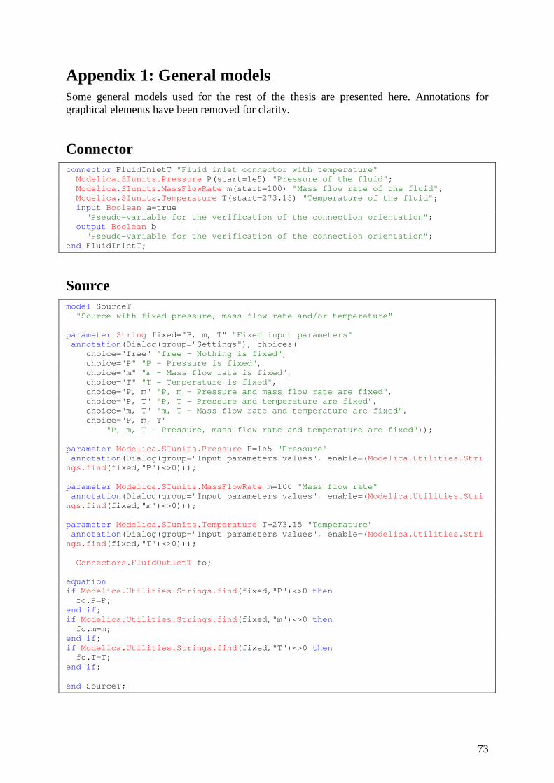
73

Appendix 1: General models Some general models used for the rest of the thesis are presented here. Annotations for graphical elements have been removed for clarity.

Connector connector FluidInletT "Fluid inlet connector with temperature" Modelica.SIunits.Pressure P(start=1e5) "Pressure of the fluid"; Modelica.SIunits.MassFlowRate m(start=100) "Mass flow rate of the fluid"; Modelica.SIunits.Temperature T(start=273.15) "Temperature of the fluid"; input Boolean a=true "Pseudo-variable for the verification of the connection orientation"; output Boolean b "Pseudo-variable for the verification of the connection orientation"; end FluidInletT;

Source model SourceT "Source with fixed pressure, mass flow rate and/or temperature" parameter String fixed="P, m, T" "Fixed input parameters" annotation(Dialog(group="Settings"), choices( choice="free" "free - Nothing is fixed", choice="P" "P - Pressure is fixed", choice="m" "m - Mass flow rate is fixed", choice="T" "T - Temperature is fixed", choice="P, m" "P, m - Pressure and mass flow rate are fixed", choice="P, T" "P, T - Pressure and temperature are fixed", choice="m, T" "m, T - Mass flow rate and temperature are fixed", choice="P, m, T" "P, m, T - Pressure, mass flow rate and temperature are fixed")); parameter Modelica.SIunits.Pressure P=1e5 "Pressure" annotation(Dialog(group="Input parameters values", enable=(Modelica.Utilities.Strings.find(fixed,"P")<>0))); parameter Modelica.SIunits.MassFlowRate m=100 "Mass flow rate" annotation(Dialog(group="Input parameters values", enable=(Modelica.Utilities.Strings.find(fixed,"m")<>0))); parameter Modelica.SIunits.Temperature T=273.15 "Temperature" annotation(Dialog(group="Input parameters values", enable=(Modelica.Utilities.Strings.find(fixed,"T")<>0))); Connectors.FluidOutletT fo; equation if Modelica.Utilities.Strings.find(fixed,"P")<>0 then fo.P=P; end if; if Modelica.Utilities.Strings.find(fixed,"m")<>0 then fo.m=m; end if; if Modelica.Utilities.Strings.find(fixed,"T")<>0 then fo.T=T; end if; end SourceT;

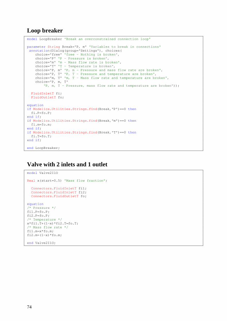
74

Loop breaker model LoopBreaker "Break an overconstrained connection loop" parameter String Break="P, m" "Variables to break in connections" annotation(Dialog(group="Settings"), choices( choice="free" "free - Nothing is broken", choice="P" "P - Pressure is broken", choice="m" "m - Mass flow rate is broken", choice="T" "T - Temperature is broken", choice="P, m" "P, m - Pressure and mass flow rate are broken", choice="P, T" "P, T - Pressure and temperature are broken", choice="m, T" "m, T - Mass flow rate and temperature are broken", choice="P, m, T" "P, m, T - Pressure, mass flow rate and temperature are broken")); FluidInletT fi; FluidOutletT fo; equation if Modelica.Utilities.Strings.find(Break,"P")==0 then fi.P=fo.P; end if; if Modelica.Utilities.Strings.find(Break,"m")==0 then fi.m=fo.m; end if; if Modelica.Utilities.Strings.find(Break,"T")==0 then fi.T=fo.T; end if; end LoopBreaker;

Valve with 2 inlets and 1 outlet model Valve2I1O Real x(start=0.5) "Mass flow fraction"; Connectors.FluidInletT fi1; Connectors.FluidInletT fi2; Connectors.FluidOutletT fo; equation /* Pressure */ fi1.P=fo.P; fi2.P=fo.P; /* Temperature */ x*fi1.T+(1-x)*fi2.T=fo.T; /* Mass flow rate */ fi1.m=x*fo.m; fi2.m=(1-x)*fo.m; end Valve2I1O;

75

Appendix 2: Refrigerator Modelica models

Compressor Confidential and property of EDF R&D.

Condenser Confidential and property of EDF R&D.

Evaporator Confidential and property of EDF R&D.

Expansion valve Confidential and property of EDF R&D.

Refrigerator Confidential and property of EDF R&D.

Combined refrigerator/heat pump Confidential and property of EDF R&D.

76

Appendix 3: Storage Modelica models Confidential and property of EDF R&D.