Embed Size (px)
Citation preview
Journal of Machine Learning Research 4 (2003) 39-66 Submitted 3/02; Revised 10/02; Published 4/03
Designing Committees of Models through Deliberate Weighting ofData Points
Stefan W. Christensen [email protected]
Department of ChemistryUniversity of SouthamptonSouthampton, SO17 1BJ, UK
Ian Sinclair [email protected]
Philippa A. S. Reed [email protected]
Materials Research GroupSchool of Engineering SciencesUniversity of SouthamptonSouthampton, SO17 1BJ, UK
Editor: Thomas G. Dietterich
AbstractIn the adaptive derivation of mathematical models from data, each data point should contribute witha weight reflecting the amount of confidence one has in it. When no additional information for dataconfidence is available, all the data points should be considered equal, and are also generally giventhe same weight. In the formation of committees of models, however, this is often not the case andthe data points may exercise unequal, even random, influence over the committee formation.
In this paper, a principled approach to committee design is presented. The construction of acommittee design matrix is detailed through which each data point will contribute to the committeeformation with a fixed weight, while contributing with different individual weights to the derivationof the different constituent models, thus encouraging model diversity whilst not biasing the com-mittee inadvertently towards any particular data points. Not distinctly an algorithm, it is instead aframework within which several different committee approaches may be realised.
Whereas the focus in the paper lies entirely on regression, the principles discussed extendreadily to classification.Keywords: Neural Networks, Ensembles, Committees, Bagging
1. Introduction
Identifying the true structure of a system via modelling is, in general, not an easy task. Any modelwill be limited in complexity and though ideally this will match that of the system exactly, in realityit rarely will. Obtaining a model amounts to choosing between two evils: reduce the complexity toomuch, and the model fails to duplicate the finer aspects of the system; allow too much flexibility,and the model introduces spurious aspects, overfitting the data.
Typically, this is addressed via regularisation, which allows the complexity to be adjusted. Un-fortunately however, the architecture of the model may not be commensurate with the system, inwhich case no amount of regularisation will yield the perfect model. Moreover, even if the archi-tecture is correct, the modelling may fail to provide the globally optimal model, instead settling fora locally optimal one.
c©2003 Stefan W. Christensen, Ian Sinclair and Philippa A. S. Reed.
CHRISTENSEN, SINCLAIR AND REED
An alternative approach is to establish a committee of models, with two main approaches nor-mally being distinguished: ensemble- and modular techniques. In the case of ensembles (Hansenand Salamon, 1990), the predictions of a number of individual models are averaged. The expec-tation being that where some models will overshoot the target, others will predict too low a value,and so the ensemble prediction will be more accurate than the predictions of the individual modelsare on average. This has been established by Krogh and Vedelsby (1995). In the case of modularapproaches, e.g. mixtures of experts (Jacobs et al., 1991), a number of individual models, each ex-pected to be particularly accurate in certain respects but less so in others, complement one anotherso that their combination, via a gating network, may attain a high degree of accuracy everywhere.
The typical view of committees is that their prediction error can be decomposed into bias andvariance; a more practical decomposition is that into average error of the constituent models, andtheir ambiguity (Krogh and Vedelsby, 1995). According to the latter, a clear prerequisite for theformation of a successful committee is that the individual models differ significantly from one an-other. In the case of mixtures of experts this is inevitable, by virtue of their definition. In the case ofensembles, it is not. In fact, it may be quite a formidable task to ensure that the individual modelsare not mimicking closely each others behaviour. In basic ensembles, where a straight average istaken over a number of generated models, many of these may be very similar. This problem maybe reduced by weighting the models differently, e.g. by optimising the weights to obtain the low-est possible error (Perrone and Cooper, 1993), by using singular value decomposition to obtain theunique aspects of the models (Mertz, 1998), or by discarding individual models after an investi-gation of model collinearity (Hashem, 1997). Alternatively, models can be generated specificallyto be different,either via encouraging diversity: e.g. bagging (Breiman, 1996), boosting (Shapire,1990), through input feature grouping (Liao and Moody, 2000), or introduction of noise into theoutputs (Breiman, 1998, Raviv and Intrator, 1996) (see e.g. Dietterich, 2000, for an overview ofapproaches),or via strictly enforcing it (Rosen, 1996, Opitz and Shavlik, 1996, Liu and Yao, 1998,1999). The idea introduced in the present paper is closely related to bagging, and it is positionedfirmly within the “encouraging diversity” category.
Following a brief explanatory note on the use of the word “weight”, Section 2 makes the casefor the designed committee and presents the theory. Section 3 concerns a very real problem thatthe approach may entail, and a way to circumvent it. Section 4 shows some practical test results,comparing the designed committee approach and bagging. In Section 5, the method and results arediscussed, and conclusions, finally, are in Section 6.
1.1 A Note on Weights
In this paper, frequent use will be made of the word “weight”. Three separate kinds of weights areto be distinguished; the first of these, the well established “weights” of a neural network, whosefinal determination concludes model optimisation, will not concern us here. The second kind is themodelweights that determine the contribution of the individual models to an ensemble’s prediction.These will be referred to aswm, a vector of as many elements as there are models in the ensemble.
The third (and in this paper central) kind are thedata pointweights that determine the influenceexercised by the individual data points on the model formation (to be referred to viaD, the designmatrix), and on the committee formation (referred to aswp, a vector of as many elements as thereare training data).
40

DESIGNING COMMITTEES OFMODELS THROUGHDELIBERATE WEIGHTING OF DATA POINTS
2. Committee Design1
Whilst the weighting of the individual models has been a central issue in committee based modellingso far, the possibility of weighting the influence of individual data points in a rigorous and deliberatemanner seems to have been somewhat neglected, if not completely untried. One approach, whichdepends intrinsically on such weighting is boosting, via which emphasis is put on certain data pointsthat are observed to be particularly difficult to predict accurately. This makes boosting an adaptivetechnique, i.e. the weighting is a result of the modelling. In the present paper a new, systematicapproach to the formation of committees is proposed, whereby these are formallydesigned, by wayof premeditatedweighting of points.
2.1 Non-egalitarian Weighting Schemes
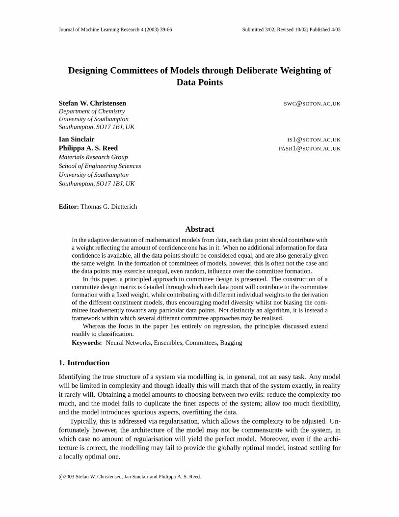
In bagging, or bootstrap aggregating, one of the most popular committee techniques, models areobtained through applying the modelling algorithm several times on data sets, each generated viarandom sampling, with replacement, of N data points from the original training set, also of N datapoints. The models are then combined into a committee, which benefits from the diversity intro-duced by the difference in training data sets. Breiman (1999) argued that “Bagging samples eachinstance with equal probability - it is perfectly democratic.” While it is certainly true that eachdata point is chosen for the training set of a model with equal probability (provided the selectionalgorithm used is truly random) and that from this perspective bagging may be said to be entirelydemocratic, the final committee is unlikely to put equal emphasis on each data point, as all datapoints are unlikely to be chosen for training equally often - unless an infinite (or at least very large)number of models is included in the committee. Or, in other words, the data distribution (over inputspace), seen by the committee, may differ from the empirical distribution, given by the original dataset, if the number of models included is finite. To illustrate the degree to which actual committeesmay emphasise certain data points more than others, a series of bootstrapping experiments has beencarried out here.
What was sought was an understanding of the extent to which the individual data points aregiven equal, or at least similar, weights in the committee, as a function of the number of modelsincluded in it, and as a function of the number of training data. The bootstrap experiment was asfollows:
• For a given number of models per committee, m, and a given number of data points, n, set upthe resampled training sets.
• Count the number of instances of every original data point within these and, in turn, over thewhole committee.
• Calculate, for each data point, the ratio of number of instances to the total number of datapoints in the committee (i.e. m x n). These ratios are the weights of the individual data points;their sum is unity.
• Calculate the relative standard deviation from the mean of these weights (std. dev. divided bythe average weight size), A, and the ratio of the largest weight to the smallest, B.
1. Liao and Moody (2000) suggested a way to generate “designed committees” which, aside from sharing the objectiveof increasing model diversity, is unrelated to the approach presented here.
41
CHRISTENSEN, SINCLAIR AND REED
0.0
0.1
0.2
0.3
0.4
0.5
0.6
0.7
0.8
0.9
1.0
1 10 100 1000
No. of models in committee
Rel
ativ
e st
anda
rd d
evia
tion
201005002500
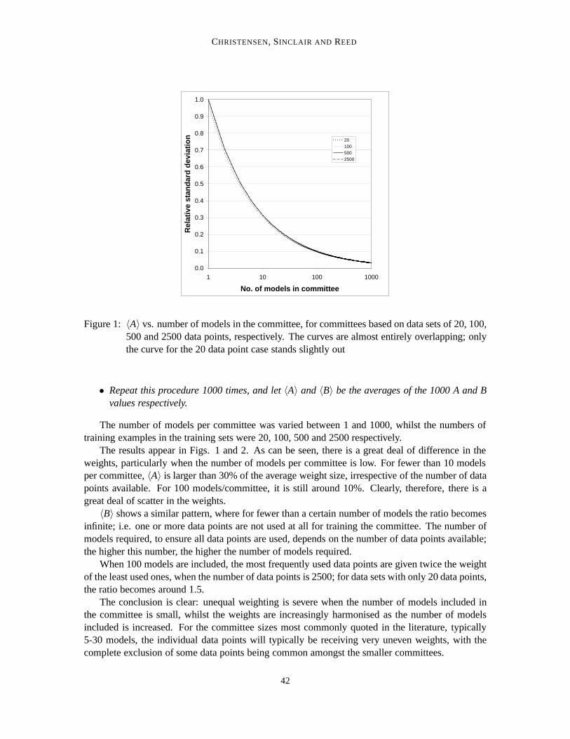
Figure 1: 〈A〉 vs. number of models in the committee, for committees based on data sets of 20, 100,500 and 2500 data points, respectively. The curves are almost entirely overlapping; onlythe curve for the 20 data point case stands slightly out
• Repeat this procedure 1000 times, and let〈A〉 and 〈B〉 be the averages of the 1000 A and Bvalues respectively.
The number of models per committee was varied between 1 and 1000, whilst the numbers oftraining examples in the training sets were 20, 100, 500 and 2500 respectively.
The results appear in Figs. 1 and 2. As can be seen, there is a great deal of difference in theweights, particularly when the number of models per committee is low. For fewer than 10 modelsper committee,〈A〉 is larger than 30% of the average weight size, irrespective of the number of datapoints available. For 100 models/committee, it is still around 10%. Clearly, therefore, there is agreat deal of scatter in the weights.
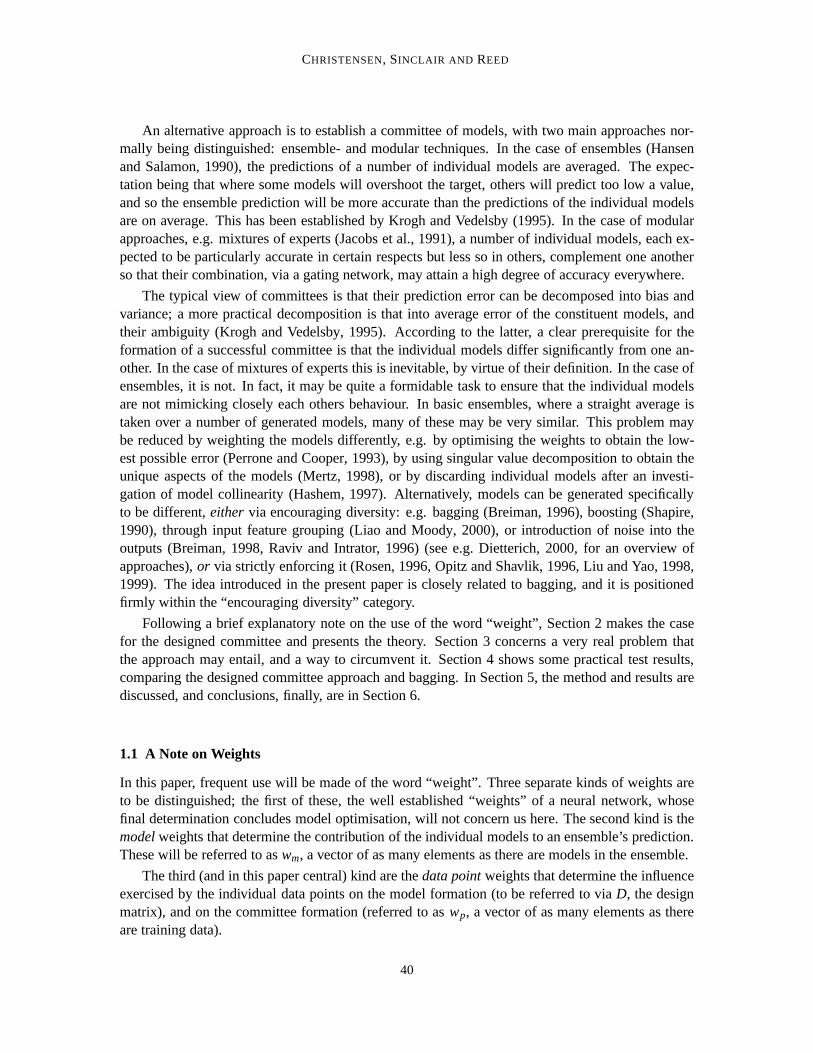
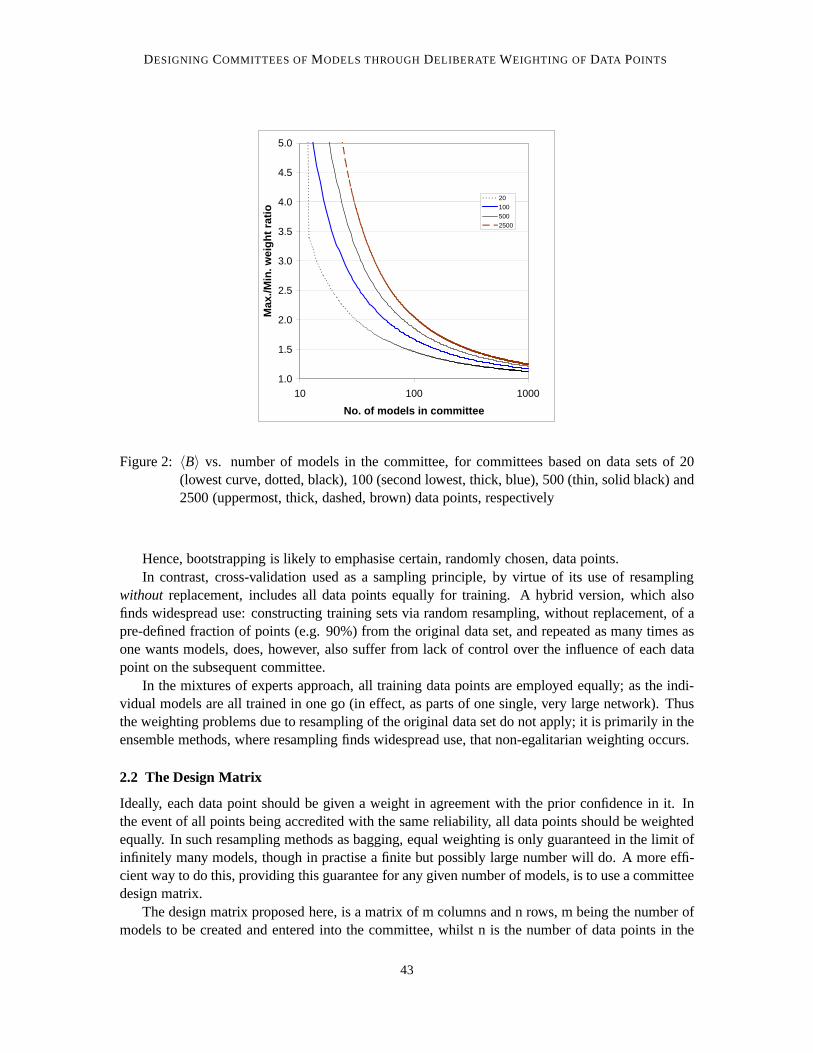
〈B〉 shows a similar pattern, where for fewer than a certain number of models the ratio becomesinfinite; i.e. one or more data points are not used at all for training the committee. The number ofmodels required, to ensure all data points are used, depends on the number of data points available;the higher this number, the higher the number of models required.
When 100 models are included, the most frequently used data points are given twice the weightof the least used ones, when the number of data points is 2500; for data sets with only 20 data points,the ratio becomes around 1.5.
The conclusion is clear: unequal weighting is severe when the number of models included inthe committee is small, whilst the weights are increasingly harmonised as the number of modelsincluded is increased. For the committee sizes most commonly quoted in the literature, typically5-30 models, the individual data points will typically be receiving very uneven weights, with thecomplete exclusion of some data points being common amongst the smaller committees.
42
DESIGNING COMMITTEES OFMODELS THROUGHDELIBERATE WEIGHTING OF DATA POINTS
1.0
1.5
2.0
2.5
3.0
3.5
4.0
4.5
5.0
10 100 1000
No. of models in committee
Max
./Min
. wei
ght r
atio
201005002500
Figure 2: 〈B〉 vs. number of models in the committee, for committees based on data sets of 20(lowest curve, dotted, black), 100 (second lowest, thick, blue), 500 (thin, solid black) and2500 (uppermost, thick, dashed, brown) data points, respectively
Hence, bootstrapping is likely to emphasise certain, randomly chosen, data points.In contrast, cross-validation used as a sampling principle, by virtue of its use of resampling
without replacement, includes all data points equally for training. A hybrid version, which alsofinds widespread use: constructing training sets via random resampling, without replacement, of apre-defined fraction of points (e.g. 90%) from the original data set, and repeated as many times asone wants models, does, however, also suffer from lack of control over the influence of each datapoint on the subsequent committee.
In the mixtures of experts approach, all training data points are employed equally; as the indi-vidual models are all trained in one go (in effect, as parts of one single, very large network). Thusthe weighting problems due to resampling of the original data set do not apply; it is primarily in theensemble methods, where resampling finds widespread use, that non-egalitarian weighting occurs.
2.2 The Design Matrix
Ideally, each data point should be given a weight in agreement with the prior confidence in it. Inthe event of all points being accredited with the same reliability, all data points should be weightedequally. In such resampling methods as bagging, equal weighting is only guaranteed in the limit ofinfinitely many models, though in practise a finite but possibly large number will do. A more effi-cient way to do this, providing this guarantee for any given number of models, is to use a committeedesign matrix.
The design matrix proposed here, is a matrix of m columns and n rows, m being the number ofmodels to be created and entered into the committee, whilst n is the number of data points in the
43

CHRISTENSEN, SINCLAIR AND REED
training set. The elements in the matrix are the weights for the data points, given the specific model;i.e. all weights are within [0,1] and the sum along each column must be unity. To each model isassigned a specific weight (e.g. a weight of 1/m; it must necessarily also reside within [0,1]); thesum of all model weights must come to 1. Finally, and hereby clearly distinguishing committeedesign from bagging, the sum, along every row, of elements multiplied by their respective modelsweight, must equal the overall (i.e. committee) weight for the corresponding data point. In theaforementioned case of all points being treated equally, all such row sums must equal 1/n. In short,
D wm = wp
whereD is the design matrix, withwm andwp being the model weights, and overall (i.e. committee)data point weights.D is subsequently utilised in thetraining of the individual models via weightingthe contributions to the error measure (e.g. the mean squared error, mse) by the correspondingweight fromD; i.e. the error measure becomes:
L j =n
∑i=1
di, j L(yi− f j(xi)) (1)
where j is the index of the model,i is the index of the data point,di, j is the weight from the designmatrix, f j(xi) is the prediction of modelj for data pointi, yi is the true output value for data pointi,andL is the loss function, e.g. the 2-norm; the mean squared error thus becomes aweightedmeansquared error.
Ultimately, when making predictions, the committee is realized through a linear combination ofthe individual models:
ypred, committee = wTm ypred =
m
∑i=1
wmi ypred,i (2)
whereypred,committeeis the predicted output value,ypred is a vector of the individual model predic-tions, andwmi are the model weights.
Bagging committees are, in fact, mathematically extremely similar, and may be realised viathis principle through relaxing the constraint that the row sums come to a predetermined amount;i.e. wp’s elements may take on unequal values between 0 and 1 (specifically, they must take onvalues that are multiples of 1/mn). Boosting committees however, cannot similarly be realised, eventhough boosting shares the aim of controlling the influence of each data point on each model; it isa truly adaptive technique as opposed to the proposed committee design. Interestingly, mixtures ofexperts may be nearly realised through careful construction of the design matrix, e.g. ensuring aspecific model is particularly accurate in certain areas of input space, by weighting the data pointsin those areas higher than those elsewhere; the other models may be similarly designed to focuson other areas of input space. The proposed method of designing committees is therefore a verygeneral approach that may encompass both ensemble and modular techniques.
2.3 Setting up a Design Matrix
A pertinent question, arising when designing a committee of m models using n data points, ishow to set the weights for each data point, so that the individual models will weight different datapoints differently, thus encouraging model diversity, while the committee will weight each data
44

DESIGNING COMMITTEES OFMODELS THROUGHDELIBERATE WEIGHTING OF DATA POINTS
point the same, thereby avoiding biasing the committee towards any particular data points. Clearly,this is a case of solvingn equations withm(n+ 1) unknowns which, asm > 1, has an infinitenumber of solutions. As it is a linear system, these may be sought via Gauss-Jordan, singular valuedecomposition, etc. This may prove costly in terms of computer time and memory, however.
2.3.1 CONSTRUCTING QUASI-BAGGING COMMITTEES
A simple, yet functional way of quickly achieving a “randomised” distribution of weights and, assuch, being close in spirit to bagging, whilst still adhering to the strictly equal weighting of each datapoint overall, is to initially give all m models the same weight (i.e. 1/m) while setting up a designmatrix of equal weights, i.e. all weights,di, j = 1/n and then, repeatedly for randomly chosen 2x2sub matrices from the matrix, make random alterations to 1 of the 4 weights and changing theother 3 so that constant sums along both the 2 rows and the 2 columns are maintained. If repeatedsufficiently, the weights seem to be quite “randomised”.2
Consider this example (Equation 3): there are three data points and 2 models in the committee;i.e. we have a weight matrix with 6 elements, each with the initial weight of 1/3, both models havingthe same weight of 0.5. If a small change is made to e.g. element (1,1), then a similar change mustbe made to the element (1,2) but with opposite sign.3 Also, either element (2,1) or, as chosen here,(3,1) must be changed by the same amount, also with the opposite sign. Finally, the last element,here (3,2), must be changed exactly as was (1,1) in order to maintain the same weight for all threedata points within the committee; i.e. leavingwp undisturbed.
Doriginal =
13
13
13
13
13
13
=⇒ Daltered =
13 + δ 1
3−δ13
13
13−δ 1
3 + δ
(3)
This process is repeated for consecutive 2x2 sub matrices until the weights are adequately “ran-domised”; within the committee each data point will maintain its initial weight throughout.4
2.3.2 CONSTRUCTINGCROSS-VALIDATION COMMITTEES
Instead of the randomness inherent to such quasi-Bagging committees, cross-validation may beused as the guiding principle in committee formation; here a binary weight distribution applies toeach model - a data point receives a weight (inD) of either 0 or 1/nj , wherenj is the numberof data points receiving non-zero weights in modelj. A data point receiving a non-zero weightin one model must be given zero weight in all the others. As a consequence, this kind of weightdistribution is extremely simple (and quick to perform), each element inD being either 0 or 1/nj ,and each element inwm given by:
2. No mathematical derivation of the nature of the weight distribution achieved via this approach is known to the authors.At present, we feel this is not of great concern, as the main objective initially is to ensure that each model weightsthe data points in its own unique way; numerous experiments have shown this to be easily achieved.
3. The constraint that all weights,di, j must lie within [0,1] must be upheld, making it a constrained problem.4. This is not very time-consuming; typically the time required for this will be a fraction of the time needed to construct
a single model.
45

CHRISTENSEN, SINCLAIR AND REED
wmj =nj
m
∑k=1
nk
The drawback, as is always the case with cross-validation, is the larger number of data points thatis required. On the other hand, if many data points are indeed available, then a CV-committee maybe advantageous because all the 0’s inD are tantamount to calculations that need not be performed- hence model optimisation is quicker.
2.3.3 CONSTRUCTINGMIXTURES OFEXPERTS-LIKE COMMITTEES
It is of course not merely random, and binary, weight-distributions that may be achieved with thecommittee design principle; distributions may be set up to accommodate diverse interests. This canbe accomplished by introducing constraints in the process of assigning weights rather than, as in thecase of quasi Bagging, allowing random weight distributions or, as in the case of CV-committees,fixing all weights according to a very simple system. A modular committee can for example berealised through specifying individual regions in the input space (of any dimensionality up to thatof the input space) for each model so that data points in the vicinity of the region of a model areassigned a higher weight in that model than those data points which are not in the same vicinity.This can obviously be implemented in many ways. The result is a committee, very similar in spiritto the mixtures of experts committees (Jacobs et al., 1991), bar the fact that the latter are obtainedin an adaptive way; i.e. the regions are obtained as a result of the modelling, rather than specified inadvance of it.
A possible algorithm for constructing such a committee is the following:
1. Specify the focus regions (points, curves, etc.); one for each model in the committee.
2. Specify the functions, one for each model, that control the weight distribution over the differ-ent data points. Typically, these may involve some measure of distance between data point andrelevant regions, such that points close to the focus region get higher weights than those moredistant. There is, however, no need for this particular choice, indeed, any kind of functionvarying over the input space may be employed.
3. Calculate the initial design matrix, Dini , similar to the conventional design matrix, excepteach element gives the weight, assigned by the appropriate weight distribution function, forthe particular data point and model. Note, that the sums along the m columns need notbeunity.
4. Used by itself, Dini would probably fail to ensure overall committee weighting in agreementwith wp. The reason for this is that, by mere chance, certain data points may receive littleweight in all models, if they happen to lie distant from all focus regions, whereas others thathappen to lie close to one, or more, of these regions will receive larger weights in that/thosecorresponding models. To counterbalance this inequality, each row in Dini must be multipliedby a individual factor so that, ultimately, a “fair” D is obtained:
D = (gT I) Dini
46

DESIGNING COMMITTEES OFMODELS THROUGHDELIBERATE WEIGHTING OF DATA POINTS
Here, g is a point-weight-multiplicator vector of n elements, one for each data point, and I isthe identity matrix of size n x n. Overall, the linear system to solve becomes:
D wm = ((gT I) Dini) wm = wp
where Dini and wp are known (and wm can be prespecified as well) and g is the vector todetermine.
5. Again, training is conducted as before (Equation 1), with eventual committee predictionsgiven by Equation 2.
3. Enlarging an already Existing Committee
An apparent drawback with the designed committee is the apparent necessity of knowing the num-ber of data points, and number of models to be included, in advance of actually performing themodelling. In reality, this is not the case however. Additional data points can be included, providedthe committee is enlarged by additional models which include these new data points. Additionalmodels can also be included, preferably not individually however; at least two must be added to thecommittee at a time, if the individual weighting of data points within each model is to be conserved.
3.1 Adding-in New Models, Based on the Original Data Points
A new super committee can always be formed from two existing committees (or, indeed, from twomodels, or from one committee and a single model) via linearly combining the outputs of the twocommittees; i.e.:
ysuper = ρ y1 + (1−ρ) y2
whereρ is a number between 0 and 1, andy1 and y2 are the predictions of the two committeesrespectively. However, for the new super committee to observe the same overall weighting of thedata points, both constituent committees must observe this, if at least one of them does. In otherwords, if the existing committee has a overall data point weighting vector ofwp, then the secondcommittee, to be added in, must have that same weighting vector also, thewp of the super committeebeing:
wpsuper = ρ wporiginal + (1−ρ) wpnew (4)
If just a single model is to be added into the committee, then this must observe the same overalldata point weighting as the existing committee; however, if this is done repeatedly; i.e. one newmodel is added in after another, then these new models will all share the same design matrix (whichin that case is actually a vector), and the encouragement to develop different models, inherent to thedesigned committee approach, is lost for these new models. In other words, it is better to add extramodels in bulkwise, rather than one at a time.
The choice ofρ will not influence the overall weighting of data points, nor the model diversity,and therefore should reflect other concerns; these are beyond the scope of the present paper.
47

CHRISTENSEN, SINCLAIR AND REED
3.2 Adding-in Extra Data Points
Again, Equation 4 applies, butwp,new andwp,original are not of the same dimensionality. This is han-dled by recognising that all the extra data points received a weight of zero in the original committee;the new augmenting committee therefore must compensate for this by putting extra emphasis onthese so thatwp,super is in agreement with prior confidence in the (newly enlarged) data set. For thespecial case, where all data points are considered equal, symmetry makes findingwp,newparticularlysimple. Equation 4 takes on the following appearance:
wpsuper = ρ
1/n1
. . .1/n1
0. . .0
+ (1−ρ)
a. . .ab. . .b
=
1/n. . .. . .. . .. . .1/n
(5)
wheren1 is the number of data points in the original committee, andn is the corresponding numberin the super committee. There are, therefore, only three variables to be determined:ρ, a andb. Weget the following two equations from Equation 5.:
ρ1n1
+ (1−ρ)a =1n
(6)
and
(1−ρ)b =1n
(7)
Two equations with three unknown variables indicates some freedom of choice, however, thereare three criteria that we must impose:
1. ρ ∈ [0;1], giving the weighting of the original and new committees2. a≥ 0, no data point should have a negative weight in a committee3. b > 0, new data points must receive positive weight.
3.2.1 CRITERION 1
From Equation 7 we have:
ρ = 1− 1bn
(8)
And, if b > 0, then 1/(bn) > 0 and, in turn,ρ < 1. Moreover, we see that to ensureρ≥ 0, we mustdemand that 1/(bn) ≤ 1, which is true ifb≥ 1/n.
3.2.2 CRITERION 2
Through combining Equations 6 and 8 we get
a = (1− nn1
) b +1n1
which we after a few trivial manipulations can see is larger than, or equal to, zero, providedb≤1/(n−n1).
48
DESIGNING COMMITTEES OFMODELS THROUGHDELIBERATE WEIGHTING OF DATA POINTS
3.2.3 CRITERION 3
This is fulfilled by definition.Overall, we get the following three criteria forρ, a andb:
ρ ∈ [0;n1/n]a∈ [0;1/n]
b∈ [1/n;1/(n−n1)]
Any choice ofρ, a andb within these ranges, constrained by Equations 6 and 7, will lead to a correctwp,super, and, as before, the specific choice ofρ (and hencea andb) shall not concern us here.
4. Experimental Results
In order to test the designed committee principle, a series of experiments was carried out comparingthe proposed approach using the quasi-bagging weight distribution with bagging itself. The per-formance on five different problems was investigated, two of which are well-established artificialproblems with considerable noise, from (Friedman, 1991). Two further problems are real life prob-lems, and the final one is another artificial problem, but noiseless, adapted from Schwefel (1981).
4.1 Friedman problems
1. y = 10sin(πx1x2) + 20(x3−0.5)2 + 10x4 + 5x5 + n
2. y = (x21 +(x2x3− ( 1
x2x4))2)0.5 +n
where, in no. 1, n is N(0,1), whereas in no. 2 n is adjusted to give 3:1 ratio of signal power to noisepower. In no. 1, there are five more variables,x6 to x10; i.e. five redundant inputs. All variables inno. 1. are uniformly distributed in [0,1], in no. 2 they are all uniformly distributed in the followingranges:
0≤ x1 ≤ 100
20≤ (x2/(2π)) ≤ 280
0≤ x3 ≤ 1
1≤ x4 ≤ 11
For both problems, three different sub problems were studied, differing by the number of datapoints included for training: 10, 40 and 70. These data set sizes were chosen to help elucidatewhether there is a clear influence of the amount of information available about the underlying sys-tem from the data on the performance difference (if any exists) between the designed and baggedcommittees. There was no overlap between the data sets; i.e. the systems were resampled anew foreach sub problem.
The modelling technique employed for both approaches, and all sub problems was, in summary:
Architecture: MLP with 2 hidden layer neurons (a single hidden layer), andtanhactivation func-tion.
49
CHRISTENSEN, SINCLAIR AND REED
0
10
20
30
40
50
60
70
0 5 10 15 20 25
No. of models/ensemble
<mse
>
DesignedcommitteeBagging
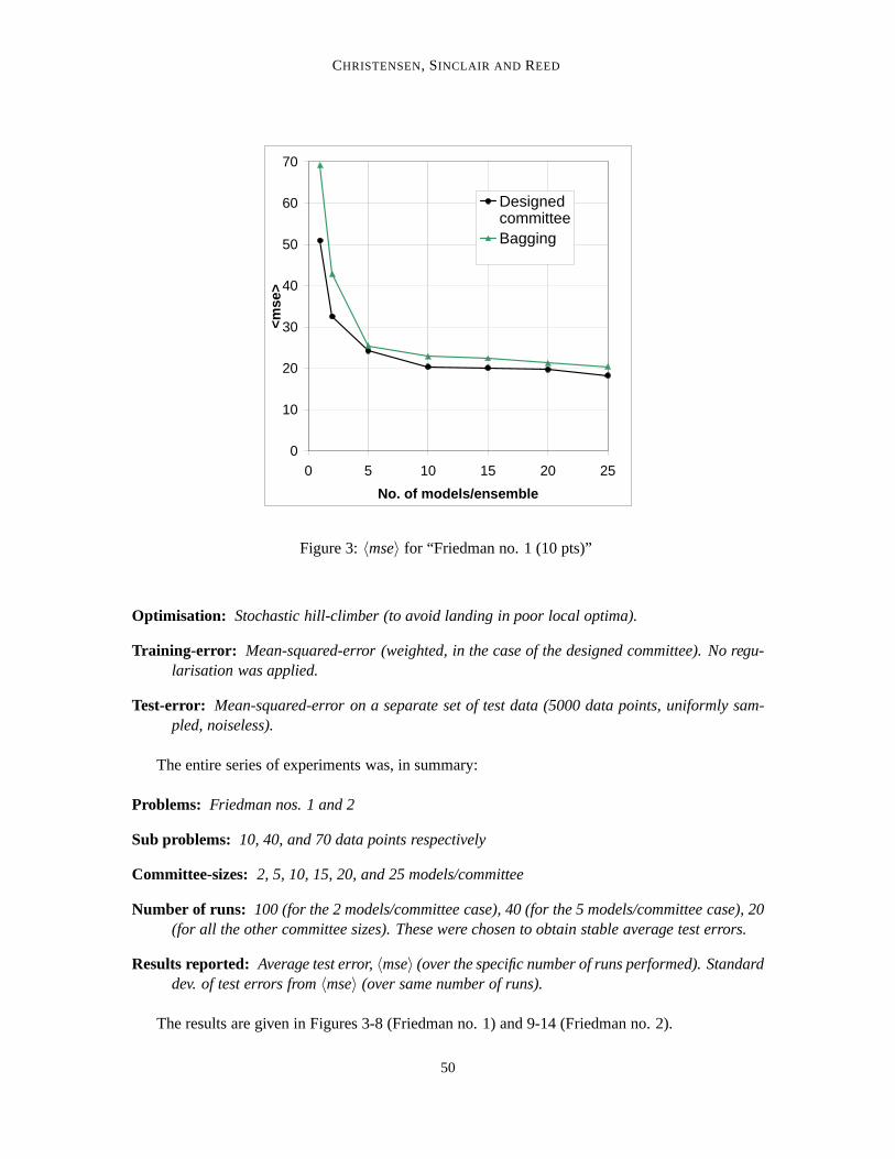
Figure 3:〈mse〉 for “Friedman no. 1 (10 pts)”
Optimisation: Stochastic hill-climber (to avoid landing in poor local optima).
Training-error: Mean-squared-error (weighted, in the case of the designed committee). No regu-larisation was applied.
Test-error: Mean-squared-error on a separate set of test data (5000 data points, uniformly sam-pled, noiseless).
The entire series of experiments was, in summary:
Problems: Friedman nos. 1 and 2
Sub problems: 10, 40, and 70 data points respectively
Committee-sizes: 2, 5, 10, 15, 20, and 25 models/committee
Number of runs: 100 (for the 2 models/committee case), 40 (for the 5 models/committee case), 20(for all the other committee sizes). These were chosen to obtain stable average test errors.
Results reported: Average test error,〈mse〉 (over the specific number of runs performed). Standarddev. of test errors from〈mse〉 (over same number of runs).
The results are given in Figures 3-8 (Friedman no. 1) and 9-14 (Friedman no. 2).
50
DESIGNING COMMITTEES OFMODELS THROUGHDELIBERATE WEIGHTING OF DATA POINTS
0
5
10
15
20
25
0 5 10 15 20 25
No. of models/ensemble
Std
.Dev
.(<m
se>)
DesignedcommitteeBagging
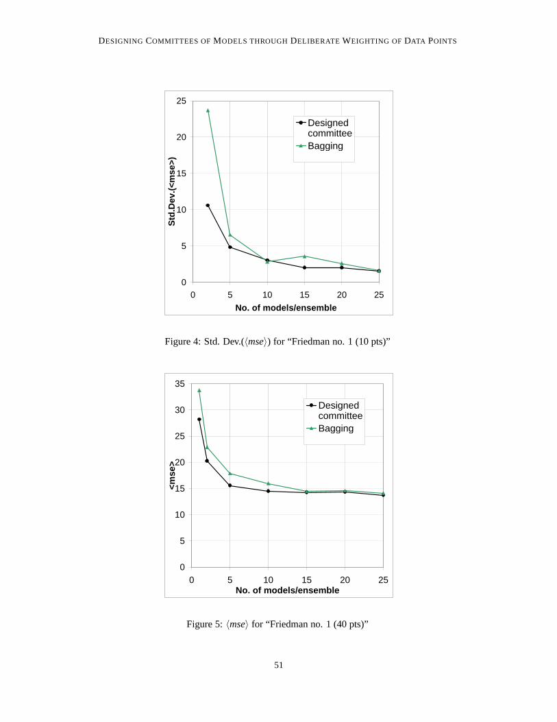
Figure 4: Std. Dev.(〈mse〉) for “Friedman no. 1 (10 pts)”
0
5
10
15
20
25
30
35
0 5 10 15 20 25No. of models/ensemble
<mse
>
DesignedcommitteeBagging
Figure 5:〈mse〉 for “Friedman no. 1 (40 pts)”
51
CHRISTENSEN, SINCLAIR AND REED
0.0
0.5
1.0
1.5
2.0
2.5
3.0
3.5
4.0
4.5
5.0
0 5 10 15 20 25No. of models/ensemble
Std
.Dev
.(<m
se>)
DesignedcommitteeBagging
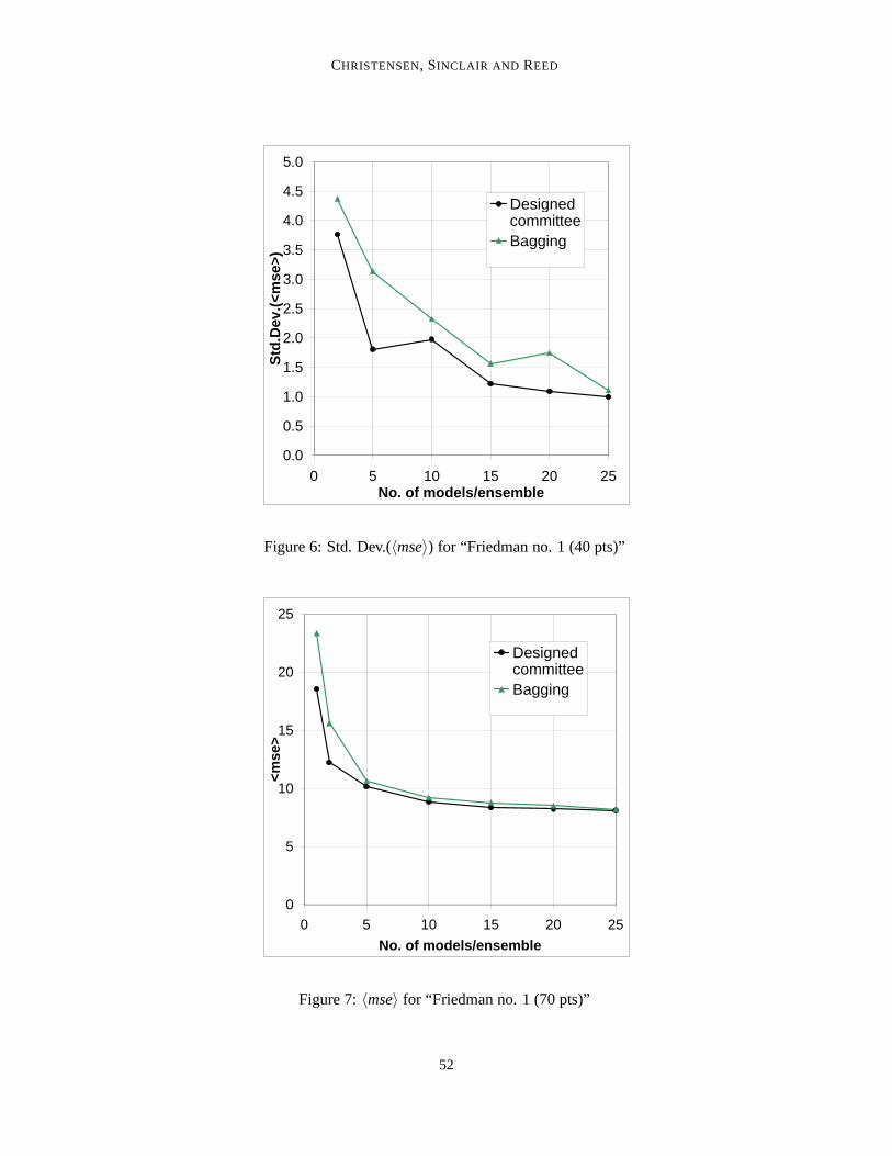
Figure 6: Std. Dev.(〈mse〉) for “Friedman no. 1 (40 pts)”
0
5
10
15
20
25
0 5 10 15 20 25
No. of models/ensemble
<mse
>
DesignedcommitteeBagging
Figure 7:〈mse〉 for “Friedman no. 1 (70 pts)”
52
DESIGNING COMMITTEES OFMODELS THROUGHDELIBERATE WEIGHTING OF DATA POINTS
0.0
0.5
1.0
1.5
2.0
2.5
3.0
3.5
4.0
4.5
5.0
0 5 10 15 20 25No. of models/ensemble
Std
.Dev
.(<m
se>)
DesignedcommitteeBagging
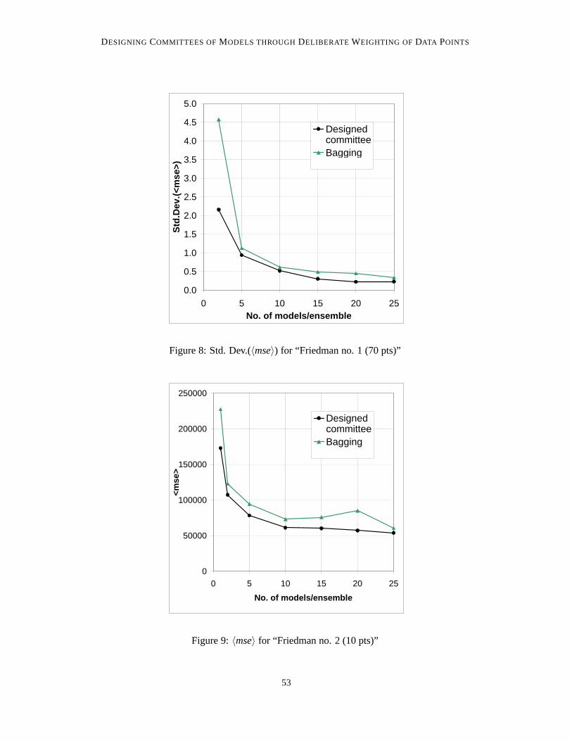
Figure 8: Std. Dev.(〈mse〉) for “Friedman no. 1 (70 pts)”
0
50000
100000
150000
200000
250000
0 5 10 15 20 25
No. of models/ensemble
<mse
>
DesignedcommitteeBagging
Figure 9:〈mse〉 for “Friedman no. 2 (10 pts)”
53
CHRISTENSEN, SINCLAIR AND REED
0
5000
10000
15000
20000
25000
30000
35000
40000
0 5 10 15 20 25
No. of models/ensemble
Std
.Dev
.(<m
se>)
DesignedcommitteeBagging
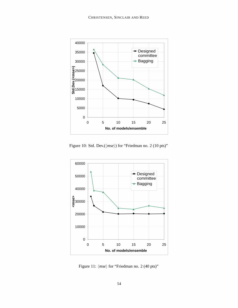
Figure 10: Std. Dev.(〈mse〉) for “Friedman no. 2 (10 pts)”
0
10000
20000
30000
40000
50000
60000
0 5 10 15 20 25
No. of models/ensemble
<mse
>
DesignedcommitteeBagging
Figure 11:〈mse〉 for “Friedman no. 2 (40 pts)”
54
DESIGNING COMMITTEES OFMODELS THROUGHDELIBERATE WEIGHTING OF DATA POINTS
0
5000
10000
15000
20000
25000
0 5 10 15 20 25
No. of models/ensemble
Std
.Dev
.(<m
se>)
DesignedcommitteeBagging
Figure 12: Std. Dev.(〈mse〉) for “Friedman no. 2 (40 pts)”
0
5000
10000
15000
20000
25000
30000
35000
40000
0 5 10 15 20 25
No. of models/ensemble
<mse
>
DesignedcommitteeBagging
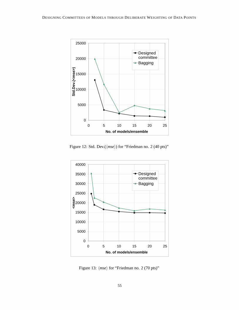
Figure 13:〈mse〉 for “Friedman no. 2 (70 pts)”
55
CHRISTENSEN, SINCLAIR AND REED
0
2000
4000
6000
8000
10000
12000
14000
16000
18000
20000
0 5 10 15 20 25
No. of models/ensemble
Std
.Dev
.(<m
se>)
DesignedcommitteeBagging
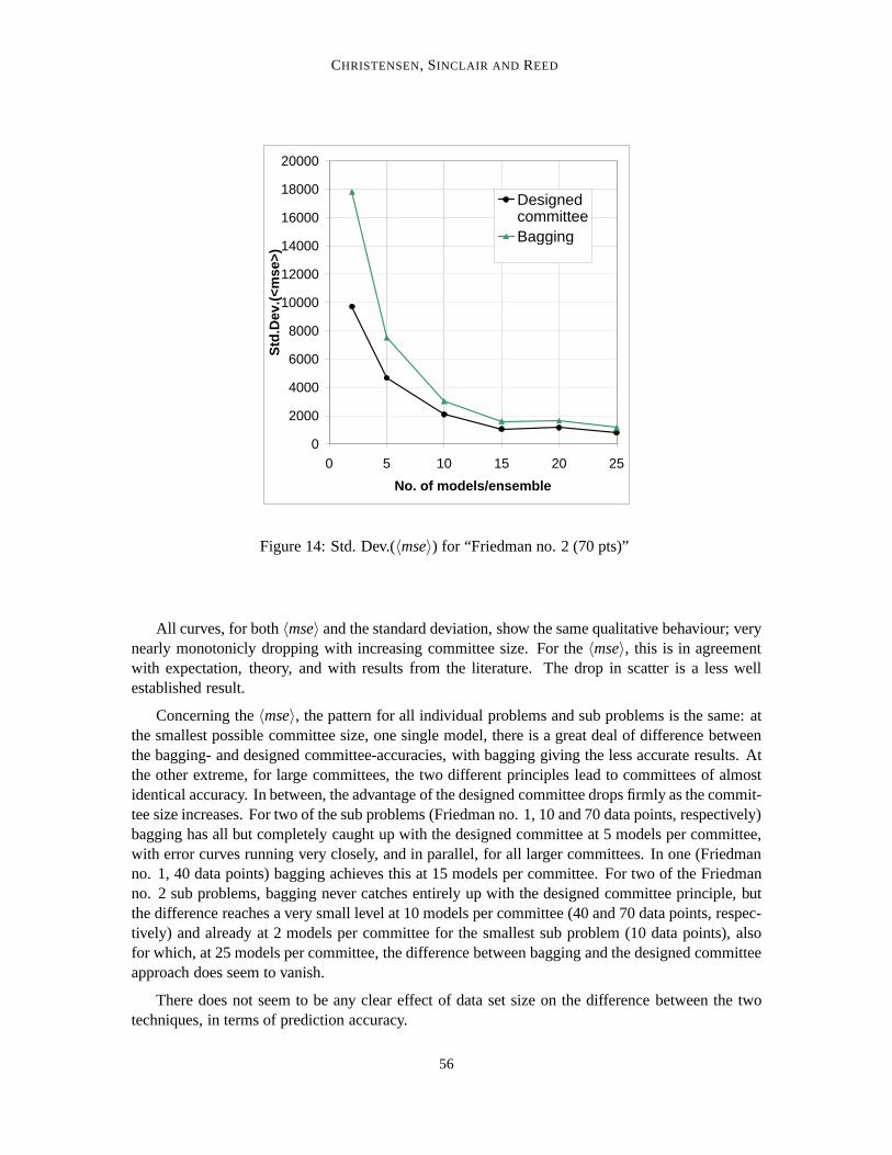
Figure 14: Std. Dev.(〈mse〉) for “Friedman no. 2 (70 pts)”
All curves, for both〈mse〉 and the standard deviation, show the same qualitative behaviour; verynearly monotonicly dropping with increasing committee size. For the〈mse〉, this is in agreementwith expectation, theory, and with results from the literature. The drop in scatter is a less wellestablished result.
Concerning the〈mse〉, the pattern for all individual problems and sub problems is the same: atthe smallest possible committee size, one single model, there is a great deal of difference betweenthe bagging- and designed committee-accuracies, with bagging giving the less accurate results. Atthe other extreme, for large committees, the two different principles lead to committees of almostidentical accuracy. In between, the advantage of the designed committee drops firmly as the commit-tee size increases. For two of the sub problems (Friedman no. 1, 10 and 70 data points, respectively)bagging has all but completely caught up with the designed committee at 5 models per committee,with error curves running very closely, and in parallel, for all larger committees. In one (Friedmanno. 1, 40 data points) bagging achieves this at 15 models per committee. For two of the Friedmanno. 2 sub problems, bagging never catches entirely up with the designed committee principle, butthe difference reaches a very small level at 10 models per committee (40 and 70 data points, respec-tively) and already at 2 models per committee for the smallest sub problem (10 data points), alsofor which, at 25 models per committee, the difference between bagging and the designed committeeapproach does seem to vanish.
There does not seem to be any clear effect of data set size on the difference between the twotechniques, in terms of prediction accuracy.
56

DESIGNING COMMITTEES OFMODELS THROUGHDELIBERATE WEIGHTING OF DATA POINTS
The monotonic character is rigorous for all curves, except bagging in Friedman no. 2 (notablynon-monotonic for the 40 data points sub problem).
The monotonicity is broken rather more severely for the scatter curves; for bagging this appliesto both the 40 data points sub problems and one of the 10 data point ones (Friedman no. 1). It alsoapplies to the designed committee on Friedman no. 1 (40 data points).
A general pattern, concerning the difference between bagging and the designed committee interms of the scatter, is more difficult to identify. For both the 70 data point sub problems, thedesigned committees’ have much less scatter at 2 models/committee, but bagging quickly catchesup. The same seems to be the case for Friedman no. 1 (10 data points). For Friedman no. 1 (40 datapoints), however, no trend is obvious; for Friedman no. 2 (40 data points), bagging is only reallyclose to the designed approach at 10 models/committee, with the latter method having much lowerscatter for all other committee sizes. Finally, for Friedman no. 2 (10 data points), the two methodsseems to have nearly the same scatter at 2 models/committee, with bagging having much higherscatter for all other committee sizes.
Overall it can be said that the designed approach never obtained an〈mse〉 larger than the cor-responding bagging committee, and only in one case (Friedman no. 1, 10 data points, 10 mod-els/committee) did it have larger scatter (and only marginally so).
4.2 Ozone data set
The Ozone data set has, like the Miles per Gallon set in Section 4.3, been obtained from the UCIRepository Of Machine Learning Databases and Domain Theories (Murphy and Aha, 1994) but itis originally from (Breiman and Friedman, 1985). It contains 13 variables and 366 data points but,owing to missing data in the set, the number of inputs has been reduced to 8 (with one output) and330 data points. It is a real life data set, concerning climate measurements.
The modelling undertaken here was as follows:
Architecture: MLP with 3 hidden layer neurons (a single hidden layer), andtanhactivation func-tion.
Optimisation: Downhill simplex with multiple restart (15 runs, best model retained).
Training-error: Mean-squared-error (weighted, in the case of the designed committee). No regu-larisation was applied.
Test-error: Cross-validation, with 80% data for training and 20% for testing.
The entire series of experiments was, in summary:
Committee-sizes: 1, 2, 5, 10, 20, and 40 models/committee
Number of runs: 200 (for the 1 model/committee case), 100 (for the 2 models/committee case),40 (5 models/committee), 20 (10 models/committee), 10 (20 models/committee) and 5 (40models/committee). These were chosen to obtain stable average test errors.
Results reported: Average test error,〈mse〉 (over the specific number of runs performed). Standarddev. of test errors from〈mse〉 (over same number of runs).
57
CHRISTENSEN, SINCLAIR AND REED
0
5
10
15
20
25
30
35
40
0 5 10 15 20 25 30 35 40
No. of models/ensemble
<mse
>
DesignedcommitteeBagging
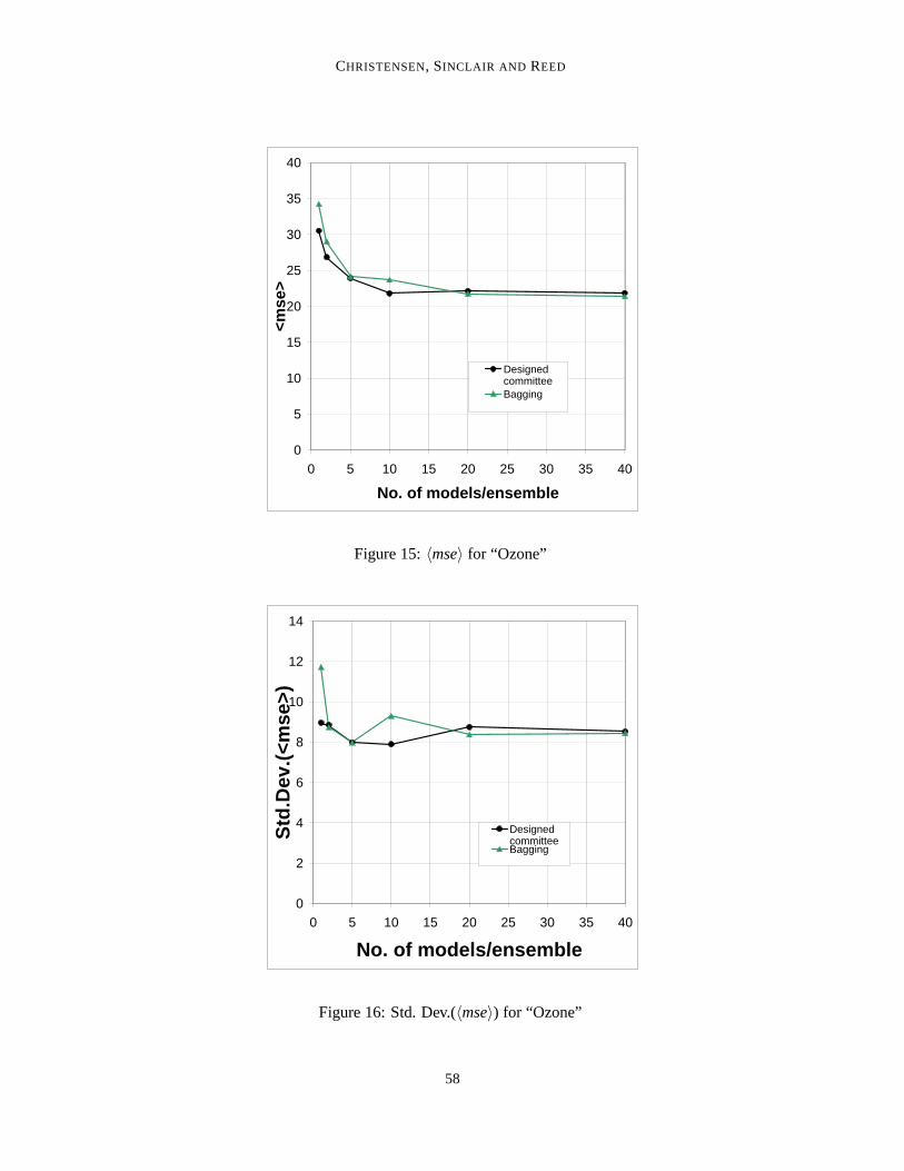
Figure 15:〈mse〉 for “Ozone”
0
2
4
6
8
10
12
14
0 5 10 15 20 25 30 35 40
No. of models/ensemble
Std
.Dev
.(<m
se>)
DesignedcommitteeBagging
Figure 16: Std. Dev.(〈mse〉) for “Ozone”
58

DESIGNING COMMITTEES OFMODELS THROUGHDELIBERATE WEIGHTING OF DATA POINTS
Results appear in Figures 15-16.The 〈mse〉 pattern is slightly different from in the Friedman examples. Though the designed
committee approach outperforms bagging considerably at committee sizes of 1, 2 and 10 models,bagging actually performs best at 20 and 40 models per committee, albeit only by very little margin.The overall picture is consistent with the Friedman examples: small committees⇒ bagging isinferior; large committees⇒ bagging is at least as good as the designed approach (and here actuallybetter).
For bagging, the scatter in〈mse〉 again seems to drop with committee size, but no clear trendappears for the designed committee approach.
4.3 Miles per Gallon data set
The Miles per Gallon data set, in the present version obtained from the UCI Repository, originatedin the StatLib library, which is maintained at Carnegie Mellon University. It contains 9 variablesand 398 data points but, owing to missing data in the set, the number of inputs has been reduced to7 (with one output) and 392 data points. It is a real life data set, concerning fuel economy in cars.
The modelling undertaken here was as follows:
Architecture: MLP with 3 hidden layer neurons (a single hidden layer), andtanhactivation func-tion.
Optimisation: Downhill simplex with multiple restart (15 runs, best model retained).
Training-error: Mean-squared-error (weighted, in the case of the designed committee). No regu-larisation was applied.
Test-error: Cross-validation, with 75% data for training and 25% for testing.
The entire series of experiments was, in summary:
Committee-sizes: 1, 2, 5, 10, 20, and 40 models/committee
Number of runs: 160 (for the 1 model/committee case), 80 (2 models/committee), 32 (5 mod-els/committee), 16 (10 models/committee), 8 (20 models/committee) and 4 (40 models/committee).These were chosen to obtain stable average test errors.
Results reported: Average test error,〈mse〉 (over the specific number of runs performed). Standarddev. of test errors from〈mse〉 (over same number of runs).
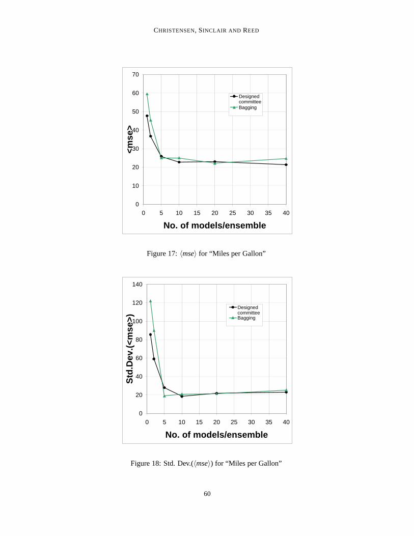
Results appear in Figures 17-18.Again at small committees the designed approach fares better in terms of〈mse〉, but from 5
models and upwards the two techniques are rather equal though at the very largest committee size(40 models) bagging performs considerably worse than at the 20 model/com-mittee size, as wellas worse than the designed approach. The drop in〈mse〉 with committee size is not consistent forbagging; it is for the designed committee approach however.
〈Mse〉 scatter drops rapidly for both methods, with bagging having significantly less at 5 mod-els/committee than the designed approach. For smaller committees it is the other way around; forlarger ones the two methods attain almost identical levels.
59
CHRISTENSEN, SINCLAIR AND REED
0
10
20
30
40
50
60
70
0 5 10 15 20 25 30 35 40
No. of models/ensemble
<mse
>
DesignedcommitteeBagging
Figure 17:〈mse〉 for “Miles per Gallon”
0
20
40
60
80
100
120
140
0 5 10 15 20 25 30 35 40
No. of models/ensemble
Std
.Dev
.(<m
se>)
DesignedcommitteeBagging
Figure 18: Std. Dev.(〈mse〉) for “Miles per Gallon”
60

DESIGNING COMMITTEES OFMODELS THROUGHDELIBERATE WEIGHTING OF DATA POINTS
4.4 Schwefel 3.2 data set
The Schwefel 3.2 data set comes from a function given by Schwefel (1981) and it is less wellknown in the modelling community. It is an artificial problem, the data arising from sampling of thefunction:
f (x) =3
∑i=2
[(x1−x2i )
2 + (1−xi)2]
For the present use, 100 data points were sampled, input values randomly distributed over theinterval [-5,5] for all inputs. To the data sampled was not added any noise.
The modelling undertaken was as follows:
Architecture: MLP with 7 hidden layer neurons (a single hidden layer), andtanhactivation func-tion.
Optimisation: Downhill simplex with multiple restart (15 runs, best model retained).
Training-error: Mean-squared-error (weighted, in the case of the designed committee). No regu-larisation was applied.
Test-error: Cross-validation, with 75% data for training and 25% for testing.
The entire series of experiments was, in summary:
Committee-sizes: 1, 2, 5, 10, 20, and 40 models/committee
Number of runs: 160 (for the 1 model/committee case), 80 (2 models/committee), 32 (5 mod-els/committee), 16 (10 models/committee), 8 (20 models/committee) and 4 (40 models/committee).These were chosen to obtain stable average test errors.
Results reported: Average test error,〈mse〉 (over the specific number of runs performed). Standarddev. of test errors from〈mse〉 (over same number of runs).
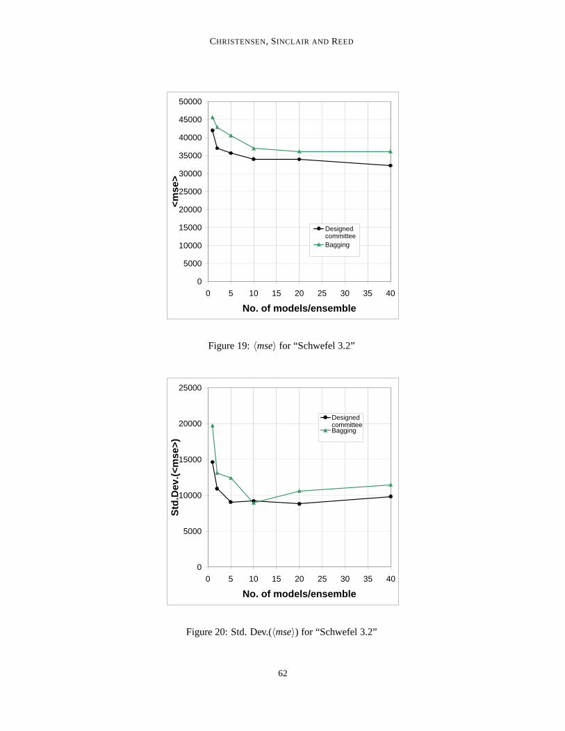
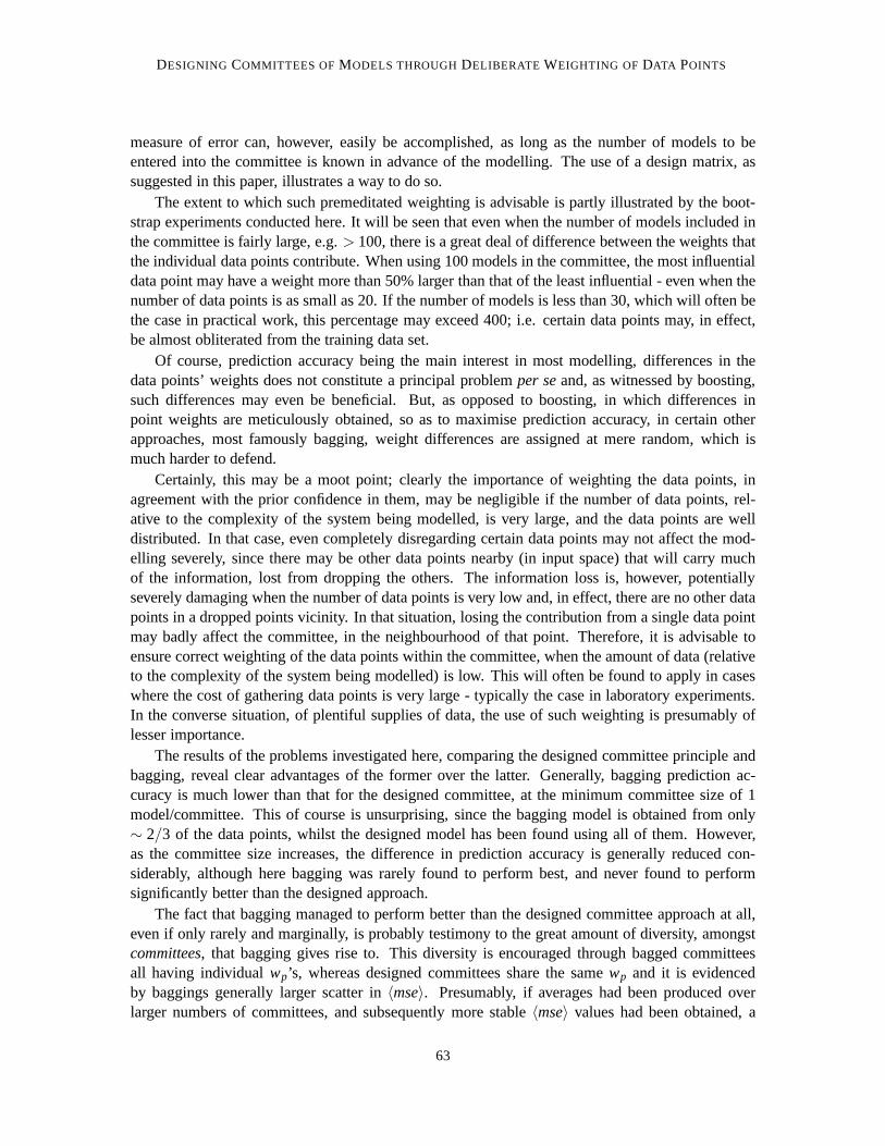
Results appear in Figures 19-20.In this experiment, bagging is outdone rather extensively, in terms of〈mse〉, at all committee
sizes; even at 40 models/committee has bagging failed to catch up. Also in terms of〈mse〉 scatterhas the designed committee approach got significantly lower values, except at 10 models/committee,where the two methods attain roughly the same level.
5. Discussion
The usefulness of weighting models individually in committee based modelling, and of taking theconfidence in the individual data points into consideration when deriving models, has been under-stood for decades; however these principles are not usually employed in conjunction. Deliberateweighting of data points is normally not a concern in the construction of committees, and very un-equal weights may be given to data points of the same provenance; a fact that will generally meetwith little understanding from the data owners, who have gathered the data.
Weighting the contribution of the individual data points, to the error-measure employed in thetraining phase, so that every data point contributes with a pre-specified weight to thecommittees
61
CHRISTENSEN, SINCLAIR AND REED
0
5000
10000
15000
20000
25000
30000
35000
40000
45000
50000
0 5 10 15 20 25 30 35 40
No. of models/ensemble
<mse
>
DesignedcommitteeBagging
Figure 19:〈mse〉 for “Schwefel 3.2”
0
5000
10000
15000
20000
25000
0 5 10 15 20 25 30 35 40
No. of models/ensemble
Std
.Dev
.(<m
se>)
DesignedcommitteeBagging
Figure 20: Std. Dev.(〈mse〉) for “Schwefel 3.2”
62
DESIGNING COMMITTEES OFMODELS THROUGHDELIBERATE WEIGHTING OF DATA POINTS
measure of error can, however, easily be accomplished, as long as the number of models to beentered into the committee is known in advance of the modelling. The use of a design matrix, assuggested in this paper, illustrates a way to do so.
The extent to which such premeditated weighting is advisable is partly illustrated by the boot-strap experiments conducted here. It will be seen that even when the number of models included inthe committee is fairly large, e.g.> 100, there is a great deal of difference between the weights thatthe individual data points contribute. When using 100 models in the committee, the most influentialdata point may have a weight more than 50% larger than that of the least influential - even when thenumber of data points is as small as 20. If the number of models is less than 30, which will often bethe case in practical work, this percentage may exceed 400; i.e. certain data points may, in effect,be almost obliterated from the training data set.
Of course, prediction accuracy being the main interest in most modelling, differences in thedata points’ weights does not constitute a principal problemper seand, as witnessed by boosting,such differences may even be beneficial. But, as opposed to boosting, in which differences inpoint weights are meticulously obtained, so as to maximise prediction accuracy, in certain otherapproaches, most famously bagging, weight differences are assigned at mere random, which ismuch harder to defend.
Certainly, this may be a moot point; clearly the importance of weighting the data points, inagreement with the prior confidence in them, may be negligible if the number of data points, rel-ative to the complexity of the system being modelled, is very large, and the data points are welldistributed. In that case, even completely disregarding certain data points may not affect the mod-elling severely, since there may be other data points nearby (in input space) that will carry muchof the information, lost from dropping the others. The information loss is, however, potentiallyseverely damaging when the number of data points is very low and, in effect, there are no other datapoints in a dropped points vicinity. In that situation, losing the contribution from a single data pointmay badly affect the committee, in the neighbourhood of that point. Therefore, it is advisable toensure correct weighting of the data points within the committee, when the amount of data (relativeto the complexity of the system being modelled) is low. This will often be found to apply in caseswhere the cost of gathering data points is very large - typically the case in laboratory experiments.In the converse situation, of plentiful supplies of data, the use of such weighting is presumably oflesser importance.
The results of the problems investigated here, comparing the designed committee principle andbagging, reveal clear advantages of the former over the latter. Generally, bagging prediction ac-curacy is much lower than that for the designed committee, at the minimum committee size of 1model/committee. This of course is unsurprising, since the bagging model is obtained from only∼ 2/3 of the data points, whilst the designed model has been found using all of them. However,as the committee size increases, the difference in prediction accuracy is generally reduced con-siderably, although here bagging was rarely found to perform best, and never found to performsignificantly better than the designed approach.
The fact that bagging managed to perform better than the designed committee approach at all,even if only rarely and marginally, is probably testimony to the great amount of diversity, amongstcommittees, that bagging gives rise to. This diversity is encouraged through bagged committeesall having individualwp’s, whereas designed committees share the samewp and it is evidencedby baggings generally larger scatter in〈mse〉. Presumably, if averages had been produced overlarger numbers of committees, and subsequently more stable〈mse〉 values had been obtained, a
63
CHRISTENSEN, SINCLAIR AND REED
completely consistent pattern would have emerged. This is of course speculation at present, andonly larger scale experiments will reveal whether this assumption holds or not.
A very consistent picture emerged of〈mse〉 scatter dropping with increasing committee sizeuntil levelling off at large committee sizes. What causes this effect, which applies to both methods,is not clear; conceivably it is an artefact reflecting the general modelling schedule used for bothtechniques. For all experiments in this study, the number of committees over which the averageswere obtained dropped with increasing committee size; when large, the committees are likely to bequite similar, leading to similar〈mse〉s; when small, the committees are likely to be quite dissimilar,leading to dissimilar〈mse〉s. For now, this is our preferred explanation of the effect.
In the Friedman problems, no clear effect could be found, of overall data point density, on theperformance difference between the proposed approach and bagging; this runs somewhat counterto expectation but can possibly be explained as a result of the data point density being very low forall the data sets, even the largest. Further experimental work will be required to elucidate this issueproperly.
A real concern with the proposed framework, may be that the process outlined is designed; i.e.how many models, and data points, are to be included must be known in advance of the modelling,;this may, or may not, be practical for the modelling task at hand. As shown, this does not preventthe possibility of enlarging an already existing committee; in other words, should a given committeebe considered inadequate, it can be augmented by further models at any point, and these may evenbe obtained on different data from those used originally.
The core concept in the proposed framework is the design matrix; this is bestowed with a greatdeal of freedom, allowing the information contained in the data to be distributed over the individualmodels according to a great many principles. “Random” distribution has been shown, as has distri-bution following a cross-validation scheme. Other principles could be employed as well, wherebythe distribution is based on certain properties of the data points. Inherent to these are their locationsin input/output space, and from this a distribution not unlike that of mixtures-of-experts can be ob-tained. Typically, however, there may be more pieces of information stored with the data than thoseeventually employed in the modelling. Such additional properties may also form the basis of thedistribution of information across the committee’s models.
An intrinsic obstacle lies herein, in the sense that obtaining an appropriate design matrix mayitself require a modelling exercise, though possibly a less complicated one, prior to the actual mod-elling of the targeted system. The obvious advantage of course, is that tailor-made distributions canindeed be obtained. It must be remembered, however, that the driving force behind the distributionof information across models should at all times be the attempt to maximise the differences betweenthese models, as this is the prime means through which a committee exercises its superiority over asingle model, with respect to system approximation.
6. Conclusions
In this paper, a new, systematic approach to the formation of committees, by way of a design matrix,has been introduced. Each data point contributes with a prespecified, overall weight to the trainingof the committee, whilst contributing with unequal specific weights in the training of the constituentmodels, thus encouraging model diversity. The overall weight should be assigned based on the priorconfidence in the data point; if all are considered equally reliable, each should be given the sameoverall weight.
64
DESIGNING COMMITTEES OFMODELS THROUGHDELIBERATE WEIGHTING OF DATA POINTS
Within this framework, different principles may be used to distribute the influence of the indi-vidual data points over the committee’s models. Thus bagging is a special case, corresponding to aparticular type of distribution; the binary distribution inherent to cross-validation may be used, andmixtures-of-experts may be emulated though, owing to the strictly adaptive nature of that approach,it cannot be fully implemented. This same discordance, between adaptive and designed modelling,prevents boosting from being directly implementable under the proposed framework.
In the paper it has been shown how to augment an existing committee by additional models,whether these be built on the original data, or on all/partly new data, such that the resulting commit-tee places the desired emphasis on each data point.
Further, use of the design matrix has been conjectured, on theoretical grounds, to be particularlyadvisable when the number of data points available, relative to the complexity of the system tobe modelled, is low; if the supply of data points is relatively generous, however, it may be a nearredundant exercise. Counter to the theoretical argument, the actual experiments carried out here didnot show this, possibly because all sub problems studied had very few data points.
Finally, in a direct head-to-head comparison with bagging, the theoretical advantage of thedesigned committee, due to its “fairer” weighting of the information contained in the data, wouldseem to be supported by the numerical experiments carried out here. It must be acknowledgedthat the number and variety of these experiments is insufficient to warrant very strong conclusions,but, on the other hand, the clear pattern that emerged, and the agreement between this and theory,constitutes a strong argument for the case of premeditated weighting of data points during committeetraining.
Acknowledgments
SWC thanks Dr. Steve Gunn for numerous stimulating discussions in the general area of machinelearning.
References
L. Breiman. Bagging predictors. Machine Learning 24 (2):123-140,1996.
L. Breiman. Randomizing outputs to increase prediction accuracy. Technical Report No. 518. De-partment of Statistics, UC Berkeley, 1998.
L. Breiman. Combining predictors. In Amanda J. C. Sharkey, editor, Combining Artificial Neu-ral Nets. Ensemble and Modular Multi-Net Systems, Perspectives in Neural Computing, 31-50.Springer, 1999.
L. Breiman & J. H. Friedman. Estimating optimal transformations for multiple regression and cor-relation. Journal of the American Statistical Association, 80, 580-619, 1985.
T. G. Dietterich. Ensemble methods in machine learning. In J. Kittler and F. Roli, editors, MultipleClassier Systems, vol. 1857 of Lecture Notes in Computer Science, pages 1-15, Cagliari, Italy,Springer, 2000.
J. H. Friedman. Multivariate adaptive regression splines. The Annals of Statistics, 19 (1), 1-141,1991.
65
CHRISTENSEN, SINCLAIR AND REED
L. K. Hansen, & P. Salamon. Neural network ensembles. IEEE Transactions on Pattern Analysisand Machine Intelligence, vol. 12. No. 10, 993-1000, 1990.
S. Hashem. Optimal linear combinations of neural networks. Neural Networks, vol. 10 (4), 599-614,1997.
R. A. Jacobs, M. I. Jordan, S. J. Nowlan, and G. E. Hinton. Adaptive mixtures of local experts.Neural Computation 3, 79-87, 1991.
A. Krogh, & J. Vedelsby. Neural network ensembles, cross validation, and active learning. In G.Tesauro, D. S. Touretzky and T. K. Leen, eds. Advances in neural information processing systems7, 231-238, MIT Press, Cambridge MA, 1995.
Y. Liao, & J. Moody. Constructing Heterogeneous Committees Using Input Feature Grouping: Ap-plication to Economic Forecasting. In Advances in Neural Information Processing Systems 12,S. A. Solla, T. K. Leen, K.-R. Mller, eds., MIT Press, 2000.
Y. Liu. & X. Yao. A Cooperative Ensemble Learning System. In Proc. of the 1998 IEEE Interna-tional Joint Conference on Neural Networks (IJCNN’98), pp.2202-2207, Anchorage, USA, 1998.
Y. Liu, & X. Yao. Ensemble learning via negative correlation. Neural Networks 12, 1399-1404,1999.
C. J. Mertz. Classification and regression by combining models. Ph.D. thesis, UC Irvine, 1998.
P. M. Murphy & D. W. Aha. UCI Repository of machine learning databases. University of Califor-nia, Department of Information and Computer Science. Irvine, CA (1994).
D. W. Opitz, & J. W. Shavlik. Actively searching for an effective neural-network ensemble. Con-nection Sci., 8 (3-4), 1996.
M. P. Perrone, & L. N. Cooper. When networks disagree: Ensemble methods for hybrid neuralnetworks. In R. J. Mammone, editor, Neural Networks for Speech and Image Processing, 1993.
Y. Raviv, & N. Intrator. Bootstrapping with noise: An effective regularization technique. ConnectionScience, Special issue on combining estimators, 8:356-372, 1996.
B. E. Rosen. Ensemble Learning using Decorrelated Neural Networks. Connection Science, Vol. 8,No. 3-4, pp. 373-384, 1996.
H. Schwefel. Numerical Optimization of Computer Models. Wiley, New York, 1981.
R. Shapire. The strength of weak learnability. Machine Learning, 5 (2), 197-227, 1990.
66