Embed Size (px)
Citation preview

HAL Id: tel-01532315https://tel.archives-ouvertes.fr/tel-01532315
Submitted on 2 Jun 2017
HAL is a multi-disciplinary open accessarchive for the deposit and dissemination of sci-entific research documents, whether they are pub-lished or not. The documents may come fromteaching and research institutions in France orabroad, or from public or private research centers.
L’archive ouverte pluridisciplinaire HAL, estdestinée au dépôt et à la diffusion de documentsscientifiques de niveau recherche, publiés ou non,émanant des établissements d’enseignement et derecherche français ou étrangers, des laboratoirespublics ou privés.
Development of dispersion tailored optical fibers forultrafast 2 µm lasers
Mathieu Jossent
To cite this version:Mathieu Jossent. Development of dispersion tailored optical fibers for ultrafast 2 µm lasers. Optics /Photonic. Université de Limoges, 2017. English. �NNT : 2017LIMO0016�. �tel-01532315�

Université de Limoges
École Doctorale Sciences et Ingénierie pour l’Information, Mathématiques (ED 521)
XLIM CNRS UMR-7252 Axe Photonique
Thèse pour obtenir le grade de
Docteur de l’Université de Limoges Mention : Électronique des Hautes Fréquences, Photonique et Systèmes
Présentée et soutenue par
Mathieu Jossent
Le 4 mai 2017
Thèse dirigée par Sébastien Février
JURY :
Président du jury M. Philippe DI BIN Professeur
XLIM, Université de Limoges
Rapporteurs
M. Jayanta SAHU Professeur ORC, Université de Southampton
M. Ammar HIDEUR Maître de conférences HDR CORIA, Université de Rouen
Examinateur M. Laurent BIGOT Chargé de recherche 1 CNRS – HDR
PhLAM, Université de Lille 1
Invités M. Arnaud GRISARD Ingénieur
TRT, Thales, Palaiseau
M. Sébastien FEVRIER Maître de conférences HDR XLIM, Université de Limoges
Développement de fibres optiques à dispersion contrôlée pour l’élaboration de lasers ultrarapides à 2 µm.
Development of dispersion tailored optical fibers for ultrafast 2 µm lasers
Thèse de doctorat


Mathieu Jossent | Thèse de doctorat | Université de Limoges | 2017 iii
To my family

Mathieu Jossent | Thèse de doctorat | Université de Limoges | 2017 iv
Copyright
Cette création est mise à disposition selon le Contrat :
« Attribution-Pas d'Utilisation Commerciale-Pas de modification 3.0 France »
disponible en ligne : http://creativecommons.org/licenses/by-nc-nd/3.0/fr/

Mathieu Jossent | Thèse de doctorat | Université de Limoges | 2017 v
Table of contents
Chapter I. Context ................................................................................................................. 1
I.1. Nonlinearities in optical fibers ....................................................................................... 1
I.1.1. Optical Kerr effect .................................................................................................. 2
I.1.2. Stimulated Raman scattering ................................................................................. 5
I.1.3. Nonlinear Schrödinger equation ............................................................................ 6
I.2. Generalized nonlinear Schrödinger equation ............................................................... 9
I.2.1. Modeling the propagation of short pulses in optical fibers ...................................... 9
I.2.2. Pulse in the anomalous dispersion regime: Solitons .............................................11
I.2.2.1. Soliton theory .................................................................................................11
I.2.2.2. Soliton laser ...................................................................................................12
I.2.3. Pulse in the normal dispersion regime: Similaritons ..............................................12
I.2.3.1. Similariton theory ...........................................................................................12
I.2.3.2. Similariton laser .............................................................................................14
I.3. Ultrafast high power amplifiers ....................................................................................15
I.3.1. High energy chirped pulse amplifier ......................................................................15
I.3.2. High energy parabolic amplifier ............................................................................18
I.4. Conclusion ..................................................................................................................19
Chapter II. Modeling of a dispersion tailored few mode fiber.................................................21
II.1. Principle of operation .................................................................................................23
II.2. Design criteria ............................................................................................................24
II.3. Improved design ........................................................................................................25
II.4. Modeling towards optimal design ...............................................................................26
II.4.1. Impact of the ring .................................................................................................29
II.4.2. Impact of the trench .............................................................................................30
II.5. Fabricated passive few-mode fiber.............................................................................32
II.6. Conclusion .................................................................................................................33
Chapter III. Mode conversion in optical fibers .......................................................................34
III.1. Long period gratings with controlled bandwidth .........................................................34
III.2. Modeling and realization of a dedicated mode converter ...........................................40
III.3. Passive few mode fiber excited by the LP02 mode converter .....................................45
III.3.1. S² measurement on the passive few mode fiber excited by the mode converter .47
III.3.1.1. Erbium bandwidth ........................................................................................47
III.3.1.2. Thulium bandwidth .......................................................................................48
III.4. SFSS from 1.6 to 2 um: pulsed seed source for similariton amplifier .........................49
III.5. Dispersion measurement ..........................................................................................51
III.6. Conclusion ................................................................................................................53
Chapter IV. Few-mode Thulium-doped fiber towards a parabolic amplifier ...........................54
IV.1. Singlemode TDFA ....................................................................................................54
IV.2. Numerical procedure ................................................................................................56
IV.2.1. Multimode amplification in continuous wave regime ...........................................58
IV.2.1.1. Dependence of the gain on the pump wavelength .......................................58
IV.2.1.2. Spatial evolution of the LP02 weight along amplification ...............................60
IV.2.1.3. Enhanced design .........................................................................................62
IV.2.2. Nonlinear modeling ............................................................................................64
IV.2.2.1. Constant effective modal area and gain .......................................................65

Mathieu Jossent | Thèse de doctorat | Université de Limoges | 2017 vi
IV.2.2.1.1. Unrealistic 1 ps pulse ............................................................................65
IV.2.2.1.2. Realistic 100 fs pulse ............................................................................68
IV.2.2.2. Effective modal area ....................................................................................71
IV.2.2.2.1. Unrealistic 1 ps pulse ............................................................................71
IV.2.2.2.2. Realistic 100 fs pulse ............................................................................72
IV.2.2.3. Gain .............................................................................................................74
IV.2.2.4. Effective area and gain ................................................................................75
IV.3. Fabricated active few-mode fiber ..............................................................................77
IV.4. Conclusion ................................................................................................................79
General Conclusion and prospects .......................................................................................81
Appendix. Experimental determination of the modal content by means of S2 imaging..........84
References ...........................................................................................................................95

Mathieu Jossent | Thèse de doctorat | Université de Limoges | 2017 1
Chapter I. Context
The ANR-funded project UBRIS2 aims at developing innovative ways towards the realization
of high-power ultrafast laser systems at the wavelength of 2 µm. One approach to build high-
energy lasers at 2 µm relies on parabolic amplification, a concept that has never been
explored at 2 µm so far. The 2-µm parabolic amplifier would rely on Thulium-doped fibers
with tailored high normal dispersion (high –D), providing temporal broadening along the
amplifier leading to an increase of the storable energy compared to conventional systems.
This concept has been successfully used at 1 µm where silica exhibits normal dispersion but
remains unexploited at 2 µm due to the lack of properly designed fibers. The goal of my
PhD was to design and develop parabolic amplifiers based on specialty active fibers
producing high normal dispersion at 2 µm.
Parabolic amplification or direct amplification in normal dispersion regime, yields a
particular class of pulses, the similariton, characterized by parabolic temporal and spectral
shapes that homothetically grow along the active fiber. Similaritons result from the interplay
between gain and nonlinear Kerr effect in normally dispersive materials.
In this context, this chapter gives an overview of the physical mechanisms at stake in
the formation of similaritons in optical fibers with a particular emphasis on (i) energy scaling
and (ii) transposition of this concept towards the mid-infrared. The effects of optical
nonlinearities in optical fibers are briefly reviewed. This review is followed by a description of
the generalized nonlinear Schrödinger equation with gain. Finally, state-of-the-art ultrafast
high power amplifiers based on active fibers emitting at 1 µm and 2 µm are presented with an
emphasis on the fiber design.
I.1. Nonlinearities in optical fibers
The main constituent of optical fiber is silica (SiO2). Silica is a dielectric, meaning that
the charge carriers in this material are strongly bound to one another. Hence, they are
unable to move, in a macroscopic scale, under the influence of an electrical field. However,
in a microscopic scale, the links between the charge carriers have a certain elasticity
allowing them a transitory displacement under the influence of an electrical field. Those
charge movements imply the creation of several induced dipoles within the material. The
interactions between those charge carriers and the applied electrical field generates a
polarization of the media.
In the case of a weak electromagnetic field, the polarization Pol of the material is
proportional to the applied electrical field EF by the dielectric constant 0 and the material
electrical susceptibility (1):

Mathieu Jossent | Thèse de doctorat | Université de Limoges | 2017 2
F
10ol EP (I.1)
The linear susceptibility (1) is a complex number and can therefore be expressed by its real
and imaginary parts 1''1'1 i . This parameter depends on the wavelength of the
excitation electromagnetic wave. It gives access to two parameters: the refractive index n0 of
the media and its absorption :
1'0
2
11n (I.2)
1''
0n
2 (I.3)
However, with an increased intensity of the electromagnetic field, nonlinear response of the
material could be observed. The relation (I.1) will therefore be incomplete since the material
will produce a nonlinear response to the excitation field. The polarization is therefore
expressed by:
...EEEP3
F32
F2
F1
0ol (I.4)
In this expression, the linear susceptibility (1) can be identified. The other components (j)
represent the nonlinear susceptibilities of the jth order and are responsible for nonlinear
effects within the material. In general, those effects are categorized by the order j of the
considered susceptibility.
In dielectrics composed by centro-symmetrical molecules, such as silica, (2) is
evanescent and therefore will not have any effect in optical fibers. However, this order of
susceptibility is responsible of effects such as the second harmonic generation in crystals. In
the following, the contribution of (2) will be taken equal to zero. In that way, when
considering silica based optical fibers, the nonlinear effects arise from the third order
nonlinear susceptibility (3). Some of those effects will be discussed in the following.
I.1.1. Optical Kerr effect
When an electromagnetic field of high intensity passes through a dielectric material,
the wave oscillating electrical field generates the induced electrical dipoles. The electrical
dipoles presenting the highest dipolar moment might then orientate themselves in the
electrical field direction creating local birefringence in the media. The refractive index profile
is no more a constant at a given wavelength but becomes dependent on the applied
electrical field intensity. This nonlinear index has the following expression:

Mathieu Jossent | Thèse de doctorat | Université de Limoges | 2017 3
2F20
2F t,zEnnt,zE,n (I.5)
with n0() the linear refractive index as defined previously and
0
3
2n8
3n the index
change due to the third order nonlinearity. For pure silica, 1220
2 W.m1024.2n at
1.55 µm [1]. However, this experimental value of the nonlinear index also depends on
impurities and/or dopants (Germanium, Phosphorus, Fluorine, Aluminum, rare earth ions…)
within the glass matrix.
The dependency of the refractive index to the electrical field intensity is called “optical Kerr
effect”. The wave passing through the material will locally change the refractive index of the
material in which the wave propagates. This self-process leads to an addition of a phase
term called to the wave itself. This effect is referred to as ‘self-phase modulation’ (SPM). The
phase therefore writes:
Lkt,zEnnt,z 02
F2 (I.6)
where k0 is the wave vector norm and is equal to 2/, L is the fiber length. The nonlinear
phase is 2
F02NL ELkn .
The nonlinear coefficient expresses the strength of the third order nonlinearities
arising from Kerr effect in an optical fiber and is given by [1]:
2
eff
2 n
A
(I.7)
where Aeff is the effective mode area of the fiber fundamental mode. This area represents the
zone over which the optical power is distributed and therefore depends on the transverse
repartition of the modal field.
dSE
dSE
A4
F
22
F
eff
(I.8)
with dS a surface element of the considered fiber section.
A characteristic length can also be defined and is called the nonlinear length LNL. This
parameter gives an idea of the fiber length from which nonlinear effects due to Kerr effect
become important:

Mathieu Jossent | Thèse de doctorat | Université de Limoges | 2017 4
0NL
P
1L
(I.9)
This nonlinear length depends on the nonlinear coefficient of the optical fiber and on the
input power P0 (the pulse peak power in the case of pulsed sources). For a pulse with 10 kW
of peak power propagating in a singlemode fiber at the wavelength of 1.9 µm (Aeff = 150 µm²)
the calculated nonlinear length LNL is roughly equal to 0.2 m which is a tenth of the length of
commonly used fiber amplifiers. Moreover, in an amplifier P0 will increase thus the impact of
nonlinearities will not be negligible.
When considering pulses, in the slowly varying envelope approximation, propagating
in a nonlinear media, the electric field amplitude has a maximum at the envelope peak and
decreases on its edges. Since the nonlinear refractive index is intensity dependent, it will
decay continuously from the pulse peak to its wings. The nonlinear phase variation NL (as in
equation I.6) will lead to a shift of the electrical field oscillations extrema. At the pulse front,
both the nonlinear refractive index and nonlinear phase increase leading to a delay on the
peak positions. The wave frequency decreases. On the contrary, at the pulse trail, both the
refractive index and nonlinear phase decrease leading to an increased wave frequency.
Hence, the self-phase modulation mechanism leads to a spectral broadening of the pulse.
This spectral broadening is a direct consequence of the time dependence of NL(z,t). A
temporally varying phase implies that the instantaneous optical frequency differs across the
pulse from its central value. This can be seen as a frequency chirp that increases in
magnitude with the propagated distance. Bluntly, new frequency components are
continuously generated as the pulse propagates down the fiber through the SPM mechanism
as can be seen in Figure I-1 (c).
Figure I-1: Simulated electrical field oscillations of a laser pulse inside a fiber. The intensity
variation is represented by the pulse envelope. (a) Input pulse. (b) Output pulse. (c)

Mathieu Jossent | Thèse de doctorat | Université de Limoges | 2017 5
Spectra for the input pulse (blue) and the is output pulse (green), showing
spectral broadening by the optical Kerr effect.
I.1.2. Stimulated Raman scattering
Kerr effect (and its manifestation SPM) are instantaneous nonlinear effects. However,
delayed phenomena do exist such as Stimulated Brillouin and Raman scatterings (SBS and
SRS respectively). Both those effects are categorized as inelastic since they arise from an
energy exchange between the media and the electrical field . They are both based on the
excitation of vibrational or rotational modes of the nonlinear media. Stimulated Brillouin
scattering vanishes when using pulsed sources delivering pulses shorter than 10 ns. SBS will
not be further addressed since it will not be triggered in ultrafast regime. In the case of
Raman scattering, a photon at a pump wavelength is absorbed by a media molecule as
shown in Figure I-2. This molecule enters an excited state. When this molecule goes back to
its ground state, a photon of lower energy is emitted. The difference in terms of energy
between the two photons is the molecule vibrational or rotational state energy (hMolecule). The
emitted photon wavelength is called the Stokes wavelength when pump < Stokes. On the
contrary, it can be called the Anti-Stokes wavelength when pump > Stokes, meaning that the
emitted photon has more energy than the pump photon, hence the molecule was already in
is vibrational state before interacting with the pump photon.
Figure I-2: Stimulated Raman Scattering - Energy diagram of the generation of Stokes and
Anti-stokes waves.
When high peak power at the pump wavelength, enough to trigger SRS, is injected in
an optical fiber, the output spectrum will not be monochromatic anymore. It will be composed
of the pump frequency surrounded by sidebands: a red-shifted peak (Stokes) and a blue-
shifted peak (Anti-Stokes). This difference in frequency is governed by the difference in
energy due to the vibrational (or rotational) state. Therefore the strength of Raman scattering
is inherent to the considered material. For pure silica, the most efficient frequency shift
imposed by Raman scattering is = 13.2 THz as shown in Figure I-3. Figure I-3 shows the
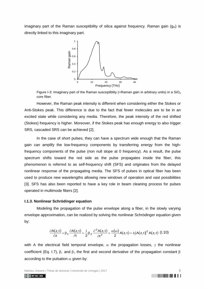
Mathieu Jossent | Thèse de doctorat | Université de Limoges | 2017 6
imaginary part of the Raman susceptibility of silica against frequency. Raman gain (gR) is
directly linked to this imaginary part.
Figure I-3: Imaginary part of the Raman susceptiblity (=Raman gain in arbitrary units) in a SiO2
core fiber.
However, the Raman peak intensity is different when considering either the Stokes or
Anti-Stokes peak. This difference is due to the fact that fewer molecules are to be in an
excited state while considering any media. Therefore, the peak intensity of the red shifted
(Stokes) frequency is higher. Moreover, if the Stokes peak has enough energy to also trigger
SRS, cascaded SRS can be achieved [2].
In the case of short pulses, they can have a spectrum wide enough that the Raman
gain can amplify the low-frequency components by transferring energy from the high-
frequency components of the pulse (non null slope at 0 frequency). As a result, the pulse
spectrum shifts toward the red side as the pulse propagates inside the fiber, this
phenomenon is referred to as self-frequency shift (SFS) and originates from the delayed
nonlinear response of the propagating media. The SFS of pulses in optical fiber has been
used to produce new wavelengths allowing new windows of operation and vast possibilities
[3]. SFS has also been reported to have a key role in beam cleaning process for pulses
operated in multimode fibers [2].
I.1.3. Nonlinear Schrödinger equation
Modeling the propagation of the pulse envelope along a fiber, in the slowly varying
envelope approximation, can be realized by solving the nonlinear Schrödinger equation given
by:
t,zAt,zAit,zA
2t
t,zA
2
i
t
t,zA
z
t,zA 2
2
2
21
(I.10)
with A the electrical field temporal envelope, the propagation losses, the nonlinear
coefficient (Eq. I.7), and the first and second derivative of the propagation constant
according to the pulsation given by:
0
0.2
0.4
0.6
0.8
1
0 10 20 30 40
Frequency (THz)
Ram
an
ga
in

Mathieu Jossent | Thèse de doctorat | Université de Limoges | 2017 7
d
dnn
c
1
d
n2d
d
d1
(I.11)
2
2
2
3
2d
nd
c2
(I.12)
Equations I.12 and I.13 allow the definition of two key parameters in optical fibers: the
group velocity (vg = 1/1 = c/ng with ng the refractive index seen by the pulse called the group
index) which represents the pulse envelope velocity, and the group velocity dispersion
(chromatic dispersion: 22C c2D ) which is responsible for temporal broadening
during the propagation. In our case, optical fibers are electromagnetic waveguides. The
guided electromagnetic field has a peculiar distribution over the plan orthogonal to the
propagation axis depending on the boundary conditions at the core-cladding interface and
due to its cylindrical symmetry. This distribution is caracterized by a group of electromagnetic
modes called Lineary Polarized modes (LPnm) which are composed by linear combination of
pure electromagnetic modes. Those modes ‘see’ the waveguide with a different refractive
index and therefore propagates at different speeds. At a given wavelength, a mode
propagates at speed v allowing the definition of its effective index (neff) given by:
WMeff nnvcn (I.13)
with c the celerity, nM the material refractive index (taken to be the cladding refractive index)
and nW the refractive index contrast in the waveguide. Depending on the considered guided
mode, the effective index can present different slope variations hence different dispersion
(D). When considering a mode of an optical fiber, Equation I.13 can be written as:
2
eff2
eff
2
2 nn2
c
22D (I.14)
MW2
M02
22
W02
2DD
nkc2nkc2D
(I.15)
The dispersion of a mode propagating in a fiber can hence be written as the sum of two
contributions: the waveguide dispersion (DW) and the material dispersion (DM). DM is fixed by
the glass matrix, here silica (Figure I-4). DW can be adjusted by optimizing the refractive
index profile (RIP) of a fiber.

Mathieu Jossent | Thèse de doctorat | Université de Limoges | 2017 8
Figure I-4: Silica dispersion curve calculated by Sellmeier series from [4]. Dispersion values at
commonly used lasing wavelengths: Ytterbium 1.03 µm (blue), Erbium 1.55 µm
(green) and Thulium 1.9 µm (red).
The waveguide contribution to dispersion is strongly dependent to the radial field distribution
according to wavelength and can be expressed as follows:
0
22
0
2
W rdrdr
)r(dE
d
drdr
dr
)r(dED (I.16)
The waveguide dispersion dependence of the fundamental mode is weak as its radial field
distribution varies slowly from 1 to 2 µm. Therefore, the dispersion of the fundamental mode
is close to that of silica. The lower the waveguiding effect, the closer the chromatic dispersion
is to the material dispersion. This is especially the case in large effective mode area fibers,
where waveguiding effects on dispersion are negligible.
In pulsed regime, it is useful to define another characteristic length called the
dispersion length:
2
20
D
TL
(I.17)
with T0 the duration at e1 of the pulse envelope. For a Gaussian pulse, the full width at half
maximum intensity (FWHMi) relates to T0 by 0FWHMi T2ln2T . LD is the distance at which
the duration of a Gaussian pulse is multiplied by 2 . As an example, let us consider a
250 fs (TFWHMi) Gaussian pulse centered at the wavelength of 1.9 µm propagating in a
single mode fiber (SMF). At 1.9 µm, the chromatic dispersion of a SMF is of 42 ps/(nm.km)
(2≈-8.10-26 s²/m). The calculated value of the dispersion length LD is roughly 0.6 m which is
at least three times lower than the length of commonly used fiber amplifiers. Therefore, the
impact of chromatic dispersion will not be negligible.
-60
-40
-20
0
20
40
60
0.9 1 1.1 1.2 1.3 1.4 1.5 1.6 1.7 1.8 1.9 2 2.1
Wavelength (µm)
Dis
pe
rsio
n (p
s/(
nm
.km
))
ThuliumErbiumYtterbium
-34
+22
+42

Mathieu Jossent | Thèse de doctorat | Université de Limoges | 2017 9
I.2. Generalized nonlinear Schrödinger equation
Equation (I.10) describes the propagation of an optical pulse in single-mode passive
fibers. It includes the effects of fiber loss through , group delay through , chromatic
dispersion through and fiber nonlinearities through . The group velocity dispersion can
either be positive or negative depending on whether the wavelength is shorter or longer than
the zero-dispersion wavelength D of the considered mode In the anomalous-dispersion
regime ( 0D02D ) the fiber can support optical soliton which will be
introduced later. Although this propagation equation allowed explaining a large number of
nonlinear effects, it needs modification in order to include other experimental conditions.
Here, neither Raman-induced self-frequency shift nor the gain impact are included. The
inclusion of these effects leads to the generalized propagation equation:
T2
02kk
kkk
'dt'tT,zA'tRT,zAT
i1iT,zA
2
,zG
t
T,zA
!k
ii
z
T,zA
(I.18)
where the chromatic dispersion in expressed as a Taylor expansion of the propagation
constant about the pump wavelength, G stands for the fiber gain and loss depending on
wavelength and fiber length, includes the optical Kerr effect, Ti 0 refers to the
inclusion of self-steepening which reduces the velocity at which the peak of the ultra-short
pulse propagates leading to an increasing slope of the trailing part of the pulse, the integral is
the delayed Raman response accounting for SFS. This equation includes the impact of 1 by
using a co-moving time frame moving at the group velocity ( ztT 1 ).
When considering pulses propagating near the zero-dispersion wavelength D (2≈0)
or for pulses having temporal width below 1 ps [1], the third order dispersion parameter has
an impact. This phase term induces a temporal dissymmetry onto the pulse limiting its
subsequent compressibility.
I.2.1. Modeling the propagation of short pulses in optical fibers
A convenient way to solve the GNLSE (Eq. I.18) is a pseudo-spectral model referred
to as the symmetric split-step Fourier method. It assumes dispersion and nonlinear effects
act independently over a short piece of fiber. It is practical to use equation (I.19) as:
ANDz
A
(I.19)
Mathieu Jossent | Thèse de doctorat | Université de Limoges | 2017 10
where Ď is the differential operator representing the dispersion and gain/absorption in a
linear medium and Ň is the nonlinear operator ruling all the nonlinear effects on pulse
propagation. These operators are given by:
2kk
kkk
2
,zG
t!k
iiD
(I.20)
T2
0
'dt'tT,zA'tRT
i1iN
(I.21)
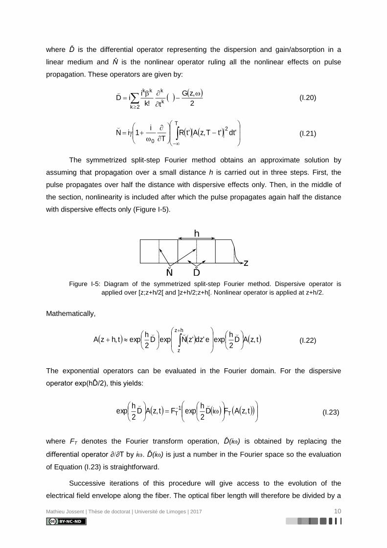
The symmetrized split-step Fourier method obtains an approximate solution by
assuming that propagation over a small distance h is carried out in three steps. First, the
pulse propagates over half the distance with dispersive effects only. Then, in the middle of
the section, nonlinearity is included after which the pulse propagates again half the distance
with dispersive effects only (Figure I-5).
Figure I-5: Diagram of the symmetrized split-step Fourier method. Dispersive operator is
applied over [z;z+h/2[ and ]z+h/2;z+h[. Nonlinear operator is applied at z+h/2.
Mathematically,
t,zAD2
hexpe'dz'zNexpD
2
hexpt,hzA
hz
z
(I.22)
The exponential operators can be evaluated in the Fourier domain. For the dispersive
operator exp(hĎ/2), this yields:
t,zAFiD2
hexpFt,zAD
2
hexp T
1T
(I.23)
where FT denotes the Fourier transform operation, Ď(i) is obtained by replacing the
differential operator ∂∂T by i. Ď(i) is just a number in the Fourier space so the evaluation
of Equation (I.23) is straightforward.
Successive iterations of this procedure will give access to the evolution of the
electrical field envelope along the fiber. The optical fiber length will therefore be divided by a

Mathieu Jossent | Thèse de doctorat | Université de Limoges | 2017 11
fair amount of intervals. In order to lower errors and gain in accuracy, the step h must be at
least two orders of magnitude lower than the shortest characteristic length. Depending on the
dispersion regime, several types of pulses can be found while numerically solving the
GNLSE. In the following, I will introduce two kinds of pulses namely soliton and similariton
which can exist in anomalous and normal dispersion regimes respectively. Those
explanations are adapted from Liu’s thesis [5].
I.2.2. Pulse in the anomalous dispersion regime: Solitons
I.2.2.1. Soliton theory
Soliton pulses are formed thanks to a balance between the nonlinear phase induced
by the Kerr effect and the anomalous dispersion. It maintains its shape and energy along the
propagation once it is formed. It has many solutions for each integer value of the soliton
number N defined as
22
00 /TPN (I.24)
High order solitons correspond to N>1. Fundamental N = 1 soliton is a solution of the
equation (I.25) of the form (I.26):
AAit
A
2i
z
A 2
2
22
(I.25)
2/izexpT/t sechAt,zA 00 (I.26)
If this solution is injected into the GNLSE, we obtain a simple relation between the
pulse parameters and the system parameters called the soliton area theorem:
02T TE (I.27)
According to Equation (I.27), the soliton energy is clamped by balancing nonlinearity and
dispersion. When considering a fundamental soliton centered at 1.9 µm wavelength with
250 fs pulse duration propagating in standard fibers with parameters close to those of
SMF-28 (8.2 µm core diameter, D = 42 ps/(nm.km)), the obtained energy is around 0.7 nJ. In
this configuration, LNL and LD are equal showing the required balance between nonlinearities
and dispersion to maintain a fundamental soliton. A first approach used to increase the
energy of solitons relies on the use of large mode area gain fiber with reduced nonlinear
coefficient. For example, Horton and co-workers [6] used 360 fs pulses containing 500 nJ
of energy centered at 1.55 µm at a repetition rate of 1 MHz to seed a rod-type fiber
presenting 2300 µm² of Aeff. Taking advantage of the soliton Raman self-frequency shift, the
output pulses presented duration of 65 fs centered at 1.675 µm containing 67 nJ of energy.
Mathieu Jossent | Thèse de doctorat | Université de Limoges | 2017 12
I.2.2.2. Soliton laser
The fundamental soliton has the property of maintaining its shape along the fiber once it is
formed and can withstand strong perturbations, such as gain and loss. Solitons were
observed in laser oscillator [7]. Temporal breathing in the laser cavity was also shown to be
effective in increasing the pulse energy [8], [9].
In 2013, a high-energy dissipative soliton oscillator based on a single mode Erbium
doped fiber was reported [9]. Wang and coworkers achieved the net normal dispersion by
introducing a dispersion compensating fiber producing high normal dispersion and a highly
Erbium doped normally dispersive active fiber while all other components and fibers were
exhibiting anomalous dispersion. As in [8], the active core was smaller compared to the other
fiber pieces to produce SPM and achieve normal dispersion. The mode locking was realized
by resonant saturable absorber mirror which induces spectral filtering narrower than the
erbium gain bandwidth. The oscillator output pulses carried 7 nJ of energy in 10 ps at a
repetition rate of 35 MHz. Those pulses could be compressed down to 640 fs assuming a
Gaussian pulse shape.
Unfortunately, single mode Thulium doped fibers present high anomalous dispersion
and reaching the dissipative soliton regime in an anomalous dispersion gain media is quiet
challenging. Tang and coworkers have tried to transpose this regime around the wavelength
of 2 µm [10] by adding ultra high numerical aperture (UHNA) fibers in the cavity. UHNA fibers
come with small cores to keep a single mode behavior and therefore produce normal
dispersion in the anomalous dispersion region of silica. In their setup, the mode locking was
assured by NPE. After fine tuning the lengths of the UHNA fiber, they manage to obtain
output pulses carrying 8.3 nJ of energy in ~3 ps at a repetition rate close to 20 MHz. Those
pulses could be compressed down to 150 fs by a 65% efficiency compressor producing 36
kW peak power. The chirp of the pulses was less than the cavity group delay dispersion
which is a feature of self-similar evolution and not dissipative solitons [11].
I.2.3. Pulse in the normal dispersion regime: Similaritons
I.2.3.1. Similariton theory
Similariton is an asymptotic wave-breaking free solution of the GNLSE in normal
dispersion regime with gain (Equation I.28) identified by Fermann and coworkers [12]. Such
pulses present a parabolic intensity profile and a quadratic phase (Equation I.29-30). This
pulse propagates self similarly maintaining its parabolic shape. It is subject to exponential
scaling of its amplitude, temporal and spectral widths (Figure I-6). To generate those pulses
nonlinear effects are to be predominant over dispersion. The generated second order phase
has to come mostly from SPM in order to get a spectral bandwidth of some tens of

Mathieu Jossent | Thèse de doctorat | Université de Limoges | 2017 13
nanometers. Therefore LNL will be much shorter than LD. The envelope, phase and duration
as functions of the position along the fiber are given by Equation (I.28) to (I.30).
t,ziexp)zT/t1zAt,zA2
00 for |t| ≤ T0(z) (I.28)
22
200 t6/zg)z(Azg2/3t,z (I.29)
3zzgexpE2zg3zT31
IN31
232
0
(I.30)
g(z) is the distributed gain coefficient, EIN the initial pulse energy and 0 is an arbitrary
constant. For an amplifier with constant gain, any kind of pulse is to converge to this solution
if the initial condition (mainly energy) is close enough.
Figure I-6: Illustration of self similar evolution of the temporal (left) and spectral (right) shapes
of a similariton along its amplification.
The maximal energy Ê that an amplified similariton can contain is equal to:
eff
32
2
AD
gn8
cΕ̂ (I.31)
with the full spectral bandwidth and g the distributed gain in Np/m. To increase the
energy, one can increase Aeff or operate the amplifier at high normal dispersion. If the energy
within the pulse becomes greater than what is predicted by Equation I.31, the pulse will not
be a similariton anymore nor will it be compressible to its Fourier limit. Figure I-7 shows the
energy scalability enabled by similaritons according to the dispersion for four different
effective areas spanning from 100 to 400 µm². These curves were calculated with a
distributed gain g = 1.9 Np/m, a full spectral bandwidth of 105 nm centered at 1.9 µm.

Mathieu Jossent | Thèse de doctorat | Université de Limoges | 2017 14
Figure I-7: Calculated maximal extractible energy, before wavebreaking, of an amplified
similariton centered at 1.9 µm as a function of the absolute value of the dispersion
coefficient for various modal effective areas.
It appears clearly that the maximum extractable energy before wavebreaking can be very
high thanks to the temporal breathing in the amplifier. In the following, I will use a figure of
merit (FOM) to easily compare the fiber. This FOM is directly linked to the energy a
similariton propagating in the fiber and is given in Equation (I.32):
effADFOM (I.32)
Commercially available fibers providing normal dispersion around 2 µm such as the UHNA
series from Nufern (D = -55 ps/(nm.km) and Aeff = 18 µm²) present a FOM of 1 femtosecond
and will be a base for comparison.
I.2.3.2. Similariton laser
Amplified similaritons have a pulse duration and a spectral bandwidth which are both
broadening along the propagation. Hence, the output pulse can reach shorter durations
compared to the input pulse and more energy can be stored within the pulse. A useful
feature of these pulses is that the chirp of self-similar pulses is linear. The pulse can be
easily compressed to the Fourier-transform limit by passing through a dispersion
compensating line. The parabolic amplification intrinsically produces broadband spectrum
without wave breaking. They are very sensitive to phase terms of order above two: gain
bandwidth, third order dispersion of the amplifying fiber and of the output compressor and
SPM. However, some studies shown that third order phase terms could be compensated by
SPM when fine tuning the amplifier gain [13]. For rare-earth gain media emitting in the
anomalous dispersion region of silica (>1.3 µm), it is difficult to achieve parabolic
amplification. The commonly used way to produce normal dispersion in an Er- or Tm-doped
fiber is to shrink down the core diameter. This comes with a reduced Aeff and increased
0
5
10
15
20
25
30
35
40
45
50
50 100 150 200 250 300 350 400 450Dispersion |D| [ps/(nm.km)]
En
erg
y Ê
[µJ]
400 µm²
300 µm²
200 µm²
100 µm²

Mathieu Jossent | Thèse de doctorat | Université de Limoges | 2017 15
nonlinearity, hence less room for energy scaling. Nevertheless, oscillators delivering pulses
presenting self-similar features have been reported [12]–[15]. Peng and coworkers
demonstrated an all-fiber similariton oscillator using 1.3 m of a small core Erbium doped fiber
producing -51 ps/(nm.km) at 1.55 µm. In order to meet a cavity resonance, which is
contradictory with an endlessly broadening similariton, 2.7 m of anomalously dispersive
single mode fiber were used to impose temporal breathing. The mode-locking was realized
by means of NPE in the ring cavity. The output coupler was placed before the piece of
singlemode fiber so as to extract uncompressed pulses. This oscillator delivers 700 fs pulses
with a spectral bandwidth of 20 nm containing 0.13 nJ of energy at a repetition rate of
47.6 MHz.
I.3. Ultrafast high power amplifiers
I.3.1. High energy chirped pulse amplifier
The chirped pulse amplification has first been proposed by Strickland and Mourou
[18] and relies on limiting the Kerr effect by using pulses with low peak power. The pulse is
temporally stretched before amplification and recompressed afterwards. The peak power is
therefore minimized along the amplification. In order to realize the stretching and
compression steps, dispersive components generating second order spectral phase are
required. On one hand, singlemode fibers and Bragg gratings (fiber or bulk) are commonly
chosen to stretch the pulse to a few hundreds of picoseconds [18], [19], whereas for few
nanoseconds pulses dispersive lines with diffraction gratings are used [1]–[3]. In those
conditions, it is possible to decrease the peak power by a factor equal to the stretching
factor, around 104 in [20]. Furthermore, the sign and value of the chromatic dispersion in the
amplifier does not matter anymore. On the other hand, the compression line must
compensate the stretcher but also the dispersion and nonlinear phase produced by the
amplifier. Let us consider a CPA scheme as depicted in Figure I-8 taken from [21]. The
general setup, before the last stage of amplification, is composed by a femtosecond oscillator
at a high repetition rate (MHz) delivering low average power (milliwatts [21] to Watt [20]) and
one or two stages of preamplification to increase the average power. In order to reach high
energy, hence high peak power after compression, it is compulsory to decrease the repetition
rate of the input pulses of the last stage amplifier. To do so, a pulse picker, commonly
realized with an acousto-optic modulator as in Figure I-8, is used.

Mathieu Jossent | Thèse de doctorat | Université de Limoges | 2017 16
Figure I-8: Experimental setup of a CPA [21]. (AOM: Acousto-optic modulator, PCF: Photonic
crystal fiber, LPF: Large pitch rod-type fiber).
To obtain highly energetic pulses with a high peak power, the repetition rate must be low
(kHz range) [19]–[21]. The fiber core of the high power amplifier must be as large as possible
to avoid any nonlinear effect.
Very recently, the record peak power of 1.74 GW has been set by Gaida and
coworkers [21] in a Thulium-doped large-pitch fiber by transposing the technique from 1 µm
to 2µm. The seed laser was a mode-lock thulium doped fiber laser emitting around 0.5 nJ
pulses at a repetition rate of 33 MHz. The pulses were then temporally stretched to 0.6
nanoseconds. The repetition rate was decreased twice to reach 61 kHz. The two
preamplifiers allowed reaching an energy pulse of 0.8 µJ to seed the amplifier. The main
amplifier was composed of 1.15 m long Thulium-doped large-pitch rod-type fiber presenting
an 81 µm core diameter. Backward propagating pump was guided by an airclad. The output
pulse duration was 800 ps containing 570 µJ. Due to the transmission efficiency of the
compression line, the energy contained in recompressed 270 fs pulses was 470 µJ. The
average power was 28.7 W and the peak power was 1.74 GW. Limitations arose from the
fact that a large bandwidth of the Thulium emission range overlaps with water absorption
lines. To avoid those absorption lines, the authors shifted the central spectrum above 1.95
µm and operated in a climate chamber with reduced humidity. The thulium cross sections
being higher in the water absorption bandwidth, differential losses have to be put on shorter
wavelength to obtain proper amplification above 1.92 µm.
As said earlier chirped pulse amplification is a linear amplification. Experimentally
those amplifiers allow reaching high peak power. This will have direct influence over the
pulse phase and on the extracted pulse peak power. When considering power amplification,
the non-uniformity of the gain over the considered bandwidth will lead to a pulse asymmetric
spectral profile and phase which are difficult to compensate in the last step of compression.
Mathieu Jossent | Thèse de doctorat | Université de Limoges | 2017 17
The amplified spectrum can be quite different compared to the input spectrum. This can be
explained by different phenomena.
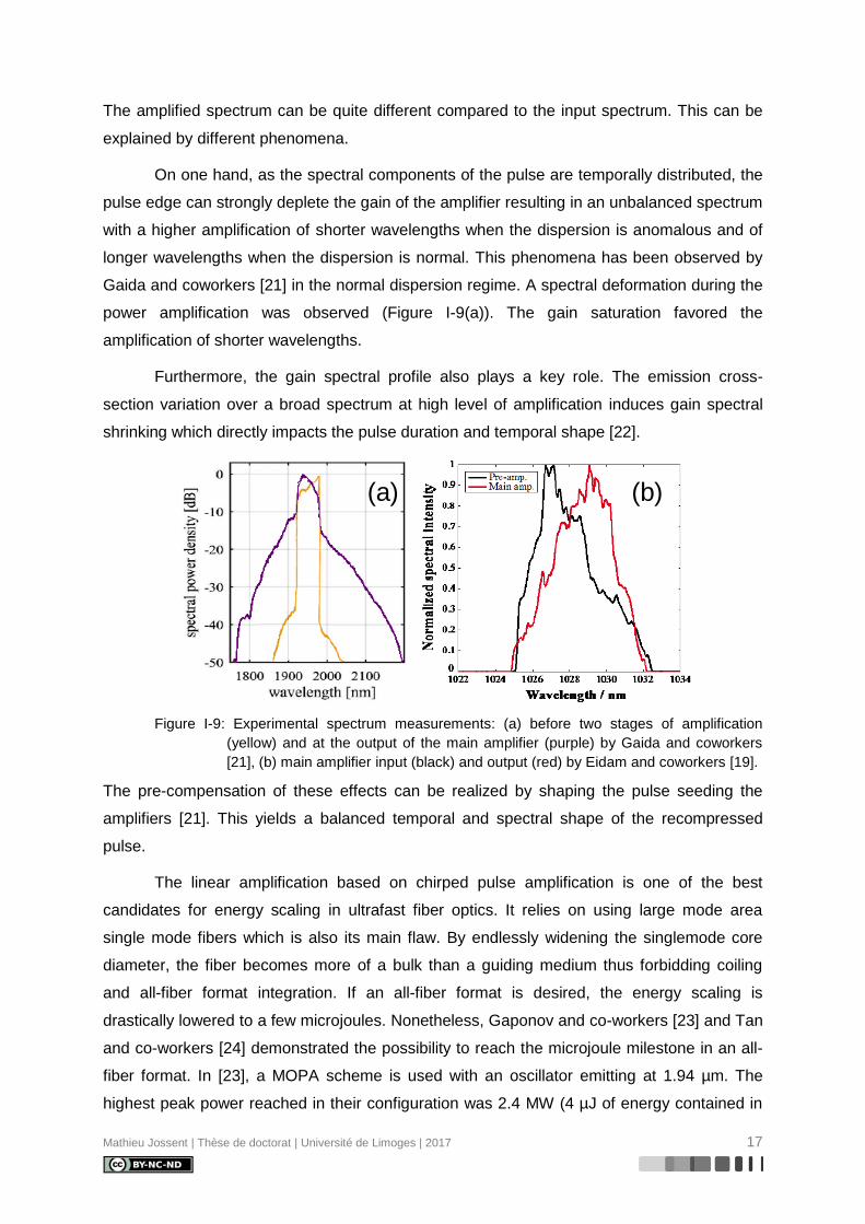
On one hand, as the spectral components of the pulse are temporally distributed, the
pulse edge can strongly deplete the gain of the amplifier resulting in an unbalanced spectrum
with a higher amplification of shorter wavelengths when the dispersion is anomalous and of
longer wavelengths when the dispersion is normal. This phenomena has been observed by
Gaida and coworkers [21] in the normal dispersion regime. A spectral deformation during the
power amplification was observed (Figure I-9(a)). The gain saturation favored the
amplification of shorter wavelengths.
Furthermore, the gain spectral profile also plays a key role. The emission cross-
section variation over a broad spectrum at high level of amplification induces gain spectral
shrinking which directly impacts the pulse duration and temporal shape [22].
Figure I-9: Experimental spectrum measurements: (a) before two stages of amplification
(yellow) and at the output of the main amplifier (purple) by Gaida and coworkers
[21], (b) main amplifier input (black) and output (red) by Eidam and coworkers [19].
The pre-compensation of these effects can be realized by shaping the pulse seeding the
amplifiers [21]. This yields a balanced temporal and spectral shape of the recompressed
pulse.
The linear amplification based on chirped pulse amplification is one of the best
candidates for energy scaling in ultrafast fiber optics. It relies on using large mode area
single mode fibers which is also its main flaw. By endlessly widening the singlemode core
diameter, the fiber becomes more of a bulk than a guiding medium thus forbidding coiling
and all-fiber format integration. If an all-fiber format is desired, the energy scaling is
drastically lowered to a few microjoules. Nonetheless, Gaponov and co-workers [23] and Tan
and co-workers [24] demonstrated the possibility to reach the microjoule milestone in an all-
fiber format. In [23], a MOPA scheme is used with an oscillator emitting at 1.94 µm. The
highest peak power reached in their configuration was 2.4 MW (4 µJ of energy contained in
(a) (b)

Mathieu Jossent | Thèse de doctorat | Université de Limoges | 2017 18
1.6 ps). In [24], the pulses originated from an Er-doped fiber amplifier were Raman-shifted
around 1.97 µJ before entering two stages of amplification. The use of high pump power
(over 140 W at 793 nm) in the last stage allowed reaching 3 MW peak power for
recompressed pulses (241 fs of pulse duration containing 700 nJ of energy). These results
represent the benchmark for our aimed parabolic amplification
I.3.2. High energy parabolic amplifier
In the parabolic amplifier, the goal is to take advantage of nonlinear effect by
exploiting an auto-similar propagation regime. The generated second order phase has to
mostly come from SPM. The goal is to get a spectral bandwidth of some tens of nanometers.
Therefore, LNL is shorter than LD. A transform-limited ultrashort pulse propagating in such an
amplifier will have its temporal and spectral shapes tend towards parabolic profiles [12]. The
pulse will therefore be a similariton as described in I.2.3.
The work realized by Zaouter and coworkers in 2008 emphasized the benefits and
drawbacks of parabolic amplification in an Ytterbium doped large mode area photonic crystal
rod-type fiber. The amplifying fiber was 85 cm long and presented an 80 µm core diameter.
This single mode fiber presented an effective modal area of 3850 µm². The calculated
nonlinear length was a hundred times lower than the dispersion length. The active fiber was
backward pumped. It was directly seeded by an ultrafast oscillator delivering 330 fs pulses
with a spectral bandwidth of 3.9 nm containing 170 nJ of energy at a repetition rate of 10
MHz. A specifically designed compressor and adjusted pulse energy allowed the generation
of short pulses while keeping a high quality temporal shape. Third order phase management
has been optimized through those parameters. The best performances, in terms of peak
power (16 MW), were obtained for pulses of 70 fs with a limited energy of 1.25 µJ without
lowering the repetition rate. The amount of power in the main peak was 89%. The pulse
duration was limited by the spectral filtering imposed by the compressor.
At 1.55 µm Peng and coworkers [15] used an Erbium doped fiber with -51 ps/(nm.km)
dispersion, seeded by the similariton oscillator described in [25]. The amplifier was forward-
and backward core-pumped. At the output of this nonlinear amplifier, the output pulse was
compressed using standard singlemode fiber to keep an all-fiber format. The 113 fs duration
pulse contained 4.1 nJ (54 kW peak power). Since a similariton was amplified the pulse had
a pedestal-free temporal shape and a smooth spectrum. According to the authors, the only
limitation to power scaling was due to the available pump power of the amplifier.
Table I-1 summarizes the different references that have been focused on.

Mathieu Jossent | Thèse de doctorat | Université de Limoges | 2017 19
Table I-1: References performances summary. In green are underlined the aimed
performances. In red are represented the unwanted charateristics
Up to now, to our best knowledge, there is no demonstration of similaritonic
amplification at 2 µm. In this thesis, I’ve tried to pave the way to this demonstration by
designing gain fibers with normal dispersion. This is the objective of the second chapter of
this manuscript.
I.4. Conclusion
Over the past years, energy scaling of ultrashort pulses in all-fiber format lasers has
been mostly realized via mode area tailoring, culminating in the use of parabolic amplification
(dissipative solitons) in all-normal dispersion (ANDi) lasers at 1 µm, where silica exhibits
normal dispersion. This attractive amplification regime is prohibited at 2 µm due to large
anomalous dispersion of silica. According to Eq. (I-31) the best all-fiber amplifier at 2 µm
would need a special Tm-doped fiber with both increased D and Aeff. It is impossible to
design a single mode fiber with large mode area and high –D at 2 μm since waveguiding
effects are inhibited by nature in large mode area singlemode fibers. On the other hand,
Poole et al., from the Bell Labs [26], showed that high-order modes in optical fibers could be
used for dispersion control. These modes might exhibit high –D and large mode area near
their respective cut-offs. They are therefore suited to energy scaling at 2 µm via parabolic
amplification. To our best knowledge, no rare-earth doped version of this design has been
produced to date.
The goal of this thesis is to pave the way towards the demonstration of parabolic
amplification at 2 µm. To achieve this goal, the manuscript is organized in three chapters.
First, a fiber gathering all attributes necessary to initiate parabolic amplification at 2 µm (gain,
normal dispersion and large mode area) designed at XLIM and fabricated by MCVD at
IRCICA/PhLAM is presented. The second chapter reports on the first, to our knowledge,
spatial mode converter efficient over a broad bandwidth from 1.55 µm to 2 µm. The device
was designed, fabricated and characterized at XLIM. In the second chapter, I also present a
Reference Gaida [21] Gaponov [23] Tan [24] Zaouter [13] Peng [15]
Amplifier architecture Tm CPA Tm CPA Tm CPA Yb Similariton Er Similariton
Year 2016 2016 2016 2008 2012
Eout [µJ] 470 4 0.7 1.25 0.0041
tout [ps] 0.27 1.6 0.241 0.07 0.113
Peak power [MW] 1740 2.5 3 16 0.54
Repetition rate [kHz] 61 92 34800 10000 47600
Amplifier fiber type Rod All-fiber All-fiber Rod All-fiber
Amplifier fiber core diameter [µm] 81 10 25 80 ~3
FOM [fs] 130 1.5

Mathieu Jossent | Thèse de doctorat | Université de Limoges | 2017 20
source of ultrashort pulses tunable between 1.8 and 2.1 µm that has been designed, built
and characterized at XLIM in order to seed the nonlinear amplifier. In the third chapter, a
numerical study of the potential of the designed fiber to achieve high energy similariton is
presented.

Mathieu Jossent | Thèse de doctorat | Université de Limoges | 2017 21
Chapter II. Modeling of a dispersion tailored few mode fiber
Similariton amplification was achieved in singlemode silica-based fibers at 1.55 µm.
However, the energy contained in the pulse is three orders of magnitude lower than that
achieved at 1 µm. This is mostly due to the small-core design used to achieve normal
dispersion in the gain media. Following Equation I.31, the higher the dispersion and/or the
effective mode area, the higher the energy. However, the way to generate normal dispersion
in single mode fiber is to reduce the fiber core and increase the core refractive index hence
reducing the effective mode area. New ways of generating both high normal dispersion and
high effective mode area values in silica-based fibers are required to enable power scaling
based on auto-similar amplification at wavelengths where silica exhibits anomalous
dispersion.
In the early 90’s, the emergence of erbium-doped fiber amplifiers operating in the
third telecommunications window allowed information transmission over thousands of
kilometers in single mode fibers without any electronic regeneration. Dispersion
compensation had quickly been required when considering short pulses propagating in a
dispersive media over such long distances. A way to compensate silica dispersion in the
erbium C-band has been proposed by Poole and coworkers [26] from Bell Labs by taking
advantage of the fact that a higher order mode approaching its cutoff wavelength would
produce high normal dispersion. They used a two-mode fiber guiding the fundamental LP01
and the first higher order mode, namely the LP11. The large waveguide dispersion of LP11
near its cutoff arises from the strong wavelength dependence of its electric field distribution
(Equation I.16). When a higher order mode approaches its cutoff, it will spatially leak away
from the core to the cladding. The overlap of the LP11 with the core decreases as the
wavelength is increased toward cutoff. The generated dispersion will be negative since the
core has a higher refractive index than the cladding. If the mode would leak from a low
refractive index media to a high refractive index media, the dispersion would be positive. By
doing so, not only has the generated dispersion the required sign to compensate the silica
dispersion, but the effective mode area of the mode inherently increases as it approaches
the cutoff. The experiment conducted by Poole and coworkers relied on the use of two
distinct two-mode fibers. The first one had a cutoff wavelength of 1.93 µm and the specificity
of matching the effective indices of the LP01 and the LP11 around 1.55 µm. This fiber was
used to favor the conversion from the fundamental mode to the high order mode. The other
fiber had a cutoff wavelength of 1.64 µm and was used as the dispersion compensating fiber.
Mode conversion was realized by applying strain on the first fiber by a gold wire wrapped
around the bare fiber. The dispersion measured at 1.55 µm was -228 ps/(nm.km) for the LP11
Mathieu Jossent | Thèse de doctorat | Université de Limoges | 2017 22
and +22 ps/(nm.km) the LP01. The overall loss of the device comprising mode converter and
different splices was 0.36 dB. Pulses at carrier wavelengths from 1533 nm to 1551 nm could
be recompressed in that way.
Higher mode (HOM) fibers were also used for their ability to propagate large single
modes. Ramachandran and coworkers [27] demonstrated the excitation and propagation
over 5 meters of a LP07 mode in a HOM fiber. The mode exhibits 2100 µm² effective area
and anomalous dispersion of +35 ps/(nm.km). The HOM fiber design was based on two
concentric waveguides. The center core was singlemode. The surrounding core of around
80 µm diameter guides HOMs up to at least the LP07. The mode conversion between the
fundamental LP01 of the center core to the LP07 of the multimode core was ensured by long
period gratings. This HOM fiber was used as a dispersion compensation element in an Er-
doped fiber laser. The active single mode Er-doped fiber exhibits normal dispersion provided
by a small–core design. The amplifier was seeded by femtosecond pulses containing 17 pJ
of energy at a repetition rate of 46 MHz. The output pulses were strongly chirped due to the
normal dispersion regime of the amplification and carried 14 nJ of energy. After 5 m of
propagation in the higher order mode of the HOM, the pulses were compressed to 152 fs
presenting 61 kW peak power. As the HOM fiber presented a LD/LNL of 1 some SPM and
spectral features were expected during the pulse propagation. The spectral shape of the
input pulse was somewhat preserved along the HOM fiber and even after the maximum
pulse compression. This method allowed reaching rather high peak power without provoking
wavebreaking. Indeed, the authors replaced the HOM fiber by a SMF and the spectrum was
strongly broadened.
Another type of higher order mode fibers was used as a gain media to improve the
energy scalability of amplifiers. Peng and co-workers [28] used a 2.65 m long Er-doped HOM
fiber propagating several higher order modes. The LP0,11 of this fiber presented a 6000 µm²
effective area. The conversion to and from this higher order mode was realized with two
broadband (approximately 150 nm around 1.525 µm) LPGs for both the pump Raman laser
at 1.48 µm and signal at 1.553 µm with nearly 99% efficiency. The conversion at the pump
wavelength allowed maximum pump-signal overlap, high pump absorption and reduced
amplifier length. The input pulses presented less than 500 fs duration containing 0.6 µJ at a
repetition rate of 25 kHz. They could be amplified from 16 µJ to 595 µJ in the HOM amplifier
without any spectral distortion. The compression line had a 50% efficiency but allowed to
reach less than 500 fs pulse duration thus producing over 600 MW peak power. The mode at
the output of the HOM amplifier was converted back in a coreless fiber with an 8° end cap to
obtain high beam quality. By using a higher order mode in their amplifier the authors proved

Mathieu Jossent | Thèse de doctorat | Université de Limoges | 2017 23
that energy scaling could be realized in these high order modes if extra care is taken in the
mode conversion.
Note that the dispersion-tailored HOM fiber and large-mode-area (gain) HOM fiber,
although named in the same way, are essentially different by design. Up to now, to our
knowledge, there is no dispersion-tailored HOMF exhibiting gain and large mode area.
Tailoring the dispersion and the effective area in a rare-earth-doped high order mode
fiber could open the path towards power scaling in optical fibers, through direct amplification
in normal-dispersion regime.
II.1. Principle of operation
In cylindrically symmetric fibers, it has been shown that the waveguide dispersion DW
originates from the variation of the radial electric field distribution E(r) with wavelength. The
modal contribution to the dispersion can be expressed in a convenient form as:
0
22
0
2
W rdrdr
)r(dE
d
drdr
dr
)r(dED (II.1)
The first term on the right hand side of Eq. (II.1) is always positive whereas the second one
can be either negative or positive depending on the spectral variation of the slope of E(r).
Usually, E(r) spreads out of the core when the wavelength is increased. Thus, dE(r)/dr
decreases whatever r, with increasing wavelength. Consequently the second integral in the
right-hand side is a decreasing function of , leading to a negative second term. Therefore,
the modal contribution to dispersion is usually negative. To increase the value of the negative
dispersion, so as to compensate for the anomalous dispersion of silica it is therefore
necessary to increase the rate of spectral variation of dE(r)/dr. This effect can be obtained in
the vicinity of the cut-off wavelength of a peculiar mode. The fundamental mode has an
infinite cut-off wavelength and is therefore not suitable to this purpose. On the other hand
each high-order mode has finite cut-off wavelength. In Figure II-1, we consider the first
cylindrically symmetric high-order mode, i.e. the LP02 mode, when it is approaching its cut-off.
As the wavelength increases the guided mode tends towards a plane wave in the infinite
cladding medium. The slope dE(r)/dr is strongly changing slightly below cut-off, thus producing
high negative dispersion. This effect corresponds to a strong inflexion in the modal effective
index curve which tends towards the cladding index at the cut-off. According to Eq. (II.1) this
inflexion produces high –DW. Few mode step-index fibers have been designed so that a high-
order mode cuts off in the telecom window ( = 1.56 µm) [26]. The high-order mode
presenting high normal dispersion (-288 ps/nm/km) was used in a dispersion compensating
device or to recompress pulses from a mode-locked laser.

Mathieu Jossent | Thèse de doctorat | Université de Limoges | 2017 24
Figure II-1: Principle of operation of a moderately multimode fiber for dispersion control. Top:
Generic profile of a step-index moderately multimode fiber. Associated LP02
intensity profile. Middle: LP02 mode effective index versus wavelength. Insets show
the field spreading when increases. Bottom: LP02 dispersion versus wavelength.
II.2. Design criteria
A key issue in the design of few mode fibers is which higher order mode the signal is
to propagate in. Since our goal is high normal dispersion values, one could naturally tend to
choose the mode that gives the most desirable dispersion characteristics. However, it turns
out that other design issues limit the choice of mode.
The most important amongst these issues is mode beating, also called multi-path
interference (MPI), that causes pointing instabilities and noise at the output of a laser.
Generally speaking, in order to limit MPI, one should limit the number of guided modes, and
thus the possible interference paths in the few mode fiber. This means that the signal should
propagate in the lowest order mode that still provides the required dispersion characteristics.
For example, as in [26], if we were to select the LP11 mode as the propagation mode, then it
would be possible to design a fiber with only two guided modes (LP01 LP11). On the other
hand, if we were to select the LP03 mode there would have nine guided modes (LP01, LP11,
LP21, LP02, LP31, LP12, LP41, LP22, and LP03). This means that even if the LP03 was to exhibit
particularly attractive dispersion properties, the increased MPI due to the mode coupling to
other modes would be prohibitive. MPI is a measure of mode coupling. Mode coupling will
decrease with increasing difference between the effective indices of two considered modes.
This characteristic of few-mode fiber can be tailored by design of the refractive index profile.
A second important consideration is polarization dependent behavior. Modes that are not
cylindrically symmetric are by nature more susceptible to polarization effects. This effectively
restricts the selection of modes to those with cylindrical symmetry, i.e., LP0m.
The preceding discussion basically means that the LP02 mode is the logical choice for the
propagation mode in few mode fibers for dispersion tailoring. In fact, we will see that with

Mathieu Jossent | Thèse de doctorat | Université de Limoges | 2017 25
proper fiber design this mode also provides the required dispersion properties. Working near
the cut-off is however troublesome. First, any local changes in index will result in cutting-off
the mode at a non-desired wavelength. Second, the dispersion slope is very steep and
cannot be engineered. Third, working close to the cut-off may imply excess bending loss.
This step index RIP hence brings limited flexibility.
II.3. Improved design
Ramachandran [29] has proposed an improved design of such a few mode fiber (see
Figure II-2). The LP02 is the mode of interest. The complex RIP incorporates a central high-
index multimode core, an adjacent down-doped trench and one high-index ring. The ring
confines the LP02 mode and therefore rejects the cut-off wavelength towards longer
wavelengths, hence providing low loss operation in the telecom window. The ring provides a
smooth dispersion variation that allows slope dispersion tailoring. The dispersion magnitude
is tuned by the trench.
Figure II-2: Principle of operation of an improved design of a few mode fiber for dispersion
control. Top: Generic index profile of a few mode fiber. Associated LP02 intensity
profile. Middle: LP02 mode effective index (thick black curve) is a linear combination
of the ‘core’ mode and of the ‘ring’ mode. The inflexion causes high –DW around
the phase-matching point. The effective index of the LP02 is increased above the
silica index ensuring low loss guidance. Bottom: LP02 dispersion versus
wavelength. The additional features (trench, ring) help tailor the dispersion and
dispersion slope.
As shown in Figure II-3(b) very high normal dispersion (–500 ps/nm/km) can be reached in
this fiber design. The high negative dispersion associated with the low dispersion slope can
be useful when considering an application as a parabolic amplifier.

Mathieu Jossent | Thèse de doctorat | Université de Limoges | 2017 26
Figure II-3: (a) LP02 mode profile at the most dispersive wavelength (solid line) in a few mode
fiber (RIP: gray background). (b) Corresponding plot of LP02 dispersion versus
wavelength. λcut-off represents the wavelength at which the LP02 mode leaks in the
cladding [29].
II.4. Modeling towards optimal design
In the following I present the various steps to design few mode fibers in the context of
high-energy amplifiers. I am searching for designs presenting high normal dispersion values,
broad wavelength spectrum, large effective mode area and low multi-path interference. MPI
will be evaluated through the difference in effective index between the desired mode (LP02)
and its nearest neighbor. I have concentrated the study on the three-layer profile shown in
Figure II-4.
Figure II-4: The various parameters of a typical few mode fiber for dispersion control.
The graded index core is defined by n1(r) and r1. n1(r) is given by the following formula:
111
r
r21n)r(n (II.2)
where n1 = n1(0), is the gradient order and is the relative index difference defined by:
214
24
214
nn2
nnn
(II.3)

Mathieu Jossent | Thèse de doctorat | Université de Limoges | 2017 27
where n4 is the cladding index, chosen to be equal to that of pure fused silica. n2 and r2
are the trench parameters. n3 and r3 are the ring parameters.
The profile comprises seven degrees of freedom: three index differences, three thicknesses
and the gradient order. It is therefore very unlikely to find a convenient set of parameters
from nothing. I have therefore considered the RIP from [29] as a seed:
Table II-1: Refractive index profile from [29]
r n
Core 4 2510–3
Trench 2.5 –810–3
Ring 3.5 410–3
I have taken = 6 to match the RIP in [29] and then used the scaling properties of Maxwell
equations to find a suitable RIP operating at 2 µm. Let us consider the original RIP with
parameters n and r, the scaled RIP with n* and r*, and the scale factors a and b are
such that:
nan* (II.4)
rbr * (II.5)
The scalar wave equation for the two index profiles will be the same when the wavelength
is scaled as:
ab* (II.6)
The waveguide dispersion DW then scales according to:
W*W D
b
aD (II.7)
According to Eq. (II.4-7) a nominal RIP can be scaled in index and/or in radius to provide any
dispersion at any wavelength. The scaling rules have also an important practical aspect:
when drawing a fiber during manufacturing, the outer diameter of the fiber as well as all other
transverse dimensions may be altered by altering the drawing conditions. This results in
scaling of the fiber profile, and allows fine tuning of the dispersion properties during
manufacturing.
The original RIP used the deepest trench that can be achieved (n2 = –810–3) [30].
However, IRCICA-PhLAM, our technological partner, is limited to n2 = -410-3. n was then
scaled by a factor a = 1/2 to cope with this technological limitation. The operating wavelength
is then scaled by the inversed squared root of 2. The wavelength of highest –DW is then

Mathieu Jossent | Thèse de doctorat | Université de Limoges | 2017 28
shifted from 1.55 to 1.1 µm. The highest –DW thus becomes –350 ps/(nm.km). I have then
scaled the fiber radii by a factor b = 2 in order to shift the operating wavelength to 2.2 µm.
The highest –DW thus becomes –175 ps/(nm.km). The scaled RIP is given in Table II-2 and
presents a FOM of 34 fs.
Table II-2: Original and scaled RIP for an operation around 2 µm.
Original RIP [29] Scaled RIP
r n n* = 0.5n r* = 2r
Core 4 2510–3 12.510–3 8
Trench 2.5 –810–3 –410–3 5
Ring 3.5 410–3 210–3 7
[µm] 1.55 2.2
D [ps/(nm.km)] –500 –175
This is certainly not the highest –DW that one can achieve with this technique. The scaled
RIP is however a seed for further numerical optimization. In the following we will consider the
scaled RIP as the nominal values. As mentioned above each part of the RIP influences the
dispersion curve. As shown in Figure II-5, the LP01 mode is guided by the core. The LP02 is
mainly guided by the core but is also dependent on the trench and ring parameters. As
shown in Figure II-2, middle, the LP02 is accompanied by the LP03 which results from the
coupling between the ‘core’ LP02 and the ‘ring’ LP01. As shown in the bottom inset of
Figure II-5 it is mainly guided by the ring.
Figure II-5: The various LP0m, in intensity, of a typical few mode fiber for dispersion control with
their effective index position according to the RIP.
First, the LP03 index curve is convex leading to high anomalous dispersion. Second, ne02 and
ne03 are very close. This may lead to MPI. Great care must be taken to cut this parasitic
mode, i.e. keep its effective index close or even below that of silica, while preserving the LP02
mode. Therefore, in order to lower the LP03 guidance, we will have to decrease the influence
of the ring.
The curvature of the effective index is tuned by the coupling strength between the core and
the ring modes. A low coupling strength implies small interaction between the core and the

Mathieu Jossent | Thèse de doctorat | Université de Limoges | 2017 29
ring mode and the curvature of the effective index difference will be high at the phase-
matching point. This is thus accompanied by large dispersion and small bandwidth. Second
the effective index difference ne02-ne03 will be small. A low coupling strength thus means that
both modes are likely to be guided. This situation can be avoided if the core and ring are
close to each other, thus limiting the trench thickness to a few microns.
In order to understand the impact of each index layer and search for optimal parameters, it is
necessary to study each layer separately. I have modified the scaled RIP according to these
general rules. The results are given below.
II.4.1. Impact of the ring
The width of the ring r3 was varied by –50 % to 100 % of the nominal value. Results are
shown in Figure II-6.
Figure II-6: Impact of the ring thickness r3 on the dispersion spectrum.
Figure II-6 depicts the fact that enlarging the ring produces high –DW. Second, the dispersion
spectrum is shifted towards the shorter wavelengths. Enlarging r3 comes down to push
away the fiber cladding. Thus, it strengthens guidance of the LP02 mode. This increase in
dispersion comes with a narrowing of the spectrum in which high –DW can be achieved.
The nominal index difference of the ring n3 nom was then varied by –210-3 to +310–3.
Results are shown in Figure II-7.

Mathieu Jossent | Thèse de doctorat | Université de Limoges | 2017 30
Figure II-7: Impact of the ring index difference n3 on the dispersion spectrum.
The increase in n3 strengthens the LP02 guiding. The slope of the mode effective index is
therefore increased. Thus, it offers access to higher –DW. However, this effect comes also
with a wavelength shift to the shorter wavelengths and a narrowing of the high –DW
spectrum. Moreover, the LP03 waveguidance is also strengthened, leading to possible MPI.
n3 must be kept on the level of n3 nom or below to avoid excess MPI.
The variations in both r3 and n3 offer a wavelength shift and an increase in the dispersion
value. However, increasing n3 too much makes the dispersion slope too high and the
spectrum too narrow. An increased r3 does not affect the dispersion and the wavelength
shift as much as n3. Those shifts have to be taken in consideration when designing the RIP
of the fiber to obtain the desired dispersion at the desired wavelength.
II.4.2. Impact of the trench
I have then studied the impact of the trench. The ring has been removed. First, the
width of the trench r2 was varied by – 50 % to 100 % of its nominal value. Results are
shown in Figure II-8.
Figure II-8: Impact of the trench thickness r2 on the dispersion spectrum.

Mathieu Jossent | Thèse de doctorat | Université de Limoges | 2017 31
Figure II-8 shows that the thicker the trench the deeper the waveguide dispersion near the
cut-off. With an increasing trench width, the LP02 is better guided. Therefore, the slope with
which the effective index arrives at the value of the cladding one is higher. Therefore, it
produces high –DW near the cut-off wavelength. Increasing the trench thickness comes down
to push away the cladding, thus enlarging the index difference between the core and the
trench that serves as a cladding. When a ring is added to the RIP the coupling between the
core and the ring mode is decreased. Therefore producing higher –DW values but narrowing
the dispersion curve. Hence this situation, even if the desired effect on dispersion is
obtained, is not suitable.
The index difference of the trench n2 was then varied from –110-3 to +210–3. Results are
shown in Figure II-9.
Figure II-9: Impact of the trench index difference n2 on the dispersion spectrum.
Figure II-9 depicts the effect of an increased trench depth. The lower the n2 the higher the
-DW near cut-off.
The variations in both r2 and n2 offer high –DW values near the cut-off. However, an
increase in r2 shifts the high –DW value to the shorter wavelengths. Thus it has to be done
to a certain extent. Therefore, we will have to focus on the depth of the trench to obtain high
-DW values. However, the inflexion of the ne02 curve at this point would be higher leading to a
narrow bandwidth.
A summary of the different phenomena met during those simulations is available in
Table II-3.

Mathieu Jossent | Thèse de doctorat | Université de Limoges | 2017 32
Table II-3: Summary of the ring and trench contributions to the dispersion spectrum. (‘+’
stands for an increase).
Ring Trench
n3 + r3 + | n2 | + r2 +
Spectrum shifts
Strongly to the short λ
Slightly to the short λ
| DW | + + + + + + + +
The trends have been used to determine an optimized RIP. The results are shown in
Figure II-10.
Figure II-10: Chromatic dispersion of the designed RIP versus wavelength. Inset: RIP for
improved dispersion. α = 6, n1 = 1510–3
, r1 = 8 µm, n2 = –410–3
, r2 = 4 µm,
n3 = 310–3
, r3 = 8 µm.
The chromatic dispersion is as high as –380 ps/(nm.km) at 1.908 µm (Dmax). The computed
LP02 mode field area for this RIP is of 353 µm² at Dmax. The optimal fiber presents a figure of
merit (DAeff) of 134 fs which is as high as Zaouter’s [13].
II.5. Fabricated passive few-mode fiber
A very first version of the fiber design described above was manufactured by the
MCVD process at IRCICA/PhLAM. Measured RIP and dispersion curve computed for the
LP02 mode taking the actual RIP into account are shown in Figure II-11 (a-b). The high index
ring is lower than expected, thus increasing the sensitivity of the LP02 mode to the curvature.
The trench is not step-like, which is expected to impact on the dispersion spectrum of the
LP02 mode. Despite the discrepancy between the target and the actual RIP, negative
dispersion is obtained around 2 µm.

Mathieu Jossent | Thèse de doctorat | Université de Limoges | 2017 33
Figure II-11: (a) Measured refractive index difference of the passive (blue) few mode fiber.
Black line shows the target RIP. (b) Dispersion curves computed for the two RIPs
shown in (a).
The effective areas were computed at the wavelength of minimum dispersion for both fibers
enabling to calculate the expected FOM. These values are summarized in Table II-4.
Table II-4: Computed dispersion and effective area of the LP02 mode for the target and
manufactured fibers at their respective Dmax.
Fiber Target Manufactured
Dmax (µm) 1.908 1.99
|Dmax| (ps/(nm.km)) -380 -137
Aeff (µm²) 353 398
FOM (fs) 134 55
II.6. Conclusion
It is a real scientific challenge to gather large Aeff and high –D at long wavelengths in
silica fibers since in large core fibers the waveguidance is very weak, leading to negligible
DW. In this section, I have presented a fiber design yielding large mode area and strong
waveguidance effects, leading to high normal dispersion adjustable by design to any
operating wavelength. A few mode fiber maximizing Aeff and |D| around 2 µm has been
designed taking into account the limitation of the MCVD process. Then a passive fiber was
manufactured by the MCVD process. The parameters computed taking the actual RIP into
account are D = -137 ps/(nm.km) and Aeff = 398 µm2 at the wavelength of 1.99 µm in the
fluorescence band of Tm3+ ions.
-5
0
5
10
15
0 10 20
Re
fra
ctive
ind
ex
diffe
rence
(x1
0-3
)
Fiber radius (µm)
Optimal
Passive
(a)
-400
-350
-300
-250
-200
-150
-100
-50
0
1.8 1.9 2 2.1
Optimal
Passive
Dis
pe
rsio
n (p
s/(
nm
.km
))
Wavelength (µm)(b)

Mathieu Jossent | Thèse de doctorat | Université de Limoges | 2017 34
Chapter III. Mode conversion in optical fibers
The use of such optical fibers requires selective excitation of the highly dispersive mode or
mode conversion from the input single mode fiber into the higher order transverse mode of
the few mode amplifying fiber (Figure III-1).
Figure III-1: Scheme of a high-order mode based amplifier. Light propagating in the LP01 mode
of the input fiber is converted to a high normal dispersion high-order mode of a few
mode fiber, the LP02 mode for instance.
The challenge in designing a good spatial mode converter is twofold:
To transfer a maximum fraction of the energy of the input mode into the desired high-
order mode,
To match the conversion bandwidth to the –D spectrum.
Moreover, the modal content of these few mode fibers and how it behaves according to the
excitation conditions has to be thoroughly investigated in order to make the maximum out of
few mode amplifiers.
III.1. Long period gratings with controlled bandwidth
To selectively couple the input LP01 to the desired high-order mode, Poole and
coworkers [26] have used grating coupling. Coupling occurs between two modes when the
grating period sted to match the intermodal beat length given in Equation III.1.
02e01e nn2 (III.1)
This resonant coupling phenomenon has a very narrow bandwidth, on the order of 1 to 3 nm,
thus limiting its use in a pulsed amplifier. However, as demonstrated in [29] the bandwidth
is conversely proportional to the derivative of with respect to the wavelength, i.e. the
group index difference. A detuning parameter ( 25.0 ) directly impacting
the coupling strength between the two modes can be defined. This detuning parameter
allows fine tuning of the grating period. The conversion bandwidth will be the largest as this
parameter reaches zero. Therefore, the spectrum of an LPG can be tailored by adjusting the
refractive index profile (RIP). However, having a large spectrum for the LPG and a tailored
dispersion in this spectrum is quite a technological challenge.

Mathieu Jossent | Thèse de doctorat | Université de Limoges | 2017 35
There are several techniques to write LPGs in optical fibers. The electric-arc
technique [31] is independent of the fiber composition. The arc is 300 µm wide. Therefore the
achievable grating period is longer than 500 µm limiting the index difference Δne to values
under 4×10⁻³ (Δne < 4×10⁻³). Furthermore the electric arc induced by a conventional fusion
splicer is not cylindrically symmetric. It makes it difficult to couple light efficiently in the LP02
mode. The UV technique [31] requires a photosensitive core layer. The grating period can be
as short as 100 µm in this case (Δne < 20×10–3). Therefore, during the fiber design step, it is
compulsory to know which technique will be used to manufacture the LPG.
I have computed the LPG transmission in our fiber design. The light is supposed to be
launched in the LP01 mode of the multimode fiber and collected in the LP01 mode at the fiber
output. A strong dip in the transmission spectrum is expected where the coupling from the
LP01 to the LP02 takes place. The goal is to obtain the broadest dip while paying attention to
maximize the LP02 dispersion.
Figure III-2: Waveguide dispersion versus wavelength for the LP02 mode of dispersive few
mode fiber. Transmission of the LPG (dotted curve) versus wavelength on the right
scale. = 206.9 µm.
As shown in Figure III-2, the highest computed dispersion value is –519 ps/nm/km at
Dmax = 2 µm. The transmission bandwidth of the LPG, calculated at –20 dB, is = 93 nm
around LPG = 1.92 µm. In this spectrum, the dispersion varies from –70 to –300 ps/nm/km.
Those results are the best we came to for a broadened spectrum LPG achievable by means
of the UV technique ( = 206.9 µm). However, the pulse propagating in the fiber should be
centered on Dmax to avoid a too strong impact of higher order dispersion. The two peaks in
the transmission of the mode converter are due to the detuning parameter being slightly
positive allowing to produce two different coupling. This results in broadening the conversion
spectrum.

Mathieu Jossent | Thèse de doctorat | Université de Limoges | 2017 36
Since the LPG transmission is linked to the group index difference between both modes, the
central wavelength of the LPG spectrum is given by the intersection of ng01() and ng02().
Figure III-3 shows group indices of the LP01 and LP02 modes versus wavelength.
Figure III-3: Group indices of the LP02 and LP01 (dotted curve) modes versus wavelength.
On the other hand, the dispersion of the LP02 mode is maximal at the wavelength of maximal
slope of the group index ng02. As we can see, the crossover point between ng01 and ng02 is far
from the point of highest slope, hence the mismatch between the central wavelength of the
LPG and Dmax.
To tune the crossover point, one can either decrease the LP01 group index or increase the
LP02 group index. First, the guiding properties of the LP02 are complex and depend on all the
RIP variables. Second, an increase of the effective index of the LP02 is accompanied by the
possibility to guide other higher order modes, therefore producing more MPI possibilities.
Hence, I chose to decrease the LP01 group index by lowering the core refractive index
difference by 8x10⁻³. As shown in Figure III-4, the group indexes of both modes are
decreased but the crossover point is now closer to the point of highest slope of the LP02
group index.

Mathieu Jossent | Thèse de doctorat | Université de Limoges | 2017 37
Figure III-4: Group indices of the LP02 and LP01 (dotted) modes versus wavelength in a
dispersive few mode fiber adapted for LPG inscription.
Figure III-5: Waveguide dispersion versus wavelength in a dispersive few mode fiber adapted
for LPG inscription. Transmission of the LPG (dotted curve) versus wavelength on
the right scale. = 413.4 µm.
Figure III-5 depicts the waveguide dispersion for a decreased n1 as well as the LPG
transmission for = 413.4 µm. As we can see, both curves are matching. The highest
dispersion value is of –289 ps/nm/km at D max = 2 µm. The transmission bandwidth of the
LPG is now equal to 60 nm around LPG = 2 µm with dispersion values ranging from –106
to –265 ps/nm/km. The computed LP02 mode field area for this RIP is as high as 670 µm² at
= 2 µm.
A collaboration with professor H. Limberger, from the École Polytechnique Fédérale de
Lausanne (EPFL) in Switzerland, was established to explore the feasibility of LPGs on our
fibers. I realized a short-term scientific mission (STSM) of three weeks at EPFL to gather
knowledge on the realization of LPGs and attempt to make LPGs.

Mathieu Jossent | Thèse de doctorat | Université de Limoges | 2017 38
Figure III-6: (a) Measured refractive index difference of the 1.5 µm-FMF and (b) Calculated
group index of the LP01 (black) and LP02 (red) modes.
Before the mission, a few mode fiber with a desired LP01-LP02 phase matching around 1.5 µm
was fabricated and its refractive index profile measured (Figure III-6). Using the measured
RIP and an in-house mode solver the refractive group index were calculated as a function of
wavelength. Samples of this 1.5 µm-FMF were sent to EPFL in order to gather knowledge on
fiber handling and photosensitivity. Fiber Bragg gratings have been fabricated using an ArF
laser and a phase mask technique (=1060 nm) by EPFL-PhD student Soham Basu.
Figure III-7-(a) shows the evolution of FBG wavelength transmission spectra with time. The
transmission spectra show oscillations due to multimode interference, MMI, (yellow and red
color) and mode coupling due to the FBG. The FBG couples light from the fundamental
mode to the backward propagating LP01 and higher order modes (deep blue color). A strong
LP01-LP01 reflection was obtained for 12 mm long FBG. Figure III-7-(b) summarizes the peak
wavelength positions at the end of the irradiation. This allowed calculating the effective index
values of the individual modes in order to fine tune the simulation during the STSM
(Table III-1).
(a)
(b)
1520 1525 1530 1535 1540 1545 1550 1555 15600,0
0,2
0,4
0,6
0,8
1,0
LP01
-LP11
LP01
-LP02
Tra
ns
mis
sio
n
Wavelength (nm)
ArF irrad.
LP01
-LP01
Figure III-7: (a) Evolution of FBG transmission according to time in the 1.5 µm-FMF. (b) FBG
transmission spectrum at t = 1690 s)
Upon arrival intensive computations were carried out so as to match the simulated curves to
the measured points. As the group index matching between the LP01 and the LP02 mode was
-2
0
2
4
6
8
10
12
14
0 2 4 6 8 10 12 14 16 18 20Radius (µm)
n
(x1
03)
(a)
1.47
1.472
1.474
1.476
1.478
1.48
1.45 1.5 1.55 1.6 1.65 1.7 1.75
LP01
LP02
Wavelength (um)
n
g LP01
LP02
(b)
1.47
1.472
1.474
1.476
1.478
1.48
1.45 1.5 1.55 1.6 1.65 1.7 1.75
Wavelength (um)
ng

Mathieu Jossent | Thèse de doctorat | Université de Limoges | 2017 39
around 1.54 µm, the calculated pitch for a 2 cm broadband LPG centered at 1.54 is
164.81 µm.
Table III-1: Summary of the calculated simulated mode effective indices at the measured
wavelengths.
Mode Measured neff Initial
simulated neff |nmeasured -
ninitial| Best
simulated neff |nmeasured – nbest|
LP01 1.45632 1.45522 1.12×10⁻³
1.45660 0.28×10⁻³
LP11 1.45262 1.45180 0.82×10⁻³
1.45316 0.54×10⁻³
LP02 1.44740 1.44650 0.90×10⁻³
1.44761 0.21×10⁻³
As the group indices are critical for broadband mode conversion and the application, optical
low coherence reflectometry (OLCR) measurements using a commercial HP reflectometer
were performed at 1560 nm. Careful observation of the OLCR spectrum depending on the
excitation conditions (mechanical alignment) allowed identifying the LP01 and LP02 modes
(Figure III-8) within the observed OLCR peaks. To identify the higher order peaks more
investigation is needed. Figure III-9 shows the result of a cutback measurement for LP01
mode. A group index (slope) of ng(LP01) = 1.4767±0.0001 was obtained.
324 325 326 327 328 329-110
-100
-90
-80
LP11
LP21
LP02
OL
CR
sig
na
l (d
B)
n(g)L (mm)
LP01
0 20 40 60 80 1000
20
40
60
80
100
120
140
Optical length change
Linear fit (slope=ng=1.4767 +0.0001)
Op
tica
l le
ng
th c
ha
ng
e (
mm
)
Length change (mm)
= 1560 nm
LP01
Figure III-8: OLCR spectrum of 1.55 µm-FMF
end reflection measured with 1560 nm source.
Figure III-9: Cut back measurement of LP01 OLCR peak of 1.55 µm-FMF.
The higher order modes were heavily dependent on cleave angle and the determination of
peak position with high precision was hampered by the presence of a double peak or an
asymmetric peak shape. Further investigations are still ongoing so as to get the group
indices of other modes especially the LP02.
The ArF laser used for FBG fabrication was unfortunately no longer available for the STSM.
The irradiation was therefore performed using the Argon laser (244 nm, Sabre FRED). A
set-up was put into place and tested that allows for irradiation of the fiber using a scanning
technique. The Argon beam was highly focused in order to achieve high cw intensity. The
fiber, its holders, and the amplitude mask were moved repeatedly across the focused Argon

Mathieu Jossent | Thèse de doctorat | Université de Limoges | 2017 40
beam over a length of 20 mm. Since the overall intensity of this laser and the fiber
photosensitivity were low, a long exposure time was required so as to get some change in
the measured spectra. Several irradiations were to be performed with different mask periods.
From the measured difference in effective index values (LP02-LP01) mode converter
wavelength were expected to be between 1500 and 1900 nm. Figure III-10-(a) shows a
mode converter fabricated at 1697 nm with a grating pitch of around 170 µm. The MC at
1697 nm corresponds to a group index difference of 0.001 and seems to convert 40% of
power from the LP01 to the LP02. Very good agreement with the calculated values is shown in
Figure III-10-(b) for a grating pitch of 171.2 µm.
1640 1660 1680 1700 1720 17400.5
0.6
0.7
0.8
0.9
1.0
LP01 - LP02 converter
Tra
nsm
issio
n
Wavelength (nm)
Figure III-10: (a) Measured transmission loss spectrum indicating a LP01-LP02 mode converter
around 1.7 µm for a 2 cm LPG with around 170 µm pitch. (b) Simulated
transmission loss spectrum for a 2 cm LPG with a 171.2 µm pitch
The irradiated fibers were connected to single mode fibers and excited by a Supercontinuum
Source (bandwidth from 0.35 to 2.20 µm), the spectrum was recorded via an Optical
Spectrum Analyzer (Ando, 0.6 – 1.75 µm). Two more LPGs were fabricated with different
grating pitch but did not give any significant change on the spectrum.
Perfect match between the dispersion curve and the LPG conversion bandwidth requires fine
tuning of the refractive index profile. Furthermore, once the RIP is mastered, the
photosensitivity of the fiber must also be increased to allow efficient mode conversion. These
technical challenges could not be reached during this thesis. Therefore, another type of all-
fiber mode converter was explored.
III.2. Modeling and realization of a dedicated mode converter
The main issue when dealing with LPG based mode converter is broadening of the
transmission spectrum of the LPG while matching LPG and Dmax. In this section, I present my
experimental work on an achromatic mode converter fabricated at XLIM. This spatial mode
converter tailors the electromagnetic wave by subtle changes of the longitudinal geometry of
0.4
0.5
0.6
0.7
0.8
0.9
1
1.64 1.66 1.68 1.7 1.72 1.74
Wavelength (um)
Tra
nsm
issio
n

Mathieu Jossent | Thèse de doctorat | Université de Limoges | 2017 41
the ‘waveguide’. Lai and coworkers [32] proposed the hole-inflation technique as a way to
modify the longitudinal geometry of photonic crystal fibers (PCF). This device, which converts
the LP01 mode to the LP02 mode, is depicted in Figure III-11. To realize this device, the
second ring of 12 holes is plugged and glued. The PCF is then pressurized by one end to
raise the pressure in the unplugged holes. By heating this fiber, the pressurized holes inflate
while the plugged ones collapse abruptly to form a new annular core around the original core
(Figure III-11-B). Suppose the light is launched through section A. The air holes between the
ring and the core in section B are large enough to avoid any coupling from the central core to
the ring core. A second use of the inflation process is then done with the six holes between
the core and the ring being glued. By heating and tapering (Figure III-11-C) the already
processed section of fiber, the authors were able to collapse the innermost ring of holes
(Figure III-11-C) and produce a large single core (Figure III-11-D). Then, they created two
mode converters by cleaving the twice-processed fiber in the middle.
Figure III-11: Top, Schematic longitudinal cross section of the inflation-based mode converter,
showing core areas in dark gray. Bottom: optical micrographs of the holey region in
the cleaved fiber in each of sections A–D, on the same scale. From [32].
The light went from section A as a LP01 since the used PCF was single-mode. In section B,
the ring is bigger than the core, therefore the fundamental mode of section B is the one
guided in the ring. However, since there is no coupling between the core and the ring the
light is still guided in the core that is in a high-order mode of the entire structure. With the
proper gradual transition in section C, the light confined in the core is slowly coupled to the
fundamental ring mode. Therefore, in section D, the light is a linear combination between the
ring and the core mode: the LP01 with a hexagonal ring as shown in Figure III-12. As the
transition is slow (adiabatic) this mode is still the high-order mode of section D and is the
LP02 mode (by symmetry preservation). According to the authors MPI < –15 dB can be
achieved with this technique.

Mathieu Jossent | Thèse de doctorat | Université de Limoges | 2017 42
Figure III-12: Measured near field output at = 1 µm. From [32].
Contrary to the LPG, this device is not based on resonant coupling and is therefore not
-dependent.
I have run numerical computations with the Comsol Multiphysics package to understand the
physical behavior of this device. I have first drawn the layout of a holey structure with
hexagonal symmetry. The central hole was filled with silica to simulate the signal core. The
second layer of holes (12 holes) was also filled with silica as shown in inset 1 of Figure III-8.
This configuration mimics that obtained in section B in Figure III-6-B. A mode calculation was
carried out to obtain the lowest m-order LP0m modes. Numerical simulations show that two
independent LP01 modes coexist: the LP01 ring mode (hexagonal ring shape) and the LP02
core mode (Gaussian). We have labeled these modes according to the usual nomenclature
for single-core fibres, that is to say, according to the value of their respective effective index.
The mode with highest effective index is therefore labeled LP01 and the next LP0m mode is
labeled LP02.
Then, I have decreased gradually the diameter of the 6 innermost holes from their nominal
value to 0 (see insets 1 to 7) to model the collapse happening during the heating/tapering
process. In my modeling the fiber is not tapered down. The same modes as above were
considered. The variation of their respective effective index and intensity distribution are
plotted in Figure III-13 versus the size of the innermost holes. If the adiabaticity criterion is
fulfilled, light injected in the mth mode keeps traveling in this mode despite modification of the
waveguide architecture and is not relabeled. For instance, if light is injected in the Gaussian-
like core mode at the input end (inset 1), and if the device is adiabatic (slow collapse), light
stays in the mode with this mode number. This is exemplified in Figure III-13 by the smooth
variation of the effective index curves. Therefore, despite dramatic modification of the overall
structure, light launched into the Gaussian like mode at the input propagates down the
transition in this first high-order mode (LP02 mode of the whole structure) and exits the
structure as a mode exhibiting both a central lobe and a ring lobe. When the innermost holes
are collapsed, that is to say when the fibre has a single mode, the mode resembles a ‘usual’
LP02 mode (inset 7).
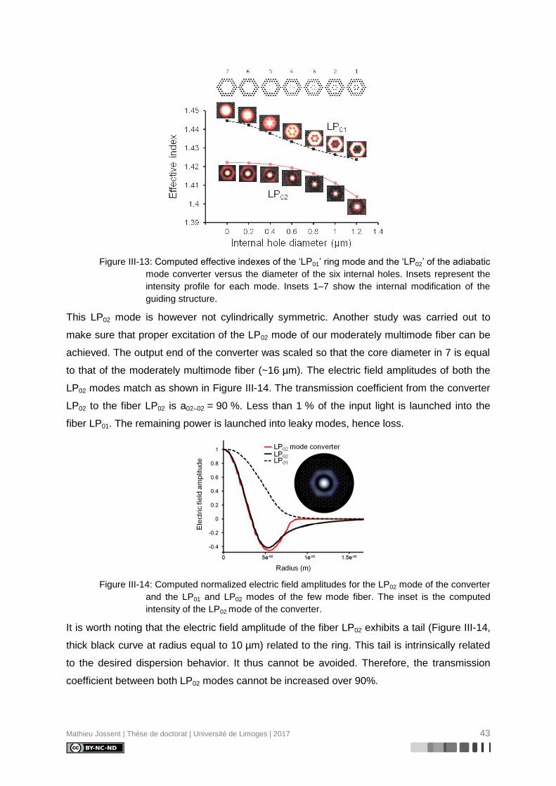
Mathieu Jossent | Thèse de doctorat | Université de Limoges | 2017 43
Figure III-13: Computed effective indexes of the ‘LP01’ ring mode and the ‘LP02’ of the adiabatic
mode converter versus the diameter of the six internal holes. Insets represent the
intensity profile for each mode. Insets 1–7 show the internal modification of the
guiding structure.
This LP02 mode is however not cylindrically symmetric. Another study was carried out to
make sure that proper excitation of the LP02 mode of our moderately multimode fiber can be
achieved. The output end of the converter was scaled so that the core diameter in 7 is equal
to that of the moderately multimode fiber (~16 µm). The electric field amplitudes of both the
LP02 modes match as shown in Figure III-14. The transmission coefficient from the converter
LP02 to the fiber LP02 is a02–02 = 90 %. Less than 1 % of the input light is launched into the
fiber LP01. The remaining power is launched into leaky modes, hence loss.
Figure III-14: Computed normalized electric field amplitudes for the LP02 mode of the converter
and the LP01 and LP02 modes of the few mode fiber. The inset is the computed
intensity of the LP02 mode of the converter.
It is worth noting that the electric field amplitude of the fiber LP02 exhibits a tail (Figure III-14,
thick black curve at radius equal to 10 µm) related to the ring. This tail is intrinsically related
to the desired dispersion behavior. It thus cannot be avoided. Therefore, the transmission
coefficient between both LP02 modes cannot be increased over 90%.
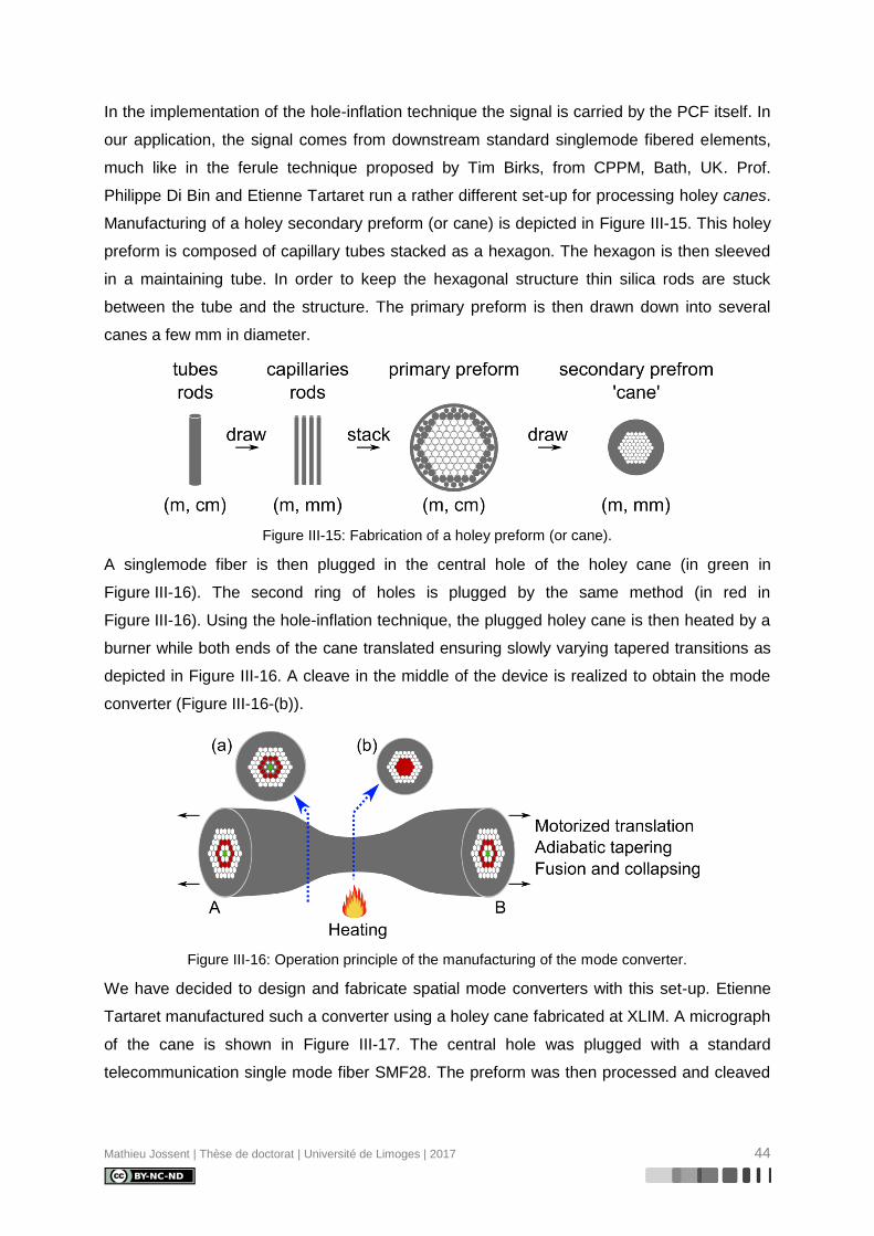
Mathieu Jossent | Thèse de doctorat | Université de Limoges | 2017 44
In the implementation of the hole-inflation technique the signal is carried by the PCF itself. In
our application, the signal comes from downstream standard singlemode fibered elements,
much like in the ferule technique proposed by Tim Birks, from CPPM, Bath, UK. Prof.
Philippe Di Bin and Etienne Tartaret run a rather different set-up for processing holey canes.
Manufacturing of a holey secondary preform (or cane) is depicted in Figure III-15. This holey
preform is composed of capillary tubes stacked as a hexagon. The hexagon is then sleeved
in a maintaining tube. In order to keep the hexagonal structure thin silica rods are stuck
between the tube and the structure. The primary preform is then drawn down into several
canes a few mm in diameter.
Figure III-15: Fabrication of a holey preform (or cane).
A singlemode fiber is then plugged in the central hole of the holey cane (in green in
Figure III-16). The second ring of holes is plugged by the same method (in red in
Figure III-16). Using the hole-inflation technique, the plugged holey cane is then heated by a
burner while both ends of the cane translated ensuring slowly varying tapered transitions as
depicted in Figure III-16. A cleave in the middle of the device is realized to obtain the mode
converter (Figure III-16-(b)).
Figure III-16: Operation principle of the manufacturing of the mode converter.
We have decided to design and fabricate spatial mode converters with this set-up. Etienne
Tartaret manufactured such a converter using a holey cane fabricated at XLIM. A micrograph
of the cane is shown in Figure III-17. The central hole was plugged with a standard
telecommunication single mode fiber SMF28. The preform was then processed and cleaved

Mathieu Jossent | Thèse de doctorat | Université de Limoges | 2017 45
so that the core region is approximately 17 µm in diameter as can be seen in Figure III-17-(b)
to fit the passive fiber core dimensions (Figure II-11-(a) blue).
(a) (b)
Figure III-17: (a) Micrograph of the holey cane used to manufacture the adiabatic converter. (b)
Micrograph of the output end facet of the manufactured converter.
III.3. Passive few mode fiber excited by the LP02 mode converter
The central fiber was then spliced to two ASE sources emitting on the erbium and thulium
band respectively. The near field intensity at the output of the converter was observed by
means of a thermal camera (Pyrocam). The observed near field intensities are shown in
Figure III-18. As we can see, the intensity patterns are shaped by the spatial light converter
and seem to be weakly wavelength dependent. In Figure III-18-(b), the camera gain was
increased in order to see the whole ring resulting in the saturation of the central lobe.
(a) (b)
Figure III-18: Near field output of the mode converter excited by (a) an Erbium ASE source
and (b) a Thulium ASE source.
A radial scan of the magnified and collimated near field was performed to gather another clue
on the weak wavelength dependence. At each point of this scan, the spectrum was collected.
Those measurements are summarized by Figure III-19.
17 µm

Mathieu Jossent | Thèse de doctorat | Université de Limoges | 2017 46
Figure III-19: Radial scan of the output near field of the mode converter excited by (a) the
Erbium ASE source with 41 points of measurements and (b) the Thulium ASE
source with 101 points of measurements. (c) and (d) are the respective radial
traces at the beginning and the end of both bandwidths.
The spectral evolution is rather constant over tens of nanometers in both bandwidths.
Furthermore, the intensity zeros are well defined in both bands. The weak wavelength
dependence over 300 nm of bandwidth is thus confirmed.
Then, a 20 m long piece of passive few mode fiber (which exhibits a core size really close to
that of the mode converter) was butt coupled to the mode converter end facet. The mode
converter was successively excited by both ASE sources as shown schematically in Figure
III-20.
Figure III-20: Experimental set-up to evaluate selective modal excitation of the passive few
mode fiber.
The field intensity at the output end of the passive few mode fiber is shown in Figure III-21.
The LP02 intensity pattern can be observed. The fiber was perturbed and coiled to check if

Mathieu Jossent | Thèse de doctorat | Université de Limoges | 2017 47
the guided mode would couple to any other mode of the fiber or if the excitation was realized
in both core and ring creating a virtual LP02 mode. No intensity changes were observed,
indicating weak coupling to other guided modes. The outer ring did not blink during this
process. If blinking would have been observed that would have meant that the excitation was
realized in both ring and core and that a ‘false’ LP02 was recorded.
(a) (b)
Figure III-21: Near field output of the passive few-mode fiber when excited by the mode
converter with (a) the Erbium ASE source and (b) the Thulium ASE source.
III.3.1. S² measurement on the passive few mode fiber excited by the mode converter
In order to quantitatively understand the behavior of this kind of mode converter I have
developed at XLIM the spatially- and spectrally-resolved imaging technique (S2) technique
proposed by Nicholson [33]. Explanations of the S2 as well as a description of the various
experiments carried out during my PhD are presented in Appendix 1. In the following, I will
only present the experimental results obtained with the association “mode converter-passive
FMF” using the Erbium and the Thulium ASE sources. Table III-2 shows the calculated
differential group delays normalized by the fiber length ( fibreg LcnfDGDs ) values for
all possible interferences in both bandwidths.
Table III-2: Calculated differential group delays normalized by the fiber length in (a) the Erbium
bandwidth and (b) the Thulium bandwidth. In both cases, the green cells show the
fDGDs involving the LP02 mode.
(a) (b)
fDGDs (ps/m)
LP11 LP21 LP02 LP31
LP01 5.18 10.78 10.46 86.36
LP11 5.60 5.27 10.67
LP21 0.32 5.08
LP02 5.40
fDGDs (ps/m)
LP11 LP21 LP02
LP01 6.19 11.52 4.47
LP11 5.33 1.73
LP21 7.05
In the Erbium band, the LP31 is guided but is close to its cut-off hence its high fDGD with the
LP01.
III.3.1.1. Erbium bandwidth
In this measurement, the spectral resolution of 1 pm allowed for a temporal window as wide
as 10 ps/m. If the LP01 and the LP02 produce an interference peak, temporal aliasing may

Mathieu Jossent | Thèse de doctorat | Université de Limoges | 2017 48
occur as the LP02-01 fDGDs is superior to the time window. This interference peak would thus
be seen at a delay of 0.46 ps/m. This peak may overlap with the LP02-21 interference peak
(0.32 ps/m) and produce a plateau. The recovered modes are presented in Figure III-22.
Figure III-22: S² measurement of the passive few-mode fiber excited by the mode converter on
the Erbium emission bandwidth for 20 m of fiber. 3 retrieved parasitic modes: LP21,
LP31 and LP11.
The LP01 was not retrieved in these measurements. This was attributed to the aliasing that
will nearly superimpose both the LP01 and LP21 interference peaks. However a plateau is not
observed hence the MPI of the LP01 must be lower than the noise floor (~-50 dB). The
measured MPIs and fDGDs are presented in Table III-3.
Table III-3: Measured differential group delays and multi-path interferences for the association
between the mode converter and the passive few mode fiber around 1.55 µm.
Measurement of LP21 LP31 LP11
fDGD (ps/m) 0.35 4.06 5.76
MPI (dB) -38 -42 -40
Very good agreement with the calculated fDGDs can be observed. Furthermore, the
excitation can be said pure since 99.97% of the total power is guided by the LP02.
III.3.1.2. Thulium bandwidth
Using the Thulium ASE source, the only retrieved parasitic mode is the LP11 with a slightly
higher MPI of -35 dB. The high temporal noise at short delays is attributed to the water
absorption peaks in this spectral window (see Appendix A.1.3). The recovered modes are
presented in Figure III-23.
-30
-25
-20
-15
-10
-5
0
0 2 4 6 8 10
Differential group delay (ps/m)
Su
m o
f sp
ectr
al
traces (
dB
)

Mathieu Jossent | Thèse de doctorat | Université de Limoges | 2017 49
Figure III-23: S² measurement of the passive few-mode fiber excited by the mode converter
within the Thulium emission bandwidth for 20 m of fiber. Only one retrieved
parasitic mode: LP11.
Both LP01 and LP21 were not retrieved in these measurements. This can be explained by
excitation proportions being lower than the noise floor (~-50 dB). The parasitic mode
measured characteristics are presented in Table III-4.
Table III-4: Measured differential group delays and multi-path interference values for the
association mode converter-passive few mode fiber in the Thulium bandwidth.
Measurement of LP11
fDGD (ps/m) 2.01
MPI (dB) -35
Very good agreement with the calculated fDGD is observed. Again, the excitation can be
said pure since 99.97% of power is contained in the LP02 mode.
These results constitute the first quantitative measurement of the excitation purity of a higher
order mode by a device different than a LPG.
III.4. SFSS from 1.6 to 2 um: pulsed seed source for similariton amplifier
Matching the input pulse central wavelength to Dmax allows reducing the impact of higher
order dispersion terms. Hence, a pulsed source able to achieve the spectral matching
between the pulse and the dispersion curve of the LP02 mode is highly desirable. I have
designed and fabricated a source of wavelength tunable ultrashort pulses covering the
spectral region from 1.6 to 2 µm. This source is based on the self-frequency shift process of
a soliton (see I.1.2) and its scheme is presented in Figure III-24. The pulse train is generated
by an all-fiber self-starting mode-lock laser generating 1 ps pulses with an average power of
0.7 mW at a wavelength of 1.56 µm with a FWHM of 4 nm. The pulses are stretched to avoid
any nonlinear amplification. At the output of the pre-amplifier, the pulses are a few ps in
duration with an average power of 10 mW. Then the pulses are directly amplified in a large
mode area Er-doped fiber amplifier. Finally a piece of singlemode passive fiber is used to
-35
-30
-25
-20
-15
-10
-5
0
0 1 2 3 4 5 6 7
Differential group delay (ps/m)
Su
m o
f sp
ectr
al
traces (
dB
)

Mathieu Jossent | Thèse de doctorat | Université de Limoges | 2017 50
shift the central wavelength further in the infrared. A high-pass filter with a cut-off wavelength
of 1.6 µm is placed after the output of the singlemode fiber.
Figure III-24: Setup scheme for the self-frequency shifted soliton source. Upper line is the
temporal shape along the setup with colors representing the pulse chirp (grey
stands for chirp equal to 0). Standard singlemode (SM) fibers are represented in
yellow, multimode (MM) fibers in dark yellow. HNLF highly nonlinear fiber, WDM
Wavelength Division Multiplexer, SM-EDF single mode erbium doped fiber, ErD-
DCF Erbium doped double-clad fiber, HP1.6 high-pass filter with 1.6 µm cut-off
wavelength.
By fine-tuning the high power pump diodes of the last stage of amplification, the energy
stored in the pulses is varied thus producing ejected solitons that will experience different
wavelength shift according to the input pump power. This dependence of the pulse central
wavelength on the pump power is shown in Figure III-25.
(a)
(b) (c) (d)
Figure III-25: (a) Measured evolution of the spectral profile at the output of the Raman
frequency-shifting fiber versus the pump power delivered to the last stage amplifier.
(b-d) Measured spectra at various pump power of 17, 19 and 23 W respectively
showing tunability from 1.8 to 1.99 µm.
(b) (c) (d)

Mathieu Jossent | Thèse de doctorat | Université de Limoges | 2017 51
The central wavelength of the output pulse can be swept from 1.8 to 1.99 µm to match Dmax
of the realized fibers. The pulse presents a spectral bandwidth ranging from 36 to 44 nm
FWHM with an average power ranging from 250 mW to 300 mW. As the output, the filtered
pulse is a fundamental soliton. It is Fourier-limited as shown in the auto-correlation trace in
Figure III-26 and presents a duration of 100 fs FWHM. These parameters will be used as
feeding parameters for the GNLSE solving software.
Figure III-26: Autocorrelation trace (blue) and hyperbolic secant squared fit (red circles) of the
output pulse centered at 1.9 µm wavelength. Inset is the full autocorrelation trace
showing the measuring range pedestal spanning from -100 to 100 ps.
III.5. Dispersion measurement
The dispersion of the LP02 mode has been measured using the setup in Figure III-27.
Figure III-27: Dispersion measurement setup using the SFSS source centered at 1.95 µm, the
dedicated mode converter and the passive few mode fiber
The soliton-shifted source was centered at 1.95 µm. The source output was fusion spliced to
the dedicated mode converter input. The mode converter output was successively
butt-coupled to 3 m and 1.5 m of the passive FMF. Measuring the auto-correlation trace and
the pulse spectrum at the output of the few-mode fiber in both configurations allowed
evaluating the dispersion around 1.95 µm. Figure III-28 shows the measurements of the
auto-correlation trace and spectrum in both cases. During the experiment, the spectral width
changed by 5 nm and the central wavelength drifted from 1.949 to 1.942 µm.
0
0.1
0.2
0.3
0.4
0.5
0.6
0.7
0.8
0.9
1
-2 -1.5 -1 -0.5 0 0.5 1 1.5 2
Time (ps)
No
rma
lize
d tra
ce
(a
.u.)
1.54 x 100 fs
Measure
Sech² fit

Mathieu Jossent | Thèse de doctorat | Université de Limoges | 2017 52
Figure III-28: Dispersion measurement with the SSFS source at 1.95 µm. (a) Autocorrelation
trace and (b) output spectrum for 1.5 m of passive few mode fiber excited by the
mode converter. (c) Autocorrelation trace and (d) out spectrum for 3 m.
The following equation was used to evaluate the dispersion:
(III.2)
with L the fiber length (1.5x10⁻³ km), t the FWHM duration difference (8.4 ps) and the
FWHM spectral bandwidth (ranging from 50 to 55 nm). The evaluated dispersion is
comprised between -102 and -112 ps/(nm.km) in very good agreement with the modeled
value of -108 ps/(nm.km). Side lobes can be observed in both autocorrelation traces.
However, contrary to what was observed by Morin [34] (in French), these ripples are not
consistent with other guided modes at this wavelength. This potentially comes from the
SSFS initial pulse centered at 1.56 µm which propagates in a totally different dispersion
regime.
Figure III-29: Dispersion measurement compared to expected value.
0
0.25
0.5
0.75
1
-200 -100 0 100 200
Time delay (ps)
Auto
corr
ela
tion
sig
nal (
a.u
.)
Measure
Sech² fit
1.54 x 4.6 ps
(a) (b)
55.125 nm
0
0.25
0.5
0.75
1
-400 -200 0 200 400
Time delay (ps)
Au
toco
rre
lation
sig
na
l (a
.u.)
Measure
Sech² fit
1.54 x 13 ps
(c)
0
0.1
0.2
0.3
0.4
0.5
0.6
0.7
0.8
0.9
1
1.85 1.9 1.95 2 2.05
Wavelength (µm)
Norm
aliz
ed
inte
nsity (a.u
.)
(d)
50 nm
L
tD
-150
-100
-50
0
50
1.85 1.9 1.95 2
Wavelength (µm)
Dis
pers
ion
(p
s/(
nm
.km
))
LP01
LP11
LP21
LP02
Measure

Mathieu Jossent | Thèse de doctorat | Université de Limoges | 2017 53
As can be seen in Figure III-29, the only mode presenting normal dispersion is the LP02.
Through this measurement, I confirmed a very good excitation by the mode converter of the
LP02 mode in a pulsed regime and the viability of this type of fiber to produce normal
dispersion in the short-wavelength infrared (SWIR). Moreover, this constitutes the first
measurement, to my knowledge, of the dispersion of a higher mode using an excitation
device other than a LPG.
III.6. Conclusion
In this chapter I have shown that the LP02 mode of a dispersion-tailored FMF can be
excited at two remote wavelengths of 1.55 and 2 µm by means of an adiabatic mode
converter. This device was designed and realized at XLIM using the hole-inflation technique.
The adiabatic mode converter allowed proper excitation of the LP02 with close to 100%
efficiency in the passive few-mode fiber as shown by the spectrally- and spatially-resolved
imaging technique. A tunable self-frequency shifted soliton source providing 100 fs pulses
with 250 mW average power from 1.6 to 2 µm was realized. The mode converter and the
tunable source were used to measure the chromatic dispersion of the LP02 mode around 1.95
µm. To my knowledge, this is the first report on a fiber providing high normal dispersion
(-108 ps/nm/km) at long wavelengths, far above the telecom window. Unfortunately, the
output facet of the mode converter was deteriorated during experiments. A new cleave was
performed without success preventing any satisfactory coupling into the few-mode fiber. Very
recently, Dr. Correa from CREOL provided us with photonic lanterns [35]–[38] that are being
tested. Nonetheless, these first experimental results show that, despite discrepancy between
the target RIP and the measured one, large normal dispersion and large effective area can
be achieved in the same fiber mode in the Tm-ion emission band near 2 µm. Armed with
these preliminary results I now describe the design, fabrication and characterization of an
active few-mode fiber.
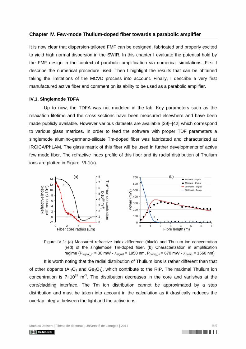
Mathieu Jossent | Thèse de doctorat | Université de Limoges | 2017 54
Chapter IV. Few-mode Thulium-doped fiber towards a parabolic amplifier
It is now clear that dispersion-tailored FMF can be designed, fabricated and properly excited
to yield high normal dispersion in the SWIR. In this chapter I evaluate the potential hold by
the FMF design in the context of parabolic amplification via numerical simulations. First I
describe the numerical procedure used. Then I highlight the results that can be obtained
taking the limitations of the MCVD process into account. Finally, I describe a very first
manufactured active fiber and comment on its ability to be used as a parabolic amplifier.
IV.1. Singlemode TDFA
Up to now, the TDFA was not modeled in the lab. Key parameters such as the
relaxation lifetime and the cross-sections have been measured elsewhere and have been
made publicly available. However various datasets are available [39]–[42] which correspond
to various glass matrices. In order to feed the software with proper TDF parameters a
singlemode alumino-germano-silicate Tm-doped fiber was fabricated and characterized at
IRCICA/PhLAM. The glass matrix of this fiber will be used in further developments of active
few mode fiber. The refractive index profile of this fiber and its radial distribution of Thulium
ions are plotted in Figure VI-1(a).
Figure IV-1: (a) Measured refractive index difference (black) and Thulium ion concentration
(red) of the singlemode Tm-doped fiber. (b) Characterization in amplification
regime (Psignal_in = 30 mW - signal = 1950 nm, Ppump_in = 670 mW - pump = 1560 nm)
It is worth noting that the radial distribution of Thulium ions is rather different than that
of other dopants (Al2O3 and Ge2O3), which contribute to the RIP. The maximal Thulium ion
concentration is 7×1025 m-3. The distribution decreases in the core and vanishes at the
core/cladding interface. The Tm ion distribution cannot be approximated by a step
distribution and must be taken into account in the calculation as it drastically reduces the
overlap integral between the light and the active ions.
0
1
2
3
4
5
6
7
8
-2
0
2
4
6
8
10
12
14
0 2 4 6
Fiber core radius (µm)
Re
fra
ctive
ind
ex
diffe
rence
(x1
0-3
)
Tm
3+-io
n c
on
ce
ntra
tion
(x1
02
5m
-3)
(a)
0
100
200
300
400
500
600
700
0 1 2 3 4 5 6 7
Fibre length (m)
Po
we
r (m
W)
Measure - Signal
Measure - Pump
3D Model - Signal
3D Model - Pump
(b)

Mathieu Jossent | Thèse de doctorat | Université de Limoges | 2017 55
TDFAs can be resonantly pumped in the telecom window at ~1.56 µm by EDFAs.
High-power TDFAs can also be pumped at 793 nm. The latter is useful providing the cross-
relaxation mechanism is efficient. This mechanism is efficient in highly-doped TDF, which is
not the case in the research fibers developed during this PhD. Therefore, the pump
wavelength lies around 1.56 µm and the pump radiation is supplied by a high-power cw
singlemode EDFA.
I have built a singlemode EDFA supplying 1.2 W of power at 1560 nm. This source is
based on a ring oscillator composed of two WDM (the first one protects the diode), a 70/30
output (30) coupler, 3 m of singlemode Er-doped fiber and an isolator. The ring laser is
pumped by a singlemode laser diode emitting 140 mW at 976 nm. This seed is then
amplified in an Er/Yb-doped DCF pumped using a 2+1:1 combiner by two multimode laser
diodes each emitting 6.5 W at 976 nm. The output of the amplifier was connected to an
isolator to avoid any back reflection. The schematic is presented in Figure IV-2.
Figure IV-2: Schematic of the high-power CW singlemode EDFA. ISO Isolator, 70/30 ring
output coupler with 30 being the output arm, 2+1:1 pump combiner and EYDCF
Erbium/Ytterbium doped double-clad fiber.
I have then characterized the fiber in amplification regime. The fiber was core-
pumped at 1560 nm. I have measured the output signal power as a function of the fiber
length and plotted the results in Figure VI-1(b) (black dots and triangles). The gain is low due
to the small amount of Tm-ions interacting with the light.
Then the TDFA was modeled taking into account the actual RIP and Tm-ion
distribution. Several datasets known from the literature for TDF, including the relaxation
lifetime and emission and absorption cross-sections, were implemented successively in the
software. Good quantitative agreement was obtained for a dataset provided in [41]. The
fluorescence lifetime is 560 µs. Emission and absorption cross-sections are plotted in
Figure IV-3. These values will be used in further developments of active few-mode fiber.

Mathieu Jossent | Thèse de doctorat | Université de Limoges | 2017 56
Figure IV-3: Tm3+
absorption (dashed-blue) and emission (red) cross-sections leading to a
good quantitative agreement between the measured and calculated evolutions of the pump
and signal powers along the fabricated fiber.
IV.2. Numerical procedure
The goal of this paragraph is to evaluate the potential hold by a Tm-doped version of
the fiber design shown in Figure IV-3 for parabolic amplification of ultrashort pulses in the
vicinity of 2 µm. The RIP and the expected Tm-ion concentration are schematically depicted
in Figure IV-3.
Figure IV-4: Refractive index profile (black) of a Tm3+
-doped few-mode fiber. α = 6,
n1 = 1510–3
, r1 = 8 µm, n2 = –410–3
, r2 = 4 µm, n3 = 310–3
, r3 = 8 µm. The
active ions distribution is flat in the core (red dotted). The Tm3+
concentration is
equal to 2.6x1025
m-3
(mean value of the SMF Tm3+
concentration).
Numerical modeling of a core-pumped few-mode TDFA has been carried out using an
in-house developed software according to the process depicted in Figure IV-3.
0
0.5
1
1.5
2
2.5
3
3.5
4
4.5
1.4 1.5 1.6 1.7 1.8 1.9 2 2.1 2.2
Wavelength (um)
Cro
ss s
ectio
n (x1
0-2
5m
2)
Emission
Absorption
0
0.5
1
1.5
2
2.5
3
-5
0
5
10
15
0 5 10 15 20 25 30
Fiber radius (um)
RIP
n (
x10
-3)
Tm
3+-io
n c
on
cen
tratio
n(x
10
25
m-3)

Mathieu Jossent | Thèse de doctorat | Université de Limoges | 2017 57
Figure IV-5: Numerical process based on three different in-house programs (red rectangles)
fed by the measured RIP and Thulium distribution (green circles) to obtain
several sets of data (blue arrows) resulting in the pulse spectral, temporal and
energetic evolution along its amplification in the core-pumped few-mode TDFA.
First, a mode solver for cylindrically symmetric fibers is fed by the refractive index
profile of the amplifying fiber shown in Figure IV-2. The mode solver gives every LPmn mode
(superscripts m and n correspond to azimuthal and radial indices) characterized by the
following parameters:
- effective index variations neffmn(),
- effective modal area variations Aeffmn()
- radial electrical field distribution variations Emn(r,).
Then, Emn(r,) is symmetrized according to the azimuthal number m to give Emn(r,,).
At the pump wavelength (C-band), the LP01, LP11, LP21, LP02 and LP31 modes are guided
(Figure IV-4). The LP31 cut-off wavelength is around 1.7 µm. In the Tm emission band, the
fiber will propagate the four lowest-order LP modes.
Figure IV-6: Guided LP modes of the few-mode TDF at = 1.56 µm.

Mathieu Jossent | Thèse de doctorat | Université de Limoges | 2017 58
Then, the rate equations for the multimode amplifier are solved by taking into account the
transverse distributions of electrical field for each co-propagated mode [43]. This software
gives the LP02 gain versus wavelength and longitudinal position G02(,z). This model takes
gain saturation into account. G02(,z) is of paramount importance to properly model gain
narrowing in ultrashort pulse amplifiers. It also accounts for the influence of ASE (carried by
any guided mode) and the effect of the shape of the pump in the core-pumping regime.
Finally, the GNLSE with gain (Eq I.11) is solved for in order to determine the spectral and
temporal properties of a pulse envelope carried by the LP02 mode in this amplifier. The
nonlinear program is fed by neff02(), G02(,z) and Aeff
02().
IV.2.1. Multimode amplification in continuous wave regime
A schematic of the numerical procedure for modeling multimode amplification in
continuous wave regime is shown in Figure II-14.
Figure IV-7: Modeling of a core-pumped multimode amplifier. The input powers of the pump
and signal are split among the guided modes at the respective wavelengths. The
output data give the new modal weights (and therefore modal power) at each
wavelength.
The population inversion N2(x,y,z) – N1(x,y,z) is discretized in all three spatial
coordinates with steps dx, dy and dz. The signal and pump input radiations are linear
combinations ofmn() Emn(x,y) where mn() is the modal weight at wavelength at the
input of the fiber. The rate equations are solved in each elementary section (dx×dy) in order
to evaluate the longitudinal variation of population inversion N2(x,y,z) – N1(x,y,z) and mn(z)
[43]. The signal and pump output radiations are then linear combinations ofmn(L) Emn(x,y).
Amplified spontaneous emission (ASE) is evenly distributed among the guided modes.
IV.2.1.1. Dependence of the gain on the pump wavelength
First I considered a singlemoded LP02 amplifier using the Optimal RIP for the modeled
fiber, both the pump and signal are carried by the LP02 mode. This core-pumped TDFA was
modeled to obtain the spectral and spatial dependence of the gain ( ,0P,zPG ) for

Mathieu Jossent | Thèse de doctorat | Université de Limoges | 2017 59
various pump wavelengths. The amplifier was seeded by a signal centered at Dmax
(1.907 µm) with a 40 nm bandwidth FWHM carrying 250 mW of power. The signal spectrum
is given a hyperbolic secant squared shape to model the high-repetition rate (48 MHz) pulsed
signal. The pump wavelength was varied from 1.535 µm, 1.550 µm, and 1.560 µm (C-band
EDFA) while the pump power was kept at 6 W. The spectral and spatial variation of the gain
is shown in Figure IV-6 for the three pump wavelengths. The contour line at value equal to
one represents transparency. The area below this line represents absorption.
Figure IV-8: Results from modeling of LP02 cw TDFA. Spectral and spatial evolution of the gain
for (a) p = 1.535 µm, (b) 1.55 µm, (c) 1.56 µm. Optimal lengths for maximal output
power are (a) 6.66 m, (b) 4.75 m, (c) 3.97 m, shown by dotted lines.
The TDFA must provide a gain bandwidth wide enough to amplify at least 50 nm of pulse
bandwidth so as to avoid pulse deterioration by e.g. gain filtering. Moreover the optimal
length (Lopt, where the amplified signal is maximized) must be as long as possible to take
advantage of the dispersion provided by the dispersion-tailored fiber. In the three cases, the
output signal power at Lopt is around 4.7 W. At short wavelengths, TDFA gain is lower than
one while at longer wavelength Lopt is too short to take advantage from the dispersion. Along
the amplification, at the pump wavelength of 1.535 µm, the pulse spectral FWHM increases
from 40 nm to 48 nm in the first two meters. Afterwards, the FWHM shrinks down to 37 nm at
Lopt and to 33 nm after 10 m of propagation as shown in Figure IV-9.
Figure IV-9: Spectral FWHM evolution along the amplification in the TDFA according to the
pump wavelength (a-blue) 1535 nm, (b-green) 1550 nm and (c-red) 1560 nm.
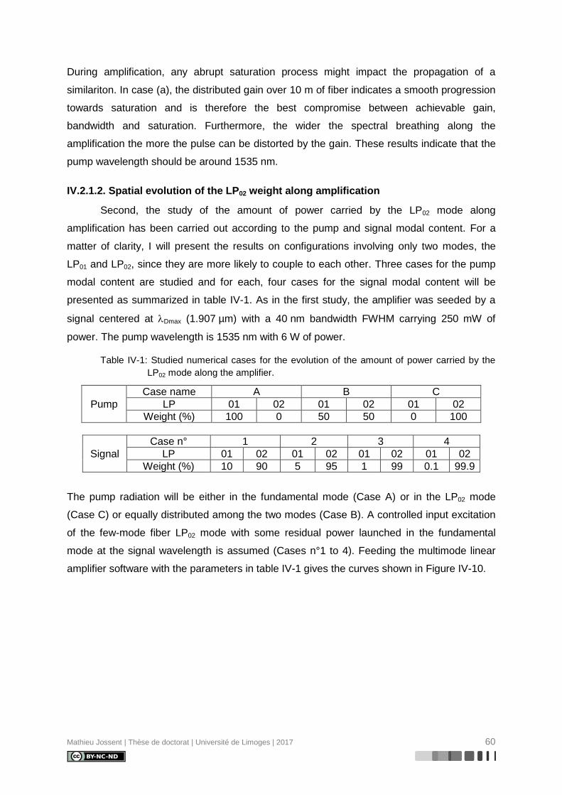
Mathieu Jossent | Thèse de doctorat | Université de Limoges | 2017 60
During amplification, any abrupt saturation process might impact the propagation of a
similariton. In case (a), the distributed gain over 10 m of fiber indicates a smooth progression
towards saturation and is therefore the best compromise between achievable gain,
bandwidth and saturation. Furthermore, the wider the spectral breathing along the
amplification the more the pulse can be distorted by the gain. These results indicate that the
pump wavelength should be around 1535 nm.
IV.2.1.2. Spatial evolution of the LP02 weight along amplification
Second, the study of the amount of power carried by the LP02 mode along
amplification has been carried out according to the pump and signal modal content. For a
matter of clarity, I will present the results on configurations involving only two modes, the
LP01 and LP02, since they are more likely to couple to each other. Three cases for the pump
modal content are studied and for each, four cases for the signal modal content will be
presented as summarized in table IV-1. As in the first study, the amplifier was seeded by a
signal centered at Dmax (1.907 µm) with a 40 nm bandwidth FWHM carrying 250 mW of
power. The pump wavelength is 1535 nm with 6 W of power.
Table IV-1: Studied numerical cases for the evolution of the amount of power carried by the
LP02 mode along the amplifier.
Pump
Case name A B C
LP 01 02 01 02 01 02
Weight (%) 100 0 50 50 0 100
Signal
Case n° 1 2 3 4
LP 01 02 01 02 01 02 01 02
Weight (%) 10 90 5 95 1 99 0.1 99.9
The pump radiation will be either in the fundamental mode (Case A) or in the LP02 mode
(Case C) or equally distributed among the two modes (Case B). A controlled input excitation
of the few-mode fiber LP02 mode with some residual power launched in the fundamental
mode at the signal wavelength is assumed (Cases n°1 to 4). Feeding the multimode linear
amplifier software with the parameters in table IV-1 gives the curves shown in Figure IV-10.

Mathieu Jossent | Thèse de doctorat | Université de Limoges | 2017 61
Figure IV-10: LP02 weight evolution along amplification in (a) case A, (b) case B and (c) case
C. Black dotted circles are the respective Lopt where the amount of power in the
LP02 mode is the highest.
From these results, two observations can be made. First, in every case, the weight of the
LP02 mode is decreasing along the amplifier. However, the strongest modal degradation is
observed in case A (Figure IV-10-(a)). This can be explained by the fact that the Tm ions are
pumped in the fundamental mode only, thus the inverted population maps the LP01 mode
intensity. Therefore, the modal content at the amplifier output changes dramatically due to an
enhanced amplification of the portion of the signal launched in the LP01 mode. Second, Lopt is
decreased from 6.66 m to less than 4 m when compared to what was expected by the gain
spectral and spatial dependences explained in the previous point. This can be explained by
the modal competition occurring during amplification. Lopt is calculated when the amount of
power in the LP02 is the highest however along the amplification the weight of the LP02 mode
decreases thus the balance between those two parameters produce a lower Lopt. It can be
noticed that the higher the LP02 weight the longer Lopt (Case C1-4 in Figure IV-10-(c)). The
different power carried by the LP02 at each Lopt is summarized in table IV-2. The highest
power is obtained for the case C4 where the pump is fully carried by the LP02 and the input
signal has the highest weight of LP02.
Table IV-2: Calculated Lopt and power carried by the LP02 mode at Lopt in every case
combination.
Case A B C
N° 1 2 3 4 1 2 3 4 1 2 3 4
Lopt (m) 2.11 2.25 2.62 3.26 2.28 2.42 2.82 3.43 2.58 2.78 3.27 3.8
P02(Lopt) (W) 1.7 2.2 3.2 4.1 2.13 2.64 3.6 4.4 2.88 3.44 4.26 4.64
The amount of power that is not carried by the LP02 mode will be useless in the similariton
amplifier. It is thus compulsory to have the highest weight of LP02 at both pump and signal
wavelengths to take full advantage of both the dispersion and the amplifier.
(a)
253035404550556065707580859095
100
0 1 2 3 4 5 6 7 8 9 10
Fiber length (m)
LP
02
we
igh
t (%
) 1D
1C
1B
1A
A4
A3
A2
A1
LP
02
weig
ht
(%)
(b)
253035404550556065707580859095
100
0 1 2 3 4 5 6 7 8 9 10
Fiber length (m)
LP
02
we
igh
t (%
)
2D
2C
2B
2A
B4
B3
B2
B1
LP
02
weig
ht
(%)
(c)
253035404550556065707580859095
100
0 1 2 3 4 5 6 7 8 9 10
Fiber length (m)
LP
02
we
igh
t (%
)
3D
3C
3B
3A
C4
C3
C2
C1LP
02
weig
ht
(%)

Mathieu Jossent | Thèse de doctorat | Université de Limoges | 2017 62
IV.2.1.3. Enhanced design
A way to release the constraint on the modal conversion at the pump wavelength has been
explored. This solution relies on the delocalization of the fundamental from the active media
by modifying the RIP. Using the knowledge gathered in Chapter II, the enhanced profile
presented in the Figure IV-11-(a) has been tuned so that its LP02 will produce roughly the
same amount of dispersion as the optimal profile but centered at Dmax = 1.85 µm (Figure
IV-11-(b)). At this wavelength, the LP02 mode presents an effective area of 440 µm². The
opto-geometrical parameters are summarized in table IV-3.
Table IV-3: Opto-geometrical parameters of the enhanced few-mode fiber and LP02
characteristics at Dmax.
Enhanced RIP
n r
Depressed active core 810–3 3
Core 1610–3 9
Trench –410–3 4
Ring 310–3 9.5
D02(Dmax) [ps/(nm.km)] -350
Aeff02(Dmax) [µm²] 440
FOM [fs] 136
The Dmax was shorten allowing a balanced amplification of the pulse spectral components.
This is due to two phenomena opposing each other. On one hand, as the mode is generating
dispersion, its overlap integral with the gain media is decreasing (Figure IV-11-(c)) hence
unbalancing the spectral amplification in favor of the short wavelengths. On the other hand,
the longer the amplifier, the higher the gain at longer wavelengths. When taking into account
both phenomena, we can expect a balanced amplification of the pulse at the fiber output.
Figure IV-11: (a) Enhanced RIP and Tm3+
modeled distribution. (b) Calculated dispersion
curve of the LP02 mode in this design. (c) Overlap integral for each mode.
The same study concerning the spatial evolution of the LP02 weight along the amplifier has
been carried out giving the curves in Figure IV-12. As can be seen, not only is the signal
0
0.5
1
1.5
2
2.5
3
-5
0
5
10
15
0 5 10 15 20 25 30
Fiber radius (um)
RIP
n
(x1
0-3
)
Tm
3+-io
n c
on
ce
ntra
tion
(x1
02
5m
-3)
(a)
-350
-300
-250
-200
-150
-100
-50
0
50
1.6 1.65 1.7 1.75 1.8 1.85 1.9 1.95
Dis
pe
rsio
n (p
s/(
nm
.km
))
Wavelength (µm)(b)
0
5
10
15
20
25
30
35
40
1.6 1.65 1.7 1.75 1.8 1.85 1.9 1.95
Wavelength (um)
Overl
ap
inte
gra
lw
ith
ga
in m
ed
ia (
%)
(c)
LP02
LP01
LP11
LP21
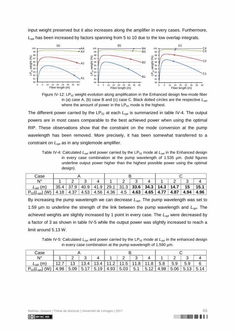
Mathieu Jossent | Thèse de doctorat | Université de Limoges | 2017 63
input weight preserved but it also increases along the amplifier in every cases. Furthermore,
Lopt has been increased by factors spanning from 5 to 10 due to the low overlap integrals.
Figure IV-12: LP02 weight evolution along amplification in the Enhanced design few-mode fiber
in (a) case A, (b) case B and (c) case C. Black dotted circles are the respective Lopt
where the amount of power in the LP02 mode is the highest.
The different power carried by the LP02 at each Lopt is summarized in table IV-4. The output
powers are in most cases comparable to the best achieved power when using the optimal
RIP. These observations show that the constraint on the mode conversion at the pump
wavelength has been removed. More precisely, it has been somewhat transferred to a
constraint on Lopt as in any singlemode amplifier.
Table IV-4: Calculated Lopt and power carried by the LP02 mode at Lopt in the Enhanced design
in every case combination at the pump wavelength of 1.535 µm. (bold figures
underline output power higher than the highest possible power using the optimal
design).
Case A B C
N° 1 2 3 4 1 2 3 4 1 2 3 4
Lopt (m) 35.4 37.9 40.9 41.9 29.1 31.3 33.6 34.3 14.3 14.7 15 15.1
P02(Lopt) (W) 4.18 4.37 4.53 4.56 4.36 4.5 4.63 4.65 4.77 4.87 4.94 4.96
By increasing the pump wavelength we can decrease Lopt. The pump wavelength was set to
1.59 µm to underline the strength of the link between the pump wavelength and Lopt. The
achieved weights are slightly increased by 1 point in every case. The Lopt were decreased by
a factor of 3 as shown in table IV-5 while the output power was slightly increased to reach a
limit around 5.13 W.
Table IV-5: Calculated Lopt and power carried by the LP02 mode at Lopt in the enhanced design
in every case combination at the pump wavelength of 1.590 µm.
Case A B C
N° 1 2 3 4 1 2 3 4 1 2 3 4
Lopt (m) 12.7 13 13.4 13.4 11.2 11.5 11.8 11.8 5.8 5.9 5.9 6
P02(Lopt) (W) 4.98 5.09 5.17 5.19 4.93 5.03 5.1 5.12 4.98 5.06 5.13 5.14
90
91
92
93
94
95
96
97
98
99
100
0 5 10 15 20 25 30 35 40
Fiber length (m)
LP
02
we
igh
t (%
)
A4A3
A2
A1
(a)
90
91
92
93
94
95
96
97
98
99
100
0 5 10 15 20 25 30 35 40
Fiber length (m)L
P0
2w
eig
ht
(%)
B4B3
B2
B1
(b)
90
91
92
93
94
95
96
97
98
99
100
0 5 10 15 20 25 30 35 40
Fiber length (m)
LP
02
we
igh
t (%
)
C4C3
C2
C1
(c)

Mathieu Jossent | Thèse de doctorat | Université de Limoges | 2017 64
Figure IV-13: Results from modeling of LP02 cw TDFA in the enhanced few-mode fiber design.
Spectral and spatial evolution of the gain for case (a) A4 (b) B4 (c) C4. Optimal
lengths for maximal output power are shown by dotted lines.
From these results, we can say that the enhanced design transferred the pump modal
conversion constraint to a kind of Lopt constraint. As can be seen in table IV-5, converting the
pump mode to the LP02 will decrease the required amplifier length by 2 all other things being
equal. This decrease in length will produce strong variations of the gain in short pieces of
fiber. As we wanted to avoid these fluctuations it would even be better to carry the pump on
the fundamental mode of this fiber as confirmed by the spectral gain evolutions along the
fiber presented in Figure IV-13. A preform of this fiber is currently being realized at
IRCICA/PhLAM.
IV.2.2. Nonlinear modeling
Here will be presented the different calculations realized on the optimal profile. I have
focused my study on the evolution of the spectral and temporal properties of a pulse carried
only by the LP02 mode during its propagation in a dispersion-tailored active few-mode fiber.
Equation I.31
eff
32
2
AD
gn8
cΕ̂
gives the maximum extractable energy before wavebreaking. Applying this equation to the
computed optimal RIP with the same parameters as in I.2.3.1 (g = 1.9 Np/m and full =
105 nm) we obtain the results summarized in table IV-6.
IV-6: Calculated maximum extractable energy of an amplified similariton in the optimal design.
Fiber Optimal
Dmax (µm) 1.908
|Dmax| (ps/(nm.km)) -380
Aeff (µm²) 353
Ê (µJ) 27

Mathieu Jossent | Thèse de doctorat | Université de Limoges | 2017 65
The energy of a similariton propagating in the LP02 mode in this fiber can reach 27 µJ
before wavebreaking. This equation, relies on several approximations: the gain is constant
along the fiber; the dispersion and effective area are not wavelength-dependent. In order to
understand whether this equation is valid in more realistic conditions, I have modeled the
propagation of an ultrashort pulse in the optimal fiber design by solving the GNLSE. I have
assumed a constant gain of 1.9 Np/m, a constant effective area of 353 µm² while wavelength
dependence of D was included. Two seed pulses were tested, an unrealistic 1 ps pulse and
a realistic 100 fs to study the equation I.31 and the influence of effective area and gain
dependence to wavelength.
IV.2.2.1. Constant effective modal area and gain
This study is focused on the evaluation of similariton wavebreaking. A similariton
wavebreaking can be identified in two ways. First, the temporal or spectral shape is no more
a parabola hence the pulse is no more a similariton. Second, the chirp has to be linear, if the
chirp is no more linear we cannot define the pulse as a similariton.
IV.2.2.1.1. Unrealistic 1 ps pulse
The seed pulse in this numerical simulation is an unchirped soliton with the characteristics
reported in table IV-7.
Table IV-7: Input pulse temporal and spectral characteristics.
Pulse characteristic Value
t (ps) 1
(nm) 4
Ê (nJ) 10
Chirp 0
Its temporal and spectral shapes are represented in Figure IV-14. This pulse was deliberately
set to unrealistic values since the purpose of this simulation was to quickly reach
wavebreaking to compare the model and what was expected by Equation I.31.

Mathieu Jossent | Thèse de doctorat | Université de Limoges | 2017 66
Figure IV-14: Numerical simulations of the input (a) temporal (t = 1 ps) and (b-black) spectral
profile ( = 4 nm) of the pulse carrying 10 nJ of energy seeding the core-doped
optimal few-mode fiber with constant gain (1.9 Np/m), assuming constant effective
area of 353 µm² and wavelength dependent dispersion (b-red).
The temporal and spectral shapes at the fiber output are presented in Figure IV-15-(a-b). The
soliton launched into the fiber amplifier shapes, in the temporal domain, towards a parabola
after few centimeters of propagation in the fiber. Then, the parabolic temporal shape is
maintained and enlarged along amplification as can be expected from a similariton.
Figure IV-15-(a) shows the strong temporal breathing along the amplifier from 1 ps to 40 ps.
In the same time, the pulse spectrum also broadens due to nonlinear Kerr effect. The pulse
energy grows exponentially from 10 nJ to 20 µJ without wavebreaking.
The pulse temporal profile is slightly distorted, though, due to higher-order dispersion
parameters (3, 4,…) included in the simulation.
Figure IV-15: Numerical simulations showing the longitudinal evolution of (a) temporal and (b)
spectral profiles of a pulse propagating in the optimal few-mode fiber, assuming
constant effective area of 353 µm² and wavelength dependent dispersion. The
profiles are normalized to 1 at each position. (c) Evolution of the pulse energy
along the amplifier (constant gain of 1.9 Np/m).
The wavebreaking can be identified by looking at the pulse envelope and the chirp. On one
hand, if the envelope has located features, then wavebreaking is starting as shown by Figure
IV-16-(b-c).

Mathieu Jossent | Thèse de doctorat | Université de Limoges | 2017 67
Figure IV-16: Numerical simulations showing evolution of the temporal (first row) and
normalized spectral (second row) profiles of the pulse for various fiber lengths: (a-
e) 4 m, (b-f) 4.19 m, (c-g) 4.23 m and (d-e) 4.25m.
In Figure IV-16-(b), wavebreaking is starting, the pulse temporal shape starts to locally
oscillate due to nonlinear process occurring at both zeros of the modeled dispersion of the
LP02 mode (1.73 µm and 2.08 µm). After few centimeters, the pulse will present stronger
oscillations as shown in Figure IV-16-(c-d) due to the constant gain. At longer pieces of fiber,
every wavelength will experience the constant gain and nonlinear effects will occur and
overwhelm the pulse. Nonetheless, the energy comprised in the pulses presented in the first
row of Figure IV-14 is above 20 µJ as shown in Table IV-8.
Table IV-8: Numerical simulations showing the achieved energy in the active optimal few-
mode fiber with constant gain of 1.9 Np/m, constant Aeff of 353 µm² and wavelength
dependent dispersion.
Figure label Fiber length (m) Energy (µJ)
a 4 20.2
b 4.19 28.7
c 4.23 30.7
d 4.25 32.15
The wavelengths at the zeros of dispersion exceed the -100 dB threshold at 23.8 µJ of
energy at the fiber length of 4.1 m. Afterwards, temporal features are noticeable. The
generation of wavelength on or near the zeros of dispersion is the limitation to the energy
scaling of a similariton.
A lossless double-passing compression line was modeled to check the compressibility of the
amplified pulse. This compression line only compensates for the two first orders of dispersion
(1 and 2). This line is composed of two transmission gratings with a resolution of
560 lines/mm (PCG-560-2000-933 from Ibsen photonics) placed at the Littrow angle (34°).
For a distance between the two gratings of 5.37 cm, the pulse in Figure IV-16-(a) is
compressed down to 180 fs FWHM (Figure IV-17). The compressed pulse presents

Mathieu Jossent | Thèse de doctorat | Université de Limoges | 2017 68
unbalanced side bands due to higher order dispersion not compensated for by the gratings.
This results in having 55% of the pulse energy contained in the 180 fs central peak allowing
reaching 61.8 MW peak power.
Figure IV-17: Numerical simulations showing the compression of the output pulse (z = 4 m)
down to 180 fs FWHMI by a grating compressor in the case of the unrealistic input
pulse (10 nJ, 1 ps, 4 nm).
These results are presented to underline the possibilities of similariton amplifiers when
considering a constant distributed gain (1.9 Np/m) and effective area (353 µm²). The pulse,
carried by a purely excited highly dispersive LP02, can be recompressed to 180 fs pulse
duration with over 10 µJ energy in its central lobe.
IV.2.2.1.2. Realistic 100 fs pulse
However, with an input pulse with a broader spectrum as is the case for fs pulse, SPM could
be triggered closer to the dispersion zeros limiting the stored energy before wavebreaking.
Notwithstanding, the spectral power density is drastically lowered compared to ps pulses,
thus the SPM process that will impose the wavebreaking should be reached later in the fiber
when compared to the unrealistic ps pulse. To underline this assumption a realistic fs pulse
was used all other things being equal. Table IV-9 summarizes the realistic pulse
characteristics.
Table IV-9: Input pulse temporal and spectral realistic characteristics taken from the SFSS
source.
Pulse characteristic Value
t (fs) 100
(nm) 40.5
Ê (nJ) 5.2
Rep_rate (MHz) 48
Average power (mW) 250
Chirp 0
Figure IV-18 shows the temporal and spectral profile of this pulse; plus the dispersion and
the effective area evolutions according to wavelength.
180 fs

Mathieu Jossent | Thèse de doctorat | Université de Limoges | 2017 69
Figure IV-18: (a) temporal and (b-c) spectral profiles of the realistic seed pulse. In (b) the red
curve shows the dispersion. In (c) the red curve shows the effective area.
Figure IV-19 presents the normalized temporal and spectral shape evolution in the fiber
amplifier when seeded with the realistic pulse and the energy evolution along the amplifier. It
can be noticed that after 4 m of fiber, the spectral shapes is widening due to SPM process.
The effect on the pulse temporal and spectral shapes is in no way comparable to the
unrealistic pulse behavior. Nevertheless, the temporal shape is still an homothetic
transformation (Figure IV-20-(a-c)) whereas this is not the case for the spectral shape
(Figure IV-20-c). The chirp departs from the linear case as shown in Figure IV-20-(d).
Figure IV-19: Numerical simulations showing the normalized temporal (a) and spectral (b)
shape of the pulse along the fiber amplifier. (c) is the energy evolution along the
fiber (dotted blue line shows the energy at 4 m and dashed red line at 4.5 m). The
input pulse is the realistic pulse from the SFSS source.
0
200
400
600
800
1000
1200
1400
0
0.2
0.4
0.6
0.8
1
1.80 1.85 1.90 1.95 2.00Wavelength [um]
No
rma
lize
din
ten
sity
Eff
ective a
rea
[u
m²]
(c)

Mathieu Jossent | Thèse de doctorat | Université de Limoges | 2017 70
Figure IV-20: Numerical simulations showing (a) the temporal shape and chirp of the pulse
after 4 m of fiber. (b) the normalized pulse spectra after 4 and 4.5 m of fiber. (c) the
temporal shape and chirp of the pulse after 4.5 m of fiber. (d) The chirp parameter
of the pulse after 4 and 4.5 m of fiber. The input pulse is the realistic pulse from the
SFSS source.
The maximum energy contained in the pulse while keeping a linear chirp (after 4 m of fiber)
is 10.2 µJ. The pulse can be recompressed from 39 ps FWHM to 183 fs by the same gratings
compressor line with a distance of 5.6 cm (Figure IV-21). The fraction of energy in the central
recompressed lobe is 43% leading to 23.9 MW peak power.
Figure IV-21: Numerical simulations showing the compression of the output pulse (z = 4 m)
down to 183 fs FWHMI by a grating compressor in the case of the realistic input
pulse (5.2 nJ, 100 fs, 40 nm).

Mathieu Jossent | Thèse de doctorat | Université de Limoges | 2017 71
IV.2.2.2. Effective modal area
For the LP02 mode, the dispersion variation arises from a variation in radial electric
field distribution, hence it is accompanied with a large variation of the effective area. The
wavelength dependence of the effective area is also likely limiting factor that must be taken
into account in the modeling. For example, the variation of effective area of the LP02 mode
versus wavelength is plotted in Figure IV-22. It varies from 149 to 899 µm² between 1.85 and
1.95 µm. This variation directly impacts the calculated value of . The impact of the effective
area wavelength dependence is stronger when using the unrealistic pulse since the spectral
shape is generated via SPM.
Figure IV-22: Calculated LP02 effective area according to wavelength in the optimal fiber.
Dotted circle is Aeff02
(Dmax) = 353 µm².
IV.2.2.2.1. Unrealistic 1 ps pulse
During the amplification of the unrealistic 1 ps pulse, the nonlinearities are prone to happen
at the blue edge of the pulse due to a lower effective area. Thus, the generation of new
frequencies via SPM is no more balanced. This results in producing a ‘wall-effect’ on the red
edge of the pulse, as shown in Figure IV-23-(b), which is directly related to the steep slope of
with wavelength. This results in stopping the spectral, and thus the temporal, broadening.
Figure IV-23: Numerical simulations showing (a) temporal and (b) spectral profile of the
unrealistic pulse propagating in the optimal few-mode fiber with wavelength-
dependent dispersion and effective area. Gain is constant (1.9 Np/m). (c) Evolution
of the pulse energy along the amplifier.
0
200
400
600
800
1000
1200
1400
1.55 1.65 1.75 1.85 1.95 2.05
Wavelength (um)
LP
02
eff
ective
are
a (
um
2)
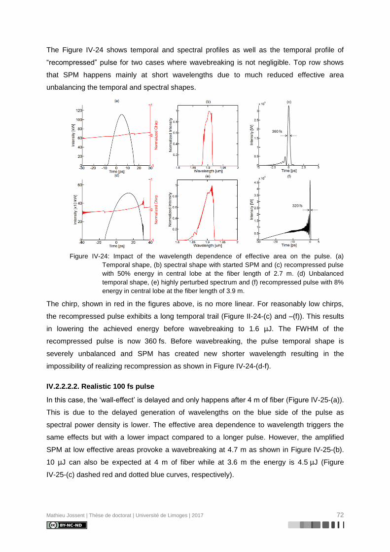
Mathieu Jossent | Thèse de doctorat | Université de Limoges | 2017 72
The Figure IV-24 shows temporal and spectral profiles as well as the temporal profile of
“recompressed” pulse for two cases where wavebreaking is not negligible. Top row shows
that SPM happens mainly at short wavelengths due to much reduced effective area
unbalancing the temporal and spectral shapes.
Figure IV-24: Impact of the wavelength dependence of effective area on the pulse. (a)
Temporal shape, (b) spectral shape with started SPM and (c) recompressed pulse
with 50% energy in central lobe at the fiber length of 2.7 m. (d) Unbalanced
temporal shape, (e) highly perturbed spectrum and (f) recompressed pulse with 8%
energy in central lobe at the fiber length of 3.9 m.
The chirp, shown in red in the figures above, is no more linear. For reasonably low chirps,
the recompressed pulse exhibits a long temporal trail (Figure II-24-(c) and –(f)). This results
in lowering the achieved energy before wavebreaking to 1.6 µJ. The FWHM of the
recompressed pulse is now 360 fs. Before wavebreaking, the pulse temporal shape is
severely unbalanced and SPM has created new shorter wavelength resulting in the
impossibility of realizing recompression as shown in Figure IV-24-(d-f).
IV.2.2.2.2. Realistic 100 fs pulse
In this case, the ‘wall-effect’ is delayed and only happens after 4 m of fiber (Figure IV-25-(a)).
This is due to the delayed generation of wavelengths on the blue side of the pulse as
spectral power density is lower. The effective area dependence to wavelength triggers the
same effects but with a lower impact compared to a longer pulse. However, the amplified
SPM at low effective areas provoke a wavebreaking at 4.7 m as shown in Figure IV-25-(b).
10 µJ can also be expected at 4 m of fiber while at 3.6 m the energy is 4.5 µJ (Figure
IV-25-(c) dashed red and dotted blue curves, respectively).
360 fs
320 fs

Mathieu Jossent | Thèse de doctorat | Université de Limoges | 2017 73
Figure IV-25: Numerical simulations showing (a) temporal and (b) spectral profile of the
realistic pulse propagating in the optimal few-mode fiber with wavelength-
dependent dispersion and effective area. Gain is constant (1.9 Np/m). (c) Evolution
of the pulse energy along the amplifier (dotted blue line shows the energy at 3.6 m
and dashed red line at 4 m)
However, the effect of the effective area on the pulse spectrum can be seen as early as at
4 m of fiber. As the pulse experience different parameters along its spectrum it provokes an
unbalance in the spectral growth (Figure IV-26-(b)). This disequilibrium has a direct impact
on the pulse chirp (Figure IV-26-(d)) and thus prevent good recompression with the modeled
gratings as shown with the unrealistic pulse. The pulse presented in Figure IV-26-(a) can be
recompressed from 34 ps FWHM to 183 fs with a grating distance of 5.15 cm (Figure IV-27).
The energy fraction contained in the central lobe is 46% leading to 11 MW peak power.
Figure IV-26: Numerical simulations showing (a) the temporal shape and chirp of the pulse
after 3.6 m of fiber. (b) the normalized pulse spectra after 3.6 and 4 m of fiber. (c)
the temporal shape and chirp of the pulse after 4 m of fiber. (d) The chirp

Mathieu Jossent | Thèse de doctorat | Université de Limoges | 2017 74
parameter of the pulse after 3.6 and 4 m of fiber. The input pulse is the realistic
pulse from the SFSS source.
The effective area wavelength dependence is a first limitation to the energy scaling of a
similariton. The maximum reachable energy without any deformation is scaled by a factor 6
going from 27 to 4.5 µJ when including the effective area variation in the GNLSE.
Nevertheless, the microjoule milestone is still in the scope when considering a constant gain
over every wavelength. Moreover, the realistic pulse gives better results when the effective
area wavelength dependence is considered. Therefore, only the realistic pulse will be studied
in the following.
Figure IV-27: Numerical simulations showing the compression of the output pulse (z = 4 m)
down to 183 fs FWHMI by a grating compressor in the case of the realistic input
pulse (5.2 nJ, 100 fs, 40 nm).
IV.2.2.3. Gain
The gain dependence to wavelength and fiber length is modeled by feeding the GNLSE with
the results of the linear amplification model (Figure II-16-(a)). The effective area is kept
constant and equal to 353 µm². In the spectral domain, the shorter wavelengths generated by
SPM will experience gain in the first meter of fiber. The blue wing of the pulse will then be
gradually reabsorbed, preventing any large spectral broadening via nonlinear effects at short
wavelength. This explains the pulse recall observed on the time and spectral domain
presented in Figure IV-28-(a-b). The energy is now limited to 99 nJ at Lopt equal to 8.78 m
due to the gain longitudinal and spectral influence. The pulse shape at Lopt is a similariton as
shown in figure IV-29-(a-b). The pulse is however delayed of 25 ps due to the back and forth
imposed by the SPM combined to available gain at short wavelength along the amplification.
During this back and forth, the pulse experience a lot of different high order dispersion values
along its spectrum that cannot be recompressed by the compressor line. Nevertheless, for a
grating distance of 18.4 cm, the pulse can be recompressed from 66.5 ps to 192 fs with a
central lobe containing 63% of the total energy. This leads to a 325 kW peak power.

Mathieu Jossent | Thèse de doctorat | Université de Limoges | 2017 75
Figure IV-28: Numerical simulations showing (a) temporal and (b) spectral profile of the
realistic pulse propagating in the optimal few-mode fiber with wavelength-
dependent dispersion and gain. Effective area is constant (353 µm²). (c) Evolution
of the pulse energy along the amplifier (dashed red line shows the energy at Lopt)
Figure IV-29: Numerical simulations showing (a) temporal and (b) spectral profile of the pulse
at Lopt in the optimal few-mode fiber with wavelength-dependent dispersion and
gain. Effective area is constant (353 µm²). (c) Recompressed pulse with 192 fs
duration.
The inclusion of the gain spectral and longitudinal dependence drastically reduces the
energy that can be aimed for lowering the value from over 4 µJ to 100 nJ.
IV.2.2.4. Effective area and gain
Both effective area and gain dependence to wavelength were then implemented in the
GNLSE giving the pulse normalized temporal and spectral evolutions along the fiber shown
in Figure IV-30-(a-b). The inclusion the effective are dependence to wavelength reduces the
Lopt to 7 m. This can be explained by the enhanced SPM produced at the blue side of the
pulse being amplified at the beginning of the fiber. These wavelengths will have stored more
energy compared to the constant effective area case. A balance in total energy between the
re-absorption of these wavelengths and the amplification of the red part of the pulse is
established. The highest value of energy can therefore be reached at shorter pieces of fiber
but with a spectrum centered at a shorter wavelength compared to the constant effective
area case. This is confirmed by the spectral shape of the pulse at Lopt shown in
Figure IV-31-(b). The energy at Lopt is 100 nJ which is close to what we had obtained with a

Mathieu Jossent | Thèse de doctorat | Université de Limoges | 2017 76
constant effective area. No other change in the pulse behavior can be noticed from the
inclusion of the effective area variation according to wavelength.
Figure IV-30: Numerical simulations showing (a) temporal and (b) spectral profiles of the
realistic pulse propagating in the optimal few-mode fiber with
wavelength-dependent dispersion, effective area and gain. (c) Evolution of the
Energy along the fiber amplifier (dashed red line is the energy at Lopt).
In Figure IV-31 are shown the temporal and spectrum intensities at Lopt and the
recompressed pulse. The temporal broadening of the pulse is asymetric due to lower
wavelengths being generated and amplified leading to a pulse FWHM of 58.4 ps with a
18.7 ps delay. SPM does not occur at longer wavelengths due to the large effective area,
one order of magnitude larger than that at shorter wavelengths as well as low distributed
gain. The spectral broadening is thus limited by the gain and the absorption at shorter
wavelengths and by the large effective area at longer wavelengths. Moreover, the shorter
wavelengths will experience different higher order dispersions (sign of beta4) compared to
the longer wavelengths. This delays the pulse and makes it asymmetric. Due to those limiting
effects, the output energy is reduced to 100 nJ. However, the output pulse can still be
recompressed down to 192 fs. The central peak contains 52% of the total energy leading to
272 kW peak power.
Figure IV-31: Numerical simulations showing (a) temporal and (b) spectral profiles of the
realistic pulse at Lopt in the optimal few-mode fiber with wavelength-dependent
dispersion, effective area and gain. (c) Temporal shape of the recompressed pulse
with 192 fs duration FWHM containing 52% of the output energy.

Mathieu Jossent | Thèse de doctorat | Université de Limoges | 2017 77
We are far from the µJ threshold in this configuration. However, if the input average power of
250 mW is kept, thus keeping the same modeled distributed gain, it is possible to seed the
parabolic amplifier with higher energy by lowering the input repetition rate. Thus, the
repetition rate was swept from 10 MHz to 48 MHz to confirm that this fiber could produce
close to the µJ level of energy. The results are summarized in Tab IV-10.
Table IV-10: Results from numerical simulations showing the maximum extractable energy as
a function of the input pulse energy. The input average power is equal to 250 mW.
Repetition rate (MHz)
Ein (nJ)
Lopt (m)
ELopt (nJ)
tcompressed
(fs)
Energy fraction in central lobe (%)
Peak power (MW)
48 5 7.04 100 192 52 0.272
30 16.7 5.96 161 192 48 0.402
10 50 4.18 511 175 36 1.05
Seeding with more energy results in taking advantage of the gain in the blue part of the
spectrum thus reduces Lopt. Megawatt class pulses can be expected after compression when
taking extra care on the input energy. There is still room for improvement when considering
the gain of the fiber having a spectrum that is not perfectly matched with the pulse.
IV.3. Fabricated active few-mode fiber
A very first active fiber has been manufactured by the MCVD process at
IRCICA/PhLAM. Measured RIP and dispersion curve computed for the LP02 mode taking the
actual RIP into account are shown in Figure IV-28 (a-b). As is the case for the passive fiber,
the high index ring is lower than expected increasing the sensitivity of the LP02 mode to the
curvature. The trench actually vanishes, which is expected to impact on the dispersion value.
Despite the discrepancy between the target and the actual RIP, negative chromatic
dispersion is obtained around 2 µm. The minimal value is -68 ps/nm/km at 1928 nm
comprised in the Tm-ion emission band. The calculated effective area of the LP02 mode at
Dmax is 399 µm² giving an expected FOM of 27 fs.
Figure IV-32: (a) Measured refractive index difference of the active (red) and passive (blue)
few mode fiber. Black line shows the target RIP. (b) Dispersion curves computed
for the three RIPs shown in (a).
-5
0
5
10
15
0 10 20
Refr
active
ind
ex
diffe
rence
(x10
-3)
Fiber radius (µm)
Optimal
Active
Passive
(a)
-5
0
5
10
15
0 10 20 -400
-350
-300
-250
-200
-150
-100
-50
0
1.8 1.9 2 2.1
-400
-350
-300
-250
-200
-150
-100
-50
0
1.8 1.9 2 2.1
Optimal
Active
Passive
Dis
pe
rsio
n (p
s/(
nm
.km
))
Wavelength (µm) (b)
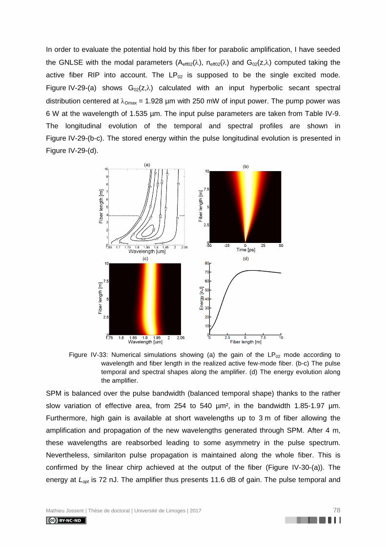
Mathieu Jossent | Thèse de doctorat | Université de Limoges | 2017 78
In order to evaluate the potential hold by this fiber for parabolic amplification, I have seeded
the GNLSE with the modal parameters (Aeff02(), neff02() and G02(z,) computed taking the
active fiber RIP into account. The LP02 is supposed to be the single excited mode.
Figure IV-29-(a) shows G02(z,) calculated with an input hyperbolic secant spectral
distribution centered at Dmax = 1.928 µm with 250 mW of input power. The pump power was
6 W at the wavelength of 1.535 µm. The input pulse parameters are taken from Table IV-9.
The longitudinal evolution of the temporal and spectral profiles are shown in
Figure IV-29-(b-c). The stored energy within the pulse longitudinal evolution is presented in
Figure IV-29-(d).
Figure IV-33: Numerical simulations showing (a) the gain of the LP02 mode according to
wavelength and fiber length in the realized active few-mode fiber. (b-c) The pulse
temporal and spectral shapes along the amplifier. (d) The energy evolution along
the amplifier.
SPM is balanced over the pulse bandwidth (balanced temporal shape) thanks to the rather
slow variation of effective area, from 254 to 540 µm², in the bandwidth 1.85-1.97 µm.
Furthermore, high gain is available at short wavelengths up to 3 m of fiber allowing the
amplification and propagation of the new wavelengths generated through SPM. After 4 m,
these wavelengths are reabsorbed leading to some asymmetry in the pulse spectrum.
Nevertheless, similariton pulse propagation is maintained along the whole fiber. This is
confirmed by the linear chirp achieved at the output of the fiber (Figure IV-30-(a)). The
energy at Lopt is 72 nJ. The amplifier thus presents 11.6 dB of gain. The pulse temporal and

Mathieu Jossent | Thèse de doctorat | Université de Limoges | 2017 79
spectral shapes at Lopt are presented in Figure IV-30-(a-b) and its maximal achieved
compression in Figure IV-30-(c).
Figure IV-34: Numerical simulations showing (a-b) the temporal and spectral shape of the
amplified pulse at Lopt. (c) The temporal profile of the recompressed pulse with
140 fs duration. The central lobe contains 55% of the output energy.
The pulse can be compressed down to 140 fs FWHM with a grating distance of 3 cm. The
central lobe contains 55% of the output energy. This leads to over 230 kW peak power. As in
6.2.2., the repetition rate was lowered to increase the amount of input energy, the results are
presented in Table IV-10.
Table IV-11: Numerical simulations showing the scalability in peak power in the active few
mode fiber for different input energy with constant average power (250 mW).
Rep_rate (MHz)
Ein (nJ)
Lopt (m)
E(Lopt) (nJ)
tcompressed (fs) Energy fraction
in central lobe (%) Peak power
(MW)
48 5.2 5.95 72 140 46 0.237
30 8.3 5.45 114 140 43 0.350
10 25 4.31 330 120 36 1
As with the optimal fiber, lowering the repetition rate to 10 MHz allowed reaching the
milestone of 1 MW peak power. This is mainly due to the low effective area variation
enabling the SPM generation over a broader spectrum compared to the optimal fiber.
In both cases, we are far from the limitations dictated by the fiber geometrical characteristics,
namely dispersion and effective area. The barrier that has to be surpassed is the fiber gain
behavior that forbids energy scaling.
IV.4. Conclusion
A singlemode Tm-doped fiber was manufactured at IRCICA-PhLAM to study the
efficiency of the glass matrix that will be further used in the active few-mode fiber. The Tm3+-
ion radial distribution had to be taken into account to allow reaching very good agreement
between the model and the measurements. An in-house (3+1)D (x,y,z and ) amplifier
software was used to model the LP02 mode gain evolution according to fiber length and
wavelength (G02(z,)). In order to push away the gain saturation, the pump wavelength has to
140 fs

Mathieu Jossent | Thèse de doctorat | Université de Limoges | 2017 80
be lowered and was thus fixed to 1.535 µm. Along the amplification, the modal weight of the
LP02 could suffer strong changes due to the low overlaps between the modes carrying the
pump and the signal. To lower the strength of the modal weight reduction it has be
demonstrated that the pump should also be carried by the LP02. Another way was studied
using an enhanced design of the fiber. The incorporation of a central dip in the RIP allowed
lowering the overlap between the gain media and the fundamental mode. This enhanced
design transfers the necessity of mode conversion at the pump wavelength to a necessity of
long pieces of fiber. The length of an amplifier based on this design can be managed by
changing the pump wavelength. Moreover this design increases the LP02 modal weight along
the amplification. This design is currently being manufactured at IRCICA-PhLAM.
Armed with these parameters, the in-house GNLSE software has been fed by several
parameters: the pulse characteristics of the SFSS source; the dispersion, the effective area
and the gain of the LP02 mode. The proposed optimal design allows reaching 0.1 µJ at Lopt.
The pulse could be recompressed to 192 fs with a central lobe containing 52 % of the energy
leading to 270 kW peak power.
A very first active few-mode fiber presenting high –D was manufactured and numerically
studied. This fiber could allow reaching over 230 kW peak power in a recompressed pulse of
140 fs. If the repetition rate is lowered all other things being equal, the 1 MW milestone can
be reached with this fiber.
Mathieu Jossent | Thèse de doctorat | Université de Limoges | 2017 81
General Conclusion and prospects
The goal of this thesis was to pave the way towards the demonstration of all-fiber
format high energy amplification at 2 µm. Parabolic amplification is a good candidate but this
amplification regime is prohibited in silica at 2 µm due to the large anomalous dispersion of
the material. Furthermore, according to eff32
2 ADgn8cΕ̂ high energy
amplification at 2 µm would need a special Tm-doped fiber with both high normal dispersion
(–D) and large effective mode area (Aeff). Waveguiding effects are inhibited by nature in large
mode area singlemode fibers thus preventing the design of single large mode area fibers
with high –D at 2 μm.
Ramachandran and coworkers [27], [29] have widely used the possibilities offered by high
order modes in terms of dispersion control in the telecom window using passive few mode
fibers. These modes exhibit high –D and large mode area near their respective cut-offs.
However, optimized designs for direct amplification to high energy in the normal dispersion
regime were never reported up to now.
In this thesis, I have presented the different steps to design a fiber that can be
manufactured by MCVD and that gathers all attributes necessary to initiate parabolic
amplification around 2 µm. The proposed fiber presented a W-like refractive index profile
(RIP) and guided the first four LP modes. The dependence of the dispersion curve of the
LP02 mode to the RIP is strong. The LP02 mode of the modeled fiber exhibits a high negative
dispersion value of D = -380 ps/(nm.km) at Dmax = 1.908 µm with a corresponding effective
mode area of 353 µm². A passive version was first realized by our partner IRCICA/PhLAM.
Despite the discrepancy between the target fiber and the realized fiber, the calculated LP02
mode of the later exhibits a dispersion value of -137 ps/(nm.km) combined with an effective
area of 393 µm² at Dmax = 1.99 µm. This fiber constitutes the first milestone towards
parabolic amplification at 2 µm. However, careful launching into the LP02 mode is necessary
to take advantage of its exceptional modal parameters at this wavelength.
Two ways to realize a selective excitation of the LP02 mode in the passive fiber have
been investigated during this thesis and are presented in the second chapter. On one hand,
the use of Long Period Gratings (LPG) was studied. A collaboration between XLIM and the
Ecole Polytechnique Fédérale de Lausanne (EPFL) in Switzerland has been established
during this thesis to manufacture LPGs in our fibers. The fiber in which the LPGs were
written presented high normal dispersion around 1.55 µm for the LP02 mode while the mode
matching between the fundamental and the LP02 modes was expected around 1.54 µm. The
first result we obtained was a 40% mode converter around 1.7 µm using a grating period of

Mathieu Jossent | Thèse de doctorat | Université de Limoges | 2017 82
170 µm. During this study I concluded that LPGs add another degree of complexity on the
RIP in order to match the mode conversion bandwidth with the high normal dispersion
bandwidth.
On the other hand, a spatial mode converter was manufactured at XLIM using the hole-
inflation technique in a PCF cane. This mode converter allowed the spatial structuration of
light from the input SMF to a LP02–like mode at its output. Contrary to LPGs, no spectral
filtering due to the conversion bandwidth was expected as the conversion was realized over
a broad spectral bandwidth of 400 nm from 1.5 µm to 1.9 µm. This spatial mode converter
thus holds potential to convert both pump and signal radiations. This mode converter was
then used to excite the passive few mode fiber sample. However, a camera image did not
allow us to conclude on the purity of excitation. During my thesis, I have implemented at
XLIM the spectrally- and spatially-resolved imaging technique (S²) as first described by
Nicholson and coworkers [33]. Using this technique on the association ‘mode
converter-passive few mode fiber’ gave state-of-the-art results in terms of purity of excitation
of a higher order mode. Parasitic modes presented multi-path interference values lower than
-35 dB at 1.55 µm and at 1.87 µm. This type of mode converter constitutes the second
milestone towards parabolic amplification at 2 µm. The output facet of the dedicated mode
converter made at XLIM was unfortunately damaged and could not be used anymore. Dr.
Correa from CREOL provided us with photonic lanterns [35]–[38] to further investigate on
high purity mode excitation. These lanterns are still under test.
As explained in Liu’s thesis [5], the amplification of parabolic pulses require the input
pulse duration to be on the order of 100 fs. To address this mater, I fabricated a pulse source
based on self-frequency shifted soliton producing 100 fs duration pulses with an average
power of 250 mW. This source is tunable from 1.6 µm to 2 µm by adjusting the pump power
of the last stage amplifier that produces the Raman-shifted soliton. This source allowed us to
measure the LP02 dispersion in the passive few mode fiber at the wavelength of 1.95 µm,
D = -106 ps/(nm.km), in very good agreement with the calculated value of -108 ps/(nm.km).
The last chapter summarizes the numerical studies on an active version of the
calculated fiber in both linear and nonlinear amplification. The glass matrix efficiency was first
measured in a singlemode Tm-doped fiber. Then, a (3+1)D (x,y,z and ) amplifier software
modeling the modal gain competition taking the transverse distribution of Tm3+-ion allowed us
to compute the spectral and longitudinal evolution of the LP02 modal gain. By design, the
dispersive fiber presents a decreasing overlap between the active-core and the LP02 mode
with wavelength. This results in deteriorating the modal purity along the amplification. A
solution (controlled dip in the Tm-doped portion of the refractive index profile) was proposed

Mathieu Jossent | Thèse de doctorat | Université de Limoges | 2017 83
to enhance the modal purity along the amplification. This fiber is being manufactured by our
partner IRCICA-PhLAM.
In the in-house GNLSE solving software were injected the spectral and longitudinal evolution
of the LP02 gain combined with both the fiber geometrical characteristics and the SFSS
source pulse parameters. The proposed optimal design allows reaching 0.1 µJ at Lopt. The
pulse could be recompressed to 192 fs with a central lobe containing 52 % of the energy
leading to 270 kW peak power.
A very first active few-mode fiber presenting high –D was manufactured and numerically
studied. This fiber could allow reaching over 230 kW peak power in a recompressed pulse of
140 fs. If the repetition rate is lowered all other things being equal, the 1 MW milestone can
be reached with this fiber.
In terms of prospects, the use of photonic lanterns as mode converters makes easy
the excitation of the LP02 mode. We are currently investigating on the photonic lanterns that
were delivered to XLIM. Their use in an ultrashort pulse laser would be a world first. Using
this device with the current active fiber might lead to a proof of concept of parabolic
amplification at 2 µm. However, the expected excitation purity with such devices is on the
order of -10 dB [37]. The association of the photonic lanterns with the enhanced design fiber
will surely produce interesting results and demonstrate the energy scaling via parabolic
amplification at 2 µm. We are also studying the homemade spatial mode converter with
special care paid to a monolithically integrated system.

Mathieu Jossent | Thèse de doctorat | Université de Limoges | 2017 84
Appendix. Experimental determination of the modal content by means of S2
imaging
The beam quality at the output of the fiber as always been thoroughly investigated. Since
standard fiber lasers operate on the fundamental mode which have a nearly Gaussian shape
the well-known M² measurement was sufficient in most cases to describe the output beam.
However, there exist situations in which the M²-parameter is low (indicating good beam
quality), yet the beam contains a significant amount of higher-order mode content [44]. The
resulting modal interference causes beam fluctuations in the far-field. With the renewed
interest on multimode fibers, other type of characterizations arose that can be sorted into two
categories. On one hand, there are methods that need a prior knowledge of the measured
fiber. From the known modal content and the output beam shape one can retrieve any weight
of each mode participating to the formation of the output pattern. Using a modal
decomposition into LP modes [45] the intensity of each modes can be retrieved. An
enhanced version have been proposed [46] using wavefront analysis so as to get the
intensity profiles and the phase of each modes constituting the output beam. On the other
hand, techniques that make no assumptions about the fiber under test have been
demonstrated. These techniques rely on the fact that the fiber modes travel at different group
velocities. Hence, one can retrieve each excited mode using a fair amount of fiber length
ensuring temporal separation of each mode. Techniques such as Spectrally- and Spatially-
resolved imaging (S²) [33], optical low-coherence interferometry [47], [48] and cross-
correlation imaging (C²) [49] are available and do require either a fixed spectral range and a
spatial sweep or a fixed spatial range and a spectral sweep. In our case, the measurement of
the modal content is to be realized over the erbium and thulium emission bandwidths on an
unknown fiber modal content. For most of the second category techniques mentioned above,
the only, and fast, way is to use a tunable laser (spectral sweep) and a CCD camera (fixed
spatial range). However, the lack of tunable lasers around 2µm and of high resolution
camera or the expansiveness of such devices forced to consider the use of a rare-earth-
based ASE source (fixed spectral range) and a 2D spatial mapping. The strength of S² relies
in the possibility to use both ways (fixed spectral range and spatial sweep or the other way
around) without the need of a reference (as opposed to C²) to perform the measurement.
S² has been demonstrated by Nicholson and coworkers [33] and rely on the
assessment that a multimode fiber guiding N modes behaves as an N unbalanced arms
interferometer. Therefore, if one arm has a dominating intensity, the resulting interferences
will be from this arm with others. Less excited arms interfering with others are neglected in
this approach. In this scenario, the produced interferograms will provide sufficient data to
enable the evaluation of the modal content at the output of any kind of fibers. In its

Mathieu Jossent | Thèse de doctorat | Université de Limoges | 2017 85
demonstration, spectral interferences were spatially resolved. Fringes in the optical spectrum
could be identified as peaks in the temporal domain through the use of Fourier transform. For
a detailed theortical explanation the reader is invited to look into ref [33], [50].
A.1. Modeling
In its basic form, S² measurement requires a preponderant mode over the others. It is
commonly used with a preponderant fundamental LP01 mode which eventually will not be our
case. Modeling is then required to foresee the possible different interference patterns since
every reconstruction and MPI evaluation will be realized with a preponderant LP02. The
following simulations model the S² measurements of the designed optimal fiber (Chapter II.4)
excited by a flat ASE source. The interference patterns are generated between 1.83 and 1.87
µm with a spectral resolution of 40 pm. Two excitation conditions are modeled with either
LP01 or LP02 being the main mode. The weight of each mode and the averaged calculated
differential group delays normalized by the fiber length (fDGDs) between the main mode and
the other modes are summed up table A-1.
Table A-IV-12: S² modeling with two distinct excitations and corresponding differential group
delays.
Mode
Main mode
LP01 LP02
Power fraction (%) fDGD (ps/m) Power fraction (%) fDGD (ps/m)
LP01 97 1 5.51
LP11 1 6.16 1 0.69
LP21 1 11.58 1 6.07
LP02 1 5.51 97
The expected MPI is equal to -19.87 dB for each mode as their weight is equal. Using
the mode solver described in Chapter II, the radial field distributions and effective indices of
each mode at every wavelength are computed. From those radial distributions are created
2D distributions normalized in intensity. A pixel by pixel interference spectrum is generated
using the computed effective indices while introducing controlled weight on each guided
mode as described by the following equations:
))(( 0),(),,( fibernmeff Lnjk
nmnmnm eyxDistAmpyxE
(A.1)
.c.c),y,x(E),y,x(Interf
esmod
nm
(A.2)
where Enm is the electrical field of the LPnm mode with the 2D distribution Distnm, Ampnm is the
square root of the fraction of power contained in the mode (given in Tab III-1), neff-nm is the
wavelength dependent effective index of the considered mode and Lfiber the simulated fiber

Mathieu Jossent | Thèse de doctorat | Université de Limoges | 2017 86
length. Interf is the generated interference spectrum which stands for the measured
spectrum in the experiment.
Inverse Fourier transform is performed at each point of the matrix which contains an
optical spectrum. Taking the modulus of the inverse Fourier transform will lead to amplitude
interference patterns while taking the phase will enable phase interference patterns.
A.1.1. Preponderant LP01 mode
The obtained temporal traces are summed so as to extract the interferences peaks
from noise. The fDGDs and interference patterns can be identified and observed at that point
(Figure A-1).
Figure A-IV-35: S² modeling - preponderant LP01: differential group delay, normalized by the
fiber length, identification with correlated 2D interference patterns in insets.
The peak at null DGD represents the superposition of all 2D interference patterns (2D-IP)
and is equivalent of what a camera could record at the fiber output.
While using the fundamental LP01 mode as the main mode, 2D-IP and reconstructed modes
produce rather similar pictures. The main difference being that the 2D-IP seems to be
compressed towards the center. The retrieved fDGDs agree well with the expected values.
Moreover, as can be seen on Figure A-1, a spurious peak can be noticed at fDGD =
0.67 ps/m. It gives a 2D-IP of the form of the LP12 mode which is not a guided mode of the
simulated fiber. This peak is consistent with the one between the LP02 and the LP11 as noted
in Tab III-1. This gives an insight of what can be expected in terms of 2D-IP in the case of a
preponderant LP02 mode.
Using the calculation of the ‘f’ and parameters the mode intensities and phases can be
reconstructed and their respective weights identified.
-50
-45
-40
-35
-30
-25
-20
-15
-10
-5
0
0 5 10 15
Differential group delay (ps/m)
Su
m o
f te
mp
ora
l tra
ce
s (
dB
)
0.67 5.44 6.07 11.39
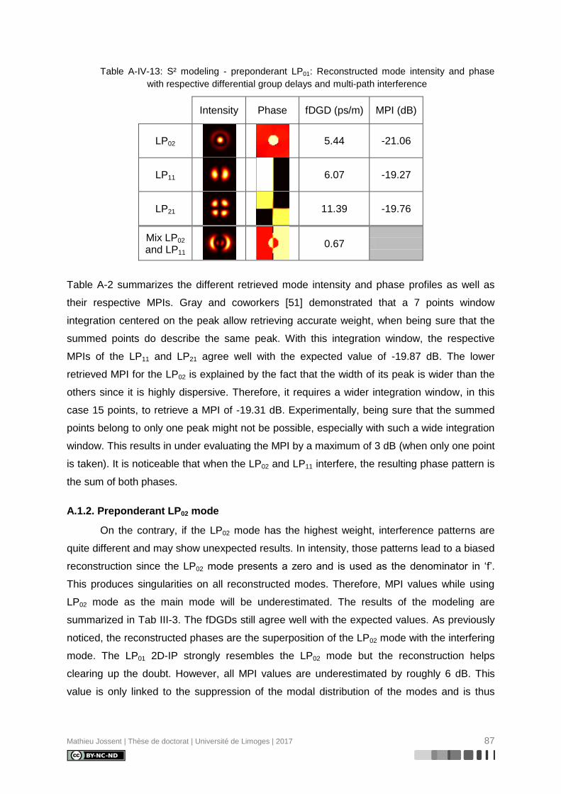
Mathieu Jossent | Thèse de doctorat | Université de Limoges | 2017 87
Table A-IV-13: S² modeling - preponderant LP01: Reconstructed mode intensity and phase
with respective differential group delays and multi-path interference
Intensity Phase fDGD (ps/m) MPI (dB)
LP02
5.44 -21.06
LP11
6.07 -19.27
LP21
11.39 -19.76
Mix LP02 and LP11
0.67
Table A-2 summarizes the different retrieved mode intensity and phase profiles as well as
their respective MPIs. Gray and coworkers [51] demonstrated that a 7 points window
integration centered on the peak allow retrieving accurate weight, when being sure that the
summed points do describe the same peak. With this integration window, the respective
MPIs of the LP11 and LP21 agree well with the expected value of -19.87 dB. The lower
retrieved MPI for the LP02 is explained by the fact that the width of its peak is wider than the
others since it is highly dispersive. Therefore, it requires a wider integration window, in this
case 15 points, to retrieve a MPI of -19.31 dB. Experimentally, being sure that the summed
points belong to only one peak might not be possible, especially with such a wide integration
window. This results in under evaluating the MPI by a maximum of 3 dB (when only one point
is taken). It is noticeable that when the LP02 and LP11 interfere, the resulting phase pattern is
the sum of both phases.
A.1.2. Preponderant LP02 mode
On the contrary, if the LP02 mode has the highest weight, interference patterns are
quite different and may show unexpected results. In intensity, those patterns lead to a biased
reconstruction since the LP02 mode presents a zero and is used as the denominator in ‘f’.
This produces singularities on all reconstructed modes. Therefore, MPI values while using
LP02 mode as the main mode will be underestimated. The results of the modeling are
summarized in Tab III-3. The fDGDs still agree well with the expected values. As previously
noticed, the reconstructed phases are the superposition of the LP02 mode with the interfering
mode. The LP01 2D-IP strongly resembles the LP02 mode but the reconstruction helps
clearing up the doubt. However, all MPI values are underestimated by roughly 6 dB. This
value is only linked to the suppression of the modal distribution of the modes and is thus

Mathieu Jossent | Thèse de doctorat | Université de Limoges | 2017 88
independent of the excitation conditions. Therefore, in any further MPI measurements
involving the LP02 mode as the preponderant one, MPI values will be corrected by +6 dB.
Table A-IV-14: S² modeling - preponderant LP02: 2D interference patterns, reconstructed mode
intensity and phase with respective differential group delays and multi-path
interference
2D-IP Intensity Phase fDGD (ps/m) MPI (dB)
LP11
0.63 -25.55
LP01
5.44 -25.01
LP21
5.95 -25.24
A.1.3. Water absorption influence
In the S² measurement, the biggest temporal window requires the smallest spectral
step. This will allow the resolution of thin absorption peaks of any airborne components
present in the spectrum analyzer or in free space. Working in the thulium emission bandwidth
has proven to be difficult in free space due to water absorption peaks. Gaida and coworkers
[21] have put their CPA in a controlled climate chamber ensuring a very low humidity to
achieve proper compression. If not regulated, the air humidity is roughly of 25%. The free
space optical path in an optical spectrum analyzer is around 1 m. When considering those
two parameters, the water contribution to spectrum is as follows (Figure A-2).
Figure A-IV-36: Water transmission from 1.82 µm to 1.88 µm in a 1 m gaz cell with 25%
humidity (http://spectralcalc.com/).
The water contribution to spectrum was implemented at the spectrum generation step hence modifying
the Equation A.2:
.c.c),y,x(E*Water),y,x(Interf
esmod
nm (A.3)
0
0.1
0.2
0.3
0.4
0.5
0.6
0.7
0.8
0.9
1
1.82 1.83 1.84 1.85 1.86 1.87 1.88
Wavelength (µm)
No
rma
lize
d w
ate
rtr
an
sm
issio
n
-40
-35
-30
-25
-20
-15
-10
-5
0
0 5 10 15 20
Delay (ps/m)
Inve
rse
Fo
uri
er
tra
nsfo
rmo
f w
ate
r tr
an
sm
issio
n

Mathieu Jossent | Thèse de doctorat | Université de Limoges | 2017 89
where Water() is the transmission spectrum of Figure A-3-(a). For example, in the case of
the LP02 mode being preponderant, the shape of the sum of temporal traces and of
reconstructed modes are strongly changed by water contribution as shown in Figure A-3-(b).
(a) (b)
Water? Peak 1 Peak 2 Peak 3
Without
With
Figure A-IV-37: (a) Sum of temporal traces in the case where the LP02 mode is preponderant
with and without water contribution. Labeled peaks refer to interferences with the
LP02 mode (b) Comparison of the reconstructed modal intensities.
The MPIs are close to the modeled ones in the ‘without water’ case with a difference
between ±1dB. Water contribution to the S² results can be numerically compensated by
dividing the measured spectra by the properly scaled water transmission spectra.
Unfortunately, during the acquisition time the hygrometry is subject to change and without an
accurate measurement the compensation cannot be done. Recently, several complementary
algorithms were proposed to allow mode reconstruction without the need of a preponderant
mode [52] or to be able to separate the 2D-IP according to the involved modes [53]. These
algorithms are yet to be implemented. Nevertheless, in the following experiments, the ‘basic’
S² algorithm was enough since we stayed in a preponderant mode excitation scheme.
A.2. S² experiments
As mention before, S² can be realized in two ways. In the first way, spatial
interferences are spectrally-resolved hence the required devices are: a tunable laser with the
lowest spectral linewidth to enable the largest temporal frame window, a CCD camera. This
way is faster but extra care has to be taken in the data post-processing since the camera
sampling rate may cause distortion in the retrieved signal [51]. However, high resolution CCD
cameras working around 2µm are not that easy to find and tunable lasers on the same
bandwidth are quite expensive. In the second way, spectral interferences are spatially-
resolved: a broadband white light source and an optical spectrum analyzer are required. In
the following, I will present the spatially-resolved spectral interferences bench that I have
created and fully automated through the use of LabView. Afterwards, modal content
measurements on the passive few-mode fiber will be presented. It will be followed by the S²
measurement of the active few-mode fiber completed by a GNLSE solving in the case of the
-60
-50
-40
-30
-20
-10
0
0 5 10 15 20
Differential group delay (ps/m)
Su
m o
f te
mp
ora
l tra
ce
s (
dB
)
With water
Without water1 2 3

Mathieu Jossent | Thèse de doctorat | Université de Limoges | 2017 90
LP02 carrying a pulse in this fiber. Another measurement of a Tm-doped LMA will be
presented to show the flexibility of the developed bench.
A.2.1. S² setup
The bench is composed by three distinct parts depicted in Figure A-4:
The all-fiber polarized output ASE source, Erbium and Thulium based ASE
sources are currently available in the lab.
The fiber under test (FUT), spliced to the ASE source, and its collimated
output
The automated scanning platform and optical spectrum analyzer.
Figure A-IV-38: Spectrally- and spatially-resolved imaging bench scheme.
The ASE sources emit tens of mW of power with broadband spectrum to ensure good
temporal resolution. The collimation is ensured by an achromatic set of lenses. The free
space part is kept as short as possible to lower the water contribution to the measured
spectra. The scanning platform has a 10 µm step resolution with a displacement width of 4
mm in 3D. The spatial resolution is set by the probe single mode fiber core diameter (in
green in Figure A-4). By experience, the displacement step should not exceed 1.5 times the
core diameter of the probe fiber to ensure resolution of the modal intensities close to zero.
The spectral step is taken to be the shortest available on the OSA (0.05 nm ≈ 120 ps
window) to achieve the widest temporal window. If the total DGD should be above 120 ps,
aliasing will happen and can superimpose different DGD peaks. The spectral window is
commonly taken around 30 nm (≈280 fs step), but if small DGDs (or close to zero) are to be
measured, a wider window as to be taken. The limiting parameter on a pixel measurement in
terms of time is the acquisition of the spectrum. As an example, a 51x51 pixels measurement
with a 50 nm spectral window and 0.05 nm spectral resolution has 2 hours of acquisition
time.
X
Z
Y

Mathieu Jossent | Thèse de doctorat | Université de Limoges | 2017 91
A.2.2. Passive FMF Modal content
The measurement was realized with successively 10 and 20 of fiber to allow retrieving
every guided mode. The two pieces of FMF were badly spliced at the output of the in-house
Tm-ASE source to ensure multimode excitation. The measurements were carried between
1860 and 1880 nm. Figure A-5 shows the reconstructed excited modes and their respective
fDGD for both fiber lengths. In both measurements, the LP11 fDGD is around 6.4 ps/m. The
thinner peaks in Figure A-5-(b) are due the normalization by the fiber length creating a twice
smaller temporal step. With 10 m of the passive FMF, the LP02 could not be retrieved. There
are two possible explanations. First, the excitation value is lower than the noise brought by
water. Second, the LP02 was not excited in this experiment. The LP21 is retrieved at an fDGD
around 11 ps/m. With 20 m of fiber, the LP02 mode is reconstructed contrary to the LP21. The
dispersive LP02 mode has a measured fDGD of roughly 5.2 ps/m. In Figure A-5-(b), two
degenerate LP11 modes were retrieved contrary to Figure A-5-(a). The difference in peak
height is due to the polarized characteristic of the ASE source. This is consistent with the
plateau formation of not temporally resolved degenerated modes reported by Nicholson and
coworkers [50]. Those two modes could be observed thanks to the long piece of fiber used
allowing enough accumulated group delay difference between the degenerated modes.
Figure A-IV-39: S² measurement of the passive few-mode fiber for (a) 10 m and (b) 20 m of
length.
I was able to calculate the fDGDs of the guided modes in the passive few mode fiber by
feeding the in-house mode solver with its measured refractive index profile. Table A-4
summarizes both measured and calculated fDGDs.
Table A-IV-15: Comparison of the measured by S² and calculated differential group delays in
ps/m for the passive few mode fiber.
Measured fDGDs (ps/m) Calculated fDGDs (ps/m)
LP01-11 6.4 6.16
LP01-21 11 11.58
LP01-02 5.2 5.51
-35
-30
-25
-20
-15
-10
-5
0
0 2 4 6 8 10 12
Differential group delay (ps/m)
Su
m o
f sp
ectr
al t
race
s (
dB
)
(a)
-35
-30
-25
-20
-15
-10
-5
0
0 2 4 6 8 10 12
Differential group delay (ps/m)
Su
m o
f sp
ectr
al t
race
s (
dB
)
(b)

Mathieu Jossent | Thèse de doctorat | Université de Limoges | 2017 92
The measured fDGDs agree well with the computed values. Even though the differential
group delays are wavelength dependent, the S² measurement can still be applied and
produces results with good agreement with fDGDs.
A.2.3. Active FMF
To measure the modal content of the active few mode fiber, the test bench was
modified to include a pumping stage to the thulium doped fiber under test as shown in
Figure A-6-(a). 5 meters of the active FMF were used in this experiment; it required a 750
mW pumping to ensure a gain close to 1 dB at the output. As demonstrated in the linear
modeling (IV.2), the modal weights along amplification vary. Therefore, the measured
weights are only the output weights. It is not possible to know the exact excitation condition
by just applying the loss coefficient. The output spectrum was centered at a longer
wavelength due to short wavelengths absorption by thulium ions. However, the S²
measurement was realized over a bandwidth that overlaps between input and output spectra
(Figure A-6-(b)) to ensure measuring excited modes and not distributed excitation of modes.
(a)
(b)
Figure A-IV-40: (a) S² setup for an active fiber. WDM: Wavelength division multiplexer. (b)
Spectrum at the output of the WDM (blue) and of the active FMF (red). The S²
measurement window is marked by the green surface.
In Figure A-6-(b), both spectrum present features due to water absorption in this wavelength
range.
Only two degenerated LP11 modes could be retrieved in these experiments. Higher
order modes were not well enough excited and/or amplified to be recovered as it is shown in
Figure III-8. The measured fDGD of the first LP11 mode is 1.3 ps/m which is consistent with
the calculated value of 1.23 ps/m. This shows that the LP11 was excited at the splice between
the WDM and the active FMF and not during a possible coupling along the fiber.
0
0.2
0.4
0.6
0.8
1
1.8 1.85 1.9 1.95 2
Wavelength (µm)
No
rma
lize
d in
ten
sity
WDM
FMF
S² window
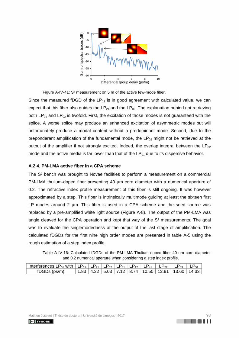
Mathieu Jossent | Thèse de doctorat | Université de Limoges | 2017 93
Figure A-IV-41: S² measurement on 5 m of the active few-mode fiber.
Since the measured fDGD of the LP11 is in good agreement with calculated value, we can
expect that this fiber also guides the LP21 and the LP02. The explanation behind not retrieving
both LP21 and LP02 is twofold. First, the excitation of those modes is not guaranteed with the
splice. A worse splice may produce an enhanced excitation of asymmetric modes but will
unfortunately produce a modal content without a predominant mode. Second, due to the
preponderant amplification of the fundamental mode, the LP02 might not be retrieved at the
output of the amplifier if not strongly excited. Indeed, the overlap integral between the LP02
mode and the active media is far lower than that of the LP01 due to its dispersive behavior.
A.2.4. PM-LMA active fiber in a CPA scheme
The S² bench was brought to Novae facilities to perform a measurement on a commercial
PM-LMA thulium-doped fiber presenting 40 µm core diameter with a numerical aperture of
0.2. The refractive index profile measurement of this fiber is still ongoing. It was however
approximated by a step. This fiber is intrinsically multimode guiding at least the sixteen first
LP modes around 2 µm. This fiber is used in a CPA scheme and the seed source was
replaced by a pre-amplified white light source (Figure A-8). The output of the PM-LMA was
angle cleaved for the CPA operation and kept that way of the S² measurements. The goal
was to evaluate the singlemodedness at the output of the last stage of amplification. The
calculated fDGDs for the first nine high order modes are presented in table A-5 using the
rough estimation of a step index profile.
Table A-IV-16: Calculated fDGDs of the PM-LMA Thulium doped fiber 40 um core diameter
and 0.2 numerical aperture when considering a step index profile.
Interferences LP01 with LP11 LP21 LP02 LP31 LP12 LP41 LP22 LP03 LP51
fDGDs (ps/m) 1.83 4.22 5.03 7.12 8.74 10.50 12.91 13.60 14.33
-30
-25
-20
-15
-10
-5
0
0 2 4 6 8 10
Differential group delay (ps/m)S
um
of sp
ectr
al t
race
s (
dB
)

Mathieu Jossent | Thèse de doctorat | Université de Limoges | 2017 94
(a) (b)
Figure A-IV-42: (a) S² setup for the PM-LMA fiber used in a CPA scheme by Novae. (b) S²
measurement results with two identified higher order modes: LP11 and LP31.
Two major observations can be made when looking at the reconstructed modes in
Figure A-8-(b). First, the angle cleave does not jeopardize the reconstruction. Second, the
retrieved fDGDs are close to the calculated ones even though a basic step index profile was
considered. The LP11 presents a MPI value of -13 dB while the LP31 one is of -25 dB. The
LP31 is not well defined in terms of intensity due to high reconstructed intensity in the corners
of the figure. However the phase information allows clearing the doubt. Other peaks present
intensity patterns with the same reconstruction issue as the LP31, however their phases are
not as well defined. Therefore, we can say that this linear excitation produces at least 6% of
power in the higher order modes. Experiments are still ongoing to assess the impact of the
presence of the higher order mode in the CPA regime.
-20
-15
-10
-5
0
0 2.5 5 7.5 10 12.5 15
Differential group delay (ps/m)
Su
m o
f sp
ectr
al t
race
s (
dB
)

Mathieu Jossent | Thèse de doctorat | Université de Limoges | 2017 95
References
[1] K. S. Kim, W. A. Reed, K. W. Quoi, and R. H. Stolen, ‘Measurement of the nonlinear index of silica-core and dispersion-shifted fibers’, Opt. Lett., vol. 19, no. 4, pp. 257–259, Feb. 1994.
[2] A. B. Grudinin, E. M. Dianov, D. V. Korbkin, A. M. Prokhorov, and D. V. Khaidarov, ‘Nonlinear mode coupling in multimode optical fibers; excitation of femtosecond-range stimulated-Raman-scattering solitons’, JETP Lett., vol. 47, no. 6, p. 356, Mar. 1988.
[3] Y. Tang, L. G. Wright, K. Charan, T. Wang, C. Xu, and F. W. Wise, ‘Generation of intense 100 fs solitons tunable from 2 to 4.3 μm in fluoride fiber’, Optica, vol. 3, no. 9, p. 948, Sep. 2016.
[4] I. H. Malitson, ‘Interspecimen Comparison of the Refractive Index of Fused Silica*,†’, JOSA, vol. 55, no. 10, pp. 1205–1209, Oct. 1965.
[5] H. Liu, ‘Development Of Fiber Lasers That Generate Few-Cycle Optical Pulses’, May 2014.
[6] N. G. Horton et al., ‘In vivo three-photon microscopy of subcortical structures within an intact mouse brain’, Nat. Photonics, vol. 7, no. 3, pp. 205–209, Mar. 2013.
[7] A. B. Grudinin and S. Gray, ‘Passive harmonic mode locking in soliton fiber lasers’, JOSA B, vol. 14, no. 1, pp. 144–154, Jan. 1997.
[8] A. Chong, J. Buckley, W. Renninger, and F. Wise, ‘All-normal-dispersion femtosecond fiber laser’, Opt. Express, vol. 14, no. 21, p. 10095, 2006.
[9] H. Wang et al., ‘Dissipative Soliton Generation and Amplification in Erbium-Doped Fibers Operating at 1.55 µm’, IEEE J. Sel. Top. Quantum Electron., vol. 20, no. 5, pp. 283–289, Sep. 2014.
[10] Y. Tang, A. Chong, and F. W. Wise, ‘Generation of 8 nJ pulses from a normal-dispersion thulium fiber laser’, Opt. Lett., vol. 40, no. 10, p. 2361, May 2015.
[11] W. H. Renninger, A. Chong, and F. W. Wise, ‘Self-similar pulse evolution in an all-normal-dispersion laser’, Phys. Rev. A, vol. 82, no. 2, p. 021805, Aug. 2010.
[12] M. E. Fermann, V. I. Kruglov, B. C. Thomsen, J. M. Dudley, and J. D. Harvey, ‘Self-Similar Propagation and Amplification of Parabolic Pulses in Optical Fibers’, Phys. Rev. Lett., vol. 84, no. 26, pp. 6010–6013, Jun. 2000.
[13] Y. Zaouter et al., ‘Stretcher-free high energy nonlinear amplification of femtosecond pulses in rod-type fibers’, Opt. Lett., vol. 33, no. 2, p. 107, Jan. 2008.
[14] A. Ruehl, H. Hundertmark, D. Wandt, C. Fallnich, and D. Kracht, ‘0.7 W all-fiber Erbium oscillator generating 64 fs wave breaking-free pulses’, Opt. Express, vol. 13, no. 16, pp. 6305–6309, Aug. 2005.
[15] J. Peng et al., ‘All-fiber ultrashort similariton generation, amplification, and compression at telecommunication band’, JOSA B, vol. 29, no. 9, pp. 2270–2274, Sep. 2012.
[16] D. S. Chernykh et al., ‘Hybrid mode-locked erbium-doped all-fiber soliton laser with a distributed polarizer’, Appl. Opt., vol. 53, no. 29, pp. 6654–6662, Oct. 2014.
[17] K.-C. Chu, H.-Y. Jiang, and S.-D. Yang, ‘High-energy femtosecond amplifier-similariton Er-doped fiber oscillator’, Opt. Lett., vol. 40, no. 22, pp. 5319–5322, Nov. 2015.
[18] D. Strickland and G. Mourou, ‘Compression of amplified chirped optical pulses’, Opt. Commun., vol. 55, no. 6, pp. 447–449, Oct. 1985.

Mathieu Jossent | Thèse de doctorat | Université de Limoges | 2017 96
[19] T. Eidam et al., ‘Fiber chirped-pulse amplification system emitting 3.8 GW peak power’, Opt. Express, vol. 19, no. 1, pp. 255–260, Jan. 2011.
[20] F. Röser et al., ‘Millijoule pulse energy high repetition rate femtosecond fiber chirped-pulse amplification system’, Opt. Lett., vol. 32, no. 24, pp. 3495–3497, Dec. 2007.
[21] C. Gaida, M. Gebhardt, F. Stutzki, C. Jauregui, J. Limpert, and A. Tünnermann, ‘Thulium-doped fiber chirped-pulse amplification system with 2 GW of peak power’, Opt. Lett., vol. 41, no. 17, pp. 4130–4133, Sep. 2016.
[22] F. Röser et al., ‘90 W average power 100 μJ energy femtosecond fiber chirped-pulse amplification system’, Opt. Lett., vol. 32, no. 15, pp. 2230–2232, Aug. 2007.
[23] D. Gaponov, L. Lavoute, S. Février, A. Hideur, and N. Ducros, ‘2µm all-fiber dissipative soliton master oscillator power amplifier’, 2016, p. 972834.
[24] F. Tan, H. Shi, R. Sun, P. Wang, and P. Wang, ‘1 μJ, sub-300 fs pulse generation from a compact thulium-doped chirped pulse amplifier seeded by Raman shifted erbium-doped fiber laser’, Opt. Express, vol. 24, no. 20, pp. 22461–22468, Oct. 2016.
[25] B. Oktem, C. Ülgüdür, and F. Ö. Ilday, ‘Soliton–similariton fibre laser’, Nat. Photonics, vol. 4, no. 5, pp. 307–311, May 2010.
[26] C. D. Poole, J. M. Wiesenfeld, A. R. McCormick, and K. T. Nelson, ‘Broadband dispersion compensation by using the higher-order spatial mode in a two-mode fiber’, Opt. Lett., vol. 17, no. 14, p. 985, Jul. 1992.
[27] S. Ramachandran, J. m. Fini, M. Mermelstein, J. w. Nicholson, S. Ghalmi, and M. f. Yan, ‘Ultra-large effective-area, higher-order mode fibers: a new strategy for high-power lasers’, Laser Photonics Rev., vol. 2, no. 6, pp. 429–448, Dec. 2008.
[28] X. Peng et al., ‘Higher-order mode fiber enables high energy chirped-pulse amplification’, Opt. Express, vol. 21, no. 26, pp. 32411–32416, Dec. 2013.
[29] S. Ramachandran, ‘Dispersion-Tailored Few-Mode Fibers: A Versatile Platform for In-Fiber Photonic Devices’, J. Light. Technol., vol. 23, no. 11, p. 3426, Nov. 2005.
[30] A. E. Miller, R. L. Opila, and M. F. Yan, ‘Ultranegative delta cladding for modified chemical vapor deposition’, 1996, pp. 56–58.
[31] G. Humbert and A. Malki, ‘Electric-arc-induced gratings in non-hydrogenated fibres: fabrication and high-temperature characterizations’, J. Opt. Pure Appl. Opt., vol. 4, no. 2, p. 194, 2002.
[32] K. Lai, S. G. Leon-Saval, A. Witkowska, W. J. Wadsworth, and T. A. Birks, ‘Wavelength-independent all-fiber mode converters’, Opt. Lett., vol. 32, no. 4, pp. 328–330, Feb. 2007.
[33] J. W. Nicholson, A. D. Yablon, S. Ramachandran, and S. Ghalmi, ‘Spatially and spectrally resolved imaging of modal content in large-mode-area fibers’, Opt. Express, vol. 16, no. 10, pp. 7233–7243, May 2008.
[34] F. Morin, Conception d’une source à impulsions courtes à 1600 nm à fibres dopées erbium : application à la greffe de cornée. Paris 11, 2010.
[35] S. G. Leon-Saval, N. K. Fontaine, J. R. Salazar-Gil, B. Ercan, R. Ryf, and J. Bland-Hawthorn, ‘Mode-selective photonic lanterns for space-division multiplexing’, Opt. Express, vol. 22, no. 1, pp. 1036–1044, Jan. 2014.
[36] T. A. Birks, I. Gris-Sánchez, S. Yerolatsitis, S. G. Leon-Saval, and R. R. Thomson, ‘The photonic lantern’, Adv. Opt. Photonics, vol. 7, no. 2, p. 107, Jun. 2015.
[37] A. M. Velazquez-Benitez et al., ‘Six mode selective fiber optic spatial multiplexer’, Opt. Lett., vol. 40, no. 8, pp. 1663–1666, Apr. 2015.
Mathieu Jossent | Thèse de doctorat | Université de Limoges | 2017 97
[38] G. Lopez-Galmiche et al., ‘Few-mode erbium-doped fiber amplifier with photonic lantern for pump spatial mode control’, Opt. Lett., vol. 41, no. 11, pp. 2588–2591, Jun. 2016.
[39] M. A. Khamis and K. Ennser, ‘Theoretical Model of a Thulium-Doped Fiber Amplifier Pumped at 1570 nm and 793 nm in the Presence of Cross Relaxation’, J. Light. Technol., vol. 34, no. 24, pp. 5675–5681, Dec. 2016.
[40] P. Peterka, I. Kasik, A. Dhar, B. Dussardier, and W. Blanc, ‘Theoretical modeling of fiber laser at 810 nm based on thulium-doped silica fibers with enhanced ^3H_4 level lifetime’, Opt. Express, vol. 19, no. 3, p. 2773, Jan. 2011.
[41] S. D. Agger and J. H. Povlsen, ‘Emission and absorption cross section of thulium doped silica fibers’, Opt. Express, vol. 14, no. 1, p. 50, 2006.
[42] S. D. Jackson and T. A. King, ‘Theoretical modeling of Tm-doped silica fiber lasers’, J. Light. Technol., vol. 17, no. 5, pp. 948–956, May 1999.
[43] M. DEVAUTOUR, ‘Étude de fibres actives combinant large cœur et fort niveau de dopage pour l’émission unimodale ’:, thesis, Université de Limoges.
[44] S. Wielandy, ‘Implications of higher-order mode content in large mode area fibers with good beam quality’, Opt. Express, vol. 15, no. 23, pp. 15402–15409, Nov. 2007.
[45] D. B. S. Soh, J. Nilsson, S. Baek, C. Codemard, Y. Jeong, and V. Philippov, ‘Modal power decomposition of beam intensity profiles into linearly polarized modes of multimode optical fibers’, JOSA A, vol. 21, no. 7, pp. 1241–1250, Jul. 2004.
[46] M. Paurisse, L. Lévèque, M. Hanna, F. Druon, and P. Georges, ‘Complete measurement of fiber modal content by wavefront analysis’, Opt. Express, vol. 20, no. 4, pp. 4074–4084, Feb. 2012.
[47] Y. Ma, ‘Characterization of Higher Order Modes in Optical Fibers, Charakterisierung von Moden höherer Ordnung in optischen Fasern’.
[48] Y. Z. Ma et al., ‘Fiber-modes and fiber-anisotropy characterization using low-coherence interferometry’, Appl. Phys. B, vol. 96, no. 2–3, pp. 345–353, Aug. 2009.
[49] D. N. Schimpf, R. A. Barankov, and S. Ramachandran, ‘Cross-correlated (C2) imaging of fiber and waveguide modes’, Opt. Express, vol. 19, no. 14, pp. 13008–13019, Jul. 2011.
[50] J. W. Nicholson, A. D. Yablon, J. M. Fini, and M. D. Mermelstein, ‘Measuring the Modal Content of Large-Mode-Area Fibers’, IEEE J. Sel. Top. Quantum Electron., vol. 15, no. 1, pp. 61–70, Jan. 2009.
[51] D. R. Gray et al., ‘Accurate calibration of S^2 and interferometry based multimode fiber characterization techniques’, Opt. Express, vol. 23, no. 8, p. 10540, Apr. 2015.
[52] H. Otto, F. Jansen, F. Stutzki, C. Jauregui, J. Limpert, and A. Tunnermann, ‘Improved Modal Reconstruction for Spatially and Spectrally Resolved Imaging’, J. Light. Technol., vol. 31, no. 8, pp. 1295–1299, Apr. 2013.
[53] B. Sévigny et al., ‘Advanced S Imaging: Application of Multivariate Statistical Analysis to Spatially and Spectrally Resolved Datasets’, J. Light. Technol., vol. 32, no. 23, pp. 4606–4612, Dec. 2014.

Mathieu Jossent | Thèse de doctorat | Université de Limoges | 2017 98
Table of figures
Figure I-1: Simulated electrical field oscillations of a laser pulse inside a fiber. The intensity
variation is represented by the pulse envelope. (a) Input pulse. (b) Output pulse. (c) Spectra
for the input pulse (blue) and the is output pulse (green), showing spectral broadening by
the optical Kerr effect............................................................................................................. 4
Figure I-2: Stimulated Raman Scattering - Energy diagram of the generation of Stokes and
Anti-stokes waves. ................................................................................................................ 5
Figure I-3: Imaginary part of the Raman susceptiblity (=Raman gain in arbitrary units) in a
SiO2 core fiber. ...................................................................................................................... 6
Figure I-4: Silica dispersion curve calculated by Sellmeier series from [4]. Dispersion values
at commonly used lasing wavelengths: Ytterbium 1.03 µm (blue), Erbium 1.55 µm (green)
and Thulium 1.9 µm (red). ..................................................................................................... 8
Figure I-5: Diagram of the symmetrized split-step Fourier method. Dispersive operator is
applied over [z;z+h/2[ and ]z+h/2;z+h[. Nonlinear operator is applied at z+h/2. ....................10
Figure I-6: Illustration of self similar evolution of the temporal (left) and spectral (right) shapes
of a similariton along its amplification. ..................................................................................13
Figure I-7: Calculated maximal extractible energy, before wavebreaking, of an amplified
similariton centered at 1.9 µm as a function of the absolute value of the dispersion coefficient
for various modal effective areas. .........................................................................................14
Figure I-8: Experimental setup of a CPA [21]. (AOM: Acousto-optic modulator, PCF: Photonic
crystal fiber, LPF: Large pitch rod-type fiber). .......................................................................16
Figure I-9: Experimental spectrum measurements: (a) before two stages of amplification
(yellow) and at the output of the main amplifier (purple) by Gaida and coworkers [21], (b)
main amplifier input (black) and output (red) by Eidam and coworkers [19]. .........................17
Figure II-1: Principle of operation of a moderately multimode fiber for dispersion control. Top:
Generic profile of a step-index moderately multimode fiber. Associated LP02 intensity profile.
Middle: LP02 mode effective index versus wavelength. Insets show the field spreading when
increases. Bottom: LP02 dispersion versus wavelength. ........................................................24
Figure II-2: Principle of operation of an improved design of a few mode fiber for dispersion
control. Top: Generic index profile of a few mode fiber. Associated LP02 intensity profile.
Middle: LP02 mode effective index (thick black curve) is a linear combination of the ‘core’
mode and of the ‘ring’ mode. The inflexion causes high –DW around the phase-matching
point. The effective index of the LP02 is increased above the silica index ensuring low loss
guidance. Bottom: LP02 dispersion versus wavelength. The additional features (trench, ring)
help tailor the dispersion and dispersion slope. ....................................................................25
Figure II-3: (a) LP02 mode profile at the most dispersive wavelength (solid line) in a few mode
fiber (RIP: gray background). (b) Corresponding plot of LP02 dispersion versus wavelength.
λcut-off represents the wavelength at which the LP02 mode leaks in the cladding [29]. ............26
Figure II-4: The various parameters of a typical few mode fiber for dispersion control. .........26
Figure II-5: The various LP0m, in intensity, of a typical few mode fiber for dispersion control
with their effective index position according to the RIP. ........................................................28

Mathieu Jossent | Thèse de doctorat | Université de Limoges | 2017 99
Figure II-6: Impact of the ring thickness r3 on the dispersion spectrum. ..............................29
Figure II-7: Impact of the ring index difference n3 on the dispersion spectrum. ...................30
Figure II-8: Impact of the trench thickness r2 on the dispersion spectrum. ..........................30
Figure II-9: Impact of the trench index difference n2 on the dispersion spectrum. ...............31
Figure II-10: Chromatic dispersion of the designed RIP versus wavelength. Inset: RIP for
improved dispersion. α = 6, n1 = 1510–3, r1 = 8 µm, n2 = –410–3, r2 = 4 µm, n3 = 310–
3, r3 = 8 µm. ........................................................................................................................32
Figure II-11: (a) Measured refractive index difference of the passive (blue) few mode fiber.
Black line shows the target RIP. (b) Dispersion curves computed for the two RIPs shown in
(a).........................................................................................................................................33
Figure III-1: Scheme of a high-order mode based amplifier. Light propagating in the LP01
mode of the input fiber is converted to a high normal dispersion high-order mode of a few
mode fiber, the LP02 mode for instance.................................................................................34
Figure III-2: Waveguide dispersion versus wavelength for the LP02 mode of dispersive few
mode fiber. Transmission of the LPG (dotted curve) versus wavelength on the right scale.
= 206.9 µm. .......................................................................................................................35
Figure III-3: Group indices of the LP02 and LP01 (dotted curve) modes versus wavelength. ...36
Figure III-4: Group indices of the LP02 and LP01 (dotted) modes versus wavelength in a
dispersive few mode fiber adapted for LPG inscription. ........................................................37
Figure III-5: Waveguide dispersion versus wavelength in a dispersive few mode fiber adapted
for LPG inscription. Transmission of the LPG (dotted curve) versus wavelength on the right
scale. = 413.4 µm. ............................................................................................................37
Figure III-6: (a) Measured refractive index difference of the 1.5 µm-FMF and (b) Calculated
group index of the LP01 (black) and LP02 (red) modes. ..........................................................38
Figure III-7: (a) Evolution of FBG transmission according to time in the 1.5 µm-FMF. (b) FBG
transmission spectrum at t = 1690 s) ....................................................................................38
Figure III-8: OLCR spectrum of 1.55 µm-FMF end reflection measured with 1560 nm source.
.............................................................................................................................................39
Figure III-9: Cut back measurement of LP01 OLCR peak of 1.55 µm-FMF. ...........................39
Figure III-10: (a) Measured transmission loss spectrum indicating a LP01-LP02 mode
converter around 1.7 µm for a 2 cm LPG with around 170 µm pitch. (b) Simulated
transmission loss spectrum for a 2 cm LPG with a 171.2 µm pitch .......................................40
Figure III-11: Top, Schematic longitudinal cross section of the inflation-based mode
converter, showing core areas in dark gray. Bottom: optical micrographs of the holey region
in the cleaved fiber in each of sections A–D, on the same scale. From [32]. .........................41
Figure III-12: Measured near field output at = 1 µm. From [32]. .........................................42
Figure III-13: Computed effective indexes of the ‘LP01’ ring mode and the ‘LP02’ of the
adiabatic mode converter versus the diameter of the six internal holes. Insets represent the
intensity profile for each mode. Insets 1–7 show the internal modification of the guiding
structure. ..............................................................................................................................43

Mathieu Jossent | Thèse de doctorat | Université de Limoges | 2017 100
Figure III-14: Computed normalized electric field amplitudes for the LP02 mode of the
converter and the LP01 and LP02 modes of the few mode fiber. The inset is the computed
intensity of the LP02 mode of the converter. ..........................................................................43
Figure III-15: Fabrication of a holey preform (or cane). .........................................................44
Figure III-16: Operation principle of the manufacturing of the mode converter. .....................44
Figure III-17: (a) Micrograph of the holey cane used to manufacture the adiabatic converter.
(b) Micrograph of the output end facet of the manufactured converter. .................................45
Figure III-18: Near field output of the mode converter excited by (a) an Erbium ASE source
and (b) a Thulium ASE source. .............................................................................................45
Figure III-19: Radial scan of the output near field of the mode converter excited by (a) the
Erbium ASE source with 41 points of measurements and (b) the Thulium ASE source with
101 points of measurements. (c) and (d) are the respective radial traces at the beginning and
the end of both bandwidths...................................................................................................46
Figure III-20: Experimental set-up to evaluate selective modal excitation of the passive few
mode fiber. ...........................................................................................................................46
Figure III-21: Near field output of the passive few-mode fiber when excited by the mode
converter with (a) the Erbium ASE source and (b) the Thulium ASE source. ........................47
Figure III-22: S² measurement of the passive few-mode fiber excited by the mode converter
on the Erbium emission bandwidth for 20 m of fiber. 3 retrieved parasitic modes: LP21, LP31
and LP11. ..............................................................................................................................48
Figure III-23: S² measurement of the passive few-mode fiber excited by the mode converter
within the Thulium emission bandwidth for 20 m of fiber. Only one retrieved parasitic mode:
LP11. .....................................................................................................................................49
Figure III-24: Setup scheme for the self-frequency shifted soliton source. Upper line is the
temporal shape along the setup with colors representing the pulse chirp (grey stands for
chirp equal to 0). Standard singlemode (SM) fibers are represented in yellow, multimode
(MM) fibers in dark yellow. HNLF highly nonlinear fiber, WDM Wavelength Division
Multiplexer, SM-EDF single mode erbium doped fiber, ErD-DCF Erbium doped double-clad
fiber, HP1.6 high-pass filter with 1.6 µm cut-off wavelength. .................................................50
Figure III-25: (a) Measured evolution of the spectral profile at the output of the Raman
frequency-shifting fiber versus the pump power delivered to the last stage amplifier. (b-d)
Measured spectra at various pump power of 17, 19 and 23 W respectively showing tunability
from 1.8 to 1.99 µm. .............................................................................................................50
Figure III-26: Autocorrelation trace (blue) and hyperbolic secant squared fit (red circles) of
the output pulse centered at 1.9 µm wavelength. Inset is the full autocorrelation trace
showing the measuring range pedestal spanning from -100 to 100 ps. ................................51
Figure III-27: Dispersion measurement setup using the SFSS source centered at 1.95 µm,
the dedicated mode converter and the passive few mode fiber ............................................51
Figure III-28: Dispersion measurement with the SSFS source at 1.95 µm. (a) Autocorrelation
trace and (b) output spectrum for 1.5 m of passive few mode fiber excited by the mode
converter. (c) Autocorrelation trace and (d) out spectrum for 3 m. ........................................52
Figure III-29: Dispersion measurement compared to expected value. ..................................52

Mathieu Jossent | Thèse de doctorat | Université de Limoges | 2017 101
Figure IV-1: (a) Measured refractive index difference (black) and Thulium ion concentration
(red) of the singlemode Tm-doped fiber. (b) Characterization in amplification regime
(Psignal_in = 30 mW - signal = 1950 nm, Ppump_in = 670 mW - pump = 1560 nm) .........................54
Figure IV-2: Schematic of the high-power CW singlemode EDFA. ISO Isolator, 70/30 ring
output coupler with 30 being the output arm, 2+1:1 pump combiner and EYDCF
Erbium/Ytterbium doped double-clad fiber. ...........................................................................55
Figure IV-3: Tm3+ absorption (dashed-blue) and emission (red) cross-sections leading to a
good quantitative agreement between the measured and calculated evolutions of the pump
and signal powers along the fabricated fiber. ........................................................................56
Figure IV-4: Refractive index profile (black) of a Tm3+-doped few-mode fiber. α = 6,
n1 = 1510–3, r1 = 8 µm, n2 = –410–3, r2 = 4 µm, n3 = 310–3, r3 = 8 µm. The active
ions distribution is flat in the core (red dotted). The Tm3+ concentration is equal to 2.6x1025 m-
3 (mean value of the SMF Tm3+ concentration). ....................................................................56
Figure IV-5: Numerical process based on three different in-house programs (red rectangles)
fed by the measured RIP and Thulium distribution (green circles) to obtain several sets of
data (blue arrows) resulting in the pulse spectral, temporal and energetic evolution along its
amplification in the core-pumped few-mode TDFA. ..............................................................57
Figure IV-6: Guided LP modes of the few-mode TDF at = 1.56 µm. ..................................57
Figure IV-7: Modeling of a core-pumped multimode amplifier. The input powers of the pump
and signal are split among the guided modes at the respective wavelengths. The output data
give the new modal weights (and therefore modal power) at each wavelength. ....................58
Figure IV-8: Results from modeling of LP02 cw TDFA. Spectral and spatial evolution of the
gain for (a) p = 1.535 µm, (b) 1.55 µm, (c) 1.56 µm. Optimal lengths for maximal output
power are (a) 6.66 m, (b) 4.75 m, (c) 3.97 m, shown by dotted lines. ...................................59
Figure IV-9: Spectral FWHM evolution along the amplification in the TDFA according to the
pump wavelength (a-blue) 1535 nm, (b-green) 1550 nm and (c-red) 1560 nm. ....................59
Figure IV-10: LP02 weight evolution along amplification in (a) case A, (b) case B and (c) case
C. Black dotted circles are the respective Lopt where the amount of power in the LP02 mode is
the highest. ...........................................................................................................................61
Figure IV-11: (a) Enhanced RIP and Tm3+ modeled distribution. (b) Calculated dispersion
curve of the LP02 mode in this design. (c) Overlap integral for each mode. ...........................62
Figure IV-12: LP02 weight evolution along amplification in the Enhanced design few-mode
fiber in (a) case A, (b) case B and (c) case C. Black dotted circles are the respective Lopt
where the amount of power in the LP02 mode is the highest. ................................................63
Figure IV-13: Results from modeling of LP02 cw TDFA in the enhanced few-mode fiber
design. Spectral and spatial evolution of the gain for case (a) A4 (b) B4 (c) C4. Optimal
lengths for maximal output power are shown by dotted lines. ...............................................64
Figure IV-14: Numerical simulations of the input (a) temporal (t = 1 ps) and (b-black)
spectral profile ( = 4 nm) of the pulse carrying 10 nJ of energy seeding the core-doped
optimal few-mode fiber with constant gain (1.9 Np/m), assuming constant effective area of
353 µm² and wavelength dependent dispersion (b-red). .......................................................66

Mathieu Jossent | Thèse de doctorat | Université de Limoges | 2017 102
Figure IV-15: Numerical simulations showing the longitudinal evolution of (a) temporal and
(b) spectral profiles of a pulse propagating in the optimal few-mode fiber, assuming constant
effective area of 353 µm² and wavelength dependent dispersion. The profiles are normalized
to 1 at each position. (c) Evolution of the pulse energy along the amplifier (constant gain of
1.9 Np/m). ............................................................................................................................66
Figure IV-16: Numerical simulations showing evolution of the temporal (first row) and
normalized spectral (second row) profiles of the pulse for various fiber lengths: (a-e) 4 m, (b-
f) 4.19 m, (c-g) 4.23 m and (d-e) 4.25m. ...............................................................................67
Figure IV-17: Numerical simulations showing the compression of the output pulse (z = 4 m)
down to 180 fs FWHMI by a grating compressor in the case of the unrealistic input pulse (10
nJ, 1 ps, 4 nm)......................................................................................................................68
Figure IV-18: (a) temporal and (b-c) spectral profiles of the realistic seed pulse. In (b) the red
curve shows the dispersion. In (c) the red curve shows the effective area. ...........................69
Figure IV-19: Numerical simulations showing the normalized temporal (a) and spectral (b)
shape of the pulse along the fiber amplifier. (c) is the energy evolution along the fiber (dotted
blue line shows the energy at 4 m and dashed red line at 4.5 m). The input pulse is the
realistic pulse from the SFSS source. ...................................................................................69
Figure IV-20: Numerical simulations showing (a) the temporal shape and chirp of the pulse
after 4 m of fiber. (b) the normalized pulse spectra after 4 and 4.5 m of fiber. (c) the temporal
shape and chirp of the pulse after 4.5 m of fiber. (d) The chirp parameter of the pulse after 4
and 4.5 m of fiber. The input pulse is the realistic pulse from the SFSS source. ...................70
Figure IV-21: Numerical simulations showing the compression of the output pulse (z = 4 m)
down to 183 fs FWHMI by a grating compressor in the case of the realistic input pulse (5.2
nJ, 100 fs, 40 nm). ................................................................................................................70
Figure IV-22: Calculated LP02 effective area according to wavelength in the optimal fiber.
Dotted circle is Aeff02(Dmax) = 353 µm². .................................................................................71
Figure IV-23: Numerical simulations showing (a) temporal and (b) spectral profile of the
unrealistic pulse propagating in the optimal few-mode fiber with wavelength-dependent
dispersion and effective area. Gain is constant (1.9 Np/m). (c) Evolution of the pulse energy
along the amplifier. ...............................................................................................................71
Figure IV-24: Impact of the wavelength dependence of effective area on the pulse. (a)
Temporal shape, (b) spectral shape with started SPM and (c) recompressed pulse with 50%
energy in central lobe at the fiber length of 2.7 m. (d) Unbalanced temporal shape, (e) highly
perturbed spectrum and (f) recompressed pulse with 8% energy in central lobe at the fiber
length of 3.9 m......................................................................................................................72
Figure IV-25: Numerical simulations showing (a) temporal and (b) spectral profile of the
realistic pulse propagating in the optimal few-mode fiber with wavelength-dependent
dispersion and effective area. Gain is constant (1.9 Np/m). (c) Evolution of the pulse energy
along the amplifier (dotted blue line shows the energy at 3.6 m and dashed red line at 4 m) 73
Figure IV-26: Numerical simulations showing (a) the temporal shape and chirp of the pulse
after 3.6 m of fiber. (b) the normalized pulse spectra after 3.6 and 4 m of fiber. (c) the
temporal shape and chirp of the pulse after 4 m of fiber. (d) The chirp parameter of the pulse
after 3.6 and 4 m of fiber. The input pulse is the realistic pulse from the SFSS source. ........73

Mathieu Jossent | Thèse de doctorat | Université de Limoges | 2017 103
Figure IV-27: Numerical simulations showing the compression of the output pulse (z = 4 m)
down to 183 fs FWHMI by a grating compressor in the case of the realistic input pulse (5.2
nJ, 100 fs, 40 nm). ................................................................................................................74
Figure IV-28: Numerical simulations showing (a) temporal and (b) spectral profile of the
realistic pulse propagating in the optimal few-mode fiber with wavelength-dependent
dispersion and gain. Effective area is constant (353 µm²). (c) Evolution of the pulse energy
along the amplifier (dashed red line shows the energy at Lopt) ..............................................75
Figure IV-29: Numerical simulations showing (a) temporal and (b) spectral profile of the pulse
at Lopt in the optimal few-mode fiber with wavelength-dependent dispersion and gain.
Effective area is constant (353 µm²). (c) Recompressed pulse with 192 fs duration. ............75
Figure IV-30: Numerical simulations showing (a) temporal and (b) spectral profiles of the
realistic pulse propagating in the optimal few-mode fiber with wavelength-dependent
dispersion, effective area and gain. (c) Evolution of the Energy along the fiber amplifier
(dashed red line is the energy at Lopt). ..................................................................................76
Figure IV-31: Numerical simulations showing (a) temporal and (b) spectral profiles of the
realistic pulse at Lopt in the optimal few-mode fiber with wavelength-dependent dispersion,
effective area and gain. (c) Temporal shape of the recompressed pulse with 192 fs duration
FWHM containing 52% of the output energy. .......................................................................76
Figure IV-32: (a) Measured refractive index difference of the active (red) and passive (blue)
few mode fiber. Black line shows the target RIP. (b) Dispersion curves computed for the
three RIPs shown in (a). .......................................................................................................77
Figure IV-33: Numerical simulations showing (a) the gain of the LP02 mode according to
wavelength and fiber length in the realized active few-mode fiber. (b-c) The pulse temporal
and spectral shapes along the amplifier. (d) The energy evolution along the amplifier. .........78
Figure IV-34: Numerical simulations showing (a-b) the temporal and spectral shape of the
amplified pulse at Lopt. (c) The temporal profile of the recompressed pulse with 140 fs
duration. The central lobe contains 55% of the output energy. .............................................79
Figure A-IV-35: S² modeling - preponderant LP01: differential group delay, normalized by the
fiber length, identification with correlated 2D interference patterns in insets. ........................86
Figure A-IV-36: Water transmission from 1.82 µm to 1.88 µm in a 1 m gaz cell with 25%
humidity (http://spectralcalc.com/). .......................................................................................88
Figure A-IV-37: (a) Sum of temporal traces in the case where the LP02 mode is preponderant
with and without water contribution. Labeled peaks refer to interferences with the LP02 mode
(b) Comparison of the reconstructed modal intensities. ........................................................89
Figure A-IV-38: Spectrally- and spatially-resolved imaging bench scheme. ..........................90
Figure A-IV-39: S² measurement of the passive few-mode fiber for (a) 10 m and (b) 20 m of
length. ..................................................................................................................................91
Figure A-IV-40: (a) S² setup for an active fiber. WDM: Wavelength division multiplexer. (b)
Spectrum at the output of the WDM (blue) and of the active FMF (red). The S² measurement
window is marked by the green surface. ...............................................................................92
Figure A-IV-41: S² measurement on 5 m of the active few-mode fiber. .................................93

Mathieu Jossent | Thèse de doctorat | Université de Limoges | 2017 104
Figure A-IV-42: (a) S² setup for the PM-LMA fiber used in a CPA scheme by Novae. (b) S²
measurement results with two identified higher order modes: LP11 and LP31. .......................94

Mathieu Jossent | Thèse de doctorat | Université de Limoges | 2017 105
Table of tables
Table I-1: References performances summary. In green are underlined the aimed
performances. In red are represented the unwanted charateristics.......................................19
Table II-1: Refractive index profile from [29] .........................................................................27
Table II-2: Original and scaled RIP for an operation around 2 µm. .......................................28
Table II-3: Summary of the ring and trench contributions to the dispersion spectrum. (‘+’
stands for an increase). ........................................................................................................32
Table II-4: Computed dispersion and effective area of the LP02 mode for the target and
manufactured fibers at their respective Dmax. .......................................................................33
Table III-1: Summary of the calculated simulated mode effective indices at the measured
wavelengths. ........................................................................................................................39
Table III-2: Calculated differential group delays normalized by the fiber length in (a) the
Erbium bandwidth and (b) the Thulium bandwidth. In both cases, the green cells show the
fDGDs involving the LP02 mode. ...........................................................................................47
Table III-3: Measured differential group delays and multi-path interferences for the
association between the mode converter and the passive few mode fiber around 1.55 µm. 48
Table III-4: Measured differential group delays and multi-path interference values for the
association mode converter-passive few mode fiber in the Thulium bandwidth. ...................49
Table IV-1: Studied numerical cases for the evolution of the amount of power carried by the
LP02 mode along the amplifier. .............................................................................................60
Table IV-2: Calculated Lopt and power carried by the LP02 mode at Lopt in every case
combination. .........................................................................................................................61
Table IV-3: Opto-geometrical parameters of the enhanced few-mode fiber and LP02
characteristics at Dmax. .........................................................................................................62
Table IV-4: Calculated Lopt and power carried by the LP02 mode at Lopt in the Enhanced
design in every case combination at the pump wavelength of 1.535 µm. (bold figures
underline output power higher than the highest possible power using the optimal design). ..63
Table IV-5: Calculated Lopt and power carried by the LP02 mode at Lopt in the enhanced
design in every case combination at the pump wavelength of 1.590 µm. ..............................63
IV-6: Calculated maximum extractable energy of an amplified similariton in the optimal
design. .................................................................................................................................64
Table IV-7: Input pulse temporal and spectral characteristics. ..............................................65
Table IV-8: Numerical simulations showing the achieved energy in the active optimal few-
mode fiber with constant gain of 1.9 Np/m, constant Aeff of 353 µm² and wavelength
dependent dispersion. ..........................................................................................................67
Table IV-9: Input pulse temporal and spectral realistic characteristics taken from the SFSS
source. .................................................................................................................................68
Table IV-10: Results from numerical simulations showing the maximum extractable energy
as a function of the input pulse energy. The input average power is equal to 250 mW. ........77

Mathieu Jossent | Thèse de doctorat | Université de Limoges | 2017 106
Table IV-11: Numerical simulations showing the scalability in peak power in the active few
mode fiber for different input energy with constant average power (250 mW). ......................79
Table A-IV-12: S² modeling with two distinct excitations and corresponding differential group
delays. ..................................................................................................................................85
Table A-IV-13: S² modeling - preponderant LP01: Reconstructed mode intensity and phase
with respective differential group delays and multi-path interference ....................................87
Table A-IV-14: S² modeling - preponderant LP02: 2D interference patterns, reconstructed
mode intensity and phase with respective differential group delays and multi-path
interference ..........................................................................................................................88
Table A-IV-15: Comparison of the measured by S² and calculated differential group delays in
ps/m for the passive few mode fiber. ....................................................................................91
Table A-IV-16: Calculated fDGDs of the PM-LMA Thulium doped fiber 40 um core diameter
and 0.2 numerical aperture when considering a step index profile. .......................................93

Mathieu Jossent | Thèse de doctorat | Université de Limoges | 2017 107
Table of contents
Chapter I. Context ................................................................................................................. 1
I.1. Nonlinearities in optical fibers ....................................................................................... 1
I.1.1. Optical Kerr effect .................................................................................................. 2
I.1.2. Stimulated Raman scattering ................................................................................. 5
I.1.3. Nonlinear Schrödinger equation ............................................................................ 6
I.2. Generalized nonlinear Schrödinger equation ............................................................... 9
I.2.1. Modeling the propagation of short pulses in optical fibers ...................................... 9
I.2.2. Pulse in the anomalous dispersion regime: Solitons .............................................11
I.2.2.1. Soliton theory .................................................................................................11
I.2.2.2. Soliton laser ...................................................................................................12
I.2.3. Pulse in the normal dispersion regime: Similaritons ..............................................12
I.2.3.1. Similariton theory ...........................................................................................12
I.2.3.2. Similariton laser .............................................................................................14
I.3. Ultrafast high power amplifiers ....................................................................................15
I.3.1. High energy chirped pulse amplifier ......................................................................15
I.3.2. High energy parabolic amplifier ............................................................................18
I.4. Conclusion ..................................................................................................................19
Chapter II. Modeling of a dispersion tailored few mode fiber.................................................21
II.1. Principle of operation .................................................................................................23
II.2. Design criteria ............................................................................................................24
II.3. Improved design ........................................................................................................25
II.4. Modeling towards optimal design ...............................................................................26
II.4.1. Impact of the ring .................................................................................................29
II.4.2. Impact of the trench .............................................................................................30
II.5. Fabricated passive few-mode fiber.............................................................................32
II.6. Conclusion .................................................................................................................33
Chapter III. Mode conversion in optical fibers .......................................................................34
III.1. Long period gratings with controlled bandwidth .........................................................34
III.2. Modeling and realization of a dedicated mode converter ...........................................40
III.3. Passive few mode fiber excited by the LP02 mode converter .....................................45
III.3.1. S² measurement on the passive few mode fiber excited by the mode converter .47
III.3.1.1. Erbium bandwidth ........................................................................................47
III.3.1.2. Thulium bandwidth .......................................................................................48
III.4. SFSS from 1.6 to 2 um: pulsed seed source for similariton amplifier .........................49
III.5. Dispersion measurement ..........................................................................................51
III.6. Conclusion ................................................................................................................53
Chapter IV. Few-mode Thulium-doped fiber towards a parabolic amplifier ...........................54
IV.1. Singlemode TDFA ....................................................................................................54
IV.2. Numerical procedure ................................................................................................56
IV.2.1. Multimode amplification in continuous wave regime ...........................................58
IV.2.1.1. Dependence of the gain on the pump wavelength .......................................58
IV.2.1.2. Spatial evolution of the LP02 weight along amplification ...............................60
IV.2.1.3. Enhanced design .........................................................................................62
IV.2.2. Nonlinear modeling ............................................................................................64

Mathieu Jossent | Thèse de doctorat | Université de Limoges | 2017 108
IV.2.2.1. Constant effective modal area and gain .......................................................65
IV.2.2.1.1. Unrealistic 1 ps pulse ............................................................................65
IV.2.2.1.2. Realistic 100 fs pulse ............................................................................68
IV.2.2.2. Effective modal area ....................................................................................71
IV.2.2.2.1. Unrealistic 1 ps pulse ............................................................................71
IV.2.2.2.2. Realistic 100 fs pulse ............................................................................72
IV.2.2.3. Gain .............................................................................................................74
IV.2.2.4. Effective area and gain ................................................................................75
IV.3. Fabricated active few-mode fiber ..............................................................................77
IV.4. Conclusion ................................................................................................................79
General Conclusion and prospects .......................................................................................81
Appendix. Experimental determination of the modal content by means of S2 imaging..........84
References ...........................................................................................................................95

Mathieu Jossent | Thèse de doctorat | Université de Limoges | 2017 109

Développement de fibres optiques à dispersion contrôlée pour l’élaboration de lasers ultrarapides à 2 µm
L’objectif de cette thèse est d’ouvrir la voie à la démonstration de l’amplification parabolique à 2 µm en format tout fibré. La théorie sur l’amplification d’impulsions auto-similaires est d’abord présentée. Il en découle que le meilleur amplificateur tout fibré à 2 µm devra s’appuyer sur une fibre dopée aux ions Tm3+ présentant à la fois une forte dispersion normale et une grand aire effective. L’amplification parabolique ne peut pas être réalisée dans des fibres monomodes à base de silice à 2 µm du fait de la forte dispersion anormale présentée par le matériau. Afin de surmonter cette limitation, une fibre dont le mode LP02 présente à la fois une forte dispersion normale et une grande aire effective à 2 µm a été conçue et réalisée. Un convertisseur spatial de lumière dédié à la génération du mode LP02 a également été conçu et réalisé. La pureté d’excitation par ce convertisseur du mode LP02 de la fibre passive a été évaluée à 99,9% par la technique interférométrique d’imagerie spatialement et spectralement résolue. Une source d’impulsions ultrabrèves (100 fs) et accordable en longueur d’onde de 1,6 µm à 2 µm a été créée pour générer le signal de l’amplificateur. Cette source a en outre permis de mesurer la dispersion du mode LP02 de la fibre passive à la longueur d’onde de 1,95 µm, celle-ci vaut -106 ps/(nm.km) en excellent accord quantitatif avec les résultats numériques. Des modélisations numériques de l’amplificateur nonlinéaire basé sur la version active de cette fibre indiquent que des impulsions présentant une puissance crête de l’ordre du MW à 1,9 µm sont envisageables en sortie de l’amplificateur parabolique.
Mots-clés : Fibres optiques à dispersion contrôlée, mode d’ordre élevé, excitation sélective, amplification parabolique
Development of dispersion tailored optical fibers for ultrafast 2 µm lasers
The goal of this PhD thesis is to pave the way towards the demonstration of parabolic amplification at 2 µm in an all-fiber format. The physical theory on self-similar pulse amplification is first presented. The best all-fiber amplifier at 2 µm would need a special Tm-doped fiber with both high normal dispersion and large effective area. Parabolic amplification is however prohibited in silica based singlemode fiber working at 2 µm due to the large anomalous dispersion of silica. To overcome this limitation, a four-mode fiber in which the LP02 mode exhibits high normal dispersion combined with large effective area at 2 µm was designed and manufactured. A dedicated mode converter has also been designed and manufactured. Using the spatially- and spectrally-resolved imaging technique the purity of excitation of the LP02 mode in the passive fiber was evaluated to 99.9%. An ultrashort pulse (100 fs) source tunable from 1.6 µm to 2 µm was implemented to seed the amplifier. This source allowed to measure the LP02 mode dispersion of the passive fiber at the wavelength of 1.95 µm: D = -106 ps/(nm.km) in excellent quantitative agreement with the simulations. Numerical modeling of a nonlinear amplifier based on the realized active fiber shows that MW peak power class pulses centered at 1.9 µm can be obtained at the output of the parabolic amplifier.
Keywords: Dispersion tailored fibers, high order modes, selective excitation, parabolic amplification


![MAHALAKSHMI€¦ · UNIT – II: TRANSMISSION CHARACTERISTICS OF OPTICAL FIBERS. PART -A (2 Marks) 1. What is intra model dispersion? [AUC NOV 2007] • Intra model dispersion is](https://img.pdfslide.us/doc/110x75/605c3f78c8bf111a21557013/mahalakshmi-unit-a-ii-transmission-characteristics-of-optical-fibers-part-a.jpg)