DEVELOPMENT OF AN INNOVATIVE SPACER GRID MODEL …

The Pennsylvania State University

The Graduate School

College of Engineering

DEVELOPMENT OF AN INNOVATIVE SPACER GRID MODEL

UTILIZING COMPUTATIONAL FLUID DYNAMICS WITHIN A

SUBCHANNEL ANALYSIS TOOL

A Thesis in

Nuclear Engineering

by

Maria Avramova

© 2007 Maria Avramova

Submitted in Partial Fulfillment of the Requirements

for the Degree of

Doctor of Philosophy

December 2007

The thesis of Maria Avramova was reviewed and approved* by the following:

Kostadin N. Ivanov Professor of Nuclear Engineering Thesis Advisor

Co-Chair of Committee

Lawrence E. Hochreiter Professor of Mechanical and Nuclear Engineering Co-Chair of Committee John H. Mahaffy

Associate Professor of Nuclear Engineering

Cengiz Camci Professor of Aerospace Engineering Markus Glueck AREVA, AREVA NP GmbH, Germany FDEET (Thermal Hydraulics) Special Member Jack Brenizer Professor of Mechanical and Nuclear Engineering

Chair of Nuclear Engineering Program

* Signatures are on file in the Graduate School

ii

ABSTRACT

In the past few decades the need for improved nuclear reactor safety analyses has led to

a rapid development of advanced methods for multidimensional thermal-hydraulic analyses.

These methods have become progressively more complex in order to account for the many

physical phenomena anticipated during steady state and transient Light Water Reactor (LWR)

conditions. The advanced thermal-hydraulic subchannel code COBRA-TF (Thurgood, M. J. et

al., 1983) is used worldwide for best-estimate evaluations of the nuclear reactor safety

margins. In the framework of a joint research project between the Pennsylvania State

University (PSU) and AREVA NP GmbH, the theoretical models and numerics of COBRA-TF

have been improved. Under the name F-COBRA-TF, the code has been subjected to an

extensive verification and validation program and has been applied to variety of LWR steady

state and transient simulations.

To enable F-COBRA-TF for industrial applications, including safety margins

evaluations and design analyses, the code spacer grid models were revised and substantially

improved. The state-of-the-art in the modeling of the spacer grid effects on the flow thermal-

hydraulic performance in rod bundles employs numerical experiments performed by

computational fluid dynamics (CFD) calculations. Because of the involved computational cost,

the CFD codes cannot be yet used for full bundle predictions, but their capabilities can be

utilized for development of more advanced and sophisticated models for subchannel-level

analyses. A subchannel code, equipped with improved physical models, can be then a powerful

tool for LWR safety and design evaluations.

The unique contributions of this PhD research are seen as development, implementation,

iii

and qualification of an innovative spacer grid model by utilizing CFD results within a

framework of a subchannel analysis code. Usually, the spacer grid models are mostly related

to modeling of the entrainment and deposition phenomena and the heat transfer augmentation

downstream of the spacers. Nowadays, the influence that spacers have on the lateral transfer of

momentum, mass, and energy within fuel rod bundles are not modeled. The goal of this study

is to address the missing phenomena in the current F-COBRA-TF spacer grid model and

namely the turbulent mixing enhancement due to spacers and the lateral flow patterns created

by specific configurations of the spacers’ structural elements.

iv

TABLE OF CONTENTS

LIST OF FIGURES .......................................................................................................................... ix

LIST OF TABLES........................................................................................................................... xii

NOMENCLATURE ....................................................................................................................... xiv

ACKNOWLEDGEMENTS.......................................................................................................... xviii

CHAPTER 1 Introduction ...................................................................................................................1

1.1 Spacer Grid – An Important Element of the Fuel Assembly Design..................................1

1.2 Challenges in the Spacer Grid Modeling in the Subchannel Codes ...................................2

1.3 Need of an Improved F-COBRA-TF Spacer Grid Model ..................................................3

1.4 New F-COBRA-TF Spacer Grid Model – Objectives and Theoretical Aspects ................4

1.5 Thesis Outline .....................................................................................................................8

CHAPTER 2 Review of the State-of-the-Art in the Spacer Grid Modeling .....................................10

2.1 Recent Trends ...................................................................................................................10

2.2 Experimental Studies on the Spacer Grid Effects.............................................................11

2.3 Numerical Studies on the Spacer Grid Effects .................................................................13

2.4 Subchannel-Based Modeling of the Spacer Grid Effects .................................................17

2.5 Concluding Remarks.........................................................................................................18

CHAPTER 3 Advanced Thermal-Hydraulic Subchannel Code COBRA-TF - Basic Models and Development .....................................................................................................................................19

3.1 Overview of the COBRA-TF Models and Features .........................................................19

3.2 Worldwide COBRA-TF Development and Applications .................................................30

3.2.1 COBRAG (General Electric Nuclear Energy, USA) ................................................... 31

3.2.2 WCOBRA/TRAC (Westinghouse Electric Company, USA) ...................................... 32

3.2.3 F-COBRA-TF (AREVA NP GmbH, Germany) .......................................................... 32

3.2.4 COBRA-TF (Korean Power Energy Company, Korea)............................................... 33

v

3.2.5 MARS (Korean Atomic Energy Research Institute, Korea) ........................................ 33

3.2.6 COBRA-TF (Japan Atomic Energy Research Institute, Japan) ................................... 34

3.2.7 COBRA-TF (University Polytechnic of Madrid, Spain).............................................. 34

3.2.8 COBRA-TF (Pennsylvania State University, USA) .................................................... 34

3.3 F- COBRA-TF Improvements Performed under the AREVA NP GmbH Sponsorship...35

3.3.1 F-COBRA-TF Coding Improvements.......................................................................... 36

3.3.2 F-COBRA-TF Numerical Methods Improvement ....................................................... 38

3.3.3 F-COBRA-TF Models Improvements – Turbulent Mixing and Void Drift ................ 49

3.3.4 F-COBRA-TF Validation and Verification Program................................................... 50


CHAPTER 4 F-COBRA-TF Spacer Grid Model ..............................................................................52

4.1 COBRA/TRAC Spacer Grid Model .................................................................................52

4.1.1 Pressure Losses on Spacers .......................................................................................... 52

4.1.2 De-Entrainment on Spacers.......................................................................................... 54

4.2 COBRA-TF_FLECHT SEASET Spacer Grid Model ......................................................55

4.2.1 Evaluation of the Spacer Loss Coefficients ................................................................. 55

4.2.2 Single-Phase Vapor Convective Enhancement ............................................................ 58

4.2.3 Grid Rewet Model ........................................................................................................ 58

4.2.4 Droplet Breakup Model................................................................................................ 66

4.3 Improvements of the COBRA-TF Spacer Grid Model Performed at PSU.......................68

4.3.1 Modeling of the Spacer Effects on Entrainment and Deposition................................. 68

4.3.2 Modeling of the Spacer Effects in Dispersed Flow Film Boiling Regime................... 71

4.4 Current F-COBRA-TF 1.03 Spacer Grid Model – Features and Drawbacks ...................73


CHAPTER 5 Modeling of Spacer Grid Effects on the Turbulent Mixing in Rod Bundles ..............75

5.1 Background.......................................................................................................................75

5.1.1 Turbulent Mixing Modeling in Subchannel Analysis Codes – Overview ................... 78

5.1.2 Turbulent Mixing Model of THERMIT-2.................................................................... 84

5.1.3 Turbulent Mixing Model of COBRA-TF..................................................................... 84

vi

5.1.4 Turbulent Mixing Model of MATRA .......................................................................... 85

5.1.5 Turbulent Mixing Model of FIDAS ............................................................................. 85

5.1.6 Turbulent Mixing Model of VIPRE-2.......................................................................... 85

5.1.7 Turbulent Mixing Model of NASCA ........................................................................... 86

5.1.8 Turbulent Mixing Model of MONA-3 ......................................................................... 87

5.2 F-COBRA-TF Turbulent Mixing Model ..........................................................................88

5.2.1 F-COBRA-TF Turbulent Mixing and Void Drift Models............................................ 89

5.2.2 Modifications to the F-COBRA-TF Turbulent Mixing and Void Drift Models Addressing the New Spacer Grid Modeling................................................................. 91

5.2.3 Modifications to F-COBRA-TF Turbulent Mixing and Void Drift Models Addressing Some Experimental Findings .................................................................... 93

5.3 Evaluation of the Single-Phase Mixing Coefficient by Means of CFD Calculations.......96

5.3.1 Methodology ................................................................................................................ 96

5.3.2 CFD Model................................................................................................................... 99

5.3.3 Evaluation of the Single-Phase Turbulent Mixing Coefficient .................................. 104

5.3.4 Incorporation of the CFD Results into F-COBRA-TF............................................... 111

5.3.5 Evaluations of the Spacer Grid Void Drift Multiplier................................................ 113

5.3.6 F-COBRA-TF Modeling of the Turbulent Mixing Enhancement by the ULTRAFLOWTM Spacers .......................................................................................... 114

5.4 Concluding Remarks.......................................................................................................129

CHAPTER 6 Modeling of Directed Crossflow Created by Spacer Grids.......................................130

6.1 Background.....................................................................................................................130

6.2 New F-COBRA-TF Model for the Directed Crossflow by Spacer Grids.......................132

6.2.1 F-COBRA-TF Transverse Momentum Equations ..................................................... 132

6.2.2 Calculation of the Transverse Momentum Change by Directed Crossflow............... 137

6.2.3 Verification of the Proposed Directed Crossflow Model ........................................... 141

6.2.4 Validation of the Proposed Directed Crossflow Model ............................................. 149

6.3 Concluding Remarks.......................................................................................................170

CHAPTER 7 Conclusions ...............................................................................................................171

vii

REFERENCES ...............................................................................................................................174

APPENDIX A: CFD Results for the 2×1 Case...............................................................................184

APPENDIX B: CFD Results for the ULTRAFLOW SpacerTM .....................................................191

APPENDIX C: CFD Data for the Mixing Coefficient Multiplier ..................................................194

APPENDIX D: Evaluation of the Transverse Momentum Change by Means of CFD Predictions of the Velocity Curl .....................................................................................................200

APPENDIX E: CFD Results for the FOCUS SpacerTM .................................................................202

APPENDIX F: CFD Data for the Lateral Convection Factor.........................................................207

viii

LIST OF FIGURES

Figure 1: COBRA-TF numerical solution flow-chart 43

Figure 2: F-COBRA-TF/SPARSKIT2 coupling scheme 44

Figure 3: Two-region grid quench and rewet model 59

Figure 4: Radiation heat flux network 60

Figure 5: Droplet breakup 66

Figure 6: Two-phase multiplier ΘTP as a function of quality x according to Beus (1970) 82

Figure 7: Definition of the gap size at the lateral distance in NASCA 87

Figure 8: Turbulent mixing two-phase multiplier as function of local void fraction 95

Figure 9: Void drift multiplier as function of local void fraction 95

Figure 10: Model for the evaluation of the single-phase mixing coefficient by the turbulent

viscosity 96

Figure 11: Model for evaluation of the single-phase mixing coefficient by the turbulent heat

flux across the gap 97

Figure 12: 2×1 CAD model for thermal-hydraulic analysis of heat transfer by turbulent

diffusion 102

Figure 13: Side and top views of the mixing vanes configuration 102

Figure 14: Mesh grid of the 2×1 model 103

Figure 15: Geometrical characteristics of the mixing vanes in the 2×1 model 103

Figure 16: The non-dimensional eddy thermal diffusivity calculated by Ikeno (Ikeno,T., 2001) 107

Figure 17: Evaluation of the single-phase mixing coefficient using surface-averaged turbulent

viscosity and vertical velocity – dependence on the strap thickness 108

Figure 18: Evaluation of the single-phase mixing coefficient using gap-averaged turbulent

viscosity and vertical velocity – dependence on the strap thickness 108

Figure 19: Evaluation of the single-phase mixing coefficient using surface-averaged turbulent

viscosity and vertical velocity – dependence on the declination angle (strap

thickness of 0.4 mm) 109

Figure 20: Evaluation of the single-phase mixing coefficient using gap-averaged turbulent

viscosity and vertical velocity – dependence on the declination angle (strap

thickness of 0.4 mm) 109

ix

Figure 21: Evaluation of the single-phase mixing coefficient by local heat balance over the

gap – dependence on the strip thickness 110

Figure 22: Evaluation of the single-phase mixing coefficient by local heat balance over the

gap – dependence on the declination angle (strap thickness of 0.4 mm) 110

Figure 23: Schematic of the spacer multiplier distribution over the axial length 111

Figure 24: 3D view of the ULTRAFLOWTM spacer 114

Figure 25: Mixing vanes configuration of the ULTRAFLOWTM spacer design 115

Figure 26: Schematic of the CFD model for the ULTRAFLOWTM spacer 115

Figure 27: CFD results for the single-phase mixing coefficient for ATRIUMTM10 XP bundle

with ULTRAFLOWTM spacers 117

Figure 28: CFD results for the single-phase mixing coefficient for the ATRIUM 10 XP

bundle without spacers

TM

118

Figure 29: CFD results for the spacer grid mixing multiplier for the ULTRAFLOW designTM 118

Figure 30: Axial positions of the ULTRAFLOWTM mixing spacers along the heated length of

the ATRIUMTM 10 XP bundle 121

Figure 31: Axial distribution of the spacer multiplier along the heated length of the

ATRIUMTM 10 XP bundle 121

Figure 32: Layout of the F-COBRA-TF model of the ATRIUMTM 10 XP bundle 122

Figure 33: Mixing coefficient determined by the standard and the new F-COBRA-TF models 122

Figure 34: Liquid crossflow by turbulent mixing, ULTRAFLOWTM spacer 123

Figure 35: Vapor crossflow by turbulent mixing, ULTRAFLOWTM spacer 123

Figure 36: Void fraction in the hotter subchannel, ULTRAFLOWTM spacer 124

Figure 37: Void fraction in the colder subchannel, ULTRAFLOWTM spacer 124

Figure 38: Flow quality in the hotter subchannel, ULTRAFLOWTM spacer 125

Figure 39: Flow quality in the colder subchannel, ULTRAFLOWTM spacer 125

Figure 40: Enthalpy distribution in the hotter subchannel, ULTRAFLOWTM spacer 126

Figure 41: Enthalpy distribution in the colder subchannel, ULTRAFLOWTM spacer 126

Figure 42: Components of the total crossflow 127

Figure 43: Comparison of the code temporal convergence 127

Figure 44: Comparison of the code convergence on mass balance 128

Figure 45: Comparison of the code convergence on heat balance 128

x

Figure 46: Schematic of the HTPTM Spacer 131

Figure 47: Schematic of the FOCUSTM Spacer 131

Figure 48: F-COBRA-TF transverse momentum mesh cell 133

Figure 49: Schematic of two intra-connected fluid volumes 139

Figure 50: Mixing vanes configuration in the 2×2 FOCUSTM model 142

Figure 51: 3D views of the FOCUSTM spacer 142

Figure 52: CFD predictions for the lateral velocity for different mixing vane angles 145

Figure 53: CFD predictions for the lateral mass flux for different mixing vane angles 145

Figure 54: Lateral convection factor for different mixing vane angles 146

Figure 55: Schematic of the spacers positions in the 5x5 bundle with FOCUSTM spacer 146

Figure 56: F-COBRA-TF predictions for the lateral velocity for different mixing vane angles 148

Figure 57: F-COBRA-TF predictions for the lateral mass flux for different mixing vane angles 148

Figure 58: Schematic of the F-COBRA-TF 5×5 model of DTS53 mixing test bundle 153

Figure 59: Mixing vanes arrangement and meandering flow patterns in the 5x5 bundle with

FOCUSTM spacer 153

Figure 60: Comparison of the code temporal convergence when modeling directed crossflow 168

Figure 61: Comparison of the code convergence on mass balance when modeling directed

crossflow 168

Figure 62: Comparison of the code convergence on heat balance, directed crossflow modeling 169

Figure C-1: Flow chart of the modeling of the enhanced turbulent mixing due to mixing vanes 199

Figure D-1: Schematic of the model for evaluation of the lateral momentum change by

velocity curl 200

Figure E-1: Axial distribution of the lateral (UW) velocity for FOCUSTM spacer with mixing vanes of 10° 205




Figure F-1: Flow chart of the modeling of the directed crossflow 212

xi

LIST OF TABLES

Table 1: Comparison of the F-COBRA-TF equations to the Reynolds-averaged Navier-

Stokes equations........................................................................................................... 7

Table 2: F-COBRA-TF efficiency with different pressure matrix solvers ................................. 48

Table 3: Summary of the published correlations for single-phase mixing coefficient ............... 82

Table 4: Single-phase mixing coefficient as calculated with different correlations................... 83

Table 5: Suggested values for the max .................................................................................... 83 Θ

Table 6: Description of the 2x1 channels model used in the STAR-CD calculations.............. 101

Table 7: Description of the 2x2 channels model used in the STAR-CD calculations.............. 143

Table 8: Geometrical characteristics of test section DTS53..................................................... 150

Table 9: Range of conditions for test section DTS53............................................................... 150

Table 10: Tests operational conditions ...................................................................................... 150

Table 11: Geometrical characteristics of the F-COBRA-TF model .......................................... 152

Table 12: Statistical analyses for data set 1: all subchannels. Mean value and standard

deviation of absolute temperature differences ......................................................... 159

Table 13: Statistical analyses for data set 2: peripheral subchannels only. Mean value and

standard deviation of absolute temperature differences........................................... 160

Table 14: Statistical analyses for data set 3: internal subchannels. Mean value and standard

deviation of absolute temperature differences ......................................................... 161

Table 15: Statistical analyses for data set 4: central subchannels only. Mean value and

standard deviation of absolute temperature differences........................................... 162

Table 16: Statistical analyses for data set 1: all subchannels. Mean value and standard

deviation of relative temperature differences .......................................................... 163

Table 17: Statistical analyses for data set 1: peripheral subchannels only. Mean value and

standard deviation of relative temperature differences............................................ 164

Table 18: Statistical analyses for data set 1: internal subchannels. Mean value and standard

deviation of relative temperature differences .......................................................... 165

Table 19: Statistical analyses for data set 1: central subchannels only. Mean value and

xii

standard deviation of relative temperature differences............................................ 166

tatistical analyses: Temperature differences for each subchannel i averaged over Table 20: S

4

Table A-2:

193

Table C-1:

. 204

Table F-1:

able F-2: Example for the CFD data set for the FOCUSTM spacer ......................................... 208

the calculated test points .......................................................................................... 167

Table A-1: Temperature field distribution at different strip thickness ..................................... 18

Turbulent viscosity, vertical velocity, and temperature field distribution at the gap

region at different strip thickness ........................................................................... 185

Table A-3: Vertical velocity distribution at different strip thickness ........................................ 186

Table A-4: Turbulent viscosity distribution at different strip thickness .................................... 187

Table A-5: Temperature field distribution at different vane angles .......................................... 188

Table A-6: Turbulent viscosity distribution at different vane angles ........................................ 189

Table A-7: Pressure field distribution at different vane angles ................................................. 190

Table A-8: Turbulent Viscosity Distribution over the Subchannels Centroids Line................. 190

Table B-1: Flow pattern at different altitudes (UV velocity component, m/s) ......................... 191

Table B-2: Temperature distribution at different altitudes (in Kelvin....................................... 192

Table B-3: Turbulent viscosity at different altitudes (in Pa-s....................................................

Description of the format of the additional input deck with the CFD data for the

mixing multiplier ..................................................................................................... 194

Table C-2: Example for the CFD data set for the 2×1 case ....................................................... 195

Table C-3: Example for the CFD data set for ULTRAFLOWTM spacer ................................... 197

Table E-1: Lateral (UW) velocities field immediately downstream of the mixing vanes ......... 202

Table E-2: Lateral velocity field further downstream of the spacer ......................................... 203

Table E-3: Lateral velocities field at the position of ‘velocity inversion’ ...............................

Description of the format of the additional input deck with the CFD data for the

lateral convection factor........................................................................................... 207

T

xiii

NOMENCLATURE

A Flow area

D Channel hydraulic diameter

dx Axial mesh node size

g Gravitational acceleration

G Mass flux −

G Bundle average mass flux

h Enthalpy

l Mixing length

P Pressure

q Interfacial heat transfer i

q Fluid-fluid conduction heat flux

tq '' Heat flux due to mixing effects

t Energy exchange rate due to mQ ixing effects ’’’

i and j ’’’ f entrainment per unit volume

y

e interval

T

Q Wall heat flux

Re Reynolds Number

Sij Gap length between the adjacent channels

S Net rate o

U Velocit

t Time

∆t Averaging tim

Temperature

T Reynolds stress tensor

esh cell

ss-flow

Absolute value

S Gap width

∆x Vertical dimension of m

W’ Fluctuating Cro

-

xiv

Greek

α Phasic volume fraction

by interfacial transfer or chemical reaction

cosity

ρ Phasic density

θ

the peak-to –single phase mixing rate

Quality

β Mixing coefficient

Г’’’ Rate of mass gain

ε Eddy diffusivity

µ Dynamic viscosity

ν Kinematical vis

''' Shear stress τ

'''Iτ Interfacial grad

Two-phase multiplier

θM Value of

χ

Subscripts

calc Calculated

conv Convective

e, ent Entrainment field

ev, ent-vap Between entrainment and vapor

ped

e gases

x

ield

quid and vapor

exp Experimental

EQ Equilibrium

FD Fully develo

hyd Hydrauliq

g Non condensabl

i Channel index

j Channel inde

k Phase index

l, liq Liquid f

lat Lateral

lv, liq-vap Between li

xv

max Maximum

r grid

e

field

Wall

ween wall and liquid

min Minimum

mix Mixture

mom Momentum

rad Radiation

sat Saturation

SG Space

SP Single-phas

tot Total

TP Two-phase

turb Turbulent

v, vap Vapor

vg Vapor-gas mixture

w

wall-liq Bet

Superscripts

abs Absolute

tational Fluid Dynamics

l

ixing

TM Trademark

VD Void Drift

CFD Compu

in Inlet

out Outlet

rel Relative

SCH Subchanne

surf Surface

T Turbulent

TM Turbulent M

xvi

Acronyms

BOHL Beginning of the Heated Length

BWR Boiling Water Reactor

id Dynamics

wo Fluids

iling

ucleate Boiling Ratio

ngth

ctor

ucleate Boiling Ratio

Break

PWR Pressurized Water Reactor

RHS Right Hand Side

CFD Computational Fluid Dynamics

CHF Critical Heat Flux

CMFD Computational Multi-phase Flu

COBRA-TF Coolant Boiling in Rod Arrays – T

DFFB Dispersed Flow Film Boiling

DNB Departure from Nucleate Bo

DNBR Departure from N

EOHL End of the Heated Le

FA Fuel Assembly

LWR Light Water Rea

LOCA Loss Of Coolant Accident

LHS Left Hand Side

MDNBR Minimum Departure from N

MSLB Main Steam Line

xvii

ACKNOWLEDGEMENTS

I would like to thank my advisor, Prof. Kostadin Ivanov, for his continuous support and

guidance throughout the course of this study. I am also very grateful to Prof. Lawrence

Hochreiter for his technical help and advice, which were very important for accomplishment of

the objectives of this research.

I would like to express my sincere appreciation to AREVA NP GmbH (former

Siemens/KWU) for funding of my research and making their resources available.

Further, I would like to thank to the committee members Prof. John Mahaffy, Prof. Cengiz

Camci, and Dr. Markus Glueck for reading and making additional suggestions to improve this

thesis.

I extend my thanks to my friends and colleagues from Reactor Dynamics and Fuel

Management Group, Disparagement of Mechanical and Nuclear Engineering, Penn State

University for creating of a multicultural and friendly atmosphere of cooperation and patience

during my study at Penn State.

I would like to thank my family for their continuous love and understanding.

Finally, I would like to express my special gratitude to Rudi Reinders for his lessons to

think positively and to believe in myself.

xviii

CHAPTER 1

INTRODUCTION

1.1 Spacer Grid – An Important Element of the Fuel Assembly Design

Originally designed to maintain proper geometrical configurations of the fuel rod bundles,

spacer grids have a significant influence on the fluid dynamics and the heat transfer in LWR fuel

assemblies (FA). The spacers act as flow obstructions in the bundles and therefore increase the

overall pressure losses due to form drag and skin friction. On another side, spacer grids change the

flow area by contracting the flow and then expanding it downstream of each grid, thereby

disrupting and re-establishing the fluid and thermal boundary layers on the fuel rod, which

increases the local heat transfer within and downstream of the spacer. In BWR rod bundles they

also lead to a local liquid film thickening due to droplets collection and run-off effect and local

upstream dry patches due to “horseshoe” effect. Spacers are in a direct contact with the liquid film

on the rod surfaces causing an increase of the entrainment rate. Spacer grids may have special

geometrical features to promote turbulence, the effect of which may propagate further downstream.

The coolant mixing within a subchannel and between the subchannels can be significantly enhanced

by the mixing vanes, which work as mixing promoters and/or flow deflectors and have a very

specific impact on the flow distribution. Some vane configurations may create a strong lateral flow

and thus enhance the mass, heat and momentum exchange between neighboring subchannels. For

example, the split vanes, which are integrally formed on the upper edges of the interlaced strips of a

grid and bent over in the flow channel, deflect the upward flow to mix between neighboring

subchannels or to swirl within the subchannel. The swirl vanes are intended to generate a strong

swirling flow in the subchannel. They are designed to provide a fuel spacer with swirl blades each

capable to generate a strong swirl. If the grid has four swirl deflectors attached at the upper ends of

1

the interconnections between the straps, the design will result in a small blockage area and thereby

will minimize the pressure losses. The twisted vanes have a two mixing vanes at the upper ends of

the interconnections between straps, which are bent in opposite directions at the top slope of the

triangular base. This is a modified design of the swirl vanes, which generates a crossflow between

subchannels as well as swirling flow in the subchannel by directing flow simultaneously to the fuel

rod and to the gap region.

In general, spacer grids have a beneficial effect on the critical heat flux/critical power in the

LWR fuel assemblies. The hydrodynamic behavior of the spacers depends on their geometrical

characteristics as well as on the local flow conditions as pressure, local mass velocity and quality

and has to be taken into consideration in the core thermal-hydraulic calculations.

1.2 Challenges in the Spacer Grid Modeling in the Subchannel Codes

When modeling the thermodynamic phenomena in a real rod bundle, one should take into

account the existence of spacer grids and their mixing promoters and flow deflectors. The classical

subchannel analyses codes, which are currently used for routine evaluations of the local thermal-

hydraulic safety margins and design studies in LWRs, are not yet capable of accurate and complete

modeling of the spacer effects. Their models are primary based on empirical correlations and are

usually limited to simulations of the pressure losses, the entrainment and deposition, and the

downstream heat transfer augmentation. The subchannel analyses codes are capable of predicting

the “bulk” flow re-distribution inside rod bundles, but they are not able to simulate local flows

caused by mixing vanes. The lateral exchange of momentum, mass, and energy due the re-direction

of flow through the rod-to-rod gap regions by the mixing vanes and the enhancement in the

turbulent diffusion are partially or not modeled.

2

Because of the specifics in each new spacer design, it is impossible to perform accurate studies

for the fuel assembly performance without involving costly thermal-hydraulic experiments; bur

with its newest developments, the computational fluid dynamics (CFD) has the potential to

significantly reduce the need for such expensive experiments and to expedite the improvement

process. Recent development in computer technology makes us to believe that both, experiments

and subchannel analyses could be replaced by CFD and computational multi-phase fluid dynamics

(CMFD). But to be realistic, we have to recognize that the CFD/CMFD capabilities are not yet

sufficiently advanced to simulate the complex nature of two-phase phenomena in a boiling flow.

We have to recognize as well that even the newest massive parallel computers are not powerful

enough to allow full bundle CFD calculations for routine applications. In this situation, the

subchannel analyses remain the most practical and reasonable option. Nowadays, the experiments

are still indispensable and the CFD calculations would be used as a supporting tool on behalf of

subchannel analyses.

1.3 Need of an Improved F-COBRA-TF Spacer Grid Model

In 1999 the Pennsylvania State University (PSU) public version of the COBRA-TF code

(COBRA-TF_FLECHT SEASET by Paik, C.Y. et al., 1985) was transferred to AREVA NP GmbH

(former Siemens KWU) and further improved in a framework of a joint research project between

PSU and AREVA NP GmbH. Later, under the name F-COBRA-TF, the code was adopted as an in-

house AREVA NP GmbH subchannel code for reactor core thermal-hydraulic design analyses.

The spacer grid model of F-COBRA-TF, code version 1.03, is identical to the COBRA-

TF_FLECHT SEASET code version. The model will be described in detail in Chapter 4. Briefly, F-

COBRA-TF 1.03 includes models for:

3

Local pressure losses in a vertical flow due to spacer grids;

De-entrainment on the spacers grid;

Single-phase vapor convective enhancement downstream of the spacers grids;

Grid rewet under dispersed flow conditions;

Droplet breakup model.

F-COBRA-TF 1.03 is not equipped with adequate models for

Spacers’ effects on the mass, heat, and momentum exchange mechanisms such as

turbulent mixing and void drift;

Lateral flow patterns created by specific configurations of the vanes (directed

crossflow);

Swirl flow created by the mixing vanes.

In order to enable the F-COBRA-TF code for industrial applications including LWR safety

margins evaluations and design analyses, the code modeling capabilities related to the spacer grid

effects were revised and substantially improved.

1.4 New F-COBRA-TF Spacer Grid Model – Objectives and Theoretical Aspects

The objectives of this PhD research were formulated as development, implementation, and

qualification of an innovative spacer grid model utilizing CFD results within the framework of an

efficient subchannel analysis tool.

The F-COBRA-TF 1.03 code was used as a test bed for implementation of the new advanced

spacer grid modeling capabilities. The goal was to improve the F-COBRA-TF such that it can be a

suitable tool for LWR fuel assembly design and analyses. To accomplish this objective several new

and improved analytical models, which represent the “missing“ physics in the current version of F-

4

COBRA-TF, needed to be developed.

Thermal-hydraulic phenomena addressed in the new F-COBRA-TF spacer grid model consists

of an enhancement of the turbulent mixing between the subchannels downstream of spacer and a

directed crossflow due to flow deflection on the spacer. The spacer effect on the entrainment and

deposition were not a part of this PhD thesis.

The spacer grid enhances the lateral turbulent transport between subchannels due to increased

turbulence level in the flow. Therefore, the turbulent transport needs to be increased locally within

the basic code framework where the spacer grid exists.

The directed crossflow is a flow pattern caused by the sweeping effects of the mixing vanes or

other grid structures. The magnitude of the directed crossflow depends of the spacer geometry.

Each phenomena of interest was accounted for into the code conservation equations by an

additional source term. In other words, the new model is a “construction kit” system, separating the

effects of different phenomena.

Additional points of interest were the stability analysis of the explicit time discretization

scheme with respect to new source terms and the possible increase of CPU time due to new model

or finer spatial discretization.

The new models were developed and calibrated using detailed CFD calculations performed at

AREVA NP GmbH with the STAR-CD code, version 3.26. Comparisons to experimental data

were performed for each phenomenon.

The theoretical aspects of implementing additional terms, due to spacer grid, in the F-COBRA-

TF transport equations were studied and clarified. The existing F-COBRA-TF conservation

equations were compared to the full Reynolds-averaged Navier-Stokes equations. The “missing”

5

physics and the phenomena directly influenced by the spacers were identified. Decision was taken

which of them to be modeled in F-COBRA-TF. It can be seen from Table 1 that F-COBRA-TF, as

a thermal-hydraulic code developed on a subchannel basis, does not account for: 1) the lateral

exchange between subchannels due to molecular and turbulent diffusion in swirling flow in a

horizontal plane; 2) the lateral exchange between subchannels due to centrifugal force in swirling

flow in a horizontal plane; 3) the transverse flow between subchannels due to flow patterns created

by different deflectors; 4) the lift force; 5) the turbulent dispersion force; 6) the virtual mass force;

and 7) the wall lubrication force. Although all these local-scale processes are influenced by the

spacers, the effect on the first three is significantly strong and cannot be considered negligible.

To address the implementation and validation aspects of the new model, the different spacer

grid phenomena were classified into three groups. The first group includes those models that can be

accommodated within current code framework, such as pressure losses in axial and lateral flow

directions and the transverse mass exchange between neighboring subchannels caused by spacer

loss coefficients. The second group includes those models that require (need) new experimental

data as a basis for new improved correlations within current code framework. These are the

turbulent mixing downstream of spacers (particularly two-phase mixing); the spacer vanes induced

swirl within a subchannel; and the spacers’ effect on the void drift phenomenon. The third group

includes those models that can be developed using results of detailed CFD calculations. Such

phenomena are the swirl within a subchannel; the directed crossflow due to specific vane design;

turbulent mixing between subchannels; and the effect of spacers on the void drift.

A detailed discussion of the new F-COBRA-TF spacer grid modeling capabilities is given in

Chapters 5 and 6. The aspects of the incorporation of CFD results into a subchannel code are

presented and the selection of the experimental data for model validation is discussed.

6

Table 1: Comparison of the F-COBRA-TF equations to the Reynolds-averaged Navier-Stokes equations

Terms Affected by the Spacers RANS Equations F-COBRA-TF

F-COBRA-TF Comments

1. Gravity force modeled no n/a n/a

2. Transverse flow between subchannels due to lateral pressure gradients (diversion crossflow)

modeled yes not modeled

Can be modeled following the current code logic for the horizontal pressure loss coefficient for a gap by adding the contribution of the spacers. The horizontal spacer loss coefficient may be determined from experimental data or CFD calculations.

3. Pressure Losses frictional losses head losses interfacial drag

forces

modeled modeled modeled

yes

modeled as head losses in axial direction due to spacers

Needs further validation: measure data for the pressure drop with and without spacers are needed.

4. Lateral exchange between subchannels due to molecular and turbulent diffusion in axial flow (turbulent mixing)

modeled yes

5. Void drift modeled yes

not modeled

The turbulent mixing and the void drift have to be modeled in the momentum equations as separate terms. Thus the spacers’ influence on both phenomena can be modeled and validated independently. An additional multiplier, accounting for the enhanced turbulent mixing due to spacers, can be applied to the turbulent mixing coefficient following the currently existing logic. Its value can be obtained with CFD calculations.

6. Lateral exchange between subchannels due to molecular and turbulent diffusion in swirl flow in a horizontal plane (turbulent mixing in the transverse momentum equation)

not modeled yes not modeled Can be modeled as an additional term to the transverse momentum equation based on CFD calculations.

7. Lateral exchange between subchannels due to centrifugal forces in swirl flow in a horizontal plane


7

Terms Affected by the Spacers RANS Equations F-COBRA-TF

F-COBRA-TF Comments

8. Transverse flow between subchannels due to other flow patterns created by spacers/spacer vanes (directed flow)


9. Lift force (Magnus effect on bubbles and droplets; relative velocity and rotation in velocity field of continuous phase)

not modeled yes n/a n/a

10. Turbulent dispersion force (Diffusive bubble movement due to turbulence in the continuous phase)


11. Virtual mass force not modeled yes n/a n/a

12. Wall lubrication force not modeled yes n/a n/a 13. Entrainment of

droplets in annular flow

modeled yes

modeled; currently under improvement

14. Deposition of droplets in annular flow

modeled yes

modeled; currently under improvement

Current models are mostly based on experimental data. CFD calculations are also valuable if provided by advanced two-phase capabilities.

1.5 Thesis Outline

Chapter 2 of the thesis discusses the state-of-the-art in the modeling of spacer grid effects on the

flow distribution within rod bundles.

Chapter 3 presents the basic models and features of the advanced thermal-hydraulic subchannel

code COBRA-TF. In addition, the worldwide COBRA-TF development and applications are

summarized. Special attention is given to the F-COBRA-TF code and its numerics and models

improvements performed within the framework of the cooperation between the PSU and AREVA

8

NP GmbH, Germany.

Chapter 4 provides a comprehensive review of the current F-COBRA-TF 1.03 spacer grid

model, which is based on the COBRA-TF_FLECHT SEASET spacer grid model.

Chapter 5 focuses on the effects of spacer grids on the turbulent mixing phenomenon. The F-

COBRA-TF models and their modifications are discussed in details. Methodologies for and results

of evaluations of single-phase mixing coefficient by means of CFD calculations are given. The

incorporation of the CFD results into F-COBRA-TF is presented and comparative analyses for the

ATRIUMTM10 BWR rod bundle are given.

Chapter 6 described the modeling of the directed crossflow created by the mixing vanes. The

validation of the model against the AREVA NP GmbH 5x5 mixing tests is presented.

Chapter 7 summarizes the contribution of this PhD thesis and outlines the further

improvements that need to be performed.

9

CHAPTER 2

REVIEW OF THE STATE-OF-THE-ART IN THE SPACER GRID MODELING

2.1 Recent Trends

A comprehensive review of the open literature indicated that the efforts in understanding the

spacer grid impact on the core thermal-hydraulics involves performing experimental mockup tests,

numerical simulations, and developing of reliable empirical or semi-empirical models. Recently, the

following approach is being adopted. First, a given CFD code is being validated against

experimental data. Once validated, the features of the computational fluid dynamics are utilized for

prediction of the flow thermal-hydraulic behavior for a particular spacer design. The CFD results

are then used to improve the spacer grid models implemented into a subchannel code. An example

is the work performed at Mitsubishi Heavy Industries, Ltd., Japan. Single-phase flow tests have

been carried out in a system of two or four assemblies of 5x5 and 4x4 rod bundle with staggered

grids (Ikeda, K. et al., 1998). Crossflow around the grid has been measured with laser Doppler

velocimeter. The effect of different grid type has been examined – grid without vanes, grid with

guide vanes, grid with mixing vanes, and grid with guide tabs. CFD analytical method has been

developed to model the test section area using a porous medium for the grid resistance. CFD

predictions have been found to be in good agreement with measurements. Thus, in order to improve

the performance of the subchannel code MIDAS (Akiyama, Y., 1995) the assembly wise analysis

and computational fluid dynamics have been combined to evaluate crossflow velocity in the bundle

(Hoshi, M. et al., 1998).

Such methodology could be used for whole LWR core evaluations with relatively short CPU

times and reasonable computer resources.

10

2.2 Experimental Studies on the Spacer Grid Effects

There is a wide range of published experimental studies that investigate the spacer grid effects

on the thermal-hydraulic performance of rod bundles. The major phenomena examined are the

additional pressure drop in the axial flow; the natural mixing between adjacent subchannels

resulting from lateral pressure gradients; the specific flow patterns, axial and lateral, created by

mixing vanes; and the heat transfer augmentation near spacers due to enhanced turbulence.

The experimental data on the flow mixing between subchannels of bare rod bundles collected

by Rowe et al., (Rowe, D. S. et al., 1974), Möller (Möller, S. V., 1991), and Rehme (Rehme, K.,

1992) showed that the inter-subchannel mixing, resulting from lateral pressure differences, is

mostly due to periodical flow pulsations between the subchannels.

However, the presence of a spacer grid equipped with mixing devices leads to a forced mixing

either within a subchannel or between the subchannels. An investigation of the crossflow mixing in

a rod bundle caused by a spacer grid with ripped-open blades has been performed at Xi’an Jiaotong

University, China (Shen, Y. F. et al., 1991). Using a laser-Doppler velocimeter measurements of the

flow transverse mean and the RMS velocities have been carried out in a sixteen-rod bundle with

spacers grids with ripped-open blades. The mixing rate was found to be strongly dependent on the

declination angle of the blades: the larger is the angle, the larger is the mixing rate and more rapidly

the mixing intensity decreases. Also, at larger blade angles the mixing rate distribution inside the

subchannel was characterized with a larger non-uniformity. A cylindrical vortex flow was observed

as well. The vortices were rotating in the direction of the vanes. Phenomenon defined by Shen as a

“velocity inversion” was reported. Downstream of the spacer, the velocity distributions at the gap

regions were not symmetrical: at one rod surface the velocity was higher than at another; and as a

11

result an inversion of the lateral velocity occurred.

Using particle image velocimetry, measurements of the axial development of a swirl flow have

been carried out at the Clemson University 5×5 rod bundle test facility (McClusky, H. L. et al.,

2002). Swirl flow has been introduced in a subchannel by attaching split vanes at the downstream

edge of a support grid. Lateral flow fields and axial vorticity fields over a range of 4.2 to 25.5

hydraulic diameters downstream of the grid were examined for a Reynolds number of 2.8×104. The

axial vorticity fields showed that the swirl flow generated by the split vanes is qualitatively

consistent with the definition of a classical vortex. As the flow developed in the axial direction, the

swirling flow migrated away from the center of the subchannel. The lateral velocity was measured

in a radial direction from the centroid of vorticity at different axial locations. Results showed that

the lateral velocity increased to a maximum and then decreased. Circulation profiles were found to

increase from the vorticity centroid to the edge of the region and their magnitude decayed with the

axial length.

The aforementioned Clemson University test facility has been used by Conner et al. (Conner,

M. E. et al., 2004) to measure the lateral flow field downstream of a grid with mixing vanes for four

unique subchannels. In an agreement with McClusky et al. (McClusky, H. L. et al. 2002), the

experiment showed that the mixing vanes produce vortices that persist far downstream of the grid.

Two vortices were observed in the subchannel central region. The direction of the swirl changed

among the subchannels as driven by the vane orientation. Downstream of the grid the vortices

tended to get slightly closer together and toward to one of the rod surfaces. In addition, small vane

knee vortices were found near gap regions. They were local effects and did not last. Also, the

presence of stagnation points (low flow due to flow moving away from rod surface), impingement

points (flow directed into rod surface), and a swirl in the lateral flow indicated that the rod surface

12

sees significantly different flow conditions, both in axial and lateral domains and thus, the heat

transfer around the rod has variability.

Yao et al., (Yao, S. C. et al., 1982) have proposed an empirically derived model for a heat

transfer augmentation for straight and swirling spacer grids in single-phase and post CHF dispersed

flow.

Experimental data for the pressure drop and rod surface temperature has been collected at the

PSU rod bundle heat transfer test facility. The spacer grid is a 7×7 mixing vane grid representative

of an actual PWR grid (Campbell, R. L. et al., 2005).

Detailed pressure measurements over a spacer grid in low adiabatic single- and two-phase

bubbly flows have been carried out in an asymmetric 24-rod sub-bundle, representing a quarter of a

Westinghouse SVEA-96 fuel assembly (Caraghiaur, D. et al. 2004). The pressure distribution

comparison between single- and two-phase flows for different subchannel positions and different

flow conditions has been performed over a spacer. The primary purpose of this work was to

support the development of a CFD code for BWR fuel bundle analysis.

2.3 Numerical Studies on the Spacer Grid Effects

A numerical study with the CFD code CFX (AEA Technology, 1997) has been performed to

examine the flow mixing in nuclear fuel assembly that is created by four typical mixing promoters:

split vanes, twisted vanes, side-supported vanes, and swirl vanes (In, W. K. et al., 2001). The

calculations demonstrated that the split and twisted vanes cause primarily a crossflow through the

gap region and a weak swirling flow in the subchannel. The swirl vanes produce the strongest

circular swirling flow that persists farther downstream of the spacer. The predicted axial and lateral

mean flow velocities and the turbulent kinetic energy in a rod bundle with split vanes were

13

validated against two experiments, Karoutas, C. Y. et al., 1995 and Shen, Y. F. et al., 1991, and

showed good agreement. The comparison of the pressure distribution indicated that the swirl vanes

result in a smaller pressure drop. The distance for effective flow mixing was estimated to be 15 to

20 hydraulic diameters from the top of the spacer by the swirling flow and 10 hydraulic diameters

by the crossflow. The turbulent kinetic energy rapidly decreased to a fully develop level in

approximately 5 to 10 hydraulic diameters downstream of the upper edge of the spacer.

Cui and Kim (Cui, X. Z. and Kim K. Y., 2003) have evaluated the effects of the mixing vane

shape on the flow structure and the downstream heat transfer by obtaining the velocity and pressure

fields, the turbulent intensity, the crossflow factors1, the heat transfer coefficient, and the friction

factor using the CFD code CFX-TASCflow (AEA Technology Engineering Software ltd., 1999). To

evaluate the heat transfer enhancement, a commercialized mixing vane design was compared to

mixing vane configurations with four different twist angles at a constant blockage ratio. Cui and

Kim concluded that the crossflow factor and the turbulent intensity are the factors that most

strongly affect the heat transfer downstream of the vane. Beyond 20 hydraulic diameters

downstream, the larger crossflow factor induced a larger turbulent intensity and thus a higher heat

transfer coefficient. The twist angle influenced the crossflow mixing between subchannels. The

crossflow increased with increasing the twist angle. Also, it was found that swirl does not

significantly affect the heat transfer, and at constant blockage ratio, both swirl and cross-flow do

not noticeably affect the friction factor.

The work of Cui and Kim has been extended by Kim and Seo (Kim, K-Y. and Seo J-W., 2005),

1 Crossflow factor is defined as ∫= dyVV

sF

bulk

crossCM

1, where is the distance between fuel rods, is the

crossflow velocity component, and is the axial velocity averaged over cross sectional area.

s crossV

bulkV

14

where the response surface method has been employed as an optimization technique and an

objective function has been defined as a combination of the heat transfer rate and the inverse of the

friction loss with a weighting factor. The blend angle and the base length of the mixing vane have

been selected as design variables. Numerical experiments have been performed with the CFD code

CFX-5.6. It was found that the heat transfer enhances with the increase in both bend angle and base

length. A close relationship between the swirl factor1 and the hear transfer rate was indicated. The

pressure loss increased with both design variables. The objective function was found to be more

sensitive (by a factor of ten) to the bend angle than to the base length.

Gu et al. (Gu, C-Y, et al., 1993) in their earlier work have also assumed the magnitude of swirl

(via a swirl factor) to be a qualitative indicator of the spacer design impact on the departure from

nucleate boiling performance of PWRs.

To improve the numerical predictions of the axial and lateral phase distributions in a BWR

assembly in a bubbly two-phase flow, Windecker and Anglart (Windecker, G. and Anglart, H.,

2001) proposed a methodology for modeling the effect of spacers by introducing additional

pressure drop and turbulence source terms in the momentum and turbulence equations of the CFD

code CFX4. The local pressure loss due to spacers was modeled by modifying the body force2. The

source of the turbulent kinetic energy was estimated as the work done by the drag force on the

1 Swirl factor is defined as ∫= dr

VV

RS

ar

tan1, where is the tangential velocity component the local axial

velocity component

tanV , aV

, r is the radial distance from the center, and R indicates the effective swirl radius.

2 UUKd

B spsph

ρ−

=2

1, where is the characteristic length of the spacer, is the flow velocity vector

is the local pressure loss coefficient.

sphd − U , spK

15

surrounding liquid and the source of dissipation of the kinetic energy was modeled as well1. The

model predictions were compared to measurements performed at the FRIGG loop of Westinghouse,

Sweden. Although the comparisons showed a good agreement, the well known problem of

overprediction of the vapor content in the corner region of the fuel bundle was not fully resolved.

In subchannel codes, the turbulent exchange of momentum, mass, and energy is commonly

modeled in a similarity to the molecular diffusion by assuming linear dependence between the

change rate of a given quantity and its gradient. That approach involves the definition of the

proportionality coefficient, the so-called turbulent diffusion coefficient or turbulent mixing

coefficient. Attempts were made in a numerical prediction of the single-phase mixing coefficient.

Recently two approaches of CFD evaluation of the single-phase mixing coefficient were published.

Ikeno (Ikeno, T., 2001) pointed out that the enthalpy exchange through the gap between rods

depends on large-scale turbulent structures, which cannot be resolved by the standard ε−k

turbulence model. To overcome this deficiency Ikeno adopted the Kim and Park flow pulsation

model (Kim, S. and Park, G.-S., 1997), but instead using an empirical correlation for the Strouhal

number for a flow pulsation through gaps without a spacer grid, an analytical formula was derived.

Ikeno (Ikeno, T., 2001) has performed comparative analyses which showed that when using the

standard ε− turbulence model the calculated mixing coefficientk 2 is one order of magnitude lower

than the one calculated with the modified model. The calculated axial distributions of the mixing

coefficient with and without the pulsation model were input into a subchannel code to predict

measured hot channel exit coolant temperatures in a PWR 5×5 fuel assembly mock-up. Results

1 3

21 UK

dS sp

sphk ρ

−

= , )2

( 3UKdC

kS sp

sph

se ρεε

−

= , where is the dissipation coefficient.

2 The mixing coefficient was calculated by turbulent viscosity

seC

tν : Uyt

∆=

νβ

16

showed a better agreement to experimental data when the mixing coefficient obtained with the

modified ε−k model was used.

More recently, Ikeno (Ikeno, T., 2005) proposed a computational model, based on a large

eddies simulation (LES) technique, for evaluation of the turbulent mixing coefficient. The use of

large eddies simulations is believed to contribute for modeling the anisotropy in the turbulent

energy distribution – the turbulent energy produced from the main flow was transferred

predominantly into the lateral component in the gap region.

The single-phase mixing coefficient can be evaluated from the heat transferred between

adjacent subchannels by the turbulent mixing1. This approach was used by Jeong et al. (Jeong, H. et

al., 2004). The total heat flux between two neighboring subchannels was evaluated by a balance of

the inlet and outlet heat flow rates into the two subchannel control volumes. The heat flux due to

turbulent mixing was defined by subtracting the heat flux due to molecular diffusion from the

transferred total heat flux.

2.4 Subchannel-Based Modeling of the Spacer Grid Effects

In regard to the critical power/critical heat flux prediction, in the subchannel codes the spacer

grid effects are mostly attributed to modeling of the entrainment and deposition and the heat

transfer augmentation downstream of the spacers (Ninokata, H., 2004b; Nordsveen, M. et al., 2003;

and Chu, K. H. and Shiralkar, B. S., 1993; Naitoh, M. et al., 2002). The droplets’ trajectory is

governed by the turbulence generated around spacers. Droplet-spacer collisions create additional

liquid film on the surface of the spacer and the liquid film run-off effect influences the deposition

1

TUcq

p

mixturb

∆−= _&

β , where s the heat transferred due to turbulent mixing, mixturbq _& i T∆ is the temperature difference.

17

rate and its axial distribution. However, entrainment and deposition effects are not among the

objectives of this PhD work and will be not addressed hereinafter.

Except for the work of Ikeno (Ikeno, T., 2001), no examples of modeling the spacer grids

influence on the lateral exchange of momentum, mass, and energy at a subchannel basis inside the

fuel rod bundles was found in the open literature. It is well known that the new spacer grid designs

with mixing promoters create significant crossflow through the gap regions due to flow deflection

and turbulent mixing. No references were found on how the spacer effect on the void drift is

modeled. Comprehensive modeling of the above listed phenomena is crucial for accurate prediction

of the thermal-hydraulic safety margins.

2.5 Concluding Remarks

The state-of-the-art in the modeling of the spacer grid effects on the thermal-hydraulic

performance of the flow in LWR rod bundles employs numerical experiments performed by CFD

calculations. The capabilities of the CFD codes are usually being validated against mock-up tests.

Once validated, the CFD predictions can be used for improvement and development of more

sophisticated models of the subchannel codes.

Because of the involved computational cost, CFD codes can not be yet efficiently utilized for

full bundle predictions, while subchannel codes equipped with advanced physics are a powerful tool

for LWR safety and design analyses.

18

CHAPTER 3

ADVANCED THERMAL-HYDRAULIC SUBCHANNEL CODE COBRA-TF - BASIC

MODELS AND DEVELOPMENT

COBRA-TF (COolant Boiling in Rod Arrays – Two Fluid) is an advanced thermal-hydraulic

subchannel code applicable to both PWR and BWR analyses. The code is widely used for best-

estimate evaluations of the nuclear reactors safety margins. The original version of the code was

developed at the Pacific Northwest Laboratory as a part of the COBRA/TRAC thermal-hydraulic

code (Thurgood, M.J., et al. 1983).

3.1 Overview of the COBRA-TF Models and Features

The two-fluid formulation, generally used in thermal-hydraulic codes, separates the

conservation equations of mass, energy, and momentum to each phase, vapor and liquid. COBRA-

TF extends this treatment to three fields: vapor, continuous liquid and entrained liquid droplets.

Dividing the liquid phase into two fields is the most convenient and physically reasonable way to

handle two-phase flows.

The COBRA-TF two-fluid, three-field representation of the two-phase flow results in a set of

nine time-averaged conservation equations. The averaging scheme is a simple Eulerian time

average over a time interval. The interval is assumed to be long enough to smooth out the random

fluctuations in the multiphase flow, but short enough to preserve any gross unsteadiness in the flow.

The general assumptions postulated in the COBRA-TF two-fluid phasic conservation equations

are: gravity is the only body force; no volumetric heat is generated in the fluid; radiation heat

19

transfer is limited to rod-to-drop and rod-to-steam; pressure is the same in all phases; viscous

dissipation is neglected in the enthalpy formulation of the energy equation; turbulent stresses and

turbulent heat flux of the entrained liquid phase are neglected; viscous stresses are partitioned into

fluid-wall shear and fluid-fluid shear; fluid-fluid shear in the entrained liquid phase is also

neglected; conduction heat flux is partitioned into a fluid-wall conduction term and a fluid-fluid

conduction term; and a fluid-fluid conduction term is assumed to be negligible in the entrained

liquid field.

Four mass conservation equations are solved, respectively for the vapor phase, continuous

liquid phase, entrained liquid phase, and non-condensable gas mixture. The non-condensable gas

mixture transport equation is solved explicitly at the end of each time step. The user can specify up

to eight species of different non-condensable gases. The mass conservation equations in a vector

form are:

TGU ⋅∇+Γ=⋅∇+ ''')( ραρα vvvvvvt∂

∂

(vapor) (3.1)

Tlllllll GSU

t⋅∇+−Γ−=⋅∇+

∂∂ '''''')( ραρα

(continuous liquid) (3.2)

'''''')( SUt eelele +Γ−=⋅∇+∂∂ ραρα

(entrained liquid) (3.3)

Tggvgggg GU ⋅∇+Γ=⋅∇+ ''')( ραρα

(non-condensable gas mixture) (3.4) t∂∂

Two energy conservation equations are solved, respectively for the vapor-gas mixture and

combined liquid field. The use of a single energy equation for the continuous liquid and entrained

droplets, which are assumed to be in equilibrium, implies that both fields are at the same

20

temperature for a given computational cell. In the regions where both liquid fields are present, this

assumption can be justified in the view of the large mass transfer rate between these two fields that

tends to draw both to a same temperature. This simplification in the numerical solution results in a

re vation equations in a vector form are: duced computational cost. The energy conser

( ) )()( '''''''' Tvgvvgivvgvvgvgvvgvgv qQqhUhh

tαραρα ⋅∇−++Γ=⋅∇+

∂∂

(vapor-gas mixture) (3.5)

( ) )T ()()( ''''''

lvlilflllllllel qQqhUhht

αραραα ⋅∇−++Γ=⋅∇++∂∂

(combined liquid field ) (3.6)

For each direction, axial and transverse, a set of three momentum equations are solved,

respectively for the vapor phase, continuous liquid phase, and entrained liquid phase, allowing the

liquid and entrained droplets fields to flow with different velocities relative to the vapor phase. The

momentum conservation equations in a vector form are:

( ))()(

)(

'''''''''''' TvgvIIwvvgvv

vvvgvvvgv

TUgP

UUUt

evlv ατττραα

ραρα

⋅∇+Γ+−−−+∇−

=⋅∇+∂∂

(vapor) (3.7)

( ))()()( '''''''''''' T

lllIwllll TUSUgP lv αττραα ⋅∇+−Γ−−−+∇−

)( lllllll UUUt

ραρα =⋅∇+∂∂

(continuous liquid) (3.8)

( ))()( '''''' USUgP

t

eIwelee

eeleele

ve +Γ−−−+∇−

∂∂

ττραα

(entrained liquid) (3.9)

)(

''''''

UUU =⋅∇+ ραρα

21

One of the most important features of COBRA-TF is that the code was developed for use with

either rectangular Cartesian or subchannel coordinates. This flexibility allows a fully three-

dimensional treatment in geometries amenable to description in a Cartesian coordinate system. For

mor

btained at the cell center. The momentum equations are solved on

stag

At the first stage of the COBRA-TF numerical solution process, using currently known values

for all variables, the momentum equations are solved for each cell and estimates of the new time

step fields’ mass flow rates are obtained. All ex lso

e complex or irregular geometries, the user may select only a subchannel formulation or a

mixture of rectangular Cartesian and subchannel coordinates. In the subchannel formulation fixed

transverse coordinates are not used. Instead all transverse flows are assumed to occur through gaps

between the fuel rods. Only one transverse momentum equation applies to all gaps regardless of the

gap orientation.

A typical finite-difference mesh is used in COBRA-TF for solving the scalar continuity and

energy equations (mass/energy cell). The fluid volume is partitioned into a number of

computational cells. The equations are solved using a staggered difference scheme. The phase

velocities are obtained at the cell faces, while the state variables - such as pressure, density,

enthalpy, and void fraction - are o

gered cells that are centered on the scalar mesh face. COBRA-TF two-fluid three-field finite

difference equations are written in a semi-implicit form using a donor cell differencing for the

convective quantities. These equations must be simultaneously solved, to obtain a solution for the

fields’ mass flow rates. The process must be completed in a reasonable amount of time and must

converge to the correct solution.

plicit terms in the momentum equations are a

computed at this stage and they are assumed to stay constant for the rest of the time step. The semi-

implicit momentum equations are written in a matrix form as follows:

22

⎪⎭

⎫

⎪⎩

⎧

∆−

∆−−

⎪⎭

⎫

⎪⎩

⎧

⎥⎥⎦

⎤

⎢⎢⎣

⎡

−

−

P

Pb

f

f

ed

dc

e

v

l

33

22

11

33

222

11

10

01

1 3

as momentum efflux terms and the gravitational force; 1b ,

⎪⎬

⎪⎨

−∆−−=⎪⎬

⎪⎨⎥⎢ −

baPba

afedc 1

(3.10)

where , and are constants standing for the explicit terms in the momentum equations such

, and are the explicit portion of the

pressure gradient force term; and are the explic actors that multiply the liquid flow rate in

the left side should be identically equal to zero. The energy and mass

equations will not generally be satisfied when the new velocities computed from the momentum

equations are used to compute the convective terms in these equations. There wil sidual

a , 2a a

2b 3b

1 2

the wall and interfacial drag terms; 1d , 2d , and 3d are the explicit factors that multiply the vapor

flow rate in the wall and interfacial drag terms; and 2e and 3e are the explicit factors that multiply

the entrained liquid flow rate in the wall and interfacial drag terms. Eq.3.10 is solved by Gaussian

elimination and the fields’ mass flow rates are computed.

As a second stage, the tentative velocities are calculated to be used in the linearization of the

mass and energy equations. If the right hand side (RHS) of each of the mass and energy equations is

moved to the left hand side (LHS), and if the current values of all variables satisfy the equations,

the sum of the terms on

c c it f

l be some re

error in each equation as a result of the new velocities and the changes in the magnitude of some of

the explicit terms in the mass and energy equations. The vapor mass equation, for example, has a

residual error given by:

( ) ( )[ ] ( )[ ] ( )[ ]( )[ ]

jj

NKK

LjLvvvL

NB

KB j

mvvvNA

KA j

mvvvn

CV x

S

xx

AU

x

AU

t

A

∆∆

Γ

∆∆∆

−

=== 111

~ jcvjKBjjKAjjjcjvvjvv VSE −−−−+= ∑∑∑ −− 11 *~*~* ραραραρα

(3.11)

In Eq.3.11 the star symbol (*) indicates donor cell quantities, the superscript n denotes quantities at

ρα

23

new time step, the symbol (~) over the velocities indicates that they are tentative values computed

from the momentum equations, and all terms are defined using currently known values of each of

the variables. The variation of each of the independent variables required to bring the residual errors

to zero can be obtained using block Newton-Raphson method. This is done by linearizing the

equations with respect to the independent variables αv, αvhv, (1-αv)hl, αe and the pressure of the

actual cell, Pj, and those in contact with it, Pi, (index i is varying from 1 to the total number of cells

NCON in contact with the one of interest). The flowing matrix equation (Eq. 3.12) is obtained for

each cell:

⎪⎪

⎪

⎭

⎬

⎪⎪

⎪

⎩

⎨−=

⎪

⎪⎪

⎪

⎭

⎬

⎪

⎪⎪

⎪

⎩

⎨⋅

⎥⎥

⎥⎥

⎥⎥

⎢⎢

⎢⎢

∂∂

∂∂

∂∂

∂∂

−∂∂

∂∂

∂∂

∂∂

∂∂∂∂∂∂∂∂

∂∂∂∂∂∂∂

=

=EV

EL

CE

NCONi

i

j

e

EVEVEVEVEVEVCGEV

ELELELELELELELEL

CECECECECECECEE

E

E

P

PP

PE

PE

PEE

hE

hEEE

EEEEEEEE

EEEEEEE

δ

δδδα

ααααα

M

L

L

L

1

)1(

⎪

⎪⎪⎪⎪⎫

⎪

⎪⎪⎪⎪⎧

⎪

⎪

⎪⎪⎪⎪⎪

⎪

⎪

⎪⎪⎪⎪⎪

−

⎥

⎥

⎥

⎥⎥⎥⎥

⎥

⎦⎢

⎢

⎢⎢⎢⎢

⎢

⎢

⎣

∂∂∂∂−∂∂∂∂

∂∂∂∂−∂∂∂∂∂

∂∂

∂∂

∂∂

∂∂

−∂∂

∂∂∂

∂∂∂∂−∂

=

=

=

=

=

CV

CL

CG

lv

vv

v

NCONijelvvvvg

NCONijelvvvvg

NCONijelvvvvg

C

NCON

CV

i

CV

j

CV

e

CV

lv

CV

vvvg

NCONijelv

E

EEE

hh

PPPhh

PPPhhE

PE

PE

PEE

hE

h

PPPh

αδδα

ααααα

ααααα

ααααα

αα

L

L

L

1

1

1

1

1

)1(

)1(

)1(

)1(

)1(

(3.12)

or written in an operator form:

(3.13)

where [R(x)] is th

⎪⎫

⎪⎧

⎥⎥

⎤

⎢⎢

⎢⎢

⎡

∂∂∂

∂∂∂∂∂∂∂

∂∂

∂∂

∂∂

∂∂

∂∂

∂∂

−∂∂

∂∂

∂∂

∂∂

= g

CVCVCV

CLCLCLCLCL

vv

CL

v

CL

g

CL

NCON

CG

i

CG

j

CG

e

CG

lv

CG

vv

CG

v

CG

g

CG

EEE

EEEEEh

EEEPE

PE

PEE

hE

hEEE

δαδα

ααα

ααααα 1)1(

( )[ ]{ } E)x(xR −=δ

e Jacobian of the system of equations evaluated for the set of independent

variables (x) and composed of analytical derivatives of each equation with respect to linear

variation of independent variables; δ is the solution vector containing these linear variations; and E

is the errors’ vector.

Once all derivatives are calculated, the former system (Eq.3.12) is analytically reduced using

24

the Gaussian elimination technique to obtain solutions for the independent variables. Void fraction

related variables and pressure of the actual cell depend on the pressure of adjacent cells (Eq. 3.14).

⎪

⎪⎪

⎭

⎪⎪⎪

⎫

⎪

⎪⎪

⎩

⎪⎪⎪

⎧

⎪⎪

⎪⎪

⎭

⎪⎪⎪⎪⎪

⎫

⎪⎪

⎪⎪

⎩

⎪⎪⎪⎪⎪

⎧

−

⎥

⎥⎥

⎥⎥

⎦

⎤

⎢

⎢⎢

⎢⎢

⎣

⎡

=

=+

+

+

+

+

+

6

5

4

3

2

1

1)6(66766

)6(5575655

)6(447464544

)6(33736353433

)6(2272625242322

)6(117161514131211

)1(

000000000

00000

aaaa

a

P

hh

rrrrrrrrrrrrrrrrrr

rrrrrrrr

NCONi

i

j

lv

v

g

NCON

NCON

NCON

NCON

NCON

NCON

δ

αδδαδαδα

ML

L

L

L

L

(3.14)

After reducing the system, an equation of the form

⎪

⎪

⎬

⎪

⎪

⎨−=

⎪

⎪

⎪

⎬

⎪

⎪

⎪

⎨⋅

⎥

⎥

⎥

⎢

⎢

⎢ 0 a

P

P

rrrrrrr

e

vv

δ

δ

δα

L

∑ δ+=δ=

PgaP

In regard to the system of pressure equations, the size of this system depends on the number of

cells in the problem. The dimension of the matrix is a square of the number of cells. For a case with

a small number of cells the equations’ set may be solved by direct inversion. For a case with a large

number of mesh cells the Gauss-Seidel iterative technique is recommended. This technique is based

on s

NCON

1iiij (3.15)

is derived for each cell. Thus, in order to obtain the pressure variation for each cell, a system with a

number of equations equal to the number of computational cells should be solved. After this step

the linear variation of the other independent variables is unfolded.

plitting the mesh cells in groups of cells that greatly influence each other. These groups of cells

are called simultaneous solution groups. The equations’ set is split in the same way. When a given

solution group is being solved, the values of δPj for the cells that do not belong to this group are set

to the previously calculated values. The multiplication of the pressure matrix by the independent

variables’ vector produces a linear system with the same number of equations as the number of cells

25

in the solution group. This linear system is solved by Gaussian elimination. The Gauss-Seidel

iteration is carried out over the groups of cells to obtain the new pressure vector. Convergence is

reached when the change in δPj for each cell fulfills a specified convergence criterion. The

convergence rate, and thus the efficiency of the iteration, can be enhanced by using a process called

reba

equations are written in a semi-implicit form using

dono

those described by the second set are called “hot wall” flow regimes. Flow regimes

lancing. The process involves obtaining an initial estimate for the pressure variation in each

cell (otherwise the linear pressure variation in each cell is set to zero). During the rebalancing, the

multi-dimensional mesh is reduced to a one-dimensional and then a solution for the pressure

variation at each level of the one-dimensional problem is obtained by direct inversion. Then, the

one-dimensional solution for the linear pressure variation at each level is used as an initial guess for

the linear pressure variation in each mesh cell on that level in the multi-dimensional problem.

Since the COBRA-TF finite-difference

r cell differencing for the convective quantities, the time step is limited by the material Courant

limit. Before the solution process proceeds to the next time step, evaluations are made on the values

of the new calculated variables to assure that their time variations fall within reasonable limits. If

these new time variables have nonphysical values or their time variations are unreasonably large,

then the solution is returned to the beginning of the time step. The variables are set to their old time

values, the time step is halved and repeated. This is done in such a way that the linearized equations

will be sufficiently representative of the nonlinear equations to provide an acceptable level of

accuracy in the calculation.

The flow regime map used in COBRA-TF can be divided into two main parts: logic used to

select a physical model in an absence of unwetted hot surfaces and logic used in a presence of

unwetted hot surfaces. The flow regimes described by the first set of logic are called “normal” flow

regimes, while

26

are

plets deposition and entrainment is allowed in the falling film regime. An inverted

annu

The heat transfer models in COBRA-TF determine the material heat release rates and the

temp

determined from fluid properties and flow conditions within each cell or in the immediate

surrounding cells. Since the code was developed for vertical two-phase flow simulations,

horizontal flow regimes are not considered.

The “normal” flow regime logic considers dispersed bubbly flow, slug flow, churn-turbulent

flow, film flow, and film mist flow. The “hot wall” flow regimes include subcooled inverted

annular flow, saturated liquid chunk flow, dispersed droplets-vapor flow, falling film flow, and top

deluge. Dro

lar flow regime is assumed during a bottom reflood if the continuous liquid phase is subcooled.

Entrainment of liquid is allowed, permitting a transition to dispersed flow based on the physical

models for the entrainment rate and droplet-vapor interfacial drag. The deposition and breakup of

droplets on grid spacers are also considered.

The COBRA-TF code considers the following de-entrainment mechanisms: de-entrainment in

the liquid film, de-entrainment in the cross-flow, de-entrainment at area changes, and de-

entrainment at solid surfaces and liquid pools. In addition, the code accounts for droplet breakup at

spacer grids.

erature response of the fuel rod and structural components of LWRs during operational and

transient conditions. At the beginning of each time step, before the hydraulic solution proceeds, all

the heat transfer calculations are performed. Heat transfer coefficients based on previous time step

liquid conditions are used to advance the material conduction solution. The resultant heat release

rates are explicitly coupled to the hydrodynamic solution as source terms in the fluid energy

equations.

27

The COBRA-TF conduction model specifies the conductor geometry and material properties,

and solves the conduction equation. The “rod” model is designed for nuclear fuel rods, heater rods,

tubes, and walls. The model consists of options for one-dimensional (radial), two-dimensional

(radial and axial), and three-dimensional (radial, axial and azimuthal) heat conduction. This

flexibility allows the user to simulate most of the conduction geometries found in the reactor

vess

a connection to a different

fluid channel.

the radial heat transfer. The large axial computational

mesh spacing usually used in coupled thermal-hydraulic numerical simulations of rewetting cannot

adequately resolve the axial temperature profile and surface heat flux across the quench front.

During the quenching the entire boiling curve can be encompassed by one hydrodynamic mesh cell.

This can lead to stepwise cell-by-cell quenching, producing flow oscillations that can obscure the

correct hydrodynamic solution. In the COBRA-TF fine mesh-rezoning technique, fine mesh heat

transfer cells with axial and radial conduction are superimposed on coarse hydrodynamic mesh

spacing, and a boiling heat transfer package is applied to each node. It should be noted that the fine

mesh nodes are stationary and do not have a fixed mesh spacing. Thus, the fine mesh nodes are split

to create a graduated mesh spacing that re-adjusts itself constantly to a changing axial temperature

gradient.

els. In addition, an unheated conductor model is provided for structural heat transfer surfaces.

Moreover, using the COBRA-TF three-dimensional rod model, the fuel rod may be modeled with

up to eight individual circumferential sections with each section having

The quench front model is a “fine mesh-rezoning” method that calculates a quench front

propagation due to the axial conduction and

The COBRA-TF gap conductance model dynamically evaluates fuel pellet-clad conductance

for a nuclear fuel rod. The model computes changes in the fuel rod structures and fill gas pressure

28

that affect the gap conductance and fuel temperature during a transient.

The subchannel-based radiation model for rod-rod, rod-vapor, and rod-droplet radiation heat

transfer was developed and implemented in COBRA-TF in order to simulate a reflood phase of

loss-of-coolant accident (LOCA) transients.

The COBRA-TF heat transfer package consists of a library of heat transfer coefficients and a

selection logic algorithm. Together these produce a boiling curve that is used to determine the

phasic heat fluxes. The maximum of the Dittus-Boelter turbulent convection correlation (Dittus, F.

W. a

conv

g the subcooled boiling, a

vapor generation occurs and a significant void fraction may exist despite the presence of subcooled

water. The processes of interest in this regime are the forced convection to liquid, vapor generation

at t

nd Boelter, L. M. K., 1930), the FLECHT SEASET 161-rod steam cooling correlation (Wong,

S. and Hochreiter, L. E., 1981), and a laminar flow Nusselt number is used to determine the single-

phase vapor heat transfer coefficient. For single-phase convection to vapor, all vapor properties are

evaluated at the liquid film temperature. Convection to single-phase liquid is computed as the

larger of either Dittus-Boelter turbulent convection correlation or laminar flow with a limit Nusselt

number equal to 7.86. When the surface temperature is greater than the saturation temperature but

less than the critical heat flux temperature and liquid is present, the Chen nucleate boiling

correlation (Chen, J. C., 1963) is used. The Chen correlation applies to both saturated nucleate

boiling region and two-phase forced convection evaporation region. The transition to a single-phase

ection at low wall superheat and pool boiling at low flow rate is automatically performed. The

Chen correlation assumes a superposition of a forced-convection correlation (Dittus-Boelter type)

and a pool boiling equation (Forster-Zuber). An extension of the Chen nucleate boiling correlation

into the subcooled region is used for subcooled nucleate boiling. Durin

he wall, condensation near the wall, and bulk condensation (subcooled liquid core).

29

The COBRA-TF critical heat flux package consists of three regimes – pool boiling, forced

convection departure from nucleate boiling (DNB), and annular film dryout. Pool boiling DNB is

selected when the mass flux is less than 30 g/cm2-sec and the flow regime is not annular film flow.

The pool boiling heat flux is given by Griffith’s modification (Griffith, P. et al., 1977) of the Zuber

equation (Zuber, N. et al., 1961). Forced-convection DNB is considered when the mass flux is

greater than 30 g/cm2-sec and the flow regime is not annular film flow. In this case, the critical heat

flux is given by the Biasi correlation (

The COBRA-TF code employs a simple additive scheme for heat transfer beyond the critical

heat flux temperature. The transition boiling heat transfer is composed of both liquid contact (wet

wall) and film boiling (dry wall). Heat transfer in the film boiling region is assumed to result either

from dispersed flow film boiling or from inverted annular film boiling.

odifications as compared to the original code version.

Biasi, L. et al., 1967). Annular film dryout is assumed if the

mass flux is greater than 30 g/cm2-sec and annular film flow exists. In this regime, the heat flux is

not limited by a correlation, but rather forced convection vaporization exists until the film dries out.

3.2 Worldwide COBRA-TF Development and Applications

The previous section discussed COBRA-TF models as originally developed in early 1980s.

Since then, various academic and industrial organizations adapted, developed and modified the

code in many directions. The COBRA-TF1 version owned by PSU originates from a code version

modified in cooperation with the FLECHT SEASET program (Paik, C. Y. et al., 1985). The

following sections will discuss the code m

1 This code version will be called COBRA-TF_FLECHT SEASET from now on.

30

3.2.1 COBRAG (General Electric Nuclear Energy, USA)

COBRAG is an improved version of COBRA-TF developed by General Electric Nuclear

Energy. There are articles published in 1990s that discussed the COBRAG models improvements as

well as the assessment of the code capability of predicting critical power at steady state and

transient conditions (Chu, K. H. and Shiralkar, B. S., 1993; Chen, X. M. and Andersen, J. G. M,

1997a Ch l void distribution in

BWR fuel bundles (Chu, K. and Shiralkar, B. S., 1992 and Chen, X. M. and Andersen, J. G. M,

1997b). The major improvements comparing to the original COBRA-TF code are as follows.

t rod surfaces within a subchannel could have very different heat

generation rates and surface characteristics, the model allows for four film segments around a fuel

rod. Critical power is controll modeled as a balance between

eva

rporated in COBRAG.

downstream turbulence enhancement, and collection and run-off at the spacer.

; and en, X. M. and Andersen, J. G. M, 1999) and the cross sectiona

An individual film thickness model has been introduced: the liquid films on different surfaces

within a subchannel have their own set of conservation equations (Shiralkar, B. S. and Chu, K. H.,

1992). Since the differen

ed by the film dryout, which is

poration, entrainment and deposition processes leading to a critical film thickness in an annular

flow regime.

To account for the void drift phenomenon the model by Drew and Lahey (Drew, D. A. and

Lahey, R. T., 1979) has been inco

A spacer model has been developed and implemented into COBRAG to account for the spacer

effects on the critical power. A semi-empirical approach has been applied to formulate the spacer

model. The model analyzes the major effects of the spacer on the flow distribution by focusing on

the mechanisms which influence the film flow rate on the fuel rods: upstream film thinning,

31

3.2.2 WCOBRA/TRAC (Westinghouse Electric Company, USA)

WCOBRA is a part of the Westinghouse Electric Company WCOBRA/TRAC-MOD7A code

package licensed for best-estimate LOCA analyses. The package is an improved version of the

COBRA/TRAC code. The achievements in the WCOBRA/TRAC development are in the area of

code performance in large break loss LOCA transient simulations (Takeuchi, K. et al., 1998 and

Bajorek, S. M. et al, 1998).

3.2.3 F-COBRA-TF (AREVA NP GmbH, Germany)

Currently COBRA-TF is being developed and qualified for reactor core thermal-hydraulic

design analyses at AREVA NP GmbH (Germany). The work was started within the scope of

coope w NP GmbH version of the

code is named F-COBRA-TF1.

ew3D).

The major model improvements consist of a new individual film model and an improved

criterion for transition between different flow regimes (Glueck, M., 2006).

In the implemented individual film model, liquid films on each boundary structure of a given

subchannel (rod segment or bounding wall) are balanced individually with regard to the

ration ith the Pennsylvania State University. The official AREVA

A software package has been developed at AREVA NP GmbH to enable the code for

industrial applications (Glueck, M. and Kollmann, T., 2005). The package include a preprocessor

(INCA input generator for a wide variety of PWR and BWR rod bundles), a solver (F-COBRA-TF)

and two postprocessors – for a one-dimensional visualization (PLOCOB) and for a three-

dimensional visualization (CoreVi

development performed by the author of this PhD thesis will be summarized in Section 3.3.

1 This section discusses the code modifications carried out without the PSU participation. The F-COBRA-TF

32

evaporation, entrainment, and deposition.

In addition to the original COBRA-TF flow regime logic, two new approaches, based on the

work by Taitel et al. (Taitel, Y. et al., 1980) and Mishima and Ishii (Mishima, K. and Ishii, M.,

1984) have been implemented in F-COBRA-TF.

A

Drew and Lahey’s void drift model, where the void drift

coeff s c 5a).

3.2.4 COBRA-TF (Korean Power Energy Company, Korea)

very interesting work on COBRA-TF extension to a system code has been performed at the

Korean Power Energy Company (Park, C. E. et al., 2005). Horizontal flow channel modeling

capability has been introduced for simulations of the horizontal pipes in nuclear reactor system. A

point kinetics model is utilized for simulation of the core neutronic response. The code

modifications have been verified against pressurized level control system (PLCS) malfunction and

main steam line break (MSLB).

3.2.5 MARS (Korean Atomic Energy Research Institute, Korea)

The best-estimate system code MARS has been developed at the Korean Atomic Energy

Research Institute (Lee, S. Y. et al., 1992 and Jeong, J.-J. et al., 1999). The code is a merged

version of the system code RELAP5/MOD3 and the subchannel code COBRA-TF. COBRA-TF has

been adapted as a three-dimensional module in MARS (Jeong, J.-J. et al., 2004). The code

improvements consist of a translation to FORTRAN90 language, an implementation of an equal-

volume exchange model and the

icient i alculated as function of the pressure (Jeong, J.-J. et al., 200

33

3.2.6 COBRA-TF (Japan Atomic Energy Research Institute, Japan)

An extensive program for COBRA-TF assessment and improvement for predicting dryout type

CHF en 90s (Murao, Y.

et al., 1993 and Okubo, T. et al., 1994). The performed modeling modifications have focused on

phenomena as the entrainment and deposition, the single- and two-phase mixing, and the critical

heat flux. The new entrainment/deposition model has been based on the correlation by Wurtz’s

(Wurtz, J., 1978) and Sugawara’s (Sugawara, S., 1990).

has be carried out at the Japan Atomic Energy Research Institute in early 19

Nevertheless that it is not officially stated, it is believed that this particular version of COBRA-

TF was used as a base of the currently developed code NASCA (New Advanced Sub-Channel

Analysis) (Ninokata, H. et al., 2001, Hotta, A. et al., 2004, and Shirai, H. et al., 2004). Most

recently, a tremendous amount of academic efforts and financial support from industrial, private

and government organizations in Japan have been put in the NASCA development (Ninokata, H. et

al., 2004a). This level of efforts will most likely make the code one of the major competitors among

the commercial subchannel codes.

er LU library and Krylov non-stationary iterative methods for solution of the

SU and

University Polytechn f Madrid (UPM) (Cuervo, D. et al., 2004 and Cuervo, D. et al., 2005).

3.2.8 COBRA-TF (Pennsylvania State University, USA)

University originates from a code version modified in cooperation with the FLECHT SEASET

3.2.7 COBRA-TF (University Polytechnic of Madrid, Spain)

The COBRA-TF computational efficiency was improved by implementing two optimized

matrix solvers, Sup

linear system of pressure equations. The work was performed in cooperation between P

ic o

As it was mentioned above, the COBRA-TF version owned by the Pennsylvania State

34

program (Paik, C. Y. et al., 1985). Besides the code utilization to teach and train students in the area

of nuclear reactor thermal-hydraulic safety analyses, the code has undergone different assessment

studies as well as development and improvement of the two-phase flow models. The work of Ergun

(Ergun, S. et al., 2005a) contributes in introducing a smaller droplet field as an additional field in

the

ns are

the works of Solís, (Solís, J. et al., 2004), and Ziabletsev (Ziabletsev, D. et al., 2004).

3.3

The cooperation between the Pennsylvania State University and AREVA NP GmbH (former

Siemens KWU) started in 1999 as a joint project for coupling COBRA-TF with the Siemens

Nuclear Power system code RELAP5/PANBOX. In the coupling scheme COBRA-TF replaced

CO

ainst PANBOX/COBRA 3–CP was performed (Ziabletsev, D. and Böer, R.,

2000)

F e moved in the direction of stand-alone

COBRA-TF development, qualifications, and validation for LWR analyses (Frepoli, C. et al.,

COBRA-TF conservation equations. The work of Holowach (Holowach, M. J. et al. 2002) is

important in modeling of the fluid-to-fluid shear in-between calculational cells over a wide range of

flow conditions. Other examples for a high quality COBRA-TF development and applicatio

Most recently, a three-dimensional neutron kinetics module was implemented into COBRA-TF

by a serial integration coupling scheme to the PSU Nodal Expansion Method (NEM) code

(Avramova, M. N. et al., 2006a, Tippaykul, C. et al., 2007). The new PSU coupled code system was

named CTF/NEM.

F- COBRA-TF Improvements Performed under the AREVA NP GmbH

Sponsorship

BRA 3-CP code and an initial testing of the functionality of the new coupled system and

benchmarking ag

.

urther, the joint PSU-AREVA NP GmbH efforts wer

35

200

The F-COBRA-TF validation program consists of a large set of simulation problems

repre e d transient conditions.

3.3.1.1 Translation to FORTRAN 90/95 Language

1a, 2001b; Kronenberg, J. et al., 2003; and Avramova, M.N. et al., 2002, 2003a, 2003c).

Since 2003, under the name F-COBRA-TF, the COBRA-TF code is adopted as an in-house

AREVA NP GmbH subchannel code for reactor core thermal-hydraulic design analyses. A special

F-COBRA-TF validation/verification and models development program was established. PSU has a

significant contribution to both, assessment of the current F-COBRA-TF models and development

of new F-COBRA-TF models.

sentativ of LWR nominal operating and anticipate

In addition, as a part of the F-COBRA-TF models development program, several improvements

and modifications were performed in order to enhance code predictive capability for LWR steady

state and transient analysis.

To improve the F-COBRA-TF computational efficiency, the code numerical methods were

revised as well.

3.3.1 F-COBRA-TF Coding Improvements

The original COBRA-TF code was written for CDC 7600 operation platform. Later the source

was

to set the arrays’ dimensions through PARAMETER operators. However, the

FO

adapted for a PC environment by removing machine dependent features and some old non-

standard FORTRAN statements. The code was based on static allocation memory and the special

header file was used

RTRAN90 dynamic allocation memory option is preferable to the static allocation memory

because of the optimized memory usage. Thus, in order to enhance code performance, the code was

36

translated to the FORTRAN 90/95 standards (Avramova, M. N., 2003b).

3.3.1.2 F-COBRA-TF Dump/Restart Capability

e dump/restart code logic by including also the so-called “full” restart

(Avramova, M. N., 2004a

ent

In the original stand-alone version of COBRA-TF only a “simple” dump/restart is possible.

During the “simple” restart run the user is allowed to change only the time domain data, but not the

power distribution and the flow conditions. To improve the code dump/restart capability it was

decided to recover th

). During the “full” restart run, the user can specify changes in the

operating conditions, power distribution, boundary conditions, printout options, and the time

domain data.

3.3.1.3 User Friendly Code Environm

es are not user-friendly oriented. In particular,

COBRA-TF code has a com

is, very often, not clear for an inexperience user. Along with the formatted input deck syntax and

the lack of an adequate warning/error reporting, this created an environment for user-related errors.

To overcome the problem, an unformatted input deck structure was adapted in the F-COBRA-TF

code (Avramova, M. N., 2004a). This improvement automatically allowed the use of SI units

instead of British units, traditionally used in COBRA-TF. The convergence between both units

systems has been coded in the original code version, but SI units could not be used because of the

Since F-COBRA-TF is being developed for industrial applications, the code input/output

procedures must be settled in such a way that the possibility of user-introduced errors is minimized

as much as possible.

It is common that most of the old computer cod

plicated input structure requiring a great amount of information which

37

required input format.

In addition, an automated input deck cross-checking procedure was introduced as well

(Avramova, M. N., 2004b). While reading the input deck, the code is performing an internal

checking for user-introduced errors and a warning/error message is immediately given.

3.3.1.4 Code Maintenance

The PSU activities related to the F-COBRA-TF assessment and development are subjected to

the quality assurance (QA) program established in the Reactor Dynamic and Fuel Management

Group (RDFMG), Nuclear Engineering Program. The RDFMG QA program was reviewed and

approved by AREVA NP GmbH (Schlee, H., 2006).

Independently, an internal quality assurance is being performed in AREVA NP GmbH as well.

3.3.2 F-COBRA-TF Numerical Methods Improvement

3.3.2.1 Background

One of the major drawbacks of the early developed subchannel codes is their poor

computational efficiency. The increased use and importance of detailed reactor core descriptions for

LWR subchannel safety analysis and coupled local neutronics/thermal-hydraulics evaluations

require improvements of the subchannel code numerical methods performance and efficiency in

order to obtain reasonable running times for large problems. For two-fluid codes, such as COBRA-

TF, due to the extended set of complex equations, the necessity of highly efficient numerical

method is even more pronounced. An exhaustive analysis of the CPU times needed by the code for

different stages in the solution process has revealed that the solution of the linear system of pressure

equations is the most time consuming process.

38

There are two numerical methods originally implemented in COBRA-TF: direct inversion and

Gauss-Seidel iterative technique. The first one is only recommended for cases with a small number

of cells. The second one belongs to the group of stationary iterative methods. As described in

Section 3.2.7, the performance of currently existing solvers was investigated in the work of Cuervo

and Avramova (Cuervo, D. et al., 2004 and Cuervo, D. et al., 2005). It was found that when direct

inversion is used the subroutine performing the pressure matrix solution is taking more than 70

p of th

Gauss-Seidel up the pressure matrix solution

especially for large cases but

ercents e total CPU time for large cases and less than 30 percents for small cases. The

technique shows contradictory results: it speeds

greatly slows it down for cases with non-stationary mass flow

conditions. In order to improve the code efficiency two optimized matrix solvers, Super LU library

(Demmel, J. W. et al., 2003) and Krylov non-stationary iterative methods (Saad, Y., 2000) were

successfully implemented in the PSU/UPM version of COBRA-TF for solution of the linear system

of pressure equations. The performed comparative analyses demonstrated that for large cases, the

implementation of the bi-conjugate gradient stabilized method (Bi-CGSTAB) combined with the

incomplete LU factorization with dual truncation strategy pre-conditioner reduced the total

computational time by factors of 3 to 5. Both new solvers converge smoothly regardless of the

nature of simulated cases and the mesh structures. They show better accuracy comparing to the

Gauss-Seidel iterative technique for all investigated test cases. Based on this experience, Krylov

non-stationary iterative methods were chosen for implementation in F-COBRA-TF code for

solution of the linear system of pressure equations (Avramova, M. N., 2005a).

39

3.3.2.2 Implementation of Krylov Non-Stationary Iterative Methods for Solution of the F-

COBRA-TF Linear System of Pressure Equations

The term “iterative method” refers to a wide range of techniques that use successive

approximations to obtain more accurate solutions to a linear system at each step. Stationary

methods are older and simpler to understand and implement but usually not very effective. Non-

stat

gence of the iterative

me

ar reactors thermal-hydraulic problems. The application of

pre

ire (Allaire, G., 1995)

has

ionary methods are a relatively recent development; their analysis is usually more difficult to

understand but they can be highly efficient. The non-stationary methods are based on the idea of

sequences of orthogonal vectors. An exception is the Chebyshev iteration method, which is based

on orthogonal polynomials. The rate at which an iterative method converges depends greatly on the

spectrum of the coefficient matrix. Hence iterative methods usually involve a second matrix that

transforms the coefficient matrix into one with a more favorable spectrum. The transformation

matrix is called a preconditioner. A good preconditioner improves the conver

thod sufficiently to overcome the extra cost of constructing and applying the preconditioner.

Indeed without a preconditioner the iterative method may even fail to converge.

The superior performance of Krylov solvers, as compared to the stationary iterative methods,

has been well documented for the nucle

conditioned conjugate gradient methods to the linearized pressure equation is presented in the

work of Turner and Doster (Turner, J. and Doster, J., 1991). Downar and Joo (Downar, T. and

Joo, H., 2001) have applied the Bi-CGSTAB method to obtain the continuity equation solution in

VIPRE-02, which is a two-fluid two-field code for subchannel analysis. Alla

utilized a preconditioned Krylov solver for the solution of the linearized three-dimensional

two-phase flow equations of the subchannel code FLICA-4 developed at CEA, France.

40

The SPARSKIT2 library (Saad, Y., 2000) includes subroutines with most of the Krylov solvers

and preconditioners. The library was created by CSRD, University of Illinois and RIACS (NASA

Ames Research Center) under the sponsorship of NAS System Division and US Department of

Energy. The subroutines are coded in Fortran 77. The SPARSKIT2 library is free software; it can

be redistributed and/or modified under the terms of the GNU General Public License as published

by the Free Software Foundation (Copyright (C) 1989, 1991 Free Software Foundation, Inc., 675

Mass Ave, Cambridge, MA 02139, USA). The library is available via Internet.

The SPARSKIT2 library was utilized for the F-COBRA-TF pressure matrix solution by use of

coupling subroutines. The original F-COBRA-TF numerical solution logic was described in Section

3.1. Here, flow-chart of the solution scheme is given in Figure 1. The F-COBRA-TF/SPARSKIT2

coupling scheme is shown in Figure 2.

In the original COBRA-TF code, the selection of the numerical method for the pressure matrix

solu

ary was performed by developing two additional

subroutines. The first subroutine is an alternative to the original F-COBRA-TF pressure matrix

solver and the second subroutine is a bridge to the SPARSKIT2 library. The first subroutine, the

“alternative”, consists of the following steps: 1) changing the pressure matrix format to Compressed

Sparse Format (CSR) as required by the library; 2) calling the preconditioner; 3) calling the Krylov

solver (via the bridge subroutine); and 4) re-assigning the solution. In order to interrupt the original

coding as little as possible, the “alternative” subroutine is called from the original F-COBRA-TF

solver and thus replacing the Gauss-Seidel iterations loop. The user can select, as an input option,

tion is done by the user. If the user specifies only one simultaneous solution group, the pressure

matrix will be solved with Gaussian elimination (direct inversion). In case of more than one

simultaneous solution groups Gauss-Seidel iterative technique will be used.

The coupling to the SPARSKTI2 libr

41

between the direct inversion, the Gauss-Seidel iterative method, and the Krylov solver.

From sensitivity studies, preformed among all the solvers and preconditioners available in the

SPARSKIT2 library, the combination of Bi-Conjugate Gradient Stabilized (BCGSTAB) method

and incomplete LU factorization with dual truncation mechanism (ILUUT) was found to be the best

in the computational efficiency achievement. However, links to the rest of the solvers and

preconditioners are coded as well and can be activated if desired.

To investigate the efficiency of the new pressure solver for the system of pressure equations, a

test matrix was established. The test matrix contains six test cases, which differ each from other by

the number of computational cells and the simulated conditions (steady state or transient). The

following is a short description of the cases.

42

Solution of momentum equations

Linearization of mass, energy equations

Block Newton-Raphson method

Solution of the pressure matrix

Direct?

Gaussian elimination

Y

Perform one iteration step in Gauss-Seidel

δP converged?

Figure 1: COBRA-TF numerical solution flow-chart

Unfolding of

dependent variables independent and

N

Time step control

Proceed to next time step

Y

N

IN

N

Y

Inner iteration

Outer iteration

Time step halved

43

Figure 2:

ATRIUM10 test case models the ATRIUM 10 XM/STS 94.1 bundle (AREVA NP GmbH

trademark) on a refined cell-by-cell level. The bundle is divided radially in 117 subchannels and

axi

PWR MSLB test case simulates a Mean Steam Line Break transient in a PWR core. This is a

full

6280 computational cells, or 6280×6280 matrix to be solved. The

D

Solirect ution?

Gaussian elimination

Y

δP converged?

Krylov?

SPARSKIT2 via bridge subroutine

Perform one iteration step in Gauss-Seidel

“alternative” solver

Original F-COBRA-TF solver

Link to the SPARSKIT2 library

F-COBRA-TF/SPARSKIT2 coupling scheme

TM

ally in 80 nodes, which results in total 9360 computational cells, or 9630×9630 matrix to be

solved. Since the water channel and part length rods are also modeled, the cross-sectional area of a

given cell could vary. The simulations are performed at steady state conditions reached after four

seconds real time simulations.

core model on a course FA-by-FA level, or each fuel assembly is represented by one thermo-

hydraulic subchannel. The model includes 157 fuel assemblies (subchannels), each divided into 40

axial nodes that result in total

44

sim

l, while the rest of the

cor

PELCO-S 4x4 test case models 4x4 rod bundle at BWR conditions. The model includes 25

subchannels, each in 36 axial nodes, or in total 900 computational cells. This is a steady state

simulation for ten seconds.

ulation includes the first fifty seconds after the scram event. This period of the MSLB transient

is characterized with slow power increase (return-to-power), almost constant core mass flow rate,

and significant system pressure reduction.

TMI FA test case is a model of Three Mile Inland –I fuel assembly on cell-by-cell level. The

fuel assembly is divided radially in 268 subchannels and axially in 24 nodes, which results in total

6144 computational cells, or 6144 ×6144 matrix to be solved. This is a steady state simulation for

five seconds.

Cell-by-cell test case represents a PWR core (157 17×17 FA) in a 1/8th symmetry. The hottest

fuel assembly, located in the core center, is modeled on a cell-by-cell leve

e is modeled as a subchannel per fuel assembly. The model consists of 56 subchannels each

divided axially in 50 nodes, or in total of 2800 computational cells. A flow reduction transient was

simulated. The core inlet mass flow rate was reduced up to 50 % of its nominal level in fifteen

seconds, accomplished by a total core power decrease. For reasons discussed later, this test case

was repeated at steady state conditions.

FA-by-FA test case represents a PWR core (157 17×17 FA) in a 1/8th symmetry; 26 subchannels

on FA-by-FA level (one subchannel per fuel assembly). Each subchannel is divided axially in 50

nodes, or in total 1300 computational cells. Steady state condition is simulated for five seconds. For

reasons discussed later, this test case was also repeated for simulation of the flow reduction

transient as defined in the Cell-by-cell test case.

45

All cases were calculated using as a pressure matrix solver Gaussian elimination (direct

inversion), Gauss-Seidel iterative method, and Bi-Conjugate Gradient Stabilized method with

inc

ase and 7 % for both TMI-FA

and

icro-cell

reg

s. The same tendency was found but at lower

magnitude probably due to the smaller matrix size of this test case. This unstable behavior at flow

omplete LU factorization with dual truncation mechanism.

The results show that when applying direct inversion for the larger cases, the outer iteration

process takes between 85% (ATRIUMTM10) to 94 % (TMI-FA) of the total CPU time. The time

spent for the pressure matrix solution (inner iteration) is between 67 % (ATRIUMTM10) to 89 %

(TMI-FA) of the total CPU time. For the smaller cases, the inner iteration time decreases with the

reduction of the pressure matrix size. For the PELCO-S test case, which is the smallest case, only

8% of the total time is due to the solution of the pressure equations system.

The inner iteration time (as a percentage of the total CPU time) sharply decreases, when the

Gauss-Seidel iterative technique is used: to 8 % for ATRIUMTM10 c

PWR MSLB cases. For the smaller cases this percentage varies between 2 and 4. However, this

significant speed-up is observed only when stationary conditions or transients not involving mass

flow rate variation (like MSLB) are simulated. For flow transients, as the cell-by-cell flow

reduction test case, the Gauss-Seidel solver converges slowly, leading to tremendous increase of the

CPU time. Actually, the cell-by-cell test case has an embedded mesh structure (detailed m

ion connected to lumped subchannels). Thus, to confirm that the lack of convergence is not due

to the mesh structure but due to the hydraulic boundary conditions, the following sensitivity studies

were performed. First, the cell-by-cell case was repeated at steady state conditions. The results

show about 25 times speed-up in the pressure matrix solution, which results in twice reduced total

CPU time comparing to the cell-by-cell flow reduction transient case. Second, the FA-by-FA test

case was repeated at the same flow transient condition

46

rate varying cond time (the

A-

au idel techniq r the larger CGSTAB solver greatly reduces the

the total CP e) - between 8 % for TMI-FA case and 12

ATRIUMT se. For th er cases th ge varies between 4 and 8. In regard

CPU , BCGSTA lver sometim erforms be ethod

om t (ATR TM

er paring to the Gaussian elim on, BCGST olver achieves 2.5 times

f the CPU time fo RIUMTM10 The speed- even higher for the PWR

case – 4 for case – 7.5 times.

ethod is its stable co ence at tran conditions.

ide accura

vis ation tool was used to inve e the accur f both Gau el and

solv he calculated thermal-hydr quantities compared to predictions

d with th lim d. nd tha

technique for all in ated test cas

ges with e

co ns (stationa d non-statio ) and the m ructure. Fo l cases,

re ma ze less than ×2000), the Gaussian elimination method is recommended

th steady rans ons. For larger m

d be of its com ve efficiency and better accuracy comparing to the Gauss-

Seidel technique. Results are summarized in Table 2.

itions is clearly observed in all cases for the so-called “null” transient

first 2 seconds), which is typical for the F-COBR TF simulations.

Like the G ss-Se ue, fo cases the B

inner iteration time (as a percentage of U tim

% for M10 ca e small is percenta

to the total time B so es p tter than Gauss-Seidel m

(PWR MSLB; ce A-byll-by-cell; F -FA cases), s etimes no IUM 10; TMI-FA; PELCO-S

cases). Howev , com inati AB s

reduction o total r AT case. up is

MSLB .5 times and the TMI-FA Other major advantage of the

BCGSTAB m nverg sient

Another impo that rtant issue must be cons red is the cy of an iterative solver. The

CoreView3D ualiz stigat acy o ss-Seid

BCGSTAB ers. T aulic were

obtaine e Gaussian e ination metho It was fou t Krylov solver shows better

accuracy comparing to the Gauss-Seidel iterative vestig es.

In summary, tive the new itera solver conver smoothly xcellent accuracy regardless of

the simulated nditio ry an nary esh st r smal

with pressu trix si (2000

for bo state and t ient simulati atrices, BCGSTAB solver is

recommende cause petiti

47

Table 2: F-COBRA-TF efficiency with different pressure matrix solvers AtriumTM10 bundle, steady state: 9360 cells; tend = 4 s

Solv time, s time, s time step, s time steps s er Inner iteration Outer iteration Time per Total number of Total real time,

Direct Inversion 2.52 3.24 3.79 6501 24657.5 Gauss-Seidel 0.11 0.82 1.37 6512 9080.3 BCGSTAB 0.17 0.91 1.47 6501 9489.9 PWR core, MSLB: 6280 cells; tend = 50 s

Solver Inner iteration time, s

Outer iteration time, s

Time per time step, s

Total number of time steps

Total real time, s

Direct Inversion 3.73 4.31 4.67 13888 65420.8 Gauss-Seidel 0.07 0.64 1.01 14078 14645.8 BCGSTAB 0.11 0.69 1.06 13892 14609.3 TMI FA, steady state: 6144 cells; tend = 5 s

Solver time, s time, s Time per time step, s


Total real time, s

Inner iteration Outer iteration

Direct Inversion 8.16 8.62 9.13 1405 13005.9 Gauss-Seidel 0.08 0.56 1.09 1411 1640.9 BCGSTAB 0.10 0.69 1.21 1405 1740.7 Cell-by-Cell, flow reduction: 2800 cells; tend = 15 s

Solver time, s time, s time step, s time steps s Inner iteration Outer iteration Time per Total number of Total real time,

Direct Inversion 0.18 0.38 0.52 4349 2274.9 Gauss-Seidel 0.30 0.50 0.64 9996 6302.6 BCGSTAB 0.03 0.23 0.37 4227 1577.4 Cell-by-Cell, steady-state: 2800 cells; tend = 15 s

Solver time, s time, s time step, s time steps s Inner iteration Outer iteration Time per Total number of Total real time,

Direct Inversion 0.18 0.38 0.51 4349 2269.2 Gauss-Seidel 0.012 0.21 0.34 5471 2120.2 BCGSTAB 0.018 0.22 0.35 5059 1813.4 FA-by-FA, steady state: 1300 cells; t = 5 s end

Solver Inner iteration time, s

Outer iteration time, s

Time per time step, s


Total real time, s

Direct Inversion 0.02 0.11 0.16 1701 275.3 Gauss-Seidel 0.003 0.094 0.14 1747 259.5 BCGSTAB 0.006 0.097 0.14 1702 250.7 FA-by-FA, flow reduction: 1300 cells; tend = 15 s

Solver Inner iteration Outer iteration Time per Total number of Total real time, time, s time, s time step, s time steps s

Direct Inversion 0.02 0.11 0.16 4120 653.7 Gauss-Seidel 0.036 0.13 0.17 4207 707.3 BCGSTAB 0.009 0.098 0.15 4120 604.8 PELCO-S 4x4: 900 cells; t = 10 s end

Solver Inner iteration Outer iteration Time per Total number of Total real time, time, s time, s time step, s time steps s

Direct Inversion 0.01 0.08 0.12 2053 254.1 Gauss-Seidel 0.002 0.07 0.11 2057 231.5 BCGSTAB 0.005 0.07 0.11 2053 238.9

48

3.3.3 F-COBRA-TF Models Improvements – Turbulent Mixing and Void Drift

he code spacer grid modeling.

T s been modified in-between the COBRA/TRAC

version and the FLECHT SEASET code version. In the later, the single-phase turbulent mixing has

been m

disto t ly at pre- and post-CHF

conditions. Thus, to preserve the mass balance and to improve and enhance code capability of

simulation of both single and two-phase turbulent mixing and net transverse mass, energy, and

momentum exchange between adjacent subchannels, the code turbulent mixing and void drift

models were revised and re-implemented. In addition, the Beus’ model for an enhanced two-phase

turbulent mixing (Beus, S.G., (1970) was implemented (Avramova, M. N., 2003b).

A detailed description of the current F-COBRA-TF turbulent mixing and void drift models is

given in Section 5.2, where the grid structures effect on both phenomena is discussed as well.

One of the most important phenomenon that must be accounted for in subchannel analyses is

the crossflow between adjacent subchannels, which leads to the transfer of mass, energy and

momentum. A proper crossflow modeling results in a correct prediction of the velocity, mass, and

heat distribution and subsequently to the correct safety margins evaluation. Moreover, the crossflow

effect is greatly influenced by the presence of obstructions inside the subchannel and thus it is

directly related to t

he COBRA-TF turbulent mixing model ha

odeled by means of the traditional inter-subchannel mixing coefficient approach and a

simple formulation of void drift phenomenon, typical for two-phase flow conditions, based on the

work of Lahey (Lahey, R. T. and Moody, F. J., 1993) and Kelly (Kelly, J. E. and Kazimi, M. S.,

1980) has been employed. In 1980s, both approaches were representing the state-of-the-art in

turbulent mixing and void drift modeling. Nowadays, they are still used in the most of the

subchannel codes. However, the way they have been implemented into COBRA-TF led to a

rtion of he mass balance and numerical instabilities, especial

49

3.3.4 F-COBRA-TF Validation and Verification Program

As a part of the F-COBRA-TF assessment for LWR analyses, an extensive validation and

verification program was established. The program consists of validation against phenomenological

tests (void distribution and critical power/heat flux experiments) and verification to standard (LWR

nominal operation and anticipated transients) and challenging (LWR core conditions characterized

by reverse flow at low inlet mass flux and strong transverse flow due to mid-span mixing grids)

cor

m

e applications.

3.3.4.1 F-COBRA-TF Validation Progra

BRA-TF validation program PSU was involved in the F-COBRA-

TF

esearch Center ISPRA

PELCO-S Sixteen-Rod Bundle Experiment (Herkenrath, H. et al., 1979). For both experiments

automatic procedures for input decks generation, tests point calculations, and results reporting were

created. The work was summarized by Glueck (Glueck, M., 2005a).

alyses

In the framework of the F-CO

simulations of two void distribution experiments – General Electric Nine-Rod Bundle

Experiment (Lahey, R. T. et al., 1970 and Janssen, E., 1971) and Joint R

3.3.4.2 F-COBRA-TF Verification Program for PWR An

mova, M. N., 2006). The related activities consist of two parts: code-

to-code comparative analyses and F-COBRA-TF core wide and hot subchannel predictions for

steady-state and anticipated transient conditions.

In the first part, a PWR core wide and hot channel analysis problem was modeled using F-

COBRA-TF and compared with COBRA 3-CP code, which is used at AREVA NP GmbH as a

An extensive verification program for PWR stand-alone applications was defined and

successfully completed (Avra

50

thermal-hydraulic subchannel analysis and core design code for PWRs.

In the second part of the code validatio BRA-TF stand-alone simulations of the

PWR core were performed tilized for comparisons of

ore-wide to hot subchannel analyses. The simulations were performed for both steady state and

tran


prehensive modeling features, the thermal-hydraulic subchannel code COBRA-

TF is widely u aluations and design analyses.

program. To make the F-COBRA-TF code applicable for industrial applications, the

code programming, numerics, and basic models were improved.

The current version of F-COBRA-TF is consid

de

n program, F-CO

. Two COBRA-TF PWR core models were u

c

sient conditions. The analyzed transients were flow reduction (pump coast-down), power rise

(bank withdrawal at power), and pressure reduction (anticipated activation of pressurizer spray).

The code capability of predicting reverse flow situations was assessed in the performed

simulation of main steam line break accident.

Due to its com

sed for LWR safety margins ev

Under the name F-COBRA-TF and in the framework of a joint research project between PSU

and AREVA NP GmbH the code has undergone through an extensive validation/verification and

qualification

ered to be a good base for implementation of

new mo ling capabilities.

51

CHAPTER 4

F-COBRA TF SPACER GR

The spacer grid model of F-COBRA-TF is based on the spacer grid model of the COBRA-TF

FLECHT SEASET code version (Paik, C. Y. et al., 1985). D validation

pro

odels for inte al radiation,

spacer grid effects, and flow blockage heat transfer were added and validated.

4.1 COBRA/TRAC Spacer Grid M

1.1 P

), the local pressure losses in

vertical flow due to spacer grids, orifice plates, and other local obstructions are modeled as velocity

head losses:

- ID MODEL

uring the FLECHT SEASET

gram, the COBRA/TRAC code (Thurgood, M.J. et al., 1983) was modified to enhance the code

predictable capabilities for reflood transients. The m r-subchannel therm

odel

4. ressure Losses on Spacers

In the COBRA/TRAC code version (Thurgood, M.J. et al., 1983

cg2

wher

UP2

ρζ=∆ , (4.1)

e ζ denotes the pressure loss coefficient, ρ is the density, is the vertical flow velocity,

and is the gravitational conversion constant. The loss coefficients along with the locations of the

local losses due to spacers are user-specified values. The loss coefficients have to be defined

ssuming

U

cg

a positive upflow in the subchannel and to be specified for the momentum (not continuity)

cell that contains the spacer.

52

As it was discussed in Section 3.1 the code semi-im

(in a matrix form it corresponds to Eq. (3.10):

- continuous liquid flow rate;

plicit momentum equations have the form

vapliqliq mdmcPbam &&& 1111 ++∆+=

entvapliqvap memdmcPbam &&&& 22222 +++∆+= - vapor flow rate;

entvapentr memdPbam &&& 3333 ++∆+= - entrained liquid flow rate.

In the above equations, the pressure losses due to local obstructions are accounted for by the

coefficient for the liquid phase and the coefficient for the vapor phase: 1c 2d

⎟⎟

⎠

⎞

⎜⎜

⎝

⎛∆−

∆−

∆∆

= −− xf

xfxtc1

axialliqwall

liqliq

axialvapliq

ρα , (4.2)

where vapliqf − is the vertical interfacial drag coefficient between the vapor and the continuous

liquid and axialliqwallf − is the vertical liquid-wall drag coefficient:

axial

⎟⎠

− xf vapwallap

, (4.3) ⎟⎞

⎜⎜⎝

⎛∆−

∆−∆−

∆∆

= −− xfxfxtd axial

vvap

axialvapent

axialvapliq

ρα)(

2

vapentf −

and is the vertical vapor-wall drag coefficient.

-wall drag coefficient ( ) and the vertical vapor-wall drag coefficient

) are defined as a sum of the form pressure losses (due to spacer grids, orifice plates, etc.)

and the rod frictional pressure losses:

where ial is the vertical interfacial drag coefficient between the vapor and the entrained liquid

axial

ax

vapwallf −

The vertical liquid axialliqwallf −

( axialvapwallf −

53

liqfrictionrodliqaxial jiUjiif ),(),()( ζliqwall x ,_

liqform ,

ζ

ζ

and

+= (∆−

44 344 214.4)

vapfrictionrodvapaxial

vapwall

vapform

jiUx

ji,_

),(if

,

),()( ζζ

ζ

∆−44 344 21

),( jiU liq ),( jiU vap

+= (4.5)

In Equations (4.4) and (4.5), and are, respectively, the vertical liquid velocity

and vertical vapor velocity in the co putationa ; m l cell ),( ji ),( jiζ is the spacer grid pressure loss

coefficient as specified by the user; indices and i j stand for the subchannel and axial node

numbers.

4.1.2 De-Entrainment on Spacers

The COBRA/TRAC code employs a simple model for de-entrainment on the spacer grids. The

ssu pingemodel a mes that any droplets that are in the path of the spacer grid im on its surface and

de-entrain. Thus, the de-entrainment rate is given as

AUm ρα15.0=& , (4.6) entrliqentDE

where ent is the entrained liquid volume fraction; α liqρ it the liquid density; is the vertical

velocity of the entrained liquid field; and

entU

A is the spacer area seen by the droplets.

Once a liquid film is established on the grid, it is assumed that the same amount of liquid is re-

entrained: DEE mm && =

54

4.2 COBRA-TF_FLECHT SEASET Spacer Grid Model

Section 4.1 described the spacer grid modeling in the COBRA/TRAC code version. Later,

during the code assessment against the FLECHT

been introduced (Paik, C. Y. et al., 1985) including a grid heat transfer model for convective

enhancement downstream of the spacers, a model for the grid rewet during bottom reflood phase of

LOCA, and a model for the droplet breakup on spacers. A capability of internal code evaluation of

r geometry has been implemented as well.

4.2.1 Evaluation of the Spacer Loss Coefficients

es for the spacer loss coefficients,

they are calculated from the grid dimensions as follows:

SEASET experiments, several modification have

the spacer loss coefficients based on the space

In this code version, rather than using input-specified valu

( )2333.0 )Re196,20min( spingsblocked

spacerblockedlossgrid AAf

mix+= −ζ (4.7)

where is the pressure loss coefficient multiplier (input parameter); is the fraction of

channel flow area blocked by the grid (input parameter);

blocked by the grid springs (input parameter); is the droplets-bubbles mixture Reynolds

number.

The Reynolds number of the droplets-bubbles mixture is calculated as

lossf spacerblockedA

spingsblockedA is the fraction of channel flow area

mixRe

mix

hmassmix

DGµ

=Re ; (4.8)

where the total mass flux is given as massG

55

( )

( )

( )2

),(),(2

)1,(),(),(

),(),(2

)1,(),(),(

),(),(

+

+++

++=

=++

jijim

jijijiA

jijim

jijijiA

jijimGG

mom

vapvapmom

vapvap

liqliqmom

liqliq

entrvapliq

α

ααα

ααα

&

&

&

(4.9)

)

)1,(),(),( ++ jijijiA entent

entent

αα

If the phase k has a negative velocity then (

= GGmass

)1,(),(5.0),( ++×)1,(),( +

=jijijiA

Gkkmom

kkk αα

jijim α&.

The dynamic viscosity of the droplets-bubbles mixture is given as the minimum of the droplets

dynamic viscosity and the bubbles dynamic viscosity:

( )bubblesdropletsmix µµµ ,min= , (4.10)

where

( )⎟⎟⎟⎟

⎠

⎞

⎜⎜⎜⎜

⎝

⎛

+

+−

⎟⎟⎠

⎞⎜⎜⎝

⎛ ++−=

liqvap

liqvap

jiji vapvapliqbubbµ les

µµ

µµ

ααµ

)4.0(5.2

2)1,(),(

1 (4.11)

( )⎟⎟⎟⎟

⎠

⎞

⎜⎜⎜⎜

⎝

⎛

+

+−

⎟⎟⎠

⎞⎜⎜⎝ 2

If the Reynolds number of the droplets-bubbles mixture is

⎛ ++−=

liqvap

liqvap

jiji vapvapvapdroplets

µµ

µµ

ααµµ

)4.0(5.2

)1,(),(1 (4.12)

greater than then 410

( )216.0 )Re41,5.6max( spingsblocked

spacerblockedlossgrid AAf

mix+= −ζ (4.13)

The pressure loss coefficients due to other local blockages (obstructions) are calculated in a

56

similar manner:

( ) ( )2333.0Re196,20min blockageblockageblockage Af−=ζ if 4101Re ×≤mix (4.14)

and

mix

( ) ( )216.0Re41,5.6max blockageblockageblockage Afmix

−=ζ if (4.15)

where is the pressure loss c

the blockage area ratio (input parameter); and Equations (4.8) through (4.12) are used to calculate

the Reynolds number and the dynamic viscosity of the droplets-bubbles mixture.

wall drag coefficient ( ) and the vertical vapor-wall drag coefficient ( ), are modified

1

4101Re ×>mix

blockagef oefficient multiplier for blockages (input parameter); blockageA is

In comparison to the COBRA/TRAC version (Equations (4.4) and (4.6)), the vertical liquid-

axialliqwallf −

axialvapwallf −

as follows :

( )liqfrictionrodliq

blockagegridaxial ibigif

()(5.0)(liqwall

liqm

jiUx ,_

,

),()

ζζζ

forζ

+∆−

444444 3444444 21 (4.16)

+=

and

( )vapfrictionrodvap

blockagegridaxialvapwall

vapform

jiUx

ibigif ,_

,

),()()(

5.0)( ζζζ

ζ

+∆

+=−

(4.17)

In Equations (4.16) and (4.17), the term )(iggrid

444444 3444444 21

ζ is the grid loss coefficient as calculated by the

code using the grid geometry input data for the grid index )(ig ; and )(ibblockageζ is the loss

coefficient due to blockage )(ib as specified by the user.

1 The COBRA/TRAC model is available in the code as an input option and the user can choose between

COBRA/TRAC and COBRA-TF_FLECHT SEASET modeling of the spacer grid pressure losses.

57

4.2.2 Single-Phase Vapor Convective Enhancement

The single-phase vapor heat transfer augmentation downstream of spacers for Reynolds number

higher than 104 has been modeled by a correlation for the local Nusselt numbers (Yao, S. C. et al.,

1982):

)/(13.02

0

x 55.51NuNu Dxe−+= ε , (4.18)

where is the local Nusselt number with presence of spacers; is the local Nusselt number

without spacers;

xNu 0Nu

ε is the blockage ratio of spacers to flow channel; is the flow channel D

xhydraulic diameter; and is the axial distan

The correlation has been developed for egg-crate grids and blockage ratios between 0.256 and

0.346. The implementation has been validated against FLEACH SEASET 21-bundle tests with

steam cooling (Loftus, M. J. et al., 1982).

4.2.3 Grid Rewet Model

During the dispersed flow stage of a bottom reflood the spacer grids are responsible for

significant cooling of the vapor passing through them. To account for that effect, a grid rewet model

has been implemented into COBRA-TF. The spacers have no internal heat generation and do not

store significant amount of energy. Thus, when droplets impinge on the spacer grid, they will cool it

down and form a liquid film on its surface. To determine the fraction of grid that is covered by such

a li

in Figure 3, upstream of the grid quench front both, grid and

liquid film are at saturation temperature. In the dry region, the grid temperature is close to the rod

rface temperature.

ce from the downstream end of the spacer.

quid film, a two-region grid quench model has been implemented. The regions are separated by

the quench front location. As shown

su

58

During the reflood transient, the dry grid temperature is between the vapor temperature and

heater rods temperature. The transient temperature response of the dry region is determined by a

heat balance between radiation, convection and droplet contact heat transfer:

p

dchtconvradcgriddry

grid qqqAPT )()( '''' −−=

∂,

Ct ρ

''

∂ (4.19)

where is the dry grid temperature; is t

grid cross-sectional area,

drygridT gridP he perimeter of the grid strap; cA is a half of the

2g

c

PA

δ= ; δ is the grid half thickness; is the radiation heat flux

from rods and vapor; is the convective heat flux; and

contact.

The radiation heat flux

''radq

''convq ''

dchtq is the heat flux due to droplet

Figure 3: Two-region grid quench and rewet model

from the rods and vapor to the grid is calculated utilizing the radiation

heat flux network shown in Figure 4:

gridgrid

grig4

griddryrad

TBq

εεσ)1(

''_ −

−= (4.20)

droplet flow liquid film

quench front TT, deg

TSAT

DRY

x

59

The black body radiosity of the grid spacer, gridB , is calculated as

( ) rodvapvapvaprodrodrod ⎠⎝ )1(

rodrodgrid BTBB +−⎟⎟

⎞⎜⎜ −+

−= −14 1)( εεσ

εε (4.21)

and the black body radiosity of the rod, , is calculated as

TB⎛ − 4σ

rodB

4

444

CTTCTC

B vapvapgridrod

σσ=

Cgridrodrodσ ++ (4.22)

Figure 4: Radiation heat flux network

In Equations (4.21) and (4.22) is the rod surface temperature, [ºR]; is the grid

temperature in the dry region, [ºR]; is the vapor temperature, [ºR]

rodT gridT

vapT ; σ is the Stefan-Boltzman

constant, 8101714.0 −×=σ [Btu/hr-ft2-ºR]; rodε is the rod emissivity ( 9.0=rodε ); gridε is the grid

emissivity ( 9.0=gridε ); and vapε is the vapor emissivity. The vapor emissivity is calculated as

(4.23) Mvap LPAvap e−−= 0.1ε

VAPOR

ROD GRID 4

gridTσ

4vapTσ

gridBrodB 4

rodTσ

60

where vapA is the mean absorption coefficient f ater vapor, [psi-ft]or w ]; a

, [ft]:

-1; P is the pressure, [psi nd

ML is the mean beam length diameter hydraulic channel9.0 ×=ML .

In E

vap eA = , where is the vapor temperature, [ºK].

The coefficients , and are defined as follows

quation (4.23) the mean absorption coefficient for water vapor is given by

])10444073925.010960962004.2(344523221.0[ 63 TT−− ×−×−−146.2 vapvapvapT

rodC , gridC , vapC 4C

vaprod

rodrod AC

εε1

= ε )1( −

211)

⎟⎟⎞

⎜⎜⎛od

)1(1(

⎠⎝−−

=vapvaprod

rgridC

εεεε

)1(11

)1(111

vapgrid

grid

vapvaprod

rodvap AC

εε

ε

εεεε

−+⎟

⎟⎠

⎞⎜⎜⎝

⎛ −

−⎟⎟⎠

⎞⎜⎜⎝

⎛ −=

⎟⎟⎠

⎞⎜⎜⎝

⎛ −+

−+⎟

⎟⎠

⎞⎜⎜⎝

⎛ −+

−−

−=

rod

rod

vapvapgrid

grid

rod

rod

vapvaprod

rod AACεε

εεε

ε

εε

εεεε )1(1

)1(1)1()1(

)1(11)1(

4

where

⎟⎟

⎜⎜

−++

−=

)1(111

)1(1 gridA

εεεεε.

The

⎠

⎞

⎝

⎛− )1(

vapvapgridvapvap

ε

convection from the dry region of the grid spacer to the vapor is calculated using the heat

transfer coefficient for convection from the rod to the vapor:

e he

) (4.24) (''vap

drygridconv TThq −=

where is the heat transfer from the dry grid region, [Btu/hr-ft''convq 2]; h is th at transfer

61

coefficient from rod to vapor, [Btu/hr-ft2-ºF]; drygridT is the temperature of the dry region, [ºF]; is

the

urface

caused by the lateral turbulence migration of droplets:

, (4.25)

where is the lateral deposition rate

vapT

vapor temperature, [ºF].

The droplet contact heat transfer results from the deposition of droplets on the dry grid s

ηfgDEdcht hmq &=''

DEm& ; η is the fraction of droplets evaporated .

The lateral deposition rate is calculated as

(

where the deposition coefficient is calculated as

])/(1[ 2sat

drygrid TTe −=η

Ckm DDE =& 4.26)

Dk

⎟⎟⎠

⎞⎜⎜⎝

⎛⎟⎠⎞

⎜⎝⎛

⎟⎟⎠

⎞⎜⎜⎝

⎛=

vap

vap

liqh

vapD

GfD

kρσρ

µ 2/12/1

2102.0 (

In − factor; is the

droplet concentration,

4.27)

Equation (4.27) vapG is the vapor mass flux; Re079.0=f is the friction 25.0 C

vap

D ; and DG is the droplet mass flux. vap GGρ=C

The wet region heat balance is calculated in a similar way. The grid quenching is promoted by

the impinging droplets. That will increase the liquid film on the grid surface. All the droplets

flowing within the projected area of the grid are assumed to be captured:

Eflow

gridDE m

AA

m && = , (4.28)

is the liquid deposition rate; is the entrained liquid flow rate; is the grid where DEm& Em& gridA

62

projected area; and

The radiatio the rod to the wet grid region is calculated by using saturation

temperate ivity is equivalent to the spacer grid emissivity:

flowA is the channel flow area.

n heat flux from

and assuming that the liquid emiss

gridgrid

satwetgridwetrad

Tσ 4−Bq

εε )1(_''

_ −= , (4.29)

b gion:

where

wetgridB _ is the black ody radiosity of the wet grid re

wetgridrodB _) −+ vapvap

vapwetgridrod

rodrod

satwetgridrodwetgrid

TBTBB

4_

4_

_ 1(1

)1(−−

−⎟⎟⎠

⎞⎜⎜⎝

⎛ −+

−

−=

εεσ

εεσ

is the black body radiosity of the rod for the wet grid region:

(4.30)

wetgridrodB _−

⎟⎟⎞

⎜⎜⎛ ++

=− _

TTCTCB vapgridgridsatrod

wetgridrod

σσσ.

⎠⎝ 4

444

CCvap

The interfacial heat transfer between the vapor and the liquid film

(4.31)

is given as:

, (4.32)

where the heat transfer coefficient is calculated using the fluid properties at the top of the continuity

cell (center of the momentum cell).

However, if the droplet deposition rate is less than the evaporation rate (due to the radiation and

interfacial heat transfer) the grid quench front will not advance:

,

where

)(''satvapconvfilmvap TThq −=−

EVAPDE mm && >

63

EVAPm& is the liquid evaporation rate: fg

gridqgridfilmvapwetrad

hLfPqq )( ''''

_ −+=EVAPm& ;

is the fraction of grid quenched;

and are, respectively, the grid length and the grid perimeter.

Advancement rate is limited by the quench front velocity and the availability of water. The

Yamanouchi model (Yamanouchi, A., 1968) for quenching thin plate by a liquid film is utilized in

the code. Quench velocity can be expressed as follows:

qf

gridL gridP

QV

12/122/1−⎫⎤⎡ dry

_ 121 ⎪⎬

⎪⎨

⎧⎥⎢ −⎟

⎟⎞

⎜⎜⎛ −+⎟

⎟⎞

⎜⎜⎛

= wetgridgridpgridQ

TTCV δρ

; (4.33) 2 ⎪⎭⎪⎩

⎥⎦

⎢⎣ ⎠⎝ −⎠⎝ satwetgridwet TTkh

where gridρ is the density of the grid material; is the specific heat of the grid ma is

dry

gridpC _ terial;

the thermal conductivity of the grid material; is the dry grid temperature; is the wet region

heat transfer coefficient; s the rewet tem

gridk

gridT weth

wetT i perature; and δ is the grid half thickness.

The heat flux has its maximum at the quench front location. It is physically reasonable to

assume that . Thus, the wet region heat transfer coefficient is equal to ''''max CHFqq ≡

satwetsatwetwet TTTT −−

CHFqqh ==''''

max . (4.34)

The Zuber pool boiling critical heat flux correlation is used to determine q . The rewet

temperature is set to 260 ºC (500 ºF) as recommended by Yamanouchi (Yamanouchi, A.,

196

''CHF

wetT

8).

64

The quench front velocity is also constraine

radiation and interfacial heat transfer. The flow rate of remaining water is given as

d by the water remaining after evaporation by

⎟⎟⎠

⎞⎜⎜⎝⎠⎝ flowA⎛ +

−⎟⎟⎞

⎜⎜⎛

=−= −

fg

gridqgridfilmvapwetradE

gridEVAPDER h

LfPqqm

Ammm

)( ''''_&&&& . (4.35)

In reality, only a fraction of the remaining water can be evaporated, since some water will be

blow off the grid by sputtering. Thus, the water fraction available for evaporation at the quench

front is

2

⎦

⎤

⎣

⎡⎟

⎠

⎞⎜

⎝

⎛

= sat

drygridT

RQF emm && . (4.36)

Using the stored energy balance and having in mind that the stored energy removed at the

quench front cannot exceed the product of water fraction available for evaporation, m& , and the

1⎥⎥

⎢⎢

⎟⎜− T

latent heat , the following expression is obtained

. (4.37)

The quench velocity is estimated as

QF

, fgh

)()( satdry

gridQgridpfgQF TTVAChm −≥ ρ&

)()( satdry

gridgridp

fgQFQ TTAC

hmV

−≤

ρ&

, (4.38)

and the wet region heat transfer coefficient is limited by

⎥⎥

⎦

⎤

⎢⎣

⎟⎠

⎜⎝ −⎟

⎠) satdry

gridsat TTT⎢⎡

−⎟⎞

⎜⎛ −⎟

⎞⎜⎜⎝

⎛

−⎟⎟⎠

⎞⎜⎜⎝

⎛≤ 12

(4

22

wetdry

griddry

gridgrid

fgQF

gridwet

TTTP

hmk

hδ

δ & . (4.39)

e grid will begin to dryout. The grid dryout velocity

Quench front regression occurs when the film evaporation rate exceeds the liquid deposition

rate. At this point th is defined as

65

)( dryfgEVAP

TT −. (4.40)

)()(

satgridgridp

DEdryout AC

hmmV

−=

ρ&&

mpared to the droplet

diameter. This results in a “slicing” of the impinging droplet in one or two large droplets and

several microdroplets. These microdroplets are preferentially evaporated downstream of the grid

incident droplet is treated by a separate small drop field. The increase of interfacial area due to the

large d e fraction of the

cident droplet that is shat to

Figure 5: Droplet breakup

tion of the entrainment liquid flow rate and the

grid blockage area:

4.2.4 Droplet Breakup Model

The COBRA-TF droplet breakup model accounts for the breakup that can occur when droplet

impinges on a spacer (Figure 5). The grid strap is relatively thinner co

leading to an enhanced heat transfer (vapor superheat is reduced). The shattered fraction of the

roplet fragment is assumed negligible. The new field is characterized by th

in tered in microdroplets and the initial diameter of the new distribution.

The mass flow rate of the microdroplets is a func

microdroplets

grid strip

66

Eflow

grid

AA ⎟

⎠

⎞⎜⎝

⎛

where E

EDB mm && ⎟⎜=η , (4.41)

η is the grid efficiency factor, equal to the portion of droplet within the grid projected area

that is shattered into ion of microdroplets. A suggested value is 6.0 a populat =Eη . The

microdroplets are incide gnt upon the next rid spacer. They are assumed to breakup with the same

grid efficiency. Then, the mass flow rate of the new microdroplets becomes

)( SDEflow

EDB A ⎟⎠

⎜⎝

where m& is the mass flow rate of small droplets immediately upstream of the grid.

The ratio of shattered to incident droplet diam

grid mmA

m &&& +⎟⎞

⎜⎛

=η , (4.42)

eters is determined as

SD

530 We167.6 DID= (4..SDD 43)

and the Weber number is given by σ

ρ IDIliq DV 2

We = , (4.44)

where DIV is the impacting droplets velocity normal to the surface and ID is the diameter of

impacting droplets.

At lo

D

w Weber number of the impact droplet, the shattered droplet diameter is predicted in the

same as large shattered

droplets in the small droplet field, they are shifted to the entrained liquid field. To accomplish this,

the interfacial area created by droplet breakup, when , is added as a source term to the

order the incident droplet diameter. Then, rather than considering these

150We ≤D

interfacial area conservation equation.

67

For Weber number of the impact droplet greater than 250, the shattered drops are added to the

small drop field in the normal manner. At intermediate values, a linear ramp as a function of DWe

is used for transition between the two different treatments. Thus, the mass source term for small

drop field is given by SDSD mm && ξ= and the mass source associated with large drop interfacial area

source term is given by SDSD mm && )1( ξ−= ,

where 150250 −

=ξ . 150We − (4.45)

lets

in the sm d

These drople are merged, preserving the

droplet m

4.3 Improvements of the COBRA-TF Spacer Grid Model Performed at PSU

The COB t PSU to improve the entrainment and

deposition

2003) and sp ispersed flow film boiling

(DF

The PhD thesis of Ratnayake (Ratnayake, R. K., 2003) aimed to develop and implement into

COBRA-TF a mechanistic spacer grid model capable of accurate evaluation of entrainment and de-

ent

The mass source and the initial droplet diameter are calculated at every grid location. Drop

all rop field are present just upstream of the grid, in addition to the entrained liquid field.

ts can be also broken and the two droplet populations

ass, interfacial area, and momentum.

RA-TF spacer grid models have been modified a

modeling of liquid film with applications to BWR fuel rod dryout (Ratnayake, R. K.,

acer effects on the droplets-vapor cooling typical for the d

FB) regime during blowdown and reflood phases of PWR loss of coolant accidents (Ergun, S.,

2005b).

4.3.1 Modeling of the Spacer Effects on Entrainment and Deposition

rainment caused by spacer grids in BWR bundles, and thus to improve the code predictions of

68

the dryout phenomenon.

It was discussed in Section 4.2.1 that COBRA-TF employs a simple model for de-entrainment

on the grid spacers and this is the only such related spacer grid model. The code does not feature

any models for the spacer-caused entrainment or downstream deposition effects. Moreover,

COBRA-TF critical power analyses (Frepoli, C. et al., 2001a) have indicated that in order to match

rimental data the code film inm icantly increased. In other

wo

pture the turbulent enhancement effect of spacer

the qualitative behavior of entrainment at spacer

er grid location, the second calculated the amount of

liquid removal from the film by mechanical interventions of the spacer grids. Both entrainment

models have been developed using mechanistic approaches.

t in the grid

the expe entra ent rate has to be signif

rds, the current code model miss-predicts the critical power.

The Ratnayake’s objectives were to develop new model that satisfies the following criteria:

The model should be able to calculate the individual effects of entrainment and

deposition exclusively for a given spacer grid geometry;

The deposition model should ca

grids;

The model should be able to explain

grids and the downstream deposition behavior;

The overall model should be able to capture the geometrical variations between

different grid designs, but should not be design-dependent.

Regarding entrainment phenomenon two sub-models have been developed - acceleration

entrainment model and geometrical entrainment model. While the first calculates the entrainment

due to vapor flow acceleration at the spac

In the acceleration entrainment model, to estimate the increased film entrainmen

69

sectio J. et al.,

198

n, the normal film entrainment calculated for the non-grid section (Thurgood, M.

3) has been modified by recalculating the vector vapor velocity using blockage parameters:

⎥⎦

⎤

⎢⎣

⎡

−⎦

⎤

⎣

⎡

blockage

IVIS

FUk

0.11

2

4444 34444 21σ

µτ

where

⎥⎢⋅∆⎥⎢= gridWu PS )(

section grid-non

,

)0.1(, blockagegridVV FUU −⋅= and grid∆ is the axial grid length.

The geometrical entrainment is caused by a mechanism related to the wet/dry patch formation at

the grid-rod contact location. Thus, the geometrical entrainment model has been based on the

horseshoe vortex theory involving parameters such the bluff body width, the radius of curvature at

the

atch boundary.

TF de

Th loped from a fundamental approach of modeling the

turb ao and Hochreiter’

cor

embed

blockage parameter is routed via a user interface as a two-dimensional parameter indexed for an

app

The new spacer grid model has been validated against Siemens 9x9 rod bundle data. The

improved code version predicts dryout reasonably well, however, the dryout locations calculated by

the new code are at lower elevation comparing to the experimentally determined ones.

sides of the wet patch boundary, the distance between the leading edge of the bluff body, and

the straight portion of the wet p

Both, acceleration and geometrical entrainment models have been incorporated into COBRA-

pending on user-specified input parameters.

e new deposition model has been deve

ulence generated by spacer grids. The model is a modification of the Y

relation for the heat transfer augmentation downstream of spacer grids (Yao, S. C. et al.,1982) by

ding a blockage parameter that adequately represents the grid generation of turbulence. The

ropriate subchannel and node numbers.

70

4.3.2 Modeling of the Spacer Effects in Dispersed Flow Film Boiling Regime

In her PhD study “Modeling of dispersed Flow Film Boiling and Spacer Grid Effects on Heat

Transfer with Two-Flow, Five-Filed Eulerian-Eulerian Approach”, Ergun has added a small

dro t s conservation equations of COBRA-TF. The effect of the smaller and thus

thermally more effective droplets on the heat, mass, and momentum transfer during dispersed film

flow boiling has been modeled. However, at

via s: firs

sma wet spacer grids provide a large interfacial area for heat transfer

between the superheated vapor and the liquid film deposed on its surface.

As summarized by Ergun, there are several drawbacks in the COBRA-TF spacer grid models

for dispersed drop film flow:

In the calculation of the interfacial heat transfer area between liquid film on the grid and

vapor, the amount of the vapor mass generated at saturation temperature and momentum

transferred are not taken into account;

The initial grid temperature is estimated as high as the rod temperature;

m the liquid film is

estimated as well.

ple field to the mas

DFFB conditions spacer grids play an important role

two effect t, the breakup of large droplets on spacer grids generates significant source of

ll droplets and second, the

In the grid quench modeling, the amount of liquid mass deposed on the grid surface and the

mass loss from deposited liquid due to evaporation and/or entrainment are not taken into

account.

As a result, comparisons to experimental data (Rosal, E. R. et al., 2003) show that the code

overpredicts the grid temperature and thus a higher large drop breakup is estimated because the

quenched grid droplet breakup is not simulated. A smaller vapor generation fro

71

To improve the modeling of the spacer grid effects, logic has been added for solution of mass

and momentum equations for the liquid film on the spacer grid. At each time step the following

equations are solved:

Mass equation:

EgridDEgridgrid SSt

−+Γ−=∆

)(, where grid

nSGMSGM −Γ is the evaporation of the liquid film on

the grid; is the de-entrainment rate on the grid; and is the entrainment rate fromDEgridS EgridS

the liquid film on the grid.

Momentum equation:

x

xKAUSGMom vgridliflowvap

nvapliq

nn

xKAU

t

SGMom gridgridliqgrid

USUSx

U ngridEgrid

nentrDEgrid

ngridgrid

∆

−+

Γ−

)(

grid

∆

∆+

−

,, ρ

, where is the

velocity of the liquid film on the grid; and are, respectively, velocities of the vapor

een the liquid film and the grid

surface;

liquid f n bove equations index e

step a

The v trainment calculated for the spacer grids are

cou

de version shows better agreement with the experimental data; however, Ergun

∆−=

∆

)( ρ

U

vapU entrU

and entrainment fields; liqgridK , is the wall grad coefficient betw

gridA is the grid projected area; ; flowA is the subchannel flow area; vgridliK , is the vapor-

ilm interfacial drag coefficient. I the a n stands for the new tim

v lues.

e aporation rate, entrainment, and de-en

pled with the code’s solution scheme as source or loss terms for the mass, momentum and

energy equations as long as the heat transfer regime is a hot wall flow regime.

The modified co

72

has recommended further improvement of the heat transfer package regarding spacer grid effects. In

particular, the minimum film boiling temperature for spacers and the heat transfer coefficients used

to determine the quench velocity have to be revised as well as the spacer grid rewet model.

Model – Features and Drawbacks

The theoretical basis of the current F-COBRA-TF spacer grid model is identical to the one

presented in Section 4.2. The improvements described in Section 4.3 are not implemented in F-

COBRA-TF code.

In summary, F-COBRA-TF 1.03 includes models for:

Local pressure losses in vertical flow due to spacer grids;

De-entrainment on the spacers grid;

Single-phase vapor convective enhancement downstream of the spacers grids;

Grid rewet under dispersed flow conditions;

Droplet breakup model.

F-COBRA-TF 1.03 is not equipped with adequate models for

Spacers’ effects on the mass, heat, and momentum exchange mechanisms such as

turbulent mixing and void drift;

Lateral flow patterns created by specific configurations of the vanes;

Swirl flow created by the mixing vanes.

Moreover, studies on the currently available models (Avramova, M. N., 2005b) indicated several

inconsistencies between the theoretical models as described by Paik (Paik, C. Y. et al., 1985) and

the actual coding.

4.4 Current F-COBRA-TF 1.03 Spacer Grid

73


In order to enable the F-COBRA-TF al applications including LWR safety

margins evaluations and

effects have to be revised and substantially improved.

code for industri

design analyses, the code modeling capabilities related to the spacer grid

74

CHAPTER 5

MODELING OF SPACER GRID EFFECTS ON THE TURBULENT MIXING IN ROD

One of the most important phenomenon that must be accounted for by the rod bundles thermal-

hydraulic an

The presence of obstructions, such as spacer grids, in the flow channels has a significant effect

BUNDLES

5.1 Background

alyses is the crossflow of mass, energy and momentum between adjacent subchannels.

At an equilibrium flow conditions there are no lateral pressure differences between subchannels

leading to a crossflow and the flow rates of both liquid and vapor in each subchannel do not vary in

the axial direction. At non-equilibrium conditions, flow re-distributions occur along the channel

axis and the flow tends to approach equilibrium. The single-phase crossflow can be attributed to

two effects - turbulent mixing and diversion crossflow. At single-phase isothermal conditions,

turbulent mixing is an inter-subchannel mixing due to turbulence of the fluids, which may cause

momentum transfer between the subchannels but no net mass and energy transfer. Diversion

crossflow is a crossflow due to lateral pressure gradients, which may be introduced by differences

in the subchannel geometry. At two-phase flow conditions one additional effect, void drift, plays a

role in the exchange processes. Void drift is a crossflow driven by the two-phase flow tendency to

approach an equilibrium condition. The void drift results in a net transfer of liquid and vapor from

one subchannel to another. Known also as vapor diffusion, the void drift has been postulated in

order to describe experimental observations which could not be explained with the gradient-

diffusion concept for the turbulent mixing.

75

on all the three mechanisms: turbulent mixing, diversion crossflow, and void drift. In addition,

spe

ng rates are

obs

nular transition. Regarding geometry effects, Kuldip and Pierre

(Kuldip, S. and Pierre, C. C. St., 1973) reported an increase in the mixing rate for wider gap

cific spacer structures may create a strong net transfer between adjacent subchannels due to

velocity deflection on their surfaces. This lateral transfer is known as a directed crossflow.

Because of its high importance for the nuclear reactor safety performance and power efficiency,

the single- and two-phase mass, energy and momentum exchange has been investigated for

decades, however, with a questionable success.

A lot of experiments have been performed to study the turbulent mixing in fuel rod bundles and

several correlations for the mixing rate have been proposed. Examples are the work by Rowe and

Angle (Rowe, D. S. and Angle, C. W., 1967); Rogers and Rosehart (Rogers, J. T. and Rosehart, R.

G., 1972); Rogers and Tahir (Rogers, J. T. and Tahir, A. E. E., 1975); Gonzalez-Santalo and

Griffith (Gonzalez-Santalo, J. M. and Griffith, P., 1972); Rudzinski et al. (Rudzinski, K. F. et al.,

1972): Kuldip and Pierre (Kuldip, S. and Pierre, C. C. St., 1973); Beus (Beus, S. G., 1970);

Yadigaroglu and Maganas (Yadigaroglu, G. and Maganas, A., 1994); and Wang and Cao (Wang, J.

and Cao, L.). Except the last two, these experiments have been carried out using an air-water

mixture as a working fluid. The points of interest were the dependence of the mixing rate on the

fluid conditions (mass flux, quality, etc.) and on the geometry (square or triangular array, gap

width, etc.). It was found that mixing rates are both flow regime and geometry dependent.

Rudzinski et al. (Rudzinski, K. F., et al., 1972) reported that for an increased mass flux there is a

decrease in the mixing Stanton number and the quality region over which higher mixi

erved. In an agreement with Rowe and Angle (Rowe, D. S. and Angle, C. W., 1967), Beus (Beus,

S. G., 1970), and Kuldip and Pierre (Kuldip, S. and Pierre, C. C. St., 1973), the maximum of the

mixing rate was found near slug-an

76

spaci

eriments have be

resence of spacer grids.

However, Lahey and Moody (Lahey, R. T. and Moody, F. J., 1993) refer to the Rowe and Angle

data (Rowe, D. S. and Angle, C. W., 1969) showing graphs for the mixing parameter dependence on

the steam quality at different mass flu

change not only the amount of the turbulent mixing but also its distribution over the axial length.

Lahey et al. ( ) proposed a simple approach for modeling of the eddy diffusivity

enchantment downstream of the spacers. Most current

discussed a strategy for improving the crossflow models in the subchannel code NASCA including

a n nt model that includes localized geometrical effects.

The following sections will discuss the effect of the spacer grid

bundles and the modeling of turbulent mixing in the subchannel analysis codes, particularly in the

ng.

However, most of the above listed experimental studies have been performed in a way that the

void drift contributed as well to the measured mixing rates. In the last decade, substantial efforts

have been made at the Kumamoto University in Japan to separate the effects of turbulent mixing,

void drift, and diversion crossflow during the measurement. There is a series of publications

describing air-water experiments performed for a variety of subchannels configurations: Sato and

Sadatomi (Sato, Y. and Sadatomi, M.); Kano et al. (Kano, K. et al., 2002); Sadatomi et al.

(Sadatomi, M. et al., 1994); Shirai and Ninokata (Shirai, H. and Ninokata, H., 2001); Kano et al.

(Kano, K. et al., 2003); Sadatomi et al. (Sadatomi, M. et al., 2003); Kawahara et al. (Kawahara, A.

et al., 2004); Sadatomi (Sadatomi, M., 2004), etc. Most of these exp en utilizing

“clean” rod bundles and the derived correlations do not account for the p

xes with and without spacers. It was shown that spacers

Lahey et al., 1972

ly Hotta et al. (Hotta, A. et al., 2004) have

on-isotropic diffusion coefficie

s on the turbulent mixing in rod

F-COBRA-TF 1.03 code version.

77

5.1.1 Turbulent Mixing Modeling in Subchannel Analysis Codes – Overview

In the subchannel codes, th ex e of m entum, energy, and mass due to turbulence, or

the so-called turbulent diffusion or turbulent m

e chang om

ixing, is commonly modeled in analogy to the

molecular diffusion under the assumption of a linear dependence between the exchange rate of the

given quantity and its gradient in the m

turbulent diffusion coefficients depend only on the location in the flow domain. The turbulent

e turbulent

diff sion coef

edium. The proportionality coefficients are called turbulent

diffusion coefficients. Unlike molecular diffusion coefficients, which are material dependent, the

kinematical viscosity and turbulent temperature diffusivity are of the same order of magnitude

(turbulent Prandtl number approaches unity). This assumption allows applying the sam

u ficient to all momentum, mass, and energy exchanges: tttt : aDC === ν . In case of

gradient in direction, the aforementioned assumption takes the form

bulent mixing of

y of:

Tur mass:

Ad

CAdcDm kktk

)(t

ραρ −=−=& (5.1)

dydy

Turbulent mixing of momentum:

Adydy

dGCA

UdCA

dydUI kkkk

tk tt)(

−=−==ρα

ρν& (5.2)

Turbulent mixing of energy:

Adydy

hdCA

TcdCA

dydTacQ kkkkkkk

tpk)()(

tp,

tραρα

ρ −=−==& (5.3)

Here the index stands for the given field (liquid, vapor, and droplets); is the turbulent

diffusion coefficient for mass transfer;

k tD

tν is the turbulent kinematical viscosity; is the turbulent ta

78

tem e concentration; is the specific heat capacity; perature conductivity; c is th pc A is the area

relevant for lateral exchange; α , ρ , U , and h are, respectively, the volume fraction of given

field, density, vertical velocity, and enthalpy.

n the raIn the subchannel analyses, very ofte tio dyC t is substituted with the ratio of the turbulent

kinematical viscosity ε and the mixing length l , lε , and the mixing length is commonly

approximated as the centroid distance between the adjacent subchannels. Regarding turbulent

diffusion coefficients, a dime onless parameter can be defined nsi

UyCt=β , (5.4)

where

∆

ji

jjii UAUAU

+

+= is the area averaged vertical velo

AAcity of the adjacent subchannels1.

Using the definition of the turbulent mixing coefficient, the exchange rate of mass, momentum

ough 5.3) can be written as:

Turbulent mixing of mass:

and energy (Equations 5.1 thr

AGm kkk )( ραρ

β ∆−=& (5.5)

Turbulent mixing of momentum:

AGGI kk ∆−=ρ

β& (5.6)

β is reduced to the mixing Stanton number. 1 If simple averaging is taken,

79

Turbulent mixing of energy:

AhGQ )( ραβ ∆−=& (5.7)

where

kkkk ρ

ji

jjii GAGAG

+= tot,tot, .

AA +

As concluded from Equation 5.4, the turbulent mixing coefficient is a function of the particular

geometry and the flow conditions. Under single-phase flow conditions, it is usually correlated to the

low Reynolds number, subchannel hydraulic diameter, heated rod diameter, gap width, and the

entroid between the adjacent subchannels:

f

c ),,,(Re, rodgaphydSP ydddf ∆=β . The correlations that

are

ase of two adjacent subchannels with equal hydraulic diameters show that these

correlations differ strongly from each other (see Table 4).

Nowadays, the state-of-the-art is to evaluate

more often used in the subchannel analyses are summarized in Table 3. Simple hand

calculations for a c

SPβ utilizing numerical experiments in means of

CFD calculations.

It is experimentally observed that in a two-phase flow the turbulent mixing is much higher than

gle-phase fl ften, the dependence of the mixing rate on the flow regime is

modeled by the Beus’ correlation (Beus, S. G., 1970). The two-phase turbulent velocity is assumed

to b the

in a sin ow. Most o

e a function of single-phase turbulent velocity: SPTP l

Θl

⎟⎞

⎟⎞

⎜⎛ εε , where the “two-phase

⎠⎜⎝⎛=

⎠⎝TP

multiplier”, , depends on the quality. The approach by Faya (Faya, A. J. G., 1979) has been

ado has ghtly modified the Beus’ approach by

applying the two-phase multiplier to the single-phase mixing coefficient:

TPΘ

pted in the subchannel analysis codes. Faya sli

TPΘ

80

SPTPTP ββ Θ= , where (5.8)

The mixing rate, and hence the turbulent velocity, reaches its maximum at the slug-annular

regime transition point. According to the model of Wallis (Wallis, G. B., 1969), this point can be

obtained by an expression for the corresponding quality:

)(TP xfΘ =

6.0

6.0)(4.0 hydvapliqliq +

− ρρρ dg

vapρliq

totmax

+

=ρ

Gx (5.9)

The function for is assumed to increase linearly for TPΘ maxxx ≤ and to decrease

hyperbolically for (Figure 6).

maxxx >

maxmaxTP )1(1

xxΘΘ −+= if (5.10)

maxxx ≤

0

0max)1xx

xx−−

with maxTP (1 ΘΘ −+= 0417.0

max

0 57.0 Rexx

= if (5.11)

where

maxxx >

mixµhydtot dG

Re = and ( ) vapvapliqvapmix 1 µαµαµ +−= .

The parameter , which is the maximum of the ratio maxΘ SPTP / ββ , is treated as a constant and

can

Table 5 gives examples for suggested values of Θ .

be estimated experimentally.

max

81

1

1θmax

1 xmax 1 x 1 x0

Figure 6: Two-phase multiplier ΘTP as a function of quality x according to Beus (1970)

Table 3: Summary of the published correlations for single-phase mixing coefficient

Beus (1970)

1θTP

gap

hyd1.0SP 0035.0

dd

Re−=β

Rogers and Rozehart (1972) rod

hyd,

5.1

hyd,

hyd,1.046.1

rod

1dd

dd

Re i

i

j

⎥⎥

⎦

⎤

⎢⎢

⎣

⎡

⎟⎟⎠

⎞⎜⎜⎝

⎛+

⎠⎝−

−

444 3444 21λ

gapSP 0058.0

21

dd

⎟⎟⎞

⎜⎜⎛

=β

Rogers and Tahir (1975) gap

hyd1.0106.0

rod

gapSP 005.0

dd

Redd −

⎟⎟⎠

⎞⎜⎜⎝

⎛=β

R owe and Angle (1967)gap

hyd1.0SP 0062.0

dd

Re−=β ; 2,w1,w

21hyd

)(4ppAAd

++

=

S

52.0

rod

gap*

8/1

gap

hydSP 0018.000562.0

−− ⎞⎜⎜⎝

⎛+⎟

⎟⎠

⎞⎜⎜⎝

⎛=

dd

FRe

dd

i

β ⎟⎟⎠

adatomi et al. (1996)

Stewart et al. (1977)

bRea=SPβ

gap

hydSP d

Rea b=d

β

y∆SP

dRea b= hydβ

Wang and Cao (at sub-cooled boiling)

1.0

gap

hydSubcooled Re015.0 −=

dd

β

Kim and Chung (2001)12 2/2

2/2

Re8

2RePr1

82 ββ α

γδα

γ−− += Str

dz

aSD

bS

SD

St frx

ij

hij

tij

h

12 Referenced in Jeong, et. al., (2004)

82

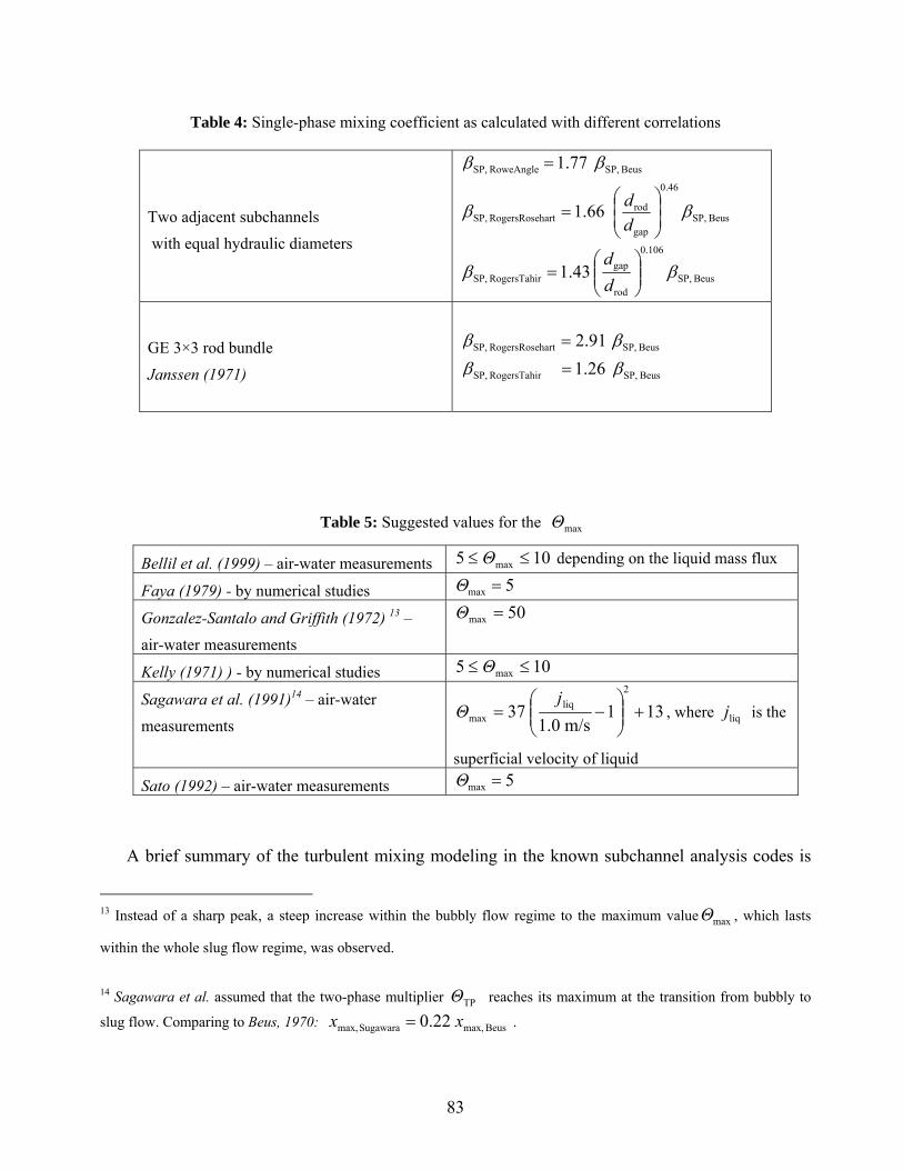
Table 4: Single-phase mixing coefficient as calculated with different correlations

Beus SP,RoweAngle SP, 77.1 ββ =

Beus SP,

46.0

gap

rodhartRogersRo SP,β se 66.1 β⎟

⎟⎠

⎞⎜⎜⎝

⎛=

dd

Two adjacent subchannels with equal hydraulic diameters

Beus SP,

106.0

rod

gap43.1 ββ ⎟⎟⎠

⎞⎜⎜⎝

⎛=

d rRogersTahi SP, d

GE 3×3 rod bundle

P

Janssen (1971)

,hartRogersRose SP, 91.2 Beus Sββ =

Beus SP,rRogersTahi SP, 26.1 ββ =

maxΘ Table 5: Suggested values for the

maxBellil et al. (1999) – air-water measurements 5 10≤≤ Θ ing on the liquid mass flux depend

Faya (1979) - by numerical studies 5max =Θ

50max =Θ Gonzale and Griffz-Santalo ith (1972) 13 – air-water measurements

Kelly (1971) ) - by numerical studies 105 max ≤≤ Θ

Sagawara et al. (1991)14 – air-water measurements

131m/s0.1

372

liq +⎟⎠

⎞⎜⎝

⎛−=

jΘ , where is the liqjmax ⎟⎜

superficial velocity of liquid

Sato (1992) – air-water measurements 5max =Θ

A brief summary of the turbulent mixing modeling in the known subchannel analysis codes is

13 In

within the whole slug flow regime, was observed.

14 Sagawara et al. assumed that the two-phase multiplier reaches its maximum at the transition from bubbly to

slug flow. Comparing to Beus, 1970:

stead of a sharp peak, a steep increase within the bubbly flow regime to the maximum value maxΘ , which lasts

TPΘ Beus max,Sugawara max, 22.0 xx = .

83

given below15. It will be seen that, excluding NASCA code, the subchannel analysis codes do not

model the spac mixing between adjacent subchannels.

1981). The l

lent mixing are given respectively as

er grids effect on the amount of turbulent

5.1.2 Turbulent Mixing Model of THERMIT-2

THERMIT-2 is a two-fluid two-phase subchannel code developed at the Massachusetts Institute

of Technology (Kelly, J. et al., ateral exchanges of mass, energy, and momentum due

to turbu dxsWW ijijkk )''(= ; ; and

F ijk

dxsqQ ijijkk )''(=

dxsijk )(τ= ngth between subchannels i and j; the is

the

heat fluxes due to turbulent m xing;

. In these equations, ijs is the gap le dx

axial mesh node size; kW '' is the phase k mass flux due to turbulent mixing; kq '' is phase k

ki τ is the phase k shear stress due to turbulent m

The turbulent shear stress term is approximated as

ixing.

( )l

GG ji −≈ε

τ where the turbulent velocity

is defined as ijsl ρ

ocity is calculated using the correlation by Rogers and Rosehart

modeled by Beus (Beus, S. G., 1970). The maximum of the two-phase multiplier is assumed equal

to 5: 5max =Θ .

Wε '

= .

The single-phase turbulent vel

(Rogers, J. T. and Rosehart, R. G., 1972). The dependence of the mixing rate on the flow regime is

5.1.3 Turbulent Mixing Model of COBRA-TF

The FLECHT_SEASET version of COBRA-TF (Paik, C.E. et al., 1985) is utilizing the same

models for turbulent mixing and void drift as the THERMIT-2 code but without applying the Beus’

15 In the following description, the nomenclature is as given in the corresponding References

84

model for the two-phase turbulent mixing.

urbulen Mixing Model of MATRA

Korea. (Yoo, Y. J. et al., 1999). In similarity to THERMIT-2 alculates the net lateral

mass flux due to turbulence as

5.1.4 T t

The subchannel code MATRA is an improved version of COBRA-IV-I developed at KAERI,

, MATRA c

GSW ijk β='' and uses the Beus’ model for the two-phase turbulent

mixing.

5.1.5 Turbulent Mixing Model of FIDAS

FIDAS is a three-fluid three-field code (Sagawara, S. et al., 1991). The code calculates the net

lateral mass flux due to turbulence as ( ) ijT

T

ijTMMij ScSc

W ρρµ

ρµρεε ∇⎟⎟

⎠

⎞⎜⎜⎝

⎛+−=∇+−= , where

cDSc

ρµ

=

is the Schmidt number. The turbulent dynamic viscosity is given as ∑ ⎟⎞

⎜⎛ +=

uulmT ρµ ,

where L is axial l h; and the mixing length is calculated

as

⎠⎝

2

zL

the lateral length; z is the engt

⎟⎟⎠

⎜⎜⎝

==2

,,1,1

jhihavehm KDKl . The single-phase turbulent velocity is calculated by Rogers and

Rosehart (Rogers, J. T. and Rosehart, R. G., 1972). The Beus’ model (Beus, S. G., 1970) is

Beus max,Sugawara max,

⎞⎛ + DD

modified such as and 22.0 xx = 131m/s0.1

2

max ⎟⎠

⎜⎝

5.1.6 Turbulent Mixin

37 liq +⎟⎞

⎜⎛

−=j

Θ .

g Model of VIPRE-2

V 2 i

We

IPRE- s a two-fluid two-phase code developed at PNL/EPRI, USA and currently used in

stinghouse, USA for safety analyses (VIPRE-02, 1994). The turbulent crossflow occurs by an

equal mass exchange between subchannels and is assumed equal to GSW mβ=' . As a second

85

option, an empirical formulation dy diffusivity t of the turbulence in terms of ed ε is employed:

⎟⎠⎝ l⎞

⎜⎛=

SW mtρε' , where is the gap width, is the gap centroid length, S l G is the average mass

flux in the lateral control volume, mρ is the mixture density, ⎟⎠

⎜⎝

=lU m

m⎞⎛t 1ε

β is an empirical mixing

coefficient, and is the mixture axial velocity. The turbulenmU t energy exchange in the lateral

direction for each phase is e phase mass fraction, and it is computed using the

relation

weighted by th

∑ ∆∆−=ik m

t hWXQε

φφφ

φ ρ

ρα ' , where X∆ is the axial node l i

difference across the lateral control volume for phase

ength, ∆ s the enthalpy φh

φ , and ∑ik ε

is a summation over all gaps k

onnected to channel i. The turbulent mixing between channels is included as a force in the axial

momentum equation. The total axial force, , in each phase due to turbulent momentum mixing is

computed as

c

mF

∑ ∆∆−=ik m

Tm UWXCFε

φφφ

ρ

ρα ' , where φU∆ is the axial velocity difference for phase

across the lateral control volume. The term is an empirical correction factor (the so called

turbulent momentum factor) to account for the imperfect analogy between turbulent transport of

thermal energy and momentum. If

TC

0.1=TC , energy and momentum are mixed with equal strength.

If , only energy is mixed by the turbulent crossflow. Turbulent momentum exchange is not

c

The development of the NASCA code is a joint work of several academic and industrial

organizations in Japan (Ninokata, H. et al., 2001, Hotta, A. et al., 2004, and Shirai, H. et al., 2004).

0.0=TC

onsidered in lateral direction.

5.1.7 Turbulent Mixing Model of NASCA

86

( ) ( ){ }jkkikkTMTP

TMkij lραραεTurbulent mixing is modeled as φ −⎟

⎠⎞

⎜⎝⎛=

,, , where the two-phase turbulent

velocity is given as ⎟⎟⎠

⎞⎜⎜⎝

⎛⎟⎠⎞

⎜⎝⎛=⎟

⎠⎞

⎜⎝⎛

TP

kTM

SPTMTP ll ρρ

θεε

,

xing velocity on the geometry. The geom

. NASCA assumes a dependence of the single-

phase mi etry effect is modeled by applying the so-called

rod shape factor *iF , which accounts for the spacer grids as well:

10

**

1(1

111

−

−

⎞

⎜⎜

⎛

=⎟⎞

⎜⎛

+==⎟⎞

⎜⎛

y

yji

j

iSFFε 0

1)()−

⎟⎟⎟⎟⎟

⎠⎜⎜

⎜

+⎟⎠

⎜⎝+⎠⎝

∫∫

jiijjiijkjkiSP

dyyS

dyy

SSlll εεεε, where is the gap size

at the lateral distance (see Figure 7).

⎝kjki εε

)(yS

i j

y=0y=yi

S(y)

i j

y=0y=yi

S(y)

Figure 7: Definition of the gap size at the lateral distance in NASCA

MONA-3 is a three-field two-phase code developed in Westinghouse, Sweden in cooperation

5.1.8 Turbulent Mixing Model of MONA-3

with Studsvik Scandpower AS and the Royal Institute of Technology, Stockholm (Nordsveen, M. et

al., 2003). The effect of turbulent mixing is modeled for momentum and energy equations. A

turbulent viscosity concept is used and both a Prandtlt type model and a model by Ingesson

87

(Inges , 1son, L. 969) are implemented:

2)(2 kjkik

mU

lij

Tk lνν

ν =+

+∆ ,

ijgap

ijgapm

ldl

ld +

⋅= Prandtl type

820kk

Tkν Υ= , 2.0Re18.0 −= kf , Re fν

hD12.6=Υ Ingesson’s model

n the above equations, l is the mixing length; d is the gap width, U

P

I m gap k∆ is the phase velocity

difference between the two subchannels; Υ is the velocity adjustment factor; and is the distance

between the centers of gravity of the subchannels.

5.2 ing Model

In the COBRA/TRAC code version, only a single-phase mixing (single-phase liquid for void

fractions below value of 0.6, single-phase vapor for void fractions above value of 0.8, and a ramp

bet f the traditional mixing coefficient approach. Later,

in the FLECHT SEASET code version, a void drift model based on the work of Lahey and Moody

(Lahey, R. T. and Moody, F. J., 1993

ass ous phase and its modeling has been not applied to the

hot wall flow regimes. However, the model implementation into the COBRA-TF conservation

equations led to a distortion of th

conditions. As discussed in section 3.3.3, F-COBRA-TF modeling of turbulent mixing and void

drift was revised and improved by Avramova (Avramova, M. N., 2003b). The following sections

wil

ijl

F-COBRA-TF Turbulent Mix

ween the two) has been modeled by means o

) has been employed (see section 3.3.3). Void drift was only

umed to occur when the liquid is continu

e mass balance and numerical instabilities at pre- and post-CHF

l describe the current code models for intra - and intersubchannel mass, momentum, and energy

transfer.

88

5.2.1 F-COBRA-TF Turbulent Mixing and Void Drift Models

The F-COBRA-TF turbulent mixing and void drift models assume that the net two-phase

mix void fraction gradient. At an

annular film flow regim assumed and only the turbulent mixing of vapor and

entrained droplets is modeled. In other words, the void drift is only modeled in bubbly, slug, and

churn flow, where liquid is the continuous phas

2005b).

The lateral exchange due to turbulent mixing

ing (including void drift) is proportional to the non-equilibrium

e a void drift offset is

e and vapor is the dispersed phase (Glueck, M.,

is modeled as follows:

Turbulent mixing of mass in phase k:

(TM GAGm )( ραβραβ =∆−=& )iijjk k,k,k,k,kk ραρρ

− (5.12)

Turbulent mixing of momentum in phase k:

AGGI TMk k∆−= β& (5.13)

ρ

Turbulent mixing of energy in phase k:

AhGTM ραρ

β ∆−=&

In Equations 5.12 through 5.14 SPTP

Qk )( kkk (5.14)

ββ Θ= is the two-phase turbulent mixing coefficient.

Currently the single phase mixing coefficient SPβ may be either specified as a single input value

or internally calculated choosing between two empirical correlations: Rogers and Rozehart (Rogers,

J. T. and Rosehart, R. G., 1972) and Rogers and Tahir (Rogers, J. T. and Tahir, A. E. E., 1975). The

89

two-phase mul se

turbulent mixin

tiplier TPΘ is calculated using the Beus’ approach (Beus, S. G., 1970) for two-pha

g as given by Equations 5.8 through 5.11.

The lateral exchange due to void drift is modeled as follows:

Mass exchange in phase k by void drift:

( ) AGm iijjVD

EQ,k,EQ,k,EQ,k,EQ,k, ραραβ −=& (5.15)

Momentum exchange in phase k by void drift:

k ρ

( ) AGGGI ijVDk EQ,k,EQ,k, −=

ρβ& (5.16)

Energy exchange in phase k by void drift:

( ) AhhGQ iiijjjVDk EQ,k,EQ,k,EQ,k,EQ,k,EQ,k,EQ,k, ραρα

ρβ −=& (5.17)

According to Levy (Levy, S., 1963) the equilibrium density distribution is related to the mass

ux distribution. This assumption was further used by Drew and Lahey (Drew, D. A. and Lahey, R.

ical derivation of a void drift model for subchannel analyses. The model is well

documented and currently used in many subchannel codes. Detailed description of the

implementaion of the Drew and Lahey’s model in the THERMIT-2 (MIT) and the COBRA-TF

(PSU) subchannel codes are published in Kelly, J. E. et al., 1981 and Avramova, M. N., 2003b. The

model is used in F-COBRA-TF as well.

fl

T., 1979) for analyt

90

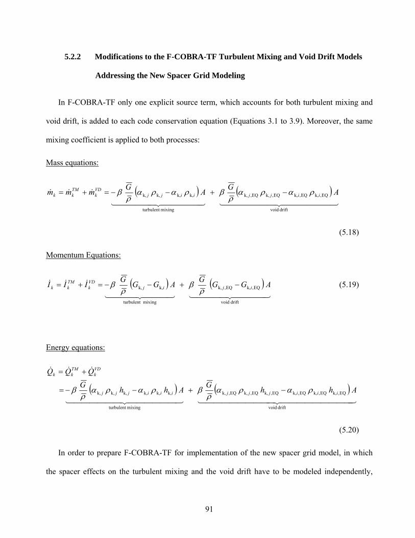
5.2.2 Modifications to the F-COBRA-TF Turbulent Mixing and Void Drift Models

Addressing the New Spacer Grid Modeling

In F-COBRA-TF only one explicit source term, which accounts for both turbulent mixing and

void drift, is added to each code conservation equation (Equations 3.1 to 3.9). Moreover, the same

mixing coefficient is applied to both processes:

Mass equations:

( ) ( )444444 2144444 344444 21EQ,k,EQ,k,k,k,k,k, ijiijjkkk ρρ 4444 344

&&&

drift void

EQ,k,EQ,k,

mixingturbulent

AGAGmmm ijVDTM ραραβραραβ −+−−=+=

(5.18)

Momentum Equations:

( ) ( )4444 34444 21444 3444 21

&&&

driftvoid

EQ,k,EQ,k,

mixingturbulent

k,k, AGGGAGGGIII ijijVDk

TMkk −+−−=+=

ρβ

ρβ (5.19)

Energy equations:

( ) ( )EQ,k,EQ,k,EQ,k,EQ,k,EQ,k,EQ,k, AhhA iiijjji ραραρ

β −+ 444444444 3444444444 21444444 3444444 21

&

drift voidmixingturbulent

k,k,k,k,k,k, GhhGQQQ

iijjj

kkk

ραραρ

β −−=

+=

In order to prepare F-COBRA-TF for implementation of the new spacer grid model, in which

the spacer effects on the turbulent mixing and the void drift have to be modeled independently,

&& VDTM

(5.20)

91

minor coding modifications were performed such that at tw

phase multipliers are applied to the turbulent mixing and to the void drift terms: the two-phase

turbulent mixing multiplier and the void drift multiplier Θ

to the mass conservation equation of phase k is given as:

o-phase conditions two different two-

TMTPΘ VD

TP . Then, for example, the source

( ) ( )44444444 344444444 21444444 3444444 21

drift voidmixingturbulent

VDTM +=

&&&

EQ,k,EQ,k,EQ,k,EQ,k,k,k,k,k, AGAGmmm

iijjSPVDTPiijjSPTP

k

ραραρ

βραραρ

β −Θ+−Θ−=

+=

(5.21)

Moreover, instead of introducing one combined source term kkk mmm &&& to the right hand

side (RHS) of the phase k mass equation, two independent terms and are evaluated and

added:

TM

VDTMkk

TMkm& VD

km&

( ) AGm iijjSPTMTP

TMk k,k,k,k, ραραβ −Θ−=& (5.22)

ρ

and

( ) AGiijjSP

VDk EQ,k,EQ,k,EQ,k,EQ,k, ραρα

ρβ −Θ= (5.23m VD

TP& )

In similarity, sources to the phase k momentum equation are

( ) AGGI ijSPTMTP

TMk k,k, −−=

ρβ& (5.24) G

Θ

( ) AGGI ijSPVDTP

VDk EQ,k,EQ,k, −Θ=

ρβ& (5.25)

k

G

and sources to the phase energy equation are

92

( ) AhhGQ TMTM ραραρ

β −Θ−=& (5.26) iiijjjSPTPk k,k,k,k,k,k,

( ) AhhGQ VDVD ραραρ

β −Θ=& (5.27)

In the above equations, superscripts TM and VD stand for turbulent mixing and void drift,

respectively.

It c

iiijjjSPTPk EQ,k,EQ,k,EQ,k,EQ,k,EQ,k,EQ,k,

an be seen that the major assumption of the turbulent mixing modeling is not changed: the

same single-phase mixing coefficient SPβ is applied to the ma momentum, and energy exchange: ss,

UyCt=β , where == tttt : aDCSP ∆

= ν .

A sensitivity study confirmed that the new coding approach does not create numerical

instabilities since the net amount of mass, momentum, and energy added to the RHS of the

conservation equations have not changed.

5.2.3 Modifications to F-COBRA-TF Turbulent Mixing and Void Drift Models

Addressing Some Experimental Findings

During the Kumamoto University air-water experiments it has been found that the two-phase

multiplier , which corrects the single-phase mixing coefficient, has different dependence on the

void fraction for fully-developed and for developing flows, as it is shown in Figure 8 and Figure 9.

Ba ation, the authors of NASCA code (Hotta, A., 2005) have applied two different

two-phase m ltipliers: turbulent mixing two-phase multiplier

TPΘ

sed in this observ

u TMΘ and void drift multiplier VDΘ .

The Kumamoto University experimental observations were modeled in F-COBRA-TF. In F-

93

COBRA-TF, the transition to annular flow is not necessary controlled by a fix void fraction value,

therefore to be in an agreement with the code flow regime logic, the void drift coefficient was

disabled in annular flow. The code modification was validated against 4×4 PELCO-S experiments

(Herkenrath, H. et al., 1979). Because the F-COBRA-TF comparisons showed that the

implementation of the Kumamoto University model into F-COBRA-TF leads to significant

misprediction of the measured distribution of the exit quality, the model was removed from the

code.

In addition, the equilibrium distribution weighting factor , was correlated to the pressure as

proposed by KAERI (Jeong, J. J. et al., 2005b):

MK

[ ]PK 215.0exp2.6M −= .

94

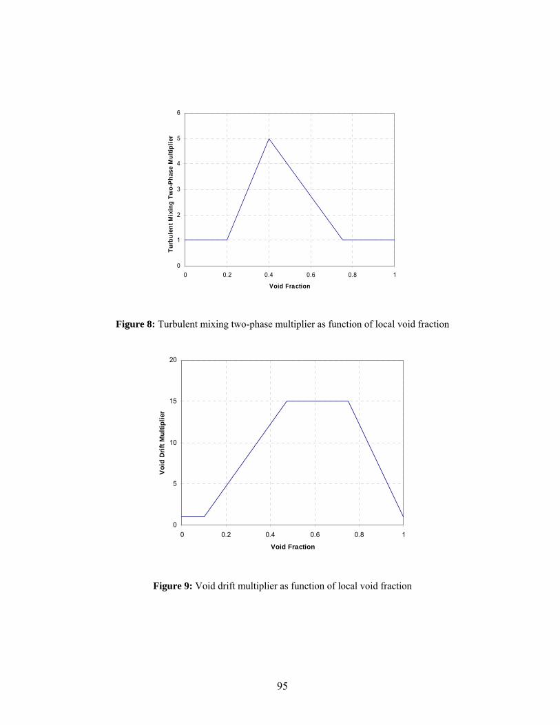
5

iplie

r

0

1

2

3

4

0 0.2 0.4 0.6 0.8 1

Turb

ent M

ing

Tw

hase

6

Void Fraction

ulxi

o-P

Mul

t

Figure 8: Turbulent mixing two-phase multiplier as function of local void fraction

20

00 0.2 0.4 0.6 0.8 1

5

10

15

Void Fraction

Voi

d Dr

ift M

ultip

lier

Figure 9: Void drift multiplier as function of local void fraction

95

5.3 Evaluation of the Single-Phase Mixing Coefficient by Means of CFD

Calculations

5.3.1 Methodology

omputatC ional fluid dynamics can be utilized for an evaluation of the single-phase mixing

coe

Approach 1: Evaluation of the single phase mixing coefficient by the turbulent viscosity

fficient in two ways: 1) by CFD predictions of the turbulent viscosity (Ikeno, T., 2001) or 2) by

CFD predictions of the turbulent heat flux across the gap between adjacent subchannels (Jeong, H.

et al., 2004). In both methods, the CFD model must be settled correctly to assure the diffusive

nature of the turbulent mixing processes: no net mass flow over the gaps between subchannels must

occur.

Let’s assume two identical subchannels connected through a gap (Figure 10).

According to Equation 5.4 the dimensionless turb xing coefficient

Figure 10: Model for the evaluation of the single-phase mixing coefficient by the turbulent viscosity

ulent mi β can be defined by

applying kinematical turbulent viscosity as a turbulent diffusion coefficient ( turbtC ν≡ ):

Uyturb

SP ∆=ν

β , (

wh

5.28)

ere turbν is the surface-averaged kinematical turbulent viscosity, U is the surface-averaged

y∆

96

vertical velocity, and is the centroid distance bey∆ tween adjacent subchannels. Both, turbν and U

can be evaluated from single-phase CFD calculations.

Approach 2: Evaluation of the single phase mixing coefficient by the turbulent heat flux across

the gap

Let us assume two adjacent subchannels with identical geometries and equal inlet mass

velocities (Figure 11). A temp

subchannel j (right ld

one. Thus, the heat transfer between both subchannels is achieved only by two processes –

conduction and turbulent diffusion (mixing).

Figure 11: Model for evaluation of the single-phase mixing coefficient by the turbulent heat flux across

The heat rate due to turbulent mixing and conduction per unit length through the gap Sij (at

stea state flow conditio

. (5.29)

The heat flux through the gap is given as:

erature difference of 10 °C between the subchannels is applied. The

i (left side) is assumed to be the hot one, while the subchannel side) is the co

the gap

dy ns) is equal to

xSqQQQ ijtotalini

outitotal ∆=−= ''

∆x

∆y

iniQ

injQ

out outQiQ j

hot cold Sij

97

( )443442143421

&

&ii h

ini

outip

m

flowiiiiiijtotal TTcAUhmxSq

∆

−=∆=∆ ρ'' (5.30)

( ) ''''''in

iout

ipflow

iii qqTTcAU

q +=−

=ρ

conductionturbulencetotal xS ∆ (5.31)

The he

ij

at flux through the gap due to conduction is:

( )yTT

qout

ioutj −

−= λ'' . (5.32) conduction ∆

The heat flux through the gap due to turbulent mixing is:

( ) ( )⎟⎜ ∆∆ yxSconductiontotalturbulence

ined as:

⎟⎠

⎞⎜⎝

⎛ −−−

−=−=

TTTTcAUqqq

outi

outj

ij

ini

outip

flowiii λ

ρ'''''' . (5.33)

Thus, the turbulent mixing coefficient can be def

fluxheat axiale turbulenc todueflux heat t coe mixing p se-ingle fficienhas =

or (5.34)

)(

''

ijp

turbulence

TTUcq

−=

ρβ .

Since, for water the turbulent thermal conductivity is much higher than the molecular one

Equation 5.34 can be written as:

)(

''

ijp TTUc −=

ρβ (5.35)

turbulencetotal

totalq

where qq ≡ . ''''

98

In theory, when the mixing coefficient is defined using Equation 5.28 it will be representing

only turbulent diffusion, but not molecular diffusion. On other hand, Equation 5.35 will calculate

the mixing coefficient due to turbulent and molecular diffusion together.

Here, it should be highlighted that the heat flux determined by a subchannel based heat balance

( inout TT − ) will inii clude the contribution of both convective and diffusive transfers. The real

diff only by a local (near gap) heat balance

ogT

In regard to F-COBRA-TF, since the code is developed for LWR applications both

methodologies are applicable, but the one using heat transfer balance seems to be more appropriate

for the scale of subchannel analyses. However, both approaches were examined and compared in

regard to their applicability and numerical stability.

5.3.2 CFD Model

For purpose of preliminary investigations of the proposed methodology for the single-phase

ation, a simple 2×1 STAR-CD (STAR-CD Version 3.26) model for thermal-

hydraulic analyses of the heat transfer between adjacent subchannels has been developed at

AREVA NP GmbH (Kappes, Ch., 2006). The model corresponds to ones shown in Figure 10 and

Figure 11 and it simulates only a heat transfer by diffusive effects. No net mass transfer is assumed

to occur. The objective was to study the turbulence in the gap between the rods. Segments of six

rods with outer diameters of 9.5 mm were arranged in a 2×1 subchannels configuration with a rod-

to-rod pitch of 12.7 mm over the axial length of 540 mm. The coupled subchannels have equal inlet

velocities, but the inlet temperatures differ by 10 °C. The applied boundary conditions are inlet

velocity of 5 m/s and outlet pressure of 160 bars; symmetry condition is assumed at the gaps

usive heat flux over the gap region can be evaluated

( ingap

utap T− ).

mixing coefficient evalu

99

between the ity of 5 %

is modeled. The water properties are assumed to remain constant along the axial length. A simple

conjugated-gradient solver with upwind discretization was used. The standard

rods; the walls are smooth, no-slip, and adiabatic. The inlet turbulence intens

ε−k high Reynolds

number turbulence model was utilized. The accuracy was set to 10-4 and typical mesh size of 0.3

mm was selected.

The 2×1 STAR-CD model is summarized in Table 6.

In total ten sub-models were calculated. At the beginning no internal structures were included: a

clean bundle was simulated. In the next four models straps with different thicknesses were inserted,

respectively 0.3 mm, 0.4 mm, 0.5 mm, and 0.6 mm. In the last set of calculations, the model with

strip thickness of 0.4 mm was selected and four mixing vanes were attached at the upper edge of the

strip. The vane angle was varied between 10 and 50 degrees in intervals of 10 degrees. The mixing

vanes were mirrored and rotated in order to produces pure circular flow inside the subchannels.

The model and the mixing vanes configuration are visualized in Figure 12 and Figure 13,

respectively. Figure 14 shows the mesh structure of the model. The mixing vane geometry is given

in Figure 15.

The distributions of the temperature field, turbulent viscosity, vertical velocity, and pressure

field are given in Table A-1through Table A-8 of Appendix A.

100

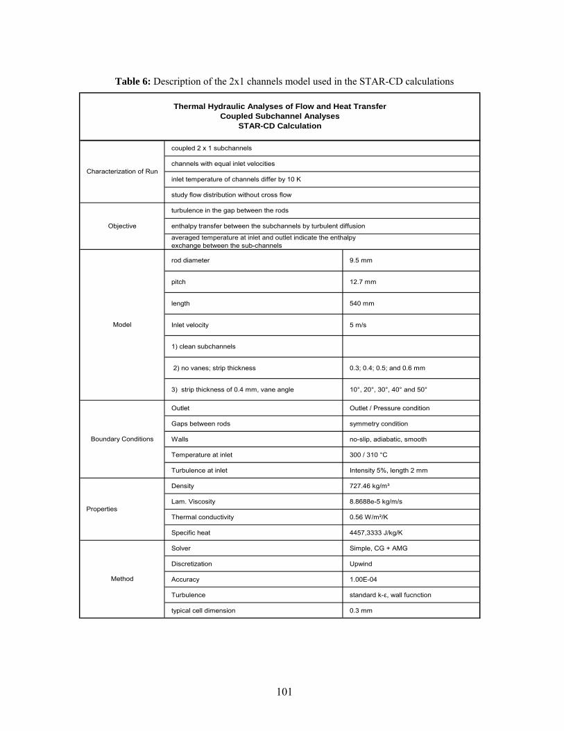
Table 6: Description of the 2x1 channels model used in the STAR-CD calculations

ion

typical cell dimension 0.3 mm

inlet temperature of channels differ by 10 K

Properties

Model

Objective

Boundary Conditions

Method

Thermal Hydraulic Analyses of Flow and Heat TransferCoupled Subchannel Analyses

STAR-CD Calculation

study flow distribution without cross flow

turbulence in the gap between the rods

enthalpy transfer between the subchannels by turbulent diffusion

averaged temperature at inlet and outlet indicate the enthalpy exchange between the sub-channels

Characterization of Run

coupled 2 x 1 subchannels

channels with equal inlet velocities

rod diameter 9.5 mm

pitch 12.7 mm

length 540 mm

Inlet velocity 5 m/s

1) clean subchannels

2) no vanes; strip thickness 0.3; 0.4; 0.5; and 0.6 mm

3) strip thickness of 0.4 mm, vane angle 10°, 20°, 30°, 40° and 50°

Outlet Outlet / Pressure condition

Gaps between rods symmetry condition

Walls no-slip, adiabatic, smooth

Temperature at inlet 300 / 310 °C

Turbulence at inlet Intensity 5%, length 2 mm

Density 727.46 kg/m³

Lam. Viscosity 8.8688e-5 kg/m/s

Thermal conductivity 0.56 W/m²/K

Specific heat 4457,3333 J/kg/K

Solver Simple, CG + AMG

Discretization Upwind

Accuracy 1.00E-04

Turbulence standard k-ε, wall fucnct

101

Figure 12: 2×1 CAD model nsfer by turbulent diffusion

for thermal-hydraulic analysis of heat tra

Figure 13: Side and top views of the mixing vanes configuration

102

Figure 14: Mesh grid of the 2×1 model

Figure 15: Geometrical characteristics of the mixing vanes in the 2×1 model

103

5.3.3 Evaluation of the Single-Phase Turbulent Mixing Coefficient

-model the following data was extracted from the CFD results:

i j

2) Axial distribution of the surface-averaged dynamic turbulent viscosity surfturbµ ;

3) Axial distribution of the subchannels gap-averaged temperatures gapiT and gap

jT ;

4) Axial distribution of the subch

Using the results obtained with the above described 2×1 STAR-CD model, the single-phase

mixing coefficient was evaluated with both approaches discussed in section 5.2.1 (Equations 5.32

and 5.34). For each sub

1) Axial distribution of the subchannels surface-averaged temperatures T and T ;

annels gap-averaged dynamic viscosities and ;

tan

surf surf

gapiturb,µ gap

jturb,µ

5) Axial distribution of the subchannels gap-averaged vertical velocities gap and gap

The surface-averaging is done over each subchannel cross-sectional area at every 10 mm axial

elevation and the gap-averaging is done over shells of -0.1 mm (left side – subchannel i ) and 0.1

mm (right side – subchannel j ) from the gap between subchannels at every 10 mm axial elevation.

The data is available also in a fine axial scale of 3 mm. Because of the assumption for cons t

water properties, the surface-averaged axial velocity,

iU jU .

surfU , is equal to the inlet vertical velocity of

5 m/s over the whole length.

During the investigation of the single-phase mixing coefficient by a heat balance, it was found

that a smother axial distribution of the heat flux across the gap is evaluated when instead of taking

the heat balance over a subchannel control volume, the balance is performed with a local

temperature gradient over the gap.

Figure 17 through Figure 22 show the axial behavior of the evaluated single-phase mixing

104

coefficients for different strap thickness and vane declination angles. For the purpose of

comparative analyses, the evaluations with Approach 1 were performed in two ways: 1) using

surface-averaged quantities - surf

surfturb

SP =ν

β ; and 2) using gap-averaged quantities - Uy∆

gapturb

SPUy∆

=ν

β . It can be seen in Figure 17 and Figure 18 than for the cases with no mixing vanes gap

both methods predict relatively close axial distributions of the mixing coefficient: there is a sharp

increase downstream of the strap upper edge followed by a decrease, after which a tendency exists

of stabilizing around the clean bundle value. The mixing coefficient calculated by surface-averaged

qua

The picture becomes more complicated and somehow difficult to explain when the mixing

vanes are added - Figure 19 and Figure 20. Physically, due to the swirl flow created by the mixing

vanes, the turbulence downstream of the vanes is expected to be significantly enhanced. However,

this phenomenon is not captured by our evaluations of the mixing coefficient by using turbulent

viscosity. In completely opposite manner, Figure 19 indicates a decrease of the mixing coefficient.

This unexpected result is not due to errors during the extractions of the CFD data or during the

ntities tends to be a little bit higher.

SPβ

evaluations, because it is in an agreement with the turbulent viscosity distributions over subchannel

cen

When evaluating the single-phase mixing coefficient

troids line as given in Table A-8 of Appendix A.

SPβ by the turbulent viscosity and the

vertical velocity averaged over the gap region (see Figure 20) there is an increase in the mixing rate,

ixing

vanes. After that region the turbulence tends to reach the clean bundle values. Again, these

predictions are following the turbulent viscosity distributions over gap between rods as given in

but upstream of the mixing vanes and a sharp decrease exists over and shortly after the m

105

Table A-8 of Appendix A.

Other important observation is that the magnitude of the mixing coefficients evaluated with

Approach 1 is one order lower than the expected value of 10-3 for the simulated conditions. Let’s

recall that our CFD calculations were performed with the standard ε−k turbulence model. This

model neglects the large eddy structures, which exist in the gap region and have a significant

contribution to the exchange processes between subchannels by their cyclic flow pulsation through

the gaps. As already discussed in section 2.3 the same finding were reported by Ikeno (Ikeno,T.,

2001).

From analyses of the evaluated mixing coefficients by the heat transfer balance (Approach 2,

see Figu lly

reasonable results. Right after the straps there is an augmentation in the turbulent mixing due to

flow

e 22) - a decrease in the turbulent mixing is

obs

ed model of Ikeno (Ikeno,T., 2001) (see Figure 16). As described in section 2.3,

Ike

re 21 and Figure 22) it can be stated that this method results in more stable and physica

area expansion. Thicker the strap is, stronger the mixing is. An interesting behavior is found

shortly downstream of the mixing vanes (see Figur

erved in that region. After that the turbulence quickly recovers and lasts up to the next strap. The

length of the decrease depends on the declination angle – larger the declination angle is, shorter the

decrease is. Higher mixing coefficient corresponds to larger vane angle.

It should be mentioned here that the short decrease right downstream of the vanes has been seen

also in the improv

no overcame the deficiency of the standard ε−k turbulence model to capture the large eddy

structure at the gap region by adopting the flow pulsation model of Kim and Park (Kim, S., and

Park, G.-S., 1997) with analytical formula for the Strouhal number.

106

107

Figure 16: The non-dimensional eddy thermal diffusivity calculated by Ikeno (Ikeno,T., 2001

Another important advantage that Approach 2 shows is the magnitude of the evaluated mixing

coefficients – they are in the expected range of 10-3.

The above discussed investigations of the proposed methodologies for evaluation of the single-

phase mixing coefficient by means of CDF calculations led to the selection of the so-called

Approach 2: Evaluation of the single-phase mixing coefficient by the turbulent heat flux across the

gap for an implementation into F-COBRA-TF for modeling of the enhanced turbulent mixing by

the spacer grids.

The selected method was used for estimations of the spacer mixing coefficient for the

ULTRAFLOWTM spacer design (trademark of AREVA NP GmbH). Comparative analyses to the

original F-COBRA-TF spacer grid modeling were performed for the ATRIUMTM10 XP BWR

bu e

measurements does not allowed a validation of the proposed method against experimental data.

)

ndle, with is equipped with ULTRAFLOWTM spacers. The lack of suitable AREVA NP in-hous

Single-Phase Mixing Coefficientsurface-averaged

0.0000

0.0002

0.0004

0.0006

0.0008

0 100 200 300 400 500 600

Height, mm

Mix

ing

coef

ficie

nt 0.3 mm0.4 mm0.5 mm0.6 mmclean channels

strip

valuation of the single-phase mixing coefficient using surface-averaged turbulent viFigure 17: E scosity and

vertical velocity – dependence on the strap thickness

Single-Phase Mixing Coefficientgap-averaged

0.0000

0.0001

0.0002

0.0003

0.0004

0.0005

0 100 200 300 400 500 600

Height, mm

Mix

ing

coef

ficie

nt 0.3 mm0.4 mm0.5 mm0.6 mmclean channels

strip

Figure 18: Evaluation of the single-phase mixing coefficient using gap-averaged turbulent viscosity and

vertical velocity – dependence on the strap thickness

108

Single-Phase Mixing Coefficientsurface-averaged

0.0000

0.0002

0.0004

0.0006

0.0008

0 100 200 300 400 500 600

Height, mm

Mix

ing

coef

ficie

nt 10 deg20 deg50 degno vanesclean channels

strip

Figure 19: Evaluation of the single-phase mixing coefficient using surface-averaged turbulent viscosity and

vertical velocity – dependence on the declination angle (strap thickness of 0.4 mm)

Single-Phase Mixing Coefficientgap-averaged

0.0000

0.0001

0.0002

0.0003

0.0004

0.0005

0 100 200 300 400 500 600

Height, mm

Mix

ing

coef

ficie

nt 10 deg20 deg50 degno vanesclean channels

strip

Fig nd vertical v .4 mm)

ure 20: Evaluation of the single-phase mixing coefficient using gap-averaged turbulent viscosity aelocity – dependence on the declination angle (strap thickness of 0

109

Single-Phase Mixing Coefficient

0.0000

0.0005

0.0010

0.0020M

ixi

coe

ffien

t

0.0015

0 100 200 300 400 500 600

Height, mm

ngci

clean channels

strip

0.3 mm0.4 mm0.5 mm0.6 mm

Figure 21: Evaluation of the single-phase mixing coefficient by local heat balance over the gap – dependence on the strap thickness

Single-Phase Mixing Coefficient

0.0000

0.0005

0.0010

0.0015

0.0020

0.0025

0 100 200 300 400 500 600

Height, mm

Mix

ing

coef

ficie

nt

10 deg20 deg30 deg50 degno vanesclean channels

strip

Figure 2 e gap – dependence on the declination angle (strap thickness of 0.4 mm)

2: Evaluation of the single-phase mixing coefficient by local heat balance over th

110

5.3.4 Incorporation of the CFD Results into F-COBRA-TF

The effect of the spacer grids on the turbulent m

, which is applied to the turbulent mixing rate as their are calculated by the current F-COBRA-

odels. The multiplier is a ratio of the

with mixing type spacer grid, , and the single-phase mixing coefficient evaluated for a

“clean” bundle, . It is a function of the axial dist

mixing vanes angle

ixing is modeled by an additional multiplier,

TMSGΘ

TF m single-phase mixing coefficient evaluated for a bundle

spacersSPβ

spacersnoSPβ ance y downstream of spacer and the

ϕ :

spacersnoSP

spacersSPTM y

ββϕ =Θ ),(

. (5.36)

It was expected that the spacer multiplier will have a peak near the upper edge of the mixing

vanes and will decrease further downstream. Its magnitude will increase with the strap thickness

(following the magnitude of the change in the flow area) and with the declination angle of the vanes

(following the magnitude of the swirling flow). Schematically, this behavior is shown in

Figure 23.

SG

1.0

TMSGΘ

x ZSG,1 ZSG,2 … ZSG,N

φ 1 > φ 2 ----- φ2 ___ φ

1

Figure 23: Schematic of the spacer multiplier distribution over the axial length

111

T uahus, Eq tions (5.29); (5.31); and (5.33) were modified as follows:

( ) AGm TMTMTM ραραρ

β −ΘΘ−=& (5.37) iijjSPTPSGk k,k,k,k,

( ) AGGGI TMTMTM −ΘΘ−=ρ

β& (5.38) ijSPTPSGk k,k,

( ) AhhGQ TMTMTM ραραβ −ΘΘ−=& (5.39)

If the new spacer model is being developed to use correlations for the spacer multiplier, this will

require an extensive set of numerical experiments in order to cover a large envelope of operational

conditions. However, in the view of the F-CO

iiijjjSPTPSGk k,k,k,k,k,k,ρ

BRA-TF development for industrial applications,

instead of implementing such correlations it will be more efficient to develop an interface module

to be applied to the code turbulent mixing model. The module will: 1) contain data base with

detailed information for the spacer multiplier distributio

mixing vane designs (obtained by means of CFD calculations) and 2) will maintain the exchange

between the CFD data base and F-COBRA

code could be supplied with sets of CFD data, which represent spacer designs that are currently

used. The users will be able to choose which data set to be used. I

“ex

ulent mixing modeling and examples for the CFD obtained

data sets of the mixing multipliers are given in Appendix C.

To address the flow regime dependence of the mixing coefficient, the axial velocity used in the

CFD pre-calculations (Eq. 5.35) must be calibrated to the actual axial flow velocity of the given F-

COBRA-TF computational cell.

n across a given bundle for a set of different

-TF. For the purposes of routine safety analyses, the

n case of new design studies, an

perienced” user will create a new data set based on recent CFD calculations.

The flow chart of the enhanced turb

112

5.3.5 Evaluations of the Spacer Grid Void Drift Multiplier

words must be aid for theHere, a few s spacer effect on the void drift phenomenon. The void

drift h velocity regions. On the other hand, the spacers

are

is characterized by the vapor affinity for hig

known to change the main velocity profile because of the flow area contraction and expansion

near their locations and/or flow deflection on their surfaces. The extent of this change could be used

as a criterion for an enhancement or a suppression of the local void drift. In similarity to the spacer

grid turbulent mixing multiplier, a spacer grid void drift multiplier, VDSGΘ , could be defined by

means of CFD predictions for the change in the main velocity profile at the spacer locations. The

purpose of applying a spacer grid void drift multiplier will be to drive more vapor into the

subchannel with the higher main flow velocity.

Thus, Equations (5.30), (5.32), and (5.34) can be modified as follows:

( ) AGm iijjSPVDTP

VDSG

VDk EQ,k,EQ,k,EQ,k,EQ,k, ραρα

ρβ −ΘΘ=& (5.40)

( ) AGGGI ijSPVDTP

VDSG

VDk EQ,k,EQ,k, −ΘΘ=

ρβ& (5.41)

( ) AhhGQ iiijjjSPVDTP

VDSG

VDk EQ,k,EQ,k,EQ,k,EQ,k,EQ,k,EQ,k, ραρα

ρβ −ΘΘ=& (5.42)

However, there is yet no clear concept how exactly the applied spacer grid void drift coefficient

will be calibrated to the main velocity.

113

5.3.6 F-COBRA-TF Modeling of the Turbulent Mixing Enhancement for

ULTRAFLOWTM Spacers

5.3.6.1 ULTRAFLOWTM Spacer Design

The ULTRAFLOWTM spacer design has swirl type mixing vanes intended to generate intensive

intra-subchannel swirl and turbulence, but no net mass crossflow. In each pair of adjacent

subchannels the swirling flows have opposite directions. A 3D view of the ULTRAFLOWTM spacer

is given in Figure 24. The spacer includes four swirl deflectors attached at the upper edge of the

interconnections between the straps. The swirl deflectors have an air vane structure including blades

that are conf as a pair of

tersecting triangular base plates extending upward from the interconnecting strips. The swirl

anes are bent in the same direction from the associated side base plates. A schematic of the mixing

vanes m i Figure 25.

igured to have the same vane rotation direction. Each swirl vane h

in

v

arrange ent in a 2×2 subchannels array s shown in

Figure 24: 3D view of the ULTRAFLOWTM spacer

114

115

Figure 25: Mixing vanes configuration of the ULTRAFLOWTM spacer design

5.3.6.2 CFD Model of ULRTAFLOWTM Spacer

An existing geometrical model of ULTRAFLOWTM spacer, developed at AREVA NP GmbH

for STAR-CD 3.26, was utilized for the evaluation of the mixing coefficient by heat balance across

the gap between adjacent subchannels. A schematic of the model is shown in Figure 26.

Figure 26: Schematic of the CFD model for the ULTRAFLOWTM spacer

Center of the control volume at altitude z - used for

differences between adjacent evaluation of the temperature

subchannels

Surface of the control volume at altitude z ±15 mm - used for cross-sectional averages

An existing coordinate system from the ULTRAFLOWTM spacer model was chosen. It starts at

7.45− mm and ends at 455.8 mm. For our evaluations, the region between 40− to +440 mm was

selected. Then, the leading edge of the spacer is on the coordinate z = -5.738 mm. The top of the

vanes is at z = +23.142 mm. Since the axial spacing for the evaluation is 30 mm, the first axial

section, -40 to -10 mm, is completely upstream the spacer; the second axial section, -10 to +20

mm, is almost completely containing the spacer; the third axial section, +20 to +50 mm, is almost

completely downstream the spacer (only the first 3mm contain a part of the top of the vanes); and

the fourth and following axial sections are in the region of the undistorted geometry of the bare rod

bundle.

The CFD analyses were all conducted with an inlet velocity of 2.59 m/s. The coupled

subchannels have equal inlet velocities, but different inlet temperatures. The water properties are

assumed to remain constant. A simple conjugated-gradient solver with upwind discretization was

used. The standard ε−k high Reynolds number turbulence model was utilized. The convergence

was set to 10-4.

CFD calculations were performed for two cases: 1) simulation of one span of a real

ULTRAFLOWTM spacer and 2) simulation of a “clean” 2×1 array of the ATRIUMTM10 XP bundle.

The distributions of the velocity and temperature fields and the turbulent viscosity are given in

Table B-1 through Table B-3 of Appendix B. The axial distributions of the mixing coefficients,

evaluated with Equation 5.35, are given in Figure 27 and Figure 28. The calculated spacer grid

multiplier is shown in Figure 29. As it is seen in the graphs, the first point, at altitude -25 mm,

show into s very high values. These values are taken just upstream the spacer. Here we have to take

116

account, that the inlet boundary conditions have some impact on the flow situation. The flow is not

yet fully developed. This causes also increased turbulent viscosities, which has an impact on the

numerically evaluated heat flux across the gap. Also, the inlet temperature is set to different values

for both subchannels. By this, we get a temperature step at the gap and with this a very high

temperature gradient. In our CFD analysis, the temperature gradient is reduced already

significantly, but still higher than the more developed flow situation downstream the spacer.

Passing the spacer gives so much change to the flow, that it is not more influenced at the outlet of

the spacer by the incoming temperature gradients. Thus, the suggestion is to not use the results

upstream the spacer for further analyses. Under reactor conditions, we always will have much more

developed flow situations than in a spacer span wise calculation. Therefore, it is more realistic to

apply values taken from regions close to the outlet of the calculation, because here the flow shows

an almost developed behavior. In reality, this would be anyway the inlet condition for the next

spacer span.

Single-Phase Mixing Coefficient from CFDULTRAFLOW Spacer

0.000

0.001

0.002

0.003

0.004

0.005

0.006

0.007

0.008

-50 0 50 100 150 200 250 300 350 400 450

Height, mm

Mix

ing

coef

ficie

nt

Figure 27: CFD results for the single-phase mixing coefficient for the ATRIUMTM10 XP bundle

ULTRAFLOWTM spacers

117

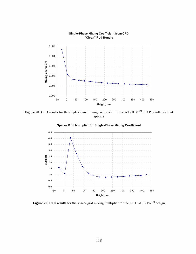
Single-Phase Mixing Coefficient from CFD"Clean" Rod Bundle

0.000

0.001

0.002

0.003

0.004

0.005M

ixi

g co

efci

ent

-50 0 50 100 150 200 250 300 350 400 450

Height, mm

Figure 28: CFD results for the single-phase mixing coefficient for the ATRIUM

nfi

out spacers

TM10 XP bundle with

Spacer Grid Multiplier for Single-Phase Mixing Coefficient

0.0

0.5

1.0

1.5

Height, mm

2.0

3.5

-50 0 50 100 150 200 250 300 350 400 450

Mu

Figure 29: CFD results for the spacer grid mixing multiplier for the ULTRAFLOWTM design

2.5

3.0

ltipl

ier

4.0

4.5

118

5.3.6.3 F-COBRA-TF Calculations of ATRIUMTM10 XP Bundle with ULTRAFLOWTM

Spacers

There are seven grids with mixing vanes instrumented along the heated length of the

ATRIUMTM10 XP bundle. The axial locations of the spacers are depicted in Figure 30. Using the

CFD results for the spacer grid mixing multiplier shown in Figure 29, a two-dimensional (2D) table

for the axial distribution of the spacer multiplier along the heated length of the ATRIUMTM 10 XP

bundle was prepared. The distribution is given in Figure 31.

The layout of the F-COBRA-TF model is given in Figure 32. It is a full bundle model, which

con

E.,

197

.

According to the F-COBRA-TF turbulent mixing model, the amount of the crossflow between

two adjacent subchannels is proportional to the density and void fraction gradients and the turbulent

mixing coefficient is a proportionality coefficient. By that reason, subchannels with equal cross-

sists of 117 subchannels and a large water channel. There are 91 fuel rods in total and 10 of

them are part-length rods. The model includes an unheated inlet part with one structural grid.

The turbulent mixing model, utilized in the performed calculations, defines the single-phase

mixing coefficient using the correlation by Rogers and Rosehart (Rogers, J. T. and Rosehart, A.

5) and the Beus’ model for two-phase mixing (Beus, S. G., 1970).

The pressure losses in the vertical flow are modeled with Equation 4.1 using experimentally

defined subchannel loss coefficients.

Two F-COBRA-TF calculations were carried out. In the first one the standard spacer grid model

was used. In the second calculation, at the spacer grid locations the single-phase mixing coefficient,

as defined with the correlation by Rogers and Rosehart, was enhanced with the spacer mixing

multiplier obtained by the CFD pre-calculations. The enhancement can be seen in Figure 33

119

sectional flow area, but different power loadings were selected for comparative analyses. The one

with the lower peaking factor is called “cold channel”, and the other is called “hot channel”.

The impact of the new model on the mass and energy redistribution inside the bundle is shown

in Figure 34 through Figure 41. A strong increase of the lateral flow transfer by turbulent mixing is

seen for both phases near and shortly downstream of the mixing vanes. However, Figure 42 shows

that for this particular bundle geometry the magnitude of the crossflow by turbulent diffusion is far

smaller than the diversion crossflow. Therefore, significant changes in the overall fluid thermal-

hydraulic performance due to the increased turbulence cannot be observed.

Regarding the graphs on Figure 34 and Figure 42, it has to be clarified that the axial position of

2.8 m, where there is a change of the crossflow direction, corresponds to the end of the part-length

rods. It seems that although the chosen subchannels rfaces of part-length rods, the

fluid

Additionally, the computational performance and efficiency of the modified code version was

investigated. Comparisons of the code temporal convergence are given in Figure 43. It is clearly

indicated that the new model does not result in a prolonged CPU time.

Performed stability analyses showed no distortions in the code convergence on mass and heat

balance due to the new modeling. The shape of the graphs in Figure 44 and Figure 45 is defined by

the simulated step-wise increase of the total power: the power of 100% is assumed to be reached at

1.8 second, after which the code needs about 1.2 seconds to obtain a steady state solution.

do not contain su

behavior in those subchannels is also affected by the flow area expansion at that elevation.

120

3708 mm

End of the Heated Length

Beginning of the Heated Length

275 mm

512 mm

512 mm

512 mm

512 mm

512 mm

512 mm

0.029 mm

Mixing vanes Spacer grid

Figure 3 of the

0: Axial positions of the ULTRAFLOWTM mixing spacers along the heated lengthATRIUMTM10 XP bundle

Spacer Grid Multiplier for ULTRAFLOW DesignATRIUM 10 XP Bundle

0

1

2

3

4

5

0.0 0.5 1.0 1.5 2.0 2.5 3.0 3.5 4.0

Heated lenght, m

Mul

tiplie

r

Figu XP

bundle re 31: Axial distribution of the spacer multiplier along the heated length of the ATRIUMTM10

121

91

1 2 3 4 5 6 7 8 9 10 11

12 13 14 15 16 17 18 19 20 21 22

23 24 25 26 27 28 29 30 31 32 33

34 35 36 37 38 39 40 41 42 43 44

45 46 47 48 49 50 51 52 53 54 55

56 57 58 59 60 61 62 63 64

65 66 67 68 69 70 71 72 73

74 75 76 77 78 79 80 81 82 83 84

85 86 87 88 89 90 91 92 93 94 95

96 97 98 99 100 101 102 103 104 105 106

107 108 109 110 111 112 113 114 115 116 117

1 2 3 4 5 6 7 8 9 10

11 12 13 14 15 16 17 18 19 20

21 22 23 24 25 26 27 28 29 30

31 32 33 34 35 36 37 38 39 40

41 42 43 44 45 46 47

48 49 50 51 52 53 54

55 56 57 58 59 60 61

62 63 64 65 66 67 68 69 70 71

72 73 74 75 76 77 78 79 80 81

82 83 84 85 86 87 88 89 90

Figure 32: Layout of the F-COBRA-TF model of the ATRIUMTM10 XP bundle

Spacer Grid Effect in the Mixing Coefficient

0.00

0.01

0.02

0.03

0.04

0.05

0 1 2 3 4 5

Heated lenght, m

Mix

ing

Coef

ficie

nt

standard modelspacer grid model

Figure 33: M dels

ixing coefficient determined by the standard and the new F-COBRA-TF mo

122

Lateral Flow by Turbulent Mixing of Liquid

-0.0020

-0.0016

-0.0012

-0.0008

-0.0004

0.0000

0.0004

0 1 2 3 4 5

Axial position, m

Flow

rate

, kg/

sstandard modelspacer grid model

Figure 34: Liquid crossflow by turbulent mixing, ULTRAFLOWTM spacer

Lateral Flow by Turbulent Mixing of Vapor

-0.00005

0.00000

0.00005

0.00010

0 1 2 3 4 5

Axial position, m

Flow

rat

e, k

g/s


TMFigure 35: Vapor crossflow by turbulent mixing, ULTRAFLOW spacer

123

Void Fractionhot channel

0.0

0.1

0.2

0.3

0.4

0.5

0 1 2 3 4 5

Axial position, m

Vol

ume

frac

tion,

-


Fi

gure 36: Void fraction in the hotter subchannel, ULTRAFLOWTM spacer

Void Fractioncold channel

0.0

0.1

0.2

0.3

0.4

0.5

0 1 2 3 4 5

Axial position, m

Volu

me

fract

ion,

-


Fi

gure 37: Void fraction in the colder subchannel, ULTRAFLOWTM spacer

124

Flow Qualityhot channel

0.00

0.01

0.02

0.03

0.04

0.05

0 1 2 3 4 5

Axial position, m

Qua

lity,

-


Figure 38: Flow quality in the hotter subchannel, ULTRAFLOWTM spacer

Flow Qualitycold channel

0.00

0.01

0.02

0.03

0.04

0.05

0 1 2 3 4 5

Axial position, m

Qua

lity,

-


Figure 39: Flow quality in the colder subchannel, ULTRAFLOWTM pacer s

125

Enthalpy- Mixturehot channel

1200

1250

1300

1350

0 1 2 3 4 5

Axial position, m

Ent

halp

y, k

J/kg


Figure 40: Enthalp TM spacer

y distribution in the hotter subchannel, ULTRAFLOW

Enthalpy- Mixturecold channel

1200

1250

1300

1350

0 1 2 3 4 5

Axial position, m

Ent

halp

y, k

J/kg


Figure 41: E TM spacer nthalpy distribution in the colder subchannel, ULTRAFLOW

126

Lateral Flow Components

-0.008

-0.004

0.000

0.004

0.008

0 1 2 3 4 5

Axial position, m

Flow

rate

, kg/

stotalturbulent mixingvoid driftdiversion

Figure 42: Components of the total crossflow

Code Convergencetime step

0.00

0.20

0.40

0.60

0.80

1.00

0 100 200 300 400 500Time step number

CPU

time

per t

ime

step

, s


Figure 43: Comparison of the code temporal convergence

127

Mass Balance

-100

-50

50

viat

io fr

omte

ady

ate,

%

0

100

0 1 2 3 4 5

Time, s

Den

s s

tstandard modelspacer grid model

Figure 44: Comparison of the code convergence on mass balance

Heat Balance

50e, %

-100

100

5

Time, s

Dn

st

y st

at

-50

0

0 1 2 3 4

evia

tio fr

omea

d


Figure 45: Comparison of the code convergence on heat balance

128


A comprehensive review of the recent trends in the turbulent mixing modeling in subchannel

codes indicates that the enhancement in the turbulent diffusion due to spacer grids in rod bundles is

negl

-T

The F-COBRA-TF turbulent mixing model was modified to use pre-calculated CFD results for

the enhanced turbulence due to spacer grids in rod bundles. A procedure that can be considered as

an o

ected in most of the codes. The development of new models requires either carrying out costly

experiments or performing computational fluid dynamics simulations. CFD capabilities allow us to

model the fluid behavior on a very refined spatial mesh and therefore to model local flow patterns

such as turbulence in the flow near spacer grids which are not “seen” by analyses on a subchannel

level.

Two methodologies were proposed for evaluation of the single-phase mixing coefficient by

means of CFD calculations: by evaluation of the turbulent viscosity and by heat balance across the

gap between two adjacent subchannels. The performed studies indicated that the second approach

gives more stable and physically reasonable results and therefore it was chosen for implementation

into F-COBRA F.

ff-line coupling between a CDF and a subchannel code was developed and verified for the

particular case of ATRIUMTM10 XP bundle with ULTRAFLOWTM spacer. For now, validation of

the model is not possible due to lack of suitable experimental data.

129

CHAPTER 6

MODELING OF DIRECTED CROSSFLOW CREATED BY SPACER GRIDS

6.1 Background

The crossflow in rod bundles can be divided into three categories: turbulent mixing, void drift,

and diversion crossflow. Additionally, some spacer designs create specific lateral flow patterns due

to velocity deflection on their structural elements as the mixing vane blades. This kind of diversion

crossflow is very often referred as directed crossflow. In other words, the directed crossflow is a

flow pattern caused by the sweeping effects of the vanes or other grid structures. The magnitude of

the directed crossflow depends of the spacer geometry. Examples for spacer designs creating

direc

declination angle, etc. The subchannel codes usually do not

have

), which

utilizes a simplified directed crossflow model. However, the work of Krulikowski (Krulikowski, T.

E., 1997) has shown that the model needs further improvements and more extensive validation.

ted crossflow are the HTPTM and FOCUSTM spacers (both are trademarks of AREVA NP

GmbH). Schematics of both designs are shown in Figure 46 and Figure 47. The HTPTM design has

a specific shape at the rod-to-rod gap regions that directs the flow to enter or leave the subchannel.

In the FOCUSTM design the mixing vanes configuration (mirrored and rotated in 90 degree) leads to

coexistence of an intra-subchannel swirling flow and a crossflow meandering in opposite directions

within one subchannel.

A correct modeling of the directed crossflow would require detailed geometrical information

such as vanes length and orientation,

advanced mechanistic models for evaluation of the lateral flow rates specified by a change of

the axial velocity vector. An exception is the COBRA-IV code (Stewart, S. W. et al., 1977

130

Figure 46: Schematic of the HTPTM Spacer Figure 47: Schematic of the FOCUSTM Spacer

A very coarse approach is still used in the subchannel analyses: the cont of l

convection to the crossflow is approximated by artificially increasing the single-phase mixing

im

bun

in the medium and should not

depend on convective mechanisms.

must separate the treatment of the diffusive and the convective effects of the spacer grids.

ribution the latera

coefficient to calculate a crossflow with a magnitude sufficient to reproduce exper ental results of

the available mixing tests. In this way, the single-phase mixing coefficient combines the effects of

the turbulent diffusion and the forced convection by mixing devices or other discrepancies from the

dle symmetry. Such a methodology violates the physics behind the turbulent diffusion

approximation: the mixing rate is proportional to the gradients

To overcome the above discussed modeling deficiency, the new generation subchannel codes

131

6.2

The current version of F-COBRA-TF (as well as the PSU versions of COBRA-TF) does not

model the directed crossflow. To improve the code capabilities of simulating convective lateral

flows due to spacer grids in rod bundles, a new model based on CFD calculations was developed.

New F-COBRA-TF Model for Directed Crossflow by Spacer Grids

6.2.1 F-COBRA-TF Transverse Momentum Equations

In the variety of COBRA-TF code versions, including F-COBRA-TF, the lateral mass flow

rates are defined by solving the transverse momentum equations for each field: continuous liquid,

entrained liquid, and vapor.

Recalling Chapter 3, the generalized phasic momentum equation has the following form:

( ) ( ) ( ) Tkkkkkkkkkkkkkkk MMMPgUUU

t+++⋅∇+∇−=⋅∇+

∂τααραραρα (6.1)

where k

d∂ Γ

α is the average k-phase void fraction; kρ is the average k-phase density; kU is the average

k-phase velocity vector; g is the acceleration of gravity vector; k

τ is the average k-phase viscous

kstress tensor; ΓM is the average supply of m ntum to phase k due to mass transfer to phase k;

is the average drag force on phase k by the other phases; and is the average supply of

momentum to phase k due to turbulent mixing and void drift.

The F-COBRA-TF momentum equations are solved on a staggered mesh where the momentum

cell is centered on the scalar mesh cell boundary. The mesh cell for the transverse velocities is

shown in Figure 48. The finite-difference transverse momentum equations are given in Equations

6.2 through 6.4. Quantities that are evaluated at the old time carry the superscript . Donor cell

quantities that have th

ome

dkM T

kM

n

e superscript n are evaluated at the old time. ~

132

In the transverse momentum equations, the pressure force term and the velocities in the wall

and interfacial drag terms are new time values, while all other terms and variables are computed

using old time values. The rate of momentum efflux by transverse convection is given as the sum of

the momentum entering or leaving the cell through all transverse connections. M tum

convected by transverse velocities (that are in the direction of the transverse velocities being solved

for) is the sum of the momentum entering or leaving through mesh cell faces connected to the face

of the mesh cell for which the momentum equation is being solved. NKII is the number of mesh

cells facing the upstream face of the mesh cell and NKJJ is the number facing the downstream face

of convected out through the sides of the mesh cell by velocities that are

orthogonal to the velocity to be solved for, but lying in the same horizontal plane, is given by the

sum of the momentum convected into or out of cells connected to the sides of the transverse

momentum mesh cell. The number of cells connected to the mesh cell under consideration, whose

velocities are orthogonal to its velocity, is given by NG. The momentum convected through the top

and bottom of the mesh cell by vertical velocities is the sum of the momentum convected into (or

out of) cells connected to the top and bottom of the mesh cell and depends on the number of cells

onnected to the top (NKA) and bottom (NKB) of the mesh cell.

omen

the mesh cell. Momentum

c

Scalar Mesh Cell (II) Scalar Mesh Cell (JJ)

∆z

∆x

S

Vj NKII NKJJ

NKB

NKA

NG

Figure 48: F-COBRA-TF transverse momentum mesh cell

133

Vapor Phase ( ) ( )[ ]

( ) ( )[ ] ( ) ( )[ ] ( ) ( )

( ) ( )[ ] ( ) ( )[ ]

( ) ( ) ( )[ ]

( ) ( )[ ] ( )[ ]J

vapmom

J

Jn

entEn

liqEn

vapCnJentvapJentvapentvapi

nJliqvapJliqvapliqvapi

nvapvapvapwall

j

JJIIJJJJIIvap

j

NKA

IAlatIAvap

nvapvapvap

j

NKB

IBlatIBvap

nvapvapvap

J

NG

LJ

LL

onvap

nJvapvapvap

J

NKJJ

LJLL

nvap

nJvapvapvap

J

NKII

LJLL

nvap

nJvapvapvap

JJJvapvapvapvapvapvap

zS

zVVW

WWWWK

WWWWKWWKz

xSPP

z

AUW

z

AUW

z

xSWW

z

xSWW

z

xSWW

t

xSWW

J

J

JJJJ

IAIB

∆+

∆

Γ−Γ−−Γ−−−−−

−−−−−−∆

∆−−

∆−

∆+

∆

∆⎥⎦⎤

⎢⎣⎡

+∆

∆−

∆

∆+

=∆

∆−

−

==

===

∑∑

∑∑∑

)_()_,(

)_,(_

1

~

1

~

1

~

1

~

1

~

12

22)()(

2

ηη

α

ραρα

ραραρα

ραρα

(6.2)

Continuous Liquid Phase

n

( ) ( )[ ]

( ) ( )[ ] ( ) ( )[ ] ( ) ( )

( ) ( )[ ] ( ) ( )[ ]

( ) ( ) ( )[ ] ( ) ( )[ ]

J

liqmomSJ)_(

Entrained Liquid Phase

J

Jn

liqEn

vapCnJliqvapJliqvapliqvapi

nliqliqliqwall

j

JJIIJJJJIIliq

j

NKA

IAlatIAliq

nliqliqliq

j

NKB

IBlatIBvap

nliqliqliq

J

NG

LJ

LL

onliq

nJliqliqliq

J

NKJJ

LJLL

nvap

nJliqliqliq

J

NKII

LJLL

nliq

nJliqliqliq

JJJ

nliqliqliqliqliqliq

z

zVW

WWWWKWWK

zxSPP

z

AUW

z

AUW

z

xSWW

z

xSWW

z

xSWW

t

xSWW

JJJJ

IAIB

∆+

∆

Γ−−Γ−−−−−+−−

∆

∆−−

∆−

∆+

∆

∆⎥⎦⎤

⎢⎣⎡

+∆

∆−

∆

∆+

=∆

∆−

−==

===

∑∑

∑∑∑

)_,(_

1

~

1

~

1

~

1

~

1

~

1122

)()(

2

ηη

αραρα

ραραρα

ραρα

(6.3)

( ) ( )[ ]

( ) ( )[ ] ( ) ( )[ ] ( ) ( )

( ) ( )[ ] ( ) ( )[ ]

( ) ( ) ( )[ ] [ ]

Jz∆entmom

J

Jn

entEn

vapCnJentvapJentvapentvapi

nentententwall

j

JJIIJJJJIIent

j

NKA

IAlatIA

nent

j

NKB

latIBentn

entliqent

J

NGLonn

J

NKJJ

L

nn

J

NKII

LJLL

nent

nJentliqent

JJentliqententliqent

Sz

VWWWWKWWK

zxSPP

z

AUW

z

AUW

xSWWxSWW

z

xSWW

xSWW

J

JJJJ

IAIB

+

∆

Γ−Γ−−−−+−

∆∆−

−∆

−∆

∆⎤⎡∆−

∆

∆+

∆−

−=

==

∑∑

∑∑∑

)_(

)_,(_

1

~

1

~

~~

1

~

22

)()(

ηη

αραρα

ραραρα

ραρα

(6.4) ententliq

IB+ =

LJLentJentliqentJLLentJentliqent

zz ∆

⎥⎦⎢⎣+∆

=11 2

J

n

t=

∆

W−

134

( )

The terms in the phasic transverse momentum equations can be described as follows:

( ) ( )

( ) ( )( )

( )( )

( ) ( ) ⎥⎦⎢⎣⎥⎦

⎢⎣

⎥⎦ zzvapentizzvapliqi A _,'''

_,τ( )

⎥⎦

⎤

⎢⎢⎢

⎣

⎡

+Γ+

⎥⎤

⎢⎡

⎤⎡

⎢⎣

⎥⎤

⎢⎡

∂−

−⎥⎤

⎢⎡

∂−

⎥⎤

⎢⎢⎢

⎣

⎡∂+

⎥⎥

⎦

⎤

⎢⎢

⎣

⎡+

⎥⎥⎥

⎦

⎤⎢⎡

∂∂

−−⎥

⎢⎢⎢

⎣∂

⎤⎡

∑

momkk

zzkwall

zkkkk

NG

oNGNG

okkkk

zkkkk

SWWbetwTransferMass

todueExchangeMomentumTransverse

ADropsandVaporbetweenDragIterfacial

A

PforceGradientessure

AUWVerticalbyEffluxMomentumTransverseofRate

AUWVerticalbyEffluxMomentumTransverseofRate

SWWConvectionTransverseOrthogonalbyEffluxMomentumTransverseofRate

zAWW

ConvectionSideJJ

TransversebyEffluxMomentumTransverseofRateAWW

A

MomentumTransverseofchangeofRate

Pr

''''''_ ττ

ρα

ραρα

ραρα

d at the beginning of the

current time step and are assumed to remain constant during the remainder of the time step. The

semi-implicit mom

+

⎥⎦

⎤⎢⎣

⎡+⎥

⎥STermSource

MomentumTransversefieldseen

±⎥⎥

⎢⎢

±⎥⎤

⎢⎡

−

⎥⎦

⎢⎣ ∂⎥

⎥⎦⎢

⎢⎣ ∂ zk

IA

LiquidContinuousandVaporbetweenDragIterfacialShearWallTransverse

LA

zaboveConvection )( α

⎥⎥⎦∂

IBzkkkk

zbelowConvection )(

⎢⎢⎣⎥

⎥⎦∂

− zkkkk

zConvectionSideII

⎤⎡

=⎥⎥⎥

⎦⎢⎢⎢

⎣ ∂∂ kkk

TransversebyEffluxMomentumTransverseofRatet

Wρα

The equations are solved first using currently known values for all variables to obtain an

estimate of the new time flow. All explicit terms and variables are compute

entum equations have the form:

entvapliq memdmcPbm &&&& +++∆= (6.5)

where vapliqliq mdmcPbam &&& 1111 ++∆+= ; entvapliqvap memdmcPbam &&&& 22222 +

a

++∆+= ;

and dPbam& 33 +∆+= entvapent mem && 33 + .

The constants a1, a2, and a3 (in represent the explicit terms such as momentum efflux skg / )

135

terms and the gravitational force; b1, b2, and b3 (in sm ⋅ ) are the explicit portion of the pressure

gradient force term; c1 and c2 (in ) are explicit factors that multiply the liquid flow rate in the

wall and interfacial drag terms; 2, d3, e2, and e3 (in ) are the corresponding terms that

multiply the vapor and entrained liquid flow rates.

The equations can be written in a matrix form as

(6.6)

and then solved by Gaussian elimination to obtain a solution for the phasic mass flow rates as a

function of the pressure gradient across the momentum cell,

2m

d1, d 2m

⎪⎭

⎪⎬

⎫

⎪⎩

⎪⎨

⎧

∆−−∆−−∆−−

=⎪⎭

⎪⎬

⎫

⎪⎩

⎪⎨

⎧

⎥⎥⎥

⎦

⎤

⎢⎢⎢

⎣

⎡

−−

−

PbaPbaPba

m

m

m

ededc

dc

ent

vap

liq

33

22

11

33

222

11

101

01

&

&

&

P∆ :

(6.7a)

p ∆−= 22& (6.7b)

∆−= 3& c)

Phgmliq ∆−= 11&

Phgmva

m Phgent 3 (6.7

In regard to the new spacer grid model, the rate of change of momentum by directed crossflow

can be added to the coefficients a in Equation 6.5, which are calculated as

⎟⎠

⎜⎝ ∆∆

=ty

a , ⎞⎛ ∆∆ It (6.8)

where is the time difference (time step size),t∆ y∆ is the spatial difference (gap length), and tI

∆∆

is the change of momentum. Thus, the total rate of momentum change in transverse directions will

be modified as follows:

136

( ) [ ]

( ) ( )

( ) ( )( )

( )( )

( ) ( )

⎤

⎢⎢

⎡

±⎥⎥⎦⎢

⎢⎣

−

⎥⎥

⎦

⎤

⎢⎢

⎣

⎡

∂∂

−−

⎥⎥⎥

⎦

⎤

⎢⎢⎢

⎣

⎡

∂∂−

⎥⎥⎦⎢

⎢⎣ ∂

+⎥⎥

⎦⎢⎢

⎣+

⎥

⎥

⎦

⎤

⎢

( )

⎦⎣⎥⎥⎦⎢

⎢⎢

⎣

⎡

+Γ+

⎥⎥⎦

⎤

⎢⎢⎣

⎡±

⎥⎥⎥

⎦

⎢

⎣

⎤⎡

⎥⎤

⎢⎡

∂⎤⎡

⎥⎢

⎥⎤

⎢⎡

+⎥⎤

MomentumTransversefieldsbetween

todueExchangeomentum

⎢

⎣−⎥⎢

⎢⎡

∂−

+

±=⎥⎥⎦

∂

momkk

zzvapentizzvapliqi

zk

kk

zkkkkzkkkk

STermSourceSWW

TransferMassMTransverse

ADropsandVaporbetweenDragIterfacial

A

ShearWallTransverse

A

essure

aboveConvection

WVerticalbyEffluxMomentumTransverseofRateOrthogonalbyEffluxMomentumTransverseofRate

ConvectionSideJJConvectionSideII

W

)(

)

ossflowDirectedCrbyEffluxMomentumTransverseofRate

'''_,

_,

τ

α

ρα

ρα

6.2.2 Ca

f the new methodology for CFD based subchannel modeling of the

directed crossflow the goal was to establish a model that: 1) represents the convective nature of the

phenomenon; 2) is simple and can be easily implemented into the subchannel momentum

equations; and 3) is effic

ach d re for

preliminary investigations. While the first two candidates utilize CFD predictions for the velocity

curl in a lateral plane for evaluation of the lateral momentum change, the third candidate uses CFD

pred

⎡

∂∂−

⎥

⎥

⎦

⎤

⎢⎣∂

∑

zzkwall

IAzkkkk

IBzkk

NG

oNGNG

okkkk

LiquidContinuousandVaporbetweenDragIterfacial

A

LP

forceGradient

zAUW

VerticalbyEffluxMomentumTransverseofRatez

AUbelowConvectionSWWConvectionTransverse

zAWW

TransversebyEffluxMomentumTransverseofRate

zAWW

TransversebyEffluxMomentumTransverseofRate

Pr

(

''''''

_ ττ

ρα

ρα

ραρα

⎥⎤

⎢⎢⎢

⎣

⎡

∂kkk

tA

MomentumTransverseofchangeofRate

lculation of the Transverse Momentum Change by Directed Crossflow

During the development o

ient in regard to the CPU time.

Three alternative modeling appro es (the so-called can idates) were conside d

iction for the lateral velocity. Based on performed comparative analyses the third candidate was

selected for further development since it performs with a high accuracy and is numerically stable.

137

Short descriptions of candidates 1 and 2 are given in Appendix D. The description of the third

method is following hereinafter.

Consider two fluid volumes, geometrically fully identical, connected to each other through a

gap with an area xSA ∆= (see Figure 49). The fluid in both volumes is at isothermal conditionsijlat

and is moving in axial direction x with a constant velocity inletUU ≡ . Assume that at given

elevation along the length there exits a force that results in a non-zero fluid velocity in the

lateral direction . Since, the model is constructed to avoid pressure and temperature gradients in a

lateral plane, the force can be defined as

, (6.9)

where

is the mass flow rate in direction equal to

F V

y

VmF lat&=

latm& y

latlat AVm ρ=& , (6.10)

where ρ is the fluid density.

Then, the force acting on the fluid in the gap region will be given as

(6.11)

and it is equal to the momentum change

latlat AVVmF ρ2== &

latI∆ in the lateral direction over a time interval y t∆ :

latlat

lat AVFt

II& ρ2=≡∆∆

= . (6.12)

Consider now a rod bundle of geometrically identical subchannels with uniform distribution of

the power and the inlet flow. Let obstacles exist in each subchannel and cause a change of the

138

velocity vectors, which results in a non-zero lateral flow. At such conditions the crossflows existing

in th

nfigurations in

fuel rod bundles - the coefficients a in Equation 6.8 can be corrected to account for the additional

momentum change as calculated by Equation 6.12. However, the lateral velocity predicted with

the

e bundle will be only due to velocity deflection on the obstacles. If we can predict in advance

the magnitude and the direction of the resulting lateral velocities, the above described model can be

used for prediction of the lateral momentum change due to specific mixing vane co

latI&

CFD code will account for the transverse pressure losses due to skin friction on the rods.

Therefore, action has to be taken either to correct the CFD results or to terminate the modeling of the

transverse friction pressure losses in the subchannel model.

ijSChannel i Channel j

x∆

y

x

flow

Figure 49: Schematic of two intra-connected fluid volumes

The subchannel analysis codes are not able to calculate such local changes in the velocity field.

Fortunately, we ca

n utilize the features of computational fluid dynamics to evaluate the lateral

139

velo

ted bundle correspond to ones used in the CFD calculations, the

forc

(6.13)

pre-calculations for each particular case to be simulated with the

subcha od axial velocity, which is

assu

w

u

c

l

c

m

city across the gaps between the adjacent subchannels.

Under the consideration that the inlet fluid velocity, the fluid density, and the area available for

lateral flow exchange in the simula

e to be added to the momentum equations of the subchannel code can be given as

CFDlat

CFDCFDCFDCFDlatSGlat AVVmF ρ2

_ )(== &

However, since the CFD calculations are costly in regard to the computational time, it is

inefficient to perform CFD

nnel c e. Moreover, the CFD calculations are performed at given

med to remain constant over the axial length. This is not the case of the subchannel analysis,

here not only the inlet velocity could be different form the one used in the CFD predictions, but it

sually varies along the axial length. Therefore, the model has to be made applicable to any flow

onditions to be simulated by the subchannel code, or in other worlds, the CFD predictions for the

ateral velocity have to be scaled to the actual subchannel conditions. The scaled lateral velocity *V

an be further used for calculation of the force SGlatF _ to be added to the subchannel code

omentum equation:

*_ Vm

tI

latSGlat ∆∆

The scaling involves the definition of the ratio of the lateral velocity as predicted by the CFD

ode and the inlet axial ve

F SCH&== (6.14)

c locity in the CFD model, the so-called spacer grid lateral convection

factor:

CFDinlet

CFD

UV

SGlatf =_ . (6.15)

140

It is dimensionless parameter that gives the information how the magnitude of lateral velocity

epends on the magnitude of the inlet velocity. The spacer grid lateral convection factor is a function

f the axial distance from the grid.

During the evaluation of the subchannel crossflow SCHm& , the F-COBRA-TF donor cell logic

d

o

and upwind discretization approach have to be taken into account.

Implying such a scaling procedure will reduce the required CFD pre-calculations to modeling of

the sample geometries only.

6.2.3 Verification of the Proposed Directed Crossflow Model

The functionality of the new model was verified against CFD simulations. A 2×2 channels

model of FOCUSTM spacers was developed at AREVA NP GmbH. It consists of four geometrically

identical subchannels arranged in a 2×2 array. The fluid in all four subchannels is water at

temperature of 300 °C and inlet axial velocity of 5 m/s. There are no heated walls. The fluid

properties remain constant along the axial length. The spacer grid configuration is such that each

subchannel contai ate intra-channel

wirl downstream of their top edges and directed crossflow between adjacent subchannels with

meandering patterns. The mixing vanes configuration is shown in Figure 50. 3D views of the

FOCUSTM spacer is given in Figure 51. The chosen fluid conditions assure no diffusive effects due

temperature gradient and therefore lateral flows are driven only by convective processes. The model

is summarized in Table 7.

In total four CFD calculations were performed, in which the mixing vane angle varied from 10

to 40 degree. The lateral (UW) velocities were extracted at every 10 mm axial distance. The CFD

results for flow distribution -3 of Appendix E. It was

lat

ns a pair of two rotated and mirrored mixing vanes, which cre

s

are given in Table E-1 through Table E

141

observed that immediately downstream of the grid the lateral flow structures exhibit swirling flow

created by the m

neighboring subchannels are rotating in opposite directions and thus creating a crossflow through

the gaps. The magnitude of the swirl, and respectively the magnitude of the crossflow, is decreasing

further downstream of the spacer. Larger is the mixing vane angle, stronger is the crossflow.

ixing vanes. Because the mixing vanes were mirrored, the swirls in any two

Figure 50: Mixing vanes configuration in the 2×2 FOCUSTM model

Figure 51: 3D views of the FOCUSTM spacer

142

Table 7: Description of the 2x2 channels model used in the STAR-CD calculations

rod diameter 9.5 mmpitch 12.7 mm

Inlet velocity

Thermal Hydraulic Analyses of Flow and Heat TransferCoupled Subchannel Analyses

to study flow distribution with cross flownet mass transfer between the subchannels by directed crossflow

Characterization of Runcoupled 2 x 2 subchannelschannels with equal inlet velocities and temperaturesmirrord and rotated mixing vanes

Objective

length 540 mm5 m/s

strip thickness of 0.4 mm, vane angle 10°, 20°, 30°, and 40°

Specific heat 4457,3333 J/kg/K

Discretization Upwind

STAR-CD Calculation

Model

Outlet Outlet / Pressure conditionGaps between rods symmetry conditionWalls no-slip, adiabatic, smoothTemperature at inlet 300°CTurbulence at inlet Intensity 5%, length 2 mmDensity 727.46 kg/m³Lam. Viscosity 8.8688e-5 kg/m/sThermal conductivity 0.56 W/m²/K

Solver Simple, CG + AMG

Accuracy 0.0001Turbulence standard k-ε, wall fucnctiontypical cell dimension 0.3 mm

Method

Properties

Boundary Conditions

From the axial distribution of the lateral velocities, shown in Figure E-1 through Figure E-4 of

Appendix E, it is seen that for small declination angles (10 degrees) lateral velocities through all the

gaps are equal in magnitude and have same distribution over the axial length. However, for the

larger angles the distribution is not longer symmetrical. Lateral velocities through the east and south

gaps have similar qualitative and quantitative behavior. One very interesting finding is the change

of the velocity direction (sign) at 30/36 hydraulic diameters downstream of the mixing vanes.

Lateral velocities through the west and north gaps also have similar magnitude and axial

distribution, but there is no change of the sign. Table E-2 and Table E-3 of Appendix E show the

143

lateral velocity field further downstream of the spacer. The asymmetry effect might be caused by a

migration of the swirling flow away from the center of the subchannel when the flow is developing

downstream of the vanes. For example (Table E-2), in the north-east and south-east subchannels the

centers of swirling flow move away from the east gap leading to less crossflow through it. At the

same time, in the north-west and the north-east gap the swirls move toward the north gap and thus

creating crossflow through that gap. Nevertheless that such an effect might be characterized as a

numerical problem of the CFD calculations, very similar experimental results were reported by

Conner (Conner, M. E. et al., 2004).

As above mentioned, the axial distributions of the lateral velocity over one spacer grid span

were not symmetrical for large declination angles. However, for the following studies the lateral

velocities w

The CFD predictions for the lateral velocity and the lateral mass flux are shown in Figure 52 and

Figure 53. The lateral convection factors , evaluated with Equation 6.15, are plotted in

Figure 54. In these figures the length is extended to 3 m, which corresponds to the heated length of

the 5×5 rod bundle with FOCUSTM spacer, which will be used later for validation of the model.

There are five spacer grids instrumented along the length as depicted in Figure 55.

ere averaged over the four gaps and a single value was used in the performed analyses.

SGlatf _

144

Lateral VelocityCFD

0,00

0,25

0,50

0,75

1,00

1,25

1,50

1,75

2,00

0,0 0,5 1,0 1,5 2,0 2,5 3,0 3,5

Axial elevat on, mi

Velo

city

, m/s 10 deg

20 deg30 deg40 deg

Figure 52: CFD predictions for the lateral velocity for different mixing vane angles

Lateral Mass FluxCFD

0

250

500

750

1000

1250

1500

0.0 0.5 1.0 1.5 2.0 2.5 3.0

Axial elevation, m

Mas

s flu

x, k

g/m

2 s

10 deg20 deg30 deg40 deg

Figure 53: CFD predictions for the lateral mass flux for different m xing vane angles i

145

146

Lateral Convection Factor

0.2

0.4

lat_

conv

0.0

0.1

0.3

0.0 0.5 1.0 1.5 2.0 2.5 3.0

Axial position, m

F, -


Figure 54: Lateral convection factor for different mixing vane angles

Figure 55: Schematic of the spacers positions in the 5x5 bundle with FOCUSTM spacer

3 m

EOHL

BOHL0.275 m

0.545 m

0.545 m

0.545 m

0.04 m

0.545 m

The data exchange between the CFD code and the subchannel code is similar to one described

in Section 5.3.4. An interface module was developed, which 1) contains detailed information for the

lateral convection factor in a 2D table format; 2) contains additional information for the orientation

of the directed crossflows in regard to the global coordinate system; and 3) maintains the exchange

between the CFD data base and F-COBRA-TF. Again, for the purposes of routine safety analyses,

the code can be supplied with sets of data representing spacer designs that are currently used. For

new design studies, an “experienced” user can create a new data set based on more recent CFD

calculations.

The flow chart of the directed crossflow modeling and examples for the obtained CFD data sets

of the lateral convection factor are given in Appendix F.

F-C t. The

predicted lateral velocity and mass flux are shown in Figure 56 and Figure 57. It can be seen that

the proposed methodology is able to reproduce the axial variation of the lateral mass flux between

the adjacent subchannels in both qualitative and quantitative manners.

The obtained results demonstrate the functionality of the proposed methodology and therefore

the model was implemented in the latest version F-COBRA-TF for simulation of directed crossflow

created by different velocity deflectors. The validation of the new modeling is presented in the next

section.

OBRA-TF simulations of the 2×2 channel model of FOCUSTM spacer were carried ou

147

Lateral VelocityF-COBRA-TF

0,00

0,25

0,0

0,50

1,00

2,00

0,5 1,0 1,5 2,0 2,5 3,0 3,5

Axial elevation, m

loci

t

1,25

1,50

1,75

y,m

/s 10 deg20 deg30 deg40 deg0,75Ve

Figure 56: F-COBRA-TF predictions for the lateral velocity for different mixing vane angles

Lateral Mass FluxF OBRA-TF

1000

1250

1500

/m2 s

-C

s f

g

0

250

500

750

0.0 0.5 1.0 1.5 2.0 2.5 3.0 3.5

Axial elevation, m

Mas

lux,

k


the lateral mass flux for different mixing vane angles

Figure 57: F-COBRA-TF predictions for

148

6.2.4 Validation of the Proposed Directed Crossflow Model

experiments performed with SIEMENS Test Section 53 (DTS53) were used for

validation of the proposed model. The tests were conducted at the Columbia University, New York

in 1990 for SIEMENS KWU (AREVA NP GmbH) PWR test section TDS53. The bundle

d easured data for are available in Vogel, Chr. et al., 1991.

ption of the DTS53 Ex

Mixing

escription and m

6.2.4.1 Descri periment

In total twenty-one tests were performed in a 5×5 rod bundle array. The bundle geometry is

s le 8.

ution was no xteen peripheral rods had a relative power

0.94 and the nine internal rods had a relative power of 1.11. The axial power distribution was

ve d

e bund equipped CUSTM s rids with inlet edges dimples,

a agonal nted spring trips have ss of 0.45 nd height o m. Split

m vane attached a per edge o rip. Ther e spacers a e heated

l equidi distributed span of 54 see Figur

e exp tal data i exit subc fluid tem es in a 6× trix and

differential pressure drop me nts. The nties of erature measurements are

r d bein een 0.61 a for the a temperatu e range of 2 o 343 ºC

( tti, C. 1990). If t asured tem re by 5

d s, it w t to a nega alue in th base. The total error in ab pressure

m rements is reported being ± 0.41 bars.

ummarized in Tab

The radial power distrib nuniform: the si

of

uniform l c. The operationa onditions are gi n in Table 9 an Table 10.

Th le was with FO pacer g straight , oval

nd di ly orie s. The s thickne 3 mm a f 40 m

ixing s were t the up f the st e are fiv long th

ength stantly with a 5 mm ( e 55).

Th erimen nclude hannel peratur 6 ma

asureme uncertai the temp

eporte g betw nd 1.0 K bsolute re in th 05 ºC t

Fighe et al., he me perature exceeded the saturation temperatu

egree as se tive v e data solute

easu

149

Table t section DTS53

Pa

8: Geometrical characteristics of tes

rameter Value Lattice 5×5 Number of heater rods 25 Number of guide tubes 0 Pitch, m 0.0127 Heater rod outside diameter, m 0.0095 Heated length, m 3 Rod to wall clearance, m 0.00314 Corner radius, m 0.0004 Bundle flow area, m2 0.0026607

Table 9: Range of conditions for test section DTS53

Parameter Range Exit pressure, bar 159.2 ÷ 160.6 Fluid inlet temperature, ºC 203.6 ÷ 282.1 Average mass flux, kg/m2-s 3546.4 ÷ 3655.7 Bundle power, kW 1162.9 ÷ 4620.9

Table 10: Tests operational conditions

Test Inlet Flow Rate, kg/s

Inlet Enthalpy, kJ/kg

Bundle Power, kW

Exit Pressure, bars

Inlet Temperature, ºC

08.0 9.619 1238.7 3005.6 159.60 281.2 09.0 9.518 1239.6 3053.0 159.90 281.4 10.0 9.501 1241.6 3043.6 159.60 281.8 11.0 9.654 1238.4 2123.8 159.60 281.2 12.0 9.663 1236.2 2126.8 159.60 280.7 13.0 9.689 1234.3 2137.7 159.20 280.3 14.0 9.564 1240.4 1162.9 159.60 281.5 15.0 9.587 1239.7 1168.6 160.60 281.4 16.0 9.727 1089.9 2695.3 160.30 250.8 17.0 9.693 1078.8 2624.5 159.90 248.4 18.0 9.618 1084.2 2621.3 160.60 249.6 19.0 9.436 1079.9 2807.0 159.60 248.7 20.0 9.574 1080.6 3798.6 159.90 248.8 21.0 9.563 1090.1 3784.2 160.60 250.8 22.0 9.559 887.4 2976.0 159.60 206.5 23.0 9.566 887.5 2957.7 159.60 206.5 24.0 9.580 877.5 2944.3 159.90 204.3 25.0 9.502 889.2 3711.6 160.60 206.9 26.0 9.551 886.5 4620.9 159.90 206.3 27.0 9.659 1077.4 4470.9 159.90 248.1 28.0 9.585 1094.3 4435.1 160.30 251.7

150

6.2.4.2 F-COBRA-TF Model

F-COBRA-TF model of the 5×5 bundle was developed. It is a full bundle model that consists of

36 subchannels, each divided into 75 equidistant axial nodes of 40 mm height. Geometrical

characteristics are given in Table 11.

A schematic of the model is shown in Figure 58 and the mixing vanes arrangement and

me

Inlet boundary conditions of flow rate and enthalpy and exit boundary conditions of pressure

are applied.

The spacer gr odeled as velocity head rtical flow. An average value

of 1.12 for the p cification, is applied to all

subchannels.

Experimental conditions and the bundle geometry ar result in a lateral mass flux

caused by 1) turbulent mixing due to density and void fraction gradients; 2) diversion crossflow due

to lateral pressur low due to velocity deflection on the mixing

vanes surfaces.

Turbulent mixing is modeled using a single-phase icient, as predicted with the

correlation by Ro T. and R. G., 1972) and Beus’ model

(Beus, S. G., 1970 mix

The directed crossflow model requires additional input information for the orientation (sign) of

the directed crossflow. The F-COBRA-TF logic for lateral flows assumes a positive flow from a

low-numbered subchannel to a high-numbered subchannel. If the crossflow has an opposite

direction it is considered negative. Therefore the orientation of the directed crossflow created by the

andering flow patterns established in the bundle are illustrated in Figure 59.

ids effects are m losses in a ve

ressure loss coefficient, as provided in the tests spe

e expected to

e gradients; and 3) directed crossf

mixing coeff

gers and Rosehart (Rogers, J. Rosehart,

) for enhanced two-phase turbulent ing.

151

mixing vanes has to be specified in advance. This information is supplied by an additional input file

(dirct_data.inp in Figure F-1 of Appendix F). A negative sign following the gap numbers in Figure

58 indicates that the crossflow is directed from a high-numbered subchannel to a low-numbered

subchannel, and vise versa, a positive sign indicate at the crossfl is directed from a low-

numbered subchannel to a high-numbered subchannel.

Another required input is the declination angle of the mixing vanes. For the FOCUSTM spacer it

is 22 degrees.

Table 11: Geometrical characteristics of the F-COBRA-TF model

Corner Subchan

s th ow

nel Flow area, m2 0 4496 .00004Wetted perimeter, m 0.021985442 Gap width to side subchannel, m 0.00314 Gap length to side subchannel, m 0.010295 Side Subchannel Flow area, m2 0.000064762 Wetted perimeter, m 0.027622565 Gap width to corner subchannel, m 0.00314 Gap length to corner subchannel, m 0.010295 Gap width to side subchannel, m 0.00314 Gap length to side subchannel, m 0.012700 Gap width to internal subchannel, m 0.00320 Gap length to internal subchannel, m 0.010295 Internal Subchannel Flow area, m2 0.000090408 Wetted perimeter, m 0.029845130 Gap width to side subchannel, m 0.00320 Gap length to side subchannel, m 0.010295 Gap width to internal subchannel, m 0.00320 Gap length to internal subchannel, m 0.012700

152

2 - 4 + 6 - 8 + 10

1 + 3 - 5 + 7 - 9 + 11

1 2

12 -42 -

41 + 43 - 13 +

14 +

16 -

17 +

18 +

20 -22 +

48 -

24 -

50 +

26 +

52 -

28

30 -

31 + 53 -

34 -

35 +

36 +

37 +

38 -

39 -

40 +

44 -56 +

- 46 +

51 + 49 - 47 -

15 -33 -

32 +

45 + 55 +

54 - 60

19 -21 - 23 + 25 -27 + 29

3 4 5 6

7

8

9

10

1112131415 16

17

18

19

20 21 22 23 24

25

26

27282930

31

32 33 34

3536

1 2 3 4 5

16 17 18 19 6

14 22 8

15 24 25 20 7

23 21

13 12 11 10 9

58 -

Figure 58: Schematic of the F-COBRA-TF 5×5 model of DTS53 mixing test bundle

59 - 57 +

Figure 59: Mixing vanes arrangement and meandering flow patterns in the 5x5 bundle with FOCUS spacer

TM

153

6.2.4.3 F-COBRA-TF Results

calculations of the TDS53 experiments were carried out utilizing four different

mo

F-COBRA-TF

deling options:

OPTION 1:

The spacer grid effects are modeled by pressure losses in a vertical flow. A pressure loss

coefficient of 1.12 is applied to all subchannels.

The turbulent mixing is modeled with the correlation by Rogers and Rosehart for the single-

phase mixing coefficient (Rogers, J. T. and Rosehart, R. G., 1972) and Beus’ model for two-phase

mixing (Beus, S. G., 1970).

OPTION 2:

The spacer grid effects are modeled by pressure losses in a vertical flow and a directed

cro


pha

OPTION 3:

ssflow modeled for all the gaps. A pressure loss coefficient of 1.12 is applied to all subchannels.

se mixing coefficient (Rogers, J. T. and Rosehart, R. G., 1972) and Beus’ model for two-phase

mixing (Beus, S. G., 1970)

The spacer grid effects are modeled by pressure losses in a vertical flow and a directed

crossflow modeled for the internal gaps only (gaps between internal subchannels). A pressure loss

phase mixing coefficient (Rogers, J. T. and Rosehart, R. G., 1972) and Beus’ model for two-phase



154

mix

OPTION 4:

ing (Beus, S. G., 1970).

The spacer grid re modeled by pre oss


The turbulent mixing is modeled by a single-phase mixing coefficient of 0.04, which is a value

found by fitting the COBRA 3CP res

The reason for introducing Option 3 is that the CFD data for the lateral velocity were evaluated

only for the particular configuration of 2×2 array of identical subchannels. In our case, 5×5 bundle,

those correspond to the four central subchannels. There is no CFD data currently available for the

other geometrical c tions found in the s els,

side-to-side subchannels, and corner-to-side subchannels).

The reason for introducing Option 4 is to compare the results obtained with the new model to

the ones obtained with the current a

An automatic procedure, the so-called 5×5 mixing test matrix, for input decks generation, code

ation was created for the DTS53 mixing

exp

The F-COBRA-TF predictions for the mixture temperature at the subchannels exits were

compar ch test point (the so-called run) the mean values and the

standard deviations of the absolute temperature difference

effects a ssure losses in a vertical flow. A pressure l

ults to the experimental data.

onfigura imulated 5×5 bundle (internal-to-side subchann

pproach used in AREVA NP GmbH.

execution, and extraction of the necessary output inform

eriments.

ed to the measured data. For ea

expTTcalc − and the temperature

differen along the heated lengthce relative to the temperature rise inoutcalc

TTTT

expexp

exp

−

− were calculated as

follows:

155

Mean value of the absolute temperature differences absnT∆ :

N

TT

N

n

absn

abs∑=

∆=∆ 1 , where

ncalcabs

n TTT exp−=∆ (6.18)

Standard deviation of the absolute temperature differences absnT∆ :

( )∑=− nN 1

∆−∆=N

n

absabsabs TT1

21σ (6.19)

Mean value of the relative temperature differences relnT∆ :

NT nrel

Tn∑N

=

∆

n

=∆ 1 , where inoutcalcrel

n TTT exp

−=∆ (6.20)

Standard deviation of the relative temperature differences

TT

expexp

−

relnT∆ :

( )∑ ∆−∆=

= relrel TTσ (6.21)

Statistical analyses were performed for four data sets:

1) All subchannels;

ll internal subchannels;

−

N

nnN 1

2

11

where n is the number of analyzed test points (runs).

2) Peripheral subchannels only;

3) A

4) Four central subchannels only.

Results are given in Table 12 through Table 19. Table 20 shows the temperature differences

156

( )isubchannelcalc TT

_exp− for each subchannel i averaged over the calculated test points. There is no

value given for the first subchannel, because only two measured points are available for this

subchannel. Results can be summarized as follows:

1. The original F-COBRA-TF models, which do not simulate the change in the lateral

momentum due to velocity deflection, mispredict the fluid temperature distribution at the bundle

exit with 3.5 ºC in average. There is a strong overprediction for the central region of the bundle and

und

2. Applying an additional force calculated by Equation 6.14 to the all lateral momentum cells,

regardless of their location in the computational domain (Option 2), results in an improvement of

the

At the same time, there is an impressive improvement for the central subchannels: the mean

erprediction for the peripheral region. This is an indication that the lateral transfer is

underestimated by the code: the fluid surrounding the more heated rods in the central region is not

redistributed to the less heated peripheral subchannels.

overall prediction, but not for the peripheral region, where the calculated fluid temperature

becomes significantly overpredicted. In other words, the hotter fluid from the central part is

overforced to the bundle periphery. These results are not unexpected. We have applied a force,

which was calculated using lateral convection factor derived from CFD pre-calculations for

geometry corresponding to four central subchannels, to a very different configuration of adjacent

subchannels.

value of the absolute temperature differences is reduced from 6.8ºC in average to only 1.7ºC in

average.

3. Learning the lesson from the above discussed results, in the third set of evaluations (Option

3) the force was applied only to the gaps connecting internal-to-internal subchannels. Since, there

157

are no CFD pre-calculations for the corner-to-side, side-to-side, and side-to-internal subchannels

configurations, no force was applied to those gaps. Of course, this is not a truly physical approach,

incorrectly calculated rates of transverse momentum change will be not

applied to the subchannel equations. As it was expected, the re o significan

th red al nels he O

agreement with the expe ata pe bch is .

4 In the f set of luations ption 4 mode approa sed by EVA

GmbH for simu n of the DTS53 experiments was utilized: the crossf effects were mode

by a nhanced xing co ient of 4 for b single- two-ph flow c tions; t

value was found by fitting the COBRA 3CP results to the exp ental da t can b n that t

approach gives rse agr experim al data paring to Option 3.

T validati f the p sed mo g of di d cros in rod dles ag t AREV

NP GmbH DTS53 mixing experiments shows very promisin sults. N rtheles t the n

model was partially applied, due to the lack o l set o D dat alread ves be

repr tation o e flow ibution de rod dles th e rece used m dology

simu ng convective later ansfers with an en ed turb t mixing. This ind s that

ts, tu ent ixing and convective mixing, have to be modeled separately in the

momentum equations of the subchannel codes.

Additionally, the computational performance and efficiency of the modified code version was

investigated. Comparisons of the code temporal convergence are given in Figure 60. It can be seen

that the new model does not result in a prolonged CPU time.

Performed stability analyses showed no distortions in the code convergence on mass and heat

but it will assure that

sults show n t change in

e code p ictions for the intern and central subchan , as compared to t ption 2, but the

rimental d for the ripheral su annels improved

. orth eva (O ) the ling ch u AR NP

latio low led

n e mi effic 0.0 oth and ase ondi his

erim ta. I e see his

a wo eement with the ent com

he on o ropo delin recte sflow bun ains A

g re eve s tha ew

f ful f CF a, it y gi tter

esen f th distr insi bun an th ntly etho of

lati al tr hanc ulen icate the

two effec rbul m

158

balance due to the new modeling (Figure 61 and Figure 62).

Table 12: Statistical analyses for da and standard deviation of absolute temperature differences

Number Original F-COBRA- D h All Crossflow through

era TF Models,

ta set 1: all subchannels. Mean value

Run OPTION 1

TF Models

OPTION 2 irected Crossflow

throug Gaps

OPTION 3 No Directed

Periph l Gaps

OPTION 4 Original F-COBRA-

β = 0.04

Mean Value Deviation Value Deviation Value Deviation Value Deviation

Standard Mean Standard Mean Standard Mean Standard

8 3.5 2.7 2.9 2.1 2.5 2.1 2.6 1.8 9 3.3 2.4 2.9 2.1 2.5 1.9 2.6 1.9

10 3.6 2.5 3.1 2.4 2.7 2.3 3.0 2.1 11 2.3 1.6 2.2 1.6 1.8 1.5 2.0 1.5 12 2.3 1.7 2.2 1.6 1.8 1.5 2.0 1.5 13 2.3 1.6 2.1 1.5 1.7 1.4 1.9 1.4 14 1.6 1.1 1.6 1.4 1.4 1.1 1.5 1.3 15 1.5 1.1 1.4 1.2 1.2 1.0 1.3 1.2 16 3.1 2.2 3.2 1.9 2.7 1.7 2.9 1.8 17 3.3 2.0 2.9 1.9 2.5 1.8 2.7 1.8 18 3.4 2.0 2.9 2.0 2.5 1.9 2.7 1.7 19 4.1 2.6 3.2 2.3 2.9 2.1 3.0 2.0 20 4.0 2.9 3.5 1.9 2.9 1.8 3.2 1.5 21 4.1 2.9 3.5 1.9 2.9 1.7 3.3 1.6 22 4.4 3.0 3.5 2.3 2.9 2.3 3.2 2.1 23 4.2 2.9 3.8 2.5 3.2 2.4 3.5 2.1 24 4.1 2.8 3.8 2.4 3.2 2.3 3.5 2.1 25 4.9 3.5 4.0 2.3 3.3 2.3 3.8 2.0 26 5.4 4.0 4.4 2.2 3.6 2.4 4.1 2.0 27 5.5 3.6 4.1 2.5 3.5 2.4 4.1 2.0 28 5.4 3.6 4.2 2.7 2.6 2.4 3.7 4.2

average 3.6 3.1 2.7 2.9

159

T n

o

able 13: Statistical analyses for data set 2: peripheral subchannels only. Mean value and standard deviatio

f absolute temperature differences

Run Number


TF Models

OPTION 2 Directed Crossflow through All Gaps


Crossflow through Peripheral Gaps

OPTION 4 Original F-COBRA-TF Models, β = 0.04

Mean Value

Standard Deviation

Mean Value

Standard Deviation

Mean Value

Standard Deviation

Mean Value

Standard Deviation

8 2.2 1.4 3.9 2.2 3.1 2.4 3.2 2.0 9 2.5 1.6 3.7 2.4 3.0 2.4 3.1 2.3

10 2.6 1.5 4.1 2.7 3.4 2.8 3.5 2.6 11 1.8 1.3 2.9 1.8 2.3 1.8 2.5 1.7 12 2.1 1.6 2.9 1.7 2.3 1.8 2.5 1.7 13 2.1 1.5 2.7 1.7 2.1 1.7 2.3 1.7 14 1.3 0.9 2.1 1.6 1.7 1.3 1.8 1.5 15 1.4 1.0 1.9 1.4 1.6 1.2 1.7 1.3 16 3.0 2.3 3.7 2.1 3.0 2.0 3.2 2.1 17 3.1 2.0 3.6 2.2 2.8 2.2 3.0 2.1 18 3.1 1.7 3.5 2.4 2.8 2.5 3.0 2.1 19 3.0 1.3 3.9 2.7 3.0 2.4 3.2 2.2 20 3.4 2.5 3.8 1.9 2.6 2.0 3.1 1.5 21 3.7 2.9 3.8 1.9 2.7 1.8 3.2 1.5 22 3.5 2.1 3.9 2.6 3.0 2.4 3.2 2.2 23 3.7 2.2 4.5 2.9 3.4 2.7 3.8 2.5 24 3.6 2.3 4.4 2.8 3.4 2.7 3.7 2.4 25 4.4 3.0 4.2 2.6 3.0 2.3 3.6 2.0 26 4.7 3.4 4.6 2.0 2.8 2.0 3.6 1.5 27 4.1 2.6 4.8 2.7 3.5 2.6 4.0 2.2 28 3.8 2.3 4.6 2.9 3.5 2.5 3.8 2.2

average 3.0 3.7 2.8 3.1

160

Table 14: Statistical analyses for data set 3: internal subchannels. Mean value and standard deviation of

absolute temperature differences

Run Number


TF Models





Mean Value

Standard Deviation

Mean Value

Standard Deviation

Mean Value

Standard Deviation

Mean Value

Standard Deviation

8 4.9 3.1 1.8 1.1 1.8 1.3 2.0 1.4 9 4.2 2.8 1.8 0.8 1.8 0.8 2.0 0.9

10 4.8 3.0 1.9 1.2 1.8 1.3 2.3 1.3 11 2.8 1.9 1.2 0.8 1.2 0.8 1.3 0.9 12 2.6 1.9 1.2 0.6 1.2 0.6 1.3 0.7 13 2.5 1.7 1.3 0.7 1.2 0.7 1.3 0.7 14 2.0 1.1 1.0 0.8 1.1 0.7 1.0 0.8 15 1.5 1.1 0.9 0.7 0.9 0.6 0.9 0.7 16 3.3 2.1 2.6 1.6 2.5 1.3 2.5 1.3 17 3.5 2.2 2.2 1.3 2.2 1.1 2.2 1.2 18 3.8 2.3 2.2 1.2 2.2 1.1 2.3 1.1 19 5.2 3.0 2.6 1.8 2.7 1.9 2.9 1.9 20 4.5 3.2 3.3 1.9 3.1 1.8 3.4 1.5 21 4.4 3.0 3.3 2.0 3.1 1.7 3.4 1.6 22 5.2 3.5 3.0 2.0 2.9 2.4 3.2 2.1 23 4.7 3.4 3.1 1.8 2.9 2.0 3.2 1.7 24 4.7 3.3 3.2 1.7 3.0 2.0 3.2 1.7 25 5.5 3.9 3.8 2.2 3.7 2.4 3.9 2.0 26 5.9 4.4 4.3 2.5 4.2 2.6 4.4 2.3 27 6.7 4.1 3.5 2.0 3.5 2.2 4.1 1.8 28 6.7 4.1 3.9 2.5 3.9 2.7 4.5 2.6

average 4.3 2.5 2.4 2.6

161

abso ces

Table 15: Statistical analyses for data set 4: central subchannels only. Mean value and standard deviation of

lute temperature differen

Run Number


TF Models





Mean Value

Standard Deviation

Mean Value

Standard Deviation

Mean Value

Standard Deviation

Mean Value

Standard Deviation

8 8.6 1.4 1.3 0.6 1.5 0.8 2.0 1.4 9 7.5 1.7 1.3 0.6 1.3 0.6 1.7 1.4

10 8.1 1.6 1.2 0.8 1.3 1.0 2.7 1.5 11 4.7 1.0 0.7 0.2 0.7 0.3 0.9 0.8 12 4.7 1.2 0.8 0.2 0.8 0.3 1.0 0.9 13 4.4 0.9 0.7 0.5 0.6 0.5 0.7 0.6 14 2.9 0.9 0.7 0.3 0.7 0.4 0.7 0.7 15 2.6 0.9 0.7 0.3 0.6 0.3 0.5 0.6 16 5.0 2.0 1.8 1.4 1.8 1.2 1.4 1.0 17 5.4 1.9 1.5 1.1 1.4 1.0 1.3 1.0 18 6.0 1.9 1.3 1.0 1.3 1.0 1.6 1.1 19 8.0 1.6 1.4 0.9 1.6 1.2 2.4 1.5 20 7.2 3.0 2.1 2.1 2.0 2.0 2.2 1.6 21 7.2 2.9 2.0 1.9 2.0 1.8 2.0 1.6 22 8.2 2.7 1.9 1.1 1.9 1.4 2.4 1.8 23 7.6 2.5 1.8 1.1 1.8 1.2 2.2 1.3 24 7.2 2.8 2.1 1.4 2.1 1.3 2.1 1.6 25 8.5 3.4 2.4 2.2 2.3 2.1 2.5 1.9 26 9.2 4.3 3.2 3.0 3.1 2.9 3.0 2.6 27 10.2 2.5 2.0 1.5 2.4 1.9 4.0 2.4 28 9.8 2.3 3.1 2.0 3.7 2.1 5.1 2.2

average 6.8 1.7 1.6 2.0

162

Table 16: Statistical analyses for data set 1: all subchannels. Mean value and standard deviation of relative

temperature differences

Run Number


TF Models





Mean Value

Standard Deviation

Mean Value

Standard Deviation

Mean Value

Standard Deviation

Mean Value

Standard Deviation

8 6.9% 5.1% 6.1% 4.7% 5.4% 4.6% 5.6% 4.0% 9 6.3% 4.4% 5.8% 4.7% 5.0% 4.3% 5.2% 4.2%

10 7.0% 4.7% 6.4% 5.5% 5.6% 5.3% 6.1% 4.9% 11 6.2% 4.3% 6.3% 5.3% 5.4% 4.9% 5.8% 4.8% 12 6.2% 4.4% 6.1% 5.0% 5.3% 4.8% 5.6% 4.7% 13 6.0% 4.2% 5.8% 4.9% 4.9% 4.4% 5.3% 4.5% 14 8.1% 5.5% 8.6% 8.9% 7.7% 7.2% 8.0% 8.3% 15 7.2% 5.1% 7.5% 7.7% 6.4% 6.1% 6.9% 7.1% 16 6.0% 4.0% 6.3% 4.2% 5.4% 3.7% 5.7% 3.9% 17 6.4% 3.8% 5.9% 4.4% 5.1% 4.1% 5.4% 4.0% 18 6.7% 3.9% 5.9% 4.6% 5.2% 4.4% 5.4% 3.8% 19 7.6% 4.6% 6.1% 4.8% 5.5% 4.3% 5.8% 4.2% 20 5.5% 4.0% 4.9% 2.7% 4.0% 2.6% 4.5% 2.1% 21 5.6% 4.0% 4.9% 2.7% 4.0% 2.4% 4.5% 2.1% 22 6.9% 4.8% 5.6% 4.0% 4.8% 4.0% 5.2% 3.7% 23 6.6% 4.5% 6.1% 4.5% 5.2% 4.2% 5.7% 3.8% 24 6.5% 4.4% 6.2% 4.3% 5.2% 4.2% 5.6% 3.7% 25 6.2% 4.4% 5.1% 3.1% 4.3% 3.1% 4.8% 2.7% 26 5.7% 4.1% 4.8% 2.2% 3.9% 2.5% 4.3% 1.9% 27 6.6% 4.4% 5.1% 3.2% 4.3% 3.1% 5.1% 2.6% 28 6.7% 4.5% 5.4% 3.6% 4.7% 3.5% 5.3% 3.2%

average 6.5% 5.9% 5.1% 5.5%

163

T n

o

able 17: Statistical analyses for data set 1: peripheral subchannels only. Mean value and standard deviatio

f relative temperature differences

Run Number


TF Models





Mean Value

Standard Deviation

Mean Value

Standard Deviation

Mean Value

Standard Deviation

Mean Value

Standard Deviation

8 4.6% 2.8% 8.4% 5.2% 6.9% 5.3% 7.0% 4.4% 9 5.0% 3.1% 7.8% 5.5% 6.4% 5.4% 6.5% 5.2%

10 5.4% 3.0% 8.8% 6.4% 7.3% 6.4% 7.5% 6.0% 11 5.2% 3.5% 8.6% 5.8% 7.0% 5.7% 7.5% 5.5% 12 5.7% 4.0% 8.5% 5.6% 6.9% 5.8% 7.4% 5.6% 13 5.6% 4.0% 7.9% 5.5% 6.3% 5.4% 6.8% 5.5% 14 7.1% 5.4% 11.8% 10.6% 9.8% 8.8% 10.5% 10.1% 15 7.2% 5.1% 10.2% 9.1% 8.4% 7.3% 9.3% 8.5% 16 5.9% 4.2% 7.6% 4.8% 6.2% 4.5% 6.7% 4.7% 17 6.1% 3.5% 7.6% 5.1% 6.0% 5.2% 6.4% 4.9% 18 6.2% 3.2% 7.5% 5.6% 6.0% 5.6% 6.4% 4.8% 19 5.7% 2.3% 7.7% 5.7% 6.0% 5.0% 6.3% 4.8% 20 4.8% 3.4% 5.5% 3.0% 3.8% 3.0% 4.5% 2.4% 21 5.2% 3.8% 5.5% 2.9% 3.9% 2.7% 4.6% 2.3% 22 5.6% 3.3% 6.5% 4.7% 5.0% 4.3% 5.4% 4.0% 23 6.0% 3.3% 7.6% 5.4% 5.9% 5.1% 6.4% 4.6% 24 5.8% 3.5% 7.5% 5.3% 5.8% 4.9% 6.3% 4.5% 25 5.6% 3.6% 5.6% 3.7% 4.0% 3.3% 4.7% 2.9% 26 4.9% 3.5% 4.9% 2.2% 3.0% 2.2% 3.8% 1.6% 27 5.1% 3.0% 6.2% 3.8% 4.5% 3.6% 5.2% 3.0% 28 4.8% 2.8% 6.0% 4.1% 4.7% 3.5% 5.0% 3.2%

average 5.6% 7.5% 5.9% 6.4%

164

Table 18: Statistical analyses for data set 1: internal subchannels. Mean value and standard deviation of

relative temperature differences

Run Number


TF Models





Mean Value

Standard Deviation

Mean Value

Standard Deviation

Mean Value

Standard Deviation

Mean Value

Standard Deviation

8 9.5% 5.9% 3.5% 2.3% 3.6% 2.7% 4.0% 2.9% 9 7.9% 5.3% 3.4% 1.5% 3.3% 1.5% 3.7% 1.8%

10 9.0% 5.7% 3.6% 2.2% 3.5% 2.6% 4.4% 2.5% 11 7.5% 4.9% 3.3% 2.1% 3.3% 2.3% 3.6% 2.4% 12 6.8% 4.8% 3.2% 1.6% 3.2% 1.5% 3.5% 1.7% 13 6.6% 4.5% 3.2% 1.8% 3.1% 1.7% 3.4% 1.7% 14 9.3% 5.5% 4.7% 3.5% 5.1% 3.4% 5.0% 3.9% 15 7.0% 5.2% 4.0% 3.0% 3.9% 2.7% 4.0% 3.2% 16 6.1% 4.0% 4.7% 2.6% 4.5% 2.1% 4.6% 2.2% 17 6.6% 4.3% 4.1% 2.3% 4.2% 2.1% 4.2% 2.1% 18 7.3% 4.6% 4.1% 2.1% 4.2% 2.2% 4.5% 2.0% 19 9.4% 5.6% 4.7% 3.4% 5.0% 3.7% 5.3% 3.6% 20 6.1% 4.5% 4.3% 2.3% 4.2% 2.3% 4.5% 2.0% 21 6.0% 4.2% 4.4% 2.4% 4.2% 2.2% 4.5% 2.0% 22 8.1% 5.6% 4.7% 3.2% 4.6% 3.9% 5.0% 3.5% 23 7.3% 5.4% 4.7% 2.8% 4.5% 3.2% 4.9% 2.8% 24 7.2% 5.2% 4.8% 2.7% 4.7% 3.2% 5.0% 2.8% 25 6.8% 4.9% 4.7% 2.6% 4.5% 3.0% 4.9% 2.5% 26 6.4% 4.5% 4.6% 2.2% 4.6% 2.5% 4.8% 2.1% 27 8.1% 5.0% 4.1% 2.4% 4.2% 2.8% 4.9% 2.3% 28 8.3% 5.1% 4.8% 3.1% 4.8% 3.5% 5.5% 3.3%

average 7.5% 4.2% 4.1% 4.5%

165

Table 19: Statistical analyses for data set 1: cent nels only. Mean value and standard deviation of

relative temperature differences

Run Number

OPTION 1 Original F-COBR

TF Models

PTION 2 cte ssflow ug l G

OPTION 3 No Directed ssf through ri Gaps


ral subchan

A-O

Dire d Crothro h Al aps Cro low

Pe pheral

Mean Value

StanDeviation

n e ev

anlue

Standard Deviation

Mean Value

Standard Deviation

dard MeaValu

Standard D iation

Me Va

8 16.3% 3.2 1 % 1.6% 3.8% 2.7% % 2.5% .3% 2.8 9 13.7% 3.5% 2.3% 0.9% 2.3% 1.1% 3.1% 2.7%

10 15.0% 3.5% 2.3% 1.6% 2.5% 1.9% 5.0% 2.9% 11 12.0% 2.8 0.5% 1.8% 0.7% 2.2% 2.1% % 1.7%12 12.1% 3.2 0.5 % 2.6% 2.2% % 2.1% % 2.2 0.7%13 11.0% 2.6 1.2 % 1.9% 1.4% % 1.7% % 1.6 1.2%14 13.0% 4.8 1.3 % 1.8% 3.2% 3.5% % 3.1% % 3.1 15 11.7% 4.5 1.2 % 1.6% 2.4% 3.0% % 2.9% % 2.8 16 9.0% 4.0 2. % 2.5% 1.8% % 3.2% 4% 3.1 2.0%17 10.0% 3.8 1. % 2.4% 1.9% % 2.7% 8% 2.6 1.7%18 11.3% 4.0 1. % 2.9% 2.2% % 2.4% 8% 2.4 1.9%19 14.0% 3.2% 2.5% 1.7% 2.8% 2.1% 4.2% 2.8% 20 9.6% 4.2 2.6% 2.6% 2.5% 2.8% 2.1% % 2.6%21 9.6% 4.1 2.4% 2.6% 2.3% 2.7% 2.1% % 2.6%22 12.2% 4.5 1. 9% 3.6% 2.9% % 2.9% 7% 2. 2.2%23 11.3% 4.1 1. % 1.7% 3.2% 2.1% % 2.6% 6% 2.7 24 10.7% 4.6 2. % 3.2% 2.4% % 3.0% 0% 3.0 1.9%25 10.2% 4.4 2. 7% 3.0% 2.3% % 2.8% 4% 2. 2.5%26 9.0% 4.6 2. 0% 2.9% 2.5% % 3.1% 8% 3. 2.7%27 12.0% 3.3 1. 8% 4.7% 2.9% % 2.3% 8% 2. 2.3%28 11.8% 3.0% 2.5% 2.6% 6.1% 2.7% 3.7% 4.4%

average 11.7% 2.7% 2.6% 3.3%

166

Table 20: Statistical analyses: Temperature differences for each subchannel i averaged over the calculated test points

OPTION 1: ( )

N

TTN

nisubchannelcalc∑

=

−1

_exp

n/a 1.4 1.4 1.4 -0.1 1.3 -0.1 3.9 5.0 6.5 -0.8 -4.1 0.9 7.2 5.7 7.6 2.0 -3.5 -5.3 -1.1 4.6 9.3 6.0 3.6 -3.3 -0.2 1.7 0.8 2.4 1.7 2.5 -6.3 0.2 -5.0 -3.0 -4.7

OPTION 2: ( )

N

TTN

nisubchannelcalc∑

=

−1

_exp

n/a 6.2 5.6 5.7 4.2 4.8 4.0 3.0 3.6 3.3 -1.4 0.3 3.6 2.8 -0.7 0.6 -2.2 -1.4 -3.5 -5.4 -2.5 1.9 2.4 6.8 0.9 -1.1 -2.2 -2.6 3.0 6.1 6.3 -2.0 3.5 -2.2 2.8 2.4

OPTION 3: ( )

Nn

isubchannelcalc=1

_exp

TT

N

∑ −

n/a 4.7 6.2 4.0 3.4 4.0 3.3 3.6 4.9 2.9 -1.1 -0.4 2.8 2.9 -0.3 0.8 -1.0 0.3 -1.6 -4.2 -2.2 2.4 2.5 6.1 0.2 -0.8 -2.3 -1.2 3.7 5.7 5.5 -2.5 2.5 -0.5 2.3 0.5

OPTION 4: ( )

N

TTN

nisubchannelcalc∑

=

−1

_exp

n/a 4.9 5.0 4.2 3.3 4.9 3.4 3.1 4.1 3.6 -1.9 -0.5 2.8 3.7 0.8 2.0 -1.4 -1.4 -3.2 -4.5 -1.1 3.5 3.2 5.9 0.2 -1.4 -1.8 -2.1 3.0 5.4 6.3 -2.8 2.2 -2.6 1.5 1.3

167

Code Convergencetime step

0.00

0.10

0.20

0.30

0.40

0.50

0 100 200 300 400 500Time step number

CPU

tim

e pe

r tim

e st

ep, s


Figure 60: Comparison of the code temporal convergence when modeling directed crossflow

Mass Balance

-100

-50

0

50

100

0 1 2 3 4 5

Time, s

Dev

iatio

n fro

m s

tead

y st

ate,

%


Figure 61: Comparison of the code convergence on mass balance when modeling directed crossflow

168

Heat Balance

-100

-50

50

0 1 2 3 4 5 6

atio

nro

m s

tead

y st

ate,

%

0

100

Time, s

Dev

i f


Figure 62: Comparison of the code convergence on heat balance when modeling directed crossflow

169


Most of the subchannel codes do not have advan chanistic models for evaluation of the

lateral flow rates caused by a change of the axial velocity vector into a certain direction. A very

coarse approach is commonly used: the contribution of the lateral convection to the crossflow is

approximated by artificially increasing the single-phase mixing coefficient to calculate a crossflow

with a magnitude sufficient to reproduce experimental results of the available mixing tests. To

overcome the above discussed modeling deficiency, the new generation subchannel codes must

separate the treatment of the diffusive spacer grid effects and the convective spacer grid effects.

acers based on CFD

analyses was proposed. The required modifications of the subchannel code F-COBRA-TF were

presented.

ental data confirm the new model

applicability for design studies and safety evaluations.

ced me

A new methodology for modeling of the directed crossflow created by sp

The results of the model validation against experim

170

CHAPTER 7

CONCLUSIONS

its comprehensive modeling features, the thermal-hydraulic subchannel code COBRA-

ly used for LWR safety margins evaluations and design analyses. Under the name F-

and in the framework of a joint research project between PSU

Due to

TF is wide

COBRA-TF and AREVA NP GmbH

the cod a

make the

numerics, a

be a good b

In order to enable the code for industrial applications including LWR safety margins

evaluati s

were revise

The s

performance of the flow in LWR rod bundles employs numerical experiments performed by

comput

validated a dated, the CFD predictions are then used for

improve

involved computational cost, CFD codes can not be yet used for full bundle predictions, while

subchannel codes equipped with ad

analyses.

The unique contributions of this PhD research

e h s undergone through an extensive validation/verification and qualification program. To

F-COBRA-TF code applicable for industrial applications, the code programming,

nd basic models were improved. The current version of F-COBRA-TF is considered to

ase for implementation of new modeling capabilities.

on and design analyses, the code modeling capabilities related to the spacer grid effects

d and substantially improved.

tate-of-the-art in the modeling of the spacer grid effects on thermal-hydraulic

ational fluid dynamics calculations. The capabilities of the CFD codes are usually being

gainst mock-up tests. Once vali

ment and development of more sophisticated subchannel codes’ models. Because of the

vanced physics are a powerful tool for LWR safety and design

are seen as development, implementation, and

171

qualification of an innovative spacer grid model utilizing CFD results within the framework of a

subchannel analysis code. The most important outcomes of the performed research are:

Based on an extensive literature review and theoretical comparative analyses of the

existing F-COBRA-TF conservation equations and the full Reynolds-averaged Navier-

Stokes equations the “missing” physics on the subchannel-level modeling and the

phenomena directly influenced by spacer grids were identified.

Models for some of the missing phenomena in the current spacer grid modeling in the

subchannel analysis codes were developed. Those are the spacer grid effects on the

mass, heat, and momentum exchange mechanisms such as turbulent mixing and the

lateral flow patterns created by specific configurations of the grid structural elements

A methodology was developed for off-line coupling between the CFD code STAR-CD

and the subchannel code F-COBRA-TF. The developed coupling scheme is flexible in

axial mesh overlays. It is developed in a way to be easily adapted to other

CFD/subchannel codes.

The implemented models do not affect the code convergence and do not result in

prolonged CPU times.

The implemented directed cross-flow modeling capabilities were successfully validated

against experimental data.

As a future work, models for the intra-subchannel swirl and the single-phase pressure losses

(directed crossflow).

Separate modeling of the spacer grid effects on the diffusive and on the convective

processes was proposed and tested.

172

in transverse direction have to be develo nnel swirl created by the split vanes

im

effect that cannot be taken into account at a subchannel level. The heat transfer enhancement by

sw g CFD prediction for

th

the axial velocity vector. ing axial velocity will result in an enhanced heat transfer. The

d n be

de

be addressed: formation of bubbles pockets next to the rod surfaces and increase of deposition rate

b

b

coef

tr

TF logic for the horizontal pressure loss coefficient at a given gap. An additional term, due to the

fl be defined. The horizontal

sp

q ch pressure losses.

ped. The intra-subcha

proves the heat transfer from the rod surface to the liquid. The swirl has only a local convective

irling flow can be quantified by means of CFD calculations. The idea is usin

e velocity curl to evaluate a surface or volume average tangential velocity that will be added to

The increas

ependence of the swirl intensity of the vane angle can be correlated and a decay function ca

fined. Further, when two-phase conditions are considered, there are two other effects that should

y the swirl.

In the axial direction the pressure losses due to spacers are already modeled in F-COBRA-TF

y applying spacer grid loss coefficients. As described in Chapter 2, along with the wall drag

ficients they define explicit factors that multiply the liquid and vapor flow rates. In the

ansverse direction the pressure losses due to spacers may be modeled by following the F-COBRA-

uid friction on the spacer surfaces, at an input specified location, can

acer loss coefficients may be determined from experimental data or CFD calculations. The

uestion is how significant in magnitude are su

173

REFERENCES

AEA Technology Engineering Software ltd., (1999): CFX-TASCflow Computational Fluid Dynamics Software

AEA Technology Oxfordshire, (1997): CFX International, CFX-4.2 Solver

, Sweden

arative Analysis of PWR Core Wide and Hot Channel

t Subchannel Calculations,

is, The Pennsylvania State University

ort. Implementation of

t al., (2006a): Improvements and Applications of COBRA-TF for Stand-Alone

Akiyama, Y. et al., (1995): Void Fraction Measurement of PWR Fuel Assembly and Improvement of PWR Core Analysis, Proceedings: Third International Seminar on Subchannel Analysis (ISSCA-3), Stockholm

Allaire, G. (1995): Solving Linear Systems in FLICA-4, a Thermal-Hydraulic Code for 3-D Transient Computations, d Proceedings: Internat. Math. Comp. Mtg., Portland, OR, 284-288

Avramova, M.N. et al., (2002): CompCalculations, Transactions from ANS 2002Winter Meeting, Washington DC

Avramova, M.N. et al., (2003a): COBRA-TF PWR Core Wide and HoTransactions from ANS 2003 Annual Meeting, San Diego, CA, USA

Avramova, M.N., (2003b): COBRA-TF Development, Qualification, and Application to LWR Analysis, MS Thes

Avramova, M.N. et al., (2003c): PWR MSLB Simulations using COBRA-TF Advanced Thermal-Hydraulic Code, Transactions from ANS 2003 Winter Meeting, New Orleans, Louisiana, USA

Avramova, M.N., (2004a): F-COBRA-TF 1.2: Source Modification Report. Modifications from Version 1.2a to Version 1.2b: Unformatted Input Structure, Dump/Restart Option, and SI Units, (RDFMG SIM-MA 008(04) rev.0)

Avramova, M.N., (2004b): F-COBRA-TF 1.2: Source Modification Report. Automated Input Deck Cross-Checking Procedure, (RDFMG SIM-MA 010(04) rev.0)

Avramova, M.N., (2005a): F-COBRA-TF 1.03: Source Modification RepKrylov subspace methods for solution of the F-COBRA-TF linear system of pressure equations, RDFMG SIM-MA 010(05) rev.0

Avramova, M.N., (2005b): Progress Report: F-COBRA-TF Development and Qualification, (RDFMG PR-MA 06(05))

Avramova, M.N., (2006): Verification Matrix of F-COBRA-TF 1.02b. AREVA Technical Report A1C-1323418-0

Avramova, M.N. eand Coupled LWR Safety Analyses, Proceedings: PHYSOR 2006, Vancouver, Canada

Biasi, L. et al., (1967): Studies on Burnout, Part 3, Energia Nucleate, 14(9), 530-536

174

Bajorek, S.M. and Young, M.Y., (1998): Assessment and Qualification of WCOBRA/TRAC-MOD7A heat Transfer Coefficients for Blowdown Dispersed Flow Film Boiling, Proceedings: Sixth International Conference on Nuclear Engineering (ICONE-6), San Diego, CA, USA

n rod bundles. Bettis Atomic Power Laboratory, WAPD-T-2438

erformance with Comparison to Experimental Results, Nuclear Technology, 149, 49-61

e Drop Measurements in Single- and Two-Phase Adiabatic Air-Water Turbulent Flows in Realistic BWR Fuel Assembly geometry with Spacer

Chen, J.C., (1963): A Correlation for Boiling Heat Transfer to Saturated Fluids in Convective

Andersen, J.G.M., (1997a): Prediction of Test Rod Temperature during a Transient Dryout”, Proceedings: Fourth International Seminar on Subchannel Analysis (ISSCA-

Chen, X.M. and Andersen, J.G.M., (1997b): Prediction of Cross Sectional Void Distribution in a

URETH-8), Vol.3, Kyoto, Japan

ics

er by COBRAG

.E. et al., (2004): Lateral Flow Field Behavior Downstream of Mixing Vanes in a

et al., (2004): Improving the Computation Efficiency of COBRA-TF for LWR Safety

ion of Two-Fluid Hydrodynamics Equations in the COBRA-TF Code, Proceedings: M&C 2005,

Beus, S.G. (1970): A two-phase turbulent mixing model for flow i

Campbell, R.L. et al., (2005): Computational Fluid Dynamics Prediction of Grid Spacer Thermal-Hydraulic P

Caraghiaur, D. et al., (2004): Detailed Pressur

Grids, Proceedings: Sixth International Conference on Nuclear Thermal Hydraulics, Operation and Safety (NUTHOS-6), Nara, Japan

Flow, ASME 63-HT-34, American Society of Mechanical Engineers

Chen, X.M. and

4), Tokyo, Japan

BWR Fuel Bundle Configuration, Proceedings: Eighth International Topical Meeting on Nuclear Reactor Thermal-Hydraulics (N

Chen, X.M. and Andersen, J.G.M., (1999): Dynamics in BWR Fuel Bundles during Transients, Proceedings: Ninth International Topical Meeting on Nuclear Reactor Thermal-Hydraul(NURETH-9), San Francisco, CA, USA

Chu, K.H. and Shiralkar, B.S., (1993): Study of Spacer Effect on Critical PowBased on a Two-Fluid and Multi-Field Model, Proceedings: Second International Seminar on Subchannel Analysis (ISSCA-1), Palo Alto, CA, USA (EPRI TH-103188)

Conner, MSimulated Nuclear Fuel Rod Bundle, Proceedings of ICAPP’04, Pittsburg, PA, USA

Cuervo, D. Analysis of Large Problems, Proceedings: PHYSOR 2004, Chicago, USA

Cuervo, D. et al., (2005): Implementation and Performance of Krylov Methods for the Solut

Avignon, France,

Cui, X.-Z. and Kim K.-Y., (2003): Three-Dimensional Analysis of Turbulent Heat Transfer and Flow through Mixing Vane in a Subchannel of Nuclear Reactor, Journal of Nuclear Science and Technology, 40, No10, 719-724

175

Demmel, J.W. et al., (1999): A Supernodal Approach to Sparse Partial Pivoting, SIAM J. Matrix Anal. Appl. , 20 (3),pp. 720-755

Dittus, F.W. and Boelter, L.M.K., (1930): Heat Transfer in Automobile Radiators of Tubular Type, University of California, Berkeley Publ. Eng. 2, 13, 442-462

Downar, T. and Joo, H. (2001): A Preconditioned Krylov Method for Solution of the Multi-dimensional, Two-fluid Hydrodynamics Equations, Annals of Nuclear Energy, 28, pp. 1251-1267

Drew, D.A. and Lahey, R.T. (1979): An Analytical Derivation of a Sub-Channel Void Drift Model, Trans. Am. Nucl. Soc. (ANS), Vol. 33

Ergun, S. et al., (2005a): Modification to COBRA-TF to Model Dispersed Flow Film Boiling with

Ergun, S., (2005b): Modeling of Dispersed Flow Film Boiling and Spacer Grid Effects on Heat

Faya, A.J.G. (1979): Development of a Method for BWR Sub-Channel Analysis. Ph.D. thesis,

Fighetti, C. et al., (1990): Error analysis of SIEMENS Critical Heat Flux (CHF) Tests,

i, C., et al., (2001a): COBRA-TF Simulation of BWR Bundle Dry Out Experiment, Proceedings: Ninth International Conference on Nuclear Engineering (ICONE9), Nice, France

International Conference on Nuclear Engineering (ICONE9), Nice, France

nalysis (overview over approaches in open literature). AREVA Technical Report A1C-1316739-0

, Annual Meeting on Nuclear Technology, Aachen, Germany

ork, November 26-30.

Two Flow, Five Field Eulerian - Eulerian Approach, Transactions from ANS 2005 Winter Meeting, Washington DC, USA

Transfer with Two-Flow, Five-Field Eulerian-Eulerian Approach, PhD Thesis, The Pennsylvania State University

Massachusetts Institute of Technology (MIT)

CU/HTRF-90-04, June, 1990

Frepol

Frepoli, C. et al., (2001b): Modeling of Annular Film Dry Out with COBRA-TF, Proceedings: Ninth

Glueck, M. and Kollmann, T. (2005): Application and Visualization Capability of the Sub-Channel Code F-COBRA-TF, Proceedings: Annual Meeting on Nuclear Technology, Nuremberg, Germany

Glueck, M., (2005a): Validation Matrix F-COBRA-TF 1.2b. AREVA Technical Report A1C-1316211-0

Glueck, M., (2005b): Modeling of Turbulent Mixing and Void Drift in Sub-Channel A

Glueck, M. (2006): A New Individual Film Model in the Sub-Channel Code F-COBRA-TF

Gonzalez-Santalo, J.M. and Griffith, P. (1972): Two-Phase Flow Mixing in Rod Bundle Sub-Channels. ASME Winter Annual Meeting, New Y

176

Griffith P. et al., (1977): PWR Blowdown Heat Transfer, Thermal and Hydraulic Aspects of Nuclear Reactor Safety, American Society of Mechanical Engineers, New York, Vol.1, 17-41

Herkenrath, H. et al., (1979): Experimental Investigation of the Enthalpy and Mass Flow

Holowach, M.J. et al., (2002): Improving Flow Modeling in Transient Reactor Safety Analysis

n

kshop, University Park, PA, USA

odel for Turbulent Flow around a Grid Spacer with Mixing

Geometries – Final Report,

h a CFD Code,

Gu C-Y et al., (1993): 3-D Flow Analyses for Design of Nuclear Fuel Spacer, Proceedings: Second International Seminar on Subchannel Analysis (ISSCA-2), Palo Alto, CA, USA

Distribution between Sub-Channels in BWR Cluster Geometry (PELCO-S), Joint Research Center Ispra Establishment-Italy

Computer Codes: Eighth International Conference on Nuclear Engineering (ICONE-8), Arlington, VA, USA

Hoshi, M. et al., (1998): Cross Flow of PWR Mixed Core II – Evaluation for Staggered Mixing Vane Grid, Proceedings: Sixth International Conference on Nuclear Engineering (ICONE-6), San Diego, CA, USA

Hotta, A. et al., (2004): A Modified Equilibrium Void Distribution Model Applicable for Conventional Square and Tight Lattice BWR Fuel Bundles. Proceedings: Sixth International Conference on Nuclear Thermal Hydraulics, Operations and Safety (NUTHOS-6), Nara, Japa

Hotta, A., (2005): Preliminary Results of Exercise-1 in NUPEC BFBT Benchmark based on NASCA, NUPEC Benchmark 2nd Wor

Ikeda, K., et al., (1998): Cross Flow of PWR Mixed Core I – Measurement and CFD Prediction, Proceedings: Sixth International Conference on Nuclear Engineering (ICONE-6), San Diego, CA, USA

Ikeno, T., (2001): An Application of the Model of Flow Pulsation to the Rod Gap in the Nuclear Fuel Assembly, Proceedings: Flow Modeling and Turbulence Measurements (FMTM2001), 659-666

Ikeno, T., (2005): Computational MVane, Proceedings: Eleventh International Meeting on Nuclear Reactor Thermal-Hydraulics (NURETH-11)

In, W.K. et al., (2001): Numerical Study of Coolant Mixing Caused by the Flow Deflectors in a Nuclear Fuel Bundle, Nuclear Technology, 134, 187-195

Ingesson, L. (1969): Heat Transfer between Sub-Channels in a Rod Bundle. AE-RL-1125

Janssen, E., (1971): Two-Phase Flow and Heat Transfer in Multi-RodGEAP-10347 AEC Research and Development Report

Jeong, H., (2004): Evaluation of Turbulent Mixing between Sub-Channels witProceedings: Proceedings: Sixth International Conference on Nuclear Thermal Hydraulics, Operation and Safety (NUTHOS-6), Nara, Japan

177

Jeong, J.-J. et al., (1999): Development of a Multi-Dimensional Thermal-Hydraulic System Code, MARS 1.3.1, Annals of Nuclear Energy, 26, 1161-1642

Jeong, J.-J. et al., (2004): Development of Subchannel Analysis Capability of the Best-Estimate Multi-Dimensional System Code, MARS 3.2, Proceedings: Korean Nuclear Society 2004 Spring Meeting, Kyundju, Korea

eting on Nuclear Reactor Thermal-Hydraulics (NURETH-11), Avignon, France

Team Using MATRA, MARS(COBRA-TF) and CFX, NUPEC Benchmark 2 Workshop, University Park, PA, USA

neering Conference, Nagoya, Japan, Nov. 17-21

n and Slug Flow Characteristics for Hydraulically Equilibrium Air-Water Two-phase Flow in a Vertical 2x3 Rod Bundle, Proceedings of ASME

Kappes, Ch. (2006): CFD Simulationen zur Bestimmung von

Jeong, J.-J. et al., (2005a): Prediction of Two-Phase Flow Distributions in Rod Bundles Using the Best-Estimate System Code MARS, Proceedings: Eleventh International Topical Me

Jeong, J. J., et al., (2005b): Activities of KAERI BFBT Benchmarknd

Kano, K. et al., (2002): Turbulent Mixing Rate between Adjacent Subchannels in a Vertical 2x3 Rod Channel, Proceedings of The 5th JSME-KSME Fluids Engi

Kano, K. et al., (2003): Flow Distributio

FEDSM’03 4th ASME-JSME Joint Fluids Engineering Conference, Honolulu, Hawaii, USA

SPβ (in German), AREVA working

channels for Hydrodynamic Non-Equilibrium Flow,

wo-Fluid Multidimensional Code

ar Engineering and Design, 205, 281

documentation, BD/FEET/2006/942

Karoutas, C.Y. et al., (1995): 3-D Flow Analyses for Design of Nuclear Fuel Spacer, Proceedings: Seventh International Meeting on Nuclear Reactor Thermal-Hydraulics (NURETH-7), Saratoga, New York

Kawahara, A. et al., (2004): Experiment and Analysis of Air-Water Two-Phase Flow Redistribution due to Void Drift between SubProceedings of The 6th International Conference on Nuclear Thermal Hydraulics Operations and Safety (NUTHOS-6) , Nara, Japan

Kelly, J.E. (1980): Development of a Two-Fluid, Two-Phase Model for Light Water Reactor sub-channel analysis. Ph.D. thesis, Massachusetts Institute of Technology (MIT)

Kelly, J.E., et al., (1981): THERMIT-2: A Two-Fluid Model for Light Water Reactor Subchannel Transient Analysis, Energy Laboratory Report No. MIT-EL 81-014, MIT

Kelly, J.E. and Kazimi, M.S. (1980): Development of the TTHERMIT for LWR Analysis, AIChE Symposium Series 199, Vol.76

Kim, S. and Park, G.-S., (1997): Estimation of Anisotropic Factor and Turbulent Mixing Rate Based on the Flow Pulsation Phenomenon, Nuclear Technology, 117, 197-209

Kim, S. and Chung, B.J., (2001): A Scale Analysis of the Mixing Rate for Various Prandtl Number Flow Fields in Rod Bundles, Nucle

178

Kim, K.-Y. and Seo J-W., (2005): Numerical Optimization for the Design of a Spacer Grid with Mixing Vanes in a Pressurized Water Reactor Fuel Assembly, Nuclear Technology, 149, 62-70

Krulikowski, T.E., (1997): Separation of Diversion Crossflow Effects from Other Mixing Effects

Kuldip, S. and Pierre, C.C.St., (1973): Two-Phase Mixing for Annular Flow in Simulated Rod

Two-phase flow and heat transfer in multi-rod geometries: Sub-channel and Pressure Drop Measurements in Nine-Rod Bundle for Diabatic and Adiabatic

Lahey, R.T. and Moody, F.J. (1993): The Thermal Hydraulics of a Boiling Water Nuclear

Lee, S.Y. et al., (1992): COBRA/RELAP5: A Merged Version of COBRA-TF and RELAP5/MOD3

Levy, S. (1963): Prediction of Two-Phase Pressure Drop and Density Distribution from Mixing

Loftus, M.J. et al., (1982): PWR FLECHT SEASET 21-Rod Bundle Flow Blockage Task Data and

McClusky, H.L. et al., (2002): Development of Swirling Flow in a Rod Bundle Subchannel,

Mishima, K. and Ishii, M. (1984): Flow Regime Transition Criteria for Upward Two-Phase Flow

Möller, S.V., (1991): On Phenomena of Turbulent Flow through Rod Bundles, Experiments

rovement and Application of Subchannel Analysis Codes for Advanced Light Water Reactors, Proceedings: Second International Seminar on Subchannel

Naitoh, M. et al., (2002): Critical Power Analysis with Mechanistic Models for Nuclear Fuel

Kronenberg, J. et al., (2003): COBRA-TF - a Core Thermal-Hydraulic Code: Validation against GE 3x3 Experiment”, Annual Meeting on Nuclear Technology 2003, Proceedings, ISSN 720-9207, pp. 105 – 109

within the Thermal Diffusion Coefficient, MS Paper, The Pennsylvania State University

Bundle Geometries, Nuclear Science and Engineering, Vol. 50, 382-401

Lahey, R. T. et al., (1970):

Conditions, GEAP-13049 AEC Research and Development Report

Reactor, American Nuclear Society (ANS)

Codes, Nuclear Technology, 99, 177-187

Length Theory, Journal of Heat Transfer, no. 5 (1963), pp. 137-152

Analysis Report, NRC/EPRI/Westinghouse-11

Journal of Fluids Engineering, 124, 747-755

in Vertical Tubes. Int. J. Heat Mass Transfer, vol. 27, no. 5, pp. 723-737

Thermal Fluid Science, 4, 25

Murao, T. et al., (1993): Imp

Analysis (ISSCA-1), Palo Alto, CA, USA (EPRI TH-103188)

Bundles, (I) Models and Verifications for Boiling Water Reactor Application, Journal of Nuclear Science and Technology, 39, No 1, 40-52

Neykov, B. et al., (2005): NUPEC BWR Full-Size Fine-Mesh Bundle Test (BFBT) Benchmark. Volume 1: Specifications, NEA/NSC/DOC

179

Ninokata, H. et al., (2001): Development of the NASCA Code for Predicting Transient BT Phenomena in BWR Rod Bundles. NEA / CSNI / R(2001)2, vol. 2.

Boiling Transition Model Development Applicable to a Wide Variety of Fuel Bundle Geometry, Proceedings: Sixth

and Safety (NUTHOS-6),

dvances in the Modeling Methodologies of Two-Phase Flows, Lyon, France

Korea

Park, C.E. et al., (2005): Extended COBRA-TF and Its Application to Non-LOCA Analysis, Trans.

-Rod Blocked Bundle Data using COBRA-TF, NRC/EPRI/Westinghouse-12

Rehme, K., (1992): The Structure of Turbulence in Rod Bundles and the Implications on Natural

Rogers, J. T. and Rosehart, R. G., (1972): Mixing by Turbulent Interchange in Fuel Bundles,

r, A.E.E. (1975): Turbulent Interchange Mixing in Rod Bundles and the Role of Secondary Flows. ASME, Heat Transfer Conference.

clear Regulatory Commission Rod Bundle Heat Transfer Facility, Proceeding: Sixth ASME-JSME Thermal

Rowe, D.S. and Angle, C.W. (1967): Crossflow Mixing between Parallel Flow Channels during

en Parallel Flow Channels during Boiling. Part III: Effect of Spacers on Mixing between Two Channels. BNWL-371 (Part III)

Flow Structure, International Journal of Heat and Mass Transfer, 17,

Ninokata, H., et al. (2004a): Current Status of Generalized

International Conference on Nuclear Thermal Hydraulics, Operations Nara, Japan

Ninokata, H., (2004b): Two-Phase Flow Modeling in the Rod Bundle Subchannel Analysis, Proceedings: A

Nordsveen, M. et al., (2003): The MONA Subchannel Analysis Code – Part A: Model and Description, Proceedings: Tenth International Meeting on Nuclear Reactor Thermal-Hydraulics (NURETH-10), Seoul,

Okubo, T. et al., (1997): Recent Activities on Subchannel Analysis at JAERI, Proceedings: Fourth International Seminar on Subchannel Analysis (ISSCA-4), Tokyo, Japan

of ANS 2005 Winter Meeting, Washington DC, USA

Paik, C. Y. et al., (1985): Analysis of FLECHT SEASET 163

Ratnayake, R.K., (2003): Entrainment and Deposition Modeling of Liquid Films with Applications for BWR Fuel Rod Dryout, PhD Thesis, The Pennsylvania State University

Mixing between Subchannels, International Journal of Heat and Mass Transfer, 35, 567

Correlations and Inferences, ASME, 72-HT-53

Rogers, J.T. and Tahi

Rosal, E.R. et al., (2003): The Pennsylvania State University and U.S. Nu

Engineering Joint Conference

Boiling. Part II: Measurement of Flow Enthalpy in Two Parallel Channels. BNWL-371 (Part II)

Rowe, D.S. and Angle, C.W. (1969): Crossflow Mixing betwe

Rowe, D.S. et al., 1974: Implications Concerning Rod Bundle Crossflow Mixing Based on Measurements of Turbulent

180

407

Rudzinski, K.F. et al., (1972): Turbulent Mixing for Air-Water Flows in Simulated Rod Bundle ical Engineering, vol. 50

, Nuclear Engineering and Design, Vol. 148,463-474

bulent Mixing Rate between Two Parallel Sub-Channels using a Sub-Channel Geometry Factor. Nuclear Engineering and Design,

Sadatomi, M. et al., (2003): Two-Phase Void Drift Phenomena in a 2x3 Rod Bundle (Flow

Sadatomi, M., (2004): Study of Single- and Two-Phase Fluid Transfer between Subchannels at

OS-6) , Nara, Japan

Two-Phase Gas-Liquid Flow Distributions in Multiple Channels

peration between AREVA NP GmbH and Penn State University.

An Investigation of Crossflow Mixing Effect Caused by Grid Spacer with

nnel Systems, Nuclear Science and Technology, Vol. 38 No.6, 379-387

ear Thermal

ubchannel Analysis”, Subchannel

Geometries. The Canadian Journal of Chem

Saad, Y., (2000) Iterative Methods for Sparse Linear Systems, 2nd ed.

Sadatomi, M. et al., (1994): Flow Redistribution due to Void Drift in Two-Phase Flow in a Multiple Channel Consisting of Two Subchannels

Sadatomi, M. et al., (1996): Prediction of the Single-Phase Tur

vol. 162, pp. 245-256.

Redistribution Data and Their Analysis, Proceedings of The 10th International Topical Meeting on Nuclear Reactor Thermal Hydraulics (NURETH-10), Seoul, Korea

Kumamoto University, Proceedings of The 6th International Conference on Nuclear Thermal Hydraulics Operations and Safety (NUTH

Sato, Y. (1992): Cross flow of Gas-Liquid Mixture between Sub-Channels. In: Sub-channel analysis in nuclear reactors. Proc. of the Int. Seminar on Sub-channel Analysis ISSCA’92 (Eds.:Ninokata, H. and Aritomi, M.), The Institute of Applied Energy and The Atomic Energy Society, Japan.

Sato, Y. and Sadatomi, M.,: , DYNAMICS OF TWO-PHASE FLOWS, CRC Press

Schell, H., 2006: Co-oAssessment Concerning F-COBRA-TF Development, (A1C-1323146-0), AREVA NP GmbH, Erlangen, Germany

Shen, Y.F. et al., (1991): Mixing Blades in a Rod Bundle, Nuclear Engineering and Design, 125, 111-119

Shirai, H. and Ninokata, H., (2001): Prediction of the Equilibrium Two-Phase Flow Distributions in Inter-Connected Subcha

Shirai, H. et al., (2004): A Strategy of Implementation of the Improved Constitutive Equations for the Advanced Subchannel Code, Proceedings: Sixth International Conference on NuclHydraulics, Operations and Safety (NUTHOS-6), Nara, Japan

Shiralkar, B.S., and Chu, K.H., (1992) “Recent Trends in SAnalysis in Nuclear Reactors: Proceedings of the International Seminar on Subchannel Analysis (ISSCA’92), Tokyo, Japan

181

Solis, J. et al., (2004): Multi-level methodology in parallel computing environment for evaluating BWR safety parameters, Nuclear Technology, Vol. 146, 3, 267-278

Sugawara, S. (1990): Droplet Deposition and Entrainment Modeling Based on the Three-Field

Sugawara, S. et al., (1991): Sub-channel analysis by the FIDAS code based on the three-fluid

Taitel, Y. et al., (1980): Modeling Flow Pattern Transitions for Steady Upward Gas-Liquid Flow

Takeuchi, K. et al., (1998): Subcooled Flooding Predictions by WCOBRA/TRAC for UPI Tests

Tippayakul, C. et al., (2007): Investigations on Monte Carlo Based Coupled Core Calculations,

A/TRAC – A Thermal-Hydraulic Code for Transient Analysis of Nuclear Reactor Vessel and Primary Coolant Systems, NUREG/CR-3046

Turner, J. and Doster, J. (1991): Performance of the conjugate gradient-like algorithms in transient two-phase subchannel analysis, ANS 1991 Winter Meeting, San Francisco, CA, USA

VIPRE-02: A Two-Fluid Thermal-Hydraulic Code for Reactor Core and Vessel Analysis”, Volume 1: Mathematical Modeling and Solution Methods, TR-103931-V1 Research Project, Final Report, June 1994

Vogel, Chr. et al.,(1991): SIEMENS Test Section 53 (TDS53) Description of Experiments, KWU BT23, 1991, e243.

Wallis, G.B. (1969): One-Dimensional Two-Phase Flow. Mc-Graw-Hill, New York.

Wang, J., and Cao, L.,: Experimental Research for Sub-cooled Boiling Mixing between Subchannels in a Bundle

Windecker, G. and Anglart, H., (2001): Phase Distribution in a BWR Fuel Assembly and Evaluation of a Multidimensional Multifield Model, Nuclear Technology, 134, 49-61

Wong, S. and Hochreiter, L.E., (1981): Analysis of the FLECHT SEASET Unblocked Bundle Steam Cooling and Boiloff Tests, NRC/EPRI/Westinghouse-8

Würtz, J. (1978): An Experimental and Theoretical Investigation of Annular Steam-Water Flow in

CDadapco Group: STAR-CD Version 3.26

Stewart, C.W. et al., (1977): COBRA-IV: The Model and the Method. BNWL-2214, NRC-4

Model, Nuclear Engineering and Design, 122, 67-84

model. Nuclear Engineering and Design, vol. 132, pp. 253-264

in Vertical Tubes. AIChE Journal, vol. 26, no. 3, pp. 345-354.

and UPI Plants in LOCA, Proceedings: Sixth International Conference on Nuclear Engineering (ICONE-6), San Diego, CA, USA

Proceedings of ICAPP’06, Nice, France

Thurgood, M. J., et al., (1983): COBR

182

Tubes and Annuli at 30 to 90 Bar, RISO

Yadigaroglu, G., and Maganas, A., (1994): Equilibrium Quality and Mass Flux Distributions in an Adiabatic Three Subchann 112, 359-371

cc echnolo

l., (1982): Heat Transfer Augmentati Nuclear Science and Technology, 104

Yoo, Y.J. et al., (1999): Development of a Subchannel Analysis Code MATRA Applicable to PWRs and ALWRs, Journal of the Korean Nuclear Society, vol. 31, No 3, pp. 314-327

Ziabletsev, D. et al., (2004): Development of PWR Integrated Safety Analysis Methodology Using Multi-Level Coupling Algorithm, Nuclear Science and Engineering, Vol.148, 3,414-425

Ziabletsev, D., and Böer, R., (2000): Implementation and Initial Verification of the Coupling of COBRA-TF with the PANBOX Code System, Work Report (A1C-1308430-0), Siemens KWU, Erlangen, Germany

The Hydraulics Crisis in Pool Boiling of Saturated and Subcooled , Part II, No.27, 23-236 in International Developments in Heat Transfer, International Heat

Transfer Conference, Boulder, Colorado

Report No 372

el Test Section, Nuclear Technology, Vol.

Yamanouchi, A., (1968): “Effect of CoreSpray Cooling in Transient State After Loss-of-Cooling A

Yao

iident”, Jornal of Nuclear Science and T

, S.C. et a

gy 5, 11, pp. 547-558

on in Rod Bundles near Grid Spacers, Journalof

Zuber, N. et al, (1961): Liquids

183

APPENDIX A

CFD R THE 2×1 CA

ble A-1: Temperature field distribution at different strap thickness

Sub-Model

Temperature Distribution at the Outlet [Kelvin]

Temperature Distribution over the Subchannels Centroids Line [Kelvin]

RESULTS FO SE

Ta

No strips

0.4 mm

0.6

mm

184

Table A-2: Turb the gap region at

gion [Pa-s] Veloc

Region [m/s] t the Gap

Region [Kelvin]

ulent viscosity, vertical velocity, and temperature field distribution at different strap thickness

Sub-Model

Turbulent Viscosity at the VerticalGap Re

ity at the Gap Temperature a

0.3 mm

0.4 mm

0.6 mm

185

Table A-3: Vertical velocity distribution at different strap thickness

Sub-Model

Vertical Velocity at the Strip Location [m/s]

Vertical Velocity at the Outlet [m/s]

0.3 mm

0.6 mm

186

T s

cation [Pa-s]

Tu[Pa-s]

able A-4: Turbulent viscosity distribution at different strap thicknes

Sub-Model

Turbulent Viscosity at the Strip Lo rbulent Viscosity at the Outlet

0.4 mm

0.6 mm

187

Table A-5: Temperature field distribution at different vane angles

Sub-Model

Declination Angle of 50 degrees Declination Angle of 20 degrees

Tem

pera

ture

D

istri

butio

n at

th

e V

anes

Loc

atio

n [K

elvi

n]

Tem

pera

ture

Dis

tribu

tion

at t

he

Out

let [

Kel

vin]

Te

mpe

ratu

re D

istri

butio

n ov

er t

he G

ap

Reg

ion

[Kel

vin]

188

Ta s ble A-6: Turbulent viscosity distribution at different vane angle

Sub-Model

Declination Angle of 20 degrees Declination Angle of 50 degrees

Turb

ulen

t Vis

cosi

ty a

t the

V

anes

Loc

atio

n [P

a-s]

Turb

ulen

t V

isco

sity

D

istri

butio

n at

the

Out

let [

Pa-s

] Tu

rbul

ent

Vis

cosi

ty D

istri

butio

n ov

er

the

Gap

Reg

ion

[Pa-

s]

189

Table A-7: Pressure fi ferent vane angles

Sub-Model

Mixing Vanes Declination of 20 degrees

eld distribution at dif

Mixing Vanes Declination of 50 degrees

Pres

sure

Fie

ld a

t the

Van

es

Loca

tion

[Pa]

Pr

essu

re F

ield

Abo

ve t

he V

anes

[P

a]

Table A-8: Turbulent Viscosity Distribution over the Subchannels Centroids Line

Sub-Model Mixing Vanes Declination of 20 degrees

Turb

ulen

t Vis

cosi

ty

Dis

tribu

tion

over

the

Subc

hann

els C

entro

ids

Line

[Pa-

s]

190

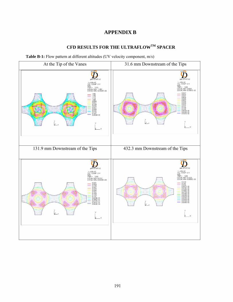
APPENDIX B

CFD RESULTS FOR THE UL TM SPACER

Table B-1: Flow pattern at different altitudes (UV velocity component, m/s)

At the Tip of the Vanes 31.6 mm Downstream of the Tips

TRAFLOW

131.9 mm Downstream of the Tips 432.3 mm Downstream of the Tips

191

Table B-2: Temperature distribution at different altitudes (in Kelvin)

f the VaAt the Tip o nes

131.9 432.3mm Downstream of the Tips mm Downstream of the Tips

192

Table B-3: Turbulent viscosity at different alt

At the Tip of the Vanes

itudes (in Pa-s)

31.6 mm Downstream of the Tips

13 wnstream of the Tips 432.3 mm Downstream of the Tips 1.9 mm Do

193

APPENDIX C

OEFFICIENT MULTIPLIER

ble C-1: Description of the format of the additional input deck with the CFD data for the mixing

Description

CFD DATA FOR THE MIXING C

Tamultiplier

Input Variable N1 – number of entrees for the 1 st independent Total number of axial positions variable N2 – number of entrees for the 2nd independent Total number of different mixing vane

angles variable N3 – number of entrees for the 3 rd independent Dummy variables N4 – number of entrees for the 4 th independent Dummy variables NSET – number of data sets to be read Corresponds to the number of different

subchannel configurations N2_1 – 1 entree of the 2 independenst nd t variable 1st value of the vane angle N2_n – n entree of the 2 independenth nd t variable nth value of the vane angle V_N1 – entree of the independent variable N1 ith axial position V_Nn_1 – value of the dependent variable at a Spacer multiplier for the 1st vane angle

at the ith axial position given combination of N1 and Nn_1 V_Nn_n – value of the dependent variable at a Spacer multiplier for the nth vane angle

at the ith axial position given combination of N1 and Nn_n

194

Table C-2: Example for the CFD data set for the 2×1 case

******

****** N4 0

750 1.032 1.246 1.342 1.267 1.349 815 1.032 1.246 1.342 1.267 1.349

0.845 0.819 1.232 1.679 1.568 1.604 0.875 1.042 1.295 1.322 1.358 1.565 0.905 1.143 0.864 0.959 1.056 1.214 0.935 0.969 0.945 1.399 1.364 1.674 0.965 0.951 1.183 1.470 1.350 1.719 0.995 1.035 1.170 1.298 1.218 1.518 1.025 1.129 1.123 1.182 1.114 1.370 1.055 1.174 1.106 1.157 1.075 1.338 1.085 1.175 1.115 1.174 1.096 1.342 1.115 1.155 1.135 1.197 1.131 1.339 1.145 1.131 1.157 1.218 1.158 1.333 1.175 1.108 1.177 1.239 1.179 1.330 1.205 1.087 1.195 1.258 1.200 1.329 1.235 1.066 1.214 1.279 1.221 1.333 1.265 1.048 1.231 1.304 1.243 1.342 1.295 1.032 1.246 1.342 1.267 1.349 1.360 1.032 1.246 1.342 1.267 1.349 1.390 0.819 1.232 1.679 1.568 1.604 1.420 1.042 1.295 1.322 1.358 1.565 1.450 1.143 0.864 0.959 1.056 1.214 1.480 0.969 0.945 1.399 1.364 1.674 1.510 0.951 1.183 1.470 1.350 1.719 1.540 1.035 1.170 1.298 1.218 1.518 1.570 1.129 1.123 1.182 1.114 1.370 1.600 1.174 1.106 1.157 1.075 1.338 1.630 1.175 1.115 1.174 1.096 1.342 1.660 1.155 1.135 1.197 1.131 1.339 1.690 1.131 1.157 1.218 1.158 1.333 1.720 1.108 1.177 1.239 1.179 1.330 1.750 1.087 1.195 1.258 1.200 1.329 1.780 1.066 1.214 1.279 1.221 1.333 1.810 1.048 1.231 1.304 1.243 1.342 1.840 1.032 1.246 1.342 1.267 1.349

*********************************************** 2D table for the spacer multiplier *********************************************** N1 N2 N3 89 5 0 * NSET 1 * N2_1 N2_2 N2_3 N2_4 N2_5 0.0 10.0 20.0 30.0 50.0 * V_N1 V_N2_1 V_N2_2 V_N2_3 V_N2_4 V_N2_5 0.000 1.000 1.000 1.000 1.000 1.000 0.225 1.000 1.000 1.000 1.000 1.000 0.240 1.032 1.246 1.342 1.267 1.349 0.270 1.032 1.246 1.342 1.267 1.349 0.300 0.819 1.232 1.679 1.568 1.604 0.330 1.042 1.295 1.322 1.358 1.565 0.360 1.143 0.864 0.959 1.056 1.214 0.390 0.969 0.945 1.399 1.364 1.674 0.420 0.951 1.183 1.470 1.350 1.719 0.450 1.035 1.170 1.298 1.218 1.518 0.480 1.129 1.123 1.182 1.114 1.370 0.510 1.174 1.106 1.157 1.075 1.338 0.540 1.175 1.115 1.174 1.096 1.342 0.570 1.155 1.135 1.197 1.131 1.339 0.600 1.131 1.157 1.218 1.158 1.333 0.630 1.108 1.177 1.239 1.179 1.330 0.660 1.087 1.195 1.258 1.200 1.329 0.690 1.066 1.214 1.279 1.221 1.333 0.720 1.048 1.231 1.304 1.243 1.342 0.0.

195

1.905 1.032 1.246 1.342 1.267 1.349

995 1.143 0.864 0.959 1.056 1.214

1.155 1.135 1.197 1.131 1.339 .218 1.158 1.333 .239 1.179 1.330 .258 1.200 1.329 .279 1.221 1.333 .304 1.243 1.342 .342 1.267 1.349 .342 1.267 1.349 .679 1.568 1.604 .322 1.358 1.565 .959 1.056 1.214 .399 1.364 1.674 .470 1.350 1.719 .298 1.218 1.518 .182 1.114 1.370 .157 1.075 1.338 .174 1.096 1.342 .197 1.131 1.339 .218 1.158 1.333 .239 1.179 1.330 .258 1.200 1.329 .279 1.221 1.333 .304 1.243 1.342 .342 1.267 1.349 .342 1.267 1.349

1.935 0.819 1.232 1.679 1.568 1.604 1.965 1.042 1.295 1.322 1.358 1.565 1.2.025 0.969 0.945 1.399 1.364 1.674

1.719 2.055 0.951 1.183 1.470 1.350 2.085 1.035 1.170 1.298 1.218 1.518 2.115 1.129 1.123 1.182 1.114 1.370 2.145 1.174 1.106 1.157 1.075 1.338

1.175 1.115 1.174 1.096 1.342 2.175 5 2.20

2.235 1.131 1.157 12.265 1.108 1.177 1

295 1.087 1.195 12.2.325 1.066 1.214 1

355 1.048 1.231 12.2.385 1.032 1.246 12.450 1.032 1.246 12.480 0.819 1.232 12.510 1.042 1.295 12.540 1.143 0.864 02.570 0.969 0.945 12.600 0.951 1.183 12.630 1.035 1.170 12.660 1.129 1.123 12.690 1.174 1.106 12.720 1.175 1.115 12.750 1.155 1.135 12.780 1.131 1.157 12.810 1.108 1.177 12.840 1.087 1.195 12.870 1.066 1.214 12.900 1.048 1.231 12.930 1.032 1.246 13.000 1.032 1.246 1

196

Table C-3: Example for the CFD data set for ULTRAFLOWTM spacer

**************************** r multiplier **************************** N2 N3 N4 2 0 0

.5347 1.0000 4.0587

.5647 1.0000 2.7668

.5947 1.0000 1.7056

.6247 1.0000 1.1480 1.6547 1.0000 0.9104 1.6847 1.0000 0.8245 1.7147 1.0000 0.8078 1.7447 1.0000 0.8212 1.7747 1.0000 0.8463 1.8047 1.0000 0.8747 1.8347 1.0000 0.9037 1.8647 1.0000 0.9330 1.8947 1.0000 0.9627 1.9247 1.0000 1.0032 1.9867 1.0000 1.0032 2.0167 1.0000 1.1260 2.0467 1.0000 4.0587 2.0767 1.0000 2.7668 2.1067 1.0000 1.7056

************************* 2D table for the space************************* N1 105 * NSET 1 * N2_1 N2_2 0.0 15.0 * * V_N1 V_N2_1 V_N2_2 * 0.0000 1.0000 1.0000 0.4507 1.0000 1.0000 0.4807 1.0000 1.1260 0.5107 1.0000 4.0587 0.5407 1.0000 2.7668 0.5707 1.0000 1.7056 0.6007 1.0000 1.1480 0.6307 1.0000 0.9104 0.6607 1.0000 0.8245 0.6907 1.0000 0.8078 0.7207 1.0000 0.8212 0.7507 1.0000 0.8463 0.7807 1.0000 0.8747 0.8107 1.0000 0.9037 0.8407 1.0000 0.9330 0.8707 1.0000 0.9627 0.9007 1.0000 1.0032 0.9627 1.0000 1.0032 0.9927 1.0000 1.1260 1.0227 1.0000 4.0587 1.0527 1.0000 2.7668 1.0827 1.0000 1.7056 1.1127 1.0000 1.1480 1.1427 1.0000 0.9104 1.1727 1.0000 0.8245 1.2027 1.0000 0.8078 1.2327 1.0000 0.8212 1.2627 1.0000 0.8463 1.2927 1.0000 0.8747 1.3227 1.0000 0.9037 1.3527 1.0000 0.9330 1.3827 1.0000 0.9627 1.4127 1.0000 1.0032 1.4747 1.0000 1.0032 1.5047 1.0000 1.1260 1111

197

2.1367 1.0000 1.1480 2.1667 1.0000 0.9104 2.1967 1.0000 0.8245 2.2267 1.0000 0.8078 2.2567 1.0000 0.8212 2.2867 1.0000 0.8463 2.3167 1.0000 0.8747 2.3467 1.0000 0.9037 2.3767 1.0000 0.9330 2.4067 1.0000 0.9627 2.4367 1.0000 1.0032 2.4987 1.0000 1.0032 2.5287 1.0000 1.1260 2.5587 1.0000 4.0587 2.5887 1.0000 2.7668 2.6187 1.0000 1.7056 2.6487 1.0000 1.1480 2.6787 1.0000 0.9104 2.7087 1.0000 0.8245 2.7387 1.0000 0.8078 2.7687 1.0000 0.8212 2.7987 1.0000 0.8463 2.8287 1.0000 0.8747 2.8587 1.0000 0.9037 2.8887 1.0000 0.9330 2.9187 1.0000 0.9627 2.9487 1.0000 1.0032 3.0107 1.0000 1.0032 3.0407 1.0000 1.1260 3.0707 1.0000 4.0587 3.1007 1.0000 2.7668 3.1307 1.0000 1.7056 3.1607 1.0000 1.1480 3.1907 1.0000 0.9104 3.2207 1.0000 0.8245 3.2507 1.0000 0.8078 3.2807 1.0000 0.8212 3.3107 1.0000 0.8463 3.3407 1.0000 0.8747 3.3707 1.0000 0.9037 3.4007 1.0000 0.9330 3.4307 1.0000 0.9627 3.4607 1.0000 1.0032 3.52273.55273.5827 1.0000 4.0587 3.6127 1.0000 2.7668 3.6427 1.0000 1.7056 3.6727 1.0000 1.1480 3.7027 1.0000 0.9104 3.7080 1.0000 0.8245

1.0000 1.0032 1.0000 1.1260

198

Spacer Grid Multiplier Θ SG

test_sg_mult.out

VDRIFT

SG_MULTIPLIER

Reads the CFD dsg_mult_data

olation subroutine Defines the spacer grid multiplier for the mixing coefficient

multiplier in an additional output file

ata set – input file

Calls the interp

Writes the evaluated spacer grid

test_sg_mult.out

IXFLOW = 2 or 3

YES

Axial height of the F-COBRA-TF momentum cell and Mixing vanes’ angle

Spacer grid multiplier for the given height and angle as defined after linear

Interpolation SubroutinePerforms linear interpolation between values given in the CFD data set

XSCHEM XSCHEM – solves F-COBRA-TF conservation equations

r modeling of the enhanced turbulent mixing and directed crossflow

IXFLOW = 2 – only enhanced turbulent mixing modeling will be activated;

IXFLOW = 3 – both modeling options will be activated

SG_MULTIPLIER – evaluates spacer grid

VDRIFT – calculates turbulent mixing and void drift source terms

IXFLOW – input flag fo

multiplier ΘSG

test_sg_mult

ced ixFigure C-1: Flow chart of the modeling of the enhan turbulent m ing due to mixing vanes

199

APPENDIX D

EVALUATION OF THE TPREDICTIONS FOR THE VELOCITY CURL

andidate 1:

RANSVERSE MOMENTUM CHANGE BY MEANS OF CFD

C

the velocity curl in a lateral plane, Knowing

⎟⎟⎠

⎞⎜⎛ ∂∂ vv yzr⎜⎝ ∂

−∂

==×∇zy

vcurlvx

)( , (A.1)

a body force can be calculated as

xAvvF x ∆×∇= ρ)( , (A.2)

where xv is the xial velocity in the fluid do ain and a m ρ is its density as both calculated by F-

COBRA-TF, A is the area on which the force is acting and x∆ is the axial dimension of the

domain for a particular case.

We can assume that the area A is equal to , where 2RA π= R is the distance between the

center of the subchannel and the rod surface (see Figure D-1).

R

Figure D-1: Schematic of the model for evaluation of the lateral momentum change by velocity curl

200

The momentum change I& in the latera time interval is then defined as: l direction y over a t∆

xA ∆ρ . vvFtII xlat ×∇=≡

∆∆

= )(& (A.3)

Candidate 2:

The pressure gradient over the radius R in Figure D-1 can be given as

32143421 gravity

force lcentrofuga

22

21 hgRP ρρω +=∆ (A.4)

where ρ is the density of the medium; R is the distance between the center of the subchannel and

the rod surface; ω is the angular velocity; and g is the gravitational constant.

sing the relaNeglecting the gravity term and u tion between the angular velocity ω and the

velocity curl, 4

)( v×∇=ω , the pressure gradient becomes

2222 )(81

21 RvRP ×∇==∆ ρρω , (A.5)

Then the lateral momentum change by the force acting on the fluid at the gap area (lateral area

, where is the rod-to-rod distance) due to the pressure gradient xSA ijlat ∆= ijS P∆ will be

xSRvAPFtII ijlatlat ∆×∇=∆=≡∆∆

= 22)(81 ρ& . (A.6)

201

APPENDIX E

CFD RESULTS FOR THE FOCUSTM SPACER

Table E-1: Lateral (UW) velocities field immediately downstream of the mixing vanes

10 degree, local maximum of 0.9245 m/s 20 degree, local maximum of 1.782 m/s

30 degree, local maximum of 2.483 m/s 40 degree, local maximum of 2.846 m/s

202

Table E-2: Lateral velocity field further downstream of the spacer

20 degree 0.330 m

30 degree 0.330 m

40 degree 0.430 m

203

Table E-3: Lateral velocities field at the position of ‘velocity inversion’ 20 degree 0.375 m

30 degree 0.395 m

40 degree 0.445 m

204

UW Velocity10 degree

-0,4

-0,3

-0,2

-0,1

0,0

0,1

0,2

0,3

0,4

0 100 200 300 400 500 600

Height, mm

Velo

city

, m/s north

southwesteast

north

southeastwest

Figure E-1: Axial distribution of the lateral (UW) velocity for FOCUSTM spacer with mixing vanes of 10°


-1,00

-0,80

-0,60

-0,40

-0,20

0,00

0,20

0,40

0,60

0,80

1,00

0 100 200 300 400 500 600

Height, mm

Vel

ocity

, m/s east

westnortsouth

north

southeastwest


205


-0,5

0,5

1,0

1,5

Velo

/s east

0,0

city

, m west

-1,5

-1,0

0 100 200 300 400 500

Height, mm

600

southnorth

north

southeastwest

Figur ixing vanes of 30°

e E-3: Axial distribution of the lateral (UW) velocity for FOCUSTM spacer with m


-2,00

-1,50

0

Height, mm

Vel

ocity

, m/s

-1,00

-0,500 100 200 300 400 5

0,00

0,50

1,00

1,50

2,00

0 600

eastwestnorthsouth

north


southeastwest

206

ONVECTION FACTOR

at of the additional input deck with the CFD data for the lateral

Description

APPENDIX F

CFD DATA FOR THE LATERAL C

Table F-1: Description of the formconvection factor

Input Variable N1 – number of entrees for the 1st independent Total number of axial positions variable N2 – number of entrees for the 2nd independent Total number of different mixing vane

angles variable N3 – number of entrees for the 3rd independent Dummy variables N4 – number of entrees for the 4th independent Dummy variables NSET – number of data sets to be read Corresponds to the number of different

subchannel configurations N2_1 – 1 entree of the 2 indst nd ependent variable 1st value of the vane angle N2_n – n entree of the 2 indth nd ependent variable nth value of the vane angle V_N1 – entree of the independent variable N1 ith axial position V_Nn_1 – value of the dependent variable at a

n_1 Spacer multiplier for the 1st vane angle at the ith axial position given combination of N1 and N

V_Nn_n – value of the dependent variable at a n_n

Spacer multiplier for the nth vane angle at the ith axial position given combination of N1 and N

207

Table F-2: Example for the CFD data set for the FOCUSTM spacer ************** or ************** N3 N4 0 0

*************************************** 2D table for lateral convection fact*************************************** N1 N2 260 4 * NSET 1 * N2_1 N2_2 N2_3 N2_4 10.0 20.0 30.0 40.0 * V_N1 V_N2_1 V_N2_2 V_N2_3 V_N2_4 0.00 0.0000 0.0000 0.0000 0.0000 0.23 0.0001 0.0001 0.0001 0.0001 0.24 0.0001 0.0001 0.0001 0.0001 0.25 0.0001 0.0001 0.0001 0.0001 0.26 0.0001 0.0001 0.0001 0.0001 0.27 0.0002 0.0002 0.0002 0.0002 0.28 0.0002 0.0002 0.0002 0.0002 0.29 0.0001 0.0001 0.0001 0.0001 0.30 0.0001 0.0001 0.0001 0.0001 0.31 0.0012 0.0026 0.0033 0.0039 0.32 0.0139 0.0430 0.0839 0.1282 0.33 0.0282 0.1198 0.2012 0.2689 0.34 0.0396 0.1496 0.2517 0.3428 0.35 0.0480 0.1693 0.2756 0.3473 0.36 0.0537 0.1763 0.2629 0.3265 0.37 0.0575 0.1667 0.2421 0.3117 0.38 0.0605 0.1499 0.2262 0.2912 0.39 0.0630 0.1327 0.2086 0.2620 0.40 0.0647 0.1186 0.1867 0.2325 0.41 0.0652 0.1076 0.1654 0.2068 0.42 0.0645 0.0982 0.1486 0.1837 0.43 0.0630 0.0900 0.1367 0.1646 0.44 0.0610 0.0832 0.1278 0.1512 0.45 0.0586 0.0782 0.1208 0.1432 0.46 0.0563 0.0749 0.1154 0.1383 0.47 0.0538 0.0725 0.1108 0.1341 0.48 0.0514 0.0707 0.1070 0.1303 0.49 0.0493 0.0692 0.1038 0.1272 0.50 0.0472 0.0674 0.1008 0.1244 0.51 0.0454 0.0655 0.0980 0.1221 0.52 0.0439 0.0636 0.0958 0.1202 0.53 0.0424 0.0615 0.0937 0.1184 0.54 0.0411 0.0594 0.0919 0.1167 0.55 0.0399 0.0575 0.0903 0.1152 0.56 0.0387 0.0555 0.0888 0.1136 0.57 0.0375 0.0535 0.0872 0.1119 0.58 0.0365 0.0515 0.0856 0.1100 0.59 0.0354 0.0494 0.0836 0.1077 0.60 0.0344 0.0491 0.0814 0.1049 0.61 0.0335 0.0506 0.0788 0.1019 0.62 0.0326 0.0531 0.0765 0.0981 0.63 0.0317 0.0552 0.0761 0.0938 0.64 0.0309 0.0568 0.0753 0.0892 0.65 0.0302 0.0581 0.0740 0.0836 0.66 0.0295 0.0589 0.0721 0.0774 0.67 0.0289 0.0593 0.0699 0.0720 0.68 0.0283 0.0593 0.0669 0.0694 0.69 0.0277 0.0589 0.0643 0.0667 0.70 0.0272 0.0582 0.0641 0.0658 0.71 0.0267 0.0572 0.0637 0.0659 0.72 0.0261 0.0560 0.0632 0.0658 0.73 0.0256 0.0547 0.0625 0.0656 0.74 0.0250 0.0533 0.0617 0.0652 0.75 0.0244 0.0519 0.0608 0.0646 0.76 0.0238 0.0509 0.0596 0.0638 0.83 0.0238 0.0509 0.0596 0.0638

208

0.84 0.0238 0.0509 0.0596 0.0638 0.85 0.0238 0.0509 0.0596 0.0638 0.86 0.0238 0.0509 0.0596 0.0638 0.87 0.0238 0.0509 0.0596 0.0638 0.88 0.0238 0.0509 0.0596 0.0638 0.89 0.0282 0.1198 0.2012 0.2689 0.90 0.0396 0.1496 0.2517 0.3428 0.91 0.0480 0.1693 0.2756 0.3473 0.92 0.0537 0.1763 0.2629 0.3265 0.93 0.0575 0.1667 0.2421 0.3117 0.94 0.0605 0.1499 0.2262 0.2912 0.95 0.0630 0.1327 0.2086 0.2620 0.96 0.0647 0.1186 0.1867 0.2325 0.97 0.0652 0.1076 0.1654 0.2068 0.98 0.0645 0.0982 0.1486 0.1837 0.99 0.0630 0.0900 0.1367 0.1646 1.00 0.0610 0.0832 0.1278 0.1512 1.01 0.0586 0.0782 0.1208 0.1432 1.02 0.0563 0.0749 0.1154 0.1383 1.03 0.0538 0.0725 0.1108 0.1341 1.04 0.0514 0.0707 0.1070 0.1303 1.05 0.0493 0.0692 0.1038 0.1272 1.06 0.0472 0.0674 0.1008 0.1244 1.07 0.0454 0.0655 0.0980 0.1221 1.08 0.0439 0.0636 0.0958 0.1202 1.09 0.0424 0.0615 0.0937 0.1184 1.10 0.0411 0.0594 0.0919 0.1167 1.11 0.0399 0.0575 0.0903 0.1152 1.12 0.0387 0.0555 0.0888 0.1136 1.13 0.0375 0.0535 0.0872 0.1119 1.14 0.0365 0.0515 0.0856 0.1100 1.15 0.0354 0.0494 0.0836 0.1077 1.16 0.0344 0.0491 0.0814 0.1049 1.17 0.0335 0.0506 0.0788 0.1019 1.18 0.0326 0.0531 0.0765 0.0981 1.19 0.0317 0.0552 0.0761 0.0938 1.20 0.0309 0.0568 0.0753 0.0892 1.21 0.0302 0.0581 0.0740 0.0836 1.22 0.0295 0.0589 0.0721 0.0774 1.23 0.0289 0.0593 0.0699 0.0720 1.24 0.0283 0.0593 0.0669 0.0694 1.25 0.0277 0.0589 0.0643 0.0667 1.26 0.0272 0.0582 0.0641 0.0658 1.27 0.0267 0.0572 0.0637 0.0659 1.28 0.0261 0.0560 0.0632 0.0658 1.29 0.0256 0.0547 0.0625 0.0656 1.30 0.0250 0.0533 0.0617 0.0652 1.31 0.0244 0.0519 0.0608 0.0646 1.32 0.0238 0.0509 0.0596 0.0638 1.37 0.0238 0.0509 0.0596 0.0638 1.38 0.0238 0.0509 0.0596 0.0638 1.39 0.0238 0.0509 0.0596 0.0638 1.40 0.0238 0.0509 0.0596 0.0638 1.41 0.0238 0.0509 0.0596 0.0638 1.42 0.0238 0.0509 0.0596 0.0638 1.43 0.0282 0.1198 0.2012 0.2689 1.44 0.0396 0.1496 0.2517 0.3428 1.45 0.0480 0.1693 0.2756 0.3473 1.46 0.0537 0.1763 0.2629 0.3265 1.47 0.0575 0.1667 0.2421 0.3117 1.48 0.0605 0.1499 0.2262 0.2912 1.49 0.0630 0.1327 0.2086 0.2620 1.50 0.0647 0.1186 0.1867 0.2325 1.51 0.0652 0.1076 0.1654 0.2068 1.52 0.0645 0.0982 0.1486 0.1837 1.53 0.0630 0.0900 0.1367 0.1646 1.54 0.0610 0.0832 0.1278 0.1512 1.55 0.0586 0.0782 0.1208 0.1432 1.56 0.0563 0.0749 0.1154 0.1383 1.57 0.0538 0.0725 0.1108 0.1341 1.58 0.0514 0.0707 0.1070 0.1303

209

1.59 0.0493 0.0692 0.1038 0.1272 1.60 0.0472 0.0674 0.1008 0.1244 1.61 0.0454 0.0655 0.0980 0.1221 1.62 0.0439 0.0636 0.0958 0.1202 1.63 0.0424 0.0615 0.0937 0.1184 1.64 0.0411 0.0594 0.0919 0.1167 1.65 0.0399 0.0575 0.0903 0.1152 1.66 0.0387 0.0555 0.0888 0.1136 1.67 0.0375 0.0535 0.0872 0.1119 1.68 0.0365 0.0515 0.0856 0.1100 1.69 0.0354 0.0494 0.0836 0.1077 1.70 0.0344 0.0491 0.0814 0.1049 1.71 0.0335 0.0506 0.0788 0.1019 1.72 0.0326 0.0531 0.0765 0.0981 1.73 0.0317 0.0552 0.0761 0.0938 1.74 0.0309 0.0568 0.0753 0.0892 1.75 0.0302 0.0581 0.0740 0.0836 1.76 0.0295 0.0589 0.0721 0.0774 1.77 0.0289 0.0593 0.0699 0.0720 1.78 0.0283 0.0593 0.0669 0.0694 1.79 0.0277 0.0589 0.0643 0.0667 1.80 0.0272 0.0582 0.0641 0.0658 1.81 0.0267 0.0572 0.0637 0.0659 1.82 0.0261 0.0560 0.0632 0.0658 1.83 0.0256 0.0547 0.0625 0.0656 1.84 0.0250 0.0533 0.0617 0.0652 1.85 0.0244 0.0519 0.0608 0.0646 1.86 0.0238 0.0509 0.0596 0.0638 1.92 0.0238 0.0509 0.0596 0.0638 1.93 0.0238 0.0509 0.0596 0.0638 1.94 0.0238 0.0509 0.0596 0.0638 1.95 0.0238 0.0509 0.0596 0.0638 1.96 0.0238 0.0509 0.0596 0.0638 1.97 0.0238 0.0509 0.0596 0.0638 1.98 0.0282 0.1198 0.2012 0.2689 1.99 0.0396 0.1496 0.2517 0.3428 2.00 0.0480 0.1693 0.2756 0.3473 2.01 0.0537 0.1763 0.2629 0.3265 2.02 0.0575 0.1667 0.2421 0.3117 2.03 0.0605 0.1499 0.2262 0.2912 2.04 0.0630 0.1327 0.2086 0.2620 2.05 0.0647 0.1186 0.1867 0.2325 2.06 0.0652 0.1076 0.1654 0.2068 2.07 0.0645 0.0982 0.1486 0.1837 2.08 0.0630 0.0900 0.1367 0.1646 2.09 0.0610 0.0832 0.1278 0.1512 2.10 0.0586 0.0782 0.1208 0.1432 2.11 0.0563 0.0749 0.1154 0.1383 2.12 0.0538 0.0725 0.1108 0.1341 2.13 0.0514 0.0707 0.1070 0.1303 2.14 0.0493 0.0692 0.1038 0.1272 2.15 0.0472 0.0674 0.1008 0.1244 2.16 0.0454 0.0655 0.0980 0.1221 2.17 0.0439 0.0636 0.0958 0.1202 2.18 0.0424 0.0615 0.0937 0.1184 2.19 0.0411 0.0594 0.0919 0.1167 2.20 0.0399 0.0575 0.0903 0.1152 2.21 0.0387 0.0555 0.0888 0.1136 2.22 0.0375 0.0535 0.0872 0.1119 2.23 0.0365 0.0515 0.0856 0.1100 2.23 0.0354 0.0494 0.0836 0.1077 2.24 0.0344 0.0491 0.0814 0.1049 2.25 0.0335 0.0506 0.0788 0.1019 2.26 0.0326 0.0531 0.0765 0.0981 2.27 0.0317 0.0552 0.0761 0.0938 2.28 0.0309 0.0568 0.0753 0.0892 2.29 0.0302 0.0581 0.0740 0.0836 2.30 0.0295 0.0589 0.0721 0.0774 2.31 0.0289 0.0593 0.0699 0.0720 2.32 0.0283 0.0593 0.0669 0.0694 2.33 0.0277 0.0589 0.0643 0.0667

210

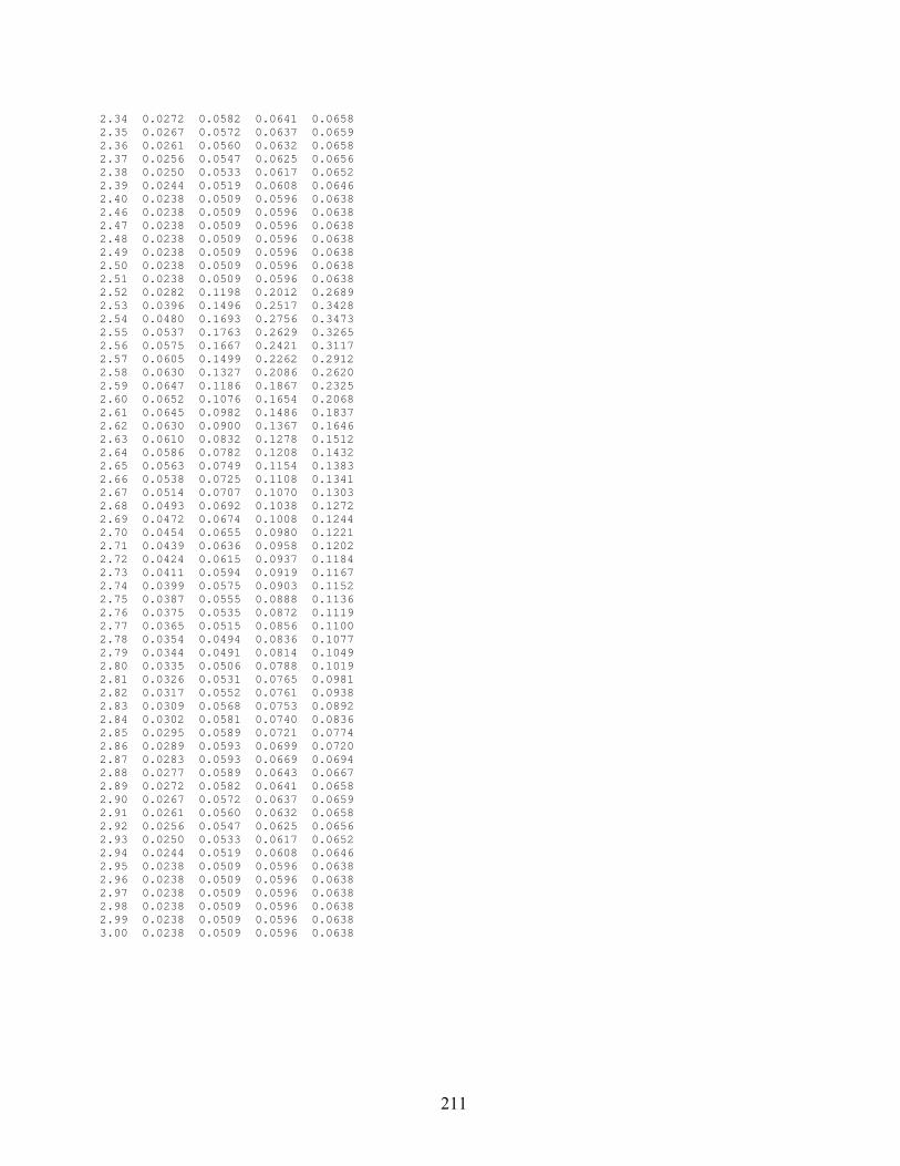
2.34 0.0272 0.0582 0.0641 0.0658 2.35 0.0267 0.0572 0.0637 0.0659 2.36 0.0261 0.0560 0.0632 0.0658 2.37 0.0256 0.0547 0.0625 0.0656 2.38 0.0250 0.0533 0.0617 0.0652 2.39 0.0244 0.0519 0.0608 0.0646 2.40 0.0238 0.0509 0.0596 0.0638 2.46 0.0238 0.0509 0.0596 0.0638 2.47 0.0238 0.0509 0.0596 0.0638 2.48 0.0238 0.0509 0.0596 0.0638 2.49 0.0238 0.0509 0.0596 0.0638 2.50 0.0238 0.0509 0.0596 0.0638 2.51 0.0238 0.0509 0.0596 0.0638 2.52 0.0282 0.1198 0.2012 0.2689 2.53 0.0396 0.1496 0.2517 0.3428 2.54 0.0480 0.1693 0.2756 0.3473 2.55 0.0537 0.1763 0.2629 0.3265 2.56 0.0575 0.1667 0.2421 0.3117 2.57 0.0605 0.1499 0.2262 0.2912 2.58 0.0630 0.1327 0.2086 0.2620 2.59 0.0647 0.1186 0.1867 0.2325 2.60 0.0652 0.1076 0.1654 0.2068 2.61 0.0645 0.0982 0.1486 0.1837 2.62 0.0630 0.0900 0.1367 0.1646 2.63 0.0610 0.0832 0.1278 0.1512 2.64 0.0586 0.0782 0.1208 0.1432 2.65 0.0563 0.0749 0.1154 0.1383 2.66 0.0538 0.0725 0.1108 0.1341 2.67 0.0514 0.0707 0.1070 0.1303 2.68 0.0493 0.0692 0.1038 0.1272 2.69 0.0472 0.0674 0.1008 0.1244 2.70 0.0454 0.0655 0.0980 0.1221 2.71 0.0439 0.0636 0.0958 0.1202 2.72 0.0424 0.0615 0.0937 0.1184 2.73 0.0411 0.0594 0.0919 0.1167 2.74 0.0399 0.0575 0.0903 0.1152 2.75 0.0387 0.0555 0.0888 0.1136 2.76 0.0375 0.0535 0.0872 0.1119 2.77 0.0365 0.0515 0.0856 0.1100 2.78 0.0354 0.0494 0.0836 0.1077 2.79 0.0344 0.0491 0.0814 0.1049 2.80 0.0335 0.0506 0.0788 0.1019 2.81 0.0326 0.0531 0.0765 0.0981 2.82 0.0317 0.0552 0.0761 0.0938 2.83 0.0309 0.0568 0.0753 0.0892 2.84 0.0302 0.0581 0.0740 0.0836 2.85 0.0295 0.0589 0.0721 0.0774 2.86 0.0289 0.0593 0.0699 0.0720 2.87 0.0283 0.0593 0.0669 0.0694 2.88 0.0277 0.0589 0.0643 0.0667 2.89 0.0272 0.0582 0.0641 0.0658 2.90 0.0267 0.0572 0.0637 0.0659 2.91 0.0261 0.0560 0.0632 0.0658 2.92 0.0256 0.0547 0.0625 0.0656 2.93 0.0250 0.0533 0.0617 0.0652 2.94 0.0244 0.0519 0.0608 0.0646 2.95 0.0238 0.0509 0.0596 0.0638 2.96 0.0238 0.0509 0.0596 0.0638 2.97 0.0238 0.0509 0.0596 0.0638 2.98 0.0238 0.0509 0.0596 0.0638 2.99 0.0238 0.0509 0.0596 0.0638 3.00 0.0238 0.0509 0.0596 0.0638

211

212

DIRECTED_CROSSFLOW Reads input data for orientation of directed crossflows Calls XFLOW to define the lateral convection factor Evaluates the force to be added as a source term to the lateral momentum equation

IXFLOW = 1 or 3

YES

XFLOW Reads the CFD data set – input file xflow_data Calls the interpolation subroutine Writes the evaluated lateral convection factor in an additional output file test_xlow.out

Axial height of the F-COBRA-TF momentum cell and Mixing vanes’ angle

Lateral convection factor for the given height and angle as interpolated by LINT4D

Source term Flat_conv_sg

test_xflow.out

xflow_data

Interpolation SubroutinePerforms linear interpolation between values given in the CFD data set

dirct_data_inp

XSCHEM XSCHEM – solves F-COBRA-TF conservation equations

DIRECTED_CROSSFLOW – calculates the source term Flat_conv_sg

IXFLOW – input flag for modeling of the enhanced turbulent mixing and directed crossflow

IXFLOW = 1 – only directed crossflow modeling will be activated;

IXFLOW = 3 – both modeling options will be activated

Figure F-1: Flow chart of the modeling of the directed crossflow

Vita

Maria Avramova was born in Zlatograd, Bulgaria on August 21, 1968. Maria received her M.S.

degree in Nuclear Technique and Nuclear Energy from the Sofia University “St. Kliment

Ohridski”, Sofia, Bulgaria in December of 1993. She started her job as a physicist in the

Department of Thermal-Hydraulics and Reactor Safety of the Institute for Nuclear Research and

Nuclear Energy, Bulgarian Academy of Science, Sofia, Bulgaria on October 1994. Maria began

post graduate studies in Nuclear Engineering at the Pennsylvania State University in January,

2001, where she received her M.S. in August, 2003. Maria Avramova continued her study at the

Pennsylvania State University and earned her Ph.D. degree in Nuclear Engineering in December,

2007.

Documents

DEVELOPMENT OF AN INNOVATIVE SPACER GRID MODEL …