Embed Size (px)
Citation preview

MASTER PROGRAM IN
INTERNATIONAL STUDY IN
PETROLEUM ENGINEERING
Development of an Energy Consumption Model
Based on Standard Drilling Parameters
Dipl. Ing. Gabriel Gomes Müller
Leoben, June 2015
Chair of Drilling and Completion Engineering
ii
UNIVERSITY OF LEOBEN
MASTER PROGRAM IN
INTERNATIONAL STUDY IN
PETROLEUM ENGINEERING
Development of an Energy Consumption Model
Based on Standard Drilling Parameters
Master Thesis submitted to the Master Program in International Study in Petroleum Engineering as partial fulfillment of the requirements for the title award Master of Science (M.Sc.) in International Study in Petroleum Engineering.
Degree emphasis module: Drilling Engineering
Supervisor: Univ.-Prof. Dipl.-Ing. Dr.mont. Gerhard Thonhauser
Co-supervisor: Prof. Dr. Edson da Costa Bortoni
June 2015

Chair of Drilling and Completion Engineering
iii
DEDICATORY
This thesis is dedicated to my parents who have supported me all the way since the
beginning of my studies.
Also, this thesis is dedicated to Elena who has been a great source of motivation and
inspiration.
Finally, this thesis is dedicated to all those who believe in the richness of learning.
“There are men who
struggle for a day, and
they are good. There are
others who struggle for a
year, and they are better.
There are some who
struggle many years, and
they are better still.
But there are those who
struggle all their lives, and
these are the
indispensable ones.”
Bertolt Brecht

Chair of Drilling and Completion Engineering
iv
Affidavit
I declare in lieu of oath, that I wrote this thesis myself and have not used any sources other
than quoted at the end of the thesis. This Master Thesis has not been submitted elsewhere
for examination purpose.
Ich erkläre hiermit Eides statt, die vorliegende Arbeit eigenhändig, lediglich unter
Verwendung der zitierten Literatur angefertigt zu haben. Diese Diplomarbeit wurde nirgends
sonst zur Beurteilung eingereicht.
Leoben, June 28, 2015
_______________________
(Gabriel Gomes Müller)

Chair of Drilling and Completion Engineering
v
ACKNOWLEDGEMENTS
To Univ.-Prof. Dipl.-Ing.Dr.mont. Gerhard Thonhauser (MUL) and Prof. Dr. Edson da Costa
Bortoni (UNIFEI), for the orientation, guidance, patience, and support while developing this
research.
To Univ.-Prof. Dipl.-Ing.Dr.mont. Herbert Hofstätter, Ass.Prof. Dipl.-Ing. Dr.mont.Michael
Prohaska-Marchried, Dipl.-Ing.Dr.mont. Stefan Wirth from MUL and to Dr. Antonio Claret
Silva Gomes, for all the attention provided over this degree.
To all employees and professors from the University of Leoben (Montanuniversität Leoben,
MUL). To all employees and professors from the Federal University of Itajubá (Universidade
Federal de Itajubá, UNIFEI).
To all friends, especially those from Leoben, for following up and believing in the
development of this work. Thank you very much Elena Chevelcha for your exceptional
support.
To all my colleagues at TDE, who supported me.
To my family, for their help and encouragement in developing this thesis.

Chair of Drilling and Completion Engineering
vi
Abstract
Current lower oil price has thrown energy efficiency into sharp focus. The author believes
that the drilling industry should have a responsibility to minimize cost and maximize efficiency
in all circumstances. The thesis develops methods to quantify energy consumed for drilling
as a potential drilling optimization. For this purpose, energy consumption models are
developed and empirical measurements are made to track performance against the model.
General energy consumption concepts are used to develop three mathematical energy
consumption models for each of the major energy consumers of a rig: mud pumps, top drive
and draw-works. Thesis includes justification and explanation of developed models with
supporting theory. The research also includes a chapter dedicated to models confirmation,
verification and validation, where modeled fuel consumed results are cross referenced
against the real fuel consumed data. These steps gradually prove accuracy of the created
energy consumption models.
As a result, the thesis proves the possibility to use the drilling parameters to accurately
calculate the energy consumption for each phase of rig activity. Thesis also offers to improve
models by enhancing drilling data quality and drilling rig specifications. Additionally, the
author suggests the further application of the research in the area related to drilling energy
efficiency KPIs.

Chair of Drilling and Completion Engineering
vii
LIST OF FIGURES
Figure 1: AC drilling rig with main components ...................................................................... 4
Figure 2: Rotary system ........................................................................................................ 6
Figure 3: Hoisting system schematic ..................................................................................... 8
Figure 4: Draw-works ............................................................................................................ 9
Figure 5: Circulation system .................................................................................................10
Figure 6: Triplex mup pumps ................................................................................................11
Figure 7: Single acting piston schematic...............................................................................11
Figure 8: Schematic variable‐ frequency drive. ....................................................................16
Figure 9: VFD efficiency at full and partial load .....................................................................17
Figure 10: Energy consumption model flow chart. ................................................................20
Figure 11: Energy flow in a rig equipment. ............................................................................24
Figure 12: Variation in losses due to motor loading. .............................................................28
Figure 13: Motor losses by the square of the load of a top drive with the regression line. .....29
Figure 14: Graphic representation of the load vs. efficiency for the VFD. .............................30
Figure 15: Energy flow in a top drive. ...................................................................................31
Figure 16: Energy flow in a mud pump. ................................................................................33
Figure 17: Energy flow in a draw-works. ...............................................................................36
Figure 18: Simplified view of the model CV&V process .......................................................43
Figure 19: Fuel consumption variation by load......................................................................48
Figure 20: Real Fuel vs. Calculated Fuel Consumption referent to the period of 0-12h. ........51
Figure 21: Real Fuel vs. Calculated Fuel Consumption referent to the period of 12-24h. ......51
Figure 22: Real Fuel vs. Calculated Fuel Consumption referent to the period of 0-24h. ........52
Figure 23: Coefficient of determination from real values vs. calculated values. ....................53
Figure 24: General coefficient of determination for the Energy Consumption Model. ............54
Figure 25: Detailed model development and CV&V ..............................................................55

Chair of Drilling and Completion Engineering
viii
LIST OF TABLES
Table 1: Fuel Efficiency Consumption Table .........................................................................15
Table 2: Minimum set of data channels. ...............................................................................20
Table 3: Drilling Data used in the model with 0.2 Hz sampling frequency. ............................21
Table 4: Top drive, mud pumps and draw-works necessary specifications. ..........................23
Table 5: Motor loss categories ..............................................................................................28
Table 6: Top drive calculation results used in the model with 0.2 Hz sampling frequency. ....32
Table 7: Mud pump calculation results used in the model with 0.2 Hz sampling frequency. ..34
Table 8: Draw-works calculation results used in the model with 0.2 Hz sampling frequency. 39
Table 9: Generators input data. ............................................................................................47
Table 10: Drilling data used in the model with 0.2 Hz sampling frequency. ...........................49
Table 11: Real and calculated values of fuel consumed by the rig A. ...................................50

Chair of Drilling and Completion Engineering
ix
LIST OF EQUATIONS
Eq. 1 .....................................................................................................................................23
Eq. 2 .....................................................................................................................................23
Eq. 3 .....................................................................................................................................24
Eq. 4 .....................................................................................................................................25
Eq. 5 .....................................................................................................................................25
Eq. 6 .....................................................................................................................................25
Eq. 7 .....................................................................................................................................26
Eq. 8 .....................................................................................................................................26
Eq. 9 .....................................................................................................................................26
Eq. 10 ...................................................................................................................................29
Eq. 11 ...................................................................................................................................30
Eq. 12 ...................................................................................................................................31
Eq. 13 ...................................................................................................................................32
Eq. 14 ...................................................................................................................................34
Eq. 15 ...................................................................................................................................35
Eq. 16 ...................................................................................................................................35
Eq. 17 ...................................................................................................................................35
Eq. 18 ...................................................................................................................................36
Eq. 19 ...................................................................................................................................37
Eq. 20 ...................................................................................................................................37
Eq. 21 ...................................................................................................................................38
Eq. 22 ...................................................................................................................................38
Eq. 23 ...................................................................................................................................38
Eq. 24 ...................................................................................................................................38
Eq. 25 ...................................................................................................................................39
Eq. 26 ...................................................................................................................................40
Eq. 27 ...................................................................................................................................41
Eq. 28 ...................................................................................................................................41
Eq. 29 ...................................................................................................................................47
Eq. 30 ...................................................................................................................................48
Eq. 31 ...................................................................................................................................48

Chair of Drilling and Completion Engineering
x
CONTENT
Abstract ................................................................................................................................. vi
LIST OF FIGURES ............................................................................................................... vii
LIST OF TABLES ................................................................................................................ viii
LIST OF EQUATIONS ........................................................................................................... ix
CONTENT .............................................................................................................................. x
1. Introduction .................................................................................................................... 1
1.1 Thesis structure ....................................................................................................... 2
2. Drilling Rig System ......................................................................................................... 3
2.1 Drilling Rig ............................................................................................................... 3
2.1.1 AC Drilling Rig .................................................................................................. 4
2.2 Rotary System ......................................................................................................... 5
2.2.1 Top Drive ......................................................................................................... 6
2.2.2 RPM Sensor ..................................................................................................... 7
2.2.3 Torque Sensor ................................................................................................. 7
2.3 Hoisting System ...................................................................................................... 8
2.3.1 Draw-works ...................................................................................................... 8
2.3.2 Hookload Sensor .............................................................................................. 9
2.3.3 Travelling Block Sensor ...................................................................................10
2.4 Circulating System .................................................................................................10
2.4.1 Mud Pumps .....................................................................................................11
2.4.2 Flow Rate Sensor ............................................................................................12
2.4.3 Pump Pressure Sensor ...................................................................................12
2.4.4 Mud Density Sensor ........................................................................................12
2.5 Power System ........................................................................................................13
2.5.1 Diesel Generator .............................................................................................13
2.5.2 Variable Frequency Driver (VFD) Room ..........................................................15
2.6 Other RigSensors ...................................................................................................18
2.6.1 Hole Depth Readings ......................................................................................18
2.6.2 Bit Depth Readings .........................................................................................18
2.6.3 Weight on Bit Readings ...................................................................................18
3. Energy Consumption Mathematical Model ....................................................................19
3.1 Input Data ..............................................................................................................19
3.1.1 Drilling Data Channels .....................................................................................20
3.1.1.1 Drilling Data Quality Control .....................................................................21
3.2 General Energy Consumption Concepts ................................................................23

Chair of Drilling and Completion Engineering
xi
3.2.1 Power Output ..................................................................................................24
3.2.1.1 Mechanical Power ....................................................................................25
3.2.1.2 Hydraulic Power .......................................................................................25
3.2.2 System Losses andEfficiency ..........................................................................26
3.2.2.1 Overall Losses .........................................................................................27
3.2.2.2 Motor Efficiency and Losses.....................................................................27
3.2.2.3 VFD Losses .............................................................................................29
3.3 Energy Consumption Models Description ...............................................................30
3.3.1 Top Drive Energy Consumption Model ............................................................31
3.3.1.1 Top Drive Overall Efficiency .....................................................................33
3.3.2 Mud Pumps Energy Consumption Model ........................................................33
3.3.2.1 Mud Pump Overall Efficiency ...................................................................34
3.3.3 Draw-works Energy Consumption Model .........................................................36
3.3.3.1 Tripping-In Energy Consumption Model ...................................................37
3.3.3.2 Tripping-Out Energy Consumption Model .................................................37
3.3.3.3 Draw-works Overall Efficiency ..................................................................40
3.3.4 Extra Equipment Energy Consumption Model .................................................40
3.3.5 Final Integrated Model .....................................................................................41
4. Model Confirmation, Verification& Validation .................................................................42
4.1 Model Confirmation ................................................................................................44
4.2 Model Verification ...................................................................................................44
4.3 Model Validation .....................................................................................................45
4.3.1 Fuel Consumption Model ................................................................................46
4.3.1.1 Input Data ................................................................................................46
4.3.1.2 Fuel Consumption Model Description .......................................................47
4.3.2 Model Predictions vs. Measured Data .............................................................49
4.3.2.1 Graphical Comparison of Data .................................................................50
4.3.2.2 Coefficient of Determination - R2 ..............................................................52
4.4 Accreditation ..........................................................................................................54
5. Conclusion ....................................................................................................................56
6. Bibliography ..................................................................................................................58
Appendix A– Fuel Consumption Results& Comparison ........................................................61
LIST OF SYMBOLS .............................................................................................................69

Chair of Drilling and Completion Engineering
1
1. Introduction
The climate of drastically dropping oil price reminds to the oil companies that any penny
saved is a penny earned. Due to historical oil price fluctuations the topic of drilling efficiency
became important in terms of determining the commerciality of drilling in field development
activities. The energy consumption is a great contributing factor of the operational drilling
cost as it accounts for 10-30% of the operational cost, thus, energy efficiency of a drilling rig
is a vital point (Cherutich, 2009). Especially, this becomes essential when discussing large
scale field development of unconventional resources, which frequently have high drilling
intensity and an elevated cost per barrel ratio. Thus, the knowledge regarding the energy
required to drill a well, and monitoring of its consumption can improve understanding of the
well profitability and drilling process. Energy efficiency in the drilling phase has the potential
to reduce overall development Capital Expenditure. By using information about energy
required to drill a well, drilling engineers can take leading decisions in terms of type of
equipment to use (e.g. type of drill bits, top drives), rate of penetration (faster may not mean
better), drilling mud pumping rate, among others. Beyond commercial benefits, improved
energy efficiency can also reduce the carbon footprint for development drilling activity. The
considerable message of the thesis is to underline the importance of managing energy
consumption in drilling activities.
The idea of the thesis is to support a PhD student of the University of Leoben
(Montanuniversität Leoben), MSc Mathias Mitschanek, in the research related to the
simulation of the development of large unconventional fields. Thus, the thesis focuses on a
part of this macro model in regards to energy consumed during the well construction phase.
Drilling process can be described with the help of eight drilling parameters, which are
measured at the rig site with the help of sensors (this is shortly mentioned in the thesis) and
are used to calculate Key Performance Indicators (KPIs). KPIs are monitored, recorded and
stored during each phase of the drilling process and can be used to improve performance.
Since the drilling parameters are common and trusted data gathered on the rig site, they are
taken to be used as an input parameter for the energy consumption model of a drilling rig in
this thesis.
During the drilling process, there are four major energy consumers detected: mud pumps,
top drive, draw-works, and extra equipment. Knowledge of their specification, performance
and interconnection together with the available drilling parameters is applied to solve the
energy consumption task. Having indicated that, the thesis concentrates on the following
specific objectives:
To develop a mathematical model that represents each of the major energy
consumers in a rig (pumps, top drive, draw-works);
To develop a integration of the models and provide a final result of energy consumed;
To construct a process that validates the developed models.
Chair of Drilling and Completion Engineering
2
1.1 Thesis structure
The thesis is structured as follows:
In this first chapter, Introduction, aspects of the thesis as its structure, purpose and a brief
background of the subject and its importance are addressed.
Chapter two presents an overview of drilling rig system and its components; drilling sensors
and drilling data acquisition; detailed description of the equipment that are the main energy
consumers of a drilling rig: top drive, mud pumps and draw-works.
Chapter three describes the Energy Consumption Model that was developed in this thesis
with the objective to simulate the energy consumption of a drilling rig. The chapter is divided
into three sections. The first section defines all input data, which are necessary to run the
model. The second section explains necessary concepts (e.g. energy, power, efficiencies,
among others) and equations used to develop the model. The third section deals with each
component used for mathematical model and describes them particularly. This section is
sub-divided into five sub-sections. The first four present a detailed description of the steps
taken to calculate the total electrical power requirements for each of the four sub-models (i.e.
top drive, mud pumps, draw-works and extra equipment). The last sub-section presents an
integration of the four sub-models into one final result of total energy required per unit of
time.
Chapter four is created to perform the Accreditation of the Energy Consumption Model
through the process of Confirmation, Verification and Validation (CV&V). Firstly, the model
CV&V process concepts are explained, after a description of the implementation of this
process in the model developed and the results obtained.
Chapter five includes conclusions and further work recommendations of the thesis.

Chair of Drilling and Completion Engineering
3
2. Drilling Rig System
This chapter presents an overview of the drilling rig system, the sensors which are used to
record drilling data, and a more detailed description of the equipment which represent the
major energy consumers as part of a typical rig system.
2.1 Drilling Rig
A drilling rig is a machine which creates holes in the ground in order to extract oil, gas or any
other natural resources from the subsurface. Drilling rigs are structures that house equipment
used to drill water wells, oil wells, or natural gas extraction wells. Drilling rigs can be mobile
equipment mounted on trucks, tracks or trailers, or more permanent land or marine-based
structures (such as oil platforms, commonly called 'offshore oil rigs' even if they do not
contain a drilling rig). The term "rig" therefore generally refers to the aggregate of equipment
that is used to penetrate the surface of the Earth's crust.
Numerous sensors are mounted at the rig to record different physical parameters during
drilling, such as block position, hookload, mud pumps flow rates, mud pumps pressure, hole
depth, bit depth and torque, among others.
Over the years, with the continuous development of new technology, different types of drilling
rigs were developed. Drilling rigs tend to be classified by the type of power used to operate
the equipment on the rig (Besore, 2010):
Mechanical rigs use dedicated diesel engines to provide motive force for the mud
pumps, draw-works, rotary drill table, and other loads through a system of clutches
and transmissions.
Hydraulic rigs have dedicated diesel engines running hydraulic pumps, which provide
power to the necessary equipment.
DC/DC or AC/DC electric rigs use dedicated diesel-electric direct-current generators
to power DC motors that run the equipment.
AC electric rigs use dedicated diesel-electric alternated-current generators to power
AC motors that run the equipment.
Today, the latest technology available on the market is the AC drilling rig with variable
frequency drive (VFD). For this type of a rig all the equipment uses the AC current.
This thesis focuses on the “State of the Art” of the technology that is the AC drilling rig.
Figure 1 represents a general schematic of an AC drilling rig and its main components.

Chair of Drilling and Completion Engineering
4
Figure 1: AC drilling rig with main components (Source: modified from(Bonitron Inc., 2014).
2.1.1 AC Drilling Rig
The unconventional resource boom that has revolutionized the oil and gas industry also is
responsible for the on-shore drilling rig fleet transformation.
An overwhelming shift in well orientation towards horizontal drilling and consequent
enhancements in drilling efficiencies have been key to rendering unconventional oil and gas
resources economic. Incremental improvements to horizontal drilling and hydraulic fracturing
technologies have, in essence, enabled operators and drillers to economically develop
source rock. Such a concept – unthinkable not that long ago – has turned the U.S. energy
outlook up-side down, and completely changed U.S. crude oil, natural gas and natural gas
liquids supply.

Chair of Drilling and Completion Engineering
5
However, one fundamental change is already apparent: the type of drilling rig that long
dominated the land rig fleet is relinquishing its role. Bigger-horsepower, higher-tech rig
designs are the new order of the day. These are the types of rigs favored by the horizontal
unconventional drilling business model, which will increasingly come to define hydrocarbon
exploration and development in general. The fleet transformation also includes automated,
highly portable rigs that enable a two- or three-man crew to do what once required fiveto six-
man crew on the floor.
These trends are manifesting themselves in a major rig replacement cycle. Many land rig
contractors are in the process of upgrading their U.S. land drilling fleet with higher-
horsepower new-builds, adding more powerful rigs with advanced technological capabilities–
from top drives to automated pipe handling, and the mobility to quickly move from well site to
well site.
Advances in technology related to key rig components are underpinning the shift toward
long-lateral horizontal drilling in unconventional gas and now oil reservoirs are creating a new
model for drilling rig design: AC power systems.
The inherently simpler design of an AC rig, with its lighter weight and reduced maintenance
requirements, also makes it better suited to automation. Nabors states that AC electrical
systems provide more accurate control of speed and torque than DC (Oil & Gas Journal,
2006). AC electrical systems also require less maintenance and facilitate online diagnostic
checks of equipment and systems. AC-powered drilling rigs have fewer electrical
connections and better motor efficiency and produce less noise and fewer emissions, enjoy
better power distribution, says the company.
The programmable AC electric rigs incorporate programmable logic controllers (PLC), which
the company says allow the driller to control the draw-works, top drive, pipe-handling
equipment, mud pumps, and many other systems from a central control center and remote
locations. PLC facilitates integrated systems for anti-collision, over pull limits, and automated
alarms. The heart of the PLC system is the variable frequency drive (VFD) room, containing
circuitry for the entire rig.
Drilling rigs have several electrical components, and only three of them are responsible for
the consumption of 85-95% of electric power. Figure 1shows schematic of an AC Electric Rig
Design, where the three main energy consumer of a rig are indicated.
2.2 Rotary System
The function of the rotary system is to transmit rotation to the drill string and consequently
rotate the bit, which in turn digs the hole deeper and deeper into the ground. The rotating
equipment consists of a number of different parts, all of which contribute to transferring
power from the prime mover to the drill bit itself (e.g. swivel, rotary hose, top drive).

Chair of Drilling and Completion Engineering
6
The prime mover supplies power to the top drive, this can be powered by hydraulic or electric
motors. The top drive is suspended in the rig mast, above the drill pipe and enables to rotate
and pump through the drill string continuously while drilling or during the removal of a drill
pipe from the hole. A component called swivel, which is attached to the hoisting equipment,
carries the entire weight of the drill string, but allows it to rotate freely.
Figure 2: Rotary system (Source:(China-OGPE, 2013).
2.2.1 Top Drive
A top drive provides clockwise torque to the drill string and consequently the drill bit to
facilitate the process of drilling a borehole. The top drive system replaces the functions of a
rotary table, allowing the drill string to rotate from the top.
A top drive is comprised of one or more electric or hydraulic motors, which is connected to
the drill string via a short section of pipe known as the quill. Suspended from a hook below
the traveling block, the top drive is able to move up and down the derrick.
One of the biggest benefits of using a top drive is this ability to drill with stands, typically
eliminating two-thirds of all connections. This saves time and reduces the chance of
downhole problems. Other benefits of drilling with a top drive include:

Chair of Drilling and Completion Engineering
7
The possibility to back-ream, allowing full rotation and circulation while tripping out
Reduce the risk of entrapment of the string, for their ability to rotate and move at the
same time.
Improved well control since stabbing is instant and the well can be shut in at any
position in the derrick.
Increased safety due to one back-up tong being required and fewer pipe connections.
Easily installed on any mast or derrick, with minimal changes and often within a single
day.
“Improving safety in the handling of the pipe”. All operations are performed remotely
from the driller’s cabin, reducing manual tasks and risks that traditionally accompany
the task.
Perform core taken at intervals of 90 feet without having to make connections.
In directional drilling, maintaining the orientation at intervals of 90 feet, reducing the
monitoring time (survey time) improved directional control.
Ability to tighten the connection by giving them a proper torque.
Several different kinds of top drives exist and are usually classified based on the "Safe
Working Load" (SWL) of the tool, and the size and type of motor used to rotate the drill pipe.
For offshore and heavy duty use, a 1000 HP, top drive would be used, where a smaller land
rig may only require a 500 HP. Motors are available in all sizes and come in hydraulically
powered, AC, or DC motors.
2.2.2 RPM Sensor
A RPM sensor is located at the top drive which measures the number of revolutions of a drill-
string per time, usually per minute (rpm). The sensor used can be a proximity sensor that is
connected to the top drive for counting the revolutions of the drill string.
2.2.3 Torque Sensor
The torque sensor represents the moment of a force applied to the drill string to produce
torsion and rotation. Usually this is often obtained from an electrical measurement in the
powered portion of the top drive. Usual way to measure torque on rigs is to use the toroidal
magnetic field (a.k. a “donut”), surrounding one of the power leads of the motor. Current
passing through the magnetic field induces a voltage in the sensor. These readings are then
compared to the motor manufacturer’s operational data (Florence & Iversen, 2010).

Chair of Drilling and Completion Engineering
8
2.3 Hoisting System
The hoisting system works as an elaborate pulley to lower and raise the drill string, casings,
and other subsurface equipment into or out of the well. Figure 3 shows the hoisting system at
the drilling rig. The hoisting system consists of the derrick, traveling and crown block, the
drilling line, the draw-works, among others. The drilling rig uses a derrick to support the drill
bit and the pipe (drill string). The derrick is a steel tower that is used to support the traveling
and crown block and the drill string. There may be no more identifiable symbol of the oil and
gas industry then the derrick of a drilling rig.
Figure 3: Hoisting system schematic (Source: Prassl, 2002).
The traveling and crown blocks are a group of pulleys that are used to raise and lower the
drill string in the well. The travelling block moves up and down in the derrick and it is used to
raise and lower the drill string. The crown block is a stationary, located at the top of the
derrick. The blocks are connected to each other via a large diameter steel cable, which is
connected to the draw-works.
2.3.1 Draw-works
The main function of the draw works is to reel the drill line in or out, to raise or lower the
travelling block which is coupled to the drill string thus enabling it to run in hole, and to pull
Chair of Drilling and Completion Engineering
9
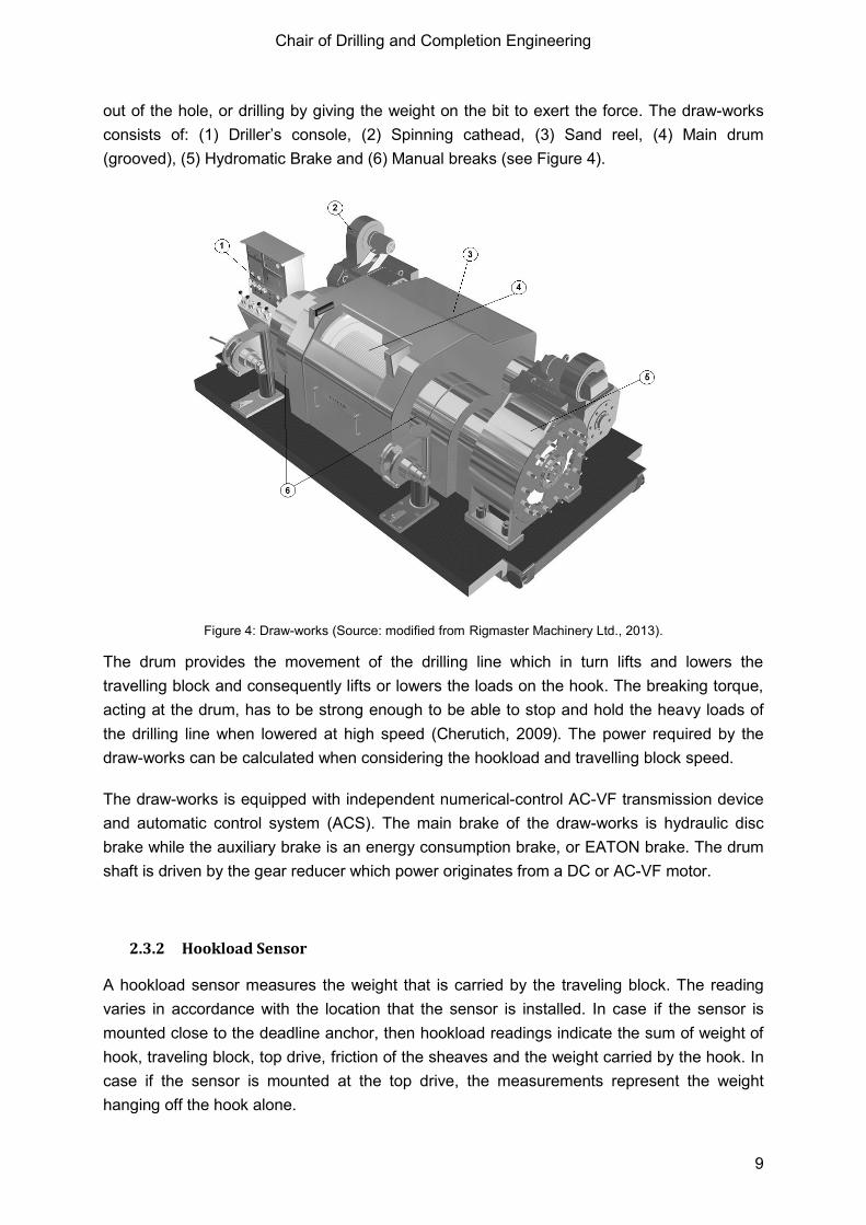
out of the hole, or drilling by giving the weight on the bit to exert the force. The draw-works
consists of: (1) Driller’s console, (2) Spinning cathead, (3) Sand reel, (4) Main drum
(grooved), (5) Hydromatic Brake and (6) Manual breaks (see Figure 4).
Figure 4: Draw-works (Source: modified from(Rigmaster Machinery Ltd., 2013).
The drum provides the movement of the drilling line which in turn lifts and lowers the
travelling block and consequently lifts or lowers the loads on the hook. The breaking torque,
acting at the drum, has to be strong enough to be able to stop and hold the heavy loads of
the drilling line when lowered at high speed (Cherutich, 2009). The power required by the
draw-works can be calculated when considering the hookload and travelling block speed.
The draw-works is equipped with independent numerical-control AC-VF transmission device
and automatic control system (ACS). The main brake of the draw-works is hydraulic disc
brake while the auxiliary brake is an energy consumption brake, or EATON brake. The drum
shaft is driven by the gear reducer which power originates from a DC or AC-VF motor.
2.3.2 Hookload Sensor
A hookload sensor measures the weight that is carried by the traveling block. The reading
varies in accordance with the location that the sensor is installed. In case if the sensor is
mounted close to the deadline anchor, then hookload readings indicate the sum of weight of
hook, traveling block, top drive, friction of the sheaves and the weight carried by the hook. In
case if the sensor is mounted at the top drive, the measurements represent the weight
hanging off the hook alone.

Chair of Drilling and Completion Engineering
10
2.3.3 Travelling Block Sensor
A travelling block sensor, also known as a block position sensor, measures the distance
between the travelling block and the rig floor. Usually this sensor can be mounted at the
draw-works and counts the revolutions of the draw-works drum per unit time. The number of
revolutions is multiplied by the circumference of the draw-works drum plus the layers of
drilling line on the drum to find the travelling block movement.
2.4 Circulating System
The principle components of the mud circulation system are: mud pumps, flow lines, drill
pipe, nozzles, mud mixing equipment, mud pits and tanks (mixing tank, suction tank, and
settling tank) as shown in Figure 5.
The flow path of the drilling fluid, that is called mud, can be described as from the mud pit to
suction line and to the pumps. At the pump the mud is pressured up and pumped through the
stand pipe, the rotary rose, via the swivel into the drill string. The mud circulates through the
drilling bit as it cuts through rock. The fluid lubricates the bit, removes rock cuttings, stabilizes
the wellbore wall, and controls the pressure in the wellbore. The mud then from the bottom of
the well rises up the annulus to the mud cleaning system that consists of shale shaker,
settlement tank, desander and desilter. After cleaning the mud, the circulation circle is closed
when the mud returns to the mud pit.
Figure 5: Circulation system (Source: Prassl, 2002).

Chair of Drilling and Completion Engineering
11
2.4.1 Mud Pumps
The mud pumps are large pumps used to move drilling fluid through the well bore when
performing drilling operation. The pump circulates the mud by pushing it down into the hole
through the drill string, and then moving it back up again, through the annulus. Mud pumps
are axial reciprocating piston pumps, meaning that they use oscillating pistons to displace
the fluid (see Figure 6).
Figure 6: Triplex mud pumps (Source:(NOV, 2014).
The mud pump is an axial piston pump that moves the fluid in only one direction. The power
end converts the rotation of the motor through the drive shaft to the reciprocating motion of
the axial pistons. In most cases a cross head crank gear is used for this.
Figure 7: Single acting piston schematic (Source: (GlobalSpec Inc., 2013).
There are two main parameters to measure the performance of a Mud Pump: Displacement
and Pressure. Displacement is measured as discharged liters per minute. In order to remove
all the cuttings from the hole and prevent settling and dropouts, a certain fluid velocity is
required depending on the size of the cuttings and the viscosity of the drilling fluid. The larger
the diameter of the drilling hole, the larger the necessity of displacement. The required
annular fluid velocity is generally in the range of 0.4 to 1.0 m/min.
To move the drilling fluid a pressure is required to overcome the frictional forces along the
drill pipe and the annulus of the hole. The deeper the well the greater the resulting pipeline
resistance, the higher the pressure required.
In the Mud Pump mechanism, the gearbox or hydraulic motor is equipped to adjust its
pressure and displacement to accommodate for the changing displacement requirements
during drilling. To this end, a flowmeter and a pressure gauge are installed in the Mud Pump.
Most modern mud pumps are triplex-style pumps, which have three cylinders. The triplex

Chair of Drilling and Completion Engineering
12
pumps are generally lighter and more compact than the older duplex pumps and their output
pressure pulsations are not as large. The overall efficiency of a triplex mud pump is the
product of the mechanical and the volumetric efficiency. The mechanical efficiency is often
assumed to be 90% and is related to the efficiency of the prime mover itself and the linkage
to the pump drive shaft. The volumetric efficiency of a mud pump with adequately charged
suction system can be as high as 100%. Therefore most manufactures rate their pumps with
a total efficiency of 90% (Prassl, 2002).
2.4.2 Flow Rate Sensor
Flow rate (In): one of the most common methods of measuring the flow through an axial
piston pump is to count the strokes over time and calculate the volume of each stroke.
Accuracy of this flow meter is within 0.2-0.3% of the reading value (Singh, 2003).
Flow rate (Out): there are different sensors in use for this measurement, and it is common
that the readings of flow rate out of these sensors vary from accurate to non-accurate results
depending on the technology used. One of the most common technologies is the use of a
flow paddle positioned in the flow line between the well and the shakers, which provide not
accurate results since the wear of the paddles generates an error. Once high accurate data
is necessary the technology used is the Coriolis type sensors. Coriolis sensors are classified
as multivariable, as they provide a measurement of mass and volume flow rate, density and
temperature. The mass flow rate accuracy is ±0.5% of rate at the best operating conditions.
The sensor consists of a manifold which splits the fluid flow into two, and directs it through
each of the two flow tubes and back out the outlet side of the manifold (Al-Morakhi, et al.,
2013).
2.4.3 Pump Pressure Sensor
Surface pressure sensors are usually located close to the pump and the reading is done by
the use of a diaphragm to isolate the mud from a gauges hydraulic fluid. For electrical
sensors, a transducer may have a diaphragm separating the mud from an electronic strain
gauge package, or the mud may act directly on the transducers steel bulkhead.
2.4.4 Mud Density Sensor
Density sensors do not always provide rapid and accurate measurements of drilling fluid
density. The density sensor is also used to monitor the addition of weighting material or fluid
to the mud system. Mud density is measured by two pressure sensors immersed at different
depths in the mud pit. Thus, mud density is calculated from the pressure differential and
depth between the sensors (Schlumberger, 2012).
Chair of Drilling and Completion Engineering
13
2.5 Power System
The power system of a drilling rig has to supply the following main components: rotary
system, hoisting system, and circulation system. In addition, auxiliaries like the blowout
preventer, boiler-feed water pumps, rig lighting system, among others have to be powered.
Since the largest power consumers on a drilling rig are the rotary, hoisting and the circulation
system, these components determine the total power requirements.
In the past, in ordinary drilling operations, the hoisting (lifting and lowering of the drill string,
casings, among others) and the circulation system were not operated at the same time.
Therefore the same engines were engaged to perform both functions. But in today’s drilling
operations, due to the increasing complexity of the wells to be drill, the hoisting and the
circulating system have to be operated at the same time (e.g. back reaming operations).
Therefore the drilling rig power system must be able to provide sufficient power for all the
equipment at the same time.
The power can be obtained mainly in two ways: (1) generated at the rig site using internal-
combustion diesel engines or gas turbines – depending of the availability of each fuel; or (2)
taken as electric power supply from existing power lines. As a guideline, the generated
power at the rig site is supplied with three/four engine/generator sets, each engine has a
power output between 1000 and 2000 [hp] (Prassl, 2002). The raw power is then transmitted
to the operating equipment via mechanical drives, DC or AC applying a variable frequency
drive (VFD). As mentioned before in Section 2, most of the newer rigs using the AC VFD
systems. The model developed in this work can only be utilized for these types of rig.
The rig power system’s performance is characterized by the output horsepower, torque and
fuel consumption for various engine speeds. The following section provides a more detailed
description of the diesel generator and the fuel consumption for the different engine speeds.
Section 2.5.2 describes the working principles, design characteristics, and equipment
efficiencies of the VFD system.
2.5.1 Diesel Generator
A diesel generator is the combination of two parts, a diesel engine and an electric generator,
to generate electrical energy. The first part, the diesel engine, works the same as any normal
internal combustion piston engine. It has an output shaft attached to the crank (the same as
any car engine) which is connected to the electric generator. The second part, the electric
generator, is a large alternator. The shaft of the alternator is driven by the diesel engine.
Thus, the diesel engine burns fuel (diesel) to rotate the generator shaft and produce
electrical energy.
Today, the majority of the new oil and gas drill rigs are AC electric rigs with VFD controls.
These rigs use multiple diesel-electric generator sets running in parallel to produce the two to

Chair of Drilling and Completion Engineering
14
four MW of power needed at the drill site, including the power needed for camp loads such
as lighting, heating and air conditioning for crew quarters.
Power is generated as AC and then directly connects with the VFD room. The VFD unit
allows precise control of the flow of power to any of the rig’s AC motor loads while the
generators running at a constant speed (load).
The number of generators needed by a rig varies with the depth of the drilling operation, but
today drillers have to go deeper vertically and sometimes just as far horizontally, and that
requires more power. Generator sets can easily be added to the AC powered rig to match
the power requirements, making this design the most flexible. The number of generator sets
running at the same time can be varied, depending on total load and fuel saving. This
configuration is also more reliable because a failure of one of the generator sets does not
necessarily cause a shutdown of drilling operations even though it may reduce the total
amount of power available. An additional advantage of paralleled generator sets is that
individual units can be taken offline for maintenance without greatly affecting the drilling
operation.
Fuel Consumption
Since drilling rig generator sets operate continuously, fuel consumption accounts for the
largest operational cost. Just a few percentage points of better fuel economy can add a
significant number of dollars to the bottom line at the completion of a well. Diesel engines
tend to be most fuel-efficient in proportion to their output when operated at 100 percent of
their rated load. Engines are typically rated in terms of their brake specific fuel consumption
(BSFC), which varies with the percentage of rated load. The BSFC rating allows comparing
the fuel economy of generator sets before the units are in the field. For 1,200-rpm generators
sets with a rating of about 1,100 kW, the BSFC should be less than 200 grams of fuel per
kWh generated. For maximum fuel economy it is recommended to always operate the
generator sets as near their nameplate rating as possible.
The fuel consumption of a generator changes as the elevation above mean sea level
changes. With the increase of the height there is power loss due to reduction in air mass flow
and poor combustion efficiency due to change in the resulting injection characteristics. The
power output of diesel engines falls at the rate of about one per cent for every 100 m altitude
(Sivasankaran & Jain, 1988).
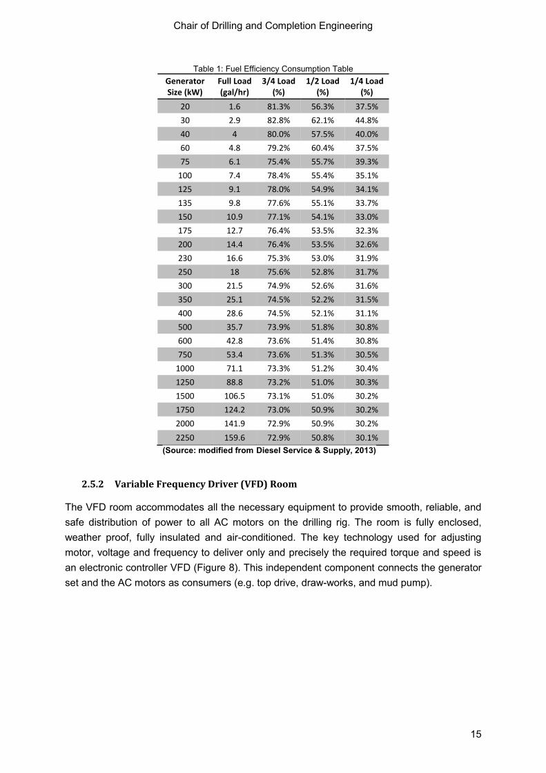
The table below approximates the fuel consumption of a diesel generator based on the size
of the generator and the load at which the generator is operating. Please, note that this table
is intended as an estimation of how much fuel a generator uses during operation and it is not
an exact representation due to various factors that can increase or decrease the amount of
fuel consumed.
Chair of Drilling and Completion Engineering
15
Table 1: Fuel Efficiency Consumption Table
Generator Size (kW)
Full Load (gal/hr)
3/4 Load (%)
1/2 Load (%)
1/4 Load (%)
20 1.6 81.3% 56.3% 37.5%
30 2.9 82.8% 62.1% 44.8%
40 4 80.0% 57.5% 40.0%
60 4.8 79.2% 60.4% 37.5%
75 6.1 75.4% 55.7% 39.3%
100 7.4 78.4% 55.4% 35.1%
125 9.1 78.0% 54.9% 34.1%
135 9.8 77.6% 55.1% 33.7%
150 10.9 77.1% 54.1% 33.0%
175 12.7 76.4% 53.5% 32.3%
200 14.4 76.4% 53.5% 32.6%
230 16.6 75.3% 53.0% 31.9%
250 18 75.6% 52.8% 31.7%
300 21.5 74.9% 52.6% 31.6%
350 25.1 74.5% 52.2% 31.5%
400 28.6 74.5% 52.1% 31.1%
500 35.7 73.9% 51.8% 30.8%
600 42.8 73.6% 51.4% 30.8%
750 53.4 73.6% 51.3% 30.5%
1000 71.1 73.3% 51.2% 30.4%
1250 88.8 73.2% 51.0% 30.3%
1500 106.5 73.1% 51.0% 30.2%
1750 124.2 73.0% 50.9% 30.2%
2000 141.9 72.9% 50.9% 30.2%
2250 159.6 72.9% 50.8% 30.1%
(Source: modified from(Diesel Service & Supply, 2013)
2.5.2 Variable Frequency Driver (VFD) Room
The VFD room accommodates all the necessary equipment to provide smooth, reliable, and
safe distribution of power to all AC motors on the drilling rig. The room is fully enclosed,
weather proof, fully insulated and air-conditioned. The key technology used for adjusting
motor, voltage and frequency to deliver only and precisely the required torque and speed is
an electronic controller VFD (Figure 8). This independent component connects the generator
set and the AC motors as consumers (e.g. top drive, draw-works, and mud pump).

Chair of Drilling and Completion Engineering
16
Figure 8: Schematic variable‐frequency drive (Wikipedia, 2013).
The VFD usual design is first converts AC input power to DC intermediate power using a
rectifier or converter bridge. The rectifier is usually a three-phase, full-wave-diode bridge.
The DC intermediate power is then converted to quasi-sinusoidal AC power using an inverter
switching circuit. The inverter circuit is probably the most important section of the VFD,
changing DC energy into three channels of AC energy that can be used by an AC motor.
These units provide an improved power factor, less harmonic distortion, and low sensitivity to
the incoming phase sequencing than older phase controlled converter VFD’s. The VFD is
mostly based on pulse width modulation. It has power demand in both standby and
subsequent variable operational modes, so additional losses of a VFD have to be over
compensated by reducing losses in partial load.
Many of the new motor technologies operate with variable speeds. This means that they
electronically adapt the speed rather than being based on a fixed speed design with 2, 4, 6 or
8 poles. Advanced adjustable speed controllers offer several advantages (Waide & Brunner,
2011):
They can eliminate the major source of partial‐load losses, such as mechanical
resistance elements (throttles, dampers, bypasses).
Adjustable speed and torque systems can be used for direct drive, eliminating
unnecessary components such as gears, transmissions and clutches, and reducing
cost and losses.
Maintenance costs can be lowered, since lower operating speeds result in longer life
for bearings and motors.
A soft starter for motor is no longer required.
Ability of a VFD to limit torque to a user-selected level can protect drive-equipment
that cannot tolerate excessive torque.
AC motor characteristics require the applied voltage to be proportionally adjusted whenever
the frequency is changed in order to deliver the rated torque. For example, if a motor is
designed to operate at 460 volts at 60 Hz, the applied voltage must be reduced to 230 volts
when the frequency is reduced to 30 Hz. Thus the ratio of volts per hertz must be regulated

Chair of Drilling and Completion Engineering
17
to a constant value (460/60 = 7.67 V/Hz in this case). For optimum performance, some
further voltage adjustment may be necessary especially at low speeds, but constant ratio of
volts per hertz is a general rule. This ratio can be changed in order to change the torque
delivered by the motor (Automation Consulting, LLC, 2011).
In addition to this simple volts-per-hertz control more advanced control methods such as
vector control and direct torque control (DTC) exist. These methods adjust the motor voltage
in such a way that the magnetic flux and mechanical torque of the motor can be precisely
controlled
VFDs consume energy within their control circuits (motor control, network connection,
input/output [I/O] logic controllers, etc.) and lose energy, particularly in the output switches.
The losses of these inverters are relatively low and their efficiency in partial load is typically
better than cage induction motors. VFDs also induce further losses in the motor due to
harmonic distortion and non-sinusoidal output-voltage waveform. The main influencing
factors on total losses are the switching frequency and the output current (which is basically
associated with output power and load). Waide & Brunner (2011) presents the variable
frequency drive efficiencies for different VFD nominal output power and motor loads (Figure
9).
Figure 9: VFD efficiency at full and partial load. (Source: Waide& Brunner, 2011)

Chair of Drilling and Completion Engineering
18
2.6 Other Rig Sensors
This section presents readings that can be calculated with the help of other sensors.
2.6.1 Hole Depth Readings
Hole Depth reading provides the depth of the hole drilled. It is a calculated channel based on
Bit Depth Readings (see next) and typically reflects the largest bit depth reached at any point
in time. This measurement usually requires manual resets and is prone to errors based on
that.
2.6.2 Bit Depth Readings
Bit Depth is typically a distance between a surface reference point (e.g. rotary kelly bushing)
and the bit location in the hole. These readings help the driller determine the location of the
drill bit in the wellbore. It is a calculated channel based on the Block Height readings and the
drill string pipe tally sheet.
2.6.3 Weight on Bit Readings
Weight on Bit (WOB) is calculated by subtracting the theoretical weight of drill string from
hookload measurements while the bit is on bottom. These readings help the driller to
estimate how much weight is applied on the drill bit. There is no WOB while tripping
operations, since the bit is not on the bottom of the hole. The measurement typically does not
consider friction in the form of drag. Thus for inclined or horizontal wells the WOB will reflect
a wrong number.

Chair of Drilling and Completion Engineering
19
3. Energy Consumption Mathematical Model
A quantitative description of a physical process always requires a mathematical formulation.
These mathematics aim at approximating the process in the best possible wayand refer to
the most important aspects. These mathematics are summarized by the term mathematical
model (Heinemann, 2005).
This chapter describes the mathematical model that was created to simulate the energy
consumption of a drilling rig. Any system properties, which are not included in the
mathematical model cannot be taken into consideration for further calculations.
Drilling rigs are equipped with several electricity consuming components. To calculate the
energy consumption of a drilling rig, it is necessary to calculate energy consumed by each
component. Thus, the model created in this thesis simulates each of these three main
components, which are: top drive, mud pumps and draw-works. The remaining part of the
energy consumed by all the other extra equipment on the rig is also included into the model
in a more simplified way.
For a coherent description of the developed model, this chapter is divided into three sections.
The first section defines all input data, which are necessary to run the model. The second
section explains necessary concepts (e.g. energy, power, efficiencies) and equations used to
develop the model. The third section deals with each component used for mathematical
model and describes them particularly. The third section is divided into five sub-sections. The
first four subsections present a detailed description of the steps taken to calculate the total
electrical power requirements for each of the four sub-models (i.e. top drive, mud pumps,
draw-works, and extra equipment). The last sub-section presents an integration of the four
sub-models into one final result of total energy required per unit of time.
3.1 Input Data
The process of mathematical model development aims to combine both, accuracy in the
results and least amount of data to run the model. The requirement of least data is essential
for many oil companies, which are limited in terms of gathering and sharing information with
the third parties. Thus, a complicated model that requires a lot of inputs to run is not in
demand based on the research and market investigation of the company supporting this
thesis.
As result of the research, the following information was chosen to be used as input to run the
model:
Drilling data channels (Date; Time; Block Height; Hookload; Top Drive RPM; Top
Drive Torque; Flow In Rate; Pressure Pump; Mud Weight);

Chair of Drilling and Completion Engineering
20
Specification of the rig equipment (mud pumps, draw-works, top drive, VFD room,
other equipment).
The flow chart below presents a simple visualization of the suggested model.
Dri
llin
g D
ata
Ch
ann
els
Energy Consumption Mathematical Model
Mud Pumps
Draw-works
Top DriveTop Drive
Extra Equipment
Total Electrical Rig Requirement
Rig Systems Specifications: -> Mud Pumps; -> Draw-works; -> Top Drive; ->Extra Equipment;
FlowIn/Pressure/MW
Hookload/PosBlock
RPM/TorqueRPM/Torque
Input Data
Figure 10: Energy consumption model flow chart.
3.1.1 Drilling Data Channels
The drilling data channels reflect the information recorded by rig sensors. This information is
gathered in real time and transmitted via WITSML to a data base, where it is stored. Drilling
data can have different sampling frequencies and is specified by a mud logging company
collecting the data set. Table 2 presents the name, dimension, and units from the drilling data
channel used in this thesis.
Table 2: Minimum set of data channels.
Channel Dimension Unit
Block Height length m
Flow In Rate volumeover time m3/h
Hookload weight kg
Top Drive RPM 1 over time rpm
Top Drive Torque forcebylength N.m
Pressure Pump pressure Pa
MudWeight weightovervolume kg/m3
Table 3 depicts the drilling data channels that are used as input information for the model
and also presents one minute of real drilling data. Further, this drilling data example is used
as a base for several calculations and examples during the thesis. These data are collected
at the sampling frequency of 0.2 Hz (sampling period of 5seconds).

Chair of Drilling and Completion Engineering
21
Table 3: Drilling Data used in the model with 0.2 Hz sampling frequency.
Date Time Block Height
[m]
Flow In Rate
[m3/h]
Hookload [kg]
Top Drive RPM [rpm]
Top Drive Torque [N.m]
Pressure Pump
[mH2O]
MudWeight [kg/m3]
14.09.2013 06:00:00 35.5 190.1 65667 68.7 2454.2 1459.1 1521.8
14.09.2013 06:00:05 35.4 206.4 65077 71.4 2118.0 1635.0 1521.8
14.09.2013 06:00:10 35.1 206.4 64442 71.4 2259.0 1639.1 1521.8
14.09.2013 06:00:15 34.8 206.4 62265 71.1 4006.8 1652.3 1521.8
14.09.2013 06:00:20 34.6 206.4 58500 71.0 6142.4 1725.3 1521.8
14.09.2013 06:00:25 34.4 206.4 58817 71.0 6378.3 1735.7 1521.8
14.09.2013 06:00:30 34.2 206.4 58817 71.3 5844.1 1737.3 1521.8
14.09.2013 06:00:35 34.0 206.4 58863 71.4 5732.9 1739.0 1521.8
14.09.2013 06:00:40 33.8 206.4 58681 71.4 5768.1 1737.1 1521.8
14.09.2013 06:00:45 33.6 206.4 58409 71.4 5917.3 1793.2 1521.8
14.09.2013 06:00:50 33.3 206.4 56640 71.1 7578.3 1855.7 1521.8
14.09.2013 06:00:55 33.0 206.4 53783 71.2 8470.5 1896.9 1521.8
14.09.2013 06:01:00 32.7 206.4 52830 71.4 8886.8 1929.8 1521.8
The frequency of 0.2 Hz was chosen as input in the mathematical model because of two
main reasons. The first is that sampling frequency smaller than 0.2 Hz does not represent
the dynamic behavior of operations of the rig correctly. Thus the results collected with this
frequency would be wrong. The second reason is that the drilling data usually is provided via
WITSML protocol, which has a sampling frequency of 0.1 - 0.2 Hz.
There are two ways to obtain necessary drilling data in order to run the Energy Consumption
Mathematical Model. The first option is to access real drilling data. For that it is necessary to
have authorization. Once the authorizations are granted, the data base can be accessed via
web and necessary drilling data to run the model can be downloaded. The second option is
to use the Drilling Data Simulator to generate the drilling data based on the pre-defined well
plan.
3.1.1.1 Drilling Data Quality Control
The drilling data channels may contain problems from different sources such as: physically
damaged sensors, incorrectly calculated data channel, wrong sensor calibration, among
others. Thus, a quality control of the data should be performed before the data is used. The
following list represents the quality control health checks that can be performed to evaluate
data quality: validity, accuracy, consistency, integrity, timeliness, completeness and
continuity (Arnaout, Zoellner, Johnstone, & Thonhauser, 2013).
Quality management analysis of the data channels was developed in order to assure the
quality of the input data used in the model. The two main quality management steps, which

Chair of Drilling and Completion Engineering
22
are used in this thesis, are data standardization and data quality control as proposed in
(Mathis & Thonhauser, 2007).
Data Standardization
Data standardization is the first and the most crucial step in quality management analysis.
Different problems need to be analyzed to assure data quality. The problems analyzed in this
thesis are:
Unit definition – to use the data, the units of the measurements needs to be defined
to ensure the correct transformation to the units used by the model;
Null values–a null value is a value used to signify that a specific value does not have
a valid measurement. The value used in practice is -999.25. The null value needs to
be standardized to allow the correct treatment of this data before it is used by the
model;
Time stamping and time zones – the use of a standardized data and time.
Data Quality Control
Data quality control from this thesis consists of the following steps:
Range check – simple analysis if the range of the channels fits the model. This is
based on the frequency that the data is sampled. In this thesis a period of 24 hours is
used;
Null values filling – all the null values in the data are replaced for the value of zero.
Thus, the null values do not influence the final results;
Outlier removal – this analysis removes unrealistic values from the data based on cut-
off created with the use of the rig system specifications.
All the steps above are performed automatically to facilitate the use of the model.
Rig Systems Specifications
The specification of the rig equipment is obtained from the manufactures of the equipment.
The main necessary information includes equipment power rating and efficiencies (i.e. motor
efficiency for 50%, 75%, and 100% of loading and overall efficiency). Also, it is necessary to
have an estimated overall value for the power consumption of all other equipment (i.e.
excluding top drive, mud pumps and draw-works).This information is used as input for the
mathematical model described in the following sections of the thesis. The table below shows
an example of necessary information for the equipment specification.

Chair of Drilling and Completion Engineering
23
Table 4: Top drive, mud pumps and draw-works necessary specifications.
Top Drive Mud Pumps Draw-works
Power Rating [kW]: 500 Power Rating [kW]: 500 Power Rating [kW]: 500
Top Drive Weight [kg]: 15000 Overall Eff. [%]: 85% Overall Eff. [%]: 85%
Overall Eff. [%]: 85% Overall Eff. [%]: 85%
Load Efficiency Load Efficiency Load Efficiency
50% 93.50% 50% 94.90% 50% 94.50%
75% 94.70% 75% 95.20% 75% 94.10%
100% 95.10% 100% 94.80% 100% 93.20%
3.2 General Energy Consumption Concepts
The total energy required by the equipment for an AC Electrical Drilling Rig is the electrical
energy provided by the AC generator. All the equipment use AC current to power their
motors to perform a certain work. The total energy required can be calculated by:
[ ] Eq. 1
where:
- Energy [J];
- Electrical Power [W];
- Time [s].
The equation above defines that the consumed energy is the product of electrical power
required for the equipment to perform a certain work, multiplied by the time period for which
this power was required. The Joule, symbol J, is a derived unit of energy, work or amount of
heat in the International System of Units.
The electrical power required by the equipment to perform some work can be calculated
from:
[ ] Eq. 2
where:
- Mechanical or Hydraulic Power [W];
- Overall efficiency [%];
- Motor efficiency [%];
- VFD efficiency [%].
Chair of Drilling and Completion Engineering
24
A different way to present the same equation is:
∑ ∑ ∑ [ ] Eq. 3
where:
∑ - Overall Losses [W];
∑ - Motor Losses [W];
∑ - VFD Losses [W].
The standard metric unit of power is the Watt (W). As it is implied by Eq. 1, a unit of power is
equivalent to a unit of energy divided by a unit of time. Thus, a Watt is equivalent to a
Joule/second.
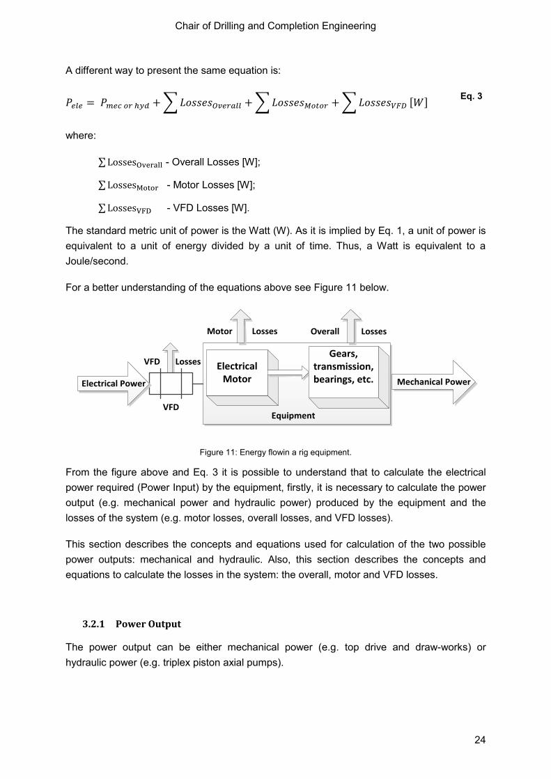
For a better understanding of the equations above see Figure 11 below.
Mechanical Power
Motor Losses
Electrical Motor
Overall Losses
Gears, transmission, bearings, etc.
Equipment
VFD Losses
VFD
Electrical Power
Figure 11: Energy flowin a rig equipment.
From the figure above and Eq. 3 it is possible to understand that to calculate the electrical
power required (Power Input) by the equipment, firstly, it is necessary to calculate the power
output (e.g. mechanical power and hydraulic power) produced by the equipment and the
losses of the system (e.g. motor losses, overall losses, and VFD losses).
This section describes the concepts and equations used for calculation of the two possible
power outputs: mechanical and hydraulic. Also, this section describes the concepts and
equations to calculate the losses in the system: the overall, motor and VFD losses.
3.2.1 Power Output
The power output can be either mechanical power (e.g. top drive and draw-works) or
hydraulic power (e.g. triplex piston axial pumps).

Chair of Drilling and Completion Engineering
25
3.2.1.1 Mechanical Power
Mechanical power is the product of forces and movements. In particular, power is the product
of a force on an object and the object's velocity, or the product of a torque on a shaft and the
shaft's angular velocity.
By definition,
[ ]
Eq. 4
where:
- Force [N];
- Distance [m].
Deriving the previous equation results in:
[ ] Eq. 5
where:
- Torque [N.m];
- Rotation [rpm].
As an example, from Eq. 5, it is possible to conclude that with the drilling data channels
torque and RPM from a top drive (see Table 3) it is possible to calculate the mechanical
power produced by this equipment.
3.2.1.2 Hydraulic Power
Hydraulic Power is characterized by the main variables, pressure and flow, whose product
results in power. Pressure is force per unit area and flow Q is volume per time. For hydraulic
calculations, the fluid is generally assumed incompressible.
By definition, the hydraulic power is calculated as:
[ ]
Eq. 6
where:
- Pressure [Pa];
- Flow In [m3/h];
- Gravity [m/s2];

Chair of Drilling and Completion Engineering
26
- Fluid density [kg/m3].
As an example, from Eq. 6, it is possible to conclude that drilling data channels pump
pressure, flow-in rate and mud weight from the mud pump (see Table 3) allow to calculate
the hydraulic power performed by this equipment.
.
3.2.2 System Losses and Efficiency
The efficiency can be defined as the ratio of the output power to the input power, and is
usually expressed as a percentage (η is the Greek letter neta). The output power of
equipment is always less than the input power because some of the energy supplied is lost
(see Figure 11).The losses in machines are forms of output energy which is not used and,
therefore, not desired. An electric motor converts electrical energy into mechanical energy,
but also produces heat which is not desired. This heat is a loss. It means that the heat is
generated, but is not used. Losses occur in all types of machines and take many forms other
than heat such as sound, vibration and internal resistance. The effect of losses is the
reduction of efficiency of a machine (Australian, 2008).
The general formula of efficiency is presented below:
Eq. 7
where:
- Efficiency [%];
- Output power [W];
- Output power [W].
Another way to represent efficiency of a system is to estimate the total losses of the system.
∑ [ ] Eq. 8
where:
∑ - Losses [W].
Combining both equations it is possible to derive the following equation:
∑ (
) [ ]
Eq. 9
In Eq. 9 the losses of equipment are related to the efficiency of the system and output power.
In this thesis the model simplifies all the losses into:

Chair of Drilling and Completion Engineering
27
Overall losses – fixed value related to the mechanical system to which the motor is
coupled;
Motor losses - varies according with the load of the motor;
VFD losses – varies according with the electrical power required by the motor.
3.2.2.1 Overall Losses
As in any equipment the overall efficiency varies according with the load applied. As stated in
(Azar & Samuel, 2007) and manufacture manuals (e.g. Aker Wirth and Bentec), a fixed value
of efficiency is adopted to represent all energy losses (e.i. transmission, gear, bearing,
friction, hydraulic, volumetric, among others).In electric motor-driven systems, additional
energy losses occur in the motor itself, the section below explains these losses.
This thesis describes models of three types of equipment that are the main energy
consumers in a drilling rig. Moreover, the model considers the overall losses of the systems
that are related to each equipment. The overall losses are described in the respective sub-
sections of the following Section 3.3, where a mathematical model for each equipment is
presented.
3.2.2.2 Motor Efficiency and Losses
A motor’s function is to convert electrical energy into mechanical energy to perform useful
work. The only way to improve motor efficiency is to reduce motor losses. Motor energy
losses can be segregated into five major areas, each of which is influenced by design and
construction decisions. Motor losses may be categorized as those which are fixed, occurring
whenever the motor is energized, and remaining constant for a given voltage and speed, and
those which are variable and increase with the motor load (McCoy, Litman, & Douglass,
1993). These losses are described below and after summarized in the Table 5.
1. Core loss represents energy required to magnetize the core material (hysteresis)
and includes losses due to creation of eddy currents that flow in the core. Core
losses are decreased through the use of improved permeability electromagnetic
(silicon) steel and by lengthening the core to reduce magnetic flux densities. Eddy
current losses are decreased by using thinner steel laminations (Saidur, 2009).
2. Friction losses occur due to bearing friction and air resistance. Improved bearing
selection, air-flow and fan design are employed to reduce these losses. In an
energy-efficient motor, loss minimization results in reduced cooling requirements
so a smaller fan can be used. Both core losses and friction losses are
independent of motor load (Saidur, 2009).
3. Stator losses appear as heating due to current flow (I) through the resistance (R)
of the stator winding. This is commonly referred to as an I2R loss. I2R losses can
be decreased by modifying the stator slot design or by decreasing insulation
thickness to increase the volume of wire in the stator (Saidur, 2009).

Chair of Drilling and Completion Engineering
28
4. Rotor losses appear as I2R heating in the rotor winding. Rotor losses can be
reduced by increasing the size of the conductive bars and end rings to produce a
lower resistance or by reducing the electrical current (Saidur, 2009).
5. Stray load losses are the result of leakage fluxes induced by load currents. Both
stray load losses and stator and rotor I2R losses increase with motor load (Saidur,
2009).
Table 5: Motor loss categories
As described above the variation of motor losses occurs due to motor loading. These losses
are the same for each of the motors in a drilling rig. Thus, the description to calculate the
motor losses is only presented in this section, but the calculation is performed for each of the
equipment modeled in this thesis.
To calculate the motor losses firstly it is necessary to obtain from the manufacturer of the
motor the efficiencies for the loads 50%, 75% and 100%. By using Eq. 9 with the loads and
efficiencies of the equipment it is possible to calculate the losses for the loads 50%, 75% and
100% respectively (see Figure 12).
Figure 12: Variation in losses due to motor loading (Source: McCoy, Litman, & Douglass, 1993).

Chair of Drilling and Completion Engineering
29
The losses of an engine are composed of two parts. One part is proportional to the square of
the voltage (in our case considered constant) and another is proportional to the square of the
current. The current is proportional to the load. Thus the losses are composed of a fixed
component and a component proportional to the square of the load. A graph is created using
the values of the square of the load versus the losses (see Figure 13). A regression line can
be drawn to connect the points. The resulting straight line approximation (ax + b) gives the
fixed component of the losses (b) and the dependence of the square of the load (a). Thus the
equation representing this regression line can describe the motor losses for any load on the
motor. This procedure is adopted for the three modeled equipment described in the thesis.
Figure 13 shows a graphic of motor losses.
Figure 13: Motor losses by the square of the load of a top drive with the regression line.
3.2.2.3 VFD Losses
The VFD Losses calculate the energy losses of the VFD room for each equipment element.
As described in Section 2.5.2, the VFD room has power demand in both standby and
subsequent variable operational modes, so consequently losses vary according to the load
value (Burt, Piao, Gaudi, Busch, & Taufik, 2006).
The procedure of VFD losses calculation is complicated because the manufacturer does not
provide all necessary specification of the equipment for this calculation. Thus, to resolve this
issue, a general equation is created to calculate the efficiency of VFD based on studies
presented by Waide & Brunner (2011) and Burt et al. (2006).
[
]
Eq. 10
The Eq. 10 created in this thesis represents the efficiency of a variable speed drive varying
with the load. Such equation provides representative values of efficiencies for the equipment
modeled in this thesis. Figure below is a graphical representation of Eq. 10.
Total Losses = a x [Load]^2 + b
00
10
20
30
40
50
60
70
0% 20% 40% 60% 80% 100% 120%
Tota
l Lo
sse
s [k
W]
Load^2

Chair of Drilling and Completion Engineering
30
Figure 14: Graphic representation of the load vs. efficiency for the VFD.
Once the efficiency of the VFD is calculated for the corresponding load using Eq. 10, the
power losses of the VFD room can be calculated for the top drive, mud pumps, or draw-
works.
∑ [ ] Eq. 11
where:
- Equipment power [W].
3.3 Energy Consumption Models Description
The energy consumption model created in this thesis is divided into sub-models. There are in
total four sub-models and each of them represents a different system in the drilling rig.
The sub-models that represent the three main consumers in the rig (i.e. top drive, mud
pumps, draw-works) have the same procedure to calculate required electrical power. The
concepts and the equations necessary to understand and calculate the electrical power are
presented in Section 3.2. The procedures used in these three sub-models are:
1. Calculate the power output from the drilling data (i.e. mechanical power or
hydraulic power);
2. Calculate the overall losses with the power output and overall efficiency from the
rig manufacture using Eq. 9;
3. Calculate the load on the electrical motor. This can be accomplished by summing
the power output and overall losses and dividing it by equipment power rating:
90%91%92%93%94%95%96%97%98%99%
100%
0% 20% 40% 60% 80% 100% 120%
Effi
cie
ncy
Load
VFD - Efficiency vs. Load

Chair of Drilling and Completion Engineering
31
∑
[ ] Eq. 12
where:
- Load [%]
4. Calculate the motor losses with the help of the regression equation created for
each equipment using the procedure described in Section 3.2.2.2;
5. Calculate the VFD efficiency using Eq. 10;
6. Calculate VFD losses based on the VFD efficiency and the electrical power
required by the motor (Eq. 11);
7. Calculate the total electrical power of the equipment as the sum of power output,
overall losses, motor losses and VFD losses (Eq. 3).
For the last sub-model (the Other Equipment) a different methodology is used. This
methodology is presented in the respective section of the sub-model.
3.3.1 Top Drive Energy Consumption Model
As presented in Section 2.1, the top drive has the same working principle as a motor, where
the motor transforms electrical energy into mechanical. To be able to calculate the electrical
energy consumption of the top drive it is necessary to calculate the mechanical power at the
shaft, overall losses, motor losses, and VFD losses (see Figure 15).
Mechanical Power
Motor Losses
Electrical Motor
Overall Losses
Gears, transmission, bearings, etc.
Dri
ll St
rin
gD
rill
Stri
ng
Torque RPM
Top DriveVFD
Electrical Power
VFD Losses
Figure 15: Energy flow in a top drive.
First, from the drilling data channels of torque and RPM it is possible to calculate the
mechanical power (Eq. 5). With the calculated mechanical power and overall efficiency
(provided by the rig manufacture) it is possible to calculate the overall losses using Eq. 9.The
second step is to calculate the motor losses. So, based on the procedures described in
Section 3.2.2.2 with the motor efficiencies for 50%, 75%, and 100% it is possible to calculate
the motor losses.
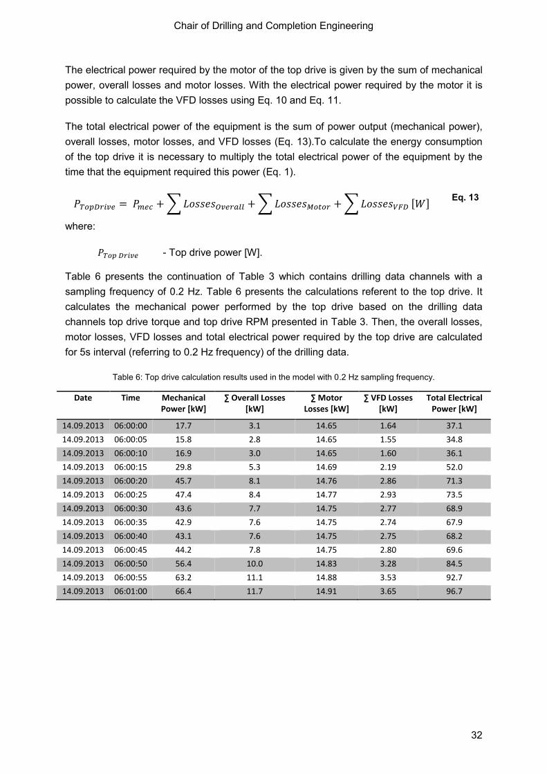
Chair of Drilling and Completion Engineering
32
The electrical power required by the motor of the top drive is given by the sum of mechanical
power, overall losses and motor losses. With the electrical power required by the motor it is
possible to calculate the VFD losses using Eq. 10 and Eq. 11.
The total electrical power of the equipment is the sum of power output (mechanical power),
overall losses, motor losses, and VFD losses (Eq. 13).To calculate the energy consumption
of the top drive it is necessary to multiply the total electrical power of the equipment by the
time that the equipment required this power (Eq. 1).
∑ ∑ ∑ [ ] Eq. 13
where:
- Top drive power [W].
Table 6 presents the continuation of Table 3 which contains drilling data channels with a
sampling frequency of 0.2 Hz. Table 6 presents the calculations referent to the top drive. It
calculates the mechanical power performed by the top drive based on the drilling data
channels top drive torque and top drive RPM presented in Table 3. Then, the overall losses,
motor losses, VFD losses and total electrical power required by the top drive are calculated
for 5s interval (referring to 0.2 Hz frequency) of the drilling data.
Table 6: Top drive calculation results used in the model with 0.2 Hz sampling frequency.
Date Time Mechanical Power [kW]
∑ Overall Losses [kW]
∑ Motor Losses [kW]
∑ VFD Losses [kW]
Total Electrical Power [kW]
14.09.2013 06:00:00 17.7 3.1 14.65 1.64 37.1
14.09.2013 06:00:05 15.8 2.8 14.65 1.55 34.8
14.09.2013 06:00:10 16.9 3.0 14.65 1.60 36.1
14.09.2013 06:00:15 29.8 5.3 14.69 2.19 52.0
14.09.2013 06:00:20 45.7 8.1 14.76 2.86 71.3
14.09.2013 06:00:25 47.4 8.4 14.77 2.93 73.5
14.09.2013 06:00:30 43.6 7.7 14.75 2.77 68.9
14.09.2013 06:00:35 42.9 7.6 14.75 2.74 67.9
14.09.2013 06:00:40 43.1 7.6 14.75 2.75 68.2
14.09.2013 06:00:45 44.2 7.8 14.75 2.80 69.6
14.09.2013 06:00:50 56.4 10.0 14.83 3.28 84.5
14.09.2013 06:00:55 63.2 11.1 14.88 3.53 92.7
14.09.2013 06:01:00 66.4 11.7 14.91 3.65 96.7

Chair of Drilling and Completion Engineering
33
3.3.1.1 Top Drive Overall Efficiency
The adopted top drive overall efficiency is a fixed value that represents the efficiency for the
rotary system (described in Section 2.2). This value estimation is based on the specification
of the equipment that considers all energy losses (e.g. transmission, gear, bearing, friction)
occurring in the rotary system.
Based on technical information for top drives from the company Aker Wirth it is possible to
estimate the top drive overall efficiency in the range of 80-90%. If it is not possible to obtain
this information from the top drive manufacturer, values can be assumed in the proposed
range.
3.3.2 Mud Pumps Energy Consumption Model
As mentioned in Section 2.4.1, the mud pumps are the triplex-single acting pumps. An
electrical motor provides mechanical energy for the axial-pistons to pump the drilling fluid.
The pump transforms electrical energy into hydraulic energy (Figure 16).
Hydraulic Power
Motor Losses Overall LossesFlow In Pressure
Mud Pump
Volumetric, Mechanic, Hydraulic Efficiency
Dri
ll St
ring
Dri
ll St
ring
Electrical Motor
VFD
Electrical Power
VFD Losses
Figure 16: Energy flow in a mud pump.
To calculate the electrical energy consumption of the mud pump it is necessary to calculate
the hydraulic power, overall losses, motor losses and VFD losses.
At first, from the drilling data channels of flow in, pressure and mud weight, it is possible to
calculate the hydraulic power (Eq.Eq. 6). With the calculated hydraulic power and overall
efficiency provided by the rig manufacture, it is possible to calculate the overall losses using
Eq. 9.The next step is to calculate the motor losses. So, based on the procedures described
in Section 3.2.2.2 with the motor efficiencies for 50%, 75% and 100% it is possible to
calculate the motor losses.
The electrical power required by the motor of the mud pump is given by the sum of hydraulic
power, overall losses and motor losses. With the known required electrical power it is
possible to calculate the VFD losses using Eq. 10 and Eq. 11.
The total electrical power of the equipment is the sum of power output (hydraulic power),
overall losses, motor losses and VFD losses (Eq. 3). To calculate the energy consumption of

Chair of Drilling and Completion Engineering
34
the mud pump, it is necessary to multiply the total electrical power of the equipment by the
time that the equipment required this power (Eq. 1).
∑ ∑ ∑ [ ] Eq. 14
where:
- Mud Pumps power [W]
Table 7 is the continuation of Table 3 which contains drilling data channels with a sampling
frequency of 0.2 Hz. Table 7 presents the calculations referent to the mud pumps. It
calculates the hydraulic power performed by the mud pumps based on the drilling data
channels Flow-In Rate, Pump Pressure, and Mud Weight presented in Table 3. Then, the
overall losses, motor losses, VFD losses and total electrical power required by the mud
pumps are calculated for the 5s interval (corresponding to 0.2 Hz frequency) of the drilling
data.
Table 7: Mud pump calculation results used in the model with 0.2 Hz sampling frequency.
Date Time Hydraulic Power [kW]
∑ Overall Losses [kW]
∑ Motor Losses [kW]
∑ VFD Losses [kW]
Total Electrical Power [kW]
14.09.2013 06:00:00 1150.1 171.9 64.34 38.16 1424.5
14.09.2013 06:00:05 1399.7 209.1 76.62 42.24 1727.7
14.09.2013 06:00:10 1403.2 209.7 76.81 42.29 1732.0
14.09.2013 06:00:15 1414.4 211.4 77.42 42.46 1745.7
14.09.2013 06:00:20 1476.9 220.7 80.91 43.32 1821.8
14.09.2013 06:00:25 1485.9 222.0 81.43 43.44 1832.8
14.09.2013 06:00:30 1487.2 222.2 81.50 43.46 1834.4
14.09.2013 06:00:35 1488.7 222.4 81.59 43.48 1836.2
14.09.2013 06:00:40 1487.1 222.2 81.49 43.46 1834.2
14.09.2013 06:00:45 1535.1 229.4 84.30 44.08 1892.8
14.09.2013 06:00:50 1588.6 237.4 87.52 44.74 1958.2
14.09.2013 06:00:55 1623.9 242.6 89.71 45.15 2001.4
14.09.2013 06:01:00 1652.0 246.9 91.49 45.47 2035.8
3.3.2.1 Mud Pump Overall Efficiency
The mud pump overall efficiency is a value that represents the efficiency for the circulating
system (described in Section 2.4). It is a variable that describes all energy losses in a
hydraulic system (e.g. hydraulic, mechanical, volumetric, friction), and its estimation is based
on the specification of the equipment (Rajput, 1998).
Overall pump efficiency is a ratio of power actually gained by the fluid to the shaft power
supplied. Overall efficiency is determined by multiplying hydraulic efficiency by mechanical
efficiency by volumetric efficiency by friction efficiency.
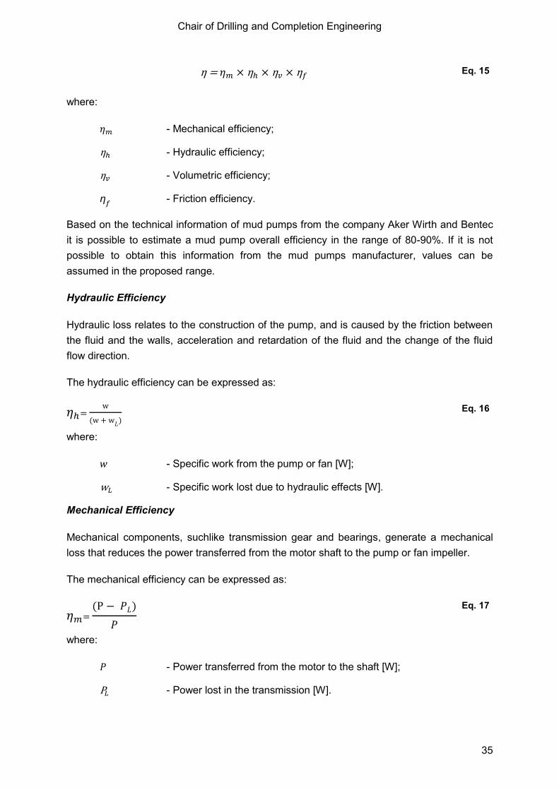
Chair of Drilling and Completion Engineering
35
Eq. 15
where:
- Mechanical efficiency;
- Hydraulic efficiency;
- Volumetric efficiency;
- Friction efficiency.
Based on the technical information of mud pumps from the company Aker Wirth and Bentec
it is possible to estimate a mud pump overall efficiency in the range of 80-90%. If it is not
possible to obtain this information from the mud pumps manufacturer, values can be
assumed in the proposed range.
Hydraulic Efficiency
Hydraulic loss relates to the construction of the pump, and is caused by the friction between
the fluid and the walls, acceleration and retardation of the fluid and the change of the fluid
flow direction.
The hydraulic efficiency can be expressed as:
Eq. 16
where:
- Specific work from the pump or fan [W];
- Specific work lost due to hydraulic effects [W].
Mechanical Efficiency
Mechanical components, suchlike transmission gear and bearings, generate a mechanical
loss that reduces the power transferred from the motor shaft to the pump or fan impeller.
The mechanical efficiency can be expressed as:
Eq. 17
where:
- Power transferred from the motor to the shaft [W];
- Power lost in the transmission [W].

Chair of Drilling and Completion Engineering
36
Volumetric Efficiency
Due to leakage of fluid between the back surface of the impeller hub plate and the casing, or
through other pump components, a volumetric loss reducing the pump efficiency can occur.
The volumetric efficiency can be expressed as:
Eq. 18
where:
- Volume flow out of the pump or fan [W];
- Leakage volume flow [W].
Friction Efficiency
Frictional efficiency corresponds to the pressure loss created by the fluid flowing through the
flow path. It is a function of fluid properties influenced by pressure and temperature (density,
viscosity, gel-strength), flow rate and the geometry of characteristic of flow path (hole
size/drill string size). Frictional pressure loss affects the pump pressure because higher
frictional pressure losses causes a higher pump pressure which is required to maintain the
desired pump rate (DrillingFormula, 2010).
3.3.3 Draw-works Energy Consumption Model
To calculate the energy consumption for the draw-works is a complicated task. As described
in Section 2.3, the draw-works has the same working principle as a motor, where the motor
transforms electrical energy into mechanical.
Motor Losses
Electrical Motor
Overall Losses
Dri
ll St
rin
gD
rill
Stri
ng
Block Height … … ….Hook load
Draw-works
Mechanical Power
Sheaves, gears, friction, crown/ traveling block
etc.
VFD
Electrical Power
VFD Losses
Figure 17: Energy flow in a draw-works.
The problem is that the drilling data channels do not provide the RPM and torque realized by
the draw-works. Thus, the mechanical power produced by the draw-works cannot be directly

Chair of Drilling and Completion Engineering
37
calculated. Further, studying the working principle of the hoisting system it is possible to
conclude that the energy consumption for trip-in and trip-out operations should be calculated
in different ways. For these reasons two different approaches are taken to calculate the
energy consumption by the draw-works. One of them simulates trip-in operations and the
other simulates trip-out operations. Both of them are explained in the following sections.
To understand if the rig is performing either tripping-in or tripping-out operations a simple
analysis of the Block Height can be performed. If Eq. 19 has a positive result, it means that
the rig is performing tripping-in operation, since the height of the block at is lower than
at (the drilling string is been lowered). And if Eq. 19 have a negative result, it means that
the rig is performing trip out operation, since the height of the block at is higher than
at (the drilling string is been lifted).
[ ] Eq. 19
where:
- Block height [m];
Based on this analysis, the following two energy consumption models are considered in
order to calculate the energy consumed by the draw-works.
3.3.3.1 Tripping-In Energy Consumption Model
The model developed for the energy consumption for tripping-in operations is based on the
principles that the draw-works use only breaks when lowering the drill string. Thus only a
fixed amount of power is required to activate the brakes (and not all the draw-works power is
necessary).
Eq. 20shows that the break power is constant. The value to be used as input can be found in
the specification of the draw-works.
[ ] Eq. 20
where:
- Break power [W].
3.3.3.2 Tripping-Out Energy Consumption Model
The model developed for the energy consumption in tripping-out operations is based on the
working principles of the hoisting system. After a careful analysis it is concluded that the
power required by the draw-works can be calculated using the hookload and travelling block
speed. In this section, the concept and mathematics used for these calculations are
described.
Chair of Drilling and Completion Engineering
38
Using the drilling data it is possible to calculate the mechanical power performed by the
draw-works from the Block Height and the Hookload channels. The idea is to calculate the
torque and the RPM performed by the draw-works drum based on these channels.
From the channel Block Height that describes the movement of the traveling block with
respect to the rig floor it is possible to convert the difference of the block height readings into
RPM of the draw-works. To achieve that, firstly, it is necessary to calculate the linear velocity
of the fast line (see Eq. 21).
|
| [
]
Eq. 21
where:
- Fast line linear velocity [m/s];
- Time difference [s];
- Number of sheaves .
Secondly, with the linear velocity and the drum radius of the draw-works it is possible to
calculate the angular velocity of the drum.
[ ] Eq. 22
where:
- Angular velocity [rpm];
- Drum radius [m].
From the channel Hookload that describes the weight carried by the hook and, consequently,
by the draw-works and the drum radius, it is possible to calculate the torque.
[ ]
Eq. 23
where:
- Hookload [kg].
From the calculated data of Torque (Eq. 23) and RPM (Eq. 22)it is possible to calculate the
mechanical power (Eq. 5). Thus, the mechanical power for the draw-works is calculated with
the combination of the Eq. 21, Eq. 22, and Eq. 23. The resultant equation from the
combination of those equations is presented below:
|
| [ ]. Eq. 24

Chair of Drilling and Completion Engineering
39
Analysis of the equation above leads to the conclusion that the information of number of
sheaves in the crown block/traveling block and the radius of the drum is not necessary for
the calculation of the mechanical power of the draw-works. This is explained by the fact that
the weight of the hookload applied at the draw-work is divided by the number of sheaves;
and, the same time, the draw-works speed is directly proportional to the amount of sheaves.
Thus, both parameters cancel each other out. It makes the mathematical model simpler
since fewer inputs are required.
With the calculated mechanical power and overall efficiency provided by the rig manufacture
it is possible to calculate the overall losses using Eq. 9.The next step is to calculate the
motor losses. So, based on the procedures described in Section 3.2.2.2 with the motor
efficiencies for 50%, 75%, and 100% it is possible to calculate the motor losses.
The electrical power required by the motor of the draw-works is given by the sum of
mechanical power, overall losses, and motor losses. With the required electrical power it is
possible to calculate the VFD losses using Eq. 10 and Eq. 11.
The total electrical power of the equipment is the sum of power output, overall losses, motor
losses and VFD losses (Eq. 25). To calculate the energy consumption of the draw-works, it
is necessary to multiply the total electrical power of the equipment by the time that the
equipment required this power (Eq. 1).
∑ ∑ ∑ [ ] Eq. 25
where:
- Draw-works power [W].
Table 8: Draw-works calculation results used in the model with 0.2 Hz sampling frequency.
Date Time Linear Vel.
[m/s]
Angular Velocity [RPM]
Torque [N.m]
Mech. Power [kW]
∑ Overall Losses [kW]
∑ Motor Losses [kW]
∑ VFD Losses [kW]
Total Elec.
Power [kW]
14.09.2013 06:00:00 0.16 2.1 57977.2 12.6 4.2 17.21 1.74 35.71
14.09.2013 06:00:05 0.46 6.1 57456.6 37.0 12.3 17.32 3.18 69.80
14.09.2013 06:00:10 0.40 5.3 56895.9 31.6 10.5 17.28 2.88 62.30
14.09.2013 06:00:15 0.32 4.3 54973.6 24.6 8.2 17.25 2.47 52.49
14.09.2013 06:00:20 0.33 4.4 51649.6 23.8 7.9 17.25 2.42 51.39
14.09.2013 06:00:25 0.36 4.7 51929.9 25.7 8.6 17.26 2.54 54.03
14.09.2013 06:00:30 0.32 4.2 51929.9 22.9 7.6 17.24 2.37 50.10
14.09.2013 06:00:35 0.33 4.4 51970.0 23.9 8.0 17.25 2.43 51.60
14.09.2013 06:00:40 0.33 4.3 51809.8 23.5 7.8 17.25 2.41 51.00
14.09.2013 06:00:45 0.42 5.6 51569.5 30.4 10.1 17.28 2.81 60.61
14.09.2013 06:00:50 0.54 7.1 50007.6 37.3 12.4 17.32 3.20 70.20
14.09.2013 06:00:55 0.49 6.5 47484.6 32.5 10.8 17.29 2.93 63.53
14.09.2013 06:01:00 0.51 6.8 46643.6 33.2 11.1 17.29 2.97 64.49

Chair of Drilling and Completion Engineering
40
Table 8 is the continuation of Table 3 which contains drilling data channels with a sampling
frequency of 0.2 Hz. Table 8 presents the calculations referent to the draw-works. It
calculates the mechanical power performed by the draw-works based on the drilling data
channels Hookload and Block Height presented in Table 3. Then, the overall losses, motor
losses, VFD losses and total electrical power required by the draw-works are calculated for
the 5 s interval (corresponding to 0.2 Hz frequency) of the drilling data.
3.3.3.3 Draw-works Overall Efficiency
The adopted draw-works overall efficiency is a fixed value that represents the efficiency for
the hoisting system (described in Section 2.3). This value estimation is based on the
specification of the equipment that considers all energy losses (e.g. transmission, gear,
bearing, friction) occurring in the hoisting system.
The draw-works overall efficiency value also includes the energy losses due to friction at the
crown block and the traveling block. Based on technical information of draw-works from the
companies Aker Wirth and Bentec it is possible to estimate the draw-works overall efficiency
in the range of 75-90%. If it is not possible to obtain this information from the draw-works
manufacturer, values can be assumed in the proposed range.
3.3.4 Extra Equipment Energy Consumption Model
For this part of the model a more simplistic approach is taken. This section represents all the
equipment of the rig excluding the three main consumers. Chapter 2 presents a detailed
description of a drilling rig and most of the components.
Extra equipment works at constant power, meaning no load variations, which leads to no big
variations in energy consumption. Thus, according to the rig specification a fixed value of
electrical power can be taken to represent all these extra equipment. Based on preliminary
results of the energy consumption model a representative value for the electrical power
required in a drilling rig was defined in the range of 5%-12% of the total power installed.
[ ] Eq. 26
where:
- Extra equipment power [W];
- Total power installed [W];
- Extra equipment load [%].

Chair of Drilling and Completion Engineering
41
3.3.5 Final Integrated Model
The final part of the model is the sum of all the energy consumption described in this chapter.
Figure 11 represents all energy losses and energy conversions for each equipment (top
drive, mud pumps, and draw-works) in a drilling rig.
The equation summing electrical power of each equipment gives the final result.
[ ] Eq.27
where:
- Total electrical power [W].
From the Eq. 1, energy is the product of electrical power by the time that this power was
required. Thus, the final result of total energy required is the sum presented in the equation
below.
∑ . Eq. 28
The procedure to calculate the total electrical power for a drilling rig includes:
1. Calculate the power output (i.e. mechanical power or hydraulic power) performed by
the equipment based on the drilling data channels for the top drive, mud pumps and
draw-works;
2. Calculate the overall losses based on the power output for the top drive, mud pumps
and draw-works;
3. Calculate the motor losses based on the sum of power output and overall losses for
the top drive, mud pumps and draw-works;
4. Calculate the VFD Losses based on the sum of power output, overall losses and
motor losses for the top drive, mud pumps and draw-works;
5. Calculate the total electrical power based on the sum of power output, overall losses,
motor losses and VFD losses for the top drive, mud pumps and draw-works;
6. Calculate the total electrical power for the extra equipment;
7. Calculate the total electrical power required by the rig with the sum of the total
electrical power for the top drive, mud pumps, draw-works and extra equipment;
8. Calculate the total energy consumed by the rig as the product of total electrical power
required by the rig multiplied by the time that this power was required.

Chair of Drilling and Completion Engineering
42
4. Model Confirmation, Verification& Validation
Models are increasingly being used in the industry to solve problems and to support
decision-making process. Thus, the users of the models and the individuals that are affected
by made decisions are correctly concerned with their accuracy and credibility. These
concerns are addressed through Confirmation, Verification and Validation (CV&V) of the
models (Sargent, 2011).
Figure 18 presents through the use of diagram a simplistic illustration of the modeling,
implementation and simulation activities (black solid lines) and the assessment activities (red
dashed lines) involved in the model CV&V. This diagram is also known as the “Sargent
Circle”.
In Figure 18, the Reality of Interest represents the physical system of interest. In the thesis
Reality of Interest is the complete system of a drilling rig with all the components that
consume or interfere in the energy consumption. To perform CV&V of the complete system,
the process shown in Figure 1 needs to be repeated multiple times as the model
development progresses from unit problems (e.g. top drive, draw-works) to the complete
system (i.e. drilling rig).
The Mathematical Model comprises the conceptual model, mathematical equations and
modeling data needed to describe the Reality of Interest. Mathematical models are all the
mathematical formulations required to imitate a real world system. In the thesis the Energy
Consumption Model, described in Chapter 0, is the mathematical model. Relevant physical
processes occurring on a drilling rig are described in a conceptual and mathematical form.
The computer model represents the implementation of the mathematical model. It comprises
of the computer program (code), conceptual and mathematical modeling assumptions, code
inputs, constitutive model and inputs, grid size, solution options, and tolerances. In this thesis
the implementation of the mathematical model is performed with the use of the Microsoft
Excel Software. The computer model is presented through a series of tables introduced in
Chapter 3.
Model CV&V is conducted with the ultimate goal of producing an accurate and credible
model. The confirmation of a model starts after the mathematical model is developed. The
verification and validation (V&V) of a model is done after functional specifications have been
documented and computational model has been completed. The V&V process often detects
errors in the model that require significant modifications and further model re-verification and
re-validation. These are iterative processes that take place throughout the final part of the
model development (Thacker et al., 2004). This chapter describes the process used to
perform the CV&V of the model developed in this thesis.
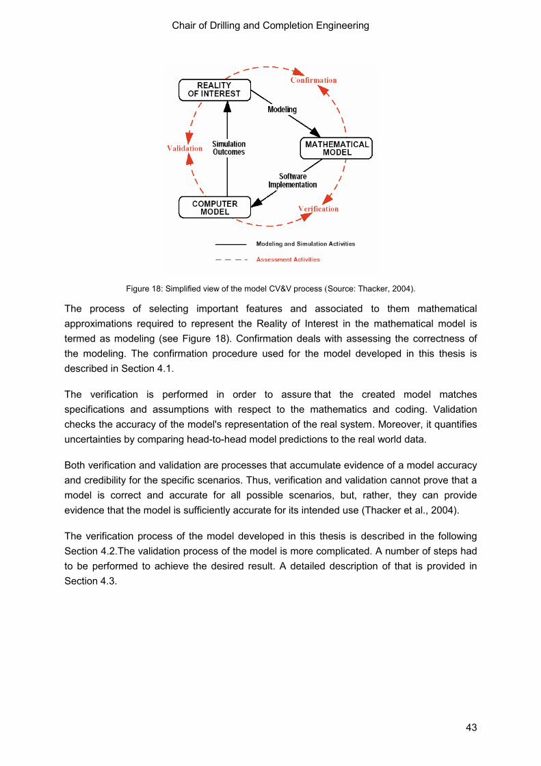
Chair of Drilling and Completion Engineering
43
Figure 18: Simplified view of the model CV&V process (Source: Thacker, 2004).
The process of selecting important features and associated to them mathematical
approximations required to represent the Reality of Interest in the mathematical model is
termed as modeling (see Figure 18). Confirmation deals with assessing the correctness of
the modeling. The confirmation procedure used for the model developed in this thesis is
described in Section 4.1.
The verification is performed in order to assure that the created model matches
specifications and assumptions with respect to the mathematics and coding. Validation
checks the accuracy of the model's representation of the real system. Moreover, it quantifies
uncertainties by comparing head-to-head model predictions to the real world data.
Both verification and validation are processes that accumulate evidence of a model accuracy
and credibility for the specific scenarios. Thus, verification and validation cannot prove that a
model is correct and accurate for all possible scenarios, but, rather, they can provide
evidence that the model is sufficiently accurate for its intended use (Thacker et al., 2004).
The verification process of the model developed in this thesis is described in the following
Section 4.2.The validation process of the model is more complicated. A number of steps had
to be performed to achieve the desired result. A detailed description of that is provided in
Section 4.3.
Chair of Drilling and Completion Engineering
44
4.1 Model Confirmation
To assess the correctness of the developed model a simple approach is taken. The Reality
of Interest and the developed Mathematical Model were taken to different specialists. Each
specialist from a different field provides a specific feedback thus giving the model
Confirmation.
At first, the description and assumptions of the Reality of Interest are checked by an expert to
assure that it represents a Drilling Rig System correctly. With the feedback provided by the
expert, some corrections are made in the assumptions of the Reality of Interest.
At second, the developed Mathematical Model is checked to assure that the conceptual
model, mathematical equations, and modeling data describe the Reality of Interest correctly.
This part is carried out by two experts. The first expert, Dr. Stefan Wirth (OMV) checks the
model to assure that the mathematical model represents the Reality of Interest correctly in
terms of the rig system functions and specifications. The second expert, Dr. Edson Bortoni
(UNIFEI), checks the model to assure that each equipment (e.g. top drive, VFD) is correctly
represented by the calculations, including the mechanical power performed by the
equipment, the motor losses, the VFD losses, and the total electrical input power. All the
necessary corrections are based on the feedback provided by the experts. After that the
Mathematical Model is implemented as a Computer Model using Microsoft Excel. Once the
Computer Model is ready, the verification part of the model can start.
4.2 Model Verification
Model verification is defined as “a process of determining that a model implementation
accurately represents the developer’s conceptual description of the model and the solution to
the model” (AIAA, 1998). In other words, it verifies if the implementation of the model is
accurately accomplished in regards to codes and mathematics. Shortly, verification deals
with the concepts, mathematics and codes of the model. Validation deals with the accuracy
of the results of the model. As concepts, mathematical and code errors can eliminate the
impression of correctness/accuracy (i.e. by giving the right answer for the wrong reason), the
verification process should be realized until a high level of credibility before the validation
activity begins (Thacker et al., 2004).The verification activity of the model developed in this
thesis can be divided into code verification and mathematics verification.
When performing code verification, problems are devised to demonstrate that the code can
compute an accurate solution. Code verification problems are constructed to verify code
correctness, robustness and specific code algorithms. The purpose of code verification is to
confirm that the software is working as intended. The main focus of this activity is to identify
and eliminate programming and implementation errors within the software (software quality
Chair of Drilling and Completion Engineering
45
assurance) and to verify the correctness of the numerical algorithms that are implemented in
the code.
When performing mathematic verification, a model that is to be validated is exercised to
demonstrate that the model is computing a sufficiently accurate solution. The purpose of
calculation verification is to quantify the error of a numerical simulation (Thacker et al., 2004).
4.3 Model Validation
Model validation is defined as the “process of determining the degree to which a computer
model is an accurate representation of the real world from the perspective of the intended
model applications” (AIAA, 1998). It is accomplished through the comparison of predictions
from a model to experimental results (Paez, 2009).
A model should be developed for a specific purpose (or application) and its validity is
determined with respect to its purpose/application. In this thesis the model was developed
with the application of calculating the energy consumed by a drilling rig to drill a shale gas
well in Europe with the use of simulated drilling data. Thus, to validate the model it is
necessary to compare the predictions of energy consumed from the model developed
against experimental results of energy consumed by drilling rigs. Dedicated studies are
performed to understand how it is possible to accomplish this comparison. The studies result
in the comparison between the calculated values of the fuel consumed per day (based on
real drilling data and the input parameters from the drilling rig) against the real values of the
fuel consumed per day (obtained from the drilling morning reports). To accomplish this
comparison two main steps are necessary.
Firstly, it is necessary to transform the predictions from the Energy Consumption Model into
fuel consumed by the rig. This is accomplished by use of a simple mathematical model to
convert the energy consumed by the rig (these are the output results of the model described
in the Chapter 3) into the desired parameter. This model, called “Fuel Consumption Model”,
is described in the following section.
Secondly, it is necessary to obtain all necessary input data to run the models and the real
values of the fuel consumed by the rig, to be able to establish a comparison between the
results. This is done by using real drilling data, all the necessary specification of the
equipment, and the drilling morning report from a real well. The real drilling data (in a 24h
time-span form) and the equipment specification of the rig are used as input. The Energy
Consumption Model provides the total energy consumed by the rig in 24 hours. Further,
using Fuel Consumption Model it is possible to transform the results of energy consumed
into fuel consumed by the rig in 24 hours period.
The validation may then be performed by the comparison of calculated values of daily fuel
consumption against the real values of daily fuel consumptions. The comparisons and

Chair of Drilling and Completion Engineering
46
analysis of the results for several case studies are presented and discussed in the later part
of this section.
4.3.1 Fuel Consumption Model
This section describes the concepts and the mathematical formulations that are used to
simulate the fuel consumption of a drilling rig. The mathematical formulation uses the total
power required by the rig (output from the model described in Chapter 3) and converts it into
consumed fuel. The model simulates mathematically the fuel consumption of the Diesel AC
Generator on the drilling rig. The results generated by this model are presented in the
Section 4.3.2 and Appendix A, where the calculated values of fuel consumption per day are
compared to the real fuel consumption values per day obtained from the drilling morning
reports.
For a coherent description of the developed model, this section is divided into two sub-
sections. The first sub-section defines all input data, which are necessary to run the model.
The second sub-section explains necessary concepts (e.g. fuel rate, fuel consumption) and
equations used to develop the model. The results are presented in gal, gal/h, and gal/day
because all the manufacture data, which is used as input, are obtained in these units. All the
data used in the validation process of the model are obtained from USA companies, thus the
fuel consumption in the morning reports are also obtained in gallons.
4.3.1.1 Input Data
The input data necessary for this model are the information regarding the generators in the
rig. These data summarize all the necessary information to calculate the fuel consumption of
the drilling rig. The input data are:
Electrical rating [kW];
Number of generators;
Fuel consumption for different loads (0%, 25%, 50%, 75% and 100%).
The specifications of the generators for loads at 25%, 50%, 75% and 100% are obtained
from the manufactures of the equipment. At No-Load (0%) the Diesel Consumption will be 10
to 10.2% of the Full Load consumption (Dhayanandhan, 2011). The table below show the
input data is presented in the model.

Chair of Drilling and Completion Engineering
47
Table 9: Generators input data.
Generator Data
Elect. Rating [kW] 1250
Nº Generators 2
Load [%] Fuel Consumption [gal/h]
100% 88.8
75% 65
50% 45.5
25% 26.9
0% 8.88
4.3.1.2 Fuel Consumption Model Description
As described in section 2.5, the generator provides all the energy consumed by the AC
Electrical Drilling Rig. To accomplish that, the diesel engine burns fuel (diesel) to rotate the
generator shaft and produces the electrical energy necessary to perform the job.
As described before, with the constant variation of loads, due to different operations in the
drilling rig, the fuel consumption of the generator also varies. From the manufacturer of the
equipment it is possible to obtain the fuel consumption for the loads 0%, 25%, 50%, 75% and
100% (used for Figure 19). Thus, the first step of the model includes calculation of the fuel
consumption for any load of the generator based on the input data provided by the
manufacturer.
The losses of the diesel generator are captured within the values of fuel consumption by
load. The visualization of these losses is better when analyzing the fuel consumption with a
load of 0% of the generators. The necessary concepts to understand the losses of the
generator are presented in Section 3.2.2.
Figure 19 is a plot where load versus fuel consumption provided by the manufacturer is
shown. A regression line can be drawn to connect the five points. Thus the equation
representing this regression line can describe the fuel consumption for any load of the
generator. Eq. 29 represents the general form of this equation. Figure 19 shows an example
of a graphic of fuel consumption by load of a generator with a regression line and equation.
[ ] [ ] [
]
Eq. 29
where:
- Fuel rate consumption [gal/h];
- Constants.

Chair of Drilling and Completion Engineering
48
Figure 19: Fuel consumption variation by load.
The second step is to transform the total electrical power required by the rig (calculated by
the Energy Consumption Mathematical Model, described in the previous section) into
percentage of the total load of the generator. To accomplish that, the total electric power
required by the rig is divided by the total power installed from the generators.
[ ] Eq. 30
where:
- Total power installed [W].
Applying the load percentage calculated by Eq. 30it is possible to obtain the fuel
consumption per hour from the rig at that instantaneous moment. Using this concept in the
developed model with drilling data it is possible to calculate the fuel consumption related to
the time-span of the data frequency.
[ ] Eq. 31
where:
- Fuel Consumption [gal].
Table 10 presents the continuation of Table 3, which contains drilling data channels with a
sampling frequency of 0.2 Hz. In Table 10the calculated total electrical power required by the
rig is converted into load percentage of the generators. Then, the fuel consumed by the
Rfuel = 14.24x[Load]2 + 64.936x[Load] + 9.208
0
20
40
60
80
100
0% 20% 40% 60% 80% 100% 120%
Fue
l Co
nsu
mp
tio
n [
gal/
l]
Load [%]
Fuel Consumption vs. Load
Fuel Consumption [gal/h]

Chair of Drilling and Completion Engineering
49
generator to generate the required load is calculated based on 5s interval (referent to 0.2 Hz
frequency) of the drilling data.
Table 10: Drilling data used in the model with 0.2 Hz sampling frequency.
Date Time Total Electrical Power [kW]
Load % Fuel Rate [gal/h]
Fuel Consumption
[gal]
14.09.2013 06:00:00 308.78 10.3% 21.00 0.06
14.09.2013 06:00:05 612.45 20.4% 21.00 0.06
14.09.2013 06:00:10 1327.11 44.2% 49.70 0.14
14.09.2013 06:00:15 1549.13 51.6% 56.99 0.16
14.09.2013 06:00:20 1509.38 50.3% 55.69 0.15
14.09.2013 06:00:25 1043.30 34.8% 40.38 0.11
14.09.2013 06:00:30 474.92 15.8% 21.00 0.06
14.09.2013 06:00:35 314.98 10.5% 21.00 0.06
14.09.2013 06:00:40 561.37 18.7% 21.00 0.06
14.09.2013 06:00:45 964.78 32.2% 37.80 0.10
14.09.2013 06:00:50 1061.73 35.4% 40.98 0.11
14.09.2013 06:00:55 1037.47 34.6% 40.18 0.11
14.09.2013 06:01:00 468.69 15.6% 21.00 0.06
The sum of the fuel consumptions for a period of 24 hours gives the amount of fuel
consumed by the rig in one day. Thus, if real drilling data is used to feed the Energy
Consumption Mathematical Model the results of the fuel consumption for the periods of 24
hours can be obtained. After, the result is compared with the real values of fuel consumed by
the rig. This analysis is presented in the following section.
4.3.2 Model Predictions vs. Measured Data
To accomplish the validation of the model several wells are selected from the data base.
Careful studies are performed to ensure that selected wells have all necessary input data for
the models and the real values of fuel consumed by the rig for the further comparison
(validation).
This section presents the comparison of results, for one well, of the calculated values of fuel
consumed based on the real input data and the real values of fuel consumed daily by the
drilling rig extracted from the drilling morning reports.
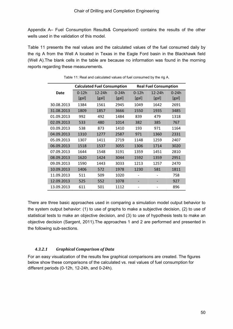
Chair of Drilling and Completion Engineering
50
Appendix A– Fuel Consumption Results& Comparison 0 contains the results of the other
wells used in the validation of this model.
Table 11 presents the real values and the calculated values of the fuel consumed daily by
the rig A from the Well A located in Texas in the Eagle Ford basin in the Blackhawk field
(Well A).The blank cells in the table are because no information was found in the morning
reports regarding these measurements.
Table 11: Real and calculated values of fuel consumed by the rig A.
Date
Calculated Fuel Consumption Real Fuel Consumption
0-12h [gal]
12-24h [gal]
0-24h [gal]
0-12h [gal]
12-24h [gal]
0-24h [gal]
30.08.2013 1384 1561 2945 1049 1642 2691
31.08.2013 1809 1857 3666 1550 1935 3485
01.09.2013 992 492 1484 839 479 1318
02.09.2013 533 480 1014 382 385 767
03.09.2013 538 873 1410 193 971 1164
04.09.2013 1310 1277 2587 971 1360 2331
05.09.2013 1307 1411 2719 1148 1259 2407
06.09.2013 1518 1537 3055 1306 1714 3020
07.09.2013 1644 1548 3191 1359 1451 2810
08.09.2013 1620 1424 3044 1592 1359 2951
09.09.2013 1590 1443 3033 1213 1257 2470
10.09.2013 1406 572 1978 1230 581 1811
11.09.2013 511 509 1020 - - 758
12.09.2013 525 552 1078 - - 927
13.09.2013 611 501 1112 - - 896
There are three basic approaches used in comparing a simulation model output behavior to
the system output behavior: (1) to use of graphs to make a subjective decision, (2) to use of
statistical tests to make an objective decision, and (3) to use of hypothesis tests to make an
objective decision (Sargent, 2011).The approaches 1 and 2 are performed and presented in
the following sub-sections.
4.3.2.1 Graphical Comparison of Data
For an easy visualization of the results few graphical comparisons are created. The figures
below show these comparisons of the calculated vs. real values of fuel consumption for
different periods (0-12h, 12-24h, and 0-24h).

Chair of Drilling and Completion Engineering
51
Appendix A– Fuel Consumption Results& Comparison contains the graphical comparison of
the result from other wells used in the model validation. Figure 20 presents the calculated
and real values of fuel consumed in the period of 0 to 12 hours. The ordinate axis contains
the daily fuel consumption values and the abscissa contains the time span of the well.
Figure 20: Real Fuel vs. Calculated Fuel Consumption referent to the period of 0-12h.
Figure 21 presents the same type of graphic as in Figure 20, with the difference that the
calculated and real values of fuel consumed are referring to the period of 12 to 24 hours. The
discontinuity of the red line for the last three days in both of first two figures is due to the
blank cells in the Table 11, caused by the lack of information in the morning reports.
Figure 21: Real Fuel vs. Calculated Fuel Consumption referent to the period of 12-24h.
Figure 22 presents the same type of graphic as in the figures above, with the difference that
the calculated and real values of fuel consumed are referring to the period of one full day.
0
200
400
600
800
1000
1200
1400
1600
1800
Fuel
Co
nsu
mp
tio
n [
gal/
day
] Real Fuel vs. Calculated Fuel Consumption 0-12h
Calculated Fuel Consumption Real Fuel Consumption
0
200
400
600
800
1000
1200
1400
1600
1800
2000
Fuel
Co
nsu
mp
tio
n [
gal/
day
]
Real Fuel vs. Calculated Fuel Consumption 12-24h
Calculated Fuel Consumption Real Fuel Consumption

Chair of Drilling and Completion Engineering
52
By analyzing these graphics it is possible to observe a good correlation between the results.
This correlation gives to the developed model a first credibility. The graphic comparison is
not enough for validation of the model because it is a subjective analysis. Thus, more
objective analysis needs to be performed with the use of statistical test in order to assure
accuracy and credibility of the model.
Figure 22:Real Fuel vs. Calculated Fuel Consumption referent to the period of 0-24h.
4.3.2.2 Coefficient of Determination - R2
Literature studies are made in order to understand what types of statistical tests can be
performed with the available data. The coefficient of determination (R2) is chosen as suitable
statistical tool to make an objective decision of the accuracy and credibility of the developed
model.
In statistics, the coefficient of determination, denoted as R2 and pronounced R squared,
provides an estimate of the proportion of overlapping variance between two sets of numbers
(i.e., the degree to which the two sets of numbers vary together), it indicates how well data
points fit a line or curve (Brown, 2003). It is a statistic tool used in this thesis with the main
purpose to provide a measure of how well the calculated fuel consumption values are
correlated with the real fuel consumed values.
Coefficient of determination can take values as high as 1 when all the values are completely
correlated, or as low as 0 when all the values are different (i.e. 0≤R2≤1). In Figure 23 a
scatter plot is presented, where the real fuel consumption values are plotted against the
calculated fuel consumption values of the model for the Well A. A regression line is
presented in the plot, and since the relation between the real fuel consumption values and
the calculated fuel consumption values is linear, the regression line is forced through zero.
The slope of the straight line shows the average ratio between the calculated values in
relation to the real values. The closer the slope to 45°, the more precise the calculated
0
500
1000
1500
2000
2500
3000
3500
4000
Fuel
Co
nsu
mp
tio
n [
gal/
day
]
Real Fuel vs. Calculated Fuel Consumption 0-24h
Calculated Fuel Consumption Real Fuel Consumption
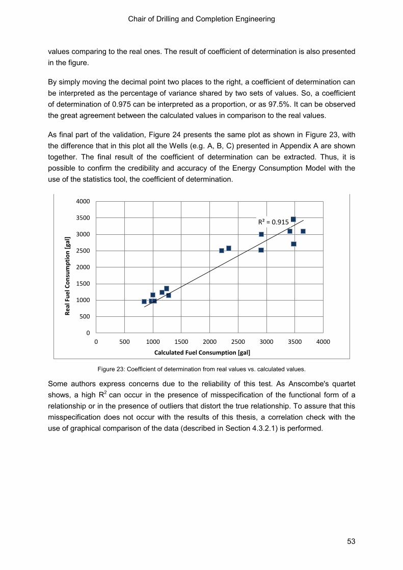
Chair of Drilling and Completion Engineering
53
values comparing to the real ones. The result of coefficient of determination is also presented
in the figure.
By simply moving the decimal point two places to the right, a coefficient of determination can
be interpreted as the percentage of variance shared by two sets of values. So, a coefficient
of determination of 0.975 can be interpreted as a proportion, or as 97.5%. It can be observed
the great agreement between the calculated values in comparison to the real values.
As final part of the validation, Figure 24 presents the same plot as shown in Figure 23, with
the difference that in this plot all the Wells (e.g. A, B, C) presented in Appendix A are shown
together. The final result of the coefficient of determination can be extracted. Thus, it is
possible to confirm the credibility and accuracy of the Energy Consumption Model with the
use of the statistics tool, the coefficient of determination.
Figure 23: Coefficient of determination from real values vs. calculated values.
Some authors express concerns due to the reliability of this test. As Anscombe's quartet
shows, a high R2 can occur in the presence of misspecification of the functional form of a
relationship or in the presence of outliers that distort the true relationship. To assure that this
misspecification does not occur with the results of this thesis, a correlation check with the
use of graphical comparison of the data (described in Section 4.3.2.1) is performed.
R² = 0.915
0
500
1000
1500
2000
2500
3000
3500
4000
0 500 1000 1500 2000 2500 3000 3500 4000
Re
al F
ue
l Co
nsu
mp
tio
n [
gal]
Calculated Fuel Consumption [gal]

Chair of Drilling and Completion Engineering
54
Figure 24: General coefficient of determination for the Energy Consumption Model.
4.4 Accreditation
The definition of accreditation provided by the USA Department of Defense is the following:
“official certification that a model, simulation, or federation of models and simulations and its
associated data are acceptable for use for a specific application”. Thus, the process of CV&V
developed in this thesis assures the accreditation of the Energy Consumption Model.
As a final step to describe the exactly model development and CV&V process, Figure 25 is
created. Figure 25 expands Figure 18, providing more detailed description of the whole
process. Although Figure 18 is effective for explaining the major concepts involved in the
CV&V model, several important activities are not shown. Figure 18 does not clearly represent
1) the various activities performed in the development of the model; 2) each process
outcome achieved; and 3) an objective process for improving agreement between real data
and the calculated data.
In Figure 25, the right branch illustrates the process of developing and exercising the model,
and the left branch illustrates the process of obtaining relevant and high quality data to serve
as input to the model and to accomplish the validation of the same. The closed boxes are the
direct results of the process activities called process outcome. The connectors in black solid
lines denote certain activities as to go from one outcome to the next. The connectors in
dashed red lines mean the activities perform to evaluate the model and are called
assessment activities.
R² = 0.941
0
500
1000
1500
2000
2500
3000
3500
4000
0 500 1000 1500 2000 2500 3000 3500 4000
Re
al F
ue
l Co
nsu
mp
tio
n [
gal]
Calculated Fuel Consumption [gal]

Chair of Drilling and Completion Engineering
55
Reality of Interest
Conceptual Model
Mathematical Model
Computer Model
Caculated Fuel Consumed
Values
Acceptable Agreement?
Model Accepted
Real Fuel Consumed
Values
Real Data Acquisition
Quantitative Comparison
Revise Model
Mathematical Modeling
Implementation
Simulation
Yes
No
Abstration
Model Validation
Code & Mathematic Verification
Model Confirmation
Database
Data QC
Input Data
Drilling Chan. & Rig Spec.
Data Export
Assessment Activities
Process Activities
Process Outcome
Figure 25: Detailed model development and CV&V. (Source: Modified from Thacker, 2004).

Chair of Drilling and Completion Engineering
56
5. Conclusion
This chapter concludes the thesis with obtained results, difficulties/complications
encountered during the thesis, and a short summary of the key recommendations for future
applications. These recommendations were developed during the research based on the
knowledge gathered.
1) The validation results of the developed energy consumption model confirm that the energy
consumption of the top drive, mud pump and draw-works represent 88-95% of total daily
drilling rig energy consumption. The mud circulation system takes the largest percentage of
this energy use in the rig operation, thus improving the efficiency of the mud circulation
system generates the highest impact on overall energy consumed. All the other equipment at
the rig site (e.g. light, air conditioning system) consumes the remaining 12-5%.
2) Drilling data/parameters management: it was quite easy to obtain necessary data from the
drilling channels (as they are common drilling parameters), although it was challenging to get
correct specifications of the drilling rig equipment. Additionally, a drilling data quality check
had to be performed in order to assure their sufficient quality.
3) As the inconsistent results of energy consumption were obtained due to incorrect
information on the equipment power rating, the importance of the correct equipment power
rating was noticed.
4) Significance of differentiating tripping-in and tripping-out operations was noticed for the
energy consumption model of draw-works. During tripping-in operations the draw-works use
only brakes when lowering the drill string, thus, only a fixed amount of power is required.
During tripping-out operations the draw-works require power to lift the complete hookload of
the system at a certain speed.
5) Moreover, it was noticed that the information on number of sheaves in the crown
block/traveling block is not required for calculation of the mechanical power of the draw-
works, as explained in Section 3.3.3.2.
6) Based on the comparison of real vs. calculated figures of fuel consumption, the conceptual
model was incrementally refined and improved. As a final figure the author obtained an R2 of
overall 94.1% of all the data used for the model validation.
As a final statement for the scope of this study, the thesis was a success since the objectives
of the thesis were achieved. During the research, great understanding on the energy supply
and energy consumption of a drilling rig was gained, as well as the specific knowledge on
how to develop a model starting from the definition of the Reality of Interest until the Model
Accreditation.
For future development and application of the research, the author recommends a more
detailed analysis, which can be focused on:

Chair of Drilling and Completion Engineering
57
1) to develop Energy (Energy efficiency) Based KPIs. The results of the energy
consumption model combined with the rig states generated by the Automatic State
Recognition system could define the energy consumed for each state. Further these
states are combined in KPIs, thus providing the total energy consumed for each of
the measured KPIs. Studies will be necessary to better understand the application of
the results.
2) to create an operations breakdown according to energy demand of a future well
based on a Drilling Data Simulator.
3) to use the total mechanical power output to quality check the drilling data: this value
must never be greater than the equipment power rating specification.
4) to get more extensive set of Rig specifications to facilitate further study;
5) to use the Energy Based KPIs in order to quantify the amount of CO2, NO2 emission
for each operation and create a comparison of the emissions for different sources of
energy (e.g. electrical power grid, diesel motors, among others).

Chair of Drilling and Completion Engineering
58
6. Bibliography
AIAA. (1998). Guide for the Verification and Validation of Computational Fluid Dynamics
Simulations. Reston: AIAA-G-077-1998.
Al-Morakhi, R., Al-Shemali, A., Alsammak, I., Esterabadi, J., Martocchia, A., Ferroni, G., et al.
(2013, 10 10). Real Time Advanced Flow Analysis for Early Kick/Loss Detection &
Identification of Open Fractures. SPE Kuwait Oil and Gas Show and Conference.
SPE-167335-MS, p. 6. Mishref, Kuwait: SPE.
Arnaout, A., Zoellner, P., Johnstone, N., & Thonhauser, G. (2013). Intelligent Data Quality
Control of Real-time Rig Data. SPE Middle East Intelligent Energy Conference and
Exihibition (p. 9). Dubai: SPE International.
Australian, D. o. (2008). Mechanical & Electrical power relationships. Brisbane: Australian
Flexible Learning Framework.
Automation Consulting, LLC. (2011, 11 27). Variable Frequency Drives (VFDs). Nashville,
Tennessee, USA. Retrieved from http://automationprimer.com/2011/11/27/variable-
frequency-drives-vfds/
Azar, J. J., & Samuel, G. R. (2007). Drilling Engineering. Tulsa: PennWell Corporation.
Bentec Ltd. (2013). Product information. Retrieved 11 21, 2013, from Bentec Ltd.:
http://www.bentec.com/equipment/mechanical-products/
Besore, S. (2010, 09 08). MTU Detroit Diesel. Retrieved 11 30, 2013, from Drilling
Contractor: http://www.drillingcontractor.org/fuel-consumption-overload-capacity-
among-critical-criteria-in-selection-of-generator-sets-6864
Bonitron Inc. (2014). Retrieved 11 21, 2014, from Bonitron Inc.:
http://www.bonitron.com/industry-oil-drawworks.html
Brown, J. D. (2003, 03 1). The coefficient of determination. Manoa, Hawai, USA. Retrieved
from http://jalt.org/test/bro_16.htm
Burt, C., Piao, X., Gaudi, F., Busch, B., & Taufik, N. (2006). Electrical Motor Efficiency under
Variable Frenquencies and Loads. San Luiz Obispo: Irrigation Training & Research
Center.
Cherutich, S. K. (2009). Rig Selection and Comparison of Top Drive and Rotary Table Drive
Systems for Cost Effective Drilling Preject in Kenya. Naivasha: Kenya Electricity
Generating Co, Ltd – KenGen.
China-OGPE. (2013). Retrieved 11 21, 2014, from China Manufacturers and Suppliers of Oil,
Gas and Petrochemical Equipment: http://www.china-ogpe.com/
Dhayanandhan, G. (2011, 02 27). Calculating Consumption for a Diesel Generator. CHENNI,
TAMIL NADU, INDIA. Retrieved from http://cr4.globalspec.com/thread/76597
Diesel Service & Supply. (2013). Approximate Diesel Fuel Consumption Chart. Retrieved
from http://www.dieselserviceandsupply.com/Diesel_Fuel_Consumption.aspx

Chair of Drilling and Completion Engineering
59
DrillingFormula. (2010, 04 10). Drilling Formulas. Retrieved 11 25, 2013, from Frictional
Pressure Loss Components in the Rig Circulating System:
http://www.drillingformulas.com/frictional-pressure-loss-components-in-the-rig-
circulating-system/
Florence, F., & Iversen, F. (2010). Real-time models for drilling process automation:
Equations and applications. IADC/SPE Drilling Conference and Exhibition.
GlobalSpec Inc. (2013). Retrieved 01 12, 2015, from IHS GlobalSpec:
http://www.globalspec.com/
Heinemann, Z. E. (2005). Fluid Flow in Porous Media. Leoben: Montanuniversität.
Lyons, W. C. (1996). Standard Handbook od Petroleum & Natural Gas Engineering.
Houston: Gulf Publishing Company.
Mathis, W., & Thonhauser, G. (2007). Mastering Real-Time Data Quality Control - How To
Measure and Manage the Quality of (Rig) Sensor Data. Middle East Drilling
Technology Conference & Exihibition (p. 10). Cairo: SPE/IADC.
McCoy, G. A., Litman, T., & Douglass, J. G. (1993). Energy-Efficient Electric Motor Selection
Handbook. Olympia,: Washington State Energy Office.
NOV. (2014). Retrieved 01 12, 2015, from National Oilwell Varco:
http://www.nationaloilwell.com/
Oil & Gas Journal. (2006, 02 20). Retrieved 11 24, 2014, from Oil & Gas Journal:
http://www.ogj.com/articles/print/volume-104/issue-7/special-report/nabors-drilling-
designs-new-ac-rigs.html
Paez, T. L. (2009). Introduction to Model Validation. IMAC-XXVII. Orlando: Society for
Experimental Mechanics Inc.
Prassl, W. F. (2002). Drilling Engineering. Curtin: Curtin University of Technology.
Rajput, R. (1998). A Textbook of Hydraulic Machines in SI Units. New Delhi: S. Chand &
Company Pvt.
Rigmaster Machinery Ltd. (2013). Retrieved 01 12, 2015, from RigMaster:
http://www.rigmastermachinery.com/index.php?id=65
Saidur, R. (2009, 10 20). A review on electrical motors energy use and energy savings.
Renewable and Sustainable Energy Reviews, pp. 877-898.
Sargent, R. G. (2011). Verification and Validation of Simulation Models. Winter Simulation
Conference. Phoenix: Institute of Electrical and Electronics Engineers.
Schlumberger. (2012). The Expanding Role of Mud Logging. Oilfield Review.
Singh, S. K. (2003). Industrial Instrumentation & Control - 2 ed. New Delhi: Tata McGraw-Hill
Publishing Company Limited.
Sivasankaran, G. A., & Jain, S. (1988, July). Performance of Diesel Engines at High
Altitudes. Def Sci J, Vol 38, No. 3, pp. pp. 301-313.

Chair of Drilling and Completion Engineering
60
Sola, A. V., & Mota, C. M. (2011, 12 17). A multi-attribute decision model for portfolio
selection aiming to replace technologies in industrial motor systems. Energy
Conversion and Management, pp. 97-106.
Thacker et al., B. H. (2004). Concepts of Model Verification and Validation. Los Alamos: Los
Alamos National Laboratory.
Waide, P., & Brunner, C. U. (2011). Energy-Efficiency Policy Opportunities for Electric Motor-
Driven Systems. Paris: International Energy Agency.

Chair of Drilling and Completion Engineering
61
Appendix A– Fuel Consumption Results& Comparison
This appendix contains the results of the calculated values of fuel consumed based on the
real input data and the real values of fuel consumed daily by the drilling rig extracted from the
drilling morning reports for all the other wells used to validate this model.
Well B
Date
Calculated Fuel Consumption Real Fuel Consumption
0-12h [gal]
12-24h [gal]
0-24h [gal]
0-12h [gal]
12-24h [gal]
0-24h [gal]
30.08.2013 450 486 937 - 767 1149
31.08.2013 976 976 1952 - 796 2101
01.09.2013 964 940 1904 - - -
02.09.2013 546 510 1055 - 471 1439
03.09.2013 1236 1273 2509 - 1360 2898
04.09.2013 1249 1308 2557 - 2617 2617
05.09.2013 1444 1175 2619 - - -
06.09.2013 1283 1444 2727 - - 2909
07.09.2013 1391 1448 2839 - - 2962
08.09.2013 1313 493 1807 - - 2299
09.09.2013 370 446 816 - - 972
10.09.2013 1284 1530 2815 - - 2719
11.09.2013 1529 1155 2684 - - 2978
12.09.2013 435 423 858 - - 1020
13.09.2013 428 447 875 - - 1159
14.09.2013 411 365 776 - - 956
0
500
1000
1500
2000
2500
3000
3500
Fuel
Co
nsu
mp
tio
n [
gal/
day
]
Real Fuel vs. Calculated Fuel Consumption 0-24h
Calculated Fuel Consumption Real Fuel Consumption

Chair of Drilling and Completion Engineering
62
Well C
Date
Calculated Fuel Consumption Real Fuel Consumption
0-12h [gal]
12-24h [gal]
0-24h [gal]
0-12h [gal]
12-24h [gal]
0-24h [gal]
10.09.2013 377 1128 1505 572 1002 1574
11.09.2013 1629 1874 3503 1698 1991 3689
12.09.2013 1322 1426 2748 1303 1706 3009
13.09.2013 1846 971 2817 1779 1118 2897
14.09.2013 397 418 816 472 491 963
15.09.2013 377 403 780 409 468 877
16.09.2013 671 1220 1891 732 1199 1931
R² = 0.949
0
500
1000
1500
2000
2500
3000
3500
0 500 1000 1500 2000 2500 3000
Re
al F
ue
l Co
nsu
mp
tio
n [
gal]
Calculated Fuel Consumption [gal]
0
500
1000
1500
2000
2500
3000
3500
4000
Fuel
Co
nsu
mp
tio
n [
gal/
day
]
Real Fuel vs. Calculated Fuel Consumption 0-24h
Calculated Fuel Consumption Real Fuel Consumption

Chair of Drilling and Completion Engineering
63
Well D
Date
Calculated Fuel Consumption Real Fuel Consumption
0-12h [gal]
12-24h [gal]
0-24h [gal]
0-12h [gal]
12-24h [gal]
0-24h [gal]
07.08.2013 1178 1318 2496 1344 1230 2574
08.08.2013 1294 639 1933 2072 193 2265
09.08.2013 1021 1220 2242 1060 1115 2175
10.08.2013 1184 1277 2461 1479 949 2428
11.08.2013 1386 1421 2807 1549 1164 2713
12.08.2013 1466 914 2380 1723 776 2499
13.08.2013 606 520 1126 778 387 1165
R² = 0.995
0
500
1000
1500
2000
2500
3000
3500
4000
0 500 1000 1500 2000 2500 3000 3500 4000
Re
al F
ue
l Co
nsu
mp
tio
n [
gal]
Calculated Fuel Consumption [gal]
0
500
1000
1500
2000
2500
3000
Fuel
Co
nsu
mp
tio
n [
gal/
day
]
Real Fuel vs. Calculated Fuel Consumption 0-24h
Calculated Fuel Consumption Real Fuel Consumption

Chair of Drilling and Completion Engineering
64
Well E
Date
Calculated Fuel Consumption Real Fuel Consumption
0-12h [gal]
12-24h [gal]
0-24h [gal]
0-12h [gal]
12-24h [gal]
0-24h [gal]
20.07.2013 754 621 1375 - - 1612
21.07.2013 447 446 893 - - -
22.07.2013 412 412 824 - - -
23.07.2013 419 421 839 - - -
24.07.2013 621 1208 1829 582 1166 1748
25.07.2013 966 1210 2175 765 1160 1925
26.07.2013 1371 1116 2487 1553 1333 2886
27.07.2013 471 1058 1529 574 1166 1740
28.07.2013 1240 1348 2588 933 1537 2470
29.07.2013 1388 1478 2865 1070 1505 2575
30.07.2013 1358 802 2161 1334 772 2106
31.07.2013 531 845 1376 521 721 1242
01.08.2013 1318 1376 2693 1273 1305 2578
02.08.2013 630 481 1110 527 727 1254
03.08.2013 510 519 1029 560 569 1129
R² = 0.916
0
500
1000
1500
2000
2500
3000
3500
0 500 1000 1500 2000 2500 3000
Re
al F
ue
l Co
nsu
mp
tio
n [
gal]
Calculated Fuel Consumption [gal]

Chair of Drilling and Completion Engineering
65
Well F
Date
Calculated Fuel Consumption Real Fuel Consumption
0-12h [gal]
12-24h [gal]
0-24h [gal]
0-12h [gal]
12-24h [gal]
0-24h [gal]
17.08.2013 449 830 1280 - - 1146
18.08.2013 1066 1273 2338 - - 2573
19.08.2013 1327 888 2215 - - 2510
20.08.2013 493 507 999 - - 1160
21.08.2013 428 422 849 - - 953
22.08.2013 481 682 1163 - - 1230
23.08.2013 1442 1469 2910 - - 2997
0
500
1000
1500
2000
2500
3000
3500
Fuel
Co
nsu
mp
tio
n [
gal/
day
] Real Fuel vs. Calculated Fuel Consumption 0-24h
Calculated Fuel Consumption Real Fuel Consumption
R² = 0.873
0
500
1000
1500
2000
2500
3000
3500
0 500 1000 1500 2000 2500 3000 3500
Re
al F
ue
l Co
nsu
mp
tio
n [
gal]
Calculated Fuel Consumption [gal]

Chair of Drilling and Completion Engineering
66
24.08.2013 1614 2037 3651 - - 3088
25.08.2013 1813 6040 7853* - - -
26.08.2013 2262 1218 3481 - - 2707
27.08.2013 1381 1527 2908 - - 2522
28.08.2013 1702 1709 3411 - - 3088
29.08.2013 1700 1773 3473 - - 3455
30.08.2013 750 492 1242 - - 1351
31.08.2013 439 534 973 - - 973
01.09.2013 555 470 1025 - - 966
* This value clearly shows an error in the drilling data used to calculate the fuel
consumption.
0
500
1000
1500
2000
2500
3000
3500
4000
Fuel
Co
nsu
mp
tio
n [
gal/
day
]
Real Fuel vs. Calculated Fuel Consumption 0-24h
Calculated Fuel Consumption Real Fuel Consumption
R² = 0.915
0
500
1000
1500
2000
2500
3000
3500
4000
0 500 1000 1500 2000 2500 3000 3500 4000
Re
al F
ue
l Co
nsu
mp
tio
n [
gal]
Calculated Fuel Consumption [gal]

Chair of Drilling and Completion Engineering
67
Well G
Date
Calculated Fuel Consumption Real Fuel Consumption
0-12h [gal]
12-24h [gal]
0-24h [gal]
0-12h [gal]
12-24h [gal]
0-24h [gal]
19.06.2013 787 378 1165 - - 1537
20.06.2013 365 363 728 - - 973
21.06.2013 364 364 727 - - 772
22.06.2013 367 521 888 - - 957
23.06.2013 990 1069 2059 - - 2125
24.06.2013 1251 1231 2481 - - 2599
25.06.2013 1218 421 1639 - - 2115
26.06.2013 402 433 836 - - -
27.06.2013 367 364 731 - - -
28.06.2013 364 394 758 - - 927
29.06.2013 513 3299 - - - -
30.06.2013 1466 4108 - - - -
01.07.2013 1225 2960 - - - -
02.07.2013 2137 505 2642 - - -
03.07.2013 378 554 932 - - 970
04.07.2013 555 519 1074 - - 1359
05.07.2013 691 404 1096 - - 1423
06.07.2013 364 373 737 - - -
07.07.2013 602 654 1256 - - 1505
08.07.2013 400 429 829 - - 950
09.07.2013 408 445 853 - - 973
10.07.2013 394 563 957 - - 969
11.07.2013 565 1056 1621 - - 1818
12.07.2013 564 474 1038 - - 1677
13.07.2013 1137 1145 2282 - - 2192
14.07.2013 783 406 1189 - - -
15.07.2013 401 895 1296 - - -
16.07.2013 1203 1184 2387 - - -
17.07.2013 1193 1206 2399 - - 2663
18.07.2013 1152 1246 2397 - - 2417
19.07.2013 716 433 1149 - - -
20.07.2013 1047 1277 2324 - - -
21.07.2013 1272 1298 2569 - - 2494
22.07.2013 817 1327 2145 - - 2520
23.07.2013 1343 1193 2536 - - 2782

Chair of Drilling and Completion Engineering
68
0
500
1000
1500
2000
2500
3000
Fuel
Co
nsu
mp
tio
n [
gal/
day
] Real Fuel vs. Calculated Fuel Consumption 0-24h
Calculated Fuel Consumption Real Fuel Consumption
R² = 0.911
0
500
1000
1500
2000
2500
3000
3500
0 500 1000 1500 2000 2500 3000
Re
al F
ue
l Co
nsu
mp
tio
n [
gal]
Calculated Fuel Consumption [gal]
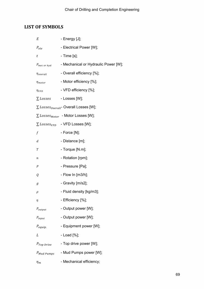
Chair of Drilling and Completion Engineering
69
LIST OF SYMBOLS
- Energy [J];
- Electrical Power [W];
- Time [s];
- Mechanical or Hydraulic Power [W];
- Overall efficiency [%];
- Motor efficiency [%];
- VFD efficiency [%];
∑ - Losses [W];
∑ - Overall Losses [W];
∑ - Motor Losses [W];
∑ - VFD Losses [W];
- Force [N];
- Distance [m];
- Torque [N.m];
- Rotation [rpm];
- Pressure [Pa];
- Flow In [m3/h];
- Gravity [m/s2];
- Fluid density [kg/m3];
- Efficiency [%];
- Output power [W];
- Output power [W];
- Equipment power [W];
- Load [%];
- Top drive power [W];
- Mud Pumps power [W];
- Mechanical efficiency;

Chair of Drilling and Completion Engineering
70
- Hydraulic efficiency;
- Volumetric efficiency;
- Friction efficiency;
- Specific work from the pump or fan [W];
- Specific work lost due to hydraulic effects [W];
- Power transferred from the motor to the shaft [W];
- Power lost in the transmission [W];
- Volume flow out of the pump or fan [W];
- Leakage volume flow [W];
- Fast line linear velocity [m/s];
- Block height [m];
- Time difference [s];
- Number of sheaves;
- Angular velocity [rpm];
- Drum radius [m];
- Hookload [kg];
- Draw-works power [W];
- Extra equipment power [W];
- Total power installed [W];
- Extra equipment load [%];
- Total electrical power [W];
- Fuel rate consumption [gal/h];
- Constants;
- Total power installed [W];
- Fuel Consumption [gal].