The University of Western Australia

School of Electrical, Electronic and Computer Engineering

Development of a Navigation Control System foran Autonomous Formula SAE-Electric Race Car

Thomas H. Drage

20510505

Final Year Project Thesis submitted for the degree of Bachelor of Engineering.

Submitted 1st November 2013

Supervisor: Professor Dr. Thomas Bräunl

Abstract

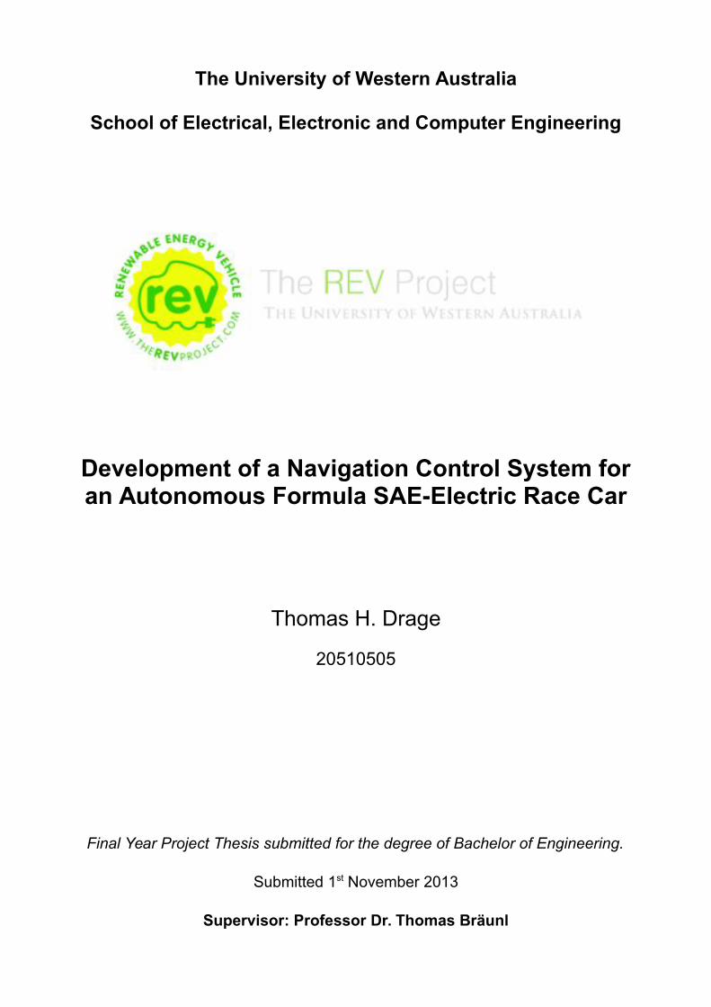
Figure 1: Autonomous Formula SAE-Electric Car

This dissertation describes the development of a high level control system for an autonomous

Formula SAE race car featuring fusion of a 6-DOF IMU, a consumer grade GPS and an automotive

LIDAR. Formula SAE is a long-running annual competition organised by the Society of

Automotive Engineers which has recently seen the introduction of the new class SAE-Electric. The

car discussed in this dissertation features electric motors driving each of the two rear wheels via

independent controllers and has full drive-by-wire control of the throttle, steering and (hydraulic)

braking system. Whilst autonomous driving is outside the scope of the Formula-SAE competition, it

has been the subject of significant research interest over the last several decades. It is intended that

the Autonomous SAE car developed in this project will provide UWA with a platform for research

into driverless performance cars.

This project consists of the design and implementation of a navigation control system which uses a

Linux PC to interface with a range of sensors as well as the drive-by-wire system, safety systems

and a base station. The navigation control system is implemented as a multi-threaded C++ program

featuring asynchronous communication with hardware outputs, sensor inputs and user interfaces.

The Autonomous SAE Car can drive following a map consisting of “waypoints” and “fence posts”

which are recorded by either driving the course manually or through a GoogleMaps based web

interface. Mapped driving is augmented by the use of a LIDAR scanner for detection of obstacles

including road edges for which a novel algorithm is presented. GPS is used as the primary

navigation aid; however sensor fusion algorithms have been implemented in order to improve upon

the measurement of the cars position and orientation through the use of a 6-DOF Inertial

Measurement Unit.

i

Attention to safety is essential in such a project as the car weighs in excess of 250kg and is capable

of driving at a speed of 80km/h. Safety systems are implemented as part of the navigation controller

as well as through independent hardware. Facilities for remote intervention and emergency stopping

are provided through a wireless link to the base station as well as through hard-wired systems on the

car itself.

Measurements derived from autonomous test driving as well as the sensor fusion and road-edge

detection algorithms are presented as well as an overview of the future potential of the platform as a

research tool.

ii

Acknowledgements

I would like to thank the following people for their assistance in this project:

Prof. Thomas Bräunl for his guidance, advice and commitment to the REV Project.

The REV Autonomous SAE Team for their invaluable assistance and camaraderie.

My friends and family for their support and encouragement over the course of this year.

John Cooper and the team at EV Works who have provided us with advice and assistance

with manufacturing parts.

Galaxy Resources, Altronics and Swan Energy for their generous donations to the REV

Project.

Western Power for the support of their undergraduate scholarship programme.

See Appendix A for acknowledgement of the authors of software libraries used in this project.

iii

Nomenclature

AJAX Asynchronous JavaScript and XML

API Application Programming Interface

ARM Advanced/Acorn RISC (Reduced Instruction Set Computer) Machine

NO Normally Open

NC Normally Closed

BMS Battery Management System

COM (Microsoft) Component Object Model

FIFO First In, First Out

GPS Global Positioning System

HTML Hypertext Markup Language

HTTP Hypertext Transfer Protocol

IC Integrated Circuit

IO Input/Output

INS Inertial Navigation System

IMU Inertial Measurement Unit

JSON JavaScript Object Notation

LIDAR Light Detection and Ranging

NMEA National Marine Electronics Association

POSIX Portable Operating System Interface

RAM Random Access Memory

TTL Transistor-Transistor Logic

UART Universal Asynchronous Receiver/Transmitter

USB Universal Serial Bus

UI User Interface

SAE Society of Automotive Engineers

SLA Sealed Lead Acid

WDT Watchdog Timer

Wifi Wireless Local Area Network (e.g. IEEE 802.11)

iv

Table of Contents

Abstract.................................................................................................................................................i Acknowledgements............................................................................................................................iii Nomenclature.....................................................................................................................................iv 1 Introduction and Background...........................................................................................................1

1.1 Introduction...............................................................................................................................1 1.2 Motivation.................................................................................................................................2

2 Literature Review.............................................................................................................................3 3 System Design..................................................................................................................................5

3.1 Overview and Requirements.....................................................................................................5 3.2 Hardware Framework...............................................................................................................6 3.3 Communication and Integration...............................................................................................8 3.4 Software Framework.................................................................................................................9

Navigation Control Program......................................................................................................9 Base Station Hardware IO Software........................................................................................12 Web Interface...........................................................................................................................13

4 Sensor Selection and Integration....................................................................................................14 4.1 Overview.................................................................................................................................14 4.2 Position and Orientation.........................................................................................................15

Global Positioning System.......................................................................................................15 Inertial Measurement Unit.......................................................................................................17 Sensor Fusion...........................................................................................................................18

Vehicle Heading...................................................................................................................19Positioning............................................................................................................................22

4.3 Physical Environment.............................................................................................................24 IBEO LIDAR...........................................................................................................................24 Road Edge Detection...............................................................................................................25 Mapping of Obstacles..............................................................................................................31

5 Instrumentation and Control...........................................................................................................33 5.1 Mapping..................................................................................................................................33

Geodesy....................................................................................................................................33 Implementation........................................................................................................................34

5.2 Trajectory Calculation and Driving........................................................................................34 Overview..................................................................................................................................34 Heading....................................................................................................................................35

Simple Steering Algorithm...................................................................................................35Improved Steering Algorithm...............................................................................................37

Speed........................................................................................................................................38 5.3 User Interfaces........................................................................................................................39

Base Station Driven.................................................................................................................40Base Station Hardware Interface..........................................................................................40Web Interface........................................................................................................................40

Self Contained Operation.........................................................................................................42 6 Safety..............................................................................................................................................43

6.1 Requirements and Design.......................................................................................................43 Risk Assessment.......................................................................................................................43 System Design..........................................................................................................................44

v

6.2 Integrated Safety Features......................................................................................................45 6.3 Hardware Safety Supervisor...................................................................................................47

Hardware..................................................................................................................................47 Software State Machine...........................................................................................................50

7 Results............................................................................................................................................52 7.1 Position & Heading.................................................................................................................52 7.2 Road Edge Detection..............................................................................................................54

Scenario 1 – Curb Detection on an Asphalt Road....................................................................54 Scenario 2 – Grass Edge Detection on a Paved Road..............................................................56 Scenario 3 – Curb Detection with Lateral Motion...................................................................58 Performance of Edge Finding Modes......................................................................................59

7.3 Autonomous Driving...............................................................................................................60 8 Conclusion and Future Work..........................................................................................................63

Conclusion...............................................................................................................................63 Future Work..............................................................................................................................64

References.........................................................................................................................................65 Appendices........................................................................................................................................71

Appendix A – Acknowledgement of Software Licensors.............................................................71 Appendix B – Drive-by-wire Command Set.................................................................................72 Appendix C – Base Emergency Stop Wiring Diagram.................................................................73 Appendix D – Web Interface.........................................................................................................74 Appendix E – Risk Register..........................................................................................................76 Appendix F – Hardware Safety Supervisor Circuit......................................................................77 Appendix G – Safety Supervisor State Diagram..........................................................................78 Appendix H – Safety Supervisor State Outputs............................................................................79

vi

1 Introduction and Background

1.1 Introduction

The automotive industry has undergone a revolution over the last decade with technologies such

as driver assistance systems and hybrid/electric drive systems developed in the fields of robotics

and electronics making their way into an industry dominated by fossil fuelled vehicles with

limited intelligence. This revolution however, is far from over with electric vehicles still yet to

make significant headway in the market and robotic functionality limited to auxiliary systems

used to assist the driver and compensate for their weaknesses. Automotive racing has seen the

development of many advanced technologies throughout the history of vehicular transport,

however, there has been little cross-over with robotic technologies as the focus of most

competitions is in the optimisation of technology, driver skill and team organisation.

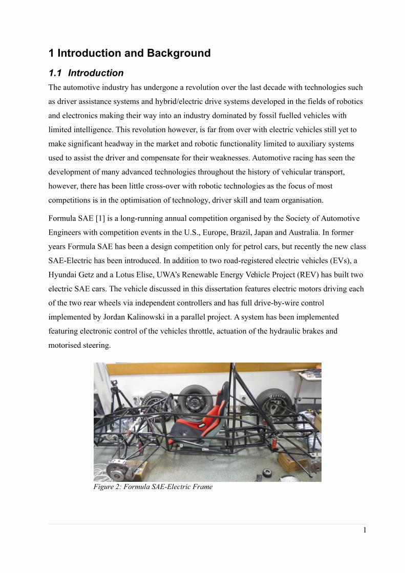
Formula SAE [1] is a long-running annual competition organised by the Society of Automotive

Engineers with competition events in the U.S., Europe, Brazil, Japan and Australia. In former

years Formula SAE has been a design competition only for petrol cars, but recently the new class

SAE-Electric has been introduced. In addition to two road-registered electric vehicles (EVs), a

Hyundai Getz and a Lotus Elise, UWA’s Renewable Energy Vehicle Project (REV) has built two

electric SAE cars. The vehicle discussed in this dissertation features electric motors driving each

of the two rear wheels via independent controllers and has full drive-by-wire control

implemented by Jordan Kalinowski in a parallel project. A system has been implemented

featuring electronic control of the vehicles throttle, actuation of the hydraulic brakes and

motorised steering.

Figure 2: Formula SAE-Electric Frame

1

This is outside the scope of the SAE competition which neither allows drive-by-wire nor

autonomous drive systems, however, the Autonomous SAE car project will provides UWA with a

platform for research into driverless cars. In particular, this project builds past research

conducted at UWA in which the REV group have implemented brake-by-wire and steer-by-wire

for a driver-assistance system on a BMW X5 [2]. The total automation and scope for

modification provided by the Autonomous SAE car give rise to research possibilities including,

but not limited to, automated performance driving, automated mapping and intelligent driving.

This dissertation describes the development of a map based autonomous driving system and

incorporates development of systems and technologies essential to any autonomous driving

application that may be developed in the future using this vehicle. Particular focus is given to the

hardware and software frameworks for implementation of this functionality, the integration of an

array of relevant sensors, LIDAR based road-edge detection and trajectory computation and

control. Safety systems have been considered as an integral part of the car's functionality and a

comprehensive range of controls have been developed in conjunction with Jordan Kalinowski.

1.2 Motivation

The development of the Autonomous SAE Car is primarily motivated by the great potential for

research into control systems, information processing algorithms and sensory techniques that are

made possible by creation of this vehicle as a research platform. This dissertation describes the

creation of such a platform, as well as a small proportion of the possible techniques that are able

to be developed and tested to further the field of mobile robotics. In particular, as the

Autonomous SAE Car is a race car by nature, research is possible within the rather

underdeveloped field of autonomous performance driving. Traditional automobile racing is

considered to be at the forefront of technology and has seen significant technological advances

which have filtered down to more mundane transportation systems and it is therefore expected

that the same will apply in the field of autonomous driving.

Research into autonomous driving has significant commercial potential as it represents the next

revolution in the efficiency of almost all transportation systems. Autonomous trains are already

fairly commonplace, particularly in niche operations such as mass rapid transport systems [3]

and mining [4] and have obvious advantages in terms of their operating costs and scheduling.

Automated truck convoying has also received significant commercial interest for similar reasons

[5]. It is therefore evident that technologies developed at UWA utilising the Autonomous SAE

Car have significant potential for real-world application in the near future.

2

2 Literature Review

Research into autonomous vehicles began in the 1980s with projects such as the EUREKA

Prometheus Project in Europe and the United States' Autonomous Land Vehicle Project [6]. The

DARPA Grand Challenges [7][8] in 2004 and 2005 saw teams of autonomous vehicles

competing to navigate a desert environment whilst the 2007 Urban Challenge [9][10][11]

required navigation of a road based course and adherence to traffic protocols. In Europe, the

VisLab Intercontinental Autonomous Challenge in 2010 [12] required an autonomous drive

following a leader car from Italy to China. These competitions saw massive development of the

field, with advanced technologies already becoming available for automotive use. Autonomous

driving technology is evolving rapidly and is well on its way to finding commercial use in years

to come. Google recently revealed that their fleet of autonomous cars had travelled 140,000

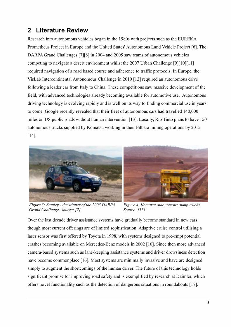
miles on US public roads without human intervention [13]. Locally, Rio Tinto plans to have 150

autonomous trucks supplied by Komatsu working in their Pilbara mining operations by 2015

[14].

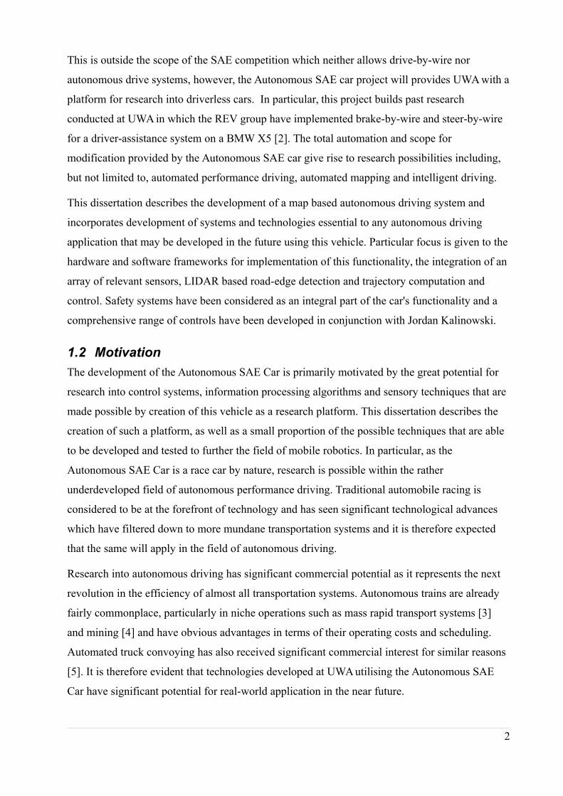
Figure 3: Stanley - the winner of the 2005 DARPA

Grand Challenge. Source: [7]

Figure 4: Komatsu autonomous dump trucks.

Source: [15]

Over the last decade driver assistance systems have gradually become standard in new cars

though most current offerings are of limited sophistication. Adaptive cruise control utilising a

laser sensor was first offered by Toyota in 1998, with systems designed to pre-empt potential

crashes becoming available on Mercedes-Benz models in 2002 [16]. Since then more advanced

camera-based systems such as lane-keeping assistance systems and driver drowsiness detection

have become commonplace [16]. Most systems are minimally invasive and have are designed

simply to augment the shortcomings of the human driver. The future of this technology holds

significant promise for improving road safety and is exemplified by research at Daimler, which

offers novel functionality such as the detection of dangerous situations in roundabouts [17].

3

Detailed research on control systems for autonomous driving have also been carried out at

Stanford [18] as well as at the University of Parma [19] and through a collaboration of Spanish

universities [20]. At UWA Lochlan Brown has conducted research into stability control using the

same car and has provided evidence that computer control of only the throttle has resulted in

significant advantages in increasing the vehicles stability [21]. A substantial body of work exists

concerning sensory techniques for use in autonomous vehicles including sensors such as GPS on

both road vehicles [22] and in agricultural applications [23] and LIDAR [24] [25] [26].

Recently technologies have matured and research into the potential of autonomous cars in racing

has begun, with projects such as Stanford University's autonomous Audi TTS, which has been

able to perform as well as seasoned racing drivers [27]. This project is of particular interest as its

aims in using electronic control systems to drive “at the limits” of the car's mechanical abilities

are similar to our project. A sophisticated suite of navigation sensors are used and have seen the

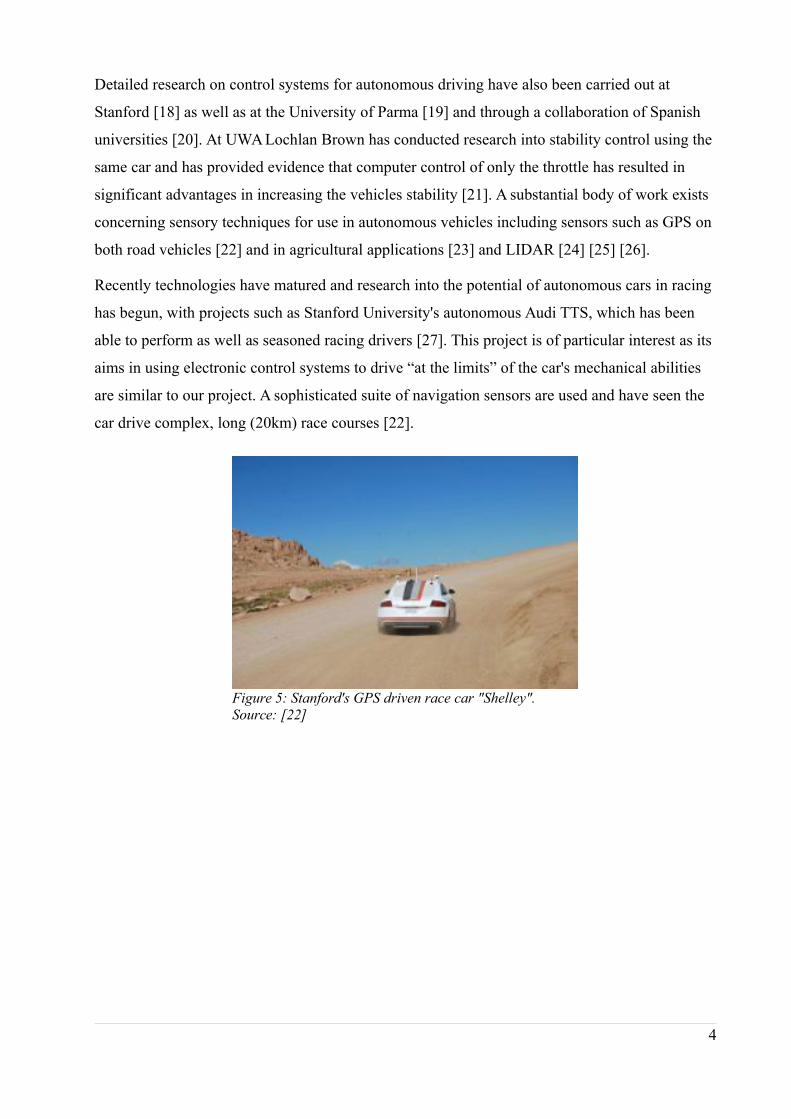
car drive complex, long (20km) race courses [22].

4

Figure 5: Stanford's GPS driven race car "Shelley".

Source: [22]

3 System Design

3.1 Overview and Requirements

The scope of the control system required for this project consists of everything from a

user-interface to physical actuation of the car's brake pedal and consists of a significant body of

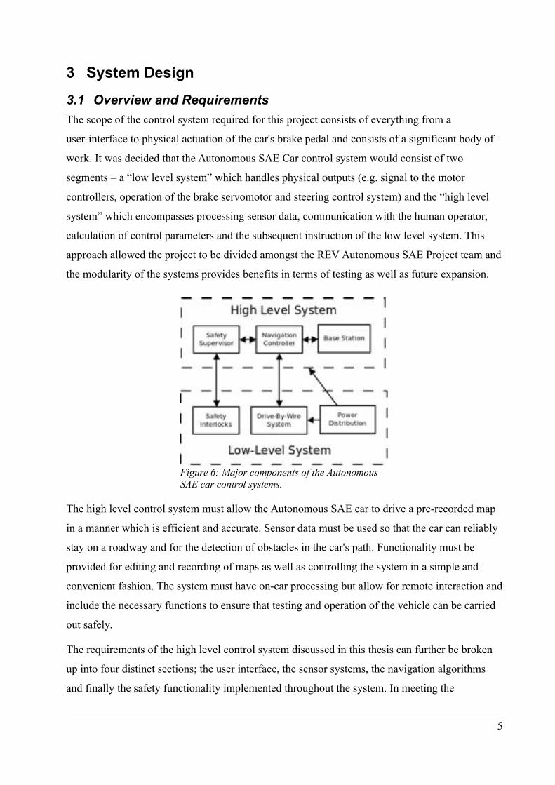
work. It was decided that the Autonomous SAE Car control system would consist of two

segments – a “low level system” which handles physical outputs (e.g. signal to the motor

controllers, operation of the brake servomotor and steering control system) and the “high level

system” which encompasses processing sensor data, communication with the human operator,

calculation of control parameters and the subsequent instruction of the low level system. This

approach allowed the project to be divided amongst the REV Autonomous SAE Project team and

the modularity of the systems provides benefits in terms of testing as well as future expansion.

Figure 6: Major components of the Autonomous

SAE car control systems.

The high level control system must allow the Autonomous SAE car to drive a pre-recorded map

in a manner which is efficient and accurate. Sensor data must be used so that the car can reliably

stay on a roadway and for the detection of obstacles in the car's path. Functionality must be

provided for editing and recording of maps as well as controlling the system in a simple and

convenient fashion. The system must have on-car processing but allow for remote interaction and

include the necessary functions to ensure that testing and operation of the vehicle can be carried

out safely.

The requirements of the high level control system discussed in this thesis can further be broken

up into four distinct sections; the user interface, the sensor systems, the navigation algorithms

and finally the safety functionality implemented throughout the system. In meeting the

5

requirements of these aspects of the project, a framework of hardware and software was created

as the basis for implementing functionality. This framework must thus be able to handle a

significant amount of data processing, interface with a variety of sensors, provide means for

interconnection with subsystems and also provide sufficient scope for expansion in future

projects.

3.2 Hardware Framework

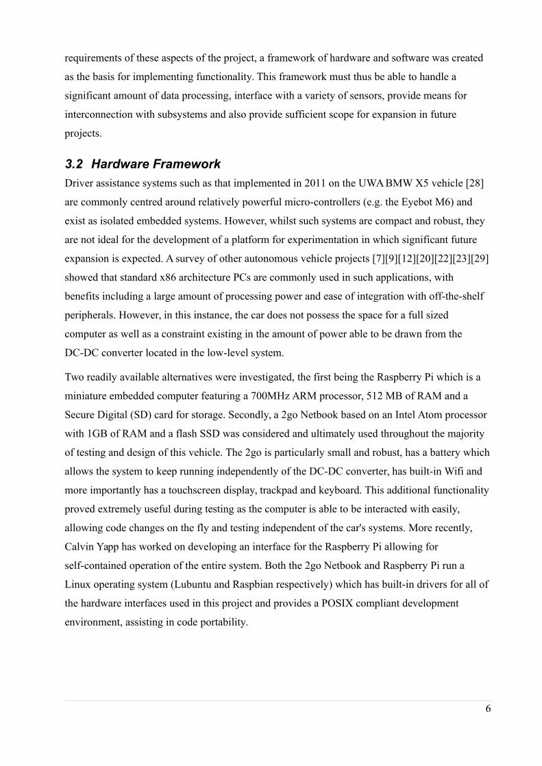
Driver assistance systems such as that implemented in 2011 on the UWA BMW X5 vehicle [28]

are commonly centred around relatively powerful micro-controllers (e.g. the Eyebot M6) and

exist as isolated embedded systems. However, whilst such systems are compact and robust, they

are not ideal for the development of a platform for experimentation in which significant future

expansion is expected. A survey of other autonomous vehicle projects [7][9][12][20][22][23][29]

showed that standard x86 architecture PCs are commonly used in such applications, with

benefits including a large amount of processing power and ease of integration with off-the-shelf

peripherals. However, in this instance, the car does not possess the space for a full sized

computer as well as a constraint existing in the amount of power able to be drawn from the

DC-DC converter located in the low-level system.

Two readily available alternatives were investigated, the first being the Raspberry Pi which is a

miniature embedded computer featuring a 700MHz ARM processor, 512 MB of RAM and a

Secure Digital (SD) card for storage. Secondly, a 2go Netbook based on an Intel Atom processor

with 1GB of RAM and a flash SSD was considered and ultimately used throughout the majority

of testing and design of this vehicle. The 2go is particularly small and robust, has a battery which

allows the system to keep running independently of the DC-DC converter, has built-in Wifi and

more importantly has a touchscreen display, trackpad and keyboard. This additional functionality

proved extremely useful during testing as the computer is able to be interacted with easily,

allowing code changes on the fly and testing independent of the car's systems. More recently,

Calvin Yapp has worked on developing an interface for the Raspberry Pi allowing for

self-contained operation of the entire system. Both the 2go Netbook and Raspberry Pi run a

Linux operating system (Lubuntu and Raspbian respectively) which has built-in drivers for all of

the hardware interfaces used in this project and provides a POSIX compliant development

environment, assisting in code portability.

6

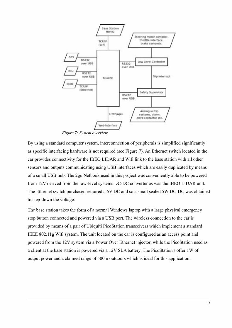
Figure 7: System overview

By using a standard computer system, interconnection of peripherals is simplified significantly

as specific interfacing hardware is not required (see Figure 7). An Ethernet switch located in the

car provides connectivity for the IBEO LIDAR and Wifi link to the base station with all other

sensors and outputs communicating using USB interfaces which are easily duplicated by means

of a small USB hub. The 2go Netbook used in this project was conveniently able to be powered

from 12V derived from the low-level systems DC-DC converter as was the IBEO LIDAR unit.

The Ethernet switch purchased required a 5V DC and so a small sealed 5W DC-DC was obtained

to step-down the voltage.

The base station takes the form of a normal Windows laptop with a large physical emergency

stop button connected and powered via a USB port. The wireless connection to the car is

provided by means of a pair of Ubiquiti PicoStation transceivers which implement a standard

IEEE 802.11g Wifi system. The unit located on the car is configured as an access point and

powered from the 12V system via a Power Over Ethernet injector, while the PicoStation used as

a client at the base station is powered via a 12V SLA battery. The PicoStation's offer 1W of

output power and a claimed range of 500m outdoors which is ideal for this application.

7

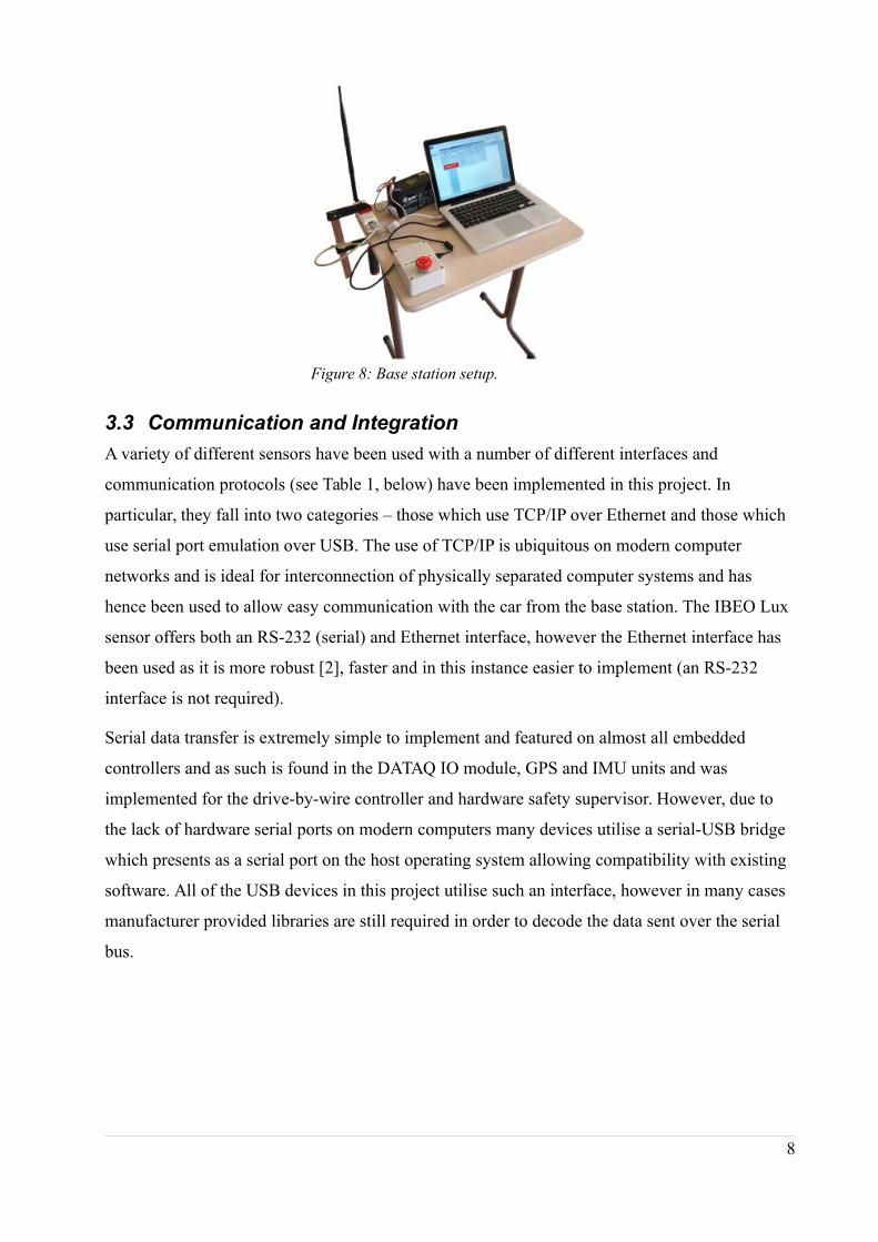
Figure 8: Base station setup.

3.3 Communication and Integration

A variety of different sensors have been used with a number of different interfaces and

communication protocols (see Table 1, below) have been implemented in this project. In

particular, they fall into two categories – those which use TCP/IP over Ethernet and those which

use serial port emulation over USB. The use of TCP/IP is ubiquitous on modern computer

networks and is ideal for interconnection of physically separated computer systems and has

hence been used to allow easy communication with the car from the base station. The IBEO Lux

sensor offers both an RS-232 (serial) and Ethernet interface, however the Ethernet interface has

been used as it is more robust [2], faster and in this instance easier to implement (an RS-232

interface is not required).

Serial data transfer is extremely simple to implement and featured on almost all embedded

controllers and as such is found in the DATAQ IO module, GPS and IMU units and was

implemented for the drive-by-wire controller and hardware safety supervisor. However, due to

the lack of hardware serial ports on modern computers many devices utilise a serial-USB bridge

which presents as a serial port on the host operating system allowing compatibility with existing

software. All of the USB devices in this project utilise such an interface, however in many cases

manufacturer provided libraries are still required in order to decode the data sent over the serial

bus.

8

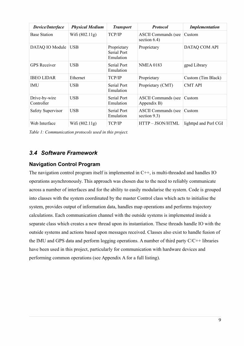
Device/Interface Physical Medium Transport Protocol Implementation

Base Station Wifi (802.11g) TCP/IP ASCII Commands (seesection 6.4)

Custom

DATAQ IO Module USB Proprietary Serial Port Emulation

Proprietary DATAQ COM API

GPS Receiver USB Serial Port Emulation

NMEA 0183 gpsd Library

IBEO LIDAR Ethernet TCP/IP Proprietary Custom (Tim Black)

IMU USB Serial Port Emulation

Proprietary (CMT) CMT API

Drive-by-wire Controller

USB Serial Port Emulation

ASCII Commands (see Appendix B)

Custom

Safety Supervisor USB Serial Port Emulation

ASCII Commands (seesection 9.3)

Custom

Web Interface Wifi (802.11g) TCP/IP HTTP – JSON/HTML lighttpd and Perl CGI

Table 1: Communication protocols used in this project.

3.4 Software Framework

Navigation Control Program

The navigation control program itself is implemented in C++, is multi-threaded and handles IO

operations asynchronously. This approach was chosen due to the need to reliably communicate

across a number of interfaces and for the ability to easily modularise the system. Code is grouped

into classes with the system coordinated by the master Control class which acts to initialise the

system, provides output of information data, handles map operations and performs trajectory

calculations. Each communication channel with the outside systems is implemented inside a

separate class which creates a new thread upon its instantiation. These threads handle IO with the

outside systems and actions based upon messages received. Classes also exist to handle fusion of

the IMU and GPS data and perform logging operations. A number of third party C/C++ libraries

have been used in this project, particularly for communication with hardware devices and

performing common operations (see Appendix A for a full listing).

9

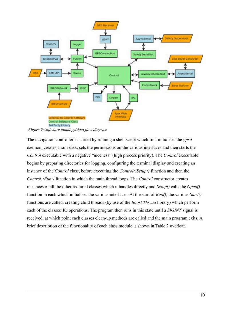
Figure 9: Software topology/data flow diagram

The navigation controller is started by running a shell script which first initialises the gpsd

daemon, creates a ram-disk, sets the permissions on the various interfaces and then starts the

Control executable with a negative “niceness” (high process priority). The Control executable

begins by preparing directories for logging, configuring the terminal display and creating an

instance of the Control class, before executing the Control::Setup() function and then the

Control::Run() function in which the main thread loops. The Control constructor creates

instances of all the other required classes which it handles directly and Setup() calls the Open()

function in each which initialises the various interfaces. At the start of Run(), the various Start()

functions are called, creating child threads (by use of the Boost.Thread library) which perform

each of the classes' IO operations. The program then runs in this state until a SIGINT signal is

received, at which point each classes clean-up methods are called and the main program exits. A

brief description of the functionality of each class module is shown in Table 2 overleaf.

10

IO Classes

Name Description

CarNetwork The CarNetwork class utilises the Berekely sockets API to provide a server for communication with the base station. Messages received are parsed and appropriate functions called to deal with their results.

GPSConnection GPSConnection uses libgpsmm which is part of the gpsd suite to communicate with the gpsd daemon which receives messages from the GPS receiver. The received data is parsed and calls are made to Fusion member functions to act upon the new position/velocity/heading information.

IBEO The IBEO class contains Tim Black's [2] implementation of the IBEO Ethernet protocol which decodes the byte stream received via IBEONetwork as well as codedeveloped for the Autonomous SAE car which handles processing and acting upon the received data. The received object data is used to project detected obstacles (“fenceposts”) back onto the map current loaded in memory and the scan data is used to for detection of the road edges (see section 4.3). Two sets of files are written out for every 200ms containing the received scan/object data for review and the most recent data is written to the ram-disk for display in the web interface.

IBEONetwork IBEONetwork was implemented in this project and uses the Berkeley sockets API to connect to the IBEO scanner.

IPC The IPC (inter-process communication) class creates and listens to a named pipe for commands sent from an interface to the Control program. When each new line terminated command (and comma separated arguments) is received, it is parsed and appropriate action taken.

LowLevelSerialOut This class uses the AsyncSerial library (a wrapper for the Boost.asio library) to communicate with the drive-by-wire controller over a serial port. A constant streamof commands (see Appendix B) are transmitted based on the current set points and received data including command acknowledgement, error codes and informational messages are parsed and acted upon as appropriate.

SafetySerialOut This class is similar to the above except that it interacts with the hardware safety supervisor module (see section 6.3).

Xsens The Xsens class uses the vendor-provided CMT API to receive data from the IMU.The data is then processed to provide acceleration and heading data in the correct format for use in the Fusion class.

Utility Classes

Name Description

Control The Control class's main loop handles output of information to the terminal displayand to a log file located on the ram-disk for use by the web interface. This class also contains the functions used to generate the trajectory for autonomous driving, functions that deal with mapping functionality as well as (static) utility functions which are used in various parts of the program.

Fusion The Fusion class contains a set of functions which are called when new GPS data arrives and are used to fuse GPS and IMU data in order to produce improved heading and position estimates. This class performs extensive logging of the data itproduces and performs a set of actions each time a new estimate is generated.

Logger The Logger class is used extensively throughout the program for file IO operations. It allows recording of time-stamped data as well as the writing of lock files to indicate when a log is currently being written out.

Table 2: Description of Control program modules.

11

Base Station Hardware IO Software

The base station software provides three primary features – interfacing with the USB emergency

stop button, generating the heartbeat signal and relaying these signals to the navigation controller

via a TCP/IP connection over Wifi. The software generates a binary valued heartbeat signal,

outputs it to a DATAQ DI-148 USB IO interface and reads two input lines – one which is used to

detect the position of the emergency stop button via its NO contacts and another which receives

the heartbeat signal via the stop button's NC contacts. The state of the heartbeat read by the

DI-148 is then used for transmission to the car. This arrangement allows for instant detection of

the buttons position as well as providing a fail-safe verification that the interface is working via

the heartbeat signal. In the case that the stop button is pressed, the base station will send an

emergency stop command as well as the heartbeat being interrupted (see Appendix C for the

wiring diagram).

The ability to control the car using a USB hand controller was also implemented as a secondary

feature which was utilised during integration testing of the drive-by-wire system. Two axes of

controller are read as well as two buttons (alarm and emergency stop) and sent to the navigation

controller via the network link which are then sent to the drive-by-wire controller if the

navigation controller is in manual mode. Additionally, buttons are provided in the UI for sending

commands to the navigation controller for changing safety profile (see section 6.1), enabling

manual mode and emergency stopping the car.

The base station software was implemented in Microsoft C#.NET as a COM/ActiveX control

which provides an API for communication with the DATAQ DI-148 was readily available. In

addition, the availability of SharpDX, a DirectX API made interfacing with the USB controller

via DirectInput relatively simple. The base station UI is a Windows Forms Application and as

such is event driven, with events generated by interaction with the form itself, by timers or by the

DATAQ ActiveX control. The TCP/IP connection with the navigation controller is established

using the .NET Socket library and works synchronously, blocking execution until the

acknowledgement of each command is received after sending (or a time-out occurs). The

command set implemented in the base station software and the navigation controller's

CarNetwork class are shown below in Table 3.

12

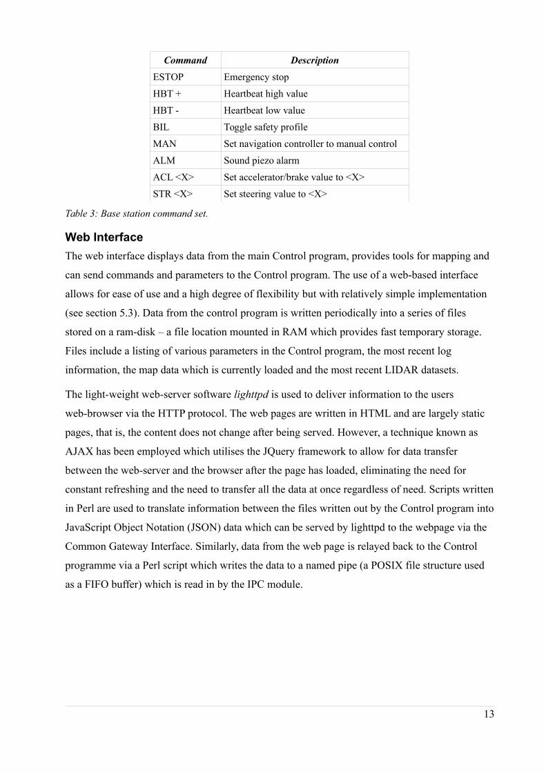
Command Description

ESTOP Emergency stop

HBT + Heartbeat high value

HBT - Heartbeat low value

BIL Toggle safety profile

MAN Set navigation controller to manual control

ALM Sound piezo alarm

ACL <X> Set accelerator/brake value to <X>

STR <X> Set steering value to <X>

Table 3: Base station command set.

Web Interface

The web interface displays data from the main Control program, provides tools for mapping and

can send commands and parameters to the Control program. The use of a web-based interface

allows for ease of use and a high degree of flexibility but with relatively simple implementation

(see section 5.3). Data from the control program is written periodically into a series of files

stored on a ram-disk – a file location mounted in RAM which provides fast temporary storage.

Files include a listing of various parameters in the Control program, the most recent log

information, the map data which is currently loaded and the most recent LIDAR datasets.

The light-weight web-server software lighttpd is used to deliver information to the users

web-browser via the HTTP protocol. The web pages are written in HTML and are largely static

pages, that is, the content does not change after being served. However, a technique known as

AJAX has been employed which utilises the JQuery framework to allow for data transfer

between the web-server and the browser after the page has loaded, eliminating the need for

constant refreshing and the need to transfer all the data at once regardless of need. Scripts written

in Perl are used to translate information between the files written out by the Control program into

JavaScript Object Notation (JSON) data which can be served by lighttpd to the webpage via the

Common Gateway Interface. Similarly, data from the web page is relayed back to the Control

programme via a Perl script which writes the data to a named pipe (a POSIX file structure used

as a FIFO buffer) which is read in by the IPC module.

13

4 Sensor Selection and Integration

4.1 Overview

An autonomous vehicle requires an array of sensors which are able to supply data regarding its

current position and kinematics as well as knowledge of the environment surrounding it.

Reliability, accuracy and sensor coverage are highly important as the information used for

navigation is critical to the safe operation of the vehicle and typically an array of sensors is

implemented with redundancy and extended capabilities obtained through multi-sensor data

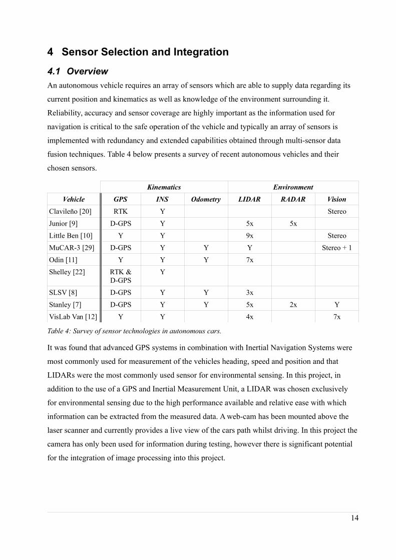
fusion techniques. Table 4 below presents a survey of recent autonomous vehicles and their

chosen sensors.

Kinematics Environment

Vehicle GPS INS Odometry LIDAR RADAR Vision

Clavileño [20] RTK Y Stereo

Junior [9] D-GPS Y 5x 5x

Little Ben [10] Y Y 9x Stereo

MuCAR-3 [29] D-GPS Y Y Y Stereo + 1

Odin [11] Y Y Y 7x

Shelley [22] RTK &D-GPS

Y

SLSV [8] D-GPS Y Y 3x

Stanley [7] D-GPS Y Y 5x 2x Y

VisLab Van [12] Y Y 4x 7x

Table 4: Survey of sensor technologies in autonomous cars.

It was found that advanced GPS systems in combination with Inertial Navigation Systems were

most commonly used for measurement of the vehicles heading, speed and position and that

LIDARs were the most commonly used sensor for environmental sensing. In this project, in

addition to the use of a GPS and Inertial Measurement Unit, a LIDAR was chosen exclusively

for environmental sensing due to the high performance available and relative ease with which

information can be extracted from the measured data. A web-cam has been mounted above the

laser scanner and currently provides a live view of the cars path whilst driving. In this project the

camera has only been used for information during testing, however there is significant potential

for the integration of image processing into this project.

14

4.2 Position and Orientation

Global Positioning System

Standard GPS receivers compute their position by measurement of the time differences in

receiving “pseudo-range” signals from at least four GPS satellites [30]. Through knowledge of

the satellite’s orbital parameters this information is used to calculate a position on the Earth’s

surface. Typically, velocity information calculated by means of the Doppler Effect is also

available. When a changing position is detected the GPS module will also report a calculated

“track angle”, that is, a bearing in the direction of motion.

The accuracy of standard GPS devices has improved over recent years with the cessation of

“Selective Ability”, upgrades to the satellite constellation and the introduction of more advanced

measurement and augmentation systems [30]. Differential GPS utilises ground based stations to

broadcast GPS error corrections for localised areas and Satellite Based Augmentation Systems

such as the US Wide Area Augmentation System perform a similar function using additional

geostationary satellites. Real-Time Kinematic systems utilise a local ground station and

determine the relative position between the moving object and the ground station via

measurement of the GPS carrier phase – such systems are able to achieve centimetre level

accuracy [31].

A variety of commercial products are available which provide built-in sensor fusion as well as

functionality including D-GPS correction and RTK measurements. The cost is proportional to the

accuracy and ranges from around $1000 for sub-meter accuracy (e.g. D-GPS), to around $5000

for decimetre accuracy (dual channel commercial SBAS) to tens of thousands for advanced

survey-grade RTK systems [31]. Products such as the Applanix POS LV which include these

high-level features have commonly been used in autonomous vehicles [22][32], however, with

no public SBAS available in Australia and systems such as D-GPS and RTK still extremely

expensive, a standard GPS device was selected for this project.

The module used in this project is a QStarz BT-Q818X – it possesses a USB interface and sends

NMEA 0183 GPS data via a virtual serial port. The GPS unit includes a Li-Ion battery, which

allows it to operate continuously independent of the car’s power system. The unit is configurable

via a PC application and in this project has been configured to send GPSRMC messages at a rate

of 5Hz.

15

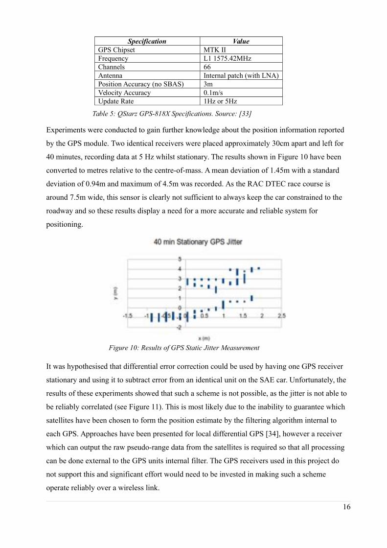
Specification Value

GPS Chipset MTK IIFrequency L1 1575.42MHzChannels 66Antenna Internal patch (with LNA)Position Accuracy (no SBAS) 3mVelocity Accuracy 0.1m/sUpdate Rate 1Hz or 5Hz

Table 5: QStarz GPS-818X Specifications. Source: [33]

Experiments were conducted to gain further knowledge about the position information reported

by the GPS module. Two identical receivers were placed approximately 30cm apart and left for

40 minutes, recording data at 5 Hz whilst stationary. The results shown in Figure 10 have been

converted to metres relative to the centre-of-mass. A mean deviation of 1.45m with a standard

deviation of 0.94m and maximum of 4.5m was recorded. As the RAC DTEC race course is

around 7.5m wide, this sensor is clearly not sufficient to always keep the car constrained to the

roadway and so these results display a need for a more accurate and reliable system for

positioning.

Figure 10: Results of GPS Static Jitter Measurement

It was hypothesised that differential error correction could be used by having one GPS receiver

stationary and using it to subtract error from an identical unit on the SAE car. Unfortunately, the

results of these experiments showed that such a scheme is not possible, as the jitter is not able to

be reliably correlated (see Figure 11). This is most likely due to the inability to guarantee which

satellites have been chosen to form the position estimate by the filtering algorithm internal to

each GPS. Approaches have been presented for local differential GPS [34], however a receiver

which can output the raw pseudo-range data from the satellites is required so that all processing

can be done external to the GPS units internal filter. The GPS receivers used in this project do

not support this and significant effort would need to be invested in making such a scheme

operate reliably over a wireless link.

16

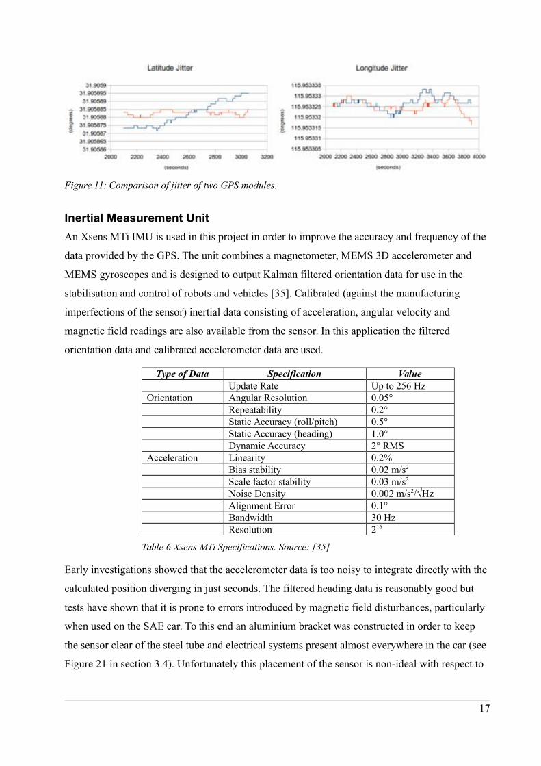
Figure 11: Comparison of jitter of two GPS modules.

Inertial Measurement Unit

An Xsens MTi IMU is used in this project in order to improve the accuracy and frequency of the

data provided by the GPS. The unit combines a magnetometer, MEMS 3D accelerometer and

MEMS gyroscopes and is designed to output Kalman filtered orientation data for use in the

stabilisation and control of robots and vehicles [35]. Calibrated (against the manufacturing

imperfections of the sensor) inertial data consisting of acceleration, angular velocity and

magnetic field readings are also available from the sensor. In this application the filtered

orientation data and calibrated accelerometer data are used.

Type of Data Specification Value

Update Rate Up to 256 HzOrientation Angular Resolution 0.05°

Repeatability 0.2°Static Accuracy (roll/pitch) 0.5°Static Accuracy (heading) 1.0°Dynamic Accuracy 2° RMS

Acceleration Linearity 0.2%Bias stability 0.02 m/s2

Scale factor stability 0.03 m/s2

Noise Density 0.002 m/s2/√HzAlignment Error 0.1°Bandwidth 30 HzResolution 216

Table 6 Xsens MTi Specifications. Source: [35]

Early investigations showed that the accelerometer data is too noisy to integrate directly with the

calculated position diverging in just seconds. The filtered heading data is reasonably good but

tests have shown that it is prone to errors introduced by magnetic field disturbances, particularly

when used on the SAE car. To this end an aluminium bracket was constructed in order to keep

the sensor clear of the steel tube and electrical systems present almost everywhere in the car (see

Figure 21 in section 3.4). Unfortunately this placement of the sensor is non-ideal with respect to

17

collecting inertial data (ideally the sensor would be placed in a stable position near the centre of

mass), however, the configuration has proven delivered far better heading measurements.

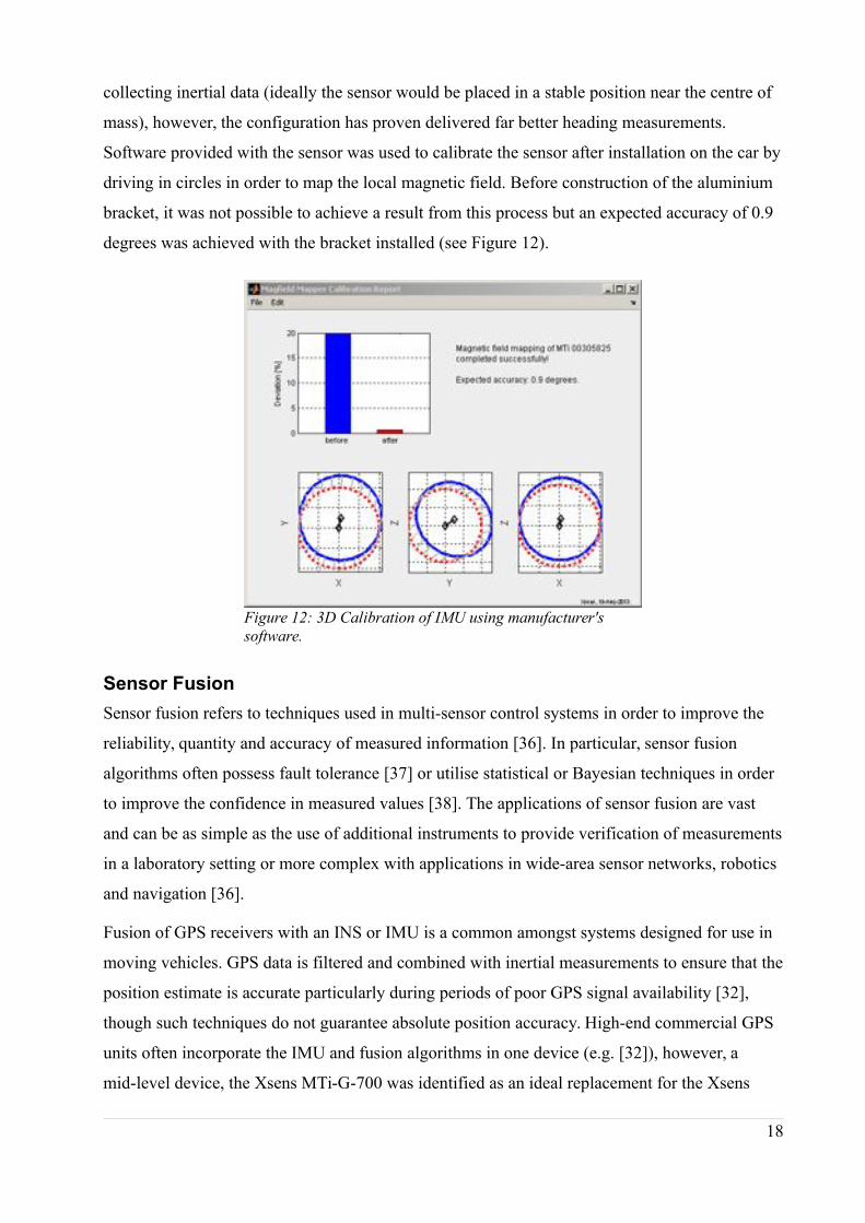
Software provided with the sensor was used to calibrate the sensor after installation on the car by

driving in circles in order to map the local magnetic field. Before construction of the aluminium

bracket, it was not possible to achieve a result from this process but an expected accuracy of 0.9

degrees was achieved with the bracket installed (see Figure 12).

Figure 12: 3D Calibration of IMU using manufacturer's

software.

Sensor Fusion

Sensor fusion refers to techniques used in multi-sensor control systems in order to improve the

reliability, quantity and accuracy of measured information [36]. In particular, sensor fusion

algorithms often possess fault tolerance [37] or utilise statistical or Bayesian techniques in order

to improve the confidence in measured values [38]. The applications of sensor fusion are vast

and can be as simple as the use of additional instruments to provide verification of measurements

in a laboratory setting or more complex with applications in wide-area sensor networks, robotics

and navigation [36].

Fusion of GPS receivers with an INS or IMU is a common amongst systems designed for use in

moving vehicles. GPS data is filtered and combined with inertial measurements to ensure that the

position estimate is accurate particularly during periods of poor GPS signal availability [32],

though such techniques do not guarantee absolute position accuracy. High-end commercial GPS

units often incorporate the IMU and fusion algorithms in one device (e.g. [32]), however, a

mid-level device, the Xsens MTi-G-700 was identified as an ideal replacement for the Xsens

18

MTi and QStarz GPS receiver used in this project. The MTi-G combines an Xsens IMU with a

good quality GPS receiver featuring an external antenna and incorporates a proprietary sensor

fusion algorithm which can create position, velocity and orientation estimates at up to 400 Hz

[39]. Unfortunately, it was not possible to obtain the device for inclusion in the project and so

sensor fusion techniques were investigated at the navigation controller level.

Vehicle Heading

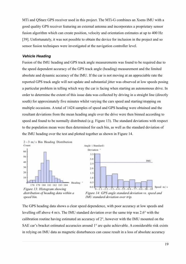
Fusion of the IMU heading and GPS track angle measurements was found to be required due to

the speed dependent accuracy of the GPS track angle (heading) measurement and the limited

absolute and dynamic accuracy of the IMU. If the car is not moving at an appreciable rate the

reported GPS track angle will not update and substantial jitter was observed at low speeds posing

a particular problem in telling which way the car is facing when starting an autonomous drive. In

order to determine the extent of this issue data was collected by driving in a straight line (directly

south) for approximately five minutes whilst varying the cars speed and starting/stopping on

multiple occasions. A total of 1424 samples of speed and GPS heading were obtained and the

resultant deviations from the mean heading angle over the drive were then binned according to

speed and found to be normally distributed (e.g. Figure 13). The standard deviations with respect

to the population mean were then determined for each bin, as well as the standard deviation of

the IMU heading over the test and plotted together as shown in Figure 14.

Figure 13: Histogram showing

distribution of heading data within a

speed bin.

Figure 14: GPS angle standard deviation vs. speed and

IMU standard deviation over trip.

The GPS heading data shows a clear speed dependence, with poor accuracy at low speeds and

levelling off above 4 m/s. The IMU standard deviation over the same trip was 2.6° with the

calibration routine having estimated an accuracy of 2°, however with the IMU mounted on the

SAE car’s bracket estimated accuracies around 1° are quite achievable. A considerable risk exists

in relying on IMU data as magnetic disturbances can cause result in a loss of absolute accuracy

19

IMU

and a “wandering” heading and though the aluminium bracket appears to have prevented this

occurring on the SAE car, the phenomenon was observed several times during testing.

A speed-dependent weighted average with characteristics based on these observations was

therefore implemented in order to ensure that the most accurate heading at all speeds. Such an

approach is based upon the algorithm presented by Elmenreich [38] but with a variable rather

than static weighting. The fundamental premise of sensor fusion is to improve the accuracy of a

measurement by means of combination of data from multiple sensors and in this case we seek to

minimise the variance of the measured vehicle heading. By deriving weightings for the

measurements of each sensor, we can create a measurement with lower variance than that of the

sensors taken individually. Treating the GPS and IMU as random variables XG and XI

respectively we can model the fused measurement as a Gaussian random variable where

Z=wG X G+wI X I .

Then, applying the method of Elmenreich [38] to this specific case we can first use the fact the

variables are independently Gaussian distributed to give the combined variance:

σ Z

2=wG

2 σ G

2 +wI

2σ I

2

Since Z is a weighted average and we require E [Z ]=E [X ] :

wG+w

I=1

We then seek to extremise σZ

2 by setting both partial derivatives to zero:

∂σ Z2

∂ wG

= ∂∂ wG

[ wG

2 σ G

2 +(1−wG)2σ I

2 ]=2w Gσ G

2 −2(1−wG)σ I

2=0

∂σ Z

2

∂ wI

=2w I σ I

2−2(1−wI )σ G

2 =0

Checking the second derivatives it is clear that:

∂2σ Z2

∂w I

2=2σ I

2+2σ G

2 > 0 ∧∂2 σ Z

2

∂ wG

2> 0

Giving:

wG=1

1+σ G

2

σ I

2

, wI=1

1+σ I

2

σ G

2

⇒ σ Z

2 =1

1

σ G

2+

1

σ I

2

20

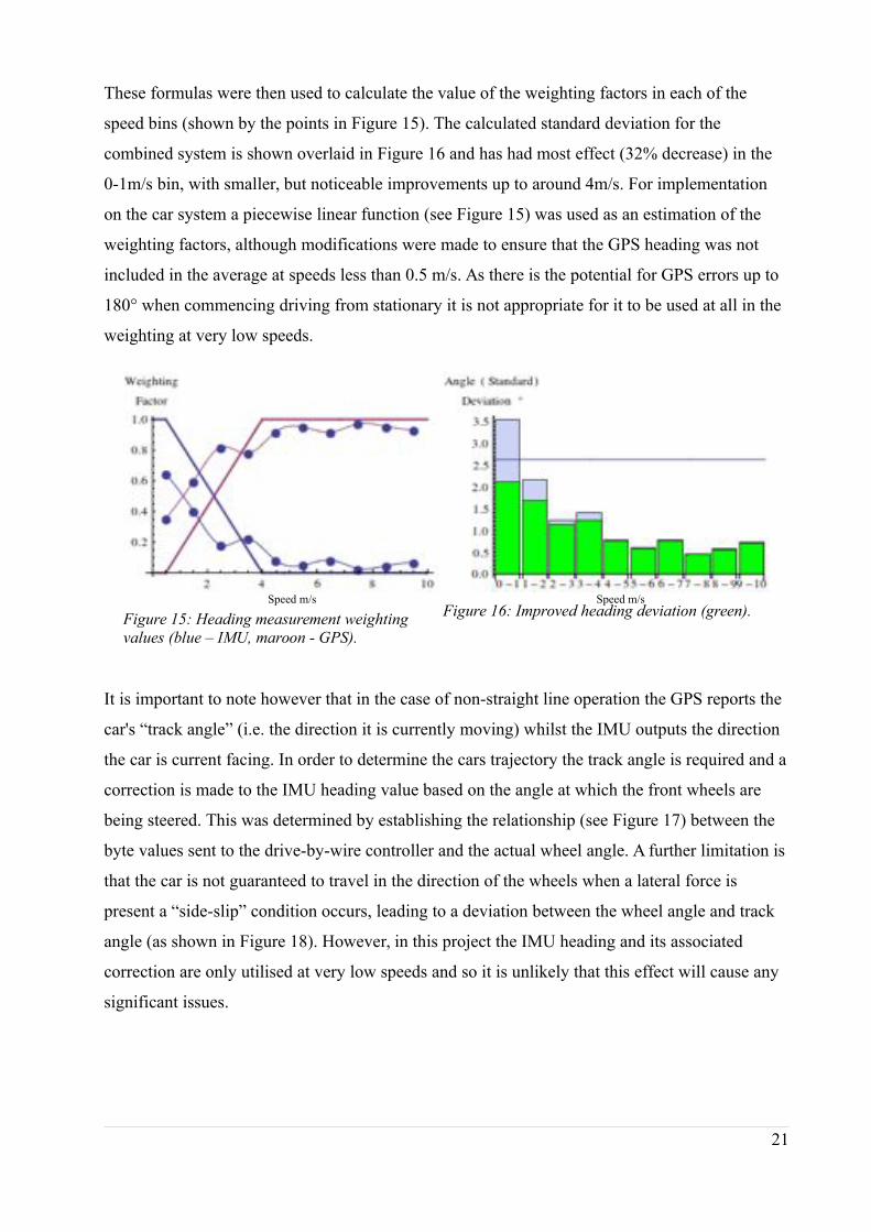
These formulas were then used to calculate the value of the weighting factors in each of the

speed bins (shown by the points in Figure 15). The calculated standard deviation for the

combined system is shown overlaid in Figure 16 and has had most effect (32% decrease) in the

0-1m/s bin, with smaller, but noticeable improvements up to around 4m/s. For implementation

on the car system a piecewise linear function (see Figure 15) was used as an estimation of the

weighting factors, although modifications were made to ensure that the GPS heading was not

included in the average at speeds less than 0.5 m/s. As there is the potential for GPS errors up to

180° when commencing driving from stationary it is not appropriate for it to be used at all in the

weighting at very low speeds.

Figure 15: Heading measurement weighting

values (blue – IMU, maroon - GPS).

Figure 16: Improved heading deviation (green).

It is important to note however that in the case of non-straight line operation the GPS reports the

car's “track angle” (i.e. the direction it is currently moving) whilst the IMU outputs the direction

the car is current facing. In order to determine the cars trajectory the track angle is required and a

correction is made to the IMU heading value based on the angle at which the front wheels are

being steered. This was determined by establishing the relationship (see Figure 17) between the

byte values sent to the drive-by-wire controller and the actual wheel angle. A further limitation is

that the car is not guaranteed to travel in the direction of the wheels when a lateral force is

present a “side-slip” condition occurs, leading to a deviation between the wheel angle and track

angle (as shown in Figure 18). However, in this project the IMU heading and its associated

correction are only utilised at very low speeds and so it is unlikely that this effect will cause any

significant issues.

21

Speed m/s Speed m/s

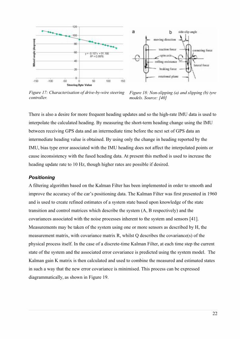
Figure 17: Characterisation of drive-by-wire steering

controller.

Figure 18: Non-slipping (a) and slipping (b) tyre

models. Source: [40]

There is also a desire for more frequent heading updates and so the high-rate IMU data is used to

interpolate the calculated heading. By measuring the short-term heading change using the IMU

between receiving GPS data and an intermediate time before the next set of GPS data an

intermediate heading value is obtained. By using only the change in heading reported by the

IMU, bias type error associated with the IMU heading does not affect the interpolated points or

cause inconsistency with the fused heading data. At present this method is used to increase the

heading update rate to 10 Hz, though higher rates are possible if desired.

Positioning

A filtering algorithm based on the Kalman Filter has been implemented in order to smooth and

improve the accuracy of the car’s positioning data. The Kalman Filter was first presented in 1960

and is used to create refined estimates of a system state based upon knowledge of the state

transition and control matrices which describe the system (A, B respectively) and the

covariances associated with the noise processes inherent to the system and sensors [41].

Measurements may be taken of the system using one or more sensors as described by H, the

measurement matrix, with covariance matrix R, whilst Q describes the covariance(s) of the

physical process itself. In the case of a discrete-time Kalman Filter, at each time step the current

state of the system and the associated error covariance is predicted using the system model. The

Kalman gain K matrix is then calculated and used to combine the measured and estimated states

in such a way that the new error covariance is minimised. This process can be expressed

diagrammatically, as shown in Figure 19.

22

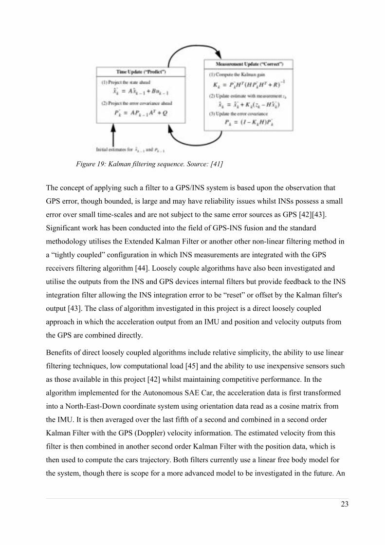
Figure 19: Kalman filtering sequence. Source: [41]

The concept of applying such a filter to a GPS/INS system is based upon the observation that

GPS error, though bounded, is large and may have reliability issues whilst INSs possess a small

error over small time-scales and are not subject to the same error sources as GPS [42][43].

Significant work has been conducted into the field of GPS-INS fusion and the standard

methodology utilises the Extended Kalman Filter or another other non-linear filtering method in

a “tightly coupled” configuration in which INS measurements are integrated with the GPS

receivers filtering algorithm [44]. Loosely couple algorithms have also been investigated and

utilise the outputs from the INS and GPS devices internal filters but provide feedback to the INS

integration filter allowing the INS integration error to be “reset” or offset by the Kalman filter's

output [43]. The class of algorithm investigated in this project is a direct loosely coupled

approach in which the acceleration output from an IMU and position and velocity outputs from

the GPS are combined directly.

Benefits of direct loosely coupled algorithms include relative simplicity, the ability to use linear

filtering techniques, low computational load [45] and the ability to use inexpensive sensors such

as those available in this project [42] whilst maintaining competitive performance. In the

algorithm implemented for the Autonomous SAE Car, the acceleration data is first transformed

into a North-East-Down coordinate system using orientation data read as a cosine matrix from

the IMU. It is then averaged over the last fifth of a second and combined in a second order

Kalman Filter with the GPS (Doppler) velocity information. The estimated velocity from this

filter is then combined in another second order Kalman Filter with the position data, which is

then used to compute the cars trajectory. Both filters currently use a linear free body model for

the system, though there is scope for a more advanced model to be investigated in the future. An

23

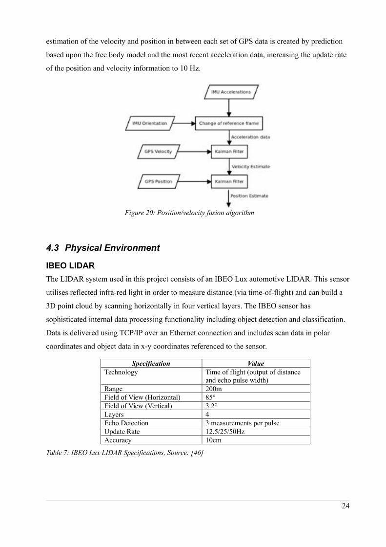
estimation of the velocity and position in between each set of GPS data is created by prediction

based upon the free body model and the most recent acceleration data, increasing the update rate

of the position and velocity information to 10 Hz.

Figure 20: Position/velocity fusion algorithm

4.3 Physical Environment

IBEO LIDAR

The LIDAR system used in this project consists of an IBEO Lux automotive LIDAR. This sensor

utilises reflected infra-red light in order to measure distance (via time-of-flight) and can build a

3D point cloud by scanning horizontally in four vertical layers. The IBEO sensor has

sophisticated internal data processing functionality including object detection and classification.

Data is delivered using TCP/IP over an Ethernet connection and includes scan data in polar

coordinates and object data in x-y coordinates referenced to the sensor.

Specification Value

Technology Time of flight (output of distance and echo pulse width)

Range 200mField of View (Horizontal) 85°Field of View (Vertical) 3.2°Layers 4Echo Detection 3 measurements per pulseUpdate Rate 12.5/25/50HzAccuracy 10cm

Table 7: IBEO Lux LIDAR Specifications, Source: [46]

24

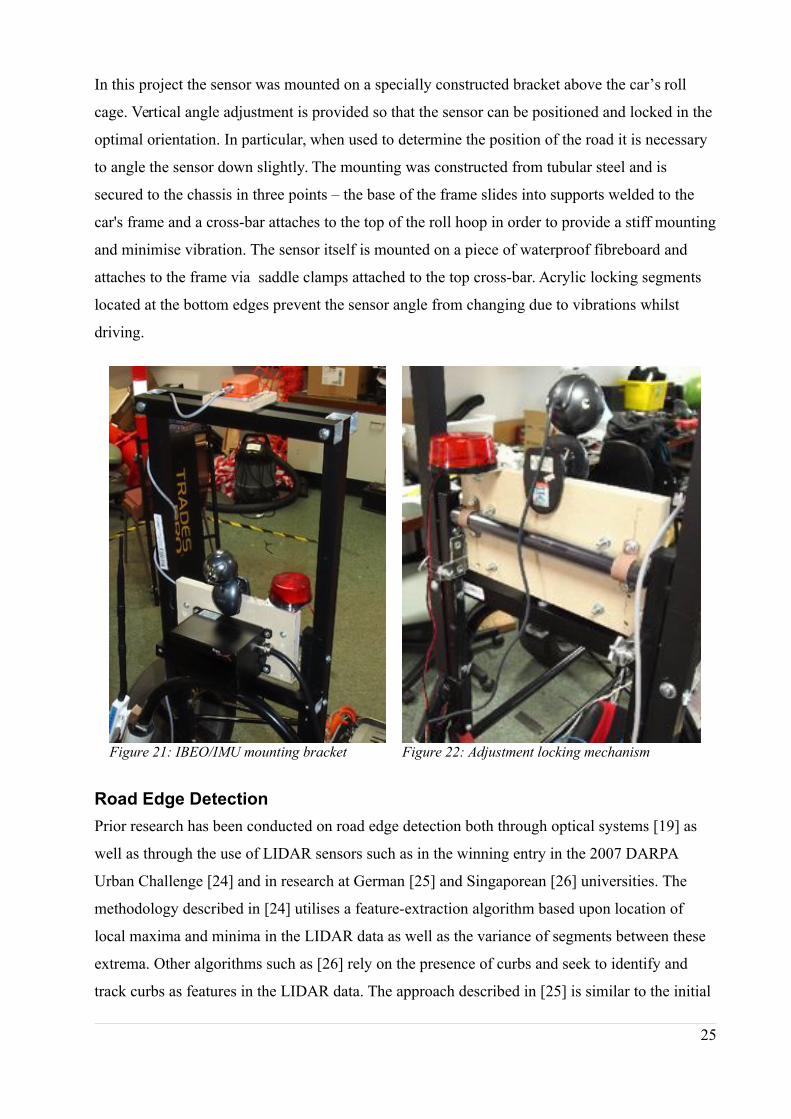
In this project the sensor was mounted on a specially constructed bracket above the car’s roll

cage. Vertical angle adjustment is provided so that the sensor can be positioned and locked in the

optimal orientation. In particular, when used to determine the position of the road it is necessary

to angle the sensor down slightly. The mounting was constructed from tubular steel and is

secured to the chassis in three points – the base of the frame slides into supports welded to the

car's frame and a cross-bar attaches to the top of the roll hoop in order to provide a stiff mounting

and minimise vibration. The sensor itself is mounted on a piece of waterproof fibreboard and

attaches to the frame via saddle clamps attached to the top cross-bar. Acrylic locking segments

located at the bottom edges prevent the sensor angle from changing due to vibrations whilst

driving.

Figure 21: IBEO/IMU mounting bracket Figure 22: Adjustment locking mechanism

Road Edge Detection

Prior research has been conducted on road edge detection both through optical systems [19] as

well as through the use of LIDAR sensors such as in the winning entry in the 2007 DARPA

Urban Challenge [24] and in research at German [25] and Singaporean [26] universities. The

methodology described in [24] utilises a feature-extraction algorithm based upon location of

local maxima and minima in the LIDAR data as well as the variance of segments between these

extrema. Other algorithms such as [26] rely on the presence of curbs and seek to identify and

track curbs as features in the LIDAR data. The approach described in [25] is similar to the initial

25

algorithm employed here and attempts to seek appropriate linear fits to the road surface, however

their estimates were then combined with filtered reflectivity data in order to find the road

surface. In both of the latter two cases a Kalman filter is used to track the position of the road

edges temporally.

In this project the IBEO sensor's “scan data” sets consisting of polar angle/radial distance pairs

were analysed in order to find the horizontal extent of the road surface. By mounting the sensor

at height (i.e. above the roll cage) the sensor plane intersects the road in such a way that radial

distance variations are recorded for both variations in the height of the road/curb as well as in the

distance in front of the car (see Figure 23). It was found during experimentation with the IBEO

sensor that observed that road points on a bitumen surface tend to be arranged collinearly with a

small deviation whereas points belonging to uneven surfaces (such as grass and curbs) tend to be

scattered, with their arrangement depending on the contour of the surface away from the road

edge.

Figure 23: LIDAR edge detection geometry.

In the case of the Autonomous SAE car, detection which relies upon the presence of curbs or

marked lines is not feasible as race tracks, unlike public roads may not have such features (in

particular, the RAC DTEC track has grass/dirt edges). In addition, the algorithm must be able to

dynamically detect road edges whilst the car is moving (and turning) and should have an

accuracy better than 0.5m at each side. The algorithm developed here therefore focuses on

identifying the presence of a road section rather than the presence of a particular edge

characteristic and will thus work both on curbed and non-curbed roads.

26

The following hypothesis was developed for the detection of road edges:

Roads should be: Mostly, but not always close to the centre of the scan

Smooth (e.g. points co-linear)

In the same plane as the car (e.g. small horizontal gradient)

Edges may be: Scattered (non-linear)

Sloped

Raised/lowered

An additional property, considered later, is that the road-edge boundary should be locatable in a

predictable fashion over time.

The algorithm implemented in this project operates by first identifying a candidate group of

points close to the centre of the scan data which meet the slope condition (i.e. the slope of a line

through these points is less than a pre-set value). This group is then expanded iteratively, with a

least-squares linear regression performed at each step. By minimising the square residuals

between the fit line (y) and the data (xi,yi), this technique obtains the most appropriate line for the

given data set, the success of which can be measured by means of the product-moment

correlation coefficient r. In this case, the slope (b) and r2 values are of relevance and are

tabulated.

Specifically; y=( y−b x)+b x , r=sxy

s x sy

where

b=sxy

s x2

, sxy=∑i=1

n

xi y i

n− x y , sx

2=∑i=1

n

xi

2

n− x

2, sx

2=∑i=1

n

y i

2

n− y

2

This technique is performed independently for the left and right hand sides of the candidate point

group to allow for the fact that roads are often sloped about the centre (e.g. to let water run off)

which results in improved accuracy. In the initial implementation, the road-edges were then

determined to be the outer edges of the candidate groups which maximised the respective

correlation coefficients and met the slope condition. In summary, the algorithm follows this

sequence:

1. Step out from the centre of the dataset looking for a point cluster which meets the slope

condition. Interleave looking to the left and right.

2. Perform stepping to the left and right (seperately) of this cluster , increasing the size. Fit

lines and record the slope and correlation coefficient (r2) at each step.

27

3. Road edges are at the point which maximises r2 whilst meeting the slope condition.

4. Calculate overall fit line and check that the slope and correlation conditions are met.

Two examples showing captured scan data with the identified road segment lines and a

photograph of the respective scenarios are shown below in Figure 24. In the first example the car

is positioned with a wall to the left and a grassed area to the right. The sensor has been angled

downwards to give a small field of view with the LIDAR scan plane hitting the ground around

4m from the car. The algorithm has correctly identified the road surface based on the linearity

alone, highlighting the variety of edge scenarios supported by this algorithm.

The second example is substantially more challenging and shows a brick path with an undulating

section of grass to the right and a garden with trees to the left. The sensor has been positioned to

measure the ground some 20m out and so the path occupies a very small section of the horizontal

span and the uneven bricks result in scatter which further increases difficulty. The road area has

again been successfully identified despite the increased difficulty in this scenario.

Figure 24: Samples of road-finding algorithm output (LIDAR scan data looking forward from the car's

driving position, distance in metres).

28

It was found, however, that this algorithm did not meet the required performance criteria in terms

of correct identification of the edge and consistency whilst in motion. As a result, a more

advanced algorithm was developed, which has the same basis as the one described above but

with some heuristic intelligence added to the identification of the correct edge value based upon

the correlation coefficient data. Central to this approach was the implementation of a Kalman

filter [41] which is used to create a time averaged estimate of the road-edge position which can

then be used to assist in location of the current road edge. The second order Kalman filter

implemented has the following state transition equation and observation matrix:

[ xn

vn]=[1 Δ t

0 1 ][ xn−1

vn−1] , H =[1 0

0 0 ]Thus, a position measurement, x, is provided to the filter and the lateral velocity, v, of the

road-edge is a quantity derived within the filter. This approach allows for the estimation of the

road edge whilst it's horizontal position relative to the car changes, for example when the road or

car deviate from a straight line during cornering or “lane changing”.

The filtered road-edge position estimate is then used in order to improve the accuracy of the

identification of the road-edges from the r2-x data set. The local maxima are identified using the

criteria: max (x)=xi> x j ∀ x j∈[xi−k / 2 , xi+k / 2] where k is number of points that a maximum must

exceed and is conveniently set to the size of the candidate groups used initially in the algorithm.

This information allows a more appropriate maximum point to be selected if desired and also

allows selection of the value which makes the road segment largest should the absolute

maximum peak be rather broad. It was also observed that much of the time a significant “dip” in

correlation was observed at the point when the group was expanded to begin to include features

outside the road-edge, giving a second indicator for the position of the road-edge. Thus, four

modes for selection of the road-edge were implemented and a pre-set quantity the allowed

deviation introduced:

1. If the value that gives the absolute maximum is different by a quantity exceeding the

allowed variation, attempt to find the local maximum closest to the current estimate. If it

is not possible to find a clear local maximum, attempt mode 2.

2. If the value that gives the absolute maximum is different by a small amount, but less than

the allowed deviation and is to the inside of the absolute minimum, return the value of the

absolute minimum correlation.

29

3. If the greatest local maximum peak meets the minimum correlation requirement, return

the point at which it is located.

4. If it was not possible to find a reasonable edge candidate, return failure.

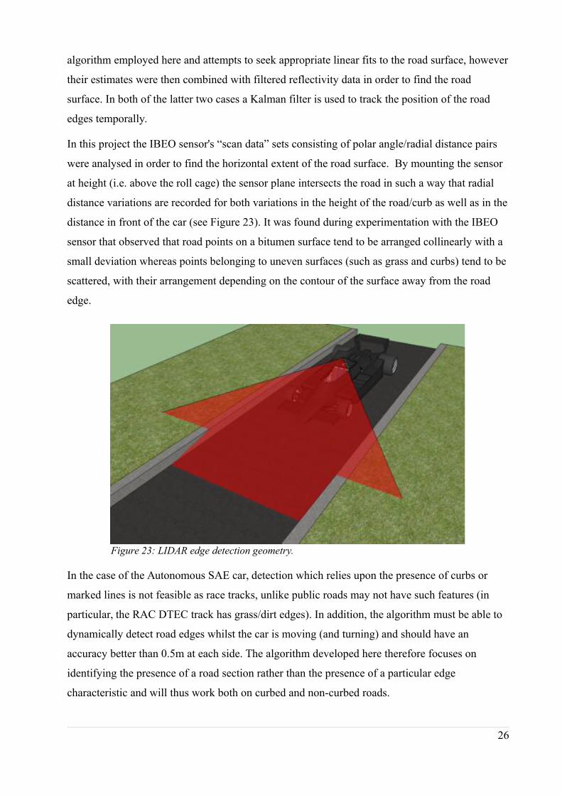
Examples of cases in which these modes were applied are shown below in Figure 25. The yellow

lines indicate the current estimate used, the green diamonds the identified road-edge point and

red points exceed the slope condition.

1 – Reallocated peak

2 – Dip selected

3 – Greatest local maximum

peak

Figure 25: Examples of road-edge identification scenarios.

30

-7 -6 -5 -4 -3 -2 -1 0

0

0.2

0.4

0.6

0.8

1

0 2 4 6 8 10 12

0

0.2

0.4

0.6

0.8

1

Lateral distance (m)

0 2 4 6 8 10 12

0

0.2

0.4

0.6

0.8

1

Lateral distance (m)

Lateral distance (m)

r2

r2

r2

The most important pre-set parameters for this algorithm are the slope condition value and

allowed variation. The slope condition is set based upon the the nature of the road surface and

severity of roll experienced – a lower value is preferable and values in the range 0.2-0.3 are

typical. The allowed variation is generally set at around 1.5m but may be increased if there is

significant expected variation in the road edge position. Limits are placed on the distances both

transversely and laterally as to how far away edges should be found and are set based on the

sensor orientation. Finally, other parameters including the candidate group size and minimum

correlation have been set based upon testing and have been found to be non-critical and do not

need any adjustment based upon driving conditions etc. With this improved algorithm it has been

observed that fine tuning of parameters is generally not required beyond a first approximation.

Mapping of Obstacles

The IBEO sensor also provides automated object detection and classification and provides

information including the objects location, geometry, type, age, velocity and echo point set. This

data is projected onto the car's running map data as “fence posts” in order to mark obstructions in

the path. Despite the sensor returning the a defined centre point for the object, it is the object

echo point data which is used for this purpose, as it reveals more about the shape of objects than

the simple rectangles generated by the sensor. As the object data returned by the sensor is

Cartesian and relative to the sensor itself, a rotation matrix is used to first change the reference

frame before it is project onto the map. Note that the rotation matrix is transposed as the IBEO

notation is opposite to the usual convention. The object point is thus located at:

O '=[sin (θ ) −cos(θ )cos(θ ) −sin(θ ) ]O+ r where r is the car's current position vector.

In order to minimise the quantity of data projected, echo points are replaced by “fence post”

circles of fixed radius which mesh together. The loss of precision in mapping is not of concern in

this application since a safety factor in the order of metres is set with regards to detection of

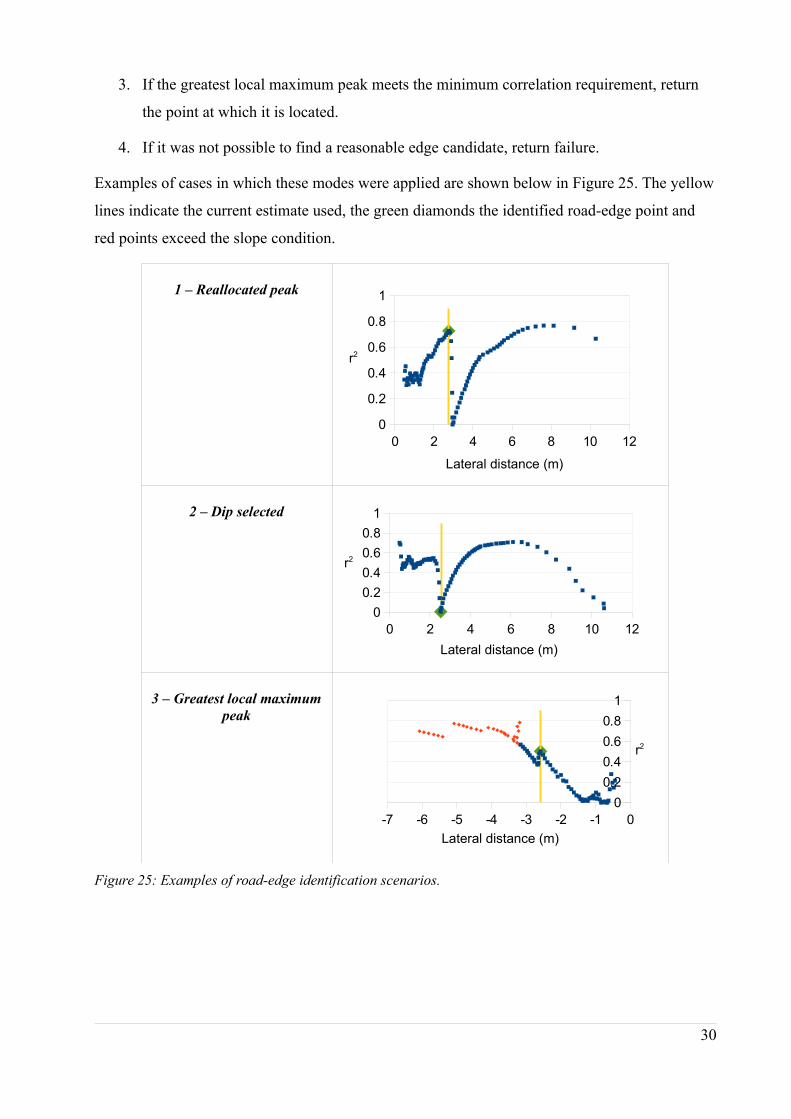
obstructions. The example shown below in Figure 26 shows the detection of building features

outside of the laboratory. At the top left the objects are shown with red markers at their centres

with bounding rectangles overlaid on the raw four-layer scan data (red, orange, yellow, green

respectively) and a detected “road” segment (white) whilst the reduced data set is shown to the

top right.

31

Figure 26: IBEO sensor data (object centres and bounding boxes overlaid on raw scan data), reduced

object data, photograph of scenario. All distances are in metres.

32

5 Instrumentation and Control

5.1 Mapping

Geodesy

In this project, the concept of a “map” is used in order to direct the Autonomous SAE car along a

path made up of waypoints. The map format employed here begins with specification of a datum

- a latitude/longitude pair which is the origin of a local x-y coordinate system. The maps contents

are then specified as x/y pairs in metres relative to the datum, with the y-axis aligned

North-South and the x-axis aligned East-West. It is therefore essential that the distances

calculated on the Cartesian surface bare some resemblance to reality for both informational

purposes and for combination with other data sources. A simplified transformation is used to

convert latitude/longitude inputs, φ and λ respectively, (e.g. from GPS or Google Maps) into

local Cartesian coordinates:

x=RE

2π360

(ϕ −ϕ D)

y=RE

2 π360

cos∣ϕ∣(λ −λ D )

This approach assumes that the Earth's radius is sufficiently large and the angle difference

between the datum and position are sufficiently small that the curvature of the Earth is negligible

in the area local to the Cartesian coordinate system. The accuracy is thus proportional to the

accuracy of the Earth's radius, RE, which is defined in the World Geodetic System 1984 [47] (the

standard utilised by GPS) to be that of an ellipsoid with equatorial semi-major axis 6378.137 km

and flattening factor 298.26. This gives a variation of 21.4 km from minimum to maximum

radius, which corresponds to a 0.34% error, which on the scales (100m) used in this project

would translate to a maximum error of 34cm. However, a better estimate of the local Earth radius

can be obtained based on the geometry of the ellipse:

R=√(a2cos ϕ )

2+(b

2sin ϕ )

2

(acos ϕ )2+(bsin ϕ )2

This gives approximately 6372km and was taken as the value of RE in this project. The error

between the WGS84 ellipsoid and the mean-sea-level is on the order of tens of metres [48], as is

the local (Perth coastal plain) [49] height above mean-sea-level which is relatively small with

respect to the magnitude of the Earth's radius. If a worst case error of 100m was assumed this

now corresponds to an error of 0.0016% which quite clearly acceptable in this project.

33

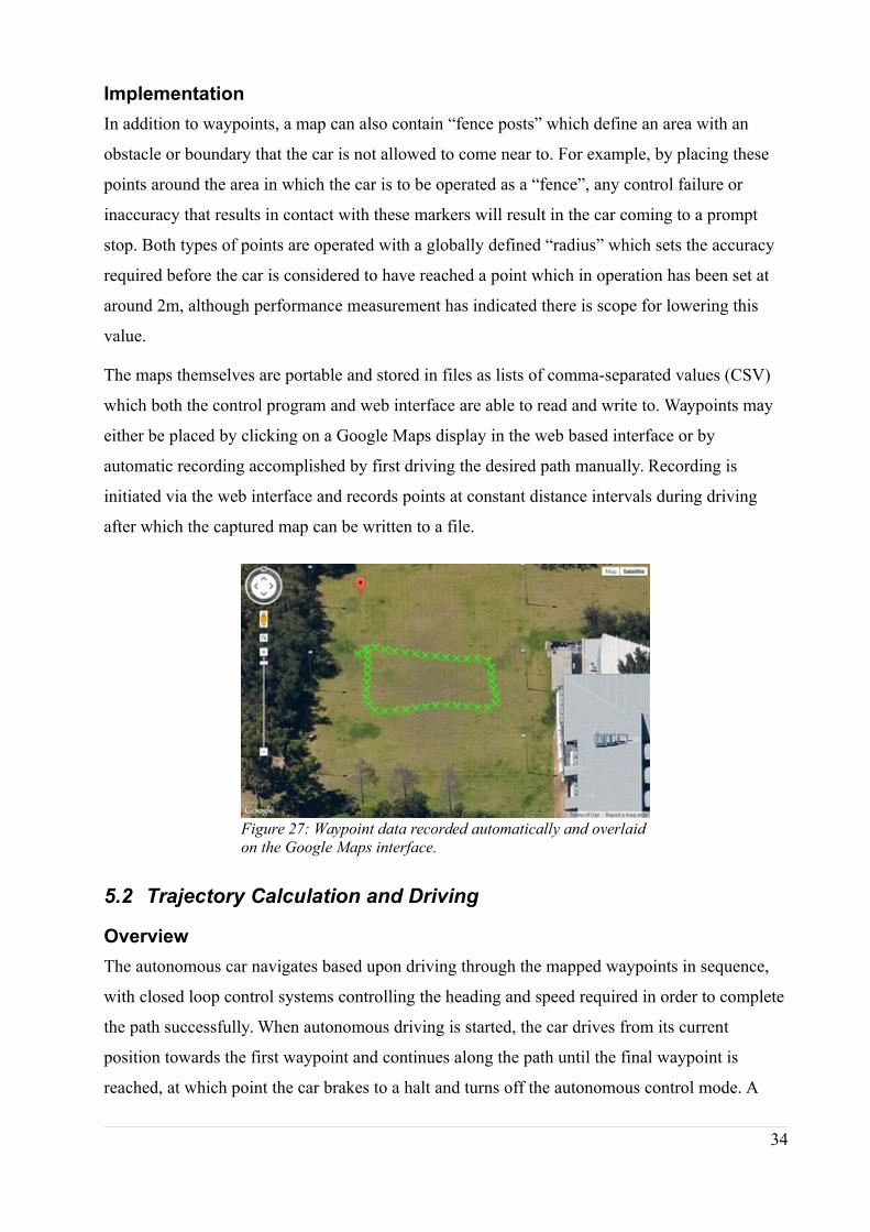
Implementation

In addition to waypoints, a map can also contain “fence posts” which define an area with an

obstacle or boundary that the car is not allowed to come near to. For example, by placing these

points around the area in which the car is to be operated as a “fence”, any control failure or

inaccuracy that results in contact with these markers will result in the car coming to a prompt

stop. Both types of points are operated with a globally defined “radius” which sets the accuracy

required before the car is considered to have reached a point which in operation has been set at

around 2m, although performance measurement has indicated there is scope for lowering this

value.

The maps themselves are portable and stored in files as lists of comma-separated values (CSV)

which both the control program and web interface are able to read and write to. Waypoints may

either be placed by clicking on a Google Maps display in the web based interface or by

automatic recording accomplished by first driving the desired path manually. Recording is

initiated via the web interface and records points at constant distance intervals during driving

after which the captured map can be written to a file.

Figure 27: Waypoint data recorded automatically and overlaid

on the Google Maps interface.

5.2 Trajectory Calculation and Driving

Overview

The autonomous car navigates based upon driving through the mapped waypoints in sequence,

with closed loop control systems controlling the heading and speed required in order to complete

the path successfully. When autonomous driving is started, the car drives from its current

position towards the first waypoint and continues along the path until the final waypoint is

reached, at which point the car brakes to a halt and turns off the autonomous control mode. A

34

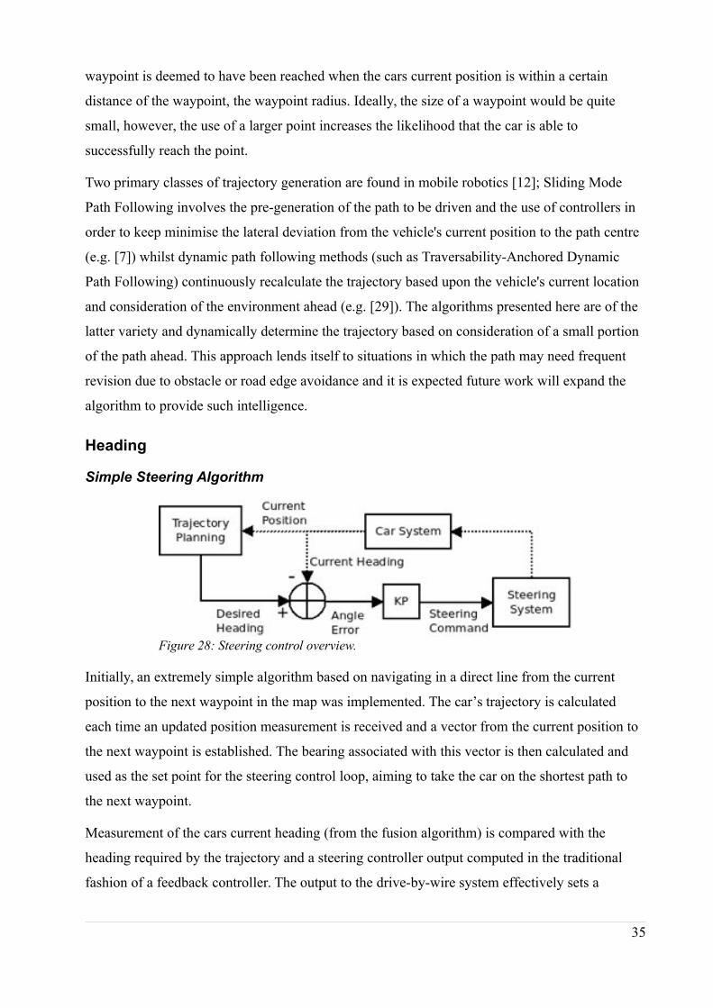
waypoint is deemed to have been reached when the cars current position is within a certain

distance of the waypoint, the waypoint radius. Ideally, the size of a waypoint would be quite

small, however, the use of a larger point increases the likelihood that the car is able to

successfully reach the point.

Two primary classes of trajectory generation are found in mobile robotics [12]; Sliding Mode

Path Following involves the pre-generation of the path to be driven and the use of controllers in

order to keep minimise the lateral deviation from the vehicle's current position to the path centre

(e.g. [7]) whilst dynamic path following methods (such as Traversability-Anchored Dynamic

Path Following) continuously recalculate the trajectory based upon the vehicle's current location

and consideration of the environment ahead (e.g. [29]). The algorithms presented here are of the

latter variety and dynamically determine the trajectory based on consideration of a small portion

of the path ahead. This approach lends itself to situations in which the path may need frequent

revision due to obstacle or road edge avoidance and it is expected future work will expand the

algorithm to provide such intelligence.

Heading

Simple Steering Algorithm

Figure 28: Steering control overview.

Initially, an extremely simple algorithm based on navigating in a direct line from the current

position to the next waypoint in the map was implemented. The car’s trajectory is calculated

each time an updated position measurement is received and a vector from the current position to

the next waypoint is established. The bearing associated with this vector is then calculated and

used as the set point for the steering control loop, aiming to take the car on the shortest path to

the next waypoint.

Measurement of the cars current heading (from the fusion algorithm) is compared with the

heading required by the trajectory and a steering controller output computed in the traditional

fashion of a feedback controller. The output to the drive-by-wire system effectively sets a

35

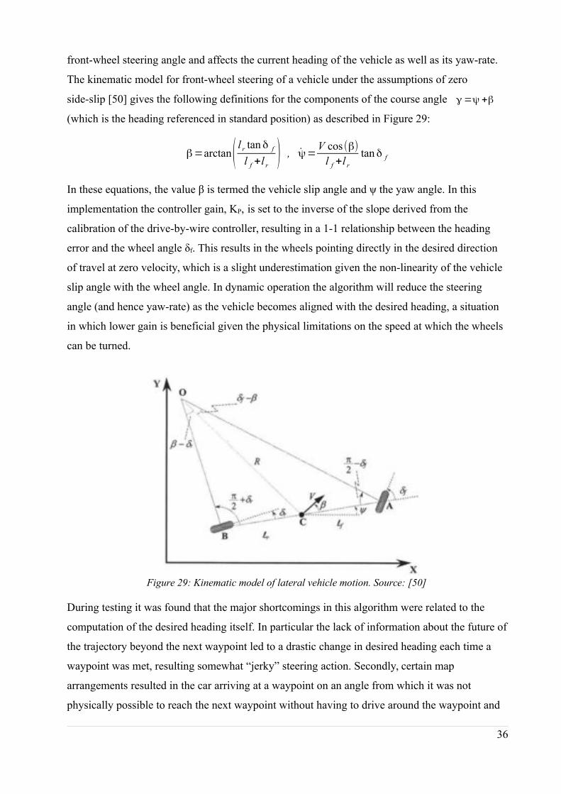
front-wheel steering angle and affects the current heading of the vehicle as well as its yaw-rate.

The kinematic model for front-wheel steering of a vehicle under the assumptions of zero

side-slip [50] gives the following definitions for the components of the course angle γ =ψ +β

(which is the heading referenced in standard position) as described in Figure 29:

β=arctan( l r tan δ f

l f +l r) , ψ=

V cos (β)l f +l r

tan δ f

In these equations, the value β is termed the vehicle slip angle and ψ the yaw angle. In this

implementation the controller gain, KP, is set to the inverse of the slope derived from the

calibration of the drive-by-wire controller, resulting in a 1-1 relationship between the heading

error and the wheel angle δf. This results in the wheels pointing directly in the desired direction

of travel at zero velocity, which is a slight underestimation given the non-linearity of the vehicle

slip angle with the wheel angle. In dynamic operation the algorithm will reduce the steering

angle (and hence yaw-rate) as the vehicle becomes aligned with the desired heading, a situation

in which lower gain is beneficial given the physical limitations on the speed at which the wheels

can be turned.

Figure 29: Kinematic model of lateral vehicle motion. Source: [50]

During testing it was found that the major shortcomings in this algorithm were related to the

computation of the desired heading itself. In particular the lack of information about the future of

the trajectory beyond the next waypoint led to a drastic change in desired heading each time a

waypoint was met, resulting somewhat “jerky” steering action. Secondly, certain map

arrangements resulted in the car arriving at a waypoint on an angle from which it was not

physically possible to reach the next waypoint without having to drive around the waypoint and

36

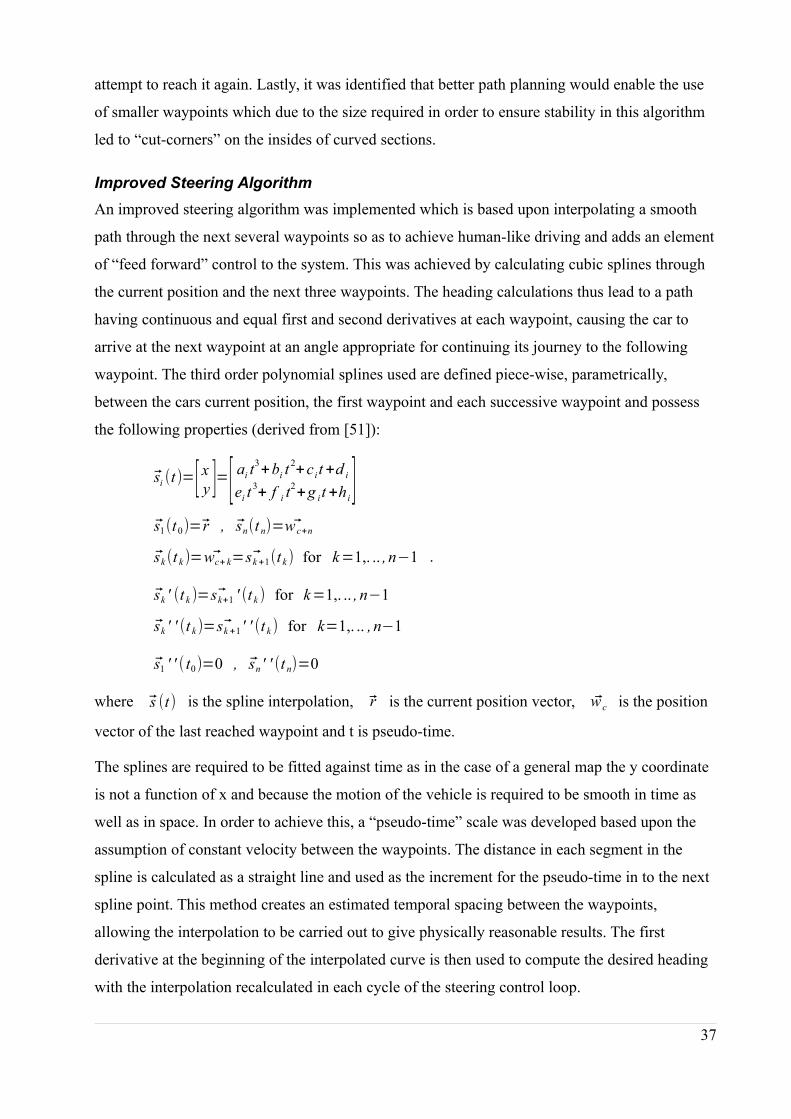
attempt to reach it again. Lastly, it was identified that better path planning would enable the use

of smaller waypoints which due to the size required in order to ensure stability in this algorithm

led to “cut-corners” on the insides of curved sections.

Improved Steering Algorithm

An improved steering algorithm was implemented which is based upon interpolating a smooth

path through the next several waypoints so as to achieve human-like driving and adds an element

of “feed forward” control to the system. This was achieved by calculating cubic splines through

the current position and the next three waypoints. The heading calculations thus lead to a path

having continuous and equal first and second derivatives at each waypoint, causing the car to

arrive at the next waypoint at an angle appropriate for continuing its journey to the following

waypoint. The third order polynomial splines used are defined piece-wise, parametrically,

between the cars current position, the first waypoint and each successive waypoint and possess

the following properties (derived from [51]):

si (t)=[ x

y ]=[ ai t3+bi t

2+cit +d i

ei t3+ f i t

2+g it +hi]

s1(t0)= r , sn(t n)=wc+n

sk (t k )=wc+ k= sk +1(t k ) for k=1,. .. , n−1 .

sk ' (t k )= sk+1 ' (t k ) for k=1,. .. , n−1

sk ' ' (t k)= sk +1 ' ' (t k ) for k=1,. .. , n−1

s1 ' ' ( t0)=0 , sn ' ' (t n)=0

where s (t) is the spline interpolation, r is the current position vector, wc is the position

vector of the last reached waypoint and t is pseudo-time.

The splines are required to be fitted against time as in the case of a general map the y coordinate

is not a function of x and because the motion of the vehicle is required to be smooth in time as

well as in space. In order to achieve this, a “pseudo-time” scale was developed based upon the

assumption of constant velocity between the waypoints. The distance in each segment in the

spline is calculated as a straight line and used as the increment for the pseudo-time in to the next

spline point. This method creates an estimated temporal spacing between the waypoints,

allowing the interpolation to be carried out to give physically reasonable results. The first

derivative at the beginning of the interpolated curve is then used to compute the desired heading

with the interpolation recalculated in each cycle of the steering control loop.

37

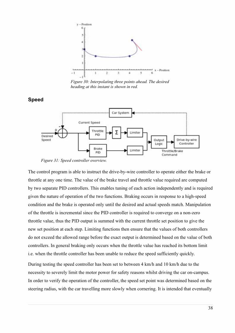
Figure 30: Interpolating three points ahead. The desired

heading at this instant is shown in red.

Speed

The control program is able to instruct the drive-by-wire controller to operate either the brake or

throttle at any one time. The value of the brake travel and throttle value required are computed

by two separate PID controllers. This enables tuning of each action independently and is required

given the nature of operation of the two functions. Braking occurs in response to a high-speed

condition and the brake is operated only until the desired and actual speeds match. Manipulation

of the throttle is incremental since the PID controller is required to converge on a non-zero

throttle value, thus the PID output is summed with the current throttle set position to give the

new set position at each step. Limiting functions then ensure that the values of both controllers

do not exceed the allowed range before the exact output is determined based on the value of both

controllers. In general braking only occurs when the throttle value has reached its bottom limit

i.e. when the throttle controller has been unable to reduce the speed sufficiently quickly.

During testing the speed controller has been set to between 4 km/h and 10 km/h due to the

necessity to severely limit the motor power for safety reasons whilst driving the car on-campus.

In order to verify the operation of the controller, the speed set point was determined based on the

steering radius, with the car travelling more slowly when cornering. It is intended that eventually

38

Figure 31: Speed controller overview.

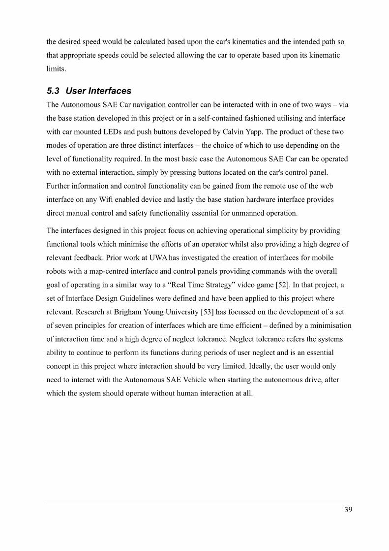
the desired speed would be calculated based upon the car's kinematics and the intended path so

that appropriate speeds could be selected allowing the car to operate based upon its kinematic

limits.

5.3 User Interfaces

The Autonomous SAE Car navigation controller can be interacted with in one of two ways – via

the base station developed in this project or in a self-contained fashioned utilising and interface

with car mounted LEDs and push buttons developed by Calvin Yapp. The product of these two

modes of operation are three distinct interfaces – the choice of which to use depending on the

level of functionality required. In the most basic case the Autonomous SAE Car can be operated

with no external interaction, simply by pressing buttons located on the car's control panel.

Further information and control functionality can be gained from the remote use of the web

interface on any Wifi enabled device and lastly the base station hardware interface provides

direct manual control and safety functionality essential for unmanned operation.

The interfaces designed in this project focus on achieving operational simplicity by providing

functional tools which minimise the efforts of an operator whilst also providing a high degree of

relevant feedback. Prior work at UWA has investigated the creation of interfaces for mobile

robots with a map-centred interface and control panels providing commands with the overall

goal of operating in a similar way to a “Real Time Strategy” video game [52]. In that project, a

set of Interface Design Guidelines were defined and have been applied to this project where

relevant. Research at Brigham Young University [53] has focussed on the development of a set

of seven principles for creation of interfaces which are time efficient – defined by a minimisation

of interaction time and a high degree of neglect tolerance. Neglect tolerance refers the systems

ability to continue to perform its functions during periods of user neglect and is an essential

concept in this project where interaction should be very limited. Ideally, the user would only

need to interact with the Autonomous SAE Vehicle when starting the autonomous drive, after

which the system should operate without human interaction at all.

39

Base Station Driven

Base Station Hardware Interface

The base station hardware interface is designed for minimal human interaction and should

ideally run in the background on the base station computer. The interface itself is broken up into

five separate panels, each concerned with a separate system (e.g. input from USB button, output

to car etc.). A series of coloured panels are used to give a visual indication of the status of

operation, with red indicating a failure, green indication normal operation and grey indication

that the system is not turned on. If manual control of the vehicle is desired – only interaction

with this interface is required as use of the “Force Manual” button will override any other mode

of operation allowing for an efficient transition to manual control with minimum operator effort.

Once started and operation of this system verified, it may be “neglected” by the user during

operation of the vehicle. Any system failures are accompanied by a pop-up message, which

brings this interface back into the users scope of attention as per the principle of “attention

management” identified in [53].

Web Interface

Traditionally robot interfaces have been developed using a variety of graphical toolkits to build

stand-alone PC applications, some specifically designed for a particular robot system [52] and

others which have been designed to be portable [54]. In this project a web-based interface was

developed consisting of dynamic HTML pages delivered by a web server located on the

Autonomous SAE Car itself. This approach has a number of benefits over traditional methods

including reduced development time, familiar user interface paradigm, ease of access and

platform independence. Earlier attempts at robot web interfaces implemented customised

40

Figure 32: Base station control panel interface.

software and focussed on the the applications in long-distance control of robot systems over the

Internet [55] [56], however, more recent work has implemented interfaces based upon

standardised AJAX/HTML [57] techniques for data display.

The interface implemented in this project is specific to the Autonomous SAE Car, but utilises

standard software libraries and techniques, all of which are freely available and easily reused in

other applications. The interface consists of three web pages (see Appendix D), the first of which

is used for generating maps and control of the car. It is again split into functional control panels

and features sections for recording maps by pointing and clicking on the Google Maps interface,

tools for editing existing maps, a listing of the current status of various software parameters,

buttons for sending commands to the vehicle and a display of the control system log. The use of

Google Maps provides a familiar, easy to use, interactive interface, however, a display showing

factors relating to the car's trajectory during autonomous driving was found to be more useful

during execution of the map. This display shows the current position of the car in the local

Cartesian coordinate system, the past and future waypoints on the trajectory and an indication of

the car's actual and desired heading.

The concept of “externalizing memory” [53] has been implemented through two web pages

which allow the replay of data captured during operation. The first displays a RADAR-style plot

of the LIDAR data showing all four layers of scan data, the detected road edges and an overlay

of any detected object regions. Live data is available for testing as well as the ability to view any

previously detected data. Secondly, a web page dedicated to post-drive analysis provides eight

different graphs displaying the behaviour of the trajectory generation algorithms, outputs to the

drive-by-wire system and the cars velocity and path over the course of operation.

This web interface has performed very well during testing with the only practical limitation

being the quality of the Wifi link to the vehicle, however, it should be noted that such a system is

not appropriate for use in safety critical applications, hence the need for parallel implementation

of the base station hardware interface. The interface design appears to have been time efficient

during testing with around five clicks required to record and drive a mapped path. The potential

for customisation and extension of this interface has proven very promising and represents an

exciting opportunity for further improvement.

41

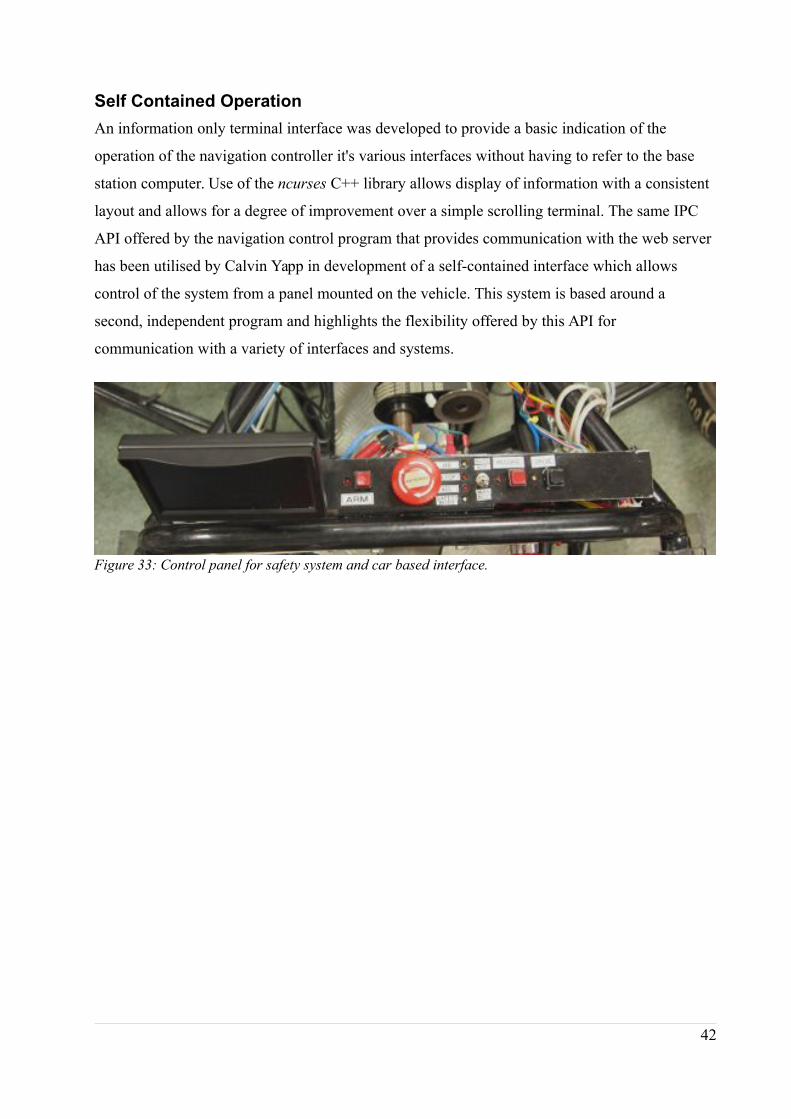
Self Contained Operation

An information only terminal interface was developed to provide a basic indication of the

operation of the navigation controller it's various interfaces without having to refer to the base

station computer. Use of the ncurses C++ library allows display of information with a consistent

layout and allows for a degree of improvement over a simple scrolling terminal. The same IPC

API offered by the navigation control program that provides communication with the web server

has been utilised by Calvin Yapp in development of a self-contained interface which allows

control of the system from a panel mounted on the vehicle. This system is based around a

second, independent program and highlights the flexibility offered by this API for

communication with a variety of interfaces and systems.

42

Figure 33: Control panel for safety system and car based interface.

6 Safety

6.1 Requirements and Design

Risk Assessment

Analysis and identification of risks and design of safety controls was considered as an integral

part of this project due to the hazards associated with autonomous vehicles. Safety standards and

design and verification methodologies for safety related systems [58] are well established for use

in safety-critical systems in industry, however, these systems traditionally do not have the added

complexity of human-robot interaction [59]. Research conducted as part of the Safety-SAM

project [60] identified that system development can be broken into six major stages:

1. Safety analysis

2. Production of a safety requirements specification

3. Hazard partitioning

4. Specification of information requirements of the safety manager

5. System architecture design

6. Prototype development

Safety analysis involves identification of potential hazards and classification of the associated

risks which can then be used to form a set of safety requirements. The hazards are then grouped

together in terms of the systems that will be used to mitigate them allowing specification, design

and implementation of safety systems to take place. An independent safety management system

is typically implemented in order to achieve the safety requirements with a high reliability [59]

[60].

Identification of hazards associated with the Autonomous SAE Car was based on the scenario of

testing speed limited autonomous driving in an open area with members of the public nearby,

however, the system requirements were created with operation at higher speeds in the future in

mind. A variety of techniques exist for hazard identification including the chemical/process

oriented HAZOP technique, SHARD (a variation designed for analysis of software) [59] and

CLASH (a methodology designed for large autonomous vehicles) [60]. In this project, a team

based brainstorming session was undertaken to identify hazards in a similar way to [59] and the

results and requirements were recorded using UWA's risk-register template (see Appendix E).

This analysis revealed that the most important consideration was the ability to detect failure of

control and stop the car and hence the safety systems were designed in a way which seeks to

maximise the reliability of this functionality.

43

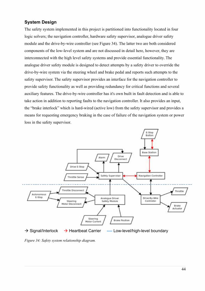
System Design

The safety system implemented in this project is partitioned into functionality located in four

logic solvers; the navigation controller, hardware safety supervisor, analogue driver safety

module and the drive-by-wire controller (see Figure 34). The latter two are both considered

components of the low-level system and are not discussed in detail here, however, they are

interconnected with the high level safety systems and provide essential functionality. The

analogue driver safety module is designed to detect attempts by a safety driver to override the

drive-by-wire system via the steering wheel and brake pedal and reports such attempts to the

safety supervisor. The safety supervisor provides an interface for the navigation controller to

provide safety functionality as well as providing redundancy for critical functions and several

auxiliary features. The drive-by-wire controller has it's own built in fault detection and is able to

take action in addition to reporting faults to the navigation controller. It also provides an input,

the “brake interlock” which is hard-wired (active low) from the safety supervisor and provides a

means for requesting emergency braking in the case of failure of the navigation system or power

loss in the safety supervisor.

à Signal/Interlock à Heartbeat Carrier ---- Low-level/high-level boundary

Figure 34: Safety system relationship diagram.

44

The design for the safety system was based upon two distinct profiles of operation – the first in

which a “safety driver” is present in the vehicle and is able to take action in the case of a loss of

control and the second in which the car drives fully autonomously with no person present. In the

first instance, the ability to remotely stop the car is desirable, but not strictly necessary and so

two safety modes were developed in order to allow more flexibility during operation (e.g.

driving where Wifi is not practical). Thus, in the human driving profile, a trip will not be initiated

when connection between the base station and car is interrupted and autonomous driving will be

able to commence without an active Wifi connection.

In the fully autonomous profile the “heartbeat” signal which originates at the base station and

terminates at the hardware safety supervisor is required to be present. This signal is a 10Hz

binary square wave sampled at 50Hz via the base emergency stop button (see section 3.2) and

transmitted via the TCP/IP over Wifi link to the navigation controller. The navigation controller

then passes the signal onto the safety supervisor over the serial connection as well as performing

verification that the network connection is error free. The safety supervisor measures the time

between heartbeat signals and is able to initiate an emergency stop if the time period exceeds the

set value. As the emergency stop button, base station, Wifi link, navigation controller and serial

connection must all be functioning for this signal to be transmitted in a timely fashion the system

is fail safe and provides protection against a variety of failure scenarios.

6.2 Integrated Safety Features

The navigation controller features integrated error detection and will enter a trip state if any

thread calls the Control::Trip() function. After entering a trip state the navigation controller will

disable autonomous driving, set the accelerator value to zero and send an emergency stop

command to the hardware safety supervisor. Each call to Trip() must be accompanied by a reason

number, which identifies the error message to be recorded in the log to aid diagnosis of faults

(see Table 8 below). The base-station likewise incorporates integrated fault detection and will

automatically send an emergency stop command if the connection to the USB controller fails

while the heartbeat loop through the emergency stop button ensures that failure of the stop button

interface is detected.

45

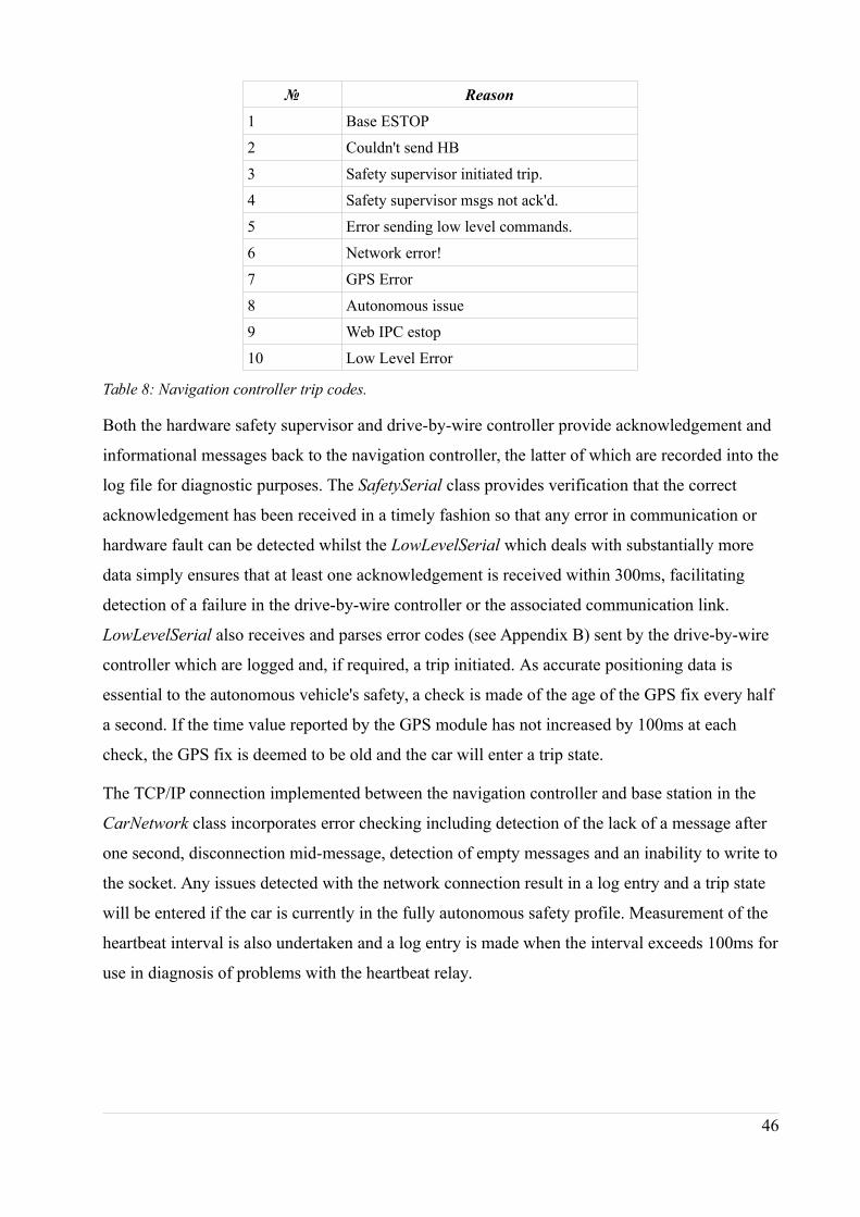
№ Reason

1 Base ESTOP

2 Couldn't send HB

3 Safety supervisor initiated trip.

4 Safety supervisor msgs not ack'd.

5 Error sending low level commands.

6 Network error!

7 GPS Error

8 Autonomous issue

9 Web IPC estop

10 Low Level Error

Table 8: Navigation controller trip codes.

Both the hardware safety supervisor and drive-by-wire controller provide acknowledgement and

informational messages back to the navigation controller, the latter of which are recorded into the

log file for diagnostic purposes. The SafetySerial class provides verification that the correct

acknowledgement has been received in a timely fashion so that any error in communication or

hardware fault can be detected whilst the LowLevelSerial which deals with substantially more

data simply ensures that at least one acknowledgement is received within 300ms, facilitating

detection of a failure in the drive-by-wire controller or the associated communication link.

LowLevelSerial also receives and parses error codes (see Appendix B) sent by the drive-by-wire

controller which are logged and, if required, a trip initiated. As accurate positioning data is

essential to the autonomous vehicle's safety, a check is made of the age of the GPS fix every half

a second. If the time value reported by the GPS module has not increased by 100ms at each

check, the GPS fix is deemed to be old and the car will enter a trip state.

The TCP/IP connection implemented between the navigation controller and base station in the

CarNetwork class incorporates error checking including detection of the lack of a message after

one second, disconnection mid-message, detection of empty messages and an inability to write to

the socket. Any issues detected with the network connection result in a log entry and a trip state

will be entered if the car is currently in the fully autonomous safety profile. Measurement of the

heartbeat interval is also undertaken and a log entry is made when the interval exceeds 100ms for

use in diagnosis of problems with the heartbeat relay.

46

6.3 Hardware Safety Supervisor

The hardware safety supervisor system was created in order to add a level of redundancy to the

car's safety systems. By implementing the system as a self-contained device additional

risk-reduction is achieved compared to integration with the high or low level primary control

systems and is implemented to passively monitor the control systems, human inputs and to

perform independent actions in the event of a trip initiator. The following design specification

was created in order to summarise the required functionality:

Function Importance

Monitor the heartbeat from the high level control system. High

Disconnect drive power in trip condition High

Implement an “arming sequence” and prevent the throttle from activating soon after the drive is enabled

Medium

Apply the brake via a hard-wired signal to the low level controller Medium

Provide audible notification of a fault Medium

Provide feedback as to the state of trip systems Medium

Allow high level control actions based on low-level safety systems Low

Require physical intervention when restarting systems after a fault Low

Table 9: Hardware safety supervisor design requirements.

It was also identified that automatic full-lock braking is inappropriate when the car is in the

“safety driver” profile. In the case of a failure or unexpected event, heavy braking is always the

first response, however a human is able to judge the extent to which this is appropriate in

maintaining stability and coming to a safe stop in an appropriate position. Therefore the system

should cut power to the drive system and relinquish braking and steering to safety to the safety

driver. Thus, an additional desirable criteria is for the hardware safety supervisor to have

awareness of the high level control systems safety profile and to act based on this knowledge.

Hardware

Two possible design solutions were considered for the hardware safety supervisor. An

implementation consisting of only discrete electronic components was initially considered based

upon a missing-pulse detection circuit for monitoring of the heartbeat and an analogue timer

circuit for implementation of an arming sequence. However, despite its increased integrity, such

an approach offers extremely low flexibility and does not scale well. Due to the time required to

develop and test such a system as well as the size of the hardware required in order to implement

all of the functionality discussed above it was decided to consider a micro-controller based

solution instead.

47

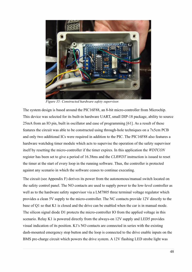
Figure 35: Constructed hardware safety supervisor.

The system design is based around the PIC16F88, an 8-bit micro-controller from Microchip.

This device was selected for its built-in hardware UART, small DIP-18 package, ability to source

25mA from an IO pin, built in oscillator and ease of programming [61]. As a result of these

features the circuit was able to be constructed using through-hole techniques on a 7x5cm PCB

and only two additional ICs were required in addition to the PIC. The PIC16F88 also features a

hardware watchdog timer module which acts to supervise the operation of the safety supervisor

itself by resetting the micro-controller if the timer expires. In this application the WDTCON

register has been set to give a period of 16.38ms and the CLRWDT instruction is issued to reset

the timer at the start of every loop in the running software. Thus, the controller is protected

against any scenario in which the software ceases to continue executing.

The circuit (see Appendix F) derives its power from the autonomous/manual switch located on

the safety control panel. The NO contacts are used to supply power to the low-level controller as

well as to the hardware safety supervisor via a LM7805 three terminal voltage regulator which

provides a clean 5V supply to the micro-controller. The NC contacts provide 12V directly to the

base of Q1 so that K1 is closed and the drive can be enabled when the car is in manual mode.

The silicon signal diode D1 protects the micro-controller IO from the applied voltage in this

scenario. Relay K1 is powered directly from the always-on 12V supply and LED5 provides

visual indication of its position. K1's NO contacts are connected in series with the existing

dash-mounted emergency stop button and the loop is connected to the drive enable inputs on the

BMS pre-charge circuit which powers the drive system. A 12V flashing LED strobe light was

48

installed in parallel with the main drive contractor's coil and mounted on top of the car as per

current Formula-SAE regulations giving an indication of the actual drive status from afar. An

additional bipolar transistor, Q2 drives a piezoelectric transducer which provides a 80dB SPL

alert tone which is activated during trip conditions or remotely as a horn. As the PIC16F88 is

able to source up to 25mA per IO pin, indicator LEDs showing the heartbeat activity, trip

condition, throttle timer condition and safety system profile are able to be driven directly via

current limiting resistors.

The PIC16F88 features an internal oscillator block and in this case it has been configured to run

at 8MHz – it is factory tuned and is typically accurate to ±1% at room temperature, which is

quite sufficient for this application. The hardware safety supervisor receives input from the high

level control system via an inexpensive USB-serial converter module based on the PL2303 IC.

This interface is supported natively under Linux and provides a TTL level interface compatible

with the micro-controller's UART. In this instance the serial communication is implemented at

38400 Baud as this rate is able to be implemented with minimal error utilising the PIC's internal

oscillator;

Baud Rate=F OSC

16( X +1)=

8∗106

16(12+1)=38461.5 [61]

where X is the value written to SPBRG register which configures the serial port.

Extensive use is made of the PIC's built in timer module, TMR0 for checking the period between

heartbeat transitions as well as implementing delays in the arming sequence. The PIC's

OPTION_REG register has been configured so that the timer is interrupted by a signal prescaled

by dividing the instruction clock by 256. The TMR0 counter register is then preset to 100,

resulting in the register overflowing and triggering with frequency:

F intterupt=8∗10

6 /4256∗(256−100)

=50.08 Hz

Thus, timing operations are easily implemented by counting the number of interrupts required

for a desired time interval.

Additional IO is handled using the PICs two IO banks, with bit numbers selected based on the

circuit board layout. Inputs from switch contacts are in a pull-up configuration and switch

de-bouncing is handled in software whilst the normally-high brake interlock output to the

low-level controller is pulled down and loaded with a small capacitor in order to provide a

fail-safe scenario and increase noise immunity respectively. Input from the throttle line to the

49

Kelly motor controllers is applied to an LM358 op-amp configured as a comparator and

compared against an adjustable reference. The output of this is provided to the micro-controller

via an optoisolator as the throttle signal is referenced to the drive train power supply.

Software State Machine

The micro-controller software was developed using MikroElektronika's ANSI C PIC Compiler

suite and takes the basis of a state-machine design. The software accomplishes four primary

functions; monitoring the heartbeat signal, acting upon trips initiated by the navigation

controller, reporting trips initiated by the analogue hardware safety module and allowing for safe

“arming” of the autonomous system. The micro-controller continuously receives commands

consisting of a single ASCII character (see Table 10) from the navigation controller via its UART

and sends reply messages consisting on a variable length string followed by the new-line

character.

Command Description

E Emergency stop

+ Heartbeat high value

- Heartbeat low value

B Set brake interlock on (fully autonomous safety profile)

H Set brake interlock off (human safety driver profile)

A Sound piezo alarm

Table 10: Hardware Safety Supervisor Command Set

The arming sequence is designed to mitigate the risk associated with the possibility of the car

accelerating due to hardware or software failure in the time period immediately following

enabling the drive system. A sequenced start-up has been implemented which operates as

follows:

1. Operator holds arm button

2. Full brake is applied

3. After 4s the drive system is enabled and throttle sensor turned on.

4. After a further 4s the operator can release the arm button – any premature release will

disconnect the drive.

5. After 10s the brake releases.

6. After a further 2s the throttle sensor is disabled.

50

This means that the arm button must be held for a total of 8s for the drive to stay enabled and

protects against accidental start-up. The 4s delay after the drive is enabled before latching

provides the operator an opportunity to disconnect the drive power simply by letting go of the

button if something goes wrong immediately after the drive is enabled. If a throttle voltage is

detected within 16s of the drive being enabled the drive will also be disabled giving the operator

time to move away from the car before it is possible for it to start moving. A lack of heartbeat

signal or trip condition initiated by the navigation controller, analogue driver safety module or

dash emergency stop will result in the drive being disabled and alarm activated.

The implementation of this functionality consists of a set of states with associated outputs and

transition conditions, with the identity of the current state contained in an integer variable (see

Appendices G and H for the state diagram and output table). The program's main loop consists of

receiving input from the UART and performing any actions required based upon it (such as

resetting the heartbeat timer), followed by evaluating the conditions required for transition from

the current state into another. Extensive informational messages are relayed to the navigation

system during arming and when a fault is detected as well as acknowledgement responses for

each command received over the serial link.

This system has performed well and required minimal adjustment, however, the maximum

allowed interval between heartbeat transitions had to be increased beyond the desired 200ms

(chosen to give a maximum travel of around 3m before stopping at 50km/h) in order to achieve

stable operation. It was found that whilst the safety supervisor was capable of this interval the

Wifi connection to the base-station was not able to meet this specification reliably and as a result

the interval was increased to 600ms. The cause of this issue is mostly likely interference from

other 2.4GHz networks at UWA as the Wifi transceivers used are designed to work at the

distances involved in this project. This has not caused an issue as testing has been carried out at

speeds significantly lower than 50km/h, however in the future this issue will need further

examination.

51

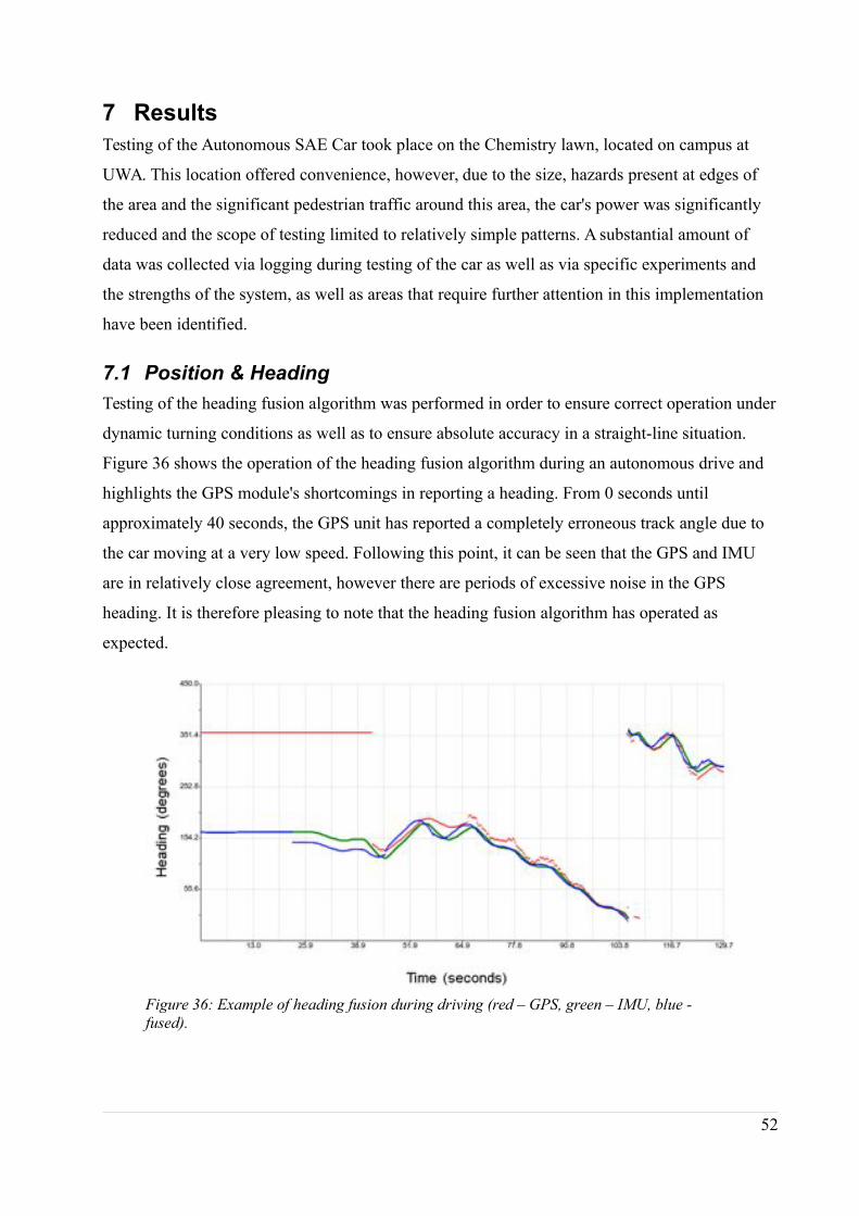
7 Results

Testing of the Autonomous SAE Car took place on the Chemistry lawn, located on campus at

UWA. This location offered convenience, however, due to the size, hazards present at edges of

the area and the significant pedestrian traffic around this area, the car's power was significantly

reduced and the scope of testing limited to relatively simple patterns. A substantial amount of

data was collected via logging during testing of the car as well as via specific experiments and

the strengths of the system, as well as areas that require further attention in this implementation

have been identified.

7.1 Position & Heading

Testing of the heading fusion algorithm was performed in order to ensure correct operation under

dynamic turning conditions as well as to ensure absolute accuracy in a straight-line situation.

Figure 36 shows the operation of the heading fusion algorithm during an autonomous drive and

highlights the GPS module's shortcomings in reporting a heading. From 0 seconds until

approximately 40 seconds, the GPS unit has reported a completely erroneous track angle due to

the car moving at a very low speed. Following this point, it can be seen that the GPS and IMU

are in relatively close agreement, however there are periods of excessive noise in the GPS

heading. It is therefore pleasing to note that the heading fusion algorithm has operated as

expected.

Figure 36: Example of heading fusion during driving (red – GPS, green – IMU, blue -

fused).

52

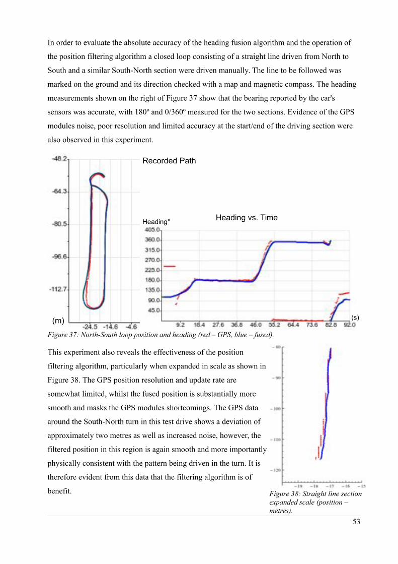
In order to evaluate the absolute accuracy of the heading fusion algorithm and the operation of

the position filtering algorithm a closed loop consisting of a straight line driven from North to

South and a similar South-North section were driven manually. The line to be followed was

marked on the ground and its direction checked with a map and magnetic compass. The heading

measurements shown on the right of Figure 37 show that the bearing reported by the car's

sensors was accurate, with 180º and 0/360º measured for the two sections. Evidence of the GPS

modules noise, poor resolution and limited accuracy at the start/end of the driving section were

also observed in this experiment.

Figure 37: North-South loop position and heading (red – GPS, blue – fused).

This experiment also reveals the effectiveness of the position

filtering algorithm, particularly when expanded in scale as shown in

Figure 38. The GPS position resolution and update rate are

somewhat limited, whilst the fused position is substantially more

smooth and masks the GPS modules shortcomings. The GPS data

around the South-North turn in this test drive shows a deviation of

approximately two metres as well as increased noise, however, the

filtered position in this region is again smooth and more importantly

physically consistent with the pattern being driven in the turn. It is

therefore evident from this data that the filtering algorithm is of

benefit.

53

(m)

Recorded Path

Heading vs. TimeHeading°

(s)

Figure 38: Straight line section

expanded scale (position –

metres).

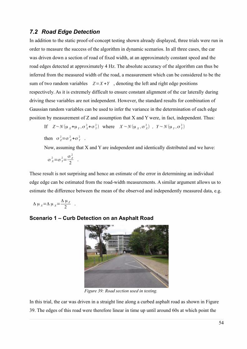
7.2 Road Edge Detection

In addition to the static proof-of-concept testing shown already displayed, three trials were run in

order to measure the success of the algorithm in dynamic scenarios. In all three cases, the car

was driven down a section of road of fixed width, at an approximately constant speed and the

road edges detected at approximately 4 Hz. The absolute accuracy of the algorithm can thus be

inferred from the measured width of the road, a measurement which can be considered to be the

sum of two random variables Z=X +Y , denoting the left and right edge positions

respectively. As it is extremely difficult to ensure constant alignment of the car laterally during

driving these variables are not independent. However, the standard results for combination of

Gaussian random variables can be used to infer the variance in the determination of each edge

position by measurement of Z and assumption that X and Y were, in fact, independent. Thus:

If Z~N (μ X +μ Y ,σ X

2 +σ Y

2 ) where X ~N (μ X ,σ X

2 ) , Y ~N (μ Y ,σ Y

2 )

then σZ

2=σX

2 +σY

2 .

Now, assuming that X and Y are independent and identically distributed and we have:

σ X

2 =σ Y

2=σ Z

2

2.

These result is not surprising and hence an estimate of the error in determining an individual

edge edge can be estimated from the road-width measurements. A similar argument allows us to

estimate the difference between the mean of the observed and independently measured data, e.g.

Δ μ X=Δ μ X=Δ μ Z

2.

Scenario 1 – Curb Detection on an Asphalt Road

Figure 39: Road section used in testing.

In this trial, the car was driven in a straight line along a curbed asphalt road as shown in Figure

39. The edges of this road were therefore linear in time up until around 60s at which point the

54

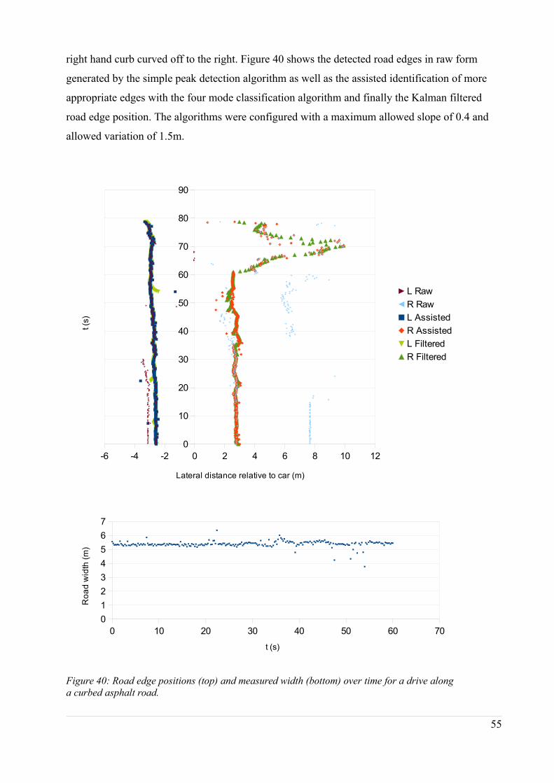
right hand curb curved off to the right. Figure 40 shows the detected road edges in raw form

generated by the simple peak detection algorithm as well as the assisted identification of more

appropriate edges with the four mode classification algorithm and finally the Kalman filtered

road edge position. The algorithms were configured with a maximum allowed slope of 0.4 and

allowed variation of 1.5m.

-6 -4 -2 0 2 4 6 8 10 12

0

10

20

30

40

50

60

70

80

90

L Raw

R Raw

L Assisted

R Assisted

L Filtered

R Filtered

Lateral distance relative to car (m)

t (s

)

0 10 20 30 40 50 60 70

0

1

2

3

4

5

6

7

t (s)

Ro

ad

wid

th (

m)

Figure 40: Road edge positions (top) and measured width (bottom) over time for a drive along

a curbed asphalt road.

55

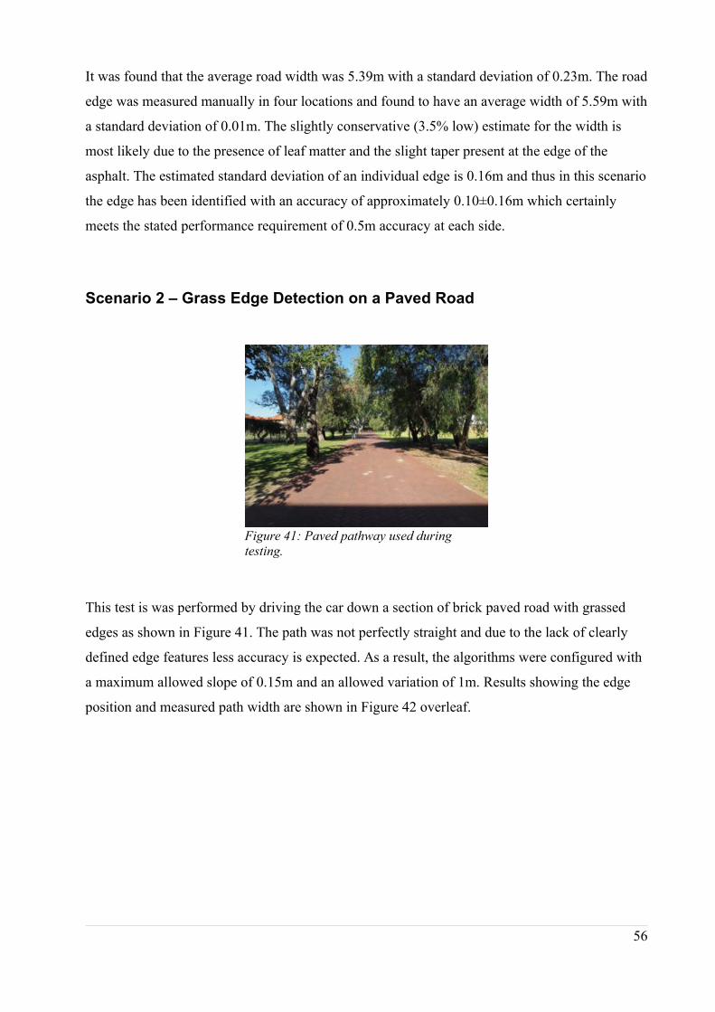
It was found that the average road width was 5.39m with a standard deviation of 0.23m. The road

edge was measured manually in four locations and found to have an average width of 5.59m with

a standard deviation of 0.01m. The slightly conservative (3.5% low) estimate for the width is

most likely due to the presence of leaf matter and the slight taper present at the edge of the

asphalt. The estimated standard deviation of an individual edge is 0.16m and thus in this scenario

the edge has been identified with an accuracy of approximately 0.10±0.16m which certainly

meets the stated performance requirement of 0.5m accuracy at each side.

Scenario 2 – Grass Edge Detection on a Paved Road

Figure 41: Paved pathway used during

testing.

This test is was performed by driving the car down a section of brick paved road with grassed

edges as shown in Figure 41. The path was not perfectly straight and due to the lack of clearly

defined edge features less accuracy is expected. As a result, the algorithms were configured with

a maximum allowed slope of 0.15m and an allowed variation of 1m. Results showing the edge

position and measured path width are shown in Figure 42 overleaf.

56

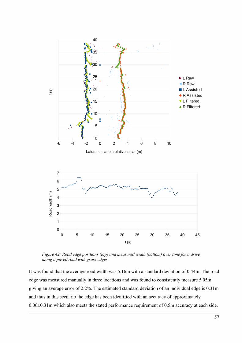
-6 -4 -2 0 2 4 6 8 10

0

5

10

15

20

25

30

35

40

L Raw

R Raw

L Assisted

R Assisted

L Filtered

R Filtered

Lateral distance relative to car (m)

t (s

)

0 5 10 15 20 25 30 35 40 45

0

1

2

3

4

5

6

7

t (s)

Ro

ad

wid

th (

m)

Figure 42: Road edge positions (top) and measured width (bottom) over time for a drive

along a paved road with grass edges.

It was found that the average road width was 5.16m with a standard deviation of 0.44m. The road

edge was measured manually in three locations and was found to consistently measure 5.05m,

giving an average error of 2.2%. The estimated standard deviation of an individual edge is 0.31m

and thus in this scenario the edge has been identified with an accuracy of approximately

0.06±0.31m which also meets the stated performance requirement of 0.5m accuracy at each side.

57

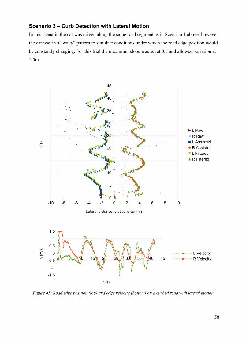
Scenario 3 – Curb Detection with Lateral Motion

In this scenario the car was driven along the same road segment as in Scenario 1 above, however

the car was in a “wavy” pattern to simulate conditions under which the road edge position would

be constantly changing. For this trial the maximum slope was set at 0.5 and allowed variation at

1.5m.

58

-10 -8 -6 -4 -2 0 2 4 6 8 10

0

5

10

15

20

25

30

35

40

45

L Raw

R Raw

L Assisted

R Assisted

L Filtered

R Filtered

Lateral distance relative to car (m)

t (s

)

0 5 10 15 20 25 30 35 40 45

-1.5

-1

-0.5

0

0.5

1

1.5

L Velocity

R Velocity

t (s)

v (

m/s

)

Figure 43: Road edge position (top) and edge velocity (bottom) on a curbed road with lateral motion.

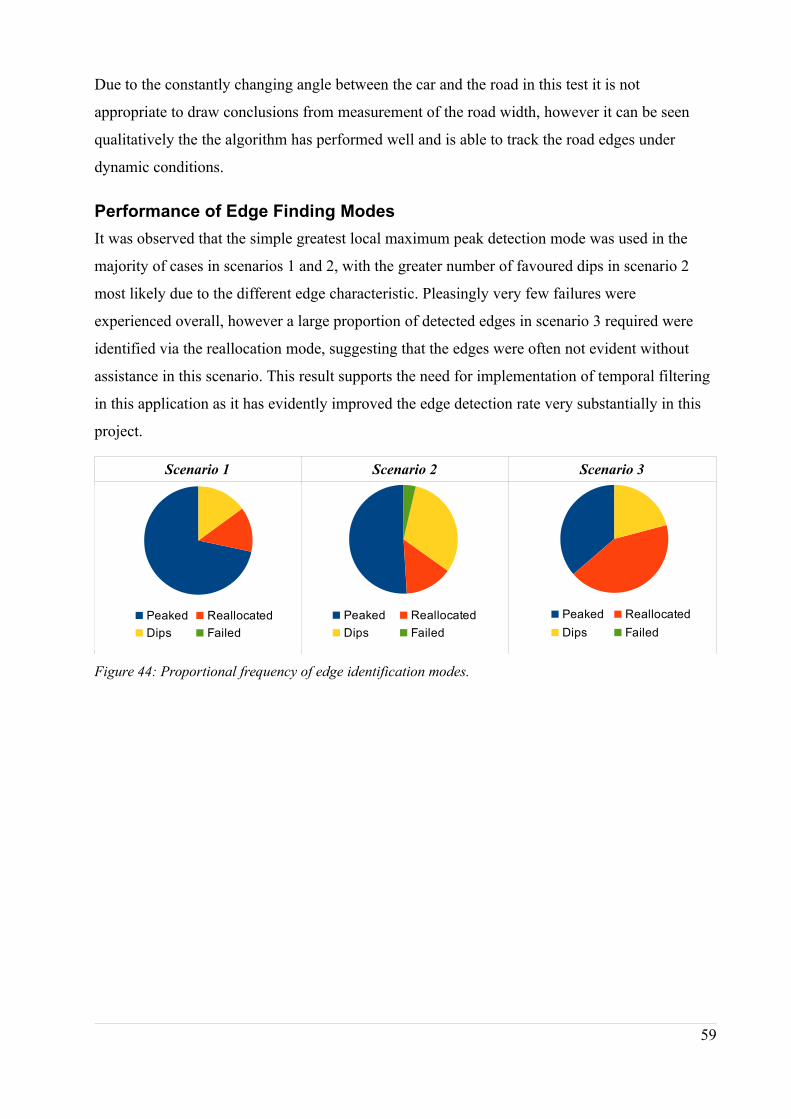
Due to the constantly changing angle between the car and the road in this test it is not

appropriate to draw conclusions from measurement of the road width, however it can be seen

qualitatively the the algorithm has performed well and is able to track the road edges under

dynamic conditions.

Performance of Edge Finding Modes

It was observed that the simple greatest local maximum peak detection mode was used in the

majority of cases in scenarios 1 and 2, with the greater number of favoured dips in scenario 2

most likely due to the different edge characteristic. Pleasingly very few failures were

experienced overall, however a large proportion of detected edges in scenario 3 required were

identified via the reallocation mode, suggesting that the edges were often not evident without

assistance in this scenario. This result supports the need for implementation of temporal filtering

in this application as it has evidently improved the edge detection rate very substantially in this

project.

Scenario 1 Scenario 2 Scenario 3

Peaked Reallocated

Dips Failed

Peaked Reallocated

Dips Failed

Peaked Reallocated

Dips Failed

Figure 44: Proportional frequency of edge identification modes.

59

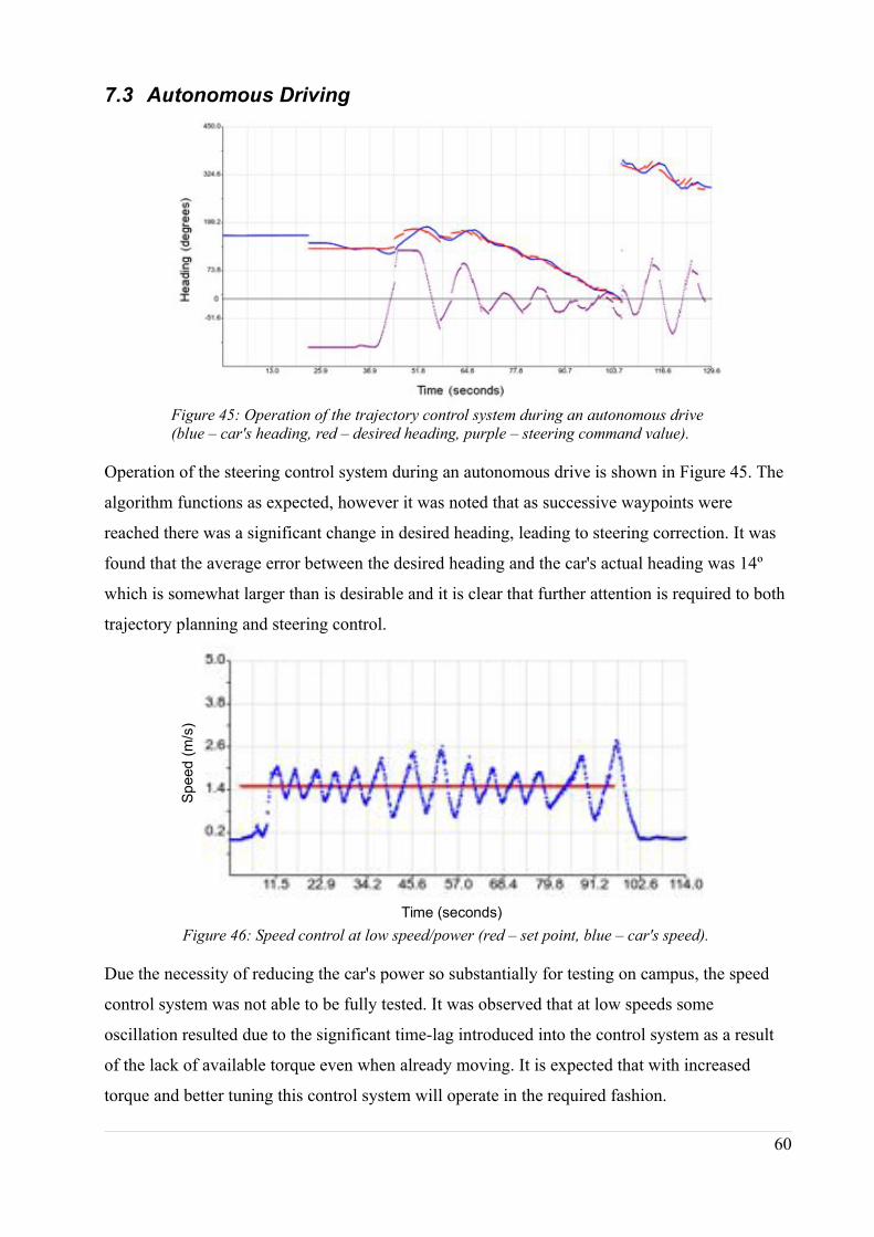
7.3 Autonomous Driving

Figure 45: Operation of the trajectory control system during an autonomous drive

(blue – car's heading, red – desired heading, purple – steering command value).

Operation of the steering control system during an autonomous drive is shown in Figure 45. The

algorithm functions as expected, however it was noted that as successive waypoints were

reached there was a significant change in desired heading, leading to steering correction. It was

found that the average error between the desired heading and the car's actual heading was 14º

which is somewhat larger than is desirable and it is clear that further attention is required to both

trajectory planning and steering control.

Figure 46: Speed control at low speed/power (red – set point, blue – car's speed).

Due the necessity of reducing the car's power so substantially for testing on campus, the speed

control system was not able to be fully tested. It was observed that at low speeds some

oscillation resulted due to the significant time-lag introduced into the control system as a result

of the lack of available torque even when already moving. It is expected that with increased

torque and better tuning this control system will operate in the required fashion.

60

Time (seconds)

Sp

eed

(m

/s)

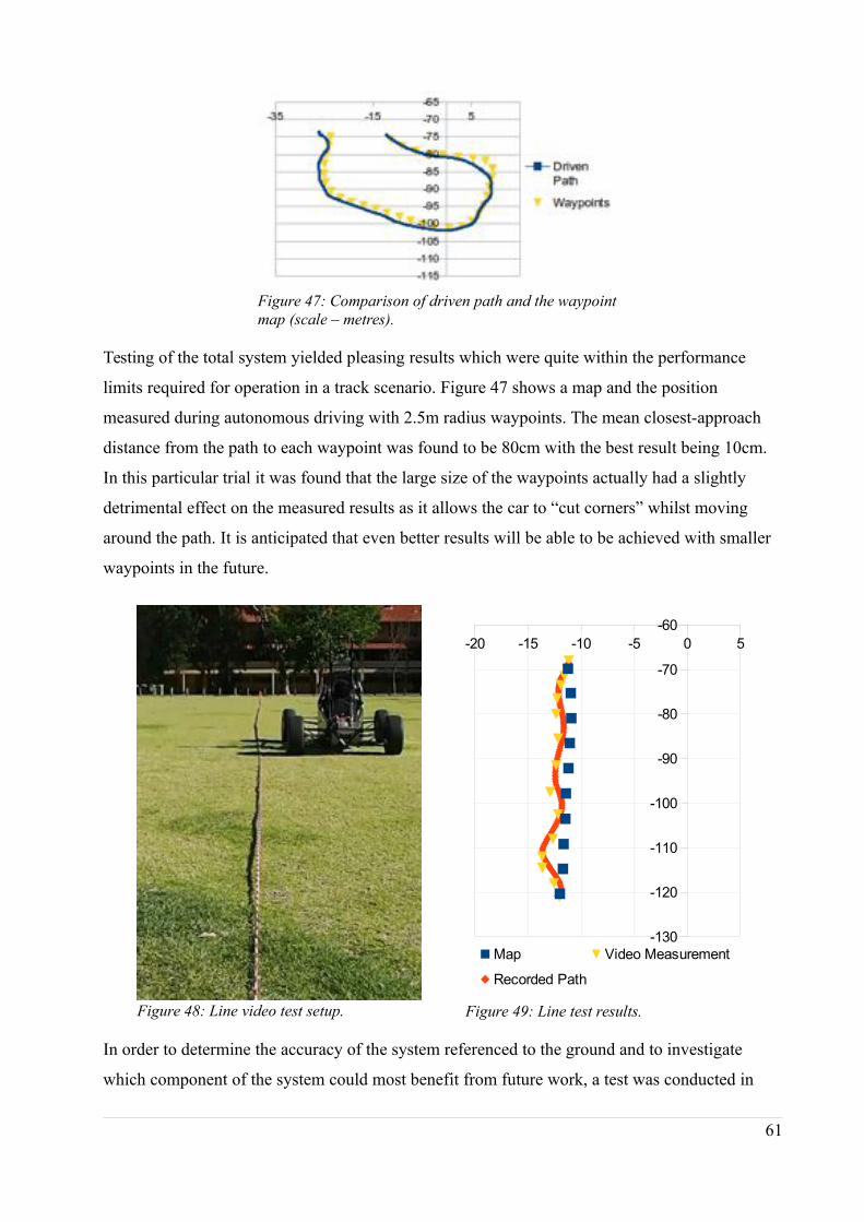
Figure 47: Comparison of driven path and the waypoint

map (scale – metres).

Testing of the total system yielded pleasing results which were quite within the performance

limits required for operation in a track scenario. Figure 47 shows a map and the position

measured during autonomous driving with 2.5m radius waypoints. The mean closest-approach

distance from the path to each waypoint was found to be 80cm with the best result being 10cm.

In this particular trial it was found that the large size of the waypoints actually had a slightly

detrimental effect on the measured results as it allows the car to “cut corners” whilst moving

around the path. It is anticipated that even better results will be able to be achieved with smaller

waypoints in the future.

Figure 48: Line video test setup.

Figure 49: Line test results.

In order to determine the accuracy of the system referenced to the ground and to investigate

which component of the system could most benefit from future work, a test was conducted in

61

-20 -15 -10 -5 0 5

-130

-120

-110

-100

-90

-80

-70

-60

Map Video Measurement

Recorded Path

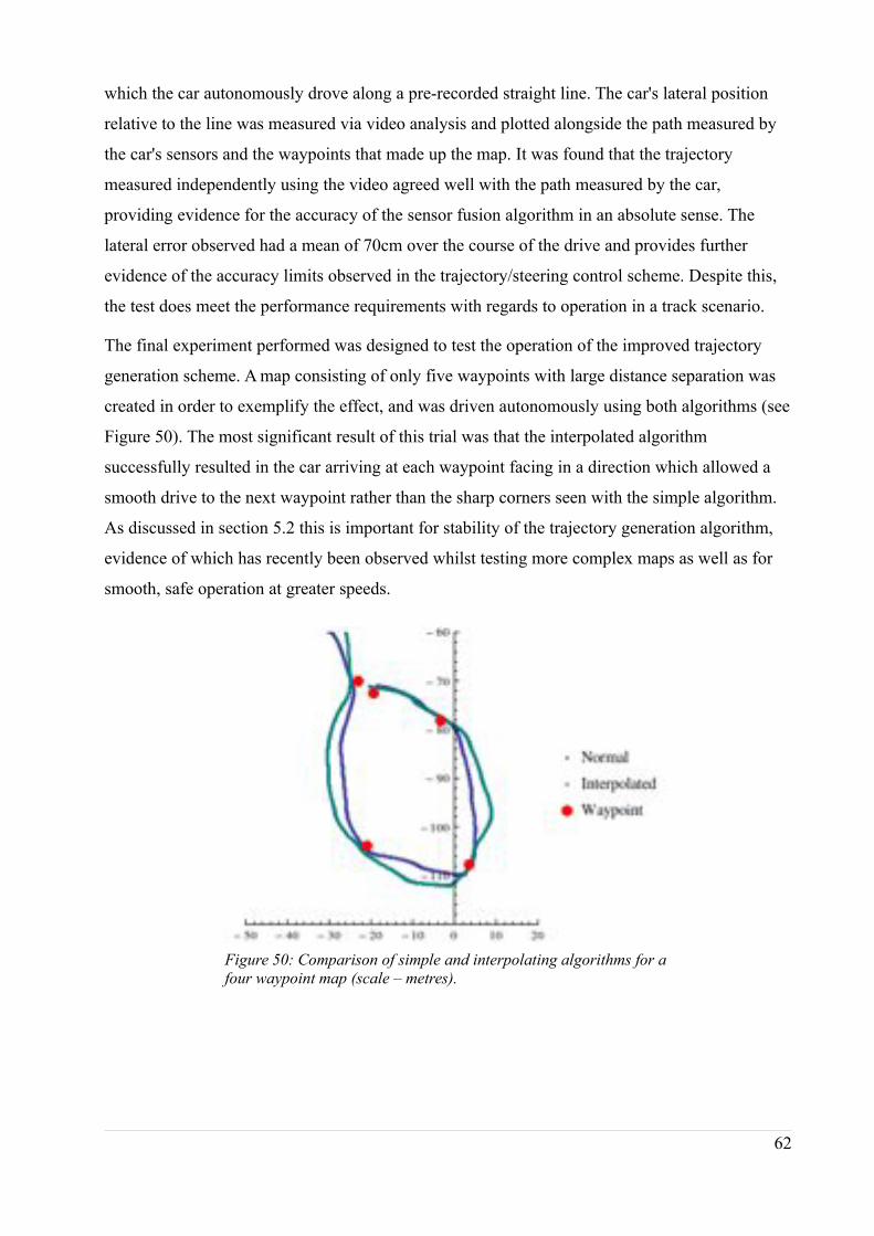
which the car autonomously drove along a pre-recorded straight line. The car's lateral position

relative to the line was measured via video analysis and plotted alongside the path measured by

the car's sensors and the waypoints that made up the map. It was found that the trajectory

measured independently using the video agreed well with the path measured by the car,

providing evidence for the accuracy of the sensor fusion algorithm in an absolute sense. The

lateral error observed had a mean of 70cm over the course of the drive and provides further

evidence of the accuracy limits observed in the trajectory/steering control scheme. Despite this,

the test does meet the performance requirements with regards to operation in a track scenario.

The final experiment performed was designed to test the operation of the improved trajectory

generation scheme. A map consisting of only five waypoints with large distance separation was

created in order to exemplify the effect, and was driven autonomously using both algorithms (see

Figure 50). The most significant result of this trial was that the interpolated algorithm

successfully resulted in the car arriving at each waypoint facing in a direction which allowed a

smooth drive to the next waypoint rather than the sharp corners seen with the simple algorithm.

As discussed in section 5.2 this is important for stability of the trajectory generation algorithm,

evidence of which has recently been observed whilst testing more complex maps as well as for

smooth, safe operation at greater speeds.

Figure 50: Comparison of simple and interpolating algorithms for a

four waypoint map (scale – metres).

62

8 Conclusion and Future Work

Conclusion

This project shows significant promise as a platform for the development of autonomous driving

technology and it is anticipated that with development of the underlying systems completed

future work will focus on refining and improving the methods presented here. The project has

achieved its goal of creating an operational and fully featured control system which allows the

Autonomous SAE Car to drive maps with accuracy and safety appropriate for future testing on a

race track.

The modular design of the software provides the ability to easily modify or implement new

functionality and the hardware systems installed on the vehicle have proven robust. The sensor

array implemented successfully provides sufficient information of a quality useful for driving in

a variety of scenarios. In particular, the sensor fusion algorithms implemented have allowed the

use of comparatively low-cost devices in a demanding application. The road-edge detection

system has achieved excellent results on curbed roads as well as extending the scope of such

systems to roads without a clearly defined edge through tight integration of predictive filtering

with the edge detection algorithm.

The user interfaces developed in this project have been tested and utilised extensively over the

course of this year and have proven to provide powerful functionality as well as valuable tools

for testing and refinement of the Autonomous SAE Car. The use of an asynchronous

web-interface for robotics applications has been validated and it is evident that this technique has

a strong future in the field. Safety has been actively considered throughout this project and the

systems which have now been implemented provide mitigation of a wide variety of hazards in a

manner which is robust, reliable and complements the operation of the vehicle.

The control systems implemented in this project have provided successful operation during

testing and have seen the creation of a framework for control of the vehicle as well as improving

understanding of the requirements for more advanced algorithms. The revised interpolating

trajectory generation algorithm shows significant promise as the basis for more advanced

methods and future work on this project will encompass optimisation of driving behaviours so

that race grade performance can be achieved in the near future.

63

Future Work

There is significant scope for future work on this project now that the hardware and software

platforms necessary for more advanced functionality have been developed and tested. The range

of possible future projects involving the Autonomous SAE Car include improvements to sensor

and communications systems, development of more advanced trajectory calculation and steering

algorithms, further intelligent driving and mapping functionality as well as research into the

operation of autonomous vehicles in traffic scenarios. The variety and scope of such work is

substantial and should see the Autonomous SAE Car operated as a productive research tool for

many years to come.

Potential improvements to the hardware platform would involve the integration of a better

performing Wifi system, selection of a new GPS unit and the addition of image processing to the

system. A communication system which would give reliable performance at distances up to 1 km

and offer better immunity to interference would be extremely beneficial – in particular the new

800 MHz offerings from Ubiquity Networks [62] would be worth investigation. A more

advanced GPS or GPS/INS combination unit such as the MTi-G-700 discussed in section 4.2 or,

when available, an open source RTK solution such as the Piksi [63] would allow safer, more

accurate, navigation and increase the flexibility of the vehicle. Image processing through the

integration of a good quality video camera would also provide opportunities for greater

functionality and research into the problem of fusing LIDAR and video data.

The development of optimised trajectory calculations with a greater level of pre-planning such

that the “racing-line” is able to maximise speed and minimise distance over the course of the

track would be extremely beneficial to this project. In addition to this, the steering and speed

control algorithms could be improved through better characterisation of the dynamics of the

Autonomous SAE Car to achieve performance at the limits of the vehicles abilities. An

opportunity exists for the integration of dynamic map re-planning based on obstacle detection

and ultimately the development of robotic driving algorithms which would operate without

having a pre-defined map. In the foreseeable future this vehicle could be extended to navigate

entirely based upon sensory inputs, with the goal of achieving total autonomy.

64

References

[1] SAE International. “About Formula SAE Series” [Online]. Available:

http://students.sae.org/cds/formulaseries/about.htm. [Accessed: Oct. 20, 2013]

[2] T. Black. “A Driver Assistance System for a BMW X5.” BE thesis, UWA, 2012.

[3] Siemens AG (2007). “Tailored Solutions – Driverless Subways” [Online]. Available:

http://www.siemens.com/innovation/en/publikationen/publications_pof/pof_spring_2008/tailored

_solutions/fahrerlose_ubahn.htm. [Accessed: Oct. 14, 2013]

[4] Rio Tinto Ltd. (2012, Feb.). “Rio Tinto invests US$518 million in autonomous trains for

Pilbara iron ore rail network in Western Australia” [Online]. Available:

http://www.riotinto.com.au/ENG/media/38_media_releases_1743.asp. [Accessed: Oct. 14, 2013]

[5] BBC (2013, Apr.). “Robot truck platoons roll forward” [Online]. Available:

http://www.bbc.com/future/story/20130409-robot-truck-platoons-roll-forward. [Accessed: Oct.

14, 2013]

[6] Ernst D. Dickmanns. “The development of machine vision for road vehicles in the last

decade”, Intelligent Vehicle Symposium, pp. 268-281, 2002.

[7] S. Thrun, M. Montemerlo, H. Dahllamp et. al. “Stanley: The Robot That Won the DARPA

Grand Challenge” in The 2005 DARPA Grand Challenge, M. Buelher, K. Iagnemma, S. Signh,

Eds., Berlin: Springer, 2007, pp. 1-43.

[8] I. Miller, S. Lupashin, N. Zych et. al. “Cornell university's 2005 DARPA grand challenge

entry”, Journal of Field Robotics, vol. 23, no. 8, pp 625-652, Aug. 2006.

[9] M. Montemerlo, J. Becker, H. Dahikamp, D. Dolgov, S. Ettinger, D. Haehnel, T. Hilden, G.

Hoffmann, B. Huhnke, D. Johnson, S. Klumpp, D. Langer, A. Levandowski, J. Levinson, J.

Marcil, D. Orenstein, J. Paefgen, I. Penny, A. Petrovskaya, M. Pflueger. “Junior: The Stanford

entry in the Urban Challenge”, Journal Of Field Robotics, vol. 25, no. 9, pp. 569-597, 2008.

[10] J. Bohren, T. Foote, J. Keller et. al. “Little Ben: The Ben Franklin Racing Team's entry in

the 2007 DARPA Urban Challenge”, Journal of Field Robotics, vol. 25, no. 9, pp. 598-614, Sep.

2008.

[11] A. Bacha, C. Bauman, R. Faruque et. al. “Odin: Team VictorTango's entry in the DARPA

Urban Challenge”, Journal of Field Robotics, vol. 25, no. 8, pp. 467-492, Aug. 2008.

[12] A. Broggi, P. Medici, P. Zani, A. Coati, M. Panciroli. Autonomous vehicles control in the

65

VisLab Intercontinental Autonomous Challenge, Annu. Reviews in Control, vol. 36, no. 1, pp.

161-171, Apr. 2012.

[13] J. Markoff. “Google Cars Drive Themselves, in Traffic”, The New York Times, Oct. 9, 2010

[Online]. Available: http://www.nytimes.com/2010/10/10/science/10google.html. [Accessed:

Aug. 17, 2013]

[14] Electronic News Publishing. “Komatsu and Rio Tinto Enter into Agreement for 150

Autonomous Truck Deployment into Pilbara Iron Ore operations by 2015”, ENP Newswire, 4

Nov. 2011.

[15] Komatsu Australia. “Autonomous Haul System” [Online]. Available:

http://www.komatsu.com.au/AboutKomatsu/Technology/Pages/AHS.aspx [Accessed: Mar. 14,

2013]

[16] Adnan Shaout, Dominic Colella, S. Awad. “Advanced Driver Assistance Systems Past,

Present and Future”. Seventh International Computer Engineering Conference, pp. 72-82, 2011.

[17] Maximillian Muffert, David Pfeiffer, Uwe Franke. “A Stereo-Vision Based Object Tracking

Approach at Roundabouts”. IEEE Intelligent Transport Systems Magazine, Vol 5, Issue 2, pp.

22-32, Apr. 2013.

[18] Kirstin L.R. Talvala, Krisada Kritayakirana, J. Christian Gerdes. “Pushing the limits: From

lanekeeping to autonomous racing”, Annu. Reviews in Control, vol. 35, no. 1, pp. 137-148, Apr.

2011.

[19] Jan Seigemund, Uwe Franke, Wolfgang Forstner. “A temporal filter approach for detection

and reconstruction of curbs and road surfaces based on Conditional Random Fields”. 2011 IEEE

Intelligent Vehicles Symposium, pp 637-642, Jun. 2011.

[20] Vicente Milanés, David F. Llorca, Blas M. Vinagre, Carlos González, Miguel A. Sotelo.

“Clavileño: Evolution of an Autonomous Car”, Annu. Conf. Intelligent Transportation Systems,

Madeira Island, Portugal, pp. 1129-1134, 2010.

[21] L. Brown. “Improving Performance Using Torque Vectoring on an Electric All-Wheel-Drive

Formula SAE Race Car.” BE thesis, UWA, 2013.

[22] T. Brown. “Handling at the limits”, GPS World, vol. 21, no. 8, pp. 38-41, Aug. 2010.

[23] G. Gomez-Gil, S. Alonso-Garcia, F. J. Gomez-Gil, T. Stombaugh. “A Simple Method to

Improve Autonomous GPS Positioning for Tractors”, Sensors, vol. 11, no. 6, pp. 5630-5644,

66

May 2011.

[24] Wende Zhang. “LIDAR-Based Road and Road-Edge Detection”. 2010 IEEE Intelligent

Vehicles Symposium, pp 845-848, Jun. 2010.

[25] B. Fardi, U. Scheunert, H. Cramer, G. Wanielik. “Multi Model Detection and

Parameter-based Tracking of Road Borders with a Laser Scanner”, IEEE IV2003 Intelligent

Vehicles Symposium, pp. 95-99, Jun. 2003.

[26] W.S. Wijesoma, K. R. S. Kodagoda, Arjuna P. Balasuriya. “Road-Boundary Detection and

Tracking Using Ladar Sensing”, IEEE Transactions on Robotics and Automation, vol. 20, no. 3,

Jun. 2004.

[27] B. Dodson. (2012, Nov 11). “Autonomous Audi almost matches veteran race car drivers' lap

times” [Online]. Available:

http://www.gizmag.com/stanford-audi-tts-autonomous-car-thunderhill/24957/. [Accessed: Apr. 7,

2013].

[28] J. Eng. “Implementation of an Embedded System For Vehicle Avoidance For a BMW X5

System”, BE thesis, UWA, 2011.

[29] M. Himmelsbach, F. v. Hundelshausen, T. Luttel, M. Manz, A. Muller, S. Schneider, H.-J.

Wunsche (2009). “Team MuCAR-3 at C-ELROB 2009”, Proceedings of 1st Workshop on Field

Robotics, Civilian European Land Robot Trial 2009 [Online] Available:

http://www.ee.oulu.fi/research/robotics/celrob2009/workshop/papers/Team%20MuCAR-3.pdf.

[Accessed: Jun. 30, 2013]

[30] National Coordination Office for Space-Based Positioning, Navigation and Timing (2013,

Oct 16). “GPS Accuracy” [Online]. Available:

http://www.gps.gov/systems/gps/performance/accuracy/. [Accessed: Jun. 24, 2013].

[31] USU/NASA Geospatial Extension Program (2010, Mar.). “High-End DGPS and RTK

systems” [Online]. Available: http://extension.usu.edu/nasa/files/uploads/gtk-tuts/rtk_dgps.pdf.

[Accessed: Sep. 3, 2013].

[32] Applanix (2010, Aug.). “POS LV Position and Orientation System for Land Vehicles”

[Online]. Available:

http://www.applanix.com/media/downloads/products/brochures/poslv_brochure.pdf. [Accessed:

Apr. 5, 2013]

[33] QStarz. “BT-Q818X User's Manual” [Online]. Available:

67

http://www.qstarz.com/download/BT-Q818X-Users%20Manual.pdf. [Accessed: Sep. 3, 2013].

[34] D. Hennerström. “Increasing GPS Accuracy for Low Cost Receivers”, MSc Thesis, Luleå

University of Technology, 2006.

[35] Xsens Technologies B.V. (2010, Oct.).“MTi and MTx User Manual and Technical

Documentation” [Online]. Available:

http://www.xsens.com/images/stories/products/manual_download/Mti_and_Mtx_User_Manual_

and_Technical_Documentation.pdf. [Accessed: Mar. 6, 2013]

[36] T. C. Henderson, M. Dekhil, R. R. Kessler, M. L. Griss. “Sensor fusion” in Control

Problems in Robotics and Automation, B. Sicilliano, K. P. Valavanis, Eds. Berlin: Springer, 1998,

pp. 193-207.

[37] Marzullo, K. “Tolerating failures of continuous-valued sensors”, ACM Transactions on

Computer Systems, vol. 8, no. 4, pp 284-304, 1990.

[38] W. Elmenreich. “Fusion of Continous-valued Sensor Measurements using

Confidence-weighted Averaging”, Journal of Vibration and Control, vol. 13, no. 9-10, pp.

1303-1312, Sep. 2007.

[39] Xsens Technologies B.V. “MTi-G-700 GPS/INS” [Online]. Available:

http://www.xsens.com/en/general/mti-g-100-series. [Accessed: Mar. 18, 2013]

[40] M. Abe. Vehicle Handling Dynamics Theory and Application. Burlington: Elsevier Science

& Technology, 2009, pp. 5-7.

[41] G. Welch, G. Bishop (2006, Jul.). “An Introduction to the Kalman Filter” [Online].

Available: http://www.cs.unc.edu/~welch/media/pdf/kalman_intro.pdf. [Accessed: Oct. 2, 2013]

[42] O. Robescu. “Assessment of low-cost INS for positioning through sensor fusion with GPS”,

MSc thesis, Chalmers University of Technology [Online]. Available:

http://publications.lib.chalmers.se/records/fulltext/129978.pdf. [Accessed: Jun. 15, 2013]

[43] G. Falco, G. A. Einicke, J. T. Malos, F. Dovis. “Performance Analysis of Constrained

Loosely Coupled GPS/INS Integration Solutions”, Sensors, vol. 12, no. 11, pp. 15983-16007,

Nov. 2012.

[44] Yong Li, Jinling Wang, Chris Rizos, Peter Mumford, Weidong Ding. “Low-cost Tightly

Coupled GPS/INS Integration Based on a Nonlinear Kalman Filtering Design”. Proceedings of

the 2006 National Technical Meeting of The Institute of Navigation, Monterey, CA, pp. 958-966,

68

Jan. 2006.

[45] Honghui Qi, John B. Moore. “Direct Kalman filtering approach for GPS/INS integration”.

IEEE Transactions on Aerospace and Electronic Systems, Vol 38, no. 2, pp. 687-693, Apr. 2002.

[46] ibeo Automotive Systems GmbH (2013, Sep.). “IBEO Lux Datasheet” [Online]. Available:

http://www.ibeo-as.com/ibeo_lux.html. [Accessed: Sep. 30, 2013]

[47] National Imagery and Mapping Agency (2000, Jan.). “Department of Defense World

Geodetic System 1984” [Online]. Available:

http://earth-info.nga.mil/GandG/publications/tr8350.2/wgs84fin.pdf. [Accessed: May 15, 2013]

[48] W. Fraczek. “Mean Sea Level, GPS, and the Geoid”, ArcUser [Online], July-September

2003. Available: http://wou.edu/las/physci/taylor/g492/geoid.pdf. [Accessed: Oct 10, 2013]

[49] Geoscience Australia. “Map Connect – 250K Topographic Map” [Online]. Available:

http://www.ga.gov.au/topographic-mapping/mapconnect.html. [Accessed: Oct 10, 2013]

[50] R. Rajamani. Vehicle Dynamics and Control. New York: Springer-Verlag, 2006, ch. 2.

[51] S. Haque. GENG2140 Lecture, Curve Fitting: “Spline Interpolation”. UWA, Semester 2,

2012.

[52] L. Poli. “User Interface for a Group of Mobile Robots” BE thesis, UWA, 2013.

[53] M.A. Goodrich, D.R. (Jr.) Olsen. “Seven principles of efficient human robot interaction”,

IEEE International Conference on Systems, Man and Cybernetics 2003, vol. 4, pp. 3943-3948,

Oct. 2003.

[54] J. Kock, M. Reichardt, K. Berns. “Universal Web Interfaces for Robot Control

Frameworks”, 2008 IEEE/RSJ International Conference on Intelligent Robots and Systems, pp.

2336-2341, Sep. 2008.

[55] D. Hazry, M. Sugisaka, T. Yuji. “Human-Robot Interface over the Web Based Intelligent

System”, American Journal of Applied Sciences, vol. 3, pp. 1634-1639, Jan. 2006.

[56] S. Mootien, R. T. F. Ah King, H. C. S. Rughooputh. “A Web-Based Interface for the

Gryphon Robot”, 2004 IEEE International Conference on Industrial Technology, vol. 2, pp.

842-847, Dec. 2004.

[57] C. Paolini, G K. Lee. “A Web-Based User Interface for a Mobile Robotic System”, 2012

IEEE International Conference on IRI, pp. 45-50, Aug. 2012.

[58] D. J. Smith, K. G. L. Simpson. Safety Critical Systems Handbook. Oxford: Elsevier Science,

69

2010.

[59] R. Woodman, A. F. T. Winfield, C. Harper, M. Fraser. “Building safer robots: Safety driven

control”, International Journal of Robotics Research, vol. 31, no. 13, Nov. 2012.

[60] D. W. Seward, F.W. Margrave, I. Sommerville, G. Kotony. “Safe Systems for Mobile

Robots – The Safe-SAM Project” in Achievement and Assurance of Safety: Proceedings of the

Third Safety-critical Systems Symposium, F. Redmill, T. Andserson, Eds. London: Springer,

1995, pp. 153-170.

[61] Microchip Technology (2013, May). “PIC16F87/88 Datasheet” [Online]. Available:

http://ww1.microchip.com/downloads/en/DeviceDoc/30487D.pdf. [Accessed: Sep. 17, 2013]

[62] Ubiquiti Networks. “NanoStationM” [Online]. Available:

http://www.ubnt.com/airmax#nanostationm. [Accessed: Oct. 18, 2013]

[63] Swift Navigation Inc. “Piksi: The RTK GPS Receiver” [Online]. Available:

http://www.kickstarter.com/projects/swiftnav/piksi-the-rtk-gps-receiver. [Accessed: Oct. 18,

2013]

70

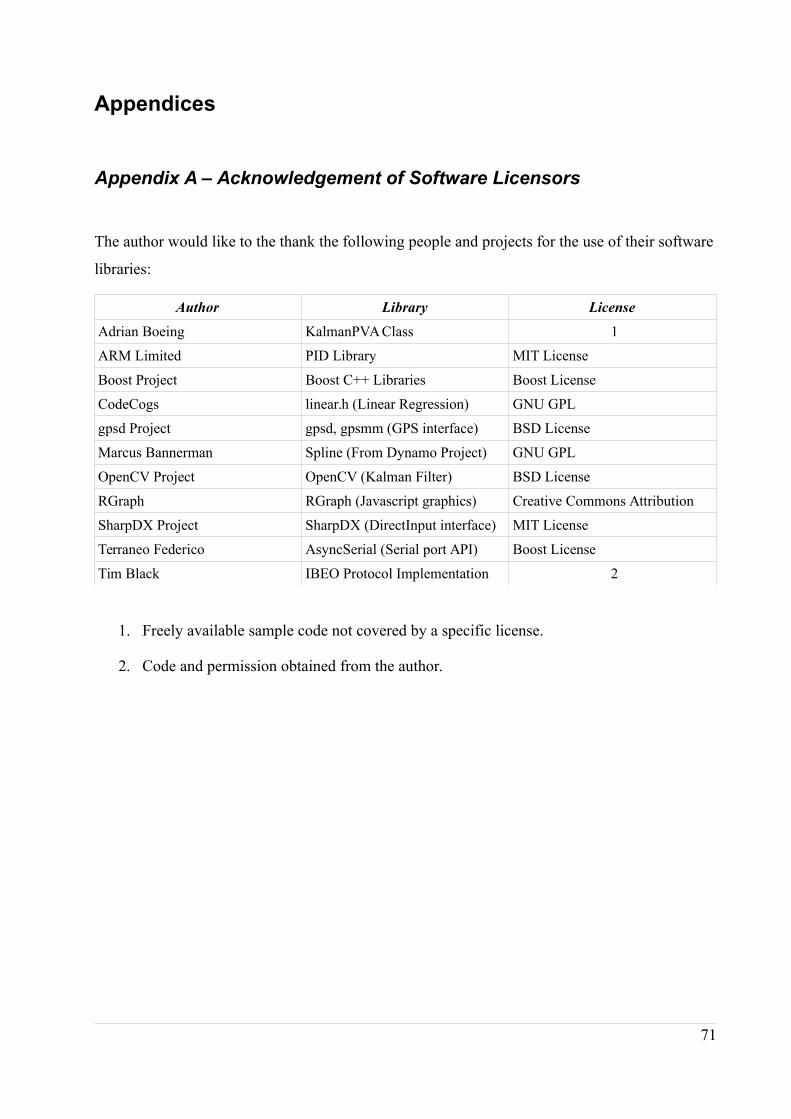
Appendices

Appendix A – Acknowledgement of Software Licensors

The author would like to the thank the following people and projects for the use of their software

libraries:

Author Library License

Adrian Boeing KalmanPVA Class 1

ARM Limited PID Library MIT License

Boost Project Boost C++ Libraries Boost License

CodeCogs linear.h (Linear Regression) GNU GPL

gpsd Project gpsd, gpsmm (GPS interface) BSD License

Marcus Bannerman Spline (From Dynamo Project) GNU GPL

OpenCV Project OpenCV (Kalman Filter) BSD License

RGraph RGraph (Javascript graphics) Creative Commons Attribution

SharpDX Project SharpDX (DirectInput interface) MIT License

Terraneo Federico AsyncSerial (Serial port API) Boost License

Tim Black IBEO Protocol Implementation 2

1. Freely available sample code not covered by a specific license.

2. Code and permission obtained from the author.

71

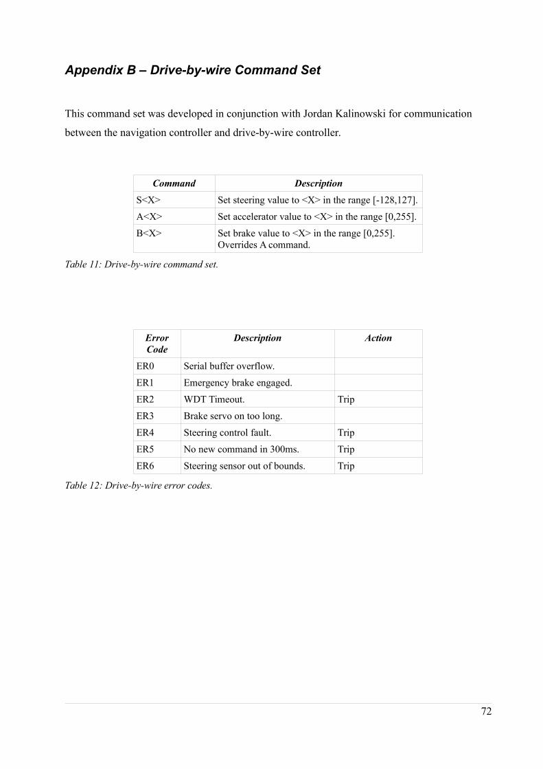
Appendix B – Drive-by-wire Command Set

This command set was developed in conjunction with Jordan Kalinowski for communication

between the navigation controller and drive-by-wire controller.

Command Description

S<X> Set steering value to <X> in the range [-128,127].

A<X> Set accelerator value to <X> in the range [0,255].

B<X> Set brake value to <X> in the range [0,255]. Overrides A command.

Table 11: Drive-by-wire command set.

Error

Code

Description Action

ER0 Serial buffer overflow.

ER1 Emergency brake engaged.

ER2 WDT Timeout. Trip

ER3 Brake servo on too long.

ER4 Steering control fault. Trip

ER5 No new command in 300ms. Trip

ER6 Steering sensor out of bounds. Trip

Table 12: Drive-by-wire error codes.

72

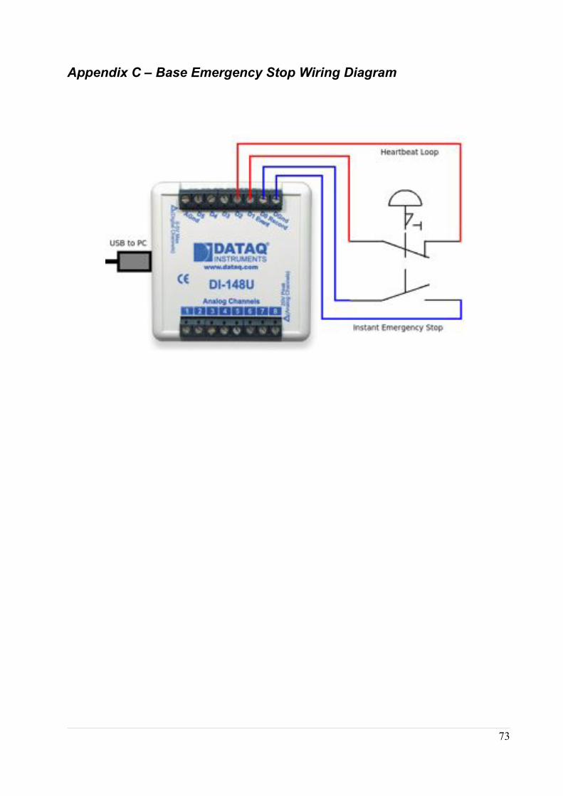
Appendix C – Base Emergency Stop Wiring Diagram

73

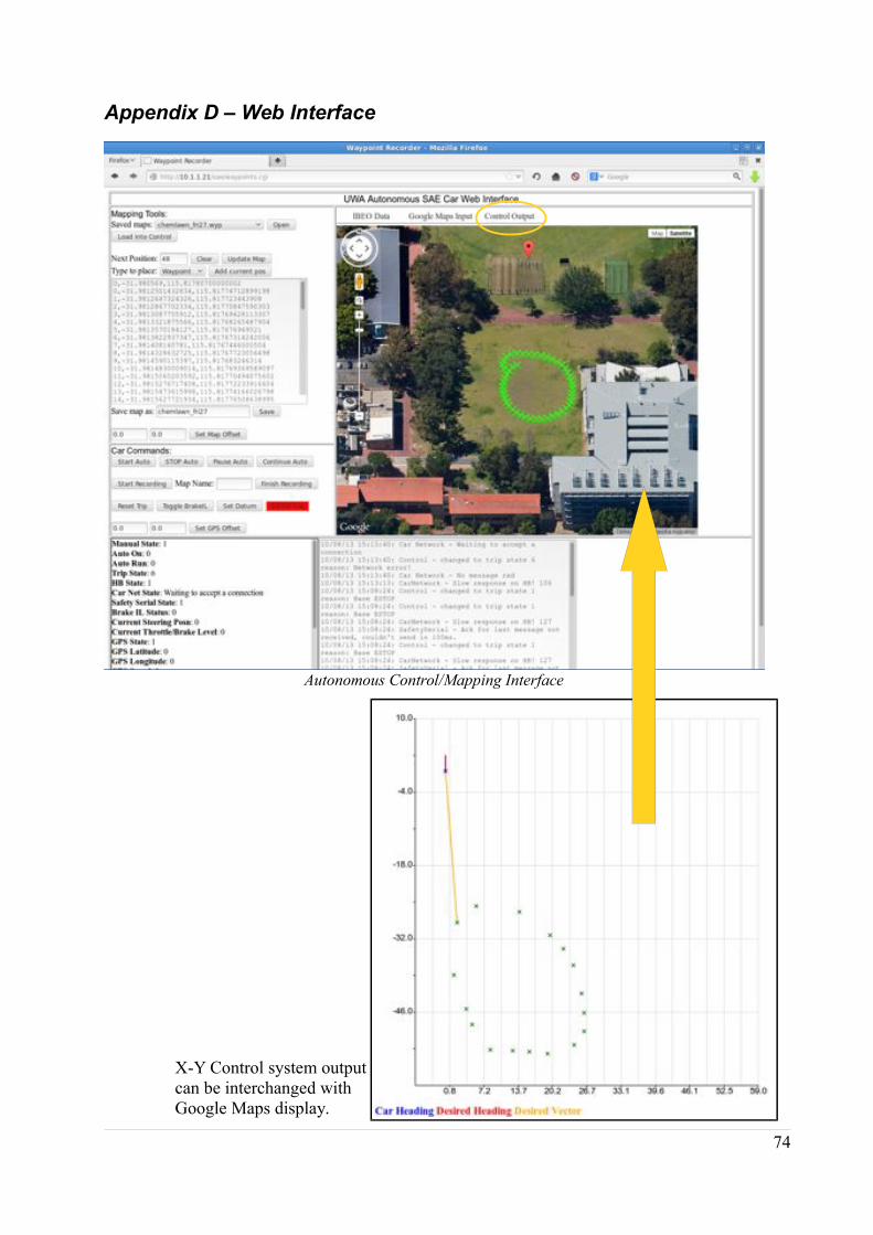
Appendix D – Web Interface

Autonomous Control/Mapping Interface

74

X-Y Control system output can be interchanged with Google Maps display.

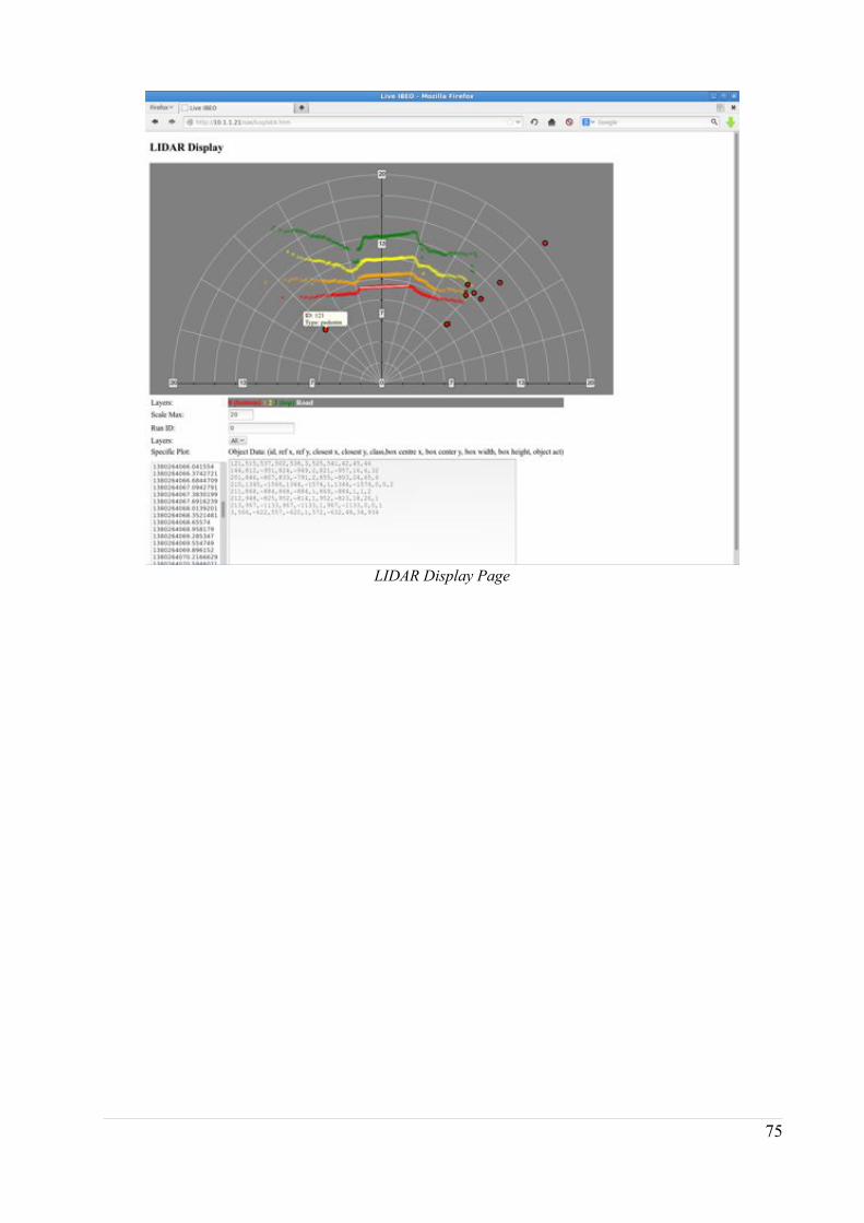
75

LIDAR Display Page

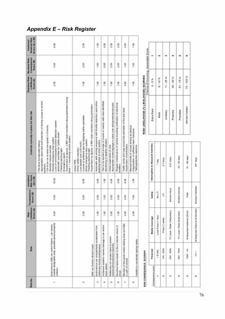
Appendix E – Risk Register

76

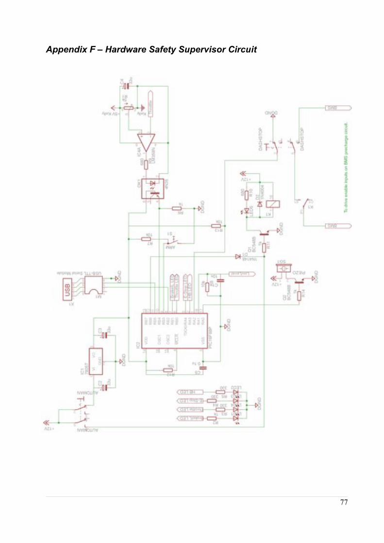
Appendix F – Hardware Safety Supervisor Circuit

77

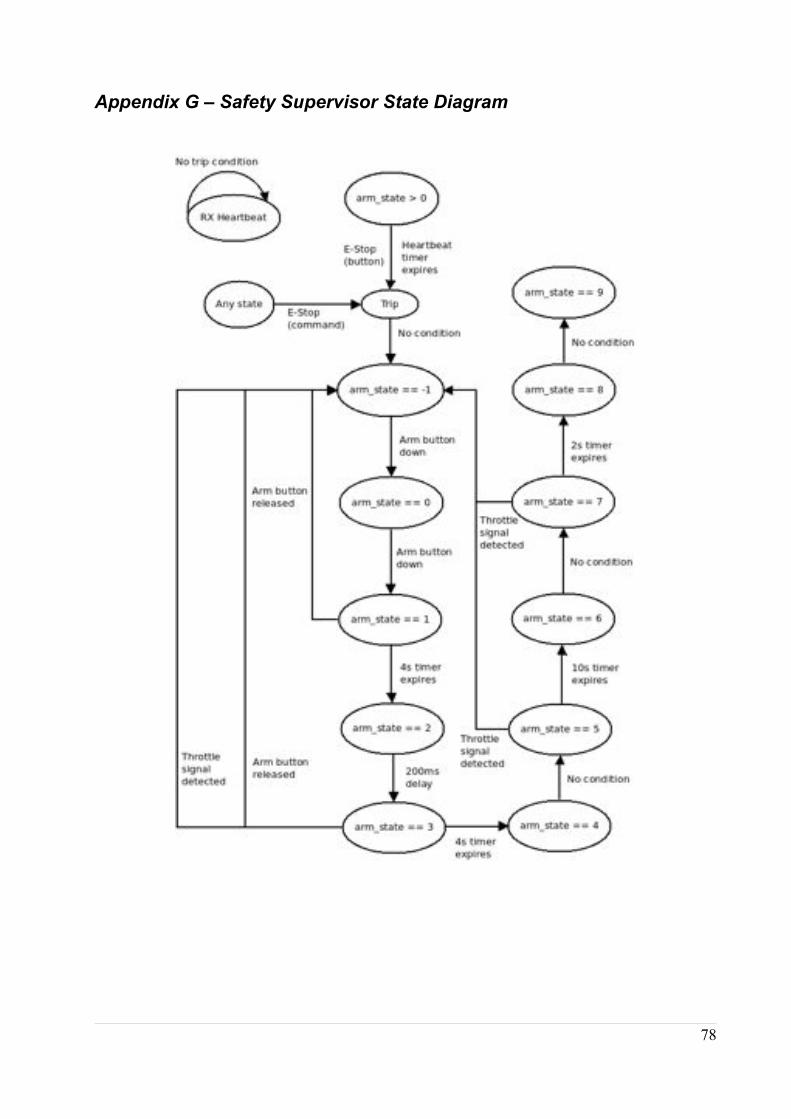
Appendix G – Safety Supervisor State Diagram

78

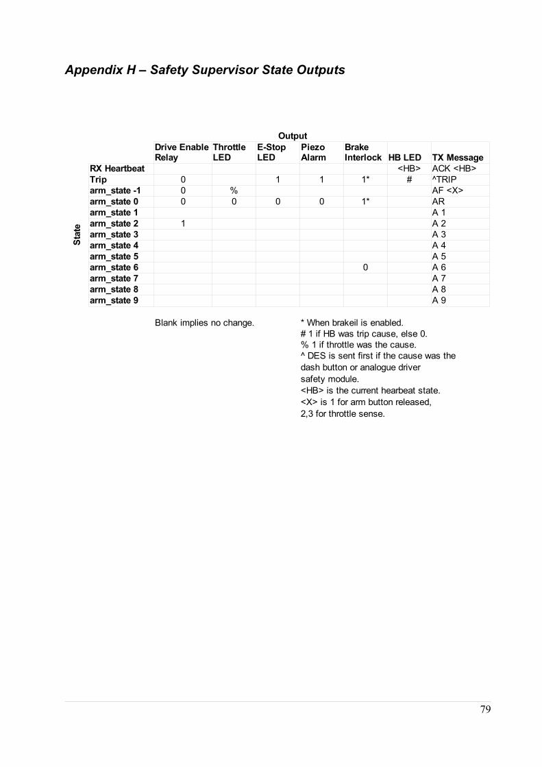
Appendix H – Safety Supervisor State Outputs

79

Output

HB LED TX Message

Sta

te

RX Heartbeat <HB> ACK <HB>

Trip 0 1 1 1* # ^TRIP

arm_state -1 0 % AF <X>

arm_state 0 0 0 0 0 1* AR

arm_state 1 A 1

arm_state 2 1 A 2

arm_state 3 A 3

arm_state 4 A 4

arm_state 5 A 5

arm_state 6 0 A 6

arm_state 7 A 7

arm_state 8 A 8

arm_state 9 A 9

Blank implies no change. * When brakeil is enabled.

# 1 if HB was trip cause, else 0.

% 1 if throttle was the cause.

^ DES is sent first if the cause was the

dash button or analogue driver

safety module.

<HB> is the current hearbeat state.

<X> is 1 for arm button released,

2,3 for throttle sense.

Drive Enable Relay

Throttle LED

E-Stop LED

Piezo Alarm

Brake Interlock