Embed Size (px)
Citation preview
Development and Application of Statistical Methods to
Support Air Quality Policy Decisions
José Carlos Magalhães Pires
Graduated in Chemical Engineering by the Faculty of Engineering of the University of Porto
Dissertation submitted to obtain the degree of
Doctor of Philosophy in Environmental Engineering
Porto, July 2009

Development and Application of Statistical Methods to
Support Air Quality Policy Decisions
José Carlos Magalhães Pires
Supervision
Fernando Gomes Martins (PhD) and Maria do Carmo da Silva Pereira (PhD) Department of Chemical Engineering, Faculty of Engineering, University of Porto
Porto, July 2009

V
Abstract
It is well known the health effects associated with air pollution. Several studies
were published, showing an increasing awareness among the scientific community
and policy makers about public health problems due to exposure to air pollution.
Policy makers require more detailed air quality information to take measures to
reduce the effects on health and to improve the air quality management. This
thesis aims to develop procedures using statistical methods to support a broad
range of policy decisions concerning this subject.
The first aim was the application of statistical methods, such as principal
component analysis and cluster analysis, to characterize the air pollution
behaviours in an urban area allowing the identification of monitoring sites with
redundant air quality measurements. These measurements represent a loss of
profitability of the air quality monitoring network resources. Accordingly, the
application of these statistical methods let the following policy decisions: (i)
remove the redundant monitoring sites, reducing the costs of the equipment
maintenance; or (ii) move the redundant monitoring sites to other places increasing
the area of monitored region. The air pollutant concentrations at the removed sites
can be estimated with statistical models using the concentrations measured at the
remaining sites. Moreover, the air pollution behaviours are related with the
location of emission sources. The possible location of important sources of air
pollutants was also determined through the analysis of variation of their
concentrations with the wind direction. Concerning the characterization of the air
pollution behaviours, the actual distribution of monitoring sites in the air quality
monitoring network of Oporto Metropolitan Area presented several redundant
measurements. The number of monitoring sites could be reduced at about 50% in
some of the analysed air pollutants. Several air pollution sources were identified
with the analysis of the variation of the air pollutant concentrations with the wind
VI
direction. The most important source was located at E-SE direction sector
affecting all monitoring sites during the analysed period.
The second aim of this thesis was the development of statistical models to predict
the concentrations of air pollutants (O3 and PM10) of the next day. Several models
were applied, including linear and non-linear ones. As far as the author knows,
independent component regression, partial least squares regression, stepwise
artificial neural networks, threshold regression and genetic programming were
applied for the first time in this field. Besides prediction of the air pollutant
concentrations, these models selected the important variables (environmental and
meteorological) that influence these values, which is an useful information for the
air quality management. The linear models had an advantage of taking less
computational time than the other models. Taking into account the performance of
these models, quantile regression presented better results in the training period, as
it tries to model the entire distribution of the dependent variable. However, this
model presented worse performance in the test period. The linear model with best
predictive performance was the partial least squares regression. Despite having
longer computation time, the non-linear models predicted better than the linear
ones, specially the models using the evolutionary procedure for their
determination. Threshold regression using genetic algorithms and genetic
programming for O3 and multi-gene genetic programming for PM10 were the
models with better predictive performance.
Keywords: air quality management, statistical methods, air quality modelling,
linear models, artificial neural networks, genetic programming.
VII
Resumo
Os efeitos negativos associados à poluição do ar são bem conhecidos. Muitos
estudos foram publicados, apresentando uma crescente preocupação da
comunidade científica e dos decisores políticos relativamente aos problemas de
saúde pública causados pela poluição do ar. Os decisores políticos necessitam de
informação mais detalhada sobre a qualidade do ar de modo a tomar medidas de
redução dos seus efeitos na saúde e melhorar a gestão da qualidade do ar. Este
trabalho tem como principal objectivo o desenvolvimento de procedimentos
usando métodos estatísticos para apoio de decisões políticas relacionadas com este
tema.
A aplicação de métodos estatísticos, tais como a análise de componentes principais
e análise de agrupamentos, permitiu a caracterização da variação da concentração
dos poluentes atmosféricos numa região urbana e, ao mesmo tempo, a
identificação de locais de monitorização com medições redundantes. Estas
medições representam uma perda de rentabilidade dos recursos das redes de
monitorização da qualidade do ar. Deste modo, a aplicação dos referidos métodos
estatísticos pode suportar as seguintes decisões: (i) eliminar as estações de
monitorização com medições redundantes, reduzindo os custos relativos à
manutenção do respectivo equipamento; ou (ii) deslocalizar as referidas estações
para outros locais, aumentando a área da região monitorizada. As concentrações de
poluentes nos locais em que se pode desactivar as estações podem ser estimadas
com modelos estatísticos usando os valores medidos nas restantes estações de
monitorização. A variação das concentrações dos poluentes atmosféricos está
relacionada com a localização relativa de fontes de emissão dos respectivos
poluentes. A possível localização de importantes fontes de emissão foi
determinada através da análise da variação da concentração de poluentes com a
direcção do vento. Caracterizando as variações observadas pelas concentrações
dos poluentes analisados, verificou-se que a distribuição das estações na rede de
VIII
monitorização da Área Metropolitana do Porto apresentava várias medições
redundantes. O número de locais de monitorização pode, para alguns poluentes,
ser reduzido para metade. Várias fontes de emissão foram identificadas com a
análise da variação da concentração de poluentes com a direcção do vento. A mais
importante esteve localizada fora da região definida pela rede de monitorização na
direcção E-SE, afectando todas as estações durante o período analisado.
Vários modelos estatísticos (lineares e não lineares) foram desenvolvidos para
prever as concentrações dos poluentes atmosféricos (O3 e PM10). Tanto quanto se
sabe, a regressão por componentes independentes, a regressão por mínimos
quadrados parciais, as redes neuronais artificiais desenvolvidas passo a passo, a
regressão com limiares e a programação genética foram técnicas de modelização
aplicadas pela primeira vez nesta área. Além de prever as concentrações de
poluentes atmosféricos, estes modelos seleccionam variáveis importantes
(concentrações de outros poluentes ou variáveis meteorológicas) que influenciam
esses valores, sendo uma informação útil para a gestão da qualidade do ar. Os
modelos lineares têm a vantagem de necessitar de menos tempo de computação do
que os modelos não lineares. Tendo em conta os desempenhos destes modelos, a
regressão por percentis teve melhores resultados no período de treino, uma vez que
o modelo tenta descrever toda a distribuição da variável dependente. No entanto,
este modelo teve pior desempenho na etapa de previsão. O modelo linear com
melhor desempenho na previsão foi a regressão por mínimos quadrados parciais.
Apesar de ter maior tempo de computação, os modelos não lineares prevêem
melhor que os modelos lineares, especialmente quando usam o procedimento
evolucionário na sua determinação. Assim, os modelos com limiares usando
algoritmos genéticos e programação genética para o O3 e programação genética
com múltiplos genes para PM10 foram os que apresentaram os melhores
desempenhos.
Palavras-chave: qualidade do ar, métodos estatísticos, modelização da qualidade
do ar, modelos lineares, redes neuronais artificiais, programação genética.
IX
Résumé
Les effets négatifs associés à la pollution de l’air sont bien connus. Plusieurs
études ont été publiées montrant la préoccupation croissante de la communauté
scientifique et des décideurs politiques concernant les problèmes de santé publique
causés par la pollution de l’air. Les décideurs politiques ont la nécessité d’avoir
une information plus détaillée de la qualité de l’air afin de pouvoir prendre des
mesures de réduction de ces effets sur la santé et améliorer la gestion de la qualité
de l’air. Ce travail a pour principal objectif le développement de procédures
utilisant des méthodes statistiques de forme a soutenir les décisions politiques liées
à ce sujet.
L’application de méthodes statistiques, telles que l’analyse en composantes
principales et l’analyse de grappes, a permis la caractérisation de la variation de la
concentration des polluants atmosphériques dans une zones urbaines ainsi que
l’identification de sites de surveillance avec des mesures redondantes. Ces mesures
représentent une perte de rentabilité des ressources des réseaux de surveillance de
la qualité de l’air. Ainsi, l’application de ces methodes statistiques peuvent
appuyer les decisions politiques suivantes: (i) éliminer les sations de surveillance
avec des mesures redondantes, reduisant le coût d’entretien des equipements; ou
(ii) déplacer ces stations à d’autres endroits, augmentant l’aire de la region
controlée. Les concentrations de polluants dans les endroits oú l’on peut désactiver
les sations peuvent être estimés à l’aide de modèles statistiques utilisant les valeurs
moyennes mesurées dans les autres sations de surveillance. La variation des
concentrations des polluants atmosphériques est liée à la localisation relative des
sources d’émission des polluents respectifs. Le possible emplacement de sources
importantes de polluants a également éte déterminé par l’analyse de la variation de
leurs concentrations avec la direction du vent. À travers la caractérisation des
variations observées par les concentrations de polluants analysés, il a été constaté
que la distribution des sites dans les réseau de surveillance de la zone

X
métropolitaine de Porto présentait plusieurs mesures redondantes. Le nombre de
sites de surveillance peut, pour certains polluants, être réduit de moitié. Plusieurs
sources d’émissions ont été identifiés à travers l’analyse de la variation de la
concentraction de polluants avec la direction du vent. La plus importante était
située à l’extérieur de la region définie par le réseau de surveillance dans la
direction E-SE, affectant l’ensemble des stations au cours de la période analysée.
Plusieurs modèles statistiques, linéaires et non linéaires, ont été développés afin de
prévoir les concentrations de polluants atmosphériques (O3 e PM10). Pour autant
qu’il se sache, la régression par composants indépendants, la régression des
moindres carrés partiels, les réseaux neuronaux artificiels développés pas à pas, la
régression avec des seuils et la programmation génétique ont été des techniques de
modélisation appliquées pour la première fois dans ce domaine. En plus de pévoir
les concentrations de polluants atmosphériques, ces modèles sélectionnent des
variables importantes qui influent sur ces valeurs, étant ainsi une information utile
pour la gestion de la qualité de l’air. Les modèles linéaires ont l’avantage d’exiger
moins de temps de calcul que les modèles non linéaires. Compte tenu de la
performance de ces modèles, la régression quantile a présenté de meilleurs
résultats au cours de la période d’essai, une fois que le modèle tente de décrire
l’ensemble de la distribution de la variable dépendante. Toutefois, ce modèles
présente une pire performance prédictive. Le modèle linéaire ayant la meilleure
performance en matière de prévision est la régression des moindres carrés partiels.
Bien qu’ayant un temps de calcul superieur, les modèles non linéaires prédisent
mieux que les modéles linéaires, en particulier ceux utilisant le processus
d’évolution dans sa détermination. Ainsi, les modèles avec des seuils utilisant des
algorithmes génétiques et la programmation génétique pour le O3 et la
programmation génétiques avec multiples genes pour PM10 ont été ceux présentant
les meilleures performances.
Mots-clés: qualité de l’air, méthodes statistiques, modélisation de la qualité de
l’air, modèles linéaires, réseaux de neurones artificiels, programmation génétique.

XI
Acknowledgements
I am grateful to my supervisors Fernando Gomes Martins (PhD) and Maria do
Carmo da Silva Pereira (PhD), for introducing me this research topic and then
providing me the necessary support. I also wish to thank Maria da Conceição
Machado Alvim Ferraz (PhD) for her advice, suggestions and for sharing her
knowledge in air quality with me. I can not forget the important suggestions and
contributions of Joana, Sofia and Elodie in the preparation of this manuscript.
I also acknowledge: (i) the Faculdade de Engenharia da Universidade do Porto,
the Departamento de Engenharia Química and Laboratório de Engenharia de
Processos, Ambiente e Energia for providing all the necessary facilities to perform
my studies; (ii) the Fundação para a Ciência e a Tecnologia for the fellowship
SFRH/BD/23302/2005; and (iii) the Comissão de Coordenação e
Desenvolvimento Regional do Norte and the Instituto Geofísico da Universidade
do Porto for kindly providing the air quality and meteorological data.
At the end, I want to thank my family, Nádia and my friends for the support,
patience and encouragement during this period.
To my family
To Nádia
To my friends

XIII
Table of Contents
Abstract ..................................................................................................................V
Resumo................................................................................................................VII
Résumé ................................................................................................................. IX
Acknowledgements.............................................................................................. XI
Table of Contents .............................................................................................XIII
Figure Index...................................................................................................... XVI
Table Index ....................................................................................................... XIX
List of Abbreviations..................................................................................... XXIII
Notation.......................................................................................................... XXVI
1. Introduction ...................................................................................................1
1.1. Scientific relevance.................................................................................1
1.2. Thesis structure .......................................................................................2
Part I. Management of Air Quality Monitoring Networ ks
2. Air Quality Evaluation in Oporto Metropolitan Area . ..............................7
2.1. Sulphur dioxide.......................................................................................7
2.2. Particulate matter ....................................................................................9
2.3. Carbon monoxide....................................................................................9
2.4. Nitrogen oxides.....................................................................................10
2.5. Ozone....................................................................................................11
2.6. Air quality data .....................................................................................13
2.7. Exceedances to EU limits .....................................................................14
2.8. Conclusions...........................................................................................21
3. Characterization of Air Pollution Behaviours ..........................................23
3.1. Introduction...........................................................................................23
3.2. Air quality data .....................................................................................25
3.3. Results and discussion ..........................................................................25
3.4. Conclusions...........................................................................................47
XIV
4. Identification of redundant air quality measurements............................ 49
4.1. Introduction.......................................................................................... 49
4.2. Air quality data..................................................................................... 50
4.3. Results and discussion.......................................................................... 51
4.4. Conclusions.......................................................................................... 57
Part II. Prediction of Air Pollutant Concentrations
5. Prediction using statistical models ............................................................ 63
5.1. State of the art ...................................................................................... 63
5.2. Models applied in this thesis ................................................................ 66
6. Linear models.............................................................................................. 67
6.1. Multiple linear regression .................................................................... 67
6.2. Principal component regression ........................................................... 69
6.3. Independent component regression...................................................... 71
6.4. Partial least squares regression............................................................. 72
6.5. Quantile regression............................................................................... 73
6.6. Statistical significance of regression parameters ................................. 74
6.7. Performance indexes ............................................................................ 75
6.8. Data ...................................................................................................... 76
6.9. Results and discussion.......................................................................... 77
6.10. Conclusions.......................................................................................... 83
7. Stepwise artificial neural networks ........................................................... 85
7.1. Introduction.......................................................................................... 85
7.2. Stepwise artificial neural networks ...................................................... 88
7.3. Data ...................................................................................................... 92
7.4. Results and discussion.......................................................................... 93
7.5. Conclusions.......................................................................................... 97
8. Threshold regression models ..................................................................... 99
8.1. Introduction.......................................................................................... 99
8.2. Genetic algorithms and TR-GA procedure ........................................ 100
8.3. Data .................................................................................................... 103

XV
8.4. Results and discussion ........................................................................104
8.5. Conclusions.........................................................................................106
9. Genetic Programming ...............................................................................109
9.1. Introduction.........................................................................................109
9.2. Genetic programming .........................................................................110
9.3. Data.....................................................................................................114
9.4. Results and discussion ........................................................................115
9.5. Conclusions.........................................................................................119
10. Multi-gene Genetic Programming .......................................................121
10.1. Introduction.........................................................................................121
10.2. Data.....................................................................................................122
10.3. Results and discussion ........................................................................123
10.4. Conclusions.........................................................................................128
11. Final Words ...........................................................................................129
11.1. General conclusions............................................................................129
11.2. Future work.........................................................................................132
References ...........................................................................................................133
XVI
Figure Index
Figure 2.1 Location of the monitoring sites in the map of Oporto-MA (from Google Earth). ....................................................................................................... 15
Figure 3.1 Dendrograms resulting from the application of CA to the (a) SO2, (b) PM10, (c) CO, (d) NO2 and (e) O3 concentrations............................................ 28
Figure 3.2 Average daily profile of the hourly average SO2 concentrations at the monitoring sites grouped by the correspondent PC/CL category: (a) PC1/CL1, (b) PC2/CL3, (c) PC3/CL5, (d) PC4/CL2, (e) PC5/CL4 and (f) PC6/CL6................................................................................................................ 30
Figure 3.3 Average daily profile of the hourly average PM10 concentrations for the monitoring sites grouped by the correspondent PC/CL category: (a) PC1/CL2 and (b) PC2/CL1. .................................................................................. 31
Figure 3.4 Average daily profile of the hourly mean CO concentrations for the monitoring sites grouped by the correspondent PC/CL category: (a) PC1/CL1, (b) PC2/CL3, and (c) PC3/CL2. ............................................................................ 32
Figure 3.5 Average daily profile of the hourly average NO2 concentrations for the monitoring sites grouped by the correspondent PC/CL category: (a) PC1/CL1, (b) PC2/CL2, and (c) PC1/CL3. ........................................................... 33
Figure 3.6 Average daily profile of the hourly average O3 concentrations for the monitoring sites grouped by the correspondent PC/CL category: (a) PC1/CL1 and (b) PC2/CL2.................................................................................................... 34
Figure 3.7 Relative frequency (%) of the direction from which the wind was blowing when hourly average concentrations of SO2 above 125 µg m-3 were collected (number of occurrences in brackets). ..................................................... 36
Figure 3.8 Relative frequency (%) of the direction from which the wind was blowing when hourly average concentrations of PM10 increased at least 50 µg m-3 during the period that lasted from 17 to the 22 hours (number of occurrences in brackets). ....................................................................................... 37
Figure 3.9 Example of the profile of the hourly average PM10 concentrations when the wind blew predominantly from S-SW direction sector. .................................. 39
XVII
Figure 3.10 Relative frequency (%) of the direction from which the wind was blowing when hourly average CO concentration above 4 mg m-3 was collected (number of occurrences in brackets). .....................................................................40
Figure 3.11 Examples of the daily profiles of CO concentrations when the wind blew predominantly from: (a) NE-E, and (b) NW-N direction sectors. .................41
Figure 3.12 Relative frequency (%) of the direction from which the wind was blowing when hourly average NO2 concentration above 100 µg m-3 was collected (number of occurrences in brackets).......................................................42
Figure 3.13 Example of the daily profile of NO2 concentrations when the wind blew predominantly from NW-N direction sector..................................................43
Figure 3.14 Relative frequency (%) of the direction from which the wind was blowing when hourly average O3 concentration above 120 µg m-3 was collected (number of occurrences in brackets). .....................................................................44
Figure 3.15 Example of the daily profile of O3 concentrations when the wind blew predominantly from W-NW direction sector.................................................45
Figure 3.16 Example of the daily profile of NO2 concentrations...........................46
Figure 4.1 Performance indexes of all MLR models in the (a) training and (b) test periods for the Kaiser criterion. .......................................................................58
Figure 4.2 Performance indexes of all MLR models in the (a) training and (b) test periods for the ODV90 criterion. ......................................................................59
Figure 7.1 Example of the first three steps of SWANN1 methodology (a-c) and its final result (d) for the case of three input neurons.............................................90
Figure 7.2 Example of the result of five steps of SWANN2 methodology (a-e) and its final result (f) for the case of three input neurons.......................................91
Figure 7.3 Variation of AIC value in the training set with the increase of the number of IHL synapses in SWANN2 models using OVs as inputs and the activation function sine. .........................................................................................93
Figure 7.4 SWANN2 model using OVs as inputs and the activation function sine. ........................................................................................................................94
Figure 7.5 Example of the predictions of: (a) O3 concentrations (with PCs and sine function); and (b) PM10 concentrations (with PCs and sigmoid function)......98
XVIII
Figure 8.1 Codification of chromosomes. ........................................................... 101
Figure 8.2 Procedure to apply GA for defining threshold regression models. .... 103
Figure 9.1 Example of tree representation of expressions used in GP and respective formula. .............................................................................................. 111
Figure 9.2 Example of crossover operation between two trees. .......................... 112
Figure 9.3 Examples of mutation operation in: (a) a function; and (b) a terminal................................................................................................................ 113
Figure 9.4 GP procedure...................................................................................... 114
Figure 9.5 Occurrence (in percentage) of each input for the 4 GP runs in the 20 best solutions of the last generation using 3, 4 and 5 populations (P3, P4 and P5): (a) OV and (b) PC........................................................................................ 117
Figure 9.6 Box and whisker diagrams with the performance indexes of GP models in training (a and b) and test (c and d) periods........................................ 118
Figure 9.7 Performance of the best GP model in all test period.......................... 119
Figure 10.1 Occurrence of each input for the 10 MGP runs in the best solutions (10 individuals) and in the 20 best solutions of the last generation (200 individuals). ......................................................................................................... 124
Figure 10.2 Performance of the MGP model in the test period........................... 127
XIX
Table Index
Table 2.1 Site characteristics of the air quality monitoring network of Oporto Metropolitan Area ..................................................................................................15
Table 2.2 Air pollutants whose concentrations are measured at each monitoring site ..........................................................................................................................16
Table 2.3 Annual averages of SO2 concentrations at each site (it should not exceed 20 µg m-3 for ecosystem protection) and the correspondent PAD (in brackets) .................................................................................................................17
Table 2.4 Number of exceedances of the limit established by the European Union for the protection of human health regarding daily averages of PM10
concentrations and the correspondent PAD (in brackets) ......................................18
Table 2.5 Annual averages of PM10 concentrations at each site (it should not exceed 40 µg m-3 for the protection of human health) and the correspondent PAD (in brackets)...................................................................................................18
Table 2.6 Annual average NO2 concentrations at each site (it should not exceed 40 µg m-3 for the protection of human health) and the correspondent PAD (in brackets) .................................................................................................................19
Table 2.7 Annual average NOx concentrations at each site (it should not exceed 30 µg m-3 for the protection of vegetation) and the correspondent PAD (in brackets) .................................................................................................................19
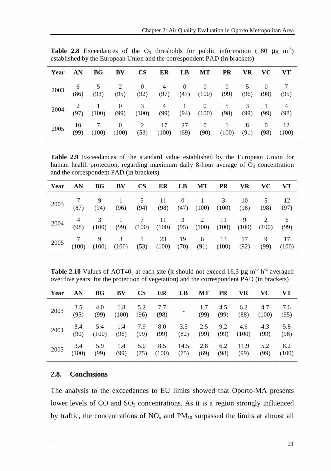
Table 2.8 Exceedances of the O3 thresholds for public information (180 µg m-3) established by the European Union and the correspondent PAD (in brackets)......21
Table 2.9 Exceedances of the standard value established by the European Union for human health protection, regarding maximum daily 8-hour average of O3 concentration and the correspondent PAD (in brackets) ..............................21
Table 2.10 Values of AOT40v at each site (it should not exceed 16.3 µg m-3 h-2 averaged over five years, for the protection of vegetation) and the correspondent PAD (in brackets) ...........................................................................21
Table 3.1 Main results of the PCA application for the analysed pollutants at all sites.........................................................................................................................26
XX
Table 4.1 Main results of the PCA application for O3 at all monitoring sites during the third quarter of 2004............................................................................. 52
Table 4.2 Number of PCs selected for each analysed period using the two criteria: Kaiser (left) and ODV90 criterion (right).................................................. 53
Table 4.3 Relative frequency (in percentage) of each pair of monitoring sites with important contributions in the same PC during the first two years of study (eight periods) using Kaiser criterion (upper triangular matrix) and ODV90 criterion (lower triangular matrix)......................................................................... 55
Table 4.4 MLR models used to estimate the air pollutant concentrations at all removed monitoring sites using the values measured at other sites in Oporto-MA for the Kaiser criterion ................................................................................... 56
Table 4.5 MLR models used to estimate the air pollutant concentrations at all removed monitoring sites using the values measured at other sites in Oporto-MA for ODV90 criterion ........................................................................................ 56
Table 6.1 Regression parameters for all statistical models for O3 concentrations prediction............................................................................................................... 78
Table 6.2 Regression parameters for all statistical models for PM10 concentrations prediction....................................................................................... 79
Table 6.3 Varimax rotated factor loadings ............................................................ 79
Table 6.4 Correlation matrix between the original variables and the IC for O3 and PM10................................................................................................................ 80
Table 6.5 Performance indexes of the different statistical models for the training period ....................................................................................................... 82
Table 6.6 Performance indexes of the different statistical models for the test period..................................................................................................................... 82
Table 7.1 Number of IHL synapses, hidden neurons and parameters presented by SWANN1 and SWANN2 models obtained for the different activation functions and type of input variables..................................................................... 95
Table 7.2 Performance indexes of the SWANN1 and SWANN2 models in the training set for predicting O3 and PM10 concentrations......................................... 95
Table 7.3 Performance indexes of the SWANN1 and SWANN2 models in the validation set for predicting O3 and PM10 concentrations ..................................... 96
XXI
Table 7.4 Performance indexes of the SWANN1 and SWANN2 models in the test set for predicting O3 and PM10 concentrations.................................................96
Table 8.1 Statistically significant regression parameters for TR-GA (M1 to M6) and MLR models and correspondent RMSE value in the training data ...............105
Table 8.2 Performance indexes of the TR-GA and MLR models in the test period....................................................................................................................105
Table 9.1 Values of GP control parameters..........................................................115
Table 9.2 Principal components varimax rotated loadings ..................................116
Table 10.1 Best solutions of the 10 MGP runs and correspondent RMSE in the training period ......................................................................................................125
Table 10.2 Performance indexes of the best solutions of the 10 MGP runs in the test period .............................................................................................................126


XXIII
List of Abbreviations
AIC Akaike Information Criterion
AN Antas
ANN Artificial neural network
AOT40 Accumulated exposure over a threshold of 40 ppb
AOT40v Averaged exposure Over a Threshold of 40 ppb
AQMN Air quality monitoring network
BG Baguim
BV Boavista
CA Cluster analysis
CL Cluster
CS Custóias
E East
EC European Council
ER Ermesinde
EU European Union
GA Genetic algorithm
GP Genetic programming
HOL Hidden-to-output layer
IC Independent component
ICA Independent component analysis
ICi Independent component i
ICR Independent component regression
IHL Input-to-hidden layer
k-NN k-nearest neighbours
LB Leça do Balio
MAE Mean absolute error
MBE Mean bias error
XXIV
MGP Multi-gene genetic programming
MLR Multiple linear regression
MT Matosinhos
N North
NE Northeast
NW Northwest
ODV90 90% of the original data variance
Oporto-MA Oporto Metropolitan Area
OV Original variable
PAD Percentage of available data
PC Principal component
PCA Principal component analysis
PCi ith principal component
PCR Principal component regression
PLSR Partial least squares regression
PM Particulate matter
PR Perafita
Qi ith annual quarter
QR Quantile regression
RH Relative humidity
RMSE Root mean squared error
S South
SE Southeast
SH Senhora da Hora
sig Sigmoid function
sin Sine function
SR Solar radiation
SSE Sum of the squared errors
SW Southwest

XXV
SWANN Stepwise artificial neural network
T Air temperature
tgh Hyperbolic tangent function
TR Threshold regression
USEPA United States Environmental Protection Agency
UV Ultraviolet
VC Vila do Conde
VOC Volatile Organic Compounds
VR Vermoim
VT Vila Nova da Telha
W West
WBG World Bank Group
WHO World Health Organization
WS Wind speed
XXVI
Notation
α Significance level
iα Regression parameters
iβ Regression parameters
iν Regression parameters
ε Error associated with the regression
λ Eigenvalue
θ Bias
σ Standard deviation
σ2 Variance
τ Percentile
(X)-1 Inverse of the matrix X
(X)T Transpose of the matrix X
|X| Determinant of the matrix X
B Regression parameters matrix
b Regression parameters vector
bjp Loading of the original variable j in the principal component p
BPLS Regression parameters of partial least squares regression
c y weight vector
C y weights matrix
Cov Covariance matrix
CO Carbon monoxide
d Index of threshold variable
d2 Index of agreement of second order
F() Cumulative probability density function

XXVII
f() Activation function
I Identity matrix
k Number of parameters
n Number of data points
NO Nitrogen oxide
NO2 Nitrogen dioxide
NOx Nitrogen oxides
O3 Tropospheric ozone
O3|t+24h Next day hourly average ozone concentrations
P X loadings matrix
p X loadings vector
PM10 Particulate matter with aerodynamic diameter smaller than 10 µm
PM2.5 Particulate matter with aerodynamic diameter smaller than 2.5 µm
R Pearson correlation coefficient
r Threshold value
SO2 Sulphur dioxide
Sxxi Sum of squares related to xi
t Student t distribution
T X score matrix
t X score vector
U y score matrix
u y score vector
W X weight matrix
w X weight vector
wi Weight value
X Matrix of the explanatory variables
X0 X standardized matrix
xd Threshold variable
xi Input value

XXVIII
iY Output value
iY Model output
iY Average of the output variable
y Output value
y Vector of the dependent variable
y0 y standardized vector

1
Chapter 1
1. Introduction
This chapter describes the project associated with this thesis. The importance of this study is also demonstrated. At the end, there is a description of the structure of the thesis.
1.1. Scientific relevance
Clean air is considered to be a basic requirement of human health. The quality of
the air is the result of a complex interaction of many factors that involve the
chemistry and motions of the atmosphere, as well as the emissions of a variety of
pollutants from sources that are both natural and anthropogenic.
Before the increase of large cities and industries, the nature was able to keep the
air fairly clean. Wind mixed and dispersed the gases, rain washed the dust and
other easily dissolved substances to the ground and plants absorbed carbon dioxide
and replaced it by oxygen. With urbanisation and industrialisation, humans started
to release more wastes into the atmosphere than nature could manage with. Thus,
these concentrated gases exceed safe limits and became a pollution problem.
Air pollution can not be considered a local problem. The air pollutants released in
one country can be transported by the wind, causing several negative impacts (in
human health, vegetation, ecosystems, climate and materials) elsewhere. Thus, air
pollution should be considered as a transboundary concern.
Development and Application of Statistical Methods to Support Air Quality Policy Decisions
2
European Union established several directives related with air quality. These
directives established limit values for air pollutant concentrations concerning the
protection of the human health, vegetation and ecosystems. They also indicate the
number of monitoring sites that should operate according to population size and
pollution levels. However, the number and location of the monitoring sites should
be optimized for the different regions. In other words, the redundant measurements
should be avoided due to the high cost of the monitoring equipment maintenance.
One of the most important air pollutant usually associated with poor air quality is
tropospheric ozone (O3). O3 is naturally present in the atmosphere, but in elevated
amounts it is damaging to the living tissue of plants and animals. However, the
most relevant pollutant for air quality is particulate matter (PM). An important
target of this thesis is the prediction of concentrations of O3 and PM10 (particulate
matter with aerodynamic diameter smaller than 10 µm) with a day in advance.
Thus, the persons belonging to risk groups (with respiratory problems, children
and elderly) can be advised for high concentrations episodes. Other components
important in air quality include carbon monoxide, sulphur dioxide, NOx and VOC
(O3 precursors), and air toxics such as benzene, mercury and other hazardous air
pollutants.
The need for improved understanding of the science of air quality remains a
priority for the wider scientific and user communities. Despite improvements in
technology, users still require new, robust management and assessment tools to
formulate effective control policies and strategies for reducing the health impact of
air pollution. Accordingly, this thesis presents statistical methods useful for policy
makers seeking to improve air quality management in their cities.
1.2. Thesis structure
The project associated with this document, entitled Development and Application
of Statistical Methods to Support Air Quality Policy Decisions, was performed at
Chapter 1: Introduction
3
Departamento de Engenharia Química of Faculdade de Engenharia da
Universidade do Porto from 2006 to 2009.
The thesis was divided in two parts: (i) management of air quality monitoring
networks (Part I); and (ii) prediction of air pollutant concentrations (Part II). Part I
contains the Chapters 2 to 4, while Part II contains the Chapters 5 to 10.
Chapter 2 describes the air pollutants whose monitoring is of particular interest for
the characterization of the air quality. Their sources, effects and legislation related
with their concentrations are the main topics focused. Additionally, this chapter:
(i) characterizes the region where the air quality was measured; (ii) refers the
equipment used for each air pollutant monitoring; and (iii) determines for a
specific period the number of exceedances to the limits established by the EU for
protection of human health, vegetation and ecosystems.
Chapter 3 shows how principal component analysis and cluster analysis can be
applied to define the number of monitoring sites that should operate in an air
quality monitoring network (AQMN). Additionally, the location of the main
emission sources was identified based on the influence of wind direction on the
increase of the air pollutant concentrations.
In Chapter 4, principal component analysis was applied using another criterion to
select the number of principal components. This number, corresponding to the
minimum number of monitoring sites that should operate, was then compared with
the value presented by the European legislation. At the end of this chapter, the air
pollutant concentrations at the removed monitoring sites were estimated using the
values of the selected monitoring sites.
Chapter 5 presents several previous studies about prediction of O3 and PM10
concentrations through statistical models.
Chapter 6 shows the comparison of the performance of five linear models in the
prediction of O3 and PM10 concentrations.

Development and Application of Statistical Methods to Support Air Quality Policy Decisions
4
Chapter 7 presents two step-by-step methodologies to define artificial neural
network models. These models were applied to predict the concentrations of the
same air pollutants.
Chapter 8 shows how to apply genetic algorithms to define threshold regression
models for prediction of O3 concentrations.
In Chapter 9, genetic programming was applied to predict O3 concentrations.
In Chapter 10, multi-gene genetic programming was applied to predict PM10
concentrations.
Finally, Chapter 11 presented the main conclusions of this thesis and some
suggestions for future work.
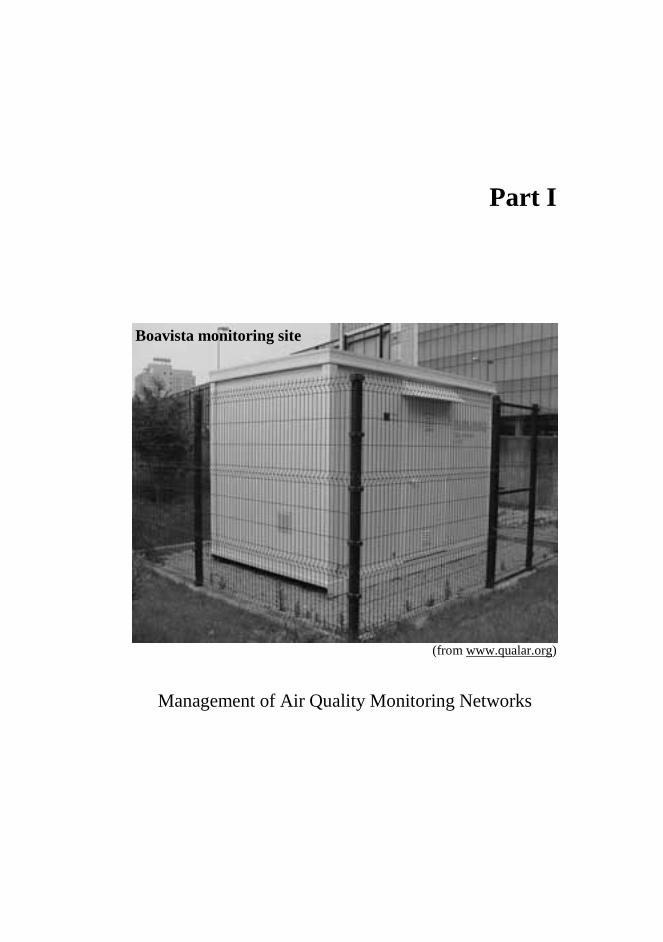
Part I
(from www.qualar.org)
Management of Air Quality Monitoring Networks
Boavista monitoring site

7
Chapter 2
2. Air Quality Evaluation in Oporto Metropolitan Area
This chapter describes the air pollutants whose monitoring is of particular interest for the characterization of the air quality. Their sources, effects and the legislation related with their concentrations are the main topics of this chapter. Additionally, the aims are: (i) characterize the region where the air quality was measured; (ii) refer to the equipment used for each air pollutant monitoring; and (iii) determine for this period the number of exceedances to the limits established by the European Union for protection of human health, vegetation and ecosystems.
The contents of this chapter were adapted from: (i) Pires, J.C.M., Sousa, S.I.V., Pereira, M.C., Alvim-Ferraz, M.C.M., Martins, F.G., 2008. Management of Air Quality Monitoring using Principal Component and Cluster Analysis – Part I: SO2 and PM10. Atmospheric Environment 42 (6), 1249-1260; and (ii) Pires, J.C.M., Sousa, S.I.V., Pereira, M.C., Alvim-Ferraz, M.C.M., Martins, F.G., 2008. Management of Air Quality Monitoring using Principal Component and Cluster Analysis – Part II: CO, NO2 and O3. Atmospheric Environment 42 (6), 1261-1274.
2.1. Sulphur dioxide
Sulphur dioxide (SO2) is one of the most important pollutants, as it results from
the combustion of sulphur compounds. Volcanoes and oceans are the major
natural sources of SO2 (Carmichael et al., 2002; Garg et al., 2006; Reddy and
Venkataraman, 2002; World Health Organization - WHO, 2000). Anthropogenic
emissions of SO2 come from the combustion of fossil fuels (mainly coal and heavy
oils), biomass burning and the smelting of sulphur containing ores.
Many efforts have been done to reduce SO2 emissions; consequently, in the last 20
years the atmospheric levels of SO2 have been continuously decreasing in most
Part I: Management of Air Quality Monitoring Networks
8
Western industrialized countries (Nunnari et al., 2004). SO2 and its oxidation by-
products are removed from the atmosphere by wet and dry deposition (acid
precipitation). Besides these transformation and removal processes, SO2 can be
carried out over large distances, causing transboundary pollution (ApSimon and
Warren, 1996).
SO2 is an irritant gas when inhaled and at high concentrations may cause breathing
difficulties in people directly exposed to it. Absorption of SO2 in the nose mucous
membranes and in the upper respiratory tract results from its solubility in water
(WHO, 2000). The effects of SO2 inhalation appear in only a few minutes and
people suffering from asthma and chronic lung disease may be especially
susceptible to its adverse effects. This pollutant also affects plants and depending
on its concentration levels, can produce: chlorophyll degradation; reduction of
photosynthesis; raise of respiration rates; and changes in protein metabolism
(Carlson, 1979; Lee et al., 1997). Nevertheless, sulphur is an important nutrient for
plants due to the fact that, by instance, atmospheric sulphur may be taken up by
leaves of some species, contributing to the plant vitality in soils with low sulphur
concentrations such as calcareous soils. SO2 (combined with other air pollutants
and under specific conditions of relative humidity, temperature and precipitation)
is responsible for the deterioration of materials, such as metals and stones. In many
parts of Europe, some monuments which resisted deterioration for hundreds or
even thousands of years have shown an accelerated degradation of their surface in
the last decades.
The European Union (EU) established limit values for SO2 concentrations: (i) the
hourly limit for the protection of human health (350 µg m-3, not to be exceeded
more than 24 times per year); (ii) the daily limit for the protection of human health
(125 µg m-3, not to be exceeded more than 3 times per year); and (iii) the annual
limit for protection of ecosystems (20 µg m-3) (EC Directive, 1999).
Chapter 2: Air Quality Evaluation in Oporto Metropolitan Area
9
2.2. Particulate matter
Particulate matter (PM) is the designation of solid and liquid particles suspended
in the atmosphere. They are emitted by both, natural (volcanic eruptions, seismic
activity and forest fires) and anthropogenic sources (all types of man-made
combustion and some industrial processes).
PM is one of the most important air pollutants that adversely influence human
health in Europe (Koelemeijer et al., 2006). In the last decade, several studies were
published about the impact of PM on human health (Alvim-Ferraz et al., 2005;
Brunekreef and Holgate, 2002; Dockery and Pope, 1994; Hoek et al., 2002). Long
exposure to PM10 and to PM2.5 (particles with an aerodynamic diameter smaller
than 10 and 2.5 µm, respectively) has been associated with respiratory and
cardiovascular diseases. Recent research seems to indicate that PM10 are
associated with childhood morbidity and mortality (Kappos et al., 2004).
Aiming the protection of human health, the EU established two limits for PM10,
which should be enforced on two different periods of time; the first beginning in
2005 and the last one in 2010. The limits to be enforced from 2005 until 2010 are:
(i) the daily limit of 50 µg m-3, not to be exceeded more than 35 times per year;
and (ii) the annual limit of 40 µg m-3. The limits to be enforced from 2010 are: (i)
the daily limit of 50 µg m-3, not to be exceeded more than 7 times per year; and (ii)
the annual limit of 20 µg m-3 (EC Directive, 1999).
2.3. Carbon monoxide
Carbon monoxide (CO) is a colourless, practically odourless, tasteless and no
irritating gas which is the result of the incomplete oxidation of carbon in
combustion (Raub, 1999; Raub et al., 2000). The main sources are the combustion
of fuel (that occurs when the ratio air-to-fuel presents low values), industrial
emissions and other combustion sources (as coal, gas, wood and kerosene).
Natural sources, such as volcanoes, natural gases in coal mines and forest fires,
have also an important contribution. The emissions of CO increase significantly

Part I: Management of Air Quality Monitoring Networks
10
during the cold weather. In these conditions, the engines need more fuel to work
and some emission control devices, such as oxygen sensors and catalytic
converters, operate less efficiently when they are cold (Raub et al., 2000; United
States Environmental Protection Agency - USEPA, 2004).
The effects in the human health associated to the presence of CO depend on its
concentration and the duration of exposure. At low concentrations, CO causes
fatigue in healthy people and chest pain in people with heart disease. At high
concentrations, it causes headaches, confusion and nausea. When inhaled, CO is
absorbed from the lungs to the bloodstream, where it forms a complex with
haemoglobin known carboxyhaemoglobin. The presence of this complex reduces
the oxygen carrying capacity, causing hypoxia (low oxygen level available to the
body tissues) (Raub, 1999; Raub et al., 2000; USEPA, 2000; USEPA, 2004;
WHO, 2000). CO is one of the contaminants found normally in the atmosphere
that requires prevention and control measures to ensure adequate protection of the
human health.
EU established 10 mg m-3 as a limit value for the protection of human health (EC
Directive, 2000) based in the maximum daily 8-hour average concentration.
2.4. Nitrogen oxides
Nitrogen oxides (NOx) are a group of highly reactive gases. These gases contain
atoms of nitrogen and oxygen in different proportions. Nitrogen oxide (NO) and
nitrogen dioxide (NO2) are the most important gases of this group and they are
considered significant pollutants in the troposphere (USEPA, 1998; World Bank
Group - WBG, 1998). Anthropogenic emissions of NOx result from the
combustion processes, including motor vehicles, electric utilities, and other
industrial, commercial and residential sources that burn fossil fuels. Natural
events, such as anaerobic biological processes in soil and water, volcanic activity
and photochemical destruction of nitrogen compounds in the upper atmosphere,
have also a high contribution for NOx emissions (USEPA, 1998; WBG, 1998).
Chapter 2: Air Quality Evaluation in Oporto Metropolitan Area
11
Nitrogen oxides have diverse negative effects (Hashim et al., 2004; Kalabokas et
al., 2002; USEPA, 1998; WBG, 1998; WHO, 2000), such as: (i) formation of acid
rain – they react with other substances in the air to form acids which fall to earth
as rain, fog, snow, or dry particles; (ii) deterioration of the water quality -
increased nitrogen loading in water bodies, particularly coastal estuaries, upsets
the chemical balance of nutrients used by aquatic plants and animals; (iii)
formation of toxic chemicals – NOx reacts with common organic chemicals to
form a wide variety of toxic products, such as nitrate radicals, nitroarenes and
nitrosamines; (iv) reduction of the visibility – nitrogen dioxide can block the
transmission of light; (v) contribution to the increase of the earth’s temperature –
one of the nitrogen oxides, nitrous oxide, is a greenhouse gas; and (vi) formation
of ground-level ozone – in the presence of hydrocarbons and sunlight, NOx
contribute to the formation of tropospheric ozone, which can cause serious
respiratory problems.
EU established limit values for NO2 and NOx (EC Directive, 1999). Concerning
hourly average concentrations, NO2 limit for the protection of human health is 200
µg m-3 and may not be exceed more than 18 times in the year (limit value to be
met till January of 2010). Concerning annual average concentrations, NO2 limit for
the protection of human health is 40 µg m-3 (limit value to be met till January of
2010) and NOx limit for protection of the vegetation is 30 µg m-3.
2.5. Ozone
Ozone (O3) is a strong photochemical oxidant found in the troposphere and in
other layers of the atmosphere. While ozone has an important role in the
stratosphere (protection from the ultraviolet radiation), in the troposphere this
irritating and reactive molecule has negative impacts on human health, climate,
vegetation and materials (Alvim-Ferraz et al., 2006; Chan et al., 1998).
Concerning human health effects, the most important are: (i) damage to respiratory
tract tissues; (ii) death of lung cells and increased rates of cell replication
Part I: Management of Air Quality Monitoring Networks
12
(hyperplasia); (iii) inflammation of airways; and (iv) increase of the respiratory
symptoms, such as cough, chest soreness, difficulty in taking a deep breath and, in
some cases, headaches or nausea (Kley et al., 1999; Leeuw, 2000). Concerning
climate, a temperature increase is expected to be related to the tropospheric ozone
increase, because it is a greenhouse gas and influences the atmospheric residence
time of other greenhouse gases (Bytnerowicz et al., 2006). In vegetation, it causes
leaf injury, growth and yield reduction, and changes in the sensitivity to biotic and
abiotic stresses (Alvim-Ferraz et al., 2006; Leeuw, 2000). Concerning materials,
ozone in combination with other atmosphere pollutants contributes to the increase
of the corrosion on building materials like steel, zinc, copper, aluminium and
bronze (Leeuw, 2000).
The presence of ozone in the troposphere is a result of three basic processes: (i)
photochemical production by the interaction of hydrocarbons and nitrogen oxides
(emitted by gasoline vapours, fossil fuel power plants, refineries, and other
industries) under the action of suitable ambient meteorological conditions (Guerra
et al., 2004; Strand and Hov, 1996; Zolghadri et al., 2004); (ii)
tropospheric/stratospheric exchange that causes the transport of stratospheric air,
rich in ozone, into the troposphere (Dueñas et al., 2002); and (iii) horizontal
transport due to the wind that brings ozone produced in other regions.
EU established limit values for ozone in the ambient air (EC Directive, 2002). The
information threshold (considered to carry health risks for short-time exposure of
groups particularly sensible) is 180 µg m-3 for hourly average concentration, and
the alert threshold (considered to carry health risks for short-time exposure of the
population in general) is 240 µg m-3. The O3 target value for the protection of the
human health is 120 µg m-3 concerning maximum daily 8-hour average
concentrations and may not be exceeded more than 25 days per calendar year
averaged over three years (limit value to be met till 2010). Concerning the
cumulative ozone exposure index (AOT40 – Accumulated exposure Over a
Threshold of 40 ppb or 80 µg m-3) calculated from 1 h values from May to July,
Chapter 2: Air Quality Evaluation in Oporto Metropolitan Area
13
the O3 target value for the protection of the vegetation is 18000 µg m-3 h-1 averaged
over five years (limit value to be met till 2010). The long-term objectives for O3 in
Europe are: (i) maximum daily 8-hour average of 120 µg m-3 for the protection of
the human health; and (ii) AOT40 calculated from 1 h values from May to July of
6000 µg m-3 h-1.
2.6. Air quality data
Oporto is the second largest city of Portugal, located at North. The important air
pollution sources in Oporto Metropolitan Area (Oporto-MA) are vehicle traffic, an
oil refinery, a petrochemical complex, a thermoelectric plant (planned for working
with natural gas), an incineration unit and an international shipping port (Pereira et
al., 2007).
The air quality data was collected from the monitoring sites integrated in the air
quality monitoring network (AQMN) of Oporto-MA, managed by the Regional
Commission of Coordination and Development of Northern Portugal (Comissão
de Coordenação e Desenvolvimento Regional do Norte), under the responsibility
of the Ministry of Environment. The AQMN of Oporto-MA is currently composed
of 14 monitoring sites that regularly monitor the air levels of SO2, PM10, CO, NO,
NO2, NOx and O3. PM2.5, benzene, toluene and xylene are also measured in some
monitoring sites of the network.
SO2 concentrations were obtained by the ultraviolet fluorescence method,
according to the EC Directive 1999/30/EC (EC Directive, 1999) using the AF21M
equipment from Environment SA (Pereira et al., 2007). PM10 concentrations were
obtained through the beta radiation attenuation method, considered equivalent to
the method advised by the EU Directive 1999/30/EC (EC Directive, 1999), using
the MPSI 100 I et E equipment from Environment SA (Pereira et al., 2005).
Nondispersive infrared spectrometric method was applied to measure the CO
concentrations (Sousa et al., 2006), according to the EU Directive 2000/69/EC
(EC Directive, 2000). NO2 and NOx were obtained through the chemiluminescence
Part I: Management of Air Quality Monitoring Networks
14
method (Sousa et al., 2006), according to EU Directive 1999/30/EC (EC Directive,
1999). Ozone measurements, according to EU Directive 2002/3/EC (EC Directive,
2002), were performed through UV-absorption photometry using the equipment
41 M UV Photometric Ozone Analyser from Environment S.A. (Pereira et al.,
2005). This equipment was submitted to a rigid maintenance program, being
calibrated each 4 weeks. Measurements were continuously registered and hourly
average concentrations (in µg m-3) were recorded.
2.7. Exceedances to EU limits
The exceedances to the limits established by the EU were evaluated for the period
between 2003 and 2005. Two of the fourteen monitoring sites that constitute the
AQMN of Oporto-MA showed high percentage of missing data during the
analysed period. The exceedances to EU limits were not evaluated in these
monitoring sites. The monitoring sites selected for this study were: Antas (AN),
Baguim (BG), Boavista (BV), Custóias (CS), Ermesinde (ER), Leça do Balio
(LB), Matosinhos (MT), Perafita (PR), Senhora da Hora (SH), Vermoim (VR),
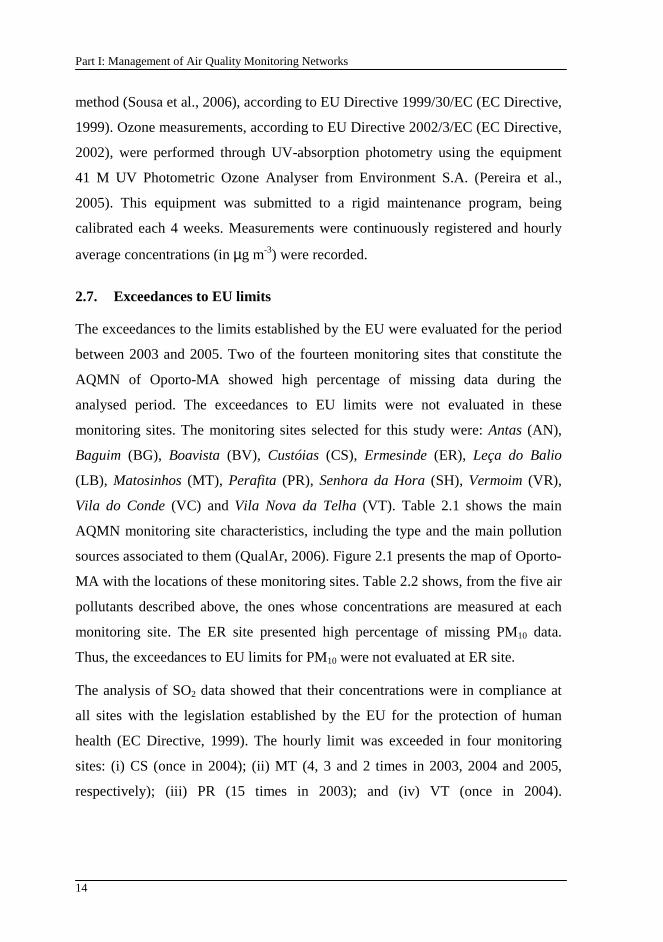
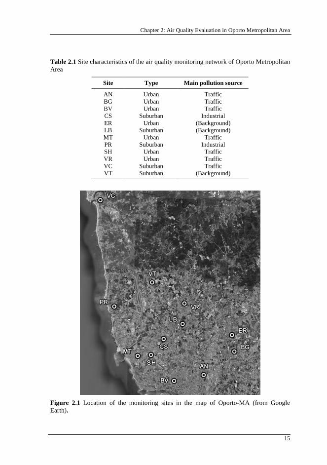
Vila do Conde (VC) and Vila Nova da Telha (VT). Table 2.1 shows the main
AQMN monitoring site characteristics, including the type and the main pollution
sources associated to them (QualAr, 2006). Figure 2.1 presents the map of Oporto-
MA with the locations of these monitoring sites. Table 2.2 shows, from the five air
pollutants described above, the ones whose concentrations are measured at each
monitoring site. The ER site presented high percentage of missing PM10 data.
Thus, the exceedances to EU limits for PM10 were not evaluated at ER site.
The analysis of SO2 data showed that their concentrations were in compliance at
all sites with the legislation established by the EU for the protection of human
health (EC Directive, 1999). The hourly limit was exceeded in four monitoring
sites: (i) CS (once in 2004); (ii) MT (4, 3 and 2 times in 2003, 2004 and 2005,
respectively); (iii) PR (15 times in 2003); and (iv) VT (once in 2004).
Chapter 2: Air Quality Evaluation in Oporto Metropolitan Area
15
Table 2.1 Site characteristics of the air quality monitoring network of Oporto Metropolitan Area
Site Type Main pollution source
AN Urban Traffic BG Urban Traffic BV Urban Traffic CS Suburban Industrial ER Urban (Background) LB Suburban (Background) MT Urban Traffic PR Suburban Industrial SH Urban Traffic VR Urban Traffic VC Suburban Traffic VT Suburban (Background)
Figure 2.1 Location of the monitoring sites in the map of Oporto-MA (from Google Earth).

Part I: Management of Air Quality Monitoring Networks
16
Table 2.2 Air pollutants whose concentrations are measured at each monitoring site
Site SO2 PM10 CO NO2 O3
AN × × × × BG × × × BV × × × × × CS × × × × × ER × × × × LB × × × × × MT × × × × × PR × × × × × SH × × × × VR × × × × × VC × × × × × VT × × × × ×
According to the referred legislation, the SO2 hourly average concentrations limit
of 350 µg m-3 cannot be exceeded more than 24 times a year (~0.3% of the total
number of hours) in order to be in compliance with the norm (EC Directive, 1999).
The PR and MT sites showed the larger number of exceedances during the
analysed period. It is noted that all of the exceedances for the PR site occurred in
2003, which represent ~0.2% of the available hourly average concentrations and
that the correspondent percentages for MT site were even lower (~0.05%). The
daily average concentrations of SO2 were calculated when more than 75% of the
hourly average concentrations were available. The daily limit of SO2
concentrations is 125 µg m-3 and cannot be exceeded more than 3 times a year
(~0.8% of the total number of days) to be in compliance with the norm (EC
Directive, 1999). The daily limit was exceeded only once at the PR site,
representing ~0.3% of the available daily average concentrations. To determine
these exceedances (to hourly and daily limits), the minimum for the percentage of
available data (PAD) was 73%.
Table 2.3 shows the annual averages of SO2 concentrations calculated at each
monitoring site for the years 2003, 2004 and 2005 as well as the correspondent
PAD. It is observed that those annual averages did not change considerably during
the analysed period. MT site showed the highest annual average values
Chapter 2: Air Quality Evaluation in Oporto Metropolitan Area
17
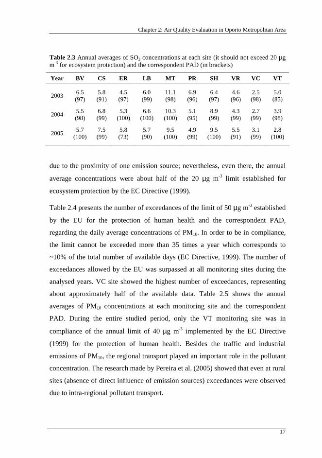
Table 2.3 Annual averages of SO2 concentrations at each site (it should not exceed 20 µg m-3 for ecosystem protection) and the correspondent PAD (in brackets)
Year BV CS ER LB MT PR SH VR VC VT
2003 6.5 (97)
5.8 (91)
4.5 (97)
6.0 (99)
11.1 (98)
6.9 (96)
6.4 (97)
4.6 (96)
2.5 (98)
5.0 (85)
2004 5.5 (98)
6.8 (99)
5.3 (100)
6.6 (100)
10.3 (100)
5.1 (95)
8.9 (99)
4.3 (99)
2.7 (99)
3.9 (98)
2005 5.7
(100) 7.5 (99)
5.8 (73)
5.7 (90)
9.5 (100)
4.9 (99)
9.5 (100)
5.5 (91)
3.1 (99)
2.8 (100)
due to the proximity of one emission source; nevertheless, even there, the annual
average concentrations were about half of the 20 µg m-3 limit established for
ecosystem protection by the EC Directive (1999).
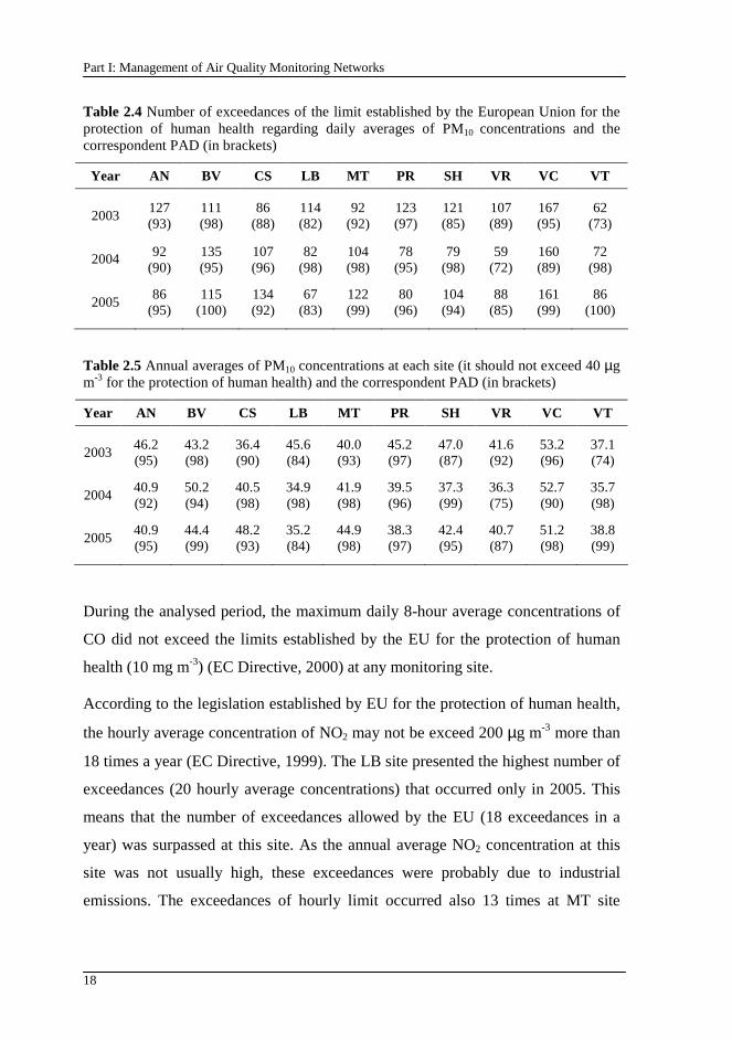
Table 2.4 presents the number of exceedances of the limit of 50 µg m-3 established
by the EU for the protection of human health and the correspondent PAD,
regarding the daily average concentrations of PM10. In order to be in compliance,
the limit cannot be exceeded more than 35 times a year which corresponds to
~10% of the total number of available days (EC Directive, 1999). The number of
exceedances allowed by the EU was surpassed at all monitoring sites during the
analysed years. VC site showed the highest number of exceedances, representing
about approximately half of the available data. Table 2.5 shows the annual
averages of PM10 concentrations at each monitoring site and the correspondent
PAD. During the entire studied period, only the VT monitoring site was in
compliance of the annual limit of 40 µg m-3 implemented by the EC Directive
(1999) for the protection of human health. Besides the traffic and industrial
emissions of PM10, the regional transport played an important role in the pollutant
concentration. The research made by Pereira et al. (2005) showed that even at rural
sites (absence of direct influence of emission sources) exceedances were observed
due to intra-regional pollutant transport.
Part I: Management of Air Quality Monitoring Networks
18
Table 2.4 Number of exceedances of the limit established by the European Union for the protection of human health regarding daily averages of PM10 concentrations and the correspondent PAD (in brackets)
Year AN BV CS LB MT PR SH VR VC VT
2003 127 (93)
111 (98)
86 (88)
114 (82)
92 (92)
123 (97)
121 (85)
107 (89)
167 (95)
62 (73)
2004 92 (90)
135 (95)
107 (96)
82 (98)
104 (98)
78 (95)
79 (98)
59 (72)
160 (89)
72 (98)
2005 86
(95) 115
(100) 134 (92)
67 (83)
122 (99)
80 (96)
104 (94)
88 (85)
161 (99)
86 (100)
Table 2.5 Annual averages of PM10 concentrations at each site (it should not exceed 40 µg m-3 for the protection of human health) and the correspondent PAD (in brackets)
Year AN BV CS LB MT PR SH VR VC VT
2003 46.2 (95)
43.2 (98)
36.4 (90)
45.6 (84)
40.0 (93)
45.2 (97)
47.0 (87)
41.6 (92)
53.2 (96)
37.1 (74)
2004 40.9 (92)
50.2 (94)
40.5 (98)
34.9 (98)
41.9 (98)
39.5 (96)
37.3 (99)
36.3 (75)
52.7 (90)
35.7 (98)
2005 40.9 (95)
44.4 (99)
48.2 (93)
35.2 (84)
44.9 (98)
38.3 (97)
42.4 (95)
40.7 (87)
51.2 (98)
38.8 (99)
During the analysed period, the maximum daily 8-hour average concentrations of
CO did not exceed the limits established by the EU for the protection of human
health (10 mg m-3) (EC Directive, 2000) at any monitoring site.
According to the legislation established by EU for the protection of human health,
the hourly average concentration of NO2 may not be exceed 200 µg m-3 more than
18 times a year (EC Directive, 1999). The LB site presented the highest number of
exceedances (20 hourly average concentrations) that occurred only in 2005. This
means that the number of exceedances allowed by the EU (18 exceedances in a
year) was surpassed at this site. As the annual average NO2 concentration at this
site was not usually high, these exceedances were probably due to industrial
emissions. The exceedances of hourly limit occurred also 13 times at MT site
Chapter 2: Air Quality Evaluation in Oporto Metropolitan Area
19
(2005), 6 times at VR site (2004), 4 times at AN and BV sites (2005) and twice at
BG site (2005). To determine these exceedances, the minimum for the percentage
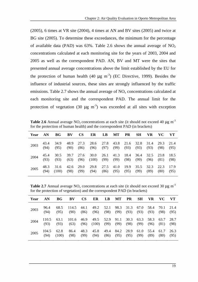
of available data (PAD) was 63%. Table 2.6 shows the annual average of NO2
concentrations calculated at each monitoring site for the years of 2003, 2004 and
2005 as well as the correspondent PAD. AN, BV and MT were the sites that
presented annual average concentrations above the limit established by the EU for
the protection of human health (40 µg m-3) (EC Directive, 1999). Besides the
influence of industrial sources, these sites are strongly influenced by the traffic
emissions. Table 2.7 shows the annual average of NOx concentrations calculated at
each monitoring site and the correspondent PAD. The annual limit for the
protection of vegetation (30 µg m-3) was exceeded at all sites with exception
Table 2.6 Annual average NO2 concentrations at each site (it should not exceed 40 µg m-3 for the protection of human health) and the correspondent PAD (in brackets)
Year AN BG BV CS ER LB MT PR SH VR VC VT
2003 43.4 (94)
34.9 (95)
48.9 (90)
27.3 (86)
28.6 (96)
27.8 (97)
43.8 (99)
21.6 (93)
32.8 (93)
31.4 (93)
29.3 (98)
21.4 (95)
2004 45.4 (93)
30.5 (93)
39.7 (63)
27.6 (96)
30.0 (100)
26.1 (99)
41.3 (99)
18.4 (98)
36.4 (99)
32.5 (96)
23.8 (81)
18.5 (98)
2005 48.3 (94)
31.6 (100)
42.6 (98)
29.0 (99)
29.8 (94)
27.5 (86)
41.0 (95)
19.9 (95)
35.5 (99)
32.3 (89)
22.3 (80)
17.9 (95)
Table 2.7 Annual average NOx concentrations at each site (it should not exceed 30 µg m-3 for the protection of vegetation) and the correspondent PAD (in brackets)
Year AN BG BV CS ER LB MT PR SH VR VC VT
2003 96.4 (94)
68.5 (95)
114.5 (90)
44.1 (86)
49.2 (96)
52.1 (98)
98.3 (99)
31.3 (93)
67.0 (93)
58.4 (93)
70.1 (98)
21.4 (95)
2004 110.5 (93)
63.1 (93)
101.6 (63)
46.9 (96)
49.5 (100)
52.9 (99)
91.1 (99)
30.3 (98)
63.3 (99)
58.3 (96)
63.7 (81)
28.7 (98)
2005 104.5 (94)
62.8 (100)
86.4 (98)
48.3 (99)
45.8 (94)
49.4 (86)
84.2 (95)
28.9 (95)
61.0 (99)
55.4 (89)
61.7 (80)
26.3 (95)
Part I: Management of Air Quality Monitoring Networks
20
of VT site (during the entire period) and PR site (in 2005) (EC Directive, 1999).
As it happened with NO2, AN, BV and MT sites presented the highest annual
average concentrations of NOx. For both pollutants, there was not a significant
variation of their annual average concentration during the analysed period.
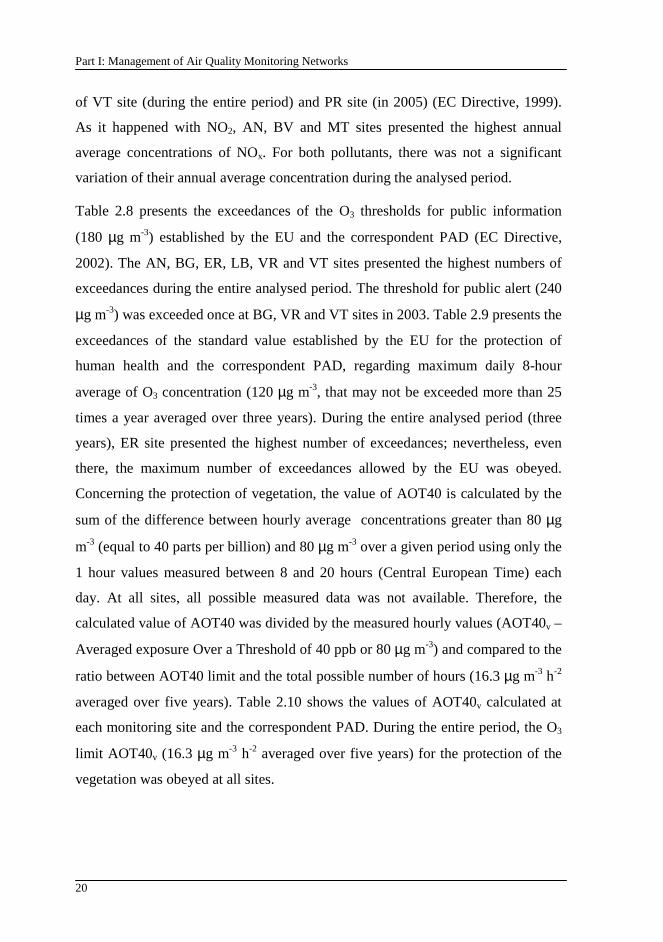
Table 2.8 presents the exceedances of the O3 thresholds for public information
(180 µg m-3) established by the EU and the correspondent PAD (EC Directive,
2002). The AN, BG, ER, LB, VR and VT sites presented the highest numbers of
exceedances during the entire analysed period. The threshold for public alert (240
µg m-3) was exceeded once at BG, VR and VT sites in 2003. Table 2.9 presents the
exceedances of the standard value established by the EU for the protection of
human health and the correspondent PAD, regarding maximum daily 8-hour
average of O3 concentration (120 µg m-3, that may not be exceeded more than 25
times a year averaged over three years). During the entire analysed period (three
years), ER site presented the highest number of exceedances; nevertheless, even
there, the maximum number of exceedances allowed by the EU was obeyed.
Concerning the protection of vegetation, the value of AOT40 is calculated by the
sum of the difference between hourly average concentrations greater than 80 µg
m-3 (equal to 40 parts per billion) and 80 µg m-3 over a given period using only the
1 hour values measured between 8 and 20 hours (Central European Time) each
day. At all sites, all possible measured data was not available. Therefore, the
calculated value of AOT40 was divided by the measured hourly values (AOT40v –
Averaged exposure Over a Threshold of 40 ppb or 80 µg m-3) and compared to the
ratio between AOT40 limit and the total possible number of hours (16.3 µg m-3 h-2
averaged over five years). Table 2.10 shows the values of AOT40v calculated at
each monitoring site and the correspondent PAD. During the entire period, the O3
limit AOT40v (16.3 µg m-3 h-2 averaged over five years) for the protection of the
vegetation was obeyed at all sites.
Chapter 2: Air Quality Evaluation in Oporto Metropolitan Area
21
Table 2.8 Exceedances of the O3 thresholds for public information (180 µg m-3) established by the European Union and the correspondent PAD (in brackets)
Year AN BG BV CS ER LB MT PR VR VC VT
2003 6
(86) 5
(93) 2
(95) 0
(92) 4
(97) 0
(47) 0
(100) 0
(99) 5
(96) 0
(98) 7
(95)
2004 2
(97) 1
(100) 0
(99) 3
(100) 4
(99) 1
(94) 0
(100) 5
(98) 3
(99) 1
(99) 4
(98)
2005 10
(99) 7
(100) 0
(100) 2
(53) 17
(100) 27
(69) 0
(90) 1
(100) 8
(91) 0
(98) 12
(100)
Table 2.9 Exceedances of the standard value established by the European Union for human health protection, regarding maximum daily 8-hour average of O3 concentration and the correspondent PAD (in brackets)
Year AN BG BV CS ER LB MT PR VR VC VT
2003 7
(87) 9
(94) 1
(96) 5
(94) 11
(98) 0
(47) 1
(100) 3
(100) 10
(98) 5
(98) 12
(97)
2004 4
(98) 3
(100) 1
(99) 7
(100) 11
(100) 3
(95) 2
(100) 11
(100) 9
(100) 2
(100) 6
(99)
2005 7
(100) 9
(100) 3
(100) 1
(53) 23
(100) 19
(70) 6
(91) 13
(100) 17
(92) 9
(99) 17
(100)
Table 2.10 Values of AOT40v at each site (it should not exceed 16.3 µg m-3 h-2 averaged over five years, for the protection of vegetation) and the correspondent PAD (in brackets)
Year AN BG BV CS ER LB MT PR VR VC VT
2003 3.5 (95)
4.0 (99)
1.8 (100)
5.2 (96)
7.7 (98)
- 1.7 (99)
4.5 (99)
6.2 (88)
4.7 (100)
7.6 (95)
2004 3.4 (90)
5.4 (100)
1.4 (96)
7.9 (99)
8.0 (99)
3.5 (82)
2.5 (99)
9.2 (99)
4.6 (100)
4.3 (99)
5.8 (98)
2005 3.4
(100) 5.9 (99)
1.4 (99)
5.0 (75)
8.5 (100)
14.5 (75)
2.8 (69)
6.2 (98)
11.9 (99)
5.2 (99)
8.2 (100)
2.8. Conclusions
The analysis to the exceedances to EU limits showed that Oporto-MA presents
lower levels of CO and SO2 concentrations. As it is a region strongly influenced
by traffic, the concentrations of NOx and PM10 surpassed the limits at almost all

Part I: Management of Air Quality Monitoring Networks
22
monitoring sites. For NO2, the concerning monitoring sites were AN, BV, LB and
MT. With higher levels of NOx, the equilibrium chemical reaction evolving NOx
and O3 limits the concentrations of the last one. Despite this fact, the limits relative
to O3 concentrations regarding the protection of human health were surpassed at
all sites.
23
Chapter 3
3. Characterization of Air Pollution Behaviours
The air quality monitoring of air pollutant levels should be adequately managed in any air quality monitoring network. The number of monitoring sites that constitute the network should be optimized helping to reduce expenses; but at the same time guarantying the adequate characterization of the regional air quality. This means that only one monitoring site should operate in an area characterized by specific air pollution behaviour. This chapter shows how principal component and cluster analyses can be applied to define the minimum number of monitoring sites that should operate in an air quality monitoring network. Additionally, the location of main emission sources was identified based on the wind direction.
The contents of this chapter were adapted from: (i) Pires, J.C.M., Sousa, S.I.V., Pereira, M.C., Alvim-Ferraz, M.C.M., Martins, F.G., 2008. Management of Air Quality Monitoring using Principal Component and Cluster Analysis – Part I: SO2 and PM10. Atmospheric Environment 42 (6), 1249-1260; and (ii) Pires, J.C.M., Sousa, S.I.V., Pereira, M.C., Alvim-Ferraz, M.C.M., Martins, F.G., 2008. Management of Air Quality Monitoring using Principal Component and Cluster Analysis – Part II: CO, NO2 and O3. Atmospheric Environment 42 (6), 1261-1274.
3.1. Introduction
Principal component analysis (PCA) is a statistical technique that creates new
variables, called principal components (PCs) that are orthogonal and uncorrelated
to each other. These PCs are linear combinations of the original variables and are
obtained in such a way that the first PC explains the largest fraction of the original
data variability; the second PC explains a lesser fraction of the data variance than
the first PC and so forth (Abdul-Wahab et al., 2005; Sousa et al., 2007; Wang and
Xiao, 2004). To better clarify the influence of each original variable in the PCs, a
Part I: Management of Air Quality Monitoring Networks
24
rotational algorithm such as varimax rotation is generally applied to obtain the
rotated factor loadings that represent the contribution of each variable to a specific
PC. PCA procedure is described in more detail in Chapter 6. Although PCA is
mostly used for reducing the multiple dimensions associated to multivariate
analyses, it was applied in this study as a method of classification, in order to
group the monitoring sites into classes (PCs) having the similar air pollution
behaviour.
Cluster analysis (CA) is a classification method used to divide the data in classes
or clusters. Its main aim is to establish a set of clusters such that objects in the
same cluster (CL) are similar to each other and different from objects located in
another clusters (Manly, 1994). The ideal number of clusters may be determined
graphically through a dendrogram, a tree diagram commonly used in CA (Manly,
1994; McKenna, 2003). This classification method can also be useful for data
reduction.
PCA and CA have been used in many studies aiming the management of water
monitoring networks (Kannel et al., 2007; Mendiguchía et al., 2004; Shrestha and
Kazama, 2007; Singh et al., 2004; Singh et al., 2005). Nevertheless, as far as it is
known by the author, only the research made by Gramsch et al. (2006) has applied
CA for the analysis of air quality management. Their study determined the
seasonal trends and spatial distribution of PM10 and O3 for Santiago de Chile,
concluding that the city had four large sectors with dissimilar air pollution
behaviours.
The global aim of this chapter was to evaluate the performance of PCA and CA for
the management of air pollutant concentrations monitoring with the following
specific objectives: (i) to identify city areas with similar air pollution behaviour;
and (ii) to locate main emission sources.
Chapter 3: Characterization of Air Pollution Behaviours
25
3.2. Air quality data
PCA and CA were applied to the analysis of the air pollutant (SO2, PM10, CO, NO2
and O3) concentrations collected in the AQMN of Oporto-MA, from January 2003
to December 2005. To be able to apply these statistical methods, hourly
concentrations need to be available at all sites in the same time period. For SO2,
the number of available hourly data at each monitoring site were 5281, 7761 and
5355 for the 2003, 2004 and 2005 years, respectively; for PM10, the number of
available hourly data at each monitoring site were 4490, 4369 and 5548; for CO,
the number of available hourly data at each monitoring site were 2681, 3478 and
2565; for NO2, the number of available hourly data at each monitoring site were
4277, 3482 and 4675; and for O3, the number of available hourly data at each site
were 1967, 7390 and 1943. Concentration values were Z standardized to have zero
mean and unit standard deviation.
3.3. Results and discussion
PCA was applied as a non-parametric method of classification in order to group
the monitoring sites into classes having similar air pollution behaviours and
differing from those in other classes. Table 3.1 shows the main results of the PCA
application for both pollutants at all sites. Considering eigenvalues greater than 1
(Kaiser criterion; Yidana et al., 2008), only the first four PCs that explain 63.8%
of the original data variance need to be taken into account for analyzing the SO2
concentrations. However, in order to consider a cumulative variance greater than
75%, the PC5 and PC6 components were selected (having eigenvalues of 0.91 and
0.81, respectively), in which case 81.0% of the data variance was explained.
Considering the same criterion, two PCs could be selected for CO concentrations,
explaining 71.6% of variance of the original data. One more PC with eigeinvalue
close to 1 (0.71) could be selected to achieve at least 75% of the original data
variance, resulting in 78.1% of the total variance. On the other hand, for PM10,
NO2 and O3 concentrations, two PCs were selected for each pollutant and
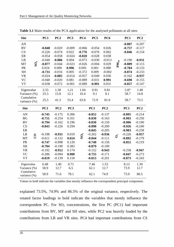
Part I: Management of Air Quality Monitoring Networks
26
Table 3.1 Main results of the PCA application for the analysed pollutants at all sites
Site PC1 PC2 PC3 PC4 PC5 PC6 PC1 PC2
AN -0.807 -0.207 BV -0.848 -0.020 -0.009 -0.066 -0.054 0.026 -0.757 -0.117 CS -0.226 -0.074 0.022 -0.776 -0.076 0.062 -0.846 -0.154 ER -0.054 -0.058 -0.024 -0.820 -0.028 0.038 LB -0.040 -0.886 0.004 -0.073 -0.030 -0.013 -0.190 -0.931 MT -0.877 -0.044 -0.023 -0.026 -0.004 0.029 -0.889 -0.115 PR 0.024 0.009 0.996 0.005 0.001 0.080 -0.784 -0.133 SH -0.731 -0.016 0.005 -0.372 0.009 -0.002 -0.874 -0.233 VR -0.024 -0.885 -0.014 -0.057 -0.049 0.036 -0.162 -0.937 VC -0.040 -0.020 0.081 -0.089 -0.031 0.991 -0.698 -0.155 VT
SO
2
-0.038 -0.072 -0.001 -0.089 -0.991 0.031
PM
10
-0.857 -0.147
Eigenvalue 2.55 1.58 1.21 1.04 0.91 0.81 5.87 1.48 Variance (%) 25.5 15.8 12.1 10.4 9.1 8.1 58.7 14.8 Cumulative variance (%) 25.5 41.3 53.4 63.8 72.9 81.0 58.7 73.5
Site PC1 PC2 PC3 PC1 PC2 PC1 PC2
AN -0.745 -0.175 0.306 -0.852 -0.137 -0.895 -0.214 BG -0.751 -0.254 0.351 -0.830 -0.163 -0.903 -0.250 BV -0.794 -0.162 0.196 -0.830 -0.150 -0.906 -0.190 CS -0.843 -0.226 0.294 -0.898 -0.200 -0.926 -0.240 ER -0.845 -0.205 -0.903 -0.258 LB -0.198 -0.931 0.019 -0.202 -0.936 -0.226 -0.957 MT -0.611 -0.132 0.654 -0.844 -0.111 -0.892 -0.179 PR -0.747 -0.098 0.120 -0.740 -0.156 -0.851 -0.219 SH -0.784 -0.190 0.383 -0.879 -0.100 VR -0.192 -0.912 0.174 -0.152 -0.943 -0.258 -0.947 VC -0.286 -0.094 0.900 -0.755 -0.171 -0.847 -0.273 VT
CO
-0.819 -0.139 0.159
NO
2
-0.813 -0.201
O3
-0.873 -0.243
Eigenvalue 6.48 1.40 0.71 7.46 1.53 8.13 1.39 Variance (%) 58.9 12.7 6.5 62.1 12.7 73.9 12.7 Cumulative variance (%) 58.9 71.6 78.1 62.1 74.9 73.9 86.5
Values in bold indicate the variables that mostly influence the correspondent principal component.
explained 73.5%, 74.9% and 86.5% of the original variance, respectively. The
rotated factor loadings in bold indicate the variables that mostly influence the
correspondent PC. For SO2 concentrations, the first PC (PC1) had important
contributions from BV, MT and SH sites, while PC2 was heavily loaded by the
contributions from LB and VR sites. PC4 had important contributions from CS
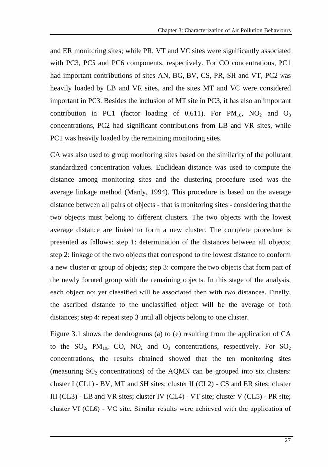
Chapter 3: Characterization of Air Pollution Behaviours
27
and ER monitoring sites; while PR, VT and VC sites were significantly associated
with PC3, PC5 and PC6 components, respectively. For CO concentrations, PC1
had important contributions of sites AN, BG, BV, CS, PR, SH and VT, PC2 was
heavily loaded by LB and VR sites, and the sites MT and VC were considered
important in PC3. Besides the inclusion of MT site in PC3, it has also an important
contribution in PC1 (factor loading of 0.611). For PM10, NO2 and O3
concentrations, PC2 had significant contributions from LB and VR sites, while
PC1 was heavily loaded by the remaining monitoring sites.
CA was also used to group monitoring sites based on the similarity of the pollutant
standardized concentration values. Euclidean distance was used to compute the
distance among monitoring sites and the clustering procedure used was the
average linkage method (Manly, 1994). This procedure is based on the average
distance between all pairs of objects - that is monitoring sites - considering that the
two objects must belong to different clusters. The two objects with the lowest
average distance are linked to form a new cluster. The complete procedure is
presented as follows: step 1: determination of the distances between all objects;
step 2: linkage of the two objects that correspond to the lowest distance to conform
a new cluster or group of objects; step 3: compare the two objects that form part of
the newly formed group with the remaining objects. In this stage of the analysis,
each object not yet classified will be associated then with two distances. Finally,
the ascribed distance to the unclassified object will be the average of both
distances; step 4: repeat step 3 until all objects belong to one cluster.
Figure 3.1 shows the dendrograms (a) to (e) resulting from the application of CA
to the SO2, PM10, CO, NO2 and O3 concentrations, respectively. For SO2
concentrations, the results obtained showed that the ten monitoring sites
(measuring SO2 concentrations) of the AQMN can be grouped into six clusters:
cluster I (CL1) - BV, MT and SH sites; cluster II (CL2) - CS and ER sites; cluster
III (CL3) - LB and VR sites; cluster IV (CL4) - VT site; cluster V (CL5) - PR site;
cluster VI (CL6) - VC site. Similar results were achieved with the application of
Part I: Management of Air Quality Monitoring Networks
28
a b
c d
e
Figure 3.1 Dendrograms resulting from the application of CA to the (a) SO2, (b) PM10, (c) CO, (d) NO2 and (e) O3 concentrations.
PCA, where the PC1, PC2, PC3, PC4, PC5 and PC6 principal components
corresponded exactly to the CL1, CL3, CL5, CL2, CL4 and CL6 clusters of the
Chapter 3: Characterization of Air Pollution Behaviours
29
CA, respectively. For the PM10 concentrations, similar results were achieved with
PCA, with the PC1 and PC2 principal components of the PCA corresponding
exactly to the CL2 and CL1 clusters of the CA, respectively. For CO
concentrations, the results obtained showed that the eleven monitoring sites of the
AQMN could be coupled into three clusters: cluster I (CL1) – AN, BG, BV, CS,
PR, SH and VT sites; cluster II (CL2) – MT and VC sites; cluster III (CL3) – LB
and VR sites. Similar results were achieved with PCA, where PC1, PC2 and PC3
corresponded to CL1, CL3 and CL2, respectively. For NO2 concentrations, the
twelve sites could be also coupled into three clusters: cluster I (CL1) – sites BG,
CS, ER, PR, SH, VC and VT; cluster II (CL2) –sites LB and VR; cluster III (CL3)
–sites AN, BV and MT. For this pollutant, PCA and CA did not achieve the same
results. PC2 corresponded to CL2, but the sites coupled in PC1 were divided into
CL1 and CL3. Furthermore, for O3 concentrations, PCA and CA also achieved
similar results, with PC1 and PC2 corresponding to CL1 and CL2, respectively.
Therefore, it was possible to conclude that the O3 concentrations monitored at the
eleven sites could be coupled in no more than two groups.
Figure 3.2 (from a to f) shows the average daily profile of the hourly average SO2
concentrations at the monitoring sites grouped by the correspondent PC/CL
category. Similar behaviours of SO2 pollution can be observed in sites belonging
to the same PC/CL category. Figure 3.3 (from a to b) shows the daily profile of the
hourly average PM10 concentrations grouped by the correspondent PC/CL
category. For the second group (PC2/CL1 category), the monitoring sites had
similar pollution profile. Nevertheless, and for the first group (PC1/CL2), the sites
had the same profile until 17 hours, but between 17 and 22 hours VC site showed a
peak of PM10 concentration. The inclusion of VC site in this group by the PCA is
related to the low proportion of the original data variance explained by the first
two PCs (communality of 0.51). In CA, this is explained by the correspondent
Euclidean distance of the VC site, which was greater than in other sites belonging
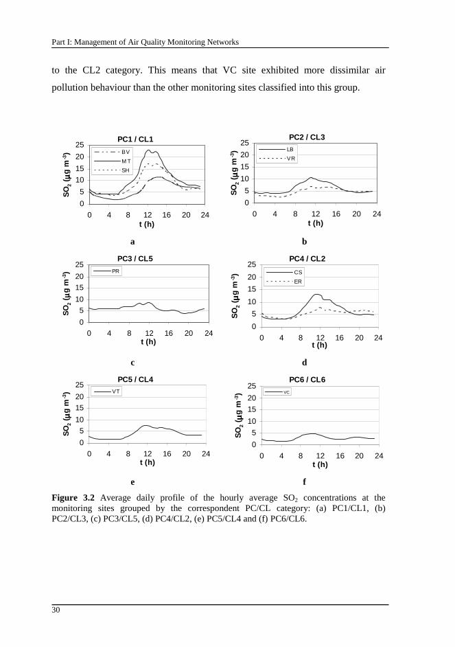
Part I: Management of Air Quality Monitoring Networks
30
to the CL2 category. This means that VC site exhibited more dissimilar air
pollution behaviour than the other monitoring sites classified into this group.
PC1 / CL1
0
5
10
15
20
25
0 4 8 12 16 20 24t (h)
SO
2 ( µµ µµ
g m
-3) BV
M T
SH
PC2 / CL3
0
5
10
15
20
25
0 4 8 12 16 20 24t (h)
SO
2 ( µµ µµ
g m
-3) LB
VR
a b
PC3 / CL5
0
5
10
15
20
25
0 4 8 12 16 20 24t (h)
SO
2 ( µµ µµ
g m
-3) PR
PC4 / CL2
0
5
10
15
20
25
0 4 8 12 16 20 24t (h)
SO
2 ( µµ µµ
g m
-3) CS
ER
c d
PC5 / CL4
0
5
10
15
20
25
0 4 8 12 16 20 24t (h)
SO
2 ( µµ µµ
g m
-3) VT
PC6 / CL6
0
5
10
15
20
25
0 4 8 12 16 20 24t (h)
SO
2 ( µµ µµ
g m
-3) VC
e f
Figure 3.2 Average daily profile of the hourly average SO2 concentrations at the monitoring sites grouped by the correspondent PC/CL category: (a) PC1/CL1, (b) PC2/CL3, (c) PC3/CL5, (d) PC4/CL2, (e) PC5/CL4 and (f) PC6/CL6.
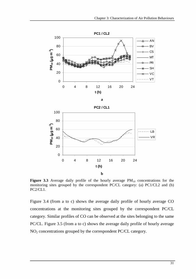
Chapter 3: Characterization of Air Pollution Behaviours
31
PC1 / CL2
0
20
40
60
80
100
0 4 8 12 16 20 24
t (h)
PM
10 ( µµ µµ
g m
-3)
AN
BV
CS
MT
PR
SH
VC
VT
a
PC2 / CL1
0
20
40
60
80
100
0 4 8 12 16 20 24
t (h)
PM
10 ( µµ µµ
g m
-3)
LB
VR
b
Figure 3.3 Average daily profile of the hourly average PM10 concentrations for the monitoring sites grouped by the correspondent PC/CL category: (a) PC1/CL2 and (b) PC2/CL1.
Figure 3.4 (from a to c) shows the average daily profile of hourly average CO
concentrations at the monitoring sites grouped by the correspondent PC/CL
category. Similar profiles of CO can be observed at the sites belonging to the same
PC/CL. Figure 3.5 (from a to c) shows the average daily profile of hourly average
NO2 concentrations grouped by the correspondent PC/CL category.
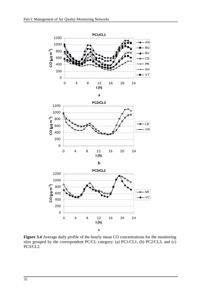
Part I: Management of Air Quality Monitoring Networks
32
PC1/CL1
0
200
400
600
800
1000
1200
0 4 8 12 16 20 24t (h)
CO
( µµ µµg
m-3
)
AN
BG
BV
CS
PR
SH
VT
a
PC2/CL3
0
200
400
600
800
1000
1200
0 4 8 12 16 20 24t (h)
CO
( µµ µµg
m-3
)
LB
VR
b
PC3/CL2
0
200
400
600
800
1000
1200
0 4 8 12 16 20 24t (h)
CO
( µµ µµg
m-3
)
MT
VC
c
Figure 3.4 Average daily profile of the hourly mean CO concentrations for the monitoring sites grouped by the correspondent PC/CL category: (a) PC1/CL1, (b) PC2/CL3, and (c) PC3/CL2.
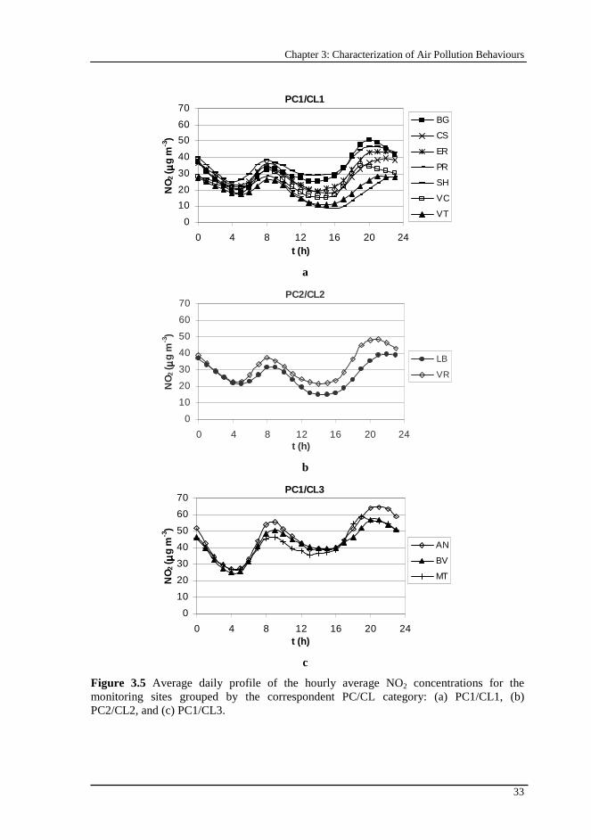
Chapter 3: Characterization of Air Pollution Behaviours
33
PC1/CL1
0
10
20
30
40
50
60
70
0 4 8 12 16 20 24t (h)
NO
2 (µµ µµ
g m
-3)
BG
CS
ER
PR
SH
VC
VT
a
PC2/CL2
0
10
20
30
40
50
60
70
0 4 8 12 16 20 24t (h)
NO
2 (µµ µµ
g m
-3)
LB
VR
b
PC1/CL3
0
10
20
30
40
50
60
70
0 4 8 12 16 20 24t (h)
NO
2 (µµ µµ
g m
-3)
AN
BV
MT
c
Figure 3.5 Average daily profile of the hourly average NO2 concentrations for the monitoring sites grouped by the correspondent PC/CL category: (a) PC1/CL1, (b) PC2/CL2, and (c) PC1/CL3.
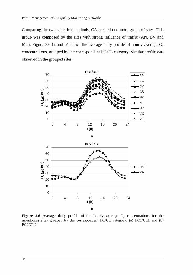
Part I: Management of Air Quality Monitoring Networks
34
Comparing the two statistical methods, CA created one more group of sites. This
group was composed by the sites with strong influence of traffic (AN, BV and
MT). Figure 3.6 (a and b) shows the average daily profile of hourly average O3
concentrations, grouped by the correspondent PC/CL category. Similar profile was
observed in the grouped sites.
PC1/CL1
0
10
20
30
40
50
60
70
0 4 8 12 16 20 24t (h)
O3 (
µµ µµg
m-3
)
AN
BG
BV
CS
ER
MT
PR
VC
VT
a
PC2/CL2
0
10
20
30
40
50
60
70
0 4 8 12 16 20 24t (h)
O3 (
µµ µµg
m-3
)
LB
VR
b
Figure 3.6 Average daily profile of the hourly average O3 concentrations for the monitoring sites grouped by the correspondent PC/CL category: (a) PC1/CL1 and (b) PC2/CL2.
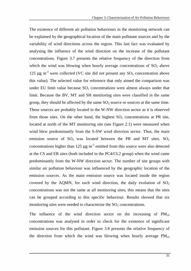
Chapter 3: Characterization of Air Pollution Behaviours
35
The existence of different air pollution behaviours in the monitoring network can
be explained by the geographical location of the main pollutant sources and by the
variability of wind directions across the region. This last fact was evaluated by
analysing the influence of the wind direction on the increase of the pollutant
concentrations. Figure 3.7 presents the relative frequency of the direction from
which the wind was blowing when hourly average concentrations of SO2 above
125 µg m-3 were collected (VC site did not present any SO2 concentration above
this value). The selected value for reference that only aimed the comparison was
under EU limit value because SO2 concentrations were almost always under that
limit. Because the BV, MT and SH monitoring sites were classified in the same
group, they should be affected by the same SO2 source or sources at the same time.
These sources are probably located in the W-NW direction sector as it is observed
from those sites. On the other hand, the highest SO2 concentrations at PR site,
located at north of the MT monitoring site (see Figure 2.1) were measured when
wind blew predominantly from the S-SW wind direction sector. Thus, the main
emission source of SO2 was located between the PR and MT sites. SO2
concentrations higher than 125 µg m-3 emitted from this source were also detected
at the CS and ER sites (both included in the PC4/CL2 group) when the wind came
predominantly from the W-NW direction sector. The number of site groups with
similar air pollution behaviour was influenced by the geographic location of the
emission sources. As the main emission source was located inside the region
covered by the AQMN, for each wind direction, the daily evolution of SO2
concentrations was not the same at all monitoring sites; this means that the sites
can be grouped according to this specific behaviour. Results showed that six
monitoring sites were needed to characterize the SO2 concentrations.
The influence of the wind direction sector on the increasing of PM10
concentrations was analysed in order to check for the existence of significant
emission sources for this pollutant. Figure 3.8 presents the relative frequency of
the direction from which the wind was blowing when hourly average PM10
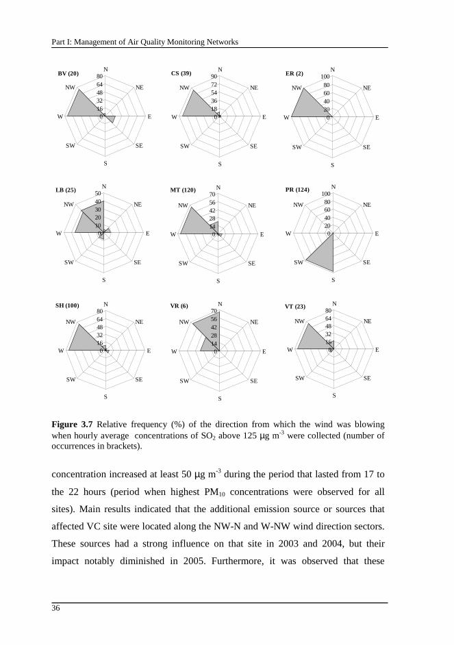
Part I: Management of Air Quality Monitoring Networks
36
BV (20)
01632486480
N
NE
E
SE
S
SW
W
NW
CS (39)
01836547290
N
NE
E
SE
S
SW
W
NW
ER (2)
020406080
100N
NE
E
SE
S
SW
W
NW
LB (25)
01020304050
N
NE
E
SE
S
SW
W
NW
MT (120)
01428425670
N
NE
E
SE
S
SW
W
NW
PR (124)
020406080
100N
NE
E
SE
S
SW
W
NW
SH (100)
01632486480
N
NE
E
SE
S
SW
W
NW
VR (6)
01428425670
N
NE
E
SE
S
SW
W
NW
VT (23)
01632486480
N
NE
E
SE
S
SW
W
NW
Figure 3.7 Relative frequency (%) of the direction from which the wind was blowing when hourly average concentrations of SO2 above 125 µg m-3 were collected (number of occurrences in brackets).
concentration increased at least 50 µg m-3 during the period that lasted from 17 to
the 22 hours (period when highest PM10 concentrations were observed for all
sites). Main results indicated that the additional emission source or sources that
affected VC site were located along the NW-N and W-NW wind direction sectors.
These sources had a strong influence on that site in 2003 and 2004, but their
impact notably diminished in 2005. Furthermore, it was observed that these
Chapter 3: Characterization of Air Pollution Behaviours
37
AN (48)
01224364860
N
NE
E
SE
S
SW
W
NW
BV (83)
01020304050
N
NE
E
SE
S
SW
W
NW
CS (114)
01224364860
N
NE
E
SE
S
SW
W
NW
LB (86)
01020304050
N
NE
E
SE
S
SW
W
NW
MT (73)
01224364860
N
NE
E
SE
S
SW
W
NW
PR (95)
01020304050
N
NE
E
SE
S
SW
W
NW
SH (77)
01224364860
N
NE
E
SE
S
SW
W
NW
VR (94)
01020304050
N
NE
E
SE
S
SW
W
NW
VC (198)
01020304050
N
NE
E
SE
S
SW
W
NW
VT (55)
01020304050
N
NE
E
SE
S
SW
W
NW
Figure 3.8 Relative frequency (%) of the direction from which the wind was blowing when hourly average concentrations of PM10 increased at least 50 µg m-3 during the period that lasted from 17 to the 22 hours (number of occurrences in brackets).
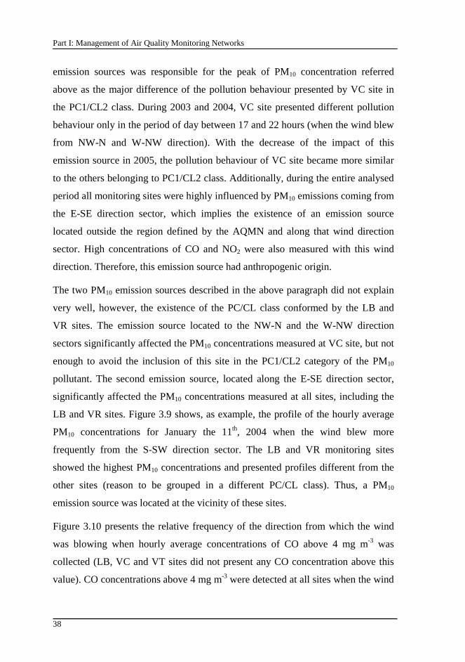
Part I: Management of Air Quality Monitoring Networks
38
emission sources was responsible for the peak of PM10 concentration referred
above as the major difference of the pollution behaviour presented by VC site in
the PC1/CL2 class. During 2003 and 2004, VC site presented different pollution
behaviour only in the period of day between 17 and 22 hours (when the wind blew
from NW-N and W-NW direction). With the decrease of the impact of this
emission source in 2005, the pollution behaviour of VC site became more similar
to the others belonging to PC1/CL2 class. Additionally, during the entire analysed
period all monitoring sites were highly influenced by PM10 emissions coming from
the E-SE direction sector, which implies the existence of an emission source
located outside the region defined by the AQMN and along that wind direction
sector. High concentrations of CO and NO2 were also measured with this wind
direction. Therefore, this emission source had anthropogenic origin.
The two PM10 emission sources described in the above paragraph did not explain
very well, however, the existence of the PC/CL class conformed by the LB and
VR sites. The emission source located to the NW-N and the W-NW direction
sectors significantly affected the PM10 concentrations measured at VC site, but not
enough to avoid the inclusion of this site in the PC1/CL2 category of the PM10
pollutant. The second emission source, located along the E-SE direction sector,
significantly affected the PM10 concentrations measured at all sites, including the
LB and VR sites. Figure 3.9 shows, as example, the profile of the hourly average
PM10 concentrations for January the 11th, 2004 when the wind blew more
frequently from the S-SW direction sector. The LB and VR monitoring sites
showed the highest PM10 concentrations and presented profiles different from the
other sites (reason to be grouped in a different PC/CL class). Thus, a PM10
emission source was located at the vicinity of these sites.
Figure 3.10 presents the relative frequency of the direction from which the wind
was blowing when hourly average concentrations of CO above 4 mg m-3 was
collected (LB, VC and VT sites did not present any CO concentration above this
value). CO concentrations above 4 mg m-3 were detected at all sites when the wind
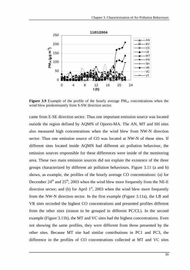
Chapter 3: Characterization of Air Pollution Behaviours
39
11/01/2004
0
50
100
150
200
250
0 4 8 12 16 20 24t (h)
PM
10 ( µµ µµ
g m
-3)
ANBVCSLBMTPRSHVRVCVT
Figure 3.9 Example of the profile of the hourly average PM10 concentrations when the wind blew predominantly from S-SW direction sector.
came from E-SE direction sector. Thus one important emission source was located
outside the region defined by AQMN of Oporto-MA. The AN, MT and SH sites
also measured high concentrations when the wind blew from NW-N direction
sector. Thus one emission source of CO was located at NW-N of these sites. If
different sites located inside AQMN had different air pollution behaviour, the
emission sources responsible for these differences were inside of the monitoring
area. These two main emission sources did not explain the existence of the three
groups characterized by different air pollution behaviours. Figure 3.11 (a and b)
shows, as example, the profiles of the hourly average CO concentrations: (a) for
December 24th and 25th, 2003 when the wind blew more frequently from the NE-E
direction sector; and (b) for April 1st, 2003 when the wind blew more frequently
from the NW-N direction sector. In the first example (Figure 3.11a), the LB and
VR sites recorded the highest CO concentrations and presented profiles different
from the other sites (reason to be grouped in different PC/CL). In the second
example (Figure 3.11b), the MT and VC sites had the highest concentrations. Even
not showing the same profiles, they were different from those presented by the
other sites. Because MT site had similar contributions in PC1 and PC3, the
difference in the profiles of CO concentrations collected at MT and VC sites
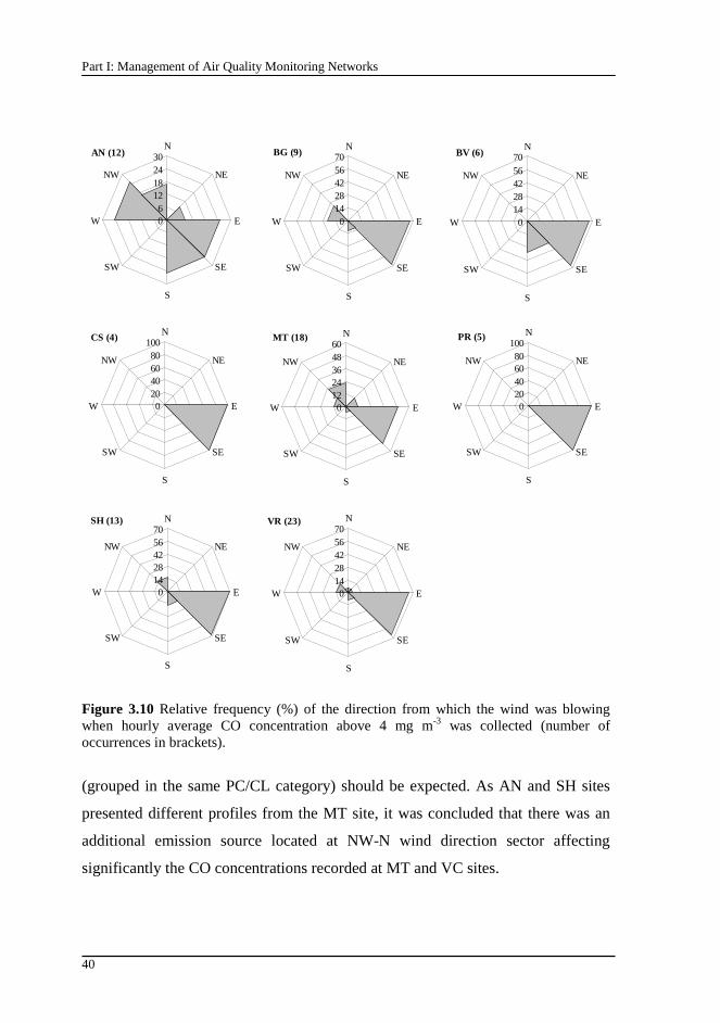
Part I: Management of Air Quality Monitoring Networks
40
AN (12)
06
12182430
N
NE
E
SE
S
SW
W
NW
BG (9)
01428425670
N
NE
E
SE
S
SW
W
NW
BV (6)
01428425670
N
NE
E
SE
S
SW
W
NW
CS (4)
020406080
100N
NE
E
SE
S
SW
W
NW
MT (18)
01224364860
N
NE
E
SE
S
SW
W
NW
PR (5)
020406080
100N
NE
E
SE
S
SW
W
NW
SH (13)
01428425670
N
NE
E
SE
S
SW
W
NW
VR (23)
01428425670
N
NE
E
SE
S
SW
W
NW
Figure 3.10 Relative frequency (%) of the direction from which the wind was blowing when hourly average CO concentration above 4 mg m-3 was collected (number of occurrences in brackets).
(grouped in the same PC/CL category) should be expected. As AN and SH sites
presented different profiles from the MT site, it was concluded that there was an
additional emission source located at NW-N wind direction sector affecting
significantly the CO concentrations recorded at MT and VC sites.
Chapter 3: Characterization of Air Pollution Behaviours
41
01/04/2003
0
500
1000
1500
2000
2500
0 4 8 12 16 20 24t (h)
CO
( µµ µµg
m-3)
AN BG BVCS LB MTPR SH VRVC VT
a
24/12/2003 and 25/12/2003
0
900
1800
2700
3600
4500
0 6 12 18 24 30 36 42 48
t (h)
CO
( µµ µµg
m-3)
AN BGBV CS
LB MTPR SHVR VC
VT
b
Figure 3.11 Examples of the daily profiles of CO concentrations when the wind blew predominantly from: (a) NE-E, and (b) NW-N direction sectors.
Figure 3.12 presents the relative frequency of the direction from which the wind
was blowing when hourly average NO2 concentration above 100 µg m-3 was
collected. Three wind direction sectors were considered important. NO2
transported by the wind that came from E-SE direction sector affected all sites.
This important emission source was located outside the region defined by AQMN.
The AN, BG, BV, ER, LB, MT, SH and VR sites were also affected by NO2
transported by the wind that came from W-NW and NW-N direction sectors. Thus,
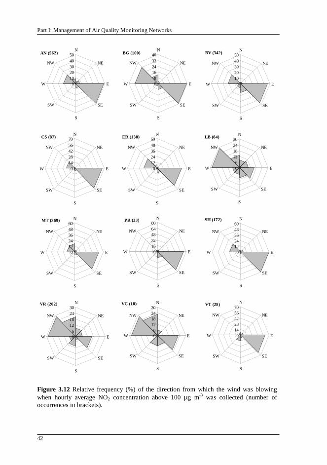
Part I: Management of Air Quality Monitoring Networks
42
AN (562)
01020304050
N
NE
E
SE
S
SW
W
NW
BG (100)
08
16243240
N
NE
E
SE
S
SW
W
NW
BV (342)
01020304050
N
NE
E
SE
S
SW
W
NW
CS (87)
01428425670
N
NE
E
SE
S
SW
W
NW
ER (138)
01224364860
N
NE
E
SE
S
SW
W
NW
LB (84)
06
12182430
N
NE
E
SE
S
SW
W
NW
MT (369)
01224364860
N
NE
E
SE
S
SW
W
NW
PR (33)
01632486480
N
NE
E
SE
S
SW
W
NW
SH (172)
01224364860
N
NE
E
SE
S
SW
W
NW
VR (202)
06
12182430
N
NE
E
SE
S
SW
W
NW
VC (18)
06
12182430
N
NE
E
SE
S
SW
W
NW
VT (28)
01428425670
N
NE
E
SE
S
SW
W
NW
Figure 3.12 Relative frequency (%) of the direction from which the wind was blowing when hourly average NO2 concentration above 100 µg m-3 was collected (number of occurrences in brackets).
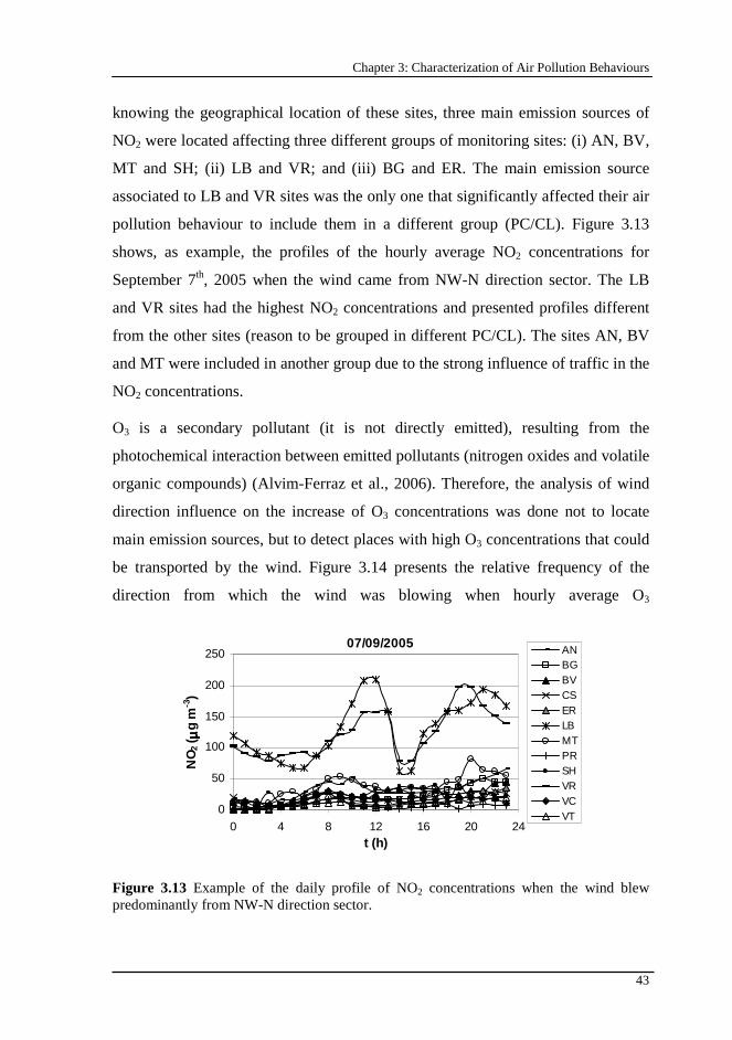
Chapter 3: Characterization of Air Pollution Behaviours
43
knowing the geographical location of these sites, three main emission sources of
NO2 were located affecting three different groups of monitoring sites: (i) AN, BV,
MT and SH; (ii) LB and VR; and (iii) BG and ER. The main emission source
associated to LB and VR sites was the only one that significantly affected their air
pollution behaviour to include them in a different group (PC/CL). Figure 3.13
shows, as example, the profiles of the hourly average NO2 concentrations for
September 7th, 2005 when the wind came from NW-N direction sector. The LB
and VR sites had the highest NO2 concentrations and presented profiles different
from the other sites (reason to be grouped in different PC/CL). The sites AN, BV
and MT were included in another group due to the strong influence of traffic in the
NO2 concentrations.
O3 is a secondary pollutant (it is not directly emitted), resulting from the
photochemical interaction between emitted pollutants (nitrogen oxides and volatile
organic compounds) (Alvim-Ferraz et al., 2006). Therefore, the analysis of wind
direction influence on the increase of O3 concentrations was done not to locate
main emission sources, but to detect places with high O3 concentrations that could
be transported by the wind. Figure 3.14 presents the relative frequency of the
direction from which the wind was blowing when hourly average O3
07/09/2005
0
50
100
150
200
250
0 4 8 12 16 20 24t (h)
NO
2 (µµ µµ
g m
-3)
ANBGBVCSERLBMTPRSHVRVCVT
Figure 3.13 Example of the daily profile of NO2 concentrations when the wind blew predominantly from NW-N direction sector.
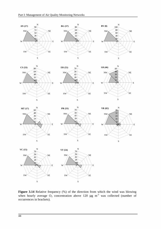
Part I: Management of Air Quality Monitoring Networks
44
AN (27)
01836547290
N
NE
E
SE
S
SW
W
NW
BG (37)
01632486480
N
NE
E
SE
S
SW
W
NW
BV (8)
020406080
100N
NE
E
SE
S
SW
W
NW
CS (33)
01632486480
N
NE
E
SE
S
SW
W
NW
ER (55)
01428425670
N
NE
E
SE
S
SW
W
NW
LB (46)
01224364860
N
NE
E
SE
S
SW
W
NW
MT (17)
01224364860
N
NE
E
SE
S
SW
W
NW
PR (33)
01428425670
N
NE
E
SE
S
SW
W
NW
VR (82)
08
16243240
N
NE
E
SE
S
SW
W
NW
VC (15)
01428425670
N
NE
E
SE
S
SW
W
NW
VT (54)
01428425670
N
NE
E
SE
S
SW
W
NW
Figure 3.14 Relative frequency (%) of the direction from which the wind was blowing when hourly average O3 concentration above 120 µg m-3 was collected (number of occurrences in brackets).
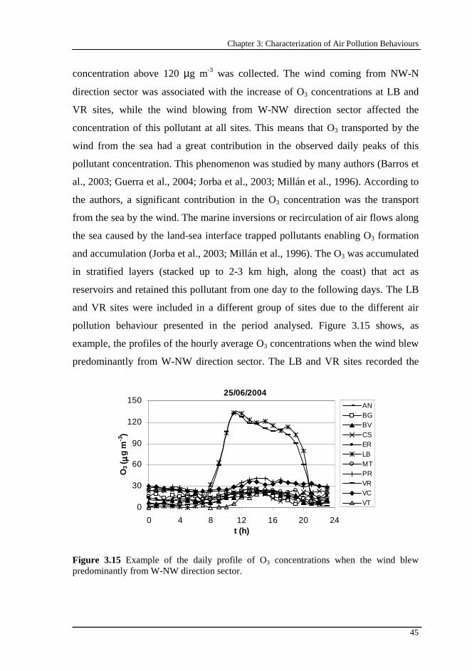
Chapter 3: Characterization of Air Pollution Behaviours
45
concentration above 120 µg m-3 was collected. The wind coming from NW-N
direction sector was associated with the increase of O3 concentrations at LB and
VR sites, while the wind blowing from W-NW direction sector affected the
concentration of this pollutant at all sites. This means that O3 transported by the
wind from the sea had a great contribution in the observed daily peaks of this
pollutant concentration. This phenomenon was studied by many authors (Barros et
al., 2003; Guerra et al., 2004; Jorba et al., 2003; Millán et al., 1996). According to
the authors, a significant contribution in the O3 concentration was the transport
from the sea by the wind. The marine inversions or recirculation of air flows along
the sea caused by the land-sea interface trapped pollutants enabling O3 formation
and accumulation (Jorba et al., 2003; Millán et al., 1996). The O3 was accumulated
in stratified layers (stacked up to 2-3 km high, along the coast) that act as
reservoirs and retained this pollutant from one day to the following days. The LB
and VR sites were included in a different group of sites due to the different air
pollution behaviour presented in the period analysed. Figure 3.15 shows, as
example, the profiles of the hourly average O3 concentrations when the wind blew
predominantly from W-NW direction sector. The LB and VR sites recorded the
25/06/2004
0
30
60
90
120
150
0 4 8 12 16 20 24t (h)
O3 (
µµ µµg
m-3
)
ANBGBVCSERLBMTPRVRVCVT
Figure 3.15 Example of the daily profile of O3 concentrations when the wind blew predominantly from W-NW direction sector.
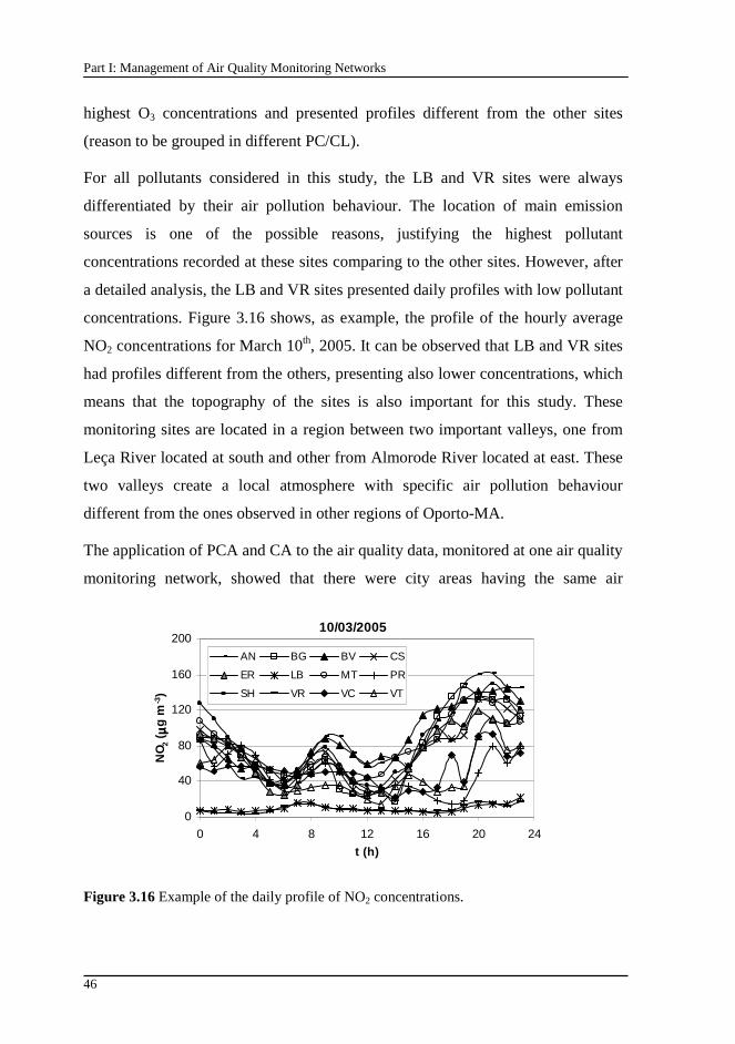
Part I: Management of Air Quality Monitoring Networks
46
highest O3 concentrations and presented profiles different from the other sites
(reason to be grouped in different PC/CL).
For all pollutants considered in this study, the LB and VR sites were always
differentiated by their air pollution behaviour. The location of main emission
sources is one of the possible reasons, justifying the highest pollutant
concentrations recorded at these sites comparing to the other sites. However, after
a detailed analysis, the LB and VR sites presented daily profiles with low pollutant
concentrations. Figure 3.16 shows, as example, the profile of the hourly average
NO2 concentrations for March 10th, 2005. It can be observed that LB and VR sites
had profiles different from the others, presenting also lower concentrations, which
means that the topography of the sites is also important for this study. These
monitoring sites are located in a region between two important valleys, one from
Leça River located at south and other from Almorode River located at east. These
two valleys create a local atmosphere with specific air pollution behaviour
different from the ones observed in other regions of Oporto-MA.
The application of PCA and CA to the air quality data, monitored at one air quality
monitoring network, showed that there were city areas having the same air
10/03/2005
0
40
80
120
160
200
0 4 8 12 16 20 24
t (h)
NO
2 ( µµ µµ
g m
-3)
AN BG BV CS
ER LB MT PR
SH VR VC VT
Figure 3.16 Example of the daily profile of NO2 concentrations.
Chapter 3: Characterization of Air Pollution Behaviours
47
pollution behaviour covered by too many monitoring sites; suggesting that
monitoring network can be better managed. This means that PCA and CA have a
great potential for the management of air quality monitoring systems, helping the
identification of redundant equipment that might be transferred to other sites
allowing an enlargement of the monitored area.
3.4. Conclusions
Aiming the identification of city areas with similar air pollution behaviours in
Oporto-MA, two statistical methods, PCA and CA, were applied. Different results
were obtained for each pollutant. PCA and CA divided the sites in: (i) six different
groups for SO2; (ii) three groups for CO and for NO2; and (iii) two groups for
PM10 and O3.
The number of site groups with similar pollution behaviour was affected by the
geographic location of the emission sources. Approximate source locations were
found through the analysis of the information contained in the wind direction
sectors associated to the presence of high concentrations of the analysed air
pollutants. Only one main source of SO2 was identified, being located inside the
region covered by the AQMN. For each wind direction, the daily evolution of SO2
concentrations was not the same at all monitoring sites; this means that the sites
can be grouped according to this specific behaviour. Results showed that six
monitoring sites were needed to characterize SO2 concentrations. Three main
emission sources of PM10 were located: (i) one inside the region defined by the
AQMN (significantly affected only two sites) and (ii) two outside that region
(affecting all monitoring sites). One emission source located outside the region
affected significantly only one monitoring site in a short period of the day. This
emission source decreased its impact in 2005. Therefore, only two monitoring sites
are needed to characterize PM10 concentrations. Additionally, four main emission
sources of CO and NO2 were located. Additionally, it was observed that sea wind

Part I: Management of Air Quality Monitoring Networks
48
had an important contribution in the increase of the O3 concentration due to the O3
accumulation above the sea.
Two monitoring sites presented different air pollution behaviour for all pollutants
during the analysed period. This difference was related with the location of main
emission sources and also with the topography of the region where these sites are
located.
49
Chapter 4
4. Identification of redundant air quality measurements
This chapter shows the results obtained by principal component analysis in the identification of redundant measurements using two different criteria for selection of the number of principal components. For each air pollutant, the minimum number of monitoring sites evaluated by this analysis was compared to what was established by the European Union legislation. To validate the results, the statistical models were determined to estimate air pollutant concentrations at removed monitoring sites using the concentrations measured at the remaining monitoring sites. These models were tested in a year’s data.
The contents of this chapter were adapted from: (i) Pires, J.C.M., Pereira, M.C., Alvim-Ferraz, M.C.M., Martins, F.G., 2009. Identification of redundant air quality measurements through the use of principal component analysis. Atmospheric Environment 43, 3837-3842.
4.1. Introduction
The concerns about the negative effects of air pollution led to increased efforts to
prevent and control this phenomenon. The location of sampling points for the
measurement of air pollutant concentrations was defined by the European Union
directive 2008/50/EC (EC Directive, 2008). According to this directive,
monitoring sites should be placed to provide data: (i) in areas within zones and
agglomerations, where the population is likely to be directly or indirectly exposed
to high concentrations (limit and target values were established as references); (ii)
in other areas within zones and agglomerations which are representative of the
general population exposure. The same directive defined the number of monitoring
sites that should operate according to population size and pollution levels. In
Part I: Management of Air Quality Monitoring Networks
50
Oporto Metropolitan Area (Oporto-MA) with population of about 1.7 millions and
a population density of 540 inhabitants per square kilometre, NO2 and PM10
concentrations exceeded many times the limits established by the legislation (see
Chapter 2). Five monitoring sites should operate (including at least an urban
background site and a traffic site) to measure NO2 and PM10 concentrations and
three monitoring sites should measure the O3 concentrations (at least 50% of the
monitoring sites should be placed in suburban areas).
In Chapter 3, PCA and CA were applied to identify the monitoring sites with
similar air pollution behaviour and to locate emission sources of SO2, PM10, CO,
NO2 and O3. However, this study was performed using all period of study, not
considering the annual variations of the air pollutant behaviours due to the
different meteorological conditions. In this study, PCA was applied to the data
divided into annual quarters. Moreover, an additional criterion for selection of the
number of PCs was applied, aiming to select PCs containing more information
about the original data than the criterion usually applied (Kaiser criterion) and the
number of monitoring sites was compared with what was established by the
legislation. Finally, after the selection of the monitoring sites that should operate,
the air pollutant concentrations measured in these locations were used to predict
the concentrations at the removed monitoring sites.
4.2. Air quality data
The monitoring sites considered in this study were Antas (AN), Boavista (BV),
Custóias (CS), Leça do Balio (LB), Matosinhos (MT), Perafita (PR), Vermoim
(VR), Vila do Conde (VC) and Vila Nova da Telha (VT). Their location, type and
main characteristics are presented in Chapter 2. Oporto monitoring network
includes other monitoring sites that were not considered in this study: some did not
measure all the considered air pollutants (Baguim and Senhora da Hora) and
others presented a high percentage of missing data during the analysed period
(Ermesinde and Espinho). The pollutants considered were NO2, PM10 and O3,
Chapter 4: Identification of redundant air quality measurements
51
since CO and SO2 did not present a significant number of exceedances to the
limits established by the European Union for the protection of human health
during the analysed period (Pires et al., 2008a, 2008b).
The analysed period was from January 2003 to December 2005. PCA was applied
to the data corresponding to the first two years that were divided in eight annual
quarters (Qi). The division into annual quarters had the objective of analyse the
persistence of the PCA results during the year. The annual analysis can hide
seasonal changes, i.e., variability of the meteorological conditions. The last year
was used to validate the results of PCA. After the selection of the monitoring sites
that should be removed or replaced, the air pollutant concentrations at these places
were estimated using the values measured at the remaining monitoring sites. The
data were organized in such a way that each column had the hourly average
concentrations of a specific air pollutant at a specific monitoring site. To be
possible to apply the PCA, the air pollutant concentrations must be available at the
same time in all monitoring sites. The data available for the analysis in 2003, 2004
and 2005 were, respectively: (i) 4897, 3532 and 4755 for NO2; (ii) 4737, 4408 and
5869 for O3; and (iii) 2534, 7492 and 1951 for PM10. Concentrations were Z
standardized to have zero mean and unit standard deviation.
4.3. Results and discussion
PCA was applied as a classification method to group monitoring sites with
redundant measurements of air pollutant concentrations during the analysed
period. The first step of PCA is the selection of the number of PCs. Kaiser
criterion, which selects PCs with eigenvalues greater than 1, is commonly used for
this purpose (Yidana et al., 2008); as this criterion does not usually achieve 90%
of the original data variance (Mendiguchía et al., 2004; Pires et al., 2008a, 2008b),
in this study, a different criterion was also used, aiming to select PCs representing
at least 90% of the original data variance (ODV90); this procedure allowed to
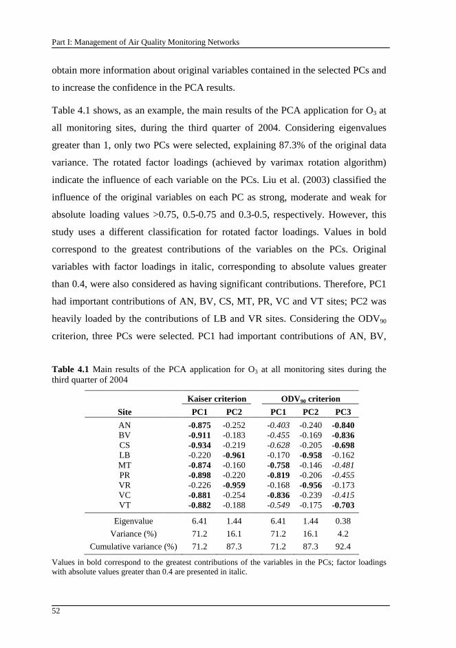
Part I: Management of Air Quality Monitoring Networks
52
obtain more information about original variables contained in the selected PCs and
to increase the confidence in the PCA results.
Table 4.1 shows, as an example, the main results of the PCA application for O3 at
all monitoring sites, during the third quarter of 2004. Considering eigenvalues
greater than 1, only two PCs were selected, explaining 87.3% of the original data
variance. The rotated factor loadings (achieved by varimax rotation algorithm)
indicate the influence of each variable on the PCs. Liu et al. (2003) classified the
influence of the original variables on each PC as strong, moderate and weak for
absolute loading values >0.75, 0.5-0.75 and 0.3-0.5, respectively. However, this
study uses a different classification for rotated factor loadings. Values in bold
correspond to the greatest contributions of the variables on the PCs. Original
variables with factor loadings in italic, corresponding to absolute values greater
than 0.4, were also considered as having significant contributions. Therefore, PC1
had important contributions of AN, BV, CS, MT, PR, VC and VT sites; PC2 was
heavily loaded by the contributions of LB and VR sites. Considering the ODV90
criterion, three PCs were selected. PC1 had important contributions of AN, BV,
Table 4.1 Main results of the PCA application for O3 at all monitoring sites during the third quarter of 2004
Kaiser criterion ODV90 criterion
Site PC1 PC2 PC1 PC2 PC3
AN -0.875 -0.252 -0.403 -0.240 -0.840 BV -0.911 -0.183 -0.455 -0.169 -0.836 CS -0.934 -0.219 -0.628 -0.205 -0.698 LB -0.220 -0.961 -0.170 -0.958 -0.162 MT -0.874 -0.160 -0.758 -0.146 -0.481 PR -0.898 -0.220 -0.819 -0.206 -0.455 VR -0.226 -0.959 -0.168 -0.956 -0.173 VC -0.881 -0.254 -0.836 -0.239 -0.415 VT -0.882 -0.188 -0.549 -0.175 -0.703
Eigenvalue 6.41 1.44 6.41 1.44 0.38
Variance (%) 71.2 16.1 71.2 16.1 4.2
Cumulative variance (%) 71.2 87.3 71.2 87.3 92.4
Values in bold correspond to the greatest contributions of the variables in the PCs; factor loadings with absolute values greater than 0.4 are presented in italic.
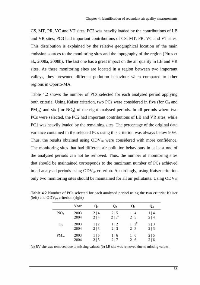
Chapter 4: Identification of redundant air quality measurements
53
CS, MT, PR, VC and VT sites; PC2 was heavily loaded by the contributions of LB
and VR sites; PC3 had important contributions of CS, MT, PR, VC and VT sites.
This distribution is explained by the relative geographical location of the main
emission sources to the monitoring sites and the topography of the region (Pires et
al., 2008a, 2008b). The last one has a great impact on the air quality in LB and VR
sites. As these monitoring sites are located in a region between two important
valleys, they presented different pollution behaviour when compared to other
regions in Oporto-MA.
Table 4.2 shows the number of PCs selected for each analysed period applying
both criteria. Using Kaiser criterion, two PCs were considered in five (for O3 and
PM10) and six (for NO2) of the eight analysed periods. In all periods where two
PCs were selected, the PC2 had important contributions of LB and VR sites, while
PC1 was heavily loaded by the remaining sites. The percentage of the original data
variance contained in the selected PCs using this criterion was always below 90%.
Thus, the results obtained using ODV90 were considered with more confidence.
The monitoring sites that had different air pollution behaviours in at least one of
the analysed periods can not be removed. Thus, the number of monitoring sites
that should be maintained corresponds to the maximum number of PCs achieved
in all analysed periods using ODV90 criterion. Accordingly, using Kaiser criterion
only two monitoring sites should be maintained for all air pollutants. Using ODV90
Table 4.2 Number of PCs selected for each analysed period using the two criteria: Kaiser (left) and ODV90 criterion (right)
Year Q1 Q2 Q3 Q4
NO2 2003 2 | 4 2 | 5 1 | 4 1 | 4 2004 2 | 4 2 | 5a 2 | 5 2 | 4
O3 2003 1 | 2 1 | 2 1 | 2b 2 | 3 2004 2 | 3 2 | 3 2 | 3 2 | 3
PM10 2003 1 | 5 1 | 6 1 | 6 2 | 5 2004 2 | 5 2 | 7 2 | 6 2 | 6
(a) BV site was removed due to missing values; (b) LB site was removed due to missing values.
Part I: Management of Air Quality Monitoring Networks
54
criterion, the number of monitoring sites needed to characterize the region was: (i)
five for NO2; (ii) three for O3; and (iii) seven for PM10. Using the last criterion, the
number of monitoring sites for NO2 and O3 was in agreement with what was
established by the legislation. However, for PM10, Oporto-MA needed two more
monitoring sites.
The sites to be maintained should be selected according to the following criteria:
(i) sites should be representative, namely for monitoring of the highest pollutant
concentrations; (ii) the number of pollutants being monitored at each site should
be maximized; and (iii) the distribution should maximize distances between
monitoring sites. Table 4.3 shows the relative frequency (in percentage) of each
pair of monitoring sites that had important contributions in the same PC during the
eight analysed periods (training period) using Kaiser (upper triangular matrix) and
ODV90 criteria (lower triangular matrix). High frequencies (values in bold) means
that the correspondent pair of monitoring sites often presented redundant
measurements. Based on this information, the monitoring sites that presented high
redundancy in the data were identified. The selection of the monitoring sites to be
maintained or removed was performed considering the frequencies presented in
Table 4.3 and the criteria referred above. Accordingly, considering Kaiser
criterion, only two monitoring sites should be maintained for all analysed air
pollutants. The selected monitoring sites were BV and LB. Considering ODV90
criterion, the sites that should be removed are: CS and VR for PM10; CS, VR, AN
and VT for NO2; and CS, VR, AN, VT, MT and PR for O3.
To validate the PCA results, air pollutant concentrations at the removed
monitoring sites were estimated through statistical models using the values
measured at other places in Oporto-MA. The performance of these models was
evaluated using the data of the last year of the study period. Multiple linear
regression (MLR) was applied with this aim and the input variables were selected
according to Table 4.3. For example, NO2 concentrations at CS site can be
estimated using the NO2 concentrations measured at BV if Kaiser criterion was
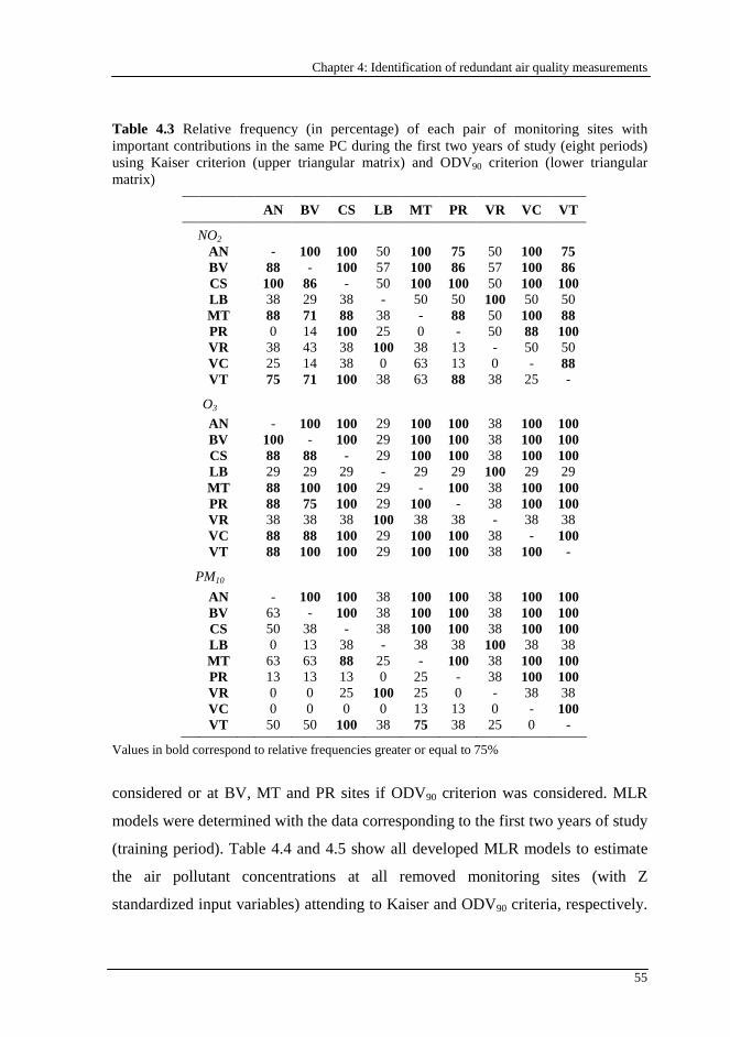
Chapter 4: Identification of redundant air quality measurements
55
Table 4.3 Relative frequency (in percentage) of each pair of monitoring sites with important contributions in the same PC during the first two years of study (eight periods) using Kaiser criterion (upper triangular matrix) and ODV90 criterion (lower triangular matrix)
AN BV CS LB MT PR VR VC VT
NO2 AN - 100 100 50 100 75 50 100 75 BV 88 - 100 57 100 86 57 100 86 CS 100 86 - 50 100 100 50 100 100 LB 38 29 38 - 50 50 100 50 50 MT 88 71 88 38 - 88 50 100 88 PR 0 14 100 25 0 - 50 88 100 VR 38 43 38 100 38 13 - 50 50 VC 25 14 38 0 63 13 0 - 88 VT 75 71 100 38 63 88 38 25 -
O3
AN - 100 100 29 100 100 38 100 100 BV 100 - 100 29 100 100 38 100 100 CS 88 88 - 29 100 100 38 100 100 LB 29 29 29 - 29 29 100 29 29 MT 88 100 100 29 - 100 38 100 100 PR 88 75 100 29 100 - 38 100 100 VR 38 38 38 100 38 38 - 38 38 VC 88 88 100 29 100 100 38 - 100 VT 88 100 100 29 100 100 38 100 -
PM10
AN - 100 100 38 100 100 38 100 100 BV 63 - 100 38 100 100 38 100 100 CS 50 38 - 38 100 100 38 100 100 LB 0 13 38 - 38 38 100 38 38 MT 63 63 88 25 - 100 38 100 100 PR 13 13 13 0 25 - 38 100 100 VR 0 0 25 100 25 0 - 38 38 VC 0 0 0 0 13 13 0 - 100 VT 50 50 100 38 75 38 25 0 -
Values in bold correspond to relative frequencies greater or equal to 75%
considered or at BV, MT and PR sites if ODV90 criterion was considered. MLR
models were determined with the data corresponding to the first two years of study
(training period). Table 4.4 and 4.5 show all developed MLR models to estimate
the air pollutant concentrations at all removed monitoring sites (with Z
standardized input variables) attending to Kaiser and ODV90 criteria, respectively.
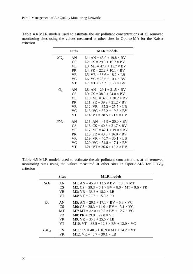
Part I: Management of Air Quality Monitoring Networks
56
Table 4.4 MLR models used to estimate the air pollutant concentrations at all removed monitoring sites using the values measured at other sites in Oporto-MA for the Kaiser criterion
Sites MLR models
NO2 AN L1: AN = 45.9 + 19.8 × BV CS L2: CS = 29.3 + 15.7 × BV MT L3: MT = 47.7 + 15.7 × BV PR L4: PR = 22.2 + 10.1 × BV VR L5: VR = 33.6 + 18.2 × LB VC L6: VC = 28.5 + 10.4 × BV VT L7: VT = 22.7 + 13.2 × BV
O3 AN L8: AN = 29.1 + 21.5 × BV CS L9: CS = 38.3 + 24.0 × BV MT L10: MT = 32.0 + 20.2 × BV PR L11: PR = 39.9 + 21.2 × BV VR L12: VR = 35.3 + 25.5 × LB VC L13: VC = 35.2 + 19.3 × BV VT L14: VT = 38.5 + 21.5 × BV
PM10 AN L15: AN = 45.9 + 20.0 × BV CS L16: CS = 40.3 + 21.7 × BV MT L17: MT = 42.1 + 19.0 × BV PR L18: PR = 43.9 + 16.0 × BV VR L19: VR = 40.7 + 30.1 × LB VC L20: VC = 54.8 + 17.1 × BV VT L21: VT = 36.6 + 15.3 × BV
Table 4.5 MLR models used to estimate the air pollutant concentrations at all removed monitoring sites using the values measured at other sites in Oporto-MA for ODV90 criterion
Sites MLR models
NO2 AN M1: AN = 45.9 + 13.5 × BV + 10.5 × MT CS M2: CS = 29.3 + 6.1 × BV + 8.0 × MT + 9.6 × PR VR M3: VR = 33.6 + 18.2 × LB VT M4: VT = 22.7 + 15.9 × PR
O3 AN M5: AN = 29.1 + 17.1 × BV + 5.8 × VC CS M6: CS = 38.3 + 14.0 × BV + 13.1 × VC MT M7: MT = 32.0 +10.5 × BV + 12.7 × VC PR M8: PR = 39.9 + 22.8 × VC VR M9: VR = 35.3 + 25.5 × LB VT M10: VT = 38.5 + 12.3 × BV + 12.0 × VC
PM10 CS M11: CS = 40.3 + 16.9 × MT + 14.2 × VT VR M12: VR = 40.7 + 30.1 × LB
Chapter 4: Identification of redundant air quality measurements
57
The data corresponding to the last year of study were used to evaluate the
performance of MLR models. The performance indexes used in this study were the
Pearson correlation coefficient (R) and the index of agreement of second order
(d2). Figure 4.1 and 4.2 show the performance indexes of all MLR models in the
(a) training and (b) test periods for Kaiser and ODV90 criteria, respectively. The
models achieved with ODV90 criterion presented better performances. Considering
this criterion, all models achieved good performances, which mean that the
monitoring sites proposed by PCA were enough to infer the air pollutant
concentrations at all monitored region. The air pollutant analysers corresponding
to the redundant measurements can be installed in non-monitored regions,
allowing the enlargement of the air quality monitoring network.
4.4. Conclusions
This study aims to apply PCA to evaluate redundant measurements in the air
quality monitoring network of Oporto-MA. PCA was used to group the monitoring
sites with redundant measurements. Two different criteria were used for selection
of the number of PCs. ODV90 criterion had always more information about the
original variables when compared with Kaiser criterion. According to the PCA
results with ODV90 criterion, only five monitoring sites for NO2, three for O3 and
seven for PM10 were needed to characterize the region. The number of monitoring
sites for NO2 and O3 was in agreement with what was established by the
legislation. However, for PM10, Oporto-MA needed two more monitoring sites. To
validate PCA results, MLR models were determined to estimate air pollutant
concentrations at removed monitoring sites using the concentrations measured in
the remaining monitoring sites. These models were applied to a year’s data. The
good performance obtained by the models showed that the monitoring sites
selected by the procedure presented in this study were enough to infer the air
pollutant concentrations in the region defined by the initial monitoring sites.
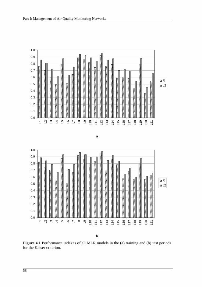
Part I: Management of Air Quality Monitoring Networks
58
0.0
0.1
0.2
0.3
0.4
0.5
0.6
0.7
0.8
0.9
1.0
L1 L2 L3 L4 L5 L6 L7 L8 L9 L10
L11
L12
L13
L14
L15
L16
L17
L18
L19
L20
L21
R
d2
a
0.0
0.1
0.2
0.3
0.4
0.5
0.6
0.7
0.8
0.9
1.0
L1 L2 L3 L4 L5 L6 L7 L8 L9 L10
L11
L12
L13
L14
L15
L16
L17
L18
L19
L20
L21
R
d2
b
Figure 4.1 Performance indexes of all MLR models in the (a) training and (b) test periods for the Kaiser criterion.
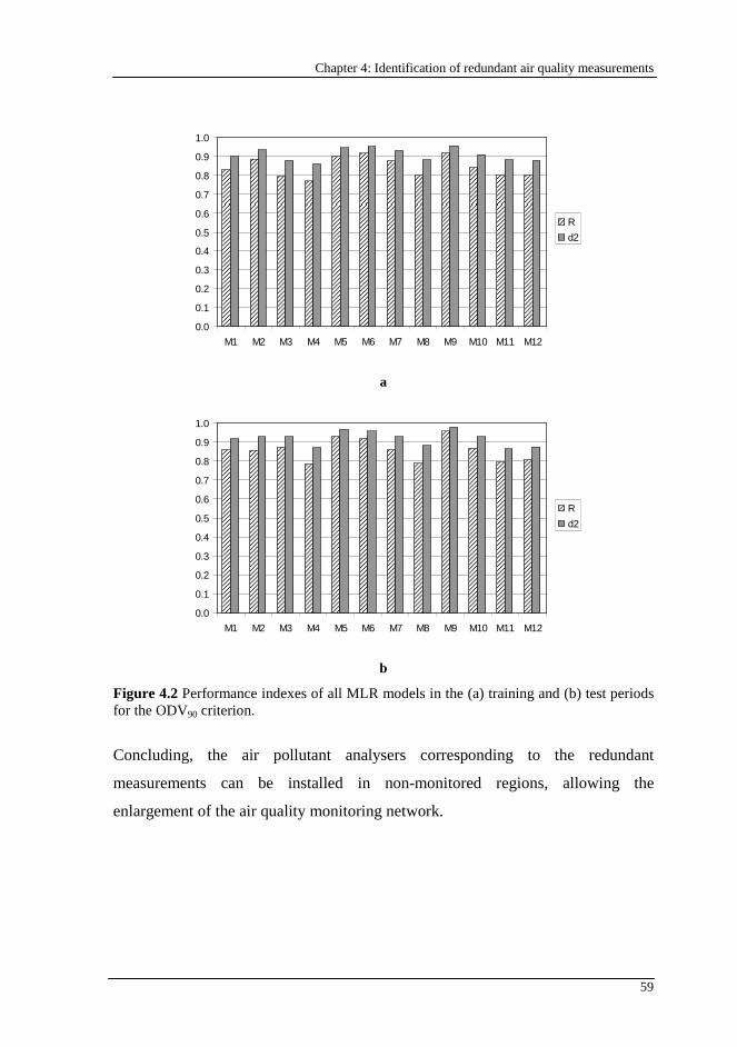
Chapter 4: Identification of redundant air quality measurements
59
0.0
0.1
0.2
0.3
0.4
0.5
0.6
0.7
0.8
0.9
1.0
M1 M2 M3 M4 M5 M6 M7 M8 M9 M10 M11 M12
R
d2
a
0.0
0.1
0.2
0.3
0.4
0.5
0.6
0.7
0.8
0.9
1.0
M1 M2 M3 M4 M5 M6 M7 M8 M9 M10 M11 M12
R
d2
b
Figure 4.2 Performance indexes of all MLR models in the (a) training and (b) test periods for the ODV90 criterion.
Concluding, the air pollutant analysers corresponding to the redundant
measurements can be installed in non-monitored regions, allowing the
enlargement of the air quality monitoring network.

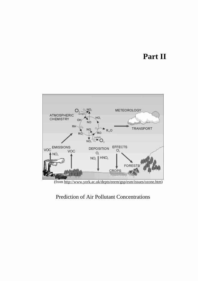
Part II
(from http://www.york.ac.uk/depts/eeem/gsp/esm/issues/ozone.htm)
Prediction of Air Pollutant Concentrations

63
Chapter 5
5. Prediction using statistical models
In last years, several statistical models were tested aiming the prediction of O3 and PM10 concentrations. This chapter describes some of these studies. Additionally, the models applied in this thesis were briefly presented.
5.1. State of the art
Several studies can be found in literature aiming the prediction of O3 and PM10
concentrations through statistical models. Prybutok et al. (2000) predicted the
daily maximum O3 concentrations using artificial neural networks (ANNs),
multiple linear regression and autoregressive integrated moving average (ARIMA)
models. The ANN model presented better performance.
Schlink et al. (2003) applied 15 different statistical techniques for ozone
forecasting using ten data sets. This study was the only one found in the literature
that applied artificial neural network quantile regression to the environmental
field. However, the artificial neural network was determined using only the
median regression and not taken into account all potentialities of the quantile
regression.
Wang et al. (2003) developed an ANN model, which combines the adaptive radial
basis function network with statistical characteristics of O3 in selected specific
areas, and is used to predict the daily maximum O3 concentrations. The model was
capable to predict successfully the daily maximum concentrations.
Part II: Prediction of Air Pollutant Concentrations
64
Baur et al. (2004) applied the linear quatile regression (QR) for the interpretation
of nonlinear relationships between daily maximum hourly average ozone
concentrations and meteorological variables. This study showed that the
contributions of the explanatory variables in the O3 concentrations vary
significantly at different O3 regimes. Additionally, linear QR model (with five
quantiles) was compared with ordinary least-squares regression models in the
prediction of O3 concentrations presenting better performance indexes.
Heo and Kim (2004) tried to predict daily maximum O3 concentrations at four
monitoring sites using a fuzzy expert and ANN models. The developed models
were able to correct themselves and presented reduced forecasting errors.
Dueñas et al. (2005) developed stochastic models, such as ARIMA, for urban and
rural areas that turned out to be site specific. In both sampling points, predictions
of hourly ozone concentrations agree reasonably well with measured values.
Sousa et al. (2006) compared the performances of multiple linear regression
(MLR), feedforward ANN and time series in the prediction of the daily average O3
concentrations. These models were also applied to urban and rural sites. MLR
models showed good performance in the training step, but ANN presented better
predictive performance.
Sousa et al. (2007) predicted next day hourly average O3 concentrations through a
new methodology based on feedforward ANNs using principal components as
inputs. The performance of this model was compared with other approach on
neural networks and with a linear model. The results showed that ANNs predict
better than linear models.
Sousa et al. (2009) also compared MLR and QR approach for the prediction of the
next day hourly average O3 concentrations. Three different periods were applied:
daylight, night time and all day. QR allowed more efficient previsions of extreme
values which are very useful once the forecasting of higher concentrations is
fundamental to develop strategies for protecting the public health.
Chapter 5: Prediction using statistical models
65
Concerning the prediction of PM10 concentrations, Fuller et al. (2002) used an
empirical model to forecast the concentrations of PM10 at background and roadside
locations. The method was based on the regression analysis between PM10 and
NOx. The model accurately predicted daily mean PM10 concentrations but
presented some limitations. For example, it depended of the existence of a
consistent relationship between PM10 and NOx emissions. As a conclusion of these
studies, it was noted that the comparisons between linear and nonlinear models did
not find significant differences in the results obtained by the different
methodologies.
Perez and Reyes (2002) developed a neural network (nonlinear approach) to
predict the maximum of the 24 h moving average of PM10 concentration on the
next day. This method was compared with linear perceptron (linear approach) and
presented slightly better performance.
Kukkonen et al. (2003) applied five ANN models, a linear statistical model and a
deterministic modelling system for the prediction of urban NO2 and PM10
concentrations. For both pollutants, ANN models presented better results than the
other models.
Corani (2005) tried to predict this pollutant using feedforward ANNs, pruned
neural networks (nonlinear approaches) and lazy learning (local linear modelling
approach). Comparing these three methodologies, lazy learning presents slightly
better results than the other methods.
Slini et al. (2006) applied classification and regression trees and ANN to forecast
PM10 concentrations trends. Both methods presented good results, having the first
one the best performance indexes.
Grivas and Chaloulakou (2006) applied ANN models to predict hourly average
PM10 concentrations. The input variables were selected using a genetic algorithm
procedure. The performance of these models was better than the one presented by
MLR.
Part II: Prediction of Air Pollutant Concentrations
66
5.2. Models applied in this thesis
This thesis presented the development and application of some statistical models
(linear and nonlinear) to predict the next day hourly average O3 concentrations and
the daily average PM10 concentrations in urban areas. The linear models applied
with this aim were: (i) MLR; (ii) principal component regression (PCR); (iii)
independent component regression (ICR); (iv) partial least squares regression
(PLSR); and (v) QR. As far as it is known, no study had applied ICR for the
prediction of O3 or PM10 concentrations. Moreover, a method was presented to
estimate the percentile of the predicted variable in QR. Considering the artificial
neural networks, two step-by-step methodologies were applied to define these
models, taking into account some limitations of these models. The last models are
related to evolutionary algorithms. Genetic algorithms were applied to define
threshold regression models to predict O3 concentrations. Finally, genetic
programming and multi-gene genetic programming were applied to predict O3 and
PM10 concentrations, respectively.
67
Chapter 6
6. Linear models
This chapter has the objective of evaluate the performance of five linear regression models in the prediction of the next day hourly average O3 concentrations and the daily average PM10 concentrations. The selected models were: (i) multiple linear regression; (ii) principal component regression; (iii) independent component regression; (iv) partial least squares regression; and (v) quantile regression. The predictors were meteorological data (hourly/daily averages of temperature, relative humidity and wind speed) and environmental data (hourly/daily average concentrations of SO2, CO, NO, NO2, O3 and PM10) of the previous day collected in an urban site with traffic influences.
The contents of this chapter were adapted from: (i) Pires, J.C.M., Martins, F.G., Sousa, S.I.V., Alvim-Ferraz, M.C.M., Pereira, M.C., 2008. Prediction of the Daily Mean PM10 Concentrations Using Linear Models. American Journal of Environmental Sciences 4 (5), 445-453; and (ii) Pires, J.C.M., Martins, F.G., Alvim-Ferraz, M.C.M., Pereira, M.C., 2009. Comparison of several statistical models to predict O3 concentrations. Submitted for publication.
6.1. Multiple linear regression
Multiple linear regression (MLR) is an extension of the simple linear regression
model for data with multiple predictor variables and one outcome. Thus, this
statistical model assumes that the best approach to estimate the dependent variable
y from the explanatory variables X is to find the linear combination of these
variables that minimizes the errors in reproducing y. This relationship is given by:
eXby += (6.1)
Part II: Prediction of Air Pollutant Concentrations
68
where b is the vector of the regression parameters and e is the vector of the errors
associated to MLR model, which are normally distributed with zero mean and
constant variance σ2 (Agirre-Basurko et al., 2006; Pires et al, 2008c). A common
method for estimating the regression parameters is the ordinary least squares. This
method obtains the parameters’ estimates by minimizing the sum of the squared
errors (SSE). The least squares estimate of b is given by:
( ) yXXXb T1T −= (6.2)
where the superscripts T and -1 refer to the transpose and inverse matrix operations,
respectively.
Collinearity is a serious problem of MLR, which means the redundancy in the set
of the variables, i.e., the predictors are correlated to each other. It has several
consequences: (i) problems in the determination of the regression parameters; and
(ii) wrong interpretations of the achieved models (Pires et al., 2008c). The
regression parameters are obtained through the Equation 6.2, depending on the
inverse of the matrix product. If a strong collinearity exists, this product is singular
(Sundberg, 2000). Thus, it does not have a unique inverse and, consequently, there
is infinity of solutions for the regression parameters. Moreover, in the presence of
collinearity, the standard errors of the regression parameters tend to be large and,
consequently, their confidence intervals tend to be very wide. In that case, the test
of the hypothesis that the regression parameter is equal to zero against the
alternative that it is not equal to zero leads to a failure to reject the null hypothesis
(Eberly, 2007). Thus, this regression parameter is considered statistically
insignificant and no linear relationship is established between the dependent and
the independent variable. Additionally, as the confidence intervals are so wide,
excluding a variable (or adding a new one) can change the regression parameters
dramatically. Thus, magnitudes and possible directions (signs) of the regression
parameters may change depending on which predictors are included in the model.
Chapter 6: Linear Models
69
For this reason, it is always good to verify if the magnitude and a direction of the
regression parameter has meaning in the context of the study (Pires et al., 2008c).
In this study, two statistical methods were applied to remove the collinearity
between the explanatory variables: (i) principal component analysis (PCA); and
(ii) independent component analysis (ICA). The variables created by these linear
transformations, called principal components (PCs) and independent components
(ICs), are uncorrelated to each other.
6.2. Principal component regression
Principal component analysis (PCA) is mathematically defined as an orthogonal
linear transformation that modifies the original data to a new coordinate system
such that the greatest variance by any projection of the data comes to lie on the
first coordinate (called the first principal component), the second greatest variance
on the second coordinate, and so on (Pires et al., 2008a, 2008b). Thus, the PCs are
orthogonal and uncorrelated to each other, being determined by linear
combinations of the original variables. The directions of the new coordinate axes
are given by the eigenvectors of the covariance matrix of the original variables.
The magnitude of the eigenvalues corresponds to the variance of the data along the
eigenvector direction.
PCs are dependent on the units used to measure the original variables as well as on
the range of values they assume. Thus, the data should be standardized before
applying PCA. A common standardization method is to transform all the data to
have zero mean and unit standard deviation. After the standardization of the
original data, the covariance matrix is determined. The eigenvalues are calculated
from the following equation (Çamdevýren et al., 2005, Sousa et al., 2007):
0λICov =− (6.3)
where Cov is the covariance matrix, λ are the eigenvalues, I the identity matrix
and |…| is the matrix determinant operator. The eigenvectors are calculated by:
Part II: Prediction of Air Pollutant Concentrations
70
( ) 0VλIC =− (6.4)
where V is the matrix of the weights (or eigenvectors). The PCs are then obtained,
multiplying the original data set by the weights.
Varimax rotation is the most widely employed orthogonal rotation in PCA,
because it tends to produce simplification of the unrotated loadings to easier
interpretation of the results. It simplifies the loadings by rigidly rotating the PC
axes such that the variable projections (loadings) on each PC tend to be high or
low. The interpretation simplicity of a specific PC is defined as the variance of its
squared loadings (Harman, 1976):
( )2
n
1j
2jp2
n
1j
22jp
2p b
n
1b
n
1s
−= ∑∑
==
(6.5)
where n is the number of original variables and bjp is the loading of the original
variable j in the principal component p. If the variance is at maximum, the PC has
the greatest interpretability. In this case, the loadings tend toward unit and zero. To
rotate the loadings of all PCs, the sum of the variances of the squared loadings
must be maximized:
∑ ∑∑∑∑= == ==
−==
m
1p
2n
1j
2jp2
m
1p
n
1j
4jp
m
1p
2p
2 bn
1b
n
1ss (6.6)
where m is the number of PCs. The procedure to maximize the variance is
described in more detail by Harman (1976). After the rotation, the loadings show
the relative contributions of the original variables on each PC.
The principal component regression (PCR) is a regression model that combines
linear regression and PCA (Pires et al., 2008c). In the Equations 6.1 and 6.2, the
matrix of the original variables X is replaced by the matrix of their PCs. Moreover,
in the Equation 6.2, the inverse of the matrix product should cause no problem
since the PCs are orthogonal. Therefore, PCR solves the inverse matrix problem:
the collinearity.
Chapter 6: Linear Models
71
6.3. Independent component regression
Independent component analysis (ICA) is a variant of PCA in which the
components are assumed to be mutually statistically independent instead of merely
uncorrelated. The uncorrelation is a weaker form of independence (Hyvärinen and
Oja, 2000). For example, two random variables z1 and z2 are uncorrelated if their
covariance is zero:
{ } { } { } 0zEzEzzE 2121 =− (6.7)
where E{} is the expectation function. Two variables are considered statistically
independent if the value of one of them does not give any information on the value
of the other variable. Moreover, the most important property of the independent
random variables is given by:
( ) ( ){ } ( ){ } ( ){ } 0zhEzhEzhzhE 22112211 =− (6.8)
where h1() and h2() are two functions. Considering the Equations 6.7 and 6.8, the
independent variables are always uncorrelated. On the other hand, the
uncorrelation does not imply independence.
In the ICA model, the original variables are assumed to be linear combinations of
latent variables. The aim of this procedure is to find these variables and how they
are linearly mixed. Assuming a non-Gaussian distribution and mutual statistical
independence, these latent variables are the ICs. ICA can be mathematically
described as (Hyvärinen and Oja, 2000):
ASX = (6.9)
where X is the matrix of the original variables, S is the matrix of the ICs and A is
the unknown mixing matrix. The matrix of the ICs can be achieved by determining
a matrix M , called unmixing matrix, such as:
MXS= (6.10)
Part II: Prediction of Air Pollutant Concentrations
72
FastICA is a popular algorithm for ICA developed by Hyvärinen and Oja (2000).
The algorithm is based on a fixed point iteration scheme maximizing non-
Gaussianity as a measure of statistical independence. The FastICA procedure is
described in detail by Hyvärinen and Oja (2000).
Independent component regression (ICR) is a method that combines linear
regression and ICA. In the Equations 6.1 and 6.2, the matrix of the original
variables X is replaced by the matrix of their ICs.
6.4. Partial least squares regression
Partial least squares regression (PLSR) is a statistical tool that has been designed
to deal with MLR problems: (i) limited number of observations; (ii) missing data;
and (iii) collinearity. This model can be used in situations where the use of
traditional multivariate methods is severely limited, such as when there are fewer
observations than predictor variables (Abdi, 2003; Wold et al., 2001). Moreover, it
can be used to select suitable predictor variables and to identify outliers before the
application of the classical linear regression. PCR is another method that can
eliminate some predictor variables. For instance, this regression can be done using
only the PCs having the corresponding eigenvalue greater than one (Kaiser
criterion). The PCs are uncorrelated (that solves the multicollinearity problem),
but the problem of choosing an optimum subset of predictors remains. Nothing
guarantees that the PCs which represent the greatest variability of the original data
X are also relevant for y. PLSR searches a set of orthogonal components, called
latent vectors, that performs a simultaneous decomposition of X and y with the
constraint that these components explain as much as possible the covariance
between X and y (Abdi, 2003; Wold et al., 2001). The complete procedure is as
follows (Abdi, 2003):
Step 1. Normalization of X and y: XX/X 0 = and yy/y0 = ;
Step 2. Definition of the vector u with random values;
Chapter 6: Linear Models
73
Step 3. Estimation of the X weights: uX
uXw
T
k
Tk= ;
Step 4. Estimation of the X factor scores: wX
wXt
k
k= ;
Step 5. Estimation of the y weights: ty
tyc
Tk
Tk= ;
Step 6. Estimation of the y factor scores: cyu k= ;
Step 7. Repetition of the steps 3 to 6 until the convergence of t;
Step 8. Determination of the value of b used to predict y from t: utb T= ;
Step 9. Determination of the X factor loadings: tXp Tk= ;
Step 10. Elimination of the effect of t from X and y: Tk1k tpXX −=+ and
Tk1k btcyy −=+ ;
Step 11. Repetition of the steps 2 to 10 until the determination of a selected
number of latent vectors.
All vectors t, u, w, c and p are stored in the columns of the correspondent matrices
T, U, W, C and P and the scalar b is stored in the diagonal matrix B. The
procedure is repeated till Xk become a null matrix which correspond that all latent
variables were determined.
The prediction of the dependent variable is done by PLST XBTBCy ==ˆ . If all
latent variables are used, the results of PLSR are similar to that obtained by PCR.
6.5. Quantile regression
Quantile regression (QR) was introduced by Koenker and Bassett (1978) and can
be seen as a natural extension of the least squares estimation of conditional mean
models. This method presents some advantages when compared with ordinary
least squares regression. For example, it allows the examination of the entire
distribution of the variable of interest rather than a single measure of the central
Part II: Prediction of Air Pollutant Concentrations
74
tendency of its distribution. It can also provide information about any linear or
nonlinear relationships between the dependent variable and the explanatory
variables without an a priori knowledge of the type of (potential) non-linearities.
Thus, it is more flexible to model data with heterogeneous conditional distribution.
To describe the quantile function, a random variable Y with the distribution
function F(y)=p(Y≤y) is considered. The quantile function Q(τ) with τ Є [0, 1] is
defined as follows:
{ }ττ ≥= )(:inf)( yFyQ (6.11)
The median is Q(1/2), the first quartile is Q(1/4) and the first decile is Q(1/10).
The median regression minimizes a sum of absolute errors. The remaining
conditional quantile functions are estimated by minimizing an asymmetrically
weighted sum of absolute errors:
−−+−= ∑ ∑≥ <ayii ayii
iia
ay1ayQ: :
)(minarg)(ˆ τττ (6.12)
Equation 6.13 presents a way to estimate the model parameters, considering
quantile approach and the regression given by Equation 6.1:
−−+−= ∑ ∑≥ <iyyii iyyii
iiiib
yy1yybˆ: ˆ:)(
ˆ)(ˆminarg)(ˆ ττττ
(6.13)
6.6. Statistical significance of regression parameters
It is important to know which explanatory variables are relevant to predict the
dependent variable. For the studied models, PLSR is the only one that includes this
step in its procedure. For MLR, PCR and ICR, the significance of each regression
parameter in the models was evaluated through the calculation of their confidence
interval. The parameter iβ is valid if (Hayter et al. 2006; Pires et al., 2008c):
Chapter 6: Linear Models
75
i
21kn
iSxx
t σβα ˆˆ
/−−> (6.14)
where t is the Student t distribution, n is the number of points, k is the number of
parameters, α is the significance level, σ is the standard deviation given by
( )1knSSE −−/ and Sxxi is the sum of squares related to xi given by
( )∑=
−n
1j
2
iji xx , .
For QR model, bootstrap estimates of standard error (significance level of 0.05)
were calculated by randomly sampling each dataset with replacement (1000
times).
6.7. Performance indexes
The linear models were compared through the calculation of the following
statistical parameters: mean bias error (MBE), mean absolute error (MAE), root
mean squared error (RMSE), Pearson correlation coefficient (R) and index of
agreement of second order (d2), that are commonly referred in literature
(Chaloulakou et al., 2003; Gardner and Dorling, 2000).
( )∑=
−=n
1iii YY
n
1MBE ˆ (6.15)
i
n
1ii YY
n
1MAE ∑
=
−= ˆ (6.16)
( )∑=
−=n
1i
2
ii YYn
1 RMSE ˆ (6.17)
( ) ( )( )∑
∑∑
=
==
−
−−−=
n
1i
2
ii
n
1i
2
ii
n
1i
2
ii2
YY
YYYY
R
ˆ
(6.18)
Part II: Prediction of Air Pollutant Concentrations
76
( )( )∑
∑
=
=
−+−
−−=
n
1i
2
ii
n
1i
2
ii
2
YYYY
YY
1dˆ
ˆ
(6.19)
MBE indicates if the observed values are over or under estimated, with values
closest to zero being desirable. MAE and RMSE measure residual errors, which
give a global idea of the difference between the observed and the modelled values.
Due to the power term, RMSE is more sensitive to extreme values than MAE. The
lower values of these parameters reflect a better model in terms of its absolute
deviation. These three performance indexes (MBE, MAE and RMSE) have the
same units of the output variable Yi. However, R and d2 are dimensionless. R is a
value that gives the quality of a least squares fitting to the original data. Its values
are in the interval [0, 1], where values near 1 correspond to better models. The
values of d2 compare the difference between the mean, the predicted and the
observed variables, indicating the degree of error free for the predictions. Higher
values correspond to better models (Chaloulakou et al., 2003; Gardner and
Dorling, 2000).
6.8. Data
This study aims to evaluate the performance of the five statistical models
described above for predicting the next day hourly average O3 concentrations and
the daily average concentrations of PM10. In both cases, meteorological and
environmental variables were considered as predictors. The environmental data
was collected in an urban site (Matosinhos) with traffic influences. The
meteorological data was measured at Serra do Pilar on the left edge of Douro
River at an altitude of 90 m approximately. These values are representative for all
Oporto Metropolitan Area.
Considering the prediction of O3 concentrations, the predictors were: (i) the hourly
average concentrations of SO2, CO, NO, NO2 and O3 of the previous day; and (ii)
Chapter 6: Linear Models
77
hourly averages of air temperature (T), relative humidity (RH) and wind speed
(WS) of the previous day. The analysed period was May and June 2003. The
training period was May 2003 (403 data points); first two fortnights of June 2003
was the validation period (306 data points); and last two fortnights of June 2003
was the test period (340 data points).
Considering the prediction of PM10 concentrations, the predictors were: (i) the
daily average concentrations of SO2, CO, NO, NO2 and PM10 of the previous day;
and (ii) daily average of T, RH and WS of the previous day. Daily average values
for these variables were calculated and used if more than 75% of hourly values
were available. The analysed period was from January 2003 to December 2005.
The training period was 2003 and the first three annual quarters of 2004 and 2005
(826 data points); the last annual quarter of 2004 was the validation period (88
data points); and the last annual quarter of 2005 was the test period (76 data
points).
The training period was used to determine the model parameters. The PLSR and
QR models are the only ones that required a validation period. In PLSR model, the
validation period was used to calculate the number of latent variables. On the other
hand, QR model need a validation period to apply the k-nearest neighbours (k-NN)
algorithm. This algorithm was used to determine the number of k-NN needed to
predict the percentile of the dependent variable in the test period. The test period
was used to evaluate the performance of the achieved models when applied to new
dataset. The explanatory variables were Z standardized to have zero mean and unit
standard deviation.
6.9. Results and discussion
The MLR, PCR and ICR models were determined through subroutines in Visual
Basic for Applications developed for Microsoft Excel, while PLSR and QR were
achieved using Matlab 7.0 (MathWorks Inc., Natick, MA, USA). The statistical
significance of regression parameters in MLR, PCR and ICR models was
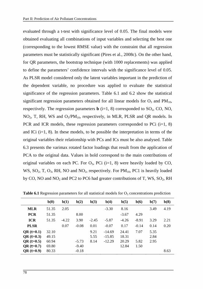
Part II: Prediction of Air Pollutant Concentrations
78
evaluated through a t-test with significance level of 0.05. The final models were
obtained evaluating all combinations of input variables and selecting the best one
(corresponding to the lowest RMSE value) with the constraint that all regression
parameters must be statistically significant (Pires et al., 2008c). On the other hand,
for QR parameters, the bootstrap technique (with 1000 replacements) was applied
to define the parameters’ confidence intervals with the significance level of 0.05.
As PLSR model considered only the latent variables important in the prediction of
the dependent variable, no procedure was applied to evaluate the statistical
significance of the regression parameters. Table 6.1 and 6.2 show the statistical
significant regression parameters obtained for all linear models for O3 and PM10,
respectively. The regression parameters b (i=1, 8) corresponded to SO2, CO, NO,
NO2, T, RH, WS and O3/PM10, respectively, in MLR, PLSR and QR models. In
PCR and ICR models, these regression parameters corresponded to PCi (i=1, 8)
and ICi (i=1, 8). In these models, to be possible the interpretation in terms of the
original variables their relationship with PCs and ICs must be also analysed. Table
6.3 presents the varimax rotated factor loadings that result from the application of
PCA to the original data. Values in bold correspond to the main contributions of
original variables on each PC. For O3, PCi (i=1, 8) were heavily loaded by CO,
WS, SO2, T, O3, RH, NO and NO2, respectively. For PM10, PC1 is heavily loaded
by CO, NO and NO2 and PC2 to PC6 had greater contributions of T, WS, SO2, RH
Table 6.1 Regression parameters for all statistical models for O3 concentrations prediction
b(0) b(1) b(2) b(3) b(4) b(5) b(6) b(7) b(8)
MLR 51.35 2.05 -3.30 8.16 3.49 4.19
PCR 51.35 8.00 -3.67 4.29
ICR 51.35 -4.22 3.90 -2.45 -5.87 -4.26 -8.91 3.29 2.21
PLSR 0.07 -0.08 0.01 -0.07 0.17 -0.14 0.14 0.20
QR (ττττ=0.1) 32.10 9.21 -14.69 24.41 7.07 5.35 QR (ττττ=0.3) 49.15 5.55 -15.85 18.31 2.84 QR (ττττ=0.5) 60.94 -5.73 8.14 -12.29 20.29 5.82 2.95 QR (ττττ=0.7) 69.80 -9.40 12.84 1.50 QR (ττττ=0.9) 80.33 -0.18 8.63
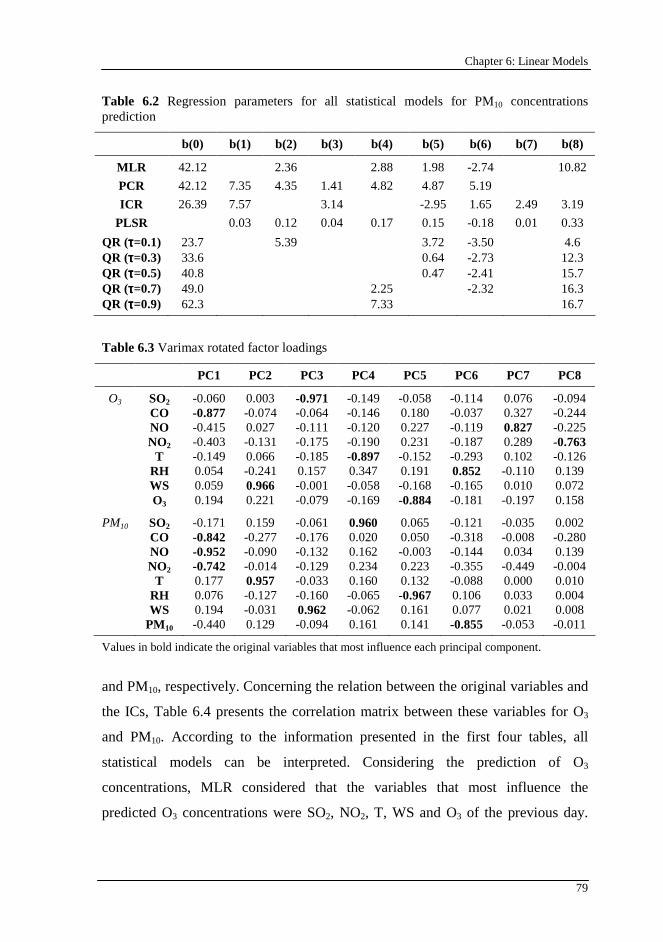
Chapter 6: Linear Models
79
Table 6.2 Regression parameters for all statistical models for PM10 concentrations prediction
b(0) b(1) b(2) b(3) b(4) b(5) b(6) b(7) b(8)
MLR 42.12 2.36 2.88 1.98 -2.74 10.82
PCR 42.12 7.35 4.35 1.41 4.82 4.87 5.19
ICR 26.39 7.57 3.14 -2.95 1.65 2.49 3.19
PLSR 0.03 0.12 0.04 0.17 0.15 -0.18 0.01 0.33
QR (ττττ=0.1) 23.7 5.39 3.72 -3.50 4.6 QR (ττττ=0.3) 33.6 0.64 -2.73 12.3 QR (ττττ=0.5) 40.8 0.47 -2.41 15.7 QR (ττττ=0.7) 49.0 2.25 -2.32 16.3 QR (ττττ=0.9) 62.3 7.33 16.7
Table 6.3 Varimax rotated factor loadings
PC1 PC2 PC3 PC4 PC5 PC6 PC7 PC8
O3 SO2 -0.060 0.003 -0.971 -0.149 -0.058 -0.114 0.076 -0.094 CO -0.877 -0.074 -0.064 -0.146 0.180 -0.037 0.327 -0.244 NO -0.415 0.027 -0.111 -0.120 0.227 -0.119 0.827 -0.225 NO2 -0.403 -0.131 -0.175 -0.190 0.231 -0.187 0.289 -0.763 T -0.149 0.066 -0.185 -0.897 -0.152 -0.293 0.102 -0.126 RH 0.054 -0.241 0.157 0.347 0.191 0.852 -0.110 0.139 WS 0.059 0.966 -0.001 -0.058 -0.168 -0.165 0.010 0.072 O3 0.194 0.221 -0.079 -0.169 -0.884 -0.181 -0.197 0.158
PM10 SO2 -0.171 0.159 -0.061 0.960 0.065 -0.121 -0.035 0.002 CO -0.842 -0.277 -0.176 0.020 0.050 -0.318 -0.008 -0.280 NO -0.952 -0.090 -0.132 0.162 -0.003 -0.144 0.034 0.139 NO2 -0.742 -0.014 -0.129 0.234 0.223 -0.355 -0.449 -0.004 T 0.177 0.957 -0.033 0.160 0.132 -0.088 0.000 0.010 RH 0.076 -0.127 -0.160 -0.065 -0.967 0.106 0.033 0.004 WS 0.194 -0.031 0.962 -0.062 0.161 0.077 0.021 0.008 PM10 -0.440 0.129 -0.094 0.161 0.141 -0.855 -0.053 -0.011
Values in bold indicate the original variables that most influence each principal component.
and PM10, respectively. Concerning the relation between the original variables and
the ICs, Table 6.4 presents the correlation matrix between these variables for O3
and PM10. According to the information presented in the first four tables, all
statistical models can be interpreted. Considering the prediction of O3
concentrations, MLR considered that the variables that most influence the
predicted O3 concentrations were SO2, NO2, T, WS and O3 of the previous day.
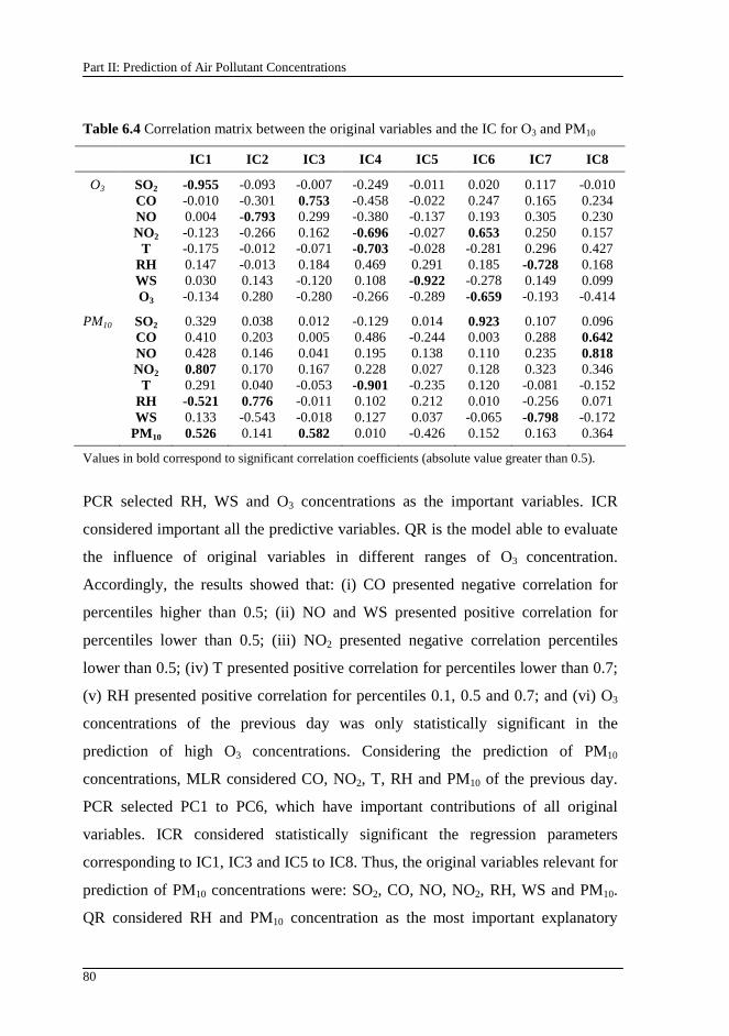
Part II: Prediction of Air Pollutant Concentrations
80
Table 6.4 Correlation matrix between the original variables and the IC for O3 and PM10
IC1 IC2 IC3 IC4 IC5 IC6 IC7 IC8
O3 SO2 -0.955 -0.093 -0.007 -0.249 -0.011 0.020 0.117 -0.010 CO -0.010 -0.301 0.753 -0.458 -0.022 0.247 0.165 0.234 NO 0.004 -0.793 0.299 -0.380 -0.137 0.193 0.305 0.230 NO2 -0.123 -0.266 0.162 -0.696 -0.027 0.653 0.250 0.157 T -0.175 -0.012 -0.071 -0.703 -0.028 -0.281 0.296 0.427 RH 0.147 -0.013 0.184 0.469 0.291 0.185 -0.728 0.168 WS 0.030 0.143 -0.120 0.108 -0.922 -0.278 0.149 0.099 O3 -0.134 0.280 -0.280 -0.266 -0.289 -0.659 -0.193 -0.414
PM10 SO2 0.329 0.038 0.012 -0.129 0.014 0.923 0.107 0.096 CO 0.410 0.203 0.005 0.486 -0.244 0.003 0.288 0.642 NO 0.428 0.146 0.041 0.195 0.138 0.110 0.235 0.818 NO2 0.807 0.170 0.167 0.228 0.027 0.128 0.323 0.346 T 0.291 0.040 -0.053 -0.901 -0.235 0.120 -0.081 -0.152 RH -0.521 0.776 -0.011 0.102 0.212 0.010 -0.256 0.071 WS 0.133 -0.543 -0.018 0.127 0.037 -0.065 -0.798 -0.172 PM10 0.526 0.141 0.582 0.010 -0.426 0.152 0.163 0.364
Values in bold correspond to significant correlation coefficients (absolute value greater than 0.5).
PCR selected RH, WS and O3 concentrations as the important variables. ICR
considered important all the predictive variables. QR is the model able to evaluate
the influence of original variables in different ranges of O3 concentration.
Accordingly, the results showed that: (i) CO presented negative correlation for
percentiles higher than 0.5; (ii) NO and WS presented positive correlation for
percentiles lower than 0.5; (iii) NO2 presented negative correlation percentiles
lower than 0.5; (iv) T presented positive correlation for percentiles lower than 0.7;
(v) RH presented positive correlation for percentiles 0.1, 0.5 and 0.7; and (vi) O3
concentrations of the previous day was only statistically significant in the
prediction of high O3 concentrations. Considering the prediction of PM10
concentrations, MLR considered CO, NO2, T, RH and PM10 of the previous day.
PCR selected PC1 to PC6, which have important contributions of all original
variables. ICR considered statistically significant the regression parameters
corresponding to IC1, IC3 and IC5 to IC8. Thus, the original variables relevant for
prediction of PM10 concentrations were: SO2, CO, NO, NO2, RH, WS and PM10.
QR considered RH and PM10 concentration as the most important explanatory
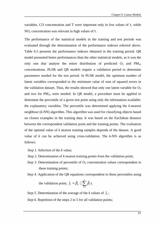
Chapter 6: Linear Models
81
variables. CO concentration and T were important only in low values of τ, while
NO2 concentration was relevant in high values of τ.
The performance of the statistical models in the training and test periods was
evaluated through the determination of the performance indexes referred above.
Table 6.5 presents the performance indexes obtained in the training period. QR
model presented better performances than the other statistical models, as it was the
only one that analyse the entire distribution of predicted O3 and PM10
concentrations. PLSR and QR models require a validation period to determine
parameters needed for the test period. In PLSR model, the optimum number of
latent variables corresponded to the minimum value of sum of squared errors in
the validation dataset. Thus, the results showed that only one latent variable for O3
and two for PM10 were needed. In QR model, a procedure must be applied to
determine the percentile of a given test point using only the information available:
the explanatory variables. The percentile was determined applying the k-nearest
neighbour (k-NN) algorithm. This algorithm was used for classifying objects based
on closest examples in the training data. It was based on the Euclidean distance
between the correspondent validation point and the training points. The evaluation
of the optimal value of k nearest training samples depends of the dataset. A good
value of k can be achieved using cross-validation. The k-NN algorithm is as
follows:
Step 1. Selection of the k value;
Step 2. Determination of k nearest training points from the validation point;
Step 3. Determination of percentile of O3 concentration values correspondent to
these training points;
Step 4. Application of the QR equations correspondent to these percentiles using
the validation point; i
k
1ii0i xy ∑
=
+= ββ ˆˆˆ
Step 5. Determination of the average of the k values of iy ;
Step 6. Repetition of the steps 2 to 5 for all validation points;
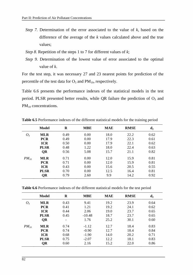
Part II: Prediction of Air Pollutant Concentrations
82
Step 7. Determination of the error associated to the value of k, based on the
difference of the average of the k values calculated above and the true
values;
Step 8. Repetition of the steps 1 to 7 for different values of k;
Step 9. Determination of the lowest value of error associated to the optimal
value of k.
For the test step, it was necessary 27 and 23 nearest points for prediction of the
percentile of the test data for O3 and PM10, respectively.
Table 6.6 presents the performance indexes of the statistical models in the test
period. PLSR presented better results, while QR failure the prediction of O3 and
PM10 concentrations.
Table 6.5 Performance indexes of the different statistical models for the training period
Model R MBE MAE RMSE d 2
O3 MLR 0.49 0.00 18.0 22.2 0.62 PCR 0.49 0.00 17.9 22.3 0.61 ICR 0.50 0.00 17.9 22.1 0.62 PLSR 0.48 1.22 18.0 22.4 0.63 QR 0.56 5.08 15.7 21.1 0.82
PM10 MLR 0.71 0.00 12.0 15.9 0.81 PCR 0.71 0.00 12.0 15.9 0.81 ICR 0.43 0.00 15.6 20.5 0.55 PLSR 0.70 0.00 12.5 16.4 0.81 QR 0.79 2.60 9.9 14.2 0.92
Table 6.6 Performance indexes of the different statistical models for the test period
Model R MBE MAE RMSE d 2
O3 MLR 0.43 9.41 19.2 23.9 0.64 PCR 0.41 1.21 19.2 24.1 0.62 ICR 0.44 2.06 19.0 23.7 0.65 PLSR 0.45 -10.48 18.7 23.7 0.65 QR - 1.76 25.2 30.1 0.60
PM10 MLR 0.74 -1.12 12.7 18.4 0.83 PCR 0.74 -0.90 12.7 18.4 0.84 ICR 0.68 -1.90 14.0 20.2 0.71 PLSR 0.75 -2.07 12.2 18.1 0.83 QR 0.60 2.16 15.2 22.0 0.86
Chapter 6: Linear Models
83
6.10. Conclusions
Five linear models were applied to predict the next day hourly average O3
concentrations and the daily average PM10 concentrations, using as predictors
environmental and meteorological data. At same time, the importance of each
predictor in the air pollutants formation was analysed based on the statistically
significant regression parameters for each model. QR model presented better
performance in the training period, because it tries to model the entire distribution
of the output value. However, it presented worst predictions in the test period. This
means that a new procedure should be found better than k-NN algorithm to
estimate the percentiles of the output variable in the test dataset with more
precision. Concluding, the PLSR presented better predictive performance than the
other linear models.

85
Chapter 7
7. Stepwise artificial neural networks
This chapter shows the comparison of two systematic methodologies to build artificial neural network models for predicting the hourly average of O3 concentrations and the daily average of PM10 concentrations of the next day. They consist in: (i) adding hidden neurons one by one and (ii) adding input-to-hidden layer synapses one by one. Different types of input variables were tested: original variables, principal components and independent components. In addition, several activation functions were used for the hidden nodes: sigmoid, hyperbolic tangent and sine functions.
The contents of this chapter were adapted from: Pires, J.C.M., Martins, F.G., Alvim-Ferraz, M.C.M., Pereira, M.C., 2009. Stepwise artificial neural networks for predicting tropospheric ozone and PM10 concentrations. Submitted for publication.
7.1. Introduction
The artificial neural networks (ANNs) are one of the most used nonlinear models
for the prediction of O3 (Heo and Kim, 2004; Sousa et al., 2006, 2007) and PM10
concentrations (Grivas and Chaloulakou, 2006; Perez and Reyes, 2002, 2006).
ANN are adaptive statistical models inspired in the biological neural processing
system (Tang et al., 2001; Tawadrous and Katsabanis, 2006). The artificial
neurons of the networks are modelled attempting to mimic the performances of
neural cells in the brain. The first mathematical approach of this method was done
with the introduction of simplified neurons by McCulloch and Pitts in 1943
(Montague and Quartz, 1999; Tang et al., 2001; Tawadrous and Katsabanis, 2006).
After a period of few applicability of these models, ANN only acquired great
Part II: Prediction of Air Pollutant Concentrations
86
importance in the field of statistical models with: (i) the introduction of the
backpropagation algorithm in the learning step, and (ii) the development of new
hardware which increased the processing capacities (Tawadrous and Katsabanis,
2006), really important for their application.
ANN can perform several functions such as classification, regression, association
and mapping tasks (Corne, 1998; Perez and Reyes, 2002, 2006; Sousa et al., 2006,
2007). They are applied to a wide variety of problems including adaptive control,
optimization, medical diagnosis, decision making, as well as in information, signal
and speech processing (Gupta and Achenie, 2007; Nagy, 2007; Uncini, 2003).
ANN models are characterized by: (i) a set of processing neurons (also designated
by nodes); (ii) a pattern of connectivity among neurons; (iii) an activation function
for each neuron; and (iv) a learning rule. The processing neurons are distributed in
layers (Qingbin et al., 1996): (i) input layer (first layer); (ii) output layer (last
layer); and (iii) hidden layers (layers between the input and the output layers). The
neurons in different layers are linked by synapses (each one storing a weight
value) and the way which these linkages are done defines the structure of the
network. There are two main network topologies (Chiang et al., 2004; Pacella and
Semeraro, 2007): (i) feedforward networks; and (ii) recurrent networks. In the first
one, the information flows only feedforward, from input to output neurons. These
networks do not present connections starting in outputs of neurons and ending in
inputs of neurons in the same layer or previous layers (feedback connections).
Recurrent networks derived from feedforward networks, presenting the two types
of connections, the feedforward and the feedback (Arsie et al., 2006; Hu et al.,
2007; Yang and Ni, 2005).
The neuron processes the information received by the inputs and calculates an
output. An activation function is generally used in which the common functions
are: (i) the pure linear; (ii) the sigmoid; and (iii) the hyperbolic tangent
(Hernández-Caraballo and Marcó-Parra, 2003). However, many others can be also
applied. Besides the inputs, a bias is also used in each processing neuron. Biases
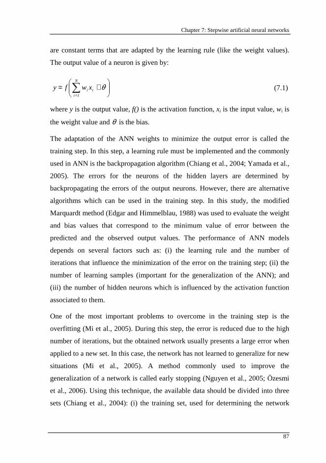
Chapter 7: Stepwise artificial neural networks
87
are constant terms that are adapted by the learning rule (like the weight values).
The output value of a neuron is given by:
+= ∑
=
N
1iii xwfy θ (7.1)
where y is the output value, f() is the activation function, xi is the input value, wi is
the weight value and θ is the bias.
The adaptation of the ANN weights to minimize the output error is called the
training step. In this step, a learning rule must be implemented and the commonly
used in ANN is the backpropagation algorithm (Chiang et al., 2004; Yamada et al.,
2005). The errors for the neurons of the hidden layers are determined by
backpropagating the errors of the output neurons. However, there are alternative
algorithms which can be used in the training step. In this study, the modified
Marquardt method (Edgar and Himmelblau, 1988) was used to evaluate the weight
and bias values that correspond to the minimum value of error between the
predicted and the observed output values. The performance of ANN models
depends on several factors such as: (i) the learning rule and the number of
iterations that influence the minimization of the error on the training step; (ii) the
number of learning samples (important for the generalization of the ANN); and
(iii) the number of hidden neurons which is influenced by the activation function
associated to them.
One of the most important problems to overcome in the training step is the
overfitting (Mi et al., 2005). During this step, the error is reduced due to the high
number of iterations, but the obtained network usually presents a large error when
applied to a new set. In this case, the network has not learned to generalize for new
situations (Mi et al., 2005). A method commonly used to improve the
generalization of a network is called early stopping (Nguyen et al., 2005; Özesmi
et al., 2006). Using this technique, the available data should be divided into three
sets (Chiang et al., 2004): (i) the training set, used for determining the network
Part II: Prediction of Air Pollutant Concentrations
88
weights and biases; (ii) the validation set, used to evaluate the performance of
ANN during the training step (the increase of validation error stops the training
process); and (iii) the test set, used to evaluate the ANN performance.
As it happens in the linear models, ANN is also influenced by the collinearity of
the input variables. In this study, two different methods were used to remove the
correlation between the original variables (OVs): (i) principal component analysis
(PCA) and (ii) independent component analysis (ICA). These statistical methods
were described in Chapter 6.
An additional problem to build ANN models is to achieve the adequate network
complexity which includes the determination of the significance of each weight
value in the network, as it is done for coefficients of linear regressions (Pires et al.,
2008c), and the definition of the number of hidden neurons. In general there are
two fundamentals to build ANN models (Ghiassi and Saidane, 2005; Medeiros et
al., 2006; Rivals and Personnaz, 2003). The first one is called growing approach
that begins with a simple network and iteratively adds hidden nodes and hidden
layers. The second one is called pruning approach that begins with a large network
with low training error and prunes the weights and biases whose removal increase
the training error at least. After the removal, the network must be retrained to
enhance its performance. Besides the weights, this method can prune also the
neurons. The pruning of all input or output weights of a neuron is equivalent to
prune the neuron itself.
7.2. Stepwise artificial neural networks
Stepwise artificial neural networks (SWANNs) are systematic methodologies to
build ANN models in which it is not needed to define the structure in advance.
The size of the ANN structures is determined during the training step. The two
SWANNs here reported are based on feedforward neural networks with a single
hidden layer. The first SWANN, designated by SWANN1, corresponds to the
addition of hidden neurons one by one. The second SWANN (SWANN2) is based
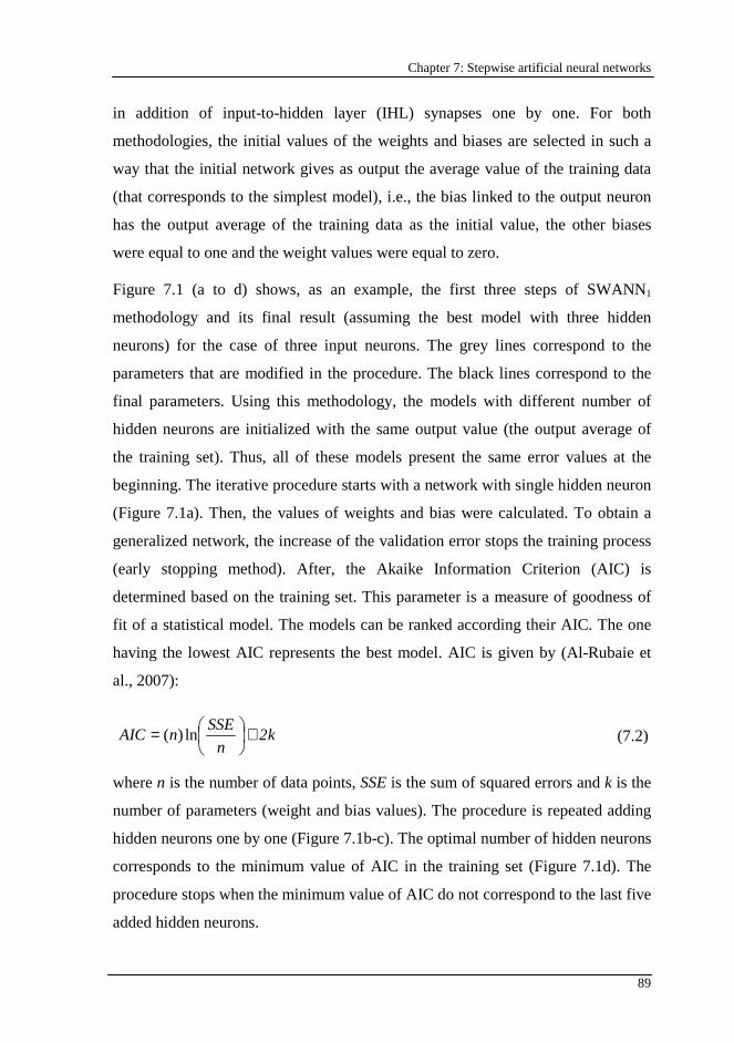
Chapter 7: Stepwise artificial neural networks
89
in addition of input-to-hidden layer (IHL) synapses one by one. For both
methodologies, the initial values of the weights and biases are selected in such a
way that the initial network gives as output the average value of the training data
(that corresponds to the simplest model), i.e., the bias linked to the output neuron
has the output average of the training data as the initial value, the other biases
were equal to one and the weight values were equal to zero.
Figure 7.1 (a to d) shows, as an example, the first three steps of SWANN1
methodology and its final result (assuming the best model with three hidden
neurons) for the case of three input neurons. The grey lines correspond to the
parameters that are modified in the procedure. The black lines correspond to the
final parameters. Using this methodology, the models with different number of
hidden neurons are initialized with the same output value (the output average of
the training set). Thus, all of these models present the same error values at the
beginning. The iterative procedure starts with a network with single hidden neuron
(Figure 7.1a). Then, the values of weights and bias were calculated. To obtain a
generalized network, the increase of the validation error stops the training process
(early stopping method). After, the Akaike Information Criterion (AIC) is
determined based on the training set. This parameter is a measure of goodness of
fit of a statistical model. The models can be ranked according their AIC. The one
having the lowest AIC represents the best model. AIC is given by (Al-Rubaie et
al., 2007):
k2n
SSEnAIC +
= ln)( (7.2)
where n is the number of data points, SSE is the sum of squared errors and k is the
number of parameters (weight and bias values). The procedure is repeated adding
hidden neurons one by one (Figure 7.1b-c). The optimal number of hidden neurons
corresponds to the minimum value of AIC in the training set (Figure 7.1d). The
procedure stops when the minimum value of AIC do not correspond to the last five
added hidden neurons.
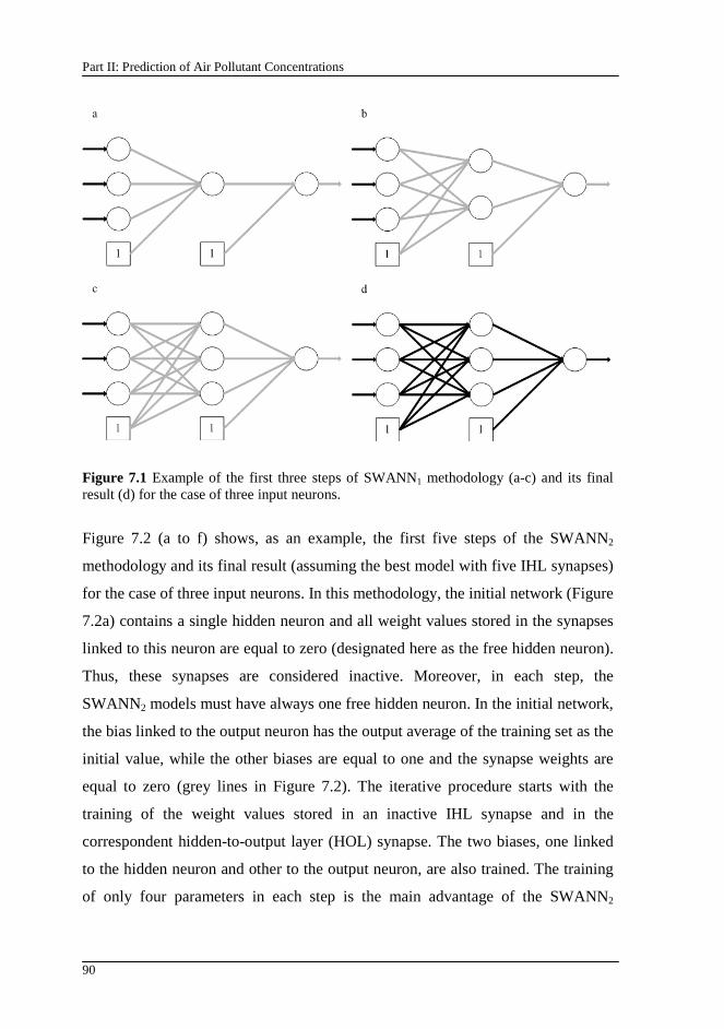
Part II: Prediction of Air Pollutant Concentrations
90
Figure 7.1 Example of the first three steps of SWANN1 methodology (a-c) and its final result (d) for the case of three input neurons.
Figure 7.2 (a to f) shows, as an example, the first five steps of the SWANN2
methodology and its final result (assuming the best model with five IHL synapses)
for the case of three input neurons. In this methodology, the initial network (Figure
7.2a) contains a single hidden neuron and all weight values stored in the synapses
linked to this neuron are equal to zero (designated here as the free hidden neuron).
Thus, these synapses are considered inactive. Moreover, in each step, the
SWANN2 models must have always one free hidden neuron. In the initial network,
the bias linked to the output neuron has the output average of the training set as the
initial value, while the other biases are equal to one and the synapse weights are
equal to zero (grey lines in Figure 7.2). The iterative procedure starts with the
training of the weight values stored in an inactive IHL synapse and in the
correspondent hidden-to-output layer (HOL) synapse. The two biases, one linked
to the hidden neuron and other to the output neuron, are also trained. The training
of only four parameters in each step is the main advantage of the SWANN2
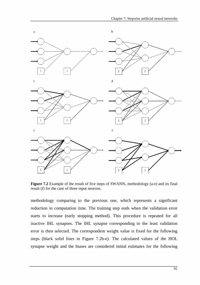
Chapter 7: Stepwise artificial neural networks
91
Figure 7.2 Example of the result of five steps of SWANN2 methodology (a-e) and its final result (f) for the case of three input neurons.
methodology comparing to the previous one, which represents a significant
reduction in computation time. The training step ends when the validation error
starts to increase (early stopping method). This procedure is repeated for all
inactive IHL synapses. The IHL synapse corresponding to the least validation
error is then selected. The correspondent weight value is fixed for the following
steps (black solid lines in Figure 7.2b-e). The calculated values of the HOL
synapse weight and the biases are considered initial estimates for the following
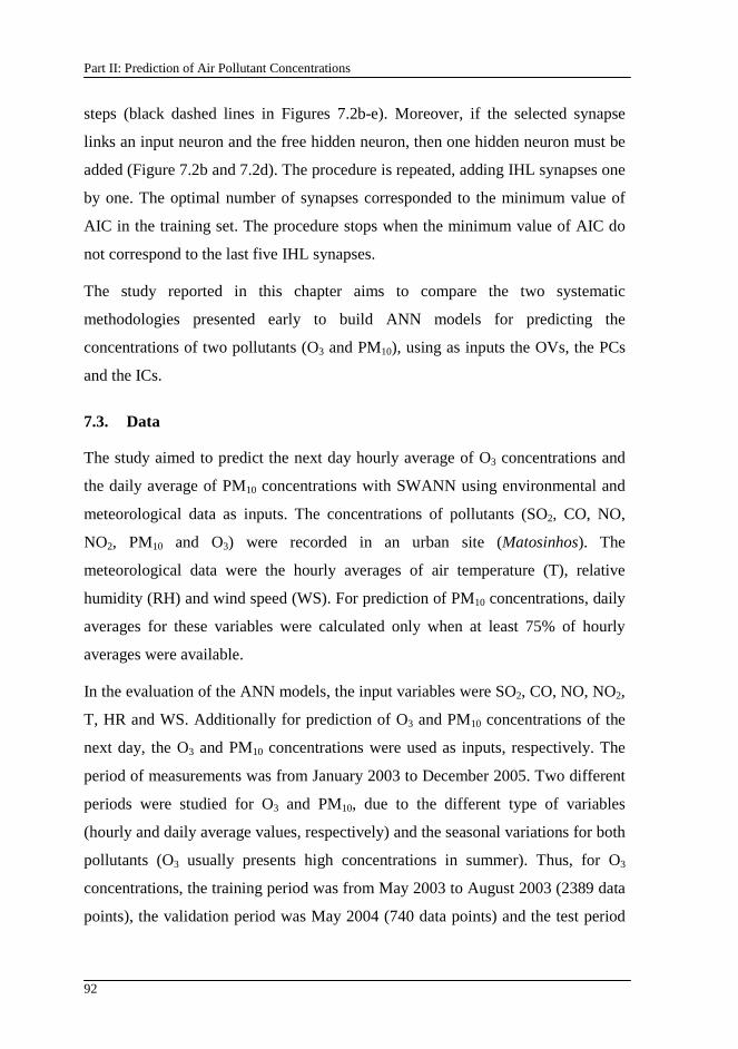
Part II: Prediction of Air Pollutant Concentrations
92
steps (black dashed lines in Figures 7.2b-e). Moreover, if the selected synapse
links an input neuron and the free hidden neuron, then one hidden neuron must be
added (Figure 7.2b and 7.2d). The procedure is repeated, adding IHL synapses one
by one. The optimal number of synapses corresponded to the minimum value of
AIC in the training set. The procedure stops when the minimum value of AIC do
not correspond to the last five IHL synapses.
The study reported in this chapter aims to compare the two systematic
methodologies presented early to build ANN models for predicting the
concentrations of two pollutants (O3 and PM10), using as inputs the OVs, the PCs
and the ICs.
7.3. Data
The study aimed to predict the next day hourly average of O3 concentrations and
the daily average of PM10 concentrations with SWANN using environmental and
meteorological data as inputs. The concentrations of pollutants (SO2, CO, NO,
NO2, PM10 and O3) were recorded in an urban site (Matosinhos). The
meteorological data were the hourly averages of air temperature (T), relative
humidity (RH) and wind speed (WS). For prediction of PM10 concentrations, daily
averages for these variables were calculated only when at least 75% of hourly
averages were available.
In the evaluation of the ANN models, the input variables were SO2, CO, NO, NO2,
T, HR and WS. Additionally for prediction of O3 and PM10 concentrations of the
next day, the O3 and PM10 concentrations were used as inputs, respectively. The
period of measurements was from January 2003 to December 2005. Two different
periods were studied for O3 and PM10, due to the different type of variables
(hourly and daily average values, respectively) and the seasonal variations for both
pollutants (O3 usually presents high concentrations in summer). Thus, for O3
concentrations, the training period was from May 2003 to August 2003 (2389 data
points), the validation period was May 2004 (740 data points) and the test period
Chapter 7: Stepwise artificial neural networks
93
was June 2004 (periods when high O3 concentrations are frequently measured; 715
data points). For PM10 concentrations, the forth quarter of 2004 was considered as
validation period (88 data points), the corresponding period of 2005 (76 data
points) as test period and the remained data from 2003 to 2005 as training period
(826 data points). The explanatory variables were Z standardized to have zero
mean and unit standard deviation.
7.4. Results and discussion
SWANN1 and SWANN2 were applied to predict O3 and PM10 concentrations,
using OVs, PCs and ICs as input variables. The PCs were determined using a
subroutine developed in Microsoft Visual Basic Applications for Microsoft Excel
created by the author of this thesis. The ICs were obtained using the FastICA
package (available in http://www.cis.hut.fi/projects/ica/fastica/) for Matlab. The
author of this thesis also developed the code in Matlab to achieve the SWANN1
and SWANN2 models. Different activation functions were also used: (i) sigmoid
function (sig); (ii) hyperbolic tangent function (tgh); and (iii) sine function (sin).
Figure 7.3 shows, as an example, the variation of AIC value in the training set
with the increase of number of IHL synapses in SWANN2 models, using OVs as
inputs and the activation function sine. In this case, the minimum value of AIC
14800
14900
15000
15100
15200
15300
0 20 40 60 80 100
IHL Synapses
AIC
val
ue
Figure 7.3 Variation of AIC value in the training set with the increase of the number of IHL synapses in SWANN2 models using OVs as inputs and the activation function sine.
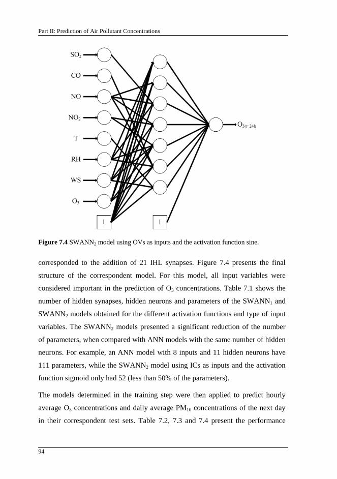
Part II: Prediction of Air Pollutant Concentrations
94
Figure 7.4 SWANN2 model using OVs as inputs and the activation function sine.
corresponded to the addition of 21 IHL synapses. Figure 7.4 presents the final
structure of the correspondent model. For this model, all input variables were
considered important in the prediction of O3 concentrations. Table 7.1 shows the
number of hidden synapses, hidden neurons and parameters of the SWANN1 and
SWANN2 models obtained for the different activation functions and type of input
variables. The SWANN2 models presented a significant reduction of the number
of parameters, when compared with ANN models with the same number of hidden
neurons. For example, an ANN model with 8 inputs and 11 hidden neurons have
111 parameters, while the SWANN2 model using ICs as inputs and the activation
function sigmoid only had 52 (less than 50% of the parameters).
The models determined in the training step were then applied to predict hourly
average O3 concentrations and daily average PM10 concentrations of the next day
in their correspondent test sets. Table 7.2, 7.3 and 7.4 present the performance
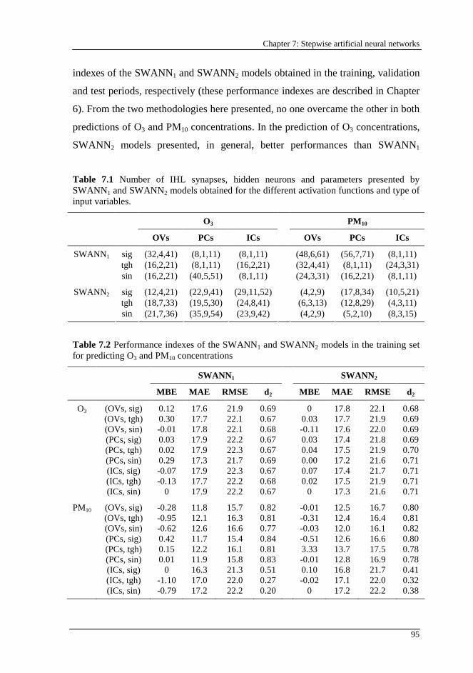
Chapter 7: Stepwise artificial neural networks
95
indexes of the SWANN1 and SWANN2 models obtained in the training, validation
and test periods, respectively (these performance indexes are described in Chapter
6). From the two methodologies here presented, no one overcame the other in both
predictions of O3 and PM10 concentrations. In the prediction of O3 concentrations,
SWANN2 models presented, in general, better performances than SWANN1
Table 7.1 Number of IHL synapses, hidden neurons and parameters presented by SWANN1 and SWANN2 models obtained for the different activation functions and type of input variables.
O3 PM10
OVs PCs ICs OVs PCs ICs
sig (32,4,41) (8,1,11) (8,1,11) (48,6,61) (56,7,71) (8,1,11) tgh (16,2,21) (8,1,11) (16,2,21) (32,4,41) (8,1,11) (24,3,31)
SWANN1
sin (16,2,21) (40,5,51) (8,1,11) (24,3,31) (16,2,21) (8,1,11)
sig (12,4,21) (22,9,41) (29,11,52) (4,2,9) (17,8,34) (10,5,21) tgh (18,7,33) (19,5,30) (24,8,41) (6,3,13) (12,8,29) (4,3,11)
SWANN2
sin (21,7,36) (35,9,54) (23,9,42) (4,2,9) (5,2,10) (8,3,15)
Table 7.2 Performance indexes of the SWANN1 and SWANN2 models in the training set for predicting O3 and PM10 concentrations
SWANN1 SWANN2
MBE MAE RMSE d 2 MBE MAE RMSE d 2
O3 (OVs, sig) 0.12 17.6 21.9 0.69 0 17.8 22.1 0.68 (OVs, tgh) 0.30 17.7 22.1 0.67 0.03 17.7 21.9 0.69 (OVs, sin) -0.01 17.8 22.1 0.68 -0.11 17.6 22.0 0.69 (PCs, sig) 0.03 17.9 22.2 0.67 0.03 17.4 21.8 0.69 (PCs, tgh) 0.02 17.9 22.3 0.67 0.04 17.5 21.9 0.70 (PCs, sin) 0.29 17.3 21.7 0.69 0.00 17.2 21.6 0.71 (ICs, sig) -0.07 17.9 22.3 0.67 0.07 17.4 21.7 0.71 (ICs, tgh) -0.13 17.7 22.2 0.68 0.02 17.5 21.9 0.71 (ICs, sin) 0 17.9 22.2 0.67 0 17.3 21.6 0.71
PM10 (OVs, sig) -0.28 11.8 15.7 0.82 -0.01 12.5 16.7 0.80 (OVs, tgh) -0.95 12.1 16.3 0.81 -0.31 12.4 16.4 0.81 (OVs, sin) -0.62 12.6 16.6 0.77 -0.03 12.0 16.1 0.82 (PCs, sig) 0.42 11.7 15.4 0.84 -0.51 12.6 16.6 0.80 (PCs, tgh) 0.15 12.2 16.1 0.81 3.33 13.7 17.5 0.78 (PCs, sin) 0.01 11.9 15.8 0.83 -0.01 12.8 16.9 0.78 (ICs, sig) 0 16.3 21.3 0.51 0.10 16.8 21.7 0.41 (ICs, tgh) -1.10 17.0 22.0 0.27 -0.02 17.1 22.0 0.32 (ICs, sin) -0.79 17.2 22.2 0.20 0 17.2 22.2 0.38
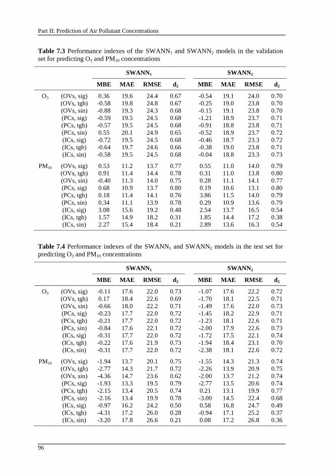
Part II: Prediction of Air Pollutant Concentrations
96
Table 7.3 Performance indexes of the SWANN1 and SWANN2 models in the validation set for predicting O3 and PM10 concentrations
SWANN1 SWANN2
MBE MAE RMSE d 2 MBE MAE RMSE d 2
O3 (OVs, sig) 0.36 19.6 24.4 0.67 -0.54 19.1 24.0 0.70 (OVs, tgh) -0.58 19.8 24.8 0.67 -0.25 19.0 23.8 0.70 (OVs, sin) -0.88 19.3 24.3 0.68 -0.15 19.1 23.8 0.70 (PCs, sig) -0.59 19.5 24.5 0.68 -1.21 18.9 23.7 0.71 (PCs, tgh) -0.57 19.5 24.5 0.68 -0.91 18.8 23.8 0.71 (PCs, sin) 0.55 20.1 24.9 0.65 -0.52 18.9 23.7 0.72 (ICs, sig) -0.72 19.5 24.5 0.68 -0.46 18.7 23.3 0.72 (ICs, tgh) -0.64 19.7 24.6 0.66 -0.38 19.0 23.8 0.71 (ICs, sin) -0.58 19.5 24.5 0.68 -0.04 18.8 23.3 0.73
PM10 (OVs, sig) 0.53 11.2 13.7 0.77 0.55 11.0 14.0 0.79 (OVs, tgh) 0.91 11.4 14.4 0.78 0.31 11.0 13.8 0.80 (OVs, sin) -0.40 11.3 14.0 0.75 0.28 11.1 14.1 0.77 (PCs, sig) 0.68 10.9 13.7 0.80 0.19 10.6 13.1 0.80 (PCs, tgh) 0.18 11.4 14.1 0.76 3.86 11.5 14.0 0.79 (PCs, sin) 0.34 11.1 13.9 0.78 0.29 10.9 13.6 0.79 (ICs, sig) 3.08 15.6 19.2 0.48 2.54 13.7 16.5 0.54 (ICs, tgh) 1.57 14.9 18.2 0.31 1.85 14.4 17.2 0.38 (ICs, sin) 2.27 15.4 18.4 0.21 2.89 13.6 16.3 0.54
Table 7.4 Performance indexes of the SWANN1 and SWANN2 models in the test set for predicting O3 and PM10 concentrations
SWANN1 SWANN2
MBE MAE RMSE d 2 MBE MAE RMSE d 2
O3 (OVs, sig) -0.11 17.6 22.0 0.73 -1.07 17.6 22.2 0.72 (OVs, tgh) 0.17 18.4 22.6 0.69 -1.70 18.1 22.5 0.71 (OVs, sin) -0.66 18.0 22.2 0.71 -1.49 17.6 22.0 0.73 (PCs, sig) -0.23 17.7 22.0 0.72 -1.45 18.2 22.9 0.71 (PCs, tgh) -0.21 17.7 22.0 0.72 -1.23 18.1 22.6 0.71 (PCs, sin) -0.84 17.6 22.1 0.72 -2.00 17.9 22.6 0.73 (ICs, sig) -0.31 17.7 22.0 0.72 -1.72 17.5 22.1 0.74 (ICs, tgh) -0.22 17.6 21.9 0.73 -1.94 18.4 23.1 0.70 (ICs, sin) -0.31 17.7 22.0 0.72 -2.38 18.1 22.6 0.72
PM10 (OVs, sig) -1.94 13.7 20.1 0.75 -1.55 14.3 21.3 0.74 (OVs, tgh) -2.77 14.3 21.7 0.72 -2.26 13.9 20.9 0.75 (OVs, sin) -4.36 14.7 23.6 0.62 -2.00 13.7 21.2 0.74 (PCs, sig) -1.93 13.3 19.5 0.79 -2.77 13.5 20.6 0.74 (PCs, tgh) -2.15 13.4 20.5 0.74 0.21 13.1 19.9 0.77 (PCs, sin) -2.16 13.4 19.9 0.78 -3.00 14.5 22.4 0.68 (ICs, sig) -0.97 16.2 24.2 0.50 0.58 16.8 24.7 0.49 (ICs, tgh) -4.31 17.2 26.0 0.28 -0.94 17.1 25.2 0.37 (ICs, sin) -3.20 17.8 26.6 0.21 0.08 17.2 26.8 0.36
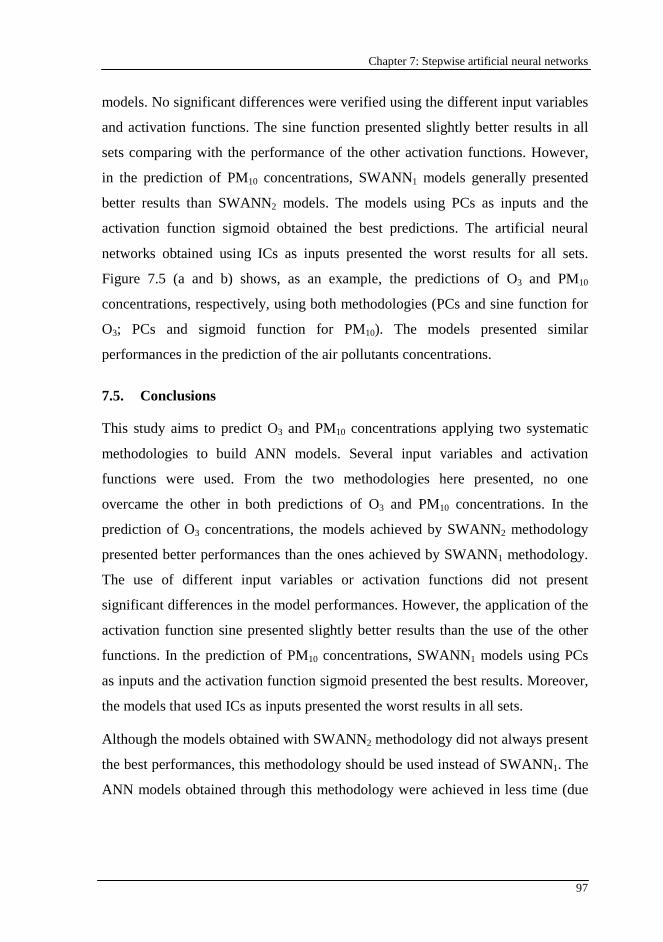
Chapter 7: Stepwise artificial neural networks
97
models. No significant differences were verified using the different input variables
and activation functions. The sine function presented slightly better results in all
sets comparing with the performance of the other activation functions. However,
in the prediction of PM10 concentrations, SWANN1 models generally presented
better results than SWANN2 models. The models using PCs as inputs and the
activation function sigmoid obtained the best predictions. The artificial neural
networks obtained using ICs as inputs presented the worst results for all sets.
Figure 7.5 (a and b) shows, as an example, the predictions of O3 and PM10
concentrations, respectively, using both methodologies (PCs and sine function for
O3; PCs and sigmoid function for PM10). The models presented similar
performances in the prediction of the air pollutants concentrations.
7.5. Conclusions
This study aims to predict O3 and PM10 concentrations applying two systematic
methodologies to build ANN models. Several input variables and activation
functions were used. From the two methodologies here presented, no one
overcame the other in both predictions of O3 and PM10 concentrations. In the
prediction of O3 concentrations, the models achieved by SWANN2 methodology
presented better performances than the ones achieved by SWANN1 methodology.
The use of different input variables or activation functions did not present
significant differences in the model performances. However, the application of the
activation function sine presented slightly better results than the use of the other
functions. In the prediction of PM10 concentrations, SWANN1 models using PCs
as inputs and the activation function sigmoid presented the best results. Moreover,
the models that used ICs as inputs presented the worst results in all sets.
Although the models obtained with SWANN2 methodology did not always present
the best performances, this methodology should be used instead of SWANN1. The
ANN models obtained through this methodology were achieved in less time (due
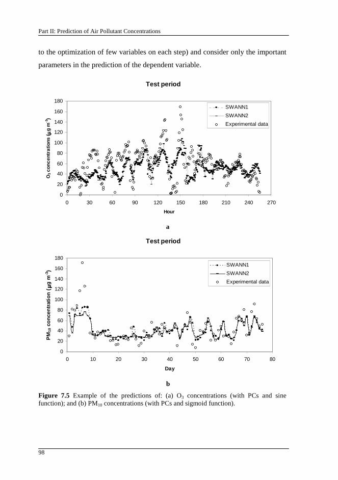
Part II: Prediction of Air Pollutant Concentrations
98
to the optimization of few variables on each step) and consider only the important
parameters in the prediction of the dependent variable.
Test period
0
20
40
60
80
100
120
140
160
180
0 30 60 90 120 150 180 210 240 270
Hour
O3 c
once
ntra
tions
( µµ µµg
m-3
)
SWANN1
SWANN2
Experimental data
a
Test period
0
20
40
60
80
100
120
140
160
180
0 10 20 30 40 50 60 70 80
Day
PM
10 c
on
cen
trat
ion
(µµ µµg
m-3
)
SWANN1
SWANN2
Experimental data
b
Figure 7.5 Example of the predictions of: (a) O3 concentrations (with PCs and sine function); and (b) PM10 concentrations (with PCs and sigmoid function).
99
Chapter 8
8. Threshold regression models
This chapter proposes a new technique based on genetic algorithms to define threshold regression models (TR-GA). The threshold regression assumes that the behaviour of the dependent variable changes when it enters in a different regime. The change from one regime to another depends of a specific value (threshold value) of an explanatory variable (threshold variable). In this study, the threshold regression models were composed by two linear equations. The application of genetic algorithms allows evaluating, at the same time: (i) the threshold variable; (ii) the threshold value; and (iii) the statistically significant regression parameters in each regime. The aim of this study was to evaluate the performance of TR-GA models in the prediction of next day hourly average O3 concentrations.
The contents of this chapter were adapted from: Pires, J.C.M., Martins, F.G., Alvim-Ferraz, M.C.M., Pereira, M.C., 2008. Genetic Algorithm Based Technique for Defining Threshold Regression Models, Proceedings of iEMSs 2008: International Congress on Environmental Modelling and Software, 303-311.
8.1. Introduction
The threshold regression assumes that the behaviour of the dependent variable
changes when it enters in a different regime (Terui and Dijk, 2002). The change
from one regime to another depends of a specific value (threshold value) of an
explanatory variable (threshold variable) (Fouquau et al., 2007). The dependent
variable is given by:
Part II: Prediction of Air Pollutant Concentrations
100
>++
≤++=
∑
∑
=
=k
1id2ii0
k
1id1ii0
i
rxifx
rxifxy
,ˆˆ
,ˆˆ
εββ
εαα (8.1)
where xi (i=1,…,k) are the explanatory variables, iα and iβ (i=0,…,k) are the
regression parameters, ε1 and ε2 are the errors associated with the regressions, r is
the threshold value and xd is the threshold variable (one of the explanatory
variables) that determines the division of the original data in two parts (Terui and
Dijk, 2002). Multiple linear regression (MLR) was then applied to each part of the
data and the regression parameters were determined through the minimization of
the sum of squared errors (Pires et al., 2008c). In both regression equations, only
the statistically significant regression parameters should be considered. The
evaluation of statistical significance of the regression parameters was described in
Chapter 6.
Genetic algorithms (GAs) were applied to the threshold regression model (TR-GA
model), aiming to optimize the values of r (threshold value) and d (index of
threshold variable) with the constraint of all regression parameters must be
statistically significant. The main objective of this study was to evaluate the
performance of TR-GA models in the prediction of the next day hourly average
ozone (O3|t+24h) concentrations.
8.2. Genetic algorithms and TR-GA procedure
GA is a search methodology based on the mechanics of natural selection and
population genetics (Goldberg, 1989; Holland, 1975). This method starts with a set
of individuals (the population) chosen randomly. These individuals (also called
chromosomes) have genes that represent a solution of a given problem. GA
generates a sequence of populations (the generations) by applying the genetic
operators (selection, crossover and mutation) to the individuals. GA presents the
following advantages: (i) optimization with continuous or discrete variables; (ii)
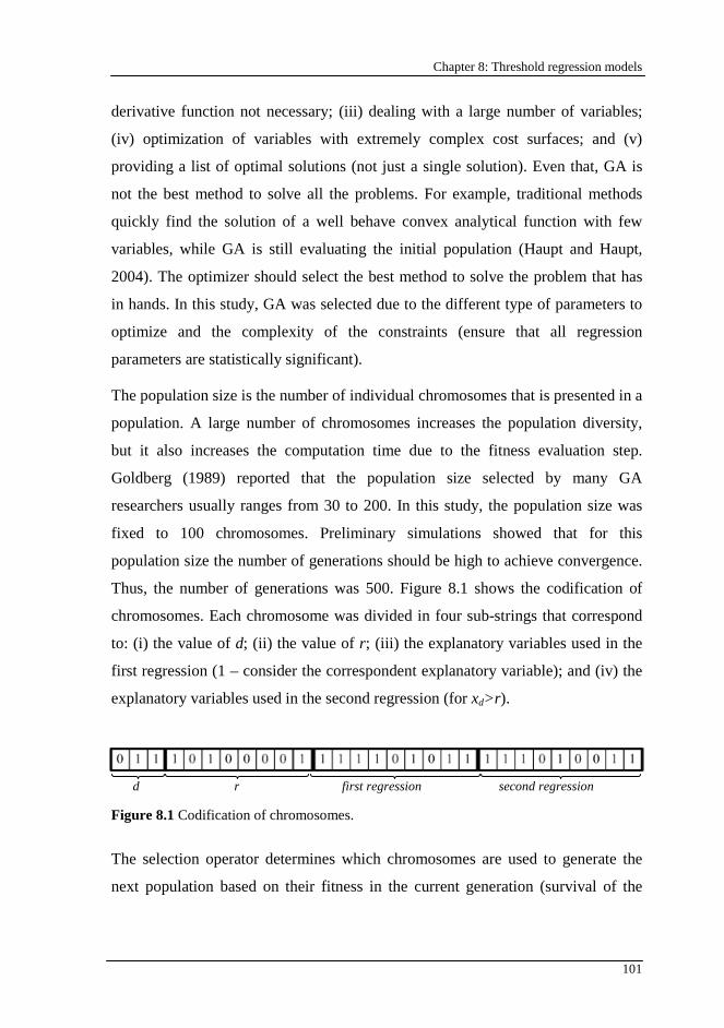
Chapter 8: Threshold regression models
101
derivative function not necessary; (iii) dealing with a large number of variables;
(iv) optimization of variables with extremely complex cost surfaces; and (v)
providing a list of optimal solutions (not just a single solution). Even that, GA is
not the best method to solve all the problems. For example, traditional methods
quickly find the solution of a well behave convex analytical function with few
variables, while GA is still evaluating the initial population (Haupt and Haupt,
2004). The optimizer should select the best method to solve the problem that has
in hands. In this study, GA was selected due to the different type of parameters to
optimize and the complexity of the constraints (ensure that all regression
parameters are statistically significant).
The population size is the number of individual chromosomes that is presented in a
population. A large number of chromosomes increases the population diversity,
but it also increases the computation time due to the fitness evaluation step.
Goldberg (1989) reported that the population size selected by many GA
researchers usually ranges from 30 to 200. In this study, the population size was
fixed to 100 chromosomes. Preliminary simulations showed that for this
population size the number of generations should be high to achieve convergence.
Thus, the number of generations was 500. Figure 8.1 shows the codification of
chromosomes. Each chromosome was divided in four sub-strings that correspond
to: (i) the value of d; (ii) the value of r; (iii) the explanatory variables used in the
first regression (1 – consider the correspondent explanatory variable); and (iv) the
explanatory variables used in the second regression (for xd>r ).
Figure 8.1 Codification of chromosomes.
The selection operator determines which chromosomes are used to generate the
next population based on their fitness in the current generation (survival of the
d r first regression second regression
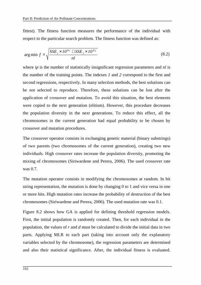
Part II: Prediction of Air Pollutant Concentrations
102
fittest). The fitness function measures the performance of the individual with
respect to the particular search problem. The fitness function was defined as:
nl
10SSE10SSEf
2ip2
1ip1 ×+×
=minarg (8.2)
where ip is the number of statistically insignificant regression parameters and nl is
the number of the training points. The indexes 1 and 2 correspond to the first and
second regressions, respectively. In many selection methods, the best solutions can
be not selected to reproduce. Therefore, these solutions can be lost after the
application of crossover and mutation. To avoid this situation, the best elements
were copied to the next generation (elitism). However, this procedure decreases
the population diversity in the next generations. To reduce this effect, all the
chromosomes in the current generation had equal probability to be chosen by
crossover and mutation procedures.
The crossover operator consists in exchanging genetic material (binary substrings)
of two parents (two chromosomes of the current generation), creating two new
individuals. High crossover rates increase the population diversity, promoting the
mixing of chromosomes (Siriwardene and Perera, 2006). The used crossover rate
was 0.7.
The mutation operator consists in modifying the chromosomes at random. In bit
string representation, the mutation is done by changing 0 to 1 and vice versa in one
or more bits. High mutation rates increase the probability of destruction of the best
chromosomes (Siriwardene and Perera, 2006). The used mutation rate was 0.1.
Figure 8.2 shows how GA is applied for defining threshold regression models.
First, the initial population is randomly created. Then, for each individual in the
population, the values of r and d must be calculated to divide the initial data in two
parts. Applying MLR to each part (taking into account only the explanatory
variables selected by the chromosome), the regression parameters are determined
and also their statistical significance. After, the individual fitness is evaluated.
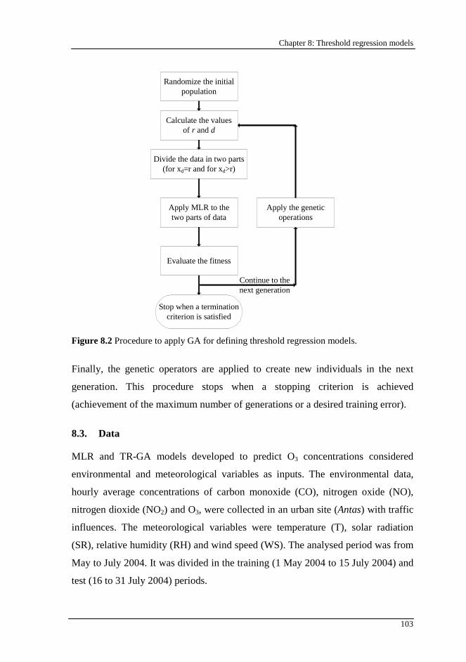
Chapter 8: Threshold regression models
103
Randomize the initial population
Continue to the next generation
Calculate the values of r and d
Divide the data in two parts (for xd=r and for xd>r)
Apply MLR to the two parts of data
Evaluate the fitness
Apply the genetic operations
Stop when a termination criterion is satisfied
Figure 8.2 Procedure to apply GA for defining threshold regression models.
Finally, the genetic operators are applied to create new individuals in the next
generation. This procedure stops when a stopping criterion is achieved
(achievement of the maximum number of generations or a desired training error).
8.3. Data
MLR and TR-GA models developed to predict O3 concentrations considered
environmental and meteorological variables as inputs. The environmental data,
hourly average concentrations of carbon monoxide (CO), nitrogen oxide (NO),
nitrogen dioxide (NO2) and O3, were collected in an urban site (Antas) with traffic
influences. The meteorological variables were temperature (T), solar radiation
(SR), relative humidity (RH) and wind speed (WS). The analysed period was from
May to July 2004. It was divided in the training (1 May 2004 to 15 July 2004) and
test (16 to 31 July 2004) periods.
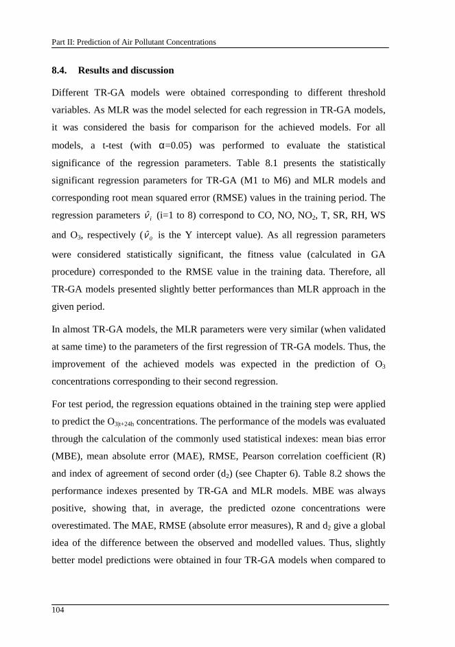
Part II: Prediction of Air Pollutant Concentrations
104
8.4. Results and discussion
Different TR-GA models were obtained corresponding to different threshold
variables. As MLR was the model selected for each regression in TR-GA models,
it was considered the basis for comparison for the achieved models. For all
models, a t-test (with α=0.05) was performed to evaluate the statistical
significance of the regression parameters. Table 8.1 presents the statistically
significant regression parameters for TR-GA (M1 to M6) and MLR models and
corresponding root mean squared error (RMSE) values in the training period. The
regression parameters iν (i=1 to 8) correspond to CO, NO, NO2, T, SR, RH, WS
and O3, respectively ( 0ν is the Y intercept value). As all regression parameters
were considered statistically significant, the fitness value (calculated in GA
procedure) corresponded to the RMSE value in the training data. Therefore, all
TR-GA models presented slightly better performances than MLR approach in the
given period.
In almost TR-GA models, the MLR parameters were very similar (when validated
at same time) to the parameters of the first regression of TR-GA models. Thus, the
improvement of the achieved models was expected in the prediction of O3
concentrations corresponding to their second regression.
For test period, the regression equations obtained in the training step were applied
to predict the O3|t+24h concentrations. The performance of the models was evaluated
through the calculation of the commonly used statistical indexes: mean bias error
(MBE), mean absolute error (MAE), RMSE, Pearson correlation coefficient (R)
and index of agreement of second order (d2) (see Chapter 6). Table 8.2 shows the
performance indexes presented by TR-GA and MLR models. MBE was always
positive, showing that, in average, the predicted ozone concentrations were
overestimated. The MAE, RMSE (absolute error measures), R and d2 give a global
idea of the difference between the observed and modelled values. Thus, slightly
better model predictions were obtained in four TR-GA models when compared to
Chapter 8: Threshold regression models
105
Table 8.1 Statistically significant regression parameters for TR-GA (M1 to M6) and MLR models and correspondent RMSE value in the training data
0ν 1ν 2ν 3ν 4ν 5ν 6ν 7ν 8ν RMSE
42.1 1.7 -4.1 8.5 3.6 3.2 17.8 0.23≤Tif M1
22.6 -8.3 8.5 22.4 5.3 9.0 0.23>Tif
19.9
43.5 2.1 4.5 2.4 4.5 15.1 0.82≤RHif M2
26.8 -5.4 14.5 3.7 13.7 17.2 0.82>RHif
20.0
41.2 -3.9 7.3 6.1 5.4 12.5 0.753 ≤Oif M3
77.2 16.4 10.6 0.753 >Oif
20.0
43.7 2.6 -5.1 8.2 3.5 -5.3 3.0 14.2 3.722 ≤NOif M4
40.2 -6.9 6.9 5.1 8.4 6.0 3.722 >NOif
20.1
12.5 8.4 5.3 -15.6 4.6 10.0 7.55≤RHif M5
43.3 1.7 -3.8 7.0 3.3 -3.9 3.4 14.9 7.55>RHif
20.1
57.5 23.9 5.4 4.9 2.2 -4.0 4.3 15.7 4.304≤COif M6
44.7 -2.8 4.3 3.1 -2.2 3.8 14.4 4.304>COif
20.1
MLR 42.6 -2.2 5.3 3.9 -3.7 3.5 13.9 20.7
Table 8.2 Performance indexes of the TR-GA and MLR models in the test period
Model MBE MAE RMSE R d 2
M1 0.31 15.42 19.66 0.74 0.83 M2 1.61 15.63 19.77 0.74 0.83 M3 0.81 15.92 20.68 0.71 0.81 M4 0.14 16.01 20.94 0.70 0.80 M5 0.43 15.51 19.98 0.73 0.81 M6 1.66 15.45 19.80 0.74 0.83
MLR 0.25 15.59 20.29 0.73 0.81
MLR. The TR-GA1 model presented the best results in both training and test
periods. Figure 8.1 shows the codification of the correspondent chromosome. This
model assumed that the O3|t+24h behaviour changed at the temperature of 23 ºC. For
temperatures below 23 ºC, O3|t+24h depended on CO, NO, NO2, SR, WS and O3,
while for higher values, it depended on CO, NO, T, WS and O3.
The main differences of the regressions in M1 model were the incorporation of
NO2 concentrations and SR as important variables in O3 formation for
Part II: Prediction of Air Pollutant Concentrations
106
temperatures below 23 ºC, being T only important for temperatures above this
threshold value. These observations could be explained by the relative influence of
volatile organic compounds (VOC) and nitrogen oxides (NOx) in O3 formation.
Seinfeld and Pandis (1998) presented the complex chemical reactions involved in
this system and showed that there is a competition between VOC and NOx for the
hydroxyl radical (OH), very important in the O3 formation. At high VOC to NOx
ratio, OH reacts with VOC; otherwise, the NOx reaction predominates. In general,
increasing VOC concentrations means the appearance of more ozone. The effect
of NOx concentration increase depends on the VOC to NOx ratio (positive
correlation for high ratios and negative correlation for low ratios) (Seinfeld and
Pandis, 1998). The temperature has a great influence on O3 formation. High
temperatures favour VOC to NOx ratio because VOC concentrations increase more
with temperature than NOx concentrations. Accordingly, the results showed that
temperature increase lead to higher O3 concentrations (positive correlation
between O3 concentrations and temperature was observed in the second regression
of M1). Simultaneously, as expected, a positive correlation between NO and O3
concentrations was also observed. At lower temperatures, VOC to NOx ratio
decrease and O3 concentrations are greatly dependent on NOx concentrations. As
the correspondent chemical reactions are catalysed by solar radiation (Seinfeld and
Pandis, 1998), this variable was considered statistically significant in the first
regression of M1, presenting a positive correlation with O3 concentrations.
Furthermore, as expected for lower VOC to NOx ratio, a negative correlation
between NO and O3 concentrations was observed.
8.5. Conclusions
GA was applied to define threshold regression models for prediction of the next
day hourly average O3 concentrations. These models assume that the dependent
variable changes its behaviour when an explanatory variable takes a specific value.
Applying the procedure presented in this study, different TR-GA models were
obtained corresponding to different threshold variables and threshold values. In

Chapter 8: Threshold regression models
107
both training and test periods, four of these models presented slightly better results
than MLR approach. Additionally, the best model showed that O3|t+24h changed its
behaviour at the temperature of 23 ºC. For temperatures below that value, O3|t+24h
depended of CO, NO, NO2, SR, WS and O3, while for higher temperatures, it
depended of CO, NO, T, WS and O3.

109
Chapter 9
9. Genetic Programming
This chapter shows how genetic programming can be applied to predict the next day hourly average O3 concentrations. Due to the complexity of this problem, genetic programming is an adequate methodology as it can optimize, simultaneously, the structure of the model and its parameters. It is an artificial intelligence methodology that uses the same principles of the Darwinian Theory of Evolution. Genetic programming enables the automatic generation of mathematical expressions that are modified following an iterative process applying genetic operations.
The contents of this chapter were adapted from: Pires, J.C.M., Alvim-Ferraz, M.C.M., Pereira, M.C., Martins, F.G., 2009. Prediction of Tropospheric Ozone Concentrations: Application of a Methodology Based on the Darwin’s Theory of Evolution. Submitted for publication.
9.1. Introduction
The formation of O3 is a complex, nonlinear, time and space varying process.
Accordingly, several studies presented different statistical approaches to predict
O3 concentrations (Al-Alawi et al., 2008; Coman et al., 2008; Omidvari et al.,
2008; Pires et al., 2008c; Sousa et al., 2006, 2007, 2009), including linear and
nonlinear models. The applied linear models found in the literature were: (i)
multiple linear regression; (ii) principal component regression; (iii) quantile
regression; and (iv) time series. On the other hand, the most common nonlinear
model was the artificial neural network. The selection of a model must consider
some features, such as, complexity, flexibility, accuracy and speed of computation
(Pires et al., 2008d). Artificial neural network models usually presented better
Part II: Prediction of Air Pollutant Concentrations
110
performance than the linear ones (Al-Alawi et al., 2008; Sousa et al., 2006, 2007)
due to the nonlinearity behaviour associated to the O3 formation. However, they
are included in a group called black box models, having limited interpretation.
Moreover, the selection of the optimal network architecture and the computation
time are the main disadvantages of these models.
Besides the structure, the success of a statistical model depends of several factors:
(i) the data size; (ii) the method to optimize their parameters; (iii) the input
variables; and (iv) the collinearity between the input variables. The collinearity
between the input variables can be eliminated through the application of principal
component analysis (see Chapter 6).
As many factors could influence the performance of models, their development
should have more degrees of freedom. For the models referred above, their
structure is fixed in advance and only the parameters are optimized. In stochastic
processes, such as the prediction of O3 concentrations, the structure of the models
should be more flexible. In this context, genetic programming (GP) could be a
successful methodology, as it does not assume in advance any structure for the
model. GP can optimize both the structure of the model and its parameters,
simultaneously. As far as it is known, no study was published applying GP for
predicting air pollutant concentrations. This study aims to predict the next day
hourly average O3 concentrations applying GP to the original input variables and
their correspondent principal components.
9.2. Genetic programming
Genetic programming is an artificial intelligence methodology that uses principles
of the Darwin’s Theory of Evolution. Its search strategy is based on genetic
algorithms (GAs) introduced by John Holland in the 1960s (Goldberg, 1989). GAs
use bit strings as chromosomes and are commonly applied in function
optimization. This algorithm has several disadvantages, for example, the length of
the strings is static (Koza, 1992). Additionally, the size and the shape of the
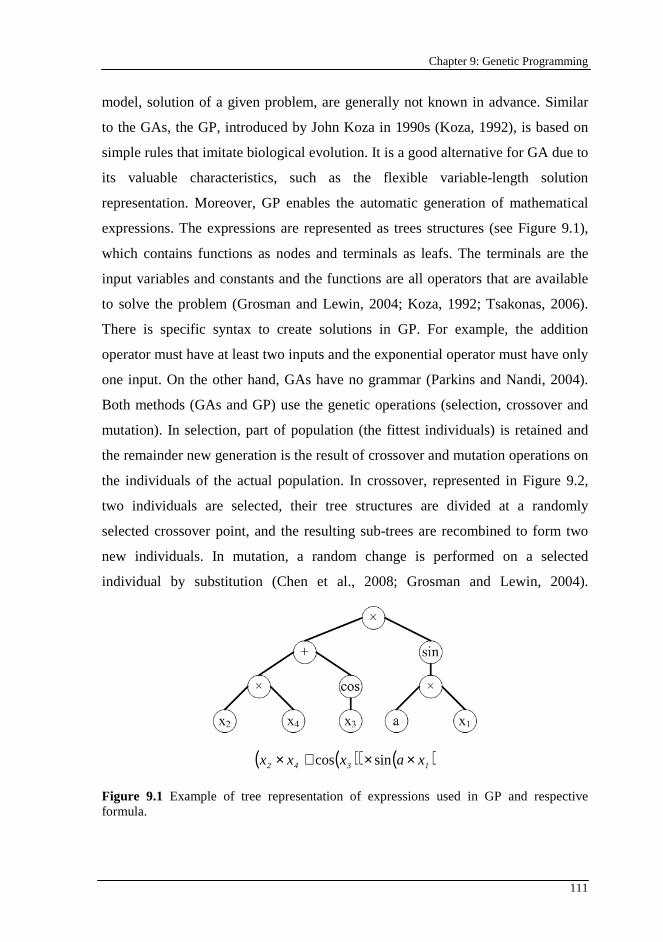
Chapter 9: Genetic Programming
111
model, solution of a given problem, are generally not known in advance. Similar
to the GAs, the GP, introduced by John Koza in 1990s (Koza, 1992), is based on
simple rules that imitate biological evolution. It is a good alternative for GA due to
its valuable characteristics, such as the flexible variable-length solution
representation. Moreover, GP enables the automatic generation of mathematical
expressions. The expressions are represented as trees structures (see Figure 9.1),
which contains functions as nodes and terminals as leafs. The terminals are the
input variables and constants and the functions are all operators that are available
to solve the problem (Grosman and Lewin, 2004; Koza, 1992; Tsakonas, 2006).
There is specific syntax to create solutions in GP. For example, the addition
operator must have at least two inputs and the exponential operator must have only
one input. On the other hand, GAs have no grammar (Parkins and Nandi, 2004).
Both methods (GAs and GP) use the genetic operations (selection, crossover and
mutation). In selection, part of population (the fittest individuals) is retained and
the remainder new generation is the result of crossover and mutation operations on
the individuals of the actual population. In crossover, represented in Figure 9.2,
two individuals are selected, their tree structures are divided at a randomly
selected crossover point, and the resulting sub-trees are recombined to form two
new individuals. In mutation, a random change is performed on a selected
individual by substitution (Chen et al., 2008; Grosman and Lewin, 2004).
( )( ) ( )1342 xaxxx ××+× sincos
Figure 9.1 Example of tree representation of expressions used in GP and respective formula.
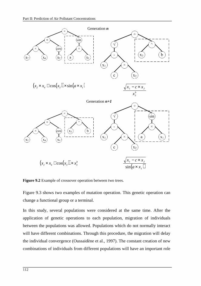
Part II: Prediction of Air Pollutant Concentrations
112
( )( ) ( )1342 xaxxx ××+× sincos b3
21
x
xcx ×−
( )( ) b3342 xxxx ×+× cos ( )1
21
xa
xcx
××−
sin
Figure 9.2 Example of crossover operation between two trees.
Figure 9.3 shows two examples of mutation operation. This genetic operation can
change a functional group or a terminal.
In this study, several populations were considered at the same time. After the
application of genetic operations to each population, migration of individuals
between the populations was allowed. Populations which do not normally interact
will have different combinations. Through this procedure, the migration will delay
the individual convergence (Oussaidène et al., 1997). The constant creation of new
combinations of individuals from different populations will have an important role
Generation n+1
Generation n
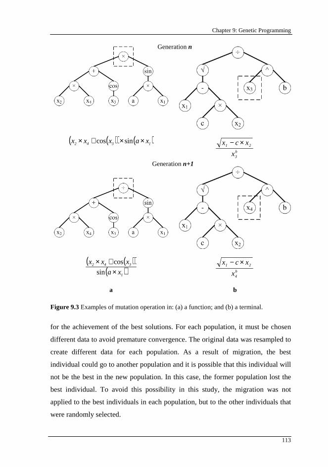
Chapter 9: Genetic Programming
113
( )( ) ( )1342 xaxxx ××+× sincos b3
21
x
xcx ×−
( )( )( )1
342
xa
xxx
×+×
sin
cos
b4
21
x
xcx ×−
a b
Figure 9.3 Examples of mutation operation in: (a) a function; and (b) a terminal.
for the achievement of the best solutions. For each population, it must be chosen
different data to avoid premature convergence. The original data was resampled to
create different data for each population. As a result of migration, the best
individual could go to another population and it is possible that this individual will
not be the best in the new population. In this case, the former population lost the
best individual. To avoid this possibility in this study, the migration was not
applied to the best individuals in each population, but to the other individuals that
were randomly selected.
Generation n
Generation n+1
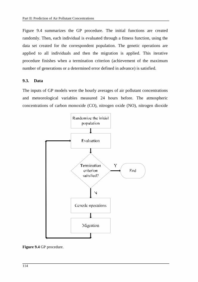
Part II: Prediction of Air Pollutant Concentrations
114
Figure 9.4 summarizes the GP procedure. The initial functions are created
randomly. Then, each individual is evaluated through a fitness function, using the
data set created for the correspondent population. The genetic operations are
applied to all individuals and then the migration is applied. This iterative
procedure finishes when a termination criterion (achievement of the maximum
number of generations or a determined error defined in advance) is satisfied.
9.3. Data
The inputs of GP models were the hourly averages of air pollutant concentrations
and meteorological variables measured 24 hours before. The atmospheric
concentrations of carbon monoxide (CO), nitrogen oxide (NO), nitrogen dioxide
Figure 9.4 GP procedure.
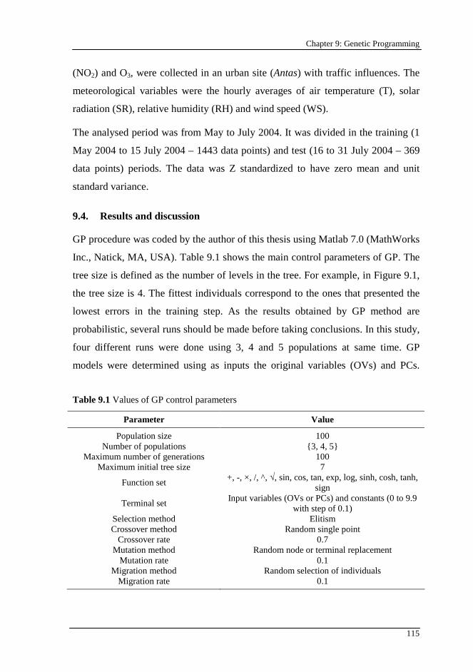
Chapter 9: Genetic Programming
115
(NO2) and O3, were collected in an urban site (Antas) with traffic influences. The
meteorological variables were the hourly averages of air temperature (T), solar
radiation (SR), relative humidity (RH) and wind speed (WS).
The analysed period was from May to July 2004. It was divided in the training (1
May 2004 to 15 July 2004 – 1443 data points) and test (16 to 31 July 2004 – 369
data points) periods. The data was Z standardized to have zero mean and unit
standard variance.
9.4. Results and discussion
GP procedure was coded by the author of this thesis using Matlab 7.0 (MathWorks
Inc., Natick, MA, USA). Table 9.1 shows the main control parameters of GP. The
tree size is defined as the number of levels in the tree. For example, in Figure 9.1,
the tree size is 4. The fittest individuals correspond to the ones that presented the
lowest errors in the training step. As the results obtained by GP method are
probabilistic, several runs should be made before taking conclusions. In this study,
four different runs were done using 3, 4 and 5 populations at same time. GP
models were determined using as inputs the original variables (OVs) and PCs.
Table 9.1 Values of GP control parameters
Parameter Value
Population size 100 Number of populations {3, 4, 5}
Maximum number of generations 100 Maximum initial tree size 7
Function set +, -, ×, /, ^, √, sin, cos, tan, exp, log, sinh, cosh, tanh,
sign
Terminal set Input variables (OVs or PCs) and constants (0 to 9.9
with step of 0.1) Selection method Elitism Crossover method Random single point
Crossover rate 0.7 Mutation method Random node or terminal replacement
Mutation rate 0.1 Migration method Random selection of individuals
Migration rate 0.1
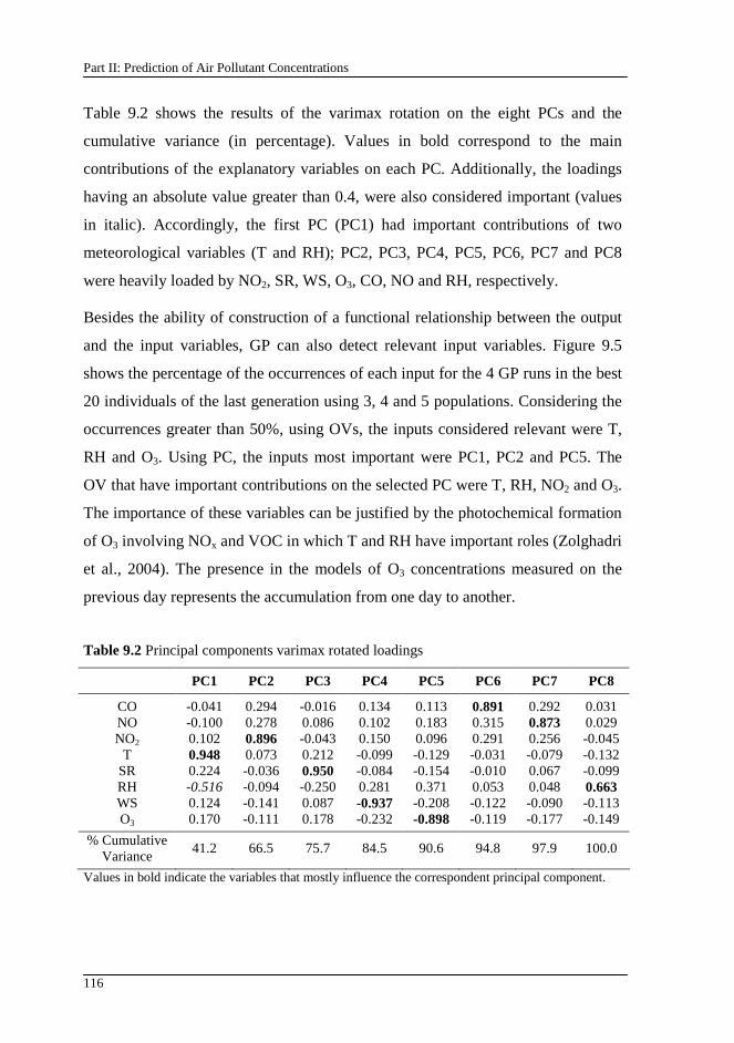
Part II: Prediction of Air Pollutant Concentrations
116
Table 9.2 shows the results of the varimax rotation on the eight PCs and the
cumulative variance (in percentage). Values in bold correspond to the main
contributions of the explanatory variables on each PC. Additionally, the loadings
having an absolute value greater than 0.4, were also considered important (values
in italic). Accordingly, the first PC (PC1) had important contributions of two
meteorological variables (T and RH); PC2, PC3, PC4, PC5, PC6, PC7 and PC8
were heavily loaded by NO2, SR, WS, O3, CO, NO and RH, respectively.
Besides the ability of construction of a functional relationship between the output
and the input variables, GP can also detect relevant input variables. Figure 9.5
shows the percentage of the occurrences of each input for the 4 GP runs in the best
20 individuals of the last generation using 3, 4 and 5 populations. Considering the
occurrences greater than 50%, using OVs, the inputs considered relevant were T,
RH and O3. Using PC, the inputs most important were PC1, PC2 and PC5. The
OV that have important contributions on the selected PC were T, RH, NO2 and O3.
The importance of these variables can be justified by the photochemical formation
of O3 involving NOx and VOC in which T and RH have important roles (Zolghadri
et al., 2004). The presence in the models of O3 concentrations measured on the
previous day represents the accumulation from one day to another.
Table 9.2 Principal components varimax rotated loadings
PC1 PC2 PC3 PC4 PC5 PC6 PC7 PC8
CO -0.041 0.294 -0.016 0.134 0.113 0.891 0.292 0.031 NO -0.100 0.278 0.086 0.102 0.183 0.315 0.873 0.029 NO2 0.102 0.896 -0.043 0.150 0.096 0.291 0.256 -0.045
T 0.948 0.073 0.212 -0.099 -0.129 -0.031 -0.079 -0.132 SR 0.224 -0.036 0.950 -0.084 -0.154 -0.010 0.067 -0.099 RH -0.516 -0.094 -0.250 0.281 0.371 0.053 0.048 0.663 WS 0.124 -0.141 0.087 -0.937 -0.208 -0.122 -0.090 -0.113 O3 0.170 -0.111 0.178 -0.232 -0.898 -0.119 -0.177 -0.149
% Cumulative Variance
41.2 66.5 75.7 84.5 90.6 94.8 97.9 100.0
Values in bold indicate the variables that mostly influence the correspondent principal component.
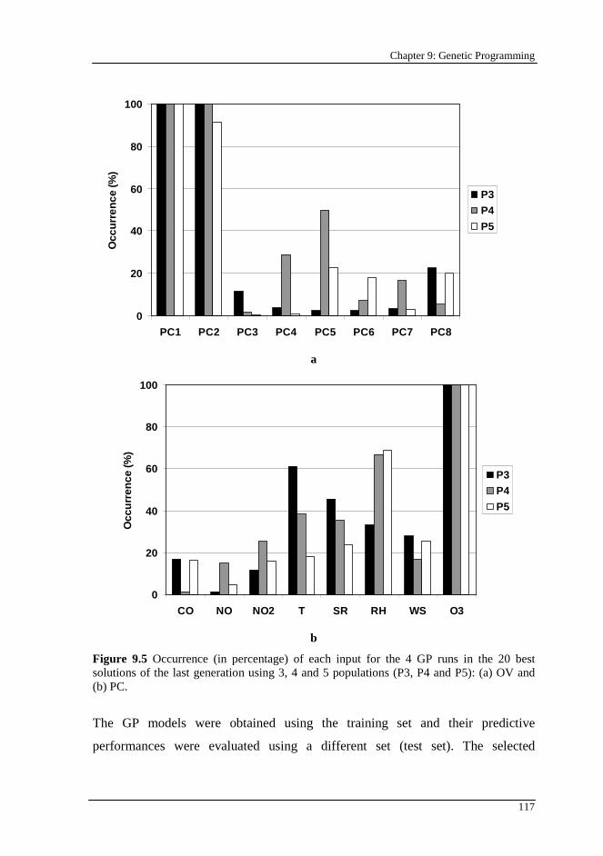
Chapter 9: Genetic Programming
117
0
20
40
60
80
100
PC1 PC2 PC3 PC4 PC5 PC6 PC7 PC8
Occ
urr
ence
(%)
P3
P4
P5
a
0
20
40
60
80
100
CO NO NO2 T SR RH WS O3
Occ
urr
ence
(%)
P3
P4
P5
b
Figure 9.5 Occurrence (in percentage) of each input for the 4 GP runs in the 20 best solutions of the last generation using 3, 4 and 5 populations (P3, P4 and P5): (a) OV and (b) PC.
The GP models were obtained using the training set and their predictive
performances were evaluated using a different set (test set). The selected
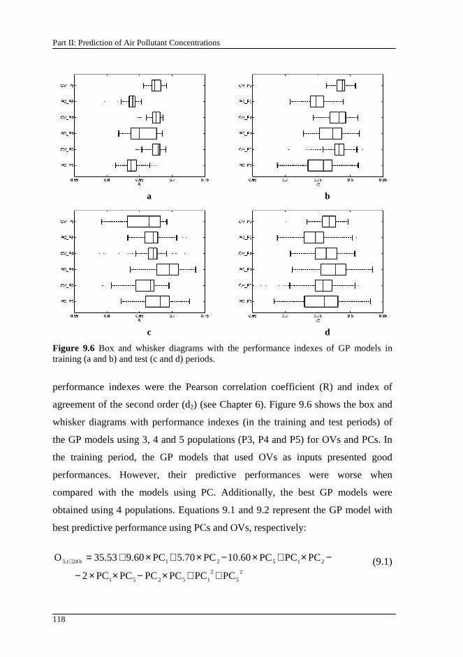
Part II: Prediction of Air Pollutant Concentrations
118
a b
c d
Figure 9.6 Box and whisker diagrams with the performance indexes of GP models in training (a and b) and test (c and d) periods.
performance indexes were the Pearson correlation coefficient (R) and index of
agreement of the second order (d2) (see Chapter 6). Figure 9.6 shows the box and
whisker diagrams with performance indexes (in the training and test periods) of
the GP models using 3, 4 and 5 populations (P3, P4 and P5) for OVs and PCs. In
the training period, the GP models that used OVs as inputs presented good
performances. However, their predictive performances were worse when
compared with the models using PC. Additionally, the best GP models were
obtained using 4 populations. Equations 9.1 and 9.2 represent the GP model with
best predictive performance using PCs and OVs, respectively:
2
5
2
15251
21521h24t3,
PCPCPCPCPCPC2
PCPCPC10.60PC5.70PC9.6035.53O
++×−××−
−×+×−×+×+=+ (9.1)
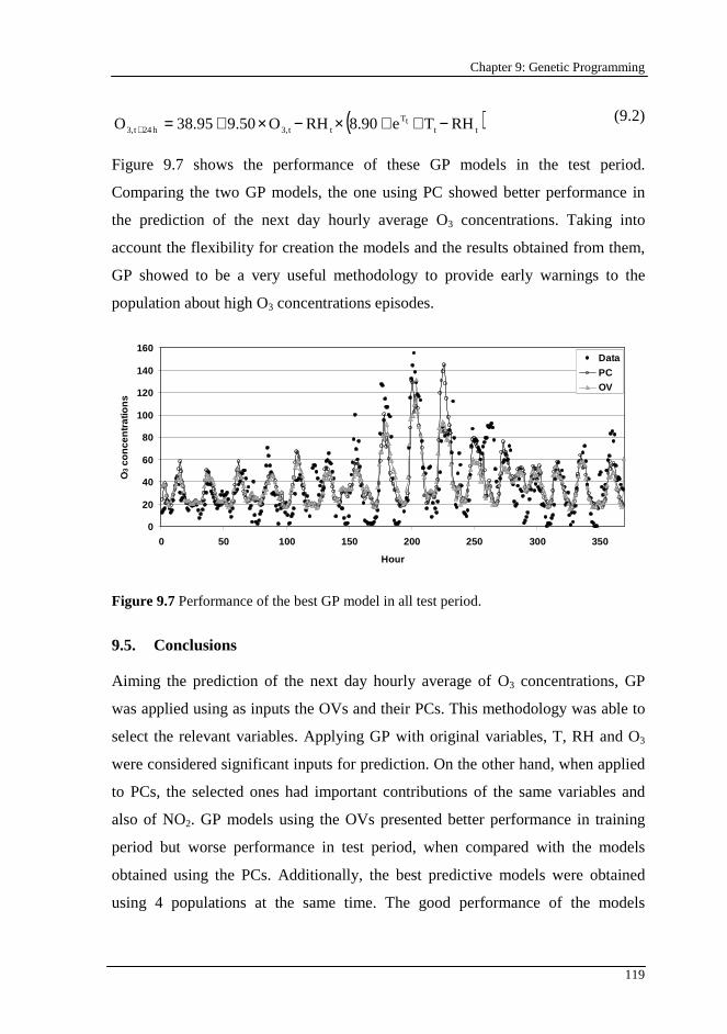
Chapter 9: Genetic Programming
119
( )tttT
tt3,h24t3, RHTe8.90RHO9.5038.95O −++×−×+=+ (9.2)
Figure 9.7 shows the performance of these GP models in the test period.
Comparing the two GP models, the one using PC showed better performance in
the prediction of the next day hourly average O3 concentrations. Taking into
account the flexibility for creation the models and the results obtained from them,
GP showed to be a very useful methodology to provide early warnings to the
population about high O3 concentrations episodes.
0
20
40
60
80
100
120
140
160
0 50 100 150 200 250 300 350
Hour
O3
con
cen
trat
ion
s
Data
PCOV
Figure 9.7 Performance of the best GP model in all test period.
9.5. Conclusions
Aiming the prediction of the next day hourly average of O3 concentrations, GP
was applied using as inputs the OVs and their PCs. This methodology was able to
select the relevant variables. Applying GP with original variables, T, RH and O3
were considered significant inputs for prediction. On the other hand, when applied
to PCs, the selected ones had important contributions of the same variables and
also of NO2. GP models using the OVs presented better performance in training
period but worse performance in test period, when compared with the models
obtained using the PCs. Additionally, the best predictive models were obtained
using 4 populations at the same time. The good performance of the models

Part II: Prediction of Air Pollutant Concentrations
120
associated to the facility to achieve them showed that GP can be very useful to
solve several environmental complex problems.

121
Chapter 10
10. Multi-gene Genetic Programming
This chapter aims to apply a multi-gene genetic programming methodology for predicting the daily average of PM10 concentrations on the next day. This methodology is based on the principles of the simple genetic programming algorithm. The models are also encoded in tree structures that are modified following an iterative process; the model structure and parameters are optimized at same time. The main differences between the simple and the multi-gene genetic programming methodologies are: (i) an individual is composed by several tree structures, called genes, and not a single one; and (ii) the output value is calculated through the linear combination of the outputs of the different genes belonging to the same individual.
The contents of this chapter were adapted from: Pires, J.C.M., Alvim-Ferraz, M.C.M., Pereira, M.C., Martins, F.G., 2009. A Multi-Gene Genetic Programming Methodology to Generate Models for Predicting the Daily Average of PM10 Concentrations, submitted for publication.
10.1. Introduction
The choice of a model for any case study occurs in different steps in which the
first one is the selection between the two main classes: mechanistic and
phenomenological models. The mechanistic models are more concerned with the
underlying processes (physical, chemical and biological processes), using
functions based on theoretical expectations (Bolker, 2008). On the other hand,
phenomenological models are concentrated on observed patterns in the data, using
functions that organize the experimental observations within a formal structure.
The use of phenomenological models has become increasingly recommended for
applications where the mechanistic description of the interdependence between
Part II: Prediction of Air Pollutant Concentrations
122
variables is either unknown or very complex. The prediction of air pollutant
concentrations is a complex problem and, specifically for PM10, phenomenological
models are particularly attractive, due to the complexity of the involved processes
(Corani, 2005; Perez and Reyes, 2002; Fuller et al., 2002; Pires et al., 2008d).
The studies presented in Chapter 5 showed that the structure definition is an
important step for the model success, being followed by the optimization of its
parameters. In all studies aiming the prediction of PM10 concentrations, the
structures of the models were defined in advance and after the parameters were
determined minimizing an objective function. As PM10 concentrations are highly
influenced by stochastic processes (such as meteorological effects, dry deposition
and chemical reaction), the determination of the model should be done optimizing
the model structure and parameters simultaneously. Thus, this study aims to
predict the daily average of PM10 concentrations optimizing the model structure
and parameters simultaneously, using multi-gene genetic programming (MGP). As
far it is known, no study was presented applying MGP for the prediction of PM10
concentrations.
MGP follows the same principles of genetic programming described in Chapter 9.
It is a method that predicts the output variable through the weighted linear
combination of the outputs from several symbolic tree structures that correspond
to the different genes. The weights are determined by minimizing the sum of
squared errors of the predicted values.
10.2. Data
The variables selected as PM10 predictors were the concentrations of several air
pollutants (SO2, CO, NO, NO2 and PM10) and meteorological variables (air
temperature - T; relative humidity – RH; and wind speed - WS). The
concentrations of pollutants were recorded in an urban site (Matosinhos) with
traffic influences. Daily average values for these variables were calculated and
used if more than 75% of hourly averages were available.
Chapter 10: Multi-gene Genetic Programming
123
The period of measurement (from January 2003 to December 2005) was divided in
training and test periods. The training data were used to determine the MGP
models and the test data were used to evaluate the performance of application to a
new set. The test data corresponded to the last quarter of 2005 (76 data points),
considering training data the remaining period (914 data points). The explanatory
variables were Z standardized to have zero mean and unit standard deviation.
10.3. Results and discussion
The MGP algorithm was coded in Matlab 7.0 (MathWorks Inc., Natick, MA,
USA) by the author of this thesis. Several parameters must be defined for the MGP
approach. In this study, the population size was fixed to 200. The maximum
number of generations was 100. The crossover and mutation rates define the
probability that an individual is selected for the crossover or mutation operation,
respectively; their values were 0.8 and 0.1. The 10% of the best individuals (20
individuals) were selected for the next generation (elitism). The fittest individuals
were the ones presenting the lowest root mean squared error (RMSE) in the
training period. To avoid early convergence, a new dataset for the evaluation of
individuals was created, by random sampling the original data, with replacement
when the 20 best individuals of the actual generation were the same of the
previous one. However, in the last 10 generations the individuals were evaluated
using the original data. Since the MGP results are probabilistic, several MGP runs
of the algorithm must be performed and their results analysed before taking
conclusions. Ten MGP runs were done with the individuals composed by five
genes. The predicted PM10 concentrations were calculated through the linear
combination of the outputs from the five correspondent tree expressions.
Besides the ability of construction of a functional relationship between the output
and the input variables, MGP also detects the relevant inputs. Figure 10.1 shows
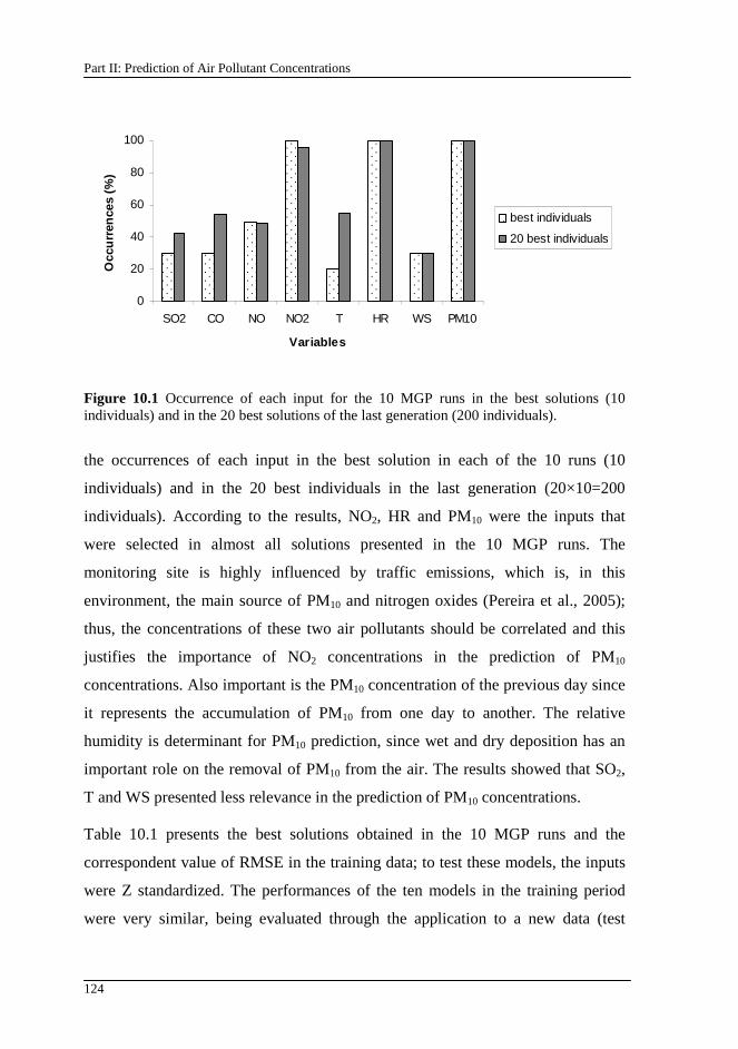
Part II: Prediction of Air Pollutant Concentrations
124
0
20
40
60
80
100
SO2 CO NO NO2 T HR WS PM10
Variables
Occ
urr
ence
s (%
)
best individuals
20 best individuals
Figure 10.1 Occurrence of each input for the 10 MGP runs in the best solutions (10 individuals) and in the 20 best solutions of the last generation (200 individuals).
the occurrences of each input in the best solution in each of the 10 runs (10
individuals) and in the 20 best individuals in the last generation (20×10=200
individuals). According to the results, NO2, HR and PM10 were the inputs that
were selected in almost all solutions presented in the 10 MGP runs. The
monitoring site is highly influenced by traffic emissions, which is, in this
environment, the main source of PM10 and nitrogen oxides (Pereira et al., 2005);
thus, the concentrations of these two air pollutants should be correlated and this
justifies the importance of NO2 concentrations in the prediction of PM10
concentrations. Also important is the PM10 concentration of the previous day since
it represents the accumulation of PM10 from one day to another. The relative
humidity is determinant for PM10 prediction, since wet and dry deposition has an
important role on the removal of PM10 from the air. The results showed that SO2,
T and WS presented less relevance in the prediction of PM10 concentrations.
Table 10.1 presents the best solutions obtained in the 10 MGP runs and the
correspondent value of RMSE in the training data; to test these models, the inputs
were Z standardized. The performances of the ten models in the training period
were very similar, being evaluated through the application to a new data (test
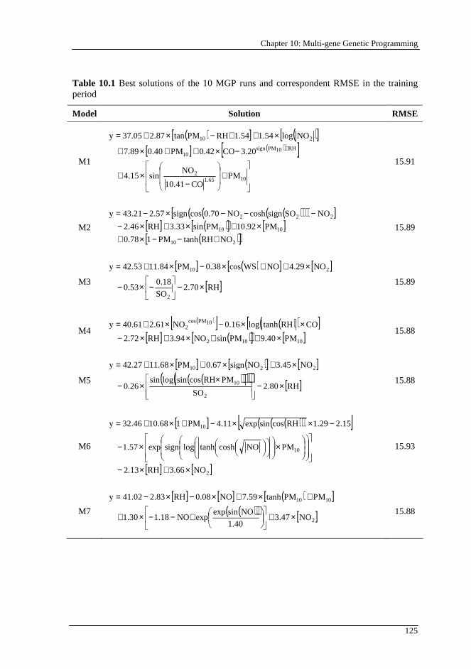
Chapter 10: Multi-gene Genetic Programming
125
Table 10.1 Best solutions of the 10 MGP runs and correspondent RMSE in the training period
Model Solution RMSE
M1
( )[ ] ( )[ ][ ] ( )[ ]
+
−×+
−×++×+
×++−×+=+
101.652
RH10PMsign10
210
PMCO10.41
NOsin4.15
3.20CO0.42PM0.407.89
NOlog1.541.54RHPMtan2.8737.05y
15.91
M2
( )( )( )( )[ ][ ] ( )[ ] [ ]
( )[ ]210
1010
222
NORHtanhPM10.78
PM10.92PMsin3.33RH2.46
NOSOsigncoshNO0.70cossign2.5743.21y
+−−×+×+×+×−
−−−×−= 15.89
M3
[ ] ( )[ ] [ ]
[ ]RH2.70SO
0.180.53
NO4.29NOWScos0.38PM11.8442.53y
2
210
×−
−×−
×++×−×+=
15.89
M4 ( )[ ] ( )( )[ ]
[ ] ( )[ ] [ ]10102
10PMcos2
PM9.40PMsinNO3.94RH2.72
CORHtanhlog0.16NO2.6140.61y
×++×+×−
××−×+= 15.88
M5
[ ] ( )[ ] [ ]( )( )( )( ) [ ]RH2.80
SO
PMRHcossinlogsin0.26
NO3.45NOsign0.67PM11.6842.27y
2
10
2210
×−
××−
×+×+×+=
15.88
M6
[ ] ( )( )( )[ ]
[ ] [ ]2
10
10
NO3.66RH2.13
PMNOcoshtanhlogsignexp1.57
2.151.29RHcossinexp4.11PM110.6832.46y
×+×−
×
×−
−××−+×+=
15.93
M7
[ ] [ ] ( )[ ]( )( ) [ ]2
1010
NO3.471.40
NOsinexpexpNO1.181.30
PMPMtanh7.59NO0.08RH2.8341.02y
×+
+−−×+
+×+×−×−= 15.88
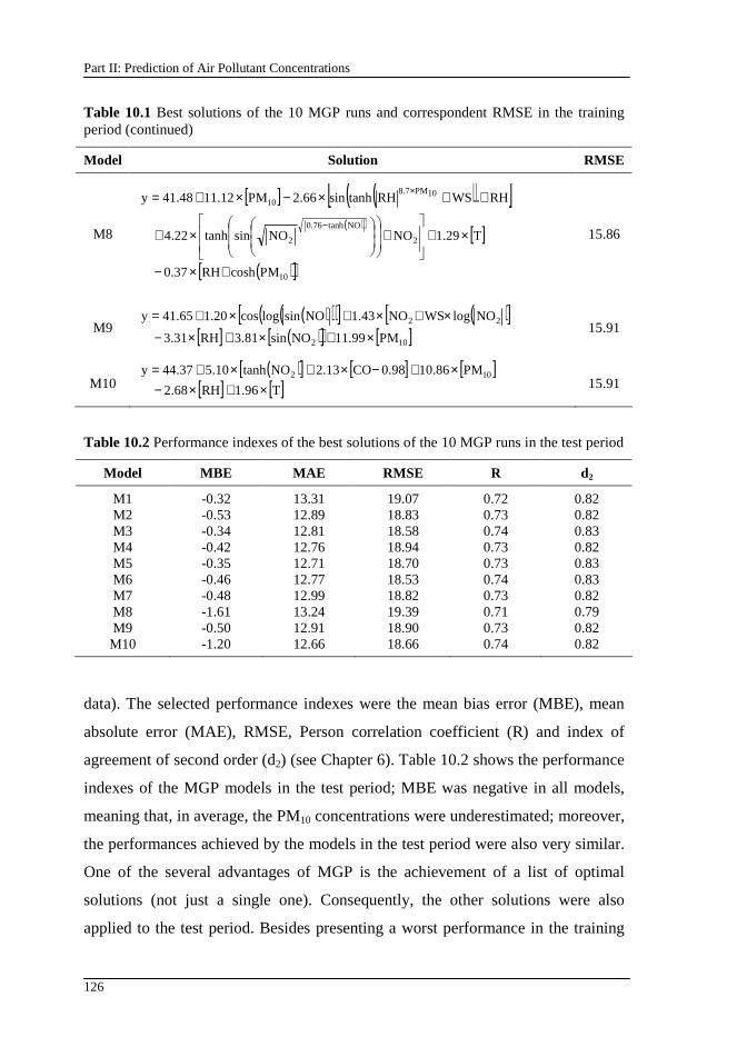
Part II: Prediction of Air Pollutant Concentrations
126
Table 10.1 Best solutions of the 10 MGP runs and correspondent RMSE in the training period (continued)
Model Solution RMSE
M8
[ ] ( )( )[ ]( ) [ ]
( )[ ]10
2
NOtanh0.76
2
10PM8.710
PMcoshRH0.37
T1.29NONOsintanh4.22
RHWSRHtanhsin2.66PM11.1241.48y
+×−
×+
+
×+
++×−×+=
−
×
15.86
M9 ( )( )( )[ ] ( )[ ]
[ ] ( )[ ] [ ]102
22
PM11.99NOsin3.81RH3.31
NOlogWSNO1.43NOsinlogcos1.2041.65y
×+×+×−
×+×+×+= 15.91
M10 ( )[ ] [ ] [ ]
[ ] [ ]T1.96RH2.68
PM10.860.98CO2.13NOtanh5.1044.37y 102
×+×−×+−×+×+=
15.91
Table 10.2 Performance indexes of the best solutions of the 10 MGP runs in the test period
Model MBE MAE RMSE R d 2
M1 -0.32 13.31 19.07 0.72 0.82 M2 -0.53 12.89 18.83 0.73 0.82 M3 -0.34 12.81 18.58 0.74 0.83 M4 -0.42 12.76 18.94 0.73 0.82 M5 -0.35 12.71 18.70 0.73 0.83 M6 -0.46 12.77 18.53 0.74 0.83 M7 -0.48 12.99 18.82 0.73 0.82 M8 -1.61 13.24 19.39 0.71 0.79 M9 -0.50 12.91 18.90 0.73 0.82 M10 -1.20 12.66 18.66 0.74 0.82
data). The selected performance indexes were the mean bias error (MBE), mean
absolute error (MAE), RMSE, Person correlation coefficient (R) and index of
agreement of second order (d2) (see Chapter 6). Table 10.2 shows the performance
indexes of the MGP models in the test period; MBE was negative in all models,
meaning that, in average, the PM10 concentrations were underestimated; moreover,
the performances achieved by the models in the test period were also very similar.
One of the several advantages of MGP is the achievement of a list of optimal
solutions (not just a single one). Consequently, the other solutions were also
applied to the test period. Besides presenting a worst performance in the training
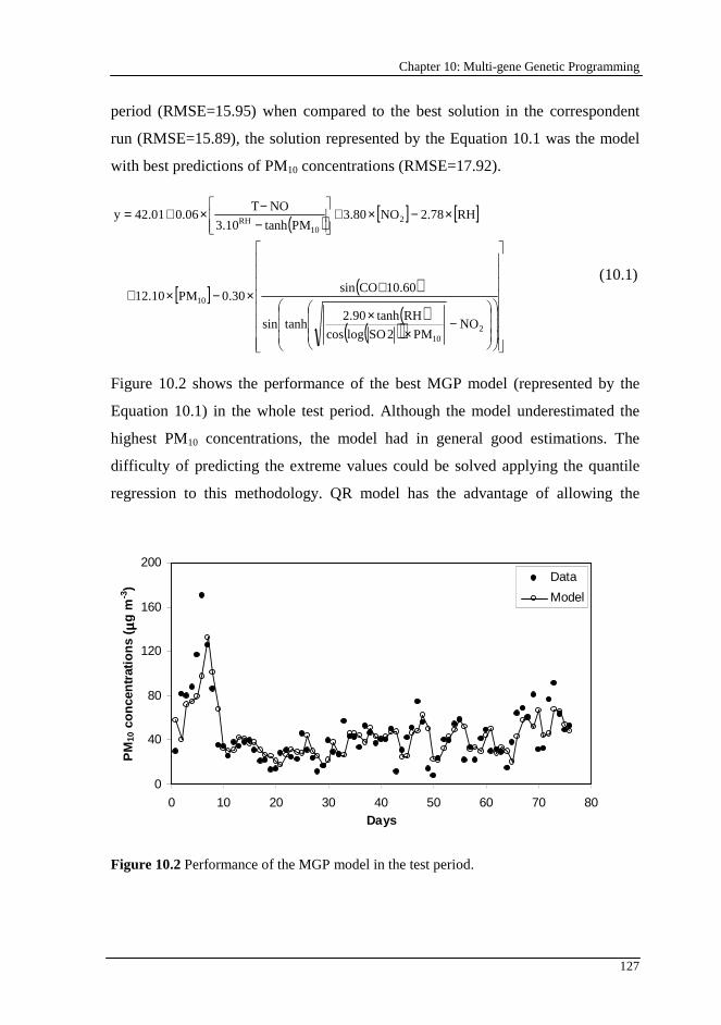
Chapter 10: Multi-gene Genetic Programming
127
period (RMSE=15.95) when compared to the best solution in the correspondent
run (RMSE=15.89), the solution represented by the Equation 10.1 was the model
with best predictions of PM10 concentrations (RMSE=17.92).
( ) [ ] [ ]
[ ] ( )( )
( )( )
−
××
+×−×+
×−×+
−−×+=
210
10
210
RH
NOPM2SOlogcos
RHtanh2.90tanhsin
10.60COsin0.30PM12.10
RH2.78NO3.80PMtanh3.10
NOT0.0642.01y
(10.1)
Figure 10.2 shows the performance of the best MGP model (represented by the
Equation 10.1) in the whole test period. Although the model underestimated the
highest PM10 concentrations, the model had in general good estimations. The
difficulty of predicting the extreme values could be solved applying the quantile
regression to this methodology. QR model has the advantage of allowing the
0
40
80
120
160
200
0 10 20 30 40 50 60 70 80Days
PM
10 c
on
cen
trat
ion
s ( µµ µµ
g m
-3)
Data
Model
Figure 10.2 Performance of the MGP model in the test period.
Part II: Prediction of Air Pollutant Concentrations
128
examination of the entire distribution of the variable of interest rather than
measuring the central tendency of its distribution. For example, Sousa et al. (2009)
compared the performance of MLR and QR in the prediction of tropospheric
ozone concentrations and concluded that QR presented better performance than
MLR especially in the extreme values.
Considering the flexibility for creating the predictive models, MGP is a promising
methodology to estimate environmental complex air pollution problems.
10.4. Conclusions
Aiming the prediction of the daily average of PM10 concentrations on the next day,
MGP was applied. The results showed two important features of MGP: the
selection of the relevant inputs and the construction of the predictive model. The
variables considered important for PM10 concentrations prediction were NO2
concentrations, RH and PM10 concentrations measured in the previous day. MGP
provided several models that presented similar performances indexes. The good
performances of the models showed that MGP is a useful tool to public health
protection as it can provide early warnings to the population about high PM10
concentrations episodes.
129
Chapter 11
11. Final Words
In this thesis, two important issues in the field of air quality management were approached. First, statistical methods were applied to characterize the air pollution behaviours in Oporto-MA, which was followed by the determination of redundant measurements in the air quality monitoring network. Second, the statistical models were developed and applied to predict the O3 and PM10 concentrations. This chapter also proposes future work concerning these two issues.
11.1. General conclusions
The characterization of the air pollution behaviours in Oporto-MA was an
important step to determine redundant measurements in the local air quality
monitoring network. If two different monitoring sites present similar air pollution
behaviour, only one should operate, since the measured values at this monitoring
site are representative for the two regions. With the actual distribution of
monitoring sites, several redundant measurements were identified. The applied
statistical methods were able to determine the patterns on air quality data and to
evaluate the minimum number of monitoring sites that should operate for each air
pollutant. For principal component analysis, two different criteria were applied to
select the number of principal components. Using Kaiser criterion (which is often
applied), the principal components selected did not represent sufficient variance of
the original data. Other criterion, which selects the number of principal
components representing at least 90% of the original data variance, presented
better results, when the concentrations of air pollutants at the removed monitoring
sites were predicted. This means that this method or one that selects principal
Development and Application of Statistical Methods to Support Air Quality Policy Decisions
130
components with more information about the original variables should be applied
for these studies. Accordingly, the number of monitoring sites could be reduced
more than 50% in some of the analysed air pollutants.
The air pollution behaviours are greatly influenced by the relative location of
emission point sources. This was observed for SO2, for which the principal
component analysis determined the existence of at least six monitoring sites (the
highest number selected with Kaiser criterion). The location of emission sources
was determined analysing the variation of air pollutant concentrations with the
wind direction. For SO2, an emission source was identified inside the area defined
by the air quality monitoring network. Thus, for each wind direction, different
places will be affected by the emissions from that source and, for that reason, they
presented different air pollution behaviour.
The statistical methods should be applied using data corresponding to smaller
periods. Longer periods hide seasonal differences in air pollution behaviours
between monitoring sites. In this case, a wrong decision (remove or displace a
monitoring site) can be taken. For example, applying principal component analysis
(using the Kaiser criterion) to the PM10 data of three years, the Vila do Conde site
was grouped with other sites, when this site presented higher concentrations and
different daily profiles of PM10 concentrations. This happens in several periods
from 17 h to 22 h. In the remaining periods, Vila do Conde site had similar PM10
behaviour. The emission source responsible of this difference was identified at N-
NW direction sector. However, this source took less relevance in the last year of
study. Despite this different behaviour, the site was grouped with other sites by the
principal component analysis using Kaiser criterion. Using other criterion for
selection of the number of principal components and analysing smaller periods
(annual quarters), Vila do Conde site belonged to a different group.
In the second part of the thesis, statistical models were developed to predict O3 and
PM10 concentrations. The linear models had an advantage of taking less
computational time than the other models. Taking into account the performance of
Chapter 11: Final Words
131
these models, quantile regression was the best model in the training period, as it
tries to model the entire distribution of the dependent variable. However, this
method presented bad predictive performance. Partial least squares regression was
the linear model with best predictive performance for both air pollutant
concentrations.
Until now, no study was presented aiming the prediction of air pollutant
concentrations through statistical models using independent components.
Independent component regression and stepwise artificial neural networks (using
independent components as inputs) were applied. However, both models presented
bad performances.
The recommended statistical approaches to solve stochastic problems, such as
prediction of air pollutant concentrations, were the ones using the evolutionary
procedure. They presented the best predictive performances for both air pollutants:
(i) threshold regression using genetic algorithms and genetic programming for O3;
and (ii) multi-gene genetic programming for PM10. They have the advantage of not
defining the model structure in advance. The model structure and parameters were
optimized simultaneously. The threshold regression, which was applied to predict
O3 concentrations, assumed different relationships between the O3 concentrations
and their precursors. This is important for this air pollutant, as it is formed by
chemical reactions that are influenced by different regimes. In this study, only two
regression equations were applied (assuming two regimes). This method is also
similar to quantile regression with the advantage that it is not needed to predict the
percentile of the output variable.
The accuracy of the predictions from statistical models is a function of the quality
of the data in the various databases. The lack of adequate data on air pollutant
concentrations is a major limitation of the statistical methods. When the data
needed to drive the models are available, the models provide policy makers with
useful information on the exposure of the population to air pollutants.
Development and Application of Statistical Methods to Support Air Quality Policy Decisions
132
11.2. Future work
Concerning the management of the equipment of the air quality monitoring
networks, the method to evaluate redundant measurements was tested and
presented adequate results. After the selection of redundant monitoring sites, the
correspondent equipment can be displaced to other regions increasing the
monitored area. The location of new monitoring sites can be determined using a
mobile air quality monitoring equipment. Using this equipment, the air pollutant
concentrations should be measured in a determined place during sufficient large
period. Principal component analysis should be applied to data of the fixed and
mobile monitoring sites. If the place presents different air pollution behaviour
from other regions, it should have a monitoring site.
Concerning the prediction of air pollutant concentrations, the data size should be
reduced. It was observed that the models have difficulties to predict extreme
values, tending for the average value of the training data. The data corresponding a
large period contain different relationships between variables, which is difficult to
model in only one equation. The reduction of the data size also decreases the
computation time to achieve the statistical models. Additionally, it is important to
explore the potentialities of the threshold regression. This model could be applied
assuming more than two equations and also non-linear relationships between input
and output variables in each regime. In this case, the codification of chromosomes
in GA should be modified.
To improve the results of these models in the air quality modelling, the objective
function could also be changed. In air quality modelling, it is not important to
know the exact concentrations of the air pollutant, but to predict the range of
values that will limit these concentrations. An example of an objective function
that can be applied in this field is the minimization of the sum of absolute errors,
when the absolute error is greater than a defined value.
133
References
Abdi, H., 2003. Partial Least Squares (PLS) Regression. In: Encyclopedia of Social
Sciences Research Methods (eds. M. Lewis-Beck, A. Bryman and T. Futing), 1-7.
Thousand Oaks: Sage.
Abdul-Wahab, S.A., Bakheit, C.S., Al-Alawi, S.M., 2005. Principal component and
multiple regression analysis in modelling of ground-level ozone and factors affecting
its concentrations. Environmental Modelling & Software 20 (10), 1263-1271.
Agirre-Basurko, E., Ibarra-Berastegi, G., Madariaga, I., 2006. Regression and multilayer
perceptron-based models to forecast hourly O3 and NO2 levels in the Bilbao area.
Environmental Modelling & Software 21, 430-446.
Al-Alawi, S.M., Abdul-Wahab, S.A., Bakheit, C.S., 2008. Combining principal component
regression and artificial neural networks for more accurate predictions of ground-
level ozone. Environmental Modelling & Software 23(4), 396-403.
Al-Rubaie, K.S., Godefroid, L.B., Lopes, J.A.M., 2007. Statistical modeling of fatigue
crack growth rate in Inconel alloy 600. International Journal of Fatigue 29 (5), 931-
940.
Alvim-Ferraz, M.C., Pereira, M.C., Ferraz, J.M., Almeida e Mello, A.M.C., Martins, F.G.,
2005. European Directives for Air Quality: Analysis of the New Limits in Comparison
with Asthmatic Symptoms in Children Living in the Oporto Metropolitan Area,
Portugal. Human and Ecological Risk Assessment 11 (3), 607-616.
Alvim-Ferraz, M.C.M., Sousa, S.I.V., Pereira, M.C., Martins, F.G., 2006. Contribution of
anthropogenic pollutants to the increase of tropospheric ozone levels in Oporto
Metropolitan Area, Portugal since the 19th century. Environmental Pollution 140, 516-
524.
ApSimon, H.M., Warren, R.F., 1996. Transboundary air pollution in Europe. Energy
Policy 24 (7), 631-640.
Development and Application of Statistical Methods to Support Air Quality Policy Decisions
134
Arsie, I., Pianese, C., Sorrentino, M., 2006. A procedure to enhance identification of
recurrent neural networks for simulating air–fuel ratio dynamics in SI engines.
Engineering Applications of Artificial Intelligence 19 (1), 65-77.
Barros, N., Toll, I., Soriano, C., Jiménez, P., Borrego, C., Baldasano, J.M., 2003. Urban
photochemical pollution in the Iberian Peninsula: the Lisbon and Barcelona airsheds.
Journal of the Air and Waste Management Association 53, 347–359.
Baur, D., Saisana, M., Schulze, N., 2004. Modelling the effects of meteorological variables
on ozone concentration – a quantile regression approach. Atmospheric Environment
38, 4689-4699.
Bolker, B., 2008. Ecological Models and Data in R. Princeton University Press, Princeton.
Brunekreef, B., Holgate, S.T., 2002. Air pollution and health. The Lancet 360 (9341),
1233-1242.
Bytnerowicz, A., Omasa, K., Paoletti, E., 2006. Integrated effects of air pollution and
climate change on forests: A northern hemisphere perspective. Environmental
Pollution 147 (3), 438-445.
Çamdevýren, H., Demýr, N., Kanik, A., Keskýn, S., 2005. Use of principal component
scores in multiple linear regression models for prediction of Chlorophyll-a in
reservoirs. Ecological Modelling 181 (4), 581-589.
Carlson, R.W., 1979. Reduction in the photosynthetic rate of Acer, quercus and Fraxinus
species caused by sulphur dioxide and ozone. Environmental Pollution (1970) 18 (2),
159-170.
Carmichael, G.R., Streets, D.G., Calori, G., Amann, M., Jacobson, M.Z., Hansen, J., Ueda,
H., 2002. Changing trends in sulfur emissions in Asia: Implications for acid
deposition, air pollution and climate. Environmental Science & Technology 36 (22),
4707-4713.
Chaloulakou, A., Saisana, M., Spyrellis, N., 2003. Comparative assessment of neural
networks and regression models for forecasting summertime ozone in Athens. Science
of the Total Environment 313, 1-13.
References
135
Chan, L.Y., Liu, H.Y., Lam, S., Wang, T., Oltmans, S.J., Harris, J.M., 1998. Analysis of
the seasonal behavior of tropospheric ozone at Hong Kong. Atmospheric Environment
32 (2), 159-168.
Chen, J.S., Chang, C.L., Hou, J.L., Lin, Y.T., 2008. Dynamic proportion portfolio
insurance using genetic programming with principal component analysis. Expert
Systems with Applications 35(1-2), 273-278.
Chiang, Y.M., Chang, L.C., Chang, F.J., 2004. Comparison of static-feedforward and
dynamic-feedback neural networks for rainfall–runoff modelling. Journal of
Hydrology 290 (3-4), 297-311.
Coman, A., Ionescu, A., Candau, Y., 2008. Hourly ozone prediction for a 24-h horizon
using neural networks. Environmental Modelling & Software 23(12), 1407-1421.
Corani, G., 2005. Air quality prediction in Milan: feed-forward neural networks, pruned
neural networks and lazy learning. Ecological Modelling 185, 513-529.
Corne, S.A., 1998. Artificial neural networks for pattern recognition. Concepts in
Magnetic Resonance 8 (5), 303-324.
Dockery, D.W., Pope, C.A., 1994. Acute Respiratory Effects of Particulate Air Pollution.
Annual Review of Public Health 15, 107-132.
Dueñas, C., Fernández, M. C., Cañete, S., Carretero, J., Liger, E., 2002. Assessment of
ozone variations and meteorological effects in an urban area in the Mediterranean
Coast. Science of the Total Environment 299 (1-3), 97-113.
Dueñas, C., Fernández, M.C., Cañete, S., Carretero, J., Liger, E., 2005. Stochastic model to
forecast ground-level ozone concentration at urban and rural areas. Chemosphere 601,
1379-1389.
Eberly, L.E., 2007. Multiple linear regression. In: Methods in Molecular Biology (ed W.T.
Ambrosius), Volume 404, Humana Press, Totowa, 165-187.
EC Directive, 1999. Council Directive 99/30/EC, relating the limit values for sulphur
dioxide, nitrogen dioxide and oxides of nitrogen, particulate matter and lead in
ambient air. Official Journal of the European Communities L163, 41-60
Development and Application of Statistical Methods to Support Air Quality Policy Decisions
136
EC Directive, 2000. Council Directive 2000/69/EC, relating to limit values for benzene
and carbon monoxide in ambient air. Official Journal of the European Communities
L313, 12-21.
EC Directive, 2002. Council Directive 2002/3/EC, relating to ozone in ambient air. Official
Journal of the European Communities L67, 14-30.
EC Directive, 2008. Council Directive 2008/50/EC, on ambient air quality and cleaner air
for Europe. Official Journal of the European Communities L151, 1-44.
Edgar, T.F., Himmelblau, D.M., 1988. Optimization of Chemical Processes. McGraw-Hill,
New York, 214-215.
Fouquau, J., Hurlin, C., Rabaud, I., 2007. The Feldstein–Horioka puzzle: A panel smooth
transition regression approach. Economic Modelling 25 (2), 284-299.
Fuller, G.W., Carslaw, D.C., Lodge, H.W., 2002. An empirical approach for the prediction
of daily mean PM10 concentrations. Atmospheric Environment 36, 1431-1441.
Gardner, M.W., Dorling, S.R., 2000. Statistical surface ozone models: an improved
methodology to account for non-linear behaviour. Atmospheric Environment 34, 21-
34.
Garg, A., Shukla, P.R., Kapshe, M., 2006. The sectoral trends of multigas emissions
inventory of India. Atmospheric Environment 40 (24), 4608-4620.
Ghiassi, M., Saidane, H., 2005. A dynamic architecture for artificial neural networks.
Neurocomputing 63, 397–413.
Goldberg, D.E, 1989. Genetic Algorithms in Search. Optimization and Machine Learning,
Kluwer Academic Publishers, Boston, MA.
Gramsch, E., Cereceda-Balic, F., Oyola, P., Baer, D., 2006. Examination of pollution
trends in Santiago de Chile with cluster analysis of PM10 and Ozone data. Atmospheric
Environment 40 (28), 5464-5475.
Grivas, G., Chaloulakou, A., 2006. Artificial neural network models for prediction of PM10
hourly concentrations, in the Greater Area of Athens, Greece. Atmospheric
Environment 40 (7), 1216-1229.
References
137
Grivas, G., Chaloulakou, A., 2006. Artificial neural network models for prediction of PM10
hourly concentrations, in the Greater Area of Athens, Greece. Atmospheric
Environment 40 (7), 1216-1229.
Grosman, B., Lewin, D. R., 2004. Adaptive genetic programming for steady-state process
modelling. Computers & Chemical Engineering 28(12), 2779-2790.
Guerra, J.-C., Rodríguez, S., Arencibia, M.-T., García, M.-D., 2004. Study on the
formation and transport of ozone in relation to the air quality management and
vegetation protection in Tenerife (Canary Islands). Chemosphere 56, 1157-1167.
Gupta, R.R., Achenie, L.E.K., 2007. A network model for gene regulation. Computers &
Chemical Engineering 31 (8), 950-961.
Harman, H.H., 1976. Modern Factor Analysis, third edition. University of Chicago Press,
290-296.
Hashim, J.H., Pillay, M.S., Hashim, Z., Shamsudin, S.B., Sinha, K., Zulkifli, Z.H., 2004. A
Study of Health Impact and Risk Assessment of Urban Air Pollution in the Klang
Valley, Malaysia. A research project report provided by WHO - Western Pacific
Regional Office. Available in (accessed on December 2006)
http://www.airimpacts.org/documents/local/UKMreport.pdf.
Haupt, R.L., Haupt, S.E., 2004. Practical Genetic Algorithms, second edition, John Wiley
& Sons, 27-49, New Jersey.
Hayter, A. J., Wynn, H. P., Liu, W., 2006. Slope modified confidence bands for a simple
linear regression model. Statistical Methodology 3 (2), 186-192.
Heo, J.S., Kim, D.S., 2004. A new method of ozone forecasting using fuzzy expert and
neural network systems. Science of the Total Environment 325 (1-3), 221-237.
Hernández-Caraballo, E.A., Marcó-Parra, L.M., 2003. Direct analysis of blood serum by
total reflection X-ray fluorescence spectrometry and application of an artificial neural
network approach for cancer diagnosis. Spectrochimica Acta Part B: Atomic
Spectroscopy 58 (12), 2205-2213.
Development and Application of Statistical Methods to Support Air Quality Policy Decisions
138
Hoek, G., Brunekreef, B., Goldbohm, S., Fischer, P. and van der Brand, P.A., 2002.
Association between mortality and indicators of traffic-related air pollution in the
Netherlands: a cohort study. The Lancet 360 (9341), 1203-1209.
Holland, J.H., 1975. Adaptation in Natural and Artificial Systems, University of Michigan
Press, Ann Arbor.
Hu, Q.P., Xie, M., Ng, S.H., Levitin, G., 2007. Robust recurrent neural network modelling
for software fault detection and correction prediction. Reliability Engineering &
System Safety 92 (3), 332-340.
Hyvärinen, A., Oja, E., 2000. Independent component analysis: algorithms and
applications. Neural Networks 13 (4-5): 411-430.
Jorba, O., Gassó, S., Baldasano, J.M., 2003. Regional circulations within the Iberian
Peninsula east coast. 26th International Technical Meeting of NATO-CCMS on Air
Pollution Modelling and its Application, Istanbul, Turkey, 26–30 May.
Kalabokas, P.D., Bartzis, J.G., Papagiannakopoulos, P., 2002. Atmospheric levels of
nitrogen oxides at a Greek oil refinery compared with the urban measurements in
Athens. Water, Air, and Soil Pollution 2, 703-716.
Kannel, P.R., Lee, S., Kanel, S.R., Khan, S.P., 2007. Chemometric application in
classification and assessment of monitoring locations of an urban river system.
Analytica Chimica Acta 582, 390-399.
Kappos, A.D., Bruckmann, P., Eikmann, T., Englert, N., Heinrich, U., Hoppe, P., Koch,
E., Krause, G.H.M., Kreyling, W.G., Rauchfuss, K., Rombout, P., Schulz-Klemp, V.,
Thiel, W.R., Wichmann, H.E., 2004. Health effects of particles in ambient air.
International Journal of Hygiene and Environmental Health 207 (4), 399-407.
Kley, D., Kleinmann, M., Sanderman, H., Krupa, S., 1999. Photochemical oxidants – state
of the science. Environmental Pollution 100 (1-3), 19-42.
Koelemeijer, R.B.A., Homan, C.D., Matthijsen, J., 2006. Comparison of spatial and
temporal variations of aerosol optical thickness and particulate matter over Europe.
Atmospheric Environment 40 (27), 5304-5315.
Koenker, R., Basset, G., 1978. Regression quantiles. Econometrica 46, 33–50.
References
139
Koza, J.R., 1992. Genetic Programming I – On the Programming of Computers be Means
of Natural Selection, MIT Press, Cambridge MA.
Kukkonen, J., Partanen, L., Karppinen, A., Ruuskanen, J., Junninen, H., Kolehmainen, M.,
Niska, H., Dorling, S., Chatterton, T., Foxall, R., Cawley, G., 2003. Extensive
evaluation of neural network models for the prediction of NO2 and PM10
concentrations, compared with a deterministic modelling system and measurements in
central Helsinki. Atmospheric Environment 37 (32), 4539-4550.
Lee, E.H., Pausch, R.C., Rowland, R.A., Mulchi, C.L., Rudorff, B.F.T., 1997. Responses
of field-grown soybean (cv. Essex) to elevated SO2 under two atmospheric CO2
concentrations. Environmental and Experimental Botany 37 (2-3), 85-93.
Leeuw, F.A.A.M., 2000. Trends in ground level ozone concentrations in the European
Union. Environmental Science & Policy 3 (4), 189-199.
Liu, C.W., Lin, K.H., Kuo, Y.M., 2003. Application of factor analysis in the assessment of
groundwater quality in a blackfoot disease area in Taiwan. Science of the Total
Environment 313 (1-3), 77-89.
Manly, B.F.J., 1994. Multivariate Statistical Methods – A Primer, second edition.
Chapman and Hall, London, 129-133.
McKenna, J.E., 2003. An enhanced cluster analysis program with bootstrap significance
testing for ecological community analysis. Environmental Modelling & Software 18
(3), 205-220.
Medeiros, M.C., Teräsvirta, T., Rech, G., 2006. Building neural network models for time
series: a statistical approach. Journal of Forecasting 25 (1), 49-75
Mendiguchía, C., Moreno, C., Galindo-Riaño, M.D., García-Vargas, M., 2004. Using
chemometric tools to assess anthropogenic effects in river water: A case study:
Guadalquivir River (Spain). Analytica Chimica Acta 515 (1), 143-149.
Mi, X., Zou, Y., Wei, W., Ma, K., 2005. Testing the generalization of artificial neural
networks with cross-validation and independent-validation in modelling rice tillering
dynamics. Ecological Modelling 181 (4), 493-508.
Development and Application of Statistical Methods to Support Air Quality Policy Decisions
140
Millán, M., Salvador, R., Mantilla, E., 1996. Meteorology and Photochemical Air
Pollution in Southern Europe: Experimental Results from EC Research Projects;
Atmospheric Environment 30, 1909-1924.
Montague, P.R., Quartz, S.R., 1999. Computational approaches to neural reward and
development. Mental Retardation and Developmental Disabilities Research Reviews 5
(1), 86-99.
Nagy, Z.K., 2007. Model based control of a yeast fermentation bioreactor using optimally
designed artificial neural networks. Chemical Engineering Journal 127 (1-3), 95-109.
Nguyen, M.H., Abbass, H.A., McKay, R.I., 2005. Stopping criteria for ensemble of
evolutionary artificial neural networks. Applied Soft Computing 6 (1), 100-107.
Nunnari, G., Dorling, S., Schlink, U., Cawley, G., Foxall, R., Chatterton, T., 2004.
Modelling SO2 concentration at a point with statistical approaches. Environmental
Modelling & Software 19 (10), 887-905.
Omidvari, M., Hassanzadeh, S., Hosseinibalam, F., 2008. Time series analysis of ozone
data in Isfahan. Physica A: Statistical Mechanics and its Applications 387 (16-17),
4393-4403.
Oussaidène, M., Chopard, B., Pictet, O.V., Tomassini, M., 1997. Parallel genetic
programming and its application to trading model induction. Parallel Computing 23
(8), 1183-1198.
Özesmi, S.L., Tan, C.O., Özesmi, U., 2006. Methodological issues in building, training,
and testing artificial neural networks in ecological applications. Ecological Modelling
195 (1-2), 83-93.
Pacella, M., Semeraro, Q., 2007. Using recurrent neural networks to detect changes in
autocorrelated processes for quality monitoring. Computers & Industrial Engineering
52 (4), 502-520.
Parkins, A.D., Nandi, A.K., 2004. Genetic programming techniques for hand written digit
recognition. Signal Processing 84 (12), 2345-2365.
References
141
Pereira, M.C., Santos, R.C., Alvim-Ferraz, M.C.M., 2007. Air quality improvements using
European environment policies: a case study of SO2 in a Coastal region in Portugal.
Journal of Toxicology and Environmental Health, Part A 70, 1-5.
Pereira, M.C., Alvim-Ferraz, M.C.M., Santos, R.C., 2005. Relevant aspects of air quality
in Oporto (Portugal): PM10 and O3. Environmental Monitoring and Assessment 101,
203-221.
Perez, P., Reyes, J., 2002. Prediction of maximum of 24-h average of PM10 concentrations
30 h in advance in Santiago, Chile. Atmospheric Environment 36 (28), 4555-4561.
Perez, P., Reyes, J., 2006. An integrated neural network model for PM10 forecasting.
Atmospheric Environment 40 (16), 2845-2851.
Pires, J.C.M., Martins, F.G., Sousa, S.I.V., Alvim-Ferraz, M.C.M., Pereira, M.C., 2008c.
Selection and Validation of Parameters in Multiple Linear and Principal Component
Regressions. Environmental Modelling & Software 23 (1), 50-55.
Pires, J.C.M., Martins, F.G., Sousa, S.I.V., Alvim-Ferraz, M.C.M., Pereira, M.C., 2008d.
Prediction of the daily mean PM10 concentrations using linear models. American
Journal of Environmental Sciences 4 (5), 445-453.
Pires, J.C.M., Sousa, S.I.V., Pereira, M.C., Alvim-Ferraz, M.C.M., Martins, F.G., 2008a.
Management of Air Quality Monitoring using Principal Component and Cluster
Analysis – Part I: SO2 and PM10. Atmospheric Environment 42 (6), 1249-1260.
Pires, J.C.M., Sousa, S.I.V., Pereira, M.C., Alvim-Ferraz, M.C.M., Martins, F.G., 2008b.
Management of Air Quality Monitoring using Principal Component and Cluster
Analysis – Part II: CO, NO2 and O3. Atmospheric Environment 42 (6), 1261-1274.
Prybutok, V.R., Yi, J., Mitchell, D., 2000. Comparison of neural network models with
ARIMA and regression models for prediction of Houston's daily maximum ozone
concentrations. European Journal of Operational Research 122 (1), 31-40.
Qingbin, L., Zhong, J., Mabao, L., Shichun, W., 1996. Acquiring the constitutive
relationship for a thermal viscoplastic material using an artificial neural network.
Journal of Materials Processing Technology 62 (1-3), 206-210.
Development and Application of Statistical Methods to Support Air Quality Policy Decisions
142
QualAr, 2006. Environmental Institute database for air quality website (accessed on
October 2006): www.qualar.org
Raub, J.A., 1999. Health effects of exposure to ambient carbon monoxide. Chemosphere -
Global Change Science I (1-3), 331-351.
Raub, J.A., Mathieu-Nolf, M., Hampson, N.B., Thom, S.R., 2000. Carbon monoxide
poisoning - a public health perspective. Toxicology 145 (1), 1-14.
Reddy, M.S., Venkataraman, C., 2002. Inventory of aerosol and sulphur dioxide emissions
from India: I - Fossil fuel combustion. Atmospheric Environment 36(4), 677-697.
Rivals, I., Personnaz, L., 2003. Neural-network construction and selection in nonlinear
modeling. IEEE Transaction on Neural Networks 14 (4), 804–819.
Schlink, U., Dorling, S., Pelikan, E., Nunnari, G., Cawley, G., Junninen, H., Greig, A.,
Foxall, R., Eben, K., Chatterton, T., Vondracek, J., Richter, M., Dostal, M., Bertucco,
L., Kolehmainen, M., Doyle, M., 2003. A rigorous inter-comparison of ground-level
ozone predictions. Atmospheric Environment 37, 3237-3253.
Seinfeld, J.H., Pandis, S.N., 1998. Atmospheric Chemistry and Physics – from Air
Pollution to Climate Changes. A Wiley-Interscience Publication, USA.
Shrestha, S., Kazama, F., 2007. Assessment of surface water quality using multivariate
statistical techniques: A case study of the Fuji river basin, Japan. Environmental
Modelling & Software 22 (4), 464-475.
Singh, K.P., Malik, A., Mohan, D., Sinha, S., 2004. Multivariate statistical techniques for
the evaluation of spatial and temporal variations in water quality of Gomti River
(India) - a case study. Water Research 38 (18), 3980-3992
Singh, K.P., Malik, A., Sinha, S., 2005. Water quality assessment and apportionment of
pollution sources of Gomti river (India) using multivariate statistical techniques - a
case study. Analytica Chimica Acta 538 (1-2), 355-374.
Siriwardene, N.R., Perera, B.J.C., 2006. Selection of genetic algorithm operators for urban
drainage model parameter optimisation. Mathematical and Computer Modelling 44 (5-
6), 415-429.
References
143
Slini, T., Kaprara, A., Karatzas, K., Moussiopoulos, N., 2006. PM10 forecasting for
Thessaloniki, Greece. Environmental Modelling & Software 21 (4), 559-565.
Sousa, S.I.V., Martins, F.G., Alvim-Ferraz, M.C.M., Pereira, M.C., 2007. Multiple linear
regression and artificial neural networks based on principal components to predict
ozone concentrations. Environmental Modelling & Software 22, 97-103.
Sousa, S.I.V., Martins, F.G., Pereira, M.C., Alvim-Ferraz, M.C.M., 2006. Prediction of
ozone concentrations in Oporto city with statistical approaches. Chemosphere 64,
1141-1149.
Sousa, S.I.V., Pires, J.C.M., Martins, F.G., Pereira, M.C., Alvim-Ferraz, M.C.M., 2009.
Potentialities of quantile regression to predict ozone concentrations. Environmetrics
20, 147-158.
Strand, A., Hov, O., 1996. The impact of man-made and natural NOx emissions on upper
tropospheric ozone: a two-dimensional modal study. Atmospheric Environment 30,
1291-1303.
Sundberg, R., 2000. Aspects of statistical regression in sensometrics. Food Quality and
Preference 11 (1-2): 17-26.
Tang, Z., Tamura, H., Kuratu, M., Ishizuka, O., Tanno, K., 2001. A Model of the Neuron
Based on Dendrite Mechanisms. Electronics and Communications in Japan (Part III)
84 (8), 11-24.
Tawadrous, A. S., Katsabanis, P. D., 2006. Prediction of surface crown pillar stability
using artificial neural networks. International Journal for Numerical and Analytical
Methods in Geomechanics 31 (7), 917-931.
Terui, N., Dijk, H.K., 2002. Combined forecasts from linear and nonlinear time series
models. International Journal of Forecasting 18 (3), 421-438.
Tsakonas, A., 2006. A comparison of classification accuracy of four genetic programming-
evolved intelligent structures. Information Sciences 176 (6), 691-724.
Uncini, A., 2003. Audio signal processing by neural networks. Neurocomputing 55 (3-4),
593-625.
Development and Application of Statistical Methods to Support Air Quality Policy Decisions
144
United States Environmental Protection Agency (USEPA), 1998. How nitrogen oxides
affect the way we live and breathe, Office of Air Quality Planning and Standards,
Washington DC (Publication EPA-456/F-98-005).
United States Environmental Protection Agency (USEPA), 2000. Air quality criteria for
carbon monoxide, Office of Research and Development, Washington DC (Publication
EPA 600/P-99/001F).
United States Environmental Protection Agency (USEPA), 2004. Final Regulatory
Analysis: Control of Emissions from Nonroad Diesel Engines, Office of
Transportation and Air Quality (Publication EPA 420-R-04-007).
Wang, S., Xiao, F., 2004. AHU sensor fault diagnosis using principal component analysis
method. Energy and Buildings 36(2), 147-160.
Wang, W., Lu, W., Wang, X., Leung, A., 2003. Prediction of maximum daily ozone level
using combined neural network and statistical characteristics. Environment
International 29, 555-562.
Wold, S., Sjöström, M., Eriksson, L., 2001. PLS-regression: a basic tool of chemometrics.
Chemometrics and Intelligent Laboratory Systems 58 (2): 109-130.
World Bank Group (WBG), 1998. Pollution Prevention and Abatement Handbook,
Washington DC, 223-226.
World Health Organization (WHO), 2000. Air quality Guidelines for Europe, second
edition, WHO Regional Office, Copenhagen.
Yamada, K., Kuroyanagi, S., Iwata, A., 2005. A supervised learning method using duality
in the artificial neuron model. Systems and Computers in Japan 36 (9), 34-42.
Yang, H, Ni, J., 2005. Dynamic neural network modeling for nonlinear, nonstationary
machine tool thermally induced error. International Journal of Machine Tools and
Manufacture 45 (4-5), 455-465.
Yidana, S.M., Ophori, D., Banoeng-Yakubo, B., 2008. A multivariate statistical analysis of
surface water chemistry data—The Ankobra Basin, Ghana. Journal of Environmental
Management 86, 80-87.

References
145
Zolghadri, A., Monsion, M., Henry, D., Marchionini, C., Petrique, O., 2004. Development
of an operational model-based warning system for tropospheric ozone concentrations
in Bordeaux, France. Environmental Modelling & Software 19(4), 369-382.