Embed Size (px)
Citation preview

GRETHA UMR CNRS 5113 Université Montesquieu Bordeaux IV
Avenue Léon Duguit - 33608 PESSAC - FRANCE Tel : +33 (0)5.56.84.25.75 - Fax : +33 (0)5.56.84.86.47 - www.gretha.fr
In search of efficient network structures: The needle in the
haystack
Nicolas Carayol Pascale Roux
(ADIS, BETA)
Murat Yıldızoğlu
GREThA UMR CNRS 5113
Cahiers du GREThA
n° 2007 – 11 Juillet 2007

Cahier du GREThA 2007 – 11
GRETHA UMR CNRS 5113 Univers i té Montesquieu Bordeaux IV
Avenue Léon Dugui t - 33608 PESSAC - FRANCE Tel : +33 (0)5 .56 .84 .25.75 - Fax : +33 (0)5 .56 .84 .86 .47 - www.gretha.f r
La recherche de réseaux efficaces : l’aiguille dans la botte de foin
Résumé
La modélisation de la formation de réseaux a récemment fait l’objet d’un intérêt croissant en économie. Un des aspects importants relevés dans la littérature est l’efficience des réseaux. Malheureusement, dès que les fonctions de gain ne sont pas élémentaires, la recherche des réseaux efficients s’avère être un problème analytique difficile, ainsi que une tâche informatique très lourde, même pour le cas où le nombre d’agents est faible. Dans cet article, nous explorons la possibilité d’utiliser les algorithmes génétiques (AG) pour identifier les formes efficientes de réseaux dans la mesure où ces algorithmes ont démontré leur capacité à résoudre des problèmes d’optimisation complexes. La robustesse de leur capacité à prédire les réseaux efficients est testée sur deux modèles simples introduits par Jackson et Wolinski (1996), modèles pour lesquels les réseaux efficients sont analytiquement connus pour l’ensemble de l’espace des paramètres. Nous démontrons aussi que cette approche permet d’obtenir des résultats exploratoires dans le modèle de connexion linéaire spatialisé de Johnson et Gilles (2000), modèle dans lequel l’allocation efficace des connexions bilatérales est guidée par des forces contradictoires qui favorisent soit une structure centralisée autour d’un agent, soit des réseaux uniquement localement connectés.
Mots-clés : Réseaux; Efficience; Algorithmes génétiques
In search of efficient network structures: The needle in the haystack
Abstract
The modelling of networks formation has recently became the object of an increasing interest in economics. One of the important issues raised in this literature is the one of networks efficiency. Nevertheless, for non trivial payoff functions, searching for efficient network structures turns out to be a very difficult analytical problem as well as a huge computational task, even for a relatively small number of agents. In this paper, we explore the possibility of using genetic algorithms (GA) techniques for identifying efficient network structures, because the GA have proved their power as a tool for solving complex optimization problems. The robustness of this method in predicting optimal network structures is tested on two simple stylized models introduced by Jackson and Wolinski (1996), for which the efficient networks are known over the whole state space of parameters values. We also show that this approach can provide new exploratory results for the linear-spatialized connections model of Johnson and Gilles (2000), in which the efficient allocation of bilateral connections is driven by contradictory forces that push either for a centralized structure around a coordinating agent, or for only locally and evenly distributed connections. Key words: Networks; Efficiency; Genetic Algorithms
JEL : D85; C61

In search of efficient network structures: The needle in the haystack
Nicolas Carayol τ, φ,1, Pascale Roux τ, φ, Murat Yıldızoglu µ, 2
τ ADIS, Faculte Jean Monnet, Universite Paris Sudφ BETA (UMR CNRS 7522), Universite Louis Pasteur (Strasbourg 1)µ GREThA (UMR CNRS 5113), Universite Montesquieu Bordeaux IV
July 2007
1Corresponding author: Nicolas Carayol, A102, Faculte Jean Monnet, 54 Bvd Desgranges, F-92331
SCEAUX. Email: [email protected] Yıldızoglu gratefully acknowledges the support of the CCRDT program of Aquitaine Region.

Abstract
The modeling of networks formation has recently became the object of an increasing interest in
economics. One of the important issues raised in this literature is the one of networks efficiency.
Nevertheless, for non trivial payoff functions, searching for efficient network structures turns out to
be a very difficult analytical problem as well as a huge computational task, even for a relatively
small number of agents. In this paper, we explore the possibility of using genetic algorithms (GA)
techniques for identifying efficient network structures, because the GA have proved their power as a
tool for solving complex optimization problems. The robustness of this method in predicting optimal
network structures is tested on two simple stylized models introduced by Jackson and Wolinski (1996),
for which the efficient networks are known over the whole state space of parameters values. We also
show that this approach can provide new exploratory results for the linear-spatialized connections
model of Johnson and Gilles (2000), in which the efficient allocation of bilateral connections is driven
by contradictory forces that push either for a centralized structure around a coordinating agent, or
for only locally and evenly distributed connections.
Keywords: Networks, Efficiency, Genetic Algorithms
JEL codes: D85, C61

1 Introduction
Modelling networks has recently became the object of an increasing interest in economics and other
social sciences. Indeed, in many situations, not only local interactions but the whole network struc-
ture matter for determining individual and collective outcomes of various activities. A large set of
examples includes, among others, networks of firms’ board members, scientific collaboration net-
works, friendship networks for information exchange on job opportunities, buyers sellers networks,
or co-invention networks. Two main questions are central in the economic approach (Jackson, 2004).
Which networks are likely to form when agents choose their connections in order to maximize given
individual payoffs structures? How efficient are networks that emerge from self-interested agents’
choices, that is, how individual incentives for links formation affect social welfare?
A first stylized economic model that tackles those two questions is the coauthor model, introduced
by Jackson and Wolinski (1996) (hereafter JW96). It considers the simple strategies of researchers
in accepting (or refusing) to spend time in bilateral collaborations with peers for writing papers.
Agents aim to efficiently allocate their time on bilateral research projects. The simple specification
of the individual payoffs in these models allows the authors to obtain systematic analytical results
on graphs efficiency and partial results on networks stability. In a second stylized model, called the
connections model, also introduced by JW96, links represent relationships (for example, friendships)
between individuals. The latter benefit from their direct and costly connections and also from indirect
connections, through the relational network of their partners. Thus, agents try to maximize the value
generated from direct and indirect connections taking into account the cost of direct connections,
and avoiding superfluous links. Nevertheless, the efficient and stable network structures in these two
models are very simple (complete network, empty network, complete star, disconnected pairs) and
have little in common with real social or economic networks.
More recently, Johnson and Gilles (2000) (hereafter JG00) and Carayol and Roux (2004, 2006)
propose spatialized variations of the connections model. They assume that agents are located at
equidistant intervals respectively on a linear and on a circular world and assume that link formation
costs increase with spatial distance. Such models generate emerging networks that are much complex
and which tend to correspond more to the empirically observed social networks1. Nevertheless, it
becomes then difficult to compute both analytically and numerically the efficient network structures2.
It is only for specific values of the parameters that efficient networks are known. Therefore, one can
not systematically appreciate to what extent emerging networks are efficient and whether they are
structurally different from the optimal networks. This constitutes an issue that may be faced by
many network formation models.
In this paper, we propose a technique intended to solve this problem. As a matter of fact, the
connection structure of any network can be expressed as an ordered sequence of binary elements (a
vector of bits). The value function maps each of such sequences onto the value space. The search for
efficient networks can hence be seen as an optimization problem on the space of such sequences i.e.
1In particular, Carayol and Roux (2006) obtain, in a dynamic setting and for a wide set of parameters, networks
that exhibit the Small World properties (i.e. highly clustered connection structures and short average path length).2Even for a relatively small numbers of players, the number of possible networks becomes very large. JG00 observe
that the number of possible networks for n agents isPc(n,2)
k=1 c(c(n, 2), k) + 1 where, for every k ≦ n, c(n, k) :=
n!/ (k!(n − k)!) . For example, when n = 8, the number of possible networks exceeds 250 million.
1

the space of all possible networks. We propose here to use a tool well designed for solving optimization
problems of such kind, namely Genetic Algorithms. Therefore, the first aim of the present study is
to develop and to test this method. GA performance is assessed on the two stylized simple models
(the connections model and the coauthor model) introduced by JW96, for which analytical results
on network efficiency cover the whole state space of the parameters values, as well as on the linear
spatialized connection model of JG00 for which benchmark efficient networks are available (using
analytical or numerical techniques) for some regions of the parameters values.
The second aim of the paper is to provide the first explorative use of the GA optimization tool to
determine efficient networks when no benchmark is readily available. Therefore, we intend to show
that this new approach is effectively useful in the exploration of the efficient structures in models
of networks formation for which we can not systematically rely on analytical results. The linear
spatialized connections model of JG00 is a rather good candidate, essentially for two main reasons.
Firstly, since the efficient network structures are known for some subsets of the parameter space of
this model, it is possible to benchmark the capacity of the GA approach to correctly find efficient
networks in this very model. The second reason is related to the economic analysis. This model
exhibits simultaneously positive externalities to link formation that decay geometrically with social
distance, and link formation costs that increase linearly with the spatial distance. Efficiency in this
model is thus driven by two contradictory forces. On the one hand, cost minimization strongly
favours the sole formation of local connections. On the other hand, the maximization of externalities
pleads for network coordination around some central and highly connected agent (thus even to distant
agents through costly connections). The exploratory analysis we propose provides new results that
highlight the circumstances under which the networks should be either only locally connected, or
centrally structured around a key player who may be complemented by some local stars.
The article is structured as follows. The next section begins with some basic definitions on
graphs and efficiency. Section 3 presents the three stylized models developed in JW96 and JG00 and
efficient network configurations in these models. Section 4 introduces the Genetic Algorithms. The
performance of the GA in determining network efficiency in the stylized models are presented and
discussed in Section 5. Exploratory results for the spatialized connections model of JG00 are given
in Section 6. The last section briefly concludes.
2 Background notions and definitions
In this section, we introduce the notation and the basic notions for studying networks efficiency.
We limit our attention to the case of non-directed graphs, where bonds are symmetric and built on
mutual consent, as it occurs in many real social networks. We begin with some basic notations for
networks in this context. Then, we present the notions of network value and efficiency.
2.1 Basic notions on graphs
We consider a fixed and finite set of n agents, N = 1, 2, ..., n with n ≥ 3. Let i and j be two
members of this set. Agents are represented by the nodes of a non-directed graph, which’s edges
represent the links between them. The graph constitutes the relational network between the agents.
A link between two distinct agents i and j ∈ N is denoted ij. A graph g is a list of unordered
2

pairs of connected and distinct agents. Formally, ij ∈ g means that the link ij exists in g. We
define the complete graph gN = ij | i, j ∈ N as the set of all subsets of N of size 2, where all
players are connected to all others. Let g ⊆ gN be an arbitrary collection of links on N . We define
G =g ⊆ gN
as the finite set of all possible graphs between the n agents.
Then for any g, we define N(g) = i | ∃j : ij ∈ g, the set of agents who have at least one link in
the network g. We also define Ni(g) as the set of neighbors agent i has, that is: Ni(g) = j | ij ∈ g .
The cardinal of that set ηi(g) = #Ni(g) is called the degree of node i. The total number of links
in the graph g is η(g) = #g = 12
∑i∈N ηi(g), while the average number of neighbors is given by
η(g) = 2η(g)/n.
A path connecting i to j in a non empty graph g ∈ G, is a sequence of edges between distinct
agents such that i1i2, i2i3, ..., ik−1ik ⊂ g where i1 = i, ik = j. The length of a path is the number
of edges it contains. Let i←→g j be the set of paths connecting i and j on the graph g. The set of
shortest paths between i and j on g noted i←→gj is such that ∀k ∈ i←→gj, we have k ∈ i←→g j and
#k = minh∈i←→gj #h. We define the geodesic distance between two agents i and j as the number of
links of the shortest path between them: d(i, j) = dg(i, j) = #k, with k ∈ i←→gj. When there is no
path between i and j, their geodesic distance is conventionally infinite: d(i, j) =∞. A graph g ⊆ gN
is said to be connected if there exists a path between any two vertices of g.
Two other typical graphs can be introduced here. The empty graph, denoted g∅, is such that it
does not contain any links. A non empty graph g ∈ G is a (complete) star, denoted g⋆, if there exists
i ∈ N such that if jk ∈ g⋆, then either j = i or k = i. Agent i is called the center of the star. Notice
that there are n possible stars, since every node can be the star center.
2.2 Networks value and efficiency
The payoffs that individuals naturally obtain from their position in the network result from the
difference between the benefits derived from this position and the costs borne to maintain it. Let
πi (g) be the net individual payoff that the agent i receives from maintaining his position in the
network g, with πi :g | g ⊆ gN
→ ℜ.
We consider the strongest notion of efficiency which is preferred in the economics of networks
literature since the pioneering work of JW96. Let the network social value π (·) be computed by
simply summing individual payoffs3. The total value of a graph g, with π(∅) = 0 is given by:
π (g) =∑
i∈Nπi (g) (1)
A network is then said to be efficient since it maximizes this sum. The formal definition follows.
Definition 1 A network g ⊆ gN is said to be efficient if it maximizes the value function π(g) on the
set of all possible graphsg | g ⊆ gN
i.e. π(g) ≥ π(g′) for all g′ ⊆ gN .
It should be noticed that several networks can lead to the same maximal total value. For example,
if we consider strictly homogenous agents, any isomorphic graph of an efficient network is also efficient.
We will use this definition of efficiency (Definition 1) in this paper.
3One can also consider that the social value of a network could be reallocated among the individuals of the network,
for example, through taxes or subsidies, in order to take into account their investment in this network (for example,
in the case of a star, the center of this network supports important costs for direct connections and thus could be
compensated for this). For much more details on the question of allocation rules, see Jackson (2004).
3

3 Networks efficiency in stylized models of network formation
In this section, we present three stylized models of network formation (the two first models were
introduced by JW96 while the third was proposed by JG00) and predictions regarding network
efficiency.
3.1 The coauthor model
The coauthor model intends to represent the simple strategies of researchers in accepting (or refusing)
to spend time in bilateral collaborations, with peers, for writing articles. Agents aim to efficiently
allocate their time on bilateral research projects. The amount of time that an agent can spend
on a project is inversely related to the number of projects he is involved in. Therefore, indirect
connections produce negative effects on agents’ productivity: an additional collaboration generates
a negative externality on actual coauthors. In the initial model there is no explicit cost for direct
connections. In the version presented here we introduce such costs as in Carayol and Roux (2004).
Formally, the net profit received by any agent i at period t, is given by the following equation:
πi (g) =∑
j∈Ni(g)
(1
ηi(g)+
1
ηj(g)+
1
ηi(g)ηj(g)− c
)(2)
when ηi(g) 6= 0, and it is assumed that πi (g) = 0 otherwise.
Recall that ηi(g) is the number of agents directly connected to i (i’s coauthors). As a consequence,
each agent i benefits from any of his coauthors j by the fraction of his time (or efforts normalized to
unity) he spends working with him 1/ηi(g), and by the fraction of time j spends to write a paper with
i, 1/ηj(g). The term 1/ηi(g)ηj(g) accounts for some increased productivity for agents who spend a
high share of their time working together. We consider here that the agent also bears a unitary cost
c to sustain each of his direct connections.
The predictions regarding network efficiency in this model are the following.
Proposition 1 (extension of the Proposition4 in JW96). Assume that n is even.
(i) If c < 3, the unique efficient network in the coauthor model is a graph consisting of n/2
separate pairs.
(ii) If c > 3, the unique efficient network is the empty network g∅.
The proofs when c = 0 are given by JW96. When 0 < c < 3, it can be easily shown that
n(3 − c) is the maximal total value obtained in this model (n(3 − c) is the value of n/2 separate
pairs corresponding to: ∀i, j ∈ N, ηi(g) = ηj(g) = ηi(g)ηj(g) = 1). When c > 3, any connected
pair of such network generates a negative value, and any non empty network (including any network
composed of a given number of separate pairs) has a negative value. Therefore, the empty network
which generates a null value becomes the only efficient network.
3.2 The connections model
In the connections model, links represent individuals’ relationships. One can think of those links
as the support of communications that produce informational benefits in terms of job opportunities
or innovative ideas. In such a context, agents benefit also from indirect connections, through the
4

relational network of their partners. Nevertheless, the communication is not perfect: the positive
externality deteriorates with the relational distance between indirectly connected agents. Formally,
there is a decay parameter which stands for the quality of information flows through each bilateral
connection. Moreover, individuals’ direct connections involve also some costs in this model. As
a consequence, agents try to maximize the value generated from direct and indirect connections,
avoiding superfluous connections. It follows that in this model nobody wants to be the center of a
star because it is too costly, but everybody wants to be connected to a star.
The net profit received by any agent i, is given by the following simple expression:
πi (g) =∑
j∈N\i
δd(i,j) −∑
j:ij∈gt
cij (3)
where d(i, j) is the geodesic distance between i and j. δ ∈ ]0; 1[ is the decay parameter and δd(i,j)
gives the payoffs resulting from the (direct or indirect) connection between i and j. It is a decreasing
function of the geodesic distance since δ is less than unity. If there is no path between i and j, then
d(i, j) = ∞ and thus δd(i,j) = 0. Finally, cij is the cost born by i to maintain a direct connection
with j. For simplicity, JW96 assume that cij = c a positive parameter.
The predictions of this model regarding efficient networks are summarized in the following propo-
sition and in Figure 1.
Proposition 2 (JW96, Proposition 1). The unique efficient network in the connections model is:
(i) the empty network g∅ if c > δ + n−22 δ2, (border C1 in Figure 1);
(ii) the star g⋆ if δ − δ2 < c < δ + n−22 δ2;
(iii) the complete graph gN if c < δ − δ2, (border C2 in Figure 1).
Proofs can be found in JW96.
3.3 The linear spatialized connections model
We now turn to a spatialized variant of the connections model that has been introduced by JG00.
Agents are arranged on a line, according to their index and at unitary intervals so that the geographic
distance between i and j is defined as l(i, j) ≡ |i− j| . Moreover, relying on Debreu’s (1969) hypothesis
according to which closely located players incur lower costs to establish communications, payoffs
linearly decrease with geographic distance. Formally, the net profit received by any agent i is still
given by the standard connections model (equation 3), but where cij is now differently computed.
It is proportional to the geographic distance separating i and j (cij ∝ l (i, j)). Moreover, as a
normalization device, and in order to account for an inverse relation between the costs and the size
of the population, JG00 implicitly assume that, for all n, the costliest possible connection always
costs unity: maxi,j∈N cij ≡ 1. In the linear metric we have maxi,j∈N l(i, j) = l(1, n) = n − 1 and
these assumptions logically imply that
cij = l(i, j)/ (n− 1) . (4)
The analytical predictions regarding network efficiency in this model are summed up in the following
proposition.
5

0
0.2
0.4
0.6
0.8
1
0.2 0.4 0.6 0.8 1
DELTA
Emptygraph
Star
Complete graph
C1
C2
Figure 1: Efficient graphs in the connections model depending on δ and c
Proposition 3 (JG00, Theorem 1).
(i) If1
n− 1> δ +
1
n− 1
n−1∑
k=2
(n− k) δk, the unique efficient network is the empty network g∅.
(ii) If δ <1
n− 1< δ +
1
n− 1
n−1∑
k=2
(n− k) δk, the unique efficient network is the chain g.
Proofs can be found in JG00. A chain g corresponds to a network where all agents are connected
to their immediate geographic neighbors: ∀i, j ∈ N, ij ∈ g iff l(i, j) = 1.
Since this proposition concerns very limited regions of the values of δ, JG00 propose to numeri-
cally explore all possible networks. However, the number of possible networks rapidly becomes very
large with n (see footnote 1) and therefore this technique rapidly meets computational boundaries.
Therefore JG00 restrain themselves to computing efficient networks when n ≤ 7. Their numerical
predictions (see Figure 5 in JG00) are synthesized in Table 14. The network structures mentioned in
this table are defined as follows5: g1 = 12, 23, 24, 34, 45, gA = 12, 23, 34, 35, 45, 56,
gB = 12, 13, 23, 34, 35, 45, 56, gC = 13, 23, 34, 35, 45, 46, gD = 13, 23, 34, 35, 56,
gE = 12, 23, 24, 34, 45, 46, 56, 67, gF = 12, 13, 23, 34, 35, 45, 56, 57, 67,
gG = 12, 13, 23, 24, 34, 45, 46, 47, 56, 67, gH = 12, 24, 34, 45, 46, 67, g⋆⋆ = 14, 24, 34, 45, 46, 47.
g⋆⋆ is a complete star network of 7 agents with the agent in the middle of the line (agent 4) being
the center of the star.
4JG00 also have some results for n = 3 and 4 which we do not investigate and thus do not report here.5These structures should be considered as encompassing the miror network obtained by switching identities of all
agents i ∈ N to N + 1 − i.
6

n = 5 n = 6 n = 7
δ g δ g δ g
[0, 0.2149] g∅ [0, 0.1726] g∅ [0, 0.1464] g∅
[0.2150, 0.4287] g [0.1727, 0.3141] g [0.1465, 0.2467] g
[0.4288, 0.8128] g1 [0.3142, 0.3375] gA [0.2468, 0.3480] gE
[0.8129, 1) g [0.3376, 0.7236] gB [0.3481, 0.4299] gF
[0.7237, 0.8788] gC [0.4300, 0.7886] gG
[0.8789, 0.9306] gD [0.7887, 0.8811] g⋆⋆
[0.9307, 1) g [0.8812, 0.9030] ?
[0.9031, 0.9694] gH
[0.9695, 1) g
Table 1: Numerical computations of efficient networks by JG00 for n = 5, 6, 7 and the possible values
of δ. The sign ? refers to an uncharacterized situation.
4 Searching for efficient networks: an approach using Genetic Al-
gorithms
Searching for efficient network structures is in general a difficult analytical task. But, once the payoff
structure is well defined in relation with the connection structure, one is tempted to explore this
question using more heuristic strategies. As a matter of fact, the connection structure of the network
can be expressed as a matrix of bits (1 for connection or 0 for absence of connection) and the payoff
structure can assign a value to each of such matrices. The search for efficient networks can hence
be seen as an optimization problem in the connection-matrix space, i.e. the space of all possible
networks. This optimization problem yields analytical solutions only for simple payoff structures.
We examine here a numerical tool for optimization: genetic algorithms (GA) that have proved their
efficacy in optimization problems where the potential solutions can be represented as binary strings.
Our networks can effectively be quite easily represented as binary strings.
4.1 Representing networks as binary strings
Our problem is to find the networks g which maximize social value π as given by the equation 1 over
the set of all possible networks G. In order to use the GA for this optimization problem, we need to
represent our networks as binary strings (sequences of bits – 1 or 0).
Consider first that any network with n agents (whether directed or not, eventually with self-
connections) can, without loss of generality, be represented by a connection matrix of size n × n
of binary elements. Given that all networks consider here are undirected (i is connected to j iff
j is also connected to i) and that self-connections are excluded, the upper triangular part of this
connection matrix, excluding the diagonal, provides complete information on the network structure.
As a consequence, the vector composed by all the connection bits of this upper triangular part in
some conventionally chosen order sums up the network structure. Thus for a network of n agents,
this vector is a binary string of length L =(n2 − n
)/2.
In a genetic algorithm, undirected networks can hence be formally represented as chromosomes
7

defined as sequences of binary elements: A = (a1, a2, ..., aL) with ai ∈ 0, 1 ,∀i ∈ 1, 2, ..., L.
In the example below with n = 3 agents, the undirected network g = 13, 23 is fully characterized
by the chromosome A = (0, 1, 1) , the length of which is L =(32 − 3
)/2 = 3.
1
3
21
3
2
→ g = 13, 23 →
1
2
3
1 2 3
0 0 1
0 0 1
1 1 0
→ A = (0, 1, 1)
Once we represent it, we can compute the value of a connection matrix (its fitness) using the
equation 1 and utilize the Genetic Algorithms to search for matrices with the highest value.
4.2 Genetic Algorithms: How do they work?
Genetic algorithms (GA) are numerical optimization techniques developed by John Holland (see
for example Holland (2001), which has initially been published in 1975). GA transpose to other
problems the strategies that the biological evolution has successfully used for exploring complex
fitness landscapes. The search for an optimum by a GA corresponds to the evolution of a population of
candidate solutions through selection, crossover (combination) and mutation (random experiments).
The GA have been used for solving a very large set of problems directly, or indirectly as a component
of a classifier system. Goldberg (1991) gives quite an exhaustive account of the characteristics of the
GA and of their applications (for a more recent survey in French, see Vallee and Yıldızoglu (2004)).
For applications of the GA as a learning algorithm, see Yıldızoglu (2002).
procedure evolution program
begin
t← 0
(1) initialize P (t)
(2) evaluate P (t)
while (not termination–condition) do
begin
t← t + 1
(3) select P (t)from P (t− 1)
(4) alter P (t)
(5) evaluate P (t)
end
end
Figure 2: The structure of an evolutionary program (Michalewicz, 1996)
The canonical genetic algorithm makes evolve a population of binary strings (chromosomes com-
posed of 1 and 0). The size of the population m is given. It is the source of one of the strengths of the
8

GA: implicit parallelism (the exploration of the solution space using several candidates in parallel).
The population of chromosomes at step t (a generation) is denoted P (t) = Ajt with #P (t) = m,
and ∀t = 1, 2...T with T the given total number of generations. Notice that T is the other source of
the strengths of the GA. The algorithm (randomly) generates an initial population P (0) of candidate
chromosomes which are evaluated at each period using the fitness (value) function. They are used
for composing a new population at the next period P (t + 1). Figure 2 gives the general structure of
an evolutionary algorithm and the GA are part of this family.
( )( )
( )( )
12 15
23 20
11101|11 101|
= =→
= =
011| 00 011 |00
Figure 3: A simple example of crossover operation
Each chromosome has a probability of being selected that is increasing in its fitness. The mem-
bers included in the new population are recombined using a crossover mechanism (see Figure 3).
The crossover operation introduces controlled innovations in the population since it combines the can-
didates already selected in order to invent new candidates with a potentially better fitness. Moreover,
the mutation operator randomly modifies the candidates and introduces some random experiment-
ing in order to more extensively explore the state space and escape local optima. Typically, the
probability of mutation is rather low in comparison with the probability of crossover because other-
wise the disruption introduced by excessive mutations can destruct the hill-climbing capacity of the
population. Finally, an elitism operator can be used which ensures that the best individual of a
population will be carried to the next generation. The Figure 4 gives a deliberately trivial example
of optimization for illustrative purposes. !" #!$ !" #!$ % && '%()*+,- % && '%()*+,- .!/ 01 2345 !" 6789:;.!/ 01 2345 !" 6789:; < <= <&>?@ < <= <&>?@ . 0A 2345/5B/ B5BCDDE 15CF. 0A 2345/5B/B5BCDDE 15CF >?@ >?@ G HH IHI G HH IHI JF/B/2DCBJF/B/ 2DCBG H G 'G IHIHH G H G 'G IHIHH K5BBA5 L" M N" C 4 LK5BBA5 L" M N" C 4 L G I OG 'G G I OG 'G P2CB Q"P2CB Q" G G 'G G G 'G RS RSTUVWXY ZWWXU[Z\U]^ ]_ `ab \] ]W\UVUbZ\U]^ ]_ \cY _d^[\U]^ _efghfi ]jYk \cY U^\YkjZX lmnop q^\YkrYkb ZkY []sYs tU\c _UjY uU\buU^Zkv []sYw xxxxyzy yyyyyz|y pcY YfZVWXY dbYb Z^ U^U\UZXXv kZ^s]V W]WdXZ\U]^ ]_ n VYVuYkb Z^s \cY `a []^b\kd[\b Z^Yt W]WdXZ\U]^ \ck]drc bYXY[\UjY kYWk]sd[\U]^~ []VuU^Z\U]^ e[k]bb]jYkg Z^s kZ^s]V YfWYkUVY^\b eVd\Z\U]^gp q^ \cUbb[cYVZ\U[ YfZVWXY~ \cY `a Z\\ZU^b \cY ]W\UVdV enog U^ ]^Y WYkU]sp ]k YZ[c b\kU^r~ \cY [k]bb]jYk~ U\b W]bU\U]^ Z^s \cYWZk\^Yk~ Zb tYXX Zb Vd\Z\U]^ W]bU\U]^ ZkY [c]bY^ kZ^s]VXvp cY Vd\Z\U]^ uU\ bUVWXv btU\[cYb U\b jZXdYw lmo ]k omlp TUVWXY ZWWXU[Z\U]^ ]_ `ab \] ]W\UVUbZ\U]^ ]_ \cY _d^[\U]^ _efghfi ]jYk \cY U^\YkjZX lmnop q^\YkrYkb ZkY []sYs tU\c _UjY uU\buU^Zkv []sYw xxxxyzy yyyyyz|y pcY YfZVWXY dbYb Z^ U^U\UZXXv kZ^s]V W]WdXZ\U]^ ]_ n VYVuYkb Z^s \cY `a []^b\kd[\b Z^Yt W]WdXZ\U]^ \ck]drc bYXY[\UjY kYWk]sd[\U]^~ []VuU^Z\U]^ e[k]bb]jYkg Z^s kZ^s]V YfWYkUVY^\b eVd\Z\U]^gp q^ \cUbb[cYVZ\U[ YfZVWXY~ \cY `a Z\\ZU^b \cY ]W\UVdV enog U^ ]^Y WYkU]sp ]k YZ[c b\kU^r~ \cY [k]bb]jYk~ U\b W]bU\U]^ Z^s \cYWZk\^Yk~ Zb tYXX Zb Vd\Z\U]^ W]bU\U]^ ZkY [c]bY^ kZ^s]VXvp cY Vd\Z\U]^ uU\ bUVWXv btU\[cYb U\b jZXdYw lmo ]k omlp
Figure 4: A simple example of genetic algorithm
In our approach, each mutation corresponds either to the creation of a new link in the network
or to the deletion of an existing link. The impact of the crossover is more dramatic: it combines
subnets belonging to two different networks in order to connect them, and create two new networks
9

in the population (in replacement of their parents). Our results show below that these two opera-
tions, combined with selection and elitism, provide a very effective way of finding efficient network
structures.
4.3 Genetic Algorithms: Why do they work?
The apparent simplicity of the GA should not lead us to underestimate their power. Even if their
mechanisms are mainly heuristic, analytical results concerning this power have been established in
the literature, under the heading of the schemata theorem that shows that the strength of the GA
comes from its capacity to make evolve schemata in a direction that increases the average fitness of
the population (Chapter 6, Holland, 2001).
A schemata is a general template that can correspond to a large class of different chromosomes.
The schemata is constructed using an alphabet slightly different from the one used for coding specific
chromosomes: the initial alphabet 0, 1 is completed by a third letter ∗ that is also called the don’t
care symbol and that can replace indifferently the other two letters. Hence the schemata 0∗0 can cover
both the chromosomes 000 and 010. The schemata is a tool for representing the general structure
of the chromosome classes (depending on the positions covered by the don’t care symbol). We can
for example distinguish between abstract schemata with many ∗ letters (like ∗ ∗ 1 ∗ ∗) and specific
ones (like 00100 or 11111 that are both covered by the preceding schemata). As a consequence,
the schemata corresponds to the tool that should be used for characterizing the structure of the
population because a schemata can correspond to several chromosomes in the population. The
schemata theorem is based on the observation that the real object of the evolutionary operators
(selection, crossover and mutation) is the schemata.
The selection operator implies that each schemata in the population will diffuse with a speed that
is equal to the ratio of the average fitness of the schemata to the average fitness in the population
(Holland, 2001). Moreover this diffusion takes place in parallel for all schemata in the population (if
the length of the chromosomes is L and the size of the population is m, there is up to m2L schemata
in the population) and this establishes the implicit parallelism of the GA. As a consequence, the
selection operator gives an exponentially increasing space to the schemata with a fitness that is
higher than the average fitness in the population and, symmetrically, an exponentially decreasing
space to the schemata below the average. Without any novelty, the first kind of schemata end up by
dominating the population and the latter becomes homogenous quite quickly. But, nothing assures
that this population contains optimal solutions.
Novelty is necessary for exploring the state space and the genetic operators (crossover and muta-
tion) are necessary for introducing novelty. If we define the order of the schemata as the number of
specific bits and the defining length of the schemata as the distance between the two outmost specific
bits6, the schemata theorem establishes that schemata of low order with a small defining length and
above the average fitness will diffuse quickly in the population. The schemata theorem is the major
results behind the GA but, complementary specific results have been more recently established using
approaches based on quantitative genetics or Markov chains (see Mitchell (1996), chapter 4, for a
presentation of the theoretical foundations of GA and Dawid (1999)).
6For the schemata 1 ∗ 0 ∗ 1, the order is 3 and the defining distance is 5 − 1 = 4.
10

5 Robustness assessment of the GA for computing efficient net-
works
We test whether the GA is a robust tool for finding out the optimal social network structures. To
this end, we use the GA to determine the optimal network structures in configurations for which
analytical results do exist.
The Java JGAP7 library is used to implement the GA based on binary chromosomes. The GA
that we use is elitist and its probability of crossover and mutation are both computed by JGAP8.
The relevance of the GA as a search algorithm for efficient networks is tested in the two stylized
models presented in Section 3: the coauthor model, the connections model and the linear spatialized
connection model.
For each model, we execute a fixed number of simulations (NSIM) in order to reasonably cover
the parameter space (possible configurations are explored using Monte Carlo procedures for randomly
drawing all significant parameters). For each of the NSIM configurations, the GA is run a given
number of generations in order to obtain the final candidate network (the efficient network predicted
by the GA). We confront this network structure with the one that is analytically determined. Ran-
domly drawn configurations (values between 50 and 500) of the parameters of the GA (m the number
of chromosomes in the population and T the number of generations) were tried so as to assess their
impact on the performance of the GA. Their impact is only reported in the connections model since
they do not affect significantly the GA performance for the two other models.
5.1 In the coauthor model
We use here GA for computing the optimal network type in the coauthor model of JW96, extended in
Carayol and Roux (2004), as presented in Section 3. We run 500 simulations using these specifications
and with even n ∈ [6, 20] , and c ∈ [0, 4]. The results of the simulations are given in Figure 5. These
results are perfectly in accordance with the Proposition 1. We consequently get a rate of success of
100% with the GA. Figure 6 gives some examples of the optimal networks found by the GA.
Proposition 4 The GA is always able to find efficient networks in the coauthor model (with even n
such that 5 < n ≤ 20 and with c ∈ [0, 4]).
5.2 In the connections model
As we have seen in Section 3, the connections model admits three different types of efficient networks:
the empty graph(g∅
), the complete graph
(gN
)and the star (g⋆), depending on the parameters values
(c, δ and n).
As a first step, we compute 1, 000 uniform independent random draws of the model parameters
(the number of agents n and the payoffs parameters c and δ), in predefined value spaces (5 ≤
n < 20; c, δ ∈ ]0, 1[). For each combination, we compute the efficient network according to the
Proposition 2. We then compare the prediction of the GA with the theoretical efficient network in
order to check the robustness of the GA method.7http://jgap.sourceforge.net/8Probability of crossover is 0.5 and the probability of mutation is 1/15.
11
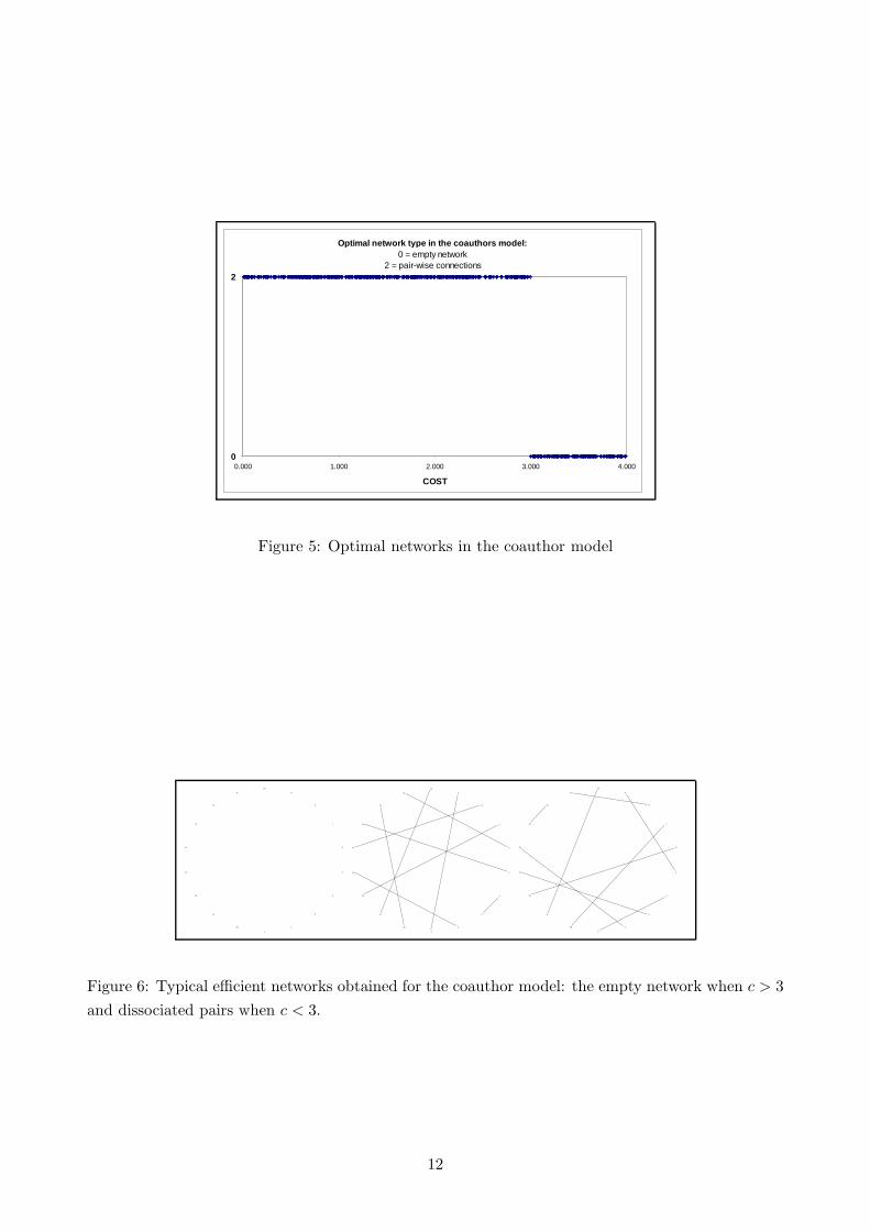
Optimal network type in the coauthors model: 0 = empty network
2 = pair-wise connections
0
2
0.000 1.000 2.000 3.000 4.000
COST
Figure 5: Optimal networks in the coauthor model
1
2
3
4
5
6
7
8
9
10
11
12
13
14
15
16
17
18
1
2
3
4
5
6
7
8
9
10
11
12
13
14
15
16
17
18
1
2
3
4
5
6
7
8
9
10
11
12
13
14
15
16
17
18
Figure 6: Typical efficient networks obtained for the coauthor model: the empty network when c > 3
and dissociated pairs when c < 3.
12

Table 2 provides the share of correct predictions of the GA for different values of n and for the
different optimal network structures (that should be predicted). The results are summarized in the
following propositions.
Proposition 5 In the connections model, both when g∅ or gN is the efficient structure, the GA
remarkably finds them whatever n (with 5 ≤ n < 20). It is only when g⋆ is the efficient network and
n increases that the GA might provide some incorrect estimations of the efficient networks.
For example, when n = 12, the GA is deceived in 3% of the cases corresponding to a star as the
optimal network.
Proposition 6 The probability that the GA provides a correct prediction of the connections model
globally decreases with the number of agents n, whereas it increases with the number of chromosomes
m and with the number of generations T .
Indeed, errors are partly due to an inefficient GA characterized by too few chromosomes or
too few generations. Nevertheless, we cannot establish a monotonic relationship between these two
dimensions of the GA and its effectiveness. We just empirically observe a region of best effectiveness
around 300 for the number of chromosomes and the number of generations. We hence use this value
in the next point that we explore.
Efficient network g⋆ g∅ gN
# of agents
5 1 1 1
6 1 1 1
7 1 1 1
8 1 1 1
9 0.98 1 1
10 1 1 1
11 1 1 1
12 0.97 1 1
13 0.87 1 1
14 0.97 1 1
15 0.87 1 1
16 0.76 1 1
17 0.67 1 1
18 0.76 1 1
19 0.71 1 1
Average 0.90 1 1
Table 2: Proportion of correctly predicted efficient networks depending on the number of agents and
the efficient network
In order to explore more in detail these deceiving cases, we run 500 simulation experiments
exclusively dedicated to the randomly drawn cases for which the star (g⋆) is the optimal network.
13

As explained above, the GA is used from this point on with m = T = 300. These experiments are
reported in Table 3. We observe therein that when n < 12, the GA offers only correct predictions.
When n ≥ 12 the GA is not always able to find the correct graph shape (g∗). The probability of
error, conditional to 20 > n ≥ 12, is 0.126. The non linearity of the network value state space leads
the GA to stabilize on local maxima. Nevertheless, even when deceived, the GA finds networks that
have an average social value equal to 98.66% the social value of g∗.
Share of good # of
# of agents predictions observations
5 1 25
6 1 29
7 1 31
8 1 31
9 1 30
10 1 36
11 1 32
12 0.94 35
13 0.93 27
14 0.95 39
15 0.90 41
16 0.82 33
17 0.69 39
18 0.92 37
19 0.86 35
Average 0.90 500
Table 3: Proportion of correctly predicted g∗ configurations with m = T = 300
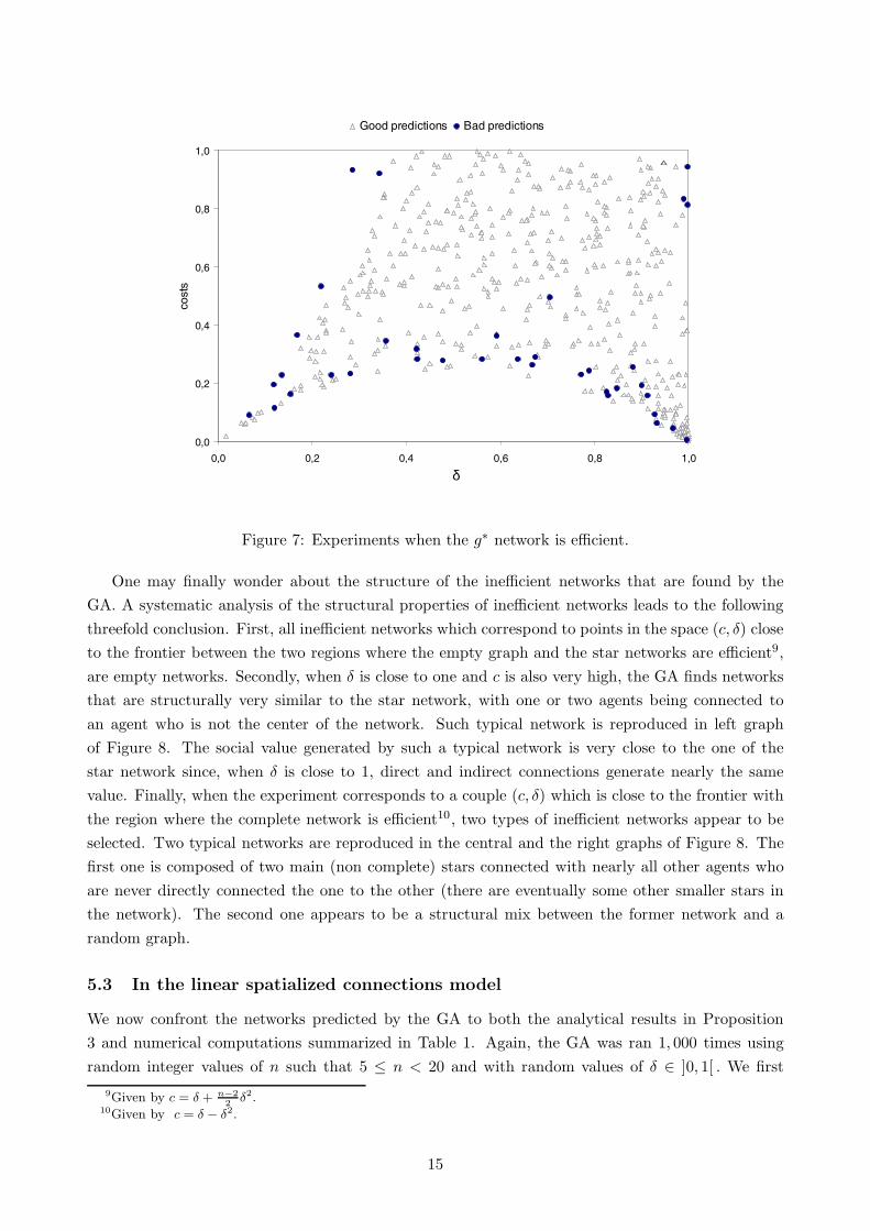
In order to better understand the nature of the deceptive configuration, we address the following
question: are mistaken predictions uniformly distributed over the state space (c, δ) for which stars
are optimal networks ? The Figure 7 represents all experiments performed for which the star is
the optimal network in the (c, δ) space, in accordance with the analytical predictions summed up
in Figure 1. The black dots on this figure represent the experiments for which the GA fails. If we
compare the position of these dots on the graph with the borders in Figure 7, it clearly appears
that the mistakes are not uniformly distributed, but located close to the borders (C1 and C2) of
the regions where optimal networks are different. Given that the crossover and mutation operators
explore the state-space in a discontinuous manner, they make the GA jump from one side of the
border to the other, making very difficult the finding of the optimal graph. Everywhere else, the GA
is efficient in finding the efficient star network.
Proposition 7 When g∗ is the optimal network of the connections model, the GA may fail to sys-
tematically find it when c and δ take values close from those that generate different optimal networks.
In these cases, the predicted networks still have an average social value equal to nearly 99% the social
value of g∗.
14
0,0
0,2
0,4
0,6
0,8
1,0
0,0 0,2 0,4 0,6 0,8 1,0
co
sts
Good predictions Bad predictions
δ
Figure 7: Experiments when the g∗ network is efficient.
One may finally wonder about the structure of the inefficient networks that are found by the
GA. A systematic analysis of the structural properties of inefficient networks leads to the following
threefold conclusion. First, all inefficient networks which correspond to points in the space (c, δ) close
to the frontier between the two regions where the empty graph and the star networks are efficient9,
are empty networks. Secondly, when δ is close to one and c is also very high, the GA finds networks
that are structurally very similar to the star network, with one or two agents being connected to
an agent who is not the center of the network. Such typical network is reproduced in left graph
of Figure 8. The social value generated by such a typical network is very close to the one of the
star network since, when δ is close to 1, direct and indirect connections generate nearly the same
value. Finally, when the experiment corresponds to a couple (c, δ) which is close to the frontier with
the region where the complete network is efficient10, two types of inefficient networks appear to be
selected. Two typical networks are reproduced in the central and the right graphs of Figure 8. The
first one is composed of two main (non complete) stars connected with nearly all other agents who
are never directly connected the one to the other (there are eventually some other smaller stars in
the network). The second one appears to be a structural mix between the former network and a
random graph.
5.3 In the linear spatialized connections model
We now confront the networks predicted by the GA to both the analytical results in Proposition
3 and numerical computations summarized in Table 1. Again, the GA was ran 1, 000 times using
random integer values of n such that 5 ≤ n < 20 and with random values of δ ∈ ]0, 1[ . We first
9Given by c = δ + n−22
δ2.10Given by c = δ − δ2.
15

1
2
3
4
5
6
7
8
9
10
11
12
13
14
15
16
1
2
3
4
5
6
7
8
9
10
11
12
13
14
15
16
1
2
3
4
5
6
7
8
9
1011
12
13
14
15
16
17
18
19
Figure 8: Some typical inefficient networks found by the GA at the internal frontiers of the region
where g∗ is the efficient network
find that the GA correctly founds all but one efficient networks among the runs that correspond to
configurations covered by Proposition 3 11.
Among the runs which are covered by the numerical computations of JG00 (when n = 5, 6 or 7;
185 runs), all their predictions are confirmed by the GA, with the following exceptions (see Figure 9):
• gC is not found by the GA, which instead selects gC′ = gC − 46 + 56. Simple computations
confirmed that indeed ∀δ ∈ ]0, 1[ , π(gC′
)> π
(gC
).
• gG is not found by the GA, which instead selects gG′ = gG − 13 + 14. Simple computations
confirm that π(gG′
)> π
(gG
)for all δ ∈ ]0.277, 0.936[ , a region which includes the one indicated
by JG00 as corresponding to gG as the efficient network (see Table 1).
• gD is not found by the GA, which instead selects gD′ = gD − 13 + 12. Simple computations
confirm that π(gD′
)> π
(gD
)when δ > 0.919, region in which our randomly drawn values of
δ are comprised. Of course, our results do not imply that gD is not the efficient network when
δ ∈ [0.8789, 0.919] .
• g2⋆ = 13, 23, 34, 35, 45, 56, 57 , a network constituted by two interlocked local stars (see Fig-
ure 9), is found for n = 7 and δ ∈ [0.835, 0.907] . In this region of δ, g2⋆ dominates g⋆⋆ and
gH , and it must be chosen even when the efficient network remains unspecified in JG00 (region
marked by an ?)12.
Proposition 8 In the linear spatialized connection model, the GA computations nearly always corre-
spond to the predictions of Proposition 3 and corroborate the predictions of JG00. When the networks
generated by the GA are different than the networks found by JG00, their social surplus is greater.
6 Efficient networks in the linear spatialized connections model
We now turn to the use of the GA technique to perform the first fully exploratory analysis of the
efficient networks in the linear spatialized connection model of JG00. The question we would like
11For instance, when n = 10, Proposition 3 yields that if δ < 0.10114, the empty network is the unique efficient
network, and if 0.10114 < δ < 0.11111, the chain network is the only efficient network.12g⋆⋆ is found as the most efficient network when δ ∈ [0.789, 0.810] , and gH is also efficient when δ ∈ [0.924, 0.969].
16

1 2 3 4 5 6
1 2 3 4 5 6
gC′ gD′
1 2 3 4 5 6 7
1 2 3 4 5 6 7
gG′ g2⋆
Figure 9: Original networks found by the GA as efficient for specific values of δ
to address here is related to the issue of the optimal creation of inter-individual connections and
their distribution among agents. Since the model exhibits positive externalities that deteriorate
geometrically with relational distance and bond costs that increase with linear exogenous distance,
we especially wonder to what extent the efficient networks need to be organized around central agents
or need to be locally connected. To put it differently, should the network be structured with one agent
in the middle who mediates the externalities between all others in a similar fashion as g⋆⋆ or even as
gG′? Should the network rather be locally coordinated with small stars in more peripheral positions
as in g2⋆? Should instead connections be only locally formed and thus more equally distributed
among agents? Should these various forms coexist in some extent? The answers to these questions of
course strongly depend on the decay parameter δ which determines the extent to which the network
is conducive to positive externalities.
We are willing to address these questions synthetically for different sizes of the population. There-
fore, we propose to rely on the following four simple indicators, to be computed for each GA efficient
network, that grasp most of the structural attributes we are interested in:
∆ (g) =1
n
∑i∈N
ηi (g)
(n− 1), (5)
Γ (g) =1
(n− 1)maxi∈N
ηi (g) , (6)
Ω (g) =1
(n− 1)second max
i∈Nηi (g) , (7)
Φ (g) =1
(n− 1)
∑ij∈g
l (i, j) . (8)
∆ (g) gives the average number of links per agent relative to the maximum number of links any
agent can sustain: (n − 1)13. Γ (g) gives the size of the largest neighborhood on network g again
scaled by the size of the largest possible neighborhood in a population of n agents. Ω (g) gives the
size of the second largest neighborhood on g, again scaled by (n− 1). Lastly, Φ (g) is the average
geographic distance in the network g, scaled by the maximum geographic distance when there are n
agents positioned in our linear world, that is the distance between the two agents located at the far
ends of the line: (n− 1). All indicators are positive and they can not exceed the unity.
13It is equal to twice the density of the network as it is usually refered to in the literature on social networks. This
density is equal to η (g) / (n (n − 1)) .
17

Let us now explain how the simultaneous analysis of the four indexes provides synthetical infor-
mation on the structuration of networks. A high value for Γ (g) and simultaneously a much lower
value for both Ω (g) and ∆ (g) indicate a structuration of the connections around a central agent. On
the contrary, if the network is not globally structured around one central agent, and if the two most
connected agents have a similar number of neighbors, then typically Γ (g) ≈ Ω (g). If, in addition
Ω (g) ≫ ∆ (g), then one can conclude that there are several (at least two) stars in the network.
Otherwise, if Ω (g) ≈ ∆ (g) , then agents are quite equal in the size of their neighborhoods. Lastly,
if Φ (g) is low, then it can be inferred that connections are mainly established in the geographical
neighborhoods.
0.2
.4
.6
.8
1
Me
dia
n b
an
ds
0 .2 .4 .6 .8 1
δ
Γ
Ω
∆
Φ
Figure 10: Median band values of Γ, Ω, ∆ and Φ computed for 1000 GA-efficient networks with
random integer values of n between 5 and 19 (inclusive) and with random values of δ ∈]0, 1[
We draw in Figure 10 the median bands of these indicators. Let us examine how do efficient
networks structures evolve with δ. When δ increases from 0 to 0.2, we observe that Γ (g) ≈ Ω (g) ≈
∆ (g) and, simultaneously, that Φ (g) remains low. That indicates that no star has been formed and
connections are mainly local. In this region, Φ (g) increases with δ because the density of efficient
networks increases: once connections at distance one are all formed then local density increases by
establishing connections at distance two and so on so forth. When δ increases from 0.2 up to 0.45,
Γ (g) increases up to unity which means that then one agent at least is connected to all others. In
the meantime, Ω (g) increases slowly to reach about 0.5. Both indexes remain on a plateau between
δ ≈ 0.45 and δ ≈ 0.65. In this region, one observes only a slight difference between Ω (g) and ∆ (g) .
In the meantime Φ (g) remains below 0.2 (in other words, the average geographic distance between
any two connected agents is on average equal to twenty percent of the distance between the far ends).
All this indicates that networks are mediated by a central agent who displays positive externalities in
the population. There are no significant secondary stars but a strong local density. It is only when
δ & 0.55 that the network density (grasped through ∆ (g)) begins to decrease. Simultaneously, Φ (g)
18

continues to increase. This indicates that the centrality of the star is reinforced because some local
connections have become inefficient and are not formed anymore. When δ ≈ 0.85, the density of
the central agent sharply decreases while the density of the second most connected agent decreases
less sharply. The need for global centralization is much reduced and a small window for more local
centralization appears (in a similar fashion as g2⋆).
Determinants of Γ
|delta< 0.2067
delta< 0.1318
n< 6.5
delta>=0.9474
delta< 0.3416
n< 11.5 n< 6.5
0.068n=121
0.036n=11
0.39n=61
0.51n=62
0.6n=63
0.81n=75
0.73n=75
0.94n=532
Determinants of Ω
|delta< 0.1675
delta< 0.09651
n< 7.5
delta>=0.757
n>=8.5 delta< 0.2201
n< 8.5 n>=7.5
delta< 0.3626
0.027n=86
0n=14
0.25n=56
0.38n=191
0.5n=62
0.26n=13
0.48n=34
0.54n=440
0.51n=23
0.65n=81
(a) (b)Determinants of Φ
|delta< 0.1715
delta< 0.08707
n< 7.5
n>=9.5
n>=14.5
delta< 0.2495
delta< 0.3038
delta>=0.9536
0.0081n=74
0n=16
0.092n=69
0.17n=293
0.15n=27
0.2n=246
0.17n=42
0.18n=16
0.25n=217
Determinants of ∆
|delta< 0.1675
delta< 0.08707
n< 7.5
delta>=0.8529
n>=7.5
delta>=0.9151
delta< 0.2476
delta>=0.7456
0.014n=74
0n=16
0.18n=66
0.18n=84
0.26n=55
0.35n=27
0.3n=76
0.36n=102
0.43n=500
(c) (d)
Figure 11: Distributions of ∆,Γ,Φ and Ω
In order to verify that our structural inferences based on the medians are fully consistent with
the raw data, we also rely on regression trees (Venables and Ripley [1999], chapter 10). A regression
tree establishes a hierarchy between independent variables using their contributions to the overall fit(R2
)of the regression for a given dependent variable. More exactly, it splits the set of observations
in sub-classes characterized by their value in terms of their contribution to the explained variance.
Regression trees are very flexible in the sense that they do not specify any functional relation between
the explained and the explaining variables. The tree gives a hierarchical sequence of conditions on the
19
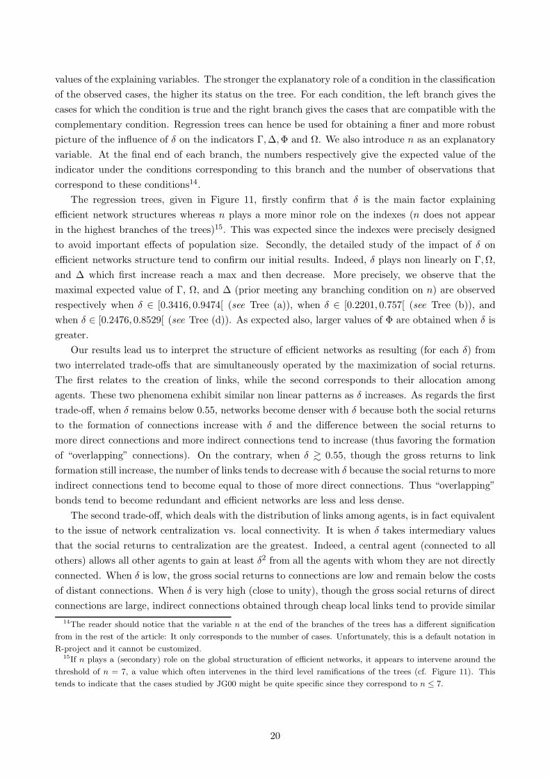
values of the explaining variables. The stronger the explanatory role of a condition in the classification
of the observed cases, the higher its status on the tree. For each condition, the left branch gives the
cases for which the condition is true and the right branch gives the cases that are compatible with the
complementary condition. Regression trees can hence be used for obtaining a finer and more robust
picture of the influence of δ on the indicators Γ,∆,Φ and Ω. We also introduce n as an explanatory
variable. At the final end of each branch, the numbers respectively give the expected value of the
indicator under the conditions corresponding to this branch and the number of observations that
correspond to these conditions14.
The regression trees, given in Figure 11, firstly confirm that δ is the main factor explaining
efficient network structures whereas n plays a more minor role on the indexes (n does not appear
in the highest branches of the trees)15. This was expected since the indexes were precisely designed
to avoid important effects of population size. Secondly, the detailed study of the impact of δ on
efficient networks structure tend to confirm our initial results. Indeed, δ plays non linearly on Γ,Ω,
and ∆ which first increase reach a max and then decrease. More precisely, we observe that the
maximal expected value of Γ, Ω, and ∆ (prior meeting any branching condition on n) are observed
respectively when δ ∈ [0.3416, 0.9474[ (see Tree (a)), when δ ∈ [0.2201, 0.757[ (see Tree (b)), and
when δ ∈ [0.2476, 0.8529[ (see Tree (d)). As expected also, larger values of Φ are obtained when δ is
greater.
Our results lead us to interpret the structure of efficient networks as resulting (for each δ) from
two interrelated trade-offs that are simultaneously operated by the maximization of social returns.
The first relates to the creation of links, while the second corresponds to their allocation among
agents. These two phenomena exhibit similar non linear patterns as δ increases. As regards the first
trade-off, when δ remains below 0.55, networks become denser with δ because both the social returns
to the formation of connections increase with δ and the difference between the social returns to
more direct connections and more indirect connections tend to increase (thus favoring the formation
of “overlapping” connections). On the contrary, when δ & 0.55, though the gross returns to link
formation still increase, the number of links tends to decrease with δ because the social returns to more
indirect connections tend to become equal to those of more direct connections. Thus “overlapping”
bonds tend to become redundant and efficient networks are less and less dense.
The second trade-off, which deals with the distribution of links among agents, is in fact equivalent
to the issue of network centralization vs. local connectivity. It is when δ takes intermediary values
that the social returns to centralization are the greatest. Indeed, a central agent (connected to all
others) allows all other agents to gain at least δ2 from all the agents with whom they are not directly
connected. When δ is low, the gross social returns to connections are low and remain below the costs
of distant connections. When δ is very high (close to unity), though the gross social returns of direct
connections are large, indirect connections obtained through cheap local links tend to provide similar
14The reader should notice that the variable n at the end of the branches of the trees has a different signification
from in the rest of the article: It only corresponds to the number of cases. Unfortunately, this is a default notation in
R-project and it cannot be customized.15If n plays a (secondary) role on the global structuration of efficient networks, it appears to intervene around the
threshold of n = 7, a value which often intervenes in the third level ramifications of the trees (cf. Figure 11). This
tends to indicate that the cases studied by JG00 might be quite specific since they correspond to n ≤ 7.
20

social returns because the spillovers do not much depend on social distance any more. Then, when
either δ is low or high, local connections of lower cost are preferably selected against costly distant
ones which are necessary to centralization.
The simultaneity of the two trade-offs makes that when efficient networks have a central agent
(when δ is intermediate), they are also much denser, especially in local areas. However, there is a
slight shift between the two trade-offs as δ varies, which produces specific network structures for
certain values of δ. When δ ≈ 0.2, the need for centralization is still not there while efficient networks
are already quite dense. Efficient networks are then strongly only locally connected. When δ ≈ 0.85,
efficient networks have a low connectivity while the need for centralization is still strong. This
configuration gives a small window for local stars to appear.
Proposition 9 In the linear spatialized connections model, when the decay of externalities is either
very low (δ close to 0) or very high (δ close to 1), networks should be only locally connected and no
central agent is needed. In intermediate cases, efficient networks are both centrally structured around
some coordinating agent and locally connected. On the borders between these three configurations, the
efficient networks are either only locally connected without any central coordination (when δ ≈ 0.2)
or coordinated by local stars (when δ ≈ 0.85).
7 Conclusions
One critical problem faced by economists interested in networks formation is the complete charac-
terization of the efficient networks for non trivial individual payoffs functions. We test in this paper
the relevance and the performances of an original method, namely the genetic algorithms (GA), for
computing such efficient network structures. In order to assess the efficacy of this technique, we com-
pute GA-efficient networks in models for which benchmark results are available. Our results show
that the GA are a powerful tool for network optimization. More precisely, in the coauthor model of
JW96, the GA is able to find the optimal structures in all simulations. In the connections model
of JW96, the GA finds again the efficient network structures but it can be deceived on the borders
between the areas corresponding to two distinct optimal structure (between empty network and the
star, as well as between the complete network and the star). In the interior of these areas, the GA
perfectly determines the relevant optimal network structure. In the linear spatialized connections
model of JG00, the GA performs almost perfectly when analytical results are available and are more
efficient than the numerical techniques employed by JG00 for a limited number of agents.
Then, an explorative use of the GA for computing efficient networks in the linear spatialized con-
nections model allows us to discuss the issue of the efficient structuration of networks. We find that,
depending on the parameter tuning the decay of positive externalities through connections, networks
should be structured quite differently. When the decay is either very low or very high, networks
should be only locally connected and no central agent is needed. When externalities are low, the so-
cial returns to distant connections can not compensate their high costs. When externalities are very
high, centralization becomes not socially desirable anymore since social distance becomes ineffective
on externalities. In between, networks should be both centrally structured around some coordinating
agent and locally connected. Therefore, centralization and local structuration are mostly found to
be complementary rather than exclusive. Nevertheless, it should be noticed that efficient networks
21

have very different shape when δ shifts from 0.2 to 0.4. Indeed, they shift from local connectivity
with all agents having the same number of connections and without any central coordination, to the
emergence of a star agent connected to all others while the connectivity of the others remain nearly
constant.
The GA technique may be further employed for exploring the optimal network structures in other
models for which analytical or even computational results on efficient structures can not be provided.
Another obvious application is to systematically compare the structural properties of the emergent
and of the efficient networks (for an exploration see Carayol, Roux and Yıldızoglu, 2007).
References
Carayol, N. and Roux, P. (2006) Knowledge flows and the geography of networks. The strategic
formation of small worlds, Working Paper BETA #2006-16, Universite Louis Pasteur, Strasbourg,
France.
Carayol, N. and P. Roux (2004) Behavioral foundations and equilibrium notions for social network
formation processes, Advances in Complex Systems, 7(1), 77-92.
Carayol, N. Roux, P. and M. Yıldızoglu (2006) Inefficiencies in a model of spatial networks formation
with positive externalities, forthcoming in Journal of Economic Behavior and Organization.
Dawid, H. (1999) Adaptive Learning by Genetic Algorithms, Springer, Berlin.
Debreu, G. (1969) Neighboring economic agents, La Decision, 171:85-90.
Goldberg, D. (1991) Genetic Algorithms, Addison Wesley, Reading:MA.
Holland, J. H. (2001) Adaptation in Natural and Artificial Systems, MIT Press, Cambridge:MA, sixth
printing.
Jackson, M.O. (2004) A Survey of Models of Network Formation: Stability and Efficiency, Chapter 1 in
Demange G. and M. Wooders (eds), Group Formation in Economics: Networks, Clubs and Coalitions,
Cambridge University Press, Cambridge U.K.
Jackson, M.O. and A. Wolinski (1996) A strategic model of social and economic networks, Journal of
Economic Theory, 71, 44-74.
Johnson, C. and R.P. Gilles (2000) Spatial social networks, Review of Economic Design, 5, 273-299.
Michalewicz, Z. (1996) Genetic Algorithms + Data Structures = Evolution Programs, Springer-Verlag,
Berlin.
Mitchell, M. (1996) An Introduction to Genetic Algorithms, MIT Press, Cambridge:MA.
Vallee, T. and M. Yıldızoglu (2004) Presentation des algorithmes genetiques et de leurs applications
en economie, Revue d’Economie Politique, 114(6), 711-745.
Venables, W. & Ripley, B. (1999) Modern Applied Statistics with S-PLUS, Springer.
Yıldızoglu, M. (2002) Competing R&D Strategies in an Evolutionary Industry Model, Computational
Economics, 19, 52-65.
22

Cahiers du GREThA Working papers of GREThA
GREThA UMR CNRS 5113
Université Montesquieu Bordeaux IV Avenue Léon Duguit
33608 PESSAC - FRANCE Tel : +33 (0)5.56.84.25.75 Fax : +33 (0)5.56.84.86.47
www.gretha.fr
Cahiers du GREThA (derniers numéros)
2007-01 : GONDARD-DELCROIX Claire, Entre faiblesse d’opportunités et persistance de la pauvreté : la pluriactivité en milieu rural malgache
2007-02 : NICET-CHENAF Dalila, ROUGIER Eric, Attractivité comparée des territoires marocains et tunisiens au regard des IDE
2007-03 : FRIGANT Vincent, Vers une régionalisation de la politique industrielle : l’exemple de l’industrie aérospatiale en Aquitaine
2007-04 : MEUNIE André, POUYANNE Guillaume, Existe-t-il une courbe environnementale de kuznets urbaine ? Emissions polluantes dues aux déplacements dans 37 villes
2007-05 : TALBOT Damien, EADS, une transition inachevée. Une lecture par les catégories de la proximité
2007-06 : ALAYA Marouane, NICET-CHENA Dalila, ROUGIER Eric, Politique d’attractivité des IDE et dynamique de croissance et de convergence dans les Pays du Sud Est de la Méditerranée
2007-07 : VALLÉE Thomas, YILDIZOĞLU Murat, Convergence in Finite Cournot Oligopoly with Social and Individual Learning
2007-08 : CLEMENT Matthieu, La relation entre les transferts privés et le revenu des ménages au regard des hypothèses d’altruisme, d’échange et de partage des risques
2007-09 : BONIN Hubert, French banks in Hong Kong (1860s-1950s): Challengers to British banks?
2007-10 : FERRARI Sylvie, MERY Jacques Equité intergénérationnelle et préoccupations environnementales. Réflexions autour de l'actualisation
2007-11 : CARAYOL Nicolas, ROUX Pascale, YILDIZOGLU Murat, In search of efficient network structures: The needle in the haystack
La coordination scientifique des Cahiers du GREThA est assurée par Sylvie FERRARI et Vincent
FRIGANT. La mise en page est assurée par Dominique REBOLLO.