Embed Size (px)
Citation preview

Reproduced with permission of the copyright owner. Further reproduction prohibited without permission.
ÉCOLE DE TECHNOLOGIE SUPÉRIEURE UNIVERSITÉ DU QUÉBEC
THESIS PRESENTED TO ÉCOLE DE TECHNOLOGIE SUPÉRIEURE
SUBMITIED li~ PARTIAL FULFILLMENT OF THE REQUIREMENTS FOR THE DEGREE OF
DOCTOR OF PHILOSOPHY
BY SIXTO ERNESTO GARCIA AGUILAR
OPTIMIZATION OF FLIGHT CONTROL PARAMETERS OF AN AIRCRAFT USING GENETIC ALGORITHMS
MONTREAL, NOVEMBER 18th, 2005
© Copyright by Sixto Ernesto Garcia Aguilar

Reproduced with permission of the copyright owner. Further reproduction prohibited without permission.
THIS DISSERTATION HAS BEEN EVALUATED
BY A COMMITTEE COMPOSED OF:
M. Maarouf Saad, superviser Electrical Department of École de technologie supérieure
Mme. Ouassima Akhrif, co-superviser Electrical Department of École de technologie supérieure
M. Mohamed Cheri et, president of jury Automatic Production Department of École de technologie supérieure
M. Jean de Lafontaine, jury Electrical Engineering Department of University of Sherbrooke
M. Jean Bertos Simo, external jury
IT HAS BEEN PRESENTED AS PART OF A PUBLIC DEFENSE
OCTOBER 12TH 2005
AT ÉCOLE DE TECHNOLOGIE SUPÉRIEURE

Reproduced with permission of the copyright owner. Further reproduction prohibited without permission.
To my daughters Marfa-Gabriela and Anita, to my wife
Anjela, and to my parents Victor and Gladys.

Reproduced with permission of the copyright owner. Further reproduction prohibited without permission.
OPTIMIZATION OF FLIGHT CONTROL PARAMETERS OF AN AIRCRAFT USING GENETIC ALGORITHMS
Sixto Ernesto Garcfa Aguilar
ABSTRACT
Genetic Algorithms (GAs) are stochastic search techniques that mimic evolutionary processes in nature such as natural selection and natural genetics. They have shown to be very useful for applications in optimization, engineering and learning, among other fields. In control engineering, GAs have been applied mainly in problems involving functions difficult to characterize mathematically or known to present difficulties to more conventional numerical optimizers, as weil as problems involving non-numeric and mixed-type variables. In addition, they exhibit a large degree of parallelism, making it possible to effectively exploit the computing power made available through parallel processing.
Despite active research for more than three decades, and success in solving difficult problems, GAs are still not considered as an essential global optimization method for sorne practical engineering problems. While testing GAs by using mathematical functions has a great theoretical value, especially to understand GAs behavior, these tests do not operate under the same factors as reallife problems do. Among th ose factors it is worth to mention two possible situations or scenarios: one is when a problem must be solved quickly on not too many instances and there are not enough resources (time, money, and/or knowledge); and the other is when the objective function is not "known" and one can only "sample" it. The first scenario is realistic in engineering design problems where GAs must have a relatively short execution time in achieving a global optimum and a high enough effectiveness (closeness to the true global optimum) to avoid several iterations of the algorithm. The second scenario is also true in the design of technical systems that generally require extensive simulations and where input-output behavior cannat be explicitly computed, in which case sampling becomes necessary.
F1ight control design presents these two types of scenarios and, during the last ten years, such problems as structure-specified H 00 controllers design, dynamic output feedback with eigenstructure assignment, gain scheduled controllers design, command augmentation system design, and other applications have been targeted using genetic methods. Although this research produced very interesting results, none so far has focused on reducing the execution time and increasing the effectiveness of GAs.
The efficiency and effectiveness of Genetic Algorithms are highly determined by the degree of exploitation and exploration throughout the execution. Several strategies have been developed for controlling the exploitation/exploration relationship for avoiding the

Reproduced with permission of the copyright owner. Further reproduction prohibited without permission.
11
premature convergence problem. While significant body of expertise and knowledge have been produced through severa! years of empirical studies, no research has reported the use of Bayes Network (BN) for adapting the control parameters of GAs in order to induce a suitable exploitation/exploration value.
The present dissertation fiiis the gap by proposing a model based on Bayes Network for controiiing the adaptation of the probability of crossover and the probability of mutation of a Real-Coded GA. The advantage of BNs is that knowledge, Iike summaries of factual or empirical information, obtained from an expert or even by Iearning, are interpreted as conditional probability expressions. It is important to highlight that our interest, which is motivated by the requirements of real applications, is the behavior of GAs within reasonable time bound and not the Iimit behavior. Related genetic algorithm issues, such as the ability to main tain diverse solutions along the optimization process, are also considered in conjunction with new mutation and selection operators.
The application of the new approach to eight different realistic cases along the flight control envelope of a commercial aircraft, and to severa! mathematical test functions demonstrates the effectiveness of GAs in solving f!ight-control design problems in a single run.

Reproduced with permission of the copyright owner. Further reproduction prohibited without permission.
L'OPTIMISATION DES PARAMÈTRES DE CONTRÔLE D'UN AVION EN UTILISANT DES ALGORITMES GÉNÉTIQUES
Sixto Ernesto Garda Aguilar
SOMMAIRE
Problématique
La conception d'un avion commercial est non seulement un processus complexe mais également très long, qui exige l'intégration de plusieurs technologies. Les ingénieurs doivent formuler des solutions optimales pour développer des produits satisfaisant de rigoureuses caractéristiques. Ils portent une responsabilité lourde car leurs idées, leurs connaissance et leurs habilités ont des impacts significatifs sur la performance de l'avion, comme son coût et son entretien, ainsi que son opération rapide et robuste.
Parmi les différentes phases du processus de conception, l'une des plus importantes est celle où les ingénieurs de conception d'avion doivent fournir la structure du système de commande électrique de vol-par-fil (fly-by-wire). Contrairement aux systèmes conventionnels de commande de vol où le pilote déplace l'avion en utilisant des mécanismes mécaniques ou hydromécaniques, le vol électrique comporte des entrées électriques et électroniques de la cabine de pilotage vers les gouvernes. En utilisant un système de comande de vol électrique, les ordres des pilotes sont augmentés par des entrées additionnelles à partir des ordinateurs de commande de vol, lui permettant de pousser l'avion aux limites de 1' enveloppe de vol et recevoir une réponse commandée et sécuritaire. En d'autres termes, un système de vol électrique est construit pour interpréter l'intention du pilote et pour la traduire en action, où le processus de traduction prendra en considération des facteurs de l'entourage. Ceci prévoit une commande plus sensible et plus précise de l'avion, qui permet une conception aérodynamique plus efficace ayant pour résultat la drague réduite, la brûlure améliorée de carburant et charge de travail réduite pour le pilote.
La plupart des circuits de commande de vol se composent des déclencheurs, de dispositifs de senseurs ainsi que des gains des contrôleurs. Les valeurs pour l'ensemble des gains du contrôleur doivent être choisit afin d'assurer la performance optimale de l'avion sur toute l'enveloppe de vol, s'accordant aux conditions définies par des organismes de gouvernement comme l'Administration fédérale d'aviation des Etats-Unis et l'Autorité d'aviation civile du Royaume Uni. D'une façon générale. le design industriel d'un circuit de commande de vol inclut les activités suivantes: a) dériver les composantes d'un modèle dynamique non linéaire pour l'avion; et b) analyser la structure hypothétique du modèle et de son comportement dynamique en employant la simulation non linéaire. La dernière activité non seulement inclut l'exécution du modèle de simulation pour plusieurs points

Reproduced with permission of the copyright owner. Further reproduction prohibited without permission.
IV
des opérations de 1' enveloppe de vol, mais également des tâches d'optimisation pour trouver des valeurs optimales pour les gains de contrôleur pour chaque point d'opération. Les points d'opération de l'enveloppe de vol sont des conditions de vol appropriées selon la vitesse, centre de gravité, poids, pression et altitude qui sont capturées à partir de vraies situations pour être utilisées dans le modèle de simulation.
Le type de méthodes d'optimisation et l'exactitude de l'optimisation des modèles utilisés sont très critiques pour rendre plus efficace et efficiente la tâche de trouver un ensemble optimal de gains de contrôleur. Tandis que les techniques basées sur le calcul sont locales dans leur portée et dépendent de l'existence de l'une ou l'autre des dérivées ou un certain arrangement d'évaluation de fonctions, les algorithmes énumératifs de recherche manquent d'efficacité quand augmente la dimensionnalité du problème. Les concepteurs que utilisent des méthodes d'optimisation classiques choisissent normalement un premier point de départ pour 1' algorithme. Si ce premier point est assez proche de la solution optimale, alors la technique convergera vers elle. Dans le cas contraire, le point initial doit être modifié selon une stratégie utilisée par le concepteur. Ainsi, trouver une bonne solution est très itérative et compte sur l'expérience du concepteur avec le processus d'optimisation, ce qui rapporte rarement un optimum global. Par conséquent, il est nécessaire de chercher un algorithme d'optimisation robuste et global pour résoudre le problème et pour améliorer le processus de conception.
Cadre Conceptuel
Nous avons choisi les algorithmes génétiques (GAs) pour résoudre ce problème. Les GAs ont subi un grand développement au cours des dernières années, ont été reconnus comme une méthode fiable d'optimisation, et ont montré une efficacité remarquable en résolvant des problèmes non linéaires avec des nombres élevés de variables. On les classe comme un sous-ensemble d'un groupe de procédures heuristiques connues sous le nom de méthodes de Calcul Évolutionnaire (EC) qui inclut également les Stratégies d'Évolution (ES), la Programmation Génétiques (PG) et la Programmation Évo1utionnaire (PE). Les méthodes de calcul évolutionnaire sont des algorithmes stochastiques dont ses méthodes de recherche modélisent deux importants phénomènes de la nature : transmission génétique et le principe de Darwin pour la survie.
Plusieurs conditions rendent les GAs appropriés pour trouver les gains optimaux du contrôleur d'un modèle non linéaire, comme celui utilisé pour la conception d'un système de commande de vol d'un avion jet d'affaires. Parmi ces conditions, nous avons que: 1) la fonction de coût n'a pas besoin d'être une fonction explicite; elle est possible d'être définie à partir d'une des sorties d'un modèle de simulation; 2) nous n'avons pas besoin de conditions initiales; 3) on peut trouver une solution globale optimale ou très proche de celle-ci, même si la fonction de coût est fortement non linéaire, multi variable et multimodale.

Reproduced with permission of the copyright owner. Further reproduction prohibited without permission.
v
Afin d'exécuter efficacement la recherche d'un optimum sur les espaces de solutions pauvrement définis, les GAs classique utilisent la technique des chromosomes de Bolland. Il s'agit d'une méthode de codification de l'espace de solution utilisant de brèves chaînes de caractères binaires, 1 et 0, agencés de manière à former un chromosome unique. Cependant, il est possible d'utiliser aussi de chaînes de caractères réels comme dans le cas des algorithmes génétiques de codage réel (RGAs). Chaque chaîne représente (ou en quelque sorte permet d'étiqueter) une solution potentielle du problème d'optimisation, solution qui est préalablement évaluée en rapport à la fonction objective à optimiser. Afin d'identifier d'autres solutions à évaluer, de nouvelles chaînes de caractères sont produites après l'application des opérateurs génétiques, soit la recombinaison et la mutation, à celles existantes. Ces opérateurs, lorsque combinés à un processus de sélection naturelle, permettent l'utilisation efficace d'information d'hyperplan du problème pour guider la recherche. Chaque fois qu'une nouvelle chaîne est produite, les GAs font l'échantillonnage de l'espace de solutions possibles. Après une série de prélèvements guidés, l'algorithme devient centré de plus en plus dans les points près de la solution globale supposée.
Le succès de ces algorithmes est fondé sur l'équilibre entre l'exploitation des meilleures chaînes trouvées et l'exploration du reste de l'espace de recherche. L'un des buts les plus importants à ce stade est de ne pas rejeter de bonnes régions où un véritable optimal global peut exister. Cependant, les GAs comptent sur beaucoup de paramètres, et 1' utilisation des arrangements faibles peuvent empêcher d'atteindre un équilibre correct entre l'exploitation et 1' exploration. Ceci peut dégrader sévèrement la performance du GA en provoquant une possible convergence prématurée, et ainsi forcer le concepteur à faire exécuter le GA plusieurs fois. De plus, la conception de systèmes techniques, telles que les systèmes de vol électrique pour les avions d'affaires, exigent des simulations étendues où le comportement d'entrée-sortie du système ne peut pas être explicitement calculé, et où le prélèvement est nécessaire. Contraire à l'optimisation des fonctions mathématiques utilisant les GAs, où le temps d'évaluation de la fonction objective est juste une fraction de millisecondes, la simulation des problèmes réels peut exiger de 1' ordinateur beaucoup de temps d'exécution juste pour évaluer la fonction objective.
Par conséquent. le but à accomplir dans cette recherche est d'améliorer la performance des algorithmes génétiques afin de les rendre plus efficients et efficaces pour l'optimisation des gains du contrôleur d'un système de vol électrique des avions commerciaux. Par efficacité, nous voulons dire que quelque soit la solution produite par notre GA amélioré, nous devrions tomber très près du vrai optimum global (petit écart type) indépendamment de combien de fois le GA est invoqué. Quant à l'efficience, nous voulons dire que notre GA amélioré devrait résoudre le problème dans le moindre de temps (petit temps de CPU) que le GA classique, sans affecter son efficacité.

Reproduced with permission of the copyright owner. Further reproduction prohibited without permission.
vi
Méthodologie
La méthodologie appliquée dans cette recherche a pennis l'étude de différentes architectures de GA pour arriver à une configuration de base, celle qui a été modifiée par chacune de nos contributions. Il est important de souligner que la flexibilité est essentielle dans la conception des GAs, et seulement dans quelques occasions les résultats assortissent des hypothèses préconçues. Plusieurs GAs améliorés sont fréquemment cités dans la littérature, avec la motivation d'être une nouveauté. Cependant, dans plusieurs cas, les GAs précédemment présentés sont plus simples et ont une exécution identique ou meilleure.
La recherche dans le domaine des GAs a été dominée par deux types opposés d'approches, soit l'expérimentation ad-hoc et la recherche d'un modèle exact pour le GA. Trouver un modèle exact pour les GAs est devenu une tâche plus complexe et plus difficile analytiquement que les GAs eux-mêmes, et seulement dans très peu d'occasions a-t-on pu développer des conceptions améliorées pour les GAs. La difficulté réside dans le fait que ce sont des systèmes complexes, et donc par conséquent indétenninés. Une meilleure approche est de combiner l'intuition et l'expérience quant au système à résoudre, l'analyse globale et comparative des résultats, et l'expérimentation systématique de diverses architectures.
Cette méthodologie nous a pennis de répondre à six questions reliées à l'analyse, la conception et le test de notre GA, soit : 1) quel langage de programmation nous devrions utiliser; 2) si nous devrions utiliser des logiciels pours les GAs déjà conçus, ou plutôt le faire par nous même; 3) dans quelle partie de l'architecture du GA nous devrions concentrer nos efforts pour faire des nouvelles contributions théoriques et empiriques ; 4) quels types de tests nous devrions appliquer à nos nouvelles conceptions et pour comparer les résultats avec d'autres travaux de recherche dans la littérature; 5) quel type d'index peut nous permettre d'évaluer la perfonnance de nos GAs; et 6) quels cas de l'enveloppe de vol de 1' avion à 1 'étude nous devrions utiliser pour tester nos GAs.
Trois principes fondamentaux nous on guidé durant cette recherche pour en assurer la qualité. Premièrement, il fallait que toute amélioration au GA reste simple en tennes de conception et d'exécution. Il est déjà difficile d'analyser un système aussi complexe qu'un algorithme génétique, il serait donc peu valable d'augmenter le coût de la complexité du système pour ne mener qu'à de faibles améliorations. En second lieu, il nous importait d'effectuer une solide analyse du système, et ce par une application intelligente des heuristiques, de la connaissance et de l'expertise que nous avons obtenues des concepteurs du système. Troisièmement, nous avons tenu à mener une expérimentation détaillée et soigneuse pour examiner plusieurs nouvelles méthodes, plutôt que de nous fier simplement aux méthodes antérieures de résolution des GAs.
Les spécifications du système à résoudre, les données de base sur les enveloppes de vol,

Reproduced with permission of the copyright owner. Further reproduction prohibited without permission.
V li
ainsi que les ressources pour soutenir cette étude ont été fournies par Bombardier.
Contributions
Afin de viser la première partie de nos objectifs, soit 1' efficience du processus de recherche de solution, un nouvel opérateur de mutation a été mis en application. Nous avons réussi à combiner les caractéristiques de deux opérateurs de mutation, uniforme et non uniforme, au sein d'un nouvel opérateur de type périodique. Ce nouvel opérateur nos a permis d'obtenir des contrôleurs qui produisent le plus petit coût minimal pour les huit cas du système à l'étude, avec des moyennes et écarts types plus petits et plus stables que ceux obtenus avec les opérateurs uniformes et non uniformes en utilisant un maximum de deux cents générations. Cependant, l'utilisation d'une technique déterministe pour le contrôle de paramètres dans la conception de l'opérateur périodique de mutation ne nous a pas sauvé du processus de 1' accord manuel, mais il a amélioré l'efficacité de notre GA dans le problème de conception de la loi de commande d'avion.
Quant à l'efficacité à résoudre un problème réel d'optimisation, nous avons pris en compte qu'elle dépend de l'exactitude du modèle employé pour mettre en application la fonction objective. Tandis que le modèle sans contrainte fourni par Bombardier inclut les critères de qualité de manipulation qui doivent être satisfaits selon des conditions des régulateurs, il n'y a pas de manière directe de contrôler la forme de sa réponse à l'échelon. Ainsi, nous avons proposé un nouveau modèle avec contraintes et nous avons fait la conception d'un nouvel opérateur de sélection detournement stochastique pour augmenter l'efficacité d'un algorithme génétique du codage réel (RGA) appliqué aux problèmes d'optimisation avec contraintes. Pour la conception de 1 'opérateur de sélection de tournement stochastique contraint, on a appliqué une méthode qui peut manipuler la proportion d'individus faisables et non faisables sans négliger le comportement dynamique du GA. Les gains des contrôleurs obtenus avec le nouveau modèle et le nouvel opérateur ont été capables de produire de meilleures réponses à l'échelon que le modèle sans contraintes en satisfaisant en même temps les critères de qualité de manipulation du système. De plus, les moyennes et les écarts types obtenus ont été plus stables et dans quelques cas plus petits que ceux produits par des autres méthodes évolutives. Ce nouveau modèle contribue au concepteur avec une manière flexible de contrôler les caractéristiques de la réponse du système.
Bien que le temps de calcul ne soit pas significatif dans le cas d'une optimisation des fonctions numériques, il est très important quand nous employions la simulation des problèmes réels dans plusieurs domaines parce que ceci a pu impliquer beaucoup de temps d'exécution juste pour évaluer la fonction objective. Ainsi, il est donc crucial de savoir quand arrêter le processus d'optimisation d'un GA ou détecter quand le processus d'optimisation exécuté par un GA est plus utile.
En combinant notre modèle avec l'utilisation d'un index pour mesurer la diversité des in-

Reproduced with permission of the copyright owner. Further reproduction prohibited without permission.
Vlll
dividus d'une population d'un algorithme génétique ainsi qu'un réseau de Bayes (BN), nous avons réussi à inclure notre connaissance et expertise partielles du système afin de détecter la convergence et pour arrêter le processus d'optimisation. L'applicadon d'un index, comme l'index de la diversité modifié de Simpson (mD), qui est souvent employé pour mesurer la biodiversité d'un habitat en écologie a permis de mesurer la dissimilitude des gènes dans une population pendant le processus d'optimisation d'un algorithme génétique de codage réel (RGA) qui emploient des opérateurs de mutation avec des politiques décroissantes de mutation.
Il nous fut également nécessaire de créer un nouveau processus pour l'application de cet index dans le contexte des RGAs. Ce processus a prouvé l'existence d'un ensemble de classes des chromosomes autour du meilleur individu avec certaines caractéristiques où leur diversité devient critique pour détecter la convergence. Les résultats ont démontré que quand l'index modifié de Simpson était au-dessous d'une certaine valeur KmD puis la probabilité que la convergence s'est produite était très haute. Le réseau de Bayes, nous a permis de matérialiser une nouvelle méthode de détection de convergence et un nouvel algorithme génétique adaptatif probabiliste en utilisant l'information obtenue à partir du nouveau processus et de notre propre expertise. Les résultats démontrent clairement que nous avons réussi à diminuer de 25% le temps d'exécution original et à améliorer l'efficacité des RGAs. Tandis que nous considérions que l'adaptation de l'opérateur de mutation non uniforme n'est pas meilleure que nous puissions faire en utilisant mD et nos BN, cet opérateur nous montre sans difficulté la manière d'améliorer l'opérateur de mutation existant.
Recherches Futures
Cependant, plus de travail reste à faire et nous suggérons un certain nombre de suites potentielles du travail décrit dans cette thèse.
Entre autres, il sera très important de savoir si l'index modifié de Simpson peut être appliqué à différentes architectures de RGAs. Par différentes architectures, nous avons l'intention de nous référer à différents types d'opérateur de croisement et de mutation.
Un autre travail qui reste à effectuer est de voir si l'index employant un ensemble différent de classes peut laisser savoir avec plus de précision le comportement du RGA à différentes étapes autres que la dernière.
Il serait aussi très intéressant et utile de trouver un modèle mathématique qui relie la variable epsilon avec la précision des résultats finaux. De cette façon on pourrait peut-être savoir et commander la précision de n'importe quelle solution du RGA.
En suivant les directives de la méthodologie utilisée dans cette recherche, il est important

Reproduced with permission of the copyright owner. Further reproduction prohibited without permission.
ix
de voir la possibilité de faire une extension de l'utilisation de l'index modifié de Simpson et le réseau de Bayes pour contrôler le comportement dynamique de 1' opérateur de croisement.
Une autre prolongation de cette recherche devrait être l'utilisation du réseau de Bayes et un index de diversité semblable à celui employé dans cette recherche, pour améliorer l'exécution du RGA cherchant à résoudre des problèmes d'optimisation avec contraintes. Un bon candidat pourrait être le rapport des individus faisables et non faisables de chaque génération dans toute la duré du processus d'optimisation.
Enfin, bien que cette recherche a montré l'utilisation du réseau de Bayes et un index de diversité à RGA, il reste explorer leur utilisation dans des GAs où le codage est différent, tel que binaire et nombre entier.

Reproduced with permission of the copyright owner. Further reproduction prohibited without permission.
ACKNOWLEDGEMENTS
First and foremost, I would like to sincerely thank my supervisors, Professors Maarouf
Saad and Ouassima Akhrif. Dr. Saad did not only introduce me to the Evolutionary Com
putation world but also provided me with a free exchange of ideas, constructive criticism,
encouragement, ad vice and financial and moral support during the course of my graduate
studies at ETS. I express my sincere gratitude to him for the confidence that he granted me
especially when I proposed to apply Bayes Network to GA. Dr. Ouassima Akhrif granted
me three years of fi.nancial support through the Bombardier project. Her assessments and
valuable criticism of my work, as weil as her advices helped me bring this thesis to its
natural conclusion.
I wish to thank Professors Mohamed Cheriet, Jean de Lafontaine and Dr. Jean Bertos
Simo for serving on my PhD. committee and for providing many useful comments and
suggestions.
I address my thanks to all the members in Bombardier research group for their assistance,
their support and for providing a congenial environment for me to work in.
Thank y ou to the who le staff of the Library of ETS.
Dr. Stephane Gagnon deserves a special mention for his friendship and for many enlight
ening discussions. He was a good source of motivation - sometimes he seemed more
excited about my work than I was.

Reproduced with permission of the copyright owner. Further reproduction prohibited without permission.
xi
Thanks very much, Frank Scarpelli, for your friendship, generosity, concern and warmth
to me and my family.
1 thank my Parents for their love and support from my first day of life; my brothers and
sister for encouragement. To my relatives and friends who gave me their moral support
during ali these long years.
To Anjela Rousiouk, Anita and Maria-Gabriela, my lovely wife and daughters, for helping
me enjoy myself and take my mind off things when not working. Their love and support
were one of my main sources of strength in sorne of the crucial moments during the writing
of this thesis.
Thanks also go to ETS and Bombardier Aerospace lnc. for the funding without which 1
would not have been able to undertake this work. I also wish to acknow led ge FUNDACYT
(Fundacion para la Ciencia y la Tecnologia) and ESPOL (Escuela Superior Politecnica
del Litoral) for giving me the financial support and the opportunity to study my PhD in
Canada.

Reproduced with permission of the copyright owner. Further reproduction prohibited without permission.
TABLE OF CONTENTS
ABSTRACT.
SOMMAIRE
ACKNOWLEDGEMENTS.
TABLE OF CONTENTS
LIST OF TABLES .
LIST OF FIGURES .
CHAPTER 1 INTRODUCTION
1.1 1.2 1.3 1.4
CHAPTER2
2.1 2.1.1 2.1.2 2.1.3 2.1.3.1 2.1.3.2 2.1.3.3 2.1.3.4 2.1.3.5 2.1.4 2.1.5 2.1.6 2.1.6.1 2.1.6.2 2.1.6.3 2.1.6.4 2.1.6.5 2.2 2.2.1 2.2.1.1 2.2.1.2 2.2.1.3
Motivation . . . . . Research Objectives Contributions . . . . Outline of the Thesis .
BACKGROUND ON GENETIC ALGORITHMS
Simple Genetic Algorithm . . . . . . . . . . Encoding mechanism . . . . . . . . . . . . Strategy for generating the initial population Crossover Operator . . Single-point crossover . Two-point crossover . Multi-point crossover . Uniform crossover ... Positional and distributional biases Mutation .... Fitness function . . . . . . . . . . Selection ............. . Proportional Selection (or Roulette Wheel) Ranking Method . . . . . . Geometrie Ranking Method Tournament selection . . . Truncation selection . . . . Real-Valued Genetic Algorithms . Crossover operator . . . . . . Discrete recombination (DR) Blend Crossover (BLX- a) Linear recombination (LR) .
Page
111
x
xii
xv
xvii
1 4 4 5
8
10 10 12 13 13 14 15 15 16 17 18 18 20 21 22 Î"' _.)
Î"' _.)
Î"' _.)
24 25 25 26

Reproduced with permission of the copyright owner. Further reproduction prohibited without permission.
2.2.1.4 2.2.1.5 2.2.2 2.2.2.1 2.2.2.2 ???"' -·-·-·.)
2.2.2.4 ??"' -·-·.) 2.3 2.4
CHAPTER3
3.1 "'? .)._
3.2.1 "'?? .). __ _ "'?"' .).-. .)
3.2.4 3.3 3.3.1
CHAPTER4
4.1 4.2 4.3
CHAPTER5
5.1 5.2 5.2.1 5.2.2 5.2.3 5.3 5.3.1 5.3.2
CHAPTER6
6.1 6.2 6.3 6.4 6.4.1
Fuzzy recombination (FR) . SBX ........... . Mutation ......... . Uniform Random mutation Non-Uniform mutation Gauss mutation . Cauchy mutation . . . . Selection ....... . Macroscopic view of the search process of GAs Other Evolutionary Computation Algorithms
PROBLEM DESCRIPTION . . . . . . .
Architecture of the Flight Control System . Handling Quality Requirements . . . . Bandwidth Criterion and Phase Delay . Flight Path Delay . Dropback Criterion . . . . . . . . . CAP Criterion ........... . Optimization Models of the Problem Unconstrained Optimization Model
LITERATURE REVIEW ....
Applications of EAs to Aircraft Control System Design Constrained Nonlinear Global Optimization using GAs Adaptive Operator Techniques in GAs
METHODOLOGY AND GA . . . . . .
Methodology . . . . . . . . . . . . . . . . Getting the best architecture for departure . Encoding Mechanism . Reproduction operators Selection operator . . Tests ......... . Using set of functions . Using practical flight cases
PERIODIC MUTATION OPERATOR
Uniform Mutation Operator ... Nonuniform Mutation Operator . Periodic Control Scheme Tests ........ . U sing set of functions . .
xiii
27 27 29 29 29 30 "'? .)_
........
.).)
34 36
38
38 40 40 42 42 43 44 46
49
49 54 68
76
76 79 79 80 82 84 85 91
93
93 94 94 96 97

Reproduced with permission of the copyright owner. Further reproduction prohibited without permission.
6.4.1.1 6.4.1.2 6.4.2
CHAPTER 7
7.1 7.2 7.2.1 7.2.2
CHAPTER8
8.1 8.1.1 8.1.2 8.2 8.2.1 8.2.2 8.3 8.3.1 8.3.2 8.4 8.4.1 8.4.1.1 8.4.1.2 8.4.1.3 8.4.2 8.4.3 8.5 8.5.1 8.5.2
Nonuniform versus Periodic Mutation . Different selection scheme . . . . . . . Controller gains optimization . . . . .
CONSTRAINED STOCHASTIC TOURNAMENT SELECTION SCHEME ................. .
Constrained Stochastic Toumament Selection . Experimental Study . . . . . . . . . . . Benchmark Functions . . . . . . . . . . . . . Practical Flight Control Design Problem . . .
BAYESIAN ADAPTIVE GENETIC ALGORITHM
Adaptive GAs based on Bayesian Network . Description of the Bayesian Network . . . . Application of the BN for Controlling GAs . Diversity Measures . . . . . . Genotypic Diversity Measures . . . . . . . Phenotypic Diversity Measures ..... . Modified Simpson's Diversity Index (mD) How to apply mD . . . . .. Experiments . . . . . . . . . . . . . . . . Detecting Convergence . . . . . . . . . . Constructing a Bayesian network for detecting convergence Domain variables and their values . Graph Structure . . . . . . . . . . . . Probabilities . . . . . . . . . . . . . . RGA with a dynamic termination point Experiments . . . . . . . . . . . . . . Detecting stages of optimization . . . . Adaptive Nonuniform Mutation Operator . Experiments
CONCLUSION . . . . .
RECOMMENDATIONS
APPENDIX
1: 2: 3: 4: 5:
Unconstrained test functions ........ . Nonlinear Constrained test functions . . . . . Statistic results to get the basic configuration . Gain values obtained by using stopping point Gain values obtained after 200 generations .
BIBLIOGRAPHY . . . . . . . . . . . . . . . . . . . . . . .
xiv
98 102 104
108
Ill 114 114 116
128
128 129 131 132 132 134 140 142 144 148 149 150 151 154 156 157 161 162 164
171
173
174 181 193 199 205
211

Reproduced with permission of the copyright owner. Further reproduction prohibited without permission.
Table I
Table II
Table III
Table IV
Table V
Table VI
Table VII
Table VIII
Table IX
Table X
Table XI
Table XII
Table XIII
Table XIV
Table XV
Table XVI
Table XVII
Table XVIII
Table XIX
Table XX
Table XXI
Table XXII
Table XXIII
Table XXIV
Table XXV
LIST OF TABLES
Page
Handling Qualities (HQs) and Perfonnance Specifications 44
Summary of type of operators and encoding mechanism 53
Summary of parameters' values . . . . . . . . . . . . . 53
Summary of GA architectures used in each publication. 65
Summary of the parameter values used in each publication . 66
Testing functions used and parameters to be tuned for each case 67
Summary of Adaptive Techniques . 75
Studies on Selection Methods 83
Test configurations of GAs 84
Features of test suite . . . . 85
Parameter settings of GAs . 87
Test configurations of GAs 97
Different win ners - different cri teri on 109
Results reported in seven articles for eleven test functions 115
Comparative results of the new method 116
Sampled fields of wildftowers 141
Classes intervals . . . 144
Set of Discrete Values 151
Levels for Test of Diversity 152
Finding Causal Re1ationships 153
?rob( Div er sity) . . . 154
Prob(TestjDiversity) 155
Prob(ConvergencejDiversity) 155
Statistics of termination points using non uniform mutation 160
Change of E • • • • • • • • • • . • • • . • . • . • • • • • . 165

Reproduced with permission of the copyright owner. Further reproduction prohibited without permission.
XVI
Table XXVI Statistics about tennination point of GA ... 165
Table XXVII Statistics of the differences for the best results 166
Table XXVIII Statistics of the difference for all the results . 166
Table XXIX Summary of eleven test functions 183
Table XXX Optimal Cost . 194
Table XXXI Mean Cost .. 194
Table XXXII Standard Deviation of Cost 195
Table XXXIII Statistics results for RG A - 1 195
Table XXXIV Statistics results for RGA- 2 196
Table XXXV Statistics results for RGA- 3 197
Table XXXVI Statistics results for RGA- 4 198
Table XXXVII Gain values for cases 1 ... 25 200
Table XXXVIII Gain values for cases 26 ... 60 . 201
Table XXXIX Gain values for cases 61 ... 95 . 202
Table XL Gain values for cases 96, ... 130 . 203
Table XLI Gain values for cases 131 ... 160 204
Table XLII Gain values for cases 1 ... 25 206
Table XLIII Gain values for cases 26 ... 60 . 207
Table XLIV Gain values for cases 61 ... 95 . 208
Table XLV Gain values for cases 96 ... 130 209
Table XLVI Gain values for cases 131 ... 160 210

Reproduced with permission of the copyright owner. Further reproduction prohibited without permission.
LIST OF FIGURES
Figure 1 Structure of a Genetic Algorithm .
Figure 2 Encoding mechanism .
Figure 3 One-point crossover
Figure 4 Swapping segments inside the two-points of crossover
Figure 5 Swapping segments outside the two-points of crossover .
Figure 6 Examples of crossover masks
Figure 7 Uniform crossover operator
Figure 8 Mutation operator .....
Figure 9 Stochastic Universal Sampling Algorithm
Figure 1 0 Linear normalization method . . . . . .
Figure 11 Action intervals for crossover operators
Figure 12 Geometrie Interpretation of DR . . . .
Figure 13 Geometrie Interpretation ofBlend Crossover-o: (BLX - o:)
Figure 14 Geometrie Interpretation of Linear Crossover
Figure 15 Geometrie Interpretation of Fuzzy Crossover
Figure 16 SBX algorithm . . . . . . . . . . . . .
Figure 17 Shape of SBX's probability distribution
Figure 18 ~(t, y) for three selected -f values and b = 5
Figure 19 1 D Gaussian distribution (O" = 0.23)
Figure 20 1 D Cauchy distribution (O" = 0.30) .
Figure 21 Architecture of longitudinal flight control system
Figure 22 Definition of Bandwidth and Phase Delay ..
Figure 23 Pitch response criterion. . . . . .
Figure 24 Evaluation Function of Dropback
Figure 25 Cost function with (Kprob~ Kn=, KJb) = (0.5, 0.5, 0.0)
Figure 26 Cost function with (Kprob, Kn=, KJb) = (0.03, 2.94, 0.00).
Page
9
12
13
14
14
16
16
18
20
22
24
25
26
27
28
28
29
31
31
39
41
42
47
48
48

Reproduced with permission of the copyright owner. Further reproduction prohibited without permission.
Figure 27
Figure 28
Figure 29
Figure 30
Figure 31
Figure 32
Figure 33
Figure 34
Figure 35
Figure 36
Figure 37
Figure 38
Figure 39
Figure 40
Figure 41
Figure 42
Figure 43
Figure 44
Figure 45
Figure 46
Figure 47
Figure 48
Figure 49
Figure 50
Figure 51
Figure 52
Figure 53
Figure 54
A search space and its feasible and unfeasible parts
Global taxonomy of parameter setting in EAs
Taxonomy of crossover operator for RGAs
Position according to the results of optimal cost .
Position according to the results of average cost .
Position according to the results of standard deviation of cost .
Mean cost using function f 9 • • • • • • • • • .
Standard deviation of results using function f 9
Mean cast using function !14 • • • • • • • • • •
Standard deviation of results using function fi4
Comparison of the average cast between RGA-2 and RGA-3
Comparison of the standard deviation between RGA-2 and RGA-3 .
Periodic variation of mutation . . . .
Average Cost obtained for function h
Standard Deviation of the fitness for function h .
Average Cost obtained for function f 4 . . • . • •
Standard Deviation of the fi.tness for function f.1 •
Average Cost obtained for Yao function fi4 . . •
Standard Deviation of the fi.tness for function fi4
Average Cost for function h using different selection scheme
Standard Deviation for function h using different selection scheme
xviii
56
69
80
87
88
88
89
90
90
91
92
92
96
99
99
100
100
101
101
102
103
Average Cost for function f 4 using different selection scheme . . . 103
Standard Deviation for function f 4 using different selection scheme 104
Average Cost for function j 14 using different selection scheme . . . 105
Standard Deviation for function fi4 using different selection scheme . 105
Average costs using a maximum of 200 generations . . . . . . . . . . 106
Standard Deviation of the Cast using a maximum of 200 generations . 107
Probability of occurrence of different types of pair . . . . . . . . . . 109
Reproduced with permission of the copyright owner. Further reproduction prohibited without permission.
XIX
Figure 55 Constraint Stochastic Tournament Algorithm . . . . . . . . . 112
Figure 56 Sigmoid function for the overshoot of a step function response 118
Figure 57 Sigmoid function for the peak ti me of a step function response 118
Figure 58 Sigmoid function for the settling time of a step function response 119
Figure 59 Sigmoid function for the second peak of a step function response 119
Figure 60 Best Cost using CST-GA . . . . . . 120
Figure 61 Standard Deviation using CST-GA . 121
Figure 62 Average Cost using CST-GA . . 121
Figure 63 Step Response for cases 24 y 44 122
Figure 64 Step Response for cases 64 y 84 122
Figure 65 Step Response for cases 104, 124 y 144 123
Figure 66 Case 24 using unconstrained and constrained mode1 124
Figure 67 Case 44 using unconstrained and constrained mode! 124
Figure 68 Case 64 using unconstrained and constrained mode1 125
Figure 69 Case 84 using unconstrained and constrained mode1 125
Figure 70 Case 104 using unconstrained and constrained mode1 126
Figure 71 Case 124 using unconstrained and constrained mode1 126
Figure 72 Case 144 using unconstrained and constrained mode1 127
Figure 73 Bayesian Network example . . . . . . . . . . . . . 130
Figure 74 Structure of a Probabilistic Adaptive GA based on Bayes Networks 131
Figure 75 ED behavior using h and non-uniform mutation 136
Figure 76 ED behavior using h and periodic mutation . . . 136
Figure 77 ED behavior using h and non-uniform mutation 137
Figure 78 ED behavior using h and periodic mutation . 137
Figure 79 ED behavior using h and 500 generations . . 138
Figure 80 P DJ\!1 behavior using !3 and 400 generations 138
Figure 81 P Dl'v/2 behavior using f 3 and 400 generations 139
Figure 82 P DA/1 behavior using h and 500 generations 139

Reproduced with permission of the copyright owner. Further reproduction prohibited without permission.
xx
Figure 83 PD lvh behavior using fs and 500 generations 140
Figure 84 mD behavior, ! 1, Pc= 0.95 and Pm= 0.05 145
Figure 85 mD behavior, fs, Pc = 0.95 and Pm = 0.05 145
Figure 86 mD behavior, !14, Pc= 0.62 and Pm= 0.11 . 146
Figure 87 mD behavior, fi, Pc= 0.95 and Pm= 0.05 146
Figure 88 mD behavior, f 4 , Pc = 0.32 and Pm = 0.11 147
Figure 89 mD behavior, f5 , Pc = 0.9.5 and Pm = 0.0.5 147
Figure 90 mD behavior, ! 14, Pc= 0.62 and Pm = 0.11 . 148
Figure 91 FIFO structure for "Test of Diversity" .. 152
Figure 92 A BN structure for detecting convergence 153
Figure 93 Examples of Windows for Level 3 . . . . 155
Figure 94 Algorithm of inference to find P( C = "Y es" ITe) 156
Figure 95 RGA with a dynamic termination point 157
Figure 96 Step response for case 24 . 158
Figure 97 Step response for case 64 . 158
Figure 98 Step response for case 1 04 159
Figure 99 Step response for case 124 159
Figure 100 Step response for case 144 160
Figure 101 Adaptive Nonuniform Mutation A1gorithm 163
Figure 102 Probabilistic Adaptive Genetic Algorithm 163
Figure 103 Variation of Diversity along generations . 164
Figure 104 Step response for case 24 . 167
Figure 105 Step response for case 64 . 167
Figure 106 Step response for case 1 04 168
Figure 107 Step response for case 124 168
Figure 108 Step response for case 144 169
Figure 109 Cost Average using Adaptive Nonuniform Mutation 169
Figure 110 Standard Deviation using Adaptive Nonuniform Mutation 170

Reproduced with permission of the copyright owner. Further reproduction prohibited without permission.
CHAPTER 1
INTRODUCTION
1.1 Motivation
The design of a commercial transport aircraft is not only a complex but also a time
consuming process requiring the integration of many engineering technologies. Designers
work very hard in finding optimal or good solutions and developing products within strin
gent specifications. They carry a heavy responsibility since their ideas, knowledge and
skills have significant impact on the performance of the aircraft, such as low-cost imple
mentation and maintenance, fast execution, and robust operation.
Among the different phases of the design process, there is one where aircraft design engi
neers have to provide the structure of the fly-by-wire control system. Contrary to conven
tional flight control systems, where the pilot moves the aircraft through either mechanical
or hydro-mechanicallinkages from the cockpit to the control surfaces, fly-by-wire features
electrical/electronic inputs from the cockpit to the control surfaces (Daily, 2005). By us
inga fly-by-wire system, the pilots' commands are augmented by additional inputs from
flight control computers, enabling him to push the plane to the limits of the flight envel ope
and receive a safe and controlled response. In other words, a fly-by-wire system is built
to interpret the pilot's intention and translate it into action, where the translation process
will take environmental factors into account first. This provides for a more responsive and
precise control of the aircraft, which allows a more efficient aerodynamic design resulting
in reduced drag, improved fuel bum and reduced weight and pilot workload.
Most flight control systems consist of actuators, sensor deviees as weil as a set of controller
gains. The values for the set of controller gains must be selected in order to ens ure optimal
performance of the aircraft over its full flight envelope, according to the requirements
specified by govemment organizations such as the Federal Aviation Administration in the

Reproduced with permission of the copyright owner. Further reproduction prohibited without permission.
2
United States and the Civil Aviation Authority in the United Kingdom. Generally, the
industrial design of a flight control system includes the following activities: a) derive a
non-linear dynamic model for the aircraft; and b) analyze the hypothesis of the model
and its dynamic behavior by using non-linear simulation. The last activity does not only
include the implementation of the simulation model for several points of operations along
the flight envelope, but also the optimization process for finding optimal values for the
controller gains for each operation point. The operation points of the flight envelope are
suitable flight conditions of speed, center of gravity, weight, pressure and altitude that are
captured from real situations to be used in the simulation model.
The type of optimization methods and the accuracy of optimization models used are very
critical for the efficiency and effectiveness of finding an optimal set of controller gains.
While calculus-based techniques are local in scope and depend on the existence of ei
ther derivatives or sorne function evaluation scheme (Krishnakumar and Goldberg, 1992),
enumerative search algorithms lack efficiency when the dimensionality of the problem in
creases. Designers using classical optimization methods normally select an initial point
of departure for the algorithm. If this initial point is close enough to an optimal solution,
then the technique will converge to it. If not, the initial point has to be modified according
to sorne strategy used by the designer. Thus, finding a good solution is very iterative and
relies on the experience of the designer with the process, which rarely yield a global opti
mum. Therefore, it is necessary to look for a robust and global optimization algorithm to
solve the problem and to improve the design process.
We have chosen genetic algorithms (GAs) for solving this problem. They have expe
rienced a great development in the past few years, have been recognized as a reliable
optimization method, and have shown a remarkable efficiency in solving non-linear prob
lems with high numbers of variables (Gen and Cheng, 1997, 2000). GAs are a subset of
a group of heuristic procedures known as Evolutionary Computation (EC) methods which
also includes Evolution Strategies (ES), Genetic Programming (GP) and Evolutionary

Reproduced with permission of the copyright owner. Further reproduction prohibited without permission.
3
Programming (EP). The methods of evolutionary computation are stochastic algorithms
whose search methods model two important natural phenomena: genetic inheritance and
Darwinian strife for survival (Michalewicz et al., 1996).
Among the conditions that make GAs suitable for finding optimal controller gains of a
non-linear modellike the one used for the design of a ftight control system of a business
jet aircraft, there are:
1. the cost function does not need to be an explicit function; it is possible to implement
one from the outputs of a simulation model;
2. GAs do not need initial conditions;
3. GAs are able to fi nd a global optimal or near optimal results even if the cost function
is highly non-linear, multi-variable and multi-modal.
GAs perform efficient searches on high dimensional and complex solution spaces by mod
ifying intelligently a population of string from generation to generation. Each string rep
resents a potential solution of the optimization problem, and is valued with respect to the
objective to optimize. New strings are produced by applying the genetic-based operators,
recombination and mutation, to existing ones; and combining these operators with natural
selection results in the efficient use of hyperplane information found in the problem to
guide the search. Each ti me that a new pool of strings is generated, GAs sample the space.
After a series of guided samplings, the algorithm is centered more and more in points next
to the supposed global solution. The success of these algorithms is grounded on the bal
ance between the exploitation of the best strings found and the exploration of the rest of
the search space, with the aim of not discarding good regions where a true global optimal
may exist. However, GAs are subject to many parameters, and the use of poor settings
may not allow to reach a correct balance between exploitation and exploration; and the
GA performance shall be degraded severely provoking a possible premature convergence,

Reproduced with permission of the copyright owner. Further reproduction prohibited without permission.
4
forcing to do severa! runs. Besides, the real design of technical systems like the design of
fl.y-by-wire for business jet aircraft requires extensive simulations where its input-output
behavior cannet be explicitly computed, and sampling is necessary. Contrary to the opti
mization of mathematical functions using GAs where the time for evaluation functions is
just a fraction of milliseconds, the simulation of real problems could involve a lot of CPU
ti me of execution just for evaluating the objective function.
1.2 Research Objectives
The overriding goal to accomplish in this research is to improve the performance of Ge
netic Algorithms in order to be applied effectively and efficiently to the optimization of
controller gains of a fl.y-by-wire system for business jet aircraft. Thus, there exist different
possible ways to reach this objective, one by working on the architecture of GAs, another
by changing the unconstrained optimization model of the aircraft that has been provided
by Bombardier, and a third one by doing both. While the first one is the principal object
of this thesis, this research has been extended by proposing a constrained global optimiza
tion model for the same practical problem. Having a constrained optimization model gives
the possibility to test the extensions of the contributions to constrained real engineering
problems.
This work is part of the goals of the group of research of École de Technologie Supérieure
in collaboration with Bombardier.
1.3 Contributions
To the best knowledge of the author, the following are the main theoretical contributions
of this thesis:
• The development of a new mutation operator named Periodic Mutation (Chapter 6).
This operator has been able to generate a small and stable average cost and standard

Reproduced with permission of the copyright owner. Further reproduction prohibited without permission.
5
deviation for each case of the ftight envel ope of our practical problem.
• The derivation of a new selection method based on a stochastic tournament scheme
adapted to constrained optimization problems (Chapter 7). This new selection scheme
used in a base GA architecture to solve a constrained optimization model of the busi
ness jet aircraft problem has shown to be capable ofproducing controller gains with
a better step response than those produced by the unconstrained model.
• The introduction of a new procedure to measure diversity in a GA, among the indi
viduals of its population, by using the modified Simpson 's index that cornes from the
field of ecolo gy (Chapter 8). This new procedure for the application of the modified
Simpson's index to GAs has shown to be capable ofreducing 25% of the execution
ti me of the original base GA without degenerating the quality of the results.
• The implementation of a Probabilistic Adaptive Genetic Algorithm (PAGA) based
on Bayes Networks (Chapter 8). This algorithm incorporates a probabilistic method
to detect convergence to stop the optimization process, as weil as a probabilistic
adaptation of a nonuniform mutation operator.
As well, we made sorne key practical contributions to the application of GAs:
• a constrained optimization model for the computation of controller gains by using a
corn bi nation of Handling Qualities Criteria and features of the step response,
• a toolbox of GAs that works with Matlab and ready to use in different optimization
problems.
1.4 Outline of the Thesis
This thesis is organized as follows. Before getting into the literature review of this re
search, it has been considered very important to introduce first the reader with sorne no
tions about the nature of Genetic Algorithms, their basis and the state of the art of their

Reproduced with permission of the copyright owner. Further reproduction prohibited without permission.
6
implementation as weil as a brief description of another type of Evolutionary Algorithms
denominated Evolutionary Strategy in Chapter two.
Chapter three presents a literature review in the areas of the applications of Evolutionary
Algorithms to flight control system design, the application of GAs to constrained nonlinear
optimization problems, and the techniques used for implementing adaptive GAs.
Chapter four describes with more detail the architecture of the fly-by-wire system that is
part of our practical problem, the mathematical mode! used to find the set of controller
gains, the different design requirements that the flight control systems must satisfy, and
the way the cost function, used in the optimization process, is implemented. Ail this infor
mation partially serves for the implementation of the simulation model initially provided
by Bombardier in the frame of collaboration with ETS.
Chapter five provides details of the methodology used along all the research. It also de
scribes how using information from the literature review and using a set of unconstrained
mathematical functions for testing we arrive to a base architecture of a GA. Then, we show
the results of testing the base GA with the simulation mode! of the business jet aircraft and
let everything ready for its study and the proposai of new improvements in the following
chapters.
Chapter six presents our new operator, periodic mutation. The design of this operator aims
to reduce the number of function evaluations (reduce time of execution) and to reduce
the mean and standard deviation in such a way that indistinctly of the case of the flight
envelope of the simulation model we can increase the likelihood that our GA gets a result
very close to the global optimal in the first run. We explain how our proposed scheme
works and give next the results of severa! tests and their analysis.
Chapter seven exp lains a new constrained stochastic tournament selection operator and the
principles used for its implementation. To validate the performance of this new operator,

Reproduced with permission of the copyright owner. Further reproduction prohibited without permission.
7
the results of an experimental study are described and analyzed. The GA using this new
selection operator is applied to a set ofbenchmark functions and to a proposed constrained
optimization model for finding the controller gains of a business jet aircraft to show the
success of its application. In this new model, the fitness function is defined in terms of
the standard performance measures of the step response of the system; and the constraints
are expressed in terrns of the handling qualities criteria. Finally, we test the new approach
and compare its results with those obtained by applying the evolution strategy algorithm
proposed by Runarsson and Yao (2000), which was available on Internet, to the simulation
model of the aircraft.
Chapter eight shows how using a probabilistic approach embedded in a Bayes Network
it is possible to introduce the expert knowledge and to adapt the principal parameters of
a GA for improving its performance. This chapter describes first several performance
measures that can be used for setting up the evidence nodes in the BN. After proving
that those indices are not useful, we present a new way of measuring diversity among the
population of a GAby using the modified Simpson's index, an index that is often used to
quantify the bio-diversity of a habitat in ecology. A new method for termination of the
optimization process based on the modified Simpson's index is completely detailed, and
the results of its successful application are also explained. Finally, the description for the
implementation of a new adaptive nonuniform mutation operator and its inclusion in a GA
named Probabilistic Adaptive Genetic Algorithm (PAGA) are also explained.
In the last chapters, conclusions and recommendation for future work are drawn.

Reproduced with permission of the copyright owner. Further reproduction prohibited without permission.
CHAPTER2
BACKGROUND ON GENETIC ALGORITHMS
This chapter presents a review of the concepts, principles, and structure of Genetic Algo
rithms. It also look at another key Evolutionary Computation algorithm, Evolution Strate
gies, which are also used in optimization. The objective of this chapter is to introduce the
reader with sorne knowledge about GAs in order to understand the terminology as weil as
the development of the following chapters.
GAs are a subset of a group of heuristic procedures known as Evolutionary Computa
tion (EC) methods which also includes Evolution Strategies (ES), developed by Rechen
berg and by Schwefel (Schwefel, 1995a); Genetic Programming (GP), developed by Koza
(Koza, 1992); and Evolutionary Programming (EP), developed by Fogel et al. ( 1966).
Genetic algorithms (GAs) were proposed by Bolland (Bolland, 1992) in the early 1970s
to mimic the evolutionary processes found in nature. The fundamental notion behind this
process is that the individuals best suited to adapt to a changing environment are essential
for the survival of each species. Bowever, their survival capacity is deterrnined by various
features which are unique to each individual and depend on the individual's genetic con
tent (Srinivas and Patnaik, 1994b). In other words, the evolution's driving force in nature
is the joint action of natural selection and the recombination of genetic material that occurs
during reproduction.
Following these notions, Bolland's genetic algorithms (GAs) manipulate a population of
encoded representations of potential solutions by applying three types of operators: two
for reproduction and one for selection. The reproduction operators generally used are
crossover and mutation operators. Figure 1 shows the classical structure of a genetic
algorithm.
Traditionally, genetic algorithms with binary encoding, referred to here as the Simple Ge-

Reproduced with permission of the copyright owner. Further reproduction prohibited without permission.
t +-- 0; initialize population( t); evalua te population( t); t = 1;
while (not termination condition) {
}
select population(t) from population(t-1); apply crossover to structures in population( t); apply mutation to structures in population(t); evaluate population(t); t +-- t + 1;
Figure 1 Structure of a Genetic Algorithm
9
netic Algorithm (SGA), have been used because they are easy to implement and maximize
the number of schemata processed (Goldberg, 1989; Bolland, 1992). However, there are a
great number of practical problems that have been successfully solved by using a floating
point representation (Gen and Cheng, 1997), referred to, in this thesis, as the Real-Valued
Genetic Algorithm (RGA).
In general, the following are the principal components that are part of the algorithm of
Figure 1:
a. A mechanism to encode the potential solutions
b. A strategy to generate the initial population of potential solutions
c. The control parameters
d. The genetic or reproduction operators (crossover and mutation)
e. A fitness function for evaluation
f. A selection mechanism

Reproduced with permission of the copyright owner. Further reproduction prohibited without permission.
10
The following sections give a short description of these components and describe the ba
sics of genetic algorithms (GA) to understand their wealmesses and strengths. The first
section describes a Simple GA (SGA) and the later sections introduce the Real-Valued
GA (RGA) and genetic operators sui table for RGA. The interplay of the different param
eters as weil as selection methods is emphasized.
2.1 Simple Genetic Algorithm
An SGA uses binary encoding mechanism for representing the potential solutions of the
problem. For encoding real-valued continuous variables, an SGA maps each variable to
an integer defined in a specified range, and the integer is encoded using a fixed number of
binary bits. Then, the binary codes of ali the variables for one solution are concatenated
in one string named chromosome.
2.1.1 Encoding mechanism
To present a simple encoding mechanism consider, for example, a function f ( x1, x2)
where x 1 and x2 are two continuous variables defined in the intervals [-2.0, 12.1] and
[4.1, 5.8] respectively. Suppose that both variables should be encoded with an accuracy of
four decimal digits. First, it is necessary to map each variable to an integer as follows:
For x1 :
(12.1- ( -2.0)). 10.[ = 141,000
(5.8- 4.1). 104 =li, 000
Then, each integer is encoded in a fixed number of binary bits as shown below:
For x 1 :

Reproduced with permission of the copyright owner. Further reproduction prohibited without permission.
Il
log10 (141: 000 + 1) ml > ___.;;~-'---------.....:... - log10 2
m 1 ~ 17.10535
Therefore, the number of bits is m 1 = 18.
For x2:
m2 ~ 14.0533
Then, the number of bits is m 2 = 15.
In summary, the two steps presented above can be implemented through the following
expression:
where ai and bi are the lower and upper borders of the real interval for each xi variable
and k represents the number of decimal digits of precision.
Finally, in our example, one chromosome of 33 bits is constructed by concatenating the
string of 18 bits for x1 and 15 bits for x2 as it is shown in Figure 2. The corresponding
binary value of each variable is known as its genotype, and its corresponding real value is
named "phenotype".

Reproduced with permission of the copyright owner. Further reproduction prohibited without permission.
Lt:ng.th of chromosomt:
( 33bits )o "J OXXXHOIOIIOOXX:OO IOIIIIIIOOXX:Ol
+--- 18bits~ +---15 bits~
Lcn)..!th or SL:)..!riH.:nl l'or :\.1
Figure 2 Encoding mechanism
12
A drawback of encoding with binary strings is the presence of Hamming cliffs. This is
related with the large hamming distances between the binary codes of adjacent integers
(Srinivas and Patnaik, 1994b ). For example, suppose that our GA needs to improve the
code of 14 to 15. In a binary encode, 01110 and 01111 would be the representations of
14 and 15, respectively, and would have a Hamming distance of 1. Both mutation and
crossover operators will surely not have problems to lead to the improved value. However.
suppose now that we need to improve the code of 15 to 16, in this case, 10000 would be
the representation of 16, and the hamming distance would be 5. Now, a Hamming cliff
will be present and the operators mentioned before cannot overcome it easily.
2.1.2 Strategy for generating the initial population
Generally, the initial population is chosen at random, but it can also be chosen heuristi
cally. When using heuristics it is possible to have initial populations that contain a few
structures that may be far superior to the rest of the population, and the GA may quickly
converge to a local optimum. Perturbations of the output of a greedy algorithm, weighted
random initializations, and initialization by perturbing the results of a human solution to
the given problem are among the techniques that can be mentioned. The population can

Reproduced with permission of the copyright owner. Further reproduction prohibited without permission.
13
also be initialized by choosing elements with maximal Hamming distance from each other
using Halton sequences, among other approaches (Kocis and Whiten, 1997).
2.1.3 Crossover Operator
The crossover operator allows the exchange of genetic material among chromosomes. Af
ter choosing a pair of strings, the algorithm invokes crossover only if a randomly generated
number in the range 0 to 1 is less than Pc• the crossover rate (Srinivas and Patnaik, 1994b ).
In a large population, Pc gives the fraction of strings actually crossed.
2.1.3.1 Single-point crossover
For an L bit string, this operator selects a crossover point, c, between the first and the
last bit and creates an offspring by concatenating the first c bits from one parent with the
remaining bits from the second parent and vice-versa (Figure 3) .
.,..1111---- L c .. .
VJ=[10000101010 !0!00111011] V~[ll001001011 01000001111]
-- ------- -...
V1=[10000101010 010000011 Il] V~[IIOOIOOIOII 10100111011 J
Figure 3 One-point crossover
Reproduced with permission of the copyright owner. Further reproduction prohibited without permission.
14
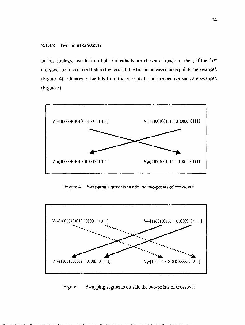
2.1.3.2 Two-point crossover
In this strategy, two loci on both individuals are chosen at random; then, if the first
crossover point occurred before the second, the bits in between these points are swapped
(Figure 4). Otherwise, the bits from those points to their respective ends are swapped
(Figure 5).
V1=[10000101010 101001 11011] V:z=:[11001001011 010000 01111]
V 1=[10000101010 010000 11011] V:z::[11001001011 101001 01111]
Figure 4 Swapping segments inside the two-points of crossover
V1=[10000101010 101001 11011]
······· ······ ······ ····· ....
V1=[11001001011 101001 01111]
V:z::[110010010 Il 010000 01111]
.. ..... . ····· ·······
••••• À ··~ V :z=[ 1 0000 1 0 1 0 1 0 01 0000 1 1 0 Il]
Figure 5 Swapping segments outside the two-points of crossover

Reproduced with permission of the copyright owner. Further reproduction prohibited without permission.
15
Since crossover requires two parent strings its power depends on the differences between
those parents; then, as the population converges, its power diminishes (Rana, 1999).
2.1.3.3 Multi-point crossover
It is an extension of two-point crossover where each string is treated as a ring of bits and is
divided by k crossover points into k segments. One set of alternate segments is exchanged
between the pair of strings to be crossed. Spears and Jong (1991) present an analysis of
the multi-point crossover.
2.1.3.4 Uniform crossover
Using this scheme, strings of bits rather than segments are exchanged. While traditionally,
single-point and two-point have been defined in terms of cross points or places between
loci where a chromosome can be split, both operators including uniform crossover can be
expressed using a crossover mask (Rana, 1999; Syswerda, 1989).
By applying a crossover mask, the parity of each bit in the mask decides which parent will
provide a bit to the corresponding position in a child. The mask-based crossover operations
are the sarne for each of the three different crossover operators and the differences lie in
the characteristic patterns (Figure 6).
Figure 6 shows that for either single-point or two-point crossover the 1-bits in the masks
are contiguous. whereas for uniforrn crossover, the 1-bits are not. ln fact, each position
in the rnask for uniform crossover is a 1-bit or O-bit with a uniforrn probability of 0.5.
Figure 7 presents an example of using a uniforrn crossover mask with two parents and
producing two children. For the first child, the O-bit in the mask rneans that is the first
parent who provides the gene at the corresponding position and the 1-bit rneans that is
the second parent who provides its corresponding gene. Conversely, for the second child
the O-bit in the mask leads to the second parent who provides the corresponding gene and

Reproduced with permission of the copyright owner. Further reproduction prohibited without permission.
viceversa.
Child 1:
Single-point: 111111 0000
Two-point: 0011111 ûOO
1100000111
Uniform: 0101101101
Figure 6 Exarnples of crossover masks
Parent 1 : 1 011 011 00
Parent 2: 0111 00011
Mask: 01 0101 001
111100101 Child 2: 001101 01 0
Figure 7 Uniform crossover operator
2.1.3.5 Positional and distributional biases
16
The advantages and drawbacks of crossover operators for genetic search are govemed by
the relationship between the positional and distributional biases, and the search problem

Reproduced with permission of the copyright owner. Further reproduction prohibited without permission.
17
itself (Rana, 1999). The first bias, positional one, refers to the frequency that bits that
are far apart on an individual will be separated by crossover than bits that are close to
gether (Wu and Garibay, 2002). As an example, suppose that the parent chromosomes
are 01110 and 10001, under one-point crossover it is possible to produce offsprings like
00001 or 10000 but never 00000 because the values at both the first and the last bit can
never be exchanged concurrent! y. The distributional bias refers to the number of bits that
are swapped under a specifie crossover operator (Rana, 1999). By using positional and
distributional biases definitions, it is possible to assert that while single-point crossover
exhibits the maximum positional bias and the least distributional bias, uniform crossover
has maximal distributional bias and minimal positional bias.
Empirical studies suggest a high degree of interrelation between the type of crossover im
plementation and the population size of the set of potential solutions. In the case of small
populations, uniform crossover is more suitable because of its disruptiveness; it helps
to sustain a highly explorative search, to overcome the limited information capacity of
smaller populations and the tendency for more homogeneity (De Jong and Spears, 1990).
However, for large populations, their inherent diversity diminishes the need for exploration
and therefore a less disruptive operator like two-point crossover is the best choice.
2.1.4 Mutation
This genetic operator ensures a more thorough coverage of the search space by stochas
tically changing the value of a particular locus on an individual (Figure 8). It prevents a
very early convergence of the population on local maximum or minimum by forcing an
individual into a previously unexplored area of the problem space. From a nature point of
view, mutation plays the role of regenerating lost genetic material produced by crossover
and selection operators.
For many problems, this operator is not generally considered as important as crossover

Reproduced with permission of the copyright owner. Further reproduction prohibited without permission.
18
V1=[1000010101010 1 00111011] ---•• V1=[1000010101010 0 00111011]
Figure 8 Mutation operator
and selection in the GA philosophy (DeJong, 1975; Goldberg, 1989), and a low mutation
rate (::::: 1/population_size) is often used. However, there seems to be a growing body
of practical problems where mutation plays a significant role (Beer and Gallagher, 1992;
Juric, 1994; Fogel and Atmar, 1990; Schaffer and al., 1989).
2.1.5 Fitness fonction
The objective function, the function to be optimized, provides the way to evaluate each
chromosome; however, its range of values is not the sarne from problem to problem. Then,
to maintain uniformity over different problem domains, the fitness function is usually
normalized to the range of 0 to 1. This normalized value of the objective function is really
the fitness of the string which the selection mechanism works with.
2.1.6 Selection
Selection mimics the survival-of-the-fittest mechanism found in nature (Srinivas and Pat
naik, 1994b ), where fitter solutions survive wh ile weaker ones perish. In other words, this
operator determines the actual number of o:ffspring each individual will receive based on

Reproduced with permission of the copyright owner. Further reproduction prohibited without permission.
19
its relative performance (Baker, 1987).
According to Baker (1987) the selection phase is composed of two parts (Baker, 1987):
1) determination of the individuals' expected values; and 2) conversion of the expected
values to discrete numbers of offspring. An individual's expected value is a real number
fd f indicating the average number of offspring that individual should receive. This means
that an individual with an expected value of 2.5 should average two and half offspring. For
sorne objective functions the computation of the expected value is not feasible because
of negative values; therefore, a mapping of the objective values to a positive domain is
necessary. In any case, the algorithm used to convert the individual expected values to
integer numbers of offspring is known as a sampling algorithm. According to Baker ( 1987)
a very good sampling algorithm should satisfy the following conditions:
1. Zero Bias. This means that the absolute difference between an individual's actual
sampling probability and his expected value must be zero.
2. Minimum Spread. If f('i) is the actual number of offspring individual i receives
in a given generation, then the "spread" is defined as the range of possible values
of f(i). Thus, smallest possible spread which theoretically permits zero bias is the
"Minimum Spread".
3. Not to increase the overall time complexity of the genetic algorithm.
In his work, he asserts that the "Stochastic Universal Sampling" algorithm (SUS) (see
Figure 9), which is analogous to a spinning wheel with N equally spaced pointers and a
complexity of O(n), is an optimal sequential sampling algorithm. Its use enables GAs to
assign offspring according to the theoretical specifications.
There are many different selection methods, and the best known (and used in developing
GAs) are described below. In the most general sense of the term, selection is an operator
that selects (according to sorne criteria) J.1 parents from À individuals.

Reproduced with permission of the copyright owner. Further reproduction prohibited without permission.
1. Compute the fitness average of the population
N f· faverage = L ~:
i=l
2. Compute the expected value of offspring
E.- fi 1-
faverage
3. Choose position of first marker: mark= rand();
4. Initialize accumulator of expected value of offspring: sum = 0:
5. Initialize counter of individuals: i = 0;
6. Repeat while i < N
(a) Increment accumula tor: sum = sum + Ei;
(b) vVhile mark < sum
i. Select the individual i
ii. Increment marker: mark = mark+ 1;
( c) Increment co un ter: i = i + 1;
Figure 9 Stochastic Universal Sampling Algorithm
2.1.6.1 Proportional Selection (or Roulette Wheel)
20
This method assigns a probability of being chosen proportional to its fitness. The main
disadvantage of this method is that when the population settles down and individuals have
similar fitness, the selection pressure decreases and then it does not work any better than
random selection. Also, negative fitness values tend to confuse the selection process.
While the conventional roulette wheel selection has difficulties in keeping graduai nar
rowing of the population, referred by Goldberg (1989) as the phenomenon of premature

Reproduced with permission of the copyright owner. Further reproduction prohibited without permission.
21
convergence, scaling of the fitness relaxes these problems; however, it requires adjustment
of the selection pressure by ti me consuming trial-and-error (Ki ta and Yamamura, 1999).
When the selective pressure is high, the search focuses on the top individuals in the pop
ulation and the genetic diversity is lost (too early convergence); on the contrary, if the
selective pressure is low the exploration increases and more genotypes are involved in the
search lowering the speed of convergence to an optimal (Baker, 1985; Whitley, 1989).
2.1.6.2 Ranking Method
This approach was proposed by Baker ( 1985) to overcome the above mentioned weakness.
First, the method sorts the individuals in the population according to their fitness, and
then, it applies a linear normalization method to compute the adaptation values for each
individual of the population as it is shown in Figure 1 O. Each individual in the mnk
receives a value between min and max following the expression:
where
and
!adaptation (rank) =a:· rank+ /3,
(max-min). a:= N- 1 , ,8=min
(ma..x- min) N-1
max= 17ma.x; min = (2.0 - 17min)
17ma.x + 17min = 2; 1 ::=:; 17ma.x ::=:; 2
(2.1)
Renee, the number of offsprings from a given individual is sol ely a function of its rank.

Reproduced with permission of the copyright owner. Further reproduction prohibited without permission.
22
fadaptation
max
min
N Rank
Figure 10 Linear norrnalization method
2.1.6.3 Geometrie Ranking Method
The geometrie ranking scheme sorts the individuals of the population by their fitness, and
then, computes the adaptation values for each individual of the population by using the
following geometrie norrnalization expression (Michalewicz, 1996):
r ( k) (1 )rank-1 J adaptation ran = c . q - q (2.2)
where q is the geometrie factor, and
1 c = -----,------:-
1- (1 _ qyank

Reproduced with permission of the copyright owner. Further reproduction prohibited without permission.
2.1.6.4 Tournament selection
In this selection method, k individuals (with replacement or without replacement) are
randomly picked from the population (k-tournament) at a time, and the one with the
best fitness is selected. The larger the tournament size, the higher the selection pressure.
Mathematical analysis of tournament selection with three schemes presented before can
be found in (Goldberg and Deb, 1991).
2.1.6.5 Truncation selection
ln truncation selection the candidate solutions are ordered by fitness, and sorne proportion,
p, (e.g. p=1/2, 1/3, etc.), of the fittest individuals are se1ected and reproduced 1/p times.
Truncation selection is less sophisticated than many other selection methods, and it is
commonly used in Breeder Genetic Algorithm (BGA) and in evolutionary strategies.
2.2 Real-Valued Genetic Algorithms
As the influence of Evolutionary Strategies (ES) (Beyer and Schwefel, 2002) has grown
stronger in the field of optimization, the use of real encoding has been also incorporated
in Genetic Algorithrns for real function optimization problems.
The use of real-valued GAs for real function optimization not only simplifies the prob
lem of coding phenotypes in genotypes, and decoding genotypes in phenotypes, allowing
GA's operators to work directly in the same domain without any mathernatical transfor
mation (Michalewicz, 1996), but also favars the use of multiple possible implementations
of crossover and mutation operators. In the following the operators used by RGA are
described.

Reproduced with permission of the copyright owner. Further reproduction prohibited without permission.
24
2.2.1 Crossover operator
Real-parameter crossover operators can be able to produce exploration or exploitation at
different degrees by handling the current diversity of the population. Either they gen
erate additional diversity, exploration, or use the current diversity to create better ele
ments, exploitation, or something in between. Let us consider x = { x1 , x2 , ... , Xn} and
y = {y1, y2 , •.. , Yn} be two elements of a populationp, where x.i and Yi can have values
in the interval [ai, bi]. Let us also say th at z = { z1, z2 , ..• , Zn} is an offspring of x and y
after a crossover operation. Now, if we set up Oi = min{ Xi, Yi} and /3i = max{ xi, Yi}
then the action interval [ai, bi] of these i's variables can be divided into three intervals:
[ai, o1], [ai, .Bi], and [.Bi. bi]· Thus, the value of a variable z1 will be bind to one of those
regions. Moreover, a crossover operation can produce a fourth region [a~, /3.;] with a~ :S ai
and ,BI ~ .Bi where zi can fall down. Herrera et al. (2003) name the region inside [oi, ,3i]
as exploitation zone; both regions outside the same interval as exploration zones; and the
region inside [a~, .B:J as a relaxed exploitation zone which combines the characteristics of
the other three (see Figure 11). Below we describe sorne crossover operators and present
their geometrie interpretation.
Relaxed Exploitation
Exploration Exploitation Exploration
1 1 1 1 1 f3i
Figure 1 1 Action intervals for crossover operators

Reproduced with permission of the copyright owner. Further reproduction prohibited without permission.
25
2.2.1.1 Discrete recombination (DR)
Each zi is randomly selected from the set {xi, Yi}- This corresponds to a standard uniform
crossover in the binary case. Geometrically it is represented in Figure 12. The probability
of choosing xi or Yi could also be specified, biasing the choice more towards one of the
parents.
0
@ 0
li Parent
Q Offspring
Figure 12 Geometrie Interpretation of DR
2.2.1.2 Blend Crossover (BLX- a)
This operator was proposed by Eshelman and Schaffer ( 1992). It creates offsprings ran
domly within a hyper-rectangular defined by the two parents. Consider the case when
the problem has only two variables, and suppose that the first parent has the position
(xr, x2), and the second parent (yr, y2) as it is shown in Figure 13. Let us call the interval
Ii = Yi - Xi and 0 < ai < 1 a random number; then each variable Zï of a new offspring
can be generated by randomly choosing a point within the interval

Reproduced with permission of the copyright owner. Further reproduction prohibited without permission.
1!!1 Parent
Ü Offspring
Figure 13 Geometrie Interpretation ofBlend Crossover-a: (BLX- a:)
2.2.1.3 Linear recombination (LR)
26
This operator is similar to BLX -a: but the value of O:i is the same for ali the genes i.
Thus, one of the offspring z(l) eould be given by:
z(l) =x+ a:(y -x) (2.3)
and the other by:
z<2) =y- a:(y- x) (2.4)
where a:> 0
The parameters a:' s could be fixed or ehosen randomly. If a: < 1 then the operator is also
known as Arithmetic Recombination. The geometrie interpretation of this operator using
two variables is presented in Figure 14.

Reproduced with permission of the copyright owner. Further reproduction prohibited without permission.
1!!1 Parent
Ü Offspring
Figure 14 Geometrie Interpretation ofLinear Crossover
2.2.1.4 Fuzzy recombination (FR)
ln this case (Voigt et al., 1995), the value Zi is given by a bimodal distribution:
with triangular probability distribution '1/J(r) having the modal values Xi and Yi with:
x· - dly·- x·l < r < x· - dly·- x·l 1 t. 1, __ 1, t 1
for xi ~Yi and d 2 ~- Geometrically, it is represented in Figure 15.
2.2.1.5 SBX
27
Similar to fuzzy recombination is simulated binary crossover, or SBX (Deb and Agrawal,
1995), where the children zY) and zfl are computed using the algorithm of Figure 16. Ge
ometrically, the probability distribution, which follows a shape sirnilar to the one presented

Reproduced with permission of the copyright owner. Further reproduction prohibited without permission.
28
Figure 15 Geometrie Interpretation of Fuzzy Crossover
in Figure 17, assures that when the parent values are far from each other it is possible to
generate children th at are far away from them; whereas, if the parent values are close from
each other then distant children solutions are not likely (Deb and Agrawal, 1999).
1. Generate a random number 'U E U(O: 1);
2. Compute
= {(2'U)'l!l 1
/3q ( 1 ry+l) 2(1-u)
Here 1] is sorne parameter.
if 'U :5 0.5
othenvise. (1)
3. Compute children zjU+1) and zf·t+1) from parents x~t) and Y?) using
the equations
(2)
(3)
If the variables are not within bounded demains (i.e. xf ~ xi ~ xf and yf ~ y1 ~ yf), the probability distributions need to be adjusted.
Figure 16 SBX algorithm

Reproduced with permission of the copyright owner. Further reproduction prohibited without permission.
a. 1
2.2.2 Mutation
x. 1
Figure 17 Shape of SBX's probability distribution
29
b· 1
A mutation operator similar to the common mutation for the binary case where only one
or two positions are flipped may be implemented. To do it, it is necessary to have closed
intervals for the domain of each variable and to defi ne a complementary operation in terms
of these intervals. However, in practice we found this very ineffective. Hence, more
interesting mutation types have been used:
2.2.2.1 Uniform Random mutation
Once a variable is selected for mutation, choose a uniform random value within its range
and assign this value to the variable. Thus, every value is possible.
2.2.2.2 Non-Uniform mutation
Janikow and Michalewicz ( 1991) experimented with a simple deterministic control scheme
which they called nonuniform mutation. In this approach, one variable xk is selected ran
domly, and its value is set to a random number following the expressions (2.5) and (2.6)

Reproduced with permission of the copyright owner. Further reproduction prohibited without permission.
xt+l = { x~+ ~(t, T(k) - xk) if r < 0.5, k x~- ~(t,xk -l(k)) if r > 0.5,
where
T represents a uniforrn random numberbetween (0, 1),
t is the current generation,
T is the maximum number of generations,
b is a shape parameter, and
r(k), l(k) are the upper and lowerborders of xk.
30
(2.5)
(2.6)
The idea behind this type of mutation is the following: at the beginning of the search,
large jumps are necessary to explore the solution space; but as the search progresses,
small jumps are more desirable for finetuning. Figure 18 displays the value of~ for three
selected times illustrating the behavior of the operator.
2.2.2.3 Gauss mutation
This type of mutation is similar to the previous one with the only difference that the mu
tation step ~i follows a Gauss distribution)\( ( 0, a) as it is described by:
1 ( [x[ ) P(x) = ~ e -z;:r
(27ïa) 2 (2.7)
where n is the number of dimensions.
The a parameter does not only control the ratio of height to width but also corresponds to
the variance of the distribution. As it can be seen in Figure 19, this distribution has a fini te
range and it is much likely to generate smaller mutation steps than large mutation steps.

Reproduced with permission of the copyright owner. Further reproduction prohibited without permission.
x [y]
r-----------~--~--~--~--~--~--~--·
0.7 ..
0.6 \
o.s .. ,
0.4 ..
0.2
... : ,:
.... -~~' ... ... ..... ~.~., ...
0.1 ":-~-~-~·········~·
Figure 18 .6. ( t, y) for three selected ~ values and b = 5
12r-----~----,------r----~-----,----~~----r-----~----,-----,
10 .......
8 ...... .
~ 6 ......
"'" 4 .......
2 ......
. ... ~ ..
~~~-----~o~.s~c:~~----~o~.4-----o~.2~--~o-----o~.~2-----o~.4----~~=--o~.-s----j x
Figure 19 ID Gaussian distribution (u = 0.23)
31

Reproduced with permission of the copyright owner. Further reproduction prohibited without permission.
32
2.2.2.4 Cauchy mutation
This type of mutation follows a Cauchy distribution as the one illustrated in Figure 20 and
described by:
(2.8)
where Nn is a normalization constant, and n is the number of dimensions.
While Gauss distribution decays exponentially, the Cauchy distribution decays like ;'2 for
large x. Contrary to the Gauss distribution the parameter CT controls the ratio of height to
width, but it does not correspond to its variance which is infinite (Kappler, 1996). As we
can observe in Figure 20 this mutation operator can be capable of larger jumps than the
Gaussian mutation operator.
~~~----0~.8~--~0~.6--~-0~.4~--~0.~2--~0--~0.~2--~0~.4~~0.~6---0~.8~~ x
Figure 20 ID Cauchy distribution (CT= 0.30)
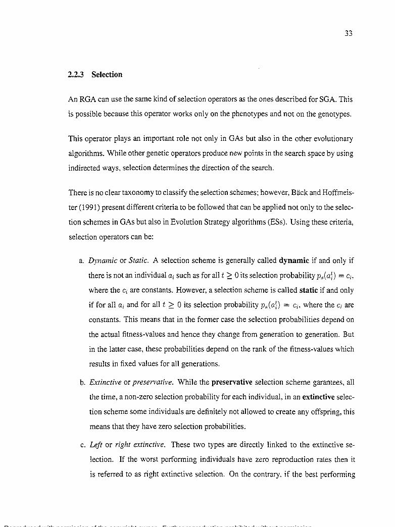
Reproduced with permission of the copyright owner. Further reproduction prohibited without permission.
33
2.2.3 Selection
An RGA can use the same ki nd of selection operators as the ones described for SGA. This
is possible because this operator works only on the phenotypes and not on the genotypes.
This operator plays an important role not only in GAs but also in the other evolutionary
algorithms. While other genetic operators produce new points in the search space by using
indirected ways, selection determines the direction of the search.
There is no clear taxon orny to classify the selection schemes; however, Back and Hoffmeis
ter ( 1991) present different criteria to be followed th at can be applied not only to the selec
tion schemes in GAs but also in Evolution Strategy algorithms (ESs). Using these criteria,
selection operators can be:
a. Dynamic or Static. A selection scheme is generaily calied dynamic if and only if
there is not an individual ai such as for ali t 2:: 0 its selection probability ps(aD =ci,
where the Ci are constants. However, a selection scheme is called static if and only
if for ali ai and for ail t 2:: 0 its selection probability Ps (aD = ci, where the ci are
constants. This means that in the former case the selection probabilities depend on
the actual fitness-values and hence they change from generation to generation. But
in the latter case, these probabilities depend on the rank of the fitness-values which
results in fixed values for ali generations.
b. Extinctive or preservative. While the preservative selection scheme garantees, ail
the time, a non-zero selection probability for each individual, in an extinctive selec
tion scheme sorne individuals are definitely not allowed to create any offspring, this
means that they have zero selection probabilities.
c. Left or right extinctive. These two types are directly linked to the extinctive se
lection. If the worst performing individuals have zero reproduction rates then it
is referred to as right extinctive selection. On the contrary, if the best performing

Reproduced with permission of the copyright owner. Further reproduction prohibited without permission.
34
individuals are prevented from reproduction then a left extinctive selection takes
place. This last scheme is very rare in practice but its effect is to avoid premature
convergence due to super-individuals.
d. Elitist or pure. While in an elitist selection scheme sorne or ail the parents are
allowed to undergo selection with their offspring (Jang, 1975), the pure scheme
enforces a life ti me of just one generation for each individual regardless of its fitness.
e. Generational or steady-state. In the generational selection scheme the set of par
ents is fixed until À offspring are produced and then the new set of offspring replace
the last generation. In the case of steady-state selection an offspring immediately
replaces a parent if it performs better, generating the possibility that the set of par
ents may change for every reproduction step (Whitley, 1989).
While the proportional selection scheme can be characterized as a dynamic and preser
vative selection, linear ranking, geometrie ranking and tournament selection schemes are
static and preservative. Only truncation selection is extinctive. The last two criteria can be
implemented in any of the selection schemes.
2.3 Macroscopic view of the search process of GAs
A few studies (Ki ta and Y am amura, 1999; Kita, 2001) suggested the ideas th at GAs should
be designed to maintain the diversity of the population and to inherit good characteristics
from parents. During the search process of the GAs, an initial population is randomly
chosen. Then, operators that use random numbers like selection, crossover and mutation
operators are applied repetitively to the population transforming its probability distribution
function (pdj) like a very natural evolution process. While selection operation narrows the
pdf by selecting and duplicating individuals having higher fitness, the crossover operation
generates children and transforms the pdf by corn bining the information of parents. If the
crossover still narrows the pdf of the population then the search would be focused on a
smaller region than the one specified by the selection. On the other hand, if the crossover

Reproduced with permission of the copyright owner. Further reproduction prohibited without permission.
35
enlarge too rouch the pdf, it would work on regions that have been already eut out by
the selection. Th us, the crossover operator should preserve the pdf of the population to
exploit the current region. To this process it has to be added that the mutation operation
also enlarges the pdf by giving a perturbation to each individual.
Following this reasoning, Kita and Yamamura (1999) propose an hypothesis, named func
tional specialization hypothesis, for the selection and crossover operators:
"In the GA, selection operation should be designed so as to gradually narrow the pdf of the population, and the crossover operation should be designed so as to preserve the pdf while keeping its abi1ity of yielding novel solutions in finite population case."
Based on empirical findings and the functional specialization hypothesis ((Kita and Yama
mura, 1999; Ki ta, 2001 )), the au thors elaborated the following guidelines for the design of
crossover operators for RGAs:
Guideline 1. The crossover operator should preserve the statistics of the population
such as mean vector and the variance-covariance matrix. It should be
noted that preservation of the covariance is important to achieve good
performance in optimization of non-separable functions.
Guideline 2. Crossover operators should generate offspring having as rouch diversity
as possible under constraint of Guideline 1.
Guideline 3. Guideline 1 is useful when the selection operator works ideally. However,
it may fail to suggest a good region to be searched by the population. To
make the search robust, children should be distributed more widely than
in Guideline 1. It should be noted that the Guideline 1 gives a reference
point, and there exists a trade-off between efficiency and robustness in
adopting this guideline.

Reproduced with permission of the copyright owner. Further reproduction prohibited without permission.
36
Bey er and Deb (200 1) postulate two properties th at the crossover should have for success
ful applications in RGAs:
a. The crossover operator must produce a children population that has the same mean
as that in the parent population;
b. The variance of the resulting children population may be larger than that of the
parent population.
As we can observe these two properties are in line with the Guidelines proposed by Kita
and Yamamura ( 1999). In fact, Herrera et al. (2003) highlight that Guideline 1 supports the
importance of considering the exploration and relaxed exploitation intervals for designing
crossover operators for RGAs (Figure 11).
2.4 Other Evolutionary Computation Algorithms
Many different types of evolutionary algorithms exist; however, genetic algorithms and
evolution strategies are two of the most basic forms of evolutionary algorithms. While
genetic algorithms used binary coding at the beginning and recombination is emphasized
over mutation, evolution strategies have used more direct representations (Back et al.,
1991) since its beginnings and mutation is emphasized over recombination. Although both
genetic algorithms and evolution strategies have been used for optimization, GAs have
long been viewed as multipurpose tools with applications in search, optimization, design,
and machine leaming (Bolland, 1992; Goldberg, 1989) and most of the work in evolution
strategies has focused on optimization (Back, 1996; Schwefel, 1981, 1995b ). During the
last decade, these two fields have influenced each others and many new algorithms have
freely borrowed ideas from both traditions (Whitley, 2001).
Evolution Strategies (ESs) were introduced by Rechenberg at Berlin in the 1960's and
further developed by Schwefel (Back et al., 1991 ). ESs were applied first to experimental
optimization problems with more or less continuously changeable parameters only. The

Reproduced with permission of the copyright owner. Further reproduction prohibited without permission.
37
applications dealt with hydrodynamical problems like shape optimization of a bended pipe
and of a flashing nozzle, or with control problems like the optimization of a PID regulator
within a highly nonlinear system. The algorithm used in these applications was a simple
mutation-selection scheme called two membered ES. It was based upon a "population"
consisting of one parent individual (a real-valued vector), and one descendant, created by
means of adding normally distributed random numbers. The better of both individuals
then served as the ancestor of the following iteration/generation.
In ESs, each individual is represented as a pair of real-valued vectors (xi, T!i), where xi is
a vector of object variables, T/i is a vector of its strategy parameters, and i E {1. .... p}.
The general form for real-valued parameter optimization problems is (p,j p-+;).) - ES
where ). > f.-L ;::: p ;::: 1. (p/ p-+; >.) means that p parents generate ). offsprings through
recombination (p ;::: 2) and mutation at each generation. p is the number of parents to
form one new offspring using recombination. The case where p > 2 is known as multi
parent recombination. If"," is used instead of"+" then the best f.L children become the
next generation of parents. On the contrary, if"+" is used then the best p individuals of
both: parents and children become the next generation of parents. This means that the À
children together with the p parents are sorted by their fitness value and then only the first
f.-L individuals are selected.

Reproduced with permission of the copyright owner. Further reproduction prohibited without permission.
CHAPTER3
PROBLEM DESCRIPTION
Before describing the methodology used along this research, it is highly important to know
with more detail the application problem with which we will test our new GAs. So, this
chapter explains the type of problem we are dealing with. We start by describing the
architecture of the flight control system architecture of an aircraft. Then, we present the
definitions for the handling qualities criteria to be satisfied by the flight control system.
And finally, we explain the way a cost function is derived using the handling qualities, and
the optimization approach used in conjunction with GAs to solve our problem.
3.1 Architecture of the Flight Control System
We are interested in the design of a longitudinal controller capable of tracking pitch-rate
commands with predicted Level 1 (Mclean, 1990) handling qualities and desired time
domain response behaviors. In other words, the closed-Ioop response, from pilot pitch rate
commands to resulting pitch rate, must follow the reference model response as close1y as
possible.
Figure 21 corresponds to the architecture of a longitudinal flight control system presented
that we will use in our problem (Zhu et aL 2000). In this model, the aircraft block rep
resents the characteristics of aircraft system provided by Bombardier. The control system
is composed of a stability augmentation loop and a proportional-integral (Pl) plus feed
forward control augmentation loop where only the controller gains Kff, Ki, Kp, Kn::' and
Kfb are adjustable. The output of the system, q, represents the pitch rate of the aircraft
and nz is the normal acceleration.
The design of stability augmentation system of the longitudinal flight control system is
performed using the classical approach by first dividing the flight envelope into a num-

Reproduced with permission of the copyright owner. Further reproduction prohibited without permission.
39
Il ---~· K 1
1
1-"ll ~ .. -.[1 ;:-.1 tl4ff~Tl1 oo.mo• ~'-: -A-Irc-raft_-
11q
li l li 1
' K ; ( \:LJ K L---J n,__j
1
P 1 ~ ,. l 1 Tms.,. 1
·- 1 1 1 -- ! ~ 1 '
l' !l !
--. K,b ~ ~ j 1 1 Tws...1 ~ ~1 --~
Figure 21 Architecture of longitudinal flight control system
ber of sub-domains based on sorne characteristics like Mach number, altitude, center of
gravity, weight and others. Then, for each operation point or sub-domain, the model is
linearized for its study and simulation. For simulation purposes of the longitudinal flight
control system, the aircraft can be represented by the state equation 3.1:
x= Ax+Bu (3.1)
with
x~[i], [ x. Xw 0
-gCOS'(o l Zu Zw Uo -g sm '"Yo
A~ A~. Afw AÏ J\;Ie ' q
0 1 0
and

Reproduced with permission of the copyright owner. Further reproduction prohibited without permission.
40
when the aircraft is being controlled only by means of elevator deflection. 6E. In ether
words when,
The states variables u, w, q and e denote forward speed, vertical velocity, pitch rate and
pitch attitude respectively, and Xu, Xw, Zw Zw, .!',:fu. 1Üw, represent the stability deriva
tives.
3.2 Handling Quality Requirements
According to Harper Jr. and Cooper (1986), handling qualities are
''those qualities or characteristics of an aircraft that govem the ease and precision with which a pilotis able to perform the tasks required in support of an aircraft role"
By addressing handling qualities, ftight control system designers are able to identify the
requirements and the constraints needed for the definition of the objectives of flight control
system and evaluation of the design results. While a handling quality study is concemed
with the pilot and aircraft interface, a flight control system design is related with how
to correct the characteristics of aircraft though a control system such that the specifica
tion of handling qualities can be satisfied when the pilot "interfaces" the aircraft (Etkin,
1959). The following sections exp lain each one of the handling qualities criteria used in
our model.
3.2.1 Bandwidth Criterion and Phase Delay
The definition ofbandwidth for flying qualities is different from that used in most general
purpose control texts (Hodgkinson, 1999). Using the frequency response of attitude to
pilot's control input (Figure 22), the bandwidth parameter is defined as the smaller of two

Reproduced with permission of the copyright owner. Further reproduction prohibited without permission.
41
frequencies, the phase-limited bandwidth WBWPH or the gain-Iimited bandwidth WBWG·
The fi.rst one is the frequency where the phase margin is 45°; and the second one is given
by the frequency at which the gain margin is 6dB relative to the gain when the phase is
180°. From a pilot's point of view, aircraft with high bandwidth frequencies tend to have
crisp, rapid, and well-damped response, while aircraft with low bandwidth frequencies
tend to wallow and have sluggish responses.
The phase delay, Figure 22, is related to the slope of the phase between the crossover
frequency and 2w180. It is defi.ned as:
~~2WJSO T - -----=c:..:.....-
p - 57.3 x 2w1so
0 ..................... .
Gain( dB)
-20
-100~:::-: ... ,.... --...;.;;;.;...= --+ 45" -----Phase(deg) -200
-300 . . 't p
~<I>
57.3 X 2(J)1 XO
Frequency (rad/sec)
Figure 22 Definition of Bandwidth and Phase Delay.
(3.2)

Reproduced with permission of the copyright owner. Further reproduction prohibited without permission.
42
3.2.2 Flight Path Delay
This criterion states that the ftight path delay, as defined in Figure 23, should be small;
preferably below 1 second. The ftight path delay as function of the response parameters
is:
(3.3)
where (spis the short period mode damping ratio, and Wsp is the undamped frequency.
e.y,q
e
q
Drb/ q_,.__. 2 4 6
r(sec)
Figure 23 Pitch response criterion.
3.2.3 Dropback Criterion
The dropback criterion is a measure of the mid-frequency response to attitude changes.
Excessive dropback results in pilot complaints of abruptness and lack of precision in pitch

Reproduced with permission of the copyright owner. Further reproduction prohibited without permission.
43
control - complaints corn mon also to aircraft with excessive values of pitch attitude band
width.
The criterion of Gibson dropback requires a step pitch manipulator input, be , be applied
until a steady state pitch rate, qss , is reached. The measure of dropback is shown in
Figure 23. Since the path time delay, t1 , is given by equation (3.3), the relationship for
dropback can be derived as:
Drb _ ~ 2(sp ---lq __ _
qss Ulsp (3.4)
where qss is the steady state pitch rate, and 1/Tq defines the flat region of the attitude-tc
stick bode plot. Moreover, Terminal ftight phase Gibson dropback criterion boundaries is
defined by:
Drb -0.25 <- < 0.5(sec)
qss
3.2.4 CAP Criterion
The Control Anticipation Parameter, or CAP for short, was first used in the United States
military handling qualities specifications. It connects the short period natural frequency
and the normal acceleration due to a change in angle of attack, in the following way:
(3.5)
where n=o is the normal acceleration per unit angle of attack.
The magnitude of CAP gives an indication of the change in steady-state normal accelera
tion from the aircraft's initial pitching acceleration. This is essential because of the time
lag between the pilot's input and the final steady-state normal acceleration. For a linear
aircraft model, this parameter can be calculated using the following formula:

Reproduced with permission of the copyright owner. Further reproduction prohibited without permission.
n. V n .. =--=::::::::--o
where V is the true air speed and g is the acceleration due to gravity.
44
(3.6)
The handling quality criteria considered in this work are pitch attitude bandwidth w s11·,
phase delay T P' short period mode damping ratio ( sp, and Gibson dropback DB. The
boundaries of these criteria are defined by MIL-STD-1797 A (Government, 1990) and they
are summarized in Table I.
Table I
Handling Qualities (HQs) and Performance Specifications
HQs & Performances Must Achieve Ideal
Attitude Bandwidth wsw > 1.5( radj sec) > 1.75
Phase Delay Tp < 0.2(sec) < 0.14
Short Period Mode Damping Ratio (sp 0.35 < (sp < 1.35 0.75 < (sp
Long Period Mode Damping Ratio (ph 0.05 <(ph 0.1 <(ph
Gibson Dropback DB -0.2 < DB!q,, < 0.5(sec) 0.0 < DB!q_.s < 0.3(sec)
3.3 Optimization Models of the Problem
A general formulation for an optimization problem can be expressed as:
min{f(x)lxz ~x~ xu; h(x) = 0; g(x):::; 0} xE Rn
where
Rn : n-dimensional Euclidean space;
f: objective function;
x: vector of n design variables;
g: vector of p inequality constraints;
(3.7)

Reproduced with permission of the copyright owner. Further reproduction prohibited without permission.
45
h: vector of q equality constraints; and
Xz, xu: lower and upper bounds of design variables (side conditions).
The design variables and the constraints expressions define the feasible space of the solu
tions of the problem (equation 3.8).
(3.8)
This general formulation can be modified in such a way that when there exists no con
straints we have an unconstrained optimization problem; otherwise, we have a constrained
optimization problem. The formulation of an optimization problem also changes depend
ing on whether there is only one objective function f(x), which can be expressed as scalar
optimization; or there are several objectives that must be considered simultaneously, which
can be modelled as a multiple objective optimization problem and the formulation of equa
tion (3.7) changes to:
mRin{F(x)Jxz ~x~ xu; h(x) = 0: g(x) ~ 0} xE n
(3.9)
where
F(x) = (f1(x), h(x),
is now a vector of k objective functions.
Although we have a problem with a vector of multiple objectives, it can be solved by
means of a substitute scalar optimization problem. A technique frequently used is to
express the vector of multiple objectives as a positive! y weighted convex sum of the ob
jectives, that is:
k
min L a:di(x), 0 ~ a:i < oo. x en
i=l
(3.1 0)

Reproduced with permission of the copyright owner. Further reproduction prohibited without permission.
A variation of this technique is the Mean/Deviation formulation which reads:
min (> .. P + ŒF), x en
where
k k - 1""' F = k~fi(x), ŒF = L (fi(x)- P) 2,
i=l i=1
and ..\ is a positive constant.
3.3.1 Unconstrained Optimization Model
46
(3.11)
In our first attempt to mode] the fly-by-wire problem, we have expressed the flight control
system design as an unconstrained optimization one, where the objective function is a
linear combination of functions associated with each one of the handling qualities criteria
with constant weights equal to one:
n
fcost = Lfi i=l
(3.12)
fi is a function associated with the handling quality i. The corresponding value of fi is
obtained each time that we use the simulation model for evaluating the behavior of the
system for a set of controller gains.
Currently we are using the evaluation functions included in the simulation mode] of a
business jet aircraft provided by Bombardier Aerospace. In this model, each handling
qualities criteria has been expressed as a sigmoid evaluation function. This type of smooth
function gives a value of 0 when a performance cri teri on of a given design takes the ideal
value, while tends to 1, when the performance moves away from the ideal value.
The example shown below illustrates the use of sigmoid function for one of the handling
qualities:

Reproduced with permission of the copyright owner. Further reproduction prohibited without permission.
47
Dropback: the evaluation function for the dropback is
!DB= 1- sech (AIDE- O.lJB) (3.13)
where A and B are constants provided by the design engineer. The corresponding
graph is shown in Figure 24.
Figure 24 Evaluation Function of Dropback
The cost function implemented in this way is highly nonlinear; to observe to a certain
degree the complexity of the function 3-dimensional graphies are shown in Figures 25 and
26. To construct these graphies we used the controller gains K 11 and Ki as variables and
the others Kprob, Knz and Ktb were fixed.
In Figures 25 and 26, we can apprecia te the nonlinearities of the cost function along the
gains Ki and Kff while the others gains are constants. lt is also possible to observe
the nonlinearities along the other gains when the two figures are compared and we have
changed the values of Kprob and Knz·

Reproduced with permission of the copyright owner. Further reproduction prohibited without permission.
3.5
2.5
2 2
Ki
···T·· ..
5
0 0 Kf!
Figure 25 Cost function with (Kprob, Kn:;, KJb) = (0.5, 0.5, 0.0)
4
3
0 2
Ki 0 0
..... -~ ....
.... -~
··· .. ~
5
Kf!
Figure 26 Cost function with (Kprob, Kn:;, KJb) = (0.03, 2.94, 0.00)
48

Reproduced with permission of the copyright owner. Further reproduction prohibited without permission.
CHAPTER4
LITERATURE REVIEW
The objective of this chapter is twofold: first, it outlines the major research activities
that have been presented for the research community in the areas of the application of
Evolutionary Algorithms to Aircraft Control System Design; and, second, it presents a
simplified review of the principal theoretical and experimental work relevant to different
techniques that the GA community has been using to solve mathematical problems with
constraints, as weil as, to implement Adaptive GAs. This chapter is ordered in three major
sections. While there exists a significant literature about the use of EAs in Aerospace
System design in general, section 4.1 only reports those works that are only related with
the application of EAs to ftight control system design. Section 4.2 of this chapter does
a review of the different methods that has been using to solve mathematical problems
with constraints. It concentrates in describing two types of techniques: based on penalty
functions, and based on feasibility criteria. Finally, Section 4.3 describes the application
of different adaptive techniques to control the parameters of GAs.
4.1 Applications of EAs to Aircraft Control System Design
During the last twelve years, Evolutionary Computation methods have been applied to
different types of Aircraft Control System Design problems. Here, without claiming to be
an exhaustive review of the domain. we present a short description of the key contributions
on ftight control design reported from 1992 to 2003. The emphasis in this description is
on the kind of GAs architecture that has been used, and what kind of fitness function has
been used in order to show the relevance and importance of the contributions of our work.
In Porter (1993), a GA is applied to the design of multivariable flight-control systems
using eigenstructure for a fighter aircraft meeting the performance requirements of MIL
F-8785C. The objective function is defined as a measure of eigenstructure error of the

Reproduced with permission of the copyright owner. Further reproduction prohibited without permission.
50
form:
n n
é = LÀilcria)- O"id)l + Lf.Lillv}a)- v}d)ll (4.1) i=l j=l
where Ài and f.Li are real non-negative weighting parameters, 1-1 is the modulus of a num
ber, 11-11 is an appropriate vector norm, the sets of crja) and crjdl are the actual and desired
eigenvalues, and the sets of vja) and vjd) are the actual and desired eigenvectors respec
tively. Porter (1993) reports the results for only one flight condition.
In Porter and Hicks (1994a,b, 1995a,b), the authors apply GAs to tune digital PID con
trollers of a model-following flight-control system for a fighter aircraft under diverse con
siderations, like open-loop, using different performance measures for GAs. They present
results for three flight conditions using two different objective functions: the first func
tion is implemented by computing the minimum difference between non-asymptotically
optimal and asymptotically optimal desired eigenvalues locations, and the second one con
siders the minimum maximum generalized closed-loop tracking error (Porter and Hicks,
1994b).
Chen and Cheng (1998) app1y a genetic approach to the design of a structure-specified con
troller to achieve H 00 optimal control purpose for a MIMO super-maneuverable FIS/HARY
fighter aircraft system. The controller parameters ei are coded as binary strings. The au
thors use a cost function E(e)
E(e) = supa(w) (4.2) 'Vw
to simultaneously minimize the robust stability performance and the disturbance attenua
tion performance proposed in (Kwakernaak, 1985; Francis, 1987; Stoorvogel, 1992) and

Reproduced with permission of the copyright owner. Further reproduction prohibited without permission.
51
included in the function a(w). Then, the cost function is scaled and transformed in the
fitness function:
F(e) = kE(e) + h (4.3)
where, using linear scaling,
(4.4)
(4.5)
Ew and Eb are the largest and smallest values of the cost function evaluated in the gen
eration, and Fw and Fb are the corresponding fitness values. As it can be observed from
the value of k, the minimization problem is transformed in a maximization problem when
F(e) is used.
Sweriduk et al. (1998) use genetic algorithm in the design of Hoc controllers for the lon
gitudinal and lateral-directional channels of a high-performance aircraft by selecting the
weighting functions. Their fitness criterion is determined by comparing the closed-loop
response with a Level 1 flying qualities model, which are defined with reference to the
ratings of 1, 2 and 3 of the Cooper-Harper scale (Harper Jr. and Cooper, 1986). The
weighting functions depend on free parameters:
K(n) = ui · u1 (4.6)
where
ui = L ... , 9, 10°, w- 1, 10-2 , 10-3 , 10-4 , 101, 102; (i = L ... , 16).

Reproduced with permission of the copyright owner. Further reproduction prohibited without permission.
They are coded as alphanumeric strings instead of binary strings of fixed length. Thus,
their GA works with 256 discrete values for each free parameter.
Crawford et al. (1999) use genetic search techniques to target four aerospace control de
sign problems, including homing missile guidance law synthesis, spacecraft reorientation,
and control and guidance of an A-4D aircraft. The authors report a very interesting ap
proach where several hand-derived control laws based on standard methods plus several
nonsensical controllaws are encoded.
Aranda et al. (2000) report the design of a controller for the Research Civil Aircraft Model
(RCAM) benchmark problem by using an evolutionary algorithm. They model the prob
lem as the optimization of multiple objectives like closed-loop stability, ride quality cri
teria, control activity criteria and robustness criteria. The components of the controller
matrices are encoded using ftoating point. To evaluate the individuals of a population they
use a Pareto-based ranking approach (Fonseca and Fleming, 1998) in combination with a
toumament selection method.
Table II summarizes the type of operators reported. The columns X over, AI utation and
Selection show the type of crossover, mutation and selection operator respectively; and
Enc indicates the type of encoding mechanism implemented.
Table III summarizes the parameters' values used in each of the works reported before.
The column "Type" refers to the kind of scheme used to produce the next generation and
has two possible values: Gis for a generational scheme, and SS is for steady state. N is
the number of chromosomes in the generation; Pc and Pm are the probability of crossover
and mutation respectively; and finally, Gen is the maximum number of generations that
the algorithm produces before to stop.
As we can observe, sorne authors did not present information about the type of crossover,
mutation and selection operator they used, neither there is analysis about the relationship

Reproduced with permission of the copyright owner. Further reproduction prohibited without permission.
53
Table II
Summary of type of operators and encoding mechanism
Ref. XoYer Mutation 1 Selection 1 Enc 1
Porter (1993) NR NR NR
Porter and Hicks ( 1994a), Porter and Hicks ( 1994b ),
NR NR NR Porter and Hicks ( 1995a), Porter and Hicks ( 1995b)
Sweriduk et al. ( 1998) NR NU Randorn
Chen and Cheng ( 1998) One-point Uniforrn Proportional
Crawford et al. ( 1999) 1
NR NR NR
Aranda et al. (2000) Simple, Arithrnetic, NonUniforrn, Tou marnent
Heuristic, and Multiple Randorn
N R =not reported; B = binary; F = jloating point; .4. = alphanumeric.; NU = it was not used.
Table III
Su rn mary of parameters' values
Ref. 1 Type 1 N 1 Pc 1 Pm Gen
Porter (1993) G 40 0.6 0.001 200
Porter and Hicks (1994a), Porter and Hicks ( 1994b ), G 50 0.6 0.002 150 Porter and Hicks (1995a), Porter and Hicks (1995b)
(Sweriduk et al., 1998) ss 500 NR NU 1000
(Chen and Cheng, 1998) G 100 0.9 0.2 200
(Crawford et al., 1999) G 500 NR NR 5000
(Aranda et al., 2000) G NR NR NR 1000
N R = Not reported; NU = it was not used; G = gene rational; S S = steady state.
B
B
A
B
B
F

Reproduced with permission of the copyright owner. Further reproduction prohibited without permission.
54
among the GA's parameters, its performance, and the tirne of execution. Moreover, none
of them used or defined the fitness function by directly computing the handling qualities
criteria. While the definition of the fitness function by using the handling qualities cri
teria was originally incorporated in the simulation model provided by Bombardier, the
experiments and the results produced by this research using this approach are already a
contribution to the research community.
Despite the promising results obtained in the application of GAs to system control de
sign for aircraft none of them mentions or elaborates any aspect related to reducing the
execution time and increasing the effectiveness of GAs. In fact, Sweriduk et al. (1998)
highlighted the need of doing a more exhaustive analysis of the effects of genetic param
eters in flight-control problems, and that the fitness should be defined by directly comput
ing handling qualities metrics, similar to the NASN Army code CONDUIT. Furthermore,
Krishnakumar et al. ( 1995) suggested the possibility of using GA with adaptive character
istics to find the way of improving GAs' performance.
4.2 Constrained Nonlinear Global Optimization using GAs
Using an unconstrained nonlinear global optimization model is not the only way of work
ing with GAs in order to find the best controller gains of a flight control system for a
business jet. It is also possible to use a constrained nonlinear optimization model and
apply GAs. Several techniques have been proposed by the GA community to solve math
ematical problems with constraints. In this section, we do a simplified review and analysis
of those more representatives. The present study is not complete in the sense that the
search of documentation has not been exhaustive and the experimentations of every arti
cle have not been repeated; however, the results that we present serve as a reference to
highlight the importance of our contributions.
A general definition for a nonlinear optimization problem can be formulated as finding
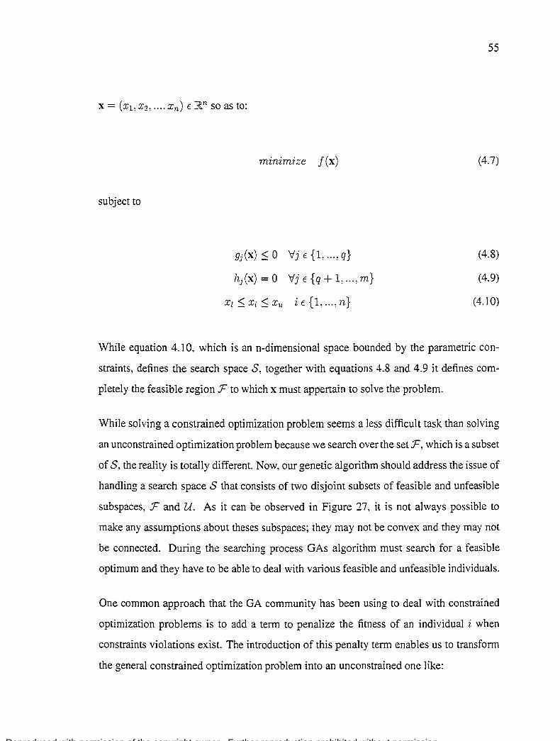
Reproduced with permission of the copyright owner. Further reproduction prohibited without permission.
X= (xl, X2, ... , Xn) E JRn SO asto:
subject to
m'inimize j(x)
gj(x) ::; 0 'tfj E {1, ... , q}
hj(x) = 0 'tfj E {q + 1, ... , m}
XL::; Xi::; Xu i E {1, ... , n}
55
(4.7)
(4.8)
(4.9)
(4.1 0)
While equation 4.1 0, which is an n-dimensional space bounded by the parametric con
straints, defines the search space S, together with equations 4.8 and 4.9 it defines com
pletely the feasible region :F to which x must appertain to solve the problem.
While solving a constrained optimization problem seems a less difficult task than solving
an unconstrained optimization problem because we search over the set :F, which is a subset
of S, the reality is totally different. Now, our genetic algorithm should address the issue of
handling a search space S that consists of two disjoint subsets of feasible and unfeasible
subspaces, :F and U. As it can be observed in Figure 27, it is not always possible to
make any assumptions about theses subspaces; they may not be convex and they may not
be connected. During the searching process GAs algorithm must search for a feasible
optimum and they have to be able to deal with various feasible and unfeasible individuals.
One common approach that the GA community has been using to deal with constrained
optimization problems is to add a term to penalize the fitness of an individual i when
constraints violations exist. The introduction of this penalty term enables us to transform
the general constrained optimization problem into an unconstrained one like:

Reproduced with permission of the copyright owner. Further reproduction prohibited without permission.
56
search space S
unfeasible search space U
Figure 27 A search space and its feasible and unfeasible parts
·tb(x) = j(x) + penalty(x) (4.11)
The penalty term extends the domain of the objective function which may transforrn a
smooth search landscape into a rugged one and it may influence the relative fitness of
individuals in a population. This penalty terrn does not only represent a penalty for an
unfeasible individual i, but also a cost for repairing such an individual (i.e. the cost for
making it feasible ).
Designing a penalty function is not an easy task and much of the difficulty arises wh en
the optimal solution lies on the boundary ofthe feasible region. Richardson et al. (1989)
suggest the following guidelines to derive good techniques to build penalty functions:
1. Penalties which are functions of the distance from feasibility are better perforrners
than those which are only functions of the number ofviolated constraints.

Reproduced with permission of the copyright owner. Further reproduction prohibited without permission.
57
2. For a problem having few constraints, and few fully feasible solutions, penalties
which are solely functions of the number of violated constraints are not likely to
produce any solutions
3. Good penalty functions can be constructed from two quantities: the maximum com
pletion cost and the expected completion cost. The completion cost is the cost of
making feasible an unfeasible solution.
4. Penalties should be close to the expected completion cost, but should not frequently
fall below it. The more accurate the penalty, the better will be the solution found.
When a penalty often underestimates the completion cast, then the search may fail
to find a solution.
While these guidelines can be useful for designing, they are difficult to follow in many as
pects, especially because the maximum completion cost and the expected completion cost
may not be known before the optimization. Generally the penalty function is composed
by a sequence of penalty coefficients Ri defined by the user and a function rjJ, which is a
measure of ali the constraints violations produced by the unfeasible individual and can be
greater or equal to zero.
(4.12)
Most of the methods using penalty functions use the following quadratic loss function
(Fiacco and McCorrnick, 1968) to express the constraint violation measures:
(4.13)
where q is the number of inequality constraints and m - q is the number of equality
constraints.

Reproduced with permission of the copyright owner. Further reproduction prohibited without permission.
58
Defining the correct values for Ri turns out to be a difficult optimization problem itself.
If Ri is too small, an unfeasible solution may not be penalized enough, leading to under
penalization (Runarsson and Yao, 2000), and it may be evolved by a GA. On the con
trary, if Ri is too large then unfeasible solutions will not be able to evolve, leading to
over-penalization, and the exploration of unfeasible regions even in the early stages of
evolution will be discouraged. Any feasible solution found could be a local minimum.
Over-penalization is particularly ineffective for problems where feasible regions in the
whole search space are disjoint; it may be difficult for a GA to move from one feasible
region to another unless they are very close to each other.
In the case of a GA with a ranking selection scheme, under-penalization helps the objec
tive function to lead the search process, while over-penalization makes the penalty func
tion drive the search process among the unfeasible individuals. According to Runarsson
and Yao (2000), to have a balance between preserving feasible individuals and rejecting
unfeasible ones, the Ri values should be within a certain range between a minimum crit
ical penalty Rj and a maximum cri ti cal penalty coefficient Ri. This ki nd of balance can
make the search progress to be based on a combination of objective and penalty func
tions. The only problem is that those critical values are not easy to determine and they are
different for every stage of the evolution.
Homaifar et al. (1994) use constants values for Rij in the following formula to evaluate
both feasible and unfeasible individuals of the population:
m
1/;(x) = f(x) + L Ricb](x) (4.14) j=l
where ~i (i = 1, 2, ... , l,j = 1, 2, ... , m) is a penalty coefficient for the i-th level of
violation and the j-th constraint.

Reproduced with permission of the copyright owner. Further reproduction prohibited without permission.
59
There are two main concems about this method: first, the high number of parameters,
m( l + 1) to be set by the user, and finally, experiments indicate that the quality of solutions
heavily depends on the values of these parameters (Michalewicz, 1996).
J oines and Houck (1994) propose a technique in which penalties change over ti me (dy
namic). Each individual is evaluated at generation t using:
rn
?j;(x) = f(x) + (C ·tt L jd>j(x)j13 (4.15) j=l
where C, a:, and ;3 are constants defined by the user. This method starts by assigning a low
penalty value in order to find a good region that may contain both feasible and unfeasible
individuals. Toward the end of the search, the penalty becomes high in order to locate a
good feasible individual.
The problems with this approach are twofold: first, the users have to deal with the setting
of three more variables and, second, again the quality of the solutions is very sensitive
to these parameters. This ki nd of technique would work weil for problems for which the
unconstrained global optimum is close to the constrained global optimum, but it is unlikely
to work weil for problems for which the constrained global optimum is far away from the
unconstrained one (Michalewicz, 1995; Coello, 1999).
Michalewicz and Attia ( 1994) present a method based on the idea of simulated annealing
(Kirkpatrick et al., 1983). They first require that constraints be divided into four groups:
linear equalities, linear inequalities, nonlinear equalities and nonlinear inequalities. Then
a set of active constraints A, which includes ail nonlinear equalities together with ali
violated nonlinear inequalities, has to be created at each generation. The individuals are
evolved using:

Reproduced with permission of the copyright owner. Further reproduction prohibited without permission.
60
(4.16)
where 1 is the cooling schedule. As the temperature 1 is decreased over time the penalty
increases. The process stops when a pre-defined final "freezing" temperature Tf is reached.
The main drawback of this approach is its extreme sensitivity to the values of its param
eters, and the difficulty to select them, especially the cooling scheme. There are other
inconveniences for the users such as they must provide an initial feasible point to the
algorithm.
In Bean and Hadj-Alouane (1992), the authors describe a method that uses a feedback
from the search in order to adapt the value of penalties. The individuals in each generation
are evaluated by:
m
7P(x) = J(x) + .\(t) 2:: oJ(x) (4.17) j=l
where À ( t) is updated every generation t using:
{ i
1 .\(t): if the best individual in the last k generation was always feasible
.\(t + 1) = ,82.\(t), if the best individual in the last k generation was never feasible
.\( t), otherwise (4.18)
where /31, ;32 > 1, !31 > !32, ;31 # /32, and k is a generation gap.
In this approach the penalty component .\(t + 1) for generation t + 1 is decreased or
increased when ail the best individuals in the last k generations were feasible or unfeasible,
otherwise the penalty does not change. Again the problem with this approach is the setting
of the three parameters k, ;31 and ;32 in order to penalize fairly a solution.

Reproduced with permission of the copyright owner. Further reproduction prohibited without permission.
61
While using penalty factors has been the dassic technique for solving constraint opti
mization problems with GAs, diverse approaches based on feasibility criteria have been
reported during the last seven years. These methods are of great interest for our work be
cause they follow the heuristics guidelines proposed in Richardson et al. ( 1989) and, most
important, while they use penalties, they do not need to deal with the tuning of a penalty
factor.
The evolutionary algorithm CONGA (COnstraint based Numeric Genetic Algorithm) pro
posed by Hinterding and Michalewicz ( 1998), has sorne interesting characteristics. First,
either crossover or mutation, but not both, are applied to generate new individuals. Sec
ond, two selection functions are used to select an individual, one function for selecting
an individual for mutation or the first parent for crossover, and another given a selected
parent for finding the mate for crossover. Both functions use toumament selection with a
toumament size of 2. The rules for winning the tournament in the first function are:
• if both individuals are feasible, the individual with the better value of the objective
function wins~
• if only one individual is feasible, it wins~
• if both individuals are unfeasible, then the individual with the smaller number of
violated constraints v (0 ~ v ~ m) wins. If equal, then select the individual with
the sma11er constraint violation measure C(x) if they satisfy the same constraint
mask c; otherwise, use random choice:
where
m
C(x) = L[gj(x)F (4.19) j=l
and

Reproduced with permission of the copyright owner. Further reproduction prohibited without permission.
62
is a binary vector where bit j is set if and only if the /h constraint is satisfied.
The second function, which chooses a mate for a parent, selects between two potential
mates, which are both unfeasible and satisfy an equal number of constraints, the one that
has the least number of satisfied constraints in common with the already chosen parent.
This function aims to find the best "complement" for the parent already selected by satis
fying the constraints that the latter does not satisfy, in a hope that after the crossover their
children will satisfy more constraints than their parents.
The last interesting characteristic of this algorithm is that it uses self-adaptation for evolv
ing the "spread parameter" for the Cauchy distribution of the mutation operator. It is
important to highlight that this extra gene in the chromosome is allowed to self-adapt only
for feasible individuals.
Hamida and Schoenauer (2000)'s approach can be viewed as intermediate between the
method based on feasibility and the segregational methods. It uses a selection/seduction
mechanism that is applied when the proportion of feasible individuals ït in the population
at generation t is less than ïtarget. a user defined proportion. This mechanism consists in
selecting the mate of feasible individuals to be unfeasible; otherwise, the mate is chosen
from the whole population.
Hamida and Petrowski (2000) tackle the problem constraints by using a linear ranking
selection method similar to the one proposed in (Baker, 1985). In this approach, the
feasible individuals are ranked depending on their objective function. So, a ranked list
of n:F feasible individuals is obtained:

Reproduced with permission of the copyright owner. Further reproduction prohibited without permission.
63
where F 1 represents the best individual of the population.
The unfeasible individuals are also ranked but only depending on the constraint measure
function:
q
C(x) = 1- II ci(x) (4.20) j=l
with
( ) {
l+g1
(x): if gj(x) ~ 0, Vj = 1, 2: ···: m C· X = 1 •
1 1, otherwise (4.21)
In this way a ranked list .Cu of nu unfeasible individuals is obtained:
where U1 represents the best individual with the minimal C(Uj ).
Using both lists, a global ranking of all the individuals:
in the population is obtained. With this linked lists, then the fitness f of each individual is
deduced from the ranking of each one in .Cp using:
(4.22)
In Deb (2000), the author presents an interesting approach where each individual of the
population is evaluated using:

Reproduced with permission of the copyright owner. Further reproduction prohibited without permission.
·1/J(x) = {J(x): , m ,
fworst ï Lj=l cpj(x),
if<Pi(x) = 0, Vj = L2, ···:m otherwise
64
(4.23)
where fworst is the objective function value of the worst feasible solution in the popula
tion, and <Pi (x) refers only to inequality constraints. In the case th at there are no feasible
solutions in the population, then fworst becomes zero.
Besides the expression 4.23, Deb uses a binary tournament selection combined with the
following rules to compare two individuals:
1. A feasible solution is always preferred over an unfeasible one.
2. Between two feasible solutions, the one having better objective function is preferred.
3. Between two unfeasible solutions, the one having smaller constraint violation mea
sure is preferred.
ln his method, Deb also uses a real-coded GA with simulated binary crossover (SBX) (Deb
and Agrawal, 1995), a parameter-based mutation (Deb and Goyal, 1996), and normalized
constraints to avoid any sort of bias toward any of them.
Coello (1999) observes that Deb's technique seems to have problems to maintain diversity
in the population because he uses niching methods (Deb and Goldberg, 1989) and higher
mutation rates.
Coello and Mezura-Montes (2002) use the same rules as Deb's approach but the tourna
ment selection procedure is a little different. They use a parameter S, called selection
ratio, which indicates the minimum proportion of individuals that will be selected using
the ru les. The remainder, ( 1 - S) ratio of individuals, will be selected using a purely prob
abilistic strategy, that is, each candidate will have a probability of half of being selected.

Reproduced with permission of the copyright owner. Further reproduction prohibited without permission.
65
They do not use niching technique as Deb does to keep diversity, because in their case it
is the parameter S that maintains the diversity in their approach.
Tables IV and V summarize the characteristics of the architecture and parameter values
used in the implementation of GA for each publication. I have added Michalewicz ( 1995);
Koziel and Michalewicz ( 1999) just because they reported the best values obtained until
1999, using different approaches. In the case of Michalewicz (1995), he tested severa! im
plementations GA methods using penalty function, and in Koziel and Michalewicz (1999)
they used GA and Homomorphous Mappings.
Table IV
Summary of GA architectures used in each publication.
Constraint Selection Crossover .Mutation
Au thors Handling Scheme Opera tor Opera tor
Coding
.Method
Different Michalewicz penalty Nonlinear Arithmetical Gaussian RCG
(1995) functions Ranking and Heuristic mutation methods
Koziel and Homomorphous
Proportion al !-point
Michalewicz Selection (no flip mutation BCG
(1999) Mappings
elitism) crossover
Hinterding and Richardson Tou marnent Six point Cauchy
Michalewicz et al. (1989) BCG (1998) guidelines
Selection binary mutation
Hamidaand Adaptive Constraint- Gaussian Schoenauer Segregational Driven Mate Arithmetical (self-adaptive RCG
(2000) (sorne elitism) selection a)
Hamidaand Variation of
Linear Logarithmic (Richardson BLX-0.5 RCG
Petrowski (2000) ct al., 1989)
Ranking mutation
Deb and Variation of
Parameter-Agrawal ( 1 999),
(Richardson Toumament Simulated based RCG
Deb (2000) et al., 1 989) + Selection Binary
mutation Niche
Coello and Variation of Dominance-Two-point Uniform
Mezura-Montes (Richardson Based BCG (2002) et al., 1989) Toumaments
crossover mutation

Reproduced with permission of the copyright owner. Further reproduction prohibited without permission.
66
Table V
Summary of the parameter values used in each publication
Au thors Population
Pc Pm Numberof Numberof
Size Generations Trials
Michalewicz 70 0.08 0.08 5000 10
(1995)
Koziel and Micha!ewicz 70 0.9 0.00005-0.005 5000 20
(1999)
Hinterding and NA (140000 Michalewicz 100 0.5 0.5 function 20
(1998) evaluations)
Hamidaand Schoenau er 100 0.9 0.9 5000 31
(2000) 1
Hamidaand 70 0.9 0.4 :::; 5000 30
Petrowski (2000)
Deb and Agrawal (1999), Deb lOn 0.9 0.1-1 4000 50
(2000)
Coello and Mezura-Montes 200 0.6 0.03 400 NA
(2002)
From both tables, we observe that the last four articles report GAs using sorne elitist
criterion, and apparently the most complex architecture was the one implemented by Deb
which uses niching, with SBX and parameter based mutation operators.
While most of the publications reported using between 4000 and 5000 generations for test
ing, there are no standards in the number of trials and the size of the population. It is only
in the work of Ham ida and Schoenauer (2000) where the el even functions of Table XXIX
(see Appendix 2) were used, and only Deb presented a result using a real practical de
sign problem as Table VI shows. It is important to highlight that as new methods have
been proposed, more new parameters have also been added and necessary to be tuned,
increasing the complexity of GAs. Among ali the different schemes reviewed here. only
the methods proposed by Hamida and Schoenauer (2000) and Coello and Mezura-Montes
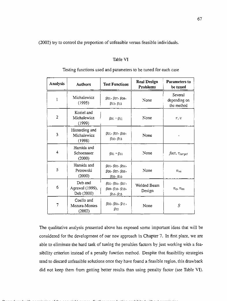
Reproduced with permission of the copyright owner. Further reproduction prohibited without permission.
67
(2002) try to control the proportion of unfeasible versus feasible individuals.
Table VI
Testing functions used and parameters to be tuned for each case
Analysis Au thors Test Fonctions Real Design Parameters to
Problems betuned
Michalewicz Severa!
1 go1, 90i· 9og, None depending on (1995) g1D· 913 the method
Koziel and 2 Michalewicz 901- g11 None r, v
(1999)
Hinterding and go1. 9oï, gog, 3 Michalewicz None -
(1998) g10, 913
Hamida and 4 Schoenauer 901 -911 None fact, /target
(2000)
Hamida and g01· 902· 904· 5 Petrowski go6, 90i· 908· None nm
(2000) gog, 910
Deb and go1· go4, 9oï. Welded Bearn 6 Agrawal ( 1999), gog, gw, g13· nc,nm Deb (2000) g14· 915
Design
Coello and 7 Mezura-Montes 902· 904, gu, None s
(2002) g12
The qualitative analysis presented above has exposed sorne important ideas that will be
considered for the development of our new approach in Chapter 7. In first place, we are
able to eliminate the hard task of tuning the penalties factors by just working with a fea
sibility criterion instead of a penalty function method. Despite that feasibility strategies
tend to discard unfeasible solutions once they have found a feasible region, this drawback
did not keep them from getting better results than using penalty factor (see Table VI).

Reproduced with permission of the copyright owner. Further reproduction prohibited without permission.
68
Another important observation is that the effectiveness of a GA was generally increased
when the algorithm tried to retain a good proportion of feasible and unfeasible individu
ais in order to produce a reasonable exploration of unfeasible regions. This may be very
effective when feasible regions in the whole search space are disjoint and far from each
other (Runarsson and Yao, 2000). Thus a possible path to tackle effective! y an optimiza
tion problem using GAs is by devising a computational method capable of compute such
a good proportion without neglecting the dynamic behavior of GAs and the application of
a feasibility criterion.
4.3 Adaptive Operator Techniques in GAs
The efficiency and effectiveness of Genetic Algorithms are highly determined by the de
gree of exploitation and exploration kept throughout the run. When the exploitation is
much higher than exploration the algorithm converge very rapidly and the solution is gen
erally a local optimal. On the contrary, when exploration is rouch higher than exploita
tion the algorithm converge very slowly and a lot of CPU time is necessary to reach a
global optimal solution. Several techniques have been proposed to control the exploita
tion/exploration relationship (EER) in order to avoid the premature convergence (Her
rera and Lozano, 1996; Arabas et al., 1994; Baker, 1985; Booker, 1987; Bramlette, 1991;
Davis, 1989; Fogarty, 1989; Rolland, 1992; Julstrom, 1995; Smith, 1993; Srinivas and
Patnaik, 1994a). Most of these works acknowledge the significant effect that GA control
parameters have over its performance.
There are two general forms of setting up parameter values: parameter tuning and param
eter control (Eiben et al., 1999). The first one is time consuming, even when parameters
are tuned one by one. In general, the selected parameter values are not necessarily opti
mal since parameters often interact in a complex way. Additionally, GA optimization is
in effect a dynamic adaptive process where at different stages of the evolutionary process
different optimal values of parameters might be necessary. For the second one, parameter

Reproduced with permission of the copyright owner. Further reproduction prohibited without permission.
69
control, different aspects of the evolutionary algorithms have been taken into considera
tion to classify them as it is indicated in (Angeline, 1995; Hinterding et al., 1997; Smith
and Fogarty, 1997; Eiben et al., 1999). Here, we will use the taxonomy presented by Eiben
et al. (1999) for its simp1icity and generality.
The taxonomy presented in Eiben et al. (1999) (see Figure 28) classifies the methods for
changing the value of a parameter into one of three categories: deterministic, adaptive and
self-adaptive.
Parameter setting
before the run during the run
Parameter tuning Parameter control
1 .... Deterministic Adaptive Self-adaptive
Figure 28 Global taxonomy of parameter setting in EAs
A method for changing the value of a parameter is deterministic when the value is altered
by sorne deterministic rule. In the case that the algorithm uses sorne form of feedback
from the search to establish the direction and/or magnitude of the change of the value,
the technique is adaptive. Finally, if the parameters to be adapted are encoded into the
chromosomes and undergo mutation and recombination then a self-adaptive technique is
being applied.
In (Davis, 1989), we can find one of the first efforts for adapting sorne GA's parameters.
The author adapts a global set of operator probabilities based on the performance of the
operators in the last generations (adaptation window lV). The performance of operators is
measured by the quality of the individuals they produce. Very recently created individuals

Reproduced with permission of the copyright owner. Further reproduction prohibited without permission.
70
are rewarded if their fitness is the best among ali other individuals in the population. The
size of this reward is determined by the amount of the improvement. Furthermore, a
certain percentage of the reward P is recursively passed on to the individual's ancestors
(to a certain maximum depth AI). This reward strategy is motivated by the fact that a
series of suboptimal solutions is often necessary in order to reach a better solution, and
that corresponding operators should th us be rewarded. With certain intervals I, the rewards
are used to update the probability setting. For each operator i:
, _ (l S) S rewardi P·- - p· -l.. 1 7 ' totalReward
(4.24)
where p~ is the new probability for operator i and S is the Shift factor. which determines
the degree of influence that the current update should have on the total probability setting
This algorithm requires a great deal of bookkeeping to sustain pointers only to living
individuals. Since the ancestral information is stored in the individuals, information is lost
when individuals die.
Rochenber's approach use feedback information on how well the search is going to adapt
the parameter control values (Thierens, 2002). He uses a rule to keep the ratio of successful
mutations to ali mutations close to ~. The step size of mutation is increased wh en the ratio
is larQ:er than L and it is decreased when the ratio is less than L ~ v v
The approach presented in Julstrom (1995) is very similar to the one in (Davis, 1989).
Here, the author uses a tree for each individual to specify which operators were used to
create its ancestors. Another difference is that rewards are assigned to individuals that
exceed the median individual instead of the best ones. Besides, when converting operator
rewards to a new probability setting, the author uses a greedy variant of the update rule
used by Davis (1989) (corresponding to S= 100% ). For each operator i:

Reproduced with permission of the copyright owner. Further reproduction prohibited without permission.
71
, rewardi Pi = -to_t_a-=-zR=--ew_a_r_d (4.25)
where p~ is the new probability for operator i.
In (Whitley, 1989), the authors use Hamming distance between the two parents during re
production to measure genetic diversity. The more similar the two parents, the more likely
that the mutation operator would be applied to bits in the offspring created by crossover.
Wilson's approach (Herrera and Lozano, 1996) uses the entropy over the population to
adjust crossover probability. When entropy is falling then Pc is adjusted up slightly, ether
wise, is adjusted down.
In (Li et al., 1992), the authors use two diversity functions for describing GA behavior and
controlling the Pc and Pm parameters. The function BC measures the diversity between
chromosomes in the population and control the changes in Pc; the other function BA
measures the diversity between the alleles in all the chromosomes and control the changes
in Pm· They divided the whole optimization process in three stages: initiation, search and
refinement. They consider that each stage should have different degree of exploitation and
exploration. So, for each stage BC and BA has different maximum and minimum critical
limits.
In (Srinivas and Patnaik, 1994b), the authors adapt the probabilities of crossover and mu
tation CPc and Pm). Besides, each chromosome has its own Pc and Pm· Both parameters are
computed by using:
{ kl(fmax- J')/(fmax- J), J'~ J
Pc= k J'< -J 3, (4.26)
and

Reproduced with permission of the copyright owner. Further reproduction prohibited without permission.
72
(4.27)
where f is the chromosome's fitness, ]best is the population maximum fitness, 7 is the
mean fitness, and kb k2, k3 and k4 are constants ~ 1.0. This algorithm increases Pc and
Pm when the population tends to get stuck at a local optimum and decreases them when
the population is scattered in the solution space.
Herrera and Lozano ( 1996) use fuzzy logic-based tools for controlling GAs by incorpo
rating human expertise and knowledge. The main idea here is performance measures of
the GA are sent to a fuzzy logic controller (FLC) which computes new control parame
ters values that will be used by GA in the next generation. The authors use two diversity
measures GD and PD as inputs. The first one is a genotypic diversity measure based on
Euclidean distances of the chromosomes in the population from the best one. The other is
a phenotypic diversity measure based on the fitness.
Munteanu et al. ( 1998) propose an adaptive method for choosing the mutation and crossover
rates. They use the maximum desired or expecteà value of fitness Fmax and the stan
dard deviation of fitness in population .stdi (!) to compute the probability of mutation and
crossover in each generation by using:
p(i+l) = { p(i) + C log ( Fmax e-stdi(f)) . \fi m m 1 F~L, . (4.28)
(4.29)
where pr;J and p~i) are the probability of mutation and crossover in generation i respec
tively, F~~x is the best fitness up to generation i, and C1 > 1 and C2 > Fmax are constants

Reproduced with permission of the copyright owner. Further reproduction prohibited without permission.
73
which values depend on the specifie problem.
Gong et al. (2002) use the relation between diversity of evolution population and evolution
times to control the number of crossover and mutation operations points. To compute the
diversity of evolution population, they compute the following function:
F(t) = 1- H(t) L
(4.30)
where H(t) is the hamming distance among the individuals genes, t is a variable of the
current generation, and L is the length of individual coding. This population diversity
function F(t) is decreased by a factor p(t) defined as:
-t2 p(t) =exp( 2a2) (4.31)
where a = T /3 and T is the maximum number of generations for the optimization process.
The authors set up a group of decision intervals for the value of F(t)p(t) in order to set
the number of crossover and mutation operation points.
Table VII summarizes sorne characteristics of the adaptive techniques reported above. The
second column (Oper.) refers to the operator or parameter that the technique has tried to
control. We can see that all articles but one have tried to control the mutation probability.
However, the last publications report that the adaptive techniques have targeted not only
the mutation but also the crossover probability. The column "Measures" indicates the type
of information obtained from the optimization process of the GA that the technique has
used in order to do the adaptation. Here, it is clear to see that there is not a standard
measurement method. The column "Strategy" summarizes the way the adaptive technique
changes the probability values. The column "Param." shows us how sorne methods use
more parameters which means that the complexity has increased. In fact, as the number of
parameters is increased, it is more difficult to know which set of parameters is optimal to

Reproduced with permission of the copyright owner. Further reproduction prohibited without permission.
74
work and whether it will work efficiently with other type of problems. A very interesting
idea is presented in the column "Observation" which cornes from Li et al. (1992). The au
thors realizes that there are different stages along the optimization process where diversity
is different from one stage to another.
The analysis presented above uncovers sorne interesting ideas that are used in Chapters 7
and 8. For the design of any adaptive technique, we should consider that the optimization
process of GA goes through different stages which suggest different strategies for adapting
Pm and Pc· It seems that it is easier to control or to adapt Pm than Pc· It is also important
to highlight that besides that there is not a standard way to measure diversity neither there
is an analysis of how the existing indexes work with different types of mutation operators
or crossover operators. Neither there is a report of using Bayes Network for controlling Pc
and pm.

Reproduced with permission of the copyright owner. Further reproduction prohibited without permission.
75
Table VII
Summary of Adaptive Techniques
Au thor Op er. Measure Strategy Param. Enc. Observation
Thierens Ratio of Change step Keep the
(2002) Mutation successful size of None B ratio arround
(Rechenberg's mutation mutation 1
approach) 5
Davis (1989) Severals Quality of
Reward W,P,S,I,
B Pass reward
individuals M to ancestors
Julstrom Quality of "\IF,
Pass reward ( 1995)
Severals individuals
Reward DECA.Y, -I,DEPTH to ancestors
Herrera and Lozano ( 1 996)
Crossover Entropy Change Pc None B (Wilson's
-
approach)
Whitley Mutation
Hamming Cali None B
(1989) distance mutation -
Decision
Mutation Two ru les Assume three
Li et al. (1992) and diversity according to
BC,BA. B stages for the
Crossover functions: values of optimization
BC and BA. BCand process BA
Srinivas and Mutation Each
Patnaik and Fitness Compute kl. k2. k3. B
individual
(1994b) Crossover Pm and pc k4 has its own
Pc and pm
Two Fuzzy
Herrera and Mutation
diversity Logic
Lozano (1996) and
functions: Controllers None R -
Crossover compute the
1
GD and PD new values
Munteanu Mutation
Statistic Compute et al. ( 1998)
and information Pm and pc
c1.o2 B -Crossover
Gong et al. Mutation
Hamming Rules for (2002)
and distance intervals
F(t), p(t) B -Crossover

Reproduced with permission of the copyright owner. Further reproduction prohibited without permission.
CHAPTER5
METHODOLOGY AND GA
This chapter presents, first, the methodology that has been applied along ali our research.
We then explain the study of different architectures of GA in order to arrive to one basic
configuration, the one that will be modified in the next chapters.
5.1 Methodology
It is important to emphasize that for the design of GAs, flexibility is essential, and only
in sorne occasions results do match preconceived hypotheses. New and improved GAs
are frequently published, with the driving motivation of being novelty; however, in many
cases, previously introduced GAs are simpler, and have identical or better performance.
Research in the GAs domain has been dominated by two opposite types of approaches, ad
hoc experimentation and looking for a precise mathematical modeling of GAs. Finding
exact models of GAs has resulted in a more complex and analytical unwieldy task than
the GAs themselves, and only in very few occasions has resulted in improved designs for
GAs. Much ofthe difficulty lies in the fact that GAs are complex systems, and successfully
modifying the design of a complex system is an involved, multifaceted undertaking. What
is often needed is an approach that combines intuition, coarse analysis, and thoughtful
experimentation.
The methodology used along ali our research aims to answer the following issues related
with the analysis, design and testing of our GA:
1. Should we use C language, C++ language or matlab script language for coding?
2. Should we start working on a non-commercial application of GAs or should we
program our own GAs?
3. Where on the GA architecture should we work in order to improve its performance?

Reproduced with permission of the copyright owner. Further reproduction prohibited without permission.
77
4. What kind of testing should we do to initially test our implementation of GAs and
to compare the results of our proposed solutions with ether works from ether re
searchers?
5. What kind of measurement indexes should we use to evaluate the performance of
our GAs for all the tests including the business jet problem?
6. Which cases from the flight envelope of the business jet problem should we use as
testing problems?
First, several reasons supported our decision to use Matlab script language in implement
ing our GAs. Among these, it was key that Matlab has become a de-facto standard in
Computer Aided Control System Design (CACSD), and when we started our research the
simulation mode! of Bombardier had been previously translated from Xmatrix to Matlab
by the team of ETS-Bombardier project. It also provides a wide range of toolboxes, no
tably the Control System, Neural Network, and Optimization Toolboxes, and the Simulink
non-linear simulation package along with extensive visualization and analysis tools. Mat
lab has an open and extensible architecture allowing individual users to develop further
routines for their own applications. These qualities provide a uniform and familiar envi
ronment on which to build genetic and evolutionary algorithm tools. In addition, Matlab
script language presents several advantages over the ether choices; fas ter for writing a pro
totype, easier for maintenance and testing, easier to integrate with the simulation mode! of
Bombardier, and also includes a way to generate C or C++ code from Matlab functions.
We tried at the beginning (Garda et al., 200 l) to use C language to implement our GA and
to interface it with the simulation model; we experienced sorne difficulties due to the inter
action of Matlab script with a different language. In our case, the benefits (fast execution)
gained from using C or C++ language is worthless because the time of execution of the
simulation mode! is in fact our bottleneck. and not the performance of the implemented
code of the GA.

Reproduced with permission of the copyright owner. Further reproduction prohibited without permission.
78
Second, we chose to develop our own GA software despite the existence of non-commercial
applications. The advantage of this approach was the ftexibility of adding new methods
following our line of investigation. Besides, as we found in the literature review, there
is not a standard architecture of GA to solve any type of problem. However, we have
used one non-commercial implementation of GA and another of Evolution Strategies for
general comparison, specially when new methods proposed in this thesis have been im
plemented.
To decide the kind of strategy to follow in order to improve the performance of GAs,
Pham and Karaboga (2000) remind us that in genetic algorithms, factors like the encod
ing method, the scheme to generate the initial population, the evaluation function, and the
genetic operators are problem dependent, while a fifth factor, setting up GA control pa
rameters, tends to be much less problem dependent, allowing much more scope for generic
work in order to control the degree of exploitation and exploration of the algorithm and
by this means to improve its performance. Therefore, we decided to fix the three first fac
tors and to work on the fourth and fifth factors. Though working on the genetic operators
is problem dependent, there exist multiple possibilities of implementations by fixing the
encoding mechanism to real values, so we kept our strategy flexible enough to reach our
goals.
For the testing stage, we followed a two step testing process which includes. first, to solve
two sets of mathematical functions commonly used in the genetic algorithm literature
(Michalewicz, 1996), one for unconstrained global optimization (see Appendix 1) and
another for constrained global optimization (see Appendix 2), and second, to solve a set
of cases from the business jet's ftight envel ope.
The literature contains a variety of criteria for evaluating heuristic methods like GAs. Ac
cording to Barr et al. ( 1995), in a well-rounded study of performance measures, three
dimensions are important: solution quality, computational effort, and robustness. To mea-

Reproduced with permission of the copyright owner. Further reproduction prohibited without permission.
79
sure the quality of the solutions in our experiments we recorded the speed and rate of
convergence to the optimal solution, as well as the percent of deviation from the best op
timal. For the computational effort, the number of generations required to find and report
the solution, the number of function evaluations and the total run time were the measure
indexes selected. We addressed the robustness of our proposed improvements in GAs by
testing and measuring the variability of their performance in a set of mathematical test
problems as well as in a sampling set of cases of practical application.
While the ftight control envelope of Bombardier's problem includes 160 points of op
erations, we exclusively analyzed the application of GAs in a set that was also used in
(Boukhari, 2002). However the best results for the 160 points are presented in Appendix 5.
The development of our software followed an iterative approach of analysis, design, cod
ing, and testing. The following sections present previous work done in order to arrive to a
basic architecture before any new improvements.
5.2 Getting the best architecture for departure
Before proceeding with any ki nd of improvement or important changes, we needed to start
with a simple architecture of GAs. We analyzed each component of GA architecture and
selected its part by using the GA literature available, or, also by repeated testing.
5.2.1 Encoding Mechanism
Several studies support the use of ftoating-point representation in real parameter problems
instead of the binary one. Goldberg (1990) gives the following reasons:
a. no need of transformation between genotype and phenotype because of one-gene
one-variable correspondence~
b. avoidance of Ham ming cliffs;

Reproduced with permission of the copyright owner. Further reproduction prohibited without permission.
80
c. fewer generations to population conformity.
Results from Janikow and Michalewicz (1991) also indicate that GAs using fl.oating point
representation are faster than binary GAs, more consistent from run to run, and provides
higher precision (especially with large demains). They also added that the performance
of using fl.oating-point encoding can be enhanced by special operators to achieve high
accuracy. For Davis (1989), real coding allows domain knowledge associated with real
world domain to be easily integrated into the RGAs for the case of problems with non
trivial restrictions.
5.2.2 Reproduction operators
Although crossover and mutation are the reproduction operators used most frequently in
GAs, crossover has always been regarded as the primary search operator because it ex
ploits the available information from the population about the search space (Herrera et al.,
2003). The main research effort on RGAs has been spent on developing efficient crossover
operators, and as a result many different instances have been proposed (see (Herrera et al.,
1998) for more detail).
Herrera et al. (2003) proposed a taxonomy that groups the models for this operator in dif
ferent categories according to the features associated with the offspring generation mech
anism applied on the genes of the parents (Figure 29).
TYPES OF CROSSOVER
Discrete Aggregation-based N eighborhood-based Hybrid
Figure 29 Taxonomy of crossover operator for RGAs

Reproduced with permission of the copyright owner. Further reproduction prohibited without permission.
81
There are four groups in this classification: the first one is the discrete crossover operators
(DCOs) that includes th ose that are presented for binary coding and are directly applicable
to real coding. They generate a corner of the hypercube defined by the component of the
two parents.
The second one is the aggregation-based crossover operators (ABCOs) that includes those
operators that use an aggregation function that numerically combine the value of the genes
of the parents to generate the value of the genes of the offspring in the exploitation interval
or in the exploration interval. An example of this group is the arithmetical crossover.
The third group named neighborhood-based crossover operators (NBCOs) includes cross
avers that apply probability distributions to the intervals defined by neighborhoods asso
ciated with the genes of the parents in order to determine the genes of the offspring. In
general this type of operators generates genes in relaxed exploitation intervals. Exam
ples of NBCOs are BLX - a: and SBX, which are based on unifonn and exponential
probability distributions, respectively.
The last group is called hybrid crossover operator (HCOs) and it includes those operators
that apply offspring generation mechanism from different categories. In this way, these
operators obtain different levels of exploitation and exploration along the search process.
According to the empirical results of Herrera et al. (2003), the best crossovers are the
NBCOs that build the offspring through relaxed exploitation intervals. Among them we
have selected the simplest one in implementation, BLX - a:, for our initial GA architec
ture. This operator has been reported to perfonn very well with a: = 0.5 (Deb, 2003, page
9). ln a previous work of Herrera et al. (1998), they show that as a grows and the relaxed
exploitation zones spread over exploration zones the diversity levels increase too allowing
good zones to be reached. Their results also show that at a: = 0.5 it is possible to induce
an efficient exploration and exploitation relationship.

Reproduced with permission of the copyright owner. Further reproduction prohibited without permission.
82
For selecting the mutation operator we used the empirical analysis done by (Janikow and
Michalewicz, 1991; Michalewicz, 1996; Herrera et al., 1998) where they compare the
nonuniform mutation operator against ethers. The nonuniform operator presents good
results specially as the search process advances where the operator starts to reduce the
genes generation interval in smaller zones around the gene to be mutated and start to
produce a local tuning on the solutions. The zones close to the best found solution are
visited, which may be considered good enough for believing that the optimal solution is
close to them.
5.2.3 Selection operator
During the evolution process of the genetic search, two important issues are strongly re
lated: population diversity and selective pressure. The main problem here is the inverse
relation between these two factors (Whitley, 1989). Hard selection concentrates on the
exploitation of information gained so far and produces a high convergence speed. On
the ether hand, soft selection tries to keep genotypic diversity and does more explorative
search, leading to good convergence reliability but Iow convergence speed.
Severa! methods have been suggested to quantify the effect of the selection pressure that
selection operators exert on the population. Th us, Goldberg and Deb (1991) defi ne the
takeover time, which is the number of generations that the selection algorithm takes to
reproduce a single representative of the optimal solution to occupy the entire population.
Using this term short takeover times are synonym of high selection pressures. Another
way to quantify the selection pressure is using the definition of selection intensity, a con
cept original from the field of quantitative genetics (Thierens, 1997, see page 153) and
introduced into the evolutionary computation domain by Muhlenbein and Schlierkamp
Voosen (1993). Selection intensity is defined as the increase of the mean fitness of the
population after selection normalized by the standard deviation. A high selection intensity
corresponds to high selection pressure. While takeover time or selection intensity may

Reproduced with permission of the copyright owner. Further reproduction prohibited without permission.
83
quantify in sorne way the effect of the selection pressure they may not be sufficiently com
plete representations; therefore, more sophisticated models of selection that consider the
cumulative of the fitness distribution have been suggested by Rogers and Prügel-Bennett
( 1997); Blickle and Thiele ( 1996); Cantu-Paz (2002).
Table VIII
Studies on Selection Methods
Reference Type of Study Criteria Selection
Conclusion Methods
(Goldberg Growth ratios, Pro porri onate, Linear Ranking
Only consider the Ranking, and Binary and Deb,
effect of selection takeover ti me and
Tournament, Tournament 1991) time complexity
Genitor Selection
Theoretical and Fitness
Tournament, (Blickle and
experiment with distribution.
Truncation, Tournament Thiele, 1995) selection
Onemax function intensity
Ranking
Solution quality Proportional,
(Zhang and Real-life problem and convergence
Ranking. Ranking, Kim, 2000) Tournament, Tournament
ti me Genitor
Linear Ranking,
Theoretical and Exponential
(Cantu-Paz, experiment with
Fitness Ranking, Boltzmann
2002) distribution Boltzmann, Onemax function
Truncation, Tournament
Although sorne studies like the ones shown in Table VIII have compared the selection
methods most frequently used in genetic algorithms, and have arrived to sorne important
conclusions, Camu-Paz (2002) emphasizes that there is no single best selection method.
Thus, it is quite possible that a selection method that works weil in combination with
certain operators on a particular problem may have a poor performance in a different
setting. So we decided to try the linear ranking and binary tournament selection that are
reported with the best performance in Table VIII and test them in our problem with the
rest of settings.

Reproduced with permission of the copyright owner. Further reproduction prohibited without permission.
84
We also decided to use the elitist scheme by replacing al ways the worst individual of the
next generation with the optimal one currently available. This assures us that the optimal
solution once found is never lost unless even better solution is created.
5.3 Tests
The goal of these tests was to select a base configuration of GA which could be easily
modified in order to improve its performance and to be applied effectively and efficiently
to the optimization of controller gains of a fly-by-wire system. So far, we have explained
how mutation and crossover operators were chosen for our architecture, but we have not
yet identified our selection operator. To do so, we did two types of experiments: the first
one with the set of mathematical functions and the second one with the practical cases.
Besides the linear ranking selection and tournament selection schemes, we also tested a
geometrie selection scheme (Michalewicz, 1996). The reason was that there were few
studies about this scheme and we found in a sampling test that it performed better than the
linear ranking. Table IX shows the three GAs'configurations tested.
Table IX
Test configurations of GAs
Name Crossover Mutation Selection RGA-1
Nonuniform Linear Ranking (1Jmax = 1.1)
RGA-2 BLX -0.5 (b = 5)
Geometrie (q = 0.08) RGA-3 Binary Toumament
We selected as the basic configuration of GAs the one that in most of the test functions
and business jet's cases obtained the smallest standard deviation and mean, and the closest
one to the true optimal.
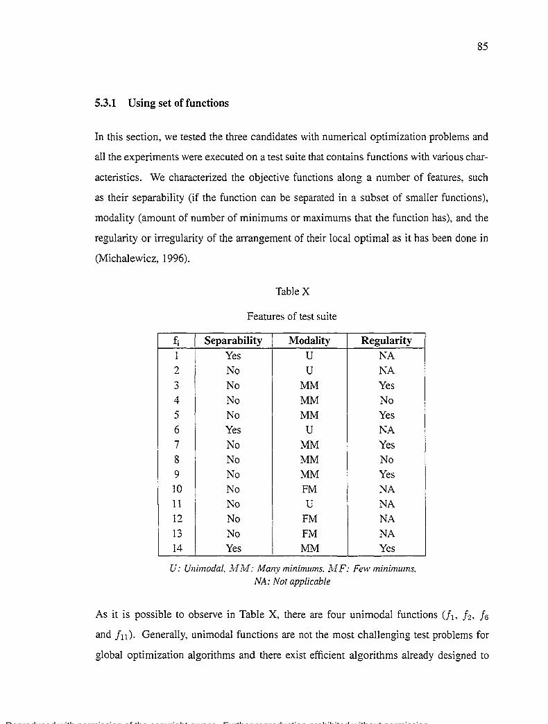
Reproduced with permission of the copyright owner. Further reproduction prohibited without permission.
85
5.3.1 Using set of fonctions
In this section, we tested the three candidates with numerical optimization problems and
ali the experiments were executed on a test suite that contains functions with various char
acteristics. We characterized the objective functions along a number of features, such
as their separability (if the function can be separated in a subset of smaller functions),
modality (amount of number of minimums or maximums that the function has), and the
regularity or irregularity of the arrangement of their local optimal as it has been done in
(Michalewicz, 1996).
Table X
Features of test suite
f. 1 Separability Modality Regularity
1 Y es u NA
2 No u NA "' No MM Y es .)
4 No MM No
5 No MM Y es
6 Y es u NA
7 No MM Y es
8 No MM No
9 No MM Y es
10 No FM NA
11 No u NA
12 No FM NA
13 No FM NA 14 Y es MM Y es
U: Unimodal, 1\1J\Il: Many minimums, A1F: Few minimums, NA: Not applicable
As it is possible to observe in Table X, there are four unimodal functions (j1, f2, f 6
and f 11). Generally, unimodal functions are not the most challenging test problems for
global optimization algorithms and there exist efficient algorithms already designed to

Reproduced with permission of the copyright owner. Further reproduction prohibited without permission.
86
solve them. However, their inclusion in the set is to use them to get an idea of the con
vergence rate of the new changes that we propose in the next chapters. There are also ten
multimodal functions, seven of them (]3, f4, Jo, fï, f 8 , fg and fv.) have a number of local
minima that increases exponentially with the function dimensions, while the other three
Cf1o, !r2 and j13) have only a few local minima. The use of multimodal functions is to fi nd
if whether an algorithm can have a better mean and standard deviation, as weil as better
solution in a shorter time.
Although there may exist sorne relations among the behavior of the reproduction opera
tors and the selection scheme, we decided to use the same value of parameters for ali three
configurations. This means that we were trying to find the best of the three configurations
given the same set of parameters, crossover and mutation operators. Table XI summa
rizes the dimensions of each test function, the population size for the GA as weil as the
maximum number of generations for the stop criteria, the probability of crossover and the
probability of mutation.
We ran 50 iterations for each function and we recorded the minimum cost, the maximum
cost, the mean cost and the standard deviation of the 50 iterations in Table XXX to Ta
ble XXXV of Appendix 3.
To visualize in a better way which of the three configurations was the most convenient to
choose, Figures 30, 31, and 32 report the position that was assigned to each algorithm as
a result of getting the best values. In the case when two or ail of them got the same value
they were also granted the same position. The ad van tage of this approach is that it is easy
to observe which one presented the best results.
Figure 30 shows clearly that RGA-2 was able to obtain the best optimal values for the
whole set of functions. However, Figures 31 and 32 say that the RGA-3 got the smallest
mean and standard deviation most of the ti me, and it was good enough in returning optimal
results.

Reproduced with permission of the copyright owner. Further reproduction prohibited without permission.
Tahle XI
Parameter settings of GAs
fi Numberof Population Numberof Variables Size Generations Pc
1 20 40 2000 2 5 40 5000 3 40 5000 4 20 5000 5 10 40 5000 6 20 2000 7 40 5000 0.95 8
5 40 5000
9 20 2000 10 20 2000 11 2 20 2000 12 20 2000 13 20 2000 14 20 40 5000
4r-~------r-----~-----r----~~----~----~
........... :•~,.-.-:-+-'-· """R-G-A--1-.J
1 - RGA-2 1 -o- RGA-3
1 ' 1 •
1 ' . . .. . . . . ' ............ . 1
1
1
. ' ' : ·.
1
1
1
1
1
... ····•·. 1
1
1
1
1
Pm
0.05
0~~2------4~----~6------8~----~10~----~12~--~14
Figure 30 Position according to the results of optimal cost
'f.7

Reproduced with permission of the copyright owner. Further reproduction prohibited without permission.
= 0
~
4r---?-------~-------r-------,--------r-------?-------,
·····~-·-ô-·-·•····· • • ~
~
-,r;r·-~<\·:-·· : '" : . ·~
·+ RGA-1 ~ RGA-2 --- RGA-3
········-:--~···~~·····-=······
, : ~
1 :
1
• ' ' . ·Q··, ... c •....
' -' ~ . '" : 'i: ,_: ,_: t'
• • •
..........•..
o~---&2--------~4--------~6~--------s~--------~~o~------~~2~------~14 r,
Figure 31 Position according to the results of average cost
4r---?-------~-------r-------,--------r-------y-------,
·+ RGA-1 ~ RGA-2 -e- RGA-3
• • .. .... ...•..
oL---~------~--------~-------L--------~------~------~ 2 4 6 8 10 12 14 r,
Figure 32 Position according to the results of standard deviation of cost

Reproduced with permission of the copyright owner. Further reproduction prohibited without permission.
89
The two-dirnension fonctions ]!0- f13, as well as f 6 and h were very easy to be solved by
ali three configurations; and among the unimodal functions the only difficult one was f2
where its global optimum is inside a long, narrow, parabolic shaped fiat valley. From these
findings we were able to discard the linear ranking configuration RGA-1. Then, since the
aim of this thesis is to apply GAs to real problems using few evaluation fonctions (short
time ), we decided to reduce the maximum number of generations of execution by half
of the current value during three occasions. As the number of generations was reduced
we also increased Pm by 0.05 of its current value in order to facilitate the exploration of
RGA-2 and RGA-3.
-4.54
-4.56
-4.58
-4.6
c -4.62
"" -4.64
-4.66
-4.68
-4.7
0··· :•
0.125
Gcner».tion ratio
Figure 33 Mean cost using fonction fg
~- RGA-31 ~·· RGA-2
8oth configurations presented significant changes in their mean and standard deviation
when they tried to optimize fonctions f2, !3, f 4 , f 8 , f 9 and fi 4 (see Appendix 3). Though
there were significant changes, in sorne cases RGA-2 outperfonned RGA-3 (see Fig
ures 35 and 36) and in others it was the contrary (see Figures 33 and 34), it was not
possible to discriminate which one was the best wh en the number of maximum genera
tions was reduced. However, it was clear that RGA-3 became slightly better than RGA-2

Reproduced with permission of the copyright owner. Further reproduction prohibited without permission.
when the interval of generations for the optimization process was large enough .
c 0 =
0.08 . . . . . . . . . . . " .1-:. ~~=~ l. 0.07
0.06
-E 0.05 -= 'E ] 0.04
<;;
c
0.03
0.02
0.01 .,.
0~0~.1~25~----0~.~25~------------~0~.5~--------------------------~~~ Gc:neradon rado
Figure 34 Standard deviation of results using function f 9
-1510~~----~~------------~~------------------------------,
Q -1530 ......
......... 1:::- ~~=~ 1. . ··········
~ -1540 :;.
'· '· -1550 .. ..................... ~,
-1560 '· '· . -a:..:::.:.·.::·.:.··.:.. - - - - -·- - - -·
-1570~o.~1~25~--~o~.2~5~------------o~.~5-------------------------------J G~neratfon rado
Figure 35 Mean cost using function j 14
90

Reproduced with permission of the copyright owner. Further reproduction prohibited without permission.
30
~ 25 ·~· ........ .
"; "E "" 20 ~ ] t;; 15
10
5
0 0.125
. ·:···· ., ... "· ...
" ············· ....
0.25
......... !~ ~~=~! ...... ..
.... . .. . .... : ·-···········-···.-.·.·~····· ............ .
..................... ,..., . ._. ....... . ·-0.5
Generation ratio
Figure 36 Standard deviation ofresults using function ]I4
5.3.2 Using practical ftight cases
91
The test suite functions allowed us to eliminate the RGA-1 choice, so now in this section
we used the flight cases available tous to evaluate the perfonnance ofRGA-2 and RGA-
3. The parameters for both configurations were a population size of 20 individuals or
chromosomes, a Pm = 0.20 and a Pc = 0.95.
Although the differences in the average cost between RGA-2 and RGA-3 (Figure 37) was
very small for ali eight cases, RGA-3 was able to perform better in seven of them. The
standard deviation of the results in the simulations showed us that RGA-3 achieved values
of standard deviation less than 0.005 for seven ofthe eight cases while RGA-2 was able
of similar perfonnance for only five cases. Therefore, RGA-3 is selected as the base
algorithm to be used along the next chapters.
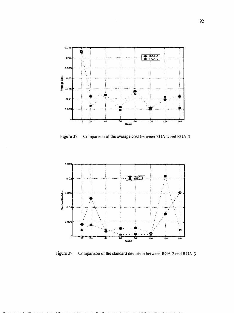
Reproduced with permission of the copyright owner. Further reproduction prohibited without permission.
o.~r---~--,-----~~----~------r-----~------~----~-,
0.03 ..
0.025 ...
~ 0.02 .. u ..
~ \\ ·:··_!'' : ,\
:! '. \ : l 0.015 ..... ; .... ~.,,.; ..... .. ---. 0.01 ....
Ill 0.005 .....
1* RGA-31 . -a- RGA-2
. . ' . ~ ... ·-· ............ .
• . ................ . ...... :e< .... . ......•. oL----1~2~~2~4~-----44~------64~------~84~----~1~04~----~1~2~4----~1~44~
Case
Figure 37 Comparison of the average cost between RGA-2 and RGA-3
0.025r----r----~------,-------,--------r------~------~------~--,
0.02 .....
c: ~ 0.015
~ 0
] .., c: s
<1) 0.01
0.005 ..
0
., 1: \
-- /.L -~\ 1 \
1
1
1
• • 12 24 44 64
1
• RGA-3j ; . -11- RGA-2 t·· .. ; ·
.. ,
1 ... , ..
84 104 Case
Il --,:'········· ,:' 1:\
. \. .
" , 1
,
••• ; •• ·'·. ,1,. 1 1
124
•• '·
1. 1
1·
144
Figure 38 Comparison of the standard deviation between RGA-2 and RGA-3
92

Reproduced with permission of the copyright owner. Further reproduction prohibited without permission.
CHAPTER6
PERIODIC MUTATION OPERATOR
As mentioned in Pham and Karaboga (2000), setting up GA control parameters tends to be
rouch less problem dependent, allowing more scope for generic work in order to control
the degree of exploitation and exploration of the algorithms and by this means to improve
its performance. We have to keep in mind that our goals are to reduce the number of
function evaluations (reduce ti me of execution) and to reduce the standard deviation of the
cost function in such a way that indistinct} y of the business jet's case we can increase the
likelihood that our GA gets a result very close to the global optimal in the first run.
Even though the control of one or few parameters related to a single operator of GA is
not difficult, there has not been any report of the application of parameter control tech
niques in GAs applied to aircraft controller design problem. This chapter presents a new
mutation operator that tackles the second and third of our goals. To implement our new
operator we decide to use a deterministic control scheme on Pm (mutation probability) and
in order to understand the way this new operator works we briefly examine the strengths
and weakness of uniform and nonuniform mutation operators (Michalewicz, 1996). Then,
we explain how our proposed scheme works and give next the results of severa} tests and
their analysis.
6.1 Uniform Mutation Operator
The uniform mutation operator is similar to the classical version ofbinary encoding, where
each element xk of a chromosome x= (x1: x 2 , ···: Xk, ... , Xn) has exactly equal chance of
being mutated and the result x~ is a random value from its corresponding domaink. While
having a constant uniforrn mutation probability allows GAs to explore the search space,
this scheme do es not have a high impact in the degree of exploitation do ne most of the ti me
by the crossover operator; therefore, it is very likely to expect, in short periods of execution

Reproduced with permission of the copyright owner. Further reproduction prohibited without permission.
94
(small number of generations), a very low effectiveness (high standard deviation) of the
GA. This means that we should run several times the algorithm to make sure that we have
a good optimal solution.
6.2 Nonuniform Mutation Operator
Schemes similar to th ose used in (Hesser and Manner, 1991 ), (Janikow and Michalewicz,
1991) and (Back and Schütz, 1996) where the probability distribution of mutation is not
uniform and decreases over ti me favoring the exploitation of local solutions at 1ater stages,
increase the effectiveness (lower standard deviation) of GA specially for long periods of
execution (large number of generations). In other words, we should run the GA once but
using a large number of generations and get a very good solution.
6.3 Periodic Control Scheme
To implement our new operator, we decided to use a deterministic control scheme on Pm
(probability of mutation). The idea behind our proposed scheme is to use a strategy be
tween the two schemes described above in order to meet the conditions of our practical
application. Thus, our new operator should follow a scheme that decreases its value of
probability over time in order to favor the work of the crossover operator; however, be
cause the time of execution is short then it is necessary to have the possibility of doing a
last stage of exploration during the last generations to diminish the probability of miss
ing a better global optimal, and this may be possible by slowly increasing Pm· Although
there exist many schemes that cou1d follow the suggestions described above we chose a
simple one like a sinus function with a period greater than the maximum number of gen
erations, that start on the first high top, it does not have negative values and it has to be
less than or equal to one; the last two conditions mean that we have to add one and di vide
by two. Moreover, our new operator should have a uniform distribution for the mutation
probability, to facilitate the exploration.

Reproduced with permission of the copyright owner. Further reproduction prohibited without permission.
95
For the implementation of the proposed operator, we modified the relation presented ini
tially by Janikow and Michalewicz (1991). In their approach, one variable k is selected
randomly, and its value is set to a random number following the expression (6.1 ):
xt+l = { x~+ .6.(t~ u(k) - xk) if r < 0.5~ k x~ - .6. ( t, x k - l ( k) ) if r > 0. 5,
where
r represents a uniform random number between (0~ 1),
t is the current generation,
T is the maximum number of generations,
b is a shape parameter, and
u(k), l(k) are the upper and lower borders of x k.
(6.1)
(6.2)
For the periodic mutation operator, we propose to use the following expression instead:
where
and
yr ( (27i(t +a))) .6.(t, y)= 2 1 +sin Tp
5 T, = -T
p 4
Tp a=- -12.5
4
(6.3)
(6.4)
(6.5)
Both expressions, (6.2) and (6.3), use high mutation values at the beginning of the search,
allowing the operator to explore different regions of the search space during sorne genera-

Reproduced with permission of the copyright owner. Further reproduction prohibited without permission.
96
ti ons, and reduce later the degree of exploration (degree of mutation) to facilitate the work
of the crossover operator in the exploitation of the regions around the best individuals.
While the method suggested in (Janikow and Michalewicz, 1991) does not allow further
increment of the mutation rate, the expression proposed in this research permits a second
and final exploration of new regions (Figure 39).
2~--~---,----~---r---,----~---r--~~--,----,
ar:·:·:-:-:·· ... _; ......... ~ .......... ; .......... : .......... : a : ;·... : : . :
........ .- ....... . 1.8
1.6 ....... -~. -~- .. : .=~~· ..... <.· -~· ......... ; .......... : ......... ·> ..
. .. . 1.4 .. as·· .. ····;·F·····r<_·······~········r·······r·······
.... ~ ......... ~ .•.. a. ... :. .. • ........ :. ......•.. : ......... :. · a : a·. : : · 1.2 : : a: ·. : : :
~ 1 --~·-·--~----~--~à''~---·~···-~~--.. -~·········~·-······~ <f a . . . ·.: . . -~
a : : .:-
0.8 ···a···-~··· • · · · --~ · · · • · · · · -~ · · · ··· ·· .:-.. · · · · · · .;. · ·· · · · ·· .:. · ·· · · · · ~- · · ·· .. ·": . a : •• . .
a : a : : 4 ~ ··.. .ti a
::: à ~al a:~>-:~ .f_, ... : ~:. ·j ... ~ ·:·~~~~-: ~ -~·;.r_:::.::: .[..... . .... ::: :_.:.:.?~: ;: . . · ~a a
o.2 % · .. raa ....... ~: .. ~~---~-:-à"··;.·:··:,a~~~a·=.:a· . .:······ : .. ;,".: : ;J.•' a~ ~ra: ·a ·a. :a a " : a : a : aH '!tet!.~ ~·
0oL---~2o~~~4o----s•o--~s~o---1~o~o~~1~2o~--,4~0.c~16~o~-1~8~0--~2oo Generation Number (t)
Figure 39 Periodic variation of mutation
6.4 Tests
Again we divided our tests in two groups, one with the set of mathematical functions and
the ether with the practical fl.ight cases. Although, the tests were performed with the who le
set, here, we only present the results obtained using the most relevant of them, !3, f 4 and
fr4, which were also the hardest for optimization in chapter 3. With the mathematical
functions, we perfonned two types of sub-tests: in the first one, we used two different sets
of probability values for Pm and Pc, and, in the second one, we used two different selection
strategies. The objective of these two kind of tests was to observe the behavior of the
periodic mutation operator with those changes.

Reproduced with permission of the copyright owner. Further reproduction prohibited without permission.
97
Thus, besides the two configurations RGA-2 and RGA-3 used in chapter 3 we tested two
new ones, RGA-4 and RGA-5 (Table XII).
Table XII
Test configurations of GAs
Name Crossover Mutation Selection RGA-2 Nonuniform Geometrie (q = 0.08) RGA-3
BLX -0.5 (b = 5) Binary Tournament
RGA-4 Periodic
Geometrie (q = 0.08) RGA-5 Binary Tournament
6.4.1 Using set of functions
For the optimization of mathematical functions we used RGA-3, RGA-4 and RGA-5 con
figurations. We measured the average cost and the standard deviation of the results pro
duced by 50 runs of each configuration using different number of generations as stop crite
ria. We started using 100 generations and then we incremented by 50 unti1 we reached 550
generations. The objective with this variation of stop criteria was to observe the perfor
mance of the configurations as the number of function evaluations was increased. Ali the
tests were initially performed in a PC with a pentium III 733MHz, and 0.5 Gb of RAM.
Wh ile similar results were obtained by tes ting the mathematical functions with 5, 10 and
20 variables, we present only the results for 5 variables because our practical application
used the same number of independent variables.
We performed two kinds of tests, in the first one we fixed the selection scheme to tour
nament selection and we compared the performance of using nonuniform versus periodic
mutation (RGA-3 and RGA-5). In the second one, we only used our new operator and
observed how its behavior was affected by using two different selection schemes (RGA-4
and RGA-5).

Reproduced with permission of the copyright owner. Further reproduction prohibited without permission.
98
6.4.1.1 Nonuniform versus Periodic Mutation
We compared the perfonnance of RGA-3 and RGA-5 using two different sets of {pc, Pm}
such as {0.32, 0.11} and {0.95,0.05}. The first group was used in Garcfa et al. (2003),
while the second group of probability values were the best for nonunifonn mutation to
operate in the long run. By using two sets of probability values, we tried to contrast the
behavior of both operators. In our report, the GA using the first set was identified by
appending an L to the name of the configuration (e.g. RGA-3L).
For the function ]3, Figures 40 and 41 show that both versions of RGA-5 (blue and red
stars in the graphies) obtained better average and standard deviation results than the ver
sions ofRGA-3 (blue squares and red circles respectively). By using the periodic mutation
operator, GAs were able to get average values lower than 0.5 after 300 generations and
with a more stable descending ratio as the number of generations was increased. More
over, we can see that for this function the difference of average cost and standard deviation
due to different sets of probability values is meaningless.
For the function f.t. Figures 42 and 43 show that both versions of RGA-5 (blue and red
stars in the graphies) obtained better average and standard deviation results than the ver
sions using nonunifonn mutation (blue squares and red circles respectively). However, for
this function using low values of probability of mutation and crossover allowed RGA-5L
to have the best perfonnance with a steady descending ratio as the number of generations
is increased not only for the average cost but also for the standard deviation.
For the function fr 4 , again the GAs with the periodic mutation operator (Figures 44 and
45) show the best perfonnance indistinctly of the number of generations and the set of the
probability values. As it happened with function h the effect of the probability sets is
meaningless specially after 200 generations.

Reproduced with permission of the copyright owner. Further reproduction prohibited without permission.
99
4.5r--....... --,......--,.--..,....---,r---~-r=~=""""""i'--, -·-RGA-3
.......•. ;. ....•.•... ; .......... ; .......... ;. ....•.••. .: .... ·•···· <· ··••·· -*-RGA-5 -·-RGA-3L -·-RGA-5L
~ .. 2.5 Cl
~ .. ~
250 300 Number of Generations
Figure 40 Average Cost obtained for function f3
3
2.
. . . . : -8-RGA-3 ........ ; .......... ; ......... ; ......... ; ......... ; ..... -·-RGA-5 ..... , ....... .
: : : : ; -.- RGA-3L
~ c: .2 -m > .. c "E la
"C c: la
èi.i
0.5
\ . ~ ~ ~ -*-RGA-5L .. ·' ... -~ ........ ~- ........ i ......... ; ........ -~ ........ ~- ........ : ......... ; ....... . ' : : : : : : : :
\ : : : : : : : :
~~-········ i ......... i ... ...... ~ ......... ~ ........ l. ....... . ! ...... ... j ....... . ~~ ..... ~ ...... ~ : : : : : , • < .. r,, ~ , , ~ ~ l : ~ ·;.· ·.:· +. -~-,-.~; .. ~~':.: ;~~~~~:.:~~ ~~j~ ~~~:~ -~-~- ·; ....... .
....... -~ ........ ~- ....... ;· ~ -~-~-:.:. i: ....... ~- ........ :·. ~ -~-.t ~ e·
: ~ ; : -.: .:0.:---.- ... ::t--o~-~--~-~--~-~--~--~~~~~k 100 150 200 450 250 300 350 400
Number of Generations
Figure 41 Standard Deviation of the fitness for function fs

Reproduced with permission of the copyright owner. Further reproduction prohibited without permission.
_ .. a; Cl ... :; > <
-1700r---~~--~----~----~----~----r---~~--~----, . .
·;·"· :':~:--., ..... -~ ....... . ••••• :. 0 ••••••• ..: ••••••••• ,, • . . . . . . . . . -·- RGA-3
-* RGA-5 -·- RGA-3L . ' . -·- RGA-5L ....... ; ...... , .. ; ....... . ', ..
-1850
-1900
-19
-2000
-2050
~ ...... ~' -~ ........ ·~--~ ~ ..... : .......... : .......... : ......... ~- ........ ~ ......... ;.
'~--- .... ~ ,a. . . . . ........ : .:". ,.._ .. -~. -~-'-. -~- ~ .... _:_. -~- :': ~- ·-~- ::'-......... ~- ....... -~- ...... . : .. *_ -~- -* : : , .. .._ -,. -----t•-•-+-•-r~.~~~~~r~î:~::;;±~~
. . . . . . -210~.0~0-----15~0-----2~00----2-5~0----3~0~0----3~5~0----4~0~0----4-5~0----5~0-0--~550
Number of Generations
Figure 42 Average Cost obtained for function f 4
180 . . . . . . . . . . . . -a-RGA-3
~~- -.;, ~ j j j j -·-RGA-5 160 ~-,-'-. -~ :--.,:;.: ~-( ..... ·r- ...... -r ....... -r ....... -~- .. -·- RGA-3L
1~ : '. : : : : -*-RGA-SL !~ -:: .. 140 ---·-··i··----~~b~i~:t~-~-1-··-·i·>~~~--- .. r·"/'· .2 : : ,. - : ~ 'r.::... : ' : , ~ ~ ~ 12~~----··i········;-~----~-~,~-+-······: -~~··+··----.. ··.;.~ ... 1.- .• -;
CD 1ft ' : , . : ,: ....... ' : -' *' 1 c ''' : , : : *- -~ -.... ., : . ,, i 100 .... ~~~-:t~'""('''"":'"'"'t·--····-r··~~ ....... ~ .. /~~~ m . . ' . '* . . . . ;; 80 ...... -~ 0 0 0 0. 0. ·? ..... ~* ."':. ··+· -~, ... + .... 0 ••• : •••••••• +-~ ~' -~,_' ..... .
~ ~ ~ ~ '~, ... * ~ , i!t 60 ...... ·!···· ····[······ ··[·······-!' ········;-· ...... -;---~-~-*-~- ··-;--~~~~-
: : : : : : : : "''r 4~o~0----1•5-0----2•0-0----25~0----3~0~0----3~50----4-0~0----4~5~0----5~0-0--~55r0
Number of Generations
Figure 43 Standard Deviation of the fitness for function f4
100

Reproduced with permission of the copyright owner. Further reproduction prohibited without permission.
-37·a.----r----r----~--~~--~--~~---r----~---,
- .... -38 ~ CD I:D f! ~ <
-... ~ c .E r;; > CD c "E "' "0 c "' èii
-388
-390
-3g~OL0----1~5~0--~~----~---3~0~0----~--~~--~----~----5~50
Number of Generations
Figure 44 Average Cost obtained for Yao function fv.
25~----~--~----~----~----~----~----~----~----~
-·- RGA-3 -*-RGA-5 2 ····:·········:······· ........................ . . -0- RGA-3l -·-RGA-Sl ,,
' ': : : . : .
10
•••• , ••••••••••• :······ ···:··· •• ····-:·········:·········:······ ····:·· ••••• 0 ··:·········
' '~.. : . : : . . . ~ ' \ : ' : : : ' ' \: ' : . : . ' ',: . : : ··\·'t~·.::~ .... ,.~~···· ... T ....... r····· .. ·r···· .. ·~········ .. -....... .
',:' :', :', ~ : : . ' ' ' . . .
5 ·······r~::<·········-~~~- ... ~,~~···y········:····>;~<···· ;········· . ,, : : ' : '
~· . ,. .. Number of Generations
Figure 45 Standard Deviation of the fitness for function f 14
101
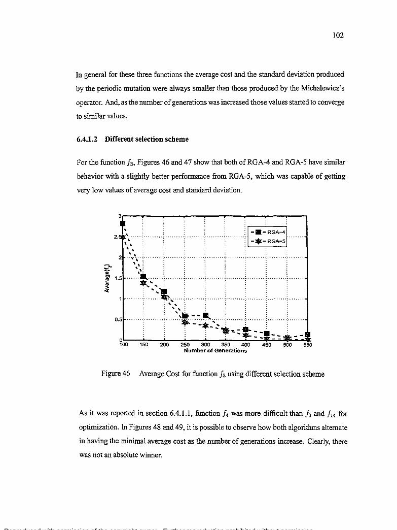
Reproduced with permission of the copyright owner. Further reproduction prohibited without permission.
102
In general for these three functions the average cost and the standard deviation produced
by the periodic mutation were always smaller than those produced by the Michalewicz's
operator. And, as the number of generations was increased those values started to converge
to sirnilar values.
6.4.1.2 Different selection scheme
For the function fs, Figures 46 and 47 show that both ofRGA-4 and RGA-5 have sirnilar
behavior with a slightly better performance from RGA-5, which was capable of getting
very low values of average cost and standard deviation.
' · · · -·-RGA-4 2. l ....... : ......... ; ......... : ......... : .......... : ......... :.
' . . . . . -·-RGA-5
__ 2 \:.x ~p • p l .... l 1 :· :···
t , •••••·t:i<l•••••••l••••••••l•••••••r•••••••:••••••-••••••• 0~ •.•.. ··•·· ..••.•••••• ~~~::}:;;~·~·~·~ _····· .••••..•••.
: : : : .......... •- .... --0~--~--~~--~--~----~--~--~-~~-~-~~ .. ~ 100 150 200 250 300 350 400
Number of Generations 450 500 550
Figure 46 Average Cost for function h using different selection scheme
As it was reported in section 6.4.1.1, function f 4 was more difficult than h and f 14 for
optimization. In Figures 48 and 49, it is possible to observe how both algorithms alternate
in having the minimal average cost as the number of generations increase. Clearly, there
was not an absolute winner.

Reproduced with permission of the copyright owner. Further reproduction prohibited without permission.
1. Jo.
1. : . . :
1.~ .\ ..... ; ... ·····~-· ······-~·-·····--~- ..... ---~---J- B- RGA-4~~----~ ...... .
' ' : : : : : -*- RGA-5 : 1.4 , .. , .. -: ....... -: ....... -: ....... -:- ....... :-... . ... : ...... . ' ' : : : : : : : :
-;.., 1.2 --\\~--------~-------+·······+·······~········~-·······i········l········ .S! '* . . . . . . . 1 ::::: :'-~~~:l ;~ ::t:::: ::: :l:::::::: l::::: ::: l::: ::::: !:: ::::::1::::::: j ::: ............... ·-::.~"~~~· ....... l ................•....... VI , • • *....... ... . ,
:: :.·:::r:::·t:.:.:::r r: ~!"~!:;::~~~:~ - . . . - . - .
0~--~~--~----~--~----~----~--~----~--~ 1 00 150 200 250 300 350 400 450 500 550 Number of Generations
Figure 47 Standard Deviation for function h using different selection scheme
-1900r---~.----~_----7_----~-----~-----~--~~--~----, . . . - .
-192d~-· ..... 1 ........ 1 ... ..... ! . ....... ) ........ ) ...... .. 3 -*!!!!- RGA-4L ...... . , . . . . . ] - -RGA-5j ' : : : : : : . :
-1940 .. , .... ; ........ ; ........ ; ........ ; ........ ; ........ ; ........ ; ........ ; ...... .. ' : : : : : : : :
-1ssè ~~-~~-~-· .. ···~········j· ....... ~-··· .... j- ....... L ....... ) ........ L ...... . .... ~ : : : : : : : -<or
.......... "-·····=···· .. ··=········=········=········=········=····· .. ·=········ a; -1980 0)
~::: :::.:::.:. ·: ~t: "*' ~ ~"! <1 .. :::: .! :. ::::: !·:.:.:: l ::::.: :!! Cl>
~
-2040 ..... ··~ ....... -~- .. ·····~· ....... ~- ...... ·~ ~, ~·j·· .... ~- ... ···j··· .... . :::: :""*-"--~:
-2060 ..... --~ .... ····~········~·······. ~-··· .... ~- ·---~~---~-- r. ··"~·=·~-~~ -2080~--~~--~--~----~--~~--~----~--~--~~
1 00 150 200 250 300 350 400 450 500 550 Number of Generations
Figure 48 Average Cost for function f 4 using different selection scheme
103

Reproduced with permission of the copyright owner. Further reproduction prohibited without permission.
~ c:
..5! = > ID c "E "' "'C c: "' ëi)
12
110
100
90
80
... ~ ~ ~ ~ * ~ :: , ' : - : : ' - : ~- • - RGA-4f -- .. ~--~-.... -~~----T·-------~--;'---r,-----·· 1 ---- -•- RGA-5 .....
~ - ... - ~ -, - - -
--r-:~?J--Is 1 r r . : ~ : ~ \ \~ ....
70
60
. -..... +- ....... ~ ... -... -·i .. -..... \ ........ ·l· .... \ ,; .. ; ~ ~- -~· .. ~-~-~- .... . : : : : : .... _ -· : ~ : : : : : j{ ~ : ~
••••••• ·:· 0 •••••• ·: •••••••• ·:· •• 0 0 •••• :· ••••••• ·:· 0 ••••••• ~- ••••••• ·:- •• , ••••• ~- •••• , ••
~ ~ ~ ~ ~ ~ ; ',~ .. 50
. . - . - . . •-········:·········=·········:·········:·········=·········7·········~·······~·,.·-. . . . . . . . . . . . . . . . . - .
40L---~----~--~--~~--~~--~----~--~~~ 100 150 200 250 300 350 400 450 500 550
Number of Generations
Figure 49 Standard Deviation for function f4 using different selection scheme
104
For the function fi4 , Figures 50 and 51 show that RGA-4 and RGA-5 have similar per
formance indistinctly of the number of generations and the set of probability values. As
it happened with the Rastrigin function, the effect of the probability set is meaningless
specially after 200 generations.
For these three functions there is no clear evidence that one of the two selection schemes
used here has a strong influence in the performance of the periodic mutation operator.
6.4.2 Controller gains optimization
In Garcia et al. (2003, 2006) we used values of Pc = 0.32 and Pm = 0.11 for the business
jet's cases because of convenience rather than they were the best. By using those val
ues the expected number of function evaluations performed by the GA was approximately
1740 and we were able to achieve a running time of 18 minutes for each simulation, sat
isfying in this way a previous limit of 20 minutes that we had set because we were using

Reproduced with permission of the copyright owner. Further reproduction prohibited without permission.
. . : :
-384 ~:······~········~·········l········ ·······-j-···1 =;==~~=:J····~······· ' . .
-385 , ..... ~········~·········~········ ········:·········~·········:·········~······· . . . .
. ....... :. ....... ·=· ........ :. ........ ~ ...... . - - - . . - - . . - . . . . . . . . . .
-386 . ,, .... ; ........ i ......... : ....... . i 1 ' : : : -... '' : : :
~ -387 -~~---~·-······:·······-~········ ........ : ......... : ......... :, ........ ; ...... . . . . . . . . . . . . .
j -388 ::::\1\:::::r:::::::i:::::::: -389 ': ' : :
,; ' : :
- - . . . . . ........ : ......... : ......... :. ........ : ...... . . . - . . . - . . . . . . . . . . . . ........ : ......... :. ........ :. ........ ; ...... . . . . . . . . . . . . . . . . -390 ······•:·····,··=········:···· .... ........ : ......... :. ........ :. ........ : ...... . - . - . * \~ ... il.. : : ~ : ...... T.~ .... -~-~-~,·~-:. : ...... * ...... ~ ..... * ..... ~ ...... -391
. . . -39~0L0----1~5~0----2~0-0----25~0----3~0~0--~3~50~--4-0~0~--4~5~0--~5~00--~5~50
Number of Generations
Figure 50 Average Cost for function f 14 using different selection scheme
14 ~~- .... -~ ........ !········1········~ ........ ~-···j :;: ~:=~l···r··· .. . ' : : : : : : : : ' ..... : ........ : ........ ; ....... ·; ........ : ....... ·: ....... ·: ....... ·: ....... .
. . . . - . . . - . . . - . . . - . - . . ,, : . : : : : . . .2 10 .. , .. ": ....... ·: ....... ·: ....... ·: ....... ·: ....... ·: ....... ·: ....... ·: ...... .
i 8 ·--~~~·······~····"''; ....... ( ...... ; ........ ~ ........ ~ ........ -:- ...... . 'E ' :' : : : : : ... ' : ' . : : : : : . -g 6 ..... ,., .. , .... ·:·""'":'""''';"""":"""":·"""':'"'"'';'""" ... 1: ' : : : : : : : 0
: t\r~?T<.J••• t•···•I•••••••r••• r•••••• ~0~0~--1~5~0--~if--~2~0--~~--~~---i~---!E----!!---~
Number of Generations
Figure 51 Standard Deviation for function f 14 using different selection scheme
105

Reproduced with permission of the copyright owner. Further reproduction prohibited without permission.
106
a PC pentium III, 733Mhz. However, we report here the results obtained by running our
simulations in a PC pentium N, 2.4GHz, with lGbytes of RAM, and using Pc = 0.95
and Pm = 0.20, which were better for our application and provided us with an average
execution tirne of 12 minutes. It is important to highlight that independently of the prob
ability set that we used, periodic mutation was al ways able to outperform the nonuniform
mutation.
CD 0.02 C> e CD > < 0.015
0.01
0.005
....
0,~----72----~3------4~----~5----~6~----~7----~8
Number of Generations
Figure 52 Average costs using a maximum of200 generations
We also used as a benchmark an evolution strategy algorithm (p, + >.) - ES, which is
generally used in floating point optimization. This ES used a recombination operator,
with f-L = 10, >. = 70, maximum number of generations equal 57 and expected rate of
convergence equal one.
Figures 52 and 53 show that the new mutation operator outperformed the other methods
in most of the eight cases. These confirm that the new approach is more effective than
the nonuniform mutation operator by having a mean and standard deviation of the cost
function lower and stable for the who le set of cases, except RGA-4 that in case 8 suffered
a distortion.

Reproduced with permission of the copyright owner. Further reproduction prohibited without permission.
c .2 ;;; > .. c ~ O.Q15
"0 c .!!! U)
0.005
., ........................
l"' l': ,, ......... ( .'. ~- .. '. :" ....... .
1
1
,' \ ' 1
\ '· \ ' 1
,.' \ ....... , .... -:·······,···· 1. .
1 1
1 1 '1
; ' : '
1 . . '\ .. ï :· ....... ~- ........ ,~ .. T .... , ...... . : 1 : 1 1 \ : . :,' : ,; '\
··~;~;··: -~:~~·.·.:.··~/''''''''''1'''' ········4-~:.. ........... ~.
.- . ... : ..... ~·:...-~===-,....--.... 4 5 7 8
Number of Generations
Figure 53 Standard Deviation of the Cost using a maximum of200 generations
107
While using a deterministic parameter control technique on the mutation operator did not
save us from the process of manual tuning, it did improve the effectiveness of our GA in
the aircraft control design problem. In particular, in the combination of our new operator
with the toumament selection scheme, it always generated a small and stable average cost
and standard deviation for the eight cases.
Reproduced with permission of the copyright owner. Further reproduction prohibited without permission.
CHAPTER7
CONSTRAINED STOCHASTIC TOURNAMENT SELECTION SCHEME
Section 4.2 brought to our attention three important ideas that led us to the implementation
of the Constrained Stochastic Toumament Selection scheme discussed in this chapter:
a. methods using a feasibility criterion presented better results than using penalty fac
tor,
b. the effectiveness of a GA was generally increased when the algorithm tried to pro
duce a certain proportion of feasible and unfeasible individuals,
c. to control the proportion of feasible versus unfeasible individuals, sorne articles
reported excellent results when the selection scheme was modified.
Finding a good proportion of feasible and unfeasible individuals is, in fact, a very difficult
task because of the dynamic behavior of GAs . Suppose that we have a population with
N individuals and k unfeasible individuals in the population at generation t. ln addition,
suppose that we are using a toumament selection with a replacement scheme following the
criteria of Deb (2000) for generating the next population t + 1. Then, it is possible, based
on the feasibility characteristic of each element, to have three different types of pair for the
toumament. Each type has different probabilities of occurrence depending on the value
of k (see Figure 54), and each one of them produces different winners due to different
criterion of decision as shown in Table XIII.
Generally, feasible solutions are not known previously when the genetic algorithm starts
to solve the problem; hence, the initial population is frequently populated of unfeasible
individuals. As the population evolves, the reproduction operators find feasible elements
and the proportion of feasible and unfeasible elements changes. While new solutions are
only discovered by the action of crossover and mutation operators, the value of k for the
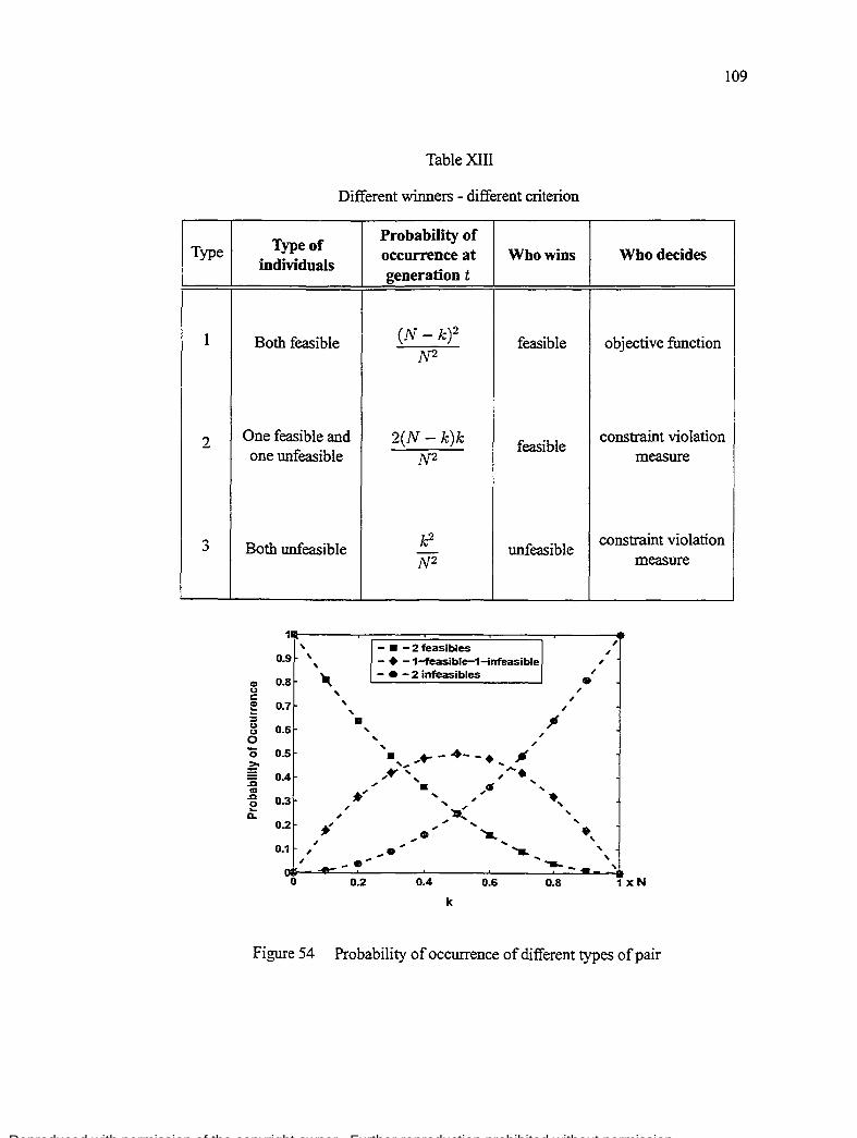
Reproduced with permission of the copyright owner. Further reproduction prohibited without permission.
Type
1
2
3
Table XIII
Different winners - different criterion
Type of individuals
Both feasible
One feasible and one unfeasible
Both unfeasible
1
o. 9
CD 0. 8 u s:::
7
' ' ' ... ' ' '
~ o. :s 8 o. 0
6
o. ô ~ ::ë o. ca .c 0 ~
o.
5
4
3
0.2
o. 1 ,
• '
..... , ,
~ ,
Probability of occurrence at Whowins generation t
(N- k)2 feasible
N2
2(N- k)k feasible N2
k? unfeasible
N2
- • - 2 feasibles - + -1-feasible-1-infeasible - • - 2 infeasibles
, , , ~
' , ,
.... .... -·- -· "' ,, , .... ...... , ...... .... ' . ...., .... . ... , .... .. , ...
~ ' , .... ... ' 'IL. ,• , ... ,. ...... ...
, •
• ' ,
--- e' "'
....... __ 0 0.2 0.4 0.6 0.8
k
Who decides
objective function
constraint violation measure
constraint violation measure
, , ,
' ' ' 1XN
Figure 54 Probability of occurrence of different types of pair
109
Reproduced with permission of the copyright owner. Further reproduction prohibited without permission.
110
next generation can be affected by the selection operator. However, when ali the elements
of the population are unfeasible, as they generally are at the beginning of the process, it
is not possible for the selection scheme to control k. In fact, a selection scheme becomes
important in controlling the parameter k only when the number of unfeasible solutions is
greater than a target value initially set.
A further anal y sis of Figure 54 and Table XIII tells us th at two out of the three types al ways
generate feasible solutions and the same proportion of types are driven by the constraint
violation measure. Suppose now, that we want to find the value of k such as the probability
of unfeasible winner solutions were equal to the probability of feasible winner solutions,
then, by solving Equation 7.1:
we determine that:
k2 (N- kf 2(N- k)k 1\ .. ) = IV .. ) + i\ ·? N- - N-
v'2.N k=--
2
(7.1)
(7.2)
Another way to find the same result is by remembering that ali three probabilities sum 1.
and we can satisfy the condition by determining the value of k when:
(7.3)
Notice that, once k < '1N, the probability of having more feasible solutions as winners
step up and the process may become more involved in exploring specifie feasible regions,
while sorne others may become ignored, especially in cases where we find a great num
ber of disjoints feasible regions or those disjoints sectors are far from each other. Thus,
this kind of method behaves like an over-penalization technique by preserving feasible
individuals and rejecting unfeasible ones.

Reproduced with permission of the copyright owner. Further reproduction prohibited without permission.
111
To soften the effect of over-penalization we can try to achieve a balance between preserv
ing feasible individuals and rejecting unfeasible ones, as mentioned in Gen and Cheng
(1997). So, we can indirectly affect k by applying a balancing approach that is explained
with detail in the next section.
7.1 Constrained Stochastic Tournament Selection
The probability of occurrence of pairs of type 1 and 2, which generate feasible elements
as winners, is higher than the third type when k ::; '(} N. In the case of the toumament of
a feasible-unfeasible pair, the winner is al ways a feasible individual because it is the con
straint violation measure that drives its selection. So, we can try to balance the dominance
of the constraint violation measure by letting, in sorne cases, the objective function decide
who will be the winner, as used in Runarsson and Yao (2000) in the context of the Evolu
tion Strategies algorithms for ranking the population with a bubble-sort-like procedure.
The proposed selection scheme, which we will name Constrained Stochastic Toumament
(CST), consists in choosing the individuals for the next generation by following a stochas
tic toumament criteria of feasibility. This criteria of feasibility is constrained by two fac
tors: k that we already know and ?1 that regulates the balance of the dominance of the
objective function and penalty function, as defined in Runarsson and Yao (2000). Basi
cally. the method can be described by the algorithm of Figure 55.
The CST selection uses a similar strategy as the one used in Deb (2000) when k 2: ~N;
however, once k < ~N then the parameter P1 starts to control the balance of the domi
nance of the objective function and penalty function.
Now, lets define:
v0,N Pk= Prob(k < ---)
2 (7.4)

Reproduced with permission of the copyright owner. Further reproduction prohibited without permission.
Repeat Select randomly two individuals c1 and c2 ;
if both individuals are feasible then
else Select the one with the smaller fitness value:
if kt is less than ~N then Generate a random number r; if r is less than Pt then
else
Select the one with the smaller fitness value; el se
Select the one with the smaller constraint violation; endif
if only one of the individual is feasible then Select it
el se Select the one with the smaller constraint violation;
endif endif
endif until (N individuals have been chosen)
Figure 55 Constraint Stochastic Tournament Algorithm
112
as the probability of k becomes Jess than ~111 at any time or at any generation; Pi} the
probability of occurrence of pair of type i as were defined in Table XIII; P1w the probabil
ity of the individual winning according to the objective function and P6 w the probability
of the individual winning according to the penalty function, as defined in (Runarsson and
Yao, 2000).
Then, the probability that a feasible individual win in a tournament of a feasible-unfeasible
pair, Pwin. is equal to the product of the original probability for type 2 (see Table XIII)
times the probability ofbeing in the region where k;::: ~111 (Equation 7.5).

Reproduced with permission of the copyright owner. Further reproduction prohibited without permission.
rr::.TV "fk v .c,_ 1 "> --. - 2 '
113
(7.5)
Or, equal to two terms. Both terms have a common factor th at consists in the product of the
original probability for type 2, times the probability of being in the region where k < v;N. The first term is also affected by the probability of the individual winning according to the
objective function times the probability of comparing the pair using the objective function.
The second term is multiplied by the probability of the individual winning according to the
penalty function times the probability of comparing the pair using the constraint violation
measure (Equation 7 .6):
After sorne simplifications and considering that for a feasible individual Pç)'u: = 1, Equa
tion 7.6 becomes:
(7.7)
Since we are only interested in reducing slightly the number of feasible individuals as
winners when k < '1N just to avoid a drastic drop-off of unfeasible elements in the next
generation, then we have to control the third term in Equation 7.7. While it is not possible
to manipulate P1w, we can doit with P1. When we have extreme values of P1w = 0 and
P1w = 1, Equation 7.7 reduces to Equations 7.8 and 7.9 respectively:
(7.8)
and,
(7.9)

Reproduced with permission of the copyright owner. Further reproduction prohibited without permission.
114
Thus, both Equations 7.7 and 7.8 show that when the probability of a feasible individual
winning according to the objective function is low, then ?1 controls the drop-off of fea
sible winners, and, therefore, its value should be low enough to do the job correctly in
our algorithm. Thus, ?1 acts as a constraint of the reduction of feasible elements in our
selection scheme.
7.2 Experimental Study
To validate our approach, we have conducted two kinds of experimental studies. In the first
one, we compare the search performance of our method on commonly used benchmark
functions as those presented in Appendix 2 against the results reported in other articles.
The second test uses a constrained model of Bombardier for optimization. As it was
explained in the first chapter, the interest of our research is not GA in the long run or its
asymptotic behavior, but GA in the short run and with real engineering problems. Due to
the impossibility of having results from other researchers using our simulation model, we
decided to apply to our problem the evolution strategy algorithm proposed by Runarsson
and Yao (2000), which was available on Internet, and compare its results with the one
produced by our GA
7.2.1 Benchmark Functions
The objective of this study is to show how GA perform in the long term comparing to
other algorithms proposed by other researchers. Although the articles did not use the same
parameter values and conditions for testing, we decided to do it for our experiment. By
same conditions, we mean, for example, to set up the same number of generations and the
same population size for the whole set of functions, which can be viewed as performing
the same number of evaluation functions.
The parameter values of the GA used for this test were set up to 40 individuals for the

Reproduced with permission of the copyright owner. Further reproduction prohibited without permission.
115
population size, a Pc = 0.90, a Pm = 0.05, ab factor equal to 5 for the nonuniform mutation
as it was suggested in (Michalewicz, 1996), an elitism criteria, a maximum number of
5000 generations and a number of 50 trials in order to get sorne useful statistics. We
named this implementation using our new technique Constraint Stochastic Toumament
Genetic Algorithm (CST-GA),
To set a convenient value for P1, we started trying a value equal to Pm· and then we used
other values. Finally, the first one was the one that generated the best results.
Table XIV presents the results for eleven test functions reported in the seven articles ana
lyzed in chapter five and the optimal values. Only Kocis and Whiten (1997) and Hamida
and Schoenauer (2000) reported the results for the who le set of eleven functions.
Table XIV
Results reported in seven articles for eleven test functions
1 Func. 1 Al A2 A3 AS A6 A7 Optimal
1 -15 -14.7864 -15 -15 -15 -15 - -15
2+ 0.79953 0.800781 0.80248 0.787933 0.803619
s+ - 0.9997 1 1
4 -30664.5 - -30665.6 -30665.5 -30665.537 -30659.997 -30665.539
5 - - 4707.52 - 5126.498
6 -6952.1 - -6961.81 -6961.81 - -6961.814
7 24.69 24.62 24.31 24.36 24.338 24.37248 - 24.306
s+ 0.095825 - 0.095825 0.095825 - 0.095825
9 680.642 680.91 680.65 680.63 680.63 680.634 680.63
10 7377.976 7147.9 7083.21 7095.15 7066.36 7060.221 7049.331
11 0.75 0.75 0.749001 0.75
As can be seen from Table XV, our algorithm, using the constrained stochastic toumament
selection method, performed very weil for most test functions as compared with the best
results produced by the seven articles. Thus, the new method is capable of retuming an
optimal very close to the true optimal, except for function number 10 which was also

Reproduced with permission of the copyright owner. Further reproduction prohibited without permission.
116
di ffi cult for the other methods as we can observe in Table XIV.
Table XV
Comparative results of the new method
1 Function 1 Optimal CST-GA A1-A7
1 -15 -15.00000 -15
2+ 0.8033553 0.80359 0.80248
3+ 1 1 1
4 -30665.5 -30665.53217 -30665.6
5 5126.4981 5126.61403 4707.52
6 -6961.81 -6961.80966 -6961.81
7 24.306 24.35632 24.31
s+ 0.095825 0.09583 0.095825
9 680.63 680.63253 680.63
10 7049.331 7064.00621 7060.221
11 0.75 0.74992 0.75
7.2.2 Practical Flight Control Design Problem
Another way to madel a practical flight control design problem is by using standard per
formance measures that are usually defined in terms of the step response of the system
as part of the fitness function and the handling qualities criteria as part of the constraint
functions.
The fitness function we have considered are the peak time Tp, that partially measures
the swiftness of the response; the percent overshoot PO, and the settling time Ts that
measures the similarity with which the actual response matches the step input. Finally, we
have added a fourth criteria which measures the case of underdamped systems for which
the second peak should not overpass certain band, which we denote as Ymin·

Reproduced with permission of the copyright owner. Further reproduction prohibited without permission.
117
fitness = fpo + frP + frs + fYmin (7.10)
To consider the same influence of each feature in the value of the fitness we have used
sigmoid functions to norma1ize their values, as is shown below and in Figures 56, 57, 58,
and 59:
(7 .11)
(7.12)
(7.13)
( ( ( a;Ymjn ))) -1 fymin = 1 + e - maxym:n X3 (7.14)
where
maxPO = 0.40; maxTp = 2.-5;
maxTs = 3.5; maxYmin = 0.03
To show the benefits of using our new selection method we implemented two GAs with
the same Blend-Xover operator and Pc = 0.95, the same periodic mutation operator and
Pm = 0.05, but with a different selection strategy. CST-GA used our approach and SFC
GA used the feasibility criteria implemented in (Deb, 2000).
We also used a third algorithm, named Stochastic Ranking Evolution Strategy (SR-ES),
that was reported in (Runarsson and Yao, 2000), and has produced excellent results in
the optimization of the mathematical functions. For this algorithm, instead of the original
values, we used 11 = 10, À = 70 and a maximum number of 50 generations, because we
were limited for a maximum of 4000 evaluation functions that our GAs used.

Reproduced with permission of the copyright owner. Further reproduction prohibited without permission.
0.9
0.8
0.7
0.6
-~ 0.5
0.4
0.3
0.2
0.1
PO
Figure 56 Sigmoid function for the oversboot of a step function response
0.9
0.8
0.7
0.6
J: 0.5
0.4
0.3
0.2
0.1
0 0 0.5 1.5
T p
2.5 3
Figure 57 Sigmoid function for the peak time of a step function response
118

Reproduced with permission of the copyright owner. Further reproduction prohibited without permission.
119
1
0.9
0.8
0.7
0.6
.? 0.5
0.4
0.3
0.2
0.1
0 1.5 1 2 2.5 3 3.5 4
T s
Figure 58 Sigmoid function for the settling rime of a step function response
0.9
0.8
0.7
0.6
0.4
0.3
0.2
0.1
0~----_.------~~~--~------~----~ -0.15 -0.1 -0.05 0 0.05 0.1
Y min
Figure 59 Sigmoid function for the second peak of a step function response

Reproduced with permission of the copyright owner. Further reproduction prohibited without permission.
120
The comparison of our approach with the SFC-GA shows the impact on the reduction of
the standard deviation of the optimal values produced. The comparison with the SR-ES
allows us to see an application of the balancing strategy in GA different from the one used
in the SR-ES. We collected the results of 50 iterations of each one of seven cases: 24, 44,
64, 84,104, 124 and 144. Each iteration took 14 minutes torun in a PC pentium IV of
2.4GHz and lGbytes ofRAM.
Cl earl y our GA did find the smallest cost in two ofthe seven cases, and it was not so distant
in the other cases as it was SFC-GA in case 84 (see Figure 60). However, the behavior
of its standard deviation and average cost were better and more stable than the two other
algorithms (see Figures 61 and 62).
0.169
0.168
0.167
0.166
- 0.165 "' 0 u
0.164 -;; CD
IJl 0.163
0.162
0.161
0.16
....... ES-SR ..... SFC-GA
• -+- · CST-GA
Casenumber
Figure 60 Best Cost using CST-GA
The step response for each one of the seven cases, shown in Figures 63, 64, and 65,
presents the convenience and usefulness of the new model for the Bombardier's problem.
Besides the fact that the handling qualities criteria have been satisfied, this model con
tributes to the designer with a flexible way of controlling the characteristics of the step
response of the system.

Reproduced with permission of the copyright owner. Further reproduction prohibited without permission.
c: .2 fti > CD
Q
"E .. "CS c: .. U)
1.4rr----~------~----~----~----~-----r0
1.2
0.8
~ ......... 0.6 - --
0.4
0.2
-24
...... ES-SR
@· SFC-GA -·-CST-GA ••
)~ ·- ,---' --__ _,- ~,,,; ~.. -
_/+- ~-:.>:-.::-~ -.. -\ -'* ~ --~ ,_ ' ':_
~ 1 ' : ~-,' '--
~-, '': _-, ,._ ~ ,: ~ ~
i_
84 104 124
Case number
Figure 61 Standard Deviation using CST-GA
0.9rr----~------~----~----~----~-----r~
0.8
0.7
" .... ES-SR · · 0· · SFC-GA -·-CST-GA
•
~ 0.6 • c; _ _.'!1-.. '-~ 0.5
~ 0.4 --------- .... ~--~.>- <-,,.··'''··-. __ •········•. _: '•····' ::& -- -· ---
0 • '., .. - l,' ' "', .3 -- -.____ - 1-- '-
0.2 ----- --. __ --~' ,' ,-~~-.. -- --·-·-·.:.·· . 0.1L..J... ____ __._ ____ __._ ____ __,_ ____ ___. __ __,_ __ __,___J
24 44 64 84 104 124 144 CaseNumber
Figure 62 Average Cost using CST-GA
121

Reproduced with permission of the copyright owner. Further reproduction prohibited without permission.
--------'S::..;t=ep Resp~o:.:cn.:.;:s:..::e _______ _ 1.4'
1.2 r:==24l ~
o~-------~----~----~----0 2 4 6 8
Time (sec)
Figure 63 Step Response for cases 24 y 44
1.4 ,-~---·----
1.2 ~
CD
~ 0.8
a. ~ 0.6
1
0.4.
! 1
o.< J :1
o!.l 0 2 4 6 8
Time (sec)
Figure 64 Step Response for cases 64 y 84
10
10
122

Reproduced with permission of the copyright owner. Further reproduction prohibited without permission.
1.2
CD
~ 0.8
-a : E o 6~ < - i
0.2 ~
a~' ------------~--------------------0 2 4 6 8
Time (sec) 10
Figure 65 Step Response for cases 104, 124 y 144
123
When we compare the step response results obtained by using the original model of Bom
bardier versus those given by our proposed model, it is possible to see more clearly the
convenience of the constrained model. In five out of seven cases, the step response of
our model had a smaller overshoot, and a smaller settling time (see continue line from
Figure 66 to Figure 72) in six out of seven.

Reproduced with permission of the copyright owner. Further reproduction prohibited without permission.
Step Response 1.4~---~--- ---·-- ----- --~--~
1.2·
1-
~ 0.8 ~
~ a. ~ O.G-
0.4•
0.2'
0 0
Figure 66
.. ··----~·- -------~-- -·- ·- - -----~----··--___.._ ___ -- ~-
2 3 4 5 6 7 8 10 Tlme (sec)
Case 24 using unconstrained and constrained model
Step Response 1.4r---..---.-----,.----.---.-----.---....----.---.--""ï
... 1.2 1 \
~ 0.8
~ a. E ' < 0.6 1
0.4
0.2
' ' ---- --- ----
0o~L---~----2L---~-----4L---~s----~G----~7----~a~---L--~1o
Tlme (sec)
Figure 67 Case 44 using unconstrained and constrained model
124

Reproduced with permission of the copyright owner. Further reproduction prohibited without permission.
Step Response 1.4 '-·---~----,---- ---~--------------:---·-r~---- --------
1.2
1 -
., 0 8 ·-~-ëi. E < 0.6-
0.4"
0.2-
~- constnolned 1 - - unconstralned
---
0 -------'-- -----"-- --- __ , -------------·---- -~-----"----------- --------0 1 2 3 .,. 5 6 7 8 9 10
Time(sec)
Figure 68 Case 64 using unconstrained and constrained model
Step Response 1.4-------------------------------------------------------
~ 0.8~ :ê ' ëi. E ' < 0.6:-
3
j constrained 1 - - unconstrained
4 5 6 7 Time (sec)
s 9 10
Figure 69 Case 84 using unconstrained and constrained model
125

Reproduced with permission of the copyright owner. Further reproduction prohibited without permission.
Step Response 1.4 ----~ --------~~·:-------,~~----r----~--~----- · ---~-- ---- ·-··---- ---
1.2'
~ o.s: :ê c. E < 0.6 1•
0.4:·
0.2.
0 ' ------------ ·----~-- ·--0 1 2
----
1 constralned 1 -:- - unconstralned
4 5 6 7 Time(sec)
8 10
Figure 70 Case 104 using unconstrained and constrained model
Step Response 1.4,~--------------------------------------------------------
i
~ o.si· :ê c. E t
< 0.6•·
0.4 ~
0 0
,.. 1 '
1
Figure 71
~- constrained 1 - - unconstrained
2 3 4 5 6 7 8 10 Time(sec)
Case 124 using unconstrained and constrained model
126

Reproduced with permission of the copyright owner. Further reproduction prohibited without permission.
Step Response 1.4~--~~--~--------------~----~---------------r-----
1.2
~ 0.8~ ~ 1
"ë. E : < 0.6:·
0 0
, ' '
3 4 5 6 ï 8 10 Time (sec)
Figure 72 Case 144 using unconstrained and constrained model
127

Reproduced with permission of the copyright owner. Further reproduction prohibited without permission.
CHAPTER8
BAYESIAN ADAPTIVE GENETIC ALGORITHM
The efficiency and effectiveness of Genetic Algorithms are highly determined by the de
gree of exploitation and exploration kept throughout the run. In Section 4.3, we presented
a general classification of methods for changing the value of parameters of GAs. On the
path of adaptive parameter settings of this taxonomy (Figure 28), severa! techniques have
been proposed to control the exploitation/exploration relationship (EER) in order to avoid
the premature convergence.
Despite the availability of a significant body of expertise and knowledge as a result of
severa! years of empirical studies, and to the best of the authors knowledge, there is no
any study in the literature that reports the use of Bayesian Network (BNs) for adapting
GA parameters in order to induce a suitable EER. So, in the present chapter, we present
a model for controlling the adaptation of parameters setting of a Real-Valued GA based
on a Bayesian Network approach. We first introduce however the mode! of an adaptive
GA based on Bayesian Network. This is followed by an overview of the different diversity
measures that have been proposed for the GA community. Then, the definition of the mod
ified Simpson's Diversity Index and our approach in order to apply the index to numerical
optimization problems using RGAs are described. A new method for termination of the
optimization process based on the modified Simpson 's index is completely detailed, and
the results of its successful application are also explained. Finally, the description for the
implementation of a new adaptive nonuniform mutation operator and its inclusion in a GA
named Probabilistic Adaptive Genetic Algorithm (PAGA) are explained.
8.1 Adaptive GAs based on Bayesian Network
Over a number of years, a great body of human expertise and knowledge on GAs has been
developed as a result of many empirical studies. Though most of this information is gen-

Reproduced with permission of the copyright owner. Further reproduction prohibited without permission.
129
erally uncertain, vague, incomplete, or ill-structured, it is possible to use sorne techniques
capable of working with this type of knowledge like, for example, fuzzy logic controllers
(Am one et al., 1994; Herrera et al., 1994; Lee, 1990; Xu et al., 1994; Herrera and Lozano,
1996).
Whi1e fuzzy logic controllers deal with uncertainty contained in the vague descriptions of
the experts knowledge, Bayesian Networks (BNs) deal with the association of real num
bers with the uncertainty in the members of a set of mutually exclusive and exhaustive
alternatives (Neapolitan, 1990). Although techniques like fuzzy logic controllers use nu
merical representations of uncertainty, they disregard probability calcul us, computing the
uncertainty of any formula as a function of the uncertainties of its sub-formulas (Pearl,
1988); moreover, their rules can be interpreted as summaries of past decisions. In the case
of Bayesian Networks, rules are interpreted as conditional probabilities expressions and
they represent summaries of factual or empirical information. Besides, as Pearl ( 1988)
asserts, intensional systems, like BNs, have no problem handling bi-directed inferences
and correlated evidence.
Although BNs seems more suitable to handle the knowledge obtained from the stochastic
behavior of GAs, difficulty in setting up conditional probabilities and the high demand on
computation have been probably the reasons wh y BNs have not been applied for adapting
GA parameters.
8.1.1 Description of the Bayesian Network
Bayesian or Belief Networks are directed acyclic graphs (DAG) of nodes, each represent
ing a random variable with a fini te domain. The directed arcs signify the existence of direct
causal influences between the nodes, and the strengths of these influences are quantified
by conditional probabilities (Pearl, 1988) (see Figure 73).
One of the advantages of using BNs is that an arc from one node A to a node B can express

Reproduced with permission of the copyright owner. Further reproduction prohibited without permission.
P(A)
P(CIA)
P(DIB,C)
Figure 73 Bayesian Network examp1e
the idea of "A causes B" (Figure 73). Moreover, according to Pearl (1995):
"the human intemally structures his or her causal knowledge in his or her own persona! Bayesian network, and that he or she perforrns inference using that knowledge in the same way as Pearl's message-passing algorithm (Pearl, 1988)."
130
Hence, by using causal relationships we can try to formai ize and model our partial reason
ing and knowledge about RGA behavior in a Bayesian network.
Another advantage of BNs is that using causal relationships may allow us to maximize
the representation of conditional independence and construct a more compact and simple
model (Korb and Nicholson, 2004 ). For example, the joint probability over the random
variables of Figure 73 can be computed via the chain rule as:
P(A, B, C, D) = P(A)P(BIA)P(CIB, A)P(DjC, B, A) (8.1)
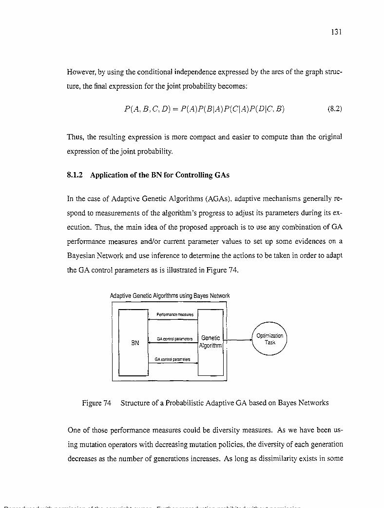
Reproduced with permission of the copyright owner. Further reproduction prohibited without permission.
131
However, by using the conditional independence expressed by the arcs of the graph struc
ture, the final expression for the joint probability becomes:
P(A, B, C, D) = P(A)P(B\A)P(CIA)P(D\C, B) (8.2)
Thus, the resulting expression is more compact and easier to compute than the original
expression of the joint probability.
8.1.2 Application of the BN for Controlling GAs
In the case of Adaptive Genetic Algorithms (AGAs). adaptive mechanisms generally re
spond to measurements of the algorithm's progress to adjust its parameters during its ex
ecution. Thus, the main idea of the proposed approach is to use any combination of GA
performance measures and/or current parameter values to set up sorne evidences on a
Bayesian Network and use inference to determine the actions to be taken in order to adapt
the GA control parameters as is illustrated in Figure 74.
Adaptive Genetic Algorithms using Bayes Network
Pertormance measures
GA control parameters Genetic Optimization BN Task Algorithm
GA control parameter;
Figure 74 Structure of a Probabilistic Adaptive GA based on Bayes Networks
One of those performance measures could be diversity measures. As we have been us
ing mutation operators with decreasing mutation policies, the diversity of each generation
decreases as the number of generations increases. As long as dissimilarity exists in sorne

Reproduced with permission of the copyright owner. Further reproduction prohibited without permission.
l "'? .)_
level, crossover operators can be capable of doing the exploitation and a little exploration
of the search space, provided that convergence has not been reached. So, having a met
rie of dissimilarity becomes very important in order to evaluate the effectiveness of the
crossover operator as the number of mutations at each iteration decreases, and to detect
the convergence of the algorithm. Moreover, the GA can decide to stop its optimization
process if it is not longer useful because of lack of diversity and saving cpu ti me. It is also
important to consider that as mutation rate decreases, if the dissimilarity among the genes
decreases then to bring forth population diversity for further exploration of the search
space becomes harder and harder. Thus, the following section presents a small overview
of different diversity measures that have been presented for different researchers.
8.2 Diversity Measures
The explotationlexploration relationship of GAs is strongly related with the diversity of
every generation. GA community reports several diversity measures (Bedau et al., 1995;
Herrera and Lozano, 1996) that describe the state of the population, and can be classified
in two types: genot;.pic diversity measures (GDMs) and phenotypic diversity measures
(PDMs). Whilst GDMs try to describe the variation or lack of similarity between the ge
netic material held in the population, e.g., alleles, chromosomes, etc, PD Ms are concerned
about the fitness of the chromosomes (Herrera and Lozano, 1996).
8.2.1 Genotypic Diversity Measures
Among the different approaches for GDMs found in the literature, those based on Eu
clidean Distance, and Dispersion Statistical Measures have been applied to Real-Coded
GA.
Herrera and Lozano (1996) propose one measure based on the Euclidean distances of the
chromosomes in the population from the best one and is denoted as ED:

Reproduced with permission of the copyright owner. Further reproduction prohibited without permission.
where
ED = d- dmin dmax- dmin
and P is the population composed by real-coded chromosomes.
(8.3)
The interval of the values of ED is [0, 1] and when ED is low, most chromosomes in the
population are concentrated around the best chromosome and therefore convergence is
achieved. On the contrary, if ED is high most chromosomes are not biased toward the
current best element.
In Herrera et al. (1994), the authors present a diversity measures for real coding based on
dispersion statistical rneasures. They are based on the variance average of the chromo-
sames:
(8.4)
and the average variances alleles:
'"'N '"'L ( -)') 41, 4. = L....-j=l L....-i=l sij - sj -
" ~. L · N (8.5)
where
(8.6)
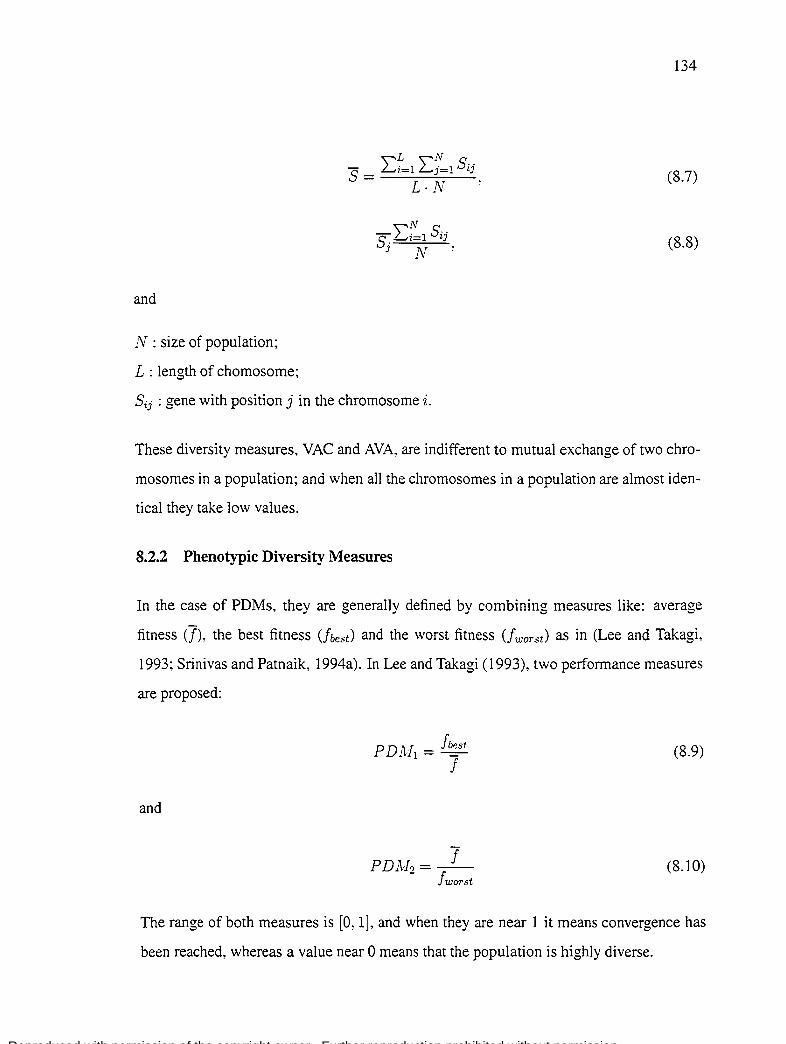
Reproduced with permission of the copyright owner. Further reproduction prohibited without permission.
134
(8.7)
(8.8)
and
N : size of population;
L : length of chomosome;
sij : gene with position j in the chromosome i.
These diversity measures, VAC and AVA, are indifferent to mutual exchange of two chro
mosomes in a population; and when ali the chromosomes in a population are almost iden
tical they take low values.
8.2.2 Phenotypic Diversity Measures
In the case of PDMs, they are generally defined by combining measures like: average
fitness (Ï), the best fitness Ubesd and the worst fitness (J worst) as in (Lee and Takagi,
1993; Srinivas and Patnaik, 1994a). In Lee and Takagi ( 1993), two performance measures
are proposed:
(8.9)
and
1 PDAJ.) = --- fworst
(8.1 0)
The range of both measures is [0, 1], and when they are near 1 it means convergence has
been reached, whereas a value near 0 means that the population is highly diverse.

Reproduced with permission of the copyright owner. Further reproduction prohibited without permission.
135
\Ve can summarize sorne characteristics of the diversity measures presented in this section
as:
1. l'AC and A VA use the middle point of the population as a reference point for their
computation, and they use an average operation to get that middle point.
2. PD l'vh and PD l\12, use the mean of the objective function as a reference point of
their computation,
3. E D uses the genes of the best chromosome as a point of reference and the Euclidean
distance for its computation.
AU these indexes were tested with different problems and the results were totally different
or useless for getting sorne clue in order to use them in a Bayes Network. Several factors
like the function to be optimized; the number of generations that we let the algorithm to
run; the type of mutation operator and severa! values of Pc and Pm were studied during the
simulations. Figures 75 to 83 are sorne of the results that illustrate our remarks.
ED did not give any clue about convergence or diversity (see Figures 75 to 79). In sorne
cases, PD J\!1 and PD Ah gave sorne information about convergence (Figures 80 and 81)
but not about diversity. And, in other cases, they provided a low peak showing the lack
of diversity and the arrivai of convergence as in Figures 82 and 83. VAC and AVA were
completely useless when we applied them to our GAs and we decided not to show them
he re.
After all these results, we made up our mind to propose the application of an index from
ecolo gy called Simpson 's Diversity Index. But for its application to optimization problems
it was necessary to implement an innovated procedure. The following section deals with
this new index that was presented in (Garcfa et al., 2005).

Reproduced with permission of the copyright owner. Further reproduction prohibited without permission.
0.9
0.3
0.2
0.1
ED ---pmenvelope
oL-----~------~----~~------~----~ 0 500 1000 1500 2000 2500
Generation Number
Figure 75 ED behavior using h and non-uniform mutation
!! ë 0.5 :::;,
0.4
0.3
0.2
0.1
0 0 500 1000 1500 2000 2500
Generation Number
Figure 76 ED behavior using ! 1 and periodic mutation
136

Reproduced with permission of the copyright owner. Further reproduction prohibited without permission.
1r---~----~--~======~--~ 1-· :~ __ J 0.9
0.8
0.7 -·.· .. -.~ :...:... · ..... ,.
0.2
0.1
0~------~------~------~------~------~ 0 500 1000 1500 2000 2500
Generation Number
Figure 77 ED behavior using h and non-uniform mutation
1~~-----r------~------~~------~------~
0.9
0.8
0.7
0.3
0.2
0.1
0o~------50~o-------1-o~o-o~--~1~5~oo-------2-o~o-o------2~5oo
Generation Number
Figure 78 ED behavior using h and periodic mutation
137

Reproduced with permission of the copyright owner. Further reproduction prohibited without permission.
0.9 1-· =~--1 0.8
0.3
0.2 =·
0.1
OL-----~----~----~--~~----~----~ 0 1 00 200 300 400 500 600
Figure 79
0.9
0.8
0.7 t
0.6 rn 1. •• ••
'Ë 0.5 ~- .. :;:) .:
"- . 0.4 1. :''
r· ... : 0.3 1
1 •• '·:. :· 0.2 ~-: .-:·. ~ .. ~ 0.1 \
Figure 80
Generation Number
ED behavior using h and 500 generations
PDM1
--pmenvelope
-- -fobj
.· .. -·
.-
200 300 Generation Number
PD M1 behavior using h and 400 generations
138

Reproduced with permission of the copyright owner. Further reproduction prohibited without permission.
0.9
0.8
0.7 . . ·
0.6 .•.
~ 0.5 ~ ··:·:. =.~·- . 0.4 :· .\ ~-~· 0 .. 3 ........ ..
0.2 1
' 0.1 ' '
·.:···J·, :· .... ~ ',·.a(:
100 200 300 Generation Number
PDM2
--pmenwiopo
- - -fobj
400 500
Figure 81 PD lv12 behavior using fa and 400 generations
0.9
0.8
Figure 82
100
... -,_ ... -.~ PDM1
: . ,. --pmenwiopo .. : ;_· .. · •.
.. ·.: .. ·:: . : ·. :'~:~·.\.-- -fobj .. :-.........
·~ :.::-.: .. :.., .. . ..
200 300 400 500 600 Generation Number
PD M1 behavior using f 5 and 500 generations
139

Reproduced with permission of the copyright owner. Further reproduction prohibited without permission.
140
0.9 ._.:]:~:;_ • _: •• ".o;
- .....
' . . 0.1 • •...
oL-~~~~~~~~w.--~~----~----~
0 100 200 300 400 500 600 Generation Number
Figure 83 PD M2 behavior using fs and 500 generations
8.3 Modified Simpson's Diversity Index (mD)
This new index is inspired by Simpson's Diversity Index, which is a measure of diversity,
and it is often used to quantify the bio-diversity of a habitat in ecology. lt takes into
account the number of species present, as well as the abundance of each species.
There are different ways to quantify biological diversity; one of th ose is to consider two
factors like richness and evenness. While, richness measures the number of different kinds
of organisms present in a particular area (e.g. the number of different species present),
evenness compares the similarity of the population size of each of the species present.
Richness counts the number of species per sample, and the more species are present in a
sample, the ri cher the sample is. lts measure does not depend on the number of individuals
of each species. lt assigns as much weight to those species with very few individuals as
those with many.

Reproduced with permission of the copyright owner. Further reproduction prohibited without permission.
141
Even ness gives an idea of the relative abundance of the different species that makes up the
richness of an area. For a better understanding of these two terms, suppose we have two
different sampled fields of wildflowers. In Table XVI, we can see the distribution of the
individuals for each species and for each sample.
Table XVI
Sampled fields of wildflowers
Number of individuals
Flower Species Samplel Sample2
Daisy 300 20
Dandelion 335 49
Buttercup 365 931
Total 1000 1000
Both samples have 3 species, so they have the same rich ness. Although both samples have
the same total number of individuals (1 000), the first sample has more evenness than the
second because the total number of individuals in the sample is quite evenly distributed
between the three species. In the second sample, there are few daisies and dandelions
present and most of the individuals are buttercups. Therefore, we can consider sample 1
more diverse than sample2.
Simpson's Diversity Index (D) is a measure of diversity which takes into account both
richness and evenness. Generally there are three closely related definitions for D. One
way is that D measures the probability that two individuals randomly selected from a
sample, with replacement, will belong to the same species (or sorne category other than
species).
(8.11)

Reproduced with permission of the copyright owner. Further reproduction prohibited without permission.
where
ni = the total number of organisms of a particular species i;
S the set of different species; and
N = the total number of organisms of ali species
142
With this index, 0 represents infinite diversity and 1, no diversity. That is, the bigger the
value of D, the lower the diversity. For our purpose, it is rouch better to subtract from 1, so
the greater the value, the greater the sample diversity. and it is still in the range of 0 and 1:
mD= 1- D (8.12)
8.3.1 How to apply mD
To apply the modified Simpson 's Diversity Index (mD), we need to have sorne categories
or classes. The question is, how to do a categorization among chromosomes of each
generation that could be useful to compute mD. The following anal y sis will help us to
figure it out.
Until now, we have used Real-Coded GAs with non-uniform or periodic mutation oper
ators in combination of a blend crossover operator and a toumament selection method.
Both mutation operators have a mechanism for decreasing the mutation interval, and both
have also a very interesting behavior. First, as the interval gets smaller than the one used
in previous generation, the GA is still able to find new optimal individuals but this action
stops several generations before to reach [\'. And, second. in the case of periodic muta
tion, when the mutation interval is increased shortly along the final stage of the searching,
sometimes for small values of jumps the GA still produced optimal individuals and sorne
times not. Thus, we can say intuitively that the GA is converging sorne generations before
reaching N, and for small values of mutation at the final stage there is sorne degree of
dissimilarity among the genes of chromosomes that allows the crossover operator to mate
individuals and to further the exploitation of the search space and yield a better best-so-far

Reproduced with permission of the copyright owner. Further reproduction prohibited without permission.
143
performance (Huang, 2002). In other words, we can expect that even when chromosomes
are very close to each other, specially to the best one, finding a new optimal is feasible as
long as sorne degree of dissimilarity among their genes exist.
We may interpret these observations and propose two hypotheses as follows:
Hypothesis A There exists a group of classes of chromosomes around the best individual
with sorne characteristics that their diversity becomes cri ti cal for the convergence of
a RGA using a decreasing policy of mutation step;
Hypothesis B When the diversity ofthis group of classes of chromosomes becomes lower
than sorne value KmD then the likelihood that convergence happens is maximum.
To proof these two hypotheses, we propose to measure the diversity of the classes of
chromosomes that are formed in a very small sector around the current best optimal indi
vidual. To produce speciation or categorization we propose, first, to divide this region in
five classes depending on the absolute value of the distance between every gene of each
chromosome and its respective gene of the best fit individual in the population:
(8.13)
where dij is the distance between gene j of chromosome 'Ï, sij' and gene j of the best
chromosome, Sbestj.
We set up a limit of distance for each class. Let us say the limits are those presented
in Table XVII. Then, we count the number of locations at which corresponding genes
are inside each interval, and, let us say also, that we are only interested in having classes
where the number of similar genes is greater or equal to 60%. Renee, each class will be
composed by those chromosomes with 60% or more genes that are similar and they are
inside the intervals defined in Table XVII.

Reproduced with permission of the copyright owner. Further reproduction prohibited without permission.
144
Table XVII
Classes intervals
1 Class 1 Interval
dij ~ é
2 é < dij ~ 5é
3 5é < dij ~ 1 Oé
4 10E < dii ~ 50E
5 50€ < dij ~ 100€
8.3.2 Experiments
We tested our implementation to get the modified Simpson's Diversity Index with two
configurations of GAs: one with non-uniform mutation and the other with a periodic mu
tation. Both GAs have in common a blend crossover operator, a tournament selection
scheme and a population size of 40 individuals. We used a value of E" = 0.00001 similar
to the accuracy that we want for our results.
Every time that we used mD with a GA using non-uniform mutation, we were able to
geta value of 0 (KmD) when the GA reached the convergence. More interesting was the
fact that for each function optimization when the difference between two or more optimal
individuals started to be less than 0.00001, mD was always zero, which by coïncidence
was the li mit of the first class. It seems that the li mit of this class may allow to tune the
precision of the optimization (see Figures 84, 85 and 86). So, we supported hypothesis A
and hypothesis B empirically by using non-uniform mutation.
Using periodic mutation was different but still very useful. As we can observe in Fig
ures 87 to 90, when mD started to get values approximately lower than 0.20 (KmD) then
the convergence of the optimization started to be reached. So. hypotheses A and B are
also supported with these tests for periodic mutation.

Reproduced with permission of the copyright owner. Further reproduction prohibited without permission.
.!! ë :::1
mD --pmenvelope
-- -f1
1000 1500 2000 2500 Generation Number
Figure 84 mD behavior, JI, Pc = 0095 and Pm = 0005
1
Oo9
Oo8
Oo7
Oo6 1
Oo5 ~ 1
Oo4 1
0.3 1
0.2 1
1
Oo1 • 0
0
• 100
mD
-- pdenvelope
-- -fs
· .. · .. Oo
0 0
o"o
200 300 400 500 600 Generation Number
Figure 85 mD behavior, fs, Pc = 0095 and Pm = 0005
145

Reproduced with permission of the copyright owner. Further reproduction prohibited without permission.
0.9
0.8
0.7 1
0.6
"'
--: . ........ .
'
mD --Pmenvelope
-- -f14
~ 0.5 1
::::1
.!!! ë ::::1
l
0.4 -0.3
0.2
0.1
0 0
' ' ' -. 50 100 150
Generation Number 200
Figure 86 mD behavior, !14, Pc = 0.62 and Pm = 0.11
0.9 1
0.8 1
0.7
0.6
0.5 -0.4 1 . 0.3 1
' 0.2 ' ' mD
' 0.1 --. 0
0 100 200 300 400 500 600 Generation Number
Figure 87 mD behavior, !1, Pc = 0.95 and Pm = 0.05
146

Reproduced with permission of the copyright owner. Further reproduction prohibited without permission.
.!!! ë :::.
.!!! ë :::.
1 .. 0.9 -
' 0.8 1 •
J 1 - ..
0.7 1.
0.6 {
.. 0.5
1
1
0.4
0.3 1 -0.2
0.1 ' ' 0 ' 0
Figure 88
0.9
0.6 1
0.5:
1 0.41
1 0.3
1 0.2
' 0.1 .. 1
' 0 0
·. mD · .. -'::··: . --pmenveJope
·- -- -f.c
.. , .-. . . -: : -
..
50 100 150 200 250 Generation Number
mD behavior, / 4 , Pc= 0.32 and pm= 0.11
100 200 300 400 Generation Number
mD
--pm---- -fs
500 600
Figure 89 mD behavior, / 5 , Pc= 0.95 and Pm= 0.05
147
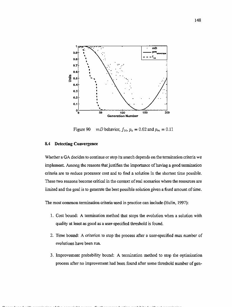
Reproduced with permission of the copyright owner. Further reproduction prohibited without permission.
1
0.9
' 0.8 • • 0.7 ' 0.6
"' 'i§ 0.5 ::1
0.4
0.3
0.2
0.1
0 0
• • 1 .. ,
'
' ' '
· mD
--pmenvelope
-- -f14
50 100 150 200 Generation Number
Figure 90 mD behavior, fr4 , Pc= 0.62 and Pm = 0.11
8.4 Detecting Convergence
148
Wh ether a GA decides to continue or stop its search depends on the termination criteria we
implement. Among the reasons thatjustifies the importance ofhaving a good termination
criteria are to reduce processor cost and to find a solution in the shortest time possible.
These two reasons become critical in the context of real scenarios where the resources are
limited and the goal is to generate the best possible solution given a fixed amount oftime.
The most common termination criteria used in practice can include (Hulin, 1997):
1. Cost bound: A termination method that stops the evolution when a solution with
quality at least as good as a user-specified threshold is found.
2. Time bound: A criterion to stop the process after a user-specified max number of
evolutions have been run.
3. lmprovement probability bound: A termination method to stop the optimization
process after no improvement had been found after sorne threshold number of gen-

Reproduced with permission of the copyright owner. Further reproduction prohibited without permission.
149
erations.
4. Convergence bound: This criterion stops the search process after the population
seems to have converged. The detection of convergence can be done by using sorne
metrics such as the standard deviation of the fitness of the population, or by measur
ing the diversity in the genomes based on sharing functions (Goldberg, 1989).
5. Loss of minimization: This criterion was proposed by Hulin (1997), and it termi
nates the GA run when the cost of additional computation exceeds the expected gain
(i.e., when the marginal utility of continuing the run is expected to be negative).
Intuitive! y, a good termination criterion stops an optimization algorithm run when a signif
icant improvement can not be expected according to the observed performance behavior of
the current run. Surprisingly, relatively little work has been done in the area of determin
ing good termination criteria (Fukunaga, 1998). In the context of our practical problem,
it could mean that we can stop the optimization process at sorne point when any future
improvement can not be significant to alter the physical response of our fly-by-wire sys
tem. So, we try, first, to implement a convergence bound criteria in our RGA by using a
Bayesian network and applying the modified Simpson's diversity index.
8.4.1 Constructing a Bayesian network for detecting convergence
To formalize and to mode! our partial reasoning and knowledge about what we know of the
behavior of out RGA using a BN, we must consider the following issues: ( 1) its domain
variables and values; (2) its structural part that encodes the causal relations among the
domain variables in the form of an acyclic, directed graph (DAG); and (3) a numerical
part that consists on the conditional probability tables for the domain variables or nodes.

Reproduced with permission of the copyright owner. Further reproduction prohibited without permission.
150
8.4.1.1 Domain variables and their values
According to (Kocis and Whiten, 1997), we need to determine which are the most impor
tant variables or nodes for our detecting convergence method among four types of nodes:
• target or query nodes which consist of those variables whose values an end-user
wants to know about,
• evidence or observation nodes that could be observed and would be useful in in
ferring the state of another variable. In other words, these nodes play the role of
sources of information about the domain,
• context variables that can be determined by considering sensing conditions and
background causal conditions, and
• controllable variables which are those whose values can be set by intervention in
the domain environment.
By following the classification described above, we identify three important variables or
nodes for our detecting method. First, because we are interested in knowing whether
an RGA has converged or not, our target variable will be named Convergence. For our
application, Convergence is a discrete node that can only have two possible states, it does
not matter if the RGA seems to converge to a local optimum or global optimum. Second,
we know that the diversity of the RGA population can give sorne kind of information about
the convergence of the algorithm; therefore, our second variable is Diversity (context
variable). For Diversity, there are four possible ordered states for describing the degree
of heterogeneity of the population: very poor, poor, moderate, and good. However, we
need a method that measures diversity by using the modified Simpson's diversity index;
thus, we will implement a method for testing diversity and the result of this method will
be the evidence variable called Test of Diversity. This last variable has also four possible

Reproduced with permission of the copyright owner. Further reproduction prohibited without permission.
151
Table XVIII
Set of Discrete Values
1 State 1 Label 1
Convergence ( C ) 1: No Cl
2: Yes C2
1: Very Poor Dl
Diversity ( D ) 2: Poor D2
3: Moderate D3
4: Good D4
1: Levell Tl
Test of Diversity ( T ) 2: Level2 T2
3: Level3 T3
4: Level4 T4
ordered states: level 1, level 2, level 3 and level 4. Table XVIII summarizes the discrete
values assigned to each one of the three variables th at are part of the BN.
To test the diversity of the population we use a window of seven values of modified Simp
son's index, mDi-6 ~ mDi-5 ~ ... ~mDi (see Figure 91 ), where i is the number of the cur
rent generation. The window is shifted along the execution of the optimization process
and handled like a FIFO structure. In the case of non-uniform mutation operator, when
diversity reduces we can have groups of zero values of mD, thus, we define four distinct
levels depending on the number of zeros that we get in the FIFO structure (Table XIX).
8.4.1.2 Graph Structure
To decide the structure of the network, we focus on the relationships between variables.
Many types of qualitative relationships can help to determine the most appropriate struc
ture for our convergence detecting problem. Among them, and very important, are the
causal relationships.

Reproduced with permission of the copyright owner. Further reproduction prohibited without permission.
152
mDi-6 mDi-5 mDi-4 mDi-3 mDi-2 mDi-1
cmTent generation -. mDi
Figure 91 FIFO structure for "Test of Diversity"
Table XIX
Levels for Test of Diversity
Symbol 1 Level 1 Number of Zeros 1
1: Level 1 5, 6, or 7
1i 2: Leve12 3 or4
3: Level3 1 or 2
4: Level4 0
To find the causal relationships in our BN, we proceed to ask direct questions about causes
(see Table XX). Th us, the Convergence of the optimization process could happen if the
Diversity is reduced to very poor levels, so, Diversity influences Convergence. We can
measure Diversity by implementing a Test of Diversity that can approximately detect
the levels of Diversity. These causal relationships can be modeled by using a Bayesian
network like the one shown in Figure 92.
By using the BN shown in Figure 92, it is possible to do bottom-up and top-down rea
sonings. This means that knowing the result of the test of diversity can help us to do a
diagnostic (bottom-up reasoning) of the state of diversity in the population of the GA.
Furthennore, when the state of diversity is obtained then we can do a causal (top-down)
reasoning of the convergence state of the GA.

Reproduced with permission of the copyright owner. Further reproduction prohibited without permission.
153
Table :XX
Finding Causal Relationships
Question Answer Modeling
What can cause Diversity
arc from Diversity to Convergence? Convergence
What can affect the results Diversity
arc from Diversity to of the Test of Diversity? Test of Diversity
Figure 92 A BN structure for detecting convergence

Reproduced with permission of the copyright owner. Further reproduction prohibited without permission.
154
8.4.1.3 Probabilities
Once we have a Bayesian network that expresses the relationship among our stochastic
variables, it is important to assign them a numerical parameter signifying the degree of
our belief accorded to them under our partial expertise and knowledge.
Table XXI describes the prior probability of Diversity (Prob( Div er s'ity) ). The values
assigned to each state reftects our belief of their presence during the optimization process.
As we can observe we expect that diversity in moderate and high levels will be present
most of the ti me during the search process of our RGA.
Table XXI
Prob( Div er s'ity)
Level 1 Probability 1
Very Poor 0.05
Poor 0.10
Moderate 0.40
Good 0.45
Table XXII shows our beliefs that a specifie lev el of Test of Diversity could happen given
sorne value of Diversity (Prob(TestO f DiversityjDiversity)). We expect that most of
the time Level 2 represents a poor diversity, Level 3 represents a moderate diversity,
and Level 4 represents a good diversity; however, it is possible to have sorne different
situations for the same level like those shown in Figure 93. As we can observe, both
examples have two zeroes, but the other values of example (a) are smaller than those of
example (b ), in fact they are very small. So, it is possible to interpret that wh ile example (a)
should be classified as a sample ofLevel3, it looks like more a Level2 sample because the
other values are very close to zero. That is why we assigned a 0.95 conditional probability
and not one.

Reproduced with permission of the copyright owner. Further reproduction prohibited without permission.
155
Table XXII
Prob(Test\Diversity)
Diversity
Very Poor Poor Modera te Good
Levell 1 0.05 0 0
Level2 0 0.95 0.05 0
Level3 0 0 0.95 0.05
Level4 0 0 0 0.95
0 0 0.05 0.71 0.05 0.65 0.08 0.68 0.08 0.68
0 0 0.05 current generation ___,. current generation --+ 0.74
(a) (b)
Figure 93 Examples of Windows for Level 3
The values in Table XXIII represent our beliefs that Convergence is or is not possible
given sorne ki nd of degree of Diversity.
Table XXIII
?rob( Con vergence\ D'iv er sity)
Diversity
Very Poor [ Poor [ Moderate j Good

Reproduced with permission of the copyright owner. Further reproduction prohibited without permission.
156
8.4.2 RGA with a dynamic termination point
Now, based on the BN that we have described above, we can implement the algorithm
of Figure 94 to in fer the probability th at the RGA converge ( C = "Y es") given th at a
level of diversity (Te) is measured by the test of diversity (Prob(C ='~Y es" ITe)). First,
the computation for the variable Te requires information determined by its parent D. This
method can be considered a message passing algorithm, in which each node passes to its
child a message needed to compute the child's probabilities (Neapolitan, 2004). Theo,
we can use upward propagation of messages to compute the conditional probabilities of
D given Te. Finally, we proceed to compute P( C = "Y es" ITe) using the downward
propagation algorithm.
1. Compute the prior probability of the leve! of evidence of the test P(Te)
4
P(Tc) == LP(TciDj)P(Dj): j=l
2. Compute the conditional probability of the diversity given the leve! of evidence of the test P(DiiTe)
for ali j = L ... , 4:
3. Compute the conditional probability of the convergence given the leve! of evidence of the test P( C == ., Y es" ITe)
4
P(C = "Yes"'ITc) = LP(C = "'Yes"IDj)P(DjiTc): j=l
Figure 94 Algorithm of inference to fi nd P( C = "Y es" ITe)
Thus, we can modify the structure of our RGA (see Figure 95) to include the possibility
of finishing the optimization process once the algorithm seems to converge to sorne value.
Whatever value of P( C = "Y es~·ITc) we obtain, we compare it with a generated random
number r, to see if we stop the optimization process or not.

Reproduced with permission of the copyright owner. Further reproduction prohibited without permission.
t- 0; initialize population(t); evaluate population(t): t = 1:
repeat {
}
select population( t) from population( t-1): apply Blend crossover to structures in population( t); apply Nonuniform mutation to structures in population(t); evaluate population(t); Determine Te Compute Prob(C = "Yes"ITe) Generate a random number r t-t+ 1:
until (r < Prob( C = "Y es" ITe) )
Figure 95 RGA with a dynamic terrnination point
8.4.3 Experiments
157
Generally for solving our practical ftight control design problem, each iteration of our
original RGA have taken 10 minutes. So, in this section, we modify our original RGA
(Figure 95) to test the new approach of finishing the optimization process. Sorne results
that correspond to cases 24, 64, 104, 124 and 144 of the ftight envelope are presented
here for analysis. For running ali our experiments, we used a Pentium IV of 3.2GHz; 1
Gigabyte of RAM, a hard disk of 80 Gigabytes, a Windows XP operating system, and we
perforrned 40 iterations for each case.
Figures 96 to 100, are the step responses of the our ftight control system simulation. Each
figure shows the step response obtained at the end of the optimization process (blue dash
dot line), and the step response that we would have obtained if the optimization process
have been stopped using our new terrnination method (green dotted line). While the step
responses obtained at generation 157 (fl5ï) and 200 (J200 ) respectively for case 124, and
generations 131 (j131 ) and 200 (j200 ) for case 24, are so similar that we do not notice any
difference between them, the other three cases have small differences, but they are still

Reproduced with permission of the copyright owner. Further reproduction prohibited without permission.
good responses.
Case24 1~~--~----,---~----~----r---~----,---~r---~---.
,.-.,, ......
... .....
F"Ç] ~
':t ! ' ~ o ef ;
·-···-·-·-·-·-·-·-·---··-·-·-·-·--·-·-·-·-··-
< 0 6
1
OAf i 0 2 1
1
1
oJ [) 2
Figure 96
l ..: 5 lj y ~0
Time(sec)
Step response for case 24
Case 64 1A;-----~--~-----T-----r----,-----,-----~----T---~~---,
1 2
~ 0.8
:ê ëi. E < 0.6
0~
0.2
0 0
1
1
'
r r
, ... · ...
......... .
2
Figure 97
-·- -·-·- -·-·-·-.. -·-·---·-·-·-·-.. -·-·-
5 Time(sec)
h 7
Step response for case 64
,, ~0
158

Reproduced with permission of the copyright owner. Further reproduction prohibited without permission.
Case104 1A~---T----~--~----~----~---T----~--~~--~----,
1.2
., 0 8
~ a. E < 0 6
02
1
1
1 ,, " ,, ... ... ,,
0~--~----~----~--~----~----~----~--~----~----~ Q r' 5 H 0
Tlme(sec)
Figure 98 Step response for case 104
Case124 1 -:~--~~--~-----r----~----~----,-----~----r---~----~
1 2
~ 0 H
~ a. E < Oci
0 2 ' 1
1
1
, " 1
... ... , -- -- -·- -- -·-·--·-·--·-·--·-·--·-·--·-·-
OAI [
0o~----~----~----~3----~----~s----~6----~~--~e----~9----~,o
Tlme (sec)
Figure 99 Step response for case 124
159

Reproduced with permission of the copyright owner. Further reproduction prohibited without permission.
''f / ,\_ 1 1
1
!).:
~.~~-----------------------
3 s Tlme (sec)
Figure 100 Step response for case 144
160
1 îO
Table XXIV summarizes the results obtained for each of the cases that we tested. It is
possible to observe that in the worst average case we need around 152 generations to have
a good step response from our simulation madel. This means that we can have good results
at seven and half minutes of optimization process instead of 10 minutes, a saving of two
and half minutes.
Table XXIV
Statistics of termination points using non uniform mutation
1 Case Average Std. Dev. 1
24 142 6.3
44 143 6.7
64 139 12
84 139 Il
104 137 21
124 152 9.7
144 143 18

Reproduced with permission of the copyright owner. Further reproduction prohibited without permission.
161
8.5 Detecting stages of optimization
Li et al. ( 1992) suggest that the optimization process of a GA involves three stages named:
initiation, search and refinement. In the initial stage, diversity measures depend on the ini
tial conditions of the GA, so the diversity measure's behavior is unpredictable and control
parameters should be kept constant. The search stage, should guarantee a broad search
and efficient exploitation; therefore. control parameters have to be designed to vary ade
quately. Finally, in the last stage, refinement, control parameter values should be balanced
in a way that we increase the exploitation and the search is forced in local regions.
If we observe the envelope of the nonuniform mutation, we can notice that this mutation
operator follows very close the suggestion of Li et al. ( 1992). However, one can argue that
because of the dynamic behavior of the optimization process it is possible that there were
more than three stages, specially where there is a transition between the first and second
stage, and between the second and third stage. Therefore, besides knowing in which stage
the GA is, it is also very important to know when each stage begins and when it ends, or
in other words, where each transition happens.
To detect these transitions we propose to use our new Bayes Network to detect the conver
gence of the optimization process at different levels of E, which is the accuracy factor of
the first class in Table XVII. The idea behind this heuristic is that when we use a nonuni
form mutation operator, we observe that the RGA gets close to the global optimum region
or in the worst case to a local optimum region at different levels of precision. By setting
up different values forE, we can define different set of levels for the computation of mD.
Then, when our BN detects convergence it will be the moment where another stage will
take place and we will have to change the value of E in order to go for another stage.
For our design's purposes we will considera set of four values forE such as we can detect
four stages instead of three: initiation, search, medium search and refinement.

Reproduced with permission of the copyright owner. Further reproduction prohibited without permission.
162
8.5.1 Adaptive Nonuniform Mutation Operator
Once we have a new method for determining different stages of the optimization process
we can try to adapt the envelope of the nonuniform mutation operator. The idea here is
twofold: first, nonuniform mutation has a very weil defined envelope, but this envelope is
very related with three clear stages of the optimization process, in other words, it follows
very strictly the suggestion of Li et al. ( 1992); and second, the results of Chapter 6 showed
that in general periodic mutation operator had better performance than nonuniform mu
tation operator when both were applied to the problem of Bombardier, so, the adaptation
of the nonuniform mutation operator could improve its performance versus the periodic
mutation.
Basically, the value of the mutation probability of the nonuniform mutation changes ac
cording to the ratio of the current generation t over the total number of generations to be
ran T. AsTis constant during the who le process, we will adapt the value of t, which will
be named tadaptive· Generally, tadaptive will be constant, but it will change to be equal to
the current t if there is a change to another stage of optimization process, and/or if there
has not been new optimal values during the last five generations. The intuition behind the
second criteria is that if tadaptive is constant for sorne generations and there is not more
new optimization values then it is likely that it has become ineffective. The value of five
was chosen after several tests with mathematical functions. It was found that there was not
big difference of performance comparing with 10 and 15. However, the performance of
the algorithm degraded significatively when we used values greater than 15. Besides, we
considered that five was a better choice keeping in mi nd that we only have 200 generations
to the whole optimization.
Figure 101 shows the new method for implementing the adaptive nonuniform mutation,
and Figure 102 includes the new method for adapting the nonuniform mutation operator
and for stopping the optimization process to the base architecture of GA, and we named

Reproduced with permission of the copyright owner. Further reproduction prohibited without permission.
this new structure a Probabilistic Adaptive Genetic Algorithm.
function [flag. tadaptztoe• é] = Adaptive(flag, t, tadaptire• é. ?rob( C =··Y es" !Te))
Generate a random number r:
if r < ?rob( C = ··Y es" ITe) then if é < 0.0001 then
tadaptit•e = t:
é = é * 0.1: else
flag = false: end
end
Figure 101 Adaptive Nonuniform Mutation Algorithm
t- 0; initialize population(t): evaluate population(t): t = 1: é = 0.1: flag = true: tadaptive = t;
repeat {
}
Select population(t) from population(t-1); apply Blend crossover to structures in population(t): apply Nonuniform mutation using tadaptive to structures in population(t): Evaluate population(t); Determine Te Compute Prob(C = "Yes''ITc) [flag, tadaptive. c] = Adaptive(Jlag. t. tadaptive. c, Prob(C = ··ves''ITe)) if there have not been optimization during the la:;t five generations then
tadaptive = t: end t-t+ 1:
until (Jlag is false)
Figure 102 Probabilistic Adaptive Genetic Algorithm
163
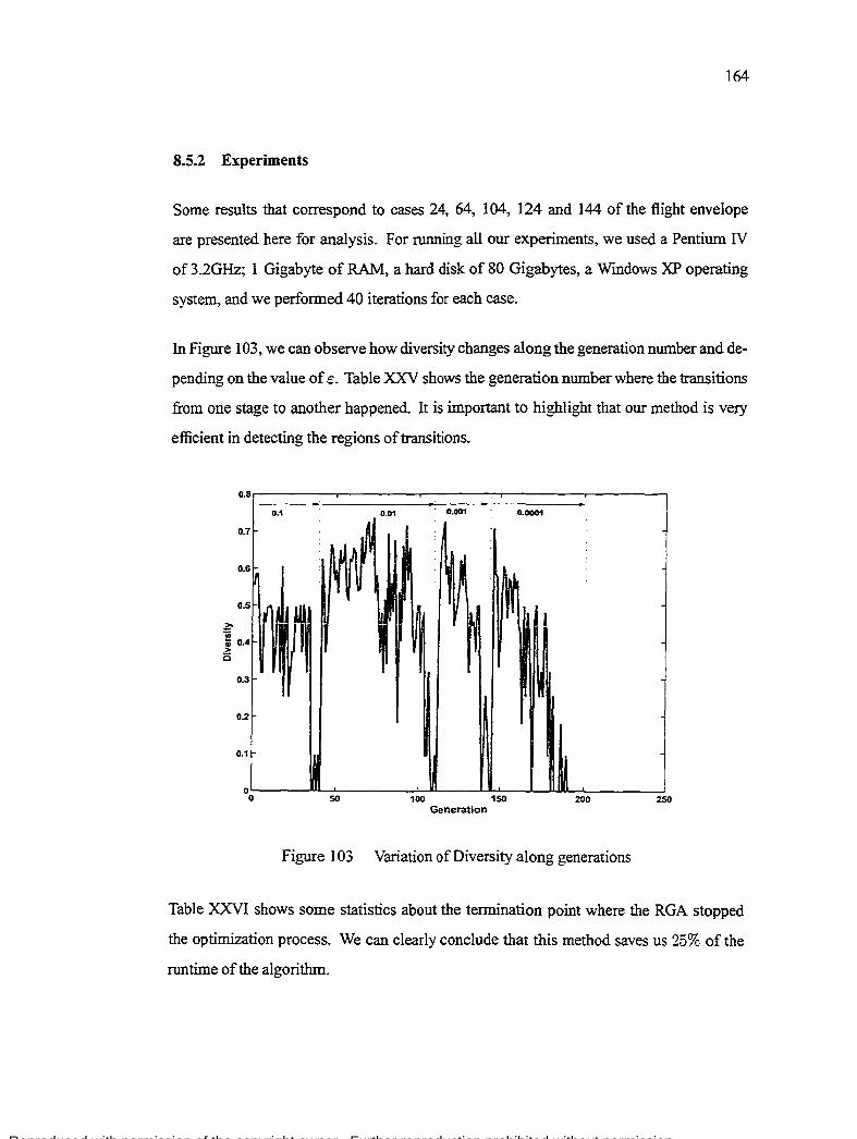
Reproduced with permission of the copyright owner. Further reproduction prohibited without permission.
164
8.5.2 Experiments
Sorne results that correspond to cases 24, 64, 104, 124 and 144 of the ftight envelope
are presented here for analysis. For running all our experiments, we used a Pentium IV
of 3.2GHz; 1 Gigabyte of RAM, a hard disk of 80 Gigabytes, a Wmdows XP operating
system, and we performed 40 iterations for each case.
In Figure 103, we can observe how diversity changes along the generation number and de
pending on the value of c. Table XXV shows the generation number where the transitions
from one stage to another happened. It is important to highlight that our method is very
efficient in detecting the regions of transitions.
0.8 -0.1 0.01 0.001 0.11001
0.7
~ ~ 0.6
~ 0.5 ~r 2:' jjj <; 0.4 ~~ > ë
0.3
0.2
0.1 1 l 0o~----~-~~-------1~oo_u----~1~~---L~BL~2o~o------~~
Generation
Figure 103 Variation of Diversity along generations
Table XXVI shows sorne statistics about the termination point where the RGA stopped
the optirnization process. We can clearly conclude that this method saves us 25% of the
runtime of the algorithm.

Reproduced with permission of the copyright owner. Further reproduction prohibited without permission.
165
Table XXV
Change of~
\ Generation c\ 0.1
40 0.01
110 0.001
144 0.0001
Table XXVI
Statistics about tennination point of GA
Case Average Std. Dev. Minimum Maximum 1
24 137 9.0 121 153
44 141 10.0 125 156
64 140 4.9 133 150
84 144 10.0 128 160
104 147 8.2 136 160
124 150 7.2 136 164
144 149 8.9 135 162
Table XXVII and XXVIII demonstrate that the difference of the results obtained by using
our tennination method (xf, F) are close in tenns of distance and cost to the results that
were produced by letting the algorithm run 200 generations (xf00 ' j2°0).
Figures 104 to 108, are our simulation model. Each figure shows the step response ob
tained at the end of the optimization process (blue dash-dot line), and the step response
that we would have obtained if the optimization process have been stopped using our new
termination method (red dotted line). Except for the case 64 where both responses show
little differences. the responses for ali the ether cases are so similar that we do not notice
any difference between them. If we compare these results with those obtained using the

Reproduced with permission of the copyright owner. Further reproduction prohibited without permission.
166
original nonuniform mutation operator, we verify that these are better.
Table XXVII
Statistics of the differences for the best results
1 Index L:- ( "' ·JOOf v x~- x-:- -1=1 t 1.
r _ 12oo
Average 0.01492 0.00009
Standard Deviation 0.01335 0.00007
Minimum 0.00287 0.00002
Maximum 0.03901 0.00018
Table XXVIII
Statistics of the difference for ali the results
1 Index L:'?_ x~- x-:- -- ( "' ·JOOf 7.-l 1 1
g _ jpoo j
Average 0.01663 0.00016
Standard Deviation 0.01172 0.00013
Minimum 0.00134 0.00001
Maximum 0.05358 0.00070
Figures 1 04 to 1 08, are our simulation model. Each figure shows the step response ob
tained at the end of the optimization process (blue dash-dot line), and the step response
that we would have obtained if the optimization process have been stopped using our new
termination method (red dotted line). Except for the case 64 where both responses show
little differences, the responses for ali the ether cases are so similar that we do not notice
any difference between them. If we compare these results with those obtained using the
original nonuniform mutation operator, we verify that these are better.
Although the differences in the performance among the nonuniform mutation, periodic
mutation and adaptive nonuniform mutation operators are not so remarkable, Figures 109

Reproduced with permission of the copyright owner. Further reproduction prohibited without permission.
Case24 -:.4
:.2 ,~
/~ i .. '
--------j i !
0 08 i "0
1 ~ 0:.
1 E < OG
0."
0.~
0
1 2
«» O.H
~ 0:. E <C O.tJ
o . .:
02
0
i ! j 1
1 1
! i
1
oLL
1
• ' 1
3 .: •i Time(sec)
Figure 104 Step response for case 24
Case64
.' ... ....
· ....
-·. -·.·-'- ·-···- ·- ·- 0 -·-.. ·-·-· -·- .. ·-···-·-' -·- ··-·-
2 8 Time(sec)
Figure 105 Step response for case 64
167

Reproduced with permission of the copyright owner. Further reproduction prohibited without permission.
Case104 14r----r----T---~----~----r----r----~--~----~----,
1.2
.. 0 ~ ~ 0
ë. E < 0 G
0-'
0.2
1
1 , ·----.... .....
~.
. '"··-·-. -·-···- ··-·-. -·-· ·-·-. -·-···-··- ·-. -·- .. -·-
0 uLL~--~----~----~-----L ____ _. ____ _. ____ _. ____ _. ____ ~----~ 0 L) 5 8 ~0
Time(sec)
Figure 106 Step response for case 104
Case124 1 ·•r---~~--~-----r-----r----~----~----~----r-----~---,
1 2
~ O.H ,g ë. E < O.n
02
...... 1 ·,
, " , ' 1
' " " "
.... _,_,_ -·- -·- -·--·- -- -·-·-·--- -·--·-·-·--
0o~----L-----~----3~-----4.----~----~----~----_.8----~9~--~,o
Tlme(sec)
Figure 107 Step response for case 124
168

Reproduced with permission of the copyright owner. Further reproduction prohibited without permission.
''[ 1::
0.08
0.07
0.06
o.os .. 0 u .,
0.114 "' ~ > < 0.03
0.02
0.01
case144
/'\ ~ ] '·,·--·- ------------------------ j
Time(sec)
Figure 108 Step response for case 144
~
',. , ......... ~ ' ',
, , '
·~
' ... , ' ,'
1
. • . Adaptt".re 1 J ·. e · Non-unlform +· Per'.odlc
' '"· ~, .. ,, .... - ,, --....... , '
•
- -: ..... •., ' , \~- ~""' , · ........... 'ô ..,_ ; """" ~-' ..... _. __ ... -
1114 124
Case number
j
144
Figure 109 Cost Average using Adaptive Nonuniforrn Mutation
169

Reproduced with permission of the copyright owner. Further reproduction prohibited without permission.
170
and 110 show that by including our Bayes Network in the original nonuniform mutation
in order to control Pm we were able to improve its performance and compete with the pe
riodic mutation operator.
13
12
11
Il
7
6
5
"'
' ; 1 • t
• • .'!. • ~
.-- :-:' \ '1-~
Cost
"' /•\ /~\ 1! ~ \
f/ \':,
1 ···~ 1 • Non-untfonn • Periodlç
• "
\ ,, 1! \ ', J 1 '',
Il
Il
1 1
1 1
1 1
1 1 "'1 1
•
24
"' "' ,, ,, ·~· ·, ..
, 1 '' ' . ' J ! '· \\ , 1 '\ ' . \
, 1 '\ 1 \
1 1 \\ ' . \ ~ ! \\ \
, 1 '\ '. \ , 1 \\
'~ ,', ,_,\ , ,,_ /1 ' ... '" / ; ,', ,- - -. -\1:1 i . , - .:-~: ,+; \-
v • \ ,· --·-·-·-···'
114 104 12-4 Casenumber
1-44
Figure 110 Standard Deviation using Adaptive Nonuniform Mutation
The controller gain values for all 160 cases of Bombardier by using the stopping point as
well as by using 200 generations are registered in Appendices 4 and 5 respectively.

Reproduced with permission of the copyright owner. Further reproduction prohibited without permission.
CONCLUSION
The overriding goal to accomplish in this research was to seek the improvement of the
performance of Genetic Algorithms in order to be applied effectively and efficiently to
the optimization of controller gains of a fly-by-wire system. By effectively, we mean
that any solution produced by our improved GA should fall very close to the real global
optimum (small standard deviation) independently of how often the GA is invoked. And,
by effi.ciently, we mean that our improved GA should resolve the problem in a shorter ti me
(small cpu time) than the classical GA without affecting its effectiveness.
In order to target the first part of our goal, a new mutation operator was irnplernented.
We succeeded in combining the characteristics of two mutation operators. uniform and
nonuniform, in a new one, periodic, and to get controllers that generate the smallest min
imal cost for the eight cases, with a more stable and smaller mean and standard deviation
than the uniform and nonuniform mutation operators using a maximum of two hundred
generations. However, using a deterministic parameter control technique on the design of
the periodic mutation operator did not save us from the process of manual tuning, but it
did improve the effectiveness of our GA in the aircraft control design problern.
The effectiveness in solving a real optimization problem also depends on the accuracy
of the model used to implement the objective function. While the unconstrained model
provided by Bombardier includes the handling quality criteria that have to be satisfied ac
cording to requirements of regulators, it does not have a direct way of controlling its step
response. Thus, our proposed constrained mode] and the implementation of the new con
strained stochastic tournament selection operator increased the effectiveness of a RGA by
generating better step responses than the unconstrained model and satisfying at the same
time the handling quality criteria of the system. Besides satisfying the handling qualities
criteria, this model contributes to the designer with a flexible way of controlling the char-

Reproduced with permission of the copyright owner. Further reproduction prohibited without permission.
172
acteristics of the step response of the system. For the implementation of the constrained
stochastic toumament selection, the key idea was to implement a method that can han
die the proportion of feasible and unfeasible individuals without neglecting the dynamic
behavior of GAs.
Though computation time is not significant in the case of an optimization of numerical
functions, it is very important when we use simulation of real engineering problems to
evaluate the objective function. Trying to measure the dissimilarity of the genes in a pop
ulation during the optimization process of Real-Coded GAs that use mutation operators
with decreasing mutation policies, showed that there exists a set of classes of chromo
somes around the best individual with sorne characteristics that their diversity becomes
critical for detecting convergence. The results also showed that when the modified Simp
son 's index was below sorne value KmD then the likelihood that convergence happened
was very high. Thus, by combining the use of mD together with a Bayes Network, we
were able to introduce our partial knowledge and expertise to detect convergence and to
stop the optimization process, saving sorne computation time, and reaching the second
part of our research goal, improved efficiency.
The use of mD and the Bayes Network was key for the implementation of the new Prob
abilistic Adaptive Genetic Algorithm. While we considered that adapting the nonuniform
mutation operator is not the best that we can do using mD and our BN, it shows without
difficulties the way to improve sorne already existing mutation operator. However, more
work remains to be made.
Three were the key ideas that lead this research, first, keep simple any improvement to
the RGA. It is already difficult to analyze a complex system like a Genetic Algorithm.
Second, do a thoughtful analysis and application of heuristics, and partial knowledge and
expertise that we have or we get. And, third, do a careful experimentation to test the new
methods.

Reproduced with permission of the copyright owner. Further reproduction prohibited without permission.
RECOMMENDATIONS
In this final chapter we suggest a number of potential continuations of the work described
in this dissertation.
It will be very important to know if the modified Simpson 's index can be applied to dif
ferent architectures of RCGAs. By different architectures, we intend to refer to different
types of crossover and mutation operators. Another work that remains to be done is to see
if the index using a different set of classes can permit to know with more precision the
behavior of the RCGAs at different stages others than the last one.
It will be very interesting and useful to find a mathematical model that relates, e with the
precision of the final results. The idea is that with an exact or very close model it will be
possible to know orto control the precision of any solution of the RGA.
By following the guidelines of the methodology used in this research, it is important to
see the possibility of extending the use of the mo di fied Simpson 's index and the Bayes
network for controlling the dynamic behavior of the crossover operator.
Another extension of this research should be the use of Bayes Network and a diversity
index similar to the one used in this research, to improve the performance of RGA for
solving constrained optimization problems. A good candidate to be a variable of the BN
should be the ratio of feasible and unfeasible individuals of the generation along the opti
mization process.
While this research has shown the use of Bayes Network and a diversity index to RGA, it
remains to try their use with GAs of different encoding such as binary and integer.

Reproduced with permission of the copyright owner. Further reproduction prohibited without permission.
APPENDIX 1
UNCONSTRAINED TEST FUNCTIONS

Reproduced with permission of the copyright owner. Further reproduction prohibited without permission.
175
De J ong function 1
De Jong's function 1 is a simple function. It is continuo, convex and unimodal. Its defini
tion is:
n
JI(x) =:Lx~ (8.14) i=l
where -5.12 :s; xi :s; 5.12, and its global minimum is at xi = 0 for i = 1 · · · n and j 1 = O.
Rosenbrock valley (De Jong's function 2)
Rosenbrock's valley is a classic optimization problem, also known as Banana function.
The global optimum is inside a long, narrow, parabolic shaped flat valley. To find the
valley is trivial, however convergence to the global optimum is difficult and hence this
problem has been repeatedly used in assess the performance of optimization algorithms.
Its function definition is:
n-l
h(x) = L 100(xi+l- x~?+ (1- x1f (8.15) i=l
where -2.048 :s; x; :s; 2.048, and its global minimum is at xi = 1 for i = 1 · · · n with
h(x) =O.
First Rastrigin function
Rastrigin's function is based on function 1 with the addition of eosine modulation to pro
duce many local minima. Thus, the test function is highly multimodal. However, the
location of the minima are regularly distributed. Its function definition is:

Reproduced with permission of the copyright owner. Further reproduction prohibited without permission.
176
n
h(x) =lOn+ LXT -lOcos(2JTx1) (8.16) i=l
where -5.12 ~ Xi < 5.12, and its global minimum is at Xi = 0 for i = 1· · · n with
h(x) =O.
Schwefel function
Schwefel function is deceptive in that the global minimum is geometrically distant, over
the parameter space, from the next best local minima. Therefore, the search algorithms
are potentially prone to convergence in the wrong direction. Its function definition is:
n
j4(x) = L -x1sin(vTxJ) (8.17)
i=l
where -500 ~ Xi ~ 500, and its global minimum is at xi = 420.9687 for i = 1 · · · n with
j4(x) = -418.9829n.
Griewangk function
Minimize:
n •)
fo(x) = L 4~~0 - II cos( x~)+ 1 i=l vz
(8.18)
where -600 < Xi < 600, and its global minimum is at Xi - 0 for i - 1 · · · n with
fo(x) =O.
Sum of different power function
Minimize:

Reproduced with permission of the copyright owner. Further reproduction prohibited without permission.
177
(8.19)
where -1 :S Xi :S 1, and its global minimum is at Xi = 0 for i = 1 · · · n with f 6 (x) = O.
Ackley path function
Minimize:
b IL. x; 2 L cos(cx;)
h(x) = -ae- v n - e Tl +a+ e (8.20)
where a = 20, b = 0.2, c = 27ï, -32.768 :S xi :S 32.768. The function has a global
minimum value of 0 at xi = 0 for i = 1. · · · n.
Michalewicz function
Minimize:
(8.21)
where 0 :S x1 :S 7ï. The function has several global minimum values of -4.687 at different
locations.
Langermann function
Minimize:
rn
fg(x) = L cie-~cos(d7ï) (8.22) i=l

Reproduced with permission of the copyright owner. Further reproduction prohibited without permission.
178
where
n
d = I)xi- ai)2 (8.23)
i=l
( 0.806 0.517 1.5 0.908 0.965 0.669 0.524 0.902 ... ) 0.531 0.876 0.462 0.491 0.463 0.714 0.352 0.869 ... c = 0.813 0.811 0.828 0.964 0.789 0.360 0.369 0.992
0.332 0.817 0.632 0.883 0.608 0.326
9.681 0.667 4.783 9.095 3.517 9.325 6.544 0.211 5.122 2.020 9.400 2.041 3.788 7.931 2.882 2.672 3.568 1.284 7.033 7.374 8.025 9.152 5.114 7.621 4.564 4.711 2.996 6.126 0.734 4.982 2.196 0.415 5.649 6.979 9 .. 510 9.166 6.304 6.054 9.377 1.426 8.074 8.777 3.467 1.863 6.708 6.349 4.534 0.276 7.633 1.567 7.650 5.658 0.720 2.764 3.278 5.283 7.474 6.274 1.409 8.208 1.256 3.605 8.623 6.905 0.584 8.133 6.071 6.888 4.187 5.448 8.314 2.261 4.224 1.781 4.124 0.932 8.129 8.658 1.208 5.762 0.226 8.858 1.420 0.945 1.622 4.698 6.228 9.096 0.972 7.637 7.305 2.228 1.242 5.928 9.133 1.826 4.060 5.204 8.713 8.247 0.652 7.027 0.508 4.876 8.807 4.632 5.808 6.937 3.291 7.016 2.699 3.516 5.874 4.119 4.461 7.496 8.817 0.690 6.593 9.789 8.327 3.897 2.017 9 .. 570 9.825 1.150 1.395 3.88.5 6.354 0.109 2.132 7.006 7.136 2.641 1.882 5.943 7.273 7.691 2.880 0.564 4.707 5.579 4.080 0.581 9.698 8.542 8.077 8.515 9.231 4.670 a= 8.304 7 . .559 8.567 0.322 7.128 8.392 1.472 8.524 2.277 7.826 8.632 4.409 4.832 5.768 7.050 6.715 1.711 4.323 4.405 4.591 4.887 9.112 0.170 8.967 9.693 9.867 7.508 7.770 8.382 6.740 2.440 6.686 4.299 1.007 7.008 1.427 9.398 8.480 9.950 1.675 6.306 8.583 6.084 1.138 4.350 3.134 7.853 6.061 7.4.57 2.2.58 0.652 2.343 1.370 0.821 1.310 1.06:3 0.689 8.819 8.8:33 9.070 5.558 1.272 5.756 9.857 2.279 2.764 1.284 1.677 1.244 1.234 3.352 7.549 9.817 9.437 8.687 4.167 2.570 6.540 0.228 0.027 8.798 0.880 2.370 0.168 1.701 3.680 1.231 2.390 2.499 0.064 1.460 8.057 1.336 7.217 7.914 3.615 9.981 9.198 5.292 1.224 0.432 8.645 8.774 0.249 8.081 7.461 4.416 0.652 4.002 4.644 0.679 2.800 5.523 3.049 2.968 7.225 6.730 4.199 9.614 9.229 4.263 1.074 7.286 5.599 8.291 5.200 9.214 8.272 4.398 4.506 9.496 4.830 3.150 8.270 5.079 1.231 5.731 9.494 1.883 9.732 4.138 2.562 2.532 9.661 5.611 5.500 6.886 2.341 9.699 6.500

Reproduced with permission of the copyright owner. Further reproduction prohibited without permission.
179
0 ~ Xi ~ 10 and its global minimum f 9 (x) = -1.4 for m = 5.
Branin RCOS function
Minimize:
where -5 ~ x 1 ~ 10 and 0 ~ x2 ~ 15. The function has a global minimum value
of fro = 0.397887 at three different points: (x1 , x2 ) = ( -11, 12.275), (11, 2.275), and
(9.42478, 2.475).
Easom function
Minimize:
(8.25)
where -100 ~Xi~ 100 and its global minimum is at xi= 7ï for i = 1, 2 with fn(x) =
-1.
Goldstein-Price function
Minimize:
!r2(x) =[1 + (x1 + Xz + 1)2(19- 14xl + 3xî- 14x2
+ 6x1x2 + 3x~)][30 + (2x1 - 3x2f(18
- 32xl + 12xî + 48x2- 36xlx2 + 27xz.2)]
(8.26)

Reproduced with permission of the copyright owner. Further reproduction prohibited without permission.
180
where -2:::; Xi:::; 2 and its global minimum is at (0, -1) with f 12 (x) = 3.
Six-hump camel back fonction
Minimize:
(8.27)
where -3 :::; x1 :::; 3 and -2 :::; x2 :::; 2. The function has a global minimum value of
-1.0316 at two different point: (xl. x2) = (-0.0898, 0.7126), (0.0898, -0.7126).
Second Rastrigin function
Minimize:
1 ~( 4 •) ) h4(x) =?+~xi- 16xj + 5xi (8.28) - i=l
where -10:::; Xi :::; 10 and its global minimum is at xi = 0 for i = 1· · · n with f 14 (x) =
o.

Reproduced with permission of the copyright owner. Further reproduction prohibited without permission.
APPENDIX2
NONLINEAR CONSTRAINED TEST FUNCTIONS

Reproduced with permission of the copyright owner. Further reproduction prohibited without permission.
182
The GA community has used several nonlinear constrained optimization problems for
testing different implementations of GAs. Michalewicz (1995) suggested sorne impor
tant characteristics to be considered for the selection process of a suitable set of difficult
problems for nonlinear constrained optimization:
a. the type of the objective function,
b. the number of variables,
c. the number of constraints,
d. the types of constraints,
e. the number of active constraints at the optimum,
f. the ratio p between the sizes of the feasible search space and the whole search space
1.r n SI/ISI.
By following the guidel ines above mentioned, Michalewicz ( 1996) and Koziel and Michalewicz
(1999) proposed a set of eleven functions (see below), which were used in the experi
ments reported by the articles analyzed in this work. This set included linear, quadratic,
cubic, polynomial and nonlinear objective functions with various numbers of variables,
and different types (linear inequalities, nonlinear equations and inequalities) and numbers
of constraints.
Table XXIX summarizes the characteristics of these test cases, such as the nu rn ber of vari
ables (n), the type of function (j), the relative size of the feasible region in the search
space given by a ratio (p), the number of constraints in each category (linear inequalities
LI, nonlinear equations NE and inequalities N !), and the number N AC of active con
straints at the optimum. Koziel and Michalewicz (1999) describe that the ratio p = 1 1~/ was
determined experimentally by generating 1,000,000 random points from Sand checking
whether they belong to .r.
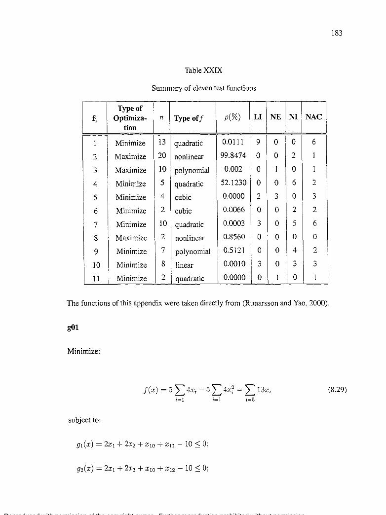
Reproduced with permission of the copyright owner. Further reproduction prohibited without permission.
183
Table XXIX
Summary of eleven test functions
Type of fi Optimiza- n Type off p(%) LI NE NI NAC
ti on
1 Minimize 13 quadratic 0.0111 9 0 0 6
2 Maximize 20 nonlinear 99.8474 0 0 2 1
.... Maxim ize 10 polynomial 0.002 0 1 0 1 _,
4 Minimize 5 quadratic 52.1230 0 0 6 2
5 Minimize 4 cu bic 0.0000 2 .... 0 ... _, _,
6 Minimize 2 cu bic 0.0066 0 0 2 2
7 Minimize 10 quadratic 0.0003 ... 0 5 6 _,
8 Maxim ize 2 nonlinear 0.8560 0 0 0 0
9 Minimize 7 polynomial 0.5121 0 0 4 2
10 Minimize 8 linear 0.0010 3 0 ... ... _, _,
11 Minimize 2 quadratic 0.0000 0 1 0 1
The functions of this appendix were taken direct! y from (Runarsson and Yao, 2000).
gOl
Minimize:
f(x) = 5L4xi -5:L4xf- Ll3xi (8.29) i=l i=l i=5
subject to:
9I(x) = 2xl + 2x2 + xw + xn - 10 ~ 0;
92(x) = 2xl + 2x3 + xw + X12- 10 ~ 0;

Reproduced with permission of the copyright owner. Further reproduction prohibited without permission.
184
95(x) = -8x2 + Xn ::; 0;
9s(x) = -2x6- Xï + x11 ::; 0;
9g(x) = -2xs- Xg + x12 ::; 0;
where the bounds are 0 ::; Xi ::; 1 ('i = 1, 0 0 0, 9), 0 ::; xi ::; 100 (i = 10, 11, 12) and
0 ::; x 13 ::; 1. The global minimum is at x* = (1, 1, 1, 1, 1, 1, 1, 1, 1, 3, 3, 3, 1) where six
constraints are active (91, 92, 93, 9ï, 9s and 99) and f(x*) = -15°
g02
Maximize:
J"'"'n o ·)
L..i=1 'lXj
(8030)
subject to:
91 (x) = oo75 - rr~::1 Xi ::; o:

Reproduced with permission of the copyright owner. Further reproduction prohibited without permission.
185
92(x) = 2:::~= 1 Xi- 7.5n::; 0;
where n = 20 and 0 ~ Xi ~ 10 (i = 1, ... , n). The global maximum is unknown,
the best that has been found is f(x*) = 0.803619, constraint g1 is close to being active
Cg1 = -10-8).
g03
Maximize:
n
J(x) = ( Vn)n II Xi;
i=1
subject to:
where n = 10 and 0 ~ Xi ~ 1 (i = L ... , n). The global minimum is at xj
(i = 1, ... , n) where f(x*) = L
g04
Minimize:
(8.31)
1 -vn
f(x) = 5.3578547x~ + 0.835689lx1x5 + 37.29:3239x1 - 40792.141: (8.32)
subject to:

Reproduced with permission of the copyright owner. Further reproduction prohibited without permission.
186
g1(x) = 85.334407 + 0.0056858x2x5 + 0.0006262x1x4 - 0.0022053x3x5 - 92 ~ 0;
g2(x) = -85.334407- 0.0056858x2xs- 0.0006262x1x4 + 0.0022053x3x5 ~ 0;
g3(x) = 80.51249 + 0.0071317x2x5 + 0.0029955x1x2 + 0.0021813x~- 110 ~ 0;
g4 (x) = -80.51249- 0.0071317x2x5- 0.0029955x1x2 - 0.0021813x~ + 90 ~ 0;
g5(x) = 9.300961 + 0.0047026x3x5 + 0.0012547x1x3 + 0.0019085x3x4- 25 ~ 0:
g6 (x) = -9.300961- 0.0047026x3x5 - 0.0012547x1x3 - 0.0019085x3x4 + 20 ~ 0:
where 78 ~ x1 ~ 102, :33 ~ x 2 ~ 45, and 27 ~ Xi ~ 45 ('i = 3, 4, 5). The opti
mum solution is x* = (78, 33,29.995256025682,45, 36.775812905788) where f(x"') = -30665.539. Two constraints are active (g1 and g6).
gOS
Minimize:
( . 3 0.000002 3
j x)= 3x1 + 0.000001x1 + 2x2 + 3
x 2: (8.33)
subject to:
h3 (x) = 1000sin( -x3 - 0.25) + 1000sin( -x4 - 0.25) + 894.8- x1 = 0;

Reproduced with permission of the copyright owner. Further reproduction prohibited without permission.
187
h4 (x) = 1000sin(x3- 0.25) + 1000sin(x3 - x4 - 0.25) + 894.8- x2 = 0;
h5(x) = 1000sin(x4- 0.25) + 1000sin(x4- X3- 0.25) + 1294.8 = 0;
where 0 ::; x 1 ::; 1200, 0 ::; x2 ::; 1200, -0.55 ::; X3 ::; 0.55 and -0.55 ::; x4 ::; 0.55.
The best known solution is x"' = (679.9453, 1026.067,0.1188764, -0.3962336) where
f(x"') = 5126.4981 (Koziel and Michalewicz, 1999).
g06
Minimize:
(8.34)
subject to:
where 13 ::; x 1 ::; 100, and 0 ::; x2 ::; 100. The optimum solution is x· = (14.095, 0.84296)
where j(x*) = -6961.81388. Both constraints are active.
g07
Minimize:

Reproduced with permission of the copyright owner. Further reproduction prohibited without permission.
188
f(x) = xî +x~+ x1x2- 14xl - l6x2 + (x3- 10)2 + 4(x4 - 5f
+ (x5 - 3)2 + 2(x6- 1)2 + 5x~ + 7(xs- llf + 2(x9 - lOf (8.35)
+ (x10- 7)2 + 45;
subject to:
9I(x) = -105 + 4x1 + Sx2- 3xï + 9xs:::; 0;
93(x) = -8x1 + 2x2 + 5xg- 2x10 - 12 :::; 0;
94 (x) = 3(x1 - 2) 2 + 4(x2- 3)2 + 2x~- 7x4 - 120:::; 0:
95(x) = 5xî + 8x2 + (x3- 6)2- 2x4 - 40:::; 0;
9;(x) = 0.5(x1 - 8)2 + 2(x2- 4)2 + 3x~- x6 - 30:::; 0:
9s(x) = -3x1 + 6x2 + 12(xg- 8)2- 7x10 :::; 0:
where -10 :::; x1 :::; 10 ('i = 1, ... , 10). The optimum solution is x* = (2.171996,
2.363683, 8.773926,.5.095984, 0.9906.548, 1.4:30574, 1.321644, 9.828726,8.280092, 8.375927)
where f(x*) = 24.3062091. Six constraints are active (91, 92, 9:h g4, 95 and 96).
g08
Maximize:

Reproduced with permission of the copyright owner. Further reproduction prohibited without permission.
subject to:
f(x) = sin3(2:x 1)sin(2JTx2 );
x1(xl +x2)
189
(8.36)
where 0 ::; x 1 ::; 10, and 0 ::; x 2 ::; 10. The optimum is located at x* = (1.2279713,
4.2453733) where f(x") = 0.095825. The solution lies within the feasible region.
g09
Minimize:
(8.37)
subject to:
9l(x) = -127 + 2xf + 3x~ + X3 + 4x~ + 5x5 ::; 0:
93(x) = -196 + 23x1 +x§+ 6x~- 8x;::; 0;
where -10::; xi::; 10 (i = 1, ... , 7). The optimum solution is x*= (2.330499, 1.951:372,

Reproduced with permission of the copyright owner. Further reproduction prohibited without permission.
190
-0.4775414, 4.365726, -0.6244870, 1.038131, 1594227) where f(x*) = 680.6300573.
Two constraints are active (g1, and 94 ).
glO
Minimize:
f(x) = x1 + x2 + x3; (8.38)
subject to:
g1(x) = -1 + 0.0025(x4 + x6)::; 0;
93(x) = -1 + 0.01(xs- xs) ::; 0;
94(x) = -x1x6 + 833.33252x4 + 100x1- 83333.333::; 0;
96(x) = -x3xs + 1250000 + X3X5- 2500xs::; 0;
where 100 ::; x1 ::; 10000, 1000 ::; Xi ::; 10000 (i = 2, 3) and 10 ::; Xi ::; 1000
(i = 4, ... , 8). The optimum solution is x* = (579.3167, 13.59.943, 5110.071, 182.0174,
295.5985, 217.9799, 286.4162, 395.5979) where f(x•) = 7049.3307. Three constraints
are active (g1, 92 and 93).
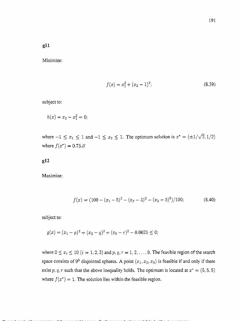
Reproduced with permission of the copyright owner. Further reproduction prohibited without permission.
191
gll
Minimize:
j (X) = xî + ( X2 - 1 f (8.39)
subject to:
where -1 ~ x 1 ~ 1 and -1 ~ x 2 ~ 1. The optimum solution is x"'= (±1/v'2, 1/2)
where f(x*) = 0.75.//
g12
Maxim ize:
subject to:
g(x) =(xl- pf + (x2- qf + (x3- rf- 0.0625 ~ 0;
where 0 ~xi~ 10 (i = 1. 2, 3) andp, q, r = 1, 2, ... , 9. The feasible region of the search
space consists of 93 disjointed spheres. A point ( x 1, x2, x3 ) is feasible if and only if there
exist p, q, r such that the above inequality holds. The optimum is located at x* = (5, 5, 5)
where f(x*) = 1. The solution lies within the feasible region.

Reproduced with permission of the copyright owner. Further reproduction prohibited without permission.
192
g13
Minimize:
(8.41)
subject to:
( ) •) •) •) •) •)
h1 X = Xi + X2 + X3 + X4 + X5 - 10 = 0;
where -2.3 :'5 xi :'5 2.3 (i = L 2) and -3.2 :'5 x1 :'5 3.2 (i = 3, 4, 5). The opti
mum solution is x*= ( -1.717143, 1.595709, 1.827247, -0.7636413, -0.763645) where
f(x*) = 0.0539498.

Reproduced with permission of the copyright owner. Further reproduction prohibited without permission.
APPENDIX3
STATISTIC RESULTS TO GET THE BASIC CONFIGURATION

Reproduced with permission of the copyright owner. Further reproduction prohibited without permission.
194
Table XXX
Optimal Cost
Optimal Il RGA-1 RGA-2 RGA-3
1 0 0.00017 0.00000 0.00000 2 0 0.00104 0.00085 0.06777 3 0 1.98992 0.00000 0.00000 4 -4189.82887 -4189.82887 -4189.82887 5 0 0.13057 0.00000 0.00000 6 0 0.00000 0.00000 0.00000 7 0 0.00000 0.00000 0.00000 8 -1.5 -1.50000 -1.50000 -1.50000 9 -4.69 -4.68766 -4.68766 -4.69303 10 0.39789 0.39789 0.39789 0.39789 Il -1 -1.00000 -1.00000 -1.00000 12 3 3.00000 3.00000 3.00000 13 -1.0316 -1.03163 -1.03163 -1.03163 14 -1566.14663 -1546.29472 -1566.14663 -1566.14663
Table XXXI
Mean Cost
RGA-1 RGA-2 RGA-3
1 0.04468 0.00000 0.00000 2 0.05540 0.11849 0.12229 3 5.57241 0.00000 0.34824 4 -3858.20154 -4148.37546 -4183.90696
5 0.29637 0.01968 0.00591 6 0.00000 0.00000 0.00000 7 0.00005 0.00000 0.00000 8 -1.44364 -1.17077 -1.38445 9 -4.63886 -4.68557 -4.69303 10 0.39789 0.39789 0.39789 1 1 -1.00000 -1.00000 -1.00000 12 3.00000 3.00000 3.00000 13 -1.03163 -1.03163 -1.03163 14 -1490.90428 -1566.14663 -1561.90561

Reproduced with permission of the copyright owner. Further reproduction prohibited without permission.
195
Table XXXII
Standard Deviation of Cost
RGA-1 RGA-2 RGA-3
1 0.06368 0.00000 0.00000
2 0.02882 0.05032 0.01995
3 2.15077 0.00000 0.58418
4 194.42427 69.54023 26.48362
5 0.10992 0.01679 0.00703
6 0.00000 0.00000 0.00000
7 0.00011 0.00000 0.00000
8 0.17369 0.35078 0.23737
9 0.06615 0.00934 0.00000
10 0.00000 0.00000 0.00000
11 0.00000 0.00000 0.00000
12 0.00000 0.00000 0.00000
13 0.00000 0.00000 0.00000
14 51.74960 0.00000 13.83590
Table XXXIII
Statistics results for RGA- 1
minimum maximum (J
1 0.00017 0.25784 0.04468 0.06368
2 0.00104 0.09703 0.05540 0.02882
3 1.98992 8.95463 5.57241 2.15077
4 -4189.82887 -3479.19887 -3858.20154 194.42427
5 0.13057 0.48720 0.29637 0.10992
6 0.00000 0.00000 0.00000 0.00000
7 0.00000 0.00043 0.00005 0.00011
8 -1.50000 -0.90800 -1.44364 0.17369
9 -4.68766 -4.49589 -4.63886 0.06615
10 0.39789 0.39789 0.39789 0.00000
11 -1.00000 -1.00000 -1.00000 0.00000
12 3.00000 3.00000 3.00000 0.00000
13 -1.03163 -1.03163 -1.03163 0.00000
14 -1546.29472 -1383.76682 -1490.90428 51.74960

Reproduced with permission of the copyright owner. Further reproduction prohibited without permission.
196
Table XXXIV
Statistics results for RG A - 2
1 fi 1 minimum maximum
1 0.00000 0.00000 0.00000 0.00000
2 0.00085 0.17654 0.11849 0.05032
3 0.00000 0.00000 0.00000 0.00000
4 -4189.82887 -3952.95220 -4148.37546 69.54023
5 0.00000 0.06642 0.01968 0.01679
6 0.00000 0.00000 0.00000 0.00000
7 0.00000 0.00000 0.00000 0.00000
8 -1.50000 -0.51319 -1.17077 0.35078
9 -4.68766 -4.64590 -4.68557 0.00934
10 0.39789 0.39789 0.39789 0.00000
11 -1.00000 -1.00000 -1.00000 0.00000
12 3.00000 3.00000 3.00000 0.00000
13 -1.03163 -1.03163 -1.03163 0.00000
14 -1566. 14663 -1566.14663 -1566. 14663 0.00000

Reproduced with permission of the copyright owner. Further reproduction prohibited without permission.
197
Table XXXV
Statistics results for RGA- 3
1 fi 1 minimum 1 maximum 1 (J
1 0.00000 0.00000 0.00000 0.00000
2 0.06777 0.14689 0.12229 0.01995
3 0.00000 1.98992 0.34824 0.58418
4 -4189.82887 -4071.39054 -4183.90696 26.48362
5 0.00000 0.02214 0.00591 0.00703
6 0.00000 0.00000 0.00000 0.00000
7 0.00000 0.00000 0.00000 0.00000
8 -1.50000 -0.90800 -1.38445 0.23737
9 -4.69303 -4.69303 -4.69303 0.00000
10 0.39789 0.39789 0.39789 0.00000
11 -1.00000 -1.00000 -1.00000 0.00000
12 3.00000 3.00000 3.00000 0.00000
13 -1.03163 -1.03163 -1.03163 0.00000
14 -1566.14663 -1509.59975 -1561.90561 13.83590

Reproduced with permission of the copyright owner. Further reproduction prohibited without permission.
198
Tab1eXXXVI
Statistics results for RG A - 4
1 fi 1 minimum 1 maximum 1 (J
1 0.00000 0.00000 0.00000 0.00000
2 0.03086 0.14989 0.10834 0.02764 ...,
0.26942 7.30488 1.93401 1.71585 .)
4 -4189.82887 -4189.82887 -4189.82887 0.00000
5 0.00000 0.02219 0.00690 0.00821
6 0.00000 0.00000 0.00000 0.00000
7 0.00006 0.00017 0.00012 0.00003
8 -1.50000 -0.90800 -1.41279 0.21307
9 -4.68766 -4.68766 -4.68766 0.00000
10 0.39789 0.39789 0.39789 0.00000
11 -1.00000 -1.00000 -1.00000 0.00000
12 3.00000 3.00000 3.00000 0.00000
13 -1.03163 -1.03163 -1.03163 0.00000
14 -1566.14663 -1424.77943 -1547.13518 34.41952

Reproduced with permission of the copyright owner. Further reproduction prohibited without permission.
APPENDIX4
GAIN VALUES OBTAINED BY USING STOPPING POINT

Reproduced with permission of the copyright owner. Further reproduction prohibited without permission.
200
Table XXXVII
Gain values for cases 1 ... 25
1 Case Cost kl k2 k3 k4 k5 Stopping Point 1
1 0.00395 1.16690 0.67065 0.18406 1.22360 0.04095 147
2 0.00425 0.50862 0.61050 0.00000 3.02430 0.00003 134
3 0.00700 0.37934 0.54472 0.00023 2.14380 0.00024 138
4 0.01020 0.40716 0.42909 0.00007 1.08500 0.00000 138
5 0.00287 0.84112 0.37716 0.00004 3.00190 0.00009 137
6 0.00453 0.71799 0.24812 0.00000 2.15160 0.00000 147
7 0.00788 0.37163 0.49190 0.00048 1.96460 0.00020 142
8 0.01112 0.42779 0.38216 0.00003 1.15670 0.00000 127
9 0.00305 0.81081 0.43237 0.00000 3.35830 0.00000 159
10 0.00821 0.40869 0.43853 0.00002 2.13640 0.00002 147
11 0.01041 0.47477 0.29977 0.00115 1.28800 0.00009 136
12 0.03113 0.67257 0.46846 0.00003 1.29450 0.00008 146
13 0.00372 0.75721 0.51234 0.02510 3.36240 0.00000 151
14 0.00706 0.51450 0.51828 0.00141 2.75680 0.06126 149
15 0.00839 0.48903 0.44828 0.00000 2.20190 0.00024 132
16 0.01863 0.74223 0.73188 0.00015 1.80460 0.00007 139
17 0.00340 1.48060 0.39293 0.02742 2.18460 0.05928 158
18 0.00314 1.02710 0.20000 0.00000 2.38610 0.00044 142
19 0.00845 0.81158 0.50669 0.00000 3.17370 0.00003 150
20 0.01648 0.79322 0.63230 0.00000 3.93430 0.00000 152
21 0.00685 0.65536 0.80092 0.43307 0.30742 0.00005 155
22 0.00403 0.44122 0.53107 0.02861 1.46820 0.00000 147
23 0.00498 0.30301 0.54909 0.00377 1.25430 0.00004 151
24 0.00468 0.27786 0.33402 0.00002 0.64274 0.00000 137
25 0.00321 0.70245 0.36880 0.05224 0.95793 0.00009 137

Reproduced with permission of the copyright owner. Further reproduction prohibited without permission.
201
Table XXXVIII
Gain values for cases 26 ... 60
1 Case Cost kl k2 k3 k4 kS Stop Point 1
26 0.00462 0.48591 0.22485 0.00887 1.24880 0.04895 165 27 0.00501 0.30051 0.43393 0.01289 1.00550 0.00000 147 28 0.00479 0.28184 0.25100 0.00000 0.63076 0.00000 142 29 0.00306 0.75490 0.29035 0.04579 0.99829 0.00019 145 30 0.00484 0.34268 0.23048 0.01358 0.97217 0.00059 143 31 0.00449 0.30514 0.21716 0.00000 0.64181 0.00000 137 "') .,_ 0.01703 0.50735 0.33290 0.00014 0.88697 0.00028 143 33 0.00394 0.69957 0.31348 0.12116 0.79354 0.00000 162 34 0.00740 0.54386 0.32595 0.00000 0.60684 0.18532 153 35 0.00471 0.39307 0.31680 0.01224 0.81536 0.00544 151 36 0.00735 0.42313 0.36657 0.00013 1.11030 0.00056 161 37 0.00501 0.89858 0.47003 0.21696 0.46417 0.00039 150 38 0.00471 0.60060 0.34468 0.13318 0.86582 0.00829 144 39 0.00515 0.51940 0.26595 0.02853 1.73990 0.00022 154 40 0.00830 0.58873 0.46045 0.00000 2.51220 0.00000 144 41 0.00449 1.20640 0.78644 0.33018 2.18670 0.00113 151 42 0.00369 0.62985 0.48251 0.00000 3.40890 0.00003 154 43 0.00678 0.40391 0.46373 0.00000 2.81400 0.00003 148 44 0.01059 0.40045 0.34141 0.00000 1.60590 0.00007 138 45 0.00287 0.94015 0.45850 0.01050 3.35220 0.00003 147 46 0.00439 0.64383 0.49853 0.00001 3.35150 0.00002 138 47 0.00792 0.39039 0.45887 0.00000 2.68980 0.00002 153 48 0.01120 0.45290 0.32188 0.00000 1.60480 0.00009 142 49 0.00259 1.13210 0.39480 0.00024 3.10870 0.00022 150 50 0.00802 0.43784 0.43145 0.00000 2.64520 0.00016 146 51 0.01226 0.46516 0.48999 0.00000 1.88470 0.00000 149 52 0.03386 0.71907 0.47836 0.00000 1.89900 0.00000 141 53 0.00305 1.19810 0.35676 0.01642 2.82050 0.02883 163 54 0.00410 0.72577 0.34406 0.00278 3.13150 0.00224 154 55 0.01175 0.50482 0.60415 0.00005 3.76270 0.00010 151 56 0.01907 0.80664 0.62268 0.00000 3.77830 0.00004 159 57 0.00389 1.57730 0.54008 0.08509 2.97720 0.07754 154 58 0.00317 1.09360 0.33555 0.00961 3.32710 0.00000 157 59 0.00851 0.94154 0.45098 0.00004 4.76880 0.00154 138 60 0.01659 1.15960 0.52073 0.00004 4.33380 0.00000 154

Reproduced with permission of the copyright owner. Further reproduction prohibited without permission.
202
Table XXXIX
Gain values for cases 61 ... 95
\ Case Cost kl k2 k3 k4 kS Stop Point \
61 0.01047 0.57232 0.98545 0.58373 0.00390 0.00021 143
62 0.00426 0.44749 0.39799 0.07998 1.35590 0.00000 151
63 0.00450 0.35744 0.37687 0.00668 I.I3670 0.02146 147
64 0.00396 0.33215 0.20000 0.00000 0.54086 0.00122 145
65 0.00411 0.69507 0.39806 0.16025 0.37878 0.00000 141
66 0.00398 0.44852 0.41915 0.04395 1.39470 0.00002 160
67 0.00434 0.33635 0.20425 0.02122 0.98254 0.00001 130
68 0.00417 0.30154 0.25272 0.00000 0.62107 0.00059 156
69 0.00401 0.74883 0.33747 0.15100 0.59495 0.00031 160
70 0.00496 0.35699 0.20080 0.02861 0.78939 0.02695 155
71 0.00378 0.32605 0.28970 0.00000 0.59175 0.00465 146
72 0.01459 0.42105 0.49671 0.00000 1.13650 0.00000 138
73 0.00518 0.66912 0.36834 0.23883 0.29079 0.00000 143
74 0.00819 0.48718 0.32329 0.09354 0.43705 0.14781 164
75 0.00603 0.44499 0.42416 0.00495 1.36630 0.04947 142
76 0.00909 0.51821 0.48021 0.00001 2.23560 0.00008 152
77 0.00715 0.76869 0.59595 0.36779 0.10306 0.00005 140
78 0.00502 0.74139 0.34778 0.22617 0.13609 0.01405 155
79 0.00664 0.57730 0.33115 0.03456 2.04080 0.05294 145
80 0.00841 1.01190 0.20062 0.02627 2.61040 0.00913 156
81 0.00493 1.30860 1.25260 0.24172 5.58470 0.00000 147
82 0.00385 1.21910 0.53671 0.00004 2.68390 0.00001 144
83 0.00854 0.40798 0.59620 0.00071 4.00390 0.00000 139
84 0.01192 0.51392 0.41943 0.00022 2.03700 0.00000 139
85 0.00290 1.14310 0.53527 0.00700 3.93820 0.00027 150
86 0.00448 0.83078 0.51500 0.00010 4.32400 0.00000 147
87 0.00946 0.51434 0.52249 0.00011 3.30840 0.00003 137
88 0.01479 0.47585 0.46388 0.00000 2.41040 0.00034 147
89 0.00280 1.28970 0.49337 0.00000 3.95560 0.00010 143
90 0.00752 0.66584 0.34025 0.00000 2.91080 0.00195 149
91 0.01413 0.63022 0.42359 0.00002 2.22040 0.00003 157
92 0.02766 0.74295 0.48701 0.00000 2.08520 0.00000 151
93 0.00319 1.67690 0.53391 0.01472 3.60840 0.05264 151
94 0.00385 1.16100 0.28789 0.00103 3.72800 0.00000 170
95 0.01527 0.73641 0.84009 0.00000 4.83210 0.00000 143

Reproduced with permission of the copyright owner. Further reproduction prohibited without permission.
203
Table XL
Gain values for cases 96, ... 130
1 Case Cost kl k2 k3 k4 k5 Stop Point 1
96 0.01985 0.80218 0.72078 0.00004 4.64520 0.00010 143
97 0.00409 1.99420 0.85972 0.08457 4.89980 0.08705 159 98 0.00284 1.69500 0.40240 0.00004 4.16330 0.00055 152 99 0.00921 1.34100 0.47450 0.00007 6.66650 0.00000 155
100 0.00878 1.83250 0.50133 0.00000 6.84910 0.00001 173 101 0.00945 0.73953 0.98797 0.46841 0.15694 0.00003 161 102 0.00331 0.60126 0.34468 0.00086 1.21360 0.04966 141 103 0.00497 0.32776 0.39828 0.02470 1.61990 0.00008 144 104 0.00446 0.27692 0.27010 0.00006 0.88763 0.00049 I"''J _,_ 105 0.00447 0.68022 0.45548 0.19569 0.23126 0.00000 146 106 0.00339 0.59800 0.29723 0.04988 1.32100 0.00033 149 107 0.00540 0.30388 0.34237 0.03891 1.26970 0.00252 129 108 0.00458 0.29436 0.24632 0.00000 0.88179 0.00000 145 109 0.00400 0.99713 0.43284 0.02993 0.36610 0.13999 153 110 0.00601 0.33513 0.29060 0.03798 1.11960 0.03028 153 Ill 0.00532 0.33466 0.28909 0.00002 1.19630 0.00000 127 112 0.00890 0.37020 0.25003 0.00017 0.90674 0.00037 138 113 0.00511 0.92100 0.45401 0.08504 0.19507 0.14256 147 114 0.00693 0.80693 0.20000 0.00193 0.02562 0.23441 133 115 0.00581 0.43769 0.36732 0.01475 1.87670 0.01085 166 116 0.00789 0.48615 0.42067 0.00000 2.20890 0.00000 136 117 0.00643 0.92181 0.55092 0.35672 0.08402 0.00031 162 118 0.00464 0.84960 0.32272 0.19243 0.50372 0.00000 157 1 19 0.00782 0.58739 0.40954 0.02411 3.66460 0.00005 154 120 0.00692 0.77744 0.20000 0.00000 2.44040 0.02883 159 121 0.01989 0.14310 1.15650 0.92718 0.00000 0.00000 137 122 0.00549 0.33051 0.26376 0.18035 0.35026 0.00007 149 123 0.00435 0.31168 0.34388 0.02046 0.21218 0.03255 131 124 0.00459 0.20163 0.20000 0.06369 0.16162 0.00000 146 125 0.00699 0.40695 0.53648 0.29546 0.00647 0.00014 143 126 0.00441 0.37631 0.20439 0.12988 0.17836 0.00137 130 127 0.00532 0.25593 0.32206 0.06763 0.11568 0.02315 144 128 0.00407 0.22705 0.23105 0.04234 0.02833 0.01238 156 129 0.00675 0.42948 0.46069 0.26922 0.06518 0.00507 156 130 0.00665 0.25208 0.36691 0.09268 0.09781 0.03270 150

Reproduced with permission of the copyright owner. Further reproduction prohibited without permission.
204
Table XLI
Gain values for cases 131 ... 160
/ Case Cost kl k2 k3 k4 kS Stop Point /
131 0.00788 0.14918 0.35629 0.15218 0.12320 0.00005 125
132 0.00498 0.33256 0.25889 0.00002 0.39431 0.00154 142
133 0.01614 0.20136 0.53329 0.45460 0.00002 0.00000 140 134 0.01326 0.13470 0.40785 0.37296 0.00000 0.00056 102
135 0.00996 0.14810 0.33989 0.27763 0.00015 0.00020 137 136 0.00595 0.31047 0.35083 0.08691 0.20460 0.00789 162
137 0.04328 0.09165 0.87959 0.67982 0.00008 0.00054 118
138 0.02233 0.06962 0.69460 0.52200 0.00000 0.00003 143
139 0.00724 0.42430 0.20000 0.16579 0.17551 0.07868 157
140 0.00617 0.44269 0.31318 0.05507 1.31890 0.03329 161 141 0.02706 0.09605 1.43700 0.98085 0.00088 0.00000 124
142 0.00625 0.33561 0.42126 0.21584 0.28207 0.00012 152
143 0.00517 0.28809 0.35509 0.06820 0.38037 0.02217 146 144 0.00381 0.24388 0.25857 0.02832 0.10124 0.01817 155 145 0.01288 0.31047 0.78100 0.34609 0.02071 0.00029 134
146 0.00506 0.40371 0.33567 0.14163 0.08817 0.02094 153 147 0.00619 0.23442 0.32727 0.11789 0.25873 0.00744 l"'" :J-
148 0.00449 0.22881 0.26511 0.04924 0.05400 0.00625 157 149 0.01167 0.34858 0.66451 0.33238 0.00206 0.00001 153
150 0.00641 0.28343 0.20036 0.12812 0.10979 0.03433 162
151 0.00567 0.19412 0.25273 0.12762 0.00909 0.00362 144
152 0.00502 0.33866 0.20061 0.00000 0.53146 0.00000 145
153 0.03507 0.08191 0.77311 0.56418 0.00007 0.00000 143 154 0.02306 0.03051 0.60306 0.47491 0.00000 0.00000 113 155 0.00676 0.37290 0.20000 0.11840 0.12130 0.07884 154
156 0.00613 0.33167 0.35633 0.05668 0.35995 0.02909 149
157 0.13039 0.19496 1.51800 0.75794 0.00000 0.14435 140 158 0.03192 0.10791 0.71323 0.54558 0.00000 0.00000 143
159 0.00729 0.60515 0.20000 0.08037 0.10203 0.18374 152 160 0.00590 0.54531 0.31447 0.02575 2.01580 0.03020 158

Reproduced with permission of the copyright owner. Further reproduction prohibited without permission.
APPENDIX5
GAIN VALUES OBTAINED AFTER 200 GENERATIONS

Reproduced with permission of the copyright owner. Further reproduction prohibited without permission.
206
Table XLII
Gain values for cases 1 ... 25
\ Case Cost kl k2 k3 k4 k5
1 0.00394 1.16730 0.66986 0.18414 1.21410 0.04033
2 0.00423 0.51516 0.61383 0.00000 2.99190 0.00000
3 0.00697 0.38098 0.54435 0.00000 2.14590 0.00000 4 0.01012 0.41769 0.42568 0.00000 1.05760 0.00003
5 0.00285 0.84126 0.29605 0.00000 2.98920 0.00000
6 0.00451 0.71726 0.23012 0.00000 2.14920 0.00000
7 0.00778 0.37462 0.48420 0.00000 1.96940 0.00000
8 0.01104 0.42842 0.37297 0.00000 l.l4870 0.00000
9 0.00304 0.81347 0.42349 0.00000 3.35480 0.00001
lü 0.00820 0.41238 0.43804 0.00000 2.13120 0.00000
Il 0.01026 0.47692 0.29049 0.00000 1.28180 0.00000 12 0.03104 0.67752 0.46473 0.00000 1.29360 0.00000
13 0.00370 0.76213 0.50498 0.02402 3.35420 0.00000 14 0.00705 0.51334 0.51769 0.00015 2.76000 0.06014
15 0.00831 0.49632 0.42727 0.00000 2.17810 0.00000
16 0.01843 0.75665 0.72359 0.00002 1.77810 0.00001 17 0.00340 1.48090 0.39265 0.02798 2.18440 0.05735 18 0.00312 1.02910 0.20001 0.00000 2.38430 0.00000
19 0.00841 0.81499 0.50675 0.00000 3.16120 0.00000
20 0.01633 0.79974 0.61630 0.00000 3.92380 0.00004
21 0.00684 0.65639 0.80924 0.43161 0.30310 0.00000
22 0.00400 0.44354 0.53078 0.02738 1.46420 0.00010
23 0.00489 0.30575 0.53819 0.00195 1.24730 0.00000
24 0.00465 0.27803 0.32144 0.00000 0.63937 0.00000
25 0.00319 0.70600 0.37266 0.05224 0.94394 0.00000

Reproduced with permission of the copyright owner. Further reproduction prohibited without permission.
207
Table XLIII
Gain values for cases 26 ... 60
j Case Cost kl k2 k3 k4 k5 26 0.00461 0.48588 0.22592 0.00891 1.24750 0.04896 27 0.00497 0.30165 0.42885 0.01164 1.00450 0.00003 28 0.00475 0.28706 0.24743 0.00001 0.61884 0.00000 29 0.00306 0.75551 0.29075 0.04558 0.99646 0.00008 30 0.00482 0.34440 0.23130 0.01436 0.97126 0.00007 31 0.00439 0.30763 0.20001 0.00000 0.63414 0.00000 ... , _,_ 0.01691 0.51234 0.33529 0.00000 0.87749 0.00000 33 0.00392 0.69967 0.31096 0.11916 0.78868 0.00001 34 0.00713 0.54434 0.30218 0.00000 0.60518 0.18017 35 0.00467 0.39311 0.31998 0.01486 0.81508 0.00389 36 0.00730 0.42389 0.36071 0.00000 1.10850 0.00021 37 0.00499 0.89982 0.45404 0.22050 0.46103 0.00002 38 0.00461 0.60687 0.34420 0.13629 0.84833 0.00320 39 0.00510 0.51797 0.25327 0.02395 1.74130 0.00001 40 0.00825 0.59257 0.44543 0.00000 2.50730 0.00000 41 0.00448 1.20850 0.78574 0.33022 2.17940 0.00000 42 0.00368 0.63393 0.47375 0.00000 3.39190 0.00000 43 0.00678 0.40442 0.46103 0.00000 2.81280 0.00000 44 0.01050 0.40413 0.32283 0.00000 1.59570 0.00000 45 0.00285 0.94511 0.45956 0.00994 3.33050 0.00001 46 0.00438 0.64514 0.49911 0.00000 3.35540 0.00000 47 0.00790 0.39352 0.44988 0.00001 2.67840 0.00000 48 0.01109 0.45672 0.30890 0.00000 1.59260 0.00000 49 0.00259 1.13380 0.37654 0.00000 3.09960 0.00013 50 0.00799 0.43855 0.44731 0.00000 2.64260 0.00000 51 0.01207 0.47137 0.47559 0.00006 1.86920 0.00001 52 0.03337 0.72508 0.45038 0.00000 1.87550 0.00000 53 0.00303 1.19730 0.35958 0.01622 2.81860 0.02868 54 0.00410 0.72620 0.34344 0.00273 3.13050 0.00223 55 0.01174 0.50645 0.60066 0.00000 3.76010 0.00000 56 0.01902 0.80733 0.61837 0.00000 3.77130 0.00000 57 0.00388 1.57910 0.53240 0.08767 2.97180 0.07385 58 0.00316 1.09380 0.33968 0.00859 3.32460 0.00001 59 0.00848 0.94392 0.44799 0.00003 4.76520 0.00119 60 0.01646 1.16780 0.50435 0.00000 4.32760 0.00000

Reproduced with permission of the copyright owner. Further reproduction prohibited without permission.
208
Table XLIV
Gain values for cases 61 ... 95
1 Case Cost kl k2 k3 k4 k5
61 0.01045 0.57257 0.98927 0.58442 0.00007 0.00000
62 0.00423 0.44899 0.39781 0.07947 1.34790 0.00000
63 0.00412 0.36151 0.38029 0.00511 1.13190 0.01875
64 0.00393 0.33084 0.20000 0.00002 0.54118 0.00094
65 0.00410 0.69809 0.39999 0.15932 0.36835 0.00000
66 0.00396 0.45017 0.41695 0.04241 1.39240 0.00000
67 0.00427 0.33852 0.20000 0.01840 0.98260 0.00001
68 0.00414 0.30112 0.24974 0.00000 0.62128 0.00006
69 0.00399 0.75042 0.33851 0.15030 0.59063 0.00000
70 0.00495 0.35720 0.20011 0.02945 0.78849 0.02641
71 0.00376 0.32714 0.28766 0.00000 0.59211 0.00422
72 0.01451 0.42917 0.49555 0.00000 1.12360 0.00000
73 0.00517 0.67045 0.36744 0.23777 0.28896 0.00000
74 0.00807 0.48654 0.30684 0.08593 0.43422 0.14766
75 0.00580 0.44599 0.41474 0.00010 1.36650 0.04221
76 0.00901 0.52167 0.46396 0.00000 2.22650 0.00001
77 0.00712 0.77257 0.58906 0.36774 0.09878 0.00002
78 0.00501 0.74079 0.34246 0.22595 0.13534 0.01389
79 0.00661 0.58004 0.32782 0.03390 2.03490 0.05503
80 0.00832 1.01010 0.20001 0.02345 2.61580 0.00943
81 0.00493 1.31170 1.25280 0.23887 5.57110 0.00002
82 0.00383 1.22070 0.52412 0.00000 2.67380 0.00000
83 0.00849 0.40900 0.58863 0.00000 3.99670 0.00000
84 0.01183 0.51963 0.41647 0.00000 2.01960 0.00000
85 0.00288 1.14460 0.52268 0.00429 3.93360 0.00000
86 0.00445 0.83400 0.49280 0.00000 4.31680 0.00000
87 0.00944 0.51669 0.52886 0.00000 3.30690 0.00000
88 0.01457 0.47789 0.41573 0.00000 2.40210 0.00000
89 0.00280 1.28930 0.49034 0.00001 3.95670 0.00000
90 0.00739 0.66767 0.32910 0.00000 2.90490 0.00000
91 0.01409 0.63349 0.41919 0.00000 2.21980 0.00000
92 0.02760 0.74675 0.48036 0.00000 2.08630 0.00000
93 0.00315 1.67820 0.52267 0.01223 3.60150 0.05245
94 0.00382 1.16340 0.27670 0.00000 3.72110 0.00002
95 0.01517 0.74338 0.84305 0.00002 4.83410 0.00000

Reproduced with permission of the copyright owner. Further reproduction prohibited without permission.
209
Table XLV
Gain values for cases 96 ... 130
1 Case Cost kl k2 k3 k4 kS
96 0.01955 0.81 lOI 0.69730 0.00000 4.62850 0.00000
97 0.00407 1.99120 0.85639 0.08301 4.90790 0.08689
98 0.00282 1.69620 0.37963 0.00000 4.15460 0.00000
99 0.00915 1.33910 0.46441 0.00000 6.66550 0.00000
100 0.00877 1.83470 0.49701 0.00000 6.84610 0.00000
101 0.00944 0.74023 0.98661 0.46793 0.15557 0.00000
102 0.00325 0.60435 0.29673 0.00015 1.19560 0.04809
103 0.00490 0.33200 0.39714 0.02359 1.61300 0.00002
104 0.00432 0.28312 0.25322 0.00000 0.87202 0.00000
105 0.00447 0.68104 0.45569 0.19548 0.23238 0.00000
106 0.00337 0.59833 0.29601 0.04949 1.32400 0.00001
107 0.00528 0.30495 0.33353 0.04057 1.27030 0.00000
108 0.00446 0.29777 0.20209 0.00000 0.87306 0.00000
109 0.00397 0.99793 0.42138 0.02834 0.35894 0.13943
110 0.00597 0.33648 0.28735 0.03815 1.11420 0.03030 111 0.00528 0.33822 0.28731 0.00000 1.18930 0.00000
112 0.00879 0.36914 0.24045 0.00000 0.90347 0.00000
1 13 0.00509 0.92764 0.45050 0.08384 0.16894 0.14451
114 0.00691 0.80567 0.20000 0.00146 0.03216 0.23414
1 15 0.00580 0.43863 0.36721 0.01495 1.87640 0.01075
116 0.00783 0.49030 0.40577 0.00000 2.20160 0.00001
117 0.00642 0.92270 0.56531 0.35447 0.07798 0.00030
1 18 0.00464 0.85077 0.32160 0.19170 0.50214 0.00001
119 0.00774 0.59205 0.40658 0.02199 3.65310 0.00063
120 0.00690 0.77595 0.20000 0.00000 2.44290 0.02641
121 0.01989 0.14314 1.16110 0.92550 0.00000 0.00000
122 0.00542 0.33255 0.25618 0.18073 0.33963 0.00000
123 0.00430 0.31006 0.34728 0.02496 0.21579 0.02682
124 0.00458 0.20351 0.20063 0.06418 0.15893 0.00001
125 0.00698 0.40851 0.54266 0.29375 0.00252 0.00000
126 0.00437 0.37670 0.20001 0.12611 0.17538 0.00000
127 0.00529 0.25831 0.32206 0.06762 0.11463 0.02267
128 0.00403 0.22630 0.23188 0.04286 0.02678 0.01154
129 0.00670 0.43313 0.46153 0.26707 0.06257 0.00413
130 0.00663 0.25141 0.36740 0.09330 0.09887 0.03127
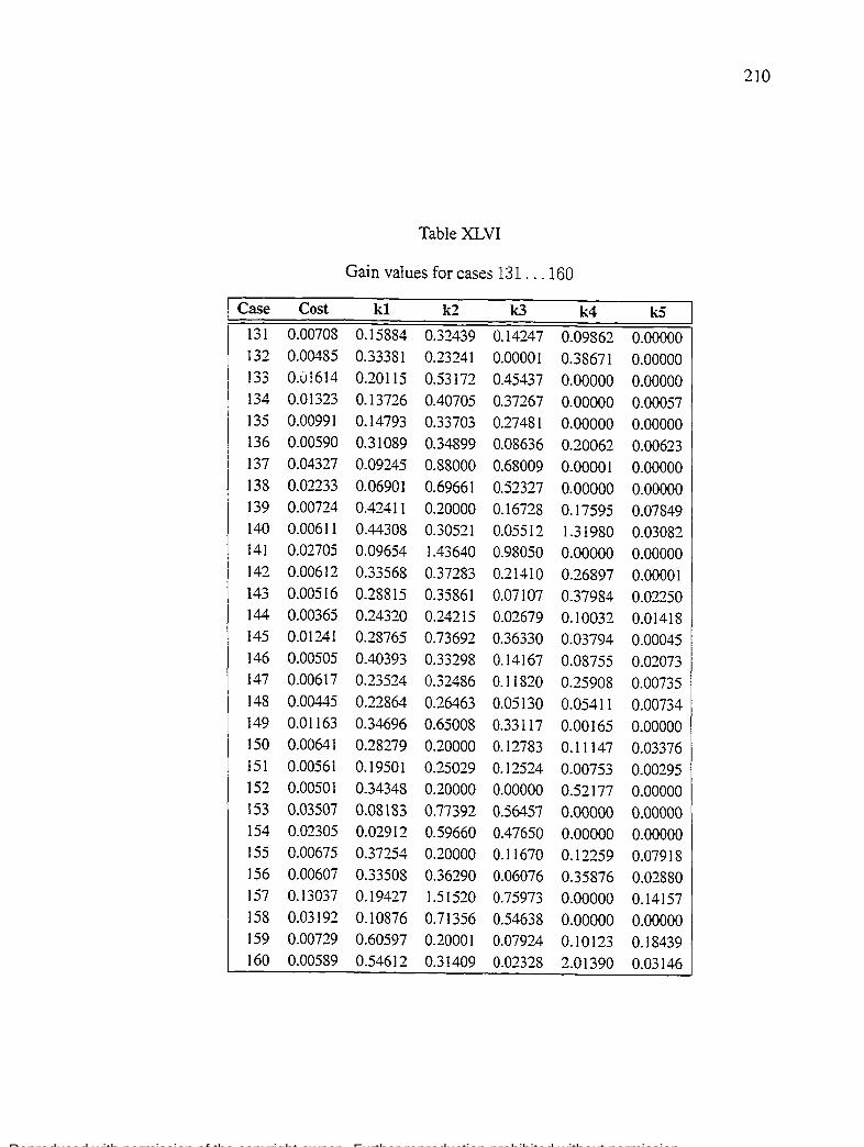
Reproduced with permission of the copyright owner. Further reproduction prohibited without permission.
210
Table XLVI
Gain values for cases 131 ... 160
1 Case Cost kl k2 k3 k4 k5 131 0.00708 0.15884 0.32439 0.14247 0.09862 0.00000 l"'? _,_ 0.00485 0.33381 0.23241 0.00001 0.38671 0.00000 133 O.v!614 0.20115 0.53172 0.45437 0.00000 0.00000 134 0.01323 0.13726 0.40705 0.37267 0.00000 0.00057 135 0.00991 0.14793 0.33703 0.27481 0.00000 0.00000 136 0.00590 0.31089 0.34899 0.08636 0.20062 0.00623 137 0.04327 0.09245 0.88000 0.68009 0.00001 0.00000 138 0.02233 0.06901 0.69661 0.52327 0.00000 0.00000 139 0.00724 0.42411 0.20000 0.16728 0.17595 0.07849 140 0.00611 0.44308 0.30521 0.05512 1.31980 0.03082 141 0.02705 0.09654 1.43640 0.98050 0.00000 0.00000 142 0.00612 0.33568 0.37283 0.21410 0.26897 0.00001 143 0.00516 0.28815 0.35861 0.07107 0.37984 0.02250 144 0.00365 0.24320 0.24215 0.02679 0.10032 0.01418 145 0.01241 0.28765 0.73692 0.36330 0.03794 0.00045 146 0.00505 0.40393 0.33298 0.14167 0.08755 0.02073 147 0.00617 0.23524 0.32486 0.11820 0.25908 0.00735 148 0.00445 0.22864 0.26463 0.05130 0.05411 0.00734 149 0.01163 0.34696 0.65008 0.33117 0.00165 0.00000 150 0.00641 0.28279 0.20000 0.12783 0.11147 0.03376 151 0.00561 0.19501 0.25029 0.12524 0.00753 0.00295 152 0.00501 0.34348 0.20000 0.00000 0.52177 0.00000 153 0.03507 0.08183 0.77392 0.56457 0.00000 0.00000 154 0.02305 0.02912 0.59660 0.47650 0.00000 0.00000 155 0.00675 0.37254 0.20000 0.11670 0.12259 0.07918 156 0.00607 0.33508 0.36290 0.06076 0.35876 0.02880 157 0.13037 0.19427 1.51520 0.75973 0.00000 0.14157 158 0.03192 0.10876 0.71356 0.54638 0.00000 0.00000 159 0.00729 0.60597 0.20001 0.07924 0.10123 0.18439 160 0.00589 0.54612 0.31409 0.02328 2.01390 0.03146

Reproduced with permission of the copyright owner. Further reproduction prohibited without permission.
BIBLIOGRAPHY
Angeline, P. J. (1995). Adaptive and self-adaptive evolutionary computation. In M. Palaniswami, Y. Attikiouzel, R. J. Marks, D. Fogel, and T. Fukuda (Eds.), Computational Intelligence: A Dynamic System Perspective, pp. 1995. IEEE press.
Arabas, J., Z. Michalewicz, and J. Mulawka (1994). Gavaps - a genetic algorithm with varying population size. In Proceedings of The First IEEE Conference on Evolutionary Computation, pp. 73-78.
Aranda, J., J. M. d. 1. Cruz, M. Parrilla, and P. Ruiperez (2000). Evolutionary algorithms for the design of a multivariable control for an aircraft flight control. In AIAA Guidance, Navigation, and Control Conference and Exhibit, Denver, CO. American Institute of Aeronautics and Astronautics, Reston, VA.
Amone, S., M. Dell'Orto, and A. Tettamanzi (1994). Toward a fuzzy government of genetic population. In Proceedings of the 6th IEEE Conference on Tools with Artificial Intelligence, Los Alamitos, CA, pp. 101-111. IEEE Computer Society Press.
Back, T. (1996). Evolutionary Algorithms in TheO!)' and Practice. Oxford University Press.
Back, T. and F. Hoffmeister ( 1991 ). Extended selection mechanisms in gene tic algorithms. In R. K. Belew and L. B. Booker (Eds.), Fourth Intemational Conference on Genetic Algorithms, San Diego, pp. 92-99. University of Califomia: Morgan Kaufmann.
Back, T., F. Hoffmeister, and H. Schwefel (1991 ). A survey of evolution strategies.
Back, T. and M. Schütz ( 1996). Intelligent mutation rate control in canonical genetic algorithms. In Z. Ras and M. Michalewicz (Eds.), Foundations of Intelligent Systems, Number 1079 in Lecture Notes in Artificial Intelligence, pp. 158-167. Springer-Verlag.
Baker, J. E. (1985). Adaptive selection methods for genetic algorithms. In J. J. Grefenstette (Ed.), International Conference on Genetic Algorithms, Camegie-Mellon University, Pittsburgh, PA, pp. 101-111.
Baker, J. E. (1987). Reducing bias and inefficiency in the selection algorithm. In Proceedings of the Second International Conference on Genetic Algorithms on Genetic algorithms and their application, pp. 14-21. Lawrence Erlbaum Associates, Inc.
Barr, R. S., B. L. Golden, J. P. Kelly, M. G. Resende, and W. R. Stewart (1995). Designing and reporting on computational experiments with heuristic methods. Journal of Heuristics 1 (1 ), 9-32.

Reproduced with permission of the copyright owner. Further reproduction prohibited without permission.
212
Bean, J. C. and A. B. Hadj-Alouane (1992). A Dual Genetic Algorithm for Bounded Integer Programs. Technical Report TR 92-53, Department of Industrial and Operations Engineering, The University of Michigan. To appear in R.A.I.R.O.-R.O. (invited submission to special issue on GAs and OR).
Bedau, M., M. Giger, and M. Zwick ( 1995). Diversity dynamics in static res ource models.
Beer, R. D. and J. C. Gallagher (1992). Evolving dynamical neural networks for adaptive behavior. Adaptive Belzavior 1(1). 91-122.
Beyer, H.-G. and K. Deb (2001). On self-adaptive features in real parameter evolutionary algorithms. IEEE Transactions on Evolutionary Computation 5(3), 250-270.
Beyer, H.-G. and H.-P. Schwefel (2002). Evolution strategies: A comprehensive introduction. Natural Computing: an international journal] (1 ), 3-52.
Blickle, T. and L. Thiele (1995). A mathematical analysis of toumament selection. In L. Eshelman (Ed.), Proceedings of the Sixth International Conference on Genetic Algorithms, San Francisco, CA, pp. 9-16. Morgan Kaufmann.
Blickle, T. and L. Thiele (1996). A comparison of selection schemes used in evolutionary algorithms. Evolutionary Computation 4( 4 ), 361-394.
Booker, L. (1987). Improving search in genetic algorithms. In L. Davis (Ed.), Genetic Algorithms and Simulated Annealing, Los Altos, pp. 61-73. Morgan Kaufmann Pub1ishers.
Boukhari, H. (2002, May). Optimisation échelonnement des gains d'un contrôleur d'avion en tangage en utilisatn les algorithmes génétiques. Master thesis, École de Technologie Supérieure, Montrêal, Canada.
Bramlette, M. F. (1991 ). Initialization, mutation and selection methods in genetic algorithms for function optimization. In R. Belew and L. B. Booker (Eds.), Proceedings of the Fourth International Conference on Gene tic Algorithms, San Mateo, pp. 100-107. Morgan Kaufmann Publishers.
Cantu-Paz, E. (2002). Order statistics and selection methods of evolutionary algorithms. Information Processing Letters 82(1), 15-22.
Chen, B.-S. and Y.-M. Cheng (1998). A structure-specified hoo optimal control design for practical applications: A genetic approach. IEEE Transactions on Control Systems Technology 6(6), 707-718.
Coello, C. A. ( 1999). A Survey of Constraint Handling Techniques used with Evolutionary Algorithms. Technical Report Lania-RI-99-04, Laboratorio Nacional de Informatica Avanzada, Xalapa, Veracruz, México. (Disponible en: http://www.lania.mxrccoello/constraint.html).

Reproduced with permission of the copyright owner. Further reproduction prohibited without permission.
213
Coello, C. A. and E. Mezura-Montes (2002, April). Handling Constraints in Genetic Algorithms Using Dominance-Based Toumaments. In I. Parrnee (Ed.), Proceedings of the Fifth Intemational Conference on Adaptive Computing Design and Manufacture (ACDM 2002), Volume 5, University of Exeter, Devon, UK, pp. 273-284. Springer-Verlag.
Crawford, L. S., V. H. L. Cheng, and P. K. Menon (1999). Synthesis of flight vehicle guidance and controllaws using genetic search methods. In AIAA Guidance, Navigation, and Control Conference and Exhibit, Portland, OR. American Institute of Aeronautics and Astronautics, Reston, VA.
Daily, D. S. (2005, 06). The online news publication for paris air show 99.
Davis, L. (1989). Adapting operator probabilities in genetic algorithms. In D. Schaffer (Ed.), Proceedings of the Third Intemational Conference on Genetic Algorithms, San Mateo, pp. 61-69. Morgan Kaufmann Publishers.
De Jong, K. A. and W. M. Spears ( 1990). An analysis of the interacting roles of population size and crossover in genetic algorithms. In International Workshop Parallel Problem Solvingfrom Nature, University of Dortmund, pp. 38-47.
Deb, K. (2000). An Efficient Constraint Handling Method for Genetic Algorithms. Computer Methods in Applied Mechanics and Engineering 186, 311-338.
Deb, K. (2003). A population-based algorithm-generator for real-parameter optimization. Technical2003003, KanGAL, Indian Institute ofTechnology, Kanpur.
Deb, K. and R. B. Agrawal (1995). Simulated binary crossover for continuous search space. Complex Systems 9, 115-148.
Deb, K. and S. Agrawal (1999, April). A niched-penalty approach for constraint handling in genetic algorithms. In Proceedings of ICANNGA-99, Portoroz, Slovenia.
Deb, K. and D. E. Goldberg (1989, Jun). An investigation of niche and species formation in genetic function optimization. In D. Schaffer (Ed.), Proceedings of the Third International Conference on Genetic Algorithms, San Mateo, California, pp. 42-50. Giorge Mason University: Morgan Kaufmann.
Deb, K. and M. Goyal (1996). A combined genetic adaptive search geneas for engineering design. Computer Science and Infonnatics 26(4), 30-45.
DeJong, K. (1975). An Analysis of the Behavior of a Class of Genetic Adaptive Systems. Ph.d. dissertation, University of Michigan.
Eiben, A., R. Hinterding, and Z. Michalewicz (1999). Parameter control in evolutionary algorithms. IEEE Transaction on Evolutionary Computation 3(2), 124-141.

Reproduced with permission of the copyright owner. Further reproduction prohibited without permission.
214
Eshe1man, L. J. and J. D. Schaffer (1992). Rea1-coded genetic algorithms and intervalschemata. In L. D. Whitley (Ed.), Foundations of Genetic Algorithms 2. FOGA2 (1993 ed.)., pp. 187-202. San Mateo, California: Morgan Kaufmann Publishers.
Etkin, B. ( 1959). Dynamics of Flight. New York: John Wi1ey and Sons !ne.
Fiacco, A. V. and G. P. McCormick (1968). Nonlinear Programming: Sequential Unconstrained Minimization Techniques. Wiley, New York.
Fogarty, T. C. (1989). Varying the probability of mutation in the genetic algorithm. In D. Schaffer (Ed.), Proceedings of the Third International Conference on Genetic Algorithms, San Mateo, pp. 104-109. Morgan Kaufmann Publishers.
Fogel, D. B. and J. W. Atmar (1990). Comparing genetic operators with gaussian mutation in simulated evolutionary processes using linear systems. Biological Cybemetics 63, 111-114.
Fonseca, C. M. and P. J. Fleming (1998). Multiobjective optimization and multiple constraint handling with evolutionary algorithms-Part I: A uni fied formulation. IEEE Transactions on Systems, Man, and Cybemetics, Part A: Systems and Humans 28(1), 26-37.
Francis, B. A. (1987). A Course in H00 Control The01·y. Berlin, Germany: SpringerVerlag.
Fukunaga, A. S. (1998). Restart scheduling for genetic algorithms. In Proceedings of Fiftlz International Conference on Parallel Problem Solving from Nature (PPSN-V), pp. 357-366. Springer Verlag.
Garda, S., M. Saad, and O. Akrif (2001). Genetic algorithms for the optimization of gains of a civil aircraft control system. In M. H. Hamza (Ed.), /ASTED International Conference onAriificial Intelligence and Soft Computing, Cancun, Mexico, pp. 221-225. International Association of Science and Technology for Development-IASTED.
Garda, S., M. Saad, and O. Akrif (2003). Gains optimization of a fly-by-wire control control system using a real coded genetic algorithm. In Fourth International Conference on Industrial Automation, Montreal, Canada, pp. AI-08.
Garcfa, S., M. Saad, and O. Akrif (2005). Detecting convergence in genetic algorithms with decreasing mutation policies. In M. H. Hamza (Ed.), IASTED International Conference on COMPUTATIONAL INTELLIGENCE, Calgary, Canada, pp. -. International Association of Science and Technology for Development-IASTED.
Garda, S., M. Saad, and O. Akrif (2006). Nonlinear tuning of aircraft controllers using genetic global optimisation:a new periodic mutation operator. To be published in Canadian Journal of Electrical and Computer Engineering.

Reproduced with permission of the copyright owner. Further reproduction prohibited without permission.
215
Gen, M. and R. Cheng (1997). Genetic algorithms and engineering design. Wiley series in Engineerign Design and Automation. New York: John Wiley and Sons, Inc.
Gen, M. and R. Cheng (2000). Genetic Algorithms and Engineering Optimization (2000 ed.). Engineering Design and Automation. John Wiley and Sons, Inc.
Goldberg, D. (1990). Real-coded genetic algorithms, virtual alphabets, and blocking. Technical Report 90001, University of Illinois at Urbana-Champaign.
Go1dberg, D. and K. Deb (1991). A comparative analysis of selection schemes used in genetic algorithms, pp. 69-93. San Mateo, CA: Morgan Kaufman.
Goldberg, D. E. (1989). Genetic algorithms in search, optimization, and machine learning. Addison-Wesley Publishing Company, Inc.
Gong, D., F. Pan, and X. Sun (2002). Research on a novel adaptive genetic algorithm. In Proceedings of the 2002 IEEE International Symposium on /ndustrial Electronics, 2002. /SIE 2002, Volume 1, pp. 357- 360.
Government (1990). Flying qualities of piloted aircraft. Technical report, Government Printing Office.
Hamida, S. B. and A. Petrowski (2000). The need for improving the exploration operators for constrained optimization problems. In Proc. of the 2000 Congress on Evolutionary Computation, Piscataway, NJ, pp. 1176-1183. IEEE Service Center.
Ham ida, S. B. and M. Schoenauer (2000). An adaptive algorithm for constrained optimization problems. In M. Schoenauer, K. Deb, G. Rudolph, X. Yao, E. Lutton, J. J. Merelo, and H.-P. Schwefel (Eds.), Parallel Problem Solving from Nature - PPSN VI, Berlin, pp. 529-538. Springer.
Harper Jr., R. P. and G. E. Cooper ( 1986). Hnadling qualities and pilot evaluation. Journal of Guidance and Control9(5), 515-529.
Herrera, F., E. Herrera-Viedma, and J. L. Lozano, M. Verdegay (1994). Fuzzy tools to improve genetic algorithms. pp. 1532-1539. Proceedings of the Second European Congress on Intelligent Techniques and Soft Computing.
Herrera, F. and M. Lozano (1996). Adaptation of genetic algorithm parameters based on fuzzy Iogic controllers. In F. Herrera and J. L. Verdegay (Eds.), Genetic Algorihtms and Soft Computing, pp. 95-125. Physica-Verlag.
Herrera, F., M. Lozano, and A. M. Sànchez (2003). A taxonomy for the crossover operator for real-coded genetic algorithms: An experimental study. International Journal of Intelligent Systems 18(3), 309-338.

Reproduced with permission of the copyright owner. Further reproduction prohibited without permission.
216
Herrera, F., M. Lozano, and J. L. Verde gay ( 1998). Tackling real-coded genetic algorithms: Operators and tools for behavioural analysis. Arti.ficial Intelligence Review 12(4), 265-319.
Hesser, J. and R. Mann er (1991 ). Towards an optimal mutation probability for genetic algorithms. In H.-P. Schewefel and R. Manner (Eds.), Proceedings ofthe lst Conference on Parallel Solving from Nature, Number 496 in Lecture Notes in Computer Science, pp. 23-32. Springer-Verlag.
Hinterding, R. and Z. Michalewicz (1998, May). Your Brains and My Beauty: Parent Matching for Constrained Optimisation. In Proceedings of the 5th International Conference on Evolutionary Computation, Anchorage, Alaska, pp. 810-815.
Hinterding, R., Z. Michalewicz, and A. E. Eiben (1997). Adaptation in evolutionary computation: A survey. In Proceedings of the 4th IEEE Conference on Evolutionary Computation, pp. 65-69. IEEE Press.
Hodgkinson, J. (1999). Aircraft Handling Qualities. Reston, Virginia: American Institute of Aeronautics and Astronautics.
Bolland, J. H. (1992). Adaptation in Natural and Artificial Sytems : an introductory Analysis with Applications to Biology, Control, and Artificial Intelligence (ComplexA). Bradford Books.
Homaifar, A., S. H.-Y. Lai, and X. Qi (1994). Constrained optimization via genetic algorithms. Simulation 62, 242-254.
Huang, C.-F. (2002). A Study of Mate Selection in Genetic Algorithms. Ph. D. thesis, Electrical Engineering Department, University of Michigan.
Hulin, M. ( 1997). An optimal stop cri teri on for genetic algorithms: A bayesian approach. In Proc. International Conf on Genetic Algorithms (ICGA), pp. 135-143.
Janikow, C. and Z. Michalewicz (1991). An experimental comparison ofbinary and ftoating point representations in genetic algorithms. In R. K. Belew and L. B. Booker (Eds.), Proceedings of the 4th International Conference on Gene tic Algorithms, pp. 151-157. Morgan Kaufmann.
Joines, J. and C. Houck ( 1994). On the use of non-stationary penalty functions to solve nonlinear constrained optimization problems with gas. In D. Fogel (Ed.), Proceedings of the First IEEE Conference on Evolutionary Computation, Orlando, Florida, pp. 579-584. IEEE Press.
Jong, K. A. D. (1975). An analysis of the belzaviour of a class of genetic adaptive systems. Ph. D. thesis, University of Michigan, Diss. Abstr. Int. 36(10), 5140B, University Microfilms No. 76-9381.

Reproduced with permission of the copyright owner. Further reproduction prohibited without permission.
217
J u1strom, B. A. ( 1995). What have y ou do ne for me late1y? adapting operator probabilities in a steady-state genetic a1gorithm. In L. Eshe1man (Ed.), Proceedings of the Sixth International Conference on Gene tic Algorithms, San Francisco, pp. 81-87. Morgan Kaufmann Publishers.
Juric, M. (1994). Optimizing genetic algorithm parameters for multiple fault diagnosis applications. In Proceedings of the Tenth Conference on Artificial Intelligence for Applications, San Antonio, TX, pp. 434-440.
Kapp1er, C. (1996). Are evo1utionary algorithms improved by large mutations? In H.-M. Voigt, W. Ebeling, l. Rechenberger, and H.-P. Schwefe1 (Eds.), PPSN, Volume 1141 of Lecture Notes in Computer Science, Berlin, Germany, pp. 346-355. Springer.
Kirkpatrick, S. J., C. D. Gelatt, and M. P. Vecchi (1983). Optimization by simulated annea1ing. Science 220, 671-680.
Kita, H. (2001). A comparison study of self-adaptation in evolution strategies and realcoded genetic algorithms. Journal of Evolutionary Computational 9(2), 223-241.
Kita, H. and M. Yamamura ( 1999). A functiona1 specia1ization hypothesis for designing genetic algorithms. In Proceedings of the IEEE International Conference on Systems, Man, and Cybernetics, Volume 1, Piscataway, NJ, pp. 579-584. IEEE: IEEE press.
Kocis, L. and W. Whiten (1997). Computational investigations of 1ow-discrepancy sequences. ACM Trans. Math. Software 23(3), 269-294.
Korb, K. and A. Nicholson (2004). Bayesian Artificial Intelligence. Series in Computer Science and Data Ana1ysis. Boca Raton, Florida, USA: Chapman and Hall!CRC.
Koza, J. R. (1992). Genetic Programming. Cambridge, MA: MIT Press.
Koziel, S. and Z. Michalewicz (1999). Evolutionary Algorithms, Homomorphous Mappings, and Constrained Parameter Optimization. Evolutionary Computation 7( 1 ), 19-44.
Krishnakumar, K. and D. E. Goldberg ( 1992). Control system optimization using genetic algorithms. In Journal of Guidance, Control and Dynamics, Volume 15. American Institute of Aeronautics and Astronautics, Reston, VA.
Krishnakumar, K., R. Swaminathan, S. Garg, and S. Narayanaswamy (1995). Solving large parameter optimization problems using genetic algorithms. In AIAA Guidance, Navigation, and Control Conference and Exhibit, Baltimore, MD. American Institute of Aeronautics and Astronautics, Washington, DC.
Kwakernaak, H. (1985, Oct). Minimax frequency domain performance and robustness optimization of linear feedback systems. IEEE Transactions on Automatic Control 30( 1 0), 994-1004.

Reproduced with permission of the copyright owner. Further reproduction prohibited without permission.
218
Lee, C. C. (1990). Fuzzy logic in control systems: fuzzy logic controller - parts i and ii. IEEE Transactions on Systems, Man, and Cybernetics 20(2), 404-435.
Lee, M. A. and H. Takagi ( 1993). Dynamic control of genetic algorithms using fuzzy logic techniques. In S. Forrest (Ed.), Proc. of the Fifth /nt. Conf on Genetic Algorithms, San Mateo, CA, pp. 76-83. Morgan Kaufmann.
Li, T., C. B. Lucasius, and G. Kateman (1992). Optimization of calibration data with the dynamic genetic algorithm.
Mclean, D. (1990). Automatic Flight Control Systems. Prentice Hall.
Michalewicz, Z. (1995, July). Genetic Algorithms, Numerical Optimization, and Constraints. In L. J. Eshelman (Ed.), Proceedings of the Sixth International Conference on Genetic Algorithms (/CGA-95), San Mateo, Califomia, pp. 151-158. University of Pittsburgh: Morgan Kaufmann Publishers.
Michalewicz, Z. (1996). Genetic Algorithms + Data Structures = Evolution Programs. Artificial Intelligence. Springer-Verlag Berlin Heidelberg.
Michalewicz, Z. and N.F. Attia (1994). Evolutionary Optimization of Constrained Problems. In Proceedings of the 3rd Annual Conference on Evolutional)' Programming, pp. 98-108. World Scientific.
Michalewicz, Z., J. Xiao, and K. Trojanowski (1996). Evolutionary computation: One project, many directions. In International Syposium on Methodologies for Intelligent Systems, pp. 189-201.
Muhlenbein, H. and D. Schlierkamp-Voosen (1993). Predictive models for the breeder genetic algorithm i. Evolutionary Computation 1, 25-50.
Munteanu, C., V. Lazarescu, and C. Radoi ( 1998). A new strategy in optimization using genetic algorithms. ln 9th Mediterranean Electrotechnical Conference, 1998. MELECON 98, Volume 1, pp. 415-419.
Neapolitan, R. E. ( 1990). Probabilistic Reasoning in Expert Systems: Theory and A/gorit/uns. John Wiley and Sons, lnc.
Neapolitan, R. E. (2004). Learning Bayesian Networks. Series in Artificial Intelligence. Prentice Hall.
Pearl, J. (1988). Probabilistic Reasoning in Intelligent Systems: Networks of Plausible Inference. Morgan Kaufmann Publishers, Inc.
Pearl, J. (1995). Handbook of Brain Theory and Neural Networks, Chapter Bayesian networks. Cambridge, Massachusetts: MIT Press.

Reproduced with permission of the copyright owner. Further reproduction prohibited without permission.
219
Pham, D. T. and D. Karaboga (2000). Intelligent Optimisation Techniques: Genetic Algorithms, Tabu Searclz, Simulated Annealing and Neural Networks (2000 ed.). Springer.
Porter, B. (1993). Genetic algorithms in control engineering. In Pacifie International Conference on Aerospace, Science and Technology, Volume 1, pp. 436-442. National Cheng Kung University, Tainan, Taiwan.
Porter, B. and D. Hicks (1994a). Genetic robustification of digital model-following ftightcontrol systems. In Proceedings IEEE National Aerospace and Electronics Conference, Volume 1, pp. 556-563. IEEE.
Porter, B. and D. Hicks (1994b ). Performance measures in the genetic design of digital model-following ftight-control systems. In IEEE National Aerospace and Electronics Conference, Volume 1, pp. 564-570. IEEE.
Porter, B. and D. Hicks (1995a). Generic slow-mode/fast-mode optimization of digital pid controllers. In Proceedings IEEE National Aerospace and Electronics Conference, Volume 1, Dayton, OH, pp. 472-477. IEEE.
Porter, B. and D. Hicks (1995b). Genetic design of unconstrained digital pid controllers. In Proceedings IEEE National Aerospace and Electronics Conference, Volume 1, Dayton, OH, pp. 478-485. IEEE.
Rana, S. (1999, 13-17). The distributional biases of crossover operators. In W. Banzhaf, J. Daida, A. E. Eiben, M. H. Garzon, V. Honavar, M. Jakiela, and R. E. Smith (Eds.), Proceedings of the Genetic and Evolutiona1}· Computation Conference, Volume 1, Orlando, Florida, USA, pp. 549-556. Morgan Kaufmann.
Richardson, J. T., M. R. Palmer, G. Liepins, and M. Hilliard (1989, June). Sorne Guidelines for Genetic Algorithms with Penalty Functions. In J. D. Schaffer (Ed.), Proceedings of the Third International Conference on Genetic Algorithms (ICGA-89), San Mateo, Califomia, pp. 191-197. George Mason University: Morgan Kaufmann Publishers.
Rogers, A. and A. Prügel-Bennett (1997). The dynamics of a genetic algorithm on a model hard optimization problem. Complex Systems 11(6), 437-464.
Runarsson, T. P. and X. Yao (2000, September). Stochastic ranking for constrained evolutionary optimization. IEEE Transactions on Evolutionary Computation 4(3), 284-294.
Schaffer, J. D. and e. al. (1989). A study of control parameters affecting online performance of genetic algorithms for function optimization. In M. Kaufman (Ed.), Proceedings of the Third International Conference on Genetic Algorithms, San Mateo, CA.
Schwefel, H. (1995a). Evolution and Optimum Seeking. New York: Wiley.
Schwefel, H.-P. ( 1981 ). Numberical Optimization of Computer Mode/s. Wiley.

Reproduced with permission of the copyright owner. Further reproduction prohibited without permission.
220
Schwefel, H.-P. (1995b ). Evolution and Optimum Seeking. \Vi ley.
Smith, J. E. and T. C. Fogarty ( 1997, jun). Operator and parameter adaptation in genetic algorith~s. Soft Computing 1 (2), 81-87.
Smith, R. E. (1993). Adaptively resizing populations: an algorithm and analysis. In S. Forrest (Ed.), Proceedings of the Fifth Intemational Conference on Genetic Algorithms, San Mateo, pp. 653-657. Morgan Kaufmann Publishers.
Spears, W. and K. O. Jong (1991). An Analysis of Mufti-Point Crossover, pp. 301-315. San Mateo, CA: Morgan Kaufman.
Srinivas, M. and L. M. Patnaik (1994a). Adaptive probabilities of crossover and mutation in genetic algorithms. IEEE Transaction on Systems, Man, and Cybernetics 24(4), 656-667.
Srinivas, M. and L. M. Patnaik (l994b). Genetic algorithms: A survey. Computers 27(6), 17-26.
Stoorvogel, A. (1992). The H 00 Control Problem: A State-Space Approach. Englewood Cliffs, NJ: Prentice Hall.
Sweriduk, G. D., P. K. Menon, and M. L. Stienberg (1998). Robust command augmentation system design using genetic methods. Technical Report NASA no. 19980223987, AIAA Technical Library.
Syswerda, G. (1989, Morgan Kaufmann). Uniform crossover in genetic algorithms. In J. D. Schaffer (Ed.), Proceedings of the Third International Conference on Genetic Algorithms, pp. 2-9.
Thierens, D. (1997). Selection schemes, elitisit recombination, and selection intensity. In Proceedings of the Seventh International Conference on Genetic Algorithms, pp. 152-159. Morgan Kaufmann.
Thierens, D. (2002). Adaptive mutation rate control schemes in genetic algorithms. In Proceedings of the 2002 IEEE World Congress on Computational Intelligence: Congress on Evolutionary Computation, pp. 980- 985. IEEE Press.
Voigt, H.-M., H. Mühlenbein, and D. Cvetkovic ( 1995). Fuzzy recombination for the breeder genetic algorithm. In L. Eshelman (Ed.), Proceedings of the Sixth International Conference on Genetic Algorithms, San Francisco, CA, pp. 104-111. Morgan Kaufmann.
Whitley, D. (1989). The GENITOR algorithm and selection pressure: Why rank-based allocation of reproductive trials is best. In J. D. Schaffer (Ed.), Proceedings of the Third International Conference on Genetic Algorithms, San Mateo, CA. Morgan Kaufman.

Reproduced with permission of the copyright owner. Further reproduction prohibited without permission.
221
Whitley, D. (2001). An overview of evolutionary algorithms: Practical issues and common pitfalls. Journal of Information and Software Technology ( 43), 817-831.
Wu, A. and I. Garibay (2002). The proportional genetic algorithm: Gene expression in a genetic algorithm.
Xu, H. Y., G. Vukovich, Y. Ichikawa, and Y. Ishii (1994). Fuzzy evolutionary algorihtms and automatic robot trajectory generation. In Proceedings of the First IEEE Conference on Evolutionary Computation, pp. 595-600.
Zhang, B.-T. and J.-J. Kim (2000). Comparison of selection methods for evolutionary optimization. Evolutionary Optimization: An International Journal on the Internet 2(1), 55-70.
Zhu, G., O. Akhrif, L. Saydy, and K. Hentabli (2000). Robustness augmentation of fixed structure ftight control systems viau. In AIAA Guidance, Navigation, and Control Conference and Exhibit, Denver, Colorado. American Institute of Aeronautics and Astronautics.