This article was downloaded by: [69.239.249.174]On: 03 March 2015, At: 15:55Publisher: Taylor & FrancisInforma Ltd Registered in England and Wales Registered Number: 1072954 Registered office: Mortimer House,37-41 Mortimer Street, London W1T 3JH, UK

Click for updates

Journal of Environmental Science and Health, PartA: Toxic/Hazardous Substances and EnvironmentalEngineeringPublication details, including instructions for authors and subscription information:http://www.tandfonline.com/loi/lesa20

Human exposure to unconventional natural gasdevelopment: A public health demonstration ofperiodic high exposure to chemical mixtures inambient airDavid R. Browna, Celia Lewisa & Beth I. Weinbergera

a Southwest Pennsylvania Environmental Health Project, McMurray, Pennsylvania, USAPublished online: 03 Mar 2015.

To cite this article: David R. Brown, Celia Lewis & Beth I. Weinberger (2015) Human exposure to unconventional naturalgas development: A public health demonstration of periodic high exposure to chemical mixtures in ambient air, Journal ofEnvironmental Science and Health, Part A: Toxic/Hazardous Substances and Environmental Engineering, 50:5, 460-472

To link to this article: http://dx.doi.org/10.1080/10934529.2015.992663

PLEASE SCROLL DOWN FOR ARTICLE

Taylor & Francis makes every effort to ensure the accuracy of all the information (the “Content”) containedin the publications on our platform. However, Taylor & Francis, our agents, and our licensors make norepresentations or warranties whatsoever as to the accuracy, completeness, or suitability for any purpose of theContent. Any opinions and views expressed in this publication are the opinions and views of the authors, andare not the views of or endorsed by Taylor & Francis. The accuracy of the Content should not be relied upon andshould be independently verified with primary sources of information. Taylor and Francis shall not be liable forany losses, actions, claims, proceedings, demands, costs, expenses, damages, and other liabilities whatsoeveror howsoever caused arising directly or indirectly in connection with, in relation to or arising out of the use ofthe Content.

This article may be used for research, teaching, and private study purposes. Any substantial or systematicreproduction, redistribution, reselling, loan, sub-licensing, systematic supply, or distribution in anyform to anyone is expressly forbidden. Terms & Conditions of access and use can be found at http://www.tandfonline.com/page/terms-and-conditions

Human exposure to unconventional natural gas development:A public health demonstration of periodic high exposureto chemical mixtures in ambient air

DAVID R. BROWN, CELIA LEWIS and BETH I. WEINBERGER

Southwest Pennsylvania Environmental Health Project, McMurray, Pennsylvania, USA

Directional drilling and hydraulic fracturing of shale gas and oil bring industrial activity into close proximity to residences, schools,daycare centers and places where people spend their time. Multiple gas production sources can be sited near residences. Healthcare providers evaluating patient health need to know the chemicals present, the emissions from different sites and the intensityand frequency of the exposures. This research describes a hypothetical case study designed to provide a basic model thatdemonstrates the direct effect of weather on exposure patterns of particulate matter smaller than 2.5 microns (PM2.5) and volatileorganic chemicals (VOCs). Because emissions from unconventional natural gas development (UNGD) sites are variable, a shortterm exposure profile is proposed that determines 6-hour assessments of emissions estimates, a time scale needed to assistphysicians in the evaluation of individual exposures. The hypothetical case is based on observed conditions in shale gasdevelopment in Washington County, Pennsylvania, and on estimated emissions from facilities during gas development andproduction. An air exposure screening model was applied to determine the ambient concentration of VOCs and PM2.5 atdifferent 6-hour periods of the day and night. Hourly wind speed, wind direction and cloud cover data from PittsburghInternational Airport were used to calculate the expected exposures. Fourteen months of daily observations were modeled. Higherthan yearly average source terms were used to predict health impacts at periods when emissions are high. The frequency andintensity of exposures to PM2.5 and VOCs at a residence surrounded by three UNGD facilities was determined. The findingsshow that peak PM2.5 and VOC exposures occurred 83 times over the course of 14 months of well development. Among thestages of well development, the drilling, flaring and finishing, and gas production stages produced higher intensity exposures thanthe hydraulic fracturing stage. Over one year, compressor station emissions created 118 peak exposure levels and a gas processingplant produced 99 peak exposures over one year. The screening model identified the periods during the day and the specificweather conditions when the highest potential exposures would occur. The periodicity of occurrence of extreme exposures issimilar to the episodic nature of the health complaints reported in Washington County and in the literature. This studydemonstrates the need to determine the aggregate quantitative impact on health when multiple facilities are placed near residences,schools, daycare centers and other locations where people are present. It shows that understanding the influence of air stabilityand wind direction is essential to exposure assessment at the residential level. The model can be applied to other emissions andsimilar sites. Profiles such as this will assist health providers in understanding the frequency and intensity of the human exposureswhen diagnosing and treating patients living near unconventional natural gas development.

Keywords:Diagnostic tools, dispersion air model, exposure patterns, health impacts, unconventional natural gas.

Introduction

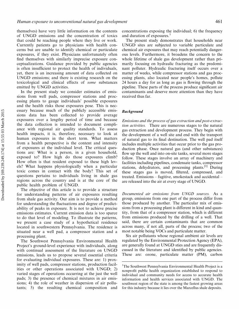
Technological advances in directional drilling and hydrau-lic fracturing have spawned the shale gas boom across theUnited States and around the globe. Progress in the oil

and gas industry has brought industrial activity in closeproximity to residences, schools, day care centers andother places where people spend their time. The short, andeven not-so-short, distances between unconventional natu-ral gas development (UNGD) and everyday human activ-ity allow for emissions from natural gas extraction,processing, and transport to reach individuals in the areaswhere UNGD activities take place.The emissions that occur within several miles of resi-

dences (sometimes less than 500 feet) pose challengesfor health care providers seeing patients from theseareas. Health care providers (as well as patients

Address correspondence to David R. Brown, SouthwestPennsylvania Environmental Health Project, 4198 WashingtonRoad Suite 5, McMurray, PA 15317, USA; E-mail: dbrown@environmentalhealthproject.orgColor versions of one or more of the figures in the article can befound online at www.tandfonline.com/lesa.

Journal of Environmental Science and Health, Part A (2015) 50, 460–472Copyright © 2015 Southwest Pennsylvania Environmental Health ProjectISSN: 1093-4529 (Print); 1532-4117 (Online)DOI: 10.1080/10934529.2015.992663

Dow

nloa

ded

by [

69.2

39.2

49.1

74]

at 1

5:55

03

Mar

ch 2

015

themselves) have very little information on the contentsof UNGD emissions and the concentration of toxicsthat could be reaching people where they live or work.Currently patients go to physicians with health con-cerns but are unable to identify chemical or particulateexposures, if they exist. Physicians unfortunately oftenfind themselves with similarly imprecise exposure con-ceptualizations. Guidance provided by public agenciesis often insufficient to protect the health of individuals,yet, there is an increasing amount of data collected onUNGD emissions; and there is existing research on thetoxicological and clinical effects of some substancesemitted by UNGD activities.In the present study we consider estimates of emis-

sions from well pads, compressor stations and proc-essing plants to gauge individuals’ possible exposuresand the health risks those exposures pose. This is nec-essary because much of the publicly accessible emis-sions data has been collected to provide averageexposures over a lengthy period of time and becausethe data collection is intended to document compli-ance with regional air quality standards. To assesshealth impacts, it is, therefore, necessary to look athuman exposures in the short term. What mattersfrom a health perspective is the content and intensityof exposures at the individual level. The critical ques-tions are: What is a person, in a given household,exposed to? How high do those exposures climb?How often is that resident exposed to these high lev-els? What happens physiologically when a particulartoxic comes in contact with the body? This set ofquestions pertains to individuals living in shale gasregions across the country and is at the core of thepublic health problem of UNGD.The objective of this article is to provide a structure

for understanding patterns of air exposures resultingfrom shale gas activity. Our aim is to provide a methodfor understanding the fluctuations and degree of predict-ability of peaks in exposure. It is not to achieve preciseemissions estimates. Current emission data is too sparceto do that level of modeling. To illustrate the patterns,we present a case study of a hypothetical residencelocated in southwestern Pennsylvania. The residence issituated near a well pad, a compressor station and aprocessing plant.The Southwest Pennsylvania Environmental Health

Project’s ground-level experience with individuals, alongwith continual assessment of the literature on UNGDemissions, leads us to propose several essential criteriafor evaluating individual exposures. These are: 1) prox-imity of well pads, compressor stations, production facil-ities or other operations associated with UNGD; 2)varied stages of operations occurring at the just the wellpads; 3) the presence of chemical mixtures in air emis-sions; 4) the role of weather in dispersion of air pollu-tants; 5) the resulting chemical composition and

concentrations exposing the individual; 6) the frequencyand duration of exposures.1

The present study demonstrates that households nearUNGD sites are subjected to variable particulate andchemical air exposures that may reach potentially danger-ous levels. Furthermore, it broadens the concern to thewhole lifetime of shale gas development rather than pri-marily focusing on hydraulic fracturing as the predomi-nant polluter. Hydraulic fracturing itself occurs over amatter of weeks, while compressor stations and gas proc-essing plants, also located near people’s homes, pollute24 hours a day for as long as gas is flowing through thepipeline. These parts of the process produce significant aircontaminants and deserve more attention than they havereceived thus far.

Background

Emissions and the process of gas extraction and post-extrac-tion activities. There are numerous stages to the naturalgas extraction and development process. They begin withthe development of a well site and end with the transportof natural gas to its final destination. The well pad itselfincludes multiple activities that occur prior to the gas pro-duction phase. Once natural gas (and other substances)flow up the well and into on-site tanks, several more stagesfollow. These stages involve an array of machinery andfacilities including pipelines, condensate tanks, compressorstations, dehydrators, and processing plants.[1] Duringthese stages gas is moved, filtered, compressed, andtreated. Emissions – fugitive, smokestack and accidental –are released into the air at every stage of UNGD.

Documented air emissions from UNGD sources. As agroup, emissions from one part of the process differ fromthose produced by another. The particular mix of emis-sions from a processing plant is different in kind and quan-tity, from that of a compressor station, which is differentfrom emissions produced by the drilling of a well. Thatsaid, there are certain contaminants that are commonacross many, if not all, parts of the process; two of themost notable being VOCs and particulate matter.Six air pollutants whose regional ambient air levels are

regulated by the Environmental Protection Agency (EPA),are generally found at UNGD sties and are frequently dis-cussed in the literature and identified by public agencies.These are: ozone, particulate matter (PM), carbon

1The Southwest Pennsylvania Environmental Health Project is anonprofit public health organization established to respond toindividual and community needs for access to accurate healthinformation and health services associated with UNGD. Thesouthwest region of the state is among the fastest growing areasfor this industry because it lies over the Marcellus shale deposits.

Human exposure to unconventional natural gas development 461

Dow

nloa

ded

by [

69.2

39.2

49.1

74]

at 1

5:55

03

Mar

ch 2

015

monoxide (CO), nitric oxides (NOx), sulfur oxides (SOx),and lead. Also frequently discussed in the emerging litera-ture on UNGD are volatile organic compounds (VOCs)which include aromatic hydrocarbons, halogenated com-pounds, aldehydes, alcohols, and glycols.[2-4] VOCs arereleased into the atmosphere during the production andprocessing of natural gas and as a component of diesel andexhaust.[5] They also are released from gasoline, solvents,paints and other industrial and domestic products.The Pennsylvania Department of Environmental Protec-

tion (PA DEP) inventory of emissions from natural gasfacilities includes CO, NOx, PM10 (particulate matter lessthan 10 microns), PM2.5 (less than 2.5 microns), SOx, theVOCs, Benzene, Ethyl Benzene, Formaldehyde, n-Hexane,Toluene, Xylenes (isomers and mixture), and 2,2,4-Trime-thylpentane.[6] In Washington County, Pennsylvania, thePA Department of Environmental Protection (PA DEP)has collected data on 214 natural gas facilities. The highestlevels of emissions reported were of benzene, PM2.5, NOx,formaldehyde, trimethyl pentene, and ethyl benzene.[7]

Additionally, a study conducted for the City of Fort Worth,Texas found acetaldehyde, butadiene 1,3, carbon disulfide,carbon tetrachloride, and tetrachloroethylene.[8] The TexasCommission on Environmental Quality collects data onNOx, VOCs and HAPs (hazardous air pollutants regulatedbased on emissions rather than regional air levels).[9] Thereare many other known, suspected, and as yet unknown airemissions from UNGD.[1,8,10,11]

Fluctuations in emissions and ambient air dispersal. Wellpad emissions vary in content and concentration overtime. In the lead up to a producing well, different activitiesoccur: drilling, hydraulic fracturing, flowback, flaring and,finishing. In contrast other UNGD facilities operate in amore uniform way over time (such as compressor stationsand processing plants) but still emissions measured nearbyalso vary (see Findings section). In addition to differingreleases of contaminants, emissions disperse from theirsources in varied patterns due to weather and atmosphericconditions. Characterizing these variations– their

intensity, frequency, and duration – is critically importantfrom a public health perspective. Little attention has beenpaid to these fluctuations, particularly the high spikes inexposures.Three short-term air reports from the PA DEP provide a

set of compounds found at well sites, impoundment pondsand compressor stations.[12-14] The PA DEP developed itslist of air contaminants after consulting with the TexasCommission on Environmental Quality, New YorkDepartment of Environmental Conservation, data fromresearch in Dish, TX, the Federal Register, and TERC.[12]

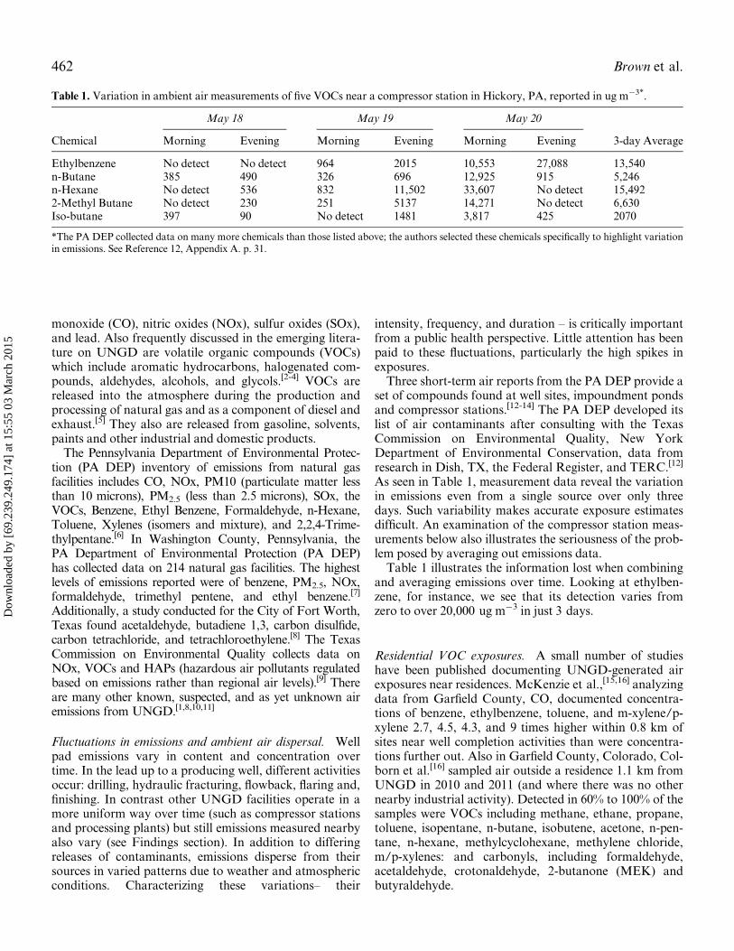
As seen in Table 1, measurement data reveal the variationin emissions even from a single source over only threedays. Such variability makes accurate exposure estimatesdifficult. An examination of the compressor station meas-urements below also illustrates the seriousness of the prob-lem posed by averaging out emissions data.Table 1 illustrates the information lost when combining

and averaging emissions over time. Looking at ethylben-zene, for instance, we see that its detection varies fromzero to over 20,000 ug m¡3 in just 3 days.

Residential VOC exposures. A small number of studieshave been published documenting UNGD-generated airexposures near residences. McKenzie et al.,[15,16] analyzingdata from Garfield County, CO, documented concentra-tions of benzene, ethylbenzene, toluene, and m-xylene/p-xylene 2.7, 4.5, 4.3, and 9 times higher within 0.8 km ofsites near well completion activities than were concentra-tions further out. Also in Garfield County, Colorado, Col-born et al.[16] sampled air outside a residence 1.1 km fromUNGD in 2010 and 2011 (and where there was no othernearby industrial activity). Detected in 60% to 100% of thesamples were VOCs including methane, ethane, propane,toluene, isopentane, n-butane, isobutene, acetone, n-pen-tane, n-hexane, methylcyclohexane, methylene chloride,m/p-xylenes: and carbonyls, including formaldehyde,acetaldehyde, crotonaldehyde, 2-butanone (MEK) andbutyraldehyde.

Table 1. Variation in ambient air measurements of five VOCs near a compressor station in Hickory, PA, reported in ug m¡3*.

May 18 May 19 May 20

Chemical Morning Evening Morning Evening Morning Evening 3-day Average

Ethylbenzene No detect No detect 964 2015 10,553 27,088 13,540n-Butane 385 490 326 696 12,925 915 5,246n-Hexane No detect 536 832 11,502 33,607 No detect 15,4922-Methyl Butane No detect 230 251 5137 14,271 No detect 6,630Iso-butane 397 90 No detect 1481 3,817 425 2070

*The PA DEP collected data on many more chemicals than those listed above; the authors selected these chemicals specifically to highlight variationin emissions. See Reference 12, Appendix A. p. 31.

462 Brown et al.

Dow

nloa

ded

by [

69.2

39.2

49.1

74]

at 1

5:55

03

Mar

ch 2

015

Researchers working with Earthworks sampled air nearresidences in nine counties in Pennsylvania during 2011and 2012. For households between 0.1 km and 8 km fromgas facilities 94% of the samples that were tested for 2-butanone detected it; 88% of those tested for acetone and79% of those tested for chloromethane detected it. Alsofrequently but not as consistently found were 1,1,2-Tri-chloro-1,2,2-trifluoroethane, carbon tetrachloride andtrichlorofluoromethane.[17]

In 2009, Wolf Eagle Environmental, a consulting firmworking for the town of Dish, Texas, sampled air on sevenresidential properties near compressor stations. Chemicalsidentified in the samples drawn included a number thatwere found above Texas’s Effective Screening Levels (lev-els which cause concern for health effects). These includedbenzene, dimethyl disulfide, naphthalene, m & p xylenes,carbonyl sulfide, carbon disulfide, methyl pyridine, anddimethyl pyridine.[11]

Health problems identified in the literature. The onset ofthe acute actions of VOCs and PM2.5 can be very brief,within days, hours or minutes.[18] Many of the studieslisted below find illnesses reported that appear to be shortterm but recurring (Table 2). For instance, burning eyesand throat irritation were found in the research of Bam-berger,[19] Steinzor et al.,[17] and Subra.[20,21] Episodic nau-sea was reported by residents in studies by Ferrar et al.,[22]

Subra,[20] and Bamberger and Oswald.[19] Rabinowitzet al. documents reports of dermatologic and upper respi-ratory symptoms close to well sites.[23]

Rationale. To understand the potential health effects andrisks to residents, it is necessary to conceptualize the inten-sity and patterns of residential exposures to UNGD airemissions. To do this source term estimates needed to bedeveloped and then applied to a pollution dispersionmodel. There is little measurement data providing emis-sion rates for the central UNGD operations: four stages ofwell development at the well pad, compressor stations,and processing facilities. Further, there is great variabilityin emissions over time and among activities and betweensites that is not captured by existing research or by the PADEP. The model provides estimates of exposures at differ-ent distances from UNGD sites. The emissions estimatesused here are provisional; when accurate measurementsand estimates–which reflect the variability–are availablethose could be used.

Materials and methods

Development of the case study. A model is presented for ahypothetical residence in southwest Pennsylvania. The res-idence has one well pad with five wells 1 km to the west, acompressor station 2 km to the south and a processing sta-tion 5 km to the north. This “typical” scenario is based on

a dataset of 276 households in Washington County, Penn-sylvania.[28] 2 It includes two common UNGD facilities –a well pad with multiple wells and a compressor station.We chose to include a processing plant at the furthest dis-tance (5 km) because they are less common yet largeenough to pose potentially significant health risks.

Assumptions. To move forward with a basic screeningmodel, we have made several assumptions:

I. Compressor stations and processing plants are assumedto emit at constant rates and concentrations.II. Each phase of the drill pad development is assumed toemit at a constant rate. That is, the drilling phase isassumed to generate constant emissions, the hydrofrackingphase is assumed to generate constant emissions, etc.III. Terrain is assumed to be flat.IV. Pollutants such as PM2.5 and VOCs are assumed totravel in the same manner.

EHP exposure model. Considering a hypothetical resi-dence with three different sources at 1 km, 2 km and5 km, we model the movement and dilution of emissionsfrom each point source to the residence over a period of14 months. We applied weather conditions reported fromthe Pittsburgh International Airport from February 2011through March 2012. The rates of dilution, based onknown weather effects and distance from the source, arecalculated in 6-h increments. Six-h increments capture thefour time periods that are generally responsive to diurnalweather-based dilution patterns. The 6-h increments aredesignated Night: 12 midnight – 6:00 am; Morning: 6:00am – 12 noon; Afternoon: 12 noon – 6:00 pm; Evening:6:00 pm – 12 midnight. The short time intervals also reflectour interest in capturing the short time periods in whichonset of health reactions can occur.

Calculation of weather/diurnal effects. The exposuremodel is intended to be of use to health care providers andresidents living in shale development areas. It is a basic“box” air pollution dispersion model, based on the seminalwork of Pasquill.[29] Much more complex, accurate air dis-persion models are available to use. Highly accurate dataon UNGD emissions is not yet available and our data isbased on estimates. The simple box model best fits our pur-pose of providing a simple conceptual model that describes

2Two hundred and fourteen of these residences were found tohave between 1 and 77 UNGD well pads at a distance of 2–5km. Eighty-five residences had from 1 to 17 well pads locatedbetween 1–2 km. Thirty-one homes had from 1 to 7 well padswithin 1k km. Two hundred and sixty residences had between 1and 5 compressor stations 2–5 km distant. Fifteen homes had 1–2 compressor stations within 1–2 km. Five residences had one totwo compressor stations less than 1 km distant. WashingtonCounty currently has two processing stations.

Human exposure to unconventional natural gas development 463

Dow

nloa

ded

by [

69.2

39.2

49.1

74]

at 1

5:55

03

Mar

ch 2

015

in general how residents near UNGD are at risk of epi-sodic exposures. See Appendix A for full discussion of thecalculation of effects.The model posits that the emissions at the source are

released into a defined volume of air (the theoretical“box”). We use a “box” 100 meters at the base. The lengthis determined by wind speed (meters per minute) Theheight is dependent on weather and other atmospheric

conditions. The box increases in volume as the air flow car-ries it away from the site, raising the height of dilution andthe width of the plume. A new volume calculation andemission concentration is made at each distance pointreported (in this case, at 1 km, 2 km and 5 km). The largerthe volume of the “box” the more dispersed the pollution.In the model, emissions are assumed to be constant withinevery stage. The terrain is assumed to be flat.Cloud cover, wind speed, wind direction, and portion of

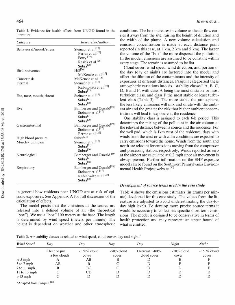
the day (day or night) are factored into the model andaffect the dilution of the contaminants and the intensity ofexposures at different distances. Pasquill categorized theseatmospheric variations into six “stability classes” A, B, C,D, E and F, with class A being the most unstable or mostturbulent class, and class F the most stable or least turbu-lent class (Table 3).[29] The more stable the atmosphere,the less likely emissions will mix and dilute with the ambi-ent air and the greater the risk that higher ambient concen-trations will lead to exposure at the residence.One stability class is assigned to each 6-h period. This

determines the mixing of the pollutant in the air column atthe relevant distance between a source and the residence. Forthe well pad, which is 1km west of the residence, days withwinds from the west or with calm conditions are expected tocarry emissions toward the home. Winds from the south andnorth are relevant for emissions moving from the compressorand processing station, respectively. Winds reported as zeroat the airport are calculated at 0.2 mph since air movement isalways present. Further information on the EHP exposuremodel can be found on the Southwest Pennsylvania Environ-mental Health Project website.[30]

Development of source terms used in the case study

Table 4 shows the emissions estimates (in grams per min-ute) developed for this case study. The values from the lit-erature are adjusted to avoid underestimating the day-to-day high levels. To develop more precise source terms itwould be necessary to collect site specific short term emis-sions. The model is designed to be conservative in terms ofhealth protection and may represent an upper bound ofwhat is emitted.

Table 2. Evidence for health effects from UNGD found in theliterature.

Category Researcher/author

Behavioral/mood/stress Steinzor et al.[17]

Ferrar et al.[22]

Perry [24}

Resick et al.[26]

Subra[20]

Birth outcomes Hill[26]

McKenzie et al.[27]

Cancer risk McKenzie et al.[15]

Dermal Steinzor et al.[17]

Rabinowitz et al.[23]

Subra[33]

Ear, nose, mouth, throat Steinzor et al.[17]

Subra[21]

Subra[20]

Eye Bamberger and Oswald[19]

Steinzor et al.[17]

Subra[21]

Subra[20]

Gastrointestinal Bamberger and Oswald[19]

Steinzor et al.[17]

Ferrar et al.[22]

High blood pressure Subra[21]

Muscle/joint pain Steinzor et al.[17]

Subra[21]

Subra[20]

Neurological Bamberger and Oswald [19]

Subra[21]

Subra[20]

Respiratory Bamberger and Oswald[19]

Steinzor et al.[17]

Rabinowitz et al.[23]

Subra[20]

Table 3. Air stability classes as related to wind speed, cloud cover, day and night.*

Wind Speed Day Day Day Day Night Night

Clear or justa few clouds

< 50% cloudcover

>50% cloudcover

Overcast >80%cloud cover

>50% cloudcover

< 50% cloudcover

< 5 mph A AB B D E F5 to 7 mph AB B C D E F7 to 11 mph B BC C D D E11 to 13 mph C CD D D D D>13 mph C D D D D D

*Adapted from Pasquill.[29]

464 Brown et al.

Dow

nloa

ded

by [

69.2

39.2

49.1

74]

at 1

5:55

03

Mar

ch 2

015

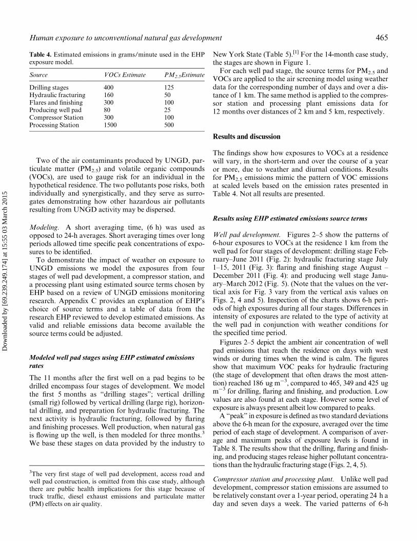
Two of the air contaminants produced by UNGD, par-ticulate matter (PM2.5) and volatile organic compounds(VOCs), are used to gauge risk for an individual in thehypothetical residence. The two pollutants pose risks, bothindividually and synergistically, and they serve as surro-gates demonstrating how other hazardous air pollutantsresulting from UNGD activity may be dispersed.

Modeling. A short averaging time, (6 h) was used asopposed to 24-h averages. Short averaging times over longperiods allowed time specific peak concentrations of expo-sures to be identified.To demonstrate the impact of weather on exposure to

UNGD emissions we model the exposures from fourstages of well pad development, a compressor station, anda processing plant using estimated source terms chosen byEHP based on a review of UNGD emissions monitoringresearch. Appendix C provides an explanation of EHP’schoice of source terms and a table of data from theresearch EHP reviewed to develop estimated emissions. Asvalid and reliable emissions data become available thesource terms could be adjusted.

Modeled well pad stages using EHP estimated emissions

rates

The 11 months after the first well on a pad begins to bedrilled encompass four stages of development. We modelthe first 5 months as “drilling stages”; vertical drilling(small rig) followed by vertical drilling (large rig), horizon-tal drilling, and preparation for hydraulic fracturing. Thenext activity is hydraulic fracturing, followed by flaringand finishing processes. Well production, when natural gasis flowing up the well, is then modeled for three months.3

We base these stages on data provided by the industry to

New York State (Table 5).[1] For the 14-month case study,the stages are shown in Figure 1.For each well pad stage, the source terms for PM2.5 and

VOCs are applied to the air screening model using weatherdata for the corresponding number of days and over a dis-tance of 1 km. The same method is applied to the compres-sor station and processing plant emissions data for12 months over distances of 2 km and 5 km, respectively.

Results and discussion

The findings show how exposures to VOCs at a residencewill vary, in the short-term and over the course of a yearor more, due to weather and diurnal conditions. Resultsfor PM2.5 emissions mimic the pattern of VOC emissionsat scaled levels based on the emission rates presented inTable 4. Not all results are presented.

Results using EHP estimated emissions source terms

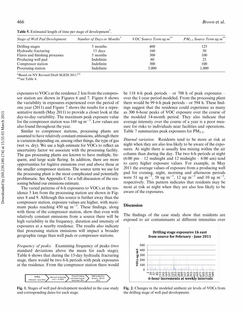
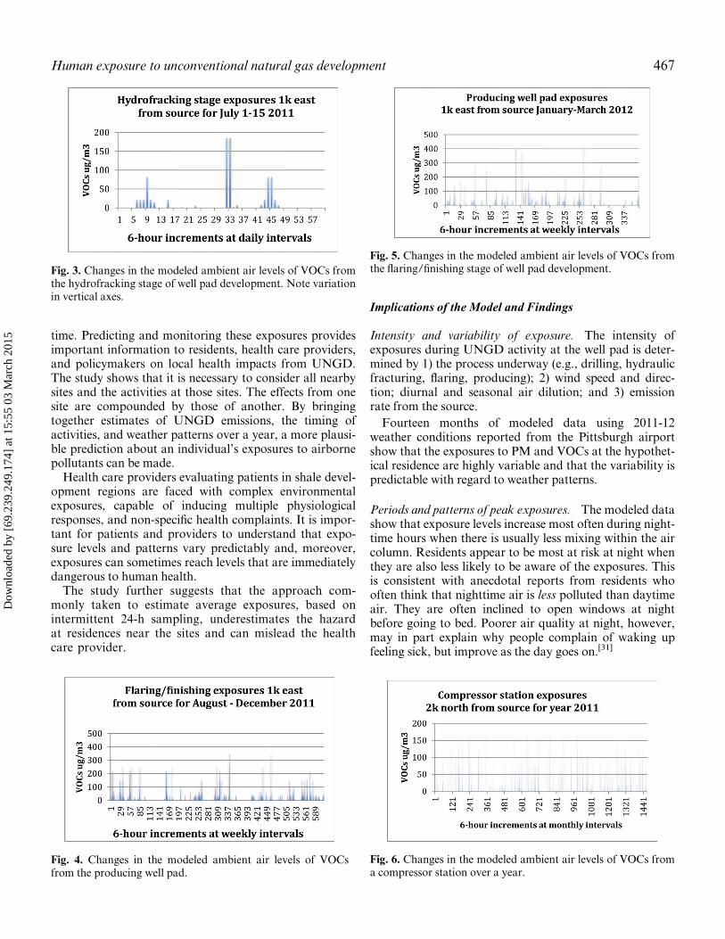
Well pad development. Figures 2–5 show the patterns of6-hour exposures to VOCs at the residence 1 km from thewell pad for four stages of development: drilling stage Feb-ruary–June 2011 (Fig. 2): hydraulic fracturing stage July1–15, 2011 (Fig. 3): flaring and finishing stage August –December 2011 (Fig. 4): and producing well stage Janu-ary–March 2012 (Fig. 5). (Note that the values on the ver-tical axis for Fig. 3 vary from the vertical axis values onFigs. 2, 4 and 5). Inspection of the charts shows 6-h peri-ods of high exposures during all four stages. Differences inintensity of exposures are related to the type of activity atthe well pad in conjunction with weather conditions forthe specified time period.Figures 2–5 depict the ambient air concentration of well

pad emissions that reach the residence on days with westwinds or during times when the wind is calm. The figuresshow that maximum VOC peaks for hydraulic fracturing(the stage of development that often draws the most atten-tion) reached 186 ug m¡3, compared to 465, 349 and 425 ugm¡3 for drilling, flaring and finishing, and production. Lowvalues are also found at each stage. However some level ofexposure is always present albeit low compared to peaks.A “peak” in exposure is defined as two standard deviations

above the 6-h mean for the exposure, averaged over the timeperiod of each stage of development. A comparison of aver-age and maximum peaks of exposure levels is found inTable 8. The results show that the drilling, flaring and finish-ing, and producing stages release higher pollutant concentra-tions than the hydraulic fracturing stage (Figs. 2, 4, 5).

Compressor station and processing plant. Unlike well paddevelopment, compressor station emissions are assumed tobe relatively constant over a 1-year period, operating 24 h aday and seven days a week. The varied patterns of 6-h

Table 4. Estimated emissions in grams/minute used in the EHPexposure model.

Source VOCs Estimate PM2.5Estimate

Drilling stages 400 125Hydraulic fracturing 160 50Flares and finishing 300 100Producing well pad 80 25Compressor Station 300 100Processing Station 1500 500

3The very first stage of well pad development, access road andwell pad construction, is omitted from this case study, althoughthere are public health implications for this stage because oftruck traffic, diesel exhaust emissions and particulate matter(PM) effects on air quality.

Human exposure to unconventional natural gas development 465

Dow

nloa

ded

by [

69.2

39.2

49.1

74]

at 1

5:55

03

Mar

ch 2

015

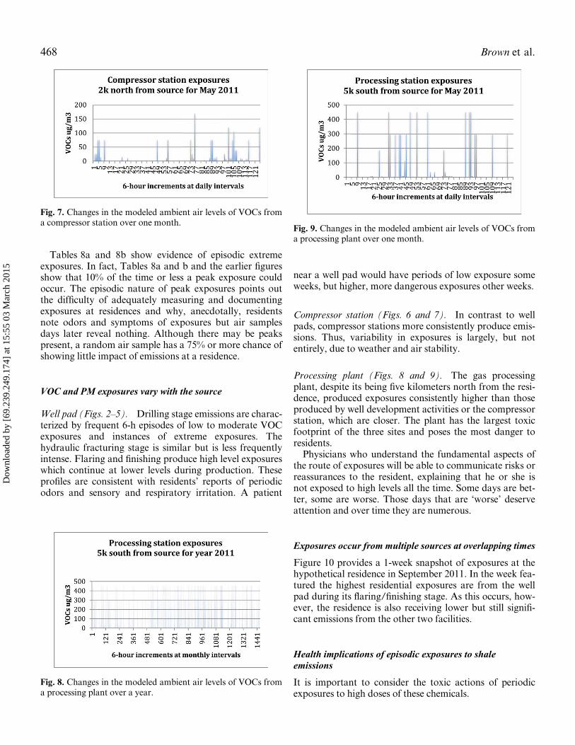
exposures to VOCs at the residence 2 km from the compres-sor station are shown in Figures 6 and 7. Figure 6 showsthe variability in exposures experienced over the period ofone year (2011) and Figure 7 shows the results for a repre-sentative month (May 2011) to provide a closer look at theday-to-day variability. The maximum peak exposure valuefor the compressor station was 169 ug m¡3. Low values arealso found throughout the year.Similar to compressor stations, processing plants are

assumed to have relatively constant emissions, although thereis variation depending on, among other things, the type of gas(wet vs. dry). We use a high estimate for VOCs to reflect anuncertainty factor we associate with the processing facility.The gas processing plants are known to have multiple, fre-quent, and large scale flaring. In addition, there are moreopportunities for fugitive emissions over and above those atthe smaller compressor stations. The source term we use forthe processing plant is the most complicated and potentiallyproblematic. See Appendix C for a full discussion of the rea-soning behind our emissions estimate.The varied patterns of 6-h exposures to VOCs at the res-

idence 5 km from the processing station are shown in Fig-ures 8 and 9. Although this source is further away than thecompressor station, exposure values are higher, with maxi-mum peaks reaching 450 ug m¡3. These findings, alongwith those of the compressor station, show that even withrelatively constant emissions from a source there will behigh variability in the frequency, duration and intensity ofexposures at a nearby residence. The results also indicatethat processing station emissions will impact a broadergeographic range than well pads or compressor stations.

Frequency of peaks. Examining frequency of peaks (twostandard deviations above the mean for each stage),Table 6 shows that during the 15-day hydraulic fracturingstage, there would be two 6-h periods with peak exposuresat the residence. From the compressor station there would

be 118 6-h peak periods – or 708 h of peak exposures –over the 1-year period modeled. From the processing plantthere would be 99 6-h peak periods – or 594 h. These find-ings suggest that the residence could experience as manyas 300 6-hour peaks of VOC exposure over the course ofthe modeled 14-month period. They also indicate thataverage intensity over the course of a year is a poor mea-sure for risks to individuals near facilities and operations.Table 7 summarizes peak exposures for PM2.5.

Diurnal variation. Residents tend to be more at risk atnight when they are also less likely to be aware of the expo-sures. At night there is usually less mixing within the aircolumn than during the day. The two 6-h periods at night(6:00 pm – 12 midnight and 12 midnight – 6:00 am) tendto carry higher exposure values. For example, in May2011 the average values of exposure from a producing wellpad for evening, night, morning and afternoon periodswere 51 ug m¡3, 58 ug m¡3, 12 ug m¡3 and 10 ug m¡3,respectively. This pattern indicates that residents may bemost at risk at night when they are also less likely to beaware of the exposures.

Discussion

The findings of the case study show that residents areexposed to air contaminants at different intensities over

Table 5. Estimated length of time per stage of development*.

Stage of Well Pad Development Number of Days or Months* VOC Source Term ug m** PM2.5 Source Term ug m**

Drilling stages 5 months 400 125Hydraulic fracturing 15 days 160 50Flares and finishing processes 5 months 300 100Producing well pad Indefinite 80 25Compressor station Indefinite 300 100Processing station Indefinite 3,000 1,000

*Based on NY Revised Draft SGEIS 2011.[1]

**see Table 4.

Fig. 1. Stages of well pad development modeled in the case studyand corresponding dates for each stage.

Fig. 2. Changes in the modeled ambient air levels of VOCs fromthe drilling stage of well pad development.

466 Brown et al.

Dow

nloa

ded

by [

69.2

39.2

49.1

74]

at 1

5:55

03

Mar

ch 2

015

time. Predicting and monitoring these exposures providesimportant information to residents, health care providers,and policymakers on local health impacts from UNGD.The study shows that it is necessary to consider all nearbysites and the activities at those sites. The effects from onesite are compounded by those of another. By bringingtogether estimates of UNGD emissions, the timing ofactivities, and weather patterns over a year, a more plausi-ble prediction about an individual’s exposures to airbornepollutants can be made.Health care providers evaluating patients in shale devel-

opment regions are faced with complex environmentalexposures, capable of inducing multiple physiologicalresponses, and non-specific health complaints. It is impor-tant for patients and providers to understand that expo-sure levels and patterns vary predictably and, moreover,exposures can sometimes reach levels that are immediatelydangerous to human health.The study further suggests that the approach com-

monly taken to estimate average exposures, based onintermittent 24-h sampling, underestimates the hazardat residences near the sites and can mislead the healthcare provider.

Implications of the Model and Findings

Intensity and variability of exposure. The intensity ofexposures during UNGD activity at the well pad is deter-mined by 1) the process underway (e.g., drilling, hydraulicfracturing, flaring, producing); 2) wind speed and direc-tion; diurnal and seasonal air dilution; and 3) emissionrate from the source.Fourteen months of modeled data using 2011-12

weather conditions reported from the Pittsburgh airportshow that the exposures to PM and VOCs at the hypothet-ical residence are highly variable and that the variability ispredictable with regard to weather patterns.

Periods and patterns of peak exposures. The modeled datashow that exposure levels increase most often during night-time hours when there is usually less mixing within the aircolumn. Residents appear to be most at risk at night whenthey are also less likely to be aware of the exposures. Thisis consistent with anecdotal reports from residents whooften think that nighttime air is less polluted than daytimeair. They are often inclined to open windows at nightbefore going to bed. Poorer air quality at night, however,may in part explain why people complain of waking upfeeling sick, but improve as the day goes on.[31]

Fig. 3. Changes in the modeled ambient air levels of VOCs fromthe hydrofracking stage of well pad development. Note variationin vertical axes.

Fig. 4. Changes in the modeled ambient air levels of VOCsfrom the producing well pad.

Fig. 5. Changes in the modeled ambient air levels of VOCs fromthe flaring/finishing stage of well pad development.

Fig. 6. Changes in the modeled ambient air levels of VOCs froma compressor station over a year.

Human exposure to unconventional natural gas development 467

Dow

nloa

ded

by [

69.2

39.2

49.1

74]

at 1

5:55

03

Mar

ch 2

015

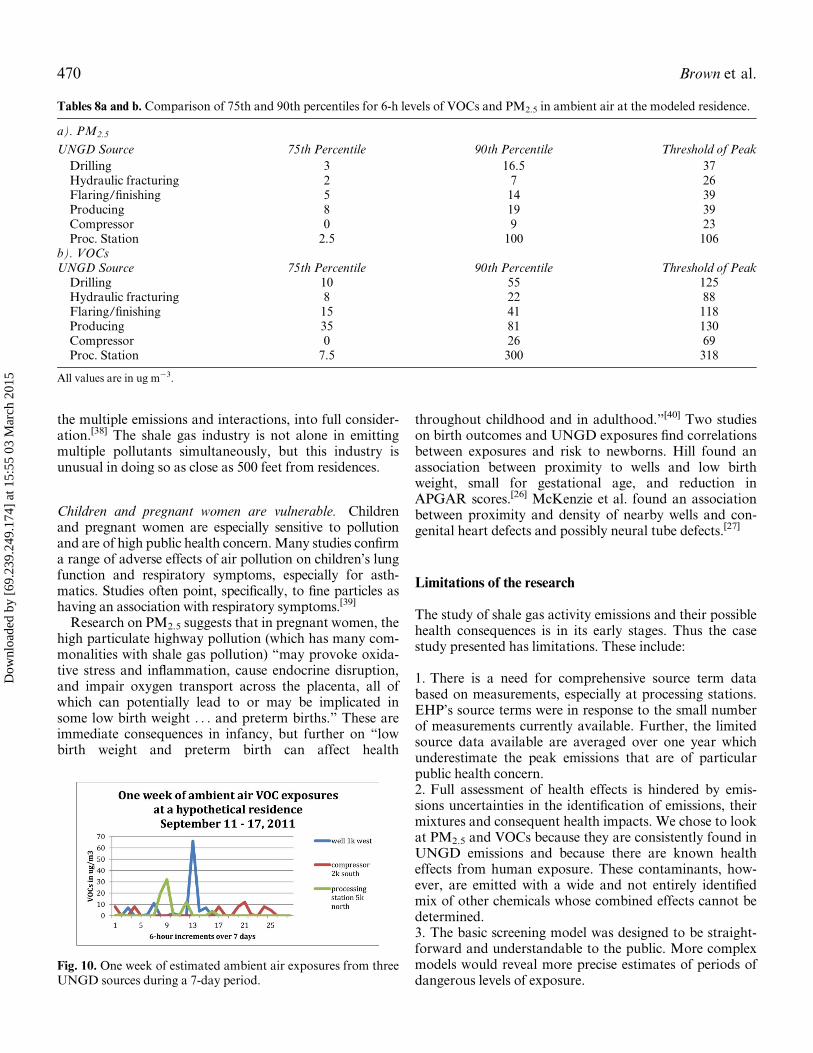
Tables 8a and 8b show evidence of episodic extremeexposures. In fact, Tables 8a and b and the earlier figuresshow that 10% of the time or less a peak exposure couldoccur. The episodic nature of peak exposures points outthe difficulty of adequately measuring and documentingexposures at residences and why, anecdotally, residentsnote odors and symptoms of exposures but air samplesdays later reveal nothing. Although there may be peakspresent, a random air sample has a 75% or more chance ofshowing little impact of emissions at a residence.

VOC and PM exposures vary with the source

Well pad (Figs. 2–5). Drilling stage emissions are charac-terized by frequent 6-h episodes of low to moderate VOCexposures and instances of extreme exposures. Thehydraulic fracturing stage is similar but is less frequentlyintense. Flaring and finishing produce high level exposureswhich continue at lower levels during production. Theseprofiles are consistent with residents’ reports of periodicodors and sensory and respiratory irritation. A patient

near a well pad would have periods of low exposure someweeks, but higher, more dangerous exposures other weeks.

Compressor station (Figs. 6 and 7). In contrast to wellpads, compressor stations more consistently produce emis-sions. Thus, variability in exposures is largely, but notentirely, due to weather and air stability.

Processing plant (Figs. 8 and 9). The gas processingplant, despite its being five kilometers north from the resi-dence, produced exposures consistently higher than thoseproduced by well development activities or the compressorstation, which are closer. The plant has the largest toxicfootprint of the three sites and poses the most danger toresidents.Physicians who understand the fundamental aspects of

the route of exposures will be able to communicate risks orreassurances to the resident, explaining that he or she isnot exposed to high levels all the time. Some days are bet-ter, some are worse. Those days that are ‘worse’ deserveattention and over time they are numerous.

Exposures occur from multiple sources at overlapping times

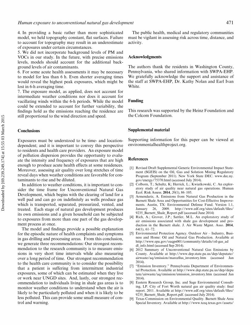
Figure 10 provides a 1-week snapshot of exposures at thehypothetical residence in September 2011. In the week fea-tured the highest residential exposures are from the wellpad during its flaring/finishing stage. As this occurs, how-ever, the residence is also receiving lower but still signifi-cant emissions from the other two facilities.

Health implications of episodic exposures to shale

emissions

It is important to consider the toxic actions of periodicexposures to high doses of these chemicals.

Fig. 7. Changes in the modeled ambient air levels of VOCs froma compressor station over one month.

Fig. 8. Changes in the modeled ambient air levels of VOCs froma processing plant over a year.

Fig. 9. Changes in the modeled ambient air levels of VOCs froma processing plant over one month.

468 Brown et al.

Dow

nloa

ded

by [

69.2

39.2

49.1

74]

at 1

5:55

03

Mar

ch 2

015

Effects from high exposures to VOCs. VOCs are a variedgroup of compounds which can range from having noknown health effects to being highly toxic. Short-termexposure can cause eye and respiratory tract irritation,headaches, dizziness, visual disorders, fatigue, loss ofcoordination, allergic skin reaction, nausea, and mem-ory impairment. Long-term effects include loss of coor-dination and damage to the liver, kidney, and centralnervous system. Some VOCs, such as BTEX (benzene,toluene, ethylbenzene and xylene, which are often emit-ted together), have been detected near natural gas devel-opment and specifically noted by Wolf Eagle, McKenzieet al., Colborn et al., and Steinzor et al.[12,16-18] Acuteexposures to high levels of BTEX have been associatedwith skin and sensory irritation, central nervous systemdepression, and negative effects on the respiratory sys-tem. The case for elevated risk of cancer from UNGDVOC exposure has been made by McKenzie et al.[15]

Effects from high exposure to particulate matter. Expo-sure to PM2.5, in conjunction with other emissions, is ofcore concern. Fine particulates interact with the airborneVOCs increasing their absorption into the lung. Reportedclinical actions resulting from PM2.5 inhalation affect boththe respiratory and cardiovascular systems. Inhalation ofPM2.5 can cause decreased lung function, aggravateasthma symptoms, cause nonfatal heart attacks and highblood pressure.[32] Research reviewing health effects fromhighway traffic, which, like UNGD, has especially highparticulates, concludes, “[s]hort-term exposure to fine

particulate pollution exacerbates existing pulmonary andcardiovascular disease and long-term repeated exposuresincreases the risk of cardiovascular disease and death.”[33]

PM2.5, it has been suggested, “appears to be a risk factorfor cardiovascular disease via mechanisms that likelyinclude pulmonary and systemic inflammation, acceleratedatherosclerosis and altered cardiac autonomic function.Uptake of particles or particle constituents in the bloodcan affect the autonomic control of the heart and circula-tory system.”[33]

High levels of diesel exhaust from engines during well padactivity. Health consequences of diesel exposures includeimmediate and long-term health effects. Diesel emissionscan irritate the eyes, nose, throat and lungs, and can causecoughs, headaches, lightheadedness and nausea. Exposureto diesel exhaust also causes inflammation in the lungs,which may aggravate chronic respiratory symptoms andincrease the frequency or intensity of asthma attacks.Long-term exposure can cause increased risk of lungcancer.[34-37]

Mixtures increase the hazards. Mixtures of pollutants area critically important topic in addressing the public healthimplications of UNGD. While this report has focused sep-arately on two pollutants, in fact, a very large number ofchemicals are released together. Moreover many of thechemicals have little or no tested health data – alone or inconjunction with others. In fact, medical reference valuesdo not take the complex nature of the shale environment,

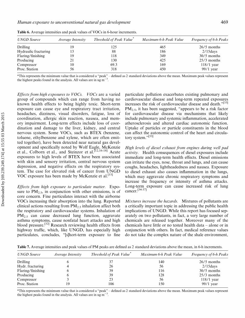
Table 6. Average intensities and peak values of VOCs in 6-hour increments.

UNGD Source Average Intensity Threshold of Peak Value* Maximum 6-h Peak Value Frequency of 6-h Peaks

Drilling 19 125 465 26/5 monthsHydraulic fracturing 13 88 186 2/15daysFlaring/finishing 19 118 349 30/5 monthsProducing 21 130 425 25/3 monthsCompressor 10 69.3 169 118/1 yearProc. Station 56 318 450 99/1 year

*This represents the minimum value that is considered a “peak” – defined as 2 standard deviations above the mean. Maximum peak values representthe highest peaks found in the analysis. All values are in ug m¡3.

Table 7. Average intensities and peak values of PM peaks are defined as 2 standard deviations above the mean, in 6-h increments.

UNGD Source Average Intensity Threshold of Peak Value* Maximum 6-h Peak Value Frequency of 6-h Peaks

Drilling 6 37 140 26/5 monthsHydr. fracturing 4 26 56 2/15daysFlaring/finishing 6 39 116 30/5 monthsProducing 6 39 128 25/3 monthsCompressor 3 23 56 118/1 yearProc. Station 19 106 150 99/1 year

*This represents the minimum value that is considered a “peak” – defined as 2 standard deviations above the mean. Maximum peak values representthe highest peaks found in the analysis. All values are in ug m¡3.

Human exposure to unconventional natural gas development 469

Dow

nloa

ded

by [

69.2

39.2

49.1

74]

at 1

5:55

03

Mar

ch 2

015

the multiple emissions and interactions, into full consider-ation.[38] The shale gas industry is not alone in emittingmultiple pollutants simultaneously, but this industry isunusual in doing so as close as 500 feet from residences.

Children and pregnant women are vulnerable. Childrenand pregnant women are especially sensitive to pollutionand are of high public health concern.Many studies confirma range of adverse effects of air pollution on children’s lungfunction and respiratory symptoms, especially for asth-matics. Studies often point, specifically, to fine particles ashaving an association with respiratory symptoms.[39]

Research on PM2.5 suggests that in pregnant women, thehigh particulate highway pollution (which has many com-monalities with shale gas pollution) “may provoke oxida-tive stress and inflammation, cause endocrine disruption,and impair oxygen transport across the placenta, all ofwhich can potentially lead to or may be implicated insome low birth weight . . . and preterm births.” These areimmediate consequences in infancy, but further on “lowbirth weight and preterm birth can affect health

throughout childhood and in adulthood.”[40] Two studieson birth outcomes and UNGD exposures find correlationsbetween exposures and risk to newborns. Hill found anassociation between proximity to wells and low birthweight, small for gestational age, and reduction inAPGAR scores.[26] McKenzie et al. found an associationbetween proximity and density of nearby wells and con-genital heart defects and possibly neural tube defects.[27]

Limitations of the research

The study of shale gas activity emissions and their possiblehealth consequences is in its early stages. Thus the casestudy presented has limitations. These include:

1. There is a need for comprehensive source term databased on measurements, especially at processing stations.EHP’s source terms were in response to the small numberof measurements currently available. Further, the limitedsource data available are averaged over one year whichunderestimate the peak emissions that are of particularpublic health concern.2. Full assessment of health effects is hindered by emis-sions uncertainties in the identification of emissions, theirmixtures and consequent health impacts. We chose to lookat PM2.5 and VOCs because they are consistently found inUNGD emissions and because there are known healtheffects from human exposure. These contaminants, how-ever, are emitted with a wide and not entirely identifiedmix of other chemicals whose combined effects cannot bedetermined.3. The basic screening model was designed to be straight-forward and understandable to the public. More complexmodels would reveal more precise estimates of periods ofdangerous levels of exposure.

Tables 8a and b. Comparison of 75th and 90th percentiles for 6-h levels of VOCs and PM2.5 in ambient air at the modeled residence.

a). PM2.5

UNGD Source 75th Percentile 90th Percentile Threshold of PeakDrilling 3 16.5 37Hydraulic fracturing 2 7 26Flaring/finishing 5 14 39Producing 8 19 39Compressor 0 9 23Proc. Station 2.5 100 106

b). VOCsUNGD Source 75th Percentile 90th Percentile Threshold of Peak

Drilling 10 55 125Hydraulic fracturing 8 22 88Flaring/finishing 15 41 118Producing 35 81 130Compressor 0 26 69Proc. Station 7.5 300 318

All values are in ug m¡3.

Fig. 10. One week of estimated ambient air exposures from threeUNGD sources during a 7-day period.

470 Brown et al.

Dow

nloa

ded

by [

69.2

39.2

49.1

74]

at 1

5:55

03

Mar

ch 2

015

4. In providing a basic rather than more sophisticatedmodel, we held topography constant, flat surfaces. Failureto account for topography may result in an underestimateof exposures under certain circumstances.5. We did not incorporate background levels of PM andVOCs in our study. In the future, with precise emissionslevels, models should account for the additional back-ground levels of air contaminants.6. For some acute health assessments it may be necessaryto model for less than 6 h. Even shorter averaging timeswould reveal the highest peak exposures, which might belost in 6-h averaging time.7. The exposure model, as applied, does not account forintermediate weather conditions nor does it account forvacillating winds within the 6-h periods. While the modelcould be extended to account for further variability, thefindings hold as the emissions reaching the residence arestill proportional to the wind direction and speed.

Conclusions

Exposures must be understood to be time- and location-dependent; and it is important to convey this perspectiveto residents and health care providers. An exposure modelof pollution dispersion provides the opportunity to evalu-ate the intensity and frequency of exposures that are highenough to produce acute health effects at some residences.Moreover, assessing air quality over long stretches of timereveal days when weather conditions are favorable for con-taminants to rise and be diluted.In addition to weather conditions, it is important to con-

sider the time frame for Unconventional Natural GasDevelopment, which begins with the clearing of land for awell pad and can go on indefinitely as wells produce gaswhich is transported, separated, pressurized, vented, andtreated. Each stage of natural gas development producesits own emissions and a given household can be subjectedto exposures from more than one part of the gas develop-ment process at once.The model and findings provide a possible explanation

for the episodic nature of health complaints and symptomsin gas drilling and processing areas. From this conclusion,we generate three recommendations: Our strongest recom-mendation to the research community is to measure emis-sions in very short time intervals while also measuringover a long period of time. Our strongest recommendationto the health care community is to consider the possibilitythat a patient is suffering from intermittent industrialexposures, some of which can be estimated when they liveor work near UNGD sites. And, lastly, our strongest rec-ommendation to individuals living in shale gas areas is tomonitor weather conditions to understand when the air islikely to be particularly polluted and when it is likely to beless polluted. This can provide some small measure of con-trol and warning.

The public health, medical and regulatory communitiesmust be vigilant in assessing risk across time, distance, andactivity.

Acknowledgments

The authors thank the residents in Washington County,Pennsylvania, who shared information with SWPA-EHP.We gratefully acknowledge the support and assistance ofthe staff at SWPA-EHP, Dr. Kathy Nolan and Earl IvanWhite.

Funding

This research was supported by the Heinz Foundation andthe Colcom Foundation.

Supplemental material

Supporting information for this paper can be viewed atenvironmentalhealthproject.org.

References

[1] Revised Draft Supplemental Generic Environmental Impact State-ment (SGEIS) on the Oil, Gas and Solution Mining RegulatoryProgram (September 2011). New York State DEC. www.dec.ny.gov/energy/75370.html (accessed July 2014).

[2] Colborn, T.; Schultz, K; Herrick, L.; Kwiatkowski, C. An explor-atory study of air quality near natural gas operations. HumanEcol. Risk Assess. 2014, 20(1), 86–105.

[3] Armendariz, A. Emissions from Natural Gas Production in theBarnett Shale Area and Opportunities for Cost-Effective Improve-ments. Austin, TX: Environmental Defense Fund. Version 1.1,January 26, 2009. http://www.edf.org/sites/default/files/9235_Barnett_Shale_Report.pdf (accessed June 2014)

[4] Rich, A.; Grover, J.P.; Sattler, M.L. An exploratory study ofair emissions associated with shale gas development and pro-duction in the Barnett shale. J. Air Waste Mgmt. Asso. 2014,64(1), 61–72.

[5] Environmental Protection Agency. Outdoor Air – Industry, Busi-ness and Home: Oil and Natural Gas Production. Available athttp://www.epa.gov/oaqps001/community/details/oil-gas_addl_info.html (accessed Sep 2014).

[6] 2012 Summary of Unconventional Natural Gas Emissions byCounty. Available at http://www.dep.state.pa.us/dep/deputate/airwaste/aq/emission/marcellus_inventory.htm (accessed Jan2014).

[7] “Emission Inventory.” Pennsylvania Department of Environmen-tal Protection. Available at http://www.dep.state.pa.us/dep/deputate/airwaste/aq/emission/emission_inventory.htm (accessed Jan2014).

[8] Eastern Research Group, Inc. and Sage Environmental Consult-ing, LP. City of Fort Worth natural gas air quality study: finalreport. 2011. Available at http://www.edf.org/sites/default/files/9235_Barnett_Shale_Report.pdf. (accessed July 2014).

[9] Texas Commission on Environmental Quality. Barnett Shale AreaSpecial Inventory. Available at http://www.tceq.texas.gov/assets/

Human exposure to unconventional natural gas development 471

Dow

nloa

ded

by [

69.2

39.2

49.1

74]

at 1

5:55

03

Mar

ch 2

015

public/implementation/air/ie/pseiforms/Barnett%20Shale%20Area%20Special%20Inventory.pdf (accessed May 2014).

[10] Ethridge, S.; Shannon Ethridge to Mark R. Vickery. Texas Com-mission on Environmental Quality. Interoffice Memorandum.Available at http://www.tceq.state.tx.us/assets/public/implementation/barnett_shale/2010.01.27-healthEffects-BarnettShale.pdf(accessed June 2014).

[11] Wolf Eagle Environmental Engineers and Consultants. Town ofDISH, Texas ambient air monitoring analysis final report. Septem-ber 15, 2009. Available at http://townofdish.com/objects/DISH_-_final_report_revised.pdf (accessed July 2014).

[12] Southwestern Pennsylvania Marcellus Shale Short-Term AmbientAir Sampling Report. Pennsylvania Department of EnvironmentalProtection. November, 2010.

[13] Northcentral Pennsylvania Marcellus Shale Short-Term AmbientAir Sampling Report. Pennsylvania Department of EnvironmentalProtection. May, 2011.

[14] Northeastern Pennsylvania Marcellus Shale Short-Term AmbientAir Sampling Report. Pennsylvania Department of EnvironmentalProtection, January 2011.

[15] McKenzie, L.M.; Witter, R.Z.; Newman, L.S.; Adgate, J.L.Human health risk assessment of air emissions from developmentof unconventional natural gas resources. Science of the Total Envi-ronment 2012, 424, 9–87.

[16] Colborn, T.; Schultz, K.; Herrick, L.; Kwiatkowski, C. An explor-atory study of air quality near natural gas operations. HumanEcol. Risk Assess. 2014, 20(1), 86–105.

[17] Steinzor, N.; Subra, W.; Sumi, L. Investigating links betweenshale gas development and health impacts through a commu-nity survey project in Pennsylvania. New Solutions 2013,23(1):55–84.

[18] Darrow, L.A.; Klein, M.; Sarnat, J.A.; Mulholland, J.A; Strick-land, M.J.; Sarnat, S.E.; Russell, A.G.; Tolbert, P.E. The use ofalternative pollutant metrics in time-series studies of ambient airpollution and respiratory emergency department visits. J. Expos.Sci. Environ. Epidemiol. 2011, 21(1), 10–19.

[19] Bamberger, M.; Oswald, R.E. Impacts of gas drilling on humanand animal health. New Sols. 2012, 22, 51–77.

[20] Subra, W. Results of health survey of current and former DISH/Clark, Texas residents. December. Earthworks’ Oil and GasAccountability Project, 2009. Available at http://www.earthworksaction.org/files/publications/DishTXHealthSurvey_FINAL_hi.pdf (accessed July 2014).

[21] Subra, W. Community health survey results: Pavilion, WY resi-dents. 2010. http://www.earthworksaction.org/files/publications/PavillionFINALhealthSurvey-201008.pdf (accessed July 2014).

[22] Ferrar, K.J.; Kriesky, J.; Christen, C.J.; Marshall, L.P.; Malone, S.L.; Sharma, R.K.; Michanowicz, D.R.; Goldstein, B.D. Assess-ment and longitudinal analysis of health impacts and stressors per-ceived to result from unconventional shale gas development in theMarcellus Shale region. Inter. J. Occup. Environ. Health 2013,19(2), 104–112.

[23] Rabinowitz, P.M.; Skizovskiy, I.B.; Lamers, V.; Trufan, S.J.; Hol-ford T.R.; Dziura, J.D.; Peduzzi, P.N.; Kane, M.J.; Reif, J.S.;Weiss, T.R.; Stowe, M.H. Proximity to natural gas wells andreported health status: Results of a household survey in Washing-ton County, Pennsylvania. Environmental Health Perspectives

2014; Available at http://ehp.niehs.nih.gov/wp-content/uploads/advpub/2014/9/ehp.1307732.pdf (accessed Sep 2014)

[24] Perry, S. Using ethnography to monitor the community health impli-cations of onshore unconventional oil and gas developments: examplesfromPennsylvania’sMarcellus Shale New Sols. 2013, 23(1), 33–54.

[25] Resick, L.; Knestrick, J.M.; Counts, M.M.; Pizzuto, L.K. Themeaning of health among mid-Appalachian women within the con-text of the environment. J. Environ. Stud. Sci. 2013, 3, 290–296.

[26] Hill, E. Working paper. Unconventional gas development andinfant health: evidence from Pennsylvania. The Charles H. DysonSchool of Applied Economics and Management, Cornell Univer-sity: Ithaca, NY, July 2012.

[27] McKenzie LM, Guo R, Witter R, Savitz DA, Newman LS, Ade-gate JL. Birth outcomes and maternal residential proximity to nat-ural gas development in rural colorado. Environ. Health Perspect.2014, 122(4), 412–417.

[28] Greiner, L.; Resick, L.; Brown, D.; Glaser, D. Self-reported health,function and sense of control in a convenience sample of adult resi-dents of communities experiencing rapid growth of unconventionalnatural gas extraction: A cross-sectional study. Unpublishedreport, Fairfiled University, Fairfield, CT.

[29] Pasquill, F. Atmospheric Diffusion: The Dispersion of WindborneMaterial from Industrial and other Sources; D. Van NostrandCompany, Ltd.: London, 1962.

[30] Southwest Pennsylvania Environmental Health Project “How’s theWeather?” Air Screening Model. 2013. Available at www.environmentalhealthproject.org/health/air/ (accessed July 2014).

[31] Unpublished personal communications between Southwest Penn-sylvania Environmental Health Project staff and residents in Wash-ington County, PA, 2013–2014.

[32] US EPA “Particulate Matter: Health” Available at http://www.epa.gov/pm/health.html (accessed July 2014).

[33] Brugge, D.; Durant, J.L.; Rioux, C. Near-highway pollutants inmotor vehicle exhaust: A review of epidemiologic evidence of car-diac and pulmonary health risks. Environ. Health 2007, 6, 23.

[34] California Office of Environmental Health Hazard Assessment andAmerican Lung Association “Health Effects of Diesel Exhaust”.Available at Oehha.ca.gov/public_info/facts/dieselfacts (accessedJuly 2014).

[35] Zhang, J.J.; McCreanor, J.E.; Cullinan, P.; Chung, K.F.; Ohman-Strickland, P.; Han, I.K.; J€arup, L.; Nieuwenhuijsen, M.J. Healtheffects of real-world exposure to diesel exhaust in persons withasthma. Research Report. Health Effects Institute 2009; 138, 5–109.

[36] McClellan, R.O. Health effects of exposure to diesel exhaust par-ticles. Ann. Rev. Pharmacol. Toxicol. 1987, 27(1), 279–300.

[37] Ris, C. US EPA health assessment for diesel engine exhaust: areview. Inhal Toxicol 2007, 19(S1), 229–239.

[38] Brown, D.; Weinberger, B.; Lewis, C.; Bonaparte, H.; Understand-ing exposure from natural gas drilling puts current air standards tothe test.Rev Environ Health. 2014, 29(4), 277–92.

[39] Li, S.; Williams, G.; Jalaludin, B.; Baker, P. Panel studies of airpollution on children’s lung function and respiratory symptoms: aliterature review. J. Asthma 2012, 49(9), 895–910.

[40] Barrett, J.R. Apples to apples: comparing PM2.5 Exposuresand birth outcomes in understudied countries. Environ. HealthPerspect. 2014, 122, 4. Available at http://ehp.niehs.nih.gov/122-a110/ (accessed Sep 2014).

472 Brown et al.

Dow

nloa

ded

by [

69.2

39.2

49.1

74]

at 1

5:55

03

Mar

ch 2

015