Embed Size (px)
Citation preview
LUND UNIVERSITY
MASTER THESIS
Developing a technique for combining lightand ultrasound for deep tissue imaging
Author:Meng Li
Supervisor:Stefan Kröll
A thesis submitted in fulfillment of the requirementsfor the degree of Master in Photonics
Project duration: Sep. 2017- May 2018
LRAP-546
Department of PhysicsAtomic Physics Division

i
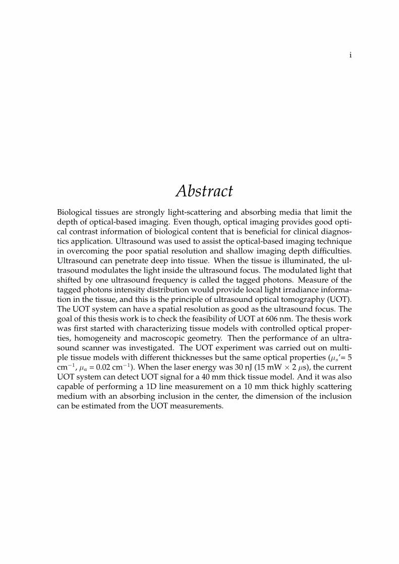
AbstractBiological tissues are strongly light-scattering and absorbing media that limit thedepth of optical-based imaging. Even though, optical imaging provides good opti-cal contrast information of biological content that is beneficial for clinical diagnos-tics application. Ultrasound was used to assist the optical-based imaging techniquein overcoming the poor spatial resolution and shallow imaging depth difficulties.Ultrasound can penetrate deep into tissue. When the tissue is illuminated, the ul-trasound modulates the light inside the ultrasound focus. The modulated light thatshifted by one ultrasound frequency is called the tagged photons. Measure of thetagged photons intensity distribution would provide local light irradiance informa-tion in the tissue, and this is the principle of ultrasound optical tomography (UOT).The UOT system can have a spatial resolution as good as the ultrasound focus. Thegoal of this thesis work is to check the feasibility of UOT at 606 nm. The thesis workwas first started with characterizing tissue models with controlled optical proper-ties, homogeneity and macroscopic geometry. Then the performance of an ultra-sound scanner was investigated. The UOT experiment was carried out on multi-ple tissue models with different thicknesses but the same optical properties (µs’= 5cm−1, µa = 0.02 cm−1). When the laser energy was 30 nJ (15 mW × 2 µs), the currentUOT system can detect UOT signal for a 40 mm thick tissue model. And it was alsocapable of performing a 1D line measurement on a 10 mm thick highly scatteringmedium with an absorbing inclusion in the center, the dimension of the inclusioncan be estimated from the UOT measurements.


iii
AcknowledgementsThere are so many of you I own my thanks for supporting me through my masterthesis work! I would like to express my grandest gratitude to my supervisor StefanKröll. Thank you very much for offering me this fascinating project and spendingcountless hours discussing the project with me, thank you very much for all the ef-forts you put into supervising me. You are so knowledgeable and kind, thank youvery much for always being so concerned and supportive.
I would like to thank Nina Reistad genuinely, thank you very much for sharingyour knowledge in medical optics and allowing me using your experimental setup.The UOT experiment cannot be carried out without your help and support. Andthank you so much for showing me the ongoing photoacoustic tomography (PAT)measurement in Skånes universitetssjukhus, it was so cool to be able to see the PATimaging in clinic application in person. I would like to thank Tobias Erlöv and Mag-nus Cinthio for not only lending me the fancy ultrasound scanner but also spendinga lot of hours sharing me the knowledge of ultrasound. Thank you for always beingthere when I ran into troubles with the scanner.
I would like to thank my friend and colleague Mengqiao Di, thank you very muchfor your company for the last two years during the lectures, lunch, and lab. Andthank you very much for making such an amazing spectral filter to assist the UOTmeasurement, without your hard work I would not be able to complete the project. Iwould like to thank my another friend and colleague Alexander Bengtsson, I appre-ciate all the time you spent in the lab and your assist, and thanks for your cookiestoo.
I would like to thank all my ’co-supervisors’ from the Quantum Information Group,you all are so kind and supportive, thank you for making me always feel welcomed.I would like to specific thanks Chunyan Shi, Sebastian Horvath, Adam Kinos andQian Li. Thank you all so much for using your ’magic power’ bring the 606 nm laserfrom ’dying’ to ’alive’, thank you very much for spending your free time to help me.And thanks Sebastian again for ’resurrected’ my photomultiplier tube as well, thatliterately saved my project. Thank you very much David Hill for proofing readingmy thesis and your comments, they are of great help.
I would like to thank my friends for always being there for me. Especially thanksVidar Flodgren for proofreading my popular science. Now it is yours and Tim’s turnto choose your adventure book, good luck!
Personally, I would like to thank my family my love Karl Bastos. You are always sopatient and so kind. Thank you for your full-time support and care and love.

v
Popular ScienceThe discovery of X-rays was the key to developing medical imaging methods. Sincethen, medical imaging techniques have advanced to the point where it can providereal-time, 2D or 3D, visual representations of the internal structures of a humanbody. The three most commonly used techniques are MRI, CT, and PET scans, allwith their advantages and disadvantages. The MRI uses a strong magnetic fieldto reconstruct an image from resonating atoms, but this means that patients withmetal implants, like pacemakers, cannot perform an MRI scan. Patients can also beallergic to the radiotracers used in the PET scan, and exposure to the X-rays duringa CT-scan carries a risk of cancer. Thus, the world is still looking for other imagingtechniques that can overcome those limitations.
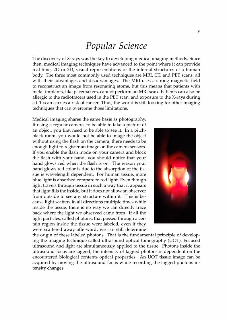
Medical imaging shares the same basis as photography.If using a regular camera, to be able to take a picture ofan object, you first need to be able to see it. In a pitch-black room, you would not be able to image the objectwithout using the flash on the camera, there needs to beenough light to register an image on the camera sensors.If you enable the flash mode on your camera and blockthe flash with your hand, you should notice that yourhand glows red when the flash is on. The reason yourhand glows red color is due to the absorption of the tis-sue is wavelength dependent. For human tissue, moreblue light is absorbed compare to red light. Even thoughlight travels through tissue in such a way that it appearsthat light fills the inside, but it does not allow an observerfrom outside to see any structure within it. This is be-cause light scatters in all directions multiple times whileinside the tissue, there is no way we can directly traceback where the light we observed came from. If all thelight particles, called photons, that passed through a cer-tain region inside the tissue were labeled, even if theywere scattered away afterward, we can still determinethe origin of these labeled photons. That is the fundamental principle of develop-ing the imaging technique called ultrasound optical tomography (UOT). Focusedultrasound and light are simultaneously applied to the tissue. Photons inside theultrasound focus are tagged; the intensity of tagged photons is dependent on theencountered biological contents optical properties. An UOT tissue image can beacquired by moving the ultrasound focus while recording the tagged photons in-tensity changes.

vii
Contents
Abstract i
Acknowledgements iii
Popular Science v
1 Introduction 11.1 Motivation . . . . . . . . . . . . . . . . . . . . . . . . . . . . . . . . . . 11.2 Aim . . . . . . . . . . . . . . . . . . . . . . . . . . . . . . . . . . . . . 2
2 Theoretical Background 32.1 Light-tissue interactions, scattering and absorption . . . . . . . . . . 3
2.1.1 Scattering coefficient . . . . . . . . . . . . . . . . . . . . . . . . 42.1.2 Absorption coefficient . . . . . . . . . . . . . . . . . . . . . . . 6
2.2 Light propagation within the tissue . . . . . . . . . . . . . . . . . . . . 72.2.1 Monte Carlo simulation . . . . . . . . . . . . . . . . . . . . . . 82.2.2 Photon time of flight spectroscopy . . . . . . . . . . . . . . . . 9
2.3 Ultrasound optical tomography . . . . . . . . . . . . . . . . . . . . . . 102.3.1 Ultrasound and focus . . . . . . . . . . . . . . . . . . . . . . . 112.3.2 Acousto-optics . . . . . . . . . . . . . . . . . . . . . . . . . . . 132.3.3 Acousto-optic imaging . . . . . . . . . . . . . . . . . . . . . . . 142.3.4 Basic principle of spectral hole burning . . . . . . . . . . . . . 14
3 Experiment 163.1 Tissue-mimicking phantom preparation . . . . . . . . . . . . . . . . . 16
3.1.1 Optical characterization of a homogeneous liquid phantom . 163.1.2 Convert liquid phantom to solid phantom . . . . . . . . . . . 17
3.1.2.1 Procedures . . . . . . . . . . . . . . . . . . . . . . . . 183.1.3 Photon time of flight spectroscopy . . . . . . . . . . . . . . . . 19
3.1.3.1 Experimental Setup . . . . . . . . . . . . . . . . . . . 193.1.3.2 Procedures . . . . . . . . . . . . . . . . . . . . . . . . 20
3.2 Ultrasound focus experimental setup . . . . . . . . . . . . . . . . . . . 223.2.1 Experimental Setup . . . . . . . . . . . . . . . . . . . . . . . . . 233.2.2 Procedures . . . . . . . . . . . . . . . . . . . . . . . . . . . . . . 24
3.3 Ultrasound optical tomography . . . . . . . . . . . . . . . . . . . . . . 253.3.1 Experimental Setup . . . . . . . . . . . . . . . . . . . . . . . . . 25
viii
3.3.2 Procedures . . . . . . . . . . . . . . . . . . . . . . . . . . . . . . 27
4 Results and discussion 294.1 Tissue models . . . . . . . . . . . . . . . . . . . . . . . . . . . . . . . . 29
4.1.1 Liquid phantom . . . . . . . . . . . . . . . . . . . . . . . . . . . 294.1.2 Agar gel phantom . . . . . . . . . . . . . . . . . . . . . . . . . 31
4.2 Ultrasound focus . . . . . . . . . . . . . . . . . . . . . . . . . . . . . . 334.3 UOT . . . . . . . . . . . . . . . . . . . . . . . . . . . . . . . . . . . . . . 36
4.3.1 Tagged ballistic light . . . . . . . . . . . . . . . . . . . . . . . . 364.3.2 Tagged scattered light . . . . . . . . . . . . . . . . . . . . . . . 38
5 Conclusion and Outlook 445.1 Conclusion . . . . . . . . . . . . . . . . . . . . . . . . . . . . . . . . . . 445.2 Outlook . . . . . . . . . . . . . . . . . . . . . . . . . . . . . . . . . . . . 44
A Supplement 46A.1 Cryostat . . . . . . . . . . . . . . . . . . . . . . . . . . . . . . . . . . . 46A.2 Light coupling . . . . . . . . . . . . . . . . . . . . . . . . . . . . . . . . 47A.3 UOT resolution issue . . . . . . . . . . . . . . . . . . . . . . . . . . . . 47
Bibliography 50

ix
List of Abbreviations
AOM Acousto-Optic ModulatorAOTF Acousto-Optic Tunable FilterAPD Avalanche Photodiode DetectorCFD Constant Fraction DiscriminatorCW Continuous WaveFWHM Full Width Half MaximumHb DeoxyhemoglobinHbO2 OxyhemoglobinIRF Instrument Response FunctionLCF Liquid Core FiberMRI Magnetic Resonance ImagingNIR Near Infrared RedPAT PhotoAcoustic TomographyPET Positron Emission TomographyPMT PhotoMultiplier TubePTOF Photon Time Of FlightPW Pulsed Wave DopplerRTE Radiative Transport EquationTCSPC Time Correlated Single Photon CountingUOT Ultrasound Optical TomographyUS UltraSoundWMC White Monte Carlo

1
Chapter 1
Introduction
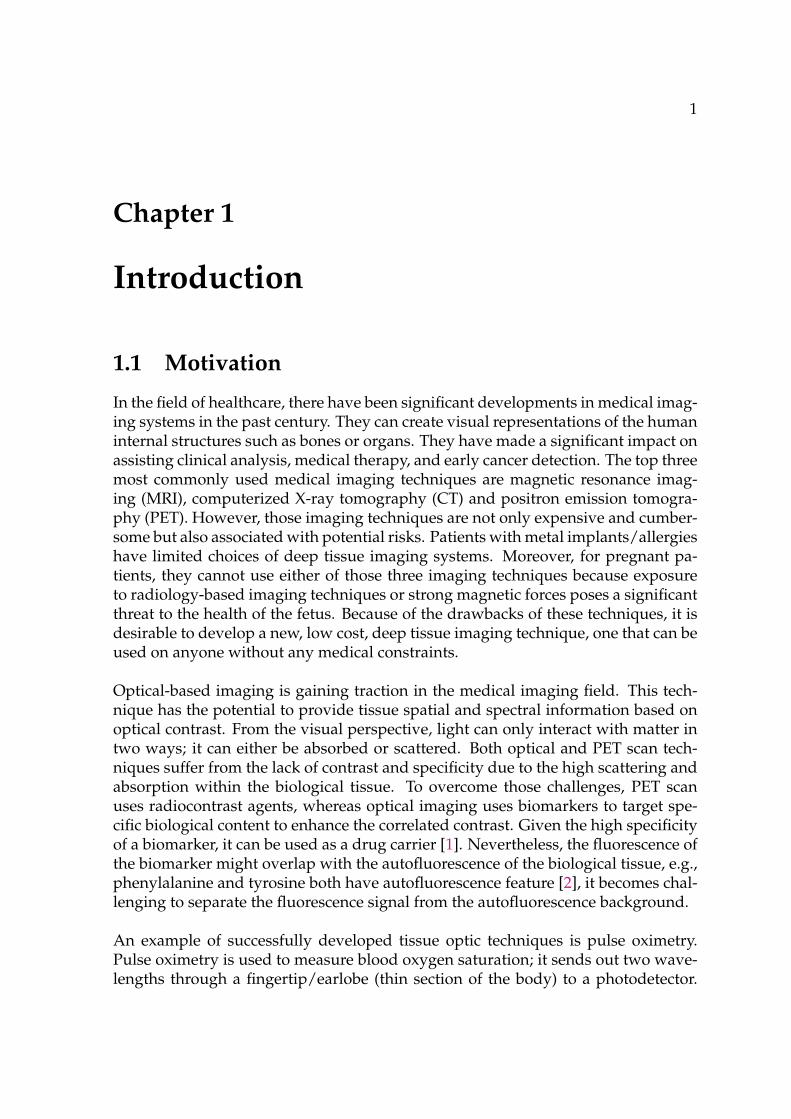
1.1 Motivation
In the field of healthcare, there have been significant developments in medical imag-ing systems in the past century. They can create visual representations of the humaninternal structures such as bones or organs. They have made a significant impact onassisting clinical analysis, medical therapy, and early cancer detection. The top threemost commonly used medical imaging techniques are magnetic resonance imag-ing (MRI), computerized X-ray tomography (CT) and positron emission tomogra-phy (PET). However, those imaging techniques are not only expensive and cumber-some but also associated with potential risks. Patients with metal implants/allergieshave limited choices of deep tissue imaging systems. Moreover, for pregnant pa-tients, they cannot use either of those three imaging techniques because exposureto radiology-based imaging techniques or strong magnetic forces poses a significantthreat to the health of the fetus. Because of the drawbacks of these techniques, it isdesirable to develop a new, low cost, deep tissue imaging technique, one that can beused on anyone without any medical constraints.
Optical-based imaging is gaining traction in the medical imaging field. This tech-nique has the potential to provide tissue spatial and spectral information based onoptical contrast. From the visual perspective, light can only interact with matter intwo ways; it can either be absorbed or scattered. Both optical and PET scan tech-niques suffer from the lack of contrast and specificity due to the high scattering andabsorption within the biological tissue. To overcome those challenges, PET scanuses radiocontrast agents, whereas optical imaging uses biomarkers to target spe-cific biological content to enhance the correlated contrast. Given the high specificityof a biomarker, it can be used as a drug carrier [1]. Nevertheless, the fluorescence ofthe biomarker might overlap with the autofluorescence of the biological tissue, e.g.,phenylalanine and tyrosine both have autofluorescence feature [2], it becomes chal-lenging to separate the fluorescence signal from the autofluorescence background.
An example of successfully developed tissue optic techniques is pulse oximetry.Pulse oximetry is used to measure blood oxygen saturation; it sends out two wave-lengths through a fingertip/earlobe (thin section of the body) to a photodetector.
2 Chapter 1. Introduction
Different variants of tissues exhibit different optical properties. For example, oxy-genated and deoxygenated hemoglobin would absorb different amounts of lightat the same wavelength. Tumorous tissues have different biological compositionsfrom the surrounding healthy tissue, which means their optical properties are sig-nificantly different. If the optical-based imaging is capable of distinguishing differ-ent biological contents based on collected optical information, it has the potentialto perform deep tissue imaging based on optical contrast. However, the light thatcomes out of the tissue encounters multiple scattering and absorption events, andthere is no way of reconstructing where and when the light underwent changes in-side the tissue. To enhance the correlated contrast for optical imaging techniquewithout invasiveness (the injection of biomarker), it requires the assistance of otherimaging technique. One idea involves the ultrasound imaging technique. The ultra-sound can penetrate deep into the tissue with a relatively high mechanical contrastremain.
1.2 Aim
The aim of this thesis is developing an ultrasound optical tomography (UOT) tech-nique, seek to keep the advantages of both optical and ultrasound imaging methodsand overcome both their limitations. The principle of UOT is tagging the photonsinside the medium with focused ultrasound, the ultrasound modulates the mediumrefractive index and turns it into a phase and amplitude grating. Light diffractedon the grating is frequency shifted by one or multiples of the ultrasound frequency.The light irradiance in the medium can be mapped out by monitoring the taggedphotons’ intensity while moving the ultrasound focus. The UOT should be able topenetrate deep enough to reach the heart or brain with sufficient contrast-to-noiseratio to measure the blood oxygen saturation [3]. UOT has the potential to acquireimages of the interior aspect of the body in a much shorter time than MRI and CT.Meanwhile, UOT does not require radiotracers (meaning the hospital does not needto have a particle accelerator like a cyclotron) nor operate in a strong magnetic fieldenvironment (MRI requires superconducting magnets). In an ideal situation, thepatient can frequently have an early stroke or tumor/cancer health check beforesymptoms appear, offering patients a higher survival rate compared to the late-stagediagnose.
3
Chapter 2
Theoretical Background
2.1 Light-tissue interactions, scattering and absorption
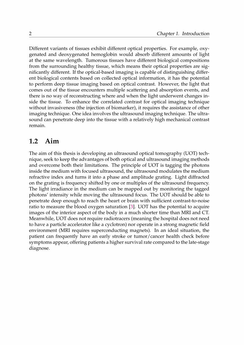
When light interacts with biological tissue, due to the higher refractive index of thetissue medium, Fresnel reflection will happen at the interface, while the rest of thelight would penetrate the tissue. As shown in figure 2.1, the light beam dispersesand disappears as the light penetrates deeper. Heat can be generated when mediumabsorbs the light. Once the medium cools down, the relaxation of the mediumwould generate acoustic waves. There are also special materials that can cause aut-ofluorescence or fluorescence under specific environmental conditions. Scattering(quantified by µs) and absorption (quantified by µa) of the medium are the mostresponsible properties for the redistribution of light.
FIGURE 2.1: Multiple events are involved in a light-tissue interaction, light is redistributedbased on the optical properties of the medium.
4 Chapter 2. Theoretical Background
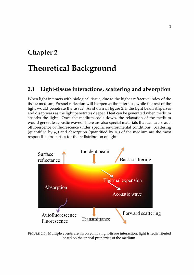
2.1.1 Scattering coefficientBiological tissue is a highly scattering medium. Each particle inside the tissue ismodeled as a homogeneous spherical structure with high refractive index[4] to sim-plify the simulation and calculation. The scattering coefficient µs is defined as theprobability per unit length a photon scatters, and it is characterized by a scatteringphase function. Few parameters are involved in the phase function to describe ascattering process: θ is the scattering angle in the scattering plane (angle betweenz-axis and ~S1), and ϕ is the scattering angle in the x-y plane (angle between x-axisand ~E‖i), see figure 2.2. The phase function is usually denoted as p(θ, ϕ), p representsthe probability density function for the process where a scattered photon change itstrajectory.
FIGURE 2.2: Geometry illustration of the scattering phase function, image cited from [5]. ~S0is the incident beam direction which is parallel to the z-axis, and ~S1 is the scattered lightdirection. On the scattering plane, the two orthogonal polarization components of the scat-tering lights are presented as vectors ~E‖s and ~E⊥s, and their projections on the x-y plane are
presented as vectors ~E‖i and ~E⊥i.
The phase function can be simplified and rewritten as p(θ) when the scattering issymmetric relative to the incident beam, and the phase function is then only depen-dent on the scattering angle θ. In the figure above, the trajectory of the scatteredphoton in the z-axis is presented as cos(θ). There are two scattering types. Rayleigh
2.1. Light-tissue interactions, scattering and absorption 5
scattering happens when the scattering particle size is way smaller than the incom-ing wavelength, such scattering event is highly wavelength dependent and mostlyisotropic. Mie scattering happens when the particle size is larger than the incidentwavelength, it is no longer isotropic, and it is mostly in the forward direction (closeto the incident beam direction). Mie scattering dominates the light-tissue interac-tion [4]. The averaged scattering direction is denoted by symbol g, and it is calledthe anisotropy factor:
g =< cos θ >=∫ π
0p(θ) cos θ · 2π sin θdθ. (2.1)
g factor is only used in medical optics to describe the angular distribution of scat-tered light. For an isotropic Rayleigh scattering, the g factor equals 0, and the scat-tering events are identically distributed in all directions. When the g value variesfrom -1 to 1, it represents a Mie scattering event. When g equals 1 the particle scat-ters forward, and when g equals -1 the particle scatters backward. Combining the gfactor and µs, the reduced scattering coefficient µ′s can be quantified:
µ′s = µs(1− g). (2.2)
Reduced scattering coefficient represents the diffusion of a photon within the mediumwhere every step is isotropic scattering. When g equals 1, reduced scattering coef-ficient becomes 0, meaning the incident photon remains its initial direction, there isnot scattering event and no losses of information.
During this thesis work, Intralipid 20% from Fresenius Kabi AB was used as a scat-terer. Intralipid is also known as lipid emulsion, and it is a medical product that con-sists of small droplets of fat within the water. Mixture a small percent of intralipidwith water would form a highly scattering suspension. Intralipid uniformity wasexamined by Di Ninni et al[6], the batch to batch variation is 2% for intralipid’sreduced scattering coefficient, and its absorption coefficient is minimal and can betreated as equal to the one of water. Since Intralipid is a diffusive reference standardfor optical phantoms, it has a known scattering coefficient. René Michels et al. [7]calculated the reduced scattering coefficient for intralipid 20% by fitting to the Mietheory from 400 nm to 900 nm,
µ′s(λ) = y0 + a · λ+ b · λ2 [mm−1/(ml/l)], (2.3)
where the wavelength λ is in nanometers, other parameters y0 = 8.261E+1, a = -1.288E-1, and b = 6.093E-5 [7], the unit of µs’ is interpreted as mm−1 per ml intralipid20% per l of total diluted suspension .
6 Chapter 2. Theoretical Background
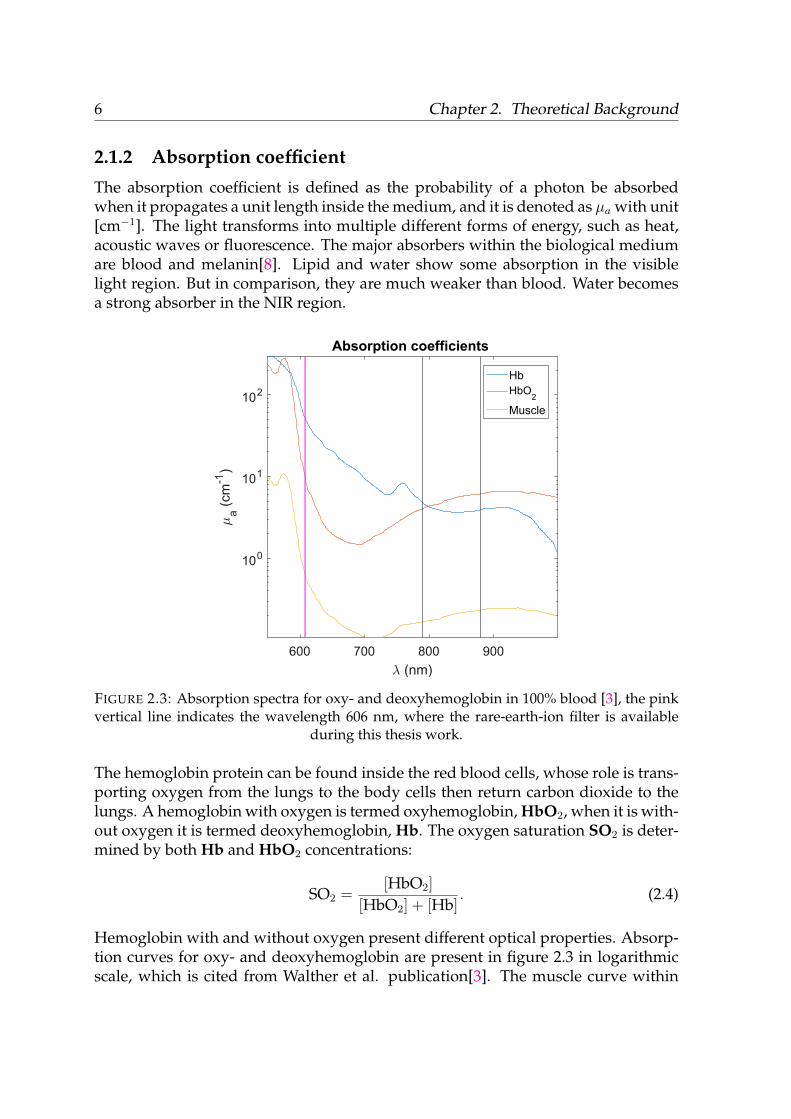
2.1.2 Absorption coefficientThe absorption coefficient is defined as the probability of a photon be absorbedwhen it propagates a unit length inside the medium, and it is denoted as µa with unit[cm−1]. The light transforms into multiple different forms of energy, such as heat,acoustic waves or fluorescence. The major absorbers within the biological mediumare blood and melanin[8]. Lipid and water show some absorption in the visiblelight region. But in comparison, they are much weaker than blood. Water becomesa strong absorber in the NIR region.
FIGURE 2.3: Absorption spectra for oxy- and deoxyhemoglobin in 100% blood [3], the pinkvertical line indicates the wavelength 606 nm, where the rare-earth-ion filter is available
during this thesis work.
The hemoglobin protein can be found inside the red blood cells, whose role is trans-porting oxygen from the lungs to the body cells then return carbon dioxide to thelungs. A hemoglobin with oxygen is termed oxyhemoglobin, HbO2, when it is with-out oxygen it is termed deoxyhemoglobin, Hb. The oxygen saturation SO2 is deter-mined by both Hb and HbO2 concentrations:
SO2 =[HbO2]
[HbO2] + [Hb]. (2.4)
Hemoglobin with and without oxygen present different optical properties. Absorp-tion curves for oxy- and deoxyhemoglobin are present in figure 2.3 in logarithmicscale, which is cited from Walther et al. publication[3]. The muscle curve within
2.2. Light propagation within the tissue 7
the figure assumes a normal muscle tissue containing 4% of blood and 85% oxygensaturation.
Talens Indian ink purchased from Svenskt Konstnärscentrum was used as the ab-sorber. However, unlike intralipid, ink does not have a controlled production con-dition, its absorption coefficient varies between brands and batches. Thus, the ab-sorption coefficient of our Indian ink will be measured and discussed in followingchapters.
2.2 Light propagation within the tissue
The previous section discussed scattering and absorption from the view of a sin-gle photon. However, after light entered tissue, the photons experience multiplescattering and absorption events, which make optical-based imaging in deep tissuechallenging. After several random scattering and absorption interactions, light in-formation such as polarization or phase is lost for diffused photons, and it becomesvery challenging to retrace the photons trajectories within the medium.
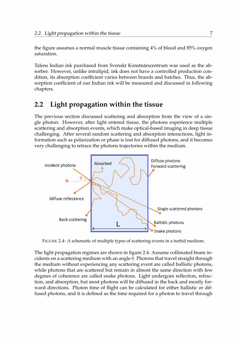
FIGURE 2.4: A schematic of multiple types of scattering events in a turbid medium.
The light propagation regimes are shown in figure 2.4. Assume collimated beam in-cidents on a scattering medium with an angle θ. Photons that travel straight throughthe medium without experiencing any scattering event are called ballistic photons,while photons that are scattered but remain in almost the same direction with fewdegrees of coherence are called snake photons. Light undergoes reflection, refrac-tion, and absorption, but most photons will be diffused in the back and mostly for-ward directions. Photon time of flight can be calculated for either ballistic or dif-fused photons, and it is defined as the time required for a photon to travel through
8 Chapter 2. Theoretical Background
a distance L inside a turbid medium[9] :
TOF =L
cosθ + ∆L
v, (2.5)
where v is the speed of light inside the medium, θ is the beam propagating angle, L isthe thickness of the medium and ∆L is the increased photon path due to scattering.
2.2.1 Monte Carlo simulation
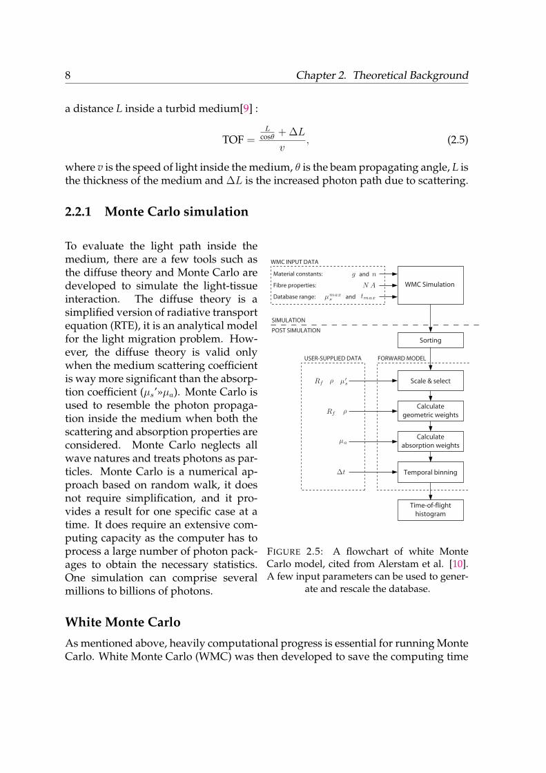
FIGURE 2.5: A flowchart of white MonteCarlo model, cited from Alerstam et al. [10].A few input parameters can be used to gener-
ate and rescale the database.
To evaluate the light path inside themedium, there are a few tools such asthe diffuse theory and Monte Carlo aredeveloped to simulate the light-tissueinteraction. The diffuse theory is asimplified version of radiative transportequation (RTE), it is an analytical modelfor the light migration problem. How-ever, the diffuse theory is valid onlywhen the medium scattering coefficientis way more significant than the absorp-tion coefficient (µs’»µa). Monte Carlo isused to resemble the photon propaga-tion inside the medium when both thescattering and absorption properties areconsidered. Monte Carlo neglects allwave natures and treats photons as par-ticles. Monte Carlo is a numerical ap-proach based on random walk, it doesnot require simplification, and it pro-vides a result for one specific case at atime. It does require an extensive com-puting capacity as the computer has toprocess a large number of photon pack-ages to obtain the necessary statistics.One simulation can comprise severalmillions to billions of photons.
White Monte CarloAs mentioned above, heavily computational progress is essential for running MonteCarlo. White Monte Carlo (WMC) was then developed to save the computing time
2.2. Light propagation within the tissue 9
[11] [12], one simulation of WMC is a combination of a wide range of optical prop-erties with proper rescaling [10]. The light paths are only determined by the phasescattering function and a sequence of random numbers [10] in a non-absorptive ho-mogeneously turbid medium. The scheme in figure 2.5 illustrates the WMC model.Users can input few parameters to generate a database, that include the materialanisotropy factor g, the refractive index n, the fiber numerical aperture NA, themaximum scattering level µmaxs for the simulation and the stop time tmax. Then thedatabase is sorted and stored and sent to the forward model. Based on the user inputparameters for the forward model, the database is then rescaled, and a correspond-ing time of flight histogram is generated. Those parameters are the radius Rf of theincoming beam, separation distance between detector and source ρ, reduced scatter-ing coefficient µ′s, absorption coefficient µa and desired temporal channel width ∆t[10][13]. During this thesis work, the databases were compiled by previous Biopho-tonics group members for intralipid in an infinite geometry[10]. The photons weresimulated at µs = µmaxs = 90 cm−1, µa = 0 cm−1, tmax = 2 ns, NA = 0.29, n = 1.33, g= 0.70 and 2×10⁸ photons. Photons are terminated in the simulation if the time offlight exceeds the tmax or they left the medium.
2.2.2 Photon time of flight spectroscopy
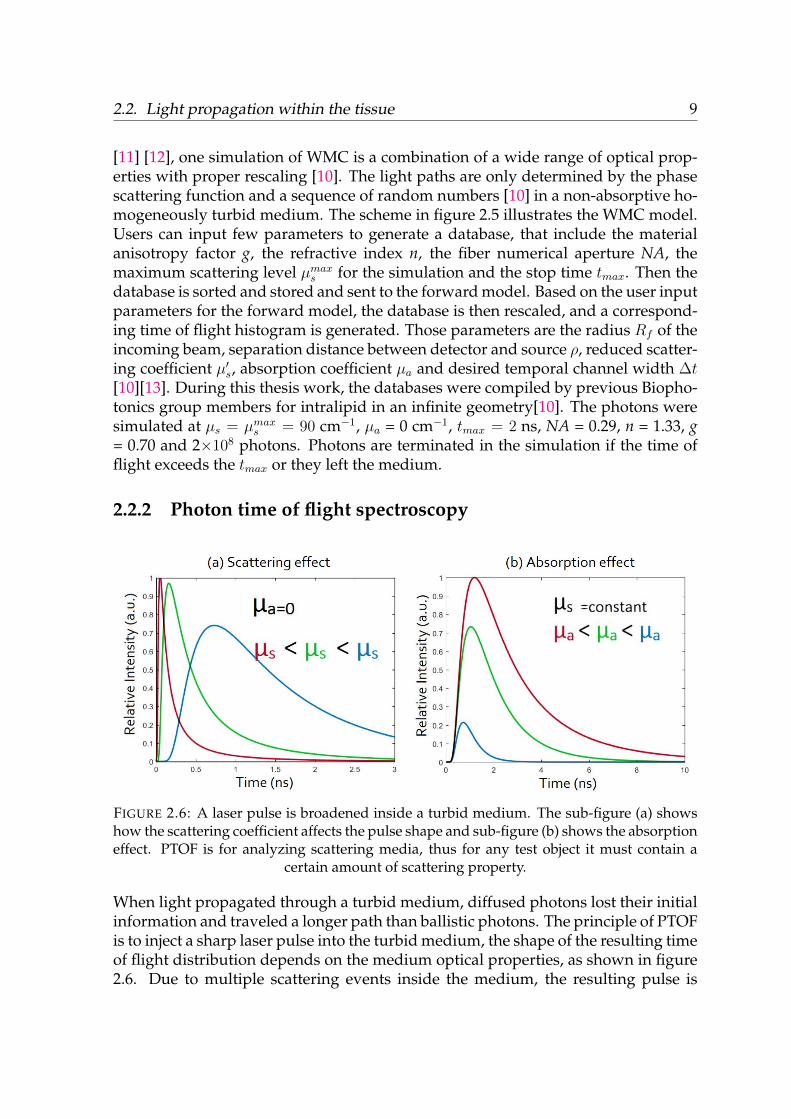
FIGURE 2.6: A laser pulse is broadened inside a turbid medium. The sub-figure (a) showshow the scattering coefficient affects the pulse shape and sub-figure (b) shows the absorptioneffect. PTOF is for analyzing scattering media, thus for any test object it must contain a
certain amount of scattering property.
When light propagated through a turbid medium, diffused photons lost their initialinformation and traveled a longer path than ballistic photons. The principle of PTOFis to inject a sharp laser pulse into the turbid medium, the shape of the resulting timeof flight distribution depends on the medium optical properties, as shown in figure2.6. Due to multiple scattering events inside the medium, the resulting pulse is
10 Chapter 2. Theoretical Background
much broader than the initial pulse. Increase the scattering coefficient would causethe photons undergo more scattering events, the average photons take a longer path,cause the peak of PTOF signal profile shifts to the later time (to the right in figure2.6). More scattering events meaning more photons could be absorbed during thepropagation, thus the peak intensity would decrease. Increase the absorption coeffi-cient will increase the absorption rate and lower the light intensity, the PTOF profileshifts to the earlier time (to the left in figure 2.6) as more late photons are absorbed.
However, to record the profile of delayed pulse in one cycle is very challenging. Thelaser pulse width used for PTOF is usually in picoseconds scale. To be able to resolvethe photon distribution, the detector must be extremely fast to such an extent. Sucha detector is very costly and does not have an excellent temporal resolution. Insteadof performing a direct pulse profile recording, a technique name time-correlatedsingle photon counting (TCSPC) was used, it is also known as photon time of flightspectroscopy. In this technique multiple short laser pulses are sent into to a turbidsample, a single or no photon is registered for each pulse at the detector to buildup a photon arrival time histogram. The profile of the histogram represents thelaser pulse broadening. By fitting the broadened pulse with the database, the turbidmedium absorption and scattering information can be extracted.
2.3 Ultrasound optical tomography
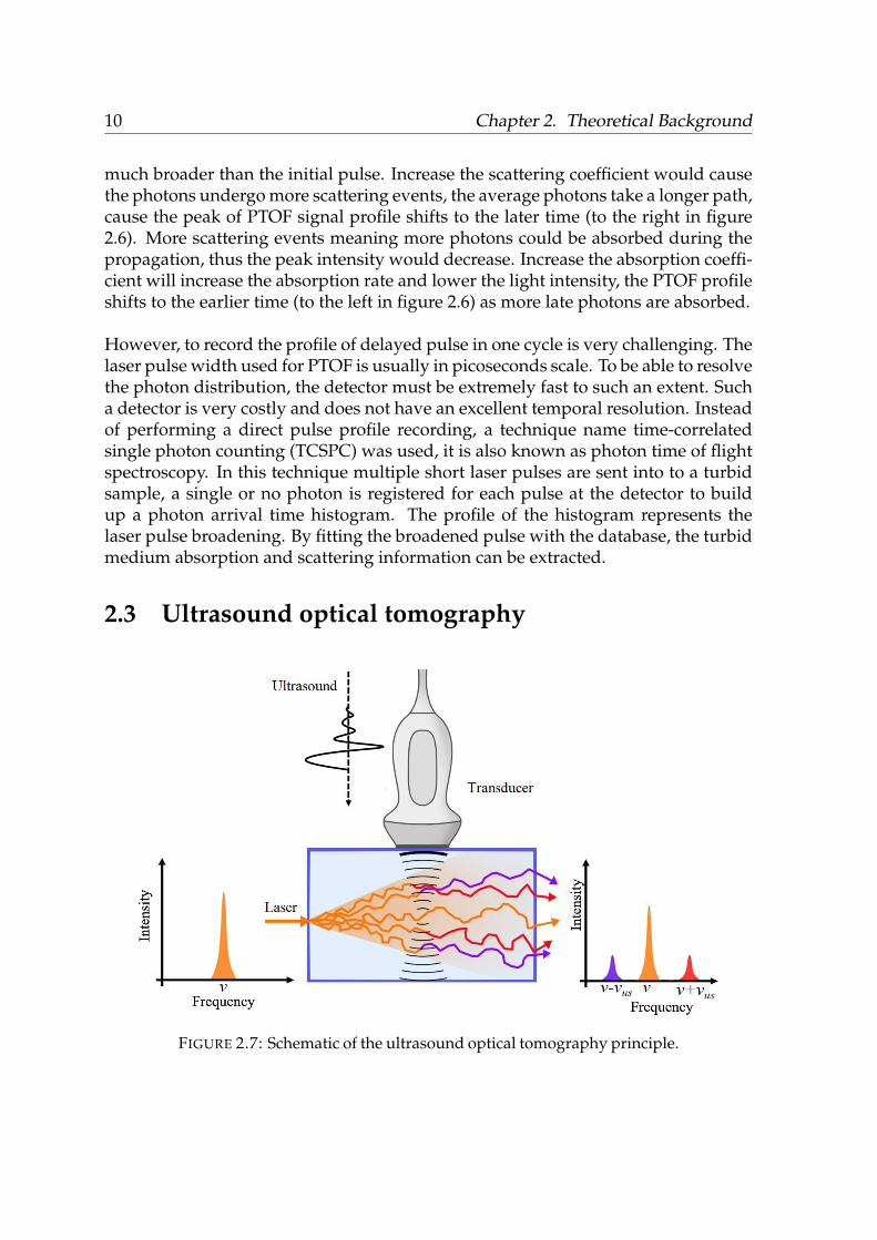
FIGURE 2.7: Schematic of the ultrasound optical tomography principle.
2.3. Ultrasound optical tomography 11
Ultrasound optical tomography is based on the acousto-optic effect. When an ul-trasound is applied to a biological tissue, see figure 2.7, the ultrasound wave willmodulate the refractive index of the medium and turn it into a phase and ampli-tude grating. For any incoming light diffracted on the grating, the diffracted lightfrequency is shifted by one or multiples of ultrasound frequency. The first ordersideband (two frequency bands on either side of the carrier wave) shifted by one ul-trasound frequency contains the most number of modulated photons, those photonsare named the tagged photons. Tagged photons intensity is dependent on the targetoptical properties, and the focused ultrasound volume indicates the origin of thesetagged photons[14]. It is possible to map the light spatial distribution within themedium by scanning the ultrasound focus, the resolution of the map is dependenton the ultrasound focus size.
2.3.1 Ultrasound and focus
A commercial ultrasound machine EPIQ7 from Philips was borrowed from Biomed-ical Engineering, LTH. Ultrasound is a sound wave in a high-frequency region thatexcesses the upper audible limit of human hearing.
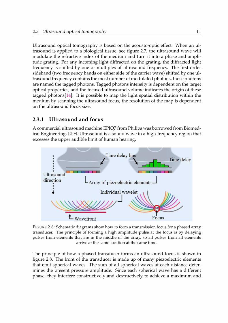
FIGURE 2.8: Schematic diagrams show how to form a transmission focus for a phased arraytransducer. The principle of forming a high amplitude pulse at the focus is by delayingpulses from elements that are in the middle of the array, so all pulses from all elements
arrive at the same location at the same time.
The principle of how a phased transducer forms an ultrasound focus is shown infigure 2.8. The front of the transducer is made up of many piezoelectric elementsthat emit spherical waves. The sum of all spherical waves at each distance deter-mines the present pressure amplitude. Since each spherical wave has a differentphase, they interfere constructively and destructively to achieve a maximum and
12 Chapter 2. Theoretical Background
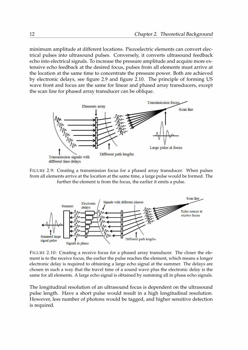
minimum amplitude at different locations. Piezoelectric elements can convert elec-trical pulses into ultrasound pulses. Conversely, it converts ultrasound feedbackecho into electrical signals. To increase the pressure amplitude and acquire more ex-tensive echo feedback at the desired focus, pulses from all elements must arrive atthe location at the same time to concentrate the pressure power. Both are achievedby electronic delays, see figure 2.9 and figure 2.10. The principle of forming USwave front and focus are the same for linear and phased array transducers, exceptthe scan line for phased array transducer can be oblique.
FIGURE 2.9: Creating a transmission focus for a phased array transducer. When pulsesfrom all elements arrive at the location at the same time, a large pulse would be formed. The
further the element is from the focus, the earlier it emits a pulse.
FIGURE 2.10: Creating a receive focus for a phased array transducer. The closer the ele-ment is to the receive focus, the earlier the pulse reaches the element, which means a longerelectronic delay is required to obtaining a large echo signal at the summer. The delays arechosen in such a way that the travel time of a sound wave plus the electronic delay is thesame for all elements. A large echo signal is obtained by summing all in phase echo signals.
The longitudinal resolution of an ultrasound focus is dependent on the ultrasoundpulse length. Have a short pulse would result in a high longitudinal resolution.However, less number of photons would be tagged, and higher sensitive detectionis required.
2.3. Ultrasound optical tomography 13
2.3.2 Acousto-optics
) 1
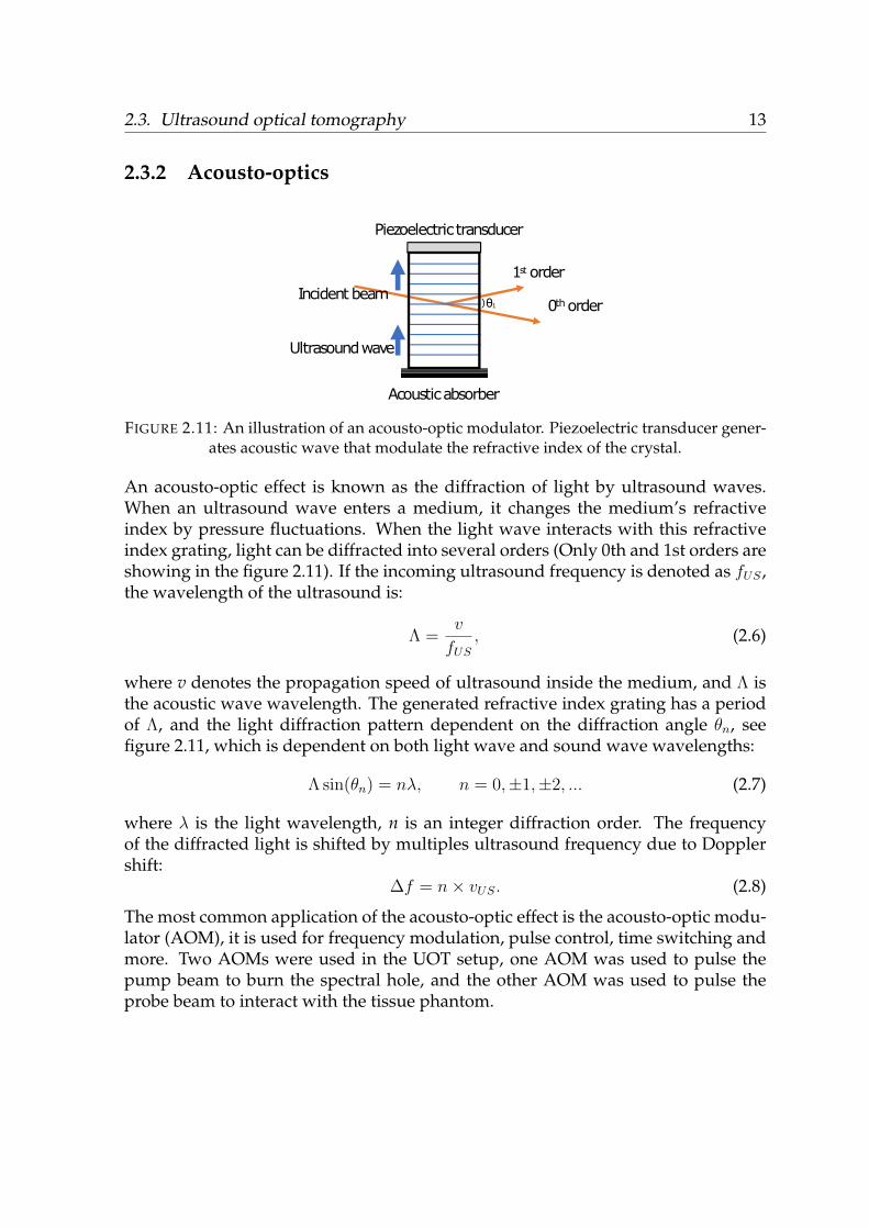
FIGURE 2.11: An illustration of an acousto-optic modulator. Piezoelectric transducer gener-ates acoustic wave that modulate the refractive index of the crystal.
An acousto-optic effect is known as the diffraction of light by ultrasound waves.When an ultrasound wave enters a medium, it changes the medium’s refractiveindex by pressure fluctuations. When the light wave interacts with this refractiveindex grating, light can be diffracted into several orders (Only 0th and 1st orders areshowing in the figure 2.11). If the incoming ultrasound frequency is denoted as fUS ,the wavelength of the ultrasound is:
Λ =v
fUS, (2.6)
where v denotes the propagation speed of ultrasound inside the medium, and Λ isthe acoustic wave wavelength. The generated refractive index grating has a periodof Λ, and the light diffraction pattern dependent on the diffraction angle θn, seefigure 2.11, which is dependent on both light wave and sound wave wavelengths:
Λ sin(θn) = nλ, n = 0,±1,±2, ... (2.7)
where λ is the light wavelength, n is an integer diffraction order. The frequencyof the diffracted light is shifted by multiples ultrasound frequency due to Dopplershift:
∆f = n× vUS. (2.8)
The most common application of the acousto-optic effect is the acousto-optic modu-lator (AOM), it is used for frequency modulation, pulse control, time switching andmore. Two AOMs were used in the UOT setup, one AOM was used to pulse thepump beam to burn the spectral hole, and the other AOM was used to pulse theprobe beam to interact with the tissue phantom.
14 Chapter 2. Theoretical Background
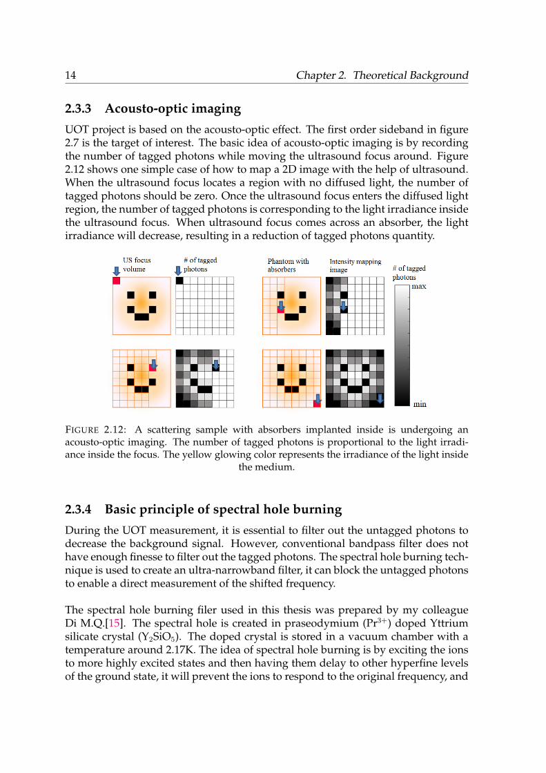
2.3.3 Acousto-optic imagingUOT project is based on the acousto-optic effect. The first order sideband in figure2.7 is the target of interest. The basic idea of acousto-optic imaging is by recordingthe number of tagged photons while moving the ultrasound focus around. Figure2.12 shows one simple case of how to map a 2D image with the help of ultrasound.When the ultrasound focus locates a region with no diffused light, the number oftagged photons should be zero. Once the ultrasound focus enters the diffused lightregion, the number of tagged photons is corresponding to the light irradiance insidethe ultrasound focus. When ultrasound focus comes across an absorber, the lightirradiance will decrease, resulting in a reduction of tagged photons quantity.
FIGURE 2.12: A scattering sample with absorbers implanted inside is undergoing anacousto-optic imaging. The number of tagged photons is proportional to the light irradi-ance inside the focus. The yellow glowing color represents the irradiance of the light inside
the medium.
2.3.4 Basic principle of spectral hole burningDuring the UOT measurement, it is essential to filter out the untagged photons todecrease the background signal. However, conventional bandpass filter does nothave enough finesse to filter out the tagged photons. The spectral hole burning tech-nique is used to create an ultra-narrowband filter, it can block the untagged photonsto enable a direct measurement of the shifted frequency.
The spectral hole burning filer used in this thesis was prepared by my colleagueDi M.Q.[15]. The spectral hole is created in praseodymium (Pr3+) doped Yttriumsilicate crystal (Y2SiO5). The doped crystal is stored in a vacuum chamber with atemperature around 2.17K. The idea of spectral hole burning is by exciting the ionsto more highly excited states and then having them delay to other hyperfine levelsof the ground state, it will prevent the ions to respond to the original frequency, and
2.3. Ultrasound optical tomography 15
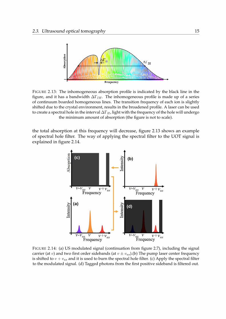
FIGURE 2.13: The inhomogeneous absorption profile is indicated by the black line in thefigure, and it has a bandwidth ∆ΓIH . The inhomogeneous profile is made up of a seriesof continuum boarded homogeneous lines. The transition frequency of each ion is slightlyshifted due to the crystal environment, results in the broadened profile. A laser can be usedto create a spectral hole in the interval ∆ΓH , light with the frequency of the hole will undergo
the minimum amount of absorption (the figure is not to scale).
the total absorption at this frequency will decrease, figure 2.13 shows an exampleof spectral hole filter. The way of applying the spectral filter to the UOT signal isexplained in figure 2.14.
FIGURE 2.14: (a) US modulated signal (continuation from figure 2.7), including the signalcarrier (at v) and two first order sidebands (at v ± vus).(b) The pump laser center frequencyis shifted to v + vus and it is used to burn the spectral hole filter. (c) Apply the spectral filterto the modulated signal. (d) Tagged photons from the first positive sideband is filtered out.
16
Chapter 3
Experiment
3.1 Tissue-mimicking phantom preparation
Due to the complexity and risks of testing developing medical diagnostics on pa-tients, tissue models are developed to evaluate the theoretical predictions. It mim-ics the structural and optical properties of the actual biological objects. The moststraightforward approach of characterizing a tissue phantom with known opticalproperties is by mixing known proportions of pure scatterer and absorber.
3.1.1 Optical characterization of a homogeneous liquid phantom
The tissue model optical parameters should be able to be predicted by knowing thecompositions and constituents’ characteristics. The liquid phantom is the simplesttissue model to start with, and it has very high flexibility regarding changing theabsorption and scattering properties. Distilled water is used as the base for a liquidphantom, then the absorbers and scatterers are suspended in the water. Water istransparent and non-scattering, it has a relatively low absorption coefficient in thevisible wavelength region (at 606 nm, µa = 0.0026 cm−1[16]).
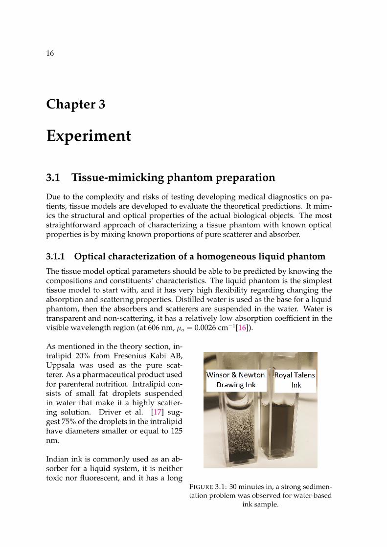
FIGURE 3.1: 30 minutes in, a strong sedimen-tation problem was observed for water-based
ink sample.
As mentioned in the theory section, in-tralipid 20% from Fresenius Kabi AB,Uppsala was used as the pure scat-terer. As a pharmaceutical product usedfor parenteral nutrition. Intralipid con-sists of small fat droplets suspendedin water that make it a highly scatter-ing solution. Driver et al. [17] sug-gest 75% of the droplets in the intralipidhave diameters smaller or equal to 125nm.
Indian ink is commonly used as an ab-sorber for a liquid system, it is neithertoxic nor fluorescent, and it has a long
3.1. Tissue-mimicking phantom preparation 17
preserving time. However, unlike intralipid, Indian ink does not have a controlledproduction condition, and there is no standard absorption coefficient of ink for anybrand or batch. Large ink particle scatters visible and near-infrared red light. Water-based ink has a very strong sedimentation problem. ’Waterproof’ Ink from RoyalTalens was used, it does not have the diffusion problem, but it was quite difficultto dissolve them in water. A pre-diluted batch solution (1:100) of the Royal Talensink was prepared to solve the problem. Meanwhile, 2 hours ultrasound bath wasalso applied to the pre-diluted (1:100) ink solution to break the large suspended inkparticles. In figure 3.1, two different types of ink solutions were prepared by thesame procedure and proportion. The sedimentation problem started appearing forwater-based ink (Winsor & Newton) after 10 minutes, while it took two weeks oreven longer for the waterproof ink to begin sedimenting.
Two different methods were used to determine the absorption coefficient of the pre-diluted ink solution (1:100). Collimated transmission spectroscopy (also known asthe absorption spectroscopy, ABS) was the first approach. Colleague Di M.Q.[15]performed the ABS experiment to determine the prepared ink solution (1:100) ab-sorption coefficient. Her experiment result suggests,
y = 0.933× x, (3.1)
where y is the ink absorption coefficient [cm−1] and x is the ink concentration intotal volume [%]. The photon time of flight spectroscopy was used as the secondapproach of determining the ink absorption coefficient, the detail of this method ispresenting in section 3.1.3. The measured ink absorption coefficient by these twodifferent methods were compared in the result section 4.1.1.
3.1.2 Convert liquid phantom to solid phantomA liquid phantom with known optical properties is prepared by mixing properamounts of intralipid and ink solution (1:100). The advantage of a liquid phantomis that its properties can be varied easily, and that probe/detector can move freelywithin the medium. However, a fluid form model cannot mimic the macroscopicgeometry of a tissue sample, and it cannot hold a physical shape as an individual.
Making a solid tissue mimic phantom would be a better approach. It can be more ge-ometrically complicated with impurities implanted. Particles inside the solid phan-tom would experience the minimum amount of sedimentation problem. A goodsolid phantom for the UOT should have controlled and stable optical and mechan-ical properties, a near perfect matching interface between impurity and the sur-rounding. Also, more important, it should be aqueous to enable ultrasound propa-gation inside with minimum amount of US power loss.
18 Chapter 3. Experiment
Agar powder (A7921, SIGMA) was used to convert the liquid phantom into solidform, and it forms a transparent aqueous gel with water. It can hold water togetheris due to the presence of hydrophilic groups in the polymer chain (OH, -COOH,-CONH2, y-SO3H [18]). Just like the liquid phantom, agar phantom optical prop-erties can also be predicted from the individual characteristics of scatterer and ab-sorber. Rinaldo C. et al. [19] suggest 1% of agar powder is enough for hardeningthe phantom, as higher concentration gives a high viscosity of the solution whichmakes it difficult to dissolve and mix the components.
3.1.2.1 Procedures
4 g of agar powder was mixed with 400 mL of distilled water in a glass beaker.To avoid inhomogeneous heating, a magnetic stirring bar was put inside the glassbeaker, and together they were water bathed in a larger beaker on a hot plate stirrer(AREX Digital CerAlTop). External digital thermoregulator was connected to thestirrer to provide direct temperature control. The mixture of agar and water washeated to 95 C, and the solution was stirred with the magnetic stirring bar at aconstant speed for 2 hours. The opening of the breaker was sealed off with an alu-minum foil to minimize evaporation, and the stirring speed was set to a reasonablehigh value without form bubbles or whirls. As the agar powder dissolved com-pletely, the mixture solution turned transparent. Then the heating was set to 45 C,the stirring continued. An appropriate amount of ink and intralipid were addedinto the agar solution when the temperature was around 45 C. After stirring for 30minutes, the heating was turned off, and the mixed agar solution was transferredinto a cylindrical mold and solidified at room temperature.
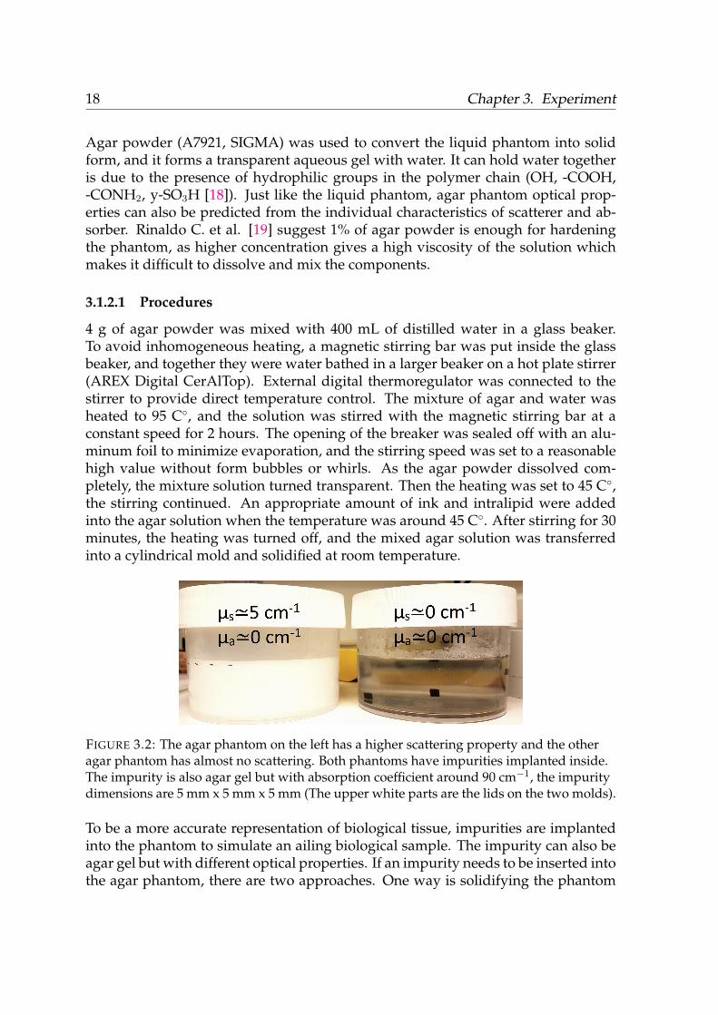
FIGURE 3.2: The agar phantom on the left has a higher scattering property and the otheragar phantom has almost no scattering. Both phantoms have impurities implanted inside.The impurity is also agar gel but with absorption coefficient around 90 cm−1, the impuritydimensions are 5 mm x 5 mm x 5 mm (The upper white parts are the lids on the two molds).
To be a more accurate representation of biological tissue, impurities are implantedinto the phantom to simulate an ailing biological sample. The impurity can also beagar gel but with different optical properties. If an impurity needs to be inserted intothe agar phantom, there are two approaches. One way is solidifying the phantom
3.1. Tissue-mimicking phantom preparation 19
layer by layer: pour a certain amount of mixture agar solution into the mold andlet it naturally hardens, while keeping stirring the rest solution in the water bath at45 C. Place the impurity on the solidified agar gel then carefully pour the rest ofsolution into the mold and let it cools at room temperature. This method is verytime consuming, but in exchange, the impurity is correctly placed at the desiredlocation. The second method is placing the impurity during the aqueous gel solidi-fying progress. A thin needle can be used to push the impurity from the surface ofthe solidifying gel into desired depth, the temperature of the mixture is generallyaround 38 C. This method is quick, but it requires to be good at judging the timing.If the gel is not viscous enough the impurity will not stay at the required location,if the gel surface is already solidified, forcing in the impurity would damage theinterface and structure. Using either of the methods must be careful in avoidingforming bubbles. The second method would not work well if the agar gel is highlyscattering or absorbing, as the impurity location optical information is lost duringmultiple scattering and absorption events, an example is presenting in figure 3.2.
All solidified phantoms should be sealed and stored in a water tank in a refrigerator(temperature around 10 C). The agar phantom can be used for measurement afterbeing cooled at least 12 hours. PTOF was also used to analyze the manufacturedagar phantom optical properties.
3.1.3 Photon time of flight spectroscopy
When a short laser pulse (on the picosecond scale) is sent into a scattering medium,the light experiences multiple scattering events, that cause the pulse profile broad-ened in time. By fitting the pulse curve with the WMC database, the optical prop-erties of the medium can be deduced. The optical properties of intralipid 20% andink base (1:100) were both examined by the PTOF spectroscopy. Since intralipid hasa standard reference value in scattering coefficient, the reduced scattering measure-ment result can also be used to test the precision and accuracy of PTOF.
3.1.3.1 Experimental Setup
A pulsed supercontinuum fiber laser (Model SC500-6, Fianium, UK) was used as thelight source, it has a repetition rate of 80 MHz, and it can generate 6.0 ps long pulses(500-1850 nm). The output light was coupled into an acousto-optic tunable filter(AOTF, SN101571). There are two crystals inside the AOTF housing; VIS crystalcovers the wavelength range 400-700 nm and NIR1 crystal covers the wavelengthrange 650-1100 nm. The acousto-optic tunable filter (AOTF) was used to select aspectrally narrow pulse, and the selected pulse bandwidth is about 3 nm when thewavelength is below 650 nm, and it increases to 6 nm at 1100 nm. A narrow-corefiber (10 µm, SMF-28) was coupled to the output of AOTF, and the light was sent toa beam splitter.
20 Chapter 3. Experiment
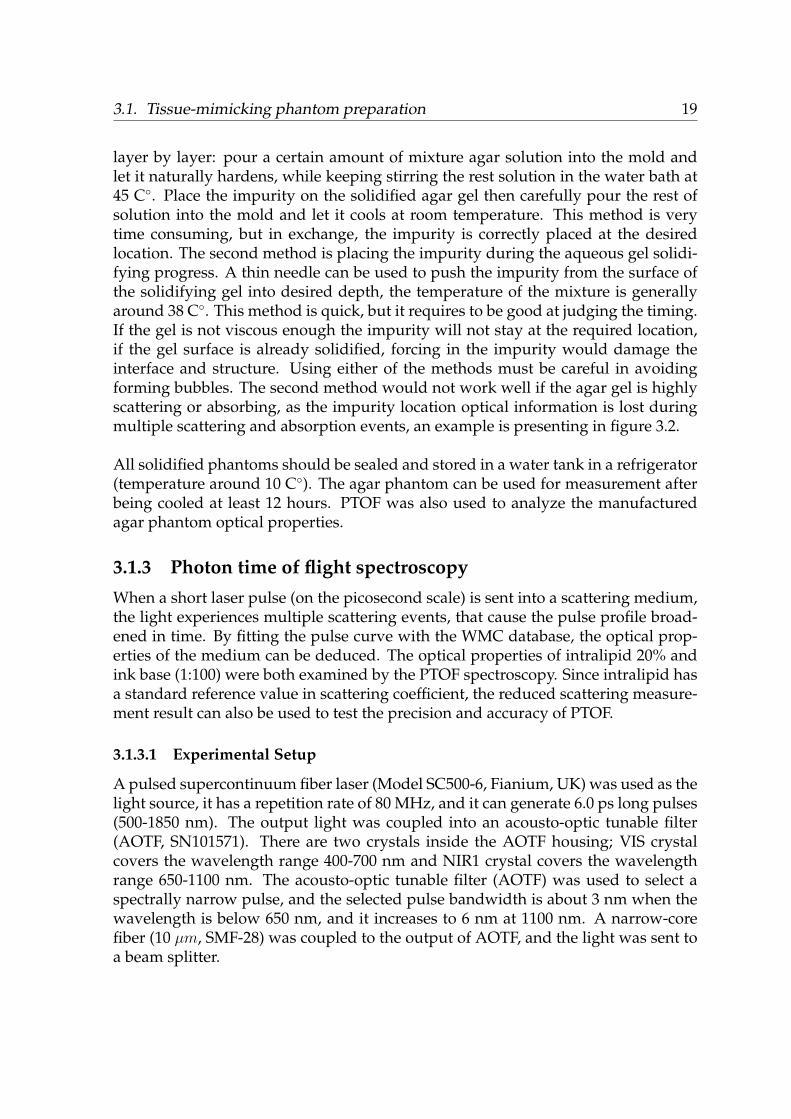
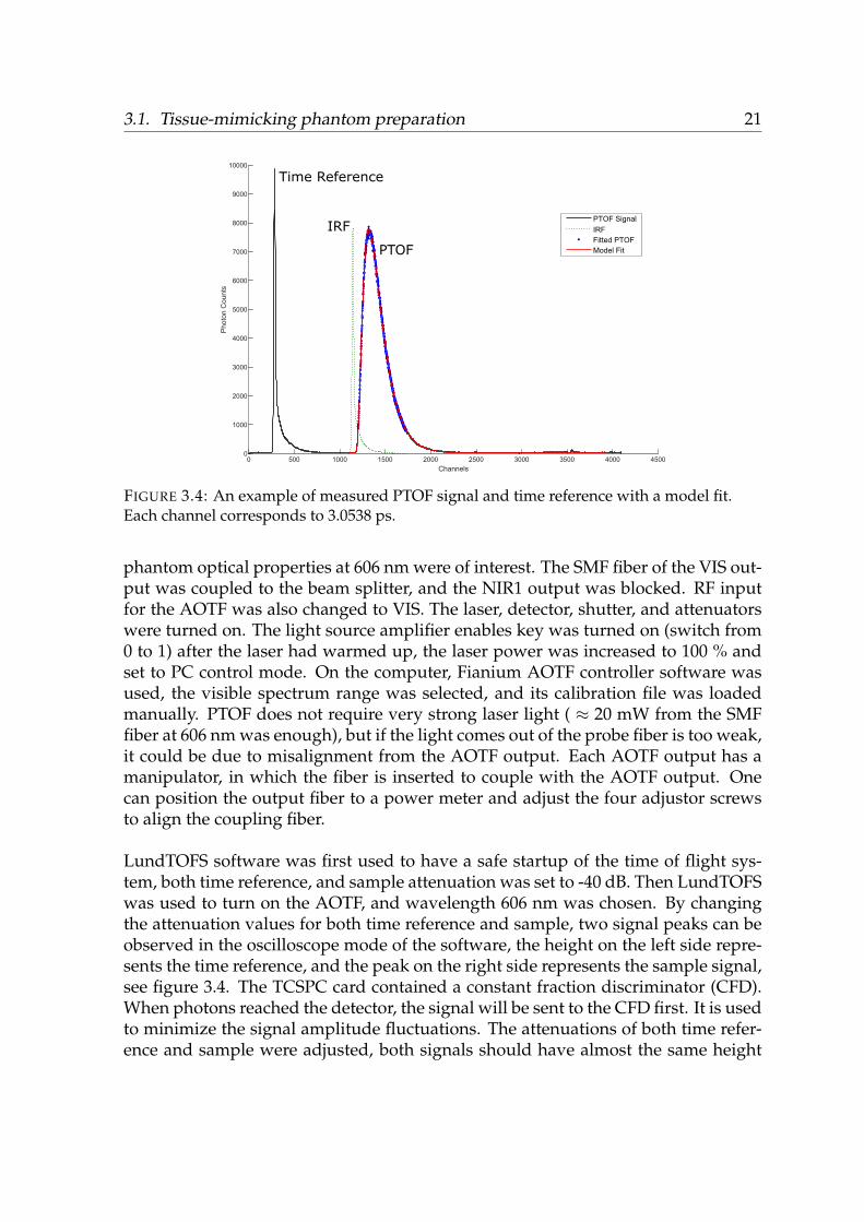
VIS: 400 to 700 nmNIR1: 650 to 1100 nm
FIGURE 3.3: Schematic arrangement of the PTOF setup. PTOF is capable of measuringsample absorption and reduced scattering coefficients the same time. If a light pulse is sentthrough a turbid medium, and the pulse will be broadened based on the statisticaldistribution of each detected photon’s optical path.
4% of the initial light pulse was severed as the time reference, and 96% of light wassent to the testing sample. Each beam path contains a variable optical attenuator(FVA-3100, OZ Optics Ltd), they were both remotely controlled by computer withinattenuation range -40 dB and -2.6 dB. Attenuators were used to adjust both beampaths pulse power to achieve single photon detection for the time of flight system.The 96% of light through the attenuator was coupled into a custom needle fiber. Theneedle fiber was inserted into the phantom, and the diffused light was collected bythe second needle fiber and combined with the reference light. Both needle fiberswere placed in parallel and kept at the same level. If a container was used to storethe tissue phantom, its wall must be covered by black tape or paper to minimize thereflection from the wall surface. The separation distance between the two fibers areadjustable, but usually, it was kept at 20 mm as the WMC database was calibratedfor a separation distance of 20 mm. The collected sample PTOF signal and the timereference pulse were combined at the beam combiner. A single photon countingavalanche photodiode detector (PD1CTC, Micro Photon Devices) was used for thevisible wavelength range detection. The APD was connected to a TCSPC card (SPC-130 Becker & Hickl, Berlin, Germany) to acquire the PTOF signal distribution.
3.1.3.2 Procedures
Depending on which wavelength is going to be used, the SMF fiber of VIS or NIR1should be coupled to the beam splitter. In this thesis work, the manufactured tissue
3.1. Tissue-mimicking phantom preparation 21
Time Reference
IRF
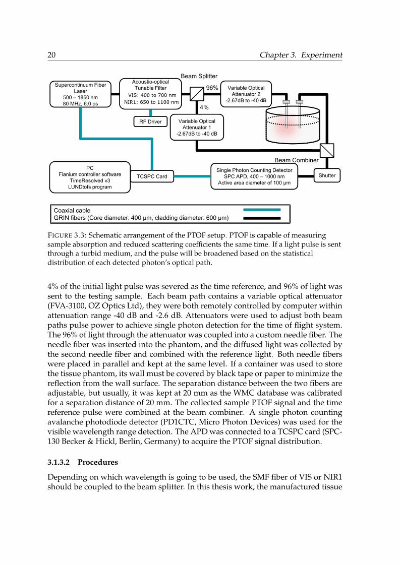
PTOF
FIGURE 3.4: An example of measured PTOF signal and time reference with a model fit.Each channel corresponds to 3.0538 ps.
phantom optical properties at 606 nm were of interest. The SMF fiber of the VIS out-put was coupled to the beam splitter, and the NIR1 output was blocked. RF inputfor the AOTF was also changed to VIS. The laser, detector, shutter, and attenuatorswere turned on. The light source amplifier enables key was turned on (switch from0 to 1) after the laser had warmed up, the laser power was increased to 100 % andset to PC control mode. On the computer, Fianium AOTF controller software wasused, the visible spectrum range was selected, and its calibration file was loadedmanually. PTOF does not require very strong laser light ( ≈ 20 mW from the SMFfiber at 606 nm was enough), but if the light comes out of the probe fiber is too weak,it could be due to misalignment from the AOTF output. Each AOTF output has amanipulator, in which the fiber is inserted to couple with the AOTF output. Onecan position the output fiber to a power meter and adjust the four adjustor screwsto align the coupling fiber.
LundTOFS software was first used to have a safe startup of the time of flight sys-tem, both time reference, and sample attenuation was set to -40 dB. Then LundTOFSwas used to turn on the AOTF, and wavelength 606 nm was chosen. By changingthe attenuation values for both time reference and sample, two signal peaks can beobserved in the oscilloscope mode of the software, the height on the left side repre-sents the time reference, and the peak on the right side represents the sample signal,see figure 3.4. The TCSPC card contained a constant fraction discriminator (CFD).When photons reached the detector, the signal will be sent to the CFD first. It is usedto minimize the signal amplitude fluctuations. The attenuations of both time refer-ence and sample were adjusted, both signals should have almost the same height
22 Chapter 3. Experiment
and their total photons counts per second should not exceed 1.0·105 photons/s. Af-ter finished the sample measurement, a double-sided thin black paper was insertedbetween two fibers, and this was used to perform the instrument response function(IRF) measurement. The incoming laser pulse is not infinitely narrow, and after ittraveled through multiple optical components the laser pulse was broadened (usu-ally≈ 80 ps). A thin piece of black paper has a relatively small amount of scattering,and it is used to mimic a tissue sample that has an extremely small temporal broad-ening.
Timeresolved v3 Matlab software was used to evaluate the absorption and reducedscattering coefficients of the acquired data. After both the IRF and sample files wereimported to the Timeresolved v3, the White Monte Carlo model was chosen. Dif-ferent data templates are available within the program, in this thesis work, tem-plate intralipid-finite.mat was used; the photons were simulated at µs = µmaxs = 90cm−1,µa = 0 cm−1, tmax = 2 ns, NA = 0.29, n = 1.33, g = 0.70 and 2×10⁸ photons.The 4% of the light fraction was used to sync the IRF and PTOF measurements thatwere taken at different times. The theoretical model was first convolved with theIRF pulse, and then the convolved pulse was used to try to fit with the broadenedPTOF pulse by iteration process of some combinations of µ′s and µa.
3.2 Ultrasound focus experimental setup
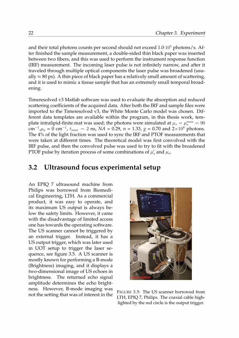
FIGURE 3.5: The US scanner borrowed fromLTH, EPIQ 7, Philips. The coaxial cable high-lighted by the red circle is the output trigger.
An EPIQ 7 ultrasound machine fromPhilips was borrowed from Biomedi-cal Engineering, LTH. As a commercialproduct, it was easy to operate, andits maximum US output is always be-low the safety limits. However, it camewith the disadvantage of limited accessone has towards the operating software.The US scanner cannot be triggered byan external trigger. Instead, it has aUS output trigger, which was later usedin UOT setup to trigger the laser se-quence, see figure 3.5. A US scanner ismostly known for performing a B-mode(Brightness) imaging, and it displays atwo-dimensional image of US echoes inbrightness. The returned echo signalamplitude determines the echo bright-ness. However, B-mode imaging wasnot the setting that was of interest in the
3.2. Ultrasound focus experimental setup 23
UOT project. Two US modes can form a US focus, M-mode (Motion display, com-monly used to view a mono-dimensional presentation of a heart) and PW-mode(Pulsed wave Doppler, commonly used to trace blood flow). Both modes have highrepetition rate. M-mode displays the chosen US line in time motion, PW-mode posi-tions the US focus at any point along the US line and detect the returned signal. Dueto background scanning (B-mode) cannot be stopped while running the M-modescan, PW-mode was used to assist the UOT project, and its US focus properties wereinvestigated.
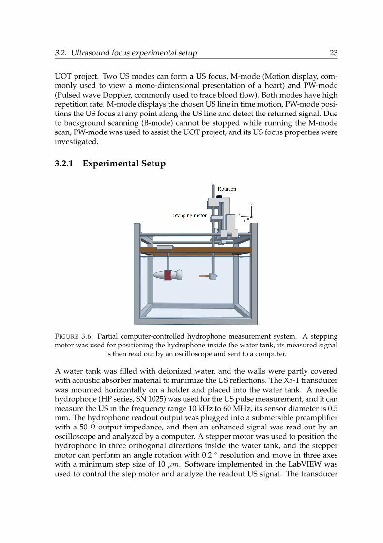
3.2.1 Experimental Setup
FIGURE 3.6: Partial computer-controlled hydrophone measurement system. A steppingmotor was used for positioning the hydrophone inside the water tank, its measured signal
is then read out by an oscilloscope and sent to a computer.
A water tank was filled with deionized water, and the walls were partly coveredwith acoustic absorber material to minimize the US reflections. The X5-1 transducerwas mounted horizontally on a holder and placed into the water tank. A needlehydrophone (HP series, SN 1025) was used for the US pulse measurement, and it canmeasure the US in the frequency range 10 kHz to 60 MHz, its sensor diameter is 0.5mm. The hydrophone readout output was plugged into a submersible preamplifierwith a 50 Ω output impedance, and then an enhanced signal was read out by anoscilloscope and analyzed by a computer. A stepper motor was used to position thehydrophone in three orthogonal directions inside the water tank, and the steppermotor can perform an angle rotation with 0.2 resolution and move in three axeswith a minimum step size of 10 µm. Software implemented in the LabVIEW wasused to control the step motor and analyze the readout US signal. The transducer
24 Chapter 3. Experiment
and hydrophone were first aligned, then the hydrophone was moved numericallyto measure the US amplitude distribution in a cross-section.
3.2.2 ProceduresThe most complicated and time-consuming part of the measurement procedure wasthe positioning and alignment of the transducer and hydrophone. As described inthe experimental setup, the transducer was mounted in a fixed position while thehydrophone was mounted on the stepper motor. The principle of the alignment was
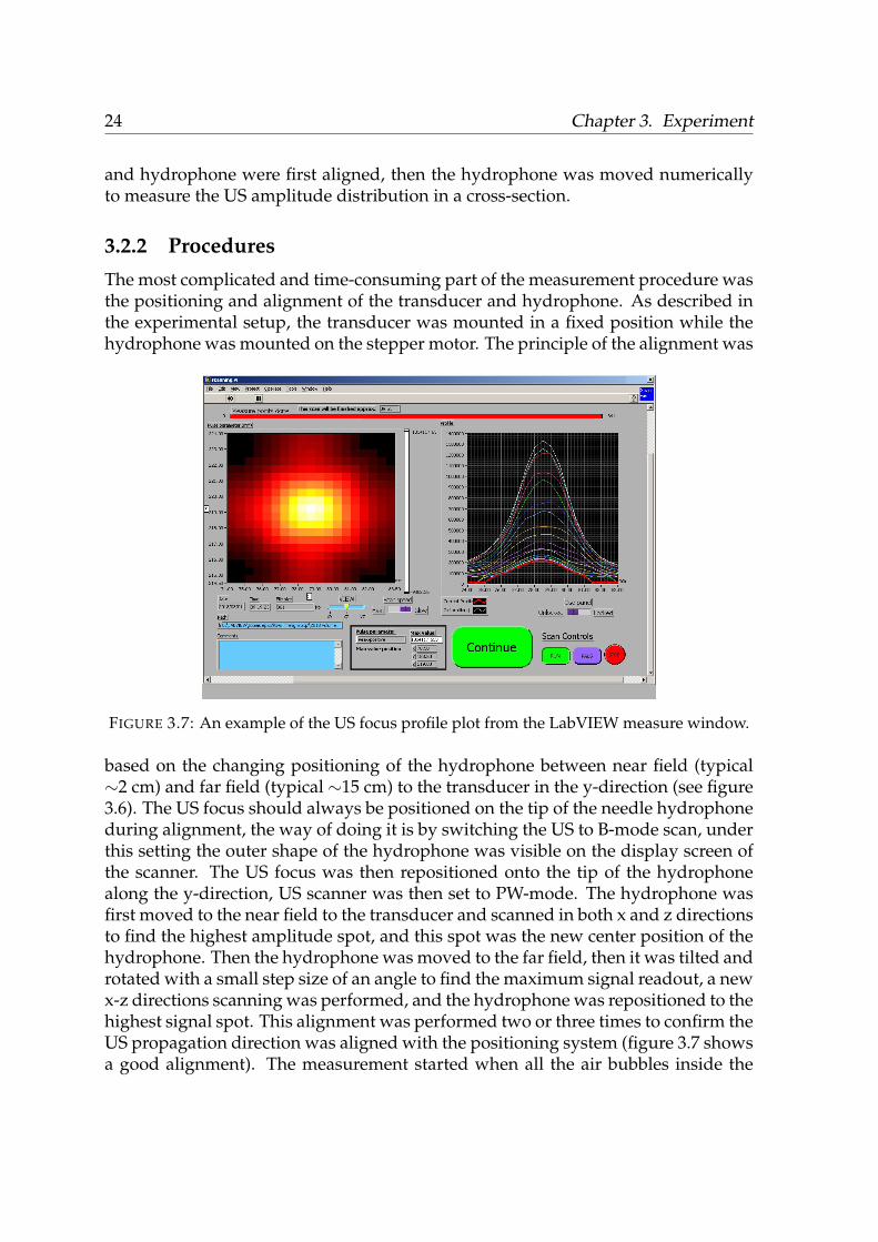
FIGURE 3.7: An example of the US focus profile plot from the LabVIEW measure window.
based on the changing positioning of the hydrophone between near field (typical∼2 cm) and far field (typical ∼15 cm) to the transducer in the y-direction (see figure3.6). The US focus should always be positioned on the tip of the needle hydrophoneduring alignment, the way of doing it is by switching the US to B-mode scan, underthis setting the outer shape of the hydrophone was visible on the display screen ofthe scanner. The US focus was then repositioned onto the tip of the hydrophonealong the y-direction, US scanner was then set to PW-mode. The hydrophone wasfirst moved to the near field to the transducer and scanned in both x and z directionsto find the highest amplitude spot, and this spot was the new center position of thehydrophone. Then the hydrophone was moved to the far field, then it was tilted androtated with a small step size of an angle to find the maximum signal readout, a newx-z directions scanning was performed, and the hydrophone was repositioned to thehighest signal spot. This alignment was performed two or three times to confirm theUS propagation direction was aligned with the positioning system (figure 3.7 showsa good alignment). The measurement started when all the air bubbles inside the
3.3. Ultrasound optical tomography 25
water tank is disappeared. For each pixel in figure 3.7 the full temporal profile ofthe US pulse is stored.
3.3 Ultrasound optical tomography
High scattering and high absorption properties of tissue limit most of the optic-based diagnostic methods. In contrast of UOT, US can penetrate deep into the tissue,but the laser intensity reaches the region of interest is relatively low, and the taggedlight from the small focused US volume are many orders of magnitude weaker thanthe carrier. A high finesse filter is a key to achieve the success of UOT development.Such a filter should have the highest possible etendue, sharp frequency edge, be sta-ble and long-lived (or permanent).
The optical transition 3H4 ⇒1 D2 of Praseodymium (Pr3+) ions in Pr3+:Y2SiO5 at2.17 K, 605.98 nm, was used to prepare the spectral filter by colleague Di M.Q.[15].606 nm is not an ideal wavelength for deep tissue penetration, e.g., both Hb andHbO2 show strong absorption at this wavelength. Using a wavelength from theoptical window region with low tissue absorption can increase the light penetrationdepth, but the problem due to tissue scattering can only be solved by using a highfinesse filter with high etendue. The prepared spectral filter has ideal etendue of 4πsteradian (solid angle of all space), but if consider the crystal geometric shape andincoming light angle, the solid angle of one face of a cube is 4π/6 = 2π
3steradians
(a cube has six identical faces). The prepared spectral filter has a lifetime of 1 s(without magnetic field), 1 MHz bandwidth with a 50.4 dB suppression ratio (on/offabsorption ratio over different frequencies inside the spectral region). PolarizationD2 was used for both probing and spectral pumping due to the cryostat geometrylimitation, see Appendix A.1.
3.3.1 Experimental Setup
The experimental setup is presented in figure 3.8, a highly stabilized Rhodamine 6Gdye laser [20] sent around 40 mW light through a single mode fiber onto anotheroptical table. The output laser from the fiber has a diameter of about 2 mm, and abeam expander was used to reduce the beam diameter to 1 mm. A beam splittersplit the beam into two with a splitting ratio of 10:90. The 10% of light was sent intoa photodiode (Thorlabs, PDA10BS), it is the reference detector for both intensity andtime. The 90% light was sent into the first AOM (Isomet, 1205c-1), the AOM actedlike a switch between two operating modes: (1) spectral hole pumping/erasing and(2) UOT probing. The 1st order of beam out of the first AOM was used as the pump,and the 0th order beam is used as the probe. The AOMs were controlled by theRF signal from a signal generator, while the signal generator was controlled by thearbitrary waveform generator. When the first AOM was on, 80% light went to the1st order, and the beam was then expanded and collimated to 10 mm diameter to
26 Chapter 3. Experiment
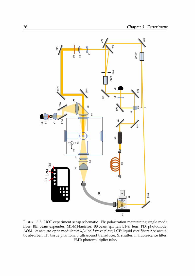
FIGURE 3.8: UOT experiment setup schematic. FB: polarization maintaining single modefiber; BE: beam expender; M1-M14:mirror; BS:beam splitter; L1-8: lens; PD: photodiode;AOM1-2: acousto-optic modulator; λ/2: half-wave plate; LCF: liquid core fiber; AA: acous-tic absorber; TP: tissue phantom; T:ultrasound transducer; S: shutter; F: fluorescence filter;
PMT: photomultiplier tube.
3.3. Ultrasound optical tomography 27
fill the cryostat inner window aperture. The pump beam polarization direction wasturned to D2 by a half-wave plate, then half of its power was cut down by a non-polarizing 50:50 beam splitter. The pump beam went through a linear polarizer P2(polarization direction: D2) before it entered the Pr (0.05%):YSO crystal inside thecryostat.
When the first AOM was off, most light (≈ 80%) went to the 0th order. The beamthen reached the second AOM (Isomet, 1205c-1). An iris was used to block the 0thorder of beam from the second AOM, the 1st order of beam (≈ 70%) sent directlyonto the tissue phantom, and the scattered light was collected by a liquid core fiber(Rofin, D = 10 mm, NA = 0.59). A plano-convex L4 (D = 72 mm, f = 52 mm, NA= 0.57) was used to collimate as much diffused light as possible. The collimatedbeam went through a linear polarizer P1 (only light with polarization direction D2
can pass through the polarizer) (colorPol VISIR, D = 50.8 mm) then refocused ontothe cryostat inner window with another plano-convex lens L5 (D = 50 mm, f = 150mm, NA = 0.16). Based on the COMSOL ray trace simulation, maximum 8% of thelight out of the LCF can be imaged onto the crystal aperture, see Appendix A.2. Thespectrally filtered light exiting from the crystal was also diffused light, half amountof the exited polarized light from the BS was then focused by a plano-convex lensL6 (D = 50 mm, f = 150 mm, NA = 0.16). Due to the aperture of the optical shutterS (Uniblitz VS14, D = 14 mm) was small, a pair of aspherical lenses L7 (D = 50 mm,f = 25 mm) and L8 (D = 50 mm, f = 45 mm) were used to focus the beam small onpassing through the shutter aperture. The beam was then refocused onto the photo-multiplier tube (Hamamatsu, R943-02) after it went through a 10 nm bandpass filter(Chroma HQ605/10).
The pumping and probing beam paths are counter-propagated to minimize the pos-sibility of accidentally exposing the full power pumping light onto the PMT. The op-tical shutter was kept closed during pumping and erasing mode, and then it openedfor 10 ms to receive the probe signal, afterward, it was closed again. Room light wasturned off during the UOT measurement. A black box was also built around PMT toblock background and scattered light in the room. The polarizer P2 was used to pu-rify the incoming pumping light polarization and prevent the unpolarized outgoingprobing light.
3.3.2 ProceduresFrom the US measurement, the US has a center frequency of 1.6 MHz and a band-width approximately 1 MHz. The prepared spectral filter has bandwidth 1 MHz tocover the US modulated sideband bandwidth. Some aquasonic US gel was appliedon the surface of the tissue phantom (air acoustic impedance, 430 kgm−2 s−1, is a lotdifferent to water, 1.48 ·106 kgm−2 s−1 [21]), the gel is used to fix the interface prob-lem so most US would transmit into the agar phantom instead of being reflected
28 Chapter 3. Experiment
back. The transducer X5-1 was placed in contact with the tissue phantom. If thetissue phantom height and length and width is smaller than 15 cm, the phantomoutline shape can be observed in the B mode scan (as echoes). The US scanner wasset to PW-mode with the smallest focus, the output trigger of US scanner was thentriggering the laser sequence.
Pulse sequence
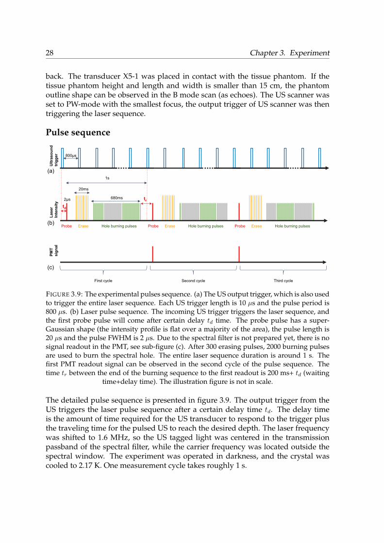
FIGURE 3.9: The experimental pulses sequence. (a) The US output trigger, which is also usedto trigger the entire laser sequence. Each US trigger length is 10 µs and the pulse period is800 µs. (b) Laser pulse sequence. The incoming US trigger triggers the laser sequence, andthe first probe pulse will come after certain delay td time. The probe pulse has a super-Gaussian shape (the intensity profile is flat over a majority of the area), the pulse length is20 µs and the pulse FWHM is 2 µs. Due to the spectral filter is not prepared yet, there is nosignal readout in the PMT, see sub-figure (c). After 300 erasing pulses, 2000 burning pulsesare used to burn the spectral hole. The entire laser sequence duration is around 1 s. Thefirst PMT readout signal can be observed in the second cycle of the pulse sequence. Thetime tr between the end of the burning sequence to the first readout is 200 ms+ td (waiting
time+delay time). The illustration figure is not in scale.
The detailed pulse sequence is presented in figure 3.9. The output trigger from theUS triggers the laser pulse sequence after a certain delay time td. The delay timeis the amount of time required for the US transducer to respond to the trigger plusthe traveling time for the pulsed US to reach the desired depth. The laser frequencywas shifted to 1.6 MHz, so the US tagged light was centered in the transmissionpassband of the spectral filter, while the carrier frequency was located outside thespectral window. The experiment was operated in darkness, and the crystal wascooled to 2.17 K. One measurement cycle takes roughly 1 s.
29
Chapter 4
Results and discussion
4.1 Tissue models
A direct approach of modeling tissue optical properties is by mixing absorber andscatterer with appropriate proportions, such that the tissue phantom optical param-eters can be predicted from the individual characteristics. Liquid phantoms allowquick and easy variation of the optical properties and free movement of the detectorwithin the medium, while solid phantom allows manufacturing macroscopic inho-mogeneous phantom to simulate biological tissue with complex structure.
4.1.1 Liquid phantom
Intralipid: scattering coefficient
(cm-1)
(cm-1)
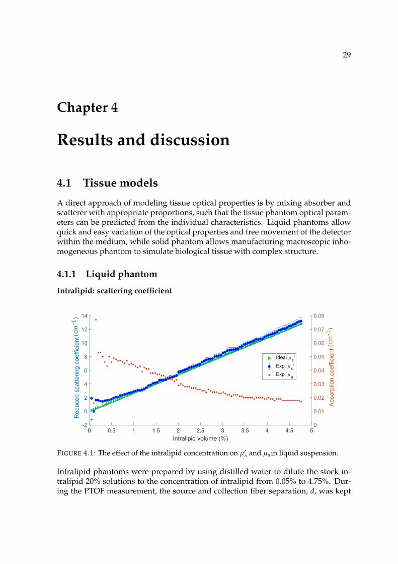
FIGURE 4.1: The effect of the intralipid concentration on µ′s and µain liquid suspension.
Intralipid phantoms were prepared by using distilled water to dilute the stock in-tralipid 20% solutions to the concentration of intralipid from 0.05% to 4.75%. Dur-ing the PTOF measurement, the source and collection fiber separation, d, was kept
30 Chapter 4. Results and discussion
constant (20 mm). The d value was also involved during the Monte Carlo fittingprogress. If the input d value is larger than the actual separation distance, the pho-tons are expected to travel a longer path, the time dispersion curve FWHM will bebroader, curve peak value drops and its position shifts to the later photons side,this would result the µ′s from the Monte Carlo fitting is larger than the actual value.Thus, for d± 0.5 mm, results in a roughly 5% uncertainty in the calculated µ′s.
The µ′s increases proportionately to intralipid concentration for both theoretical andexperimental data. The theoretical values were calculated by using equation 2.3at wavelength 606 nm. First few experimental data points for µ′s are offset fromthe curve trend, see figure 4.1. This is due to at low scattering coefficient, a largenumber of photons were reflected from the bottom of the liquid suspension, whichcauses a computational error for the time of flight. Ideally, intralipid should have noabsorption (absorption due to water, µa = 0.0026 cm−1 at 606 nm[16] ), but based onthe experimental measurement, the intralipid has 0.02 cm−1 absorption coefficient.From figure 4.1, it seems the absorption curve is slowly reaching a plateau withincreasing intralipid concentration. It is mostly due to the Monte Carlo fitting. Whenthe scattering is high, less reflected light from the container surface would affect thetime dispersion curve fitting result.
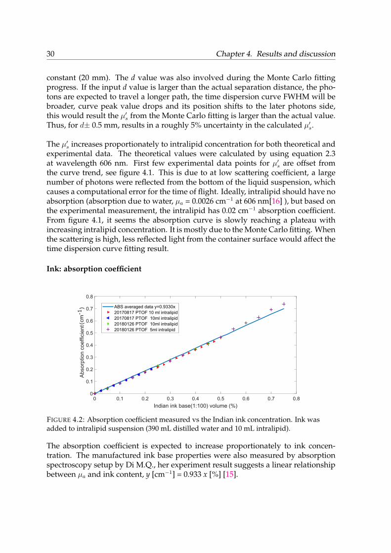
Ink: absorption coefficient
(cm-1)
FIGURE 4.2: Absorption coefficient measured vs the Indian ink concentration. Ink wasadded to intralipid suspension (390 mL distilled water and 10 mL intralipid).
The absorption coefficient is expected to increase proportionately to ink concen-tration. The manufactured ink base properties were also measured by absorptionspectroscopy setup by Di M.Q., her experiment result suggests a linear relationshipbetween µa and ink content, y [cm−1] = 0.933 x [%] [15].
4.1. Tissue models 31
For intralipid, the anisotropy of the scatterer suspension is independent of scattererconcentration. However, this does not apply to the ink sample case. First, intralipidparticles are on the scale of a nanometer while ink particles are on the scale of amicrometer. Increase large size particle concentration would increase the albedo ofthe liquid phantom. When the ink base concentration is lower than 0.5%, the trendof the curve is mostly linear, after 0.5% the gradient of curve increases. This couldbe due to the large size ink particle at high concentration is highly influencing theliquid phantom anisotropy, and the particles could be coalesced and formed largerparticles. Another possibility could be there were an insufficient number of photonsfor Monte Carlo to address an accurate data fitting, as the measurement had to stopat 0.75% since there was not enough signal.
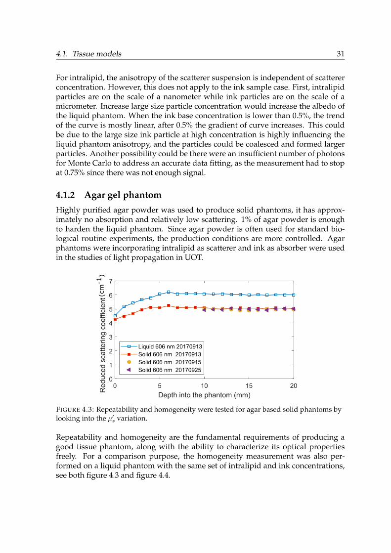
4.1.2 Agar gel phantomHighly purified agar powder was used to produce solid phantoms, it has approx-imately no absorption and relatively low scattering. 1% of agar powder is enoughto harden the liquid phantom. Since agar powder is often used for standard bio-logical routine experiments, the production conditions are more controlled. Agarphantoms were incorporating intralipid as scatterer and ink as absorber were usedin the studies of light propagation in UOT.
(cm-1)
FIGURE 4.3: Repeatability and homogeneity were tested for agar based solid phantoms bylooking into the µ′s variation.
Repeatability and homogeneity are the fundamental requirements of producing agood tissue phantom, along with the ability to characterize its optical propertiesfreely. For a comparison purpose, the homogeneity measurement was also per-formed on a liquid phantom with the same set of intralipid and ink concentrations,see both figure 4.3 and figure 4.4.
32 Chapter 4. Results and discussion
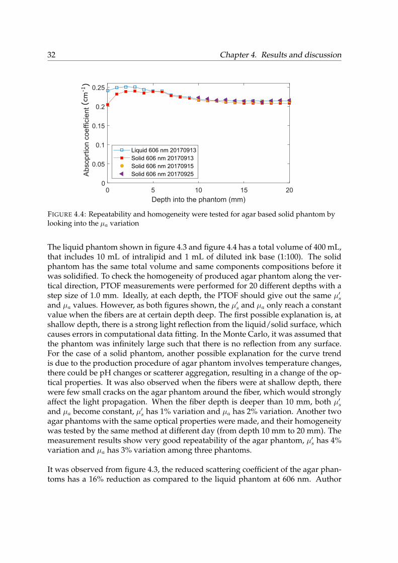
FIGURE 4.4: Repeatability and homogeneity were tested for agar based solid phantom bylooking into the µa variation
The liquid phantom shown in figure 4.3 and figure 4.4 has a total volume of 400 mL,that includes 10 mL of intralipid and 1 mL of diluted ink base (1:100). The solidphantom has the same total volume and same components compositions before itwas solidified. To check the homogeneity of produced agar phantom along the ver-tical direction, PTOF measurements were performed for 20 different depths with astep size of 1.0 mm. Ideally, at each depth, the PTOF should give out the same µ′sand µa values. However, as both figures shown, the µ′s and µa only reach a constantvalue when the fibers are at certain depth deep. The first possible explanation is, atshallow depth, there is a strong light reflection from the liquid/solid surface, whichcauses errors in computational data fitting. In the Monte Carlo, it was assumed thatthe phantom was infinitely large such that there is no reflection from any surface.For the case of a solid phantom, another possible explanation for the curve trendis due to the production procedure of agar phantom involves temperature changes,there could be pH changes or scatterer aggregation, resulting in a change of the op-tical properties. It was also observed when the fibers were at shallow depth, therewere few small cracks on the agar phantom around the fiber, which would stronglyaffect the light propagation. When the fiber depth is deeper than 10 mm, both µ′sand µa become constant, µ′s has 1% variation and µa has 2% variation. Another twoagar phantoms with the same optical properties were made, and their homogeneitywas tested by the same method at different day (from depth 10 mm to 20 mm). Themeasurement results show very good repeatability of the agar phantom, µ′s has 4%variation and µa has 3% variation among three phantoms.
It was observed from figure 4.3, the reduced scattering coefficient of the agar phan-toms has a 16% reduction as compared to the liquid phantom at 606 nm. Author
4.2. Ultrasound focus 33
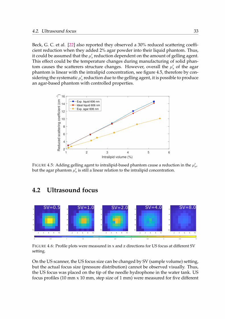
Beck, G. C. et al. [22] also reported they observed a 30% reduced scattering coeffi-cient reduction when they added 2% agar powder into their liquid phantom. Thus,it could be assumed that the µ′s reduction dependent on the amount of gelling agent.This effect could be the temperature changes during manufacturing of solid phan-tom causes the scatterers structure changes. However, overall the µ′s of the agarphantom is linear with the intralipid concentration, see figure 4.5, therefore by con-sidering the systematic µ′s reduction due to the gelling agent, it is possible to producean agar-based phantom with controlled properties.
1 2 3 4 5 6
Intralipid volume (%)
2
4
6
8
10
12
14
16
Reduced s
cattering c
oeffic
ient (c
m-1
)
Exp. liquid 606 nm
Ideal liquid 606 nm
Exp. agar 606 nm
FIGURE 4.5: Adding gelling agent to intralipid-based phantom cause a reduction in the µ′s,but the agar phantom µ′s is still a linear relation to the intralipid concentration.
4.2 Ultrasound focus
SV=0.5 SV=1.0 SV=2.0 SV=4.0 SV=8.0
FIGURE 4.6: Profile plots were measured in x and z directions for US focus at different SVsetting.
On the US scanner, the US focus size can be changed by SV (sample volume) setting,but the actual focus size (pressure distribution) cannot be observed visually. Thus,the US focus was placed on the tip of the needle hydrophone in the water tank. USfocus profiles (10 mm x 10 mm, step size of 1 mm) were measured for five different
34 Chapter 4. Results and discussion
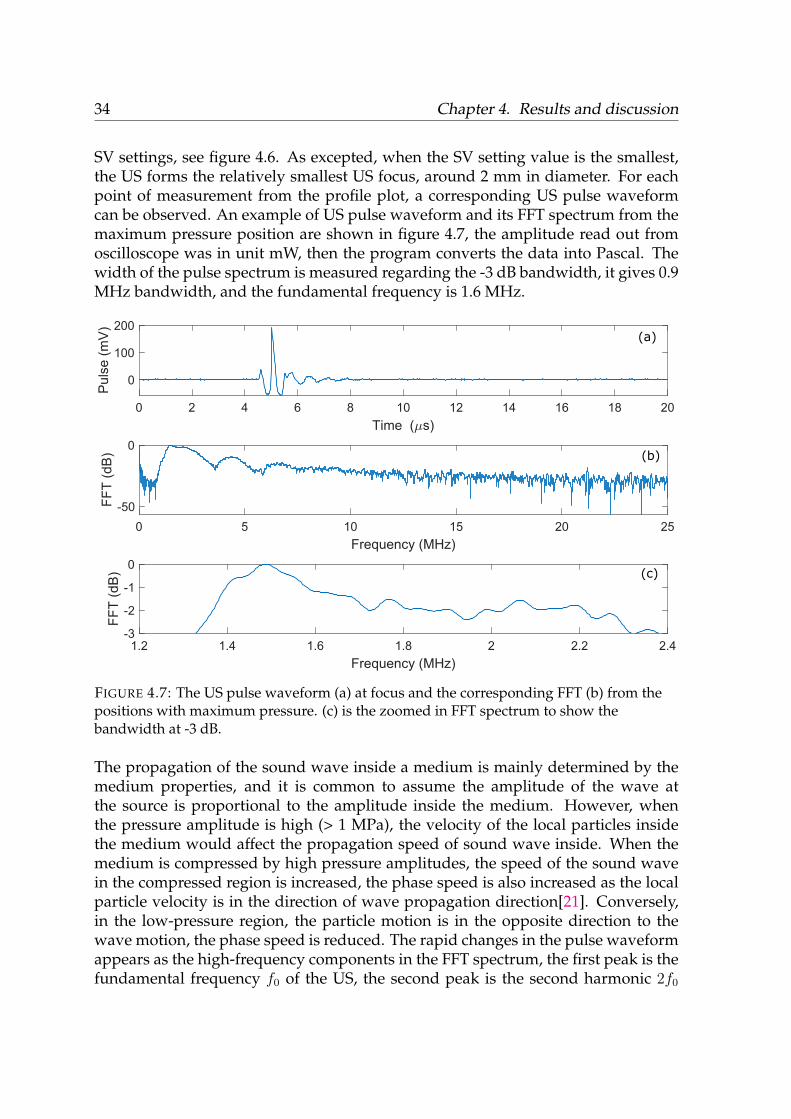
SV settings, see figure 4.6. As excepted, when the SV setting value is the smallest,the US forms the relatively smallest US focus, around 2 mm in diameter. For eachpoint of measurement from the profile plot, a corresponding US pulse waveformcan be observed. An example of US pulse waveform and its FFT spectrum from themaximum pressure position are shown in figure 4.7, the amplitude read out fromoscilloscope was in unit mW, then the program converts the data into Pascal. Thewidth of the pulse spectrum is measured regarding the -3 dB bandwidth, it gives 0.9MHz bandwidth, and the fundamental frequency is 1.6 MHz.
(a)
(b)
(c)
FIGURE 4.7: The US pulse waveform (a) at focus and the corresponding FFT (b) from thepositions with maximum pressure. (c) is the zoomed in FFT spectrum to show thebandwidth at -3 dB.
The propagation of the sound wave inside a medium is mainly determined by themedium properties, and it is common to assume the amplitude of the wave atthe source is proportional to the amplitude inside the medium. However, whenthe pressure amplitude is high (> 1 MPa), the velocity of the local particles insidethe medium would affect the propagation speed of sound wave inside. When themedium is compressed by high pressure amplitudes, the speed of the sound wavein the compressed region is increased, the phase speed is also increased as the localparticle velocity is in the direction of wave propagation direction[21]. Conversely,in the low-pressure region, the particle motion is in the opposite direction to thewave motion, the phase speed is reduced. The rapid changes in the pulse waveformappears as the high-frequency components in the FFT spectrum, the first peak is thefundamental frequency f0 of the US, the second peak is the second harmonic 2f0
4.2. Ultrasound focus 35
and the third peak is the third harmonics 3f0 and so on, see FFT spectrum in figure4.7. The higher the frequency is, the faster US pulse attenuates inside the medium,the power of the US also decreases as it propagates deeper, the pulse shape becomesrounded.
The US focus size determines the lateral resolution of UOT in the transverse direc-tion, the area with higher spatial amplitude distribution has about 2 mm diameterfor the smallest US focus setting (see figure 4.6). Thus, 2 mm is the minimum dis-tance that can be imaged for two objects that side to side and perpendicular to theUS propagation axis. The limitation of US focus is due to lack of access towards theoperating software. Otherwise, the smaller the US focus is in the transverse plane,the better the UOT can resolve small structure and close objects.
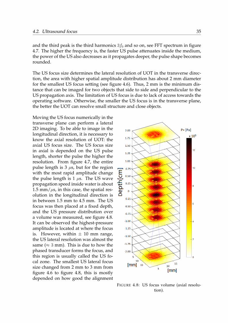
FIGURE 4.8: US focus volume (axial resolu-tion).
Moving the US focus numerically in thetransverse plane can perform a lateral2D imaging. To be able to image in thelongitudinal direction, it is necessary toknow the axial resolution of UOT: theaxial US focus size. The US focus sizein axial is depended on the US pulselength, shorter the pulse the higher theresolution. From figure 4.7, the entirepulse length is 3 µs, but for the regionwith the most rapid amplitude changethe pulse length is 1 µs. The US wavepropagation speed inside water is about1.5 mm/µs, in this case, the spatial res-olution in the longitudinal direction isin between 1.5 mm to 4.5 mm. The USfocus was then placed at a fixed depth,and the US pressure distribution overa volume was measured, see figure 4.8.It can be observed the highest-pressureamplitude is located at where the focusis. However, within ± 10 mm range,the US lateral resolution was almost thesame (≈ 3 mm). This is due to how thephased transducer forms the focus, andthis region is usually called the US fo-cal zone. The smallest US lateral focussize changed from 2 mm to 3 mm fromfigure 4.6 to figure 4.8, this is mostlydepended on how good the alignment
36 Chapter 4. Results and discussion
was, in figure 4.6 the highest-pressure point is not centered, it is possible the hy-drophone was not properly aligned with the US propagation axis. The lateral focussize is larger than the axial focus size, as the lateral focus is dependent on how goodthe transducer forms the focus while axial focus size is depended on the US pulselength.
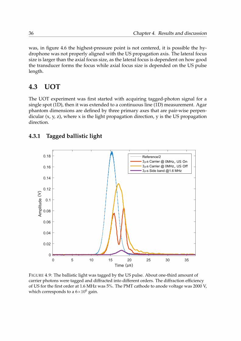
4.3 UOT
The UOT experiment was first started with acquiring tagged-photon signal for asingle spot (1D), then it was extended to a continuous line (1D) measurement. Agarphantom dimensions are defined by three primary axes that are pair-wise perpen-dicular (x, y, z), where x is the light propagation direction, y is the US propagationdirection.
4.3.1 Tagged ballistic light
FIGURE 4.9: The ballistic light was tagged by the US pulse. About one-third amount ofcarrier photons were tagged and diffracted into different orders. The diffraction efficiencyof US for the first order at 1.6 MHz was 5%. The PMT cathode to anode voltage was 2000 V,which corresponds to a 6×10⁶ gain.
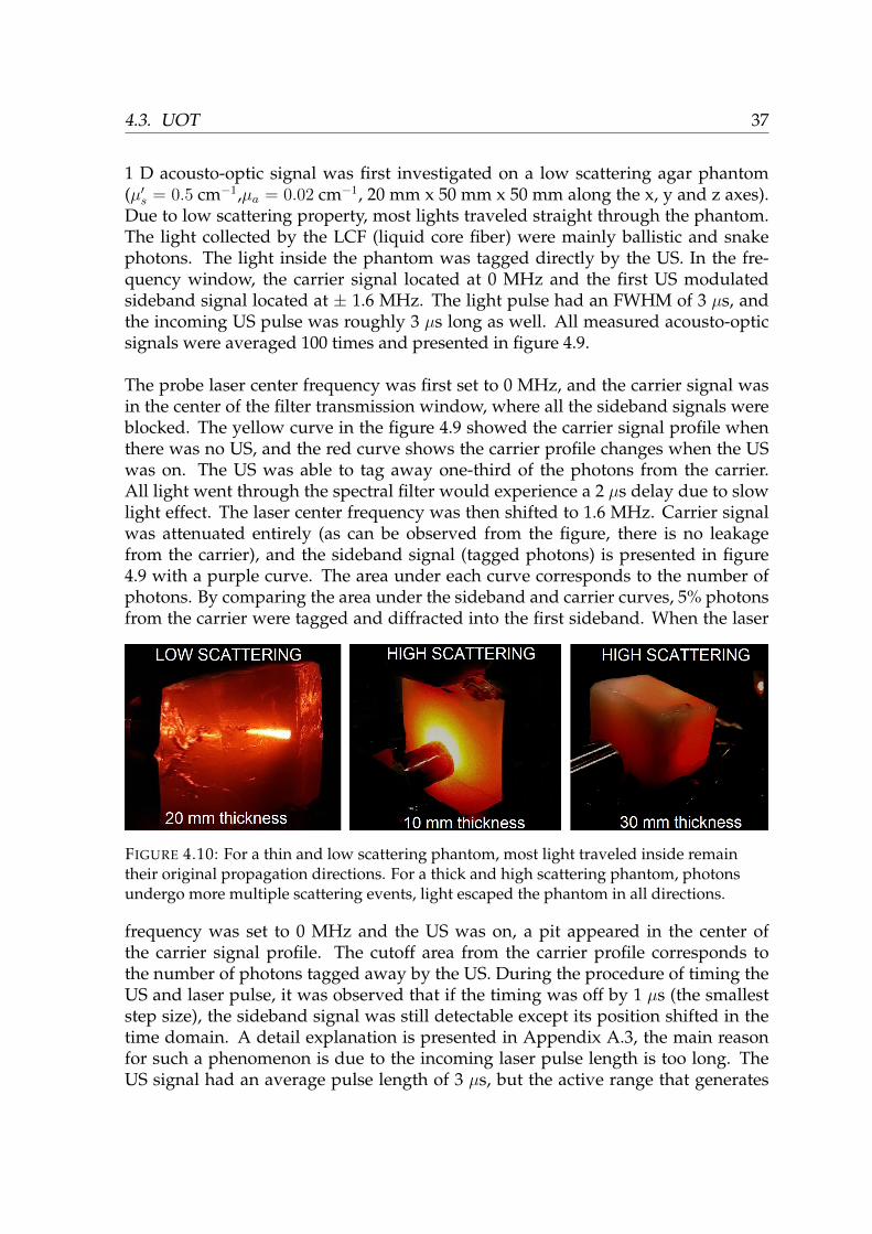
4.3. UOT 37
1 D acousto-optic signal was first investigated on a low scattering agar phantom(µ′s = 0.5 cm−1,µa = 0.02 cm−1, 20 mm x 50 mm x 50 mm along the x, y and z axes).Due to low scattering property, most lights traveled straight through the phantom.The light collected by the LCF (liquid core fiber) were mainly ballistic and snakephotons. The light inside the phantom was tagged directly by the US. In the fre-quency window, the carrier signal located at 0 MHz and the first US modulatedsideband signal located at ± 1.6 MHz. The light pulse had an FWHM of 3 µs, andthe incoming US pulse was roughly 3 µs long as well. All measured acousto-opticsignals were averaged 100 times and presented in figure 4.9.
The probe laser center frequency was first set to 0 MHz, and the carrier signal wasin the center of the filter transmission window, where all the sideband signals wereblocked. The yellow curve in the figure 4.9 showed the carrier signal profile whenthere was no US, and the red curve shows the carrier profile changes when the USwas on. The US was able to tag away one-third of the photons from the carrier.All light went through the spectral filter would experience a 2 µs delay due to slowlight effect. The laser center frequency was then shifted to 1.6 MHz. Carrier signalwas attenuated entirely (as can be observed from the figure, there is no leakagefrom the carrier), and the sideband signal (tagged photons) is presented in figure4.9 with a purple curve. The area under each curve corresponds to the number ofphotons. By comparing the area under the sideband and carrier curves, 5% photonsfrom the carrier were tagged and diffracted into the first sideband. When the laser
FIGURE 4.10: For a thin and low scattering phantom, most light traveled inside remaintheir original propagation directions. For a thick and high scattering phantom, photonsundergo more multiple scattering events, light escaped the phantom in all directions.
frequency was set to 0 MHz and the US was on, a pit appeared in the center ofthe carrier signal profile. The cutoff area from the carrier profile corresponds tothe number of photons tagged away by the US. During the procedure of timing theUS and laser pulse, it was observed that if the timing was off by 1 µs (the smalleststep size), the sideband signal was still detectable except its position shifted in thetime domain. A detail explanation is presented in Appendix A.3, the main reasonfor such a phenomenon is due to the incoming laser pulse length is too long. TheUS signal had an average pulse length of 3 µs, but the active range that generates
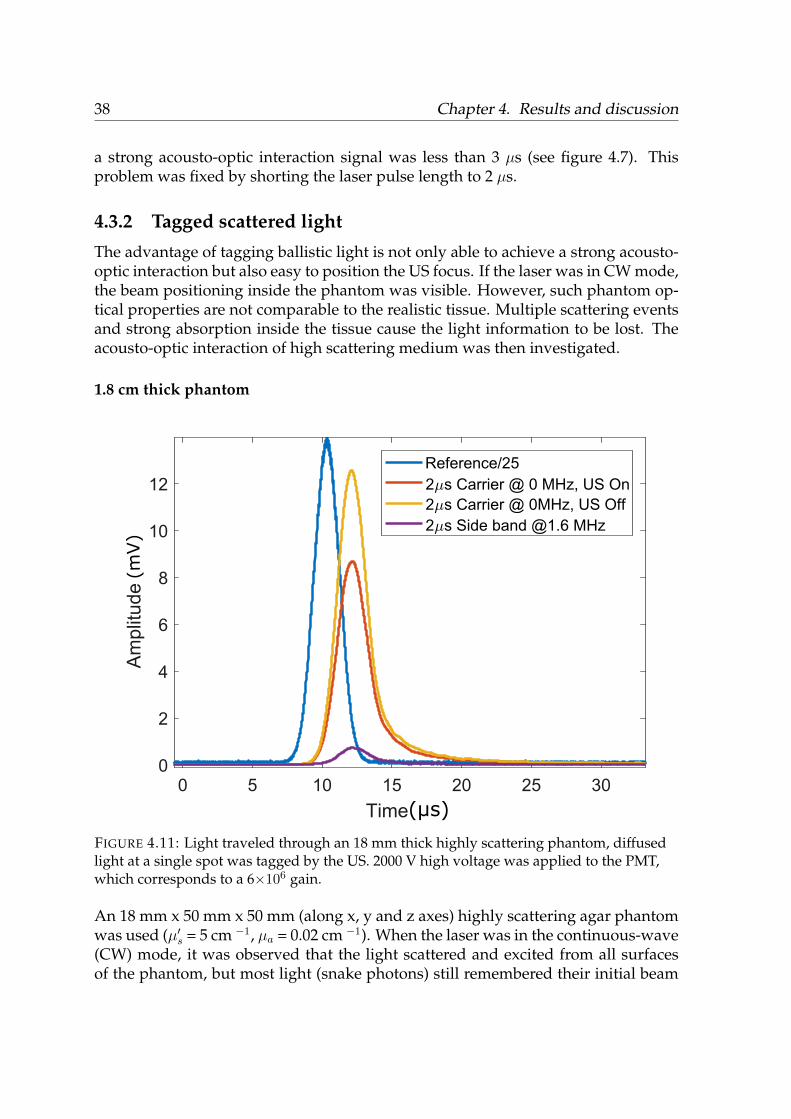
38 Chapter 4. Results and discussion
a strong acousto-optic interaction signal was less than 3 µs (see figure 4.7). Thisproblem was fixed by shorting the laser pulse length to 2 µs.
4.3.2 Tagged scattered lightThe advantage of tagging ballistic light is not only able to achieve a strong acousto-optic interaction but also easy to position the US focus. If the laser was in CW mode,the beam positioning inside the phantom was visible. However, such phantom op-tical properties are not comparable to the realistic tissue. Multiple scattering eventsand strong absorption inside the tissue cause the light information to be lost. Theacousto-optic interaction of high scattering medium was then investigated.
1.8 cm thick phantom
FIGURE 4.11: Light traveled through an 18 mm thick highly scattering phantom, diffusedlight at a single spot was tagged by the US. 2000 V high voltage was applied to the PMT,which corresponds to a 6×10⁶ gain.
An 18 mm x 50 mm x 50 mm (along x, y and z axes) highly scattering agar phantomwas used (µ′s = 5 cm −1, µa = 0.02 cm −1). When the laser was in the continuous-wave(CW) mode, it was observed that the light scattered and excited from all surfacesof the phantom, but most light (snake photons) still remembered their initial beam
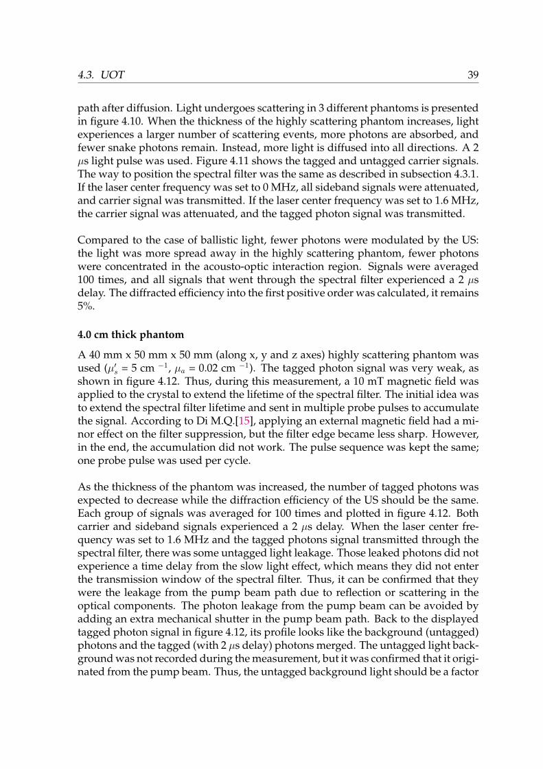
4.3. UOT 39
path after diffusion. Light undergoes scattering in 3 different phantoms is presentedin figure 4.10. When the thickness of the highly scattering phantom increases, lightexperiences a larger number of scattering events, more photons are absorbed, andfewer snake photons remain. Instead, more light is diffused into all directions. A 2µs light pulse was used. Figure 4.11 shows the tagged and untagged carrier signals.The way to position the spectral filter was the same as described in subsection 4.3.1.If the laser center frequency was set to 0 MHz, all sideband signals were attenuated,and carrier signal was transmitted. If the laser center frequency was set to 1.6 MHz,the carrier signal was attenuated, and the tagged photon signal was transmitted.
Compared to the case of ballistic light, fewer photons were modulated by the US:the light was more spread away in the highly scattering phantom, fewer photonswere concentrated in the acousto-optic interaction region. Signals were averaged100 times, and all signals that went through the spectral filter experienced a 2 µsdelay. The diffracted efficiency into the first positive order was calculated, it remains5%.
4.0 cm thick phantom
A 40 mm x 50 mm x 50 mm (along x, y and z axes) highly scattering phantom wasused (µ′s = 5 cm −1, µa = 0.02 cm −1). The tagged photon signal was very weak, asshown in figure 4.12. Thus, during this measurement, a 10 mT magnetic field wasapplied to the crystal to extend the lifetime of the spectral filter. The initial idea wasto extend the spectral filter lifetime and sent in multiple probe pulses to accumulatethe signal. According to Di M.Q.[15], applying an external magnetic field had a mi-nor effect on the filter suppression, but the filter edge became less sharp. However,in the end, the accumulation did not work. The pulse sequence was kept the same;one probe pulse was used per cycle.
As the thickness of the phantom was increased, the number of tagged photons wasexpected to decrease while the diffraction efficiency of the US should be the same.Each group of signals was averaged for 100 times and plotted in figure 4.12. Bothcarrier and sideband signals experienced a 2 µs delay. When the laser center fre-quency was set to 1.6 MHz and the tagged photons signal transmitted through thespectral filter, there was some untagged light leakage. Those leaked photons did notexperience a time delay from the slow light effect, which means they did not enterthe transmission window of the spectral filter. Thus, it can be confirmed that theywere the leakage from the pump beam path due to reflection or scattering in theoptical components. The photon leakage from the pump beam can be avoided byadding an extra mechanical shutter in the pump beam path. Back to the displayedtagged photon signal in figure 4.12, its profile looks like the background (untagged)photons and the tagged (with 2 µs delay) photons merged. The untagged light back-ground was not recorded during the measurement, but it was confirmed that it origi-nated from the pump beam. Thus, the untagged background light should be a factor
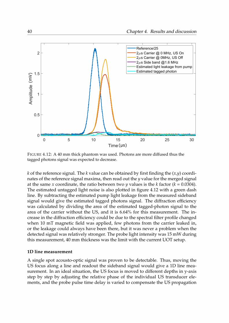
40 Chapter 4. Results and discussion(mV)
(µs)
FIGURE 4.12: A 40 mm thick phantom was used. Photons are more diffused thus thetagged photons signal was expected to decrease.
k of the reference signal. The k value can be obtained by first finding the (x,y) coordi-nates of the reference signal maxima, then read out the y value for the merged signalat the same x coordinate, the ratio between two y values is the k factor (k = 0.0304).The estimated untagged light noise is also plotted in figure 4.12 with a green dashline. By subtracting the estimated pump light leakage from the measured sidebandsignal would give the estimated tagged photons signal. The diffraction efficiencywas calculated by dividing the area of the estimated tagged-photon signal to thearea of the carrier without the US, and it is 6.64% for this measurement. The in-crease in the diffraction efficiency could be due to the spectral filter profile changedwhen 10 mT magnetic field was applied, few photons from the carrier leaked in,or the leakage could always have been there, but it was never a problem when thedetected signal was relatively stronger. The probe light intensity was 15 mW duringthis measurement, 40 mm thickness was the limit with the current UOT setup.
1D line measurement
A single spot acousto-optic signal was proven to be detectable. Thus, moving theUS focus along a line and readout the sideband signal would give a 1D line mea-surement. In an ideal situation, the US focus is moved to different depths in y-axisstep by step by adjusting the relative phase of the individual US transducer ele-ments, and the probe pulse time delay is varied to compensate the US propagation
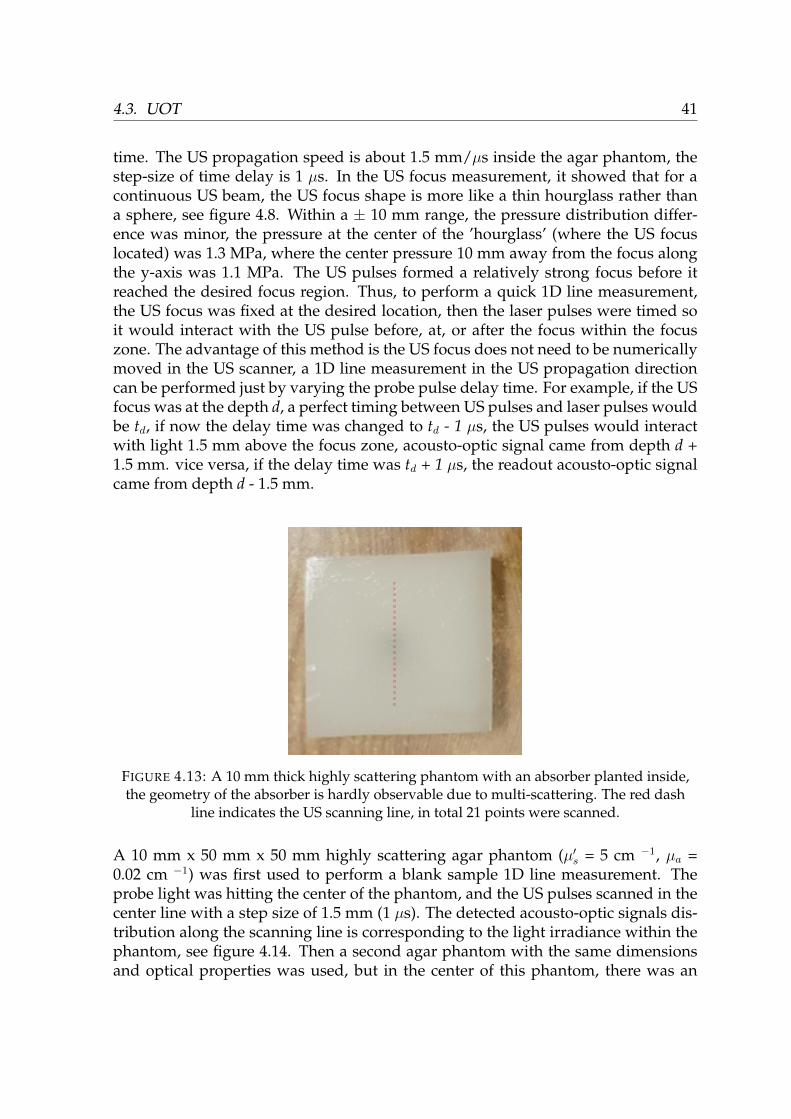
4.3. UOT 41
time. The US propagation speed is about 1.5 mm/µs inside the agar phantom, thestep-size of time delay is 1 µs. In the US focus measurement, it showed that for acontinuous US beam, the US focus shape is more like a thin hourglass rather thana sphere, see figure 4.8. Within a ± 10 mm range, the pressure distribution differ-ence was minor, the pressure at the center of the ’hourglass’ (where the US focuslocated) was 1.3 MPa, where the center pressure 10 mm away from the focus alongthe y-axis was 1.1 MPa. The US pulses formed a relatively strong focus before itreached the desired focus region. Thus, to perform a quick 1D line measurement,the US focus was fixed at the desired location, then the laser pulses were timed soit would interact with the US pulse before, at, or after the focus within the focuszone. The advantage of this method is the US focus does not need to be numericallymoved in the US scanner, a 1D line measurement in the US propagation directioncan be performed just by varying the probe pulse delay time. For example, if the USfocus was at the depth d, a perfect timing between US pulses and laser pulses wouldbe td, if now the delay time was changed to td - 1 µs, the US pulses would interactwith light 1.5 mm above the focus zone, acousto-optic signal came from depth d +1.5 mm. vice versa, if the delay time was td + 1 µs, the readout acousto-optic signalcame from depth d - 1.5 mm.
FIGURE 4.13: A 10 mm thick highly scattering phantom with an absorber planted inside,the geometry of the absorber is hardly observable due to multi-scattering. The red dash
line indicates the US scanning line, in total 21 points were scanned.
A 10 mm x 50 mm x 50 mm highly scattering agar phantom (µ′s = 5 cm −1, µa =0.02 cm −1) was first used to perform a blank sample 1D line measurement. Theprobe light was hitting the center of the phantom, and the US pulses scanned in thecenter line with a step size of 1.5 mm (1 µs). The detected acousto-optic signals dis-tribution along the scanning line is corresponding to the light irradiance within thephantom, see figure 4.14. Then a second agar phantom with the same dimensionsand optical properties was used, but in the center of this phantom, there was an
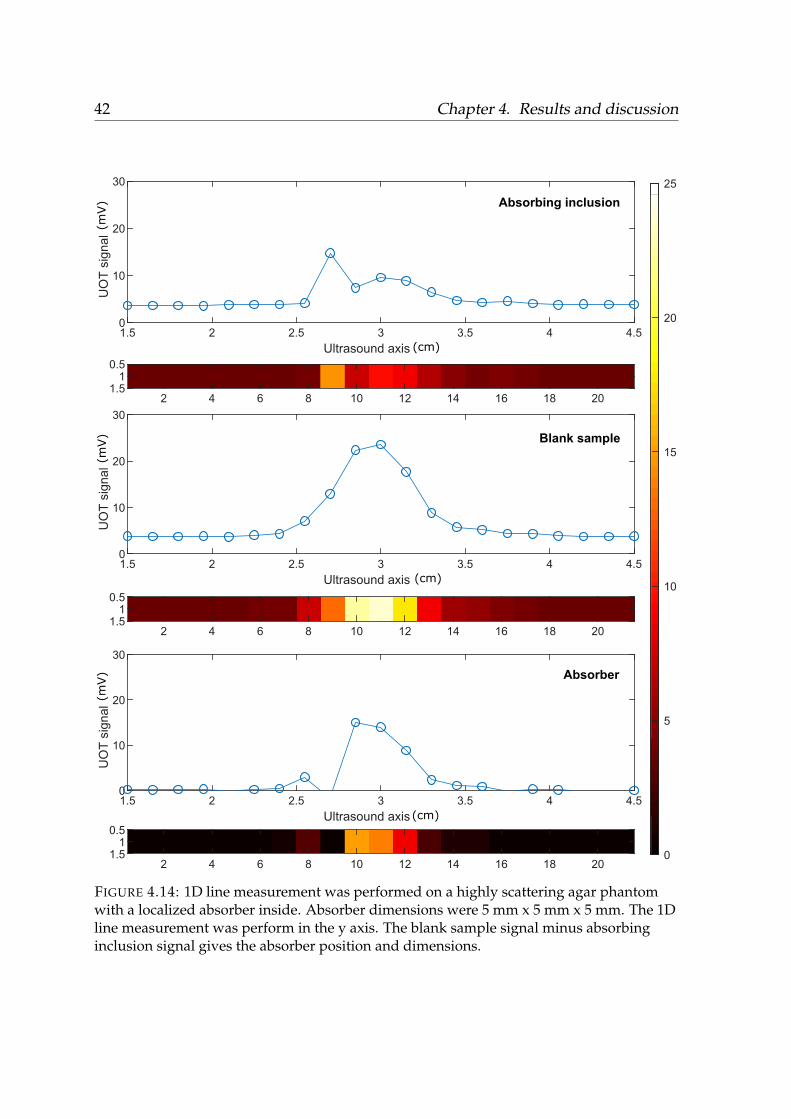
42 Chapter 4. Results and discussion(mV)
(cm)
(cm)
(cm)
(mV)
(mV)
FIGURE 4.14: 1D line measurement was performed on a highly scattering agar phantomwith a localized absorber inside. Absorber dimensions were 5 mm x 5 mm x 5 mm. The 1Dline measurement was perform in the y axis. The blank sample signal minus absorbinginclusion signal gives the absorber position and dimensions.
4.3. UOT 43
absorber implanted. The size of the absorber was 5 mm x 5 mm x 5 mm. A photoof the phantom with the absorbing inclusion is shown in figure 4.13. The reasonfor choosing this size of absorber was, the current UOT resolution was around 2 -3 mm, if the absorber was too small, it may not be observed in the line scanning; ifthe absorber was too big, it would absorb a large proportion of light scattered insidethe medium, it will lower the acousto-optic signal strength when there was alreadyvery low amount of probe light. The reason for choosing a thin slice of scatteringphantom was, the goal was to perform deep tissue imaging with UOT, but before itwas possible to move forward towards a higher depth, it was necessary to prove thesystem was able to perform tissue imaging based on the acousto-optic signals. Witha 10 mm thickness, the localization of the absorber in the highly scattering phantomcan be observed by eyes. Thus, the UOT imaged result can be used to compare withthe visual observation.
The 1D line measurement result of absorbing inclusion phantom is presented infigure 4.14, the probe light was hitting the center of the phantom (also hitting theabsorber), US pulses scanned in the center line of the phantom. By subtracting theblank sample and absorber inclusion sample signals, it gives the absorber signaldistribution in the 1D line. The absorber dimension according to the UOT signalwas roughly 4*1.5 mm, that was 6 mm while the real size was 5 mm. Thus, thecurrent UOT setup can perform interior scanning of a highly scattering mediumbased on the acousto-optic signals, but its resolution is highly limited by the USfocus size, and the penetration depth is limited by the probe light power.
44
Chapter 5
Conclusion and Outlook
5.1 Conclusion
In summary, this thesis work encompassed manufacture tissue models with con-trolled optical properties and homogeneity, study the ultrasound property and de-velopment of ultrasound optical tomography (UOT) system. Strong absorption andscattering properties of the tissue are the primary factors that were limiting theoptically-based imaging system development. Use a wavelength from the opticalwindow with low tissue absorption would increase the light penetration depth, butit cannot fix the optical information loss due to multi-scattering events. The princi-ple of UOT is to tag the photons in the region of interest with ultrasound and thenfilter the tagged photons with a high finesse spectral filter. The UOT system wasvery sensitive to laser intensity and stability. When there was only 30 nJ (15 mW×2µs) probe light, the current UOT system can detect acousto-optic interaction signalfor a 40 mm thick highly scattering phantom, and it was able to perform a 1D linemeasurement for a highly scattering phantom (µ′s = 5 cm−1) with an inclusion inthe center, the inclusion dimension can be estimated from the 1D line measurement.The laser safety level is 20 mJ/cm 2 for pulsed light [23]. Thus, the laser energyused in this thesis work has an improvement factor of ≈ 106. Although the relationbetween the penetration depth in a highly scattering medium and the laser poweris nonlinear, increasing the probe laser power would still improve the penetrationdepth and contrast-to-noise ratio.
5.2 Outlook
Lack of control of the ultrasound scanner and low probing laser light power are thetwo main deficiencies of the current UOT system. The signal strength of UOT isdependent on the light irradiance inside the tissue and the focus size of the ultra-sound. In the current system, the UOT spatial resolution is 2 to 3 mm, which is farfrom the goal of resolving tissue structural properties in µm scale. The resolutionof UOT can be improved by using a smaller ultrasound focus, but that does notnecessarily mean that the UOT signal would be improved. A smaller ultrasoundvolume would modulate less number of photons, and the sideband signal might be
5.2. Outlook 45
so weak that cannot be distinguished from the detector dark noise. More photonscan be tagged if the ultrasound has a better diffraction efficiency. The diffractionefficiency of ultrasound can theoretically be improved by increasing the ultrasoundpressure level. Overall, the key to enhance UOT system performance is to find theoptimal balance between the UOT resolution and signal strength and deliver morephotons into the deep tissue and efficiently extract the weak tagged photons signalfrom the background. Tm:Y3Al5O12 (Tm +3:YAG) crystal has a transition at 793 nm,this wavelength is within the optical window, and it can be used to burn a persistentspectral hole at 1.8 K and last for more than 30 s [24]. This crystal could be a goodchoice for future developing a UOT system for clinical applications
There are a range of different improvements that can be addressed to the currentUOT setup. Since the lifetime of the spectral filter can be extended by applying anexternal magnetic field, send in multiple probe pulses and accumulate the signalswould speed up the UOT data acquiring time (instead of sending one probe pulseper cycle and wait for 100 s for a 100 times data averaging, 100 probe pulses canbe sent in one cycle and the averaged data would give the same result). The lasersafety level for pulse light was beam size dependent, expanding the probing beamto a bigger size would allow a higher power probe light, bigger volume of tissuewould be illuminated.
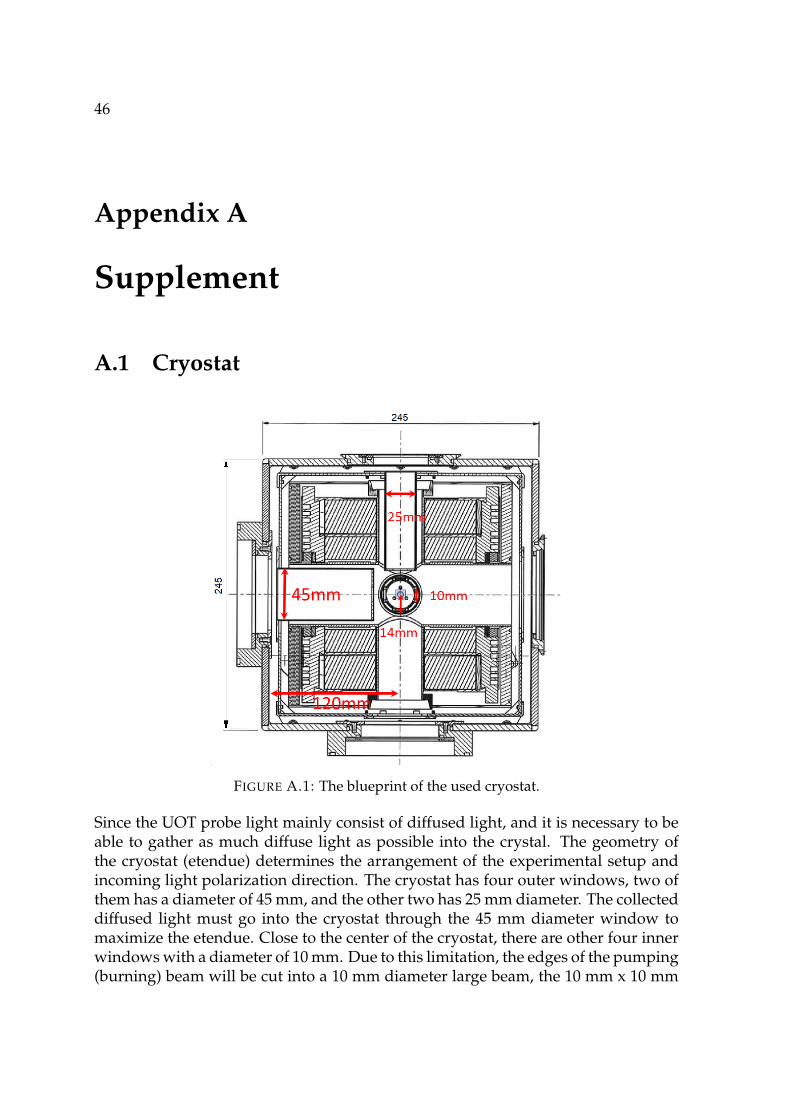
46
Appendix A
Supplement
A.1 Cryostat
FIGURE A.1: The blueprint of the used cryostat.
Since the UOT probe light mainly consist of diffused light, and it is necessary to beable to gather as much diffuse light as possible into the crystal. The geometry ofthe cryostat (etendue) determines the arrangement of the experimental setup andincoming light polarization direction. The cryostat has four outer windows, two ofthem has a diameter of 45 mm, and the other two has 25 mm diameter. The collecteddiffused light must go into the cryostat through the 45 mm diameter window tomaximize the etendue. Close to the center of the cryostat, there are other four innerwindows with a diameter of 10 mm. Due to this limitation, the edges of the pumping(burning) beam will be cut into a 10 mm diameter large beam, the 10 mm x 10 mm
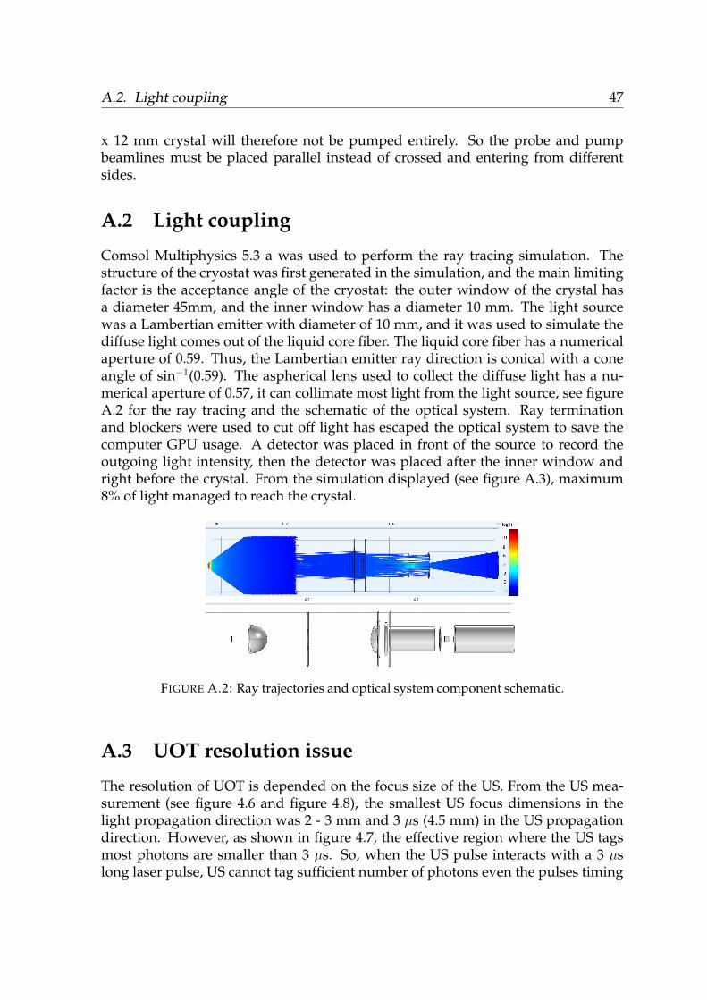
A.2. Light coupling 47
x 12 mm crystal will therefore not be pumped entirely. So the probe and pumpbeamlines must be placed parallel instead of crossed and entering from differentsides.
A.2 Light coupling
Comsol Multiphysics 5.3 a was used to perform the ray tracing simulation. Thestructure of the cryostat was first generated in the simulation, and the main limitingfactor is the acceptance angle of the cryostat: the outer window of the crystal hasa diameter 45mm, and the inner window has a diameter 10 mm. The light sourcewas a Lambertian emitter with diameter of 10 mm, and it was used to simulate thediffuse light comes out of the liquid core fiber. The liquid core fiber has a numericalaperture of 0.59. Thus, the Lambertian emitter ray direction is conical with a coneangle of sin−1(0.59). The aspherical lens used to collect the diffuse light has a nu-merical aperture of 0.57, it can collimate most light from the light source, see figureA.2 for the ray tracing and the schematic of the optical system. Ray terminationand blockers were used to cut off light has escaped the optical system to save thecomputer GPU usage. A detector was placed in front of the source to record theoutgoing light intensity, then the detector was placed after the inner window andright before the crystal. From the simulation displayed (see figure A.3), maximum8% of light managed to reach the crystal.
FIGURE A.2: Ray trajectories and optical system component schematic.
A.3 UOT resolution issue
The resolution of UOT is depended on the focus size of the US. From the US mea-surement (see figure 4.6 and figure 4.8), the smallest US focus dimensions in thelight propagation direction was 2 - 3 mm and 3 µs (4.5 mm) in the US propagationdirection. However, as shown in figure 4.7, the effective region where the US tagsmost photons are smaller than 3 µs. So, when the US pulse interacts with a 3 µslong laser pulse, US cannot tag sufficient number of photons even the pulses timing
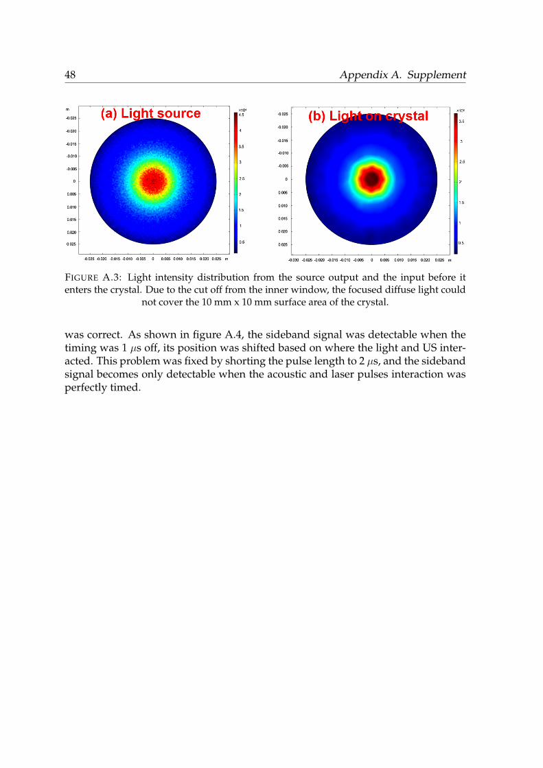
48 Appendix A. Supplement
FIGURE A.3: Light intensity distribution from the source output and the input before itenters the crystal. Due to the cut off from the inner window, the focused diffuse light could
not cover the 10 mm x 10 mm surface area of the crystal.
was correct. As shown in figure A.4, the sideband signal was detectable when thetiming was 1 µs off, its position was shifted based on where the light and US inter-acted. This problem was fixed by shorting the pulse length to 2 µs, and the sidebandsignal becomes only detectable when the acoustic and laser pulses interaction wasperfectly timed.
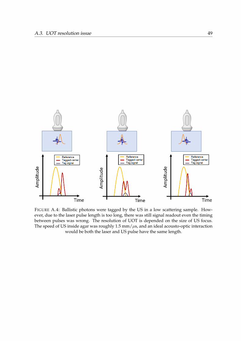
A.3. UOT resolution issue 49
FIGURE A.4: Ballistic photons were tagged by the US in a low scattering sample. How-ever, due to the laser pulse length is too long, there was still signal readout even the timingbetween pulses was wrong. The resolution of UOT is depended on the size of US focus.The speed of US inside agar was roughly 1.5 mm/µs, and an ideal acousto-optic interaction
would be both the laser and US pulse have the same length.
50
Bibliography
[1] H. Liu, “Advancing Upconversion Emissions for Biomedical Imaging”, PhDthesis, LRAP-484, Department of Atomic Physics, Lund University, 2014.
[2] J. M. Menter, “Temperature dependence of collagen fluorescence”, eng, Photo-chemical & Photobiological Sciences: Official Journal of the European PhotochemistryAssociation and the European Society for Photobiology, vol. 5, no. 4, pp. 403–410,Apr. 2006.
[3] A. Walther, L. Rippe, L. V. Wang, S. Andersson-Engels, and S. Kröll, “Analysisof the potential for non-invasive imaging of oxygenation at heart depth, usingultrasound optical tomography (UOT) or photo-acoustic tomography (PAT)”,EN, Biomedical Optics Express, vol. 8, no. 10, pp. 4523–4536, Oct. 2017.
[4] T. Valery, “Light scattering study of tissues”, vol. 40, p. 495, Oct. 2007.
[5] T. Valery, “Tissue optics and photonics: Light-tissue interaction”, Journal ofBiomedical Photonics & Engineering, vol. 1, no. 2, 2015.
[6] P. Di Ninni, F. Martelli, and G. Zaccanti, “Intralipid: Towards a diffusive ref-erence standard for optical”, vol. 56, N21–8, Jan. 2011.
[7] R. Michels, F. Foschum, and A. Kienle, “Optical properties of fat emulsions”,Opt. Express, vol. 16, no. 8, pp. 5907–5925, Apr. 2008.
[8] M. J. C. V. Gemert, S. L. Jacques, H. J. C. M. Sterenborg, and W. M. Star, “Skinoptics”, IEEE Transactions on Biomedical Engineering, vol. 36, no. 12, pp. 1146–1154, Dec. 1989.
[9] C. Boudoux, Fundamentals of biomedical optics: From light interactions with cellsto complex imaging systems. Pollux, 2017.
[10] E. Alerstam, S. Andersson-Engels, and T. Svensson, “White monte carlo fortime-resolved photon migration”, Journal of Biomedical Optics, vol. 13, 2008.
[11] A. Kienle and M. S. Patterson, “Determination of the optical properties of tur-bid media from a single monte carlo simulation”, Physics in Medicine and Biol-ogy, vol. 41, no. 10, p. 2221, 1996.
[12] E. Alerstam, S. Andersson-Engels, and T. Svensson, “Parallel computing withgraphics processing units for high-speed monte carlo simulation of photonmigration”, Journal of Biomedical Optics, vol. 13, 2008.
[13] E. Alerstam, S. Andersson-Engels, and T. Svensson, “Improved accuracy intime-resolved diffuse reflectance spectroscopy”, Opt. Express, vol. 16, no. 14,Jul. 2008.
BIBLIOGRAPHY 51
[14] W. Lihong V., “Mechanisms of ultrasonic modulation of multiply scatteredcoherent light: An analytic model”, Phys. Rev. Lett., vol. 87, p. 043 903, 4 Jul.2001.
[15] M. Q. Di, “Preparation of materials for deep tissue imaging with slow light”,MSc thesis, LRAP-545, Department of Atomic Physics, Lund University, 2018.
[16] V. M. Zolotarev, B. A. Mikhilov, L. L. Alperovich, and S. I. Popov, “Disper-sion and absorption of liquid water in the infrared and radio regions of thespectrum”, Optics and Spectroscopy, vol. 27, pp. 430–432, 1969.
[17] I. Driver, J. W. Feather, P. R. King, and J. B. Dawson, “The optical propertiesof aqueous suspensions of intralipid, a fat emulsion”, Physics in Medicine &Biology, vol. 34, no. 12, p. 1927, 1989.
[18] K. Pal, A. K. Banthia, and D. K. Majumdar, “Polymeric hydrogels: Characteri-zation and biomedical applications”, Designed Monomers and Polymers, vol. 12,no. 3, pp. 197–220, 2009.
[19] R. Cubeddu, A. Pifferi, P. Taroni, A. Torricelli, and G. Valentini, “A solid tissuephantom for photon migration studies”, Physics in Medicine & Biology, vol. 42,no. 10, p. 1971, 1997.
[20] B. Julsgaard, A. Walther, S. Kröll, and L. Rippe, “Understanding laser stabi-lization using spectral hole burning”, Opt. Express, vol. 15, no. 18, pp. 11 444–11 465, Sep. 2007.
[21] A. T. Peter R. Hoskins Kevin Martin, Diagnostic ultrasound: Physics and equip-ment. Cambridge University Press, 2010.
[22] G. C. Beck, N. Akgün, A. Rück, and R. Steiner, “Design and Characterisationof a Tissue Phantom System for Optical Diagnostics”, Lasers in Medical Science,vol. 13, pp. 160–171, Oct. 1998.
[23] American national standard for the safe use of lasers, standard z136.1- 2000 (ansi,inc., new york, 2000).
[24] N. Ohlsson, M. Nilsson, S. Kröll, and R. K. Mohan, “Long-time-storage mech-anism for tm:yag in a magnetic field”, Opt. Lett., vol. 28, no. 6, pp. 450–452,Mar. 2003.