Embed Size (px)
Citation preview
A Technique for Combining
Equalization with Differential Detection
Kenneth Mark Aleong, B.Eng.
Department of Electrical Engineering
McGill University, Montreal
June, 1991
A Thesis submitted to the Faculty of Graduate Studies and Research
in partial fulfillment of the requirements for the degree of Master of Engineering
@Kenneth Mark Aleong, 1991
Abstract
A technique for combining equalization and differentially coherent detection is pro-
posed for use in wireless communication when carrier phase recovery is difficult. A
decision-feedback differentially coherent scheme, which generates an improved refer-
ence phase, is combined with a linear equalizer and the LMS algorithm is used to
adapt the equalizer to an unknown channel. In addition, the proposed receiver is
simulated for various two-dimensional signal constellations over multipath channels.
It is shown that for high SNR, the degradation of this structure is negligible with
respect to combined coherent detection and equalization. Therefore, this equalized
differentially coherent detection scheme can be used when carrier phase tracking (i.e.
coherent detection) is difficult and intersymbol interference is a major obstacle.
Cette thke propose une technique combinant 1'6galisation et la dktection cohQente
diffirentielle pour la radiocommunication quand le rktablissement de la phase du
signal porteur est difficile. Un systkme cohdrent diffirentiel rktroaction amdiorant
la phase de rkfkrence est combini B un dgalisateur linthire. La prockdure "CMM" est
ensuite utilisk pour adapter l'kgalisateur B un canal inconnu. De plus, une simulation
du rkcepteur est faite avec des constellations de signaux B deux-dimensions pour des
canaux multi-routes. I1 est dkmontrk que, pour un grand RSB, la ddgradation de la
performance de cette technique est nkgligeable par rapport B la combination classique
de la dktection cohdrente et de l'kgalisation. Donc, cette technique de dktection
cohkrente diffkrentielle Cgalisk peut-&re utilisCe quand la poursuite de la phase du
signal porteur (c.a.d. la dktection cohkrente) est difficile et que l'interfhence entre
symboles est une probleme majeur.
Acknowledgement
I would sincerely like to thank Dr. Harry Leib for his numerous suggestions,
helpful advice, encouragement, understanding and perseverance in the realization of
this work.
I would also like to thank Dr. Peter Kabal for his invaluable guidance, un-
derstanding and financial support without which this work would not be done.
I wish to extend my gratitude to my loving parents and family for their
continuous support and encouragement throughout my studies.
I would like to thank all my friends for their support. Special thanks to
Aloknath De for his comments and to Marcel Sankeralli and Ronnie Quesnel for
translating the abstract into French.
I wish to thank the Information and Network Systems Laboratory especially
Sam Torrente and Ronnie Quesnel for their help with the computer simulations.
Contents
Abstract
Acknowledgement
Contents
List of Figures
List of Tables
List of Symbols
vii
viii
1 Introduction
2 Combining Equalization and Decision-Feedback Differentially Co-
herent Detection 4
2.1 Equalization and Decision-Feedback Differential Coherent Detection . 5
. . . . . . . . . . . . . . . . . . . . . . . . . 2.2 Baseband System Model 12
. . . . . . . . . . . . . . . . . . . . . . . . . . . . 2.2.1 Transmitter 12
. . . . . . . . . . . . . . . . . . . . . . . . . . . . . . 2.2.2 Channel 16
2.2.3 Receiver . . . . . . . . . . . . . . . . . . . . . . . . . . . . . . 17
. . . . . . . . 2.3 Comparison with Equalization and Coherent Detection 21
3 Equalization for Known Channels 23
. . . . . . . . . . . . . . . . . . . . . . . . . . . . . . 3.1 MMSE Analysis 23
. . . . . . . . . . . . . . . . . . 3.2 MMSE with Perfect Reference Phase 25
. . . . . . . . . . . . . . . . . . . . . 3.3 Reference Phase Error Analysis 29
. . . . . . . . . . . . . . . . . . . . . . . . . . . . . 3.4 Numerical Results 33
. . . . . . . . . . . . . . . . . . . . . . . . . . . . . . . . . 3.5 Observations 40
4 Adaptive Equalization for Unknown Channels 44
. . . . . . . . . . . . . . . . . . . . . . 4.1 The LMS Adaptive Equalizer 44
. . . . . . . . . . . . . . . . . . . . . . . . . . . . 4.2 Simulation Results 49
. . . . . . . . . . . . . . . . . . . . . . . . . . . . . . . . 4.3 Observations 60
5 Conclusions 63
. . . . . . . . . . . . . . . . . . . . . . 5.1 Suggestions for Further Work 65
Bibliography 66
Appendix A 70
. . . . . . . . . . . . . . . . . . . . . . . . . . . . A.l Program Overview 70
. . . . . . . . . . . . . . . . . . . A.2 MMSE Program File and Test Case 72
Appendix B 78
. . . . . . . . . . . . . . . . . . . B.l AMSE Program File and Test Case 76
. . . . . . . . . . . . . . . . . . . . . . . . . B.2 Additional Program Files 89
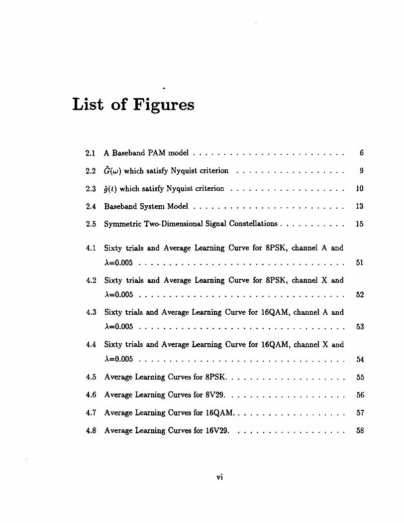
List of Figures
2.1 A Baseband PAM model . . . . . . . . . . . . . . . . . . . . . . . . . 6
. . . . . . . . . . . . . . . . . . 2.2 ~ ( w ) which satisfy Nyquist criterion 9
2.3 i j ( t ) which satisfy Nyquist criterion . . . . . . . . . . . . . . . . . . . 10
2.4 Baseband System Model . . . . . . . . . . . . . . . . . . . . . . . . . 13
2.5 Symmetric Two-Dimensional Signal Constellations . . . . . . . . . . . 15
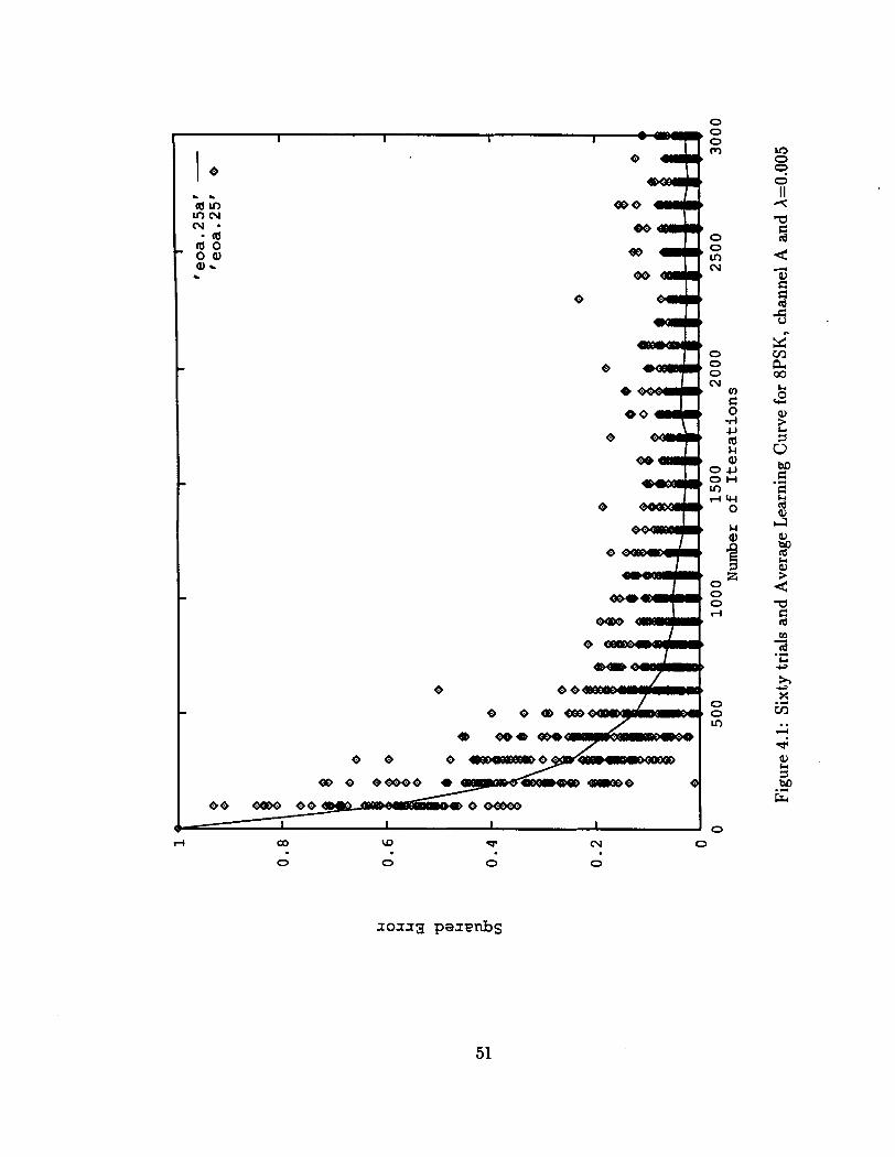
4.1 Sixty trials and Average Learning Curve for 8PSK. channel A and
A=0.005 . . . . . . . . . . . . . . . . . . . . . . . . . . . . . . . . . . 51
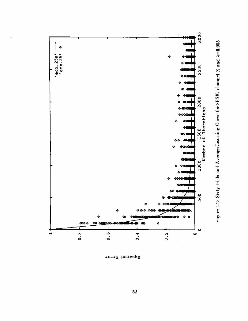
4.2 Sixty trials and Average Learning Curve for 8PSK. channel X and
A=0.005 . . . . . . . . . . . . . . . . . . . . . . . . . . . . . . . . . . 52
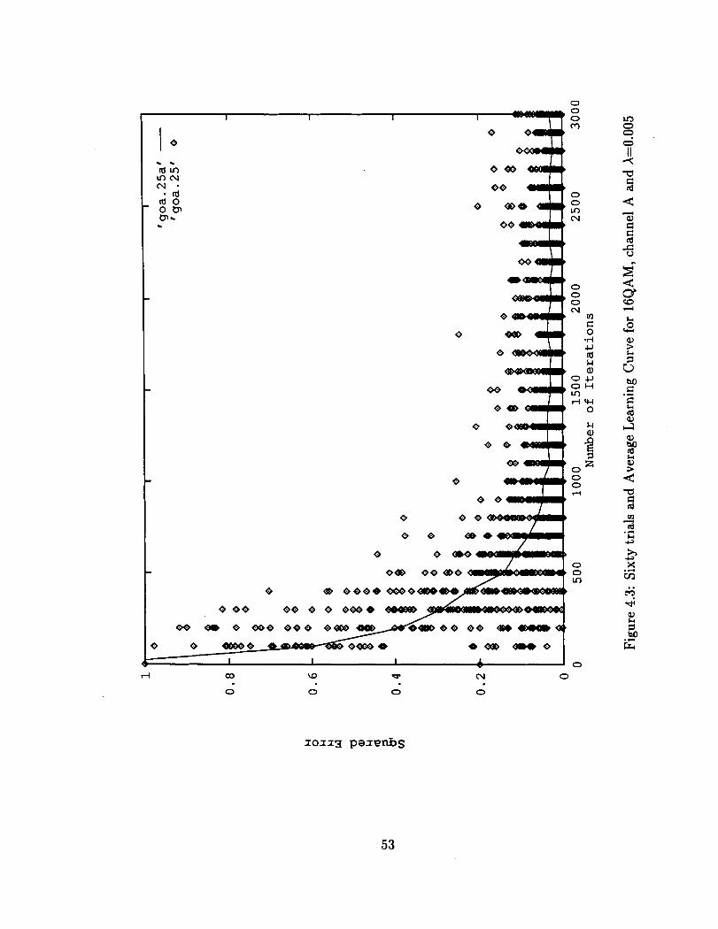
4.3 Sixty trials and Average Learning Curve for 16QAM. channel A and
A=0.005 . . . . . . . . . . . . . . . . . . . . . . . . . . . . . . . . . . 53
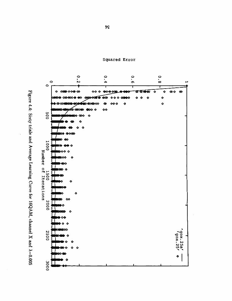
4.4 Sixty trials and Average Learning Curve for 16QAM. channel X and
A=0.005 . . . . . . . . . . . . . . . . . . . . . . . . . . . . . . . . . . 54
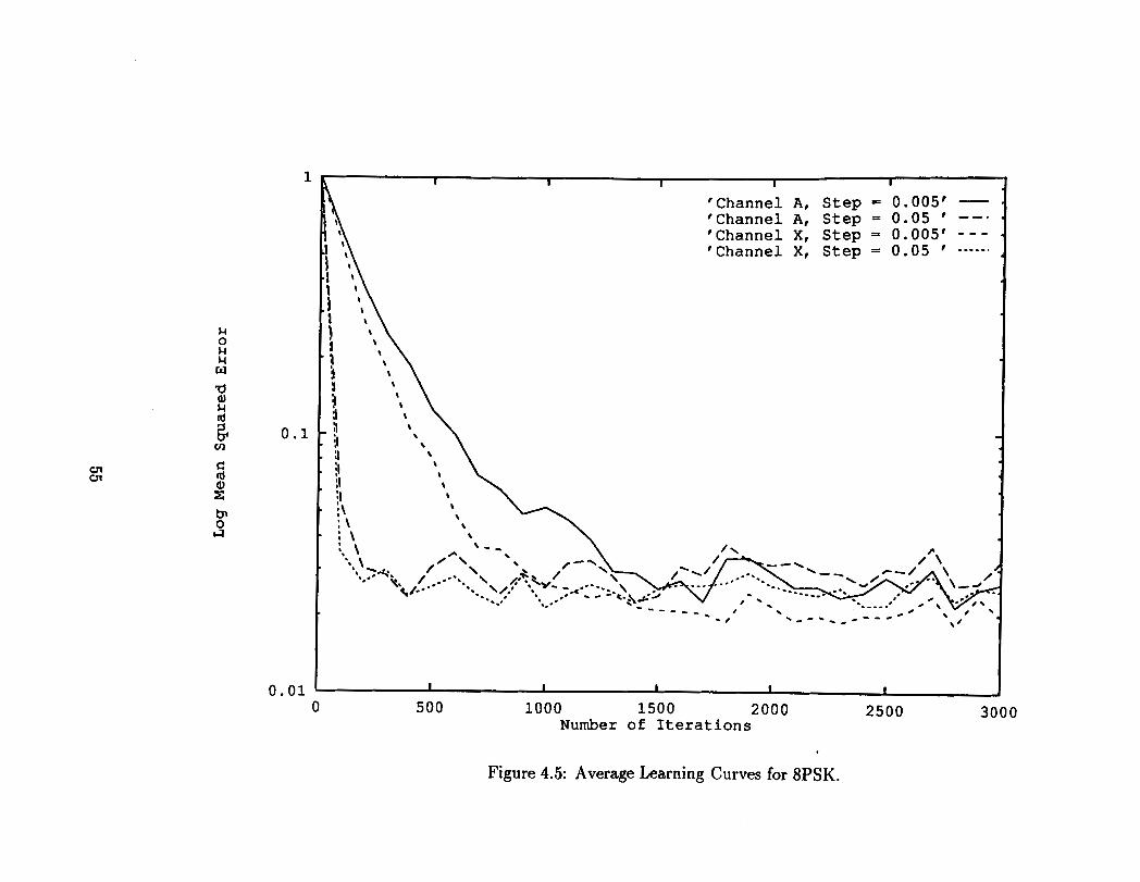
. . . . . . . . . . . . . . . . . . . . 4.5 Average Learning Curves for 8PSK 55
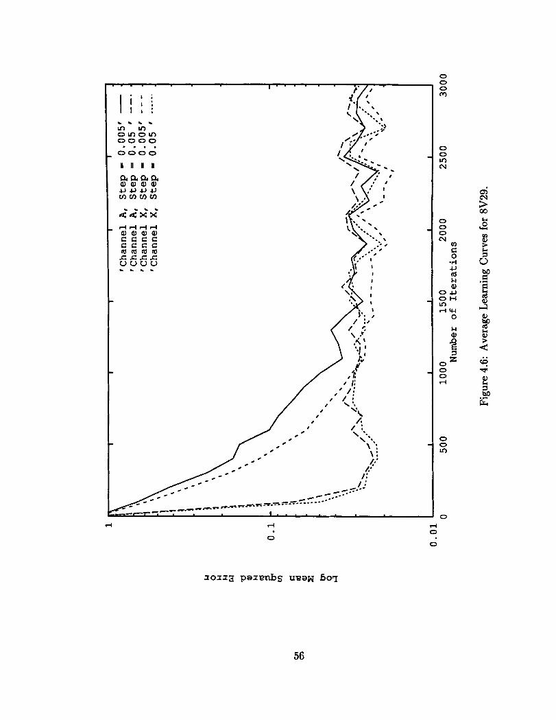
4.6 Average Learning Curves for 8V29 . . . . . . . . . . . . . . . . . . . . 56
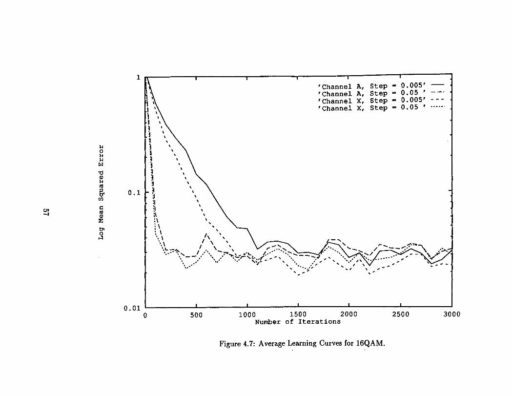
4.7 Average Learning Curves for 16QAM . . . . . . . . . . . . . . . . . . . 57
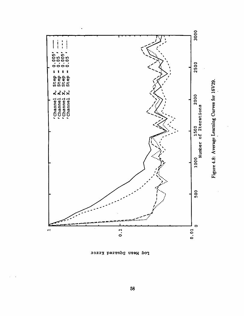
4.8 Average Learning Curves for 16V29 . . . . . . . . . . . . . . . . . . . 58
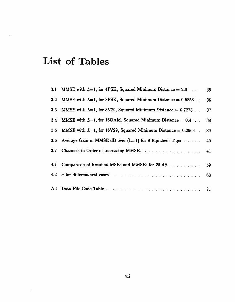
List of Tables
3.1 MMSE with L=l, for 4PSK, Squared Minimum Distance = 2.0 . . . 35
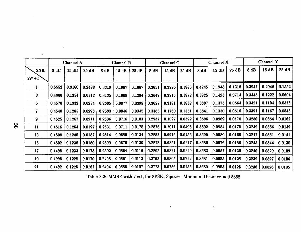
3.2 MMSE with L=l, for 8PSK, Squared Minimum Distance = 0.5858 . . 36
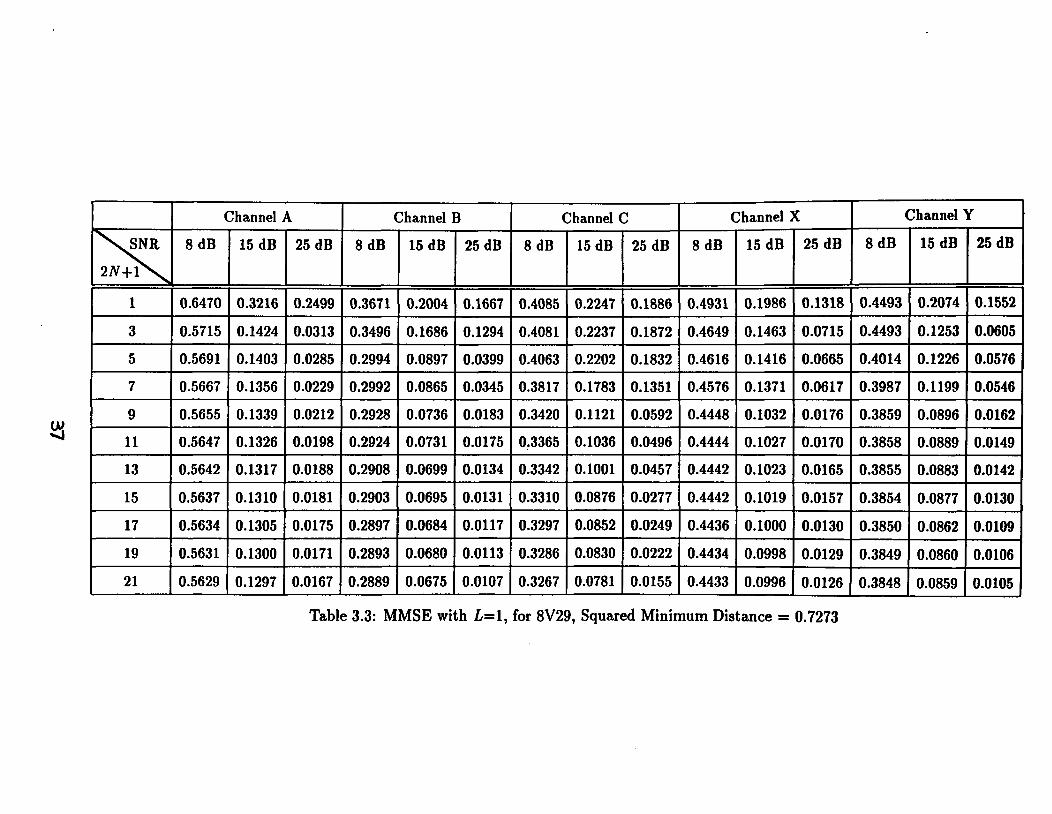
3.3 MMSE with L=l, for 8V29, Squared Minimum Distance = 0.7273 . . 37
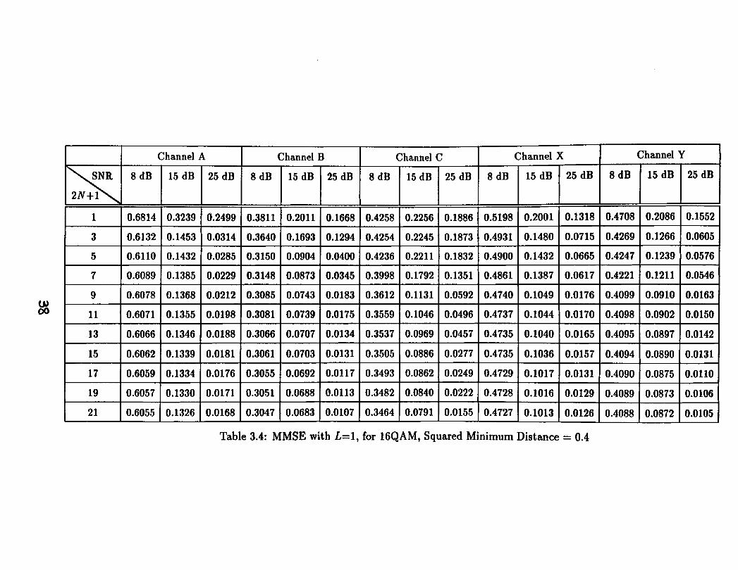
3.4 MMSE with L=l, for 16QAM, Squared Minimum Distance = 0.4 . . 38
3.5 MMSE with L=l, for 16V29, Squared Minimum Distance = 0.2963 . 39
3.6 Average Gain in MMSE dB over (L=l) for 9 Equalizer Taps . . . . . 40
3.7 Channels in Order of Increasing MMSE. . . . . . . . . . . . . . . . . 41
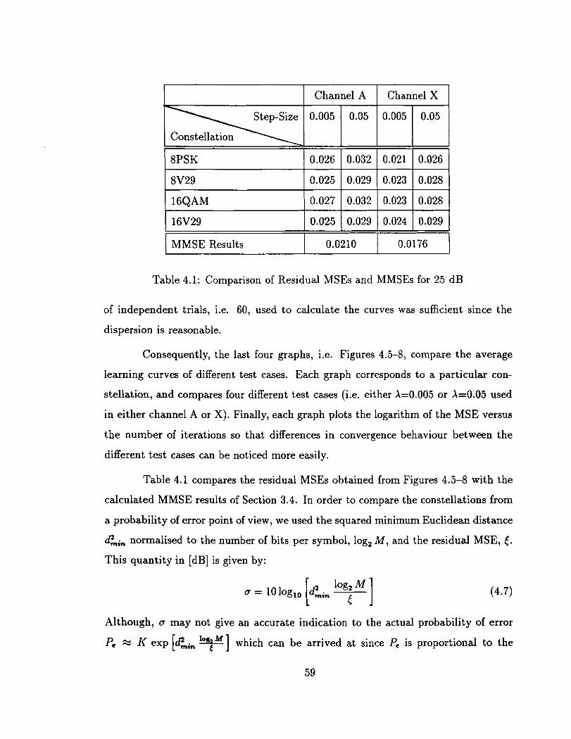
4.1 Comparison of Residual MSEs and MMSEs for 25 dB . . . . . . . . . 59
4.2 a for different test cases . . . . . . . . . . . . . . . . . . . . . . . . . 60
A.l Data File Code Table . . . . . . . . . . . . . . . . . . . . . . . . . . . 71
vii
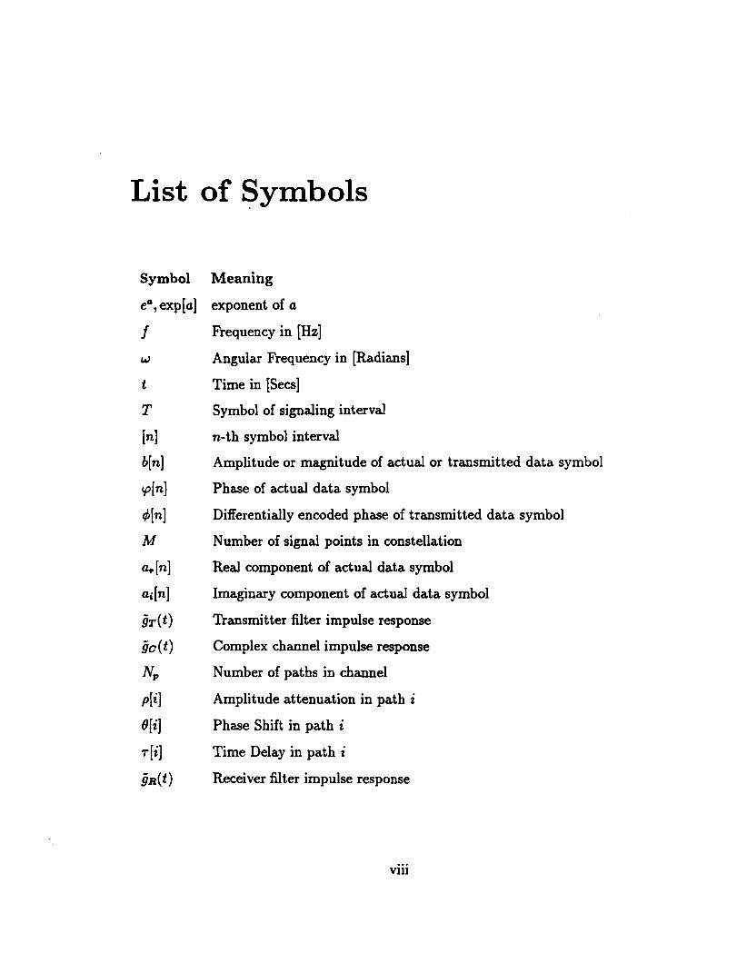
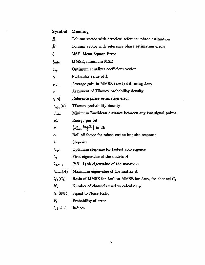
List of Symbols
Meaning
exponent of a
Frequency in [Hz]
Angular Frequency in [Radians]
Time in [Secs]
Symbol of signaling interval
n-th symbol interval
Amplitude or magnitude of actual or transmitted data symbol
Phase of actual data symbol
Differentially encoded phase of transmitted data symbol
Number of signal points in constellation
Real component of actual data symbol
Imaginary component of actual data symbol
Transmitter filter impulse response
Complex channel impulse response
Number of paths in channel
Amplitude attenuation in path i
Phase Shift in path i
Time Delay in path i
Receiver filter impulse response
. . . Vll l
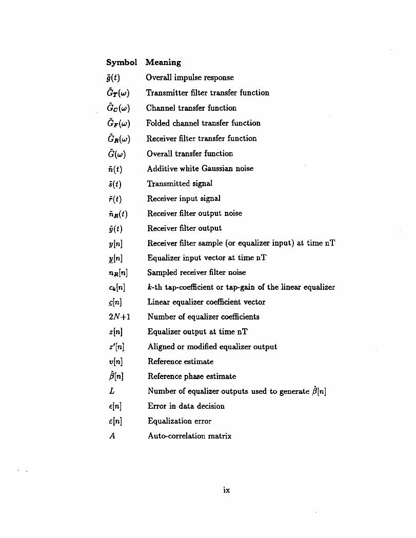
Meaning
Overall impulse response
Transmitter filter transfer function
Channel transfer function
Folded channel transfer function
Receiver filter transfer function
Overall transfer function
Additive white Gaussian noise
Transmitted signal
Receiver input signal
Receiver filter output noise
Receiver filter output
Receiver filter sample (or equalizer input) at time nT
Equalizer input vector at time nT
Sampled receiver filter noise
k-th tap-coefficient or tap-gain of the linear equalizer
Linear equalizer coefficient vector
Number of equalizer coefficients
Equalizer output at time nT
Aligned or modified equalizer output
Reference estimate
Reference phase estimate
Number of equalizer outputs used to generate &n]
Error in data decision
Equalization error
Auto-correlation matrix
A 2 ~ + 1
&7(Ci)
N c
A, SNR
pe
i , i k, 1
Meaning
Column vector with errorless reference phase estimation
Column vector with reference phase estimation errors
MSE, Mean Square Error
MMSE, minimum MSE
Optimum equalizer coefficient vector
Particular value of L
Average gain in MMSE (L=l) dB, using L=y
Argument of Tikonov probability density
Reference phase estimation error
Tikonov probability density
Minimum Euclidean distance between any two signal points
Energy. per bit
(tin ) in d~
Roll-off factor for raised-cosine impulse response
Step-size
Optimum step-size for fastest convergence
First eigenvalue of the matrix A
(2 N + 1 )-th eigenvalue of the matrix A
Maximum eigenvalue of the matrix A
Ratio of MMSE for L=l to MMSE for L=r, for channel C;
Number of channels used to calculate p
Signal to Noise Ratio
Probability of error
Indices
Chapter 1
Introduction
Recent years have witnessed an increased interest in bandwidth efficient modulation
schemes. The simplest and most widely used technique for achieving high bandwidth
efficiency is based on two-dimensional modulation formats 111. With these schemes,
demodulation is usually performed coherently, which means that carrier phase track-
ing is necessary. In many situations (such .as communication over fading multipath
channels, or short burst communications such as TDMA or Frequency Hopping), car-
rier phase tracking is a difficult task, and thus noncoherent demodulation techniques
have to be used. The noncoherent demodulation methods for two-dimensional formats
are based on differentially coherent techniques, and thus the phase information has
to be differentially encoded. In these schemes, carrier phase tracking is not necessary;
however, this is achieved at the expense of SNR performance.
In the last year, new differentially coherent detection techniques have been
introduced [2]-[5]. The chief merit of these detection schemes is their low SNR degra-
dation with respect to corresponding coherent detectors. One of the potential appli-
cations of the new differentially coherent strategies is for Indoor Wireless and Mobile
Communications. In these systems, intersymbol interference due to multipath is a
major problem. Therefore, the extent to which the new differentially coherent de-
tection techniques can be suitable for these applications depends on the performmce
of these schemes in an intersymbol interference environment, and the possibility of
combining them with equalization. This subject has not been considered yet (as far
as we know), and this work makes a first step in this direction.
Two-dimensional modulation, where the data is encoded into the phase and
amplitude of a sinusoidal carrier has been extensively studied in [I], (61-[ll]. In this
work, Phase Shift Keying (PSK), Quadrature Amplitude Modulation (QAM) and
V29 signal constellations [12], [13, page 2431 will be used in a combined amplitude
and differential phase modulation scheme, which uses amplitudes and phase differ-
ences to convey information. This modulation scheme is used instead of combined
amplitude and phase modulation because the differential phase encoding enables the
use of differentially coherent detection. Differentially coherent detection simplifies
the receiver structure significantly since no phase tracking is performed and thus,
is very attractive when carrier phase tracking is difficult. However, it has an SNR
performance degradation compared to coherent detection that approaches 3 dB for
,MPSK ( M > 2 ) . As a result, we propose to use the decision-feedback differentially
coherent detection structure of [2] because of its low SNR degradation and relatively
low complexity. Our objective is to consider this scheme over IS1 channels, while
focusing on the multipath environment. The decision-feedback differentially coherent
detector of [2] can be naturally combined with known equalization techniques, while
the other proposed differentially coherent detectors [3]-[5], seem to require special
equalization methods.
In this work, we consider linear equalization, because of its reduced complex-
ity. In addition, the Mean-Square-Error (MSE) criterion is used to find the optimum
linear equalizer for known channels. However, in practice, the multipath characteris-
tics of these channels are usually not known so that adaptive equalization is necessary.
Therefore, we also consider the Least-Mean-Squares (LMS) adaptation algorithm [14],
mainly because of its simplicity and robustness and also because it is one of the more
popular algorithms used in practice.
This thesis is organized along the following lines. Chapter 2 presents the
rationale of combining linear equalization with decision-feedback differentially coher-
ent detection, and introduces the system model. In Chapter 3, the minimum MSE
(MMSE) and optimum equalizer coefficients are derived for known channels, taking
into account reference phase errors, and numerical results are presented for some mul-
tipath channels. In Chapter 4, the LMS adaptive algorithm is used for adapting the
equalizer to an unknown channel and Adaptive Mean-Square-Error (AMSE) simu-
lation results are presented. Finally, Chapter 5 states the conclusions and suggests
further work. This is followed by a bibliography of related articles and two appen-
dices. Appendix A presents an overview of the overall computer program and lists
the MMSE program file and a sample test case. Appendix B lists the AMSE program
file, a sample test case and additional program files.
Chapter 2
Combining Equalization. and
Decision-Feedback Differentially
Coherent Detection
The subject of this chapter is the integration of linear equalization with differentially
coherent detection. Section 2.1 discusses the need for differentially coherent detection
and linear equalization in a communication system. Section 2.2 describes the base-
band system model, including the proposed receiver which combines an improved
differentially coherent detection structure with a linear equalizer. Finally, Section
2.3 focuses on the advantages of this proposed receiver over conventional coherent
receivers which combine coherent detection and linear equalization.
Equalization and Decision-Feedback Differen-
tial Coherent Detection
Any communication system consists of three components: transmitter, channel and
receiver. The main objective in any communication system is to transmit information
as accurately as possible. The transmitter encodes the discrete-time information into
a continuous-time signal which is transmitted over the channel. The receiver must
recover the information from the received signal which is a distorted version of the
transmitted signal. This distortion is due to the channel. Channel distortion can be
generated by noise, fading, as well as time-dispersion. Therefore, the transmitter and
receiver have to be designed with the communications channel in mind.
An important parameter of a communication system is the method by which
the information is encoded into the transmitted signal, the modulation method. Much
attention has been given to two-dimensional modulation, where the data is encoded
into the phase and amplitude of a sinusoidal carrier [6]-[8], mainly because of its
bandwidth efficiency. A close relative to this amplitude and phase modulation is
amplitude and differential phase modulation.
Differential phase modulation structures the sinusoidal carrier such that car-
rier phase differences and not actual carrier phases convey information [15]. Thus,
carrier phase tracking, which tracks absolute phases, is not necessary at the receiver
since phase differences between successive signals (and not the absolute phases of the
signals) convey information. The phase encoding adds little to the complexity of the
transmitter. In this work, combined amplitude and differential phase modulation,
with differentially coherent detection, is considered.
A differentially coherent detector estimates the transmitted information by
making use of phase differences between successive symbols. In the absence of channel
distortion, differentially coherent detection is an attractive alternative to coherent
detection especially when carrier phase recovery is difficult. It has been successfully
applied with PSK modulation, particularly for binary PSK (BPSK) signal [16, page
1741. This gives an extremely simple receiver for BPSK with a small degradation
in performance. However, for MPSK (M>2), it gives an SNR degradation that
approaches 3 dB as M increases. In [2], an improved differentially coherent detection
technique was introduced. The proposed differential receiver structure uses past phase
decisions to modify L previous received samples. These modified samples were then
summed to give an improved phase reference. This strategy can be considered as an
open loop version of a coherent receiver with decision-feedback carrier phase tracking.
It was found that the performance of this improved differentially coherent detection
approaches that of coherent detection for high SNR.
As stated earlier, the channel distorts the transmitted signal. In a time-
dispersive channel, the effect of each transmitted symbol extends beyond the time-
interval used to represent that symbol. This is due to the dispersion effect of the
channel which broadens pulses and causes them to interfere with one another. The
distortion caused by the resulting overlap of received signals is called intersymbol
interference (ISI). Its effect is most easily described in an equivalent baseband pulse
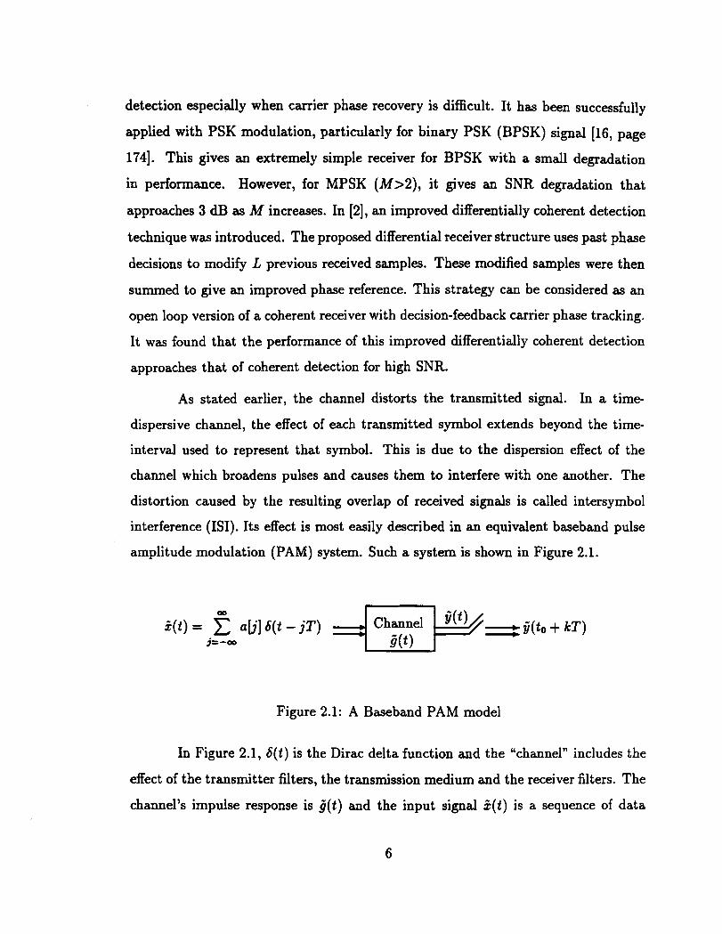
amplitude modulation (PAM) system. Such a system is shown in Figure 2.1.
Channel - 2 a b ] 6(t - jT) 4 j(t) tm/T kT) Z(t) - j=-a0
Figure 2.1: A Baseband PAM model
In Figure 2.1, 6(t) is the Dirac delta function and the "channeln includes the
effect of the transmitter filters, the transmission medium and the receiver filters. The
channel's impulse response is j(t) and the input signal 5(t) is a sequence of data
symbols alj] which are transmitted at instants jT through the channel where T is the
signaling (or symbol) interval and is used to represent the complex envelope (CE)
notation. Therefore, the CE of the received signal g(t) is given by
If the received signal is sampled at instant kT +to, where to accounts for the channel
delay and the sampler phase, we get
The IS1 is induced by )(to + iT), i # 0. The IS1 is zero if )(to + iT)=O, i # 0; that is,
if #(t) has zero crossings at T-spaced intervals. When @(t) has such uniformly spaced
zero crossings, it is said to satisfy Nyquist's criterion [13, page 1571. The criterion
specifies a frequency-domain condition on the received pulses for zero ISI. It can be
expressed as: OD k 1 e ~ ( f ) = &(f - T ) = T for i f 1 5 -
&=-w 2T
where e ( f ) is the channel frequency response (i-e. the Fourier transform of jj(t)),
c ~ ( f ) is the folded channel spectral response after symbol-rate sampling and the
frequency band 1 f 1 5 5 is the Nyquist or minimum bandwidth.
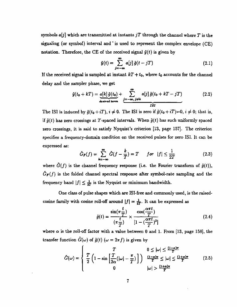
One class of pulse shapes which are ISI-free and commonly used, is the raised-
cosine family with cosine roll-off around 1 f 1 = &. It can be expressed as
where a is the roll-off factor with a value between 0 and 1. From [13, page 1581, the
transfer function ~ ( w ) of )(t) (w = 2n f ) is given by
T T &(w) = ( 5 (I - sin [20(lui - j)] )
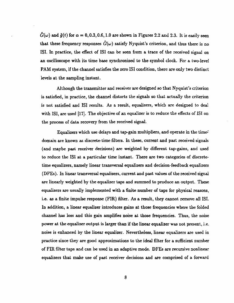
G(w) and j ( t ) for a = 0,0.3,0.6,1.0 are shown in Figures 2.2 and 2.3. It is easily seen
that these frequency responses ~ ( w ) satisfy Nyquist's criterion, and thus there is no
ISI. In practice, the effect of IS1 can be seen from a trace of the received signal on
an oscilloscope with its time base synchronized to the symbol clock. For a two-level
PAM system, if the channel satisfies the zero IS1 condition, there are only two distinct
levels at the sampling instant.
Although the transmitter and receiver are designed so that Nyquist's criterion
is satisfied, in practice, the channel distorts the signals so that actually the criterion
is not satisfied and IS1 results. As a result, equalizers, which are designed to deal
with ISI, are used [17]. The objective of an equalizer is to reduce the effects of IS1 on
the process of data recovery from the received signal.
Equalizers which use delays and tap-gain multipliers, and operate in the time:
domain are known as discrete-time filters. In these, current and past received signals
(and maybe past receiver decisions) are weighted by different tap-gains, and used
to reduce the IS1 at a particular time instant. There are two categories of discrete-
time equalizers, namely linear transversal equalizers and decision-feedback equalizers
(DFEs). In linear transversal equalizers, current and past values of the received signal
are linearly weighted by the equalizer taps and summed to produce an output. These
equalizers are usually implemented with a finite number of taps for physical reasons,
i.e. as a finite impulse response (FIR) filter. As a result, they cannot remove all ISI.
In addition, a linear equalizer introduces gains at those frequencies where the folded
channel has loss and this gain amplifies noise at those frequencies. Thus, the noise
power at the equalizer output is larger than if the linear equalizer was not present, i.e.
noise is enhanced by the linear equalizer. Nevertheless, linear equalizers are used in
practice since they are good approximations to the ideal filter for a sufficient number
of FIR filter taps and can be used in an adaptive mode. DFEs are recursive nonlinear
equalizers that make use of past receiver decisions and are comprised of a forward
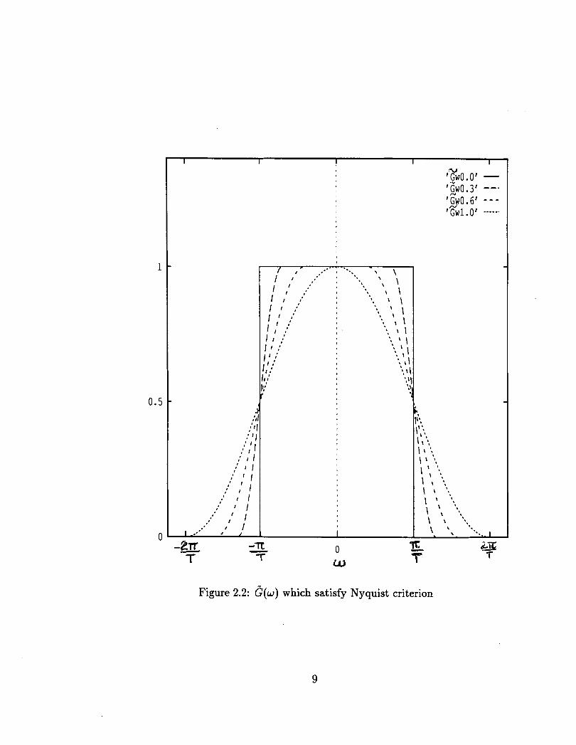
Figure 2.2: e ( w ) which satisfy Nyquist criterion
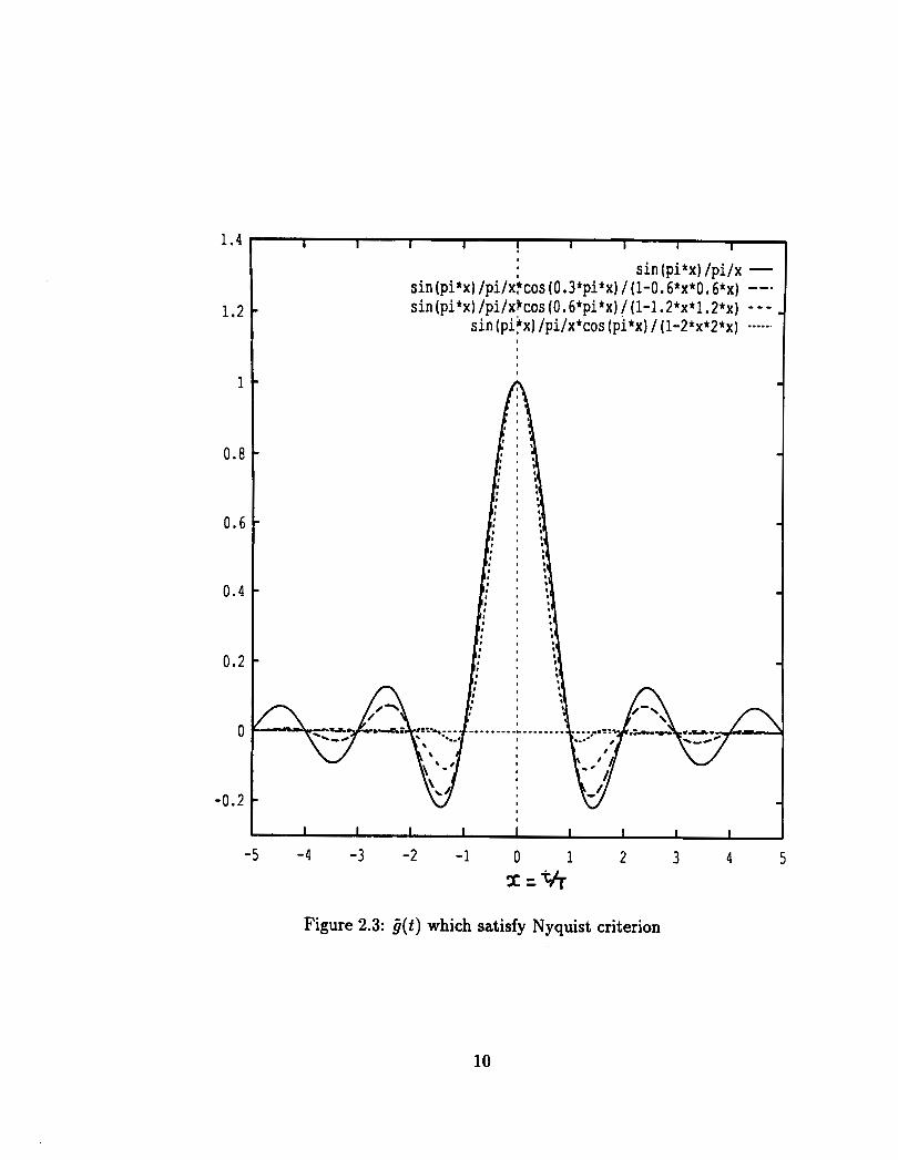
sin (pi*x) /pi/x - sin (pi*x) /pi/x?cos (0.3*pi*x) / (1-0.6*x*O. 6 ) --- sin (pi*~) /pi/xkos (0.6*pi*x) /(I-1.2*x*1.2*~) - - -
sin (pitx) /pi/x*cos (pi*x) / (1-2*x*2*x) -----.
Figure 2.3: g ( t ) which satisfy Nyquist criterion
and feedback filter. The forward filter is similar to a linear transversal filter. Its
function is to eliminate precursor IS1 (samples of the pulse response before the main
lobe) while the function of the feedback filter is to cancel the postcursor IS1 (samples
of the pube response after the main lobe), see Figure 2.3. In addition, DFEs do not
enhance noise as much as linear equalizers and are less sensitive to sampling phase
errors. However, DFEs suffer from feedback error propagation. Therefore, they are
more difficult to use in adaptive mode due to this lack of guaranteed stability.
This work considers linear equalization for systems that employ different ial
detection. This subject has been given consideration in the literature [15], [18]-[20].
A linear equalizer following a differential detector as in [18], has the difficult task
of equalizing a nonlinear channel due to the quadratic nature of the channel depen-
dent terms at the differential detector output. As a result, a linear equalizer cannot
effectively equalize the channel, and non-linear equalization techniques should be con-
sidered. Therefore, a linear equalizer should precede the differential detector as in [15],
since it has to equalize a linear channel. In [19], a scheme for adaptive equalization
of incoherently demodulated signals was presented. In the scheme, a linear equalizer,
placed after an envelope detector, was used to make an estimate of the IS1 due to
multipath fading and acted as an IS1 canceller (i.s.i.c). In addition, differential phase
estimation and phase tracking estimation were both used in the receiver structure.
Also, the equalizer structure had complex tap-gains and real input values, instead of
the usual complex tap gains and complex input values, which reduced the system com-
plexity by fifty percent. However, in this scheme, the linear equalizer has the difficult
task of coping with the nonlinearity introduced by the envelope detector. Adaptive
equalization for differential coherent reception in the presence of channel distortion
was also studied in (201. A linear equalizer, with seven taps, was placed before a
differential detector and differential data encoding was performed by multiplying the
previously transmitted data symbol by the current data symbol. Simulations were
done at high SNR for BPSK and QPSK. Similar rates of convergence were shown for a
coherent receiver and the differential detection receiver. However, the MSE obtained
for the differential case was about 3 dB larger than that obtained in the coherent
case. We intend to solve this problem by using the improved differentially coherent
detection technique of [2].
In [2], an improved differentially coherent detection receiver was introduced
for an ISI-free additive white Gaussian noise channel. The main advantage of this
differentially coherent detection technique is its negligible degradation with respect
to coherent detection. With ISI, there is need for an equalizer as well. By placing
a linear equalizer before differentially coherent detection, the effects of the IS1 can
be reduced and detection is performed on an almost ISI-free signal. Furthermore,
equalization is performed without the need for carrier phase tracking, improving the
robustness of the system to carrier phase noise, and carrier phase hits.
2.2 Baseband System Model
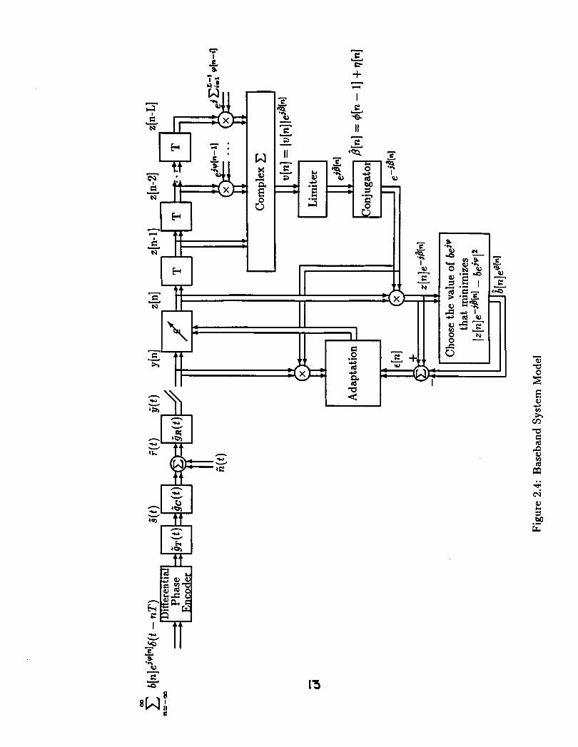
The baseband model (complex envelope) for the system considered in this work is
shown in Figure 2.4. In this work, continuous-time signals use ( ) brackets and
discrete-time signals [ ] rectangular brackets. Figure 2.4 will now be briefly described:
The system is composed of three conceptual parts: transmitter, channel and receiver.
2.2.1 Transmitter
The transmitter model consists of a differential phase encoder followed by a trans-
mitter filter # ~ ( t ) . Let us consider two dimensional modulated data signals specified
by the complex envelope (CE) notation. The CE of the transmitted signal is given
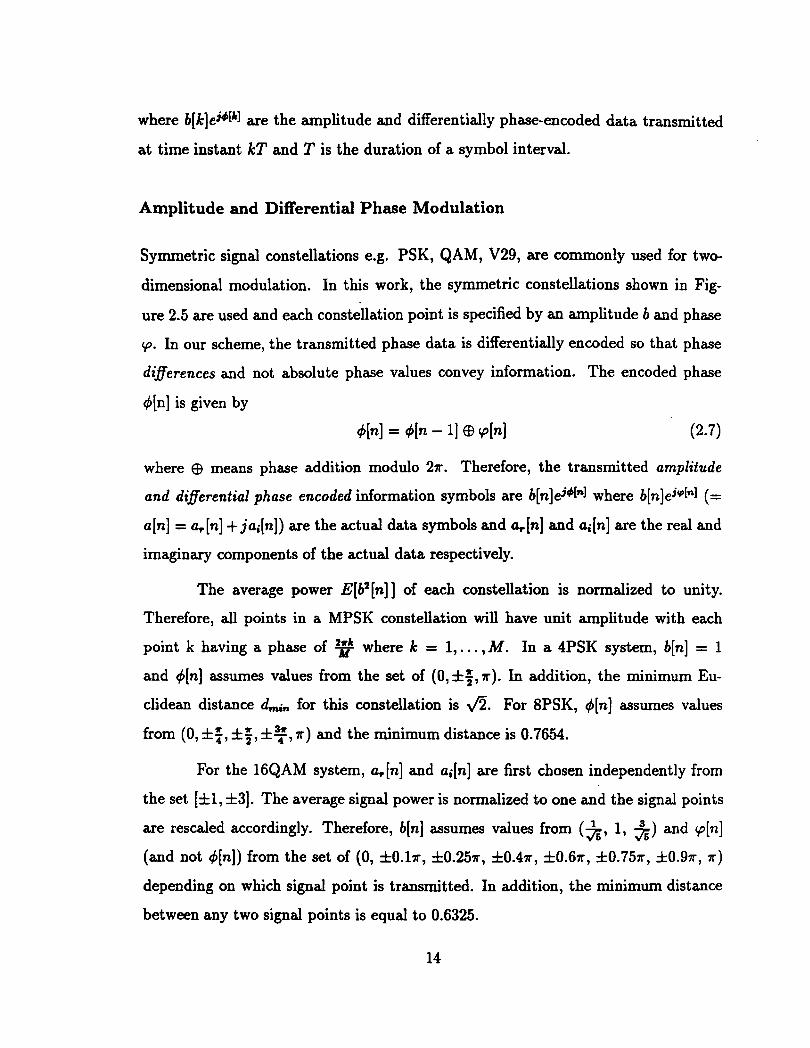
where b[k]ej4ih] are the amplitude and differentially phase-encoded data transmitted
at time instant kT and T is the duration of a symbol interval.
Amplitude and Differential Phase Modulation
Symmetric signal constellations e.g. PSK, QAM, V29, are commonly used for two-
dimensional modulation. In this work, the symmetric constellations shown in Fig-
ure 2.5 are used and each consteilation point is specified by an amplitude b and phase
cp. In our scheme, the transmitted phase data is differentially encoded so that phase
differences and not absolute phase values convey information. The encoded phase
4[n] is given by
where $ means phase addition modulo 2n. Therefore, the transmitted amplitude
and differential phase encoded information symbols are b[n]ej4["1 where b[n]ej'["l (=
a[.] = ar[n] + jai[n]) are the actual data symbols and a,[n] and ai[n] are the real and
imaginary components of the actual data respectively.
The average power E[b2[n]] of each constellation is normalized to unity.
Therefore, all points in a MPSK constellation will have unit amplitude with each
point k having a phase of where k = 1,. . . , M. In a 4PSK system, b[n] = 1
and 4[n] assumes values from the set of (0, f $,r). In addition, the minimum Eu-
clidean distance kin for this constellation is fi. For 8PSK, 4[n] assumes values
from (0, ztq, f y , *?, T ) and the minimum distance is 0.7654.
For the 16QAM system, a,[n] and ai[n] are first chosen independently from
the set [f 1, f 31. The average signal power is normalized to one and the signal points
are rescaled accordingly. Therefore, b[n] assumes values from (5, 1, 5) and ~ [ n ]
(and not +[n]) from the set of (0, f O.ln, f O.257r, f OAT, f O.6n, f O.75n, f O.gn, n)
depending on which signal point is transmitted. In addition, the minimum distance
between any two signal points is equal to 0.6325.
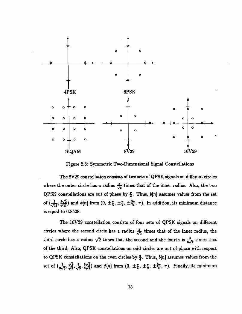
Figure 2.5: Symmetric Two-Dimensional Signal Constellations
The 8V29 constellation consists of two sets of QPSK signals on different circles
where the outer circle has a radius 5 times that of the inner radius. Also, the two
QPSK constellations are out of phase by f . Thus, b[n] assumes values from the set
p) and 4[n] from (0, f 2, f f, f F, r). In addition, its minimum distance (7% n is equal to 0.8528.
The 16V29 constellation consists of four sets of QPSK signals on different
circles where the second circle has a radius 5 times that of the inner radius, the
third circle has a radius 4 times that the second and the fourth is & times that
of the third. Also, QPSK constellations on odd circles are out of phase with respect
to QPSK constellations on the even circles by Q. Thus, b[n] assumes values from the
set of (&, $,&, 3) and 4[n] from (0, f f , f f , f F, r). Finally, its minimum
distance is equal to 0.5443.
Transmitter Filter
The transmitter filter is a pulse shaping filter with a real impulse response ijT ( t ) . The
desired overall impulse response j ( t ) (= jT( t ) *#c ( t ) * j ~ ( t ) where * denotes convolu-
tion.) is a Nyquist raised-cosine response with roll-off factor a, assuming ijc(t) = 6(t) .
Also, the transfer function of the desired Nyquist raised-cosine response is divided
equally between the transmitter and the receiver filters. Thus, the transmitter filter
is designed so that its transfer function &(w) is equal to dm where &(w) is the
transfer function of the desired Nyquist response #( t ) . In our model, the roll-off factor
cr is set to zero so that the raised-cosine Nyquist response has zero excess-bandwidth.
Therefore, the transmitter's impulse response aT ( t )
and the transfer function GT(w) is given by
can be expressed as:
2.2.2 Channel
The channel response is represented by the complex impulse response j c ( t ) and ad-
ditive white Gaussian noise i i( t) . A multipath channel model is used. Thus, the
complex impulse response j c ( t ) can be expressed as
where Np is the number of paths in the channel, p[i ] is the amplitude attenuation in
path i, B[i] is the phase-shift in path i and ~ [ i ] is the relative signal delay due to path
i. Consequently, the receiver input, +(t) can be expressed as
where s'(t) is the transmitted signal, ijc(t) is the channel impulse response and fi(t)
is additive white Gaussian noise with zero-mean and No [Watt/Hz] power spectral
density of the real and imaginary component.
2.2.3 Receiver
The baseband equivalent receiver consists of a filter with impulse response jR(t)
followed by a sampler. The sampler is followed by a linear equalizer and then by the
decision-feedback differential coherent detection structure of [2].
Receiver Filter
As previously stated, the transmitter and receiver filters are designed so that the
overall response in an ideal channel is a Nyquist raised-cosine response. In addition,
the desired Nyquist transfer function is divided equally between the two filters, which
gives an optimal receiver structure for an ISI-free channel. Thus, the receiver filter
has transfer function GR(u) which is given by
where GT(w) is the transfer function of the transmitter filter impulse response, which
is given in (2.9) and ~ ( w ) is the transfer function of the desired overall response.
Using (2.11), the receiver filter output g(t) is given by
where S ( t ) is the transmitted signal, ac(t) is the channel impulse response, fi(t) is the
channel additive white Gaussian noise and ijR(t) is the receiver filter impulse response.
Thus, the receiver filter output can also be expressed as
where
and
Therefore, the noise fiR(t) has zero-mean and power spectrum density
where GR(w) denotes the Fourier transform of jR( t ) . Sampling the received signal
g( t ) at t = n T , the discrete-time output y [n] can be expressed as:
OD
[n] = b[k]ei4(lIg[n - k] + nR[n] (2.16) k = - O D
where g[n - k] = j ( [ n - k ] T ) , nR[n] = fiR(nT) and b[k]ej41k] are the amplitude and
differentially phase-encoded data transmitted at time instant kT.
Linear Equalizer
The linear equalizer has 2N+1 complex taps and equalizes both in-phase and quadra-
ture components using its real and imaginary taps. The input to the linear equal-
izer is given in (2.16). The adaptive digital equalizer has complex coefficients ck[n]:
k = -N , . . . ,O,. . . , N where ~ [ n ] is the reference tap and [n] corresponds to a par-
ticular symbol interval or iteration. Thus, the equalizer output +] is given by:
There are many criteria for obtaining the optimum linear equalizer coefficients for a
known channel. The peak distortion criterion would have been sufficient if only the
IS1 is to be minimized [21]. However, the noise must be taken into account. Therefore,
the Mean Square Error(MSE) criterion is used.
For an unknown or time-varying channel, the equalizer must adapt itself. The
speed and stability of convergence are important factors which must be considered
in choosing an adaptive algorithm. In fact, many different adaptive algorithms exist
and a survey on adaptive equalization can be found in [22]. One adaptive algorithm
is the Least-Mean-Squares (LMS) gradient algorithm, which was proposed in [14] and
has been extensively used in the last few decades. In this work, the LMS algorithm
is employed because of its simplicity and robustness and is the subject of Chapter
4. Finally, there has been recent work on faster-converging algorithms [23]-[25], and
these algorithms are briefly discussed in Chapter 4.
Decision-Feedback Differentially Coherent Detection
We use an improved differentially coherent detection structure, introduced in (21 which
can reduce the SNR degradation with respect to coherent detection. The principles
on which this detection strategy rely on will now be discussed.
One way of interpreting a differentially encoded scheme is in terms of phase
references. Differential phase encoding preprocesses the signal such that the required
phase reference for estimating the information is carried by the previous symbol.
Therefore, in differentially coherent detection, there is no need to establish an absolute
phase reference, since the previous symbol phase is used for that. This simplifies
the receiver structure when compared to coherent detection which requires carrier
phase tracking. However, this is achieved at the expense of a loss of about 3 dB in
performance relative to coherent MPSK(M> 2). This is because in a differentially
coherent (DC) scheme, the phase reference is impaired hy channel noise in the same
way as the information phase. Therefore, in a DC scheme, detection is performed with
a noisy phase reference, and when compared to ideal coherent detection, where the
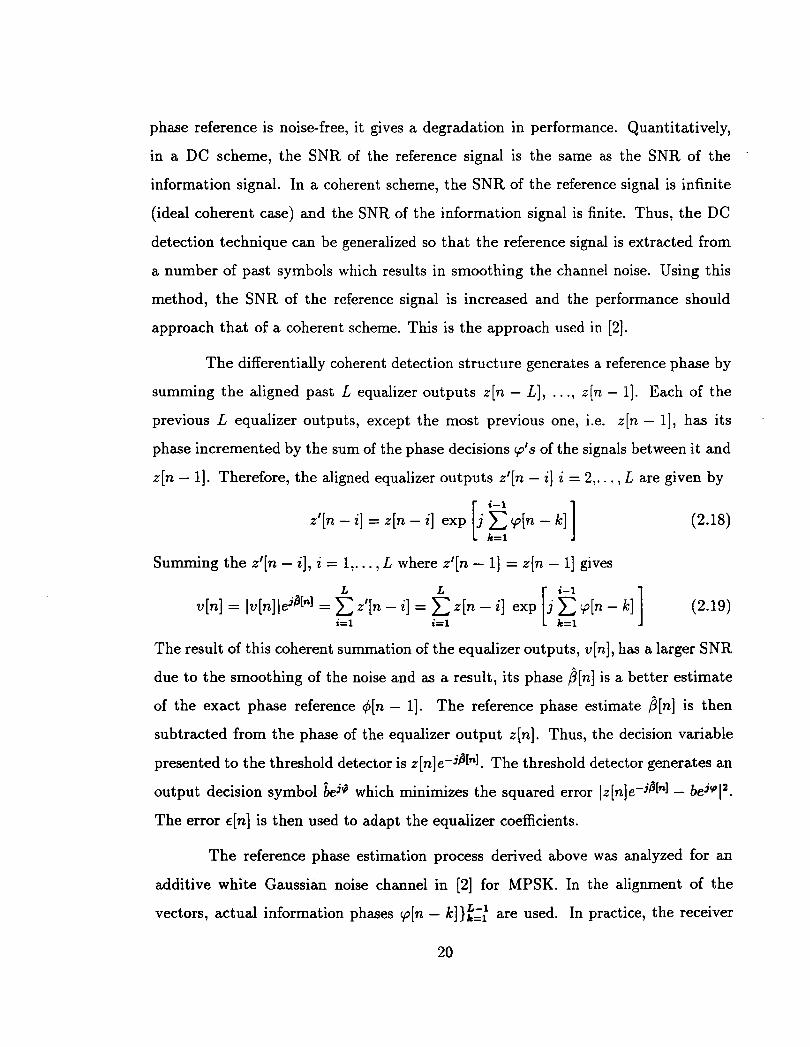
phase reference is noise-free, it gives a degradation in performance. Quantitatively,
in a DC scheme, the SNR of the reference signal is the same as the SNR of the
information signal. In a coherent scheme, the SNR of the reference signal is infinite
(ideal coherent case) and the SNR of the information signal is finite. Thus, the DC
detection technique can be generalized so that the reference signal is extracted from
a number of past symbols which results in smoothing the channel noise. Using this
method, the SNR of the reference signal is increased and the performance should
approach that of a coherent scheme. This is the approach used in [2].
The differentially coherent detection structure generates a reference phase by
summing the aligned past L equalizer outputs z[n - L], . . ., z[n - 11. Each of the
previous L equalizer outputs, except the most previous one, i.e. z[n - 11, has its
phase incremented by the sum of the phase decisions cp's of the signals between it and
z[n - 11. Therefore, the aligned equalizer outputs zt[n - i] i = 2,. . . , L are given by
i-1
zt[n - i] = z[n - i] exp
Summing the z' [n - i], i = 1 ,. . . , L where z'[n - 11 = z[n - 11 gives
L L i-1
t~ [n] = 1 v [n] 1 eie["] = x z'[n - i] = z [n - i] exp I j x y [n - k]
The result of this coherent summation of the equalizer outputs, v[n], has a larger SNR
due to the smoothing of the noise and as a result, its phase p[n] is a better estimate
of the exact phase reference q5[n - 11. The reference phase estimate b[n] is then
subtracted from the phase of the equalizer output z[n]. Thus, the decision variable
presented to the threshold detector is z[n]e-jfi["]. The threshold detector generates an
output decision symbol k j h h i c h minimizes the squared error ( r [n] e-jBln] - bej'12.
The error ~ [ n ] is then used to adapt the equalizer coefficients.
The reference phase estimation process derived above was analyzed for an
additive white Gaussian noise channel in [2] for MPSK. In the alignment of the
vectors, actual information phases cp[n - k]):;: are used. In practice, the receiver
operates in a decision-feedback mode (i.e. cp's used in the alignment process would be
the $ decisions on previous phases). To simplify the analysis, the feedback decisions
are assumed error-free. The effect of errors in the feedback decisions would be to
reduce momentarily the SNR of the reference signal which obviously depends on L.
For small L, a decision-feedback error is more noticeable. However, the persistence
time of this effect is only L symbols and is thus short. For L=l, this is just the
double error effect in DC receivers. For large L, a decision-feedback error is not very
noticeable since the SNR reduction in the reference signal is small. However, the
effect lasts for L symbols.
Comparison with Equalization and Coherent
Detection
The advantages of our "differentialn receiver, which combines an improved differen-
tially coherent detection scheme and linear equalization, over conventional "coherentn
receivers, which combine coherent detection and equalization, will now be discussed.
The first advantage of the differential receiver is that it can be used in fading
multipath channels where carrier phase tracking is difficult. This is because the
proposed differential receiver avoids carrier phase tracking with little performance
degradation. If a coherent receiver were employed, carrier phase tracking would be
quite complicated since carrier phase recovery is very difficult in these channels and
since there is coupling between the phase estimation and equalization which affects
the system performance. Therefore, the improved differentially coherent detection
scheme is very attractive for fading multipath channels.
The second advantage of the differential receiver is that it can be used in burst
communication. In burst communication, data is usually transmitted in short bursts,
i.e. over a very short time period. As a result, coherent receivers cannot be used
since there is not enough data for carrier phase tracking. The proposed differential
receiver is ideal for this situation since it does not track absolute carrier phases and
can adapt very quickly to bursts of data.
The third advantage is that the differential receiver employs baseband equal-
ization. Baseband equalization is preferred for many technological reasons and can
be used to compensate for asymmetrical baseband impairments [26]. However, for
coherent receivers, it introduces a delay in decision-oriented carrier phase estimation
loops, which causes inaccurate detection. As a result, passband equalization (which
is more difficult to implement digitally) is usually employed since it allows coherent
receivers to deal with carrier phase tracking more easily. For the differential receiver,
no carrier phase tracking is necessary and therefore baseband equalization (which can
be implemented more easily in a digital fashion) can always be used without any of
the disadvantages associated with coherent receivers.
Finally, the proposed differential receiver avoids phase ambiguities due to
symmetric signal constellations since it assumes that phase differences (and not abso-
lute phases as coherent receivers with decision-directed phase tracking assume) convey
information.
Chapter 3
Equalization for Known Channels
This chapter analyses the equalized decision-feedback differentially coherent detection
technique of Chapter 2, using the MSE criterion for channels whose characteristics
are known beforehand. Section 3.1 derives the MMSE and optimum equalizer coef-
ficients in terms of the auto-correlation matrix A and the cross-correlation column
vector B. Section 3.2 expresses these two quantities in terms of the channel charac-
teris tics, assuming perfect reference phase estimation. Section 3.3 analyzes reference
phase estimation errors and their effects on MMSE calculations. Section 3.4 presents
numerical results. Finally, Section 3.5 concludes the chapter by discussing the MMSE
numerical results.
3.1 MMSE Analysis
In this section, the MSE criterion is used to derive the optimum equalizer coefficients
and the minimum MSE (MMSE) for known channels. All quantities involved in the
analysis are shown in Figure 2.4.
The actual data symbols b[n]ej'''["l are assumed to be statistically indepen-
dent and equiprobable. In addition, the average signal power of each constellation is
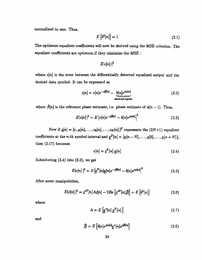
normalized to one. Thus,
E [b2[n]] = 1 (3.1)
The optimum equalizer coefficients will now be derived using the MSE criterion. The
equalizer coefficients are optimum if they minimize the MSE :
where ~ [ n ] is the error between the differentially detected equalized output and the
desired data symbol. It can be expressed as
where &n] is the reference phase estimate, i.e. phase estimate of $[n - 11. Thus,
Now if ~ [ n ] = [c&], . . . , ~ [ n ] , . . . , c ~ [ n ] IT represents the (2N+1) equalizer
coefficients at the n-th symbol interval and yT[n] = - then (2.17) becomes
+I = 3 in1 g[nl
Substituting (3.4) into (3.3), we get
After some manipulation,
EIM I' = f T [ n ] ~ & ] - 2Re [c*' [ n ] ~ ] + E [b2 [n]]
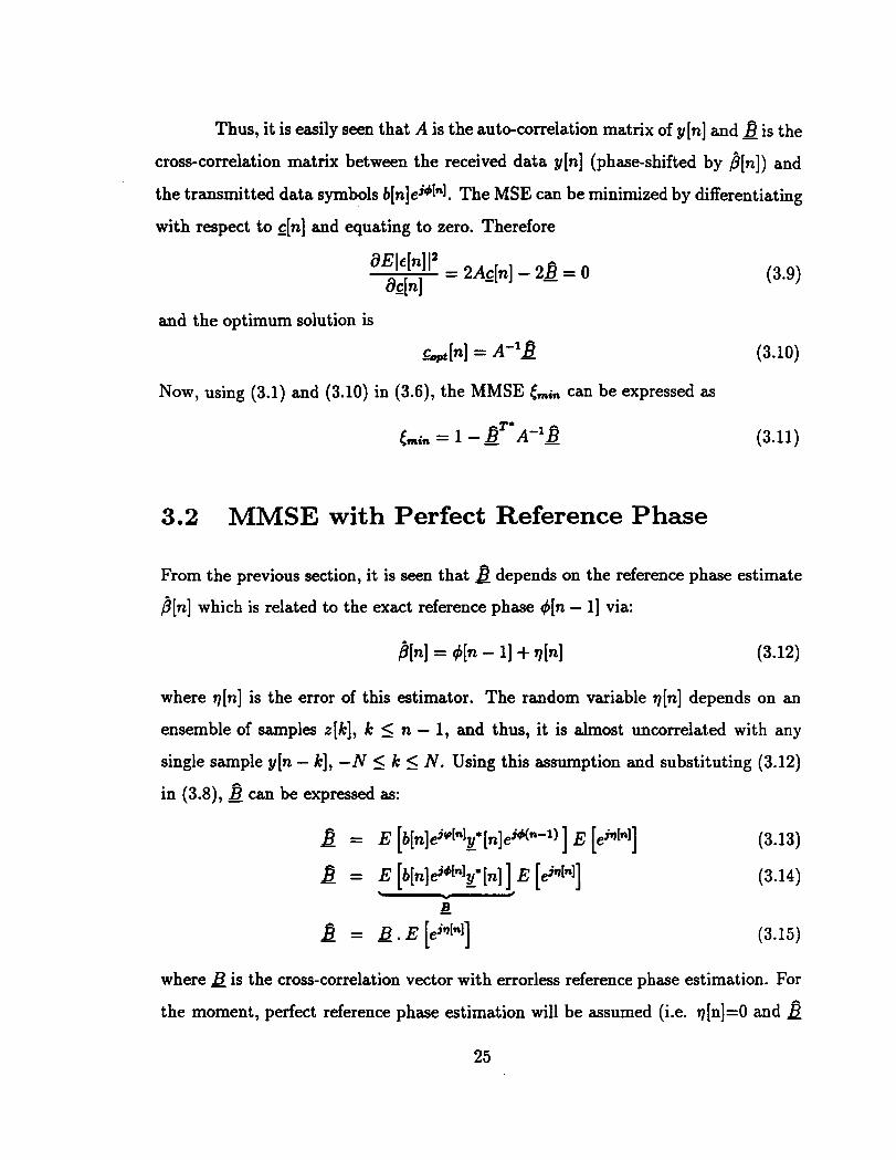
Thus, it is easily seen that A is the auto-correlation matrix of y[n] and is the
cross-correlation matrix between the received data y[n] (phase-shifted by &n]) and
the transmitted data symbols b[n]eji["]. The MSE can be minimized by differentiating
with respect to ~ [ n ] and equating to zero. Therefore
and the optimum solution is
+In] = A-'B
Now, using (3.1) and (3.10) in (3.6), the MMSE tmin can be expressed as
3.2 MMSE with Perfect Reference Phase
From the previous section, it is seen that depends on the reference phase estimate
p[n] which is related to the exact reference phase 4[n - 11 via:
where q[n] is the error of this estimator. The random variable q[n] depends on an
ensemble of samples z[k], k < n - 1, and thus, it is almost uncorrelated with any
single sample y [n - k], - N < k < N. Using this assumption and substituting (3.12)
in (3.8), can be expressed as:
8 = E [b[n] ej*[nl y* [n] ejH"-l) ] E [ej'dnl] - 8 = E [b[n] @["I y* [n] ] E [ejq["1] -
where & is the cross-correlation vector with errorless reference phase estimation. For
the moment, perfect reference phase estimation will be assumed (i.e. q[n]=O and B
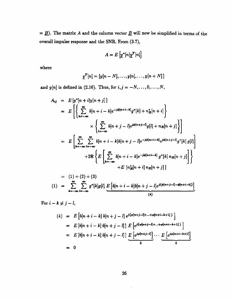
= - B). The matrix A and the column vector B will now be simplified in terms of the
overall impulse response and the SNR. From (3.7),
and y[n] is defined in (2.16). Thus, for i, j = -N, . . . , 0, . . . , N,
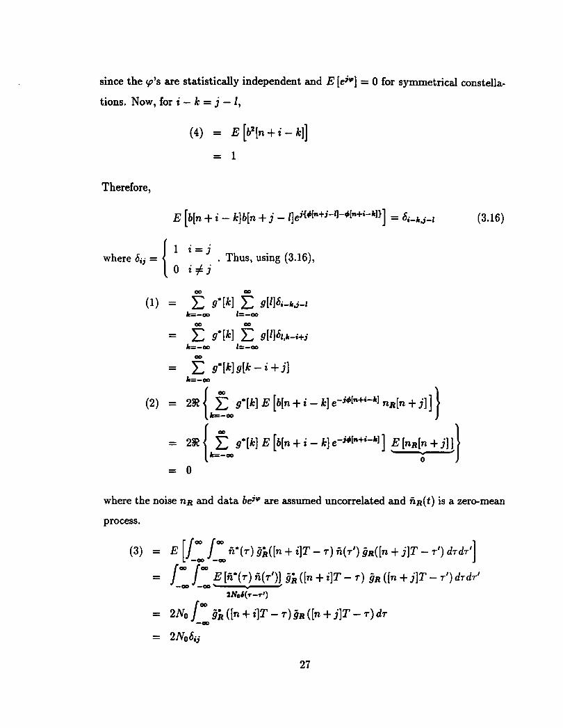
since the p's are statistically independent and E [ejv] = 0 for symmetrical constella-
tions. Now, for i - k = j - I,
( 4 ) = E [b2[n + i - k]] = 1
Therefore,
1 z = j where bij = . Thus, using (3.16),
0 i # j
( 2 ) = 2% C g* [k] E [b[n + i - k] e-j4[n+-k1 n ~ [ n + jl ] { k I W
where the noise nR and data bejv are assumed uncorrelated and fiR(t) is a zero-mean
process.
( 3 ) = E [/OD -QD [", f i * ( + ) &([n + i ] T - T ) fi(rt) aR( [n + j ] T - rt) drdr f ]
- - E [ f i * ( ~ ) G(T')] 3; ( [ n + i ] T - T ) aR ( [ n + j ] T - T I ) drdrl 2N06(r-r')
= 2 ~ 0 1 - & ( [ n + i ] T - r ) h ( [ n + f T - T ) ~ T -OD
since i i ( t ) is white and aR(t) + jR( t ) satisfies Nyquist's first criterion. Therefore, for
i , j = -N,.. . ,o, . . ., N.
The matrix A is Hermitian and positive semi-definite. Now, from (3.14),
where B~ = [B[-N] ,..., B[O] ,... ,BIN]] -
yT[n] = [Y[~-N],...,Y[~I,...,Y~~+N~I - Thus, for i = -N,. . . ,O,. . . , N,
B [i] = E [b[n] ej4in] y [n + i]]
The summation and expectation operators can be interchanged since they are linear.
Therefore,
using (3.16). Therefore, the errorless column vector B is simply a truncated overall
impulse response vector, i.e. B = [g[- N], . . . , g[O], . . . , g[N] 1.
3.3 Reference Phase Error Analysis
In the previous section, perfect reference phase estimation was assumed. However, in
practice, phase estimation errors will occur. In our analysis, perfect receiver decisions
are assumed, and estimation errors are due mainly to channel noise and ISI.
From, Section 3.2, only B depends on ~ [ n ] via (3.15). Therefore, the depen-
dence of fl (and the MMSE) on the reference phase error ~ [ n ] defined in (3.12) wi4
now be found by analyzing E [ e j ~ [ ~ ] ] . From (2. lg),
L Iv [n] I ejfi["] = x z [n - i] exp
i=l
Also, the past equalizer outputs can be expressed by :
where ~ [ n -i] is the equalization error. From [13], for high SNR and with E [b2[n]] = 1,
E [ ~ [ n - i]] = 0 (3.21)
Substituting (3.20) into (3.19), we get
where
and q[n] is the phase estimation error. For q[n] << 1 and E [q[n] ] = 0,
From (3.26), it is seen that q[n] is the phase error of a (real) phasor b[n - i] i=l
L
perturbed by noise ~ [ n - i~e-j&[~-q, and thus the results from [2] can be used. i=1
Thus, we fix b b - I ] , . . . , b[n - L] and calculate the conditional variance of q[n], i.e.
E [q2[n] I b[n - I ] , . . . , b[n - L] 1 . For high SNR and fixed b[n - i] , i = 1,. . . , L, the
asymptotic distribution of q[n] is Tikonov [2] and the conditional probability density
where lo is the modified Bessel function of order zero and A is the SNR of the (real) L L
phasor b[n - i] perturbed by the noise ~ [ n - i]e-jdn-4 which can be expressed i=1 i=l
as:
(2 - il)' A [b[n - 11,. . . , b[n - L]] = i=l
L E [I ~ [ n - ile-jdn-d 1' I b[n - 11,. . . , bin - L]]
i=l (3.29)
-
where the numerator is the power of b[n - i] and the denominator is the variance
L of C ~ [ n - i]e-j4["-4 for fix
i=l expressed as
-
irl
d b[n - i], i = 1,. . . , L. Now, the denominator can be
= xx E [r[n - i]~'[n - k] I b[n - l],.. . ,b[n - L]] x
L = E [~c[n - i] l 2 I b[n - 11,. . ., b[n - L]]
i=l
where we used the fact that the equalization error e[n - i] is practically uncorrelated
with ej4in-4. Therefore, substituting (3.30) into (3.29), we get
{ e b [ n i=l - i][ A [b[n - 11,. . . , b[n - L] ] = (3.31)
E - i] I 2 I b[n - I],.. . , b[n - L]] i=l
and
1 E [r)2[n] I b[n - l],.,b[n- L]] .
A [bin - 11,. . . , b[n - L]]
Therefore,
E [v2[nl] = E
Here we assumed that E [le[n - i] I 2 I b[n - 11,. . . , b[n - L] ] is uncorrelated 2 2
with { t b [ n - i ] ) . For large L, then { k b [ n - i ] ) . L2 {~[b] ) ' . K , where X i=l i=l
3 1
is a constant and thus, it is clear that the assumption is valid. For small L, then
E[le[n - i ] I 2 I b[n - 11,. . . , b[n - L] ] .Y E [le[n - i ] 12] since only a small fraction of
signal samples which are stored in the equalizer are fixed, and thus the equalization
error is almost the same as the one obtained when no signal sample is constrained.
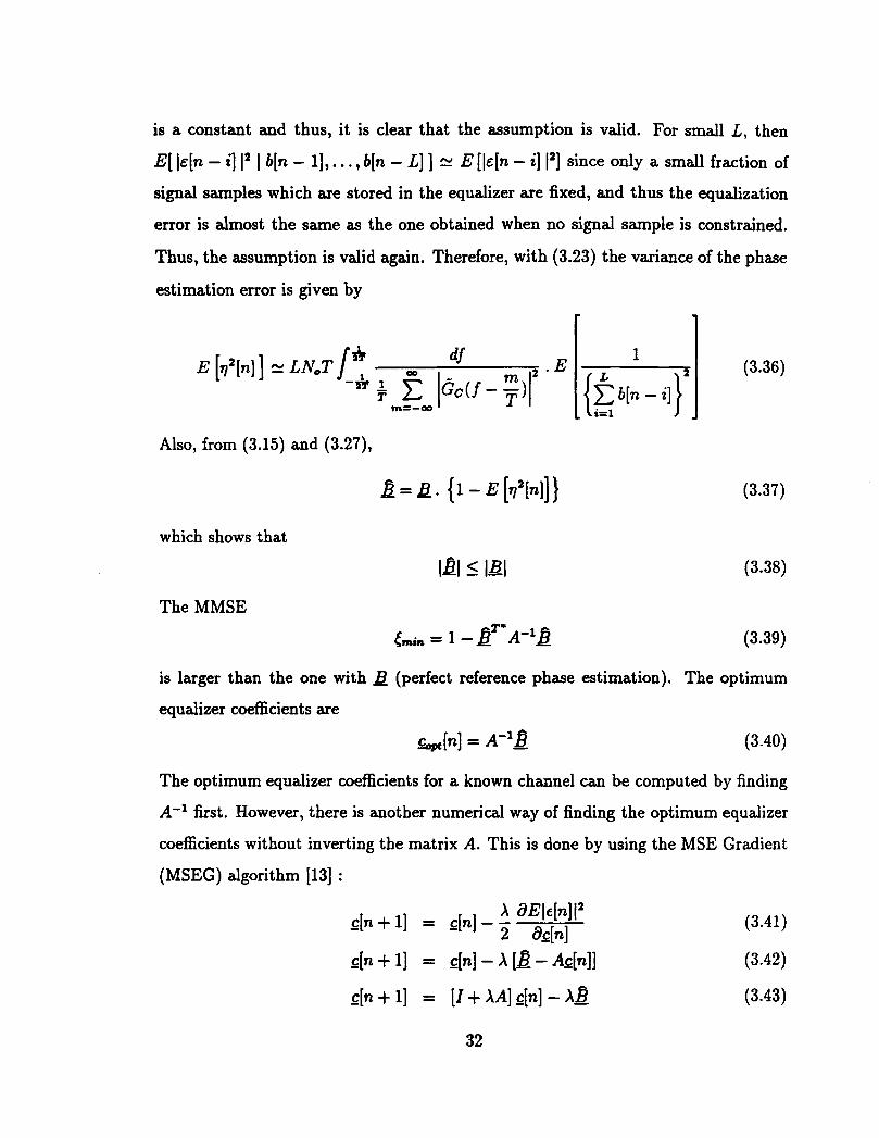
Thus, the assumption is valid again. Therefore, with (3.23) the variance of the phase
estimation error is given by
which shows that
IBI 5 la The MMSE
is larger than the one with (perfect reference phase estimation). The optimum
equalizer coefficients are
c in] = A-~B -opt
The optimum equalizer coefficients for a known channel can be computed by finding
A-' first. However, there is another numerical way of finding the optimum equalizer
coefficients without inverting the matrix A. This is done by using the MSE Gradient
(MSEG) algorithm [13] :
~ [ n + I] = ~ [ n ] - X [B - Ae[n]] (3.42)
c[n + l] = [ I + XA] $n] - A& - (3.43)
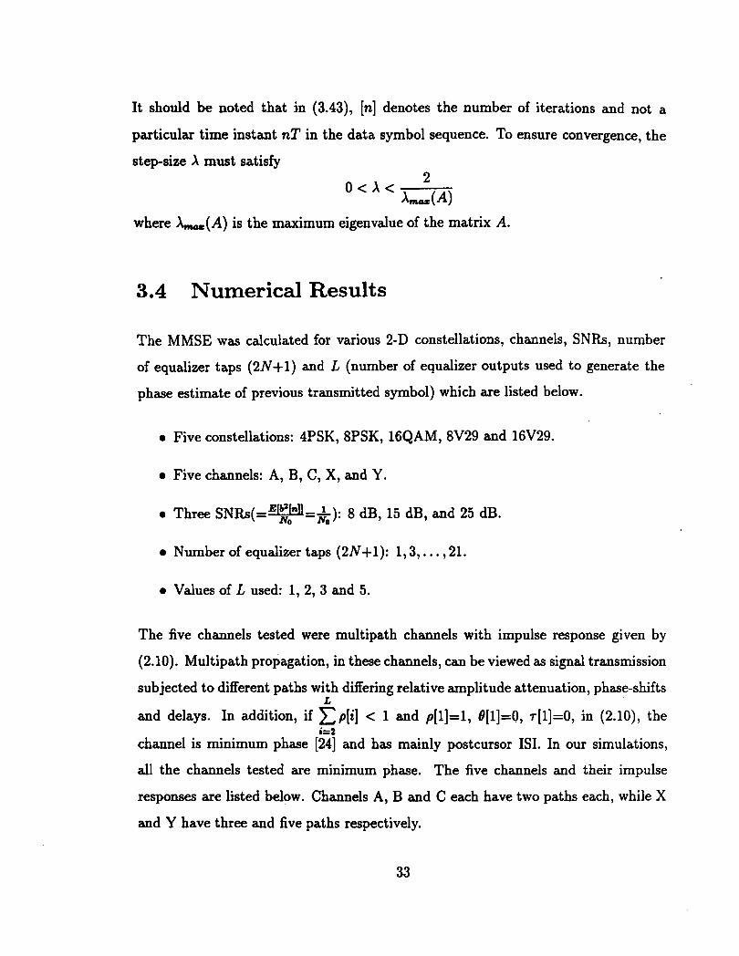
It should be noted that in (3.43), [n] denotes the number of iterations and not a
particular time instant n T in the data symbol sequence. To ensure convergence, the
stepsize X must satisfy
O < A < 2
Ld A)
where X-(A) is the maximum eigenvalue of the matrix A.
3.4 Numerical Results
The MMSE was calculated for various 2-D constellations, channels, SNRs, number
of equalizer taps (2N+1) and L (number of equalizer outputs used to generate the
phase estimate of previous transmitted symbol) which are listed below.
0 Five constellations: 4PSK, 8PSK, lGQAM, 8V29 and 16V29.
0 Five channels: A, B, C, X, and Y.
0 Three S N R ~ ( = ~ = $ - ) : 8 dB, 15 dB, and 25 dB.
Number of equalizer taps (2N+1): 1,3,. . . ,21.
0 Values of L used: 1, 2, 3 and 5.
The five channels tested were multipath channels with impulse response given by
(2.10). Multipath propagation, in these channels, can be viewed as signal transmission
subjected to different paths with differing relative amplitude attenuation, phase-shifts L
and delays. In addition, if p[i] < 1 and p[l]=l, 8[1]=0, ~[1]=0, in (2.10), the i=2
channel is minimum phase (241 and has mainly postcursor ISI. In our simulations,
all the channels tested are minimum phase. The five channels and their impulse
responses are listed below. Channels A, B and C each have two paths each, while X
and Y have three and five paths respectively.
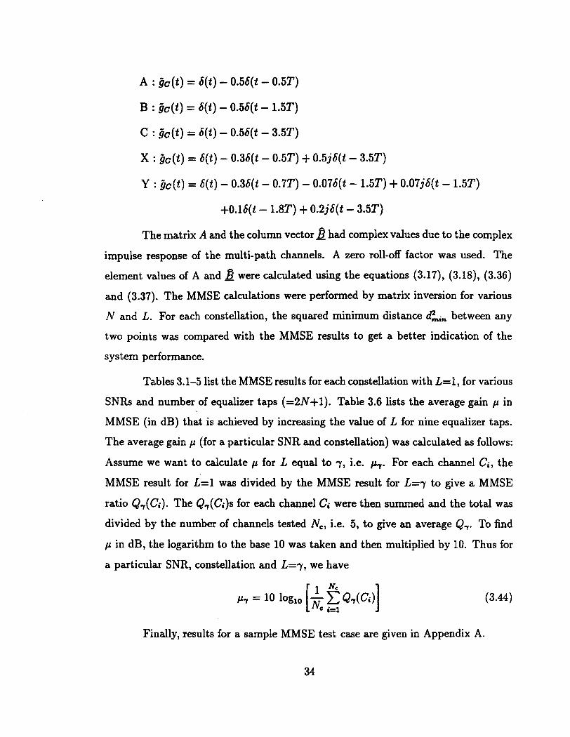
The matrix A and the column vector had complex values due to the complex
impulse response of the multi-path channels. A zero roll-off factor was used. The
element values of A and & were calculated using the equations (3.17), (3.18), (3.36)
and (3.37). The MMSE calculations were performed by matrix inversion for various
N and L. For each constellation, the squared minimum distance &, between any
two points was compared with the MMSE results to get a better indication of the
system performance.
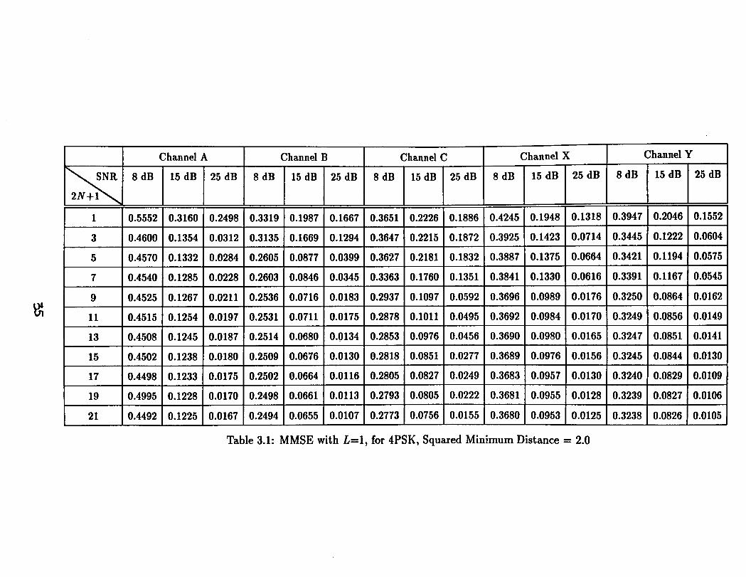
Tables 3.1-5 list the MMSE results for each constellation with L=l, for various
SNRs and number of equalizer taps (=2N+1). Table 3.6 lists the average gain p in
MMSE (in dB) that is achieved by increasing the value of L for nine equalizer taps.
The average gain p (for a articular SNR and constellation) was calculated as follows:
Assume we want to calculate p for L equal to 7, i.e. h. For each channel Ci, the
MMSE result for L=l was divided by the MMSE result for L=7 to give a MMSE
ratio Q,(Ci). The Q,(Ci)s for each channel Ci were then summed and the total was
divided by the number of channels tested N,, i.e. 5, to give an average Q,. To find
p in dB, the logarithm to the base 10 was taken and then multiplied by 10. Thus for
a particular SNR, constellation and L=7, we have
Finally, results for a sample MMSE test case are given in Appendix A.
I I Channel A I Channel B I Channel C I Channel X Channel Y
SNR 8 dB p
Table 3.1: MMSE with L=l, for 4PSK, Squared Minimum Distance = 2.0
Channel A Channel B
8 dB 15 dB 25 dB 8 dB 15dB 25 dB
2N+1
I 1 1 0.5552 1 0.3160 1 0.2498 1 0.3319 1 0.1987 1 0.1667
Channel X Channel Y
8 dB 15 dB 25 dB 8 d B 15 dB 25 dB
0.4245 0.1948 0.1318 0.3947 0.2046 0.1552
0.3925 0.1423 0.0714 0.3445 0.1222 0.0604
0.3887 0.1375 0.0664 0.3421 0.1194 0.0575
- -
Table 3.2: MMSE with L=l, for 8PSK, Squared Minimum Distance = 0.5858
I I Channel A I Channel B I Channel C I Channel X I Channel Y I - - -
SNR 8 dB 15 dB 25 dB 8 dB 15 dB 25 dB 8 d~ 1 5 d ~ 25 d~ 8 dB 15 dB 25 dB 8 d B 15 dB 25dB
1 0.6470 0.3216 0.2499 0.3671 0.2004 0.1667 0.4085 0.2247 0.1886 0.4931 0.1986 0.1318 0.4493 0.2074 0.1552
L I I I I I I I I
Table 3.3: MMSE with L=l , for 8V29, Squared Minimum Distance = 0.7273
I I Channel A I Channel B I Channel C I Channel X I Channel Y I - - - - - - -
SNR 8 dB 15 dB 25 dB 8 dB 15 dB 25 d~ 8 d~ 15 d~ 25 d~ 8 dB 15 dB 25 dB 8 dB 15 dB 25 dB
Table 3.4: MMSE with L=l , for lGQAM, Squared Minimum Distance = 0.4
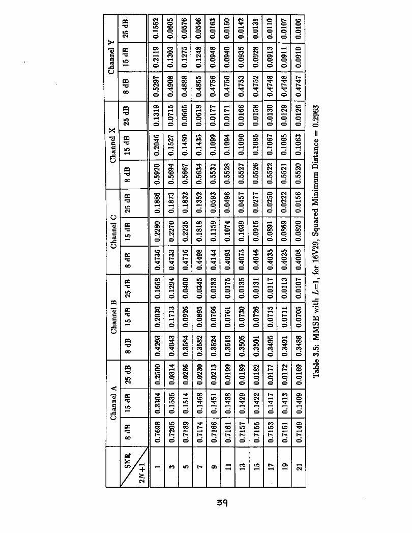
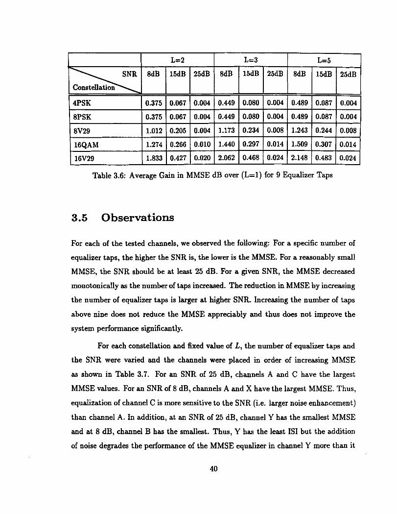
Table 3.6: Average Gain in MMSE dB over (L=l) for 9 Equalizer Taps
3.5 0 bservat ions
For each of the tested channels, we observed the following: For a specific number of
equalizer taps, the higher the SNR is, the lower is the MMSE. For a reasonably small
MMSE, the SNR should be at least 25 dB. For a given SNR, the MMSE decreased
monotonically as the number of taps increased. The reduction in MMSE by increasing
the number of equalizer taps is larger at higher SNR. Increasing the number of taps
above nine does not reduce the MMSE appreciably and thus does not improve the
system performance significantly.
For each constellation and fixed value of L, the number of equalizer taps and
the SNR were varied and the channels were placed in order of increasing MMSE
as shown in Table 3.7. For an SNR of 25 dB, channels A and C have the largest
MMSE values. For an SNR of 8 dB, channels A and X have the largest MMSE. Thus,
equalization of channel C is more sensitive to the SNR (i.e. larger noise enhancement)
than channel A. In addition, at an SNR of 25 dB, channel Y has the smallest MMSE
and at 8 dB, channel B has the smallest. Thus, Y has the least IS1 but the addition
of noise degrades the performance of the MMSE equalizer in channel Y more than it
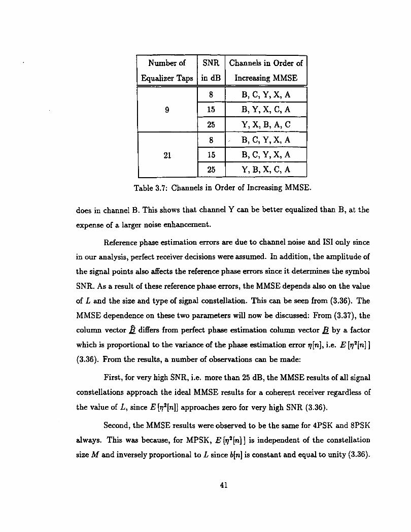
Table 3.7: Channels in Order of Increasing MMSE.
-
Number of
Equalizer Taps
does in channel B. This shows that channel Y can be better equalized than B, at the
expense of a larger noise enhancement.
Reference phase estimation errors are due to channel noise and IS1 only since
in our analysis, perfect receiver decisions were assumed. In addition, the amplitude of
the signal points also affects the reference phase errors since it determines the symbol
SNR. As a result of these reference phase errors, the MMSE depends also on the value
of L and the size and type of signal constellation. This can be seen from (3.36). The
MMSE dependence on these two parameters will now be discussed: From (3.37), the
column vector & differs from perfect phase estimation column vector B by a factor
which is proportional to the variance of the phase estimation error q[n], i.e. E [q2[n] ]
(3.36). From the results, a number of observations can be made:
SNR
in dB
First, for very high SNR, i.e. more than 25 dB, the MMSE results of all signal
constellations approach the ideal MMSE results for a coherent receiver regardless of
the value of L, since E [q2[n]] approaches zero for very high SNR (3.36).
Channels in Order of
Increasing 1 MMSE
Second, the MMSE results were observed to be the same for 4PSK and 8PSK
always. This was because, for MPSK, E [ ~ ~ [ n ] ] is independent of the constellation
size M and inversely proportional to L since b[n] is constant and equal to unity (3.36).
However, although they give the same MMSE results, 4PSK has a smaller probability
of error P, than 8PSK since its minimum distance is larger. Therefore, for the same
P,, the SNR of the 8PSK constellation must be raised to a suitable higher value.
Third, 16V29, 16QAM and 8V29 gave larger MMSE results than MPSK.
Thus, constellations with signal points of varying amplitudes have degradations in
performance, i.e. larger MMSE results, compared to constant amplitude signal con-
stellations. In addition, the l6V29 constellation gave larger MMSE results than both
16QAM and 8V29, since it has signal points with smallest amplitudes. Therefore, con-
stellations with smaller amplitude signal points have larger degradations in MMSE
performance.
Using a larger L, the constellations with smaller amplitude symbol points had
larger MMSE performance gains, i.e. larger reductions in MMSE. Thus, by increasing
L, 16V29, 16QAM, 8V29 and MPSK had performance gains which decreased in that
order. As a result, using a larger L reduces the difference in MMSE performance
between the V29, QAM, and PSK constellations. Furthermore, by increasing L, the
system performance approaches that of combined coherent detection and equalization.
In addition, the gain in MMSE(dB), i.e. p , by using a value of L larger than one, was
very significant, especially for low SNR. Also, using L=3 or L=5 gives appreciable
gains in performance over L=2. However, larger values of L do not yield appreciable
performance gains over L=3. Therefore, three appears to be the best value for L.
This is because increasing L increases the SNR of the reference signal from which the
phase reference is extracted until it approaches coherent PSK. It appears that the
reference phase SNR of the differential detected signal sufficiently approaches that of
a coherently detected signal at L=3.
Finally, the difference in MMSE between coherent and differentially coherent
detection is smaller here than in [20]. This is due to the way that the reference phase
is derived in this work. In [20], an adaptive equalizer was used for differentially co-
herent reception and the MMSE obtained was about 3 dB more than that obtained
in the coherent case. One previous equalizer output was used to generate the refer-
ence estimate and its conjugate was used in the decision variable, together with the
equalizer output. Thus, errors in the reference estimate caused both ampli tude and
phase errors in the receiver's decisions. In our case, the improved phase reference
estimate &n], (which can be generated by using more than one past equalizer output
to smooth channel noise), is used only to phase-shift the current equalizer output.
In other words, we process the reference sample by a limiter which removes the am-
plitude noise. Thus, our reference estimate causes on ly phase errors in the receiver's
decisions and therefore, the difference in MMSE between coherent detection and dif-
ferential detection is less than 3 dB in our case. In addition, increasing L allows
the system performance to approach that of combined coherent detection and linear
equalization. As a result, our proposed receiver has better system performance which
approaches that of combined coherent detection and linear equalization.
Chapter 4
Adaptive Equalization for
Unknown Channels
The combination of decision-feedback differentially coherent detection with adaptive
equalization is considered in this chapter. In Section 4.1, the conventional Least-
Mean-Square (LMS) adaptive algorithm and some fast-converging algorithms, e.g.
Kalman are briefly reviewed. Following this, the LMS algorithm, which is used for
adapting the linear equalizer, is described. Simulation results (for a specific number
of equalizer taps, SNR and L) and graphs which compare average convergence rates
and residual MSEs for different test cases (i.e. different constellations, channels and
step-sizes.), are presented in Section 4.2. Finally, these results are discussed in Section
4.3.
4.1 The LMS Adaptive Equalizer
For many practical wireless systems, the channel characteristics are usually not known
beforehand, and therefore the equalizer must adapt to the unknown channel. In
addition, the characteristics of these channels may vary sufficiently with time so that
adaptive equalization is also necessary during normal data transmission.
A comprehensive survey on the early days of adaptive equalization can be
found in [17]. In 1960, Widrow and Hoff [14] presented the Least-Mean-Squares
(LMS) error adaptive filtering scheme which has been used extensively in the last
three decades. In addition, key papers [27] and [28] have contributed to the under-
standing of the convergence of the LMS stochastic update algorithm for transversal
equalizers, including the effect of channel characteristics (eigenvalue spread of the
auto-correlation matrix) and the number of equalizer taps on the rate of convergence.
First, in [27], the assumption of statistical independence for the random equalizer
input vectors - y[n] (from one instant [n] to another instant [n+l]), which direct equal-
izer convergence, was investigated and it was found that although this assumption is
far from true, the results obtained using this assumption are in excellent agreement
with the actual performance of the LMS equalizer convergence.
In [28], Ungerboeck considered the MSE criterion instead of the expected
tap-gain errors relative to their optimum values (considered by Gersho in [21]). In
addition, he assumed the equalizer input vectors - y[n] at successive instants to be
statistically independent and showed that the influence of the number of equalizer
taps, and not only the channel characteristics, dominates the speed of convergence.
This was opposed to (211, where the speed of convergence (for Gersho's criterion,
i.e. the expected tap-gain errors relative to their optimum values) was shown to
depend only on the channel characteristics. As a result, Ungerboeck suggested a new
criterion for stability, which imposed a much narrower upper bound on the step-size
than the one found in [21] and a corresponding optimum initial step-size parameter
for LMS adaptive equalization. Finally, he showed the MSE convergence is faster
in practice than theoretically predicted and suggested that step-sizes slightly less
than the optimum step-size should be chosen, since the assumption of statistical
independence of the equalizer input vectors - y[n] at successive instants is not true in
practice.
In our simulations, the LMS algorithm is used to adapt the linear equalizer to
the channel because of its simplicity and robustness. However, its main drawback is its
slow convergence compared with the more sophisticated algorithms [23]-[25]. In [23],
the Kalman filtering algorithm was described. It can be used to estimate the equalizer
coefficients vector at each symbol interval and its convergence rate was shown to be
proportional to the number of equalizer taps and independent of the eigenvalue spread.
However, it requires on the order of N2 operations per iteration for an equalizer
with N taps. In [24], a self-orthogonalizing algorithm was compared to the Kalman
algorithm of [23] and the LMS algorithm. The algorithm tries to accelerate the rate
of convergence by reducing the eigenvalue spread of the channel-correlation matrix,
i.e. by making the eigenvalues equal, since a large eigenvalue spread slows the rate
of convergence. It was found that the proposed self-orthogonalizing algorithm, which
was less complex than the Kalman, converged much faster than the LMS algorithm
but was slower than the Kalman algorithm. The Kalman algorithm of [23] was later
recognized as a form of a Recursive-Least-Squares (RLS) algorithm and the idea of
fast Kalman filtering was introduced [25]. This algorithm took advantage of the
data structure by using the "shifting property" of RLS algorithms and reduced its
computational complexity to an order of N operations per iteration for an equalizer
with N taps. Therefore, the algorithm performs as well as the one in (231 while
avoiding its computational complexity.
The LMS algorithm will now be discussed. It is similar to the MSEG al-
gorithm (3.41) but uses an instant squared error instead of the mean squared error
because the ensemble averages represented by the matrix A and $ are not known in
practice. The LMS algorithm is also referred to in the literature as the stochastic
gradient (SG) algorithm [13]. Using the LMS algorithm, the filter coefficient vector
is updated by
where e[n] is the error at the n-th iteration, [n] denotes a particular symbol interval
(or time instant t=nT), g[n] = [ ~ - ~ [ n ] , . . . , ~ [ n ] , . . . ,cN[n]] and X is the step-size.
Using (3.2), the error is given by:
where Bin] is the reference phase estimate. Differentiating the instant squared error
1~[n]1~ with respect to ~ [ n ] , we get :
where t[n] = ~ ~ [ n ] ~ [ n ] . Therefore, substituting (4.2) in (4.1), we get :
Thus, each equalizer tap q[n] is updated using the error ~ [ n ] , the phase
reference estimate &n] and the received sample y[n + k] for k = -N, . . . ,O, . . . , N.
The algorithm of (4.4) will now be explained referring to Figure 2.4. The
equalizer adaptation is driven by the error signal ~ [n ] , which indicates to the equalizer
in which direction the coefficients ~ [ n ] must be changed to reduce the squared error
Ie[n] 1'. Specifically, the input sample to the equalizer, y [n - k] is taken from the output
of the same unit delay and is used for multiplication by ck[n]. The resulting product
contributes to the summation for z[n], which is then phase-shifted by B[n] and the
data symbol b[n]ej~["] is subtracted from it to give the error ~ [ n ] . The increment of
the tap coefficient ck[n] is -Xc[n]y*[n - k]ejbM, where yk[n - k] is phase-shifted by
&I] to compensate for the unknown rotation of these samples.
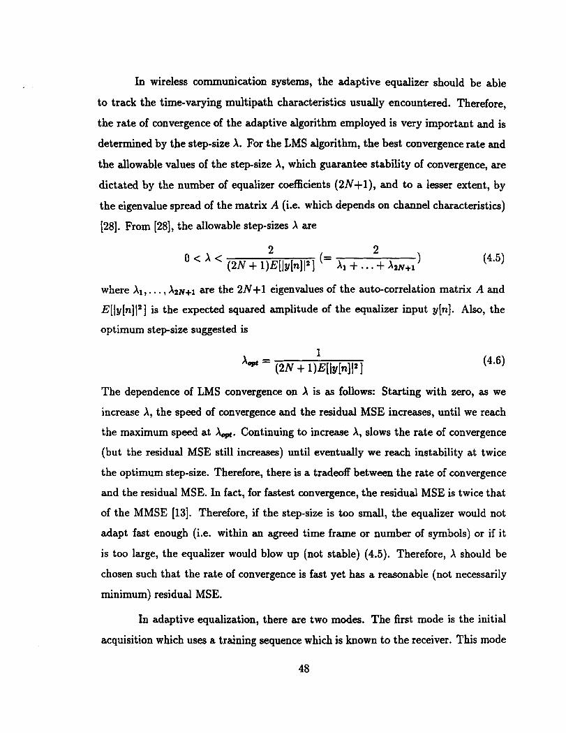
In wireless communication systems, the adaptive equalizer should be able
to track the time-varying multipath characteristics usually encountered. Therefore,
the rate of convergence of the adaptive algorithm employed is very important and is
determined by the stepsize A. For the LMS algorithm, the best convergence rate and
the allowable values of the step-size A, which guarantee stability of convergence, are
dictated by the number of equalizer coefficients (2N+1), and to a lesser extent, by
the eigenvalue spread of the matrix A (i.e. which depends on channel characteristics)
[28]. From [28], the allowable step-sizes A are
where Al, . . . , AzN+l are the 2N+1 eigenvalues of the auto-correlation matrix A and
E[ly[n] 12] is the expected squared amplitude of the equalizer input y[n]. Also, the
optimum step-size suggested is
The dependence of LMS convergence on A is as follows: Starting with zero, as we
increase A, the speed of convergence and the residual MSE increases, until we reach
the maximum speed at A#. Continuing to increase A, slows the rate of convergence
(but the residual MSE still increases) until eventually we reach instability at twice
the optimum step-size. Therefore, there is a tradeoff between the rate of convergence
and the residual MSE. In fact, for fastest convergence, the residual MSE is twice that
of the MMSE [13]. Therefore, if the step-size is too small, the equalizer would not
adapt fast enough (i.e. within an agreed time frame or number of symbols) or if it
is too large, the equalizer would blow up (not stable) (4.5). Therefore, A should be
chosen such that the rate of convergence is fast yet has a reasonable (not necessarily
minimum) residual MSE.
In adaptive equalization, there are two modes. The first mode is the initial
acquisition which uses a training sequence which is known to the receiver. This mode
is used to initially adapt the equalizer to the channel and, thus uses actual data
bejv to generate the error signal. Once the equalizer converges in an specific period of
time, the second mode of adaptive equalization can begin. In the second mode, actual
receiver decisions are substituted for the known training sequence and normal data
transmission occurs. This mode of equalizer adaptation is called the decision-directed
mode since receiver decisions kj* are used to generate the error e[n], and the phase
estimate bin) This is seen from Figure 2.4 and equalizer adaptation takes place in a
decision-feedback manner. However, this mode of equalizer adaptation cannot track
fast variations in the channel characteristics. As a result, it may be necessary to use
the first mode to re-adapt the equalizer to the channel.
The adaptive MSE (AMSE) simulation results using the LMS adaptive algo-
rithm for different test cases will now be discussed.
4.2 Simulation Results
Simulations of the equalizer adaptation were performed using the LMS algorithm.
Three parameters of the simulations were kept constant:
0 Nine (=2N+1) equalizer taps were used. Using a larger number of taps in-
creases the delay in the equalizer and does not result in any substantial gain in
performance, with the channels that were tested in this work.
Three equalizer samples used to generate the improved reference phase estimate
(i.e. L was chosen to be 3) since the gain in performance over L=2 is substan-
tial and because using any larger value of L e.g. L=5 does not result in an
appreciable gain in performance.
The SNR was set to 25 dB. A lower SNR would require a prohibitive large
number of simulations.
The three other parameters in the simulations form the basis for different test
cases. These parameters are the signal constellation, the channel and the step-size A.
The choices for each were as follows:
Four constellations: 8PSK, 8V29, 16QAM and 16V29.
Two channels: A and X.
Step-sizes: 0.0005, 0.001, 0.002, 0.005, 0.01, 0.02, 0.05 and 0.1. For our nine
tap equalizer and with E[ly[n]12] 1, Ungerboeck's optimal step-size is 0.1.
Results were examined and the two step-sizes A=0.005 and X=0.05 were chosen
for presentation since they best summarize the trade-offs in selecting the step
size.
For the LMS simulations, training sequences were used, i.e. perfect receiver
decisions were assumed. Each sequence had a length of 3220 data symbols to en-
sure that steady-state convergence had been achieved. All nine equalizer taps were
initialized to zero for each trial.
Initially, in our simulations, twenty independent trials were performed for
each test case (i.e. choice of constellation, channel and step-size) and an average
learning curve was calculated. However, the average learning curves were very noisy
due to an insufficient number of trials. At an SNR of 25 dB, it was found that we
need approximately sixty trials to get reasonable smooth average learning curves. All
simulation results were then examined and are summarized by eight graphs and two
tables, shown on the next few pages.
The first four graphs, i.e. Figures 4.1-4, were each derived for a separate
test case (i.e. either 8PSK or 16QAM used in either channel A or X, using X equal
to 0.005). Each graph plots the squared error versus the number of iterations and
compares sixty trial runs with an average learning curve. It is seen that the number
Squared Error
'Channel A, S t e p = 0.005' - 'Channel At S t e p = 0.05 ' --. ' Channel X, S t e p = 0.005' - - - 'Channel X, S t e p = 0 .05 ' -- - - - .
500 1000 1500 2000 2500 3000 Number of I t e r a t i o n s
Figure 4.5: Average Learning Curves for 8PSK.
) . . . . . I . . . . . .
0 500 1000 1500 2000 2500 3000 Number of Iterations
Figure 4.7: Average Learning Curves for 16QAM.
r l r l r l r l Q, Q, Q, Q, C C C C C C C C t % t % Q I C C C C UUUU ....
1 I Channel A I Channel X I Step-Size 0.005 0.05 0.005 0.05
Constellation I
Table 4.1: Comparison of Residual MSEs and MMSEs for 25 dB
of independent trials, i.e. 60, used to calculate the curves was sufficient since the
dispersion is reasonable.
Consequently, the last four graphs, i.e. Figures 4.5-8, compare the average
learning curves of different test cases. Each graph corresponds to a particular con-
stellation, and compares four different test cases (i.e. either X=0.005 or A=0.05 used
in either channel A or X). Finally, each graph plots the logarithm of the MSE versus
the number of iterations so that differences in convergence behaviour between the
different test cases can be noticed more easily.
Table 4.1 compares the residual MSEs obtained from Figures 4.5-8 with the
calculated MMSE results of Section 3.4. In order to compare the constellations from
a probability of error point of view, we used the squared minimum Euclidean distance
normalised to the number of bits per symbol, log, M, and the residual MSE, [. This quantity in [dB] is given by:
Although, a may not give an accurate indication to the actual probability of error
P. I( exp [d?,, y] which can be arrived at since P. is proportional to the
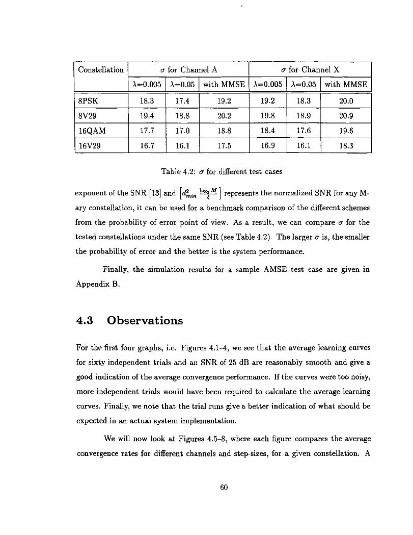
Table 4.2: a for different test cases
a for Channel X Constellation
8PSK
8V29
l6QAM
16V29
lo M exponent of the SNR [13] and [b,;, +] represents the normalized SNR for any M-
ary constellation, it can be used for a benchmark comparison of the different schemes
from the probability of error point of view. As a result, we can compare a for the
tested constellations under the same SNR (see Table 4.2). The larger a is, the smaller
the probability of error and the better is the system performance.
a for Channel A
Finally, the simulation results for a sample AMSE test case are given in
Appendix B.
4.3 Observations
For the first four graphs, i.e. Figures 4.1-4, we see that the average learning curves
for sixty independent trials and an SNR of 25 dB are reasonably smooth and give a
good indication of the average convergence performance. If the curves were too noisy,
more independent trials would have been required to calculate the average learning
curves. Finally, we note that the trial runs give a better indication of what should be
expected in an actual system implementation.
X=0.005
19.2
19.8
18.4
16.9
with MMSE
19.2
20.2
18.8
17.5
X=0.005
18.3
19.4
17.7
16.7
We will now look at Figures 4.5-8, where each figure compares the average
convergence rates for different channels and step-sizes, for a given constellation. A
X=0.05
17.4
18.8
17.0
16.1
X=0.05
18.3
18.9
17.6
16.1
with MMSE
20.0
20.9
19.6
18.3
MSE convergence cutoff point of 0.05 was chosen since the average learning curves
passed through this level only once before settling down to the residual MSE levels
between 0.02 and 0.035. Thus, the average learning curves for different channels and
step-sizes were compared for each graph, using this MSE cutoff level of 0.05. The
following was observed:
For channel A, the k 0 . 0 5 step-size converged after approximately 125 sym-
bols and the k 0 . 0 0 5 step-size converged after about 1000 symbols. For channel X,
the k 0 . 0 5 step-size converged after approximately 100 symbols and the A=0.005
step-size converged after about 750 symbols. Thus, for a given A, the rate of conver-
gence is faster for channel X than for channel A. In addition, the rate of convergence
for the k 0 . 0 5 is faster than for k0.005.
Table 4.1 shows that the residual MSEs approach but never reach the MMSE
results calculated in Section 3.4. This is due to the equalizer coefficients which are
never exactly optimum. For a given A, Table 4.1 shows that the residual MSE is
smaller for channel X than for channel A. Also, for a given channel, the residual MSE
is larger for b 0 . 0 5 than for k0.005. In addition, it was found that the X=0.05
and A=0.005 step-sizes have average residual MSEs of 50% and 25% excess MSEs
respectively, where excess MSE is the MSE over and above the MMSE possible. As a
result, this shows that the larger the step-size A , the larger the excess MSE, since the
equalizer coefficients have a larger variance about the optimum values. For X=0.05,
we see that the proposed receiver adapts very quickly to unknown channels while
giving a residual MSE which is only a small percentage larger than that of X=0.005.
Thus, A=0.05 seems to be a better choice.
In addition, the speed and stability of the MSE convergence were compared
for the tested constellations. Close examination of the last four graphs and Table 4.1
shows that 16V29 converges slightly faster and has a slightly smaller residual MSE
than 16QAM (which is more noticeable in channel A). However, from Table 4.2,
16QAM has a smaller probability of error due to its larger minimum distance dm;,.
Also, 8PSK is better than 8V29 in terms of both convergence speed and residual
MSE which was more noticeable in channel X than in channel A. Nevertheless, the
minimum distance dmin of 8V29 is larger than that of 8PSK, and from Table 4.2, we
have that 8V29 has a smaller probability of error than 8PSK, especially for channels
with severe IS1 e.g. channel A.
Finally, Table 4.2 compares a for the tested constellations and shows that
a decreases (the probability of error increases) for 8V29, 8PSK, 16QAM, 16V29, in
that order, for the tested channels. In addition, Table 4.2 allows us to calculate the
increase in SNR necessary to achieve the same a. On the average, for k0.005, the
SNR must be increased by 0.7 and 1.0 dB for channels A and X respectively, to achieve
the a associated with the MMSE. Also, for k 0 . 0 5 , the SNR must be increased by
an average of about 0.9 dB and 1.1 dB for channels A and X respectively, to achieve
the same a as the X=0.005 case.
Chapter 5
Conclusions
A combined linear equalization and decision-feedback differentially coherent detection
structure for indoor wireless communication channels was proposed. These channels
were modeled as multipath channels since multipath propagation is one of the major
impairments in wireless communication systems. In these channels, carrier phase
tracking is difficult and differentially coherent reception is attractive since it does
not require phase-tracking. However, there is a loss in performance compared to
coherent detection that approaches 3 dB for MPSK(M>2). Therefore, an improved
technique based on decision-feedback differentially coherent detection was used whose
performance approaches that of coherent detection. In addition, this differentially
coherent scheme can be combined quite easily with known equalization techniques.
This is necessary since IS1 due to multipath is a major problem in these channels.
In this work, the integration of decision-feedback differential detection with linear
equalization has been considered. In addition, two-dimensional signal constellations
were considered, in the hope of achieving a high data transmission rate, in a given
bandwidth.
The MSE criterion was used and MMSE results were calculated for known
channels, taking into account reference phase estimation errors. It was seen that
the MMSE performance degrades for 16V29, 16QAM, 8V29 and 8PSK in decreasing
order, since constellations with signal points of smaller amplitude have a larger degra-
dation. However, using a larger value of L, i.e. number of equalizer outputs used to
generate the reference phase, reduces the degradation in MMSE performance, since
constellations with smaller amplitude signal points gain more in MMSE performance.
Thus, the performance of the V29 and QAM signal constellations approach that of the
PSK signal constellation and a high data transmission rate can be achieved in a given
bandwidth. Furthermore, increasing L allows the system performance to approach
that of combined coherent detection and equalization.
In an adaptive mode, the LMS algorithm was used. The simulations were
performed with a 9 tap equalizer, L=3 and an SNR of 25 dB since for known channels,
these values were found to be to be sufficient for a reasonably small MMSE. Using
a MSE cutoff level of 0.05, the equalizer converges within 125 iterations and has
a residual MSE of about 0.029 (50% excess MSE) for A=0.05. For A=0.005, the
equalizer converges within 1000 iterations with a residual MSE of 0.024 (25% excess
MSE). Therefore, k0 .05 seems to be the better choice. In addition, 8PSK (16V29)
converges slightly faster and has a slightly smaller residual MSE than 8V29 (16QAM).
However, the difference in MSE convergence performance for the tested constellations
is almost negligible for L=3. Finally, at the same Eb, the constellations 8V29, 8PSK,
16QAM and 16V29 have probabilities of error in increasing order.
For a sufficiently large L, e.g. L=3, the combination of the decision-feedback
differentially coherent detection structure with linear equalization performs as well as
combined coherent detection and linear equalization, with the advantage that it can
be used when carrier phase tracking is difficult e.g. fading multipath channels, burst
cornrnunicat ion. In addition, the receiver shows very small MMSE differences be-
tween different two-dimensional constellations. Over practical wireless channels, the
proposed receiver seems to have significant advantages with respect to conventional
coherent receivers and we will now suggest further work in this area of combining
equalization with differentially coherent detection.
Suggestions for Further Work
To simplify the analysis, receiver decisions were assumed error-free with high SNR
and actual information phases cp[n - k] for k = 1,. . . , L - 1 were used in the equalizer
adaptation simulations. Therefore, it would be of interest to analyze the effects of
decision errors on the adaptation process and on the residual MSE as well. In addition,
simulations should also be performed for non-zero excess-bandwidth pulses.
To improve performance, one can use decision-feedback equalizers (DFEs)
with the decision-feedback differentially coherent detection structure of [2]. The DFE
cancels the dominant postcursor IS1 in minimum phase multipath channels without
noise enhancement. Therefore, this combination is worth further investigation.
Improving the reference phase estimation for the QAM and V29 constella-
tions may improve results. Therefore, reference phase estimation which is optimized
for amplitude and phase signal constellations should be used in conjuncture with dif-
ferential detection. Also, the reference phase estimation for non-stationary channels
can be improved by introducing a forgetting factor. Therefore, past equalizer outputs
can be weighted such that the more recent equalizer outputs will have more influence
on the reference phase estimate, thus improving the phase tracking capabilities.
Finally, the adaptive equalizer should be tested using faster adaptation algo-
rithms e.g. fast Kalman algorithm [25].
Bibliography
[I] G. D. Forney Jr., R. G. Gallager, G. R. Lang, F. M. Longstaff, and S. U. Qureshi,
"Efficient modulation for band-limited channels," IEEE J. Sel. Areas Commun.,
vol. SAC-2, no. 5, pp. 632-647, Sep. 1984.
[2] H. Leib and S. Pasupathy, "The phase of a vector perturbed by Gaussian noise
and differentially coherent receivers," IEEE Trans. Info. Theory, vol. 34, no. 6,
pp. 1491-1501, Nov. 1988.
(31 S. G. Wilson, J. Freebersyser, and C. Marshall, "Multisymbol detection of
DPSK," GLOBECOM, Dallas, Texas, pp. 1692-1697, Nov. 27-30, 1989.
[4] D. Divsalar and M. K. Simon, "Differential detection of MPSK," IEEE Trans.
Commun., vol. COM-38, no. 3, pp. 300-308, Mar. 1990.
[5] H. Leib and S. Pasupathy, "Noncoherent block demodulation of PSK," IEEE
Vehicular Technology Conf., Orlando, Florida, pp. 407-411, May 6-9, 1990.
[6] C. R. Cahn, "Combined digital phase and amplitude modulation communication
systems," IRE Trans. Commun., vol.CS-8, no. 3, pp. 150-154, Sep. 1960.
[7] J. C. Hancock and R. W. Lucky, "Performance of combined amplitude and phase-
modulated communications systems," IRE Trans. Commun., vol. CS-8, no. 4,
pp. 232-237, Dec. 1960.
[8] C. N. Campopiano and B. G. Glazer, "A coherent digital amplitude and phase-
modulation scheme," IRE Trans. Commun., vol. CS-10, no. 1, pp. 90-95, Mar.
1962.
[9] G. J. Foschini, R. D. Gitlin, and S. B. Weinstein, "On the selection of a two-
dimensional signal constellation in the presence of phase jitter and Gaussian
noise," Bell Sys. Tech. J., vol. 52, no. 6, pp. 927-965, Ju1.-Aug. 1973.
[lo] G. J. Foschini, R. D. Gitlin, and S. B. Weinstein, "Optimization of two-
dimensional signal constellations in the presence of Gaussian noise," IEEE Trans.
Commun., vol. COM-22, no. 1, pp. 28-37, Jan. 1974.
[ll] C. M. Thomas, M. Y. Weidner, and S. H. Durrani, "Digital amplitude phase
keying with M-ary alphabets," IEEE Trans. Commun., vol. COM-22, no. 2, pp.
168-180, Feb. 1974.
[12] D. N. Godard, "Self-recovering equalization and carrier tracking in two- dimen-
sional data communication systems," IEEE Trans. Commun., vol. COM-28, no.
11, pp. 1867-1875, Nov. 1980.
[13] E. A. Lee and D. G. Messerschmitt, Digital Communications. Boston: Kluwer
Academic Publishers, 1988.
[14] B. Widrow and M. E. Hoff Jr., "Adaptive switching circuits," IRE Wescon Conv.
Rec., Pt. 4, pp. 96-104, Aug. 1960.
[15] R. D. Gitlin, E. Y. Ho, and J. E. Mazo, "Passband equalization of differentially
phase-modulated data signals," Bell Sys. Tech. J., vol. 52, no. 2, pp. 219-238,
Feb. 1973.
[16] J. G. Proakis, Digital Communications. New York: McGraw-Hill, 1983.
[17] R. W. Lucky, "A survey of the communication theory literature: 1968-1973,"
IEEE Trans. Info. Theory, vol. IT-19, no. 5, pp. 725-739, Nov. 1973.
[18] R. D. Gitlin and K. H. Mueller, "Optimization of digital postdetection filters for
PSK differential detectors," IEEE Trans. Commun., vol. COM-24, no. 9, pp.
963-970, Sep. 1976.
[19] B. Farhang-Boroujeny, and L. F. Turner, "An intersymbol interference cancella-
tion equaliser for use in systems employing envelope detection," IEE Proc., Pt.
F, Commun. Radar Signal Process., vol. 127, no. 6, pp. 485496, Dec. 1980.
[20] P. Sehier and G. Kawas Kaleh, "Adaptive equaliser for differentially coherent
receiver," IEE Proc., Pt. I, Commun. Speech Vision, vol. 137, no. 1, pp. 9-12,
Feb. 1990.
[21] A. Gersho, "Adaptive equalization of highly dispersive channels," Bell Sys. Tech.
J., vol. 48, no. 1, pp. 55-70, Jan. 1969.
(221 S. U. H. Qureshi, "Adaptive equalization," IEEE Proc., vol. 73, no. 9, pp. 1349-
1387, Sep. 1985.
[23] D. N. Godard, "Channel equalization using a Kalman filter for fast data trans-
mission," IBM J. Res. Develop., vol. 18, no. 3, pp. 267-273, May 1974.
[24] R. D. Gitlin and F. R. Magee, "Self-orthogonalizing adaptive equalization algo-
rithms," IEEE Trans. Commun., vol. COM-25, no. 7, pp. 666-672, July 1977.
I251 D. D. Falconer and L. Ljung, "Application of fast Kalman estimation to adaptive
equalization," IEEE Trans. Commun., vol. COM-26, no. 10, pp. 1439-1446, Oct.
1978.
[26] H. Sari, S. Moridi, L. Desperben, and P. Vandamme, "Baseband equalization and
carrier recovery in digital radio systems," IEEE Trans. Commun., vol. COM-35,
no. 3, pp. 319-327, Mar. 1987.
(271 J. E. Mazo, "On the independence theory of equalizer convergence," Bell Sys.
Tech. J., vol. 58, no. 5, pp. 963-993, May-Jun. 1979.
(281 G . Ungerboeck, "Theory on the speed of convergence in adaptive equalizers for
digital communications," IBM J. Res. Develop., vol. 16, no. 6, pp. 546-555, Nov.
1972.
[29] W. H. Press, B. P. Flannery, S. A. Teukolsky, and W. T. Vetterling, Numerical
Recipes in C, The Art of Scientific Computing. Cambridge University Press,
1988.
Appendix A
A.l Program Overview
The computer program was written using the C programming language and ran under the SUN 0s. The program consists of seven separate files. Data was read from a specified input file and all results were written to a specified output file. In addition, two other output files were created for ease of plotting the LMS simulation results. One file stored trial results and the other stored the average learning curves, i.e. average results of 60 trials.
Input File Data
Test constellation: PSK, QAM, V29 and any other format.
Multipath channel Parameters: Number of paths-1, amplitude attenuations, phase- shifts and relative delays
Roll-off factor of overall desired response. Any number from 0 to 1.
0 Step-sizes to be used in LMS simulations.
Noise Power in dB.
Number of Equalizer Taps besides the reference tap: called N, i.e. min.,max.,step.
Number of Equalizer Outputs for phase estimate: L, i.e. min.,max.,step.
0 The output data filenames.
Program Files and Functions
The seven files and their functions are as follows:
EQ.C: Main program file. Reads input file and generates output files. Calls MMSE.C and AMSE.C.
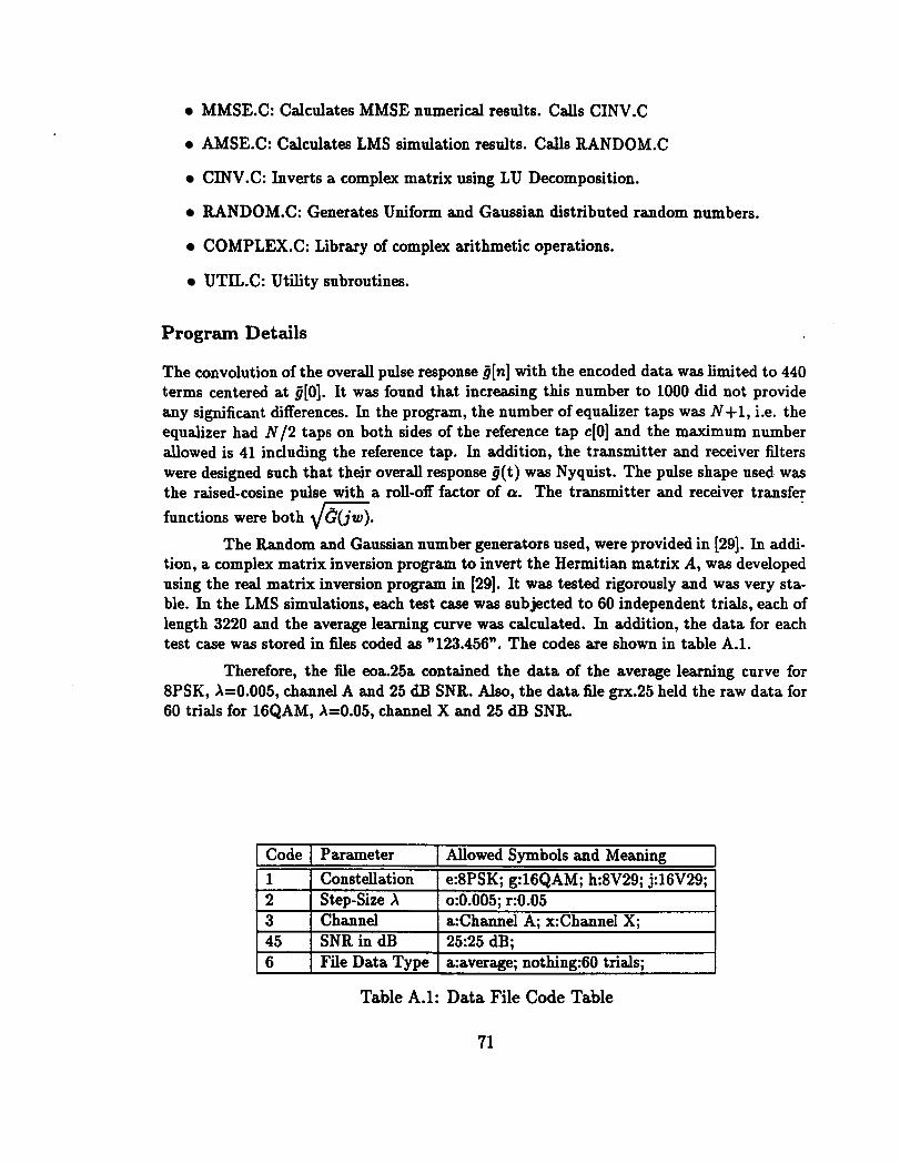
MMSE.C: Calculates MMSE numerical results. C d s C1NV.C
AMSE.C: Calculates LMS simulation results. Calls RAND0M.C
C1NV.C: Inverts a complex matrix using LU Decomposition.
RAND0M.C: Generates Uniform and Gaussian distributed random numbers.
C0MPLEX.C: Library of complex arithmetic operations.
UT1L.C: Utility subroutines.
Program Details
The convolution of the overall pulse response g[n] with the encoded data was limited to 440 terms centered at J[0]. It was found that increasing this number to 1000 did not provide any significant differences. In the program, the number of equalizer taps was N+1, i.e. the equalizer had N/2 taps on both sides of the reference tap c[O] and the maximum number allowed is 41 including the reference tap. In addition, the transmitter and receiver filters were designed such that their overall response #(t) was Nyquist. The pulse shape used was the raised-cosine pulse with a roll-off factor of cr. The transmitter and receiver transfer
functions were both 4 G . The Random and Gaussian number generators used, were provided in [29]. In addi-
tion, a complex matrix inversion program to invert the Hermitian matrix A, was developed using the real matrix inversion program in [29]. It was tested rigorously and was very sta- ble. In the LMS simulations, each test case was subjected to 60 independent trials, each of length 3220 and the average learning curve was calculated. In addition, the data for each test case was stored in files coded as "123.456". The codes are shown in table A.1.
Therefore, the file eoa.25a contained the data of the average learning curve for 8PSK, A=0.005, channel A and 25 dB SNR. Also, the data file grx.25 held the raw data for 60 trials for 16QAM, k0.05, channel X and 25 dB SNR.
Table A.l: Data File Code Table
Code
1 2 3 45 6
Parameter
Constellation Step-Size X Channel SNRin dB File Data Type
Allowed Symbols and Meaning
e:8PSK; g:16QAM; h:8V29; j:16V29; o:0.005; r:0.05 a:Channel A; x:Channel X; 25:25 dB; a:average; nothing:60 trials;
MMSE Program File and Test Case
#define HAX 256 /* H u number of signals in constellation */ #define OFFSET 220 /* Position of Reference Response */ Mafine HAXTEWS 440 /* Pumber of term8 in Convolution */ #define HAXTAPS 40 /* Haximum Number of Taps in Equalizer */ #def ine 1m 2 /* Used for Print Display */ #def ine PI 3.141592664 Mefine EUUOR 0.00000001
typedef rtruct FCOHPLEX i double r,i; 3 f complex;
......................................................................... /********* H - number of signals in constellation ++++*****+*/ /*******a* 1+1 - Total number of Equalizer Taps ********c**/ /********* SIG-SET - Signal points in Constellation *******+*+*/ /********* g - overall impulre r e s p o ~ e ***+L******/ /********a f - receiver impulse response ********+**/ /********* fp - file pointer to output data file *++**++***+/ /********* val - stores step-sizes that will be u m d in simulation *****/ /********* 10 - noise power to signal energy power *****+*++**/ ......................................................................... double HIPHEAPSQ~(H ,I ,SIG,SET .g .f ,f p ,val,NO) int H, 1; icompiex SIG,SETCHAX+II , ~ U U X ~ ~ + I I , I [IIIXTEWS+II ; FILE *fp; float val CPm+il, 10 ; i
......................................................................... /****************** Complex Operators ******&*********++***************/ .........................................................................
double Cabs ( ) ; fcomplex Caddo, CsubO, CmulO, Cdiv(); fcomplex ComplexO, ConjgO, ArgO, RCmulO;
......................................................................... /********** y - received signal, b - input data signal ***************/ /********** bd - differentially encoded phase *+*************/ /******a*** A - y correlation matrix, IPV - A inverse ***************/ /********** B - cross - correlation matrix bet. b and y ***************/ /********** C - equalizer vector *I************+/ /*****a**** USE - mean sqrure error, pdt = 1 - USE ***************/ /a********* dummy - dummy variable *****+*+**+**+*/ /********** v - rum of zln-il*e C j (sum of angler)] ***+*********+*/
......................................................................... f complex A [HAXTAPS+l] mXIAPS+l] , IIV ~XTAPS+I] [HAXTAPS+~] ; icorpiex I UUXTAPS+II CHAXTAPS+~I ; f complex B WXTAPS+l] , C mX TAPS+ll; f complex pdt ; double HSB;
......................................................................... /********** Cd, Cs vectors calculated during ideal gradient algorithm **/ /********** AC - pdt estimate of A matrix and C matrix *****************/ /********** I - Identity matrix, A1 = I - A t**++***********+/
......................................................................... f complex cd[HAX TAPS+l] , Cs [HAXTAPS+ll; f complex AC CHAXTAPS+ll; f complex A1 [HAXTAPS+l] ~XTAPS+l] ;
......................................................................... /********** i, j ,k ,kl ,kk ,n - indices, rn - random # generated *******/ /***a****** POI - reference point, jPm = j%Pm ******a/
/********** iff - mean square difference without equalizer **+****/ /***a****** Store, Store2 - intermediate differences **a****/
/********** alpha - step-size *******/ /********** cinv - hverts complex matrix *******/ /********** ran1 - generates uniformly distributed r.v *******/ /********** gasdev - gonerates gaussian distributed r.v *******/ /********** noise - additive chamel noise components at diff. instants*/ /********** w - noise after passing through receiver *******/ .........................................................................
int i, j, jPm, k, n; int mar-num, chk; float alpha ; double Dif f , Store, Store?; void cinv() ;
.........................................................................
......................................................................... for (i=O ; i<=HAXTAPS ;I++) < BCiI = Complex(O.0,O.O); for (j=O;j<=HAXTAPS;j++) ACil Cjl = Complex(O.0,O.O);
3 for (i=O ; i<=HAXTAPS ; i++) C [I] = Complex(0 .On 0.0) ;
for (i=O;i<WXTAPS;i++) gCi1 = Complex(O.0,O.O); for (i=O;i<WXTAPS;i++) gCWX1EBIIS-i] = Complex(O.0,O.O);
, . . . . . . . . . . . . . . . . . . . . . . .
for (i=l;i<=I+l;i++) B ti1 = Conjg(g Ci+OFFSET-I/2-11) ;
/***** Invert. A to IIV, dim I+l, A rmchanged ******/ cinv(A*1IVsI+l) ; f f lurh(fp) ;
, . . . . . . . . . . . . . . . . . . . . . . . . . . . . . . . . . . . . . . . . . . . . . . . . . . . . . . . . . . . . . . . . . . . . . . . - I
/**************++*+******** Opt- Qaalizer ............................ ..........................................................................
pdt = Complex(O.0,O.O); for (it1 ; i<=I+l ; i++) C cci-11 = Complex(O.O,O.O) ; for (j=l;j<=I+l;j++) CCi-13 = Cadd(CCi-11 ,Cnml(IIVCil Cjl sBCjI 1) ;
pdt = Cadd(pdt,Qnrl(Conjg(BCi'J),CCi-11)); 3 f f larh(fp) ;
..........................................................................
.............................. check to nee AC = B .......................
.......................................................................... /*
for (i=l ;i<=H+l ;i++) C ACCil = Complex(O.0,O.O); for (j=l; j<=I+l; j++) ICil Cjl = Complex(0.0,O.O) ;
ICil Cil .r = 1.0; 1 for (i-1 ;i<=l+l ;i++) i for (j=l; j<=li+l; j++) ACCil = cadd(~cCi1 ,Cmul(ACil [jl ,CCj-11)) ; if (ieh == 1) fprintf(fp,"W); fprintf (fp,"~t%3dl=Y.8.4f,%8.4fj *@,i,~cCil .r,Aclil .i);
3 f f lruh(fp) ;
*/ .......................................................................... /**************** Theoretical Interart - Ideal Grad. Alg. ***************/ /***************** c [i] = c [i] (1 -alpha x A) - alpha x B *****************/ .......................................................................... /*
fprintf (fp,"bb ***** HEAH SQUAFLE GRADIEIll UGORITEH ****#*I ;
for (chk=l ; chk<=max-nun; chk++) < for (i=O;i<=MXTAPS;i++) CCi] = ~omplex(O.0,O.O); if (DO) ~[l/2+l].r = 1.0; elre CCO1.r = 1.0; alpha = valCchkl ; f printf (f p , @@balpha=Y'. 4f \n" ,alpha) ; if .(alpha != 0.0) < for (it1 ;i<=l+l ;i++) for (j=l;j<=l+l;j++) AlCil Cjl = Csub(ICi1 Cjl ,RCmul(alpha,ACil Cjl)) ;
k=O ; do i k++ ; for (i=l;i<=l+l;i++) i ACCil = Complex(O.0,O.O); Cr Cil = C Cil ; for (j=l; j<=U+l; j++) ACCil = Cadd(ACCi1 ,Cmul(AlIil tjl ,CCj-11));
1 for (i=l;i<=U+l;i++) C [i-11 = Cadd(AC Ci] ,~Cmul(alpha ,B [i] ) ) ;
Diff = 0.0; for (i=O;i<=l;i++) CdCiI = Crub(CCi1 ,Cr Cil 1 ; for (i=O;i<=P;i++) Dif f += Cabs (CdCil ) ;
1 while (Diff > ERROR);
v = Complex(O.O,O.O); for (i=l ; i<=l+l; i++)
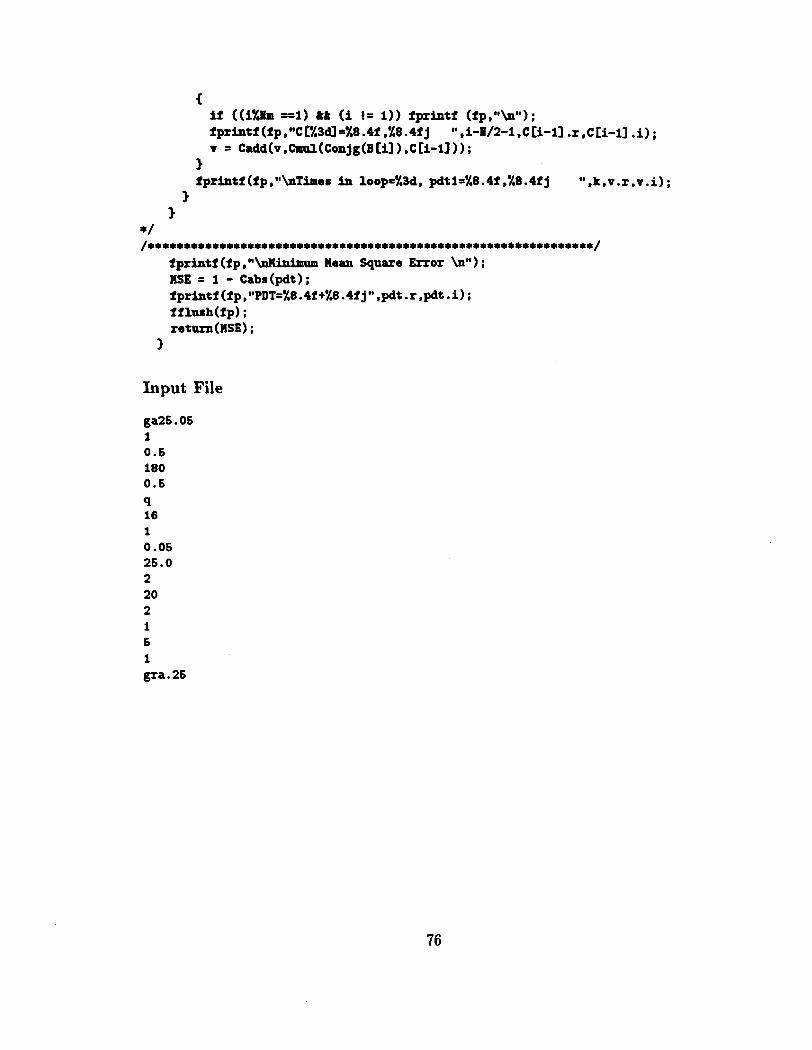
C if ((iYJm ==I) && (i != 1)) fprintf (fpSn\n"); iprintf (fpSwCrL3d=%8 .4f ,%8.4f j " A-112-1 rC[i-ll .r,C[i-11 .i) ; v = Cadd(v,rrul(Conjg(B[i]),C[i-11));
3 fprintf(fprwbT~erinloop=%3d,pdtl=%8.4f.%8.41j ",k,v.r.v.i);
3 3
*/ .................................................................
f printf (f p , ~o\nninimum Hean Square Error b" ; HSE = 1 - Cabs(pdt1 ; fprintf (fpSwPDT=%8.4f+%8.4f j" ,pdt .r,pdt .i) ; fflush(fp) ; return(HSE) ;
3
Input File
ga26.06 1 0.6 180 0.6
'I 16 1 0.05 25.0 2 20 2 1 6 1 gra .26
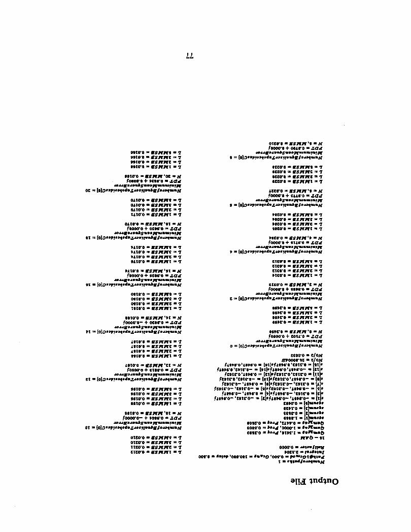
981QO P S R R 9 = 7 9910'0 = P S R R C a 7 981QO P S R R C 3 7 n t r o = PSRRI 3 7
981CO = P S R R '02 = N FOQOQO + ~ C O = raa
r o u ~ a r v m b ~ n v a p m u + ~ ~ OL = [ 0 ] 3 * W ? * q * d * r a = ? m P ; o - m ~
OLIQO = P S R R 9 = 1 OLIQO P S R R C = 7 OLIQO = U S R R C f 7 ILIQO = P S R R I ' 7
U 1 0 0 = P S R R 9 7 UIQO = P S R R C ' 7 UIQO P S R R C 7 9AIOO P S R R I = 7
UIQO ' P S R R ' 9 I I N .~WOQO + sctco = & a d
r o n p m r s m b ~ ~ - a e s u ? n ? ~ 91 = [ O ] ~ * V ? * Y * ~ * & U = ? ~ P # O - Y ~ N
- - -
ISIQO = P S R R I = 7
OIIUO f U S R R ' P I = N foooro- + ocrro = raa
r o u ~ a r v m b ~ n v a p m u ? r ~ P I 3 [ O ] ~ * ~ * ? . ~ ~ * ~ S . G ~ = ! F ~ ~ P I O ~ Y U ~ N
L8IPO = PSRRC ' 7 88IQO P S R R 1 7
96IQO = P S R R 9 0 7 96IQO P S R R C ' 7 PIIQO = P S R R L 17 861QO * P S R R I 3 7
OILCO = P S R R 9 7 OILQO ' P S R R C = 7 IICQO BSRRC 7 CILUO P S R R I 7
OICWO = P S R R 1 8 = N fooowo + 06~6-o = & a d
r o u @ a r v 3 ~ n v w p m u + ? ~ 8 = [ O ] ~ * ~ ! * Y * ~ * & Y . ? P * E ~ O ~ Y U ( . N
WLQO = P S R R 9 1 8ZLUO 0 P S R R C = 1 tCLQO P S R R C f 7 6CCQO P S R R I ' 7
LLCCO = U S R R . 9 = N f o o w o + crrco = raa
r o u p a r d s n m a p m m ? n ? ~ 9 [ 0 ] 3 * i * ? * q * d - & ~ * ! F d P ~ ~ u 1 y m N
W8LCO = PSRR'P N .COOOQ'O + S I L C O = raa
r o n ~ a r d y n v a ~ u m u ? n 8 ~ P " [ 0 1 3 * ~ ! * ~ * ~ - + a = ? ~ P ~ o r Y ~ m N
CICQO = P S R R 9 0 'I CICQO = PSRRC = 7 CICQO P S R R L 7 PIC00 = P S R R I 7
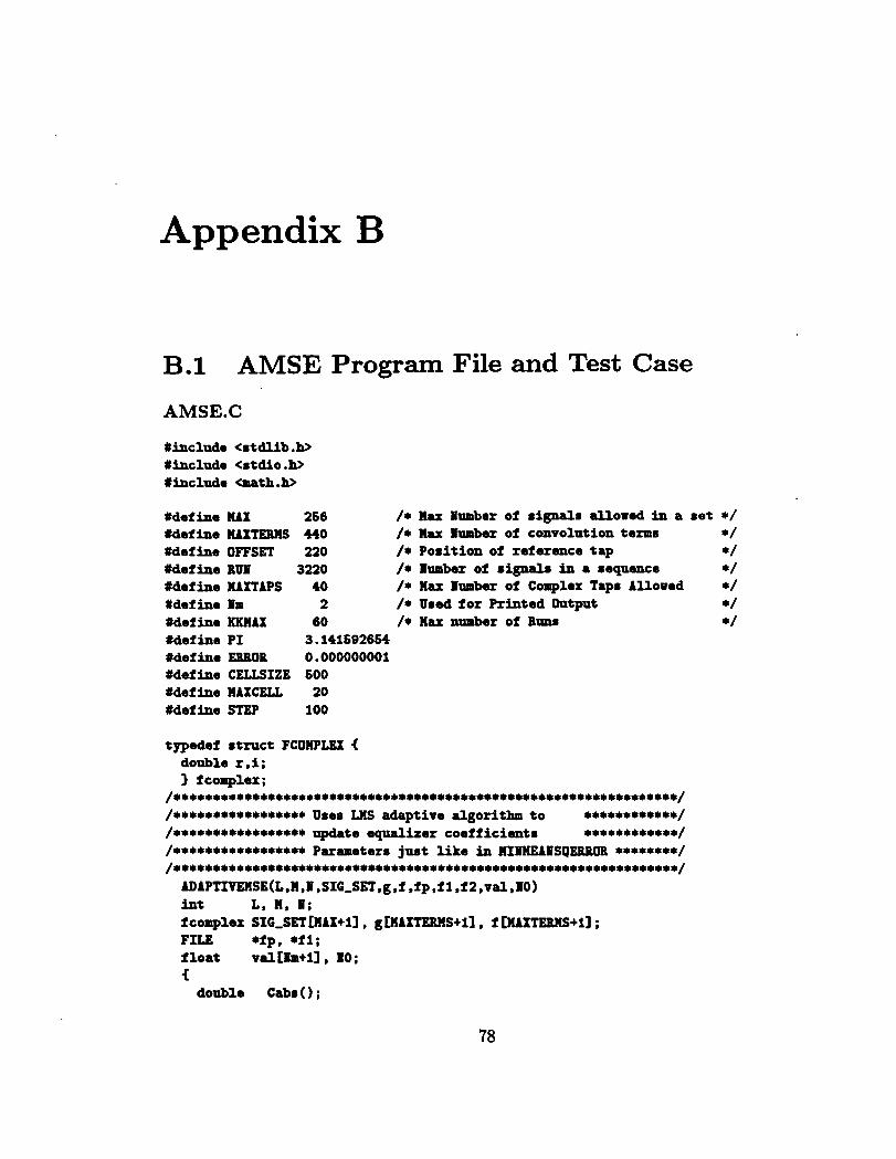
Appendix B
AMSE Program File and Test Case
Xdef ine l u x 266 /* Max Pumber of signals allowed in a se t */ Wefine HAXTEUS 440 /* M a x lumber of convolutiontermr */ #define OFFSET 220 /* Position of reference tap */ tdef ine RUE 3220 /* lumber of signals in a requcmce */ #def ine HAXTAPS 40 /* Hax Iumber of Complex Taps Allowed */ #def ine Im 2 /* Used fo r Printed Output */ #define KKHAX 60 /* Hax number of BUM */ #define PI 3.141692664 #define EBBOR 0.000000001 #define CELLSIZE 600 #define HAXCELL 20 #define STEP 100
typedef s t rac t FCOIIPLEX ( double r , i ; 1 f complex ;
/88~8888888888~~8888888888888888888888888~88888~888888888888888888/
/8+88*8*+++8+8888+ Uses adaptive algorithm t o 88888~**8***/
/***************** update equalizer coefficiants +**+******++/ /***************** Parameters juat l i k e in HIIHEAPS~EWOR ********/ ...................................................................
ADAPTIVEHSE(L,H,li ,SIG,SET,g,f ,fp,f l,f2,val,IO) int L, H * r ; f complex SIG,SET[HAXtl] , gCHAXTERXS+ll, f CnrXTERHS+l] ; FILE *fp, *f 1; f loa t val l l m t i l , 10; i
double Cabs() ;
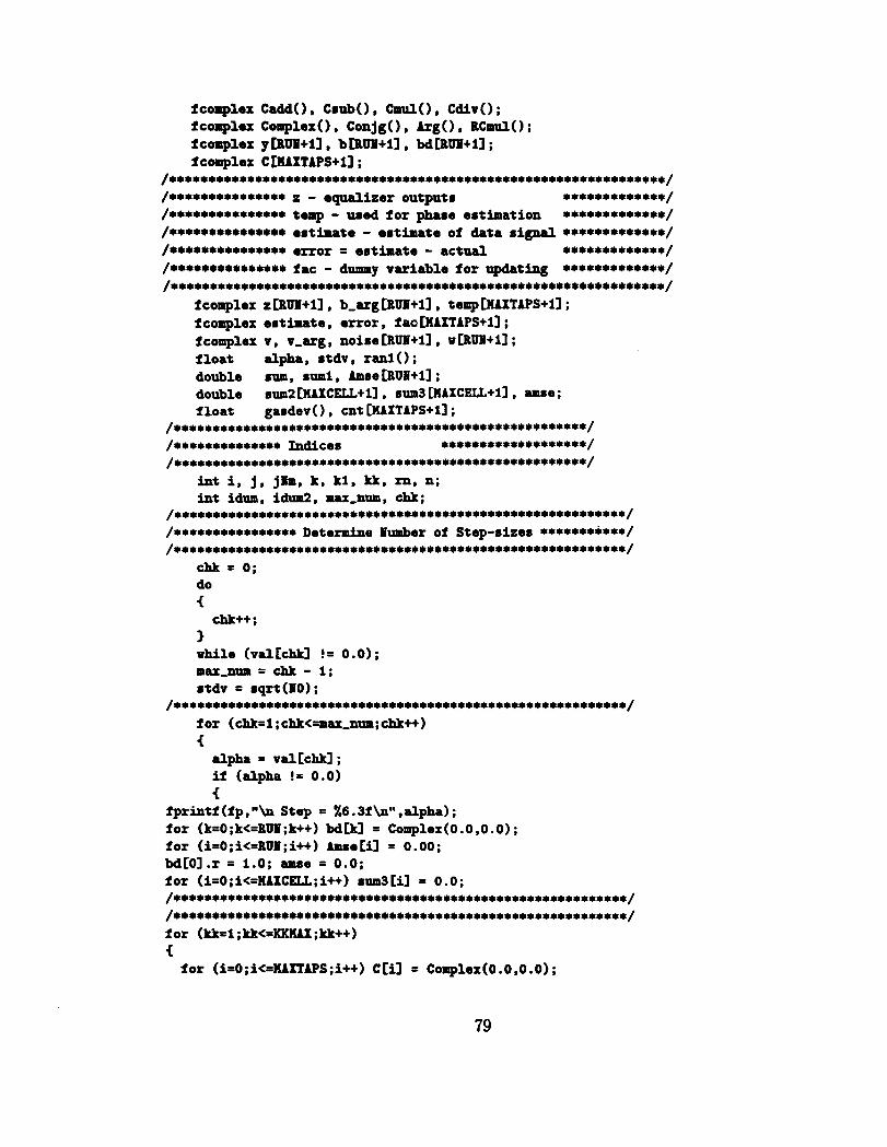
fcomplex CaddO, CrnbO, C m u l o , C d i v o ; fcomplex Complex0 , conjgo , Argo 8 R W O ; fcomplex ylsmr+ll, bCaUB+ll, WCaUB+lI; f complex C CHAXTAPS+ll;
.................................................................. /*************** - eqaalizer oatputr $****+C******/
/*************** t e l p - f o r ph.86 .stirpation *************/ /*************** a r t i r a t e - ertirpate of data rim *************/ /*************** er ror = estirpate - acts ******+**+***/ /*********+***+* fat - d m y variable f o r W t i n g *************/ ..................................................................
icompiex z CRUB+~I , b,arg CRUB+~I , temp cnrxTrPs+i] ; f complex estimate, error , f ao [lIAXTAPS+ll; f complex v , v-arg , noise CRlJU+ll , w CRUU+ll; f l oa t alpha, r t d v , r a n l o ; double rum, rum1 , Amse [RUP+ll; double rum2 [nAXCELL+l] . sum3 [HAXCELL+~] , amse ; f l oa t gasdev ( ) , cnt [UXTAPS+I] ;
........................................................ /************** Indices ************c******/ ........................................................
int i, j, jPm, k, kl . kk, rn, n; i n t idum, idum2. max-num, chk;
............................................................. /****+**********I Det0-e Bumbar of Step-sizes ***********/ .............................................................
chk = 0; do <
chk++ ; 1 while (valCchkl != 0.0) ; max-num = chk - 1 ; rtdv = sqrt(ll0);
............................................................. f o r (chk=l;chkC=max,num;chk++) <
alpha = vallchkl ; i f (alpha != 0.0) <
fpr intf(fp,% Step = %6.3f\nW,alpha); f o r (k=O;kc=RlJU;k++) M a 1 = Complex(O.0,O.O); f o r (i=O ; ic=RDll; i++ ) Amse Cil = 0.00 ; WCO1.r = 1.0; amse = 0.0; f o r (i=0 ; ic=nAXCELL ; I++) sum3 Cil = 0.0 ; ............................................................. ............................................................. f o r (kk=l ;kkc=KKHAX ;kk++) <
f o r (i=O ; ic=JIAXTAPS ;i++) C Cil = Complex (0.0 ,O .O) ;
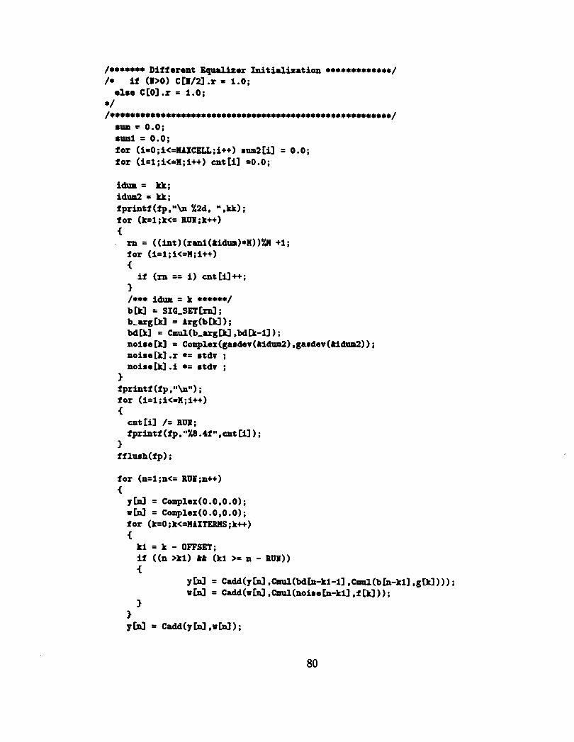
/******* Different Equalizer In i t ia l iza t ion *************/ /* i f (DO) CC1/2l.r = 1.0;
e l se CCOI .r = 1.0; */ ..........................................................
8m 0.0; sum1 = 0.0; f o r (i=O; i<=HAXCELL;i++) sum2 Cil = 0.0; f o r (i=l;i<=H;i++) cn t t i l tO.0;
id= = kk; id& = kk; fpr intf(fprW\n %Id, "Skk); f o r (k=l;k<= BOP;k++) i . rn = ((int)(rml(&idm)*H))YJ +l;
fo r (i=l;i<=H;i++) i
i f (rn == i ) cntCil++; 1 /*** id= = k ******/ b W = SIC-SETCd; b,argW = Arg(bCk1) ; b d w = Cmrrl(b,argW ,WCk-11); noise [kl = ~omplex(gasdev(ltidnm2) .gasdev(Lidud ) ; noireCk1 .r *= stdv ; noiseW .i *= stdv ;
1 fprintf (fpSw\n") ; fo r ( i = l ;i<=H;i++) i
cat Ci3 /= BOP ; fprintf (fp . "X8 .4fW, cnt Cil ;
3 ffllmh(fp) ;
fo r (n=l;n<= BmJ;n++) i
yM = C0mp1ex(0.0.0.0); OM = Complex(o.O,O.o); fo r (k=O ; k<=HAXTERHS ; k++) i
k l = k - OFFSET; i f ( (n >kl) && (hi >= n - BOP)) C
y M = Cadd(y M ,Cnml(bdCn-kl-11 ,Cmul(bCn-kll ,gCkl))) ; w h d = Cadd(wM ,Clmil(noiseb-kll ,f Ck]));
3 1 y h d = Cadd(yM .wM);
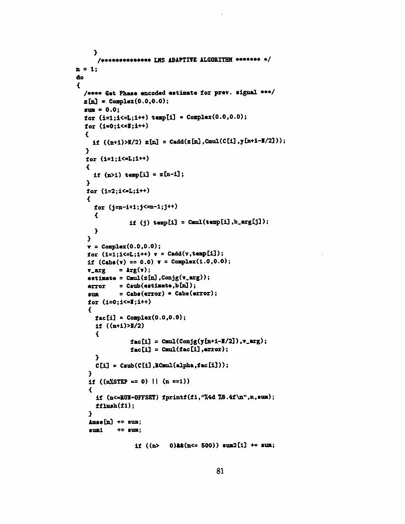
3 /*+************ U S ADAPTIVE UGOBITEH ******* */
n = 1; do i
/**** Get Phase encoded estimate for prev. signal ***/ zIn3 = Comple.(O.O,O.O); sum = 0.0; for (i=l;i<=L;i++) teopp[il = Complex(O.0,O.O); for (i=O ; i<=I ; i++) i
if ((n+i)>E/2) zlnl = cadd(z Cd ,Cmul(c Cil ,yb+i-I/21 ) ) ; 3 for (i=l;i<=L;i++) < if (n>i) templil
1 for (i=?;i<=L;i++) < for (j=n-i+l; j<--1; j++) i
1 v = Complex(O.O,O.O); for (i=i ;i<=L;i++) v = ~add(v ,tempCij ) ; if (Cabs(v) == 0.0) v = ~omplex(1.0,O.O); v-arg = Arg(v) ; estimate = ~mul(zCnj ,Conjg(~-arg)) ; error = ~aub(eatimate ,bid ; sum = ~abs(error) * Cabs(error); for (i=O;i<=P;i++) i facCi1 = Complex(O.O,O.O); if ( (n+i >I/2 1 <
factil = Cnml(~onjg(yCn+i-1/21) ,v,arg) ; facti] = Cmul(facCi1 ,error);
3 cCi1 = Csub(CCi1 ,BCniL(alpha,facCil));
3 if ((nfSTEP == 0) 1 1 (n ==I)) i if (n<=BUH-OFFSET) f printf (f 1, "%4d X8.4f \n" ,n, sum) ; ff lUsh(f1) ;
1 AlllseCd += sum; sum1 += sum;
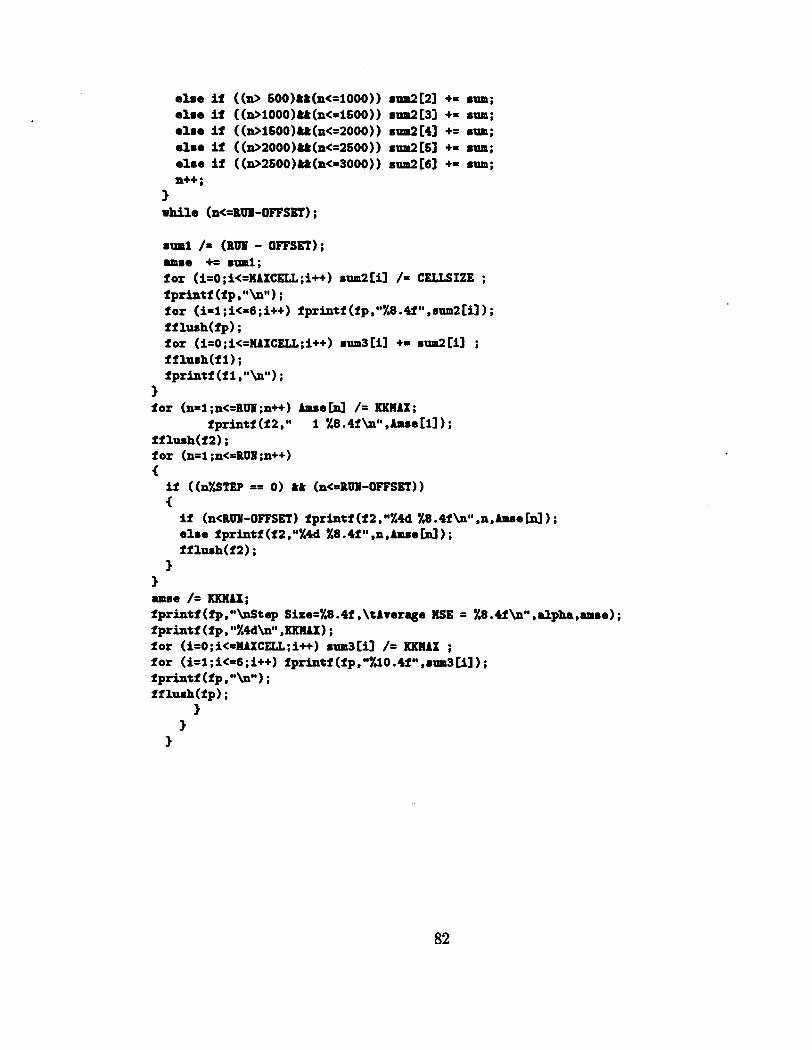
rum1 /= (Bull - OFFSET); m.0 ++ 8-1; for (i=O ; i<=HAXCELL ;i++) s1m2 [il /= CELLSIZE ; fprintf (fp,"\n") ; for (i=l ;i<=6 ;i++) f printf (f p ,"%8 .4fM ,sum2 [il) ; f f luah(f p) ; for (it0 ; i<=HAXCELL;i++) rum3 [i] += rum2 ti] ; f f lush(f I) ; fprintf (f I ,"\n") ;
1 for (n=l ;n<=Bm;n++) Amse bd /= KKHAX ;
fprintf(f2," I %8.4f\n",limse[l]); f f lurh(f 2) ; for (n=l;n<=RUU;n++) C if ((nYSTEP == 0) && (n<=BUli-OFFSET) ) C if (n<BUli-OFFSET) fprintf (f 2, "%4d %8.4f \nu ,n,Amae bd ; else fprintf (f2,"%4d %8.4f",n,Amrebd) ; fflush(f2) ;
3 3 amse /= KRIIAX; fprintf (fp ,"\nStap Size=%8.4f ,\tAver.ge W E = %8.4f \n" ,alpha,amse) ; fprintf (fp,%4d\n" lo ; for (i=O;i<=UXCELL;i++) rum3 Cil /= gglUX ; for (i=l;i<=6;i++) fprintf(fp,"%10.4f",rtrap3[i]); fprintf (fp,"\n") ; ffluah(fp) ;
1 3
1
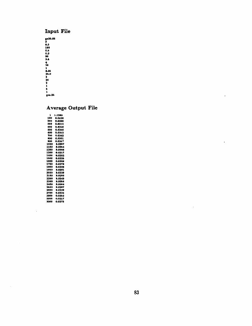
Input File
Average Output File 1 1.1100
100 0.0438 100 0.0186 300 0.0311 400 0.0116 600 0.0146 600 0.0311 TOO 0.0141 800 0.0301 900 0.0147
1000 0.0197 1100 0.0164 1300 0.0186 1300 0.031T MOO 0.0181 1600 0.0116 1600 0.0109 1700 0.03TO 1800 0.0318 lm00 0.0391 1000 0.0339 a100 0.0190 1100 0.0349 1300 0.0166 1400 0.0184 1b00 0.0167 moo o.orr9 1700 0.0334 a800 0.0am a900 0.0317 3000 0.01T8
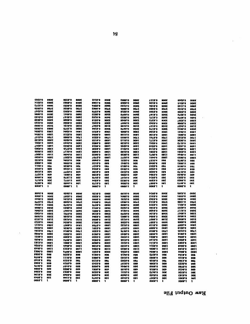
COCQO OOOC PICWO O M C CLCQO W I C 6 w o W L C L P L C O 001c vooo-0 W S C C V I C O ww 6 C W O OOCC OPCUO wcc 6600-0 W I C L O W 0 O W L *60QO ow1 VSOQO 0 0 8 1 L F I Q O 0 0 4 1 OCIWO OOVI I P C C O 0 0 9 1 L S D 0 0 OO*1 CVCCO OOCI I I O O - 0 OOCI L W O O wt1 OCCQO 0 0 0 1 C C I C O 0 0 1 0 0 0 C 0 0 0 1 I I W O 0 0 4 6tOQO 0 0 1 S O 1 0 0 0 0 9 L L L C O 00) 600QO OOC I L I W O OOC U S Q O 0 0 1 O O O r 1 I
OVPCO OOOC 8800'0 OO6C W P 0 ' 0 W I C U C O ' O OOLC P S I Q O OOOC I I W O wsc POSWO o o w COCWO OOCC I 1 O W 0 wcc 6 1 O I - 0 0 0 1 1 C I C C O OOOC I I t U O 0 0 6 1 CCCQO 0011 P S I 0 0 0 0 4 1 I I O C O 0011 I C W O W P I P S W O 0 6 9 1 C I I S O OOC1 PLCQO OOCI 6PPO-0 0011 C W O 0001 O ~ O U O 001 I L O C O m OPIQO 0 0 1 OVCQO 00, PLOCO 001 I 6 0 0 0 00) VOCPO 001 9610-0 OOC 6 w o - 0 001 O W Q I 1
s e w 0 oooc C I W O o m C C W O m c O C W O W A C CSCQO 001c 1 P I O O 001c LWIQO O O W VCCCO OOCL O m o ' O wcc I C I Q O W I C 1LOI.O OOOC PVCCO 0011 O I C C O W V I omo'o W L 1 OCCPO 00.1 C V W O 0011 C C W O wv1 SILQO W C I L I I Q O OOCI H W O 0011 L O C O 0 0001 H C Q O 001 O I W O 0 0 8 O C W O W L D W Q O 0 0 0 LLCQO 0 0 9 1 6 W O 0 0 ) O L o r o ooc ILCQO OOC II,O-0 0 0 1 OOQQt I
8090-0 OOOC L I C Q O OO6C P610-0 OOIC 6 V W O W A C 6LCQO OOOC CISQO wsc LSCCO W W IOAQO W C C P V I C O W C L t610-0 OOIC P C W O OOOC A w o 0 0 6 1 scsuo O W 1 P I W O 0 0 4 1 COCQO W O I 6OCWO 0 0 9 1 V L W O ww IOOQO m1 S U C O W C I C I C C O 0 0 1 1 l L W 0 OOOI 8sCQO 001 I I I C O 001 SICQO 0 0 4 SIZQO 001 LOIQO 001 C C W O 00, C W O 0 0 s 6 W Q O W C s w r o 001 O O O I I I
I P I Q O oooc n o r 0 oooc P O W 0 m e cmo'o W L C I L C C O 001c C C W O OOOL C I I Q O W W VICQO OOCC S I W O W C C LPCCO W I C PVIQO 0 0 0 C O I C C O w11 nwo oorr I I C Q O W L I CCIQO w,1 c o w 0 0011 I I W O W P 1 occwo OOCI W W O W C I C C W O 0 0 1 1 LOLOO OOOI 0 1 W O OM CCIQO 001 L C I U O 001 t P S Q 0 0 0 1 0 1 I C O 0 0 s I 1 1 C O 00, VLSCO W C WCQO OOC I A I Q O 0 0 1 oooc-0 I
PCIQO O W C SSCQO 006C S600-0 OOIC wow0 W L C 6 L L C O wvc L I W O 001C IOOQO ww W I Q O m c n c u o w u I I W 0 OOIL C I W O OOOC I I L Q O OM1 1 W Q O 0 0 1 1 SCCQO W L I 6 I W O 0 0 0 1 CCCQO 0 0 9 1 W W O W P I 6 C W O OOC1 W I C O wct H C C O W I I 1owo 0001 S I I Q O 001 CIOQO 001 C C I Q O 0 0 1 CPCQO 001 8 s W O 0 0 s IOOQO 00) VCCQO 001 O 6 W O OOC I L W O 0 0 1 OOOQI I
CIOQO OOOC 1 ~ C O OOIC W I Q O Wit S I O Q O W L C OICQO 0 0 1 C 6 L W O m c C C W O W P L O W 0 OOCC L O W 0 W C C W I Q O OOIC OLSCO OOOC P I W O 0011 I O I Q O W I I C C W O 0 0 4 1 C I I C O 0 0 1 1 O C I C O 0011 O W C O 00,I LICQO OOCI 6010-0 ooc1 I C W O 0011 LLCQO 0 0 0 1 I C C C O OQ. I W O 001 c m r o WL C W W O 00, L I I Q O 001 V6LQO 00) L V I Q O OOC CLOCO OOt VSOQO 001 0000'1 1
6 1 I C O OOOC ,wo-o owe I O I Q O W I C C C W O W L C O I I C O 0 0 1 C C C W O 001c I K C C O W P C OLCUO W C C CObQO wcc C C I U O W I C WCQO OOOL C C I C O OQ.1 LOCCO 0011 OLSCO 0011 O P W O 0 0 8 1 COCQO 0011 W 1 U O wv1 181QO OOCI L 6 I C O W C I C C W O 0 0 1 1 rnro 0001 I I W O 001 C O I U O 001 CVCQO 0 0 1 L O W 0 001 vvw-0 001 S I I C O 00, I S I Q O OOC 1 O W O wc 6 C I Q O W I w o r t I
L I I C O oooc PCIQO 001C S V I C O OOIC L I W O W L C O I C C O W V C AVIQO 001C I L I Q O W W CLCQO W C C CPCQO wcc L C I C O W I C PLIQO OOOC I I I C O O O I I O C I C O 0 0 8 1 I l L C O W L I I L I Q O o w 1 I P C C O 0011 0 1 w o W W * I I Q O m1 I W C O wet I L P Q O 0011 I S W O 0 0 0 1 L S I C O 001 O V W O wv CWZQO W L OCCQO 00, O C W O 0 0 9 *VCQO 00, P I 0 0 0 om 6OCCO OOC LVVQO 0 0 1 mrt I
P I W O OOOC CICQO O W C CPCQ'O W I C P I I C O W A C C I C C O 001c S V I 0 ' 0 001c I C W O ww OCIQO m c P I I C O wcc L w 0 W I C L6CQO OOOC 6110-0 0011 6SCCO 0 0 8 1 6 I W O 0 0 4 1 O I O C O m1 M W O 0011 1 P I U O ww W I I C O OOCI * I C C O OQCt S C W O 0 0 1 1 W W O OQOI U C C O 001 CIOQO 001 SISQO W L S I C C O 001 6 S W O 001 S I W O 00, U W O OOC COIQO we LVCQO 001 O O O r 1 I
1PCQO OOOC OICQO 001C 0 v 1 r 0 001c W I Q O W L C 6CCQO W V C U O O - 0 wsc 1 A W O W V C A ~ C C O wcz e w o WCL L S W O W l C P180'0 O W C I I S C O 0 0 6 1 I I W O W I I C V I C O W L I PCOCO wor U I Q O O O I I CCOt'O W P I OIOQO OOCK W C C O OOCI W W O 0 0 1 1 C C W O OOOI P L W O ow C O W 0 0 0 1 O I O C O OOL 1810-0 00, 6 L I Q O 0 0 9 OCPCO 00, C6CO-0 OOC 6 W O OOC CLOQO 0 0 1 OOOCO 1
saro-o woc ? I C C O owc C O W 0 W I C 01Cl'O OOLC 1 1 W O W V C CCCCO OOSC A I I C O OOW L P W O m c ocW0 W C C P I W O W I C I m o ' O OOOC L O W 0 0 0 6 1 O I W O 0 0 8 1 SOIQO OOLI V I W O oOv1 V I D 0 0 0 0 9 1 C I 1 C O w*1 C6CQO W C I O W 0 W C I I V I C O 0011 o w 0 OOOI W I Q O 001 S I I C O 001 1SCI-0 OOL U C Q O 001 W L W O 001 O I W O OQ, OCCUO OOC CVIQO W C COCWO 001 OOQCt I
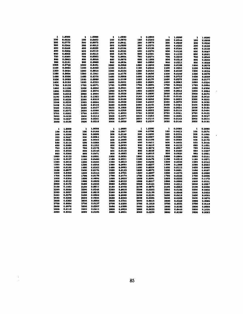
I 1.0000 100 0.0796 100 0.0011 300 0.0067 400 0.0198 660 0.0411 MO 0.0410 TOO 0.0074 MO 0.0039 m 0.0010
1000 0.0131 1100 0.0416 law 0.01u 1 ~ 0 0 o a m 1400 0.0019 1600 0.0073 1600 O.Oao? 1 m 0.0189 1800 o.oo.1 1WO 0.0011 1000 0.0163 1100 o a o n 1100 o.Oao3 1so0 0.0138 1400 0.0186 1600 0.0306 1800 0.0016 1700 0.1019 am0 0.0016 aeon 0.0011 so00 0.0119
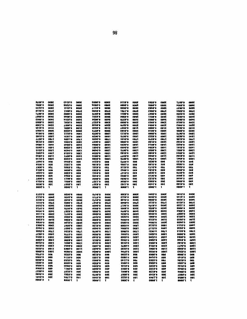
O L W O oooc I I O Q O 0 0 6 C C C I C O W 8 C 0 1 1 ~ 0 W A C I L 1 0 ' 0 m c LO8CO W P C C000'0 ww 0 9 W 0 00CC 68CI.O W C C 9PtO-0 W I C C P W 0 OOOL I 1 W O 001t 0 8 1 C O 0 0 8 1 LLOWO W L I O C I C O , 0 0 1 1 0900 '0 0 0 9 1 COPCO OOPI 91co-0 00tI IOCO-0 W C I CCOCO 0 0 1 1 0 1 1 ~ 0 OOOI L W C O 0 0 6 I C O C O 0 0 8 LSOCO 0 0 4 P I O C O ow OCCCO 0 0 9 6 6 0 0 ' 0 W P L a w 0 o o c C I C C O W C P C W O W I oooc-0 I
CLCCO OOOC C I I C O Wac CC9CO 0 0 8 C I C I O ' O 00LC 0910-0 OOOC 9 I L C O W 9 C W O C O ww 9P11'0 W C C 8CCCO W C C 6 8 C C O wtc 8 0 0 Q O OOOC COOCO 0011 C W C O 0 0 8 1 9OC0O OOLI LCSCO 0 0 8 1 s 9 w o OOPI 68CQO W P 1 8 0 1 0 0 O O I I POIWO W C I OCCUO 0011 9 m o OOOI 90LQO 001 8 9 C Q O 0 0 8 O C W O 0 0 L CCtO-0 ow s 9 w o 0 0 9 8 9 0 0 ' 0 00, LCOWO 0 0 s O 6 W O W C I O I C O 0 0 1 0 0 0 C 0 I
C P I C O OOOC wcco ooec 1P10-0 W I L I I W O W L C C610'0 W S C O I W O OOIC P I C C O ww 1 6 W O OOCC L 9 W 0 OOCC t a w 0 W I C CCCCO OOOC 11100 O O I I w r o W ~ I S6CI-0 W L I C 0 C C 0 wo1 O * W O 0 0 9 1 68CO-0 W P 1 8 C W O OOCI O I C C O OOCI I L O C O 0 0 1 1 aomo o o o r O W C O 0 0 6 CCOI-0 0 0 8 9OCCO 0 0 4 srwo wo 8OCWO 0 0 9 W C C O 00, c110'0 0 0 c ICOQO OOC L O W 0 0 0 1 oooo-1 1
OCOCO oooc 9CCCO 006C 0810 '0 OOIC ~~~~0 OObC c a w 0 OOOC 9 L W 0 OOPC L I C C O O O W I L W O m c S9CQO OOCC OICQO 0 0 I C S O W 0 OOOC L6OQO 0 0 6 1 LOOQO 0 0 8 1 F 8 1 C O 0 0 L I SLLCO 0 0 9 1 C6OCO O W 1 0 6 C C O 0 0 P 1 I C W O 0 0 C I C 9 W O W E 1 c m o 0011 8 C W O OOOI 9CCCO 001 P11WO 00, C 9 1 0 0 0 0 1 W C C O 0 0 8 O W C O 0 0 9 1 1 W O 00, L810-0 W C I8CO-0 o o c POLI-0 0 0 1 O O W I 1
c w o W I C O A I I C O 0 6 W O O L W O ICCQO W W O ACCUO CC9CO 089QO CLCWO 6 L W O 6 C W O 9 , W O L C W O 9 9 W O I 6 W O wwo 6CCCO 9100-0 W C Q O 8ICO-0 9 6 I Q O I O I Q O C8CQO I W C O CCPCO O S W O LEC1'0 LPCCO OOOQ1
O L W O O I L V O CAPO-0 L V 9 C O 6010'0 6 C W O 9 I W O OPCQO LOIQO
' OOCQO 8CCCO O C I C O 6 9 W O OLOCO O C W O 0 P I C O 9190'0 8 I C Q O 8081 '0 c a w 0 *COQO OCIQO CC8I'O C W C O OCCCO POCCO 6 8 9 4 0 CCCQO 6 L W O 8 M I - 0 OOOO1
OOOI OQIC m c W L C m c OOIC OOVC OOIC OOCC W I C OOOC 001I 0 0 8 s W L I 00.1 O O I I W P 1 OOCI W C I 0 0 1 1 OOO1 0 0 6 0 0 8 W L W 8 0 0 9 00) W C OOC 001 t
oooc ooac OOIC OOLC wsc 0 0 9 C W P C OOCC wcc W I C owe 0 0 6 1 0 0 8 1 W L I 0 0 6 1 O W 1 00~1 0 0 C 1 we1 0011 O W 1 0 0 4 0 0 1 W L 0 0 s 0 0 9 00, OOC OOC wr 1
O I I Q O oooc osoo-0 m e 8 C W O W 8 C m r o WAC 1 1 8 C O m e S8CCO OOIC OLCQO W W 6 6 W O OOIC I b C C O W C C L W O W I C L 8 I C O OOOC C I I C O O O I I 8LOQO 0 0 8 1 9 9 I W O W b t moo-0 wst C C W O W I t 6 6 W O W P I 9bOQO OOCI C I W O We1 L A C 0 0 0011 8 L W O OOOI U C C O 0 0 4 9961'0 0 0 8 8 1 I C O 0 0 L C P W O 0 0 8 L V I C O W 9 C C W O 00) OCOCO 0 0 C 099QO W C CVI1 '0 0 0 1 OOOQI I
88CCO OOOC C I P C O W 6 C * P I C 0 OOIC O69WO W L C L I W O OOOC 0 8 W O OOPC OL6QO OOPC W C U O wcc C C W O W C C W C C O W I C C 9 8 0 0 OOOC 6 8 C C O O O I I P 8 W O 0 0 8 1 9wo-0 W L I 1 ~ 0 0 0 8 1 6 8 1 0 0 0091 C I I C O 0 0 C I 8 C I C O W C I W W O we1 OCCQO 0 0 1 1 W A C 0 OOOI 0 6 C ~ O 001 caw0 m 0 ~ 1 l ' O W L 9 9 W O 0 0 8 9,100 O W CCOCO 00, I 8 W O 0 0 s LSOQO OOC C C I C O 0 0 1 oOOC0 1
ClCO-0 OOOC 9080-0 OOIL C I W O W I C C 9 9 C O W L C A m 0 m c I I W O W 9 C C O W 0 W P C C860-0 wcc * S W 0 wcc 8 m O W I C 8 1 W O OOOC I W C O O O l I CCCQO O O t t OLCQO W L I esrro wsr V 1 W O 0091 W C O O W W 9 9 W O OOCI 8 I I C O W C I O I W O 0011 SILO-0 OOOI 9 C W O 0 0 6 8610-0 0 0 8 C L I C O OOL w 1 r o 00, 6 C W 0 0 0 9 O I O C O wv C C I C O W C COCCO wc 8 C v r O 001 OOOQI I
P8CCO OOOC e c o ~ o wrc erro-o wrc O I I C O W A C OLCCO woe 9 c w 0 W 9 C I C W O 00VC 8 W C O OOIC 1 m 0 W C C 9 I C C O 0 0 I C W W O OOOC 0 1 1 ~ 0 0011 L I I C O W 8 1 I C O C O 0 0 4 1 CSCQO 0 0 0 1 86CO-0 0 0 9 1 OOCQO 0 0 P I C 9 W O W C 1 OICQO wct 1 8 W O 0011 O C W O OOOI 600QO 001 m10-0 001 COCCO O I L C9CCO 00, C O I C O O W COIWO 00) 6 C 1 0 0 ooc 6PIO-0 OOlC e w r o OOI O O O Q I I
I L W O OOOC won-0 OQIC L C 9 C O W 8 C W C Q O W L C O I C C O woc I C W O OOPC C 6 9 C O ww O I W O OOCC C 9 W O wcc PCPCO W I C 9800-0 woe O L W O 0041 9 C W 0 0 0 8 1 9 6 I C O O O I I 8 9 1 C O 0 0 8 1 C C W O 0091 I 8 I C O 0 0 P 1 1 9 W O ooc1 P I W O OOCI n w o 0 0 x 1 t n w o OD01 C C I ~ O 00. 0 9 8 C O 0 0 8 8 W C O OOL 6800-0 0 0 9 I L W O 0 0 9 W W O 00, OC9CO OOC 1 6 W O W E 8810-0 W I O O O I I I
9610-0 oooc 8 P I C O 0 0 6 c PILO-0 O08C 6 I C W O W L C 8CC1'0 m e SsOQO w 9 c W W O W P C L W 0 OOCC O I W O wcc C C W O W I C 6 8 W O OOOC C I W O 0 0 6 1 OCCCO 0081 C I C C O W L I 0 ~ 0 00)I 0 9 W O O W 1 O C Q O 00M o t r r o oocr L L W O OOCI 68CO-0 0011 C9CCO OOOI OOOQO 001 P P I Q O 001 W I Q O 0 0 4 9 W P O 00, H I C O 0 0 9 W 9 0 0 00) t w o wc LOIQO wc W W O W I OQOCI 1
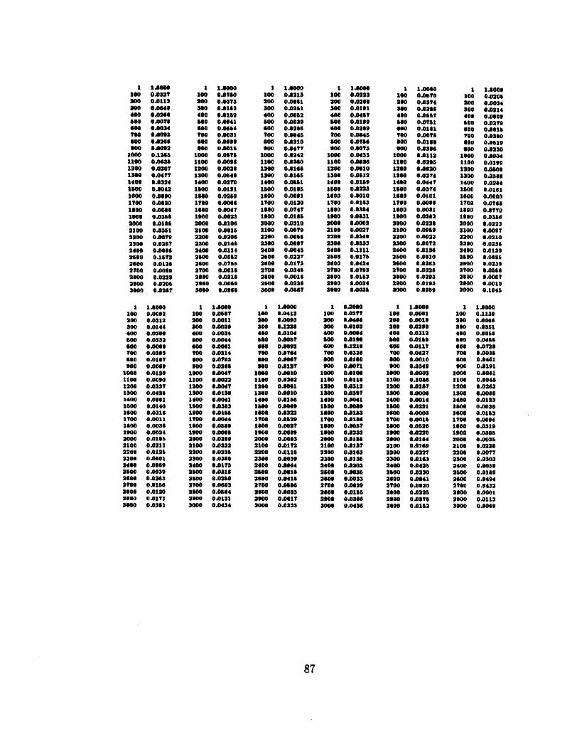
1 1 ~ 0 0 0 100 0.0317 100 0.0113 SO0 OW48 400 0.0166 MO 0.0078 MO 0.0034 700 0.0093 600 0.0188 MO 0.0091
1000 OJ166 1100 OWW 1100 0.0107 1WO 0.0477 1400 0.0314 1600 0.0043 1600 0.0090 1700 0.0010 1800 0.0098 1-0 0.0368 1000 0.0185 a100 0.0361 a300 0.0079 1300 0.0187 1400 0.0088 1500 0.15n 1600 0.0128 1700 0.0098 1800 0.0119 1900 0.0105 3000 0.0187
1 1.oooa 100 0.0113 m o m o r 500 0.0191 400 0.0457 MO 0.0190 MO 0.0189 TOO 0.0045 MO 0,756 MO 0.0073
1000 0.0433 1100 0.00s 1100 0.0010 1300 0.0511 1400 0.0159 1600 0.0313 1600 0.0010 1700 0.0183 1800 ObW4 1)Oo 0.0831 a000 0.0001 a100 0.0017 a100 0.0SIO 1m 0.0633 1400 0.1111 1500 0.0175 1600 0.0414 1700 0.0193 1800 0.0153 awo 0.0014 3000 0.0036
I O I W O OOOC t 9 9 C O 0 0 6 2 C ~ O U O OOIC 11c0.0 W L C O I I I O W I C 9LCO'O OO9C 9LIO-0 W P C 9 I O C O OOCZ 6 C I C O OOCC zc01'0 0 0 1 2 ~ 1 0 0 ' 0 O W L 9 6 9 U O 0 0 6 1 O I 9 C O W I I 6 I W O W b 1 occco oosr OC6CO 0 0 9 1 9b90'0 0 0 ? 1 9LCCO OOCI Z I 9 0 - 0 OOCI C801'0 0011 P I I C O 0 0 0 1 CCP0'0 0 0 6 96tO-0 0 0 1 C I C C O OOL 6 6 I C O 0 0 9 06CO-0 0 0 9 OICCO 00) 9900 '0 OOC 9 I O C O OOC CLCCO 0 0 1 OOOCO 1
C?00'0 OOOC 9POCO 006C 0910 '0 OOIC 1100 '0 OOLZ I L A 0 ' 0 OOOC 9110 '0 0 0 9 C SCS0'0 OOW 6 9 I C O OOCC L A I C 0 OOCZ CCOQO OOIC 1010'0 OOOC P C I C O 0 0 6 1 O6CO'O O O I I CCCO-0 OOLI I C C C O 0 0 9 1 o r w o 0091 U ? C O O O I t 69Ao-0 OOCI I 0 0 ~ 0 OOZI I v w o 0 0 1 1 9DCQO 0 0 0 1 C090'0 0 0 6 I 6 O C O 0 0 1 CCCCO 0 0 4 9110 '0 0 0 1 A 6 W O 0 0 9 9690 '0 0 0 ) ?CCCO OOC 9610 '0 OOC 9 9 9 C O 0 0 1 o o o r r I
6 1 W O OQOC LCCCO O M C O I C U O W I C SCZ0-O W L C *#COO W S C I C C C O w 9 t 6 C W O W P C L I W O W C C OCI1 '0 wet 9 C C I O 0 0 1 1 L W O OOOL W I Q O OM1 r o w 0 0011 C 9 W O W L I L C W O 0011 O L I C O 0 0 9 1 O I I Q O W ? 1 L W O OOCI M C O - 0 OOCI I I C U O W I I c *wo 0 0 0 1 9060 '0 O M I I ? 0 ' 0 0 0 1 9 L I C O 0 0 4 6CC0'0 We C 9 W O 0 0 9 C900'0 00, CLCWO o o c W 9 0 ' 0 OOC 91OCO Wt OOOCO I
I C O C O OOOC I C C C O 0 0 6 2 C000'0 OOIC CPC1'0 OOLC C I O C O OOIC 0010 '0 OOPC L I W O OO?C ALCUO OOCC IOLO-0 OOCC O H C O OOIC I C W O OOOC I L 6 0 - 0 0 0 6 1 LLCO'O O O I l WLV0'0 0 0 4 1 0 6 1 0 ' 0 0 0 0 1 L L C C O 0 0 9 1 6 C W O 0 0 P 1 O I I C O OOCI r c w o OOCI 9 c w o 0011 P 6 W O OOO1 C010'0 O M L C W O 0 0 1 ?600 '0 0 0 4 0 ~ 0 0 0 s C 6 W O 0 0 9 ICCQO 00, C O I Q O o a r CO9QO OOC I C C V O 001 O O W I 1
691QO OOOI I 9 I C O ooac H O C O OOIC IPtO-0 W L t e c w o m e M I Q O OOIC M I Q O W P C W W O OOCC CCIQO W C C CCCOO W I C 9 L W O OOOC C I I Q O 001I W W O W E 1 9 9 9 C O W L I I L C C O W I I ? 6 W O 0 0 9 1 L n r o 0091 W I I C O OOC1 L I W O W C I eaoo-0 0 0 1 1 1 0 W O OOOr I I C C O 001 L 9 W O 0 0 1 IOCWO 0 0 1 A 1 1 1 0 0 0 0 ? I W O o m L C W O 00, L O I C O ooc 6910 '0 OOL 6LOO-0 001 OOOCI I
1600.0 OOOC I ? W 0 OOIC C 9 W 0 OOIC I L C C O OOLC I P C C O 009C C ~ 1 0 - 0 0 0 9 C C P I C O OOVC I O C C O OOCC 9 6 I C O W C C I W C O 0 0 1 1 I I C W O OOOC ICPQO. W I I O W 0 O O I I m r o OOLI 9 I I C O O O I I C I W O 0 0 9 1 O L W O W ? 1 C69WO W C I OCCUO wc1 19CQO W I I L W O OOOI C110'0 001 C C W O 0 0 1 COIQO OOL P A W 0 0 0 s 1 9 W O 0 0 9 6 W O 00) 99Co-0 OOC CZCCO wt LCCIO 001 0 0 0 C 1 r
V O W 0 OOOC I O C U O QMC sew0 W I C OLCQO W L C PQCQO oOoC H C C O OOPC 1 W O W C U * P O m e U I Q O O W 9OCQO 0 0 1 1 1 W O OOQC C o w 0 0011 I 9 W O W I I OIOQO W L t O C W O 0 0 9 1 C?IQO 0 0 9 t C W C O W P t C ? W O OOCI V I W O we1 111QO 0 0 1 1 1 6 W O OOOI W 1 U O 001 P C W O 0 0 1 O C W O W L C W O 001 C I I C O 0 0 9 P110.0 00) C I L ~ O ooc I O C C O OOC POCO-0 W I O W Q I I
t I 1 0 - 0 O W C P t C C O O M C 9900 '0 0 0 1 1 99CWO OOLC C9OCO OO9C OCOCO OOPL 6 C W O W V C P I I C O W C C W I V O W C C L I W O W I C C I O C O OOOC 9 1 W O OM1 U O C O wet L C I Q O OOLI U W O W S I AIOQO O O I I C?CCO W ? 1 I 6 I Q O m1 O I l O O we1 6CCCO 0011: W I C O OOOt LCOCO 001 9 W 0 0 W t C C W O 0 0 1 9 C W O 001 I W O 0 0 9 9 6 t C O 00) 9 9 1 C O OOC ASPQO OOC 6 I W O 0 0 1 owr1 I
t a w 0 o w c C * W O OMt 6 I W O W I C 6COI-0 W L C O W 0 m c 6CIO-0 W P C 9 C W O W ? C IOCQO OOCC m C 0 W C C C I 9 C O W I C I L W O OOOC 9 I C I O 0011 O I W O W I t I C W O 0 0 4 1 oooO.0 0 0 9 1 P C I C O 0 0 9 1 O?CQO ww 61bo-0 W C I 9CCO-0 we1 row0 0 0 x 1 C o o 0 0 OOO1 9CLCO 001 I I C Q O 0 0 1 9 W W O W L COLCO 0 0 1 9 9 1 0 0 001 O O W O 00, P?CUO 0 0 9 moo-0 W C n w o WI W O r 1 1
C610-0 OOQC OC00'0 006C 9900 '0 OOIC 9 P W O OOLC ICPO-0 OOOC 9CCCO OO9C *OIQO ww P L W O OOCC O I C C O OOCC 6 I C C O W I C C A W 0 OOOC COLCO OM1 L91QO 0 0 1 1 9 9 ? C O W I I 0 ? 1 C O W S I L I W O 0011 I C W O W*I 0 9 W O m1 COCI'O we1 L?CQO w11 I I I Q O OOOI 19COO 001 ? C W O 001 L I 6 Q O W L C,IQO 001 O I t C O 009 U I Q O 00, LL90-0 m 9 I I Q O OOL Ioo00 001 OOOQI 1
O C W O w c 0 9 t W 0 O M C 8100'0 W I C C V W O W L C 0111'0 wec I W O W 9 C P A W 0 W 9 C 1 9 W O OQCC 0 * 1 1 0 OOCC 1 9 W O W l C I L W O OOOC 9LCCO O M 1 1110 '0 O O t I 9CCO-0 W L I I o o 0 0 W I I 1110'0 0 0 9 1 OCCCO W V 1 9C91'O We1 ? C I C O OOCI LPLCO 0 0 1 1 O I I Q O O W 1 LOOW0 0 0 6 POLCO 0 0 1 ?9oo-O 0 0 1 9COO-0 0 0 s 1 9 W O 0 0 9 1 9 0 ~ 0 W ? 1110'0 OOC 9 I l C O 0 0 1 1690 '0 0 0 1 OOOCO I
?9CQO 0 0 0 0 O C I C O O06C 9901'0 OOIC 9 6 P C O OOLC C W 0 ' O OOOC 6910 '0 OOPC ? 9 W O O O W C I W O W C C M I C O W C C ocwo wrt COLCO W O C C 9 1 F O W S 1 C ? W O 0 0 1 1 C I W O OOLI O C W O W I I O O W O 0 0 9 1 I I C Q O we1 t C 1 W O mt woo-0 W C I A?CCO W I I CSIQO OOOI W 1 C O OQI CIQQO 001 awwo W L 9CtQO 001 16CQO 0 0 9 L I W O 00, LCCCO W C I L W O we 6 t O Q O 0 0 1 O W 1 I
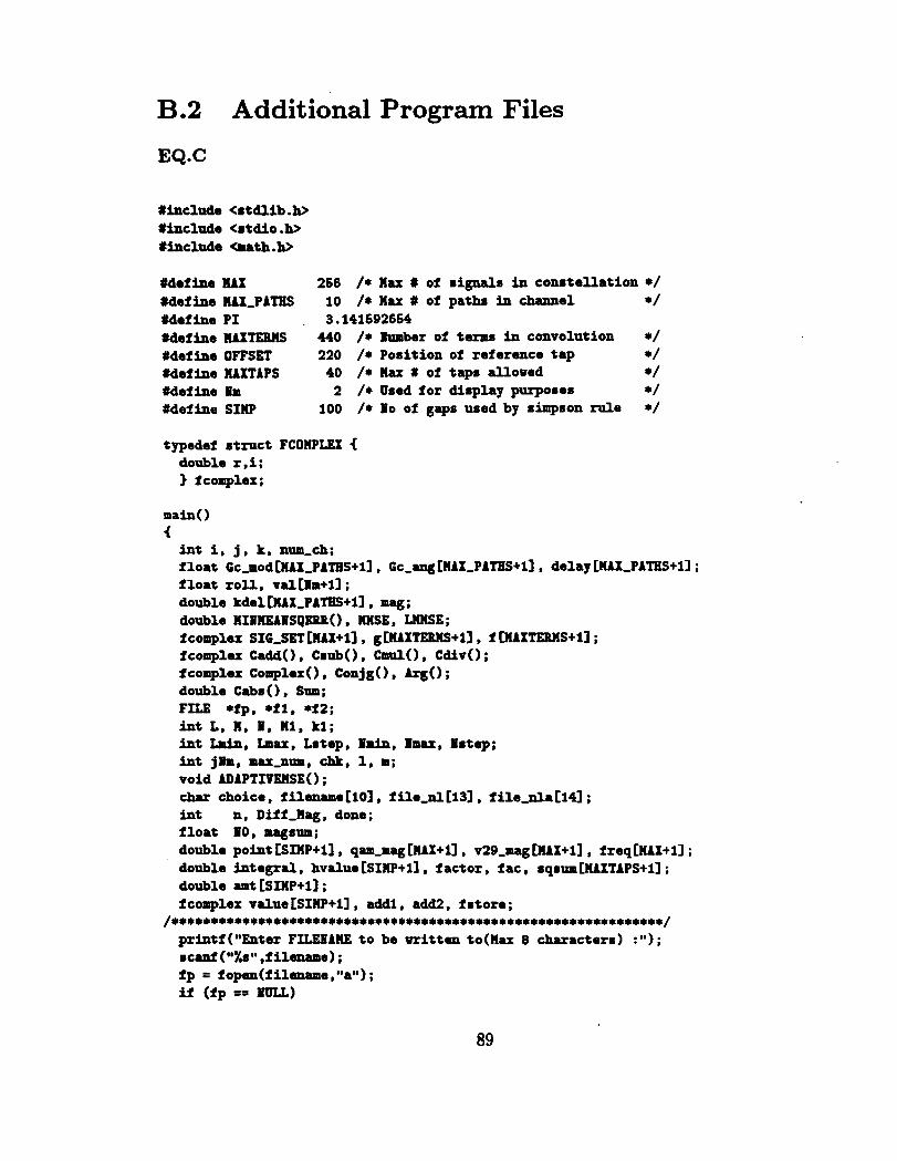
Additional Program Files
#define lux #def ine MAX,PArn #define PI #define HAxmMs #define OFPSEI #def in0 HAXTAPS #define Pm #def ine SIUP
266 /* Hax # of signals in constellation */ 10 /* Hax # of path in channel */ 3.141692664 440 /* number of terms in convolution */ 220 /* Position of reference tap */ 40 /* Hax # of taps allowed */ 2 /* Used for display purposes * /
100 /* Po of gaps used by simpson r u l e */
typedef stmct FCOHPLEX < double r , i ; 1 fcomplex;
main0 < int is j, k, num-ch; float GC-rodCHAX ,PAIES+l] , GC-ang CHAX,PATES+~~ , delay CHAX,PATES+~] ; float roll, val CPm+ll; double kdel [UX,PA?ES+II , mag; double HIPIIEIPSQ~RO, IMSE, LIMSE; I C O ~ ~ ~ O X SIG,SET~HAX+I~ , ~CHAXTERHS+I~ , f IHAX'IEB~S+II ; fcomplex CaddO, CsubO, CnmlO, CdivO; fcomplex ComplexO, ConjgO, k g 0 ; double Cabs ( 1, Sum; FILE *fp, *fl, *f2; int L, H, n, Hl, kl; int Lmin, Lmax, Lstep, Pmin, Pmu, Istep; int jlm, mu-num, chk, 1, a; void ADAPTIVEHSEO ; char choice, f ilename[lOl, f ile,nlC13] , f ile-nlaC141; int n, Diff-Hag, done; float PO, magsum; double point [SIHP+l], qam,mag[HAX+ll, v29,magCHAX+l] , f req[H~~+ll ; double integral, hvalue [SIUP+~] , factor, f ac , sqsm CHAXTAPS+l] ; double amt CSIHP+ll; f complex value CSIHP+l] , add1 , add2, f store;
................................................................. printf ("Enter FILEHAHE to be written to(Hax 8 characters) :@'I ; scmi ("Xs" *filename) ; fp = fopan(filana~e,~a") ; if (fp == am)
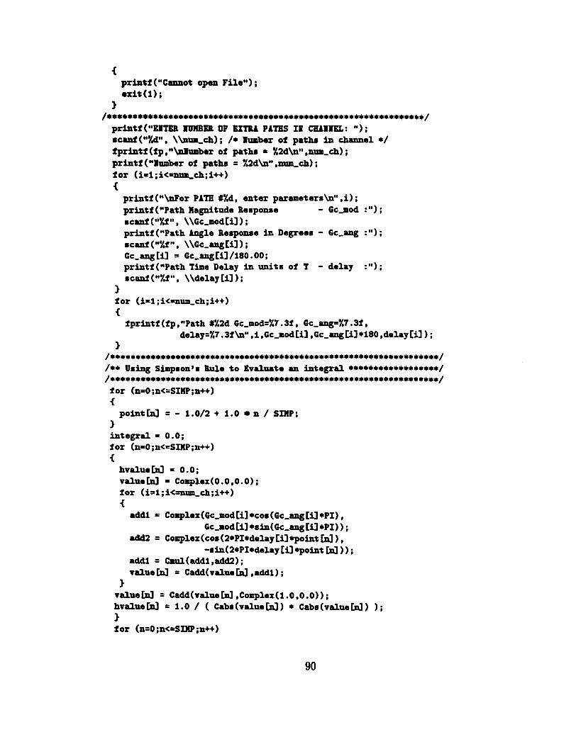
C printf ("Cannot open Filew) ; oxIt(1) ;
1 ................................................................. printf ("EHIEU IUHBEB OF EITFU PATES Ill CHIIPEL : "1 ; 8cmi ("yd" , \bum,ch) ; /* limber of paths in channel */ fprintf (fp ,"bJlumbr of paths = X 2 d W ,n~m,ch) ; printf ("lumber of paths = % 2 d W ,npm,ch) ; for (i=l ; i<=num-ch; i++) < printf ("War PATE #%d, enter parametersW ,i) ; printf ("Path Hagnitude Response - Gc-mod :"I ; ~ca,af(~~?"~~ , \\Gc-modIi1) ; printf ("Path Angle Responre in Degrees - Gc-ang : "1 ; mcanf (aa%f'a, \\Gc,.ng ti1 ; Gc-ang Ci] = Gc-ang ti] /l8O. 00; printf("Path Time Delay in units of T - delay :"I; scanf (*%f " , \\delay ti1 ) ;
1 for (i=l ;i<=num,ch;i++) i f printf (fp , "Path #%2d Gc,mod=%7. Sf, Gc,ang=%7. 3f,
delay=%7.3f \n" ,i ,Gc,modti] ,~c,ang ti] *I80 ,delay ti] 1 ; 3
/** Urimg SiPpson8s Rule to Evaluate an integral ******************/ .................................................................... for (n=O ;n<=SIlIP;n++) i pointkl = - 1.0/2 + 1.0 n / SIHP;
3 integral = 0.0; for (n=O;nc=SIHP;n++) i hvalueCnJ = 0.0; valueCnJ = Complex(O.O,O.O); for (is1 ;i<=num-ch;i++) i add1 = Complex (Gc-mod Cil *cor (Gc-ang Cil *PI) ,
Gc-modCi1 *8in(Gc,angtil *PI) ; add2 = Complex(co8 (2*PI*delay Cil+point CnJ ) ,
-rin(2*PI*delay .point CnJ ) 1 ; add1 = Cmul(add1 ,add2 ) ; value kl = Cadd(value Cnl ,add11 ;
3 valuekl = Cadd(valueCn3 ,Complex(l.O,O.O));
for (n=O;n<=SIlP;n++)
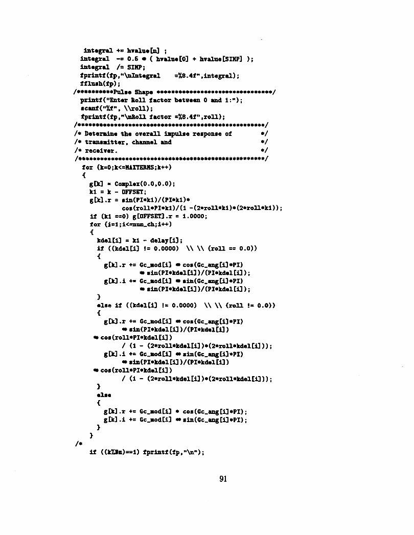
integral += hvalue W ; integral -= 0.5 ( hvalne 101 + hvalne CSIHPI 1 ; integral /= SIWP; fprintf(fpSH\nIntegral =X8.4fu,integral); f f lorh(fp) ;
/**********mre Wp ................................. printf(ooEnter Boll factor betwean 0 and I:"); r~aaf(~Xi~, \\roll); fprintf (fp ,%Roll factor =%8.4f ,roll) ;
...................................................... /* Determine the overall impulse response of */ /* transmitter channel and */ /* receiver. */ ...................................................... for (k=O ; k<=HAXTERHS; k++) < gkl = Complex(O.O,O.O); kl = k - OFFSET; g W .r = rin(PI*kl)/(PI*kl)*
cos (roll*PI*ki)/ (1 -(2*roll*kI )* (2*roll*kl) ) ; if (kl ==O) g [OFFSET] .r = 1.0000 ; for (it1 ; i<=num-ch; i++) < kdel ti] = kl - delay ti] ; if ((kdelCi1 != 0.0000) \\ \\ (roll == 0.0)) < g W .r += Gc-modCi1 cos(Gc,angCil*PI)
rin(PI*kdel ti] )/ (PI*kdel ) ; g W .i += ~c-modCiI rin(Gc-angCi1 *PI)
rin(PI*kdelCil )/(PI*kdel[il) ; 3 else if ((kde1Cil != 0.0000) \\ \\ (roll != 0.0)) i g Ckl .r += ~c-modCi1 cor (Gc,angtil*PI)
rin(PI*kdel Cil ) /(PI*kdel Cil ) cos (roll*PI*kdel Ci] )
/ (I - (2*roll*kdelCil) *(2*roll*kdel till ) ; g W .i += Gc-modci] rin(Gc,angtil*PI)
rin(PI*kdel [ill/ (PI*kdelCil) con (roll*PI*kdel [i] )
/ (I - (2*roll*kdel [ill * (2*roll*Mel Cil ) ) ; 3 0180 < g Ckl .r += Gc-mod ti * con (Gc-ang Cil *PI) ; g lhl .i += Gc-modCi1 sin(Gc,ang Cil *PI) ;
3 3
/* if ((k?"m)==l) fprintf (fp ,"bm) ;
/* Determine receiver response for channel additive noise */ ................................................................... for (k=0 ; k<=lUXTERHS;k++) < k1 = k - OFFSET; f W = Complex(o.o,O.o); if (roll == 0.0) fCOFFSET1.r = 1.0; else < for (i=O;i<=SIHP;i++) amt [il = 0 .O; for (i=O;i<=SIMP;i++) amt Cil = sqrt(1-sin(PI*(2*i/SIHP -1)/2)) ;
/***** 6 ~ - kl ******/ if ((hi != 0) \\ \\ (kl%2 == 0)) i fstore = Complex(0.0,O.O); for (i=O;i<=SMP;i++) f 8tore.r += 2 amt [i] cos(roll*PI*k1*(2*i/SIHP - 1)) ;
f store .r -= (amt [Ol + amt [SIMP] ) * cos (roll*PI*kl ) ; f 8tore.r *= (roll/SIHP/sqrt(2.0) ) ; fCh1.r = sin(kl*PI*(l-roll))/PI/kl + f8tore.r ;
for (i=O;i<=SIHP;i++) fst0re.i += 2 amt[i] sin(roll*PI*kl*(2*i/SIHP - 1));
fst0re.i -= (amt [SIHP] - amt LO]) sin(roll*PI*kl) ; f store. i *= (roll/SIHP/sqrt (2.0) ; f Ckl .i = f8tore.i;
1 /***** odd kl *******/ else if 1 != 0 \\ \\ (klX2 != 0 ) ) < fstore = Complex(O.0,O.O); for (it0 ; i<=SMP ; i++) f8tore.r += 2 * amtCi1 * cos(roll*PI*kl*(2*i/SIIIP - 1));
f store .r -= (amt LO1 + amt CSIHP] ) cor (roll*PI*kl) ; f8tors.r *= (roll/SIllP/sqrt(2.0)); f W . r = sin(kl*PI*(l-roll))/PI/kl - f8tore.r ;
for (i=0; i<=SIHP; i++) f8tore.i += 2 amtCi1 sin(roll*PI*kl*(2*i/SIHP - 1));
f 8tore.i -= (amt [SIHPI - amt CO] ) sin(roll*PI*kl) ; f store. i *= (roll/SIHP/sqrt (2.0) ) ; f W .i -= f8tore.i;
1 else if (kl ==O)
< f a to re = Complex(O.0,O.O); f o r (i=O;i<=SMP;i++)
f8tore . r += 2 * amtCi1; f8tore . r -= (amtCO1 + amtCSIHP1); f r t o r e .r *= (roll/SIHP/sqrt (2 .O) ; fCOFPSEI1.r = 1 - r o l l + f8tore . r ;
3 3
3 f f l run(fp) ;
................................................................... /* Determine the inpat data signals */ /* ith her PSK, qAU, V29 or other, H=2,4,8 ,16,32,64,128,256 */ ...................................................................
f o r (i=0 ; i<=HAX; i++) SIG-SET Cil = Complex (0.0 ,O .o) ; f o r (i=0 ; i*=nAXIAPS ;I++ sqsum [il = 0.0 ; Sum = 0.0; printf("\n VHAT SIGPAL COHStELLATIOP IS DESIBED?bW); pr intf (" Enter P or p(PSK), Q or q(QAH), V or v(V29)"); p r in t f (" or something also b\t : " ) ; .c(LPI("Xs", \\choice) ;
if ((choice == 'p') I I (choice == 'P')) <
printf ("PSK Chosen: How Many Points?: "1; s c d ("Xd" , \\HI ; fpr in t f (fp,"bbXdPSK" ,HI ; f o r (kt1 ;k<=H;k++) C
SIC-SET W .r = con (2*PI*k/H) ; SIG-SETW .i = 8in(2*PI*k/H);
3 3 e l r e i f ((Choica == 'q' ) I I (choice == ~ q ' ) ) i
printf ("QAH chosen: How Many Points? : ") ; .cad (*oXd80 * \\HI ; fpr intf (fp, "bbX2dQAH" , H I ; H i = ( i n t ( f loat h q r t (1 .OO*H) ; f o r (k=O;k<=Hl-1 ;k++) C
f o r (kl=l ;kl<=Hl ;kl++) i
SIG,SETb*Hl+kll .r = (2.0*kl - n l - 1) ; SIG,SEIb*Hl+kll .i = (?.Oak - H i + 1) ; Sum = Sum + SIG,SEICk*Hl+kll .r * SIG~SETCk*Hl+kll .r +
Sf G-SET b*Hl+kll .i SIG-SET b*Hl+kl] . i ; 1
3
printf (%Sum of squares= %8.4fM ,Sum) ; Sum = rqrt(Sum/H); DiifJag = 0; f o r (i=l;i<=HAx;i++) freqCi3 = 0.0; f o r (i=l;i<=HAX;i++) qam,magCil = 0.0; f o r (k=O ;kc=Hl-1; k++) <
fo r (kl=1;kl<=Hl;kl++) <
SIG,SEICk*Hl+kll .r /= Sum; SIG,SEIb*Hl+kI] .i /= Sum; mag = Cabr (SIC-SET tk*Hl+ki] ) ; done = 1; fo r ( i = l ;ic=Diff ,Hag;i++) <
i f (qam-mag Cil == mag) <
f req l i l += 1 .O/H; done = 0;
3 3 i f (done == 1) <
Dif f ,nag++ ; qam-mag CDif f ,Hag1 = mag; f req CDif f , H a g l += 1 . O/H ;
3 3
1 for ( i = l ; i<=Dif f ,Hag; i++) sqsumC11 += f roqCi1 /qam,mag C i l /qam,magCil;
for ( i = l ;i<=Dif f ,Hag;i++) for (j=l;j<=Diff,Hag;j++)
sqsum C2l += f req Cil f reqC jl / (qam-mag C i l qam-mag C jl ) / (qm-mag 111 +qam,mag C jl ;
fo r (i=l;i<=Diff,Hag;i++) for (j=l;j<=Diff,Hag;j++)
for (k=l ;k<=Diff ,Hag; k++) sqsumC31 += freqCi1 * freqCjl * f r e q W
/ (qm-mag Cil +q-aag Cjl +qmmag tkl 1 / (qm-mag Cil +qam~ag C jl +qaPlmag tkl 1 ;
fo r (i=l;i<=Diff,Hag;i++) for (j=l;j<=Diff,Hag;j++)
for (k=l ;k<=Diif ,Hag;k++) for (l=l;l<=Diff,Hag;l++)
for (m=l ;m<=Diff ,Hag;m++) sqrum[61 += freqCil freqCj] * fraq[k] freq[U f r e q m / (qam-mag Cil +qam,mag C jl +qam,mag Ckl +qam,mag CU +qam,mag GIII / (qam-mag 113 +qam,mag C jl +q-,mag tkl +qamBag CU +qmmag LP3 ;
for ( i = l ; i<=Dif f ,Hag; i++)
C f pr intf (f p , "\nQam,Hag= X8.41, Freq = X8.4f1@ , qam-mag Cil , f req Cil ) ;
3 f o r ( i = l ; i<=S;i++) C
if (i!=4) i p r in t f (fp,@@\p.qmum~?"= X8.M '@ ,i ,mqmum~i~ ) ; 3
3 e l s e i f ((choice == 'v') I I (choice == 'v')) C
printf ("V29 chosen: How Hany Points? : "1 ; s c m i (''23" , \\HI ; printf ('@'%d V29 SIGHAL SET" ,H) ; fpr intf ( fp ,"bb%2dV29" ,HI ; H i = H/8; pr intf ( ' @ M i ==%do' ,Hi) ; mag = 1.0; Diff ,Hag = H i 2; f o r (i=0 ; ~ < = H A x ; i++) v29,mag [il = 0.0 ; fo r (i=o;i<=Hl-l;i++) i
j = 8 * i + i ; f o r (k= j ; k<= j+3 ;k++) i
SIC-SETW .r = mag cor(PI*(2*k-11/41; SIG,SETCLJ .i = mag min(PI*(2*k-11/41; Sum = Sum + SIG-SETW .r * SIG-SETW .r
+ SIG-SET W . i SIC-SET W .i ; 3 v29,mag[2+i+ll = mag; mag = mag (2*i+3) / (2*i+1) / sqrt(2.O) ; f o r (k=j+4;k<=j+7;k++) C
SIC-SETW .r = mag com(PI*k/2) ; SIC-SET W .I = mag min(PI*k/2) ; Sum = Sum + SIC-SETW .r SIG-SRbl .r
+ SIG-SET W .i * SIG-SET w .i ; 3 v29,mag C2*i+2l = mag ; mag *= mqrt(2.0);
3 pr intf ("Wum of squarer= %8 .4fN ,Sum) ; Sum = sqrt(Sum/H); f o r (k=l;k<=H;k++) C
SIG-SETCkL'J .r /= Sum; SIG-SETCL'J .i /= Sum;
3 f o r ( i = l ;i<=Dif f ,Hag;i++) v29,magCil /= Sum;
for (i=1 ;i<=Diff,llag;i++) for (j=l;j<=Diff,Hag;j++) sqsrrm121 += 1 .O /(v29,maglil +v29,magCjl)
/ (v29,mag Cil +vzQ,mag C j3 ; for (it1 ;i<=Diff ,Hag;i++) for (j=l;j<=Diff,Hag;j++) for (k=l ;k<=Diff ,Hag;k++)
sqsrrm[3] += 1.0 /(v2Q,mag Cil +v2Q,magC jl +v2Q,magb] ) /(v29,mag 113 +v29,magC jl +v29,mag Ckl ;
for (i=l ; i<=Dif f ,Hag;i++) for (j=l;j<=Diff,Hag;j++) for (k=l ;k<=Diff ,Hag;k++) for (It1 ; l<=Dif f ,Hag ; l++) for (m=l;m<=Diff,Hag;m++) sqrumC61 += 1.0
/ (v29,mag CiJ +v29,mag Cjl +v29,mag bl +v2Q,mag 111 +v29,mag Gal /(v2Q,mag Cil +v29,mag Cjl +v29,mag Ckl +v2Q,mag [lj +v29,mag ) ;
for (i=l;i<=6;i++) sqrum[i] /= pot?( (double) Diff-Hag, (double) i) ;
fprintf (f~,*~b") ; for (i=l;i<=S;i++) fprintf(fp,'%8.1f",pow( (double) Diff-Hag, (double) i));
for (i=l;i<=Diff,Hag;i++) C fprintf (fpt"\nV29,Hag= %8.4f O0 ,v29,mag[il) ;
3 for (i=l;i<=S;i++) C if (i!=4) fprintf(fp.oobqsmD"= %8.4foD,i,sqsmCil);
3 3 else /* AYT MHBR SET */ C printf("\n Enter Ilumber of Points in Signal Constellation:\n"); scanf (oo%do*, \\HI ; f printf (fp ,"\n\nSignal Set not PSK or QAH or V W O ; for (k=l ; k<=H ; k++) < printf ("SICC%dl .r =" ,k) ; scaaf("W .SIG,SETCkl .r) ; printf (ooSIGCLdl .i = O0 ,k) ; ~canf("%f*~ ,SIG,SETM .i) ; Sum = Sum + SIG-SET bl .r SIG-SET Ck] .r +
SIG-SET [L) . i SIC-SET lf'J . i ; 1 printf ( % S u m of squarer = X8 .4fU ,Sum) ; sum = sqrt(Sum) ;
for (kt1 ;k<=H;k++) < SIG-SETW .r /= Sum; SIC-SET El .i /= Sum;
3 3
......................................................................... /**+**+***+*************** Print Corntellation Set ...................... ......................................................................... for (k=l ; k<=H ;k++) < if ((kYJIm) == 1) fprintf(fp,"\n"); fprintf (fp,"srL3d=%8.41,%8.4fj ",k,SIG,SETW .r,SIG,SETbl .i);
3 f f lush(f p) ;
......................................................................... /* What are the step-sizes that are used */ ......................................................................... for (i=O;i<=Ym;i++) val[il= 0 .O; printf ("\prumbar of UPHIS to be entered:"); scanf (*O%do8 , \bax,num) ; for (&=I ;chk<=maxsum;chk++) < printf ("Enter ALPHIrL2dI: " ,chk) ; ~canf(~~W". \\valkhkl);
1 -,
/* Determine loise Power */ ....................................................................... scanf("YJ", \\110); fprintf (fp,"\n\nllO/2= M.41 dBW,11O) ; 110 /= 10.0; 10 = 1.0/p0s(10.0,110) ; f printf (f p. 0'\nl10/2= %8.4f O0 ,110) ; f f lush(f p) ;
. -, /* Determine L and 11 ranges and stepr */ ....................................................................... scanf ( **%doon \\llmin) ; scani ("%d", \\has ) ; scanf(**'M", \\Jistep); sc& (OnYaOO , \\Lmin) ; scanf ( OO%doO , \\Islax) ; ~canf(~~%d~~, \\Lstep) ;
........................................................................ /** Perform Simulations */ ........................................................................ for (I=O ;11<=11max;)l=P+Pstep) <
i
f pr intf ( fp ,"\nbHumber of Equalizer Taps berider C COI = %Idm , I ) ; ff lush(fp) ; WIISE = H I I ~ I S Q ~ ( H , I , S I G , S ~ , g , f ,fp,val,10) ; fprintf ( fp r"\nll=%2d8\tlWSE=X8 .4f\n" ,I ,WIISE) ; f f lruh(fp) ; f o r (L=Lmh;L<=bax ;L=L +Lrtep) <
i f (L != 4) <
fprintf (fp,"\pt = X2d ",L) ; magrum = 0.0; factor = 0.0; fac = 0.0; i f ((choice == 'p') I I (choice == 'P' 1) <
magrum = 1.0 * L; factor = L I0 integral / (m.grum magrum); fac = 1 - (0.6 factor factor) ; LHHSE = 1 - (1-HHSE) fac fac; fprintf (fp8"HHSE=%8.4f" ,tWnSE) ;
3 e l r e i f ((choice == 'q' ) I I (choice == 'Q')) i
factor = L PO integral * rqr~m[L] ; fac = 1 - ( 0 . 5 * f a c t o r * f a c t o r ) ; LHllSE = 1 - (1-IRISE) fac * fac; fprintf (fp , "HHSE=%8.4fW ,WMSE) ;
1 e1.e i f ((choice == ' v ' ) I I (choice == 'V')) i
factor = L 10 integral rqrumCLl ; fac = 1 - (0.6 factor factor) ; LHHSE = 1 - (I-IMSE) fac fac; fpr intf (fp, "HHSE=%8.4f O0 ,LMSE) ;
3 e lse f printf (fp , "\n PBOGBUI SOT AVAILABLE FOB SIGIAL SETw) ; fflruh(fp) ; i f ( I == 8) && (L == 3) i
rcuri ("%rU .f i le-nl) ; f l = fopen(fi1e-nl,"w"); i f (f 1 == IIVLt) printf ("Cannot open Fi lew) ; exi t (1) ; rprintf (f ile-nla, "%r%c", f i l e a , 'a' ) ; f 2 = fopen(fi1e-nlaSMv"); i f (12 == P(ILL) i
printf ("Cannot open File") ; exi t (1) ; 3
............................................................. /********** CIIVO - Taken from: Iumerical Reciper in C ****/ /********** Altered to invert complex matricer *+*I#/ /********** instead of just real matrices *+**/ ............................................................. #include <rtdlib .h> #include <rtdio.h> #include <math .h>
typedef rtr~ct FCOHPLEX C double r , i ; 3 fcomplex;
fcomplex ~add() ,Csub() ,Cmnl() ,Cdiv() , E m ( ) ,Complex() ; double Cabs ( ) ; ............................................... /8888888*88888888 LWKSB ......................
void lubkrb(A,I,indx,b) f complex A CIIAXTAPS+l] D(AXTAPS+l] . bCHAXTAPS+l] ; int I, indxCHAXTAPS+ll; < int i* ii=o* ip, j; fcomplex rum;
for (i=l ; i<=l; i++) C ip = indx ti1 ; rum = b Cipl ; bCip1 = bCi1 ; if (ii) for (j=ii; j<=i-1; j++) sum = Csub(rum,Cmul(ACil Cjl ,bCjl)) ;
else if (Cabr(rum)>0.000) ii= i; b[i] = rum;
3 for (i=n;i>=l;i--1 C rum = blil ;
fo r ( j= i+l ; j<=E; j++) arm = Csub(rum,bul(ACil Cjl ,bCjl)) ; i f ( Cabr(ACil[il) > 0.00) <
bCil = Cdiv(rum,ACiI I i l ) ; 3 e lse b [il =sum;
3 1 ................................................
< int i, imax, j, k; double big, dm, temp; double *vv , *vector ( ; f complex rum, dtm2 , -3; void nrerror( 1, f roe-vector ( ;
vv = vector(1 ,HI; *d = 1.0; f o r (i=l;i<=E;i++) <
big = 0.0; fo r (j=i;jc=n;j++) <
i f ((temp = Cabr(ACi1 Cjl)) > big) big = temp; 3 i f (big == 0.0) nrerror("Singular matrix in routine LUDCIIP"); vvCi1 = 1 .O/big;
3
rum = Cmb(rum,Cmul(ACil W ,Aw Cjl) ) ; rCi1 UI = r=; i f ((durn= wti] Cabs(sum)) >= big) i
b i g = dum; irar = i;
1 1 i f (j!=imax) i
f o r (k=l ;k<=P ;k++) <
dum2 = ACimaxlW; r c i p l t ~ l W = rCj1 W; A C ~ I w = d m ;
1 *d = - (ad); vv C h a d =vv C jl ;
3 inaxcj1 = imax; i f (caba(ACj3 [ j l ) == 0.0) /***** Question **/ <
pr in t f (w\nTIPIfi~d", j ) ; pr in t f (%A = %8.4f+%8.4fj",ACjI Cjl .r,Atj] Cj] .i); A C j ] Cjl .r = ?In; ACj] [j] .i = 0.00;
3 i f (j!=H) i
dum3 = ~omplex(l.O,O.O); dum2 = Cdiv(dum3,ACj~Cj~); f o r ( i= j+ l ; i<=l ; i++) A C i l Cjl = ~ m r r l ( ~ C i 1 Cjl , d m ) ;
3 3 free,vector(w ,l , l ) ;
3 .................................................. /********** matrix Inversion program **********/
void ciav(A,y,P) i c o m p i e ~ A CHAXTAPS+II I~AXTAPS+II , y CHAXTAPS+II [HAXTAPS+II ; int P; <
int i, j , indxCHAXTAPS+lI, k; fcornpie~ ID CHAXTAPS+I~ CHAXTAPS+II . AA CHU(TAPS+II C~AXTAPS+II ; f complex c o l CHAXTAPS+lI ; double d; int jHm;
#def ine HAXS 98 ~ . . . . . . . . . . ~ . . . .
/********* Returns uaif om r.v from 0.0 to 1.0 **+*+*e**/ /********* *********/ /********* From: lumerical Recipes in C . Ch.7 pg.207 *********/ .............................................................. float ran0 ( idum) int *id-; <
static float y, maxran, vCMXS1; float dutn; static int iff=O;
j ; w i p e d int i , k; void arerror ( ;
i f (*idnm < 0 I I i f f ==O) <
i f f = 1; i = 2; do i
k = i; i = i << 1;
1 while ( i ) ; m a x r a n = k; rrand(*idrun) ; *id\llP = 1; f o r (j=i;j<nAXS;j++) d m = rand();
f o r ( j= l ; j<UAXS; j++) vCj1 = r and0 ;
1 j = i + y (MXS -l)/maxran; i f ( ( j > (HAXS-1)) 1 1 ( j < 1) )
nrerr~r(~RABO : THIS CAUUOT UPPm") ; y = vCj1; vCj1 = rand0 ; return(y/maxran) ;
1
#define H i 269200 #define I A l 7141 #define I C l 64773 #def ine Bnl (1 .O/Ul) #define 112 134456 #define I12 8121 #define IC2 28411 #define ~ n 2 (i.o/n2) #define U3 243000 #define 113 4661 #def ine IC3 61349 ..................................................................... /********** rat- a tmifomly distributed r .v from 0.0 t o 1.0 ****/ /********** Set idum t o any negative value t o i n i t i a l i z e or ****/ /********** re in i t ia l ize the sequence. *++*/ /********** From: lumerical Recipe8 in C. Ch.7 pg 210 ****/ ..................................................................... f loa t rani (idrun) int *id= ; <
s t a t i c long i x l , ix2, 1x3; s t a t i c f l o a t r 1981 ; f loa t temp; s t a t i c int iff=O;
j ; void =error( ;
if ( * i b < 0 I I i f f == 0) C
i f f = 1; i x l = (ICl-(*id-)) % Hi; i x i = (IAI*~XI+ICI) % n i ; i.2 = i x l Y, n2; 1x3 = it1 % n3; f o r ( j= i ; j<=97; j++) C
i ~ i = (IAI*IXI+ICI) Y, n i ; ix2 = (IA2*ix2+IC2) % n2; r [jl= (ixi+ix2*RH2)*~1;
1 *ib = 1;
1 i x l = (1~l*ixl+IC1) Y, W 1 ; ix2 = (1~2*ix2+IC2) Y, n2; 1x3 = (IA3*ix3+IC3) % n3; j = 1 + ((97*ix3)/H3) ; i f (j>Q7 I I j <I) nrerror ("RAP1 : This cannot happen" ; temp = rtjl; r [j] = (ixl+ix2*Bn2)*Bnl;
........................................................ /**** Return8 a normally distributed deviate with ****/ /**** zero-mean and unit variance, using ranl (idum)****/ /**** as the source of uniform deviates ***e/
/**** From Pumerical Recipes in C. Ch 7.3 pp.216-7 ****/ , . . . . . . . . . . . . . . . . . . . . . . . . . . . . . . . . . . . . . . . . . . . . . . . . . . . . . ., f loa t gasdev(idum) i n t *idam; C s t a t i c int i se t = 0; s t a t i c f loa t grot ; f loa t fac, r, v l , v2; f loa t ranl ( ;
i f ( i s e t == 0) C /* Ye don't have an deviate handy 80 */
do C
, . .
/** pick two uniform numbers in the square a r t - **/ /** ending from -1 t o +i in each direction **/ /** See i f they are in the unit c i rc le , i f not **/ /** t r y again **/ .................................................... vl = 2.0 * ranl(idum1 - 1.0; v2 = 2.0 ranl(idum1 - 1.0;
r = vl * vl + v2 v2; 3 while (r>= 1.0); fac = mqrt(-P.O*log(r)/r); ...................................................... /** low make the Box-Huller Transformation to get **/ /** two normal deviates. Return one and rave the **/ /** other for the next time. **/ ...................................................... grot = vl fac; ...................................................... /** Set flag. **/ ...................................................... imet = 1; return(v2*fac) ;
3 else
...................................................... /** Ye have an extra deviate handy, so m e t the **/ /** flag, and return the extra deviate. **/ ...................................................... iset = 0; return(gsat) ;
typedef mtruct FCOHPLEX ( double r , i ; 3 fcomplex;
fcomplex Cadd(a,b) fcomplex a,b; i f complex c;
fcomplex Crub(a,b) fcomplex a,b; <
f complex c ;
f complex Cmul(a,b) fcomplex 8,b; < f complex c;
f complex Cdiv (a ,b) fcomplex 8,b; C f complex c ; double r ,don;
if (fabr(b.r) >= faba(b.i)) i r=b.i/b.r; don = b.r + r b.i; c.r = (8.r + r * a.i)/don; c.i = (8.i - r a.r)/dan;
3 elre i r = b.r/ b.i; don = b.i + r b.r; c.r = (a.r * r + a.i)/don; c.i = (a.i * r - a.r)/don;
1 return(c) ;
1
f complex Complex(re ,id double re, im; i f complex c ;
c.r = re; c.i = im; return(c) ;
3
double Cabr(z) f complex 2 ; i
double x, y, a ~ , temp;
x = fabr(2.r); y = fabr(z.i); i f (x==O.O) 8w = y; e l re i f (y==O .O) an8 = x; e l re if (x>y) i
temp = y/x; am = x rqrt(l.O + temp temp);
1 else i
temp = x/y; a m = y sqrt( l .O+ temp* temp);
3 re turdam ;
3
f complex Conjg(z) f complex z ; i
f complex c ;
f complex Csqrt (2) f co~pplex 2 ; i
f complex c; doable X , yr o n r; i f ((z.r == 0.0) \\ \\ (z.i == 0.0)) i
c.r = c . i = 0.0; retrrm(c) ;
3 else i
1 = fabs(2.r); y = fabr(z.i); i f (x >= y) i
r = y/x; o = rqrt(x) * sqrt(O.5*(l.O + rqrt(l.O+r * r ) ) ) ;
3 elae C r = x/y; w = sqrt(y) * aqrt(O.6*(r+sqrt(l.O + r * r)));
3 if (z.r >= 0.0) C c.r = w; c.i = z.i/(2.0 * w);
1 else C c.i = (2.i >= 0) ? P : -w; c.r = z.i /(2.0 * c.i);
3 return(c) ;
3 3
f complex Rcmul(x ,a) double x; fcomplex a; 4
f complex c ; c.r = x a.r; c.i = x a.i; return(c) ;
3
f complex Arg(z) f complex z ; C f complex c; c.r = z.r/Cabs(z) ; c.i = z.i/Caba(z) ; retuxn(c) ;
3
............................................................. /********* Utility program: Pumerical Recipes in C ********/ .............................................................
void nrerror (error-text char error-text 0 ; C void exit0 ;
f printf (at&rr ,"lmrarical Bacip.8 run-time error. . \ll") ; fprintf (rt&rr,n%m\n" ,error,text) ; fprintf (mtderr,". . .now exiting to myatam.. .W) ;
double *vector(nl,nh) int nl. nh; C double *v ;
v= (double * )malloc ( ( w i p e d if ( !v) nrerror return(v-nl) ;
.) (nh-nl+l)*rizeof (double)) ; '("~ocation failure in vector()") ;
void f ree,vector(v ,nl ah) double *v; int nl* nh; C free((char*) (v+nl)) ;
3


![Partial Equalization for MC–CDMA Systems in Non-Ideally ... · complexity linear combining techniques [10]. Following the estimation of the channel-state information (CSI), the](https://img.pdfslide.us/doc/110x75/60473afad90a6f74262c7761/partial-equalization-for-mcacdma-systems-in-non-ideally-complexity-linear.jpg)