Embed Size (px)
Citation preview
Wayne State University
Wayne State University Theses
1-1-2013
Developing A System For Blind Acoustic SourceLocalization And SeparationRaghavendra KulkarniWayne State University,
Follow this and additional works at: http://digitalcommons.wayne.edu/oa_theses
Part of the Acoustics, Dynamics, and Controls Commons
This Open Access Thesis is brought to you for free and open access by DigitalCommons@WayneState. It has been accepted for inclusion in WayneState University Theses by an authorized administrator of DigitalCommons@WayneState.
Recommended CitationKulkarni, Raghavendra, "Developing A System For Blind Acoustic Source Localization And Separation" (2013). Wayne State UniversityTheses. Paper 252.
DEVELOPING A SYSTEM FOR BLIND ACOUSTIC SOURCE LOCALIZATION AND
SEPARATION
by
RAGHAVENDRA KULKARNI
THESIS
Submitted to the Graduate School
of Wayne State University,
Detroit, Michigan
in partial fulfillment of the requirements
for the degree of
MASTER OF SCIENCE
2013
MAJOR: MECHANICAL ENGINEERING
Approved by:
Advisor Date
ii
DEDICATION
I dedicate my thesis research to my parents. Without their understanding, support and patience,
this research would not have been possible.
iii
ACKNOWLEDGMENTS
This thesis would not have been possible without the guidance and the help of several
individuals who in one way or another contributed and extended their valuable assistance in the
preparation and completion of this study. Thank you:
My Advisor, Dr. Sean F. Wu for providing the encouragement to set high goals and the
resources and advice to achieve them;
Dr. Emmanuel Ayorinde and Dr. Wen li for their encouraging words, thoughtful
criticism, and time and attention during busy semesters;
Mr.Srikanth Duraiswamy for his help during the experimental work;
And a special thanks to my friends and my family members, for their continues support
and encouragement.
iv
TABLE OF CONTENTS
DEDICATION ......................................................................................................................................... II
ACKNOWLEDGMENTS ................................................................................................................... III
LIST OF FIGURES ............................................................................................................................. VII
LIST OF TABLES .................................................................................................................................. X
CHAPTER 1 INTRODUCTION ......................................................................................................... 1
1.1 Introduction ............................................................................................................................. 1
1.2 Problem definition .................................................................................................................. 3
1.3 Goals and objectives of the thesis .......................................................................................... 4
1.4 Thesis Organization ................................................................................................................ 5
CHAPTER 2 LITERATURE REVIEW ............................................................................................ 6
2.1 Sound sources localization ..................................................................................................... 6
2.1 (a) Triangulation .................................................................................................................................................. 6 2.1 (b) Beamforming ................................................................................................................................................. 7 2.1 (c) Time reversal ................................................................................................................................................. 7
2.2 Cross-correlation..................................................................................................................... 8
2.3 Auto- correlation ................................................................................................................... 11
CHAPTER 3 SOUND SOURCE LOCALIZATION .................................................................... 13
3.1 Acoustic model based triangulation .................................................................................... 13
3.2 Estimating travel time differences of first arrivals ............................................................ 14
v
3.3 The relative arrival times in auto- and cross-correlation functions ................................. 17
3.3.1. Estimating Nj and Nk .................................................................................................................................... 17 3.3.2. Estimating all the relative arrival times in the ACF and CCF ............................................................... 17
3.4 Error analysis on source localization algorithm [33,35,36]............................................... 19
CHAPTER 4 SOUND SOURCE SEPERATION .......................................................................... 20
4.1 Origin of sound separation problem ................................................................................... 21
4.2 Background Information about some of the Sound separation techniques: ................... 22
4.3 Restriction to the number of sources .................................................................................. 23
4.4 Short time source localization and separation ................................................................... 23
4.4.1 Basic Assumptions and Principles.................................................................................................................. 23 4.4.2 Fourier Transform .......................................................................................................................................... 24 4.4.3 Short Term Fourier Transform ....................................................................................................................... 25 4.4.4 Window Function ........................................................................................................................................... 26 4.4.5 Spectrogram ................................................................................................................................................... 28
4.5 Algorithm for Short time source localization and separation ......................................... 29
CHAPTER 5 EXPERIMENTAL VALIDATION OF SOUND SOURCE LOCALIZATION
AND SEPARATION ............................................................................................................................ 31
5.1 Experimental validation for six-microphone set ................................................................ 31
5.2 Comparison between Cross correlation and Auto correlation: ........................................ 34
5.3 Error analysis for source localization ................................................................................. 36
5.3.1 Error analysis of experimental results ............................................................................................................ 36
5.4 Experimental validation for Source separation: ................................................................ 39
vi
CHAPTER 6 CONCLUSIONS .......................................................................................................... 49
CHAPTER 7 FUTURE WORK ......................................................................................................... 51
REFERENCES ...................................................................................................................................... 52
ABSTRACT ............................................................................................................................................ 57
AUTOBIOGRAPHICAL STATEMENT ........................................................................................ 59
vii
LIST OF FIGURES
Figure 1.1: Simplest mixing model .............................................................................................. 4
Figure: 2.1 Cross- correlations between two channels in an Anechoic Chamber. .................. 9
Figure: 2.2 Cross- correlations between two channels outside an Anechoic Chamber. ....... 10
Figure 2.3 : Signals from Man and Speaker to the receiver in AVNC lab ............................ 11
Figure 4.1: Fourier Transform for sine wave ........................................................................... 25
Figure 4.2: Windowing Functions a) Hamming b) Gaussian c) Hanning d) Rectangular
Window ........................................................................................................................................ 27
Figure 4.3: Example showing the working of a window function .......................................... 28
Figure 4.4: Flow chart for the short-time SLAS algorithm. ................................................... 29
Figure 5.1 Prototype device set model. (a) This device consists of six microphones, a web
camera, a thermometer, and the data acquisition systems. (b) NI-9234 signal acquisition
module. (c) NI USB chassis. ....................................................................................................... 32
Figure 5.2: 3D sonic digitizer model 5230XL ........................................................................... 33
Figure 5.3 (a): Speaker kept at a closer distance to the Microphones with cross-correlation
and Auto-correlation results. ..................................................................................................... 34
Figure 5.3 (b): Speaker kept at a left to the Microphones with cross-correlation and Auto-
correlation results. ...................................................................................................................... 35
viii
Figure 5.3 (c): Speaker kept at a right to the Microphones with cross-correlation and Auto-
correlation results. ...................................................................................................................... 35
Figure 5.3 (d): Speaker kept far away to the Microphones with cross-correlation and Auto-
correlation results. ...................................................................................................................... 36
Figure 5.4: Comparison between Cross-correlation and Auto-correlation ........................... 38
Figure 5.5(a): The dominant sound sources of a man’s voice, white noise , and radio sound
were captured by passive SODAR............................................................................................. 39
Figure 5.5 (b): The time-domain signals and corresponding spectrogram of the Mixed
Signal ............................................................................................................................................ 40
Figure 5.5 (c): The time-domain signals and corresponding spectrogram of the separated
Man’s Voice ................................................................................................................................. 40
Figure 5.5 (d): The time-domain signals and corresponding spectrogram of the separated
Radio Voice .................................................................................................................................. 41
Figure 5.5 (e): The time-domain signals and corresponding spectrogram of the separated
White Noise .................................................................................................................................. 41
Figure 5.6(a): The dominant sound sources of a man’s voice, white noise, and clapping
sound were captured by passive SODAR. ................................................................................ 42
Figure 5.6 (b): The time-domain signals and corresponding spectrogram of the Mixed
Signal ............................................................................................................................................ 43
ix
Figure 5.6 (c): The time-domain signals and corresponding spectrogram of the separated
Man’s Voice ................................................................................................................................. 43
Figure 5.6 (d): The time-domain signals and corresponding spectrogram of the separated
Clap sound ................................................................................................................................... 44
Figure 5.6 (e): The time-domain signals and corresponding spectrogram of the separated
White Noise .................................................................................................................................. 44
Figure 5.7(a): The dominant sound sources of a man’s voice, music, white noise and siren
sound were captured by passive SODAR. ................................................................................ 45
Figure 5.7 (b): The time-domain signals and corresponding spectrogram of the Mixed
Signal ............................................................................................................................................ 46
Figure 5.7 (c): The time-domain signals and corresponding spectrogram of the separated
Man’s Voice ................................................................................................................................. 46
Figure 5.7 (d): The time-domain signals and corresponding spectrogram of the separated
Music ............................................................................................................................................ 47
Figure 5.7 (e): The time-domain signals and corresponding spectrogram of the separated
Siren sound .................................................................................................................................. 47
Figure 5.7 (e): The time-domain signals and corresponding spectrogram of the separated
White Noise .................................................................................................................................. 48
x
LIST OF TABLES
Table 2.1:Comparison between Cross and Auto-correlation .............................................37
1
CHAPTER 1
INTRODUCTION
1.1 Introduction
Human or Animal ears are able to perceive the sound or the direction that a sound is
coming from. The ears can recognize the direction of sound by the combination of different
signals that are arriving at them. For instance, consider a situation in a cocktail party wherein the
person is trying to make an attempt to focus on a single voice among difference conversations
along with some music and background noise. The party effect explains about the focus that one
has on a single person talking and ignoring the mixture of other conversations and background
noise, which are of different frequencies. As mentioned above, human/animal ears have
extraordinary ability that enables them to talk and catch a particular sound at the same time in a
dissonance of different sounds.
Our ears have exceptional ability to catch any type of sound in a disturbed environment.
For example, if we consider cocktail party, we pay attention to a single talker avoiding the
unwanted sources surrounding us. If someone in the party room calls out our name, our ears
immediately switch over to the direction of that sound and respond to it within no time. This is
because it has been found that [1] the acoustic source, on which the human ears concentrate, is
three times louder than the ambient noise. This phenomenon happens irrespective of number of
sources surrounding us, making different sounds simultaneously. The ears can detect all the
sounds of different frequencies. So, it can be stated that the ears act as a Band pass filter and it
can concentrate on one particular sound of any desired frequency ignoring all other sounds. In
general, the auditory system follows three steps in detecting sound:
2
1. It detects the sound above a certain threshold frequency or level.
2. It resolves the sound in to different frequencies bands.
3. Depending on above two points, it calculates the phase and direction of the sound.
After learning about all these capabilities of a human ear, there arises an eagerness to
study about the phenomenon that our ear follows for sound separation.
Considering the case in a cocktail party, we can think of developing a technique to locate
the sources of our choice in any kind of environment. This type of technique can be built using a
number of microphones, data acquisition device and a laptop to see the results. This system can
be used to locate and extract any particular sound from a mixture of different sounds which are
being produced by several other sources simultaneously.
The location of the sources and separation has become an important field in recent years.
With growing population and technology, one needs to cope up with the technology with day to
day basis. There are many cases where the sound source localization and extraction of sound is
used. For example, consider a case in a mob where police officers need to handle such a big
crowd. There is every possibility of gunshots being fired from both the ends. The investigation
then try to track the exact location from where that gunshots were fired. The exact location of
the accident has to be known as to continue with the investigation. The extraction of the sound is
also very important in many cases. Many industries nowadays are using this technique for
quality control inspection on the shop floor by pin pointing the machineries that make more
sound or are less efficient. The above technology is used to remove the back ground noise from
the mixture of different sounds.
3
1.2 Problem definition
In the examples mentioned above regarding Cocktail party, Mob and Industrial
applications, there is a need to detect the sound and extract a particular sound. But in all these
cases, there is no prior knowledge of sources, the sounds or the characteristics of the
surroundings. This method where the sound is extracted without any knowledge is known as
Blind source separation [2, 3, 4, 5]. This is one of the challenging tasks in sound separation. As
mentioned above, there is absolutely no knowledge about the surroundings or the sources. Every
source might produce sound with different amplitude and each receiver or the microphones can
get multiple multipaths from the sources. There might be reverberations, diffractions or sound
reflections that might change the entire situation. The sound might get reflected from a chair,
table, wall etc.
In this thesis a new technology is developed that will enable us to capture the exact
location of multiple sources irrespective of any surroundings. We use a technology called Short-
time source localization and separation to locate the exact locations of the sources and extract the
target acoustic signals from the mixed signals that are measured directly.
4
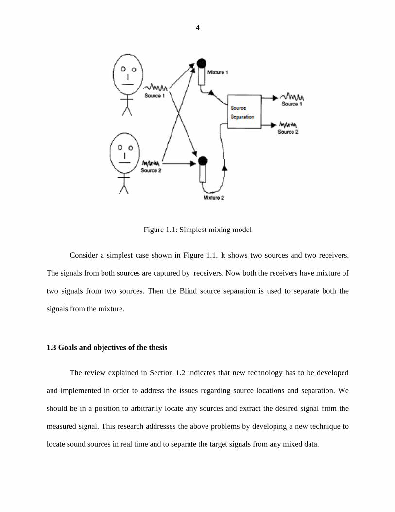
Figure 1.1: Simplest mixing model
Consider a simplest case shown in Figure 1.1. It shows two sources and two receivers.
The signals from both sources are captured by receivers. Now both the receivers have mixture of
two signals from two sources. Then the Blind source separation is used to separate both the
signals from the mixture.
1.3 Goals and objectives of the thesis
The review explained in Section 1.2 indicates that new technology has to be developed
and implemented in order to address the issues regarding source locations and separation. We
should be in a position to arbitrarily locate any sources and extract the desired signal from the
measured signal. This research addresses the above problems by developing a new technique to
locate sound sources in real time and to separate the target signals from any mixed data.
5
1.4 Thesis Organization
The thesis is organized as follows. In chapter 2, we discuss various techniques used for
source localization such the theory of Triangulation, Beam-forming and Time-reversal. Cross-
Correlation, Auto-Correlation functions are also discussed.
In chapter 3, the mathematical formulation to link Auto and Cross correlation are
mentioned which are used to find the accurate source localization. The multipath functions
between the source and the receiver are presented in some detail.
In chapter 4, separation of target sound from directly measured mixed signals is
discussed. A new technology known as Short-time source localization and separation is
discussed along with various concerned parameters such as Fourier transform, Short time
Fourier transform and Window function.
In chapter 5, the experimental validations are carried out in Acoustics, Vibrations and
Noise Control (AVNC) lab, Wayne State University. The source localization is carried out using
Auto Correlation and Cross Correlation functions. Error analysis is performed by comparing the
localization results with the benchmark values obtained from 3-D digitizer. We then carry out the
process for separation of signals using SLAS technique and three different cases are presented
along with their time-domain and Spectrogram graphs.
In chapter 6, we draw conclusions and discuss the significance of the results obtained and
finally in chapter 7, future work that could be carried out in this field is discussed.
6
CHAPTER 2
LITERATURE REVIEW
The algorithms used for source localization used multiple receivers that are microphones
in this thesis. They are used to detect the signal emitted by different sources.
In this thesis, a different approach for source separation is developed, which enables one
to separate mixtures of any type of frequency domain signals. Experimental validations of the
proposed source localization method, source separation are conducted in the Acoustics,
Vibration, and Noise Control (AVNC) laboratory.
2.1 Sound sources localization
There are currently three methodologies developed for the sound source localization
problem, namely, triangulation [6, 7, 8], beamforming [9, 10, 11], and time reversal [12, 13, 14]
algorithms. These methodologies are reviewed below.
2.1 (a) Triangulation
Triangulation is commonly used for source localization and most triangulation
applications are based on intersection of the bearing direction to locate a source on a two-
dimensional plane. It works on an assumption that the sound wave travels between two points in
a straight line. For any impulsive sound source, this method works best in Time difference of
arrival (TDOA) estimation. As the sound wave travels in straight path in an impulse sound, we
get single sharp peak in the cross correlation function. But in case of arbitrary waveforms, where
you have multiple sound reflection and diffraction, this method can’t be used as the number of
peaks in the cross correlation function is more than one. There is no possible way to know which
peak to be used for TDOA estimation unless we use Auto- Correlation functions. The number of
7
sensors needed in this method is typically small compared to other methods.
2.1 (b) Beamforming
Beamforming is a method which assumes that the sound source is at a far distance so that
incident wave front is planar. Beamforming employs delay and sum algorithms to specify the
direction of an incident sound wave travelling in space. This can be explained with an example
of two dimensional array of microphones mounted at a fixed position. The incident sound wave
at an angle impinges on the microphone array. This angle of incidence will produce different
times of arrival (TOA). The signals in all channels are delayed until they are all in phase. These
signals are then summed up to form a peak which gives the source location. The drawback using
this method is that range of a target cannot be determined and also the microphones array has to
be inclined towards the source which needs to be located which is not feasible in all the cases.
2.1 (c) Time reversal
Compared to the above methods, time reversal (TR) method is relatively simple. It
employs a different approach which is playing back the time reversed signals which are emitted
from the same point and then summing them up in space which will lead to the exact source
location. The method is relatively simple and has good applications in the field of underwater
acoustics and reverberant conditions. This method is used whenever the Signal to Noise ratio is
low.
The main disadvantage of TR is that numerical computations are much more time
consuming than the other two methodologies. This is because TR needs to scan every point in
space to find the source.
8
2.2 Cross-correlation
The time delay of a signal between two microphones is the difference between the times
of arrival of the signal at the two microphones. We studied the geometry of the problem by
assuming that we know the time delay of the source between any pair of microphones. Cross
correlation [15, 16, 17, 18] is a routine signal processing technique that can be applied to find
such time delays by using the two copies of a signal registered at a pair of microphones as inputs.
A cross correlation routine outputs set of cross correlation coefficients, which correspond to
different time delays. These coefficients are sum of products of corresponding portions of the
signals, as one signal slides on top of another one. Each cross correlation coefficient corresponds
to a particular possible time delay of a signal between the two microphones. The maximum cross
correlation coefficient indicates the portions of the signals with the maximum correlation.
Therefore, the maximum coefficient can be used to deduce the time delay between the two
copies of the same signal recorded by a pair of microphones. Accurate computation of delay is
the basis for final source location with high accuracy. In the first step, time delay of arrival is
estimated for each pair of microphones.
Assume time domain signals x(t) and y(t) are observed at two measurement positions.
The cross correlation of these two signals Rxy(t) can be expressed as:
dtyxtytxtRxy
(2.1)
where the symbol “ ” indicate the complex conjugate.
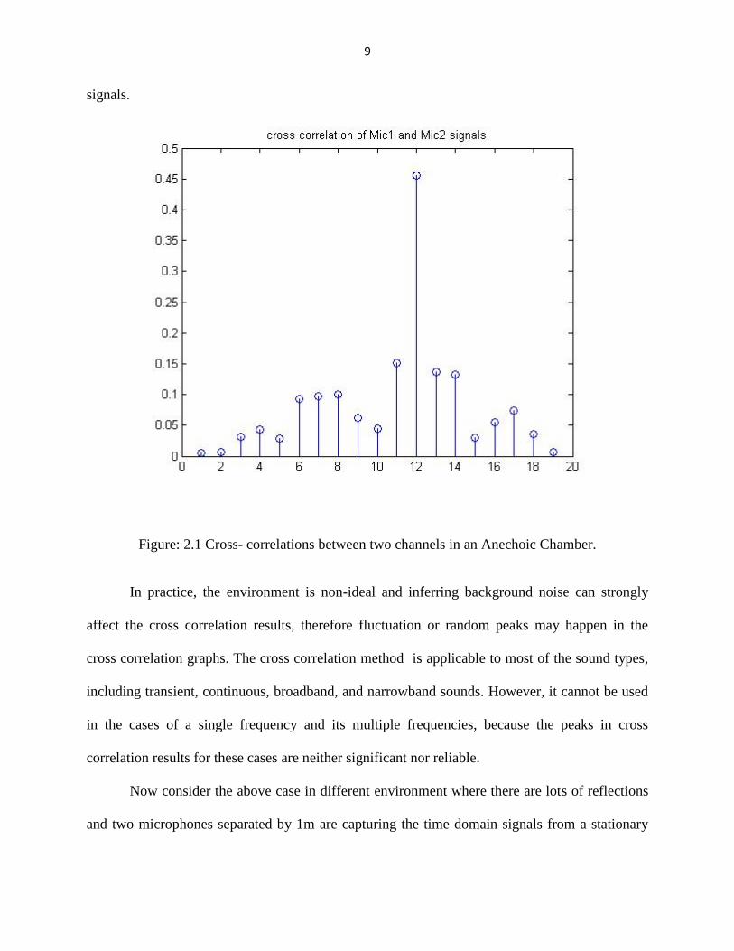
Consider a case in an anechoic chamber with two micro-phones capturing the time
domain signals from two different micro-phones kept at a distance of 1m from each other.
Figure: 2.1 shows the cross-correlation between two microphones that captured the time domain
9
signals.
Figure: 2.1 Cross- correlations between two channels in an Anechoic Chamber.
In practice, the environment is non-ideal and inferring background noise can strongly
affect the cross correlation results, therefore fluctuation or random peaks may happen in the
cross correlation graphs. The cross correlation method is applicable to most of the sound types,
including transient, continuous, broadband, and narrowband sounds. However, it cannot be used
in the cases of a single frequency and its multiple frequencies, because the peaks in cross
correlation results for these cases are neither significant nor reliable.
Now consider the above case in different environment where there are lots of reflections
and two microphones separated by 1m are capturing the time domain signals from a stationary
10
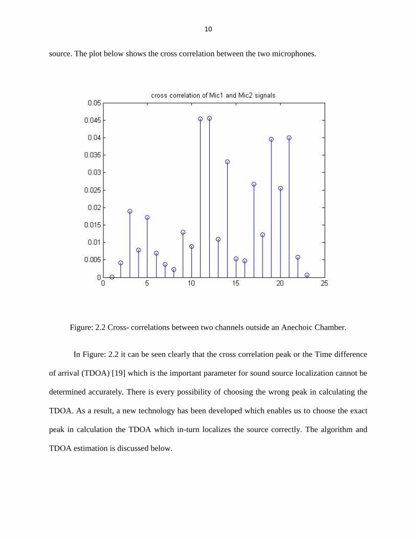
source. The plot below shows the cross correlation between the two microphones.
Figure: 2.2 Cross- correlations between two channels outside an Anechoic Chamber.
In Figure: 2.2 it can be seen clearly that the cross correlation peak or the Time difference
of arrival (TDOA) [19] which is the important parameter for sound source localization cannot be
determined accurately. There is every possibility of choosing the wrong peak in calculating the
TDOA. As a result, a new technology has been developed which enables us to choose the exact
peak in calculation the TDOA which in-turn localizes the source correctly. The algorithm and
TDOA estimation is discussed below.
11
2.3 Auto- correlation
As shown in Figure: 2.2, it is impossible to tell which peak is to be chosen to calculate
the TDOA when the cross correlation is taken between the output of two widely separated
receivers. There might be different multipath [20, 21, 22, 23, 24] with amplitudes which make it
more difficult to choose the exact peak in calculating the TDOA. In such a situation auto-
correlation functions gives sufficient information to identify the relative arrival times of all the
multipaths at each receiver. Cross correlation is used to estimate the arrival time of a signal
between two microphones. However, if there are echoes and reflections which reach the receiver
along with the direct path, there are many peaks in the cross-correlation function
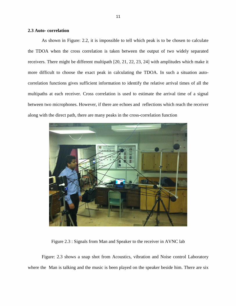
Figure 2.3 : Signals from Man and Speaker to the receiver in AVNC lab
Figure: 2.3 shows a snap shot from Acoustics, vibration and Noise control Laboratory
where the Man is talking and the music is been played on the speaker beside him. There are six
12
microphones which act as receivers and each microphone captures the signals from the Man and
the speaker. For simplicity, only two microphones are shown in the Figure 2.3 receiving the
signals from two sources. Apart from the straight path between the source and receiver, the
signals go through many reverberations and reflections before reaching the receivers. As seen in
the Figure: 2.3, the signal from the Man reached the two Microphones is at different time
interval. Apart from that the Man’s voice reflects from chair, table, glass and the wall and then
reaches the two microphones. Assume same case with the signal from the speaker. If we consider
Microphone 1 and 2, there are three multipaths from Man’s voice to these two speakers.
Therefore the number of cross correlation peaks between these two receivers is 3 x 3 = 9. In
many cases, the first arrival, which may be nearly straight, may be the only useful path for
localization since the geometry of the other paths originating from echoes may be difficult to
estimate. Cross-correlation does not tell us which peak to choose. To address this issue, a new
method is used which identifies the cross-correlation peak corresponding to the difference in
arrival time between the first arrivals at each receiver in the presence of echoes. Its numerical
implementation is efficient. The key to unlocking the multipath problem with cross correlation is
to consider the extra information residing in the reception’s auto-correlationfunctions. They often
provide enough information to identify the relative arrival times of all the multipaths at each
receiver and between receivers.
13
CHAPTER 3
SOUND SOURCE LOCALIZATION
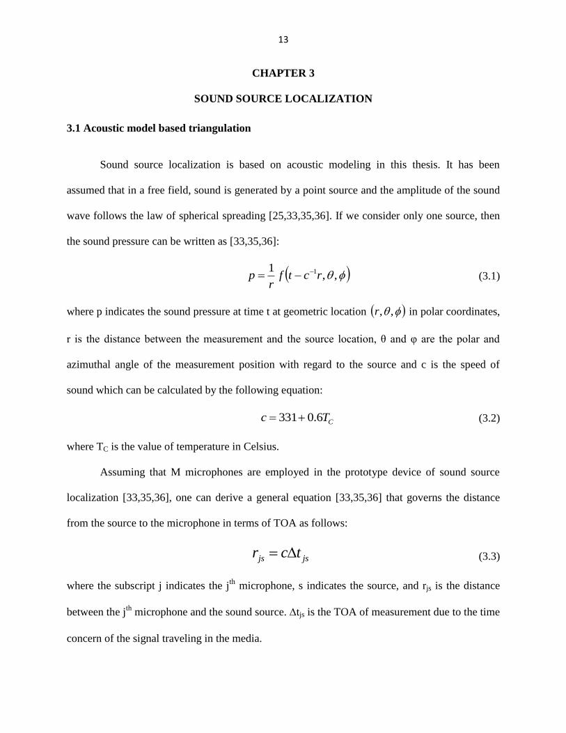
3.1 Acoustic model based triangulation
Sound source localization is based on acoustic modeling in this thesis. It has been
assumed that in a free field, sound is generated by a point source and the amplitude of the sound
wave follows the law of spherical spreading [25,33,35,36]. If we consider only one source, then
the sound pressure can be written as [33,35,36]:
, ,1 1rctfr
p (3.1)
where p indicates the sound pressure at time t at geometric location , ,r in polar coordinates,
r is the distance between the measurement and the source location, θ and φ are the polar and
azimuthal angle of the measurement position with regard to the source and c is the speed of
sound which can be calculated by the following equation:
CTc 6.0331
(3.2)
where TC is the value of temperature in Celsius.
Assuming that M microphones are employed in the prototype device of sound source
localization [33,35,36], one can derive a general equation [33,35,36] that governs the distance
from the source to the microphone in terms of TOA as follows:
jsjs tcr (3.3)
where the subscript j indicates the jth
microphone, s indicates the source, and rjs is the distance
between the jth
microphone and the sound source. tjs is the TOA of measurement due to the time
concern of the signal traveling in the media.
14
Similarly, TOA of the kth
microphone can be written as [33,35,36]:
ksks tcr (3.4)
Using the Equation (3.4) minus Equation (3.3), thus
jsksjsks ttcrr (3.5)
This can be further simplified as:
kijsjs tcrr (3.6)
As mentioned in Chapter 2, it is impractical to model the sound which propagates along
multipath because the environment is poorly known. Cross-correlation between a pair of micro-
phones contain multiple peaks from sources and it is difficult to estimate the time difference of
arrival as the highest peak may not correspond to the difference in path lengths between the
source and the microphones. Hence, a new technology is developed which uses the information
from Auto-correlation function to determine the exact cross correlation peak which will help in
source localization.
3.2 Estimating travel time differences of first arrivals
Consider a source that emits a signal at time zero. Assume the call is described by s(t)
where t is time. Therefore the signal emitted is at t=0. Sound reaches receiver j along paths in
space, called multipaths. The first arrival is often one that does not reflect from boundaries. It
may be the path which most closely approximates the straight line between the source and the
receiver, and thus be useful for localization. The remaining [31] paths reach the
receiver afterward either by undergoing refraction in the medium or by interacting with
boundaries such as chairs, table, walls etc as shown in Figure: 2.3.
15
Assume the pressure field at receiver j is described by
∑
[ ] ( [ ]) (3.7)
where the amplitude and travel time of the nth multipath are [ ], and [ ]respectively. The
noise is [ ].
The autocorrelation function ACF of the signal at channel j is
∫ (3.8)
From Eq: 3.7 and Eq: 3.8 we get,
∑
∑
[ ] [ ]∫ ( [ ]) ( [ ] ) ∫
(3.9)
where the sample ACF between the noise and the signal, that is, ∫ , is assumed to be
negligible [32].
In order to see how to proceed to find the desired arrival time difference, [ ] [ ],
consider the case with three multipaths at each channel j and k. The peaks occur in the
ACF of channels j and k for
[ ] [ ] [ ] (3.10)
[ ] [ ] [ ] (3.11)
[ ] [ ] [ ] (3.12)
And
[ ] [ ] [ ] (3.13)
[ ] [ ] [ ] (3.14)
[ ] [ ] [ ] (3.15)
The peaks in CCF occurs in lags,
16
[ ] [ ] [ ] (3.16)
[ ] [ ] [ ] (3.17)
[ ] [ ] [ ] (3.18)
[ ] [ ] [ ] (3.19)
[ ] [ ] [ ] (3.20)
[ ] [ ] [ ] (3.21)
[ ] [ ] [ ] (3.22)
[ ] [ ] [ ] (3.23)
[ ] [ ] [ ] (3.24)
We can measure any lags that appear in the ACF and CCF, but for which lags do we
know the associated pair of arrival times by inspection? There are four such lags [31, 32].
They are
[ ,1]: the peak with most positive lag in the ACF of channel j. It is due to the arrival
time difference between the first and last multipath.
[ ,1]: the peak with most positive lag in the ACF of channel k. It is due to the
arrival time difference between the first and last multipath.
[1, ]: the peak with most negative lag in the CCF occurs at the arrival time of the
first multipath in channel j minus the arrival time of the last multipath in channel k.
[ ,1]: the peak with most positive lag in the CCF occurs at the arrival time of the last
multipath in channel j minus the arrival time of the first multipath in channel k. The
desired arrival time difference is given by a linear combination of subsets of these four
lags.
17
The desired arrival time difference is given by a linear combination of subsets of these four lags.
3.3 The relative arrival times in auto- and cross-correlation functions
Some or all of the paths of other than the first arrival may sometimes is useful for
localizing signals and mapping the environment with tomography.
3.3.1. Estimating Nj and Nk
The maximum number of peaks [31, 32] in the ACF at positive lag is given by
(3.25)
This does not include the peak at zero lag. If there are less than peaks, then more than
one pair of multipath has similar arrival time differences.
.The lower limit comes from the fact that signals can never yield as many as positively
lagged peaks in the ACF. On the other hand, arrival time degeneracy leads to < .
3.3.2. Estimating all the relative arrival times in the ACF and CCF
The most positively lagged peak in the ACF, , is defined as [ ] [ ]. Now,
peaks require identification in the ACF of channel k. For , the ACF of channel j
has as yet unidentified positively lagged peaks. We need estimates of the following
values of relative arrival times:
[ ] [ ] (3.26)
[ ] [ ] (3.27)
[ ] [ ] (3.28)
[ ] [ ] (3.29)
18
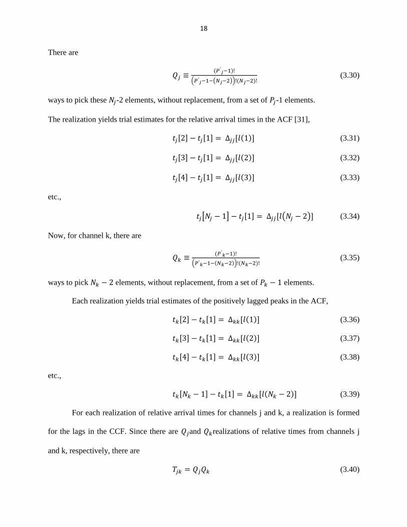
There are
( ( ))
(3.30)
ways to pick these -2 elements, without replacement, from a set of -1 elements.
The realization yields trial estimates for the relative arrival times in the ACF [31],
[ ] [ ] [ ] (3.31)
[ ] [ ] [ ] (3.32)
[ ] [ ] [ ] (3.33)
etc.,
[ ] [ ] [ ( )] (3.34)
Now, for channel k, there are
( )
(3.35)
ways to pick elements, without replacement, from a set of elements.
Each realization yields trial estimates of the positively lagged peaks in the ACF,
[ ] [ ] [ ] (3.36)
[ ] [ ] [ ] (3.37)
[ ] [ ] [ ] (3.38)
etc.,
[ ] [ ] [ ] (3.39)
For each realization of relative arrival times for channels j and k, a realization is formed
for the lags in the CCF. Since there are and realizations of relative times from channels j
and k, respectively, there are
(3.40)
19
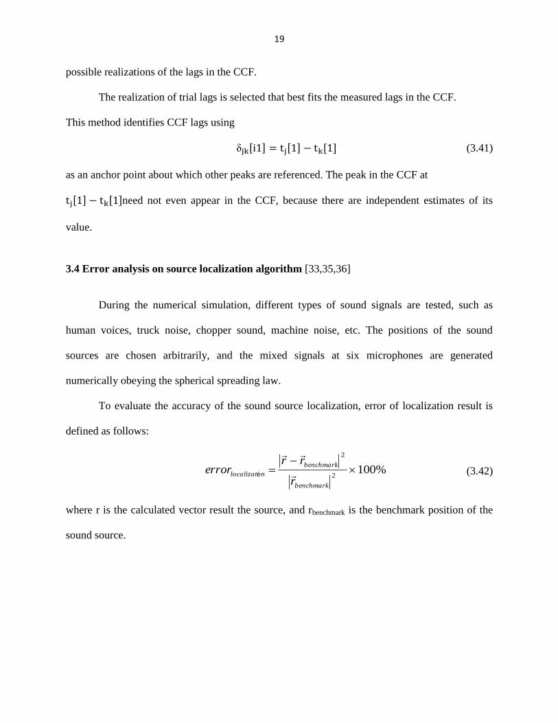
possible realizations of the lags in the CCF.
The realization of trial lags is selected that best fits the measured lags in the CCF.
This method identifies CCF lags using
[ ] [ ] [ ] (3.41)
as an anchor point about which other peaks are referenced. The peak in the CCF at
[ ] [ ]need not even appear in the CCF, because there are independent estimates of its
value.
3.4 Error analysis on source localization algorithm [33,35,36]
During the numerical simulation, different types of sound signals are tested, such as
human voices, truck noise, chopper sound, machine noise, etc. The positions of the sound
sources are chosen arbitrarily, and the mixed signals at six microphones are generated
numerically obeying the spherical spreading law.
To evaluate the accuracy of the sound source localization, error of localization result is
defined as follows:
%1002
2
benchmark
benchmark
onlocalizati
r
rrerror
(3.42)
where r is the calculated vector result the source, and rbenchmark is the benchmark position of the
sound source.
20
CHAPTER 4
SOUND SOURCE SEPERATION
Any unwanted sound is noise and can be produced by many sources like a running
engine, an operating machine tool, man’s vocal cord and so on. Further, quickly varying
pressure wave traveling through a medium is sound and when it travels through air, the
atmospheric pressure varies periodically. Frequency of the sound is the number of pressure
variations per second which is measured in Hertz (Hz) defined as cycles per second. Pitch of
sound wave is directly proportional to the frequency of wave, high frequency wave results in
high pitched sound. Sounds produced by a whistle have much higher frequency than those
produced by drums.
The human ear responds to variations in frequency of sound. The audible range of human
ear falls between 20 Hz to 20 kHz. The human ear is less sensitive to sounds in the low
frequencies compared to the higher frequencies with peak response around 2,500 to 3,000 Hz.
Sound is generally characterized by pitch, loudness and quality. The loudness of a sound
depends on pressure variations. Pressure and pressure variations are expressed in Pascal (Pa). To
express sound or noise in terms of Pa is quite inconvenient because we have to deal with
numbers from as small as 20 to as big as 2,000,000,000. A simpler way is to use a logarithmic
scale. The unit of measurement for loudness is the decibel (dB). As mentioned earlier, the human
ear responds to sound is dependent on the frequency of the sound and this has led to the concept
of weighting scales. The sound pressure levels for the lower frequencies and higher frequencies
are reduced by certain amounts before they are being combined together to give one single sound
pressure level value in a weighting scale. This value is designated as dB(A) and is often used as
it reflects more accurately the frequency response of the human ear. A perceived soft noise has a
21
low dB or dB (A) value and a loud noise has a high one.
4.1 Origin of sound separation problem
Much of the early work in the area of sound recognition and separation can be traced to
problems faced by air traffic controllers in the early 1950's and this effect was first described
(and named) by Colin Cherry in 1953 as part of psychoacoustics [26] . At that time, controllers
received messages from pilots over loudspeakers in the control tower and hearing the intermixed
voices of many pilots over a single loudspeaker made the controller's task of regulation of air
traffic very difficult. Our ability to separate sounds from background noise is based on the
characteristics of the sounds, such as the gender of the speaker, the direction from which the
sound is coming, the pitch, or the speaking speed and this was revealed by Cherry, in 1953, who
conducted perception experiments in which subjects were asked to listen to two different
messages from a single loudspeaker at the same time and try to separate them.
Broadbent, in the 1950’s, concluded that human hearing is basically like a spectrum
analyzer, that is, the ear resolves the spectral content of the pressure wave with respect to the
phase of the signal by conducting dichotic listening experiments where subjects were asked to
hear and separate different speech signals presented to each ear simultaneously (using
headphones). The difference in sound between the ears is a notable exception that provides a
significant part of the directional sensation of sound and is called inter-aural phase difference.
22
4.2 Background Information about some of the Sound separation techniques:
Source separation has long been a topic of interest in engineering and many algorithms
have been developed to perform separation of the sound sources. In 1994, the formulation of a
sound separation technique known as Blind source separation (BSS) by Comon came into
picture. Independent component analysis (ICA) was the name given to the algorithms that were
developed to conduct the source separation. To highlight the fact that independent components
were being separated from mixtures of signals the separation techniques were named ICA and
also to emphasize a close link with the classical signal processing technique of Principal
Component Analysis (PCA).
There was a rapid development of ICA algorithms following the Comon’s seminal paper.
Based on a wide variety of principles algorithms were formulated, including mutual information,
maximum likelihood and higher order statistics, to name just a few of the more popular
approaches. All ICA algorithms are fundamentally similar despite such wide variety. ICA
algorithms invariably obtain estimates of the independent signals by adopting a numerical
approach (e.g. gradient descent) of maximizing an “independence metric”, i.e. a measure of the
signals’ independence.
There came many different approaches to solving the source separation problem with the
explosion of interest of many researchers in BSS and a great deal of progress has been made in
showing that seemingly unrelated approaches were, in fact, equivalent. A major contribution to
this movement was made by Bell and Sejnowski, by proposing a unifying framework for BSS
based on information theoretic considerations [1] . BSS researchers soon showed the equivalence
of many different approaches to BSS by continuing on the work of Bell and Sejnowski and
research led to a convergence onto a small set of well understood principles, as the field of Blind
23
Source Separation matured.
4.3 Restriction to the number of sources
Consider situations in which a number of sources emitting signals which interfere with
one another occur, like a crowded room with many people speaking at the same time, interfering
electromagnetic waves from mobile phones or crosstalk from brain waves originating from
different areas of the brain. In each of these situations the mixed signals are often
incomprehensible and it is of interest to separate the individual signals when the total number of
inherent signals are not known to us. No prior information is known about the number of the
source signals that are present but the Blind Source Separation can be used to separate these
signals and so the algorithm for independent component analysis fails and we need to come up
with a modification to the existing algorithm to separate unknown number of sources using a
fixed number of sensors. A successful separation of mixed signals resulted only when the
number of signals is same as the number of sensors, by using the time domain algorithms
proposed by BSS. But, they become inefficient when the number of sources increases then the
sensors. Thus, in this thesis by working in the frequency domain [27], we have proposed an
improved source separation approach.
4.4 Short time source localization and separation
4.4.1 Basic Assumptions and Principles
As depicted in Chapter 3, a source localization technique using Auto and Cross-
correlation which can only locate the most dominant sound source in a specific frequency band
at a specific time instance. Since in general the sound signals are arbitrary, the most dominant
24
signals in different frequency bands at different time instances may be different and this offers an
opportunity for us to separate individual source signals by dividing the time-domain signals into
many short time segments. In general, the shorter the time segments are, the more accurately the
variations in the time-domain signals can be captured, but the worse the frequency resolution in
source separation becomes and this phenomenon is exactly the same as that in short-time Fourier
transform (STFT). To ensure an optimal resolution for both time and frequency in sources
localization and separation, a compromise must be made. However, in this study, STFT is
performed on each time segment, and the resultant spectrum is expressed in the standard octave
bands where by the time-domain signals are divided into a uniform segment of Dt = 0.1 (sec).
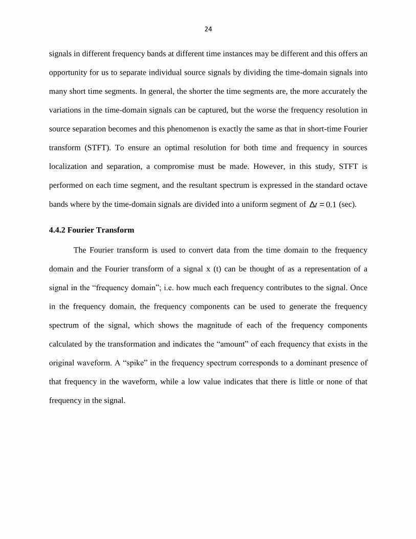
4.4.2 Fourier Transform
The Fourier transform is used to convert data from the time domain to the frequency
domain and the Fourier transform of a signal x (t) can be thought of as a representation of a
signal in the “frequency domain”; i.e. how much each frequency contributes to the signal. Once
in the frequency domain, the frequency components can be used to generate the frequency
spectrum of the signal, which shows the magnitude of each of the frequency components
calculated by the transformation and indicates the “amount” of each frequency that exists in the
original waveform. A “spike” in the frequency spectrum corresponds to a dominant presence of
that frequency in the waveform, while a low value indicates that there is little or none of that
frequency in the signal.
25
Figure 4.1: Fourier Transform for sine wave
4.4.3 Short Term Fourier Transform
A Fourier-related transform used to determine the sinusoidal frequency and phase content
of local sections of a signal as it changes over time is called the short-time Fourier transform
(STFT), or alternatively short-term Fourier transform. This is simply described, in the
continuous-time case, that the function to be transformed is multiplied by a window function
which is nonzero for only a short period of time. The Fourier transform (a one-dimensional
function) of the resulting signal is taken as the window is slid along the time axis, resulting in a
two-dimensional representation of the signal. Mathematically, this is written as:
{ } ∫
(4.1)
where w(t) is the window function centered around zero, and x(t) is the signal to be transformed.
X( ,ω) is essentially the Fourier Transform of x(t)w(t- ), a complex function representing the
phase and magnitude of the signal over time and frequency. The data to be transformed could be
broken up into chunks or frames (which usually overlap each other) in the discrete time case and
each chunk is Fourier transformed [29], and the complex result is added to a matrix, which
records magnitude and phase for each point in time and frequency. This can be
expressed as:
{ } ∫ [ ]
(4.2)
26
In this case, m is discrete and ω is continuous. Again, the discrete-time index m is
normally considered to be "slow" time and usually not expressed in as high resolution as time n.
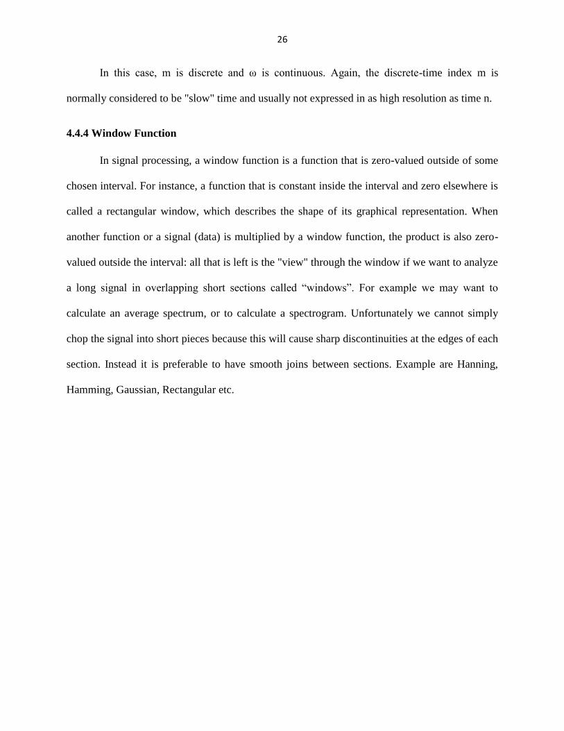
4.4.4 Window Function
In signal processing, a window function is a function that is zero-valued outside of some
chosen interval. For instance, a function that is constant inside the interval and zero elsewhere is
called a rectangular window, which describes the shape of its graphical representation. When
another function or a signal (data) is multiplied by a window function, the product is also zero-
valued outside the interval: all that is left is the "view" through the window if we want to analyze
a long signal in overlapping short sections called “windows”. For example we may want to
calculate an average spectrum, or to calculate a spectrogram. Unfortunately we cannot simply
chop the signal into short pieces because this will cause sharp discontinuities at the edges of each
section. Instead it is preferable to have smooth joins between sections. Example are Hanning,
Hamming, Gaussian, Rectangular etc.
27
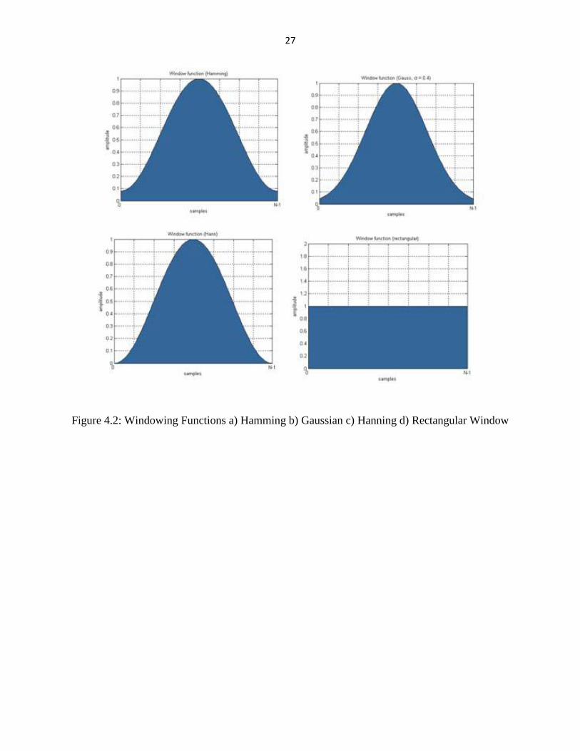
Figure 4.2: Windowing Functions a) Hamming b) Gaussian c) Hanning d) Rectangular Window
28
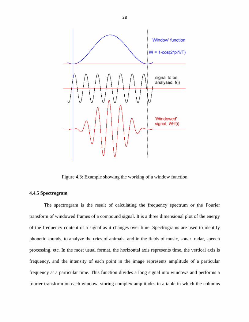
Figure 4.3: Example showing the working of a window function
4.4.5 Spectrogram
The spectrogram is the result of calculating the frequency spectrum or the Fourier
transform of windowed frames of a compound signal. It is a three dimensional plot of the energy
of the frequency content of a signal as it changes over time. Spectrograms are used to identify
phonetic sounds, to analyze the cries of animals, and in the fields of music, sonar, radar, speech
processing, etc. In the most usual format, the horizontal axis represents time, the vertical axis is
frequency, and the intensity of each point in the image represents amplitude of a particular
frequency at a particular time. This function divides a long signal into windows and performs a
fourier transform on each window, storing complex amplitudes in a table in which the columns
29
represent time and the rows represent frequency.
4.5 Algorithm for Short time source localization and separation [34]
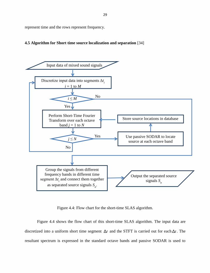
Figure 4.4: Flow chart for the short-time SLAS algorithm.
Figure 4.4 shows the flow chart of this short-time SLAS algorithm. The input data are
discretized into a uniform short time segment Dt and the STFT is carried out for each Dt . The
resultant spectrum is expressed in the standard octave bands and passive SODAR is used to
Input data of mixed sound signals
Use passive SODAR to locate
source at each octave band
Yes
No
Store source locations in database
Output the separated source
signals Sn
Discretize input data into segments Δt
i
i = 1 to M
Perform Short-Time Fourier
Transform over each octave
band j = 1 to N
i ≤ M
j ≤ N Yes
No
Group the signals from different
frequency bands in different time
segment Δti and connect them together
as separated source signals Sn.
30
determine the locations of the dominant source in each band. These steps are repeated until
source localizations in all frequency bands for all time segments are completed. Next, all signals
in various frequency bands at different time segments that correspond to the same source are
strung together, which represent the separated signals. These separated signals may be played
back in which the interfering signals including background noise are minimized.
Theoretically, one may use a much finer resolution in frequency to locate and separate
source signals. For example, for this short time segment Dt = 0.1, one can get a frequency
resolution of Df ³1 Dt = 5Hz. However; this will substantially increase the computation time
because source localization must be carried out over every 5 Hz for every 0.1 second of input
data. For most applications such a fine resolution in frequency is unnecessary. Therefore in this
study the standard octave bands over the frequency range of 20 – 20,000 Hz are used.
31
CHAPTER 5
EXPERIMENTAL VALIDATION OF SOUND SOURCE LOCALIZATION AND
SEPARATION
Validation of Sound source localization using Auto-Correlation is conducted with various
real world sounds in several non-ideal environments. The tests were conducted in Acoustic,
Vibration, and Noise Control Laboratory (AVNC Lab), Wayne State University. Different types
of sounds were used through the speakers and were located through the newly developed code.
Sounds such as music, radio, people talk, clapping etc were used. The experimental validation
was conducted to compare the results between Cross correlation and Auto correlation results to
locate single and multiple sources.
5.1 Experimental validation for six-microphone set
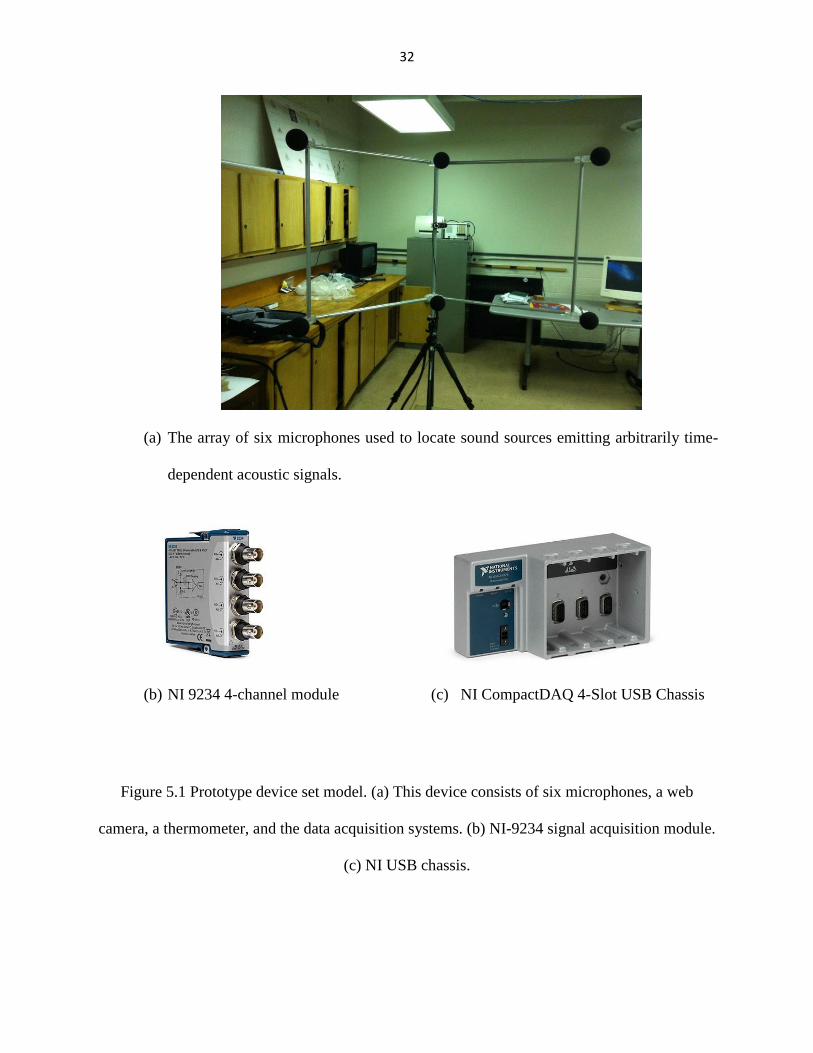
A prototype based on this technology has been developed and its hardware includes six
B&K ¼-in condenser microphones, Type 4935,two 4-channel data acquisition units, Type NI-
9234 ,with a maximum sampling rate of 51.2 kS/sper channel one NI-cDAQ9174 chassis, a
thermometer to measure the air temperature, camera to view the relative positions of located
sources, and a laptop to control data acquisition and post processing.
32
(a) The array of six microphones used to locate sound sources emitting arbitrarily time-
dependent acoustic signals.
(b) NI 9234 4-channel module (c) NI CompactDAQ 4-Slot USB Chassis
Figure 5.1 Prototype device set model. (a) This device consists of six microphones, a web
camera, a thermometer, and the data acquisition systems. (b) NI-9234 signal acquisition module.
(c) NI USB chassis.
33
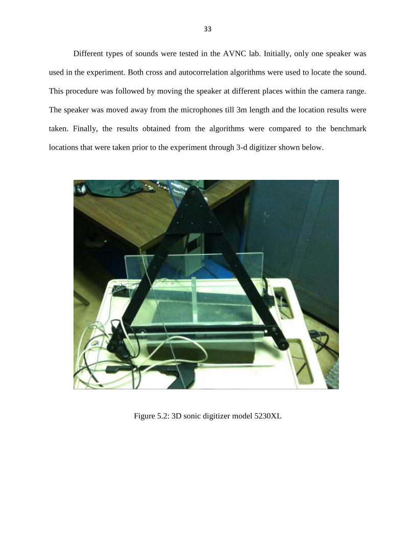
Different types of sounds were tested in the AVNC lab. Initially, only one speaker was
used in the experiment. Both cross and autocorrelation algorithms were used to locate the sound.
This procedure was followed by moving the speaker at different places within the camera range.
The speaker was moved away from the microphones till 3m length and the location results were
taken. Finally, the results obtained from the algorithms were compared to the benchmark
locations that were taken prior to the experiment through 3-d digitizer shown below.
Figure 5.2: 3D sonic digitizer model 5230XL
34
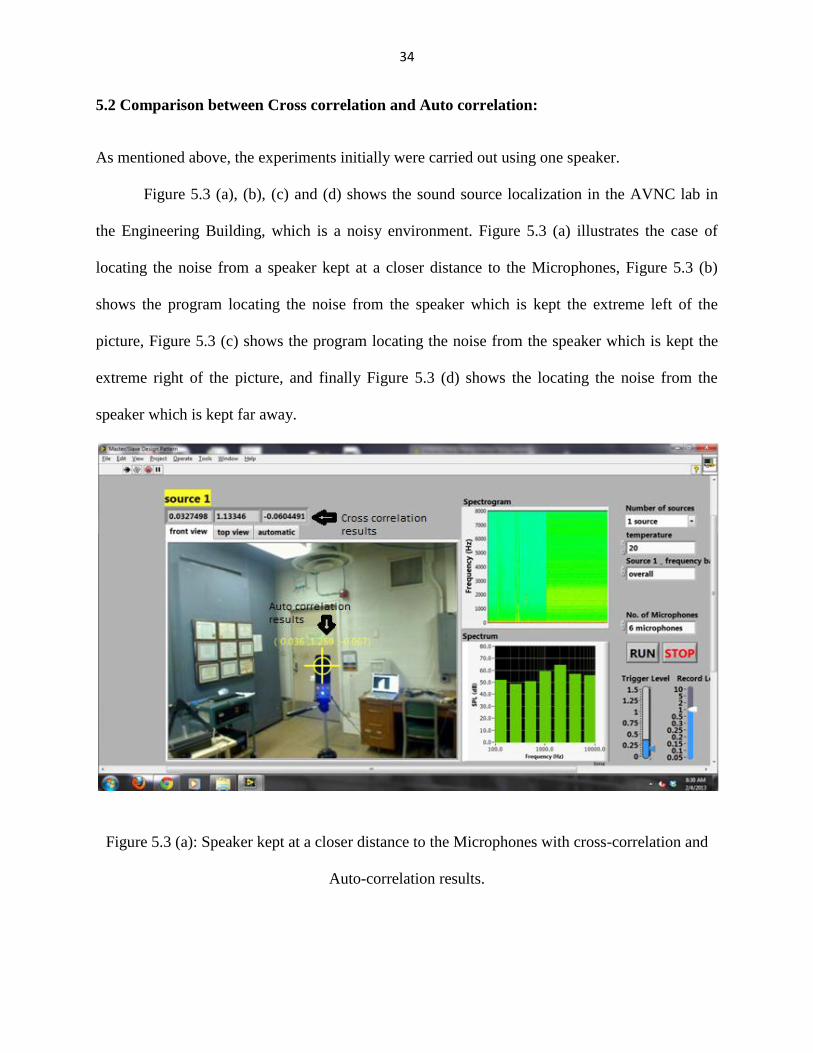
5.2 Comparison between Cross correlation and Auto correlation:
As mentioned above, the experiments initially were carried out using one speaker.
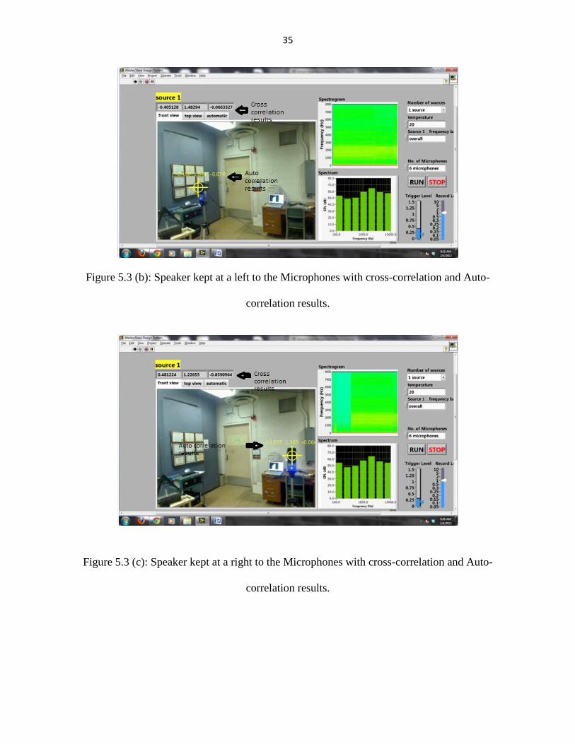
Figure 5.3 (a), (b), (c) and (d) shows the sound source localization in the AVNC lab in
the Engineering Building, which is a noisy environment. Figure 5.3 (a) illustrates the case of
locating the noise from a speaker kept at a closer distance to the Microphones, Figure 5.3 (b)
shows the program locating the noise from the speaker which is kept the extreme left of the
picture, Figure 5.3 (c) shows the program locating the noise from the speaker which is kept the
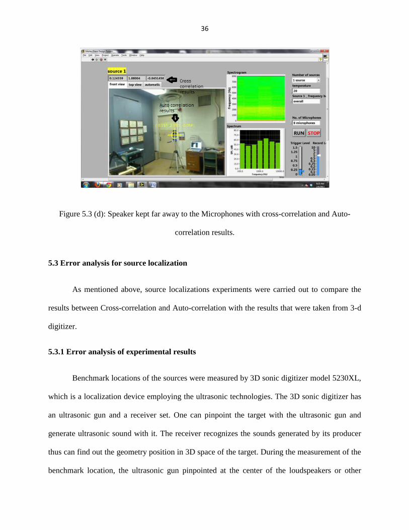
extreme right of the picture, and finally Figure 5.3 (d) shows the locating the noise from the
speaker which is kept far away.
Figure 5.3 (a): Speaker kept at a closer distance to the Microphones with cross-correlation and
Auto-correlation results.
35
Figure 5.3 (b): Speaker kept at a left to the Microphones with cross-correlation and Auto-
correlation results.
Figure 5.3 (c): Speaker kept at a right to the Microphones with cross-correlation and Auto-
correlation results.
36
Figure 5.3 (d): Speaker kept far away to the Microphones with cross-correlation and Auto-
correlation results.
5.3 Error analysis for source localization
As mentioned above, source localizations experiments were carried out to compare the
results between Cross-correlation and Auto-correlation with the results that were taken from 3-d
digitizer.
5.3.1 Error analysis of experimental results
Benchmark locations of the sources were measured by 3D sonic digitizer model 5230XL,
which is a localization device employing the ultrasonic technologies. The 3D sonic digitizer has
an ultrasonic gun and a receiver set. One can pinpoint the target with the ultrasonic gun and
generate ultrasonic sound with it. The receiver recognizes the sounds generated by its producer
thus can find out the geometry position in 3D space of the target. During the measurement of the
benchmark location, the ultrasonic gun pinpointed at the center of the loudspeakers or other
37
sound sources, generated ultrasonic sound, and the position can be obtained by the 3D sonic
digitizer program. For an object within a radius of 4 meters, the error margin of this 3D sonic
digitizer is ±2.5mm. As the localization error of the 3D digitizer is much less than the expected
error of the present approach, the location gained by 3D digitizer can be considered as
benchmark position.
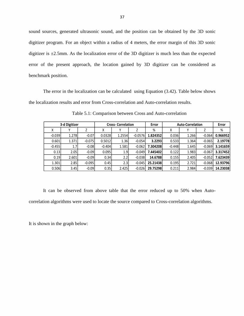
The error in the localization can be calculated using Equation (3.42). Table below shows
the localization results and error from Cross-correlation and Auto-correlation results.
Table 5.1: Comparison between Cross and Auto-correlation
It can be observed from above table that the error reduced up to 50% when Auto-
correlation algorithms were used to locate the source compared to Cross-correlation algorithms.
It is shown in the graph below:
3-d Digitizer Cross- Correlation Error Auto-Correlation Error
X Y Z X Y Z % X Y Z %
-0.039 1.278 -0.07 0.0328 1.2554 -0.0576 1.824352 0.036 1.266 -0.064 0.966952
0.601 1.371 -0.075 0.5012 1.36 -0.054 3.2293 0.533 1.364 -0.065 2.19778
-0.455 1.7 -0.08 -0.404 1.581 -0.062 7.304208 -0.448 1.645 -0.069 3.141659
0.13 2.05 -0.09 0.095 1.9 -0.049 7.445402 0.122 1.983 -0.067 3.317452
0.19 2.601 -0.09 0.34 2.2 -0.038 14.6788 0.155 2.405 -0.052 7.623439
1.301 2.85 -0.095 0.45 2.3 -0.045 25.21438 0.195 2.721 -0.068 12.93796
0.506 3.45 -0.09 0.35 2.425 -0.026 29.75298 0.211 2.984 -0.039 14.23038
38
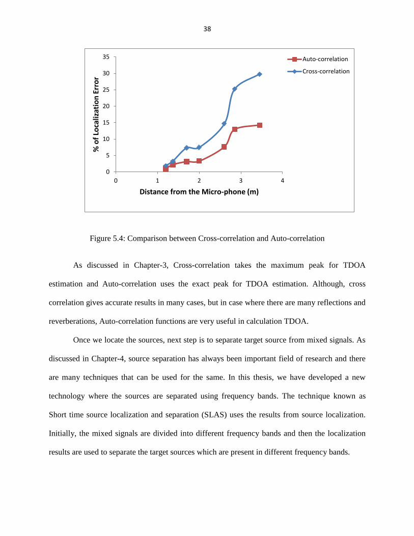
Figure 5.4: Comparison between Cross-correlation and Auto-correlation
As discussed in Chapter-3, Cross-correlation takes the maximum peak for TDOA
estimation and Auto-correlation uses the exact peak for TDOA estimation. Although, cross
correlation gives accurate results in many cases, but in case where there are many reflections and
reverberations, Auto-correlation functions are very useful in calculation TDOA.
Once we locate the sources, next step is to separate target source from mixed signals. As
discussed in Chapter-4, source separation has always been important field of research and there
are many techniques that can be used for the same. In this thesis, we have developed a new
technology where the sources are separated using frequency bands. The technique known as
Short time source localization and separation (SLAS) uses the results from source localization.
Initially, the mixed signals are divided into different frequency bands and then the localization
results are used to separate the target sources which are present in different frequency bands.
0
5
10
15
20
25
30
35
0 1 2 3 4
% o
f Lo
caliz
atio
n E
rro
r
Distance from the Micro-phone (m)
Auto-correlation
Cross-correlation
39
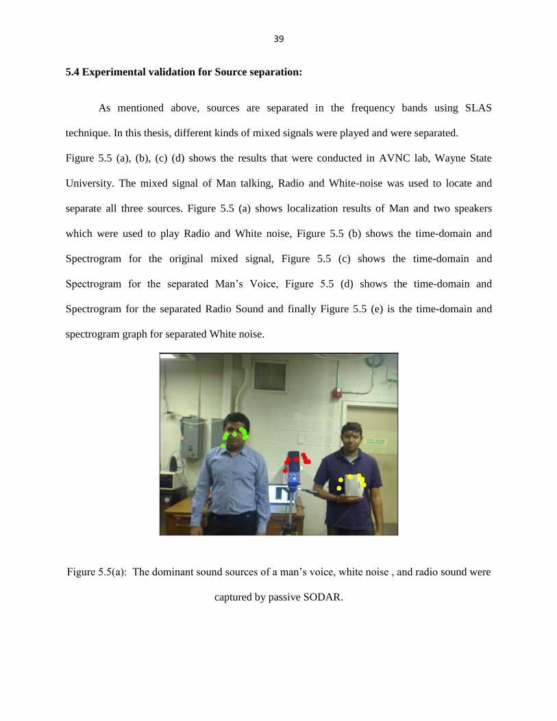
5.4 Experimental validation for Source separation:
As mentioned above, sources are separated in the frequency bands using SLAS
technique. In this thesis, different kinds of mixed signals were played and were separated.
Figure 5.5 (a), (b), (c) (d) shows the results that were conducted in AVNC lab, Wayne State
University. The mixed signal of Man talking, Radio and White-noise was used to locate and
separate all three sources. Figure 5.5 (a) shows localization results of Man and two speakers
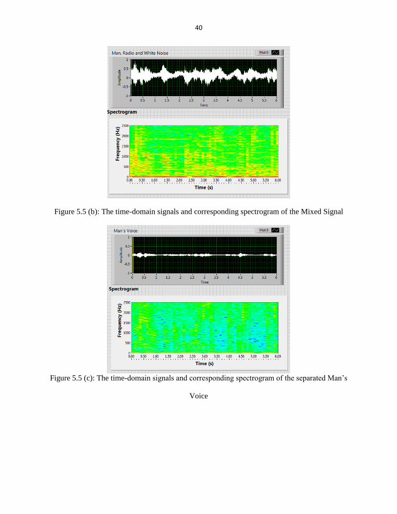
which were used to play Radio and White noise, Figure 5.5 (b) shows the time-domain and
Spectrogram for the original mixed signal, Figure 5.5 (c) shows the time-domain and
Spectrogram for the separated Man’s Voice, Figure 5.5 (d) shows the time-domain and
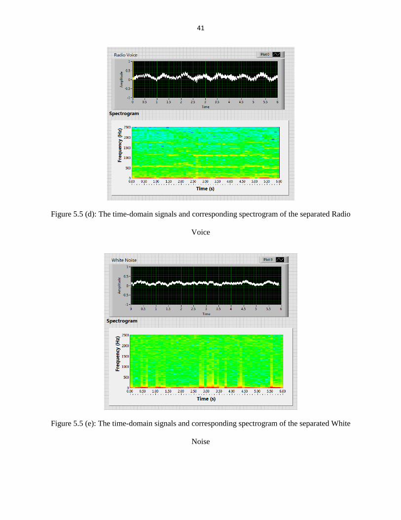
Spectrogram for the separated Radio Sound and finally Figure 5.5 (e) is the time-domain and
spectrogram graph for separated White noise.
Figure 5.5(a): The dominant sound sources of a man’s voice, white noise , and radio sound were
captured by passive SODAR.
40
Figure 5.5 (b): The time-domain signals and corresponding spectrogram of the Mixed Signal
Figure 5.5 (c): The time-domain signals and corresponding spectrogram of the separated Man’s
Voice
41
Figure 5.5 (d): The time-domain signals and corresponding spectrogram of the separated Radio
Voice
Figure 5.5 (e): The time-domain signals and corresponding spectrogram of the separated White
Noise
42
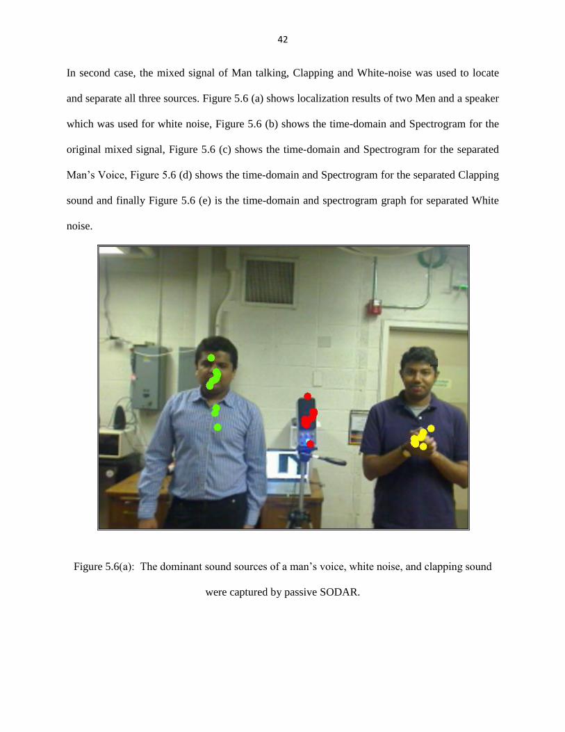
In second case, the mixed signal of Man talking, Clapping and White-noise was used to locate
and separate all three sources. Figure 5.6 (a) shows localization results of two Men and a speaker
which was used for white noise, Figure 5.6 (b) shows the time-domain and Spectrogram for the
original mixed signal, Figure 5.6 (c) shows the time-domain and Spectrogram for the separated
Man’s Voice, Figure 5.6 (d) shows the time-domain and Spectrogram for the separated Clapping
sound and finally Figure 5.6 (e) is the time-domain and spectrogram graph for separated White
noise.
Figure 5.6(a): The dominant sound sources of a man’s voice, white noise, and clapping sound
were captured by passive SODAR.
43
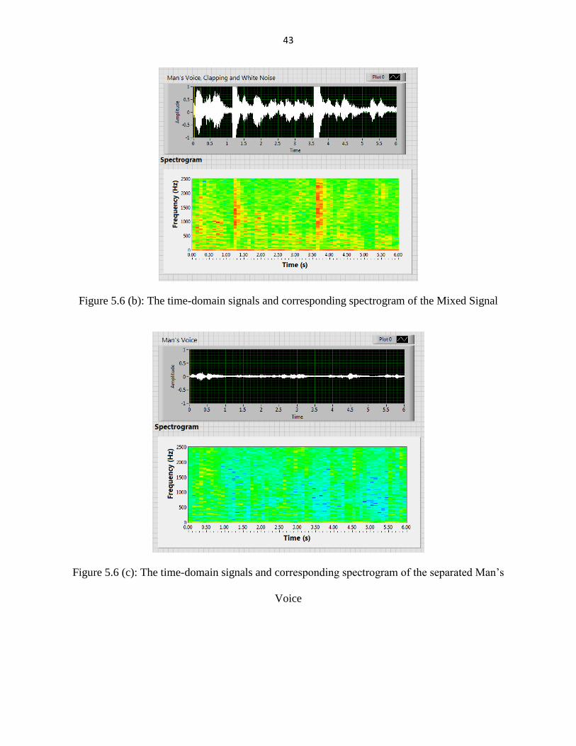
Figure 5.6 (b): The time-domain signals and corresponding spectrogram of the Mixed Signal
Figure 5.6 (c): The time-domain signals and corresponding spectrogram of the separated Man’s
Voice
44
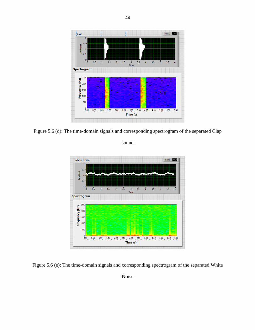
Figure 5.6 (d): The time-domain signals and corresponding spectrogram of the separated Clap
sound
Figure 5.6 (e): The time-domain signals and corresponding spectrogram of the separated White
Noise
45
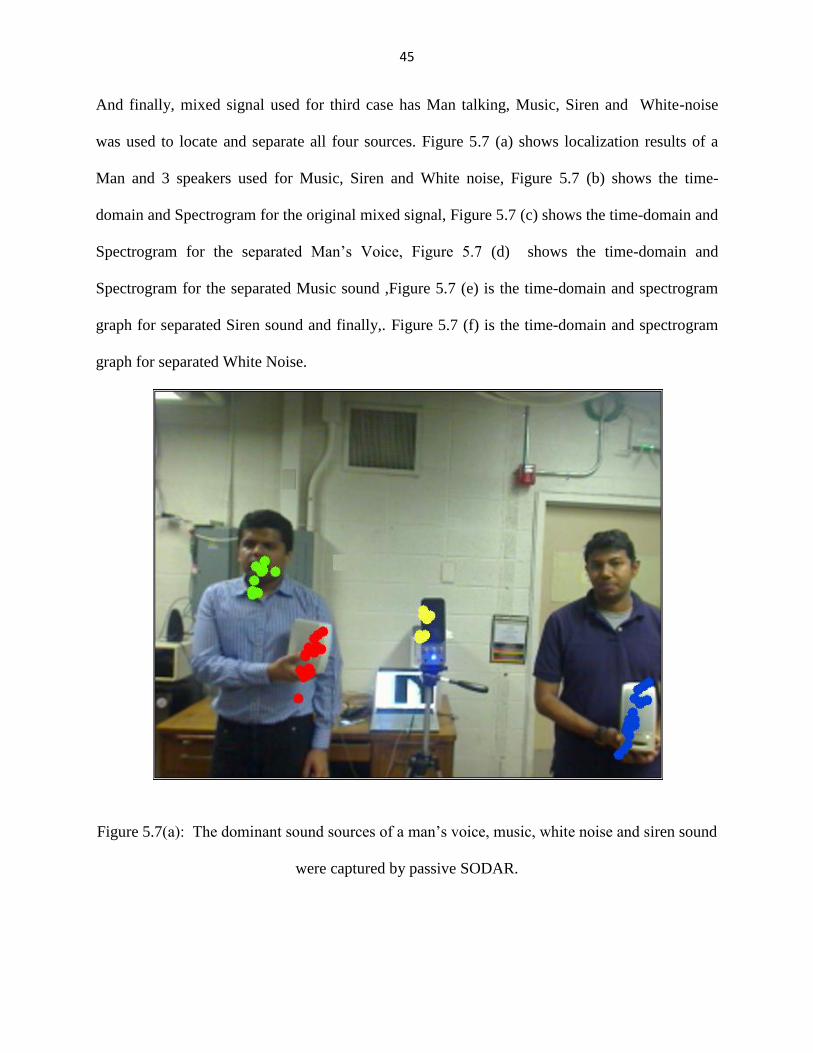
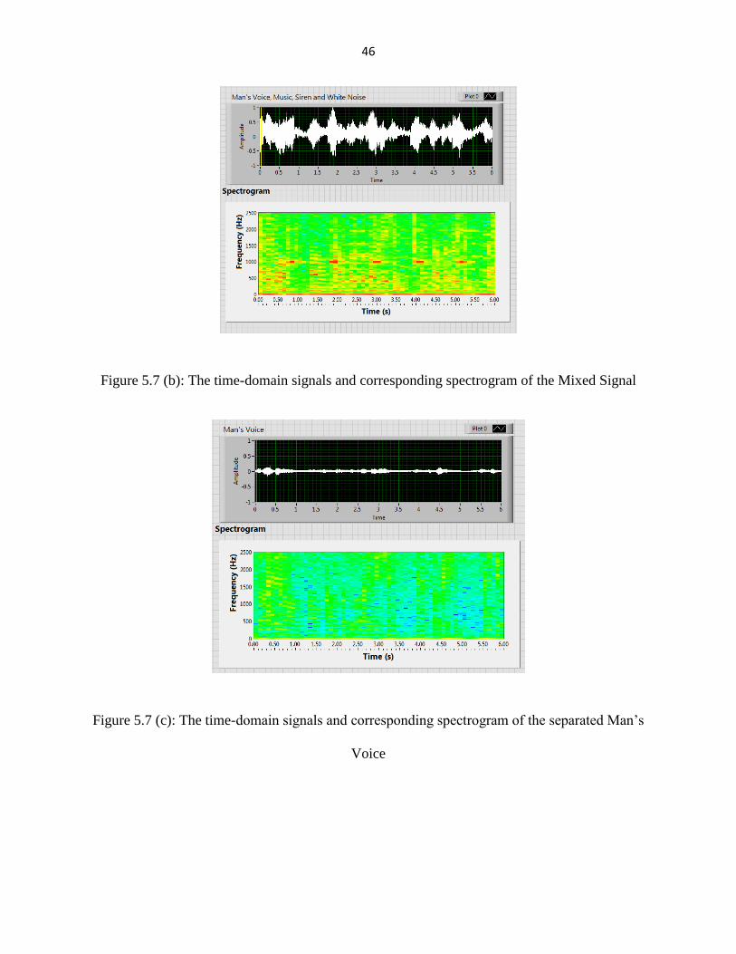
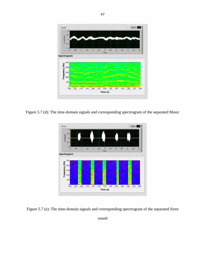
And finally, mixed signal used for third case has Man talking, Music, Siren and White-noise
was used to locate and separate all four sources. Figure 5.7 (a) shows localization results of a
Man and 3 speakers used for Music, Siren and White noise, Figure 5.7 (b) shows the time-
domain and Spectrogram for the original mixed signal, Figure 5.7 (c) shows the time-domain and
Spectrogram for the separated Man’s Voice, Figure 5.7 (d) shows the time-domain and
Spectrogram for the separated Music sound ,Figure 5.7 (e) is the time-domain and spectrogram
graph for separated Siren sound and finally,. Figure 5.7 (f) is the time-domain and spectrogram
graph for separated White Noise.
Figure 5.7(a): The dominant sound sources of a man’s voice, music, white noise and siren sound
were captured by passive SODAR.
46
Figure 5.7 (b): The time-domain signals and corresponding spectrogram of the Mixed Signal
Figure 5.7 (c): The time-domain signals and corresponding spectrogram of the separated Man’s
Voice
47
Figure 5.7 (d): The time-domain signals and corresponding spectrogram of the separated Music
Figure 5.7 (e): The time-domain signals and corresponding spectrogram of the separated Siren
sound
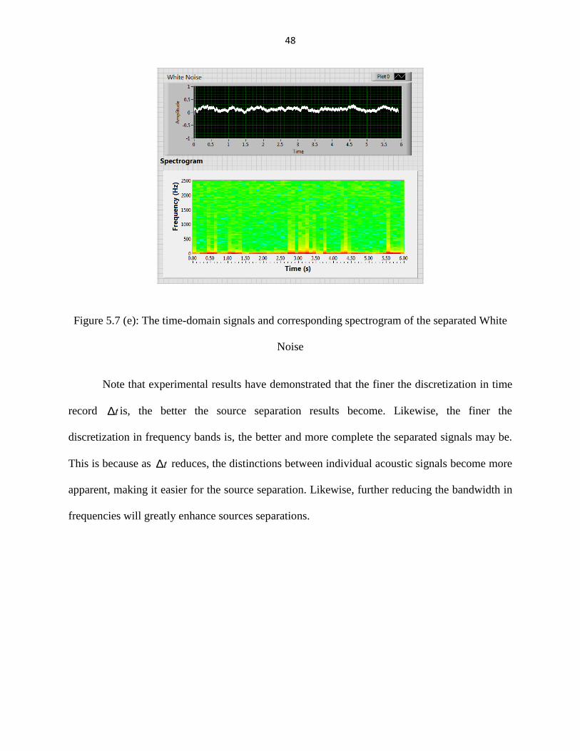
48
Figure 5.7 (e): The time-domain signals and corresponding spectrogram of the separated White
Noise
Note that experimental results have demonstrated that the finer the discretization in time
record Dt is, the better the source separation results become. Likewise, the finer the
discretization in frequency bands is, the better and more complete the separated signals may be.
This is because as Dt reduces, the distinctions between individual acoustic signals become more
apparent, making it easier for the source separation. Likewise, further reducing the bandwidth in
frequencies will greatly enhance sources separations.
49
CHAPTER 6
CONCLUSIONS
In this thesis, we have presented an innovative idea of Source Localization by using
newly developed Auto-Correlation function. Sound separation using a Signal processing
technique is also studied.
Some source localization methods were discussed in the early chapters and also various
parameters involved in Time difference of arrival calculation using Cross-correlation and Auto-
correlation were discussed in some detail.
We first discussed about Cross-correlation method to find TDOA and then new
formulations using Auto-correlation functions were discussed. This included estimation of
TDOA, counting the number of multi-paths and arrival time in both cross and auto-correlation
functions.
Another innovative technology was discussed to extract the target signal from directly
measured mixed signals. A new technology known as Short time source localization and
separation (SLAS) was presented in this thesis. Various parameters like Fourier transform, Short
time Fourier transform, Window functions were discussed.
Finally we validated all the newly developed technology by comparing the source
localization results between Cross and Auto-correlation functions. Results demonstrated that the
error in source localization was reduced by 50 % in case of Auto-correlation functions.
We then used SLAS technique to separate the target signals from directly measured
acoustic signals. The tests were carried out in AVNC lab, Wayne state university. Three cases
50
were studied and the time-domain graphs and Spectrogram of both, mixed signals and separated
signals were presented.
The passive SODAR [30] and short-time SLAS algorithms were used to perform
completely blind sources localization and separation in a highly non-ideal environment. The
accuracy in blind source separations can be further improved by decreasing the time segment Dt
and using a much finer user-defined frequency band than the standard octave bands. The
proposed method could potentially have a significant impact on a number of sectors, including
the Homeland Security, defense industries, and manufacturing industries to identify products
noise problems as well as improving the product quality issues.
51
CHAPTER 7
FUTURE WORK
The research performed in this thesis on source localization and separation has produced
satisfactory results. However, there is much room for further improvements both theoretically
and experimentally.
The auto-correlation functions have to be tested with source kept far away from the
micro-phones (greater than 3m). This requires some mathematical formulations to be developed
in order to achieve accurate results.
The SLAS technique has been tested to work well in case of speech signals but no
concrete tests have been performed with the acoustic signals from the automobiles or the
machines operating in the industry. Some testing needs to be performed at that end and
parametric studies need to be taken care in case of mechanical signals.
Lastly, some of the signal processing techniques needs to be used in order to get more
refined separated signals.
52
REFERENCES
[1] Bell, A. and Sejnowski, T. (1995). An information-maximization approach to blind
separation and blind deconvolution, Neural Computation, 7:1129– 1159.
[2] C. Jutten and J.Herault, “Blind separation of sources, part 1: An adaptive algorithm based
on neuromimetic architecture,” Signal Process. 24, 1-10 (1991).
[3] J.F. Cardoso and B.H. Laheld, “Equivariant adaptive source separation,” IEEE
Trans.Signal Process. 44. 3017-3030 (1996).
[4] A. Belouchrani, K.AbedMeraim, J.F.Cardoso and E.Moulined, “A blind source separation
technique using second-order statistics,” IEEE Trans. Signal Process. 45, 434-444 (1997).
[5] R.M. Parry, “Separation and analysis of multichannel signals, “Ph.D.thesis, Georgia
Institute of Tech., Atlanta, GA, 2007, Chap.3, pp.18-52.
[6] Tobias, A. “Acoustic-Emission source location in two dimensions by an array of three
sensors,” Non-Destructive Testing, Vol. 9, 9 – 12 (1976).
[7] Spiesberger, J. L. and Fristrup, K. M., “Passive localization of calling animals and
sensing of their acoustic environment using acoustic tomography,” American Naturalist,
Vol.135, 107 – 153 (1990).
[8] Ziola, S. M. and Gorman, M. R. “Source location in thin plates using cross-correlation”,
Journal of the Acoustical Society of America, Vol. 90, 2551 – 2556 (1991).
[9] Thode, A. M., Kuperman, W. A., D’Spain, G. L., and Hodgkiss, W. S., “Localization
using Bartlett matched-field processor sidelobes,” Journal of the Acoustical Society of
America, Vol. 107, 278 – 286 (2000).
53
[10] D’Spain, G. L., Terrill, E., Chadwell, C. D., Smith, J. A., and Lynch, S. D., “Active
control of passive acoustic fields: Passive synthetic aperture/Doppler beamforming with
data from an autonomous vehicle,” Journal of the Acoustical Society of America, Vol.
120, 3635 – 3654 (2006).
[11] Tao, H. and Krolik, J. L., “Waveguide invariant focusing for broadband beamforming in
an oceanic waveguide,” Journal of the Acoustical Society of America, Vol.123, 1338 –
1346 (2008).
[12] Fink, M., ‘‘Time reversed acoustics,’’ Physics Today, Vol. 50, 34 (1997).
[13] Yon, S., Tanter, M., and Fink, M., ‘‘Sound focusing in rooms: The time reversal
approach,’’ Journal of the Acoustical Society of America, Vol. 113, 1 – 11 (2003).
[14] Kuperman, W. A. Hodgkiss, W. S., Song, H. C., Akal, T., Ferla, C., and Jackson, D. R.,
“Phase conjugation in the ocean: Experimental demonstration of an acoustic time-
reversal mirror,” Journal of the Acoustical Society of America, Vol. 103, 25 – 40 (1998).
[15] J. P. Ianniello, "Time-delay estimation via cross-correlation in the presence of large
estimation errors," IEEE Transactions on Acoustics Speech and Signal Processing, vol.
30, pp. 998-1003, 1982.
[16] J. P. Ianniello, "Time-delay estimation via cross-correlation in the presence of large
estimation errors," IEEE Transactions on Acoustics Speech and Signal Processing, vol.
30, pp. 998-1003, 1982.
[17] W. Lindemann, "Extension of a binaural cross-correlation model by contralateral
inhibition. I. Simulation of lateralization for stationary signals," Journal of the Acoustical
Society of America, vol. 80, pp. 1608-22, Dec 1986.
54
[18] Y. Barshalom, F. Palmieri, A. Kumar, and H. M. Shertukde, "Analysis of wide-band
cross-correlation for time-delay estimation," IEEE Transactions on Signal Processing,
vol. 41, pp. 385-387, Jan 1993.
[19] A. H. Quazi, "An overview on the time-delay estimate in active and passive systems for
target localization," IEEE Transactions on Acoustics Speech and Signal Processing, vol.
29, pp. 527-533, 1981.
[20] B. M. Bell and T. E. Ewart, ‘‘Separating multipaths by global optimization of a
multidimensional matched filter,’’ IEEE Trans. Acoust. Speech Signal Process. 34,
1029–1037, ~1986!.
[21] R. J. Vaccaro and T. Manickam, ‘‘Time-delay estimation for deterministic transient
signals in a multipath environment,’’ IEEE International Conferenceon Acoustics,
Speech and Signal Processing, ICASSP-92 ~IEEE, New York, 1992!, Vol. 2, pp. 549–
552.
[22] T. G. Manickam, R. J. Vaccaro, and D. W. Tufts, ‘‘A least-squares algorithm for
multipath time-delay estimation,’’ IEEE Trans. Signal Process.42, 3229–3233 ~1994!.
[23] A. B. Baggeroer, ‘‘Matched field processing: source localization in waveguides,’’ in
Conference Record of the Twenty-Sixth Asilomar Conferenceon Signals, Systems and
Computers, Pacific Grove, CA, edited by A. Singh ~IEEE, New York, 1992!, Vol. 2, pp.
1122–1126.
[24] R. J. Vaccaro, C. S. Ramalingam, and D. W. Tufts, ‘‘Least-squares time delay estimation
for transient signals in a multipath environment,’’ J. Acoust. Soc. Am. 92, 210–218
~1992!.
55
[25] M. Raffy and C. Gregoire, "Semi-empirical models and scaling: a least square method for
remote sensing experiments," International Journal of Remote Sensing, vol. 19, pp. 2527-
2541, Sep 10 1998.
[26] M. McKeown, D. Torpey, and G. W., “Non-invasive monitoring of functionally distinct
muscle activations during swallowing,” Clinical Neurophysiology, vol. 113, no. 3, pp.
354–66, 2002.
[27] J. Anemuller, “Adaptive separation of acoustic sources for anechoic conditions: A
constrained frequency domain approach,” Speech Communication, vol. 39,no. 1-2, pp.
79–95, 2003.
[28] S. Rickard, R. Balan, and J. Rosca, “Real-time time-frequency based blind source
separation,” in 3rd International Conference on IndependentComponent Analysis and
Blind Source Separation, San Diego, CA, December 9-12 2001.
[29] R. Crochiere, “A weighted overlap-add method of short-time fourier analysis/ synthesis,”
IEEE Transactions on acoustics, speech, and signal processing vol. ASSP-28, no. 1, pp.
99–102, 1980.
[30] S. F. Wu and N. Zhu, “Passive sonic detection and ranging for locating sound sources,”
(to appear in Journal of the Acoustical Society of America, 2013).
[31] John L. Spiesberger, “Identifying cross-correlation peaks due to multipaths with
application to optimal passive localization of transient signals and tomographic mapping
of the environment,” January 1996.
[32] John L. Spiesberger, “Linking auto- and cross-correlation functions with correlation
equations: Application to estimating the relative travel times and amplitude of multipath,”
April 1998.
56
[33] Zhu, Na, "Locating and extracting acoustic and neural signals" . Wayne State
University Dissertations. January 2011.
[34] S.F. Wu, Raghavendra Kulkarni, Srikanth Duraiswamy, “An autonomous surveillance
system for blind sources localization and separation ( Submitted April 2013).
[35] S.F. Wu and N.Zhu, “Locating arbitrarily time-dependent sound sources in three
dimensional space in real time”, May 2010.
[36] S.F. Wu and N.Zhu, “Sound source localization in three dimensional space in real
time with redundancy checks”, March 2012.
57
ABSTRACT
DEVELOPING A SYSTEM FOR BLIND ACOUSTIC SOURCE LOCALIZATION AND
SEPARATION
by
RAGHAVENDRA KULKARNI
August 2013
Advisor: Dr. Sean F. Wu
Major: Mechanical Engineering
Degree: Master of Science
This thesis presents innovate methodologies for locating, extracting, and separating
multiple incoherent sound sources in three-dimensional (3D) space; and applications of the time
reversal (TR) algorithm to pinpoint the hyper active neural activities inside the brain auditory
structure that are correlated to the tinnitus pathology. Specifically, an acoustic modeling based
method is developed for locating arbitrary and incoherent sound sources in 3D space in real time
by using a minimal number of microphones, and the Point Source Separation (PSS) method is
developed for extracting target signals from directly measured mixed signals. Combining these
two approaches leads to a novel technology known as Blind Sources Localization and Separation
(BSLS) that enables one to locate multiple incoherent sound signals in 3D space and separate
original individual sources simultaneously, based on the directly measured mixed signals. These
technologies have been validated through numerical simulations and experiments conducted in
various non-ideal environments where there are non-negligible, unspecified sound reflections
and reverberation as well as interferences from random background noise. Another innovation
presented in this thesis is concerned with applications of the TR algorithm to pinpoint the exact
58
locations of hyper-active neurons in the brain auditory structure that are directly correlated to the
tinnitus perception. Benchmark tests conducted on normal rats have confirmed the localization
results provided by the TR algorithm. Results demonstrate that the spatial resolution of this
source localization can be as high as the micrometer level. This high precision localization may
lead to a paradigm shift in tinnitus diagnosis, which may in turn produce a more cost-effective
treatment for tinnitus than any of the existing ones.
59
AUTOBIOGRAPHICAL STATEMENT
RAGHAVENDRA KULKARNI
EDUCATION:
2013, MS (Mechanical Engineering): Wayne State University, Detroit.
2010, BE (Mechanical Engineering): Gogte Institute of Technology,
Belgaum, India.
AWARD:
Recipient of Wayne State University Graduate Teaching Assistant scholarship from
Jan’12-May’13