Acoustic emission source localization and velocity

determination of the fundamental mode A0 using wavelet

analysis and a Newton-based optimization technique

F. Ciampa, M.Meo

Material Research Centre, Department of Mechanical Engineering,

University of Bath, Bath, UK

Abstract

This paper investigates the development of an in-situ impact detection

monitoring system able to identify in real-time the acoustic emission location. The

proposed algorithm is based on the differences of stress waves measured by surface

bonded piezoelectric transducers. A joint time frequency analysis based on the

magnitude of the Continuous Wavelet Transform was used to determine the time of

arrivals of the wave packets. A combination of unconstrained optimization technique

associated to a local Newton’s iterative method was employed to solve a set of non

linear equations in order to assess the impact location coordinates and the wave speed.

With the proposed approach, the drawbacks of a triangulation method in terms to

estimate a priori the group velocity and the need to find the best time-frequency

technique for the time of arrival determination were overcome. Moreover, this

algorithm proved to be very robust since it was able to converge from almost any guess

point and required little computational time. A comparison between the theoretical and

experimental results carried out with piezoelectric film (PVDF) and acoustic emission

transducers showed that the impact source location and the wave velocity were

predicted with reasonable accuracy. In particular, the maximum error in estimation of

the impact location was less than 2% and about 1% for the flexural waves velocity.

Keywords: Impact location identification, Continuous Wavelet Transform, PVDF,

flexural waves.

1 Introduction and statement of the problem

A real-time knowledge of the impact location source is fundamental in both

Non-Destructive Evaluation (NDE) techniques as well as Structural Health Monitoring

(SHM) systems. The ability to locate the impact response can be achieved through

passive technique, wherein the signals emitted by internal or external sources are

measured by ultrasonic transducers directly on the specimen surface or embedded into

the structure (Balageas et al., 2006).

Most of these techniques deal with the detection of Lamb waves caused by low

velocity impacts. According to Viktorov (1967) theory, Lamb waves are stress waves

that propagate within thin solid plates with free boundaries. Depending on the product

of frequency times thickness, an infinite number of modes for both symmetric and

antisymmetric displacements are available. Symmetric modes (Sn) are related to the

extensional modes as displacements occur in the direction of wave propagation, whilst

antisymmetric modes (An) are known as flexural modes as the displacements pattern is

transverse to the plane of the plate. These Lamb modes differ in their phase and group

velocities as well as in the strain and stress field.

Estimating the location of an AE source is an inverse problem based on the

detection of the time at which the stressed wave reaches a number of sensors. Several

studies presents in literature were focused on the in situ investigations of Lamb waves

using piezoelectric transducers attached to plate-like structures (El youbi et al., 2004;

Giurgiutiu, 2002). An alternative to these conventional transducers was the employment

of polyvinyldilene fluoride (PVDF) film sensors for AE applications (Hamstad M A,

1995; Brown et al., 1996; Gaul and Hurlebaus, 1999; Monkhouse et al., 2000). These

smart materials bonded on the surface of the structures own the characteristic of better

interrogate large areas with a low cost availability, easily handle and broad-band

acoustic performance.

Usually, most of the methods for impact location use the triangulation technique

(also known as Tobias algorithm), wherein the impact point is identified as the

intersection of three circles, whose centres are the sensors location (Tobias, 1976). This

approach is strongly limited by the assumption that wave velocity must be known and

remains the same in all directions, but this is not true especially in anisotropic and

inhomogeneous materials. Moreover, the flexural wave velocity is not constant, but it is

function of the signal frequency that depends on the impact speed of the object hitting

the structure.

Furthermore, due to the dispersive nature of the flexural modes or to the

uncertainty of the noise level of the signal measured, a suitable choice of the time–

frequency analysis for the identification of the time of arrival (TOA) is necessary. In

these terms, Ziola and Gorman (1991) employed a cross-correlation technique for

determining the time of propagation, whilst Kosel et al. (2003) used a combination of

cross-correlation function with an appropriate bandpass-filter. In both approaches the

maximum of the cross-correlation coefficient of two signals indicates the delay time

between them. However, these methods present such limits especially when the sensors

are placed close to the edges. In fact, multiple reflections from the boundaries generate

ambiguous peaks in cross-correlation coefficients causing poor localisation results.

Seydel and Chang (2001) proposed an approach based on a double peak method

wherein the arrival time was chosen by selecting the minimum before the maximum for

each signal. Nevertheless, the dependence of the wave velocity on frequency and the

ambiguity of the noise level make this method inappropriate for the purpose of correct

determination of the impact source. Therefore the use of the Continuous Wavelet

Transform (CWT) that provides high resolution for a wide range of frequencies was

found to guarantee more accuracy in the time-frequency analysis of acoustic waves (e.g.

Meo et al., 2005; Jeong and Jung, 2000).

Real-time impact algorithms must exhibit the best tradeoffs in terms of efficiency

and accuracy and must require very little computational time (CPU cost) for different

use in a SHM system. Kundu et al. (2009) developed an optimization algorithm for the

determination of point of impact on aluminium and composite structures, based on

minimizing an error function that used the difference of TOA of AE signals. Gaul et al.

(2001) applied a Gauss-Newton method to non linear least square optimization to

analyze “synthetic” AE signals. Conversely, an alternative approach to model-based

methods for the identification of the impact location was the artificial neural network

approach (Sung et al., 2000). Despite this method is suitable for complex structure, it

cannot provide an optimum solution.

The research study conducted in this paper was aimed to overcome the limits of

a triangulation method for a real-time localization of the impact source and to exhibit

the best approach for the time of arrival determination. In fact, the present work reports

the creation of an algorithm for in-situ impact detection (AE) and wave velocity

identification in isotropic structures, using a network of piezoelectric transducers. To

assess the impact location and the wave velocity, the basic idea was to combine a

globally convergent strategy, based on an unconstrained optimization associated to a

local Newton-Raphson iterative method. In addition, the information contained in the

time-frequency graph of the magnitude of the Continuous Wavelet Transform was used

to determine the time of propagation of the stress waves. To validate the method, two

different experiments with piezoelectric-film (PVDF) and Acoustic Emission sensors

were carried out. Figure 1 illustrates the architecture of the impact location and wave

velocity determination system.

The layout of the paper is as follow: in Section 2 the algorithm for the source

location and wave velocity evaluation algorithm is presented. Section 3 outlines the

main characteristics of the Continuous Wavelet Transform in terms of multi-resolution

analysis and energy density of the signal for the time of arrival identification. In Section

4 the local Newton’s iterative method associated to an unconstrained optimization for

solving systems of non-linear equations is described. Section 5 reports the experimental

set-up and the analysis results. Then, the final conclusions of the method adopted are

discussed.

Figure 1 Architecture of impacts source location and wave velocity identification system

2 Impact location and group wave velocity algorithm

The algorithm for the impact source location and wave velocity determination is based

on the differences of acoustic emission (AE) signals measured by four piezoelectric

transducers attached on the surface of an aluminium structure. As the medium of

interest is isotropic and homogeneous, from classical theory of thin elastic plate (Reddy,

1999), the extensional wave group velocity 21

E

cl and the flexural wave

velocity

41

2

2

2

112

Ehc f are related by only density , thickness h, angular

frequency , Young modulus E and Poisson ratio . Hence, in this algorithm, the

group velocity can be considered independent of propagation direction.

The origin of the Cartesian reference frame was arranged at the left bottom

corner of the plate. The impact source point I is at unknown coordinates II yx , in the

plane of the plate and the sensors are located at distance id 4,,1i from the source

(Fig. 2). Furthermore, the dimensions of the plate are L, length and W, width.

Figure 2 Impact location and wave velocity identification procedure

The resulting system of equation for the source location problem and wave

speed identification is given as follow:

22

IiIii yyxxd (2.1)

g

ii

V

dt (2.2)

where gV is the velocity of propagation of the stressed wave, it is the time of detection

of the AE signals and ii yx , are the coordinates of the i-th sensor. Combining

equations (2.1) and (2.2) we obtain:

0222 giIiIi Vtyyxx (2.3)

which is the equation of circumference with radius 22

gi Vtr . Equation (2.3)

can be expanded into the following set of equations, with the unknown it , Ix , Iy and

gV :

0

0

0

0

2

4

2

4

2

4

2

3

2

3

2

3

2

2

2

2

2

2

2

1

2

1

2

1

gII

gII

gII

gII

Vtyyxx

Vtyyxx

Vtyyxx

Vtyyxx

(2.4)

This is a system of four equations with seven unknown. If 1t is the travel time

required to reach the sensor 1 (master sensor) and jt1 4,3,2j are the time

difference between the sensor 1 and the other sensors, we can write:

1414

1313

1212

ttt

ttt

ttt

(2.5)

and system (2.4) becomes:

0

0

0

0

2

141

2

4

2

4

2

131

2

3

2

3

2

121

2

2

2

2

2

1

2

1

2

1

gII

gII

gII

gII

Vttyyxx

Vttyyxx

Vttyyxx

Vtyyxx

(2.6)

Location and wave velocity must be calculated by solving this set of non linear

equations with the unknown gII Vtyx ,,, 1x . The three time differences jt1 must be

determined through an appropriate time-frequency analysis.

Next Section outlines the characteristics of the Continuous Wavelet Transform

for the time of wave propagation identification, whilst Section 3 describes the algorithm

aimed to solve the set of non linear equations (2.6) for the assessment of the impact

location coordinates and the speed of Lamb wave 0A .

3 The Continuous Wavelet Transform

Due the dependence of the wave velocity on frequency and the ambiguity of the noise

level, a good impact detection method necessitates of a suitable choice of the time–

frequency analysis for the time arrival identification.

Wavelet transformation method provides a good compromise between location

and frequency resolution and it is able to analyze low and high frequencies at the same

time, even respecting the uncertainty principle (also known as Heisenberg inequality).

Let 21 LL be the analysing wavelet called also the mother wavelet, where

is the domain of real numbers and the space 2L is the set of all square-integrable

functions defined on . The mother wavelet must satisfy the admissibility condition

defined as:

d

2ˆ

(3.1)

where ̂ is the Fourier transform of . Eq. (3.1) is the necessary condition for ensuring

the existence of the inverse wavelet transform. The Continuous Wavelet Transform

(CWT) is a linear transform that decomposes an arbitrary signal )(tf through basis

functions that are simply dilatations and translations of a parent wavelet )(t , by the

continuous convolution of the signal and the scaled or shifted wavelet (Mallat, 1998):

dta

bttf

attfbaWT ba

1),( , (3.2)

where t denotes the complex conjugate of the mother wavelet )(t , a is the

dilatation or scale parameter defining the support width of the wavelet and b the

translation parameter localising the wavelet in the time domain. The factor a1 is used

to ensure that all wavelets at all scales have the same area and contain the same energy.

The time-frequency resolution of the wavelet transform can be expressed as

function of the scale parameter a through the following relationships:

m

m

a

tat (3.3)

where t and are the duration and bandwidth of the wavelet function,

respectively, and Zm with Z the set of positive integers.

According to the uncertainty principle (Le and Argoul, 2004), time-frequency

localization domain for any time frequency point is a rectangle of width tam and

height ma with a constant area of ft . Consequently, time resolution of the CWT

increases as frequency decreases and frequency resolution increases as time decreases.

For these reasons, differently from the Short Time Fourier Transform wherein

resolution is constant, the CWT is called multi-resolution analysis.

3.1 Morlet wavelet

Several studies present in literature deal with the use of the wavelet transform

applied to acoustic emission (Hamstad et al., 2002). Gaul and Hurlebaus (1999) and

Jeong and Jung (2000) applied the Gabor wavelet to identify the coordinates of an

impact load on aluminium plate and Meo et al. (2005) used the Morlet wavelet to detect

a source location of an acoustic emission on CFRP composite panel. In this study

complex Morlet wavelet was employed as, in contrast with real wavelets, is able to

separate amplitude and phase, enabling the measurement of instantaneous frequencies

and their temporal evolution (Mallat S., 1998). Furthermore, it was experienced (Meo et

al., 2005) that Morlet wavelet enables the measurement of the localization frequency for

signals with faster and slower oscillations, providing a flexible window that narrows at

high frequencies and widens when observing low-frequency phenomena. The complex

Morlet wavelet is expressed by the following equation:

tjteF

eeF

t cc

F

t

b

F

t

tj

b

bbc

sincos

1122

(3.4)

Morlet wavelet seems like an impulsive waveform with a central frequency

2ccf when its shape control parameter bF (wavelet bandwidth) can be set to be

a small value. Conversely, when bF increases, the wavelet waveform tends to be a

harmonic waveform (Fig. 3). However, for practical purposes, because of the fast decay

of its envelope towards zero, Morlet wavelet is considered admissible for 5c .

Furthermore, maximising equation (3.4) in the frequency domain, we obtain a unique

relation between the scale parameter a and frequency of interest f:

a

ff c (3.5)

22

ˆ cb ffaFeaf

(3.6)

where af̂ is the Fourier transform of t .

Figure 3 (a) (b) (c) (d) Morlet wavelet with different values of Fb (1.5 blue colour, 0.1 red colour). In

figures (a) and (b) are represented the real and imaginary part of Morlet wavelet, whilst figures (c) and (d)

depict the modulus and the phase angle.

3.2 Time of arrival identification using the CWT

CWT coefficients are useful for the identification of non stationary signals like transient

phenomena hidden in vibration signals or impacts (Kim and Melheim, 2004).

In particular, the real part of the CWT is well suited for the determination of

dominant scales, whilst the squared modulus of the CWT called also scalogram

indicates the energy density of the signal at each scale at any time (Mallat S., 1998).

Hence, the scalogram is able to reveal the highest local energy content of the waveform

measured. The squared modulus can be express as:

),(),(),(2

baWTbaWTbaWT (3.7)

Furthermore, the maximum value of the coefficients of the scalogram with a

high concentration of energy is achieved at the instantaneous frequency, corresponding

to the dominant frequency in the signal analysed at each instant in time. These

coefficients taken at the instantaneous frequency in a time-frequency domain determine

the ridges (Mallat S., 1998; Haase and Widjajakusuma, 2003). Therefore, the frequency

of interest is chosen as the dominant frequency in the signal analysed by each sensor at

each instant in time, i.e. the frequency corresponding at the maximum value of the

Continuous Wavelet Transform squared modulus coefficients (ridges). Each frequency

of interest is related to the scale parameter by the following relationship:

aT

ffreq c (3.8)

where freq is the frequency of interest, cf is the central frequency of the wavelet used

and T is the sampling period. The projection on the time domain of the ridge

corresponds to the time of arrival (TOA) of the stress waves (Fig. 4). Once the TOA is

known, we can calculate the time differences jt1 (eq. 2.5) with respect to the master

sensor. Hence, based on the algorithm discussed in the next Section, the coordinates of

the impact source location and wave group velocity can be determined.

Figure 4 3-D plot of the scalogram of the CWT in which the ridge is took at the instantaneous frequency

of 310 kHz

4 Newton’s method for solving systems of non-linear equations

The strategy adopted in this paper to solve the set of equations (2.6) and to make

the algorithm robust and convergent from almost any guess point is to combine a

Newton’s method with a Line Search algorithm.

Newton-Raphson or Newton’s method is a very efficient iterative algorithm for

finding the roots of non linear system of equations, since it locally converges from

around an initial guess point 0x sufficiently close to the root (Dennis, 1996).

Let assume nn

iF : , where n denotes n-dimensional Euclidean space, to

be a twice Lipschitz continuously differentiable function. The set of non linear equations

(2.6) can be expressed as:

0xF (4.1)

where F is the vector of the functions iF ( 4,,1i ) and x is the vector of

unknown jx ( 4,,1j ). Equation (4.1) has a zero at nx such that 0xF .

Newton’s method converges quadratically to

x (i.e. the order of convergence is

approximately two) by computing the Jacobian linearization of the function F around a

guess point 0x , and then using this linearization to move closer to the desired zero. The

Newton iterate 1n

x from a current point n

x is given by:

nnnnnnxFxJxxxx

11 (4.2)

where xFxJx 1

is the Newton step and xJ is the Jacobian matrix,

which contains first derivatives of the objective function xF with respect to the four

unknowns of the problem:

gII

gII

gII

gII

V

F

t

F

y

F

x

F

V

F

t

F

y

F

x

F

V

F

t

F

y

F

x

F

V

F

t

F

y

F

x

F

xxxx

xxxx

xxxx

xxxx

x

xFxJ

4

1

444

3

1

333

2

1

222

1

1

111

(4.3)

Newton’s method can be modified and enhanced in various ways for solving

systems of non linear equations, but in particular conditions, when the starting point is

not near the root, it may not converge (Nocedal, 1999). The reasons for this failure are

that the direction of the current iterate n

x may differ to be a direction of descent for F ,

and, even if a search direction is a direction of decrease of F , the length of the Newton

step x may be too long. Hence, a globally convergent algorithm associated to a

Newton’s method can be designed to find the solution of a system of non linear

equations from almost any guess point 0x . The approach adopted in this paper was to

combine the Newton’s method applied to the system (2.6) with the unconstrained

problem of minimizing the objective function F:

n

x n:min F (4.4)

In unconstrained optimization, the most widely used function to be minimized

(also known as merit function) is a scalar-valued function of F , i.e. the squared norm of

F :

xFxFxFx 2

1

2

1 2f (4.5)

where the factor 2

1 is introduced for convenience. Obviously any root of f fulfils

the identity 0xf . Among the class of powerful algorithms for unconstrained

optimization, in this paper we will focus on the Line-Search methods because of its

simplicity, and because they do not depend on how the Jacobian is obtained.

Furthermore, if the initial Newton step is proved to be unsatisfactory, the polynomial

backtracking method will be considered.

4.1 Line Search methods with step selection by backtracking

In Line Search method the algorithm chooses a direction nx and searches along this

direction from the current iterate to a new iterate 1n

x that guarantees a lower value of

xf . The iteration is expressed by the following formula:

101 nnnn xxx (4.6)

where is called step length. Whether the initial iterate 0x is close to the solution, the

common strategy is to use a full Newton step nx by setting 1 . Otherwise, we move

downhill along the Newton direction trying a sufficiently small value of until 1n

x

satisfies the following criterion (known as Armijo condition):

nTnnnnnn fff xxxxx (4.7)

A good value of the parameter is 410 . The descent direction of the Newton

step from the current point n

x to a new point 1n

x is verified by the fact that the

directional derivative of f at n

x in the direction nx is negative:

0

2

1

1

nnnnnn

nnnnnf

xFxFxFxJxJxF

xxFxFxx (4.8)

Moreover, the strategy for reducing guarantees that the Newton step may not

be too large. The procedure can be performed through a backtracking Line-Search

method (Dennis, 1996). It consists in finding the value of which minimizes the model

of the following polynomial function:

nnnn fg xx (4.9)

Hence, given any descent direction nx , equation (4.9) satisfies (4.7) and (4.8) such

that:

nTnn fg xx (4.10)

Initially, the model of g is given and assumed linear:

nTn

n

fg

fg

xx

x

0

0 (4.11)

Setting 10 , if the model satisfies the following condition:

001 ggg (4.12)

we terminate the search. Otherwise, g is expressed through a quadratic

approximation by interpolating the three information available, 0g , 1g and 0g :

00001 2 ggggggq (4.13)

The new trial value 1 is defined as the minimiser of qg :

0012

0 2

01

ggg

g

(4.14)

If 1 is too small the quadratic model is poorly accurate and we set a limit value of ,

1.0min . Conversely, a cubic model of cg is more acceptable since it provides

more accuracy especially in situations where f has a negative curvature:

0023 ggbagc (4.15)

From eq. (4.15), solving with respect to the coefficients a and b, we obtain a set of two

equations using the last two previous values of ( 0g and 1g ):

22

11

3

1

3

0

2

1

2

0

01

2

1

2

0 00

001

ggg

ggg

b

a (4.16)

By differentiating eq. (4.13), the minimum point 2 is given by:

a

gabb

3

032

2

(4.17)

Therefore, if any i is either too close and smaller than 1i , i must be limited

between the values 1max 5.0 i and i 1.0min . This procedure allows obtaining

reasonable progress on each iteration, and the final will not be too small.

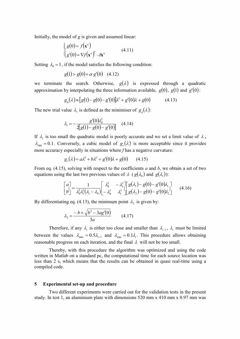
Thereby, with this procedure the algorithm was optimized and using the code

written in Matlab on a standard pc, the computational time for each source location was

less than 2 s, which means that the results can be obtained in quasi real-time using a

compiled code.

5 Experimental set-up and procedure

Two different experiments were carried out for the validation tests in the present

study. In test 1, an aluminium plate with dimensions 520 mm x 410 mm x 0.97 mm was

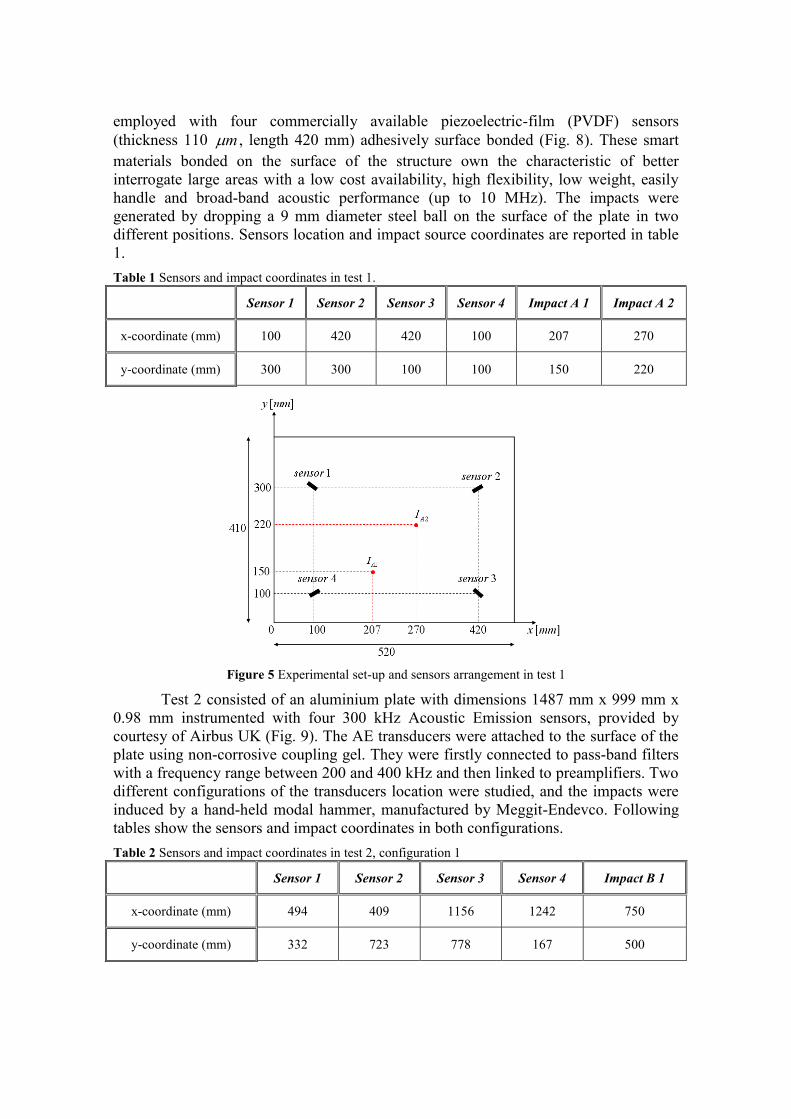
employed with four commercially available piezoelectric-film (PVDF) sensors

(thickness 110 m , length 420 mm) adhesively surface bonded (Fig. 8). These smart

materials bonded on the surface of the structure own the characteristic of better

interrogate large areas with a low cost availability, high flexibility, low weight, easily

handle and broad-band acoustic performance (up to 10 MHz). The impacts were

generated by dropping a 9 mm diameter steel ball on the surface of the plate in two

different positions. Sensors location and impact source coordinates are reported in table

1.

Table 1 Sensors and impact coordinates in test 1.

Sensor 1 Sensor 2 Sensor 3 Sensor 4 Impact A 1 Impact A 2

x-coordinate (mm) 100 420 420 100 207 270

y-coordinate (mm) 300 300 100 100 150 220

Figure 5 Experimental set-up and sensors arrangement in test 1

Test 2 consisted of an aluminium plate with dimensions 1487 mm x 999 mm x

0.98 mm instrumented with four 300 kHz Acoustic Emission sensors, provided by

courtesy of Airbus UK (Fig. 9). The AE transducers were attached to the surface of the

plate using non-corrosive coupling gel. They were firstly connected to pass-band filters

with a frequency range between 200 and 400 kHz and then linked to preamplifiers. Two

different configurations of the transducers location were studied, and the impacts were

induced by a hand-held modal hammer, manufactured by Meggit-Endevco. Following

tables show the sensors and impact coordinates in both configurations.

Table 2 Sensors and impact coordinates in test 2, configuration 1

Sensor 1 Sensor 2 Sensor 3 Sensor 4 Impact B 1

x-coordinate (mm) 494 409 1156 1242 750

y-coordinate (mm) 332 723 778 167 500

Table 3 Sensors and impact coordinates in test 2, configuration 2

Sensor 1 Sensor 2 Sensor 3 Sensor 4 Impact B2

x-coordinate (mm) 494 409 741 1156 890

y-coordinate (mm) 332 723 780 778 398

(a)

(b) Figure 6 (a) (b) Experimental set-up and sensors arrangement in test 2.

For the signal acquisition, a four channel oscilloscope (Tektronic TDS 3014)

with a sampling rate of 2 MHz was used, and it was triggered by one of the sensors

(master sensor). The time histories of the signals received by the sensors were stored on

a computer and processed using a Matlab software code implemented by the author.

6 Impact location results

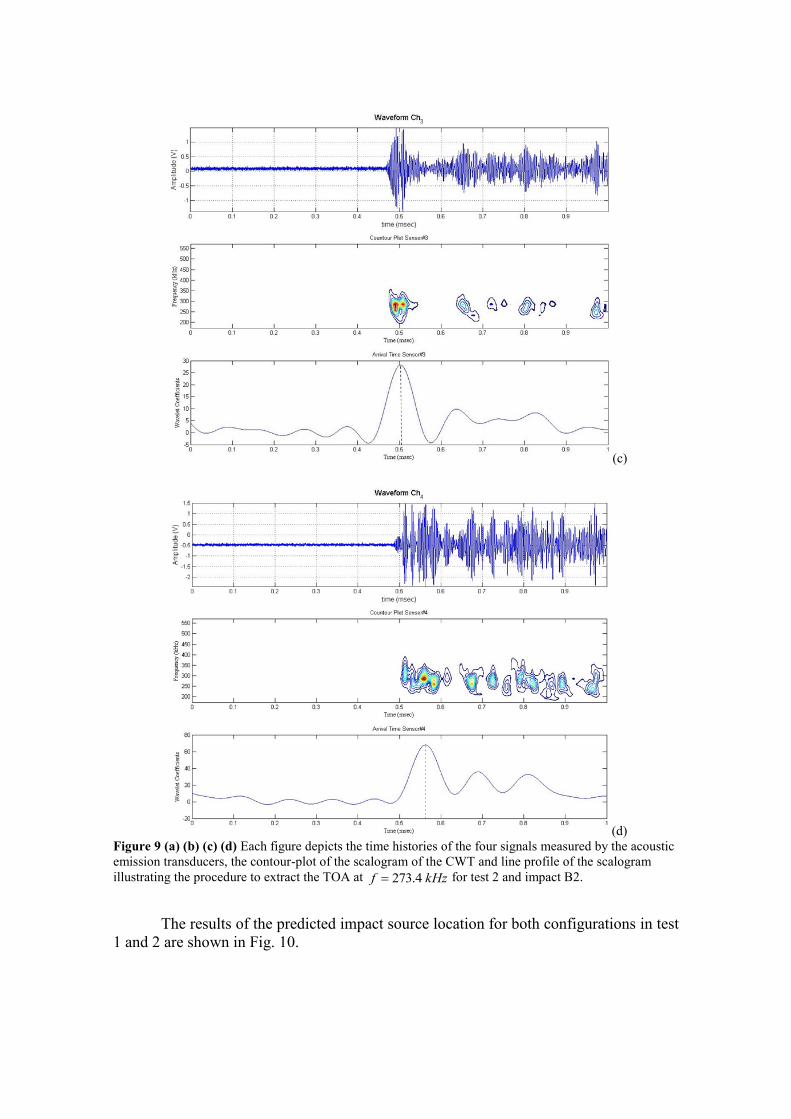
The signals were analyzed in terms of group (energy) velocity–frequency

relationship. A numerical routine was developed to find the 0A Lamb wave mode peaks

to extract the arrival time of the wave packets with largest energy contribution (ridges of

the scalogram) (Fig. 7, 8, 9). Hence, according to Section 3, the maxima coefficients of

the scalogram in both experiments were found at two different frequencies, 3452 Hz for

the tests with the PVDF (referred as A1 and A2 in the article) and 273.4 kHz with

acoustic emission transducers (referred as B1 and B2 in the article). Therefore, arrival

times of the flexural waves can be identified at these instantaneous frequencies.

Nevertheless, it was noticed that the frequencies of interest 3452 Hz for the tests with

PVDF (A1 and A2) and 273.4 kHz with acoustic emission transducers (B1 and B2)

were not the same for all four sensors. This can be seen in sub-figure (c) of Figure 7,

sub-figures (a) and (c) of Figure 8 and sub-figure (c) of Figure 9, wherein the time

representation of the wavelet coefficients does not seem to match the maximum of

contour plot of the relative scalogram. However, for those transducers for which the

scalogram maximum coefficients resulted different, the associated frequency was

approximately the same (a maximum difference of 10 Hz) with respect to the values

mentioned above. This means that the arrival time evaluation error due to this frequency

shift is negligible.

The results of the impact location and wave velocity identification are

summarized in Fig. 7 for test 1 and are reported in Fig. 8 and 9 for test 2.

(a)

(b)

(c)

(d)

Figure 7 (a) (b) (c) (d) Each sub-figure illustrates the time histories of the four signals measured by the

PVDF transducers, the contour-plot of the scalogram of the CWT and line profile of the scalogram

illustrating the procedure to extract the TOA at Hzf 3452 for test 1 and impact A1.

(a)

(b)

(c)

(d) Figure 8 (a) (b) (c) (d) Each figure illustrates the time histories of the four signals measured by the

acoustic emission transducers, the contour-plot of the scalogram of the CWT and line profile of the

scalogram illustrating the procedure to extract the TOA at kHzf 4.273 for test 2 and impact B1.

(a)

(b)

(c)

(d) Figure 9 (a) (b) (c) (d) Each figure depicts the time histories of the four signals measured by the acoustic

emission transducers, the contour-plot of the scalogram of the CWT and line profile of the scalogram

illustrating the procedure to extract the TOA at kHzf 4.273 for test 2 and impact B2.

The results of the predicted impact source location for both configurations in test

1 and 2 are shown in Fig. 10.

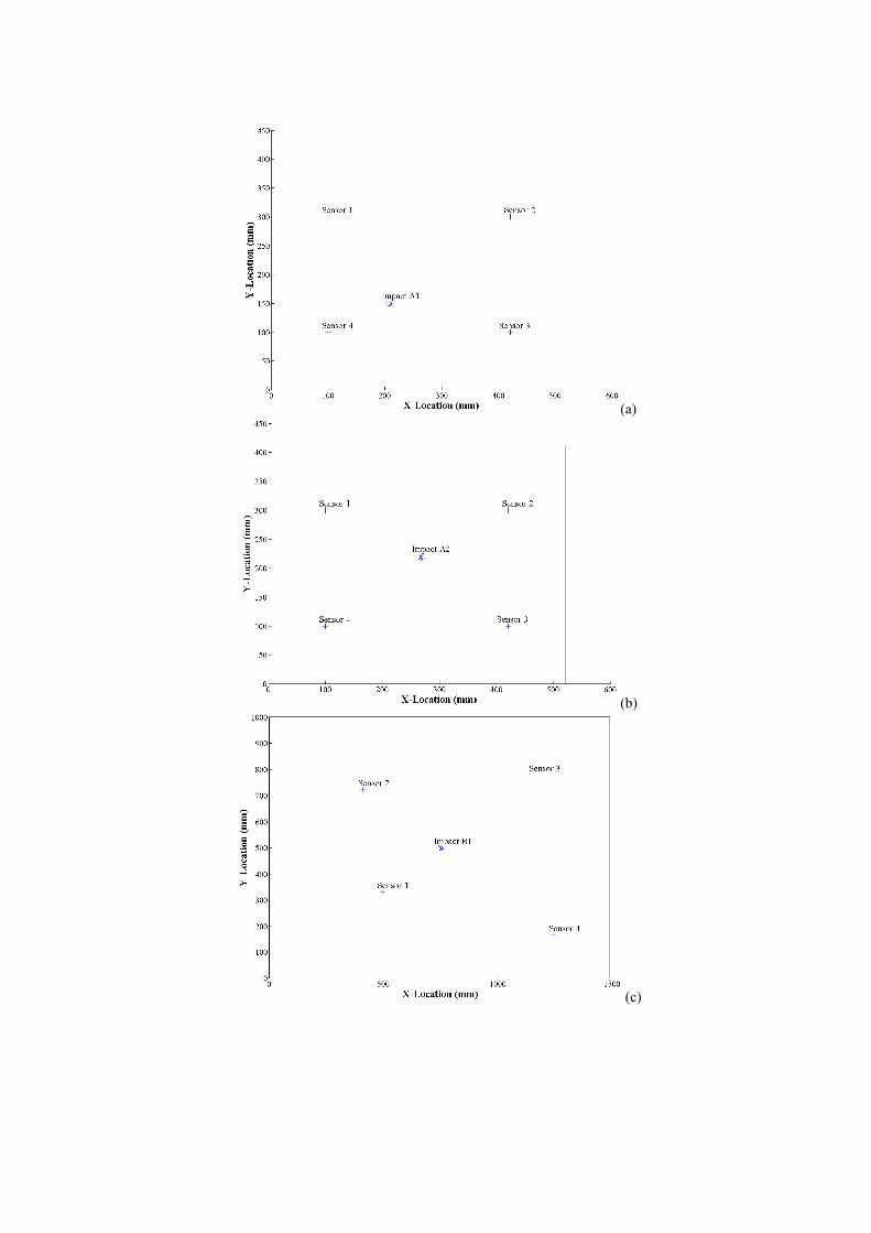
(a)

(b)

(c)

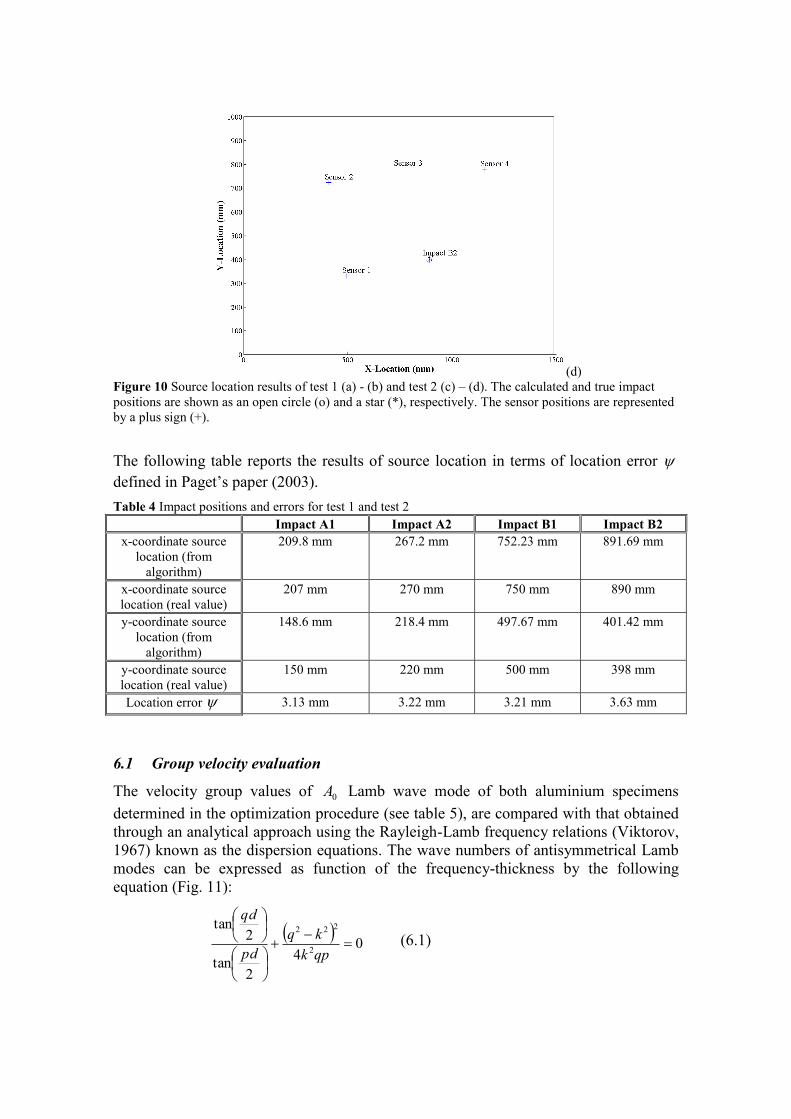
(d) Figure 10 Source location results of test 1 (a) - (b) and test 2 (c) – (d). The calculated and true impact

positions are shown as an open circle (o) and a star (*), respectively. The sensor positions are represented

by a plus sign (+).

The following table reports the results of source location in terms of location error

defined in Paget’s paper (2003).

Table 4 Impact positions and errors for test 1 and test 2 Impact A1 Impact A2 Impact B1 Impact B2

x-coordinate source

location (from

algorithm)

209.8 mm 267.2 mm 752.23 mm 891.69 mm

x-coordinate source

location (real value)

207 mm 270 mm 750 mm 890 mm

y-coordinate source

location (from

algorithm)

148.6 mm 218.4 mm 497.67 mm 401.42 mm

y-coordinate source

location (real value)

150 mm 220 mm 500 mm 398 mm

Location error 3.13 mm 3.22 mm 3.21 mm 3.63 mm

6.1 Group velocity evaluation

The velocity group values of 0A Lamb wave mode of both aluminium specimens

determined in the optimization procedure (see table 5), are compared with that obtained

through an analytical approach using the Rayleigh-Lamb frequency relations (Viktorov,

1967) known as the dispersion equations. The wave numbers of antisymmetrical Lamb

modes can be expressed as function of the frequency-thickness by the following

equation (Fig. 11):

0

4

2tan

2tan

2

222

qpk

kq

dp

dq

(6.1)

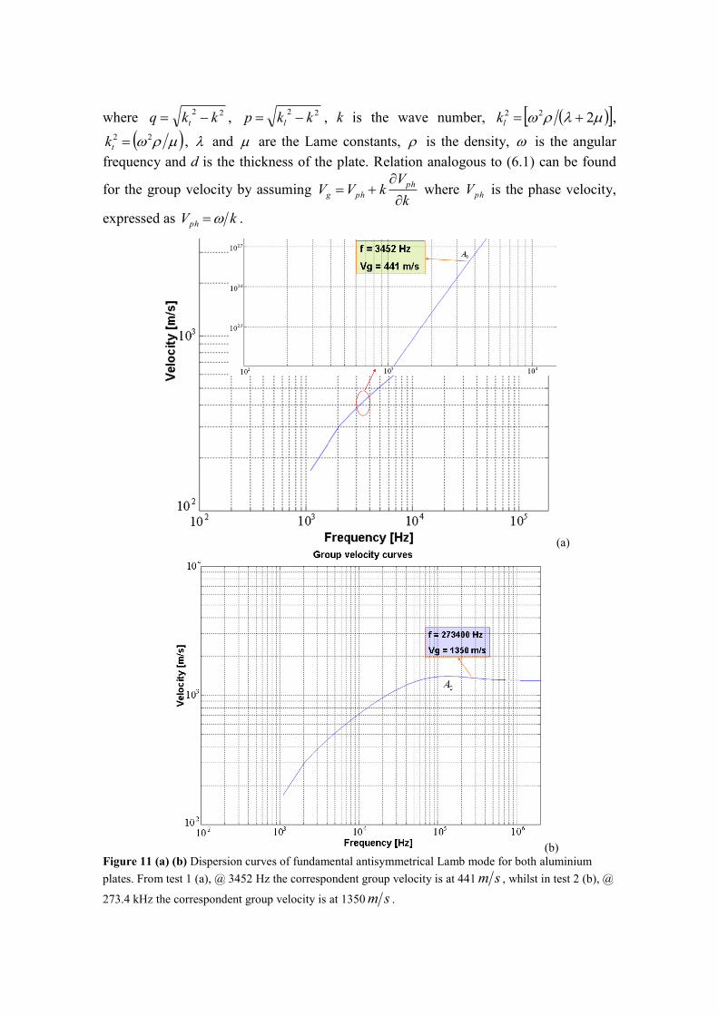
where 22kkq t , 22

kkp l , k is the wave number, 222 lk ,

22 tk , and are the Lame constants, is the density, is the angular

frequency and d is the thickness of the plate. Relation analogous to (6.1) can be found

for the group velocity by assuming k

VkVV

ph

phg

where phV is the phase velocity,

expressed as kVph .

(a)

(b) Figure 11 (a) (b) Dispersion curves of fundamental antisymmetrical Lamb mode for both aluminium

plates. From test 1 (a), @ 3452 Hz the correspondent group velocity is at 441 sm , whilst in test 2 (b), @

273.4 kHz the correspondent group velocity is at 1350 sm .

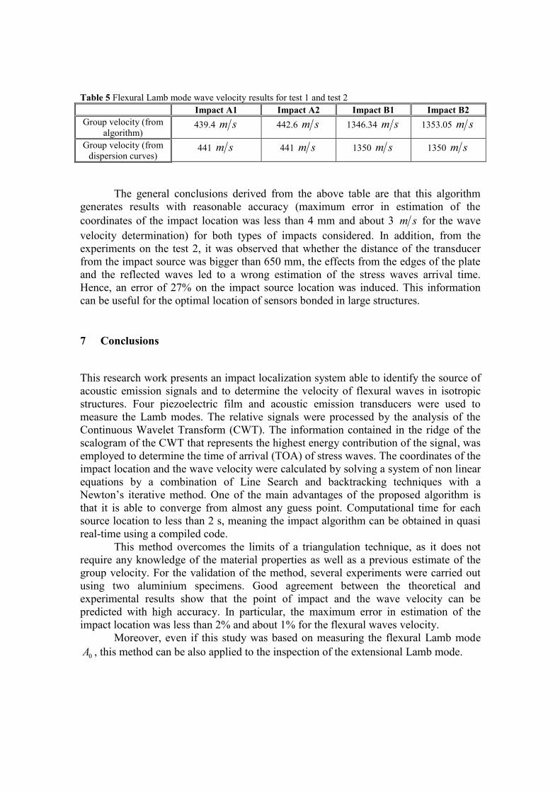
Table 5 Flexural Lamb mode wave velocity results for test 1 and test 2

Impact A1 Impact A2 Impact B1 Impact B2

Group velocity (from

algorithm) 439.4 sm 442.6 sm 1346.34 sm 1353.05 sm

Group velocity (from

dispersion curves) 441 sm 441 sm 1350 sm 1350 sm

The general conclusions derived from the above table are that this algorithm

generates results with reasonable accuracy (maximum error in estimation of the

coordinates of the impact location was less than 4 mm and about 3 sm for the wave

velocity determination) for both types of impacts considered. In addition, from the

experiments on the test 2, it was observed that whether the distance of the transducer

from the impact source was bigger than 650 mm, the effects from the edges of the plate

and the reflected waves led to a wrong estimation of the stress waves arrival time.

Hence, an error of 27% on the impact source location was induced. This information

can be useful for the optimal location of sensors bonded in large structures.

7 Conclusions

This research work presents an impact localization system able to identify the source of

acoustic emission signals and to determine the velocity of flexural waves in isotropic

structures. Four piezoelectric film and acoustic emission transducers were used to

measure the Lamb modes. The relative signals were processed by the analysis of the

Continuous Wavelet Transform (CWT). The information contained in the ridge of the

scalogram of the CWT that represents the highest energy contribution of the signal, was

employed to determine the time of arrival (TOA) of stress waves. The coordinates of the

impact location and the wave velocity were calculated by solving a system of non linear

equations by a combination of Line Search and backtracking techniques with a

Newton’s iterative method. One of the main advantages of the proposed algorithm is

that it is able to converge from almost any guess point. Computational time for each

source location to less than 2 s, meaning the impact algorithm can be obtained in quasi

real-time using a compiled code.

This method overcomes the limits of a triangulation technique, as it does not

require any knowledge of the material properties as well as a previous estimate of the

group velocity. For the validation of the method, several experiments were carried out

using two aluminium specimens. Good agreement between the theoretical and

experimental results show that the point of impact and the wave velocity can be

predicted with high accuracy. In particular, the maximum error in estimation of the

impact location was less than 2% and about 1% for the flexural waves velocity.

Moreover, even if this study was based on measuring the flexural Lamb mode

0A , this method can be also applied to the inspection of the extensional Lamb mode.

References

[1] Balageas D, Fritzen C P, Güemes A. “Structural Health Monitoring”. ISTE LTD,

2006

[2] Brown L F. “Disposable PVDF ultrasonic transducers for non-destructive testing

applications”. IEEE Transaction on Ultrasonics, Ferroelectrics, and Frequency

Control, Vol. 43, No. 3, 2000, pp. 560-568

[3] Dennis J E, Schnabel R B. “Numerical methods for unconstrained optimization and

non linear equations”. Soc. for Industrial & Applied Math., 1996

[4] El youbi F, Grondel S, Assaad J. “Signal processing for damage detection using two

different array transducers”. Ultrasonics 42, 2004, pp.803-806

[5] Gaul L, Hurlebaus S, Jacobs L J. “Localization of a “synthetic” acoustic emission

source on the surface of a fatigue specimen”. Research in Nondestructive

Evaluation, 2001, pp. 105-117

[6] Gaul L, Hurlebaus S. “Determination of the impact force on a plate by piezoelectric

film sensors”. Archive of Applied Mechanics, 69, 1999, pp. 691-701

[7] Giurgiutiu V. “Lamb wave generation with Piezoelectric Wafer Active Sensors for

structural health monitorig”. SPIE’s 10th Annual International Symposium on Smart

Structures and Material and 8th Annual International Symposium on NDE for

Health Monitoring and Diagnostics, San Diego, CA, 2002, paper # 5056-17, pp. 1-

12

[8] Haase M, Widjajakusuma J. “Damage identification based on ridges and maxima

lines of the wavelet transform”. International Journal of Engineering Science 41,

2003, pp. 1423-144

[9] Hamstad M A. “On Use of Piezoelectric Polymers As Wideband Acoustic Emission

Displacement Sensors for Composites". Proceedings of Fifth International

Symposium on Acoustic Emissions from Composite Materials (AECM-5), Sundsvall,

Sweden, The American Society for Nondestructive Testing, Inc., 1995, pp. 111-119.

[10] Hamstad M A, O’Gallagher A, Gary J. “A wavelet transform applied to acoustic

emission signals: Part 1: Source Identification”. Journal of Acoustic Emission, 20,

2002, pp. 39-61

[11] Jeong H, Jang Y-S. “Fracture source location in thin plates using the wavelet

transform of dispersive waves”. IEEE Transaction on Ultrasonics, Ferroelectrics,

and Frequency Control, Vol. 47, No. 3, 2000, pp.612-619

[12] Kim H, Melhem H. “Damage detection of structures by wavelet analysis”.

Engineering Structures, 26, 2004, pp. 347-362

[13] Kundu T, Das S, J K V. “Detection of the point of impact on a stiffened plate by

the acoustic emission technique”. Smart Materials and Structures 18, 2009, pp. 1-9

[14] Kosel T, Grabec I, Kosel F. “Intelligent location of simultaneously active

acoustic emission sources”. Aircraft Engineering and Aerospace Technology, Vol.

75, No. 1, 2003, pp. 11-17

[15] Le T-P, Argoul P. “Continuous wavelet transform for modal identification using

free decay response”. Journal of Sound and Vibration 277, 2004, pp. 73-100

[16] Mallat S. “A wavelet tour of signal processing”. London: Academic Press, 1998

[17] Meo M, Zumpano G, Pigott M, Marengo G. “Impact identification on a

sandwich plate from wave propagation responses”. Composite Structures 71, 2005,

pp. 302-306

[18] Monkhouse R S C, Wilcox P W, Lowe M J S, Dalton R P, Cawley P. “The rapid

monitoring of structures using interdigital Lamb wave transducers”. Smart Materials

and Structures 9, 2000, pp. 753-780

[19] Nocedal J, Wright S J. “Numerical Optimization”. Springer Series in Operations

Research, 1999

[20] Paget C A, Atherton K, O’Brien E. “Triangulation algorithm for damage

location in aeronautical composite structures”. Proceeding of the 4th International

Workshop on Structural Health Monitoring, Stanford, CA, 2003, pp. 363-370

[21] Reddy J N. “Theory and analysis of elastic plates”. Taylor & Francis LTD, 1999

[22] Seydel R, Chang F K. “Impact identification on stiffened composite panels:

system development”. Smart Materials and Structures 10, 2001, pp. 354-369

[23] Sung D U, Oh J H, Kim C G, Hong C S. “Impact monitoring of smart composite

laminates using neural network and wavelet analysis”. Journal of Intelligent

Material Systems, Vol. 11, 2000, pp. 180-190

[24] Tobias A. “Acoustic emission source location in two dimensions by an array of

three sensors”, Non-Destructive Testing, Vol. 9, No. 1, 1976, pp. 9-12

[25] Viktorov I A. “Rayleigh and Lamb waves. Physical theory and applications”.

Plenum Press New York, 1967

[26] Ziola S M, Gorman M R. “Source location in thin plates using cross-

correlation”. The Journal of the Acoustic Society of America 90 (5), 1991, pp. 2551-

2556