Embed Size (px)
Citation preview

Mémoire présenté
devant l’Institut de Science Financière et d’Assurances
pour l’obtention du diplôme d’Actuaire de l’Université de Lyon
le 7 Juin 2013
Par : Rudy J. Daccache
Titre: Interest Rate Dynamics in the Lebanese Market
Confidentialité : NON OUI (Durée : 1 an 2 ans)
Membres du jury de l’Institut des Actuaires
Entreprise :
Group Risk Management – Bank Audi,
Lebanon
Membres du jury I.S.F.A. Directeur de mémoire en entreprise :
Mme Flavia BARSOTTI Adel N. Satel
M. Alexis BIENVENÜE
M. Areski COUSIN Invité :
Mme Diana DOROBANTU
Mme Anne EYRAUD-LOISEL
M. Nicolas LEBOISNE
M. Stéphane LOISEL Autorisation de mise en ligne sur
un site de diffusion de documents
actuariels (après expiration de
l’éventuel délai de confidentialité)
Mlle Esterina MASIELLO
Mme Véronique MAUME-DESCHAMPS
M. Frédéric PLANCHET
Mme
M.
Béatrice REY-FOURNIER
Pierre RIBEREAU
M. Christian-Yann ROBERT Signature du responsable entreprise
M.
M.
Didier RULLIERE
Pierre THEROND
Secrétariat Signature du candidat
Mme Marie-Claude MOUCHON
Bibliothèque :
Mme Patricia BARTOLO
50 Avenue Tony Garnier 69366 Lyon Cedex 07
Université Claude Bernard – Lyon 1
INSTITUT DE SCIENCE FINANCIERE ET D'ASSURANCES


Graduate School of Actuarial StudiesClaude Bernard University, Lyon
&
Group Risk Analytics and Integration DepartementBank Audi, Beirut
Actuarial Thesis
Interest Rate Dynamics in theLebanese Market
Author:Rudy Daccache
Supervisor:Christian Robert
Disclaimer: This Actuarial Thesis should not be reported as representing the viewsof Bank Audi. The views expressed in this Thesis are those of the author and do notnecessarily represent those of Bank Audi or Bank Audi policy. The consequences ofany action taken on the basis of information contained herein are solely the respons-ibility of the recipient.
May, 2013


Interest Rate Dynamics in the Lebanese Market Actuarial Thesis
Executive Summary
Interest rate risk is one of the most important risk in managing fixed income portfolio orthe whole balance sheet of a bank. In this work, we aim to study the dynamics of interestrates in the Lebanese market. In the first part, we study the yield curve obtained fromthe observed rates of bonds issued by the Lebanese Government in Local Currency andin US dollar, whereas in the second part we aim to identify the impact of Market interestrates shocks on US dollar deposit rate offered by Lebanese Banks.
Part I
The objective of the first part is to build the Lebanese term-structure of interest ratesbased on bonds issued by the Lebanese Government in local currency and US dollar.This model can be used for risk management and plays an important role in pricing fixed-income securities and interest rate derivatives, as well as other financial assets. Since zerocoupon rates are not observable for a range of maturities, an estimation methodology isrequired to derive the zero coupon yield curves from observable data.After reviewing articles related to the topics and seeing models used by central banks,we decided to apply Nelson Siegel Model and its extension proposed by Svensson. Lot ofpapers highlighted difficulties found in estimating the parameters specifically in Svenssonmodel due to the number of coefficients to be estimated relative to the limited set ofobservable yields on the secondary market.For this issue, we have collected historical prices of Lebanese government bonds from 2009until January 2013, since earlier data is not available on Bloomberg platform. Then weapplied the bootstrapping method to obtain exact zero yields.Turning to the two models, we applied various parameters estimation methods and wedefined a new method for the estimation called ”Correlation Constraint Approach” inwhich a new constraint has been added to maintain a small correlation between the load-ing factors. Nevertheless, this approach guided to obtain more stable parameters thatchanges in response to any remarkable regional political or economical situation change.During the last four years, there was many changes in the economical and political situ-ations. These events are reflected in our results by a regime switching model applied onestimated parameters. Therefore, any change in the situation will be helpful in forecastingthe Lebanese term-structure. Moreover, an economic expert opinion can be added to themodel for prediction.
Part II
Traditional customer deposits are the main funding source of Lebanese commercial banks(80-85% of liabilities). Although they are contractually short term (mainly one month)paying fixed interest rates, these deposits are historically known to be a stable source offunding and therefore exhibit a sticky behavior to changes in market interest rates.This sticky behavior gives Lebanese banks a high bargaining power to control the pass-through of market shocks and therefore control their sensitivity to interest rates.
2

Interest Rate Dynamics in the Lebanese Market Actuarial Thesis
In this paper we modeled the behavioral versus contractual repricing of customer deposits.In other words, we measured the real impact of interest rate shocks on the bank’s profitsand economic value of shareholders’ equity.For this matter, we have gathered interest rate data from 2003 until the end of 2011since earlier data is no longer relevant to the actual state of the banking sector and theLebanese economy in general. We used LIBOR as a proxy for market interest rates andthe Banking Sector Average Rate as a proxy for interest rates paid by Lebanese banks oncustomer deposits.After reviewing the literature concerning this subject and applying different econometricmodels, we came to the conclusion that an Error Correction Model (ECM) is the mostappropriate to reach the results we are aiming for.Within this ECM framework, we were able to identify the short and long run pass-throughrates in response to interest rate shocks. In addition, we formulated an impulse responsefunction that will measure the speed, in months, it would take a shock to be transmittedto rates paid on deposits.Results showed that 6.8% of a market shock will be passed-through immediately whilethe final pass-through rate is 33%.These results would make it possible to determine the effective duration (repricing date)of customer deposits when market interest rates fluctuate.A positive shock in interest rates, which is the standard stress test used to measurebanks’ sensitivity to interest rates, will usually yield a negative impact as assets’ durationis higher than liabilities’ duration.When considering the results of our model, the effective duration of liabilities will behigher than the contractual one which will lower the duration gap between assets andliabilities and thus the negative impact of positive interest rate shocks.
Keywords: Interest rate risk, Nelson-Siegel, Nelson-Sigel-Svensson, Time Series Analy-sis, Error Correction Model, Impulse Response Function.
3

Interest Rate Dynamics in the Lebanese Market Actuarial Thesis
Resume
Le risque de taux d’interet est l’un des risques les plus importants dans la gestion desportefeuilles des obigations a revenu fixe ou en general dans la gestion actif-passif d’unebanque. Dans ce travail, nous visons a etudier la dynamique des taux d’interet au Liban.Dans la premiere partie, nous etudions la courbe des taux obtenue a partir des tauxobserves sur le marche secondaire des obligations emises par le gouvernement libanaisen Livres Libanaises et en Dollar Americain. Dans la deuxieme partie nous etudionsl’impact des chocs dans le marche des taux d’interets internationaux sur le taux verse parles banques libanaises sur les depots en Dollar Americain.
Partie 1
L’objectif de cette partie est de construire la courbe des taux d’interet a partir des obli-gations emises par le gouvernement libanais en monnaie locale et en dollar americain.Ce modele peut etre utilise pour la gestion des risques et joue un role important dansl’etablissement de prix des titres a revenu fixe et des produits derives des taux interet,ainsi que d’autres actifs financiers. Puisque les taux des obligations a coupon zero nesont pas observes pour toutes les echeances, une construction de la courbe de taux estnecessaire pour avoir ces taux.Apres une recherche sur le sujet et sur les modeles utilises par les banques centrales, nousavons decide d’appliquer le modele de Nelson-Siegel et celui de Svensson. Plusieurs arti-cles de recherche mettent en relief les difficultes dans l’estimation des parametres surtoutdans le modele de Svensson puisque le nombre des parametres a estimer est grand parrapport au nombre des points observes.Pour cette question, nous avons collecte les donnees historiques des prix des obligationsemises par le gouvernement libanais pour la periode allant de 2009 jusqu’a Janvier 2013puisque les donnees anterieures ne sont pas disponible sur Bloomberg.Pour l’estimation des parametres, nous avons utilise plusieurs methodes et nous avonsdefini une nouvelle methode appelee “Approche par contrainte de correlation” dans laque-lle nous avons introduit une nouvelle contrainte dans le probleme d’optimisation pourmaintenir une petite correlation entre les facteurs. La nouvelle approche a donne desparametres plus stables et changeant de regime comme une reponse a un changementdans la situation economique ou politique dans le pays ou bien dans la region du moyen-orient.Donc, nous avons obtenu des parametres qui peuvent-etre interpretes economiquementpar des changements dans la situation libanaise ou regionale. Une opinion d’un experteconomique pour la prdiction doit etre prise en consideration dans le modele.
Partie 2
Les depots des clients traditionnels sont la source principale de financement des ban-ques commerciales Libanaises (80-85 % des engagements). Bien qu’ils soient contractuelsa court terme (principalement un mois) obtenant des taux d’interet fixes, ces depotssont historiquement connus pour etre une source de financement stable, donc ils ont un
4

Interest Rate Dynamics in the Lebanese Market Actuarial Thesis
comportement moins variable aux changements des taux d’interet dans les marches inter-nationaux.Ce comportement moins variable donne aux banques libanaises un pouvoir de jouer surla sensibilite aux taux d’interet.Dans ce travail, nous avons modelise la reevaluation des depots en se basant sur le com-portement contractuel et le comportement ajuste. En d’autres termes, nous avons mesurel’impact reel de chocs dans les taux d’interet internationaux sur les benefices de la banqueet de la valeur economique des capitaux propres.Pour cette question, nous avons recueilli des donnees historiques de taux d’interet a partirde 2003 et jusqu’a la fin de 2011, car les donnees avant 2003 ne sont plus pertinentes al’etat actuel du secteur bancaire et de l’economie libanaise en general. Nous avons con-sidere le LIBOR comme un indicateur indirect des taux d’interet internationaux et leBanking Sector Average Rate (BSAR) comme un proxy de taux d’interet moyen paye parles banques libanaises sur les depots des clients en dollar americain.Apres avoir examine la litterature sur ce sujet et en appliquant differents modeles econom-etriques, nous avons conclu que le modele a correction d’erreur (MCE) est le plus appro-prie pour atteindre notre objective.Le MCE nous aide a identifier le pass-through des taux comme une reponse aux chocs d’unautre taux d’interet a court et long terme. En outre, nous avons formule une fonction dereponse impulsionnelle qui permettra de mesurer la vitesse de la propagation du choc enmois pour etre transmis au taux paye sur les depots libanais en dollar americain.Les resultats ont montre que 6,8% d’un choc de LIBOR sera absorbe immediatement parle taux libanais alors qu’a la fin il va absorber 33% au total.Ces resultats permettraient de determiner la duree effective (Dates de revalorisation) desdepots de la clientele lorsque les taux d’interet du marche fluctuent.Un choc positif dans les taux d’interet, ce qui est le stress test normal utilise pour mesurerla sensibilite des banques au changement dans les taux d’interet, a habituellement donneun impact negatif puisque la duree des actifs est superieur au celle des engagements.Lorsqu’on considere les resultats de notre modele, la duree effective du passif sera pluselevee que celle contractuelle, et cela conduit a baisser l’ecart de duration entre les actifset les passifs et a un impact negatif sur le capital requis.
Mots cles: Risque des taux, Nelson-Siegel, Nelson-Sigel-Svensson, Analyse des seriestemporelles, Modele a correction d’erreur, Fonction de reponse impulsionnelle.
5

Interest Rate Dynamics in the Lebanese Market Actuarial Thesis
Acknowledgement
First, I would like to express my sincere gratitude to my supervisor Christian Robert forhis continuous support of my PhD. His guidance and comments were instrumental to myresearch and writing of this thesis.
I would like to also thank Mr. Adel Satel, Group Chief Risk Officer at Bank Audi-Lebanon, who gave me the opportunity to undertake my PhD at ISFA, Claude BernardUniversity-Lyon.
My sincere thanks go to Chadi Nawar, a colleague at Bank Audi, for his insight through-out this project.
I thank members of the Mathematics Department at Saint Joseph University-Beirut, fortheir ongoing support since 2008 and all my colleagues at the risk management depart-ment of Bank Audi and the research laboratory of ISFA, Claude Bernard University-Lyonfor their help and encouragement.
Last but not the least, I would like to thank my family: my parents, my brother andhis wife for supporting every choice I made.
6

Interest Rate Dynamics in the Lebanese Market Actuarial Thesis
7

Contents
Introduction 12
1 Interest Rate Risk Management 141.1 Definition of interest rate risk . . . . . . . . . . . . . . . . . . . . . . . . . 141.2 The management of Net Interest Income . . . . . . . . . . . . . . . . . . . 15
1.2.1 Duration . . . . . . . . . . . . . . . . . . . . . . . . . . . . . . . . . 151.2.2 Convexity . . . . . . . . . . . . . . . . . . . . . . . . . . . . . . . . 161.2.3 Principal Component Analysis . . . . . . . . . . . . . . . . . . . . . 16
Part I: Building The Lebanese Term-Structure 18
2 Zero-Coupon Yield Curves 182.1 Introduction . . . . . . . . . . . . . . . . . . . . . . . . . . . . . . . . . . . 182.2 Theoretical Background . . . . . . . . . . . . . . . . . . . . . . . . . . . . 18
2.2.1 Bootstrapping Method . . . . . . . . . . . . . . . . . . . . . . . . . 192.2.2 Cubic-Spline Method . . . . . . . . . . . . . . . . . . . . . . . . . . 202.2.3 Merrill Lynch Exponential Spline . . . . . . . . . . . . . . . . . . . 212.2.4 Nelson-Siegel Model . . . . . . . . . . . . . . . . . . . . . . . . . . 222.2.5 Nelson-Siegel-Svensson Model . . . . . . . . . . . . . . . . . . . . . 25
2.3 Zero-coupon yield curves in central banks . . . . . . . . . . . . . . . . . . . 26
3 Lebanese Yield Curve 283.1 Introduction . . . . . . . . . . . . . . . . . . . . . . . . . . . . . . . . . . . 283.2 Data . . . . . . . . . . . . . . . . . . . . . . . . . . . . . . . . . . . . . . . 283.3 Estimation Methods . . . . . . . . . . . . . . . . . . . . . . . . . . . . . . 293.4 Application . . . . . . . . . . . . . . . . . . . . . . . . . . . . . . . . . . . 31
3.4.1 Nelson-Siegel Applied on the USD Yield Curve . . . . . . . . . . . 333.4.2 Nelson-Siegel Applied on the LBP Yield Curve . . . . . . . . . . . . 353.4.3 Nelson-Siegel-Svensson Applied on the USD Yield Curve . . . . . . 373.4.4 Nelson-Siegel-Svensson Applied on the LBP Yield Curve . . . . . . 393.4.5 Conclusion . . . . . . . . . . . . . . . . . . . . . . . . . . . . . . . . 41
3.5 Lebanese Yield Curves Movements . . . . . . . . . . . . . . . . . . . . . . 423.6 Economical Interpretation . . . . . . . . . . . . . . . . . . . . . . . . . . . 453.7 Conclusion . . . . . . . . . . . . . . . . . . . . . . . . . . . . . . . . . . . . 47
8

Interest Rate Dynamics in the Lebanese Market Actuarial Thesis
Part II: Modeling the impact of Libor on US deposit offeredrate 50
4 Vector Autoregression and Error Correction Model 504.1 Introduction . . . . . . . . . . . . . . . . . . . . . . . . . . . . . . . . . . . 504.2 Statistical Background . . . . . . . . . . . . . . . . . . . . . . . . . . . . . 50
4.2.1 Stationarity . . . . . . . . . . . . . . . . . . . . . . . . . . . . . . . 504.2.2 Granger Causality Test . . . . . . . . . . . . . . . . . . . . . . . . . 524.2.3 Lag Length Criteria . . . . . . . . . . . . . . . . . . . . . . . . . . . 524.2.4 Jarque-Bera Test . . . . . . . . . . . . . . . . . . . . . . . . . . . . 534.2.5 Cointegration . . . . . . . . . . . . . . . . . . . . . . . . . . . . . . 54
4.3 VAR Model . . . . . . . . . . . . . . . . . . . . . . . . . . . . . . . . . . . 574.3.1 Definition . . . . . . . . . . . . . . . . . . . . . . . . . . . . . . . . 574.3.2 Order of Integration . . . . . . . . . . . . . . . . . . . . . . . . . . 574.3.3 Stability of the VAR model . . . . . . . . . . . . . . . . . . . . . . 574.3.4 Impulse Response Function . . . . . . . . . . . . . . . . . . . . . . 58
4.4 VEC Model . . . . . . . . . . . . . . . . . . . . . . . . . . . . . . . . . . . 594.4.1 Definition . . . . . . . . . . . . . . . . . . . . . . . . . . . . . . . . 594.4.2 Interpretation of the coefficients . . . . . . . . . . . . . . . . . . . . 59
5 Pass-Through of Interest Rate Shocks to Lebanese Deposit Rates 625.1 Introduction . . . . . . . . . . . . . . . . . . . . . . . . . . . . . . . . . . . 625.2 Data . . . . . . . . . . . . . . . . . . . . . . . . . . . . . . . . . . . . . . . 62
5.2.1 Banking Sector Average Rate (BSAR) . . . . . . . . . . . . . . . . 635.2.2 London InterBank Offered Rate (LIBOR) . . . . . . . . . . . . . . 635.2.3 Descriptive statistics of the two variables . . . . . . . . . . . . . . . 64
5.3 Error Correction model . . . . . . . . . . . . . . . . . . . . . . . . . . . . . 655.3.1 Definition . . . . . . . . . . . . . . . . . . . . . . . . . . . . . . . . 655.3.2 Model Results . . . . . . . . . . . . . . . . . . . . . . . . . . . . . . 66
5.4 Shock Analysis . . . . . . . . . . . . . . . . . . . . . . . . . . . . . . . . . 675.5 Application . . . . . . . . . . . . . . . . . . . . . . . . . . . . . . . . . . . 685.6 Conclusion . . . . . . . . . . . . . . . . . . . . . . . . . . . . . . . . . . . . 70
6 Conclusion 72
Bibliography 74
A Fixed Income Portfolio Example 76
B Yield Curve Models in Central Banks 78
C Principal Component Analysis Tables 80
D Stationarity Tools 82D.1 A unit root process has a variance that depends on time . . . . . . . . . . 82D.2 If a process has a unit root then the process will be non-stationary . . . . . 82
9

Interest Rate Dynamics in the Lebanese Market Actuarial Thesis
D.3 Student’s T-test . . . . . . . . . . . . . . . . . . . . . . . . . . . . . . . . . 83
E Cointegration and ECM Tools 84E.1 If the vector Xt has two components therefore the number of linearly in-
dependent cointegrating vectors will be at most equal to one . . . . . . . . 84E.2 Transformation of a simple VAR model to VECM . . . . . . . . . . . . . . 86E.3 Johansen Procedure . . . . . . . . . . . . . . . . . . . . . . . . . . . . . . . 86E.4 If N variables can be written in N linearly independent stationary equations,
then the N variables are stationary. . . . . . . . . . . . . . . . . . . . . . . 87
F Error Correction Model Application’s Tools 88F.1 Transformation of ADL(1,1) model to VEC model . . . . . . . . . . . . . . 88F.2 Impulse Response Function . . . . . . . . . . . . . . . . . . . . . . . . . . 88F.3 GAP Analysis . . . . . . . . . . . . . . . . . . . . . . . . . . . . . . . . . . 89
10

Interest Rate Dynamics in the Lebanese Market Actuarial Thesis
11

Interest Rate Dynamics in the Lebanese Market Actuarial Thesis
Introduction
Modeling and forecasting interest rate dynamics is of great importance in many areasof finance such as derivatives pricing, asset allocation and debt restructuring. Not sur-prisingly, a vast amount of literature is devoted to research in this part of academia inorder to find optimal methods to estimate and to forecast the term-structure of interestrates.
In this thesis, we concentrate on the Lebanese Market since this work is helpful for BankAudi-Beirut in managing market risks basing on advanced econometric models. The de-velopment was done in parallel with my work on the PhD thesis at the bank and at theresearch laboratory of ISFA, Claude Bernard University-Lyon. The literature of existingmodels is explained in the introduction of each chapter.
Before outlining the developed parts, we are interested in providing a historical review forthe Lebanese Economy between 1950 and 1995 to show how Lebanon is trying to enterglobal markets by maintaining a fixed exchange rate between the domestic currency andthe US dollar.
Lebanon has always been known as the Switzerland of the Middle-East mainly due toits first class banking services benefiting from a banking secrecy law that was passed in1956. Beirut, its capital, is regarded as Paris of the East with all the touristic facilities itoffers.
Until 1950, the Lebanese economy relied essentially on the exportation of agriculturalproducts. Unfortunately, in 1975, the Lebanese civil war erupted and lasted until 1990destroying the infrastructure and paralyzing the economic activity. Lebanon started los-ing gradually its status as ”Switzerland of the Middle-East”. Moreover, after the civilwar, economic problems persisted and led to an actual public debt near 56 billion USDand representing 137% of the country’s GDP.
During the civil war, the worst period for the Lebanese economy was between 1982 and1988. The Israeli invasion caused a chaos in the country. Deposits in Lebanese Banksdecreased, in value, from 12 Billion USD in 1982 to 3.5 Billion USD in 1988 due to a de-preciation of the Lebanese pound that went from 4.5 pounds per US dollar to 500 poundsbefore stabilizing at a level between 800 to 1000 pounds. The country, emerging from fif-teen years of violence, had a damaged infrastructure and 600’000 people displaced whichaffected the productive capacity of the economy. In addition, the Israeli army occupieda large part of Southern Lebanon until 2000. Reconstruction of the infrastructure costaround 3.5 Billion USD. Thus, the country was facing a difficult situation and the deteri-oration of the currency continued until it touched 2800 pounds per US dollar in summer1992.
Since 1992, Lebanon is trying to regain its post war status and to enter global mar-kets. Between 1995 and 1996, the Lebanese pound was pegged against the US dollar at
12

Interest Rate Dynamics in the Lebanese Market Actuarial Thesis
an average fixed rate of 1507.5 USD/LBP. The fixed exchange rate was the first step ofthe Lebanese Central Bank strategy to regain local and international investors confidence.This led to a monetary policy in Lebanon highly influenced by the US monetary policy.
The rest of the thesis is organized as follows. In the first chapter, we give a generalintroduction to interest rate risk management in Banks. Chapter 2 provide an overviewof the different models employed in building the term structure of zero yields as well asthe used models in top world central banks. In chapter 3, we develop a new estimationmethod called ”Correlation Constraint approach” which can be applied on Nelson-SiegelModel and it extension proposed by Svensson, also we estimate the Lebanese Governmentterm-structure of zero yields denominated in LBP and USD currency then we study theevolution of the parameters in order to identify interest rate dynamics which is explainedin the end of the chapter by an eco-political interpretation. On the other hand, in thefollowing two chapters, we model the impact of changes in market interest rates on theoffered rate by Lebanese Banks on USD deposits. Chapter 4 provides the theoreticalbackground behind the model applied in chapter 5.
13

Chapter 1
Interest Rate Risk Management
1.1 Definition of interest rate risk
Interest rate risk is the exposure of a bank’s financial condition to adverse movementsin interest rates. Banks accept this risk since it’s the main source of profitability andshareholder value. Fluctuations in interest rates cause changes in the net interest incomeof banks also in other interest-sensitive income and operating expenses. Nevertheless, theunderlying value of the bank’s assets, liabilities and off-balance-sheet instruments can beaffected by changes in interest rates since the present value of future cash flows changewhen interest rates change. Before setting out how to measure this risk, we provide abrief introduction to the sources of interest rate risk. (c.f. BASEL - Principles for themanagement and supervision of Interest Rate Risk.)
Sources of Interest Rate Risk:
Repricing Risk. The repricing risk arises from timing differences in the maturityfor fixed-rate instruments and repricing for floating-rate instruments. For instance,the income of a loan with a variable rate will increase when rates rise and decreaseswhen rates fall, whereas if the loan is funded with fixed rated deposits, the bank’sinterest margin will fluctuate.
Yield Curve Risk. The yield curve risk originates from the spread between short-term and long-term interest rates. For instance, the underlying economic value ofa long position in 10-year government bonds hedged by a short position in 5-yearbond government notes could decline sharply if the yield curve steepens, even if theposition is hedged against parallel movements in the yield curve.
Basis Risk. The basis risk arises from imperfect correlation in the adjustment ofthe rates earned and paid on different instruments with otherwise similar repricingcharacteristics. For example, a plan of funding of a one-year loan that repricesmonthly based on 1 month US LIBOR rate with a one-year deposit that reprices
14

Interest Rate Dynamics in the Lebanese Market Actuarial Thesis
monthly based on 1 Month US Treasury Bills, exposes the bank to the risk that thespread between the two index rates may change unexpectedly.
Option Risk. The option risk originates from the options embedded in many bankassets, liabilities, and off-balance sheet portfolios. In other words, mortgage loanspresent significant option risk due to prepayment speeds that change dramaticallywhen interest rates rise and fall. For example, borrowers will refinance and repaytheir loans and leave the bank with uninvested cash when interest rates have de-clined. Alternately, rising interest rates cause mortgage borrowers to repay slower,leaving the bank with more loans based on prior, lower interest rates.
In the following, we provide a brief summary for modeling the interest rate risk.
1.2 The management of Net Interest Income
The net interest income of a bank is defined as the excess of interest received over interestpaid. The asset-liability management unit takes the charge of ensuring that net interestincome remains roughly through time. One way of doing this job is to ensure that thematurities of the assets on which interest is earned and the maturities of the liabilities onwhich interest is paid are matched. Referring to the liquidity preference theory, long-termrates should be higher than short-term rates.
1.2.1 Duration
Duration is a widely used measure of a portfolio’s exposure to yield curve movements.Suppose y is a bonds yield and B is its market price. The duration D of the bond is givenby
∆B
B= −D∆y
where ∆y is a small change in the bond’s yield and ∆B is the corresponding change inits price. Duration measures the sensitivity of percentage changes in the bond’s price tochanges in its yield. Using calculus notation, we can write
D = − 1
B
dB
dy
We consider a bond that provides cash flows c1, c2, · · · , cn at times t1, t2, · · · , tn. Thenthe price of the bond is defined by the following formula:
B =n∑i=1
ci exp(−yti)
From this, it follows that
D =n∑i=1
ti
(ci exp(−yti)
B
)Thus, the duration is a weighted average of the times when payments are made, with theweight applied to time ti being equal to the proportion of the bond’s total present valueprovided by the cash flow at time ti.
15

Interest Rate Dynamics in the Lebanese Market Actuarial Thesis
1.2.2 Convexity
The duration relationship measures exposure to small changes in yields. We introducea factor known as convexity which improves the relationship between bond prices andyields. The convexity for a bond is:
C =1
B
d2B
dy2=
∑ni=1 cit
2i exp(−yti)B
Therefore the second-order approximation to change in the bond price is:
∆B
B= −D∆y +
1
2C(∆y)2
We illustrate the importance of the convexity in Appendix A.
1.2.3 Principal Component Analysis
Principal Component Analysis is a statistical technique in which the original variables arereplaced by a smaller number of artificial variables that preserve as much as possible of thevariability of the original variables. In other words, PCA guide us to reduce the numberof the variables and to detect a structure in the relationships between the variables. Weimplement this method to build the structure between different yields used to build yieldcurve. We take weekly changes in France Eurobond Yields to identify the behavior ofthe yield curve and factor loadings from France Eurobond Yields are represented in thetable 1.1.We represented the first ten factors describing the rate moves. The first factor, shown in
Table 1.1: Factor Loadings for EUR France Eurobond Yields
PC1 PC2 PC3 PC4 PC5 PC6 PC7 PC8 PC9 PC10
3M -0.28 0.49 -0.24 -0.20 0.26 -0.10 0.31 -0.10 0.01 -0.266M -0.29 0.49 -0.21 -0.16 0.01 -0.11 0.11 -0.04 0.22 0.221Y -0.30 0.39 -0.10 0.23 -0.30 0.23 -0.61 0.29 -0.28 0.072Y -0.30 0.09 0.34 0.71 -0.17 0.11 0.28 -0.33 0.18 -0.093Y -0.31 -0.03 0.47 0.08 0.48 -0.41 0.02 0.28 -0.42 0.154Y -0.28 -0.11 0.31 -0.18 0.16 0.09 -0.29 0.29 0.72 -0.165Y -0.28 -0.11 0.22 -0.36 0.02 0.25 -0.16 -0.56 -0.11 0.366Y -0.28 -0.15 0.11 -0.26 -0.08 0.24 0.04 -0.16 -0.15 -0.087Y -0.27 -0.18 0.00 -0.16 -0.19 0.24 0.25 0.23 -0.20 -0.518Y -0.26 -0.20 -0.09 -0.09 -0.26 -0.02 0.22 0.23 -0.13 -0.049Y -0.25 -0.22 -0.19 -0.03 -0.32 -0.28 0.14 0.05 0.04 0.35
10Y -0.23 -0.25 -0.20 0.06 -0.21 -0.39 -0.03 0.04 0.20 0.1715Y -0.19 -0.22 -0.31 0.11 0.18 -0.31 -0.42 -0.39 -0.09 -0.4520Y -0.15 -0.21 -0.33 0.22 0.30 0.14 -0.02 -0.03 0.05 0.0430Y -0.13 -0.20 -0.34 0.20 0.42 0.46 0.14 0.18 0.00 0.29
16

Interest Rate Dynamics in the Lebanese Market Actuarial Thesis
the column labeled PC1, corresponds to a roughly parallel shift in the yield curve. Whenwe have one unit of that factor, the three-month rate increases 0.28, the 6-month rate0.29 and so on. The second factor is shown in column labeled PC2. It corresponds to atwist or change of slope of the yield curve. Rates between 3 months and 2 years move inone direction; rates between 3 years and 30 years move in the other direction. The thirdfactor corresponds to a “bowing” of the yield curve. Rates at the short end and long endof the yield curve move in one direction; rates in the middle move in other direction.The importance of each factor is measured by the standard deviation of its factor score.
Table 1.2: Standard Deviation of factor scores
PC1 PC2 PC3 PC4
Standard Deviation 1.729593 0.858561 0.440685 0.191791Proportion of Variance 74.31% 18.31% 4.82% 0.91%Cumulative Proportion 74.31% 92.62% 97.45% 98.36%
We represent standard deviations of the factor scores in the table 1.2. The table showsthat the first factor accounts for 74.31% of the variance and the most three importantfactors accounts for 97.45% of the variance.We illustrate the importance of the PCA by an example. We suppose that an investor hold
Table 1.3: Change of portfolio value for a 1 basis point rate move
Rate 1Y 2Y 3Y 4Y 5Y
Change 15 9 -10 -17 1
a large portfolio and we represent the exposures to interest rate moves in the table 1.3, a1 basis point change in the one-year rate causes the portfolio to increase by $15 million; a1 basis point change in the two-years rate causes it to increase by $9 million dollars; andso on. We use the first two factors to model rate moves:
FACTOR 1
0.3× 15 + 0.3× 9 + 0.31×−10 + 0.28×−17 + 0.28× 1 = −0.52
FACTOR 2
−0.39× 15− 0.09× 9 + 0.03×−10 + 0.11×−17 + 0.11× 1 = −8.73
The results provides us that the exposure of the portfolio to the second shift is about 17times greater than the exposure to the first shift. However, the first shift is about fourtimes as important in terms of the extent to which it occurs.
17

Chapter 2
Zero-Coupon Yield Curves
2.1 Introduction
The relationship between the yields of default-free zero coupon bonds and their length tomaturity is defined as the term structure of interest rates and is shown pictorially in theyield curve. This relation can be used for risk management and has an important rolein pricing fixed-income securities and interest rate derivatives, as well as other financialassets. Because of its numerous uses, an accurate estimate of the term structure hasconstituted a major question in the empirical literature in economics and finance.There are two distinct approaches to estimate the term structure of interest rates: theequilibrium models and the statistical techniques. Examples of the first approach includeVasicek (1977), Dothan (1978), Brenan and Schwartz (1979), Cox and Ingersoll Ross(1985) and Duffie and Kan (1996). These models are formalized by defining state variablescharacterizing the state of the economy which are driven by these random processes andare related in some way to the prices of bonds. It then uses no-arbitrage arguments toinfer the dynamics of term structure. In contrast to equilibrium models, the statisticaltechniques focusing on obtaining a continuing yield curve from cross-sectional couponbond data based on curve fitting techniques are able to describe a richer variety of yieldpatterns in reality. The most known models employed in the second approach are Nelson-Siegel(1987) and its extension by Svensson (1994).Most central banks use either the Nelson-Siegel or the extended version suggested bySvensson (see e.g. Appendix B). Exceptions are Canada, Japan, Sweden, the UnitedKingdom, and the United States of America which all apply variants of the smoothingsplines method. They employ government bonds in the estimations since they carry nodefault risk.
2.2 Theoretical Background
The spot interest rate of a given maturity m is defined as the yield on a pure discountbond of that maturity. The spot rates are discount rates determining the present valueof a unit payment at a given time in the future. Spot rates considered as a function ofmaturity are referred to as the term-structure of interest rates.
18

Interest Rate Dynamics in the Lebanese Market Actuarial Thesis
The value of a coupon bond is simply the present value of the stream of future cash flowsit provides. That is,
B =T∑
m=1
CFm(1 +R(m))m
where T denotes the maturity of the bond, CFm is the cash flow paid by the bond at timem = 1, · · · , T and R(m) is referred to as the spot interest rate for maturity m years.In the following, our objective is to estimate zero-coupon rates, or forward rates, ordiscount functions from a set of coupon bond prices. Generally this requires fitting aparsimonious functional form that is flexible in capturing stylized facts regarding theshape of the term structure. A good term structure estimation method should satisfy thefollowing requirements:
• The method ensures a suitable fitting of the data.
• The estimated zero-coupon rates and the forward rates remain positive over theentire maturity spectrum.
• The estimated discount functions, and the term structures of zero coupon rates andforward rates are continuous and smooth.
• The method allows asymptotic shapes for the term structures of zero-coupon ratesand forward rates at the long end of the maturity spectrum.
In the following, we focus on five commonly used term structure estimation methodsgiven as the bootstrapping method, the cubic-spline, Merrill Lynch exponential spline,the Nelson-Siegel and the Nelson-Siegel-Svensson method.
2.2.1 Bootstrapping Method
The bootstrapping method consists of iteratively extracting zero-coupon yields using asequence of increasing maturity coupon bond prices. This method requires the existenceof at least one bond that matures at each bootstrapping date. To illustrate this method,we consider N bonds maturing at dates t1, · · · , tN , and let Ci,t be the total cash flowpayments of the ith bond on the date t. The discount rates are obtained by solving thefollowing system of equations:
P (t1)P (t2)
...P (tN)
=
C1,t1 C1,t2 · · · C1,tN
C2,t1 C2,t2 · · · C2,tN...
......
...CN,t1 CN,t2 · · · CN,tN
d(t1)d(t2)
...d(tN)
The zero-coupon rates are obtained from the corresponding discount functions by thefollowing relationship equation:
r(t) =− ln (d(t))
t
19

Interest Rate Dynamics in the Lebanese Market Actuarial Thesis
Then, to build the yield curve, we estimate zero-coupon rates using a simple linear inter-polation, and thus the whole term structure of zero-coupon rates is obtained.The bootstrapping method has two main limitations. First, since this method does notperform optimization, it computes zero-coupon rates that exactly fit the bond prices thusit contains idiosyncratic errors due to lack of liquidity, bid-ask spreads, specific tax ef-fects, and so on. Second, the bootstrapping method requires ad-hoc adjustments whenthe number of bonds are not the same as the bootstrapping maturities, and when cashflows of different bonds don’t fall on the same bootstrapping dates.
2.2.2 Cubic-Spline Method
We build a relationship between the observed price of a coupon bond maturing at timetm, and the term structure of discount functions. The price of this bond can be expressedas:
P (tm) =m∑i=1
Ci × d(ti) + ε
where Ci si the total cash flow from the bond at time ti. The cubic-spline method addressesthe first issue by dividing the term structure in many segments using a series of pointsthat are called knot points. Different functions of the same class (polynomial, exponential,etc...) are then used to fit the term structure over these segments. These functions arelimited to be continuous and smooth around each knot point to ensure the continuityand smoothness of the fitted curves, using spline methods. To illustrate the method, weconsider a set of N bonds with maturities of t1, t2, · · · , tN years. The range of maturitiesis divided into n− 2 intervals defined by n− 1 knot points T1, T2, · · · , Tn−1, where T1 = 0and Tn−1 = tN . Therefore the cubic polynomial spline of the discount function d(t) isdefined by the following equation:
d(t) = 1 +n∑i=1
αigi(t)
where g1(t), g2(t), · · · , gn(t) are the n basis cubic functions and α1, α2, · · · , αn are unknownparameters that must be estimated.Since the discount factor for time 0 is 1 by definition, we have:
gi(0) = 0,∀i ∈ 1, 2, · · · , n
To ensure the continuity and smoothness at the knot points, the polynomial functionsdefined over adjacent intervals (Ti−1, Ti) and (Ti, Ti+1) must have a common value alsoequal first and second derivatives at Ti. These constraints lead to the following definitionsfor the set of basis functions:
Case 1: i < n
gi(t) =
0 t < Ti−1(t−Ti−1)
3
6(Ti−Ti−1)Ti−1 ≤ t ≤ Ti
(Ti−Ti−1)2
6+ (Ti−Ti−1)(t−Ti)
2+ (t−Ti)2
2− (t−Ti)3
6(Ti+1−Ti) Ti ≤ t ≤ Ti+1
(Ti+1 − Ti−1)(
2Ti+1−Ti−Ti−1
6+ t−Ti+1
2
)t ≥ Ti+1
20

Interest Rate Dynamics in the Lebanese Market Actuarial Thesis
Case 2: i = ngi(t) = t
By replacing the discount rate by its expected in the equation of the price of a bond, weobtain the following:
P (tm) =m∑j=1
Ci
(1 +
n∑i=1
αigi(ti)
)+ ε
Assuming that ε is the white noise, we can estimate the unknown parameters α1, α2, · · · , αnusing ordinary least squares regression.
2.2.3 Merrill Lynch Exponential Spline
The Merrill Lynch Exponential Spline is used to model the discount function, d(m), as alinear combination of exponential basis functions. The discount function is given as
d(m) =N∑k=1
βk exp(−kαm)
The βk are unknown parameters for k = 1, · · · , N that must be estimated. The parameterα, while also unknown, can be interpreted as the long-term instantaneous forward rate.The larger the number of basis functions used N , the more accurate the fit that is realized.Given the above theoretical form for the discount functions, now we have to compute thetheoretical bond prices. The theoretical price of any bond is simply the sum of thediscounted values of its component cash flows, including principal and interest payments.We can express it as follows:
Pi =
mi∑j=1
(Ci,j × d(τi,j))
where mi denotes the number of cash flows generated by the ith bond, Ci,j is the specificcash flow associated with time τi,j and d is the appropriate discount factor.The final step in deriving the discount function is to estimate the parameters β1, · · · , βN .We assume that the pricing errors Pi−Pi are normally distributed with a zero mean anda variance that is proportional to 1/wi, where wi is the weight assigned to bond i. Wenext need to find the parameters that maximizes the log-likelihood function:
L(β1, · · · , βN) = −N∑i=1
wi(Pi − Pi)2
We still have to estimate the non linear parameter α, and there are two options fordealing with it. First, as started earlier, the value of α can be interpreted as the long-term instantaneous forward rate. As such, we can utilize economic theory and estimatethe parameter directly, rather than treat it as an unknown. Second we can use numericaloptimization techniques to solve for the value of α that minimize the residual pricingerror.
21

Interest Rate Dynamics in the Lebanese Market Actuarial Thesis
2.2.4 Nelson-Siegel Model
The Nelson-Siegel Model uses a function form of the forward rate curve that allows it totake a number of shapes. The instantaneous forward rate at maturity m is given by thesolution to a second-order differential equation with real and equal roots. The functionform is:
f(m) = β1 + β2 exp
(−mτ
)+ β3
[(mτ
)exp
(−mτ
)]β1, β2 and β3 denote respectively the long-term value of the interest rate, the slope andcurvature parameter. The time τ represents the scale parameter that measures the rateat which the short-term and medium term components decay to zero. For example, smallvalues of τ result in rapid decay in the predictor variables and therefore will be suitablefor curvature at low maturities. Corresponding, large values of τ produce slow decay inthe predictor variables and will be suitable for curvature over long maturities The spotinterest rate for maturity m can be derived by integrating the previous equation from zeroto m and dividing by m. The resulting function can be expressed as follows:
R(m) = β1 + β2
( τm
)[1− exp
(−mτ
)]+ β3
( τm
)[1− exp
(−mτ
)(mτ
+ 1)]
Diebold and Li (2006) reformulated the original Nelson-Siegel expression by setting λ = 1τ:
R(m) = β1 + β21− exp(−λm)
λm+ β3
(1− exp(−λm)
λm− exp(−λm)
)The advantage of the representation is that it provides economic interpretations to theparameters β1, β2 and β3.
Long-term value of the interest rate The loading on β1 is equal to 1, a constantthat doesn’t depend on the maturity. Moreover, loadings on other parameters decay tozero when the maturity m tends to infinity, therefore β1 can be regarded as a level factoras well as the long-term value of the interest rate. Another interpretation can be appliedon Nelson Siegel Model is that the three loading factors have the same behavior of thefirst three component vectors obtained from the principal component analysis appliedon yield changes explained in the first chapter. For this issue, in the remaining part ofthis section, we will plot each loading factor against the correspondent component vectorobtained from the PCA applied on French Yield Curve. Figure 2.1 plots these two factors.
22

Interest Rate Dynamics in the Lebanese Market Actuarial Thesis
0 5 10 15 20 25 30
−0.
4−
0.2
0.0
0.2
0.4
Maturity in Years
1st Mvt FYC
1st Loading Factor
Figure 2.1: β1 Loading Factor against First Component Factor (France Yield Curve)
Short-term Yields We denote h1(m) by the loading on the second parameter β2 andh1(m) can be written as follows:
h1(m) =1− exp(−λm)
λm
This function is unity for m = 0 and exponentially decays to zero as m grows, hence β2t
0 5 10 15 20 25 30
−0.
4−
0.2
0.0
0.2
0.4
Maturity in Years
2nd Mvt FYC
2nd Loading Factor
Figure 2.2: β2 Loading Factor against Second Component Factor(France Yield Curve)
23

Interest Rate Dynamics in the Lebanese Market Actuarial Thesis
has an important impact on short term yields and felt at the short end of the yield curve.Figure 2.2 plots this loading factor against the second component factor obtained fromPCA applied on the French yield curve.
Mid-term Yields We denote h2(m) by the loading on the second parameter β3 andh2(m) can be written as follows:
h2(m) =1− exp(−λm)
λm− exp(−λm)
0 5 10 15 20 25 30
−0.
4−
0.2
0.0
0.2
0.4
Maturity in Years
3rd Mvt FYC
3rd Loading Factor
Figure 2.3: β3 Loading Factor against third Component Factor(France Yield Curve)
This function is equal to 0 for m = 0 and exponentially increases to its maximum0.298 for m = −1.793/λ then decays to zero as m grows to +∞, hence β3 has an importantimpact on mid-term yields and felt at the end of the yield curve. Figure 2.3 representsthe plot of the loading function h2(m) against the third component factor.
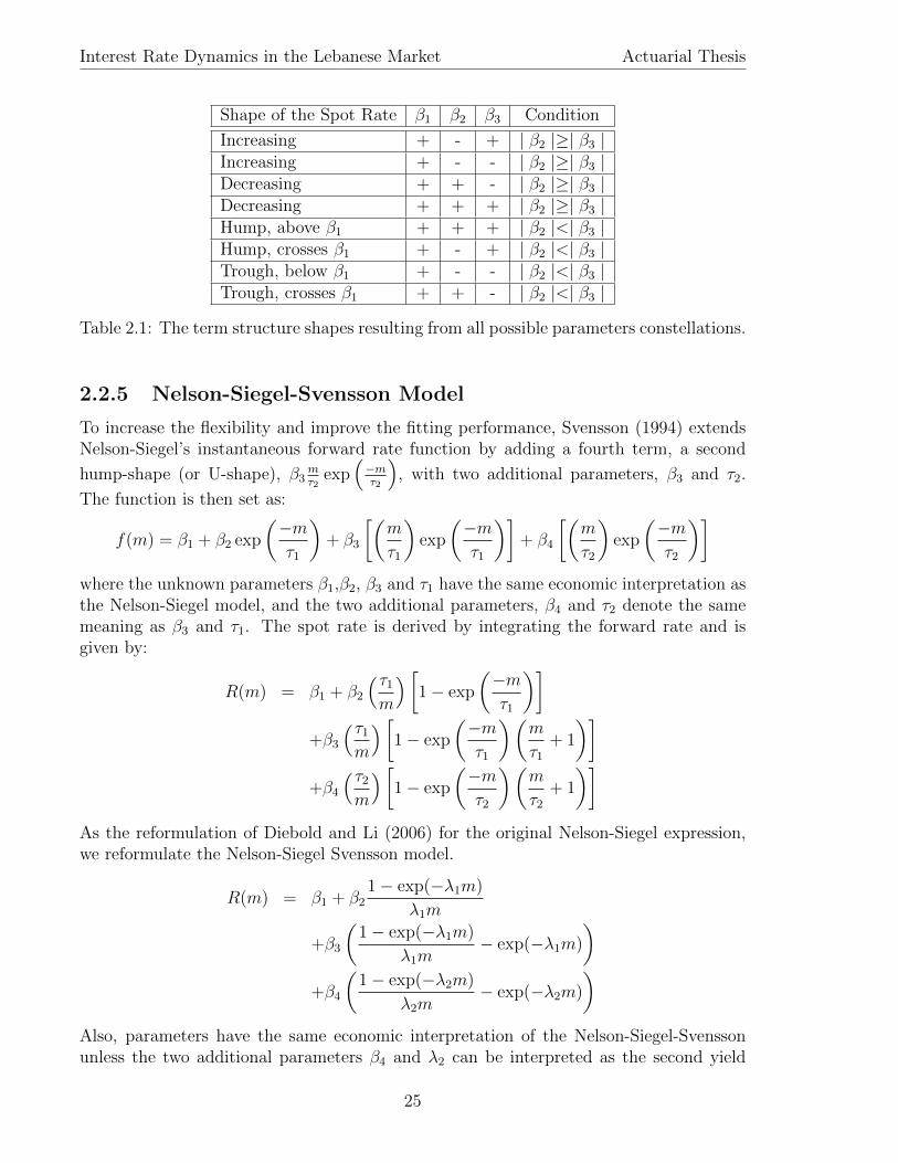
Summary Therefore, with longer time to maturity the spot rate curve approaches β1.To avoid negative interest rates β1 must be positive. If m gets small the limiting value forR(m) is (β1 +β2). Thus, also the sum (β1 +β2) is required to be positive. The parameterλ is bounded to positive values that guarantee convergence to the long term value β1. Inthe table 2.2.4, we provide a brief summary of Nelson-Siegel yield curve for all possibleparameters constellations with λ > 0.
24
Interest Rate Dynamics in the Lebanese Market Actuarial Thesis
Shape of the Spot Rate β1 β2 β3 Condition
Increasing + - + | β2 |≥| β3 |Increasing + - - | β2 |≥| β3 |Decreasing + + - | β2 |≥| β3 |Decreasing + + + | β2 |≥| β3 |Hump, above β1 + + + | β2 |<| β3 |Hump, crosses β1 + - + | β2 |<| β3 |Trough, below β1 + - - | β2 |<| β3 |Trough, crosses β1 + + - | β2 |<| β3 |
Table 2.1: The term structure shapes resulting from all possible parameters constellations.
2.2.5 Nelson-Siegel-Svensson Model
To increase the flexibility and improve the fitting performance, Svensson (1994) extendsNelson-Siegel’s instantaneous forward rate function by adding a fourth term, a second
hump-shape (or U-shape), β3mτ2
exp(−mτ2
), with two additional parameters, β3 and τ2.
The function is then set as:
f(m) = β1 + β2 exp
(−mτ1
)+ β3
[(m
τ1
)exp
(−mτ1
)]+ β4
[(m
τ2
)exp
(−mτ2
)]where the unknown parameters β1,β2, β3 and τ1 have the same economic interpretation asthe Nelson-Siegel model, and the two additional parameters, β4 and τ2 denote the samemeaning as β3 and τ1. The spot rate is derived by integrating the forward rate and isgiven by:
R(m) = β1 + β2
(τ1m
)[1− exp
(−mτ1
)]+β3
(τ1m
)[1− exp
(−mτ1
)(m
τ1+ 1
)]+β4
(τ2m
)[1− exp
(−mτ2
)(m
τ2+ 1
)]As the reformulation of Diebold and Li (2006) for the original Nelson-Siegel expression,we reformulate the Nelson-Siegel Svensson model.
R(m) = β1 + β21− exp(−λ1m)
λ1m
+β3
(1− exp(−λ1m)
λ1m− exp(−λ1m)
)+β4
(1− exp(−λ2m)
λ2m− exp(−λ2m)
)Also, parameters have the same economic interpretation of the Nelson-Siegel-Svenssonunless the two additional parameters β4 and λ2 can be interpreted as the second yield
25

Interest Rate Dynamics in the Lebanese Market Actuarial Thesis
curve shape employed to long-term yields behavior. We can’t say that Svensson modelis better than Nelson-Siegel model since he adds another shape to the curve and we willsee in the following that some central banks prefer to use Nelson-Siegel model and notSvensson model.
2.3 Zero-coupon yield curves in central banks
In this section, we provide a brief notes on approaches employed by central banks to buildthe yield curves reported to Basel Committee.National Bank of Belgium estimates the yield curve using the Nelson-Sigel-Svensson model(1994). The estimation of the parameters is based on minimizing the sum of squared bondprice errors weighted by the following function:
1 + yield to maturity
duration× price
The Bank of Canada employs the Merrill Lynch Exponential Spline model. The model isbased on a functional form for the discount function d(t), as
d(t) =9∑i=1
ak exp(−kbt)
where ak (k = 1, · · · , 9) and b are the parameters to be estimated. The estimationmethods is to minimize the sum of squared bond price errors weighted by the inverse ofthe duration of each bond.The Bank of Finland estimates the daily term structure of interest rates using the methodsdeveloped by Nelson-Siegel (1987). The estimation is based on the minimization of theyield errors.In France, the yield curve is determined by the original Nelson-Siegel function and theaugmented function as proposed by Svensson. The parameters are obtained by minimizingthe weighted sum of the square of the errors on the prices, the weights are the interestrate sensitivity factors of prices. First, the Nelson-Siegel model is being fitted to the data.Second, they introduce the two parameters that are specific to Svensson model to thefitted equation and the new parameters are estimated by the same method used to thefirst four parameters. The selection between the basic and the augmented Nelson-Siegelfunctions is based on the Fisher test (at the 5% significance level).Appendix B provides a summary table for these employed yield curve models with theirestimation methods in different central banks.
26

Interest Rate Dynamics in the Lebanese Market Actuarial Thesis
27

Chapter 3
Lebanese Yield Curve
3.1 Introduction
We showed that the model of Nelson and Siegel (1987) and its extension by Svensson(1994) are widely used by central banks as a model for the term structure of interestrates. Many academic studies show difficulties found when estimating the parameters dueto many reasons. For instance, a small change in a yield may cause a large change in theparameters due to the colinearity between the loading factors. Gilli & al. (2010) proposea new methodology for calibrating the Nelson-Siegel-Svensson model by working on thecolinearity between loadings on factors. In the following, we will build the Lebanese term-structure of interest rates using models used in different central banks and we will showthe inconvenient of these estimation methods then we will propose a new methodologyfor the calibration.
3.2 Data
At Bank Audi, or in general at Lebanese Banks, in order to calculate the economic valueof different financial products in LBP or USD currency, we build two zero-coupon yieldcurves. The data used for estimating zero coupon yield curves are divided into two parts,the first considers the Lebanese Pound Yield Curve which is built from bonds issued bythe Lebanese Government and denominated in the local currency whereas the second isthe US dollar yield curve which estimated from Eurobonds issued by the Lebanese Gov-ernment denominated in US dollar for long-term yields, and from the US treasury yieldsand the Lebanese Credit Default Swap (CDS) points for short term yields.Lebanese Government Bonds denominated in Local currency are divided into two cate-gories:
- Treasury Bills: Zero coupon bonds that mature within one year or less from theirtime of issuance.
- Treasury Notes: Bonds issued with maturities of one, three, five, seven, 10 years.
We obtain the yield of LBP bonds traded on the secondary market and we always havefor all maturities. These bonds are specialized by its illiquidity and yields might be stale
28

Interest Rate Dynamics in the Lebanese Market Actuarial Thesis
for a while before experiencing some jumps.For Eurobonds, the market is more liquid especially for newly issued bonds. We get theyields from different available maturities from the secondary market. But, sometimes,we don’t have maturing bonds in the short term, therefore we use US treasury yields towhich we add the Lebanese Credit Default Swap points as an approximation usually usedfor the first year of the yield curve.We have shown how we obtain observed rates for zero coupon bonds and coupon bondsfrom the secondary market. Therefore we apply the bootstrapping method to obtainobserved zero rates for LBP yield curve and USD yield curve. Then we apply linearinterpolation to obtain zero rates for all maturities to build the yield curve. The aim ofthe following section is to find a method more robust than the linear interpolation to buildthe yield curve from the observed zero rates obtained from the bootstrapping method.
Figures 3.1 and 3.2 represent historical zero yields for USD bonds and LBP bonds
2009
2010
2011
2012
2013 05
1015
20
0
0.02
0.04
0.06
0.08
0.1
Maturity(Years)Time(Year)
Zer
o Y
ield
s
Figure 3.1: Historical US Dollar YieldCurve (2009-2013).
20092010
20112012
2013 0 2 4 6 8 10 12
0.03
0.04
0.05
0.06
0.07
0.08
0.09
0.1
0.11
Maturity(Years)Time(Year)
Zer
o Y
ield
s
Figure 3.2: Historical Lebanese Pound YieldCurve (2009-2013).
respectively. The two surfaces show the absence of any shock on both of the yield curvesand the rates decreased slowly during these 3 years. Therefore, the long-run parameterβ1 should not have large variations during this period.
3.3 Estimation Methods
We look into the two principal models ”Nelson-Siegel” model and its extension proposedby Svensson (1994). We have to estimate four linear parameters β1, β2, β3 and β4, andtwo non-linear parameters λ1 and λ2. For n observed yields with n different maturities, wehave n equations. The simplest way to estimate the parameters is to fix λ1 and λ2, andthen estimate the β-values using ordinary least square method or maximum likelihoodmethod. But this method will guide us to unacceptable errors distribution.More generally, we can estimate the parameters of the models by minimizing the difference
29

Interest Rate Dynamics in the Lebanese Market Actuarial Thesis
between the model rates r and observed rates r thus the optimisation problem is as follows:
minimizeβ,λ
∑(r − r)2
subject to β1 > 0, β1 + β2 > 0
The two constraints let the parameters to have a clear economic interpretation, β1 > 0confirms the non-negativity of the interest rate long-run and β1 + β2 > 0 show that theovernight zero rate should be positive. However, when using this estimation method, wefound a lot of jumps in the behavior of the parameters due to the colinearity between theloadings factors:
h1(m) =1− exp(−λ1m)
λ1m
h2(m) =
(1− exp(−λ1m)
λ1m− exp(−λ1m)
)h3(m) =
(1− exp(−λ2m)
λ2m− exp(−λ2m)
)When analyzing the factor loadings, we conclude that a high correlation exists betweenthem for many values of λ1 and λ2. Figure 3.3 shows the correlation between h1(m) andh2(m), Figure 3.4 represents the surface of the function
R =
√1ρ(h1(m), h2(m))2 + ρ(h1(m), h3(m))2 + ρ(h2(m), h3(m))2
3
where ρ denotes the linear correlation.We see that correlation is -1 at λ close to zero, rapidly grows to 1 as λ grows. The
0 0.2 0.4 0.6 0.8 1−1
−0.8
−0.6
−0.4
−0.2
0
0.2
0.4
0.6
0.8
1
λ1
ρ(h 1(m
),h 2(m
))
Figure 3.3: Nelson-Sigel Loadings Correla-tion
00.2
0.40.6
0.81
0
0.5
10.4
0.5
0.6
0.7
0.8
0.9
1
λ1
λ2
R
Figure 3.4: Svensson Loadings Correlation
correlations are computed for maturities up to 10 years, so we agree that the correlationbetween the first two loading factors is negligible for a small interval of λ1. Also, for thecase of Nelson-Siegel-Svensson model, the euclidean measure of the vector of correlations
30

Interest Rate Dynamics in the Lebanese Market Actuarial Thesis
(ρ(h1, h2), ρ(h1, h3), ρ(h2, h3)) is small in value for a small range of (λ1, λ2) as observed inFigure 3.4. If we only want to obtain an approximation to the current yield curve, wedon’t need to care from the colinearity since many different parameter values give similarfits. But in this work, we are interested in giving an economic interpretation to estimatedparameters. For this issue, we will add an additional constraint to the optimization prob-lem in order to limit the correlation and obtain more robust parameters for interpretation.In other words, the new constraint adds bounds to the correlation between the two firstloading factors for Nelson-Siegel Model and to the euclidean norm of the vector of corre-lations (ρ(h1, h2), ρ(h1, h3), ρ(h2, h3)) for Nelson-Siegel-Svensson model.
Nelson Siegel Model We tend to minimize the sum of squared errors between the ob-served and the estimated yields with the given constraints:
• Non-negativity of the long run parameter limm→+∞
r(m) = β1;
• Non-negativity of the “overnight” rate r(0) = β1 + β2;
• The correlation between the two loadings factors is bounded to 0.2, to assurethe linear independence between the endogenous variables.
minimizeβ1,β2,β3,λ1
∑(r − r)2
subject to β1 > 0, β1 + β2 > 0
|ρ(h1, h2)| ≤ 0.2
Nelson Siegel Svensson Model The same constraints stated previously apply to Nel-son Siegel Svensson Model, we have added an additional constraint related to theEuclidean norm of the loadings factors correlations.The fourth constraint have been upper bounded by 0.8/
√3, since by checking Figure
3.4 we notice that R ≤ 0.8/√
3 for 1% of λ1 and λ2 values. In this way, we haveselected the 1% smallest values of R.
minimizeβ1,β2,β3,β4,λ1,λ2
∑(r − r)2
subject to β1 > 0, β1 + β2 > 0
R =
√ρ(h1, h2)2 + ρ(h1, h3)2 + ρ(h2, h3)2
3≤ 0.8√
3
We call this estimation method: “Correlation Constraint Approach”.
3.4 Application
As we mentioned above that bonds issued by the Lebanese Government are divided intotwo types zero coupon bonds and coupon bonds, we employ the bootstrapping method tocalculate the observed zero coupon yields. We use weekly zero rates for maturities 1 dayto 15 years from January 2009 until end of January 2013. For the Nelson Siegel Model,we apply the following methods:
31

Interest Rate Dynamics in the Lebanese Market Actuarial Thesis
R Package Solution: We use the functions included in the package “Yield Curve”.
Correlation Zero Method: We fix λ1 which set the correlation between loading factorsto zero then we estimate the linear parameters using ordinary least square method.
Ordinary Least Square Method: We use this method to compare it to the functionof the ”Yield Curve” package.
Correlation Constraint Approach We use the approach explained in Section 3.3.
For the Nelson-Siegel-Svensson model, we used the R package Solution and correlationconstraint approach. Before interpreting the results, we cite the required criterion for themodel validation. During doing the research, a lot of papers highlight difficulties in cali-brating these two models due to the limited observed points as we have seen for a givendate, the difference between the number of observed points on the market and the numberof parameters to be estimated is very small when applying Nelson-Siegel-Svensson model,thus the parameter are very sensitive to variations if the loading factors are linearly de-pendent.To study the residuals as a time series, we draw the histogram of available maturities forall the dates in the figures 3.5 and 3.6.
Therefore, we divide yield errors into intervals limited by the following maturities: 0,
Maturity(Years)
Fre
quen
cy
0 5 10 15
050
100
150
Figure 3.5: Histogram of Maturities forUSD Bonds
Maturity(Years)
Fre
quen
cy
0 2 4 6 8 10
050
100
150
Figure 3.6: Histogram of Maturities forLBP Bonds
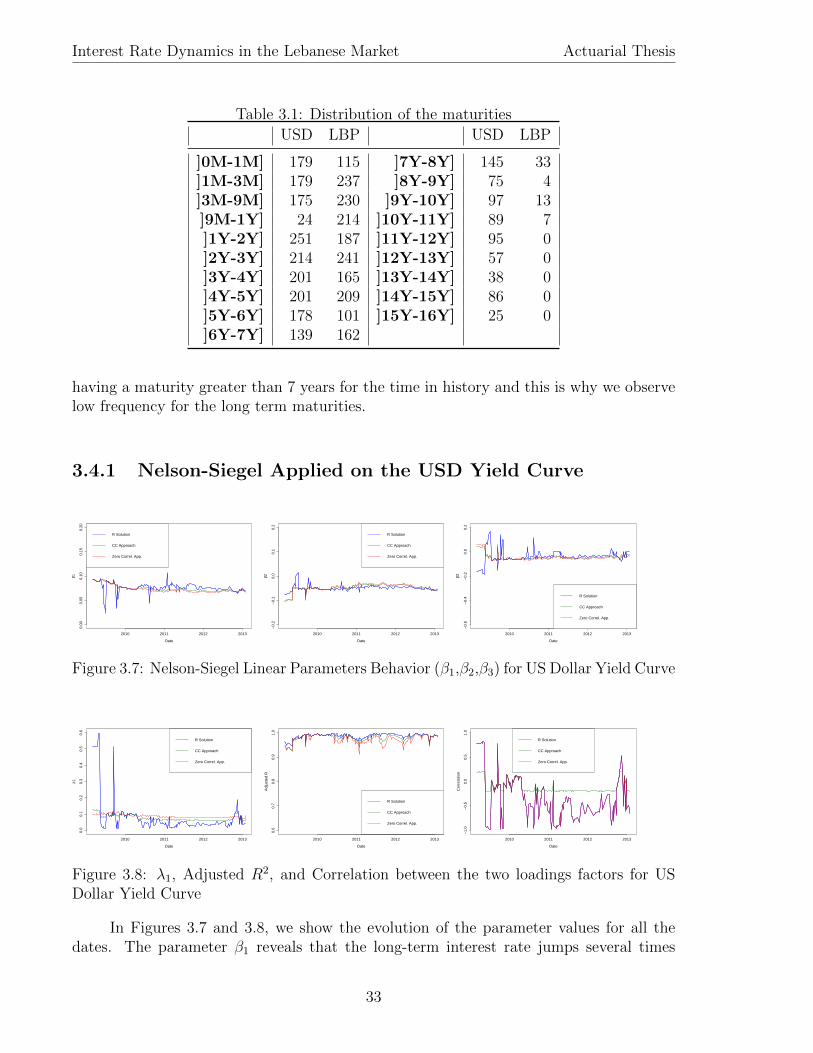
1 Month, 3 Months, 90 Months, 1 Year, 2 Years, 3 Years, 4 Years, 5 Years, 6 Years, 7Years, 8 Years, 9 Years and 10 Years. For each interval, we take yield errors as a timeseries from the start date until the last date. For a date, if there exits two errors in thesame interval we take the mean error. Then we study the distribution of theses errors tosee if the model is more robust for short term yields or long term yields.Table 3.1 represents the distribution of these maturities in figures. For the USD yields,the maturities are nearly uniformly distributed for the first eight years unless for the ma-turities around 1 year and this mismatch is due to the combination of Eurobond yieldsand US treasury yields plus Credit Default Swap, thus we will find a lot of observed yieldshaving maturities between 9 months and two years. Also, yields having maturities greaterthan 9 years are nearly uniformly distributed but with a smaller frequency. On the otherhand, for the LBP yields, the maturities are equally distributed for those less or equal to7 years, but on September 2012, the Lebanese Government started to issue LBP bonds
32
Interest Rate Dynamics in the Lebanese Market Actuarial Thesis
Table 3.1: Distribution of the maturities
USD LBP USD LBP
]0M-1M] 179 115 ]7Y-8Y] 145 33]1M-3M] 179 237 ]8Y-9Y] 75 4]3M-9M] 175 230 ]9Y-10Y] 97 13]9M-1Y] 24 214 ]10Y-11Y] 89 7]1Y-2Y] 251 187 ]11Y-12Y] 95 0]2Y-3Y] 214 241 ]12Y-13Y] 57 0]3Y-4Y] 201 165 ]13Y-14Y] 38 0]4Y-5Y] 201 209 ]14Y-15Y] 86 0]5Y-6Y] 178 101 ]15Y-16Y] 25 0]6Y-7Y] 139 162
having a maturity greater than 7 years for the time in history and this is why we observelow frequency for the long term maturities.
3.4.1 Nelson-Siegel Applied on the USD Yield Curve
2010 2011 2012 2013
0.00
0.05
0.10
0.15
0.20
Date
β1
R Solution
CC Approach
Zero Correl. App.
2010 2011 2012 2013
−0.
2−
0.1
0.0
0.1
0.2
Date
β2
R Solution
CC Approach
Zero Correl. App.
2010 2011 2012 2013
−0.
6−
0.4
−0.
20.
00.
2
Date
β3
R Solution
CC Approach
Zero Correl. App.
Figure 3.7: Nelson-Siegel Linear Parameters Behavior (β1,β2,β3) for US Dollar Yield Curve
2010 2011 2012 2013
0.0
0.1
0.2
0.3
0.4
0.5
0.6
Date
λ1
R Solution
CC Approach
Zero Correl. App.
2010 2011 2012 2013
0.6
0.7
0.8
0.9
1.0
Date
Adj
uste
d R
R Solution
CC Approach
Zero Correl. App.
2010 2011 2012 2013
−1.
0−
0.5
0.0
0.5
1.0
Date
Cor
rela
tion
R Solution
CC Approach
Zero Correl. App.
Figure 3.8: λ1, Adjusted R2, and Correlation between the two loadings factors for USDollar Yield Curve
In Figures 3.7 and 3.8, we show the evolution of the parameter values for all thedates. The parameter β1 reveals that the long-term interest rate jumps several times
33

Interest Rate Dynamics in the Lebanese Market Actuarial Thesis
when applying the R package solution. But when we refer to the historical yield curves(Figure 3.1), we see that during these two years there is no shocks neither in the short-term yields nor in the long-term yields, therefore, the estimated parameters β1 and β2should vary in a limited interval fixing the long-run of interest rates and the overnight rate.Therefore, adding the colinearity constraint has made the parameters more robust andcan be interpreted economically. The same concept applies for the third linear parameterβ3.In addition, the correlation between the two loading factors seen in Figure 3.8 showsthe three curves related to R solution package, Null correlation approach and correlationconstraint approach. In this work, the null correlation approach has fixed a λ that tendsto minimize the absolute correlation to zero; hence the zero constant red line in the figure.Comparing the two other methods, it’s obvious that the interval of the green line curvehas less boundaries then the one in blue line. Which add to the method of acceptedcorrelation more value.On the other hand the adjusted R figure in the center, calculating the fitting performanceof the three different methods using:
R2 = 1−∑n
i=1(ri − r2i )/(n− k)∑ni=1(ri − r2i )/(n− 1)
clearly shows the good fit of all three methods.
Figures 3.9 and 3.10 represent the errors in a three-dimensional plot. The first figure 3.11shows the time series of generated errors of all four categories, we mark the attentionthat on the long-run (maturity of 10 years), null correlation method fits very poorly. TheQQ-plots generated in figure 3.12 shows the normality of the errors for R package solutionand correlation constraint approach. Whereas, Figure 3.13 represents the auto-correlationfunction of the errors showing the existence of the auto-correlation in all methods thatcan be explained by the rigidity of the Nelson-Siegel function.
2009
2010
2011
2012
2013 05
1015
−0.02
−0.01
0
0.01
0.02
Maturity(Year)Time(Year)
Err
or
Figure 3.9: USD Nelson-Siegel Errors (Rsolution)
20092010
20112012
2013 05
1015
20
−0.02
−0.01
0
0.01
0.02
Maturity(Year)Time(Year)
Err
or
Figure 3.10: USD Nelson-Siegel Errors(Correlation Constraint Approach)
34

Interest Rate Dynamics in the Lebanese Market Actuarial Thesis
0 50 100 150
−0.002
0.004
R solution
0 50 100 150
−0.04
−0.01
Zero Correaltion
0 50 100 150
−0.002
0.004
Max R2
0 50 100 150
−0.004
0.004
Corr Const App
Maturity~1 Month(s)
0 20 60 100
−0.004
0.004
R solution
0 20 60 100
−0.07
−0.02
Zero Correaltion
0 20 60 100
−0.004
0.004
Max R2
0 20 60 100
−0.004
0.004
Corr Const App
Maturity~24 Month(s)
0 20 60 100
−0.0005
0.0020
R solution
0 20 60 100
−0.06
−0.01
Zero Correaltion
0 20 60 100
−0.0005
0.0020
Max R2
0 20 60 100
−0.0005
0.0020
Corr Const App
Maturity~122 Month(s)
Figure 3.11: Time Series Errors of Nelson Siegel Model Applied on USD Curve
−0.002 0.002
−0.003
0.002
R solution
−0.04 −0.02 0.00
−0.06
−0.01
Zero Correlation
−0.002 0.002
−0.003
0.003
Max R2
−0.004 0.002 0.006
−0.006
0.004
Corr Const App
Maturity~1 Month(s)
−0.004 0.000 0.004
−0.006
0.004
R solution
−0.07 −0.04 −0.01
−0.07
−0.02
Zero Correlation
−0.004 0.000 0.004
−0.006
0.004
Max R2
−0.004 0.000 0.004
−0.008
0.002
Corr Const App
Maturity~24 Month(s)
−0.0005 0.0010−0.0010
0.0020
R solution
−0.06 −0.03 0.00
−0.08
−0.04
Zero Correlation
−0.0005 0.0010
−0.0010
0.0020
Max R2
−0.0005 0.0010
−0.001
0.003
Corr Const App
Maturity~122 Month(s)
Figure 3.12: QQplot Errors of Nelson Siegel Model Applied on USD Curve
0 5 10 15 20
0.0
0.6
Lag
ACF
R solution
0 5 10 15 20
0.0
0.6
Lag
ACF
Zero Correlation
0 5 10 15 20
0.0
0.6
Lag
ACF
Max R2
0 5 10 15 20
0.0
0.6
Lag
ACF
Corr Const App
Maturity~1 Month(s)
0 5 10 15 20
−0.2
0.4
1.0
Lag
ACF
R solution
0 5 10 15 20
−0.2
0.4
1.0
Lag
ACF
Zero Correlation
0 5 10 15 20
−0.2
0.4
1.0
Lag
ACF
Max R2
0 5 10 15 20
−0.2
0.4
1.0
Lag
ACF
Corr Const App
Maturity~24 Month(s)
0 5 10 15 20
−0.2
0.4
1.0
Lag
ACF
R solution
0 5 10 15 20
−0.2
0.4
1.0
Lag
ACF
Zero Correlation
0 5 10 15 20
−0.2
0.4
1.0
Lag
ACF
Max R2
0 5 10 15 20
−0.2
0.4
1.0
Lag
ACF
Corr Const App
Maturity~122 Month(s)
Figure 3.13: Auto Correlation Errors of Nelson Siegel Model Applied on USD Curve
3.4.2 Nelson-Siegel Applied on the LBP Yield Curve
In Figures 3.14 and 3.15, the time series of estimated parameters are also plotted for allthe dates. As we have shown for the USD yield curve, the long-run parameter β1 jumpsseveral times due to small changes in yields when using the R-package solution. Accordingto the historical Lebanese Pound Yields, the estimated parameters β1 and β2 should havesmall variations since the Lebanese Bonds are illiquid and there is the absence of anyshock in their prices. Therefore, adding the colinearity constraint is essential to maintainthe variation of the parameters.
Similarly to the previous case, the correlation between the two loading factors isrepresented in Figure 3.15 the three curves related to R solution package, null correlation
35

Interest Rate Dynamics in the Lebanese Market Actuarial Thesis
2010 2011 2012 2013
0.00
0.05
0.10
0.15
0.20
Date
β1
R Solution
CC Approach
Zero Correl. App.
2010 2011 2012 2013
−0.
10−
0.05
0.00
0.05
0.10
Date
β2
R Solution
CC Approach
Zero Correl. App.
2010 2011 2012 2013
−0.
10−
0.05
0.00
0.05
0.10
Date
β3
R Solution
CC Approach
Zero Correl. App.
Figure 3.14: Nelson-Siegel Linear Parameters Behaviour (β1,β2,β3) for US Dollar YieldCurve
2010 2011 2012 2013
0.0
0.1
0.2
0.3
0.4
0.5
0.6
Date
λ1
R Solution
CC Approach
Zero Correl. App.
2010 2011 2012 2013
0.6
0.7
0.8
0.9
1.0
Date
Adj
uste
d R
R Solution
CC Approach
Zero Correl. App.
2010 2011 2012 2013
−1.
0−
0.5
0.0
0.5
1.0
Date
Cor
rela
tion
R Solution
CC Approach
Zero Correl. App.
Figure 3.15: λ1, Adjusted R2, and Correlation between the two loadings factors for USDollar Yield Curve
approach and acceptable correlation solution. The null-correlation approach is observedin the zero constant red line in the figure. Comparing the two other approaches, it’sobvious that the interval of the green line curve has less boundaries then the one in blueline as in the previous case. And again, we can say that the accepted correlation hisbetter than the other proposed methods.Turning to the adjusted R figure in the center, we observe that the fitting performanceisn’t well as we are seeking, therefore adding svensson model parameters may guide thestudy to its objective.Figures 3.16 and 3.17 plot the errors in a three-dimensional space. The first figure 3.18shows the time series of generated errors of all four categories, we mark the attention thaton the long-run(maturity of 10 years), null-correlation approach fits very poorly. The QQ-plots generated in figure 3.19 shows the normality of the errors for R package solution andaccepted correlation approach. The figure 3.20 represents the auto-correlation functionof the errors also showing the existence of the auto-correlation in all methods.
36

Interest Rate Dynamics in the Lebanese Market Actuarial Thesis
2009
2010
2011
2012
2013 02
46
810
12
−0.02
−0.01
0
0.01
0.02
Maturity(Year)Time(Year)
Err
or
Figure 3.16: LBP Nelson-Siegel Errors(R solution)
2009
2010
2011
2012
20130 2 4 6 8 10 12
−0.02
−0.01
0
0.01
0.02
Maturity(Year)Time(Year)
Err
or
Figure 3.17: LBP Nelson-Siegel Errors(Acceptable Correlation solution)
0 40 80
0.000
0.006
R solution
0 40 80
−0.05
−0.01
Zero Correaltion
0 40 80
0.000
0.006
Max R2
0 40 80
0.001
0.006
Corr Const App
Maturity~1 Month(s)
0 50 100 150
−0.002
0.006
R solution
0 50 100 150
−0.08
−0.02
Zero Correaltion
0 50 100 150
−0.002
0.006
Max R2
0 50 100 150
−0.002
0.006
Corr Const App
Maturity~24 Month(s)
5 10 15 20
−0.0045
R solution
5 10 15 20
−0.08
−0.02
Zero Correaltion
5 10 15 20−0.0046
−0.0032
Max R2
5 10 15 20−0.0065
−0.0050
Corr Const App
Maturity~122 Month(s)
Figure 3.18: Time Series Errors of Nelson Siegel Model Applied on LBP Curve
0.000 0.004
−0.002
0.008
R solution
−0.05 −0.03 −0.01
−0.05
−0.02
Zero Correlation
0.000 0.004
−0.002
0.008
Max R2
0.001 0.004−0.002
0.006
Corr Const App
Maturity~1 Month(s)
−0.002 0.002 0.006
−0.005
R solution
−0.08 −0.04 0.00
−0.10
−0.04
Zero Correlation
−0.002 0.002 0.006
−0.005
0.010
Max R2
−0.002 0.002 0.006
−0.005
Corr Const App
Maturity~24 Month(s)
−0.0045 −0.0035
−0.0050
R solution
−0.08 −0.04
−0.14
−0.04
Zero Correlation
−0.0046 −0.0038−0.0050
Max R2
−0.0065 −0.0055
−0.007
−0.004
Corr Const App
Maturity~122 Month(s)
Figure 3.19: QQplot Errors of Nelson Siegel Model Applied on LBP Curve
0 5 10 15 20
−0.2
0.6
Lag
ACF
R solution
0 5 10 15 20
−0.2
0.4
1.0
Lag
ACF
Zero Correlation
0 5 10 15 20
−0.2
0.6
Lag
ACF
Max R2
0 5 10 15 20
−0.2
0.6
Lag
ACF
Corr Const App
Maturity~1 Month(s)
0 5 10 15 20
0.0
0.6
Lag
ACF
R solution
0 5 10 15 20
0.0
0.6
Lag
ACF
Zero Correlation
0 5 10 15 20
0.0
0.6
Lag
ACF
Max R2
0 5 10 15 20
0.0
0.6
Lag
ACF
Corr Const App
Maturity~24 Month(s)
0 2 4 6 8 12
−0.4
0.4
Lag
ACF
R solution
0 2 4 6 8 12
−0.4
0.4
Lag
ACF
Zero Correlation
0 2 4 6 8 12
−0.4
0.4
Lag
ACF
Max R2
0 2 4 6 8 12
−0.4
0.4
Lag
ACF
Corr Const App
Maturity~122 Month(s)
Figure 3.20: Auto Correlation Errors of Nelson Siegel Model Applied on LBP Curve
3.4.3 Nelson-Siegel-Svensson Applied on the USD Yield Curve
The behaviors of the parameter values are represented in Figures 3.21 and 3.22. We haveshown that in the Nelson-Siegel model there exists several jumps in the long-run parameter
37

Interest Rate Dynamics in the Lebanese Market Actuarial Thesis
due to the collinearity of the two loading factors; whereas in the Nelson-Siegel-Svensson,we have three factor loading factors that the last two are very similar. Hence, applying Rsolution will guide us to observe lot of jumps in the time series of β1 due to small changesin yields. We reject the absence of these jumps by referring to the historical LebanesePound Yields which shows small changes in yields and by the collinearity hypothesis forthe ordinary least square method. Nevertheless, we observe a large set of dates the long-run is negative or greater than 0.12 when neglecting the correlation criteria. The sameanalysis is done for β2 to maintain the long-run of interest rates and the overnight rate.Thus, in order to obtain more robust parameters we should add the collinearity constraint.
2010 2011 2012 2013
0.0
0.1
0.2
0.3
Date
β1
R Solution
CC Approach
2010 2011 2012 2013
−0.
3−
0.2
−0.
10.
00.
10.
20.
3
Date
β2
R Solution
CC Approach
2010 2011 2012 2013
−0.
6−
0.4
−0.
20.
00.
2
Date
β3
R Solution
CC Approach
Figure 3.21: Nelson-Siegel-Svensson Linear Parameters Behaviour (β1,β2,β3) for US DollarYield Curve
2010 2011 2012 2013
−0.
8−
0.6
−0.
4−
0.2
0.0
0.2
Date
β4
R Solution
CC Approach
2010 2011 2012 2013
0.0
0.5
1.0
1.5
2.0
Date
λ1
R Solution
CC Approach
2010 2011 2012 2013
0.6
0.7
0.8
0.9
1.0
Date
Adj
uste
d R
R Solution
CC Approach
Figure 3.22: β4, λ1, Adjusted R2 for US yield curve
Concerning the fitting performance, we observe that the adjusted R2 is higher thanthe nelson-siegel model for the both approaches. Therefore, for the Lebanese GovernmentEurobonds, it is better to employ the Svensson model. Figures 3.23 and 3.24 show theerrors in a three-dimensional plot where errors seems to be small as a consequence fromthe high adjusted R2. Figures 3.25, 3.26 and 3.27 show the time series of generatederrors of the two fitting models, we mark the attention that on the mid and long-runmaturities, the two methods have residuals almost normally distributed. But, for theshort-term yields, the residuals of the acceptable correlation approach are far from thenormal distribution and it can be explained by the mismatch between the yields used forthe short-term and long-term bonds. This mismatch will be discussed in details in theconclusion of this section. The mismatch illustrated by Svensson adds to him a positivevalue to be admitted. Also, an auto-correlation exists in all residuals deduced from thetwo fitting approaches.
38

Interest Rate Dynamics in the Lebanese Market Actuarial Thesis
2009
2010
2011
2012
2013 0 2 4 6 8 10 12 14 16
−0.02
−0.01
0
0.01
0.02
Maturity(Year)Time(Year)
Err
or
Figure 3.23: LBP Nelson-Siegel-Svensson Errors (R solution)
20092010
20112012
2013 05
1015
20−0.02
−0.01
0
0.01
0.02
Maturity(Year)Time(Year)
Err
or
Figure 3.24: LBP Nelson-Siegel-Svensson Errors (Acceptable Correla-tion solution)
0 100−1e−03
R solution
0 100
−0.006
Corr Const AppMaturity~1 Month(s)
0 60
−0.002
R solution
0 60
−0.004
Corr Const AppMaturity~24 Month(s)
0 60
−0.001
R solution
0 60−0.0005
Corr Const AppMaturity~122 Month(s)
Figure 3.25: Time Series Errors of Nelson-Siegel-Svensson Model Applied on LBP Curve
−1e−03 1e−03
−0.001
0.002
R solution
−0.006 0.000
−0.006
0.002
Corr Const AppMaturity~1 Month(s)
−0.002 0.004−0.006
0.002
R solution
−0.004 0.002
−0.006
0.002
Corr Const AppMaturity~24 Month(s)
−0.001 0.002
−0.002
0.002
R solution
−0.0005 0.0015
−0.0010
0.0020
Corr Const AppMaturity~122 Month(s)
Figure 3.26: QQplot Errors of Nelson-Siegel-Svensson Model Applied on LBP Curve
0 10
−0.2
0.8
Lag
ACF
R solution
0 10
0.0
1.0
Lag
ACF
Corr Const AppMaturity~1 Month(s)
0 10
−0.2
0.8
Lag
ACF
R solution
0 10
−0.2
0.8
Lag
ACF
Corr Const AppMaturity~24 Month(s)
0 10
−0.2
0.8
Lag
ACF
R solution
0 10
−0.2
0.8
Lag
ACF
Corr Const AppMaturity~122 Month(s)
Figure 3.27: Auto Correlation Errors of Nelson-Siegel-Svensson Model Applied on LBPCurve
3.4.4 Nelson-Siegel-Svensson Applied on the LBP Yield Curve
In Figures 3.28 and 3.29, we draw the evolution of the parameter values also for all thedates. The same analysis done on the USD yield curve Nelson-Siegel-Svensson method isapplied for this case. β1 and β1 + β2 must have small variations for all the dates.
The same interpretation for the adjusted R2 which is higher in this case than thecase of nelson-siegel model. Figures 3.30 and 3.31 show the small absolute value of errorsand the good fit done by the svensson model. Moreover, the analysis of residuals can be
39

Interest Rate Dynamics in the Lebanese Market Actuarial Thesis
2010 2011 2012 2013
0.0
0.1
0.2
0.3
Date
β1
R Solution
CC Approach
2010 2011 2012 2013
−0.
3−
0.2
−0.
10.
00.
10.
20.
3
Date
β2
R Solution
CC Approach
2010 2011 2012 2013
−0.
6−
0.4
−0.
20.
00.
2
Date
β3
R Solution
CC Approach
Figure 3.28: Nelson-Siegel-Svensson Linear Parameters Behaviour (β1,β2,β3) for LBPYield Curve
2010 2011 2012 2013
−0.
8−
0.6
−0.
4−
0.2
0.0
0.2
Date
β4
R Solution
CC Approach
2010 2011 2012 2013
0.0
0.5
1.0
1.5
2.0
Date
λ1
R Solution
CC Approach
2010 2011 2012 2013
0.6
0.7
0.8
0.9
1.0
Date
Adj
uste
d R
R Solution
CC Approach
Figure 3.29: β4, λ1, Adjusted R2 for LBP yield curve
done by interpreting results outlined in the figures 3.32, 3.33 and 3.34. In fact, residualsare normally distributed for the two methods which also adds value to Svensson modelbut the autocorrelation problem isn’t resolved yet.
2009
2010
2011
2012
2013 02
46
810
12
−0.02
−0.01
0
0.01
0.02
Maturity(Year)Time(Year)
Err
or
Figure 3.30: LBP Nelson-Siegel-Svensson Errors (R solution)
2009
2010
2011
2012
2013 0 2 4 6 8 10 12
−0.02
−0.01
0
0.01
0.02
Maturity(Year)Time(Year)
Err
or
Figure 3.31: LBP Nelson-Siegel-Svensson Errors (Acceptable Correla-tion solution)
0 60−0.0005
R solution
0 60−0.003
Corr Const AppMaturity~1 Month(s)
0 100−0.0005
R solution
0 100
−0.001
Corr Const AppMaturity~24 Month(s)
5 15
−8e−04
R solution
5 15
−0.0020
Corr Const AppMaturity~122 Month(s)
Figure 3.32: Time Series Errors of Nelson-Siegel-Svensson Model Applied on LBP Curve
40
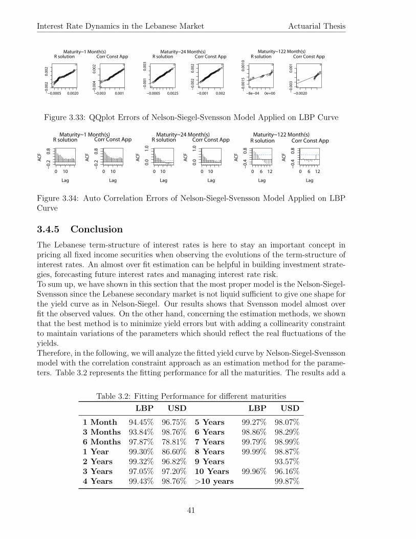
Interest Rate Dynamics in the Lebanese Market Actuarial Thesis
−0.0005 0.0020−0.002
0.002
R solution
−0.003 0.001−0.004
0.002
Corr Const AppMaturity~1 Month(s)
−0.0005 0.0025
−0.001
0.003
R solution
−0.001 0.002
−0.002
0.002
Corr Const AppMaturity~24 Month(s)
−8e−04 0e+00
−0.0015
0.0010
R solution
−0.0020
−0.003
0.001
Corr Const AppMaturity~122 Month(s)
Figure 3.33: QQplot Errors of Nelson-Siegel-Svensson Model Applied on LBP Curve
0 10
−0.2
0.8
Lag
ACF
R solution
0 10
−0.2
0.8
Lag
ACF
Corr Const AppMaturity~1 Month(s)
0 10
0.0
1.0
Lag
ACF
R solution
0 10
0.0
1.0
Lag
ACF
Corr Const AppMaturity~24 Month(s)
0 6 12
−0.4
0.8
Lag
ACF
R solution
0 6 12
−0.4
0.8
Lag
ACF
Corr Const AppMaturity~122 Month(s)
Figure 3.34: Auto Correlation Errors of Nelson-Siegel-Svensson Model Applied on LBPCurve
3.4.5 Conclusion
The Lebanese term-structure of interest rates is here to stay an important concept inpricing all fixed income securities when observing the evolutions of the term-structure ofinterest rates. An almost over fit estimation can be helpful in building investment strate-gies, forecasting future interest rates and managing interest rate risk.To sum up, we have shown in this section that the most proper model is the Nelson-Siegel-Svensson since the Lebanese secondary market is not liquid sufficient to give one shape forthe yield curve as in Nelson-Siegel. Our results shows that Svensson model almost overfit the observed values. On the other hand, concerning the estimation methods, we shownthat the best method is to minimize yield errors but with adding a collinearity constraintto maintain variations of the parameters which should reflect the real fluctuations of theyields.Therefore, in the following, we will analyze the fitted yield curve by Nelson-Siegel-Svenssonmodel with the correlation constraint approach as an estimation method for the parame-ters. Table 3.2 represents the fitting performance for all the maturities. The results add a
Table 3.2: Fitting Performance for different maturities
LBP USD LBP USD
1 Month 94.45% 96.75% 5 Years 99.27% 98.07%3 Months 93.84% 98.76% 6 Years 98.86% 98.29%6 Months 97.87% 78.81% 7 Years 99.79% 98.99%1 Year 99.30% 86.60% 8 Years 99.99% 98.87%2 Years 99.32% 96.82% 9 Years 93.57%3 Years 97.05% 97.20% 10 Years 99.96% 96.16%4 Years 99.43% 98.76% >10 years 99.87%
41

Interest Rate Dynamics in the Lebanese Market Actuarial Thesis
value to Svensson model to be employed as an estimator for the historical yields in orderto study the historical evolution of yields with fixed maturities not greater than 10 years.For the LBP yield curve, as we have mentioned the absence for the bonds having ma-turities less than seven years for the period before september 2012 when the Lebanesegovernment issued bonds having maturities greater than 7 years and denominated inLBP for the time in history, we would like to do further studies on the sensitivity of theyield curve. For this matter, we estimated the parameters basing on bonds maturing lessthan 7 years then we predict zero yields having maturity greater than 7 years. Figure3.35 shows the impact of the issuing new bonds on the adjusted R2 where the blue linedenotes the old fitting performance indicator and the red line the new one. Therefore, asusually, extending the yield curve is not a good indicator for the yields of bonds couldbe issued with a maturity larger than the biggest available bond maturity in the market.Of course, issuing new bonds with new maturities will guide to a movement in the yieldcurve because this effect is due to a change in the monetary strategy of the government.We didn’t do the same for the USD yield curve since short-term yields, US treasury plusCDS, hold 50% of observed yields possessing maturities less than 7 years. So we can’t dothe same study due to liquidity mismatch. But, we have eliminated all the yields havingmaturities less or equal to one year and we keep yields observed on the secondary Lebanesemarket and we show the fitting performance without adding the calculated yields to themodel. Figure 3.36 shows the almost over fit the mid and long term yields.
Nov Jan
0.6
0.7
0.8
0.9
1.0
Date
Adj
uste
d R
2
Figure 3.35: Black: Adjusted R2 of the fit-ted LBP yield curve; Red: Adjusted R2 ofthe fitted LBP yield curve using yields lessthan 7 years
2010 2011 2012 2013
0.5
0.6
0.7
0.8
0.9
1.0
Date
Adj
uste
d R
2
Figure 3.36: Adjusted R2 of the USD yieldcurve fitted only on observed Eurobondsyields on the secondary Lebanese Market
3.5 Lebanese Yield Curves Movements
To adjust the movement of the Lebanese Yield Curve, we apply the principal componentanalysis as we have done for the Euro France Eurobond Yields in Section 2.3.For the USD yield curve, we build the historical yield curves using Nelson-Siegel-Svensson
42

Interest Rate Dynamics in the Lebanese Market Actuarial Thesis
model with correlation constraint approach. Then we calculate the first difference yieldsand we apply the principal component analysis. The results are outlined in the table C.1.A brief summary of the USD yield curve is outlined hereafter:
Movement 1: Twist or change in the slope of the yield curve (Probability=57.6%)
Movement 2: Parallel Shift (Probability=37.2%)
Movement 3: Bowing in the yield curve (Probability=3.6%)
Generally, first loading factors should be similar to the first loading factors of Nelson-SiegelSvensson model. But in this case, the first loading factor with 57.6% as a proportion ofthe variance isn’t a parallel shifting which has the same behavior as of the first loadingfactor. This can be explained by the mismatch between the liquidity of the LebaneseEurobonds and the US treasury bonds since this yield curve is built from these twovariables. Moreover, the US treasury yield are more volatile than Lebanese Eurobondsand can behave differently due to many reasons, hence this mismatch can be observed instudying yield curve movements when applying principal component analysis. To resolvethis problem, in Figure 3.37, we eliminated the first component factor from the curve inorder to compare the next four component factors to the four Svensson loading factors.Curves confirm both loading factors and component factors having the same behaviorafter eliminating the first one. Nevertheless, we eliminated the yields having maturitiesless than 1 year which are extracted from the US treasury yields and the credit defaultspread, we fit the svensson yield curve to the available observed yields on the LebaneseMarket then we estimate short term yields by extending the estimated curve to the shortterm yields. And we apply the principal component analysis and its results are in thetable C.3 which show the absence of a parallel shifting in the first component factor andwe can say that adding US treasury plus CDS isn’t the best solution to construct theterm-structure of USD zero yields but is better than eliminating them and extending thecurve for the short term yields.
-0.8
-0.6
-0.4
-0.2
0
0.2
0.4
0.6
0 20 40 60 80 100 120 140PC2
PC3
PC4
PC5
-0.15
-0.1
-0.05
0
0.05
0.1
0.15
0 20 40 60 80 100 120 140
Factor 1
Factor 2
Factor 3
Factor 4
Figure 3.37: Component Factors (USD Yield Curve) compared to Nelson-Siegel-Svenssonloading factors
43

Interest Rate Dynamics in the Lebanese Market Actuarial Thesis
Turning to the Lebanese Yield Curve, the output obtained from the principal com-ponent analysis is in the table C.2 and hereafter outlines a brief summary of the results:
Movement 1: Parallel Shift (Probability=88.5%)
Movement 2: Twist or change in the slope of the yield curve (Probability=7.6%)
Movement 3: Bowing in the yield curve (Probability=1.7%)
The first three principal components explain almost all of the variance of interest ratechanges. The first factor accounts for 88.5% of the total variance, while the second andthird factors accounts for 7.6% and 1.3%, respectively. In sum the first three principalcomponents explain 98% percent of the variability of the data, which indicate that thesefactors are sufficient for describing the changes in the term structures. We represent themin the figure 3.38 with a comparison to the loading factors of Nelson-Siegel-Svenssonmodel.The first component basically represents a parallel change in LBP yield curve, and this
-1
-0.8
-0.6
-0.4
-0.2
0
0.2
0.4
0.6
0 20 40 60 80 100 120 140
PC1
PC2
PC3
PC4
-0.2
-0.15
-0.1
-0.05
0
0.05
0.1
0.15
0 20 40 60 80 100 120 140Factor 1
Factor 2
Factor 3
Factor 4
Figure 3.38: Component Factors (LBP Yield Curve) compared to Nelson-Siegel-Svenssonloading factors
is why we usually call β1 as the level or the height factor. The second principal representsa change in the steepness, is named the slope factor as β2. The third principal componentis called the curvature curve the same interpretation of β3, as it basically affects thecurvature of the Yield curve by inducing a butterfly shift.
44

Interest Rate Dynamics in the Lebanese Market Actuarial Thesis
3.6 Economical Interpretation
2010 2011 2012 2013
0.0
80
.09
0.1
00
.11
0.1
20
.13
0.1
40
.15
Time
β1
Zone 1
m= 0.1235
s= 0.0063
Zone 2
m= 0.0923
s= 0.0033
Zone 3
m= 0.094
s= 0.0067
Zone 4
m= 0.0786
s= 9e−04
Zone 5
m= 0.0981
s= 0.0037
2010 2011 2012 2013
−0
.10
−0
.08
−0
.06
−0
.04
−0
.02
Time
β2
Zone 1
m= −0.0876
s= 0.0052
Zone 2
m= −0.0636
s= 0.0032
Zone 3
m= −0.0622
s= 0.0064
Zone 4
m= −0.055
s= 0.0022
Zone 5
m= −0.0688
s= 0.0025
2010 2011 2012 2013
−0
.2−
0.1
0.0
0.1
0.2
0.3
0.4
0.5
Time
β3
Zone 1
m= 0.0754
s= 0.0855
Zone 2
m= −0.0191
s= 0.09
Zone 3
m= 0.023
s= 0.0151
Zone 4
m= −0.0377
s= 0.0112
Zone 5
m= 0.0407
s= 0.0392
2010 2011 2012 2013
−0
.2−
0.1
0.0
0.1
0.2
0.3
0.4
0.5
Time
β4
Zone 1
m= −0.1435
s= 0.1004
Zone 2
m= 0.0073
s= 0.1156
Zone 3
m= −0.1038
s= 0.0256
Zone 4
m= 0.0643
s= 0.0068
Zone 5
m= −0.0921
s= 0.0601
2010 2011 2012 2013
0.1
0.2
0.3
0.4
0.5
0.6
Time
λ1
Zone 1
m= 0.2001
s= 0.033
Zone 2
m= 0.1695
s= 0.0563
Zone 3
m= 0.1717
s= 0.027
Zone 4
m= 0.1215
s= 0.0099
Zone 5
m= 0.1274
s= 0.0169
2010 2011 2012 2013
0.1
0.2
0.3
0.4
0.5
Time
λ2
Zone 1
m= 0.117
s= 0.042
Zone 2
m= 0.1873
s= 0.0728
Zone 3
m= 0.0691
s= 0.017
Zone 4
m= 0.3314
s= 0.0276
Zone 5
m= 0.0714
s= 0.0467
β1β1β1
β3β3β3
λ1λ1s= 0.027
β2β2β2
β4β4β4β4β4
λ2
Figure 3.39: Estimated Svensson Parameters using Constraint Correlation Approach di-vided into 5 regimes.
0 2 4 6 8 10
0.04
0.06
0.08
0.10
Maturity(Years)
Yie
ld
Jun 2009(I)
Feb 2010(II)
Dec 2010(III)
May 2012(IV)
Jan 2013(V)
Figure 3.40: Lebanese Pound Fitted Yield Curve on 5 dates of different regimes.
45

Interest Rate Dynamics in the Lebanese Market Actuarial Thesis
Both methods, Ordinary Least Squared errors used by R packages and “Correlationconstraint approach”, give a well fit of observable yields. However, a good approximationto yield curve should not only fit well in sample but also forecast well out-of sample (c.f.Diebold and Li 2006). For this issue, we studied the stationarity of Svensson parametersobtained from the correlation constraint approach by using Augmented Dickey Fuller testwhich shows that they are integrated of order 0 or 1, moreover Johansen Cointegrationtest confirm the absence of any cointegration relationship between parameters integratedof order 1. Therefore, these time series can be forecasted using autoregressive integratedmoving average models. But when observing time series, we conclude that a regimeswitching model is better to be employed in this case; moreover the evolution of the pa-rameters can be economically interpreted. It is also known that the Lebanese economydepends largely on the political situation since it is considered as a touristic country forpeople coming from the Arabian Gulf.
Unfortunately, the historical data are not sufficient to build econometric models predic-tion, so we give a brief economical interpretation for the evolution of parameters. Figure3.6 shows the existence of five different regimes. The first phase is between January 2009and September 2010, we observe high yields for all maturities during this period becauseLebanon was emerging from four years of violence and political problems. It started bythe assassination of the former prime minister Rafik Harriri and the cedar revolution caus-ing the withdrawal of Syrian troops from Lebanon in 2005. The political assassinationsdidn’t end in 2005; a series of bombs attacks rocked Lebanon during the next two years.On 12th of July 2006, Israel declared the war on Lebanon. This conflict have killed 1200Lebanese people and severely damaged Lebanese civil infrastructure. Nevertheless, in2007, there was a conflict between Fatah al-Islam, an Islamist militant organization, andthe Lebanese Army; and several terrorist bombings took place in and around Lebanon’scapital, Beirut. The war ended in September 2007. In 2008, after a conflict with Futuremovement militiamen loyal to the government, Hezbollah took control of all the capital.It ended with a deal between Lebanese leaders on May 21, 2008 to terminate the 18 monthpolitical feud that exploded into fighting and nearly drove the country to a new civil war.
In the second and third phase, the yield curve affected a negative parallel shifting whichshows amelioration in the Lebanese economical situation and we observe the volatilityis higher in the second phase which can be called as an transformation phase from firstregime to the third. In fact, after the elections of 2009, the Lebanese government wasconstituted of all Lebanese political movements. Moreover, in 2008, there was the globalfinancial crisis which guide to a rise of liquidity in the Lebanese banking system and ofthe reserves at the central bank. Thus, banks had excess liquidity with restricted invest-ments opportunities incurred unnecessary higher costs of funds which led to a decline ininterest rates independently of international markets. The Lebanese economy continuedto demonstrate remarkable resilience to the global financial crisis, as signs of improvementin domestic conditions gave a boost to real economy activity with raising its real GDPgrowth estimated to 7.0% for 2009. Although, we mention the growth of passengers atthe airport (26.3%) and the evolution of real estate prices which increased 200% during2 years.
46

Interest Rate Dynamics in the Lebanese Market Actuarial Thesis
On the 15th of March 2011, a popular uprising started against the Baathist Regime ofBachar El Assad in Syria. This uprising was peaceful at the beginning, but it was slowlytransformed into a military confrontation between the newly formed Free Syrian Army(FSA) and the pro Assad (pro governmental) Syrian Arab Army (SAA) in the first quarterof 2012. Taking into consideration that Lebanon share with Syria a common border thatextends from the north east to the south west of the country, making Syria the obligatorypassage from Lebanon to the Arab Gulf countries, this conflict affected negatively theLebanese economical situation: the Arab tourists were able to reach Lebanon throughland, and the commercial transitions between Lebanon and the rest of middle-east re-gion was slowed down. Moreover, fighting from the Syrian civil war has spilled over intoLebanon. Fighting has mainly occurred between Lebanese opponents and supporters ofthe Syrian government, the spillover conflict has resulted in violent unrest and kidnap-pings of foreign citizens across Lebanon. Islamists across northern Lebanon have arrangedsit-ins and blocked roads to protest the arrest of a Lebanese Islamist linked to the Syr-ian uprising. The conflict escalated from previous sectarian clashes between pro-Syriangovernment Alawites and anti-Syrian government Sunni militants in Tripoli in June 2011and February 2012. Sit-ins were also held in south Lebanon by anti-Hezbollah Salafists,which heightened tensions further. It evolved into a conflict between the anti-SyrianMarch 14 Alliance and the pro-Syrian March 8 Alliance. The Saudi backed March 14alliance supports the Syrian rebels, whereas the Iranian backed March 8 alliance supportsthe Syrian government. This caused a slow down in the tourism of Lebanon. Addingto this, Lebanese banks’ operations in neighboring Syria have lost a combined of $400million during the first 20-month-old conflict there1. This turmoil can be observed in thetransformation from phase 3 to phase 4 when mid term yields shifted up slowly.
At the beginning of the fourth quarter of 2012, the finance ministry issued 10 year trea-sury bills in Lebanese denominated currency with 8.25% interest for the first time in thehistory of Lebanon. The subscription in the 10 year bonds was just one of series of stepstaken by the Central Bank to raise the interest to more than 8 percent. This guided tomost Lebanese banks to refrain from subscribing to the short and medium-term T-bills be-cause the yields on them were too small and therefore not very appealing to investors andlenders. This description is explained in the fifth phase after issuing the new governmentbonds.
3.7 Conclusion
In the model of the term structure applied in this chapter, we arrived to build the LBPYield Curve and US Yield Curve based on bonds issued by the Lebanese Government. Forthe USD yield curve, the term structure is built from two different types of Bonds, for theshort-term we used US treasury bonds plus Lebanese Credit Default spread. This mis-match was illustrated in the principal component analysis when the most probable yieldcurve movement was not a parallel shifting. To resolve this problem, we tried to estimate
1Source: Reuters(21 November 2012)
47

Interest Rate Dynamics in the Lebanese Market Actuarial Thesis
the yield curve basing only on observed Eurobonds yields issued by the Lebanese Govern-ment on the secondary market but the results wasn’t as we was aiming, therefore addingUS treasury yields for the short-term is a temporary solution and shouldn’t be permanent.
For the Lebanese Yield Curve, we showed that “Correlation Constraint Approach” isa good solution for in-sample and out-of-sample data. Augmented-Dickey Fuller test con-firm that obtained parameters are integrated of order 0 or 1, however when observing thetime series we conclude that a regime switching may exist in parameters due to exogenousfactors. We interpreted the evolution of the parameters by a political-economical analysis.Nevertheless, due to the insufficiently of the observed yields, we can’t apply time seriesmodels for the forecasting. An alternate solution is to take an economic expert opinion forthe upcoming economical situation to predict the future possible movement of the yieldcurve. Today, the upcoming situation can’t be expected before the formation of the newLebanese government and the elections of a new parliament without waiting for the endof the current Syrian Civil war.
48

Interest Rate Dynamics in the Lebanese Market Actuarial Thesis
49

Chapter 4
Vector Autoregression and ErrorCorrection Model
4.1 Introduction
Multivariate time series methods are widely used by a lot of financial analysts. Theeconometricians have focused on the time series analysis which could help us in answeringeconomic and financial questions. In this chapter, we provide the theoretical backgroundof two models widely used in studying linear dependencies between variables: VectorAutoregression Model (VAR) and Vector Error Correction Model (VECM). First sectionoutlines the statistical tools used to verified the required hypothesis for applying one ofthe models, whereas in the second section we provide a brief description of the two models.
4.2 Statistical Background
4.2.1 Stationarity
A stationary variable is a stochastic process that doesn’t change when shifted in time orspace. The parameters such as the mean and the variance, if it exists, also don’t changeover time or position.
Unit Root Process
A linear stochastic process has a unit root if 1 is a root of the process’s characteristicequation. In other words, we consider a discrete time stochastic process yt and supposethat it can be written as an auto-regressive process of order p:
yt = a1yt−1 + a2yt−2 + + apyt−p + εt
where εt is a white noise process. If m = 1 is a root of the characteristic equation,
mp − a1mp−1 − a2mp−2 − · · · − ap = 0,
then the stochastic process has a unit root. The properties and characteristics of unit-rootprocesses are:
50

Interest Rate Dynamics in the Lebanese Market Actuarial Thesis
• Shocks to a unit root process have permanent effects which do not decay as theywould if the process were stationary.
• A unit root process has a variance that depends on t, and diverges to infinity1.
• If it is known that a series has a unit root, the series can be differenced to render itstationary.
Stationary Process
A stochastic process is stationary if their first and second moments are time invariant. Inother words, a stochastic process xt is stationary if:
• E(Xt) = µ, ∀t.
• cov(Xt, Xt+j) = γj, ∀t, j
We have said that the variance of a unit process depends on time t therefore a unit rootprocess is non-stationary2.
Unit Root Tests
In order to test the stationarity or non-stationarity of a time series, we use the unitroot theory which has been developed by Dickey and Fuller. In our work, we selectthe Augmented Dickey-Fuller test more for convenience than any other reason. Theaugmented Dickey-Fuller test constructs a model with higher order lag and tests thesignificance of the parameter estimates using non-standard t-test. The model used forthis test is:
∆xt = α1xt−1 + 1∆xt−1 + β2∆xt−2 + · · ·+ p−1∆xt−p+1 + εt
where the t-test checks significance of the α1 term3.
Order of Integration
A time series is integrated of order 0 if the series is stationary and we note Xt ∼ I(0). Atime series is integrated of order P if:
(1− L)PXt ∼ I(0)
Where L is the lag operator and we note Xt ∼ I(P ). In other words, a series is said tobe integrated of order 1 if although it is itself non-stationary, the changes in this seriesform a stationary. It is said to be integrated of order 2 if, although the changes are non-stationary, the changes in changes form a stationary series. Generally, if the series mustbe differenced k times to achieve stationary, then the series is integrated of order k.
1Proof: Appendix D.12Proof: Appendix D.23Proof: Appendix D.3
51
Interest Rate Dynamics in the Lebanese Market Actuarial Thesis
4.2.2 Granger Causality Test
One of the key questions that can be addressed with vector autoregressions is how usefulsome variables are for forecasting others. This section discusses Granger causality testwhich is an econometric tool to study the causality. The idea of Granger causality is apretty simple one:”A variable X Granger-causes Y if Y can be better predicted using the histories of bothX and Y than it can use the history of Y alone.”To implement this test, we assume a particular autoregressive lag length p and estimatedby OLS method:
xt = c1 + a1xt−1 + a2xt−2 + · · ·+ apxt−p + b1yt−1 + b2yt−2 + · · ·+ bpyt−p + ut
We then conduct an F test of the null hypothesis:
H0 : b1 = b2 = = bp = 0
We calculate the sum of squared residuals and we obtain:
RSS1 =T∑t=1
u2t
And we estimate the coefficients of the univariate regression for xt:
xt = c1 + c1xt−1 + c2xt−2 + · · ·+ cpxt−p + εt
Then we calculate the sum squared residuals of the univariate model:
RSS0 =T∑t=1
ε2t
The objective is to compare RSS1 with RSS0. For this purpose, we calculate the followingratio:
S1 =
RSS0−RSS1
p
RSS1
T−2p−1
If S1 is greater than the 5% critical value for an F (p, T − 2p − 1) distribution, then wereject the null hypothesis that y does not Granger-cause x.
4.2.3 Lag Length Criteria
To estimate the vector autoregression model, we have to select the most appropriatenumber of lagged terms in the model. For this reason, we use statistical tools to estimatethe lag order. In this section we discuss three information criteria: Akaike InformationCriterion (AIC), Bayesian Information Criterion (BIC), and Hannan & Quinn (HQ). Allthese criterias aim at minimizing the residual sum of squares and impose a penalty forincluding an increasingly large number of regressors (lag values).
52

Interest Rate Dynamics in the Lebanese Market Actuarial Thesis
Akaike Information Criterion
We consider a stationary time series Xt, t = 1, 2, · · · , N , the Akaike Information criteriaconsist of minimizing the function:
AIC(p) = N log σ2p + 2p for p ∈ 0, 1, 2, · · · ,m
where σ2p is the estimated residual variance for a fitted AR(p) model, N is the number of
observations and m is a pre-determined upper autoregressive order. The proper model iswhich has the smallest AIC. The advantage of AIC is that the criterion can be used forin-sample data and out-of sample data forecasting performance of a model.
Bayesian Information Criteria
The Bayesian Information Criterion is obtained by replacing the non-negative penaltyfunction 2 by logN . Hence, we have:
BIC(p) = N log σ2p + p logN for p ∈ 0, 1, 2, · · · ,m
Where σ2p is obtained as above and the appropriate model is obtained by selecting the order
p which minimizes the BIC(p). The BIC is useful in case of a wide range of statisticalproblems i.e. when the sample size grows to infinity, the probability of choosing theright model converges to unity. As AIC, the BIC can be used to compare in-sample orout-of-sample forecasting performance of a model.
Hannan-Quinn Criterion
It is obtained by replacing the non-negative penalty function by C logC logN . Thus wehave:
HQ(p) = N log σ2p + pC logC logN for p ∈ 0, 1, 2, · · · ,m
Where C is a constant such C > 2. We use this order selection in case of a small samplesize.
4.2.4 Jarque-Bera Test
The Jarque-Bera test is a goodness-of-fit test of whether sample data have the skewnessand kurtosis matching a normal distribution. The test Jarque-Bera is defined as:
JB =n
6
(S2 +
1
4(K − 3)2
)Where S is the sample skewness of the variable:
S = E
[(X − µσ
)3]
=1n
∑ni=1(xi − x)3(
1n
∑ni=1(xi − x)2
)2
53

Interest Rate Dynamics in the Lebanese Market Actuarial Thesis
And K is the sample kurtosis:
K = E
[(X − µσ
)4]
=1n
∑ni=1(xi − x)4(
1n
∑ni=1(xi − x)2
)2If the data come from a normal distribution, the Jarque-Bera statistic asymptotically hasa chi-square distribution with two degrees of freedom.
4.2.5 Cointegration
Definition
If two or more series are individually integrated but some linear combination of them hasa lower order of integration, then the series are said to be co-integrated. In other words,we define the time series vector Xt = (X1t, X2t, · · · , Xnt)
′. We say that the componentsof the vector Xt are cointegrated of order (d, b), which is denoted Xt ∼ CI(d, b) if:
• X1t, X2t, · · · , Xnt are integrated of order d.
• There exists a non-null vector β such that the linear combination:
βXt = β1X1t + β2X2t + · · ·+ βnXnt
is integrated of order (d − b), where b is positive and β is called the cointegratingvector.
βXt can be called as the error correction term or the long run equilibrium error. We givesome remarks about the cointegration:
• (β1, β2, · · · , βn) is a cointegrating vector, then for all λ different than 0 we have λβas a cointegrating vector.
• A prior condition for the presence of a cointegrating relationship is that all variablesshould be integrated of the same order.
• If the vector Xt has n components, there may be as many as (n − 1) linearlyindependent cointegrating vectors. For example, if n=2 then there can be at mostone independent cointegrating vector.
Engle-Granger Methodology
This method is as a basic concept to understand the cointegration between the variables.The first step is to test each series apart for their order of integration. In this case, wecan use the augmented Dickey-Fuller test to check for the presence of a unit-root. If theindividual time series are integrated of different orders than we can conclude that theyare not cointegrated. A cointegrating relationship may be only present between variablesintegrated of the same order. And we advance to second step of the methodology. Thesecond step is to estimate a linear regression between the time series and to test if the
54

Interest Rate Dynamics in the Lebanese Market Actuarial Thesis
residuals are stationary. For example, if xt and yt are both integrated of order one thanthe linear regression will have the following form:
yt = β0 + β1xt + εt
We apply the augmented Dickey-Fuller test to determine the stationary of the residualseries. If εt is stationary therefore εt = yt − β1xt − β0 is stationary. Then we can saythat xt and yt are cointegrated of order (1,1) and we call the equation as the long-runequilibrium.
Johansen Cointegration Test
The Johansen test is a procedure for testing cointegration of several I(1) time series.The advantage of this test is that it permits to estimate more than one cointegratingrelationship. So this test is more applicable than the Engle-Granger test which is basedon the augmented Dickey-Fuller test. We will now explain the Johansen Approach in thefollowing procedures:We consider the univariate case:
yt = a1yt−1 + εt
Or∆yt = (a1 − 1)yt−1 + εt
If (a1 − 1) = 0 then it can be concluded that yt has a unit root and is a non-stationaryprocess. If (a1 − 1) 6= 0 the yt is a stationary process. We generalize the previous in amultivariate model. We denote xt by a vector of n variables, we assume that xt can bewritten as a vector autoregressive of order p.
xt = A1xt−1 + A2xt−2 + + Apxt−p + ut
Reparameterizing the VAR model and we obtain the following equation:
∆xt = −Πxt−1 +
p−1∑i=1
Φi∆xt−i + εt (1)
Where Π = (I −∑p
i=1Ai) and Φi = −(∑p
j=i+1Aj).Each variable appearing in (1) is integrated of order 0 either because of first-differencingor to taking linear combinations of variables, which are stationary.The Johansen approach is based on the relationship between the rank of a matrix andits characteristic roots. We have that the number of non-null characteristic roots of amatrix is equal to the rank of the matrix. As we have that each variable appearing in (1)is stationary, we can say that the number of cointegration vectors is equal to the rank ofΠ.We distinguish three cases:
55

Interest Rate Dynamics in the Lebanese Market Actuarial Thesis
• Rank(Π) = 0: There are no cointegrating variables, all rows are linearly dependent,and the system is non-stationary. We apply the first difference on all the variablesand we apply the VAR model on first difference:
∆yt =n−1∑i=1
Φi∆yt−i + εt
• Rank(Π) = n(number of the variables): All rows are linearly independent; thereforethere are n linearly independent cointegration equations. We can conclude that allvariables are integrated of order 0 and the system is stationary.
• Rank(Π) = r < n: The system in non stationary but there are r cointegrating rela-tions among the variables (r rows are linearly independent, thus r linearly indepen-dent combinations of yit are stationary). The cointegrating vectors are determinedby Π = αβ′ where:
– α is a n× r matrix which measures the average speed of convergence towardsLong-run equilibrium.
– β is a n× r matrix of parameters determining the cointegrating vectors β′yt−1is the long run equilibrium error.
Now, we will explain the methodology of Johansen in estimating the number of cointe-grating vectors:Once we have estimated the parameters of the matrix Π and get the associated eigenvalues, we classify in order the eigen values as λ1 > λ2 > · · · > λk and we determine thenumber of characteristic roots that are significantly different than zero.For this issue, Johansen proposes two different likelihood ratio tests:
The trace test:
Jtrace = −Tn∑
i=r+1
ln(1− λi)
The maximum eigen value test:
Jmax = −T ln(1− r+1)
Where T is the sample size. The Trace test tests the null hypothesis of r cointegratingvectors against the alternative hypothesis of n cointegrating vectors. The maximum eigen-value value test tests the null hypothesis of r cointegrating vectors against the alternativehypothesis of r + 1 cointegrating vectors. These test statistics should are compared to achi-square distribution.
56

Interest Rate Dynamics in the Lebanese Market Actuarial Thesis
4.3 VAR Model
4.3.1 Definition
The VAR is a statistical model used to capture the evolution and the inter-dependenciesbetween multiple time series. All the variables in a VAR model are treated symmetrically;each variable has an equation explaining its evolution based on its own lags and the lagsof all the other variables. The variables are collected in a k × 1 vector yt which has theith element y(i, t) the time t observation of yi.Hereafter outlines the VAR(p) model:
yt = c+ A1yt−1 + A2yt−2 + + Apyt−p + εt
Where c is a k × 1 vector of constants, Ai is a k × k matrix (for every i = 1, · · · , p) andεt is a k × 1 vector of error terms satisfying:
• E(εt) = 07
• E(εtε′t) = Ω
• E(εtε′t−k) = 0
εt is called the white noise process.
4.3.2 Order of Integration
All variables in the equation should have the same order of integration. We distinguishthree cases:
• All variables are integrated of order 0: The VAR model is stable.
• All variables are integrated of order d with d > 0:
– The variables are cointegrated : The error correction term has to be includedin the VAR model. And the VAR model becomes a Vector Error CorrectionModel.
– The Variables are not cointegrated: We have to differ d times the variables andwe apply the VAR model on the difference.
4.3.3 Stability of the VAR model
One important characteristic of a VAR(p) process is its stability. This means that it gener-ates stationary time series with time invariant means, variances and covariance structure,given sufficient starting values. We can check this by evaluating the characteristic poly-nomial:
det(Ik − A1z − · · · − Apzp) 6= 0 for |z| ≤ 1
57

Interest Rate Dynamics in the Lebanese Market Actuarial Thesis
If the solution of the above equation has a root for z = 1, then either some or all variablesin the VAR(p)-process are integrated of order one. It might be the case that cointegrationbetween the variables does exist. In this case, we are required to apply the Vector ErrorCorrection model which is developed in the next section.
4.3.4 Impulse Response Function
A primary tool for the VAR analysis is the impulse response function which simulatesthe effects of a shock to one variable in the system on the conditional forecast of anothervariable. The mathematical expression of the impulse response function is defined in thisparagraph.We begin by rewriting the VAR(p)-model as a VAR(1)-model. We consider a time seriesvector yt = (y1t, y2t, · · · , ynt)′ and we suppose that yt can be written as a VAR(p):
yt = c+ φ1yt−1 + φ2yt−2 + + φpyt−p + εtytyt−1
...
...yt−p+1
=
c0......0
+
φ1 φ2 · · · φpIn 0 · · · 00 In · · · 0... · · · . . .
...0 · · · In 0
yt−1yt−2
...
...yt−p
+
εt0......0
Where In is the identity matrix of size n. We set:
ξt =
ytyt−1
...
...yt−p+1
; γt =
c0......0
;F =
φ1 φ2 · · · φpIn 0 · · · 00 In · · · 0... · · · . . .
...0 · · · In 0
; νt =
εt0......0
And we obtain:
ξt = γ + Fξt−1 + νt
Therefore, we have transformed a VAR(p) into a VAR(1) model. And now we are inter-ested in determining ξt+s in function of ξt in order to study the response of ξt+s to anirregular movement in ξt.
ξt+1 = γ + Fξt + νt+1
ξt+1 = (In + F )γ + F 2ξt−1 + νt+1 + Fνt
By a simple calculation, we conclude the following:
ξt+s = (In + F + F 2 + · · ·+ F s−1)γ + F st + νt+s + Fνt+s−1 + F 2νt+s−2 + · · ·+ F s−1νt+1
Hence, ∂ξt+s
∂ξ′t= F s is the response of ξt+s to a shock in ξt.
Let Ψs = F11(s), therefore we have the following equation:
yt+s = cs+εt+s+Ψ1εt+s−1+Ψ2εt+s−2+· · ·+Ψs−1εt+1+F(s)12 yt−1+F
(s)13 yt−2+· · ·+F (s)
1p yt−p+1
58

Interest Rate Dynamics in the Lebanese Market Actuarial Thesis
Wherecs = (In + Ψ1 + Ψ2 + · · ·+ Ψs−1)c
Thus the response of yt+s to a shock in yt is equal to:
∂yt+s∂y′t
=∂yt+s∂ε′t
= Ψs
The plot of Ψs as a function of s = 1, 2, · · · is called the nonorthogonalized impulse-response function. And the (i, j) element of Ψs identifies the consequences of one-unitincrease in yj,t for the value of yi,t+s.
4.4 VEC Model
4.4.1 Definition
The vector error correction model is a dynamic econometric tool that provides us theshort term deviations from long-run equilibrium. We have shown in the previous sectionhow to derive the vector error correction model from the vector auto regression model:
∆xt = −Πxt−1 +
p−1∑i=1
Φi∆xt−i + εt
Where xt is a vector of n univariate time series, Π = (I−∑p
i=1Ai) and Φi = −(∑p
j=i+1Aj).To have a vector error correction model, the variables should be cointegrated hence therank of Π should be equal to r < n. We can conclude that Π can be written as theproduct of two matrix as mentioned above (Π = αβ′). Then the equation becomes:
∆xt = −αβ′xt−1 +
p−1∑i=1
Φi∆xt−i + εt
Or
∆xt = −αwt−1 +
p−1∑i=1
Φi∆xt−i + εt where wt = β′xt
We can see clearly that wt is a process integrated of order 0. Thus, it represents the linearcombination of the I(1) elements of xt. The VECM imposes n− r unit roots in the VARby including first differences of all of the variables and r linear combinations of levels ofthe variables. The levels of xt are introduced in a special way that all the variables in theregression are integrated of order 0.
4.4.2 Interpretation of the coefficients
We reintroduce the previous equation:
∆xt = −αβ′xt−1 +
p−1∑i=1
Φi∆xt−i + εt
And we have the following properties:
59

Interest Rate Dynamics in the Lebanese Market Actuarial Thesis
• The coefficients of β show the long run equilibrium relationships between levels ofvariables.
• The coefficients of α show the amount of changes in the variables to bring the systemback to equilibrium.
• The coefficients of the Φi show the short run changes occurring due to previouschanges in variables.
60

Interest Rate Dynamics in the Lebanese Market Actuarial Thesis
61
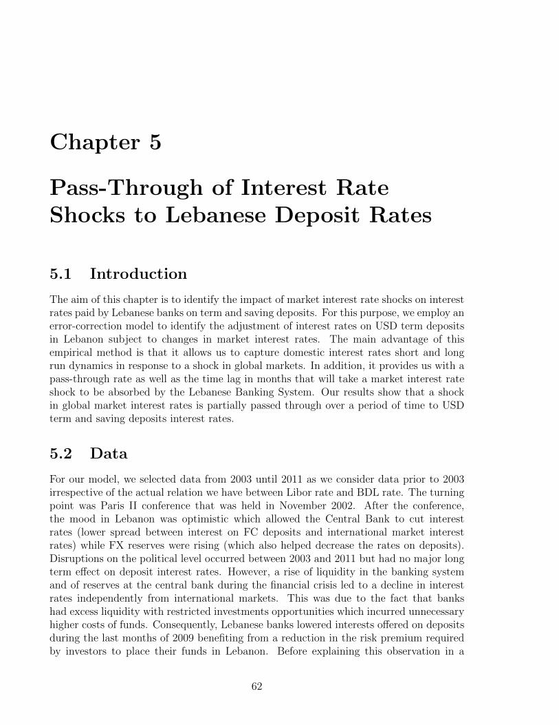
Chapter 5
Pass-Through of Interest RateShocks to Lebanese Deposit Rates
5.1 Introduction
The aim of this chapter is to identify the impact of market interest rate shocks on interestrates paid by Lebanese banks on term and saving deposits. For this purpose, we employ anerror-correction model to identify the adjustment of interest rates on USD term depositsin Lebanon subject to changes in market interest rates. The main advantage of thisempirical method is that it allows us to capture domestic interest rates short and longrun dynamics in response to a shock in global markets. In addition, it provides us with apass-through rate as well as the time lag in months that will take a market interest rateshock to be absorbed by the Lebanese Banking System. Our results show that a shockin global market interest rates is partially passed through over a period of time to USDterm and saving deposits interest rates.
5.2 Data
For our model, we selected data from 2003 until 2011 as we consider data prior to 2003irrespective of the actual relation we have between Libor rate and BDL rate. The turningpoint was Paris II conference that was held in November 2002. After the conference,the mood in Lebanon was optimistic which allowed the Central Bank to cut interestrates (lower spread between interest on FC deposits and international market interestrates) while FX reserves were rising (which also helped decrease the rates on deposits).Disruptions on the political level occurred between 2003 and 2011 but had no major longterm effect on deposit interest rates. However, a rise of liquidity in the banking systemand of reserves at the central bank during the financial crisis led to a decline in interestrates independently from international markets. This was due to the fact that bankshad excess liquidity with restricted investments opportunities which incurred unnecessaryhigher costs of funds. Consequently, Lebanese banks lowered interests offered on depositsduring the last months of 2009 benefiting from a reduction in the risk premium requiredby investors to place their funds in Lebanon. Before explaining this observation in a
62

Interest Rate Dynamics in the Lebanese Market Actuarial Thesis
quantitative way, we introduce the two variables used in the model.
5.2.1 Banking Sector Average Rate (BSAR)
The main variable of the model is the weighted average of term deposits interest rate inLebanon. The historical time series data is collected by the Lebanese Central Bank andis available on its official website 1. With respect to circular BDL18 issued by LebaneseCentral Bank in 1992, each Lebanese Bank should report monthly the below table.
Table 5.1: BSAR calculation
Monthly Average Weight
Interest Rate on Term DepositsInterest Rate on Current AccountsInterest Rate on Saving DepositsAccounts Maturity1 Month3 Months6 Months1 year and above
TOTAL 100%
Then, the central bank will calculate the weighted average using the following formula:
BSAR =
∑i(Customers’ Deposits)i × (Interest Rate)i∑
i(Customers’ Deposits)i
5.2.2 London InterBank Offered Rate (LIBOR)
LIBOR is a weighted average interest rate at which a selection of banks are preparedto lend one another unsecured funds on the London money market. The selection ofthe banks is made every year by the British Bankers’ Association with assistance fromthe Foreign Exchange and Money Markets Committee. The calculation of LIBOR is incharge of Thomson Reuters which collects the rates from all panel Banks then eliminatesthe highest and lowest 25% and calculates the weighted average of the mid values.We chose LIBOR as a proxy of market interest rates as it is known as the most importantbenchmark in the world for short-term interest rates. In addition to the fact that Banksuse LIBOR as the reference rate when pricing loans, savings and mortgages.
1Official website of the Lebanese Central Bank: www.bdl.gov.lb
63
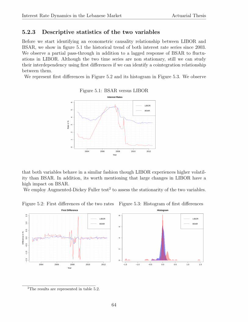
Interest Rate Dynamics in the Lebanese Market Actuarial Thesis
5.2.3 Descriptive statistics of the two variables
Before we start identifying an econometric causality relationship between LIBOR andBSAR, we show in figure 5.1 the historical trend of both interest rate series since 2003.We observe a partial pass-through in addition to a lagged response of BSAR to fluctu-ations in LIBOR. Although the two time series are non stationary, still we can studytheir interdependency using first differences if we can identify a cointegration relationshipbetween them.We represent first differences in Figure 5.2 and its histogram in Figure 5.3. We observe
Figure 5.1: BSAR versus LIBOR
2004 2006 2008 2010 2012
01
23
45
6
Interest Rates
Year
Rat
e in
%
LIBOR
BSAR
that both variables behave in a similar fashion though LIBOR experiences higher volatil-ity than BSAR. In addition, its worth mentioning that large changes in LIBOR have ahigh impact on BSAR.We employ Augmented-Dickey Fuller test2 to assess the stationarity of the two variables.
Figure 5.2: First differences of the two rates
2004 2006 2008 2010 2012
−1.
5−
1.0
−0.
50.
00.
51.
01.
5
First Difference
Year
Diff
eren
ce in
%
LIBOR
BSAR
Figure 5.3: Histogram of first differences
−1.5 −1.0 −0.5 0.0 0.5 1.0 1.5
02
46
8
Histogram
LIBOR
BSAR
2The results are represented in table 5.2.
64

Interest Rate Dynamics in the Lebanese Market Actuarial Thesis
Results show stationary in first differences. However, working with first differences wouldonly help determining short-run. Given that the aim of this paper is to model the long-runas well as the short-run relationships, we will need instead to employ an error correctionmodel to investigate interdependency between LIBOR and BSAR.
Table 5.2: Descriptive statistic of first differences
DBSAR Dlibor
Mean -0.01 -0.01STD 0.08 0.31VaR2.5% -0.22 -0.75Median -0.01 0.00VaR97.5% 0.10 0.30ADF(P-value) 0.01 <0.01
5.3 Error Correction model
5.3.1 Definition
The error-correction mechanism is a transformation of a general linear model3 incorpo-rating past values of both the explained variable (interest on term deposits in Lebanon)and the explanatory variables (LIBOR).An advantage of the error-correction model is that it provides explicitly the short termdeviations from long-run equilibrium in the estimated equation.This ECM will allow us to assess the following:
- Short term reaction of interest rates in response to a shock
- The long run equilibrium coefficients
- The speed of adjustment towards the long run equilibrium after a shock
This turns out to be very useful for the purpose of our study as we are modeling theelasticity and the time it takes for an interest rate shock in the market to be grasped andpriced by the Lebanese banking sector on customer deposits.This will allow us to assess the effective impact of an interest rate shock on the Bank’seconomic value of shareholders’ equity. Since customer deposits constitute the major partof our liabilities, a reduction and delay of an interest rate shock on these deposits inresponse to an shock in the market will reduce our interest rate risk (reduce Shareholders
3The details of the transformation is explained in Appendix F.1.
65
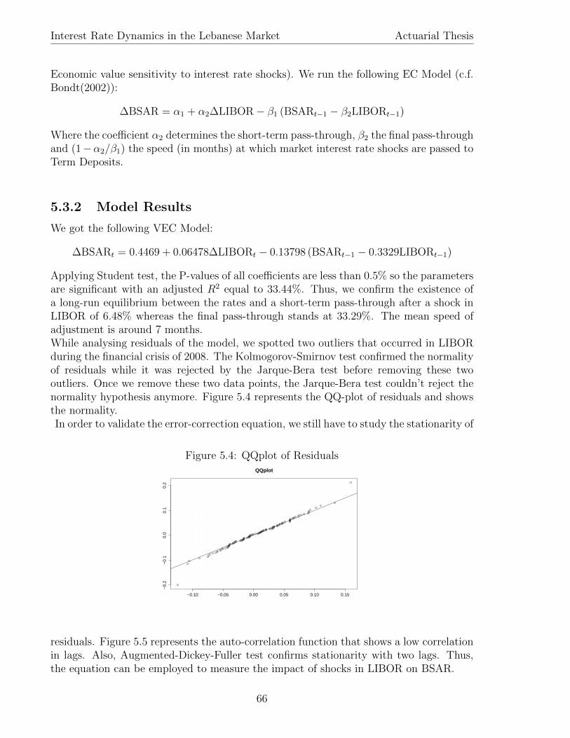
Interest Rate Dynamics in the Lebanese Market Actuarial Thesis
Economic value sensitivity to interest rate shocks). We run the following EC Model (c.f.Bondt(2002)):
∆BSAR = α1 + α2∆LIBOR− β1 (BSARt−1 − β2LIBORt−1)
Where the coefficient α2 determines the short-term pass-through, β2 the final pass-throughand (1−α2/β1) the speed (in months) at which market interest rate shocks are passed toTerm Deposits.
5.3.2 Model Results
We got the following VEC Model:
∆BSARt = 0.4469 + 0.06478∆LIBORt − 0.13798 (BSARt−1 − 0.3329LIBORt−1)
Applying Student test, the P-values of all coefficients are less than 0.5% so the parametersare significant with an adjusted R2 equal to 33.44%. Thus, we confirm the existence ofa long-run equilibrium between the rates and a short-term pass-through after a shock inLIBOR of 6.48% whereas the final pass-through stands at 33.29%. The mean speed ofadjustment is around 7 months.While analysing residuals of the model, we spotted two outliers that occurred in LIBORduring the financial crisis of 2008. The Kolmogorov-Smirnov test confirmed the normalityof residuals while it was rejected by the Jarque-Bera test before removing these twooutliers. Once we remove these two data points, the Jarque-Bera test couldn’t reject thenormality hypothesis anymore. Figure 5.4 represents the QQ-plot of residuals and showsthe normality.In order to validate the error-correction equation, we still have to study the stationarity of
Figure 5.4: QQplot of Residuals
−0.10 −0.05 0.00 0.05 0.10 0.15
−0.
2−
0.1
0.0
0.1
0.2
QQplot
residuals. Figure 5.5 represents the auto-correlation function that shows a low correlationin lags. Also, Augmented-Dickey-Fuller test confirms stationarity with two lags. Thus,the equation can be employed to measure the impact of shocks in LIBOR on BSAR.
66

Interest Rate Dynamics in the Lebanese Market Actuarial Thesis
Figure 5.5: Auto-Correlation Function of Residuals
0 5 10 15 20
−0.
20.
00.
20.
40.
60.
81.
0
Auto−Correlation Function
The most important step in the study is to draw the impulse response function. Weprovide a brief description of this function calculation in Appendix F.2. We represent theimpulse response function in Figure 5.6, that shows existence of a positive impact thatdecreases in value reaching 1 basis point after 12 months. On the other hand, Figure 5.7shows the convergence of BSAR to its long-run equilibrium.
Figure 5.6: Impulse Response Function
0 5 10 15 20
0.00
0.01
0.02
0.03
0.04
0.05
0.06
Impulse Response Function
Maturity in Months
Figure 5.7: Cumulative IRF
0 5 10 15 20
0.10
0.15
0.20
0.25
0.30
Cumulative Impulse Response Function
Maturity in Months
5.4 Shock Analysis
We represent in Table 5.3 the speed of adjustment. Results show that 86.44% of thelong-run effect will be grasped by the Lebanese Banking sector in the first year. We studythe impact of a 200 bps positive jump in LIBOR on BSAR and we obtain the following:
Short-Run: 0.0647× 200bps = 12.95bps
Impact after one year: 0.8644× 0.3329× 200bps = 57.56bps
67

Interest Rate Dynamics in the Lebanese Market Actuarial Thesis
Long-Run: 0.3329× 200bps = 66.58bps
Table 5.3: Distribution of the shock
Maturity % of the long-run Maturity % of the long-run
3 Months 48.41% 15 Months 91.31%6 Months 66.95% 18 Months 94.44%9 Months 78.83% 21 Months 96.44%
12 Months 86.44% 24 Months 97.72%
To be more conservative, we assume that the shock will be totally grasped in 12 monthsby the Lebanese Banking sector. Therefore, we shift the cumulative impulse responsefunction (divide all the number by 0.8644) to obtain the following curve which will beused to model the impact of a shock in LIBOR on the repricing of USD customers’deposits.
Figure 5.8: Behavior of BSAR in response of 200 bps changes in LIBOR
2 4 6 8 10 12
010
2030
4050
6070
Behavior of BSAR after 200 bps Shock in LIBOR
Maturity in Months
bps
estimated IRF
adjusted IRF
5.5 Application
As previously mentioned, we concentrate on Bank Audi’s customers deposits which con-stitute majority(80%-90%) of the bank’s liabilities. Main part of these deposits has acontractual maturity below or equal to 1 month. Though this is the simplest assump-tion for deposits’ repricing, it doesn’t however reflect their effective duration. In thissection, we formulate a methodology for rebucketing deposits according to their effectiverepricing that we got from our model. First of all, we consider the total shock is passedthrough within a 1 year horizon. As mentioned previously, our model estimates a totalpass-through of 33% from which 86% within a year time.To be more conservative, we will assume the following:
68

Interest Rate Dynamics in the Lebanese Market Actuarial Thesis
- The 33% will be totally passed through within the year horizon. We suppose that thelong-run is totally passed through within 1 year then we construct the cumulativeimpulse response function which converges to 100% instead of 86% (as detailedearlier).
- The remaining 67% will be passed through at the end of the year.
We will use the impulse response function; we developed earlier, to determine the per-centage of deposits that are repriced at each point in time. For example, if the impulseresponse function shows that 7% of the shock is passed through the first month, there-fore 7% of deposits will be repriced in 1 month. The remaining 93% are shifted to the2nd month where we redo this procedure until we reach the 1 year point where all theremaining deposits are assumed to reprice.This will yield us with the effective repricing of deposits which is higher than their con-tractual repricing. Therefore, the effective duration of our liabilities will be higher thanthe contractual duration which will lower the duration gap between assets and liabilitiesand as a result will lower the bank’s sensitivity to interest rate risk.We illustrate an application of the model in the below example summarized in table 5.5.
Table 5.4: Model Results
Maturity 1 Month 3 Months 6 Months 12 Months
1 7.69% - - -2 4.39% - - -3 3.78% 18.04% - -4 3.26% 3.71% - -5 2.81% 3.20% - -6 2.42% 2.76% 31.21% -7 2.09% 2.38% 2.68% -8 1.80% 2.05% 2.31% -9 1.55% 1.77% 1.99% -
10 1.34% 1.52% 1.71% -11 1.15% 1.31% 1.48% -12 67.70% 63.27% 58.63% 100.00%
We suppose a bank holds 2,500,000 USD as customers’ deposits distributed as representedin table 5.5. The present value of deposits without any adjustment is equal to USD2,487,491 whereas the adjusted present value declines to USD 2,429,173. The changein value of liabilities after a shock increased from -7,274 to -37,946. This shows thatliabilities sensitivity is higher and will compensate the decrease in value of assets after apositive shock in interest rates.4
4To understand the positive impact refer to the Appendix F.3
69
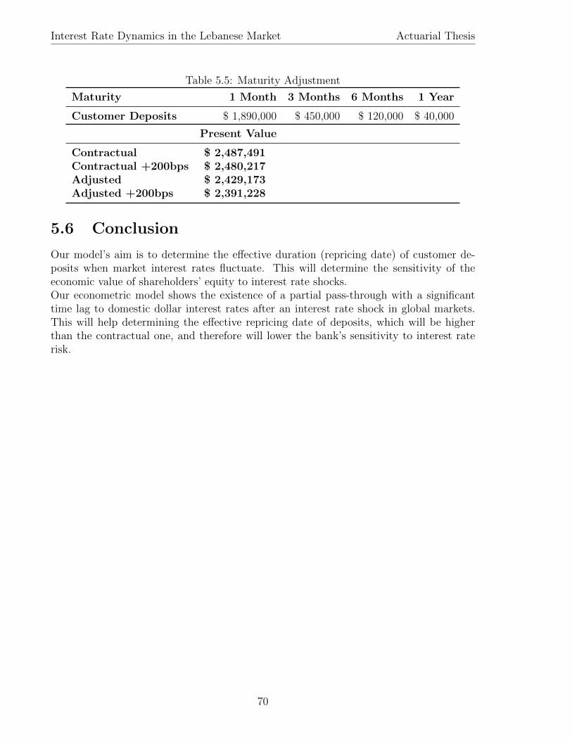
Interest Rate Dynamics in the Lebanese Market Actuarial Thesis
Table 5.5: Maturity Adjustment
Maturity 1 Month 3 Months 6 Months 1 Year
Customer Deposits $ 1,890,000 $ 450,000 $ 120,000 $ 40,000
Present Value
Contractual $ 2,487,491Contractual +200bps $ 2,480,217Adjusted $ 2,429,173Adjusted +200bps $ 2,391,228
5.6 Conclusion
Our model’s aim is to determine the effective duration (repricing date) of customer de-posits when market interest rates fluctuate. This will determine the sensitivity of theeconomic value of shareholders’ equity to interest rate shocks.Our econometric model shows the existence of a partial pass-through with a significanttime lag to domestic dollar interest rates after an interest rate shock in global markets.This will help determining the effective repricing date of deposits, which will be higherthan the contractual one, and therefore will lower the bank’s sensitivity to interest raterisk.
70

Interest Rate Dynamics in the Lebanese Market Actuarial Thesis
71

Chapter 6
Conclusion
Advanced Interest Rate models is here to stay as an important technique to understandinterest rate dynamics and manage its risk. In the first part, we showed the movement ofLBP yield curve in response to changing in political or economical situation whereas inthe second part, we modeled the response of US deposit offered rate to shock in LIBOR,also we showed how it can be used to adjust maturities for non-maturing liabilities inorder to determine the sensitivity of the economic value of shareholders’ equity to interestrate shocks.
The first model guided us to obtain more accurate value of the fixed income portfolioas well as to understand in-sample and out-of-sample LBP yield curve movements. Andthe second model helped us in determining the effective repricing date of deposits, whichwill be higher than the contractual one, and therefore will lower the bank’s sensitivity tointerest rate risk.
72

Interest Rate Dynamics in the Lebanese Market Actuarial Thesis
73

Bibliography
[1] Banerjee A., Dolado J., Galbraith J., Hendry D.(1993)Co-integration, er-ror Correction, and the econometric analysis of non-stationary data. Oxford Univer-sity Press.
[2] BIS Papers(2004) Principles for the management and supervision of interest raterisk. BIS Working Paper.
[3] BIS Papers(2005) Zero-coupon yield curves: technical documentation. BIS WorkingPaper.
[4] Bondt G.(2002) Retail bank interest rate pass-Through: new evidence at the euroarea level. European Central Bank Working Paper No 136.
[5] Brennan M., Schwartz E.(1979) A continuous time approach to the pricing ofbonds. Journal of Banking and Finance Volume 3 Issue 2, 133-155.
[6] Cox J., Ingersoll J., Ross S.(1985) A theory of the term structure of interestrates. Econometria, Volume 53, Issue 2, 285-408.
[7] Diebold F., Li C.(2006) Forecasting the term structure of government bond yields.Journal of Econometrics 130,337-364.
[8] Dothan L.(1978) On the term structure of interest rates. Journal of FinancialEconomics Volume 6 Issue 1, 58-69.
[9] Duffie D., Kan R.(1996) A yield-factor of interest rates. Mathematical FinanceVolume 6 No 4, 379-406.
[10] Feilitzen H.(2011) Modeling non-maturing liabilities. www.math.kth.se, thesis.
[11] Gilli M., Grobe S., Schumann E.(2010) Calibrating the Nelson-Siegel-Svenssonmodel. COMISEF Working Paper 031.
[12] Hamilton J.(1994) Time series analysis. Princeton University Press.
[13] Hana H.(2011) Nelson-Siegel model for the estimation of yield curve derived fromthe Czech coupon bond market. Journal of Applied Mathematics volume IV(2011),number III, 37-48.
[14] Hendry D.(1995)Dynamic econometrics. Oxford University Press.
74

Interest Rate Dynamics in the Lebanese Market Actuarial Thesis
[15] Hull J.(2012) Risk management and financial institutions. Wiley Finance.
[16] Letkepohl H.(2003) New introduction to multiple time series, Springer.
[17] Nelson C., Siegel A.(1987) Parsimonious modeling of yield curves. Journal ofBusiness, Volume 60, Issue 4, 473-489.
[18] Poddar T., Goswami M., Sole J., Echevarria-Icaza V.(2006) Interest ratedetermination in Lebanon. IMF working Paper, WP/06/94.
[19] Schmidt A.(2008) Paris trading: a cointegration approach. University of Sydney,Thesis.
[20] Sorensen C., Werner T.(2006) Bank interest rate pass-through in the euro area,a cross country comparison. European Central Bank Working Paper Series No 580.
[21] Svensson L.(1994) Estimating and interpreting forward interest rates: Sweden1992-1994. NBER Working Paper No 4871.
[22] Vasicek O.(1977) An equilibrium characterization of the term structure. Journal ofFinancial Economics 5, 177-188.
[23] Watson M.(1994) Vector autoregressions and cointegration. Handbook of Econo-metrics, Volume IV.
Other References
- Corm G., L’economie libanaise: risques et perspectives, www.georgescorm.com.
- Bloomberg: www.bloomberg.com.
- Lebanese Central Bank: www.bdl.gov.lb.
75

Appendix A
Fixed Income Portfolio Example
We consider a two-year 10% with a face value of $100. Suppose that the yield on the bondis 12% with continuous compounding and coupon payments of $2.5 are made every threemonths. The calculation of the duration and Convexity is represented in the table A.1.The table shows that the duration is equal to 1.833 whereas the convexity is equal to
Table A.1: Calculation of Duration and Convexity
Time Cash flow Present Value Weight Duration Convexity
0.25 $ 2.50 $ 2.4261 0.025 0.006 0.0000.50 $ 2.50 $ 2.3544 0.024 0.012 0.0030.75 $ 2.50 $ 2.2848 0.024 0.018 0.0101.00 $ 2.50 $ 2.2173 0.023 0.023 0.0231.25 $ 2.50 $ 2.1518 0.022 0.028 0.0441.50 $ 2.50 $ 2.0882 0.022 0.033 0.0731.75 $ 2.50 $ 2.0265 0.021 0.037 0.1132.00 $ 102.50 $ 80.6294 0.838 1.677 6.707
Total $ 120.00 $ 96.1784 1.000 1.833 6.973
6.973. So we have the following equation:
∆B = −96.1784× 1.833×∆y +1
2× 6.973× 96.1784× (∆y)2
We apply this formula to our example and we outlines results in the table A.2. The results
Table A.2: Impact of interest rate change on Bond Price
Real Change 1st order 2nd order
0.10% -0.176 -0.176 -0.1761.00% -1.746 -1.763 -1.729
show that it is more likely to introduce the convexity in case of high changes in interestrates.
76

Interest Rate Dynamics in the Lebanese Market Actuarial Thesis
77

Appendix B
Yield Curve Models in CentralBanks
Table B.1: Yield Curve Models in Central Banks
Centra Bank EstimationMethod
Minimised Er-ror
Availability(BIS)
Belgium Svensson orNelson-Siegel
Weighted Prices up to 16 years
Canada Merrill LynchExponentialSpline
Weighted Prices up to 30 years
Finland Nelson-Siegel Weighted Prices up to 12 yearsFrance Svensson or
Nelson-SiegelWeighted Prices up to 10 years
Germany Svensson Yields up to 10 yearsItaly Nelson-Siegel Weighted Prices up to 30 yearsJapan Smoothing
SplinesPrices up to 10 years
Norway Svensson Yields up to 10 yearsSpain Svensson Weighted Prices up to 10 yearsSweeden Smoothing
Splines andSvensson
Yields up to 10 years
Switzerland Svensson Yields up to 30 yearsUK VRP Yields up to 30 yearsUSA Smoothing
SplinesWeighted Pricesor Prices
up to 10 years
78

Interest Rate Dynamics in the Lebanese Market Actuarial Thesis
79

Appendix C
Principal Component AnalysisTables
Table C.1: Factor Loadings for USD Zero Yields
PC1 PC2 PC3 PC4 PC5 PC6 PC7 PC8 PC9 PC10
1M -0.52 -0.48 0.46 0.29 -0.32 -0.22 -0.15 -0.12 -0.08 -0.033M -0.33 -0.46 -0.04 -0.21 0.30 0.36 0.39 0.40 0.30 0.116M -0.10 -0.42 -0.43 -0.28 0.27 0.10 -0.21 -0.46 -0.43 -0.171Y 0.17 -0.35 -0.56 0.12 -0.21 -0.44 -0.25 0.21 0.37 0.182Y 0.32 -0.25 -0.17 0.50 -0.19 0.12 0.50 0.14 -0.35 -0.303Y 0.31 -0.19 0.14 0.39 0.16 0.35 -0.06 -0.41 0.16 0.494Y 0.27 -0.17 0.25 0.16 0.33 0.11 -0.37 0.06 0.28 -0.315Y 0.25 -0.16 0.25 -0.04 0.31 -0.19 -0.21 0.33 -0.16 -0.276Y 0.23 -0.15 0.22 -0.18 0.19 -0.33 0.10 0.16 -0.31 0.277Y 0.22 -0.15 0.18 -0.26 0.02 -0.30 0.29 -0.15 -0.05 0.328Y 0.22 -0.14 0.14 -0.29 -0.16 -0.12 0.27 -0.31 0.27 -0.149Y 0.21 -0.14 0.11 -0.30 -0.34 0.14 0.04 -0.16 0.27 -0.41
10Y 0.21 -0.14 0.09 -0.29 -0.49 0.45 -0.34 0.31 -0.27 0.26
% of Variance 0.576 0.371 0.036 0.013 0.003 0.001 0.000 0.000 0.000 0.000Cumulative % 0.576 0.948 0.984 0.997 0.999 1.000 1.000 1.000 1.000 1.000
80

Interest Rate Dynamics in the Lebanese Market Actuarial Thesis
Table C.2: Factor Loadings for LBP Zero Yields
PC1 PC2 PC3 PC4 PC5 PC6 PC7 PC8 PC9 PC10
1M 0.09 -0.04 -0.78 0.52 0.09 0.25 -0.12 0.13 -0.06 0.023M 0.07 0.25 -0.10 0.36 -0.49 -0.44 0.37 -0.41 0.21 -0.066M 0.08 0.29 0.13 0.06 -0.66 0.04 -0.31 0.51 -0.30 0.091Y 0.12 0.17 -0.21 -0.45 -0.34 0.62 -0.03 -0.34 0.29 -0.102Y 0.15 0.31 -0.41 -0.50 0.13 -0.25 0.42 0.13 -0.38 0.213Y 0.18 0.44 -0.11 -0.12 0.25 -0.32 -0.35 0.22 0.41 -0.454Y 0.24 0.40 0.13 0.12 0.23 0.00 -0.34 -0.29 0.06 0.485Y 0.29 0.27 0.22 0.20 0.18 0.20 0.03 -0.25 -0.36 0.056Y 0.33 0.11 0.20 0.17 0.11 0.23 0.28 0.06 -0.21 -0.417Y 0.37 -0.04 0.14 0.09 0.04 0.15 0.31 0.27 0.17 -0.168Y 0.40 -0.18 0.05 0.01 -0.02 0.02 0.17 0.25 0.34 0.309Y 0.42 -0.30 -0.03 -0.08 -0.08 -0.13 -0.07 0.03 0.17 0.34
10Y 0.44 -0.40 -0.11 -0.15 -0.13 -0.27 -0.35 -0.31 -0.34 -0.31
% of Variance 0.885 0.076 0.017 0.012 0.008 0.002 0.000 0.000 0.000 0.000Cumulative % 0.885 0.961 0.978 0.991 0.998 1.000 1.000 1.000 1.000 1.000
Table C.3: Factor Loadings for USD Zero Yields Basing on Observed Yields on LebaneseMarket
PC1 PC2 PC3 PC4 PC5 PC6 PC7 PC8 PC9 PC10
1M 0.78 -0.42 0.37 -0.25 -0.09 -0.02 0.04 -0.03 -0.02 -0.013M 0.54 0.20 -0.43 0.52 0.26 0.13 -0.25 0.20 0.13 0.066M 0.30 0.55 -0.27 -0.15 -0.22 -0.19 0.42 -0.40 -0.27 -0.141Y 0.09 0.56 0.16 -0.54 -0.03 0.04 -0.24 0.40 0.32 0.192Y 0.01 0.24 0.35 -0.07 0.57 0.28 -0.27 -0.24 -0.36 -0.363Y 0.01 0.12 0.32 0.17 0.43 -0.08 0.38 -0.23 0.19 0.554Y 0.01 0.11 0.27 0.23 0.14 -0.36 0.32 0.23 0.27 -0.235Y 0.01 0.12 0.24 0.23 -0.08 -0.42 -0.05 0.29 -0.12 -0.356Y 0.01 0.12 0.23 0.22 -0.22 -0.30 -0.31 0.03 -0.32 0.147Y 0.01 0.12 0.21 0.21 -0.29 -0.07 -0.33 -0.26 -0.09 0.348Y 0.01 0.11 0.21 0.20 -0.30 0.18 -0.15 -0.34 0.31 -0.019Y 0.01 0.11 0.20 0.20 -0.27 0.40 0.13 -0.10 0.38 -0.40
10Y 0.01 0.11 0.20 0.19 -0.21 0.51 0.36 0.45 -0.45 0.20
% of Variance 0.991 0.007 0.001 0.000 0.000 0.000 0.000 0.000 0.000 0.000Cumulative % 0.991 0.998 0.999 1.000 1.000 1.000 1.000 1.000 1.000 1.000
81

Appendix D
Stationarity Tools
D.1 A unit root process has a variance that depends
on time
We consider discrete time stochastic process xt and suppose that it can be written as anautoregressive process of order 1:
xt = a1xt−1 + εt
The process has a unit root when a1 = 1 since the characteristic equation is m− a1 = 0.Therefore, we have:
yt = yt−1 + εt
By repeated substitution, we can write yt = y0 +∑t
j=1 εj. Then the variance of yt is givenby:
VAR(yt) =t∑
j=1
σ2 = tσ2
The variance depends on t since VAR(y1) = σ2, while VAR(y2) = 2σ2.
D.2 If a process has a unit root then the process will
be non-stationary
We consider Xt as a process having a unit root and we assume that it can be written asan autoregressive process of order p.
Xt =
p∑i=1
aiXt−i + εt
where εt is a white noise. After rearranging the terms we obtain the following equation:
P∑i=0
aiXt−i = εt
82

Interest Rate Dynamics in the Lebanese Market Actuarial Thesis
We denote by B the backward operator, hence we have BXt = Xt−1 then:(p∑i=0
aiBi
)Xt = εt
As Xt is a unit process, the characteristic polynomial can be divided by (B − I) where Iis the identity matrix. Then we have the following equation:
(B − I)BXt = εt
If (B − I)B is invertible then Xt = [(B − I)B]−1εt is stationary. We proof that the lastproposition is incorrect by contradiction.We suppose that (B− I)−1 exist then BXt = (B− I)−1εt is stationary, on the other handwe have:
(B − I)BXt = εt
BBXt −BXt = εt
BXt = BXt−1 − εt
We calculate recursively and we obtain:
BXt = Bt−1ε1 −Bt−2ε2 − −Bεt−1 − εt
Then the variance of BXt depends on time t which means that BXt is non-stationary.
D.3 Student’s T-test
We consider the following regression equation:
Yt = α + βXt + εt
for t = 1, · · · , n. Once we have estimated the coefficients α and β, we aim to test ifthe slope β is equal to some specified value β0(often taken to be 0, in which case thehypothesis is that x and y are unrelated).Let:
• α and β be the least-squares estimators.
• SEhatα and SEβ be the standard errors of least-squares estimators.
We have:
SEβ =
√1
n−2∑n
i=1(Yi − yi)2√∑ni=1(xi − x)2
Then
t =β − β0SEβ
has a t-distribution with n-2 degrees of freedom if the null hypothesis is true.
83

Appendix E
Cointegration and ECM Tools
E.1 If the vector Xt has two components therefore
the number of linearly independent cointegrat-
ing vectors will be at most equal to one
We consider the simple vector auto-regression (VAR) model:yt = a11yt−1 + a12zt−1 + εytzt = a21yt−1 + a22zt−1 + εzt
Applying the lag operator on yt−1 and zt−1, and rearranging we get:yt = a11Lyt + a12Lzt + εytzt = a21Lyt + a22Lzt + εzt
(1− a11L)yt − a12Lzt = εyt−a21Lyt + (1− a12L)zt = εzt
Applying Cramer’s rule on the system and we obtain:yt = (1−a22L)εyt+a12Lεzt
(1−a11L)(1−a22L)−a12a21L2
zt = a21Lεyt+(1−a11L)εzt(1−a11L)(1−a22L)−a12a21L2
The equations have the same inverse characteristic equation:
(1− a11L)(1− a22L)− a12a21L2 = 0 and λ = 1/L
Then this implies that:
λ2 − (a11 + a22)λ+ (a11a22 − a12a21) = 0
Whereby the characteristic roots λ1 and λ2 determine the time paths of both variables.We will see in which case we have the two variables cointegrated of order (1,1).
84

Interest Rate Dynamics in the Lebanese Market Actuarial Thesis
• If (λ1, λ2) lie inside the unit circle then stable solutions for the series yt and ztexists and the variables are stationary. An important implication of this is thatthey cannot be cointegrated of order (1, 1).
• If either root lies outside the unit circle then we call that the solutions are explo-sive,we have
yt =(1− a22L)εyt + a12Lεzt
(1− a11L)(1− a22L)− a12a21L2=
(1− a22L)εyt + a12Lεzt(1− λ1L)(1− λ2L)
since λ1 and λ2 are the roots of the characteristic equation. If (1, 2) lie inside theunit circle then the solution is stable, however if either root lies outside the unitcircle then the system is explosive. Neither variable is difference stationary whichimplies that the variables cannot be cointegrated of order (1, 1).
• If a12 = a21 = 0, then yt = a11yt−1 + εytzt = a22zt−1 + εzt
And the solution is trivial.
• If a11 = a22 = 1, then the two variables have unit roots. Therefore 1 = 2 = 1 and
yt = yt−1 + a12zt−1 + εyt
This implies the two variables cannot be cointegrated of order (1, 1).
We have shown that the two variables cannot be cointegrated of order (1, 1) if the tworoots lies outside or inside the unit circle or if the two roots are equal to one. Thus for ytand zt to be cointegrated of order (1, 1), it is necessary for one characteristic root to beunity and the other less than unity in absolute value. For example, if |λ| = 1 then
yt =(1− a22L)εyt + a12Lεzt
(1− L)(1− λ2L)
Multiplying the right-hand side and the left-hand side by (1− L):
(1− L)yt =(1− a22L)εyt + a12Lεzt
1− λ2LOr
(1− L)yt = yt − Lyt= yt − yt−1= ∆yt
Then
∆yt =(1− a22L)εyt + a12Lεzt
1− λ2Lis stationary if |λ2| < 1. We apply these conditions on the coefficients:If |λ1| = 1 then:
1− (a11 + a22) + a11a22 − a12a21 = 0 (refer to the characteristic equation)
Hence, a11 = 1−a22−a12a211−a22 .
And if |λ2| < 1, then a11a22 − a12a21 < 1
85

Interest Rate Dynamics in the Lebanese Market Actuarial Thesis
E.2 Transformation of a simple VAR model to VECM
We consider a simple VAR model:yt = a11yt−1 + a12zt−1 + εytzt = a21yt−1 + a22zt−1 + εzt
By a simple calculation, we obtain:(∆yt∆zt
)=
(a11 − 1 a12a21 a22 − 1
)(yt−1zt−1
)+
(εytεzt
)We have
a11 − 1 =−a12a211− a22
Therefore ∆yt = −a12a21
1−a22 yt−1 + a12zt−1 + εyt∆zt = a21yt−1 + (1− a22)zt−1 + εzt
If a12a21 6= 0 then we can build the cointegrating vector with respect to either variable.In this case we build with respect to yt−1. And we obtain
∆yt = αy(yt−1 − βzt−1) + εyt∆zt = αz(yt−1 − βzt−1) + εzt
Where αy = −a12a21
1−a22αz = a21β = 1−a22
a21
We say that αy and αz determine the speed of adjustment to bring the system back toequilibrium and β show the long-run equilibrium between yt and zt.We introduce the lag of ∆yt and ∆zt, and we obtain the general form of the vector errorcorrection model:
∆yt = αy(yt−1 − βzt−1) + c11∆yt−1 + c12∆zt−1 + εyt∆zt = αz(yt−1 − βzt−1) + c21∆yt−1 + c22∆zt−1 + εzt
E.3 Johansen Procedure
We denote by yt a vector of k variables and we assume that yt can be written as a vectorautoregressive of order p.
yt = A1yt−1 + A2yt−2 + · · ·+ Apyt−p + εt
Where Ai is a k × k matrix (for every i = 1, · · · , p) and εt is a k × 1 white noise processcontaining the error terms. We reparametrize the VAR:
86

Interest Rate Dynamics in the Lebanese Market Actuarial Thesis
• Add and subtract Apyt−(p−1) from right-hand side
yt = A1yt−1 + A2yt−2 + · · ·+ Ap−1yt−(p−1) + (Ap − Ap)yt−(p−1) + Apyt−p + εt
yt = A1yt−1 + A2yt−2 + · · ·+ Ap−2yt−(p−2) + (Ap−1 + Ap)yt−(p−1) − Ap∆yt−(p−1) + εt
• Add and subtract (Ap−1 + Ap)yt−(p−1) from right-hand side
yt = A1yt−1+A2yt−2+· · ·+Ap−3yt−(p−3)+(Ap−2+Ap−1+Ap)yt−(p−2)−(Ap−1+Ap)∆yt−(p−2)
−Ap∆yt−(p−1) + εt
• By recurrence, we obtain:
yt = (A1+· · ·+Ap)yt−1−(A2+· · ·+Ap)∆yt−1−(A3+· · ·+Ap)∆yt−2−· · ·−Ap∆yt−p+εt
• We subtract yt−1 from left-hand side and right-hand side and we have
∆yt = −(I−A1−· · ·−Ap)yt−1−(A2+· · ·+Ap)∆yt−1−(A3+· · ·+Ap)∆yt−2−· · ·−Ap∆yt−p+εt
• Finally we conclude the generalized equation:
∆yt = −Πyt−1 +
p−1∑i=1
Φi∆yt−i + εt
Where Π = (I −∑n
i=1Ai) and Φi = −(∑n
j=i+1Aj).
E.4 If N variables can be written in N linearly inde-
pendent stationary equations, then the N vari-
ables are stationary.
Let yt = (y1t, · · · , yNt)′ be a vector of N variables. There exist N linearly independentcombinations of the components of yt such that the combinations are stationary. We canconclude that there exist a N ×N matrix A of rank equal to N and a stationary processεt = (ε1t, · · · , εNt)′ such that:
Ayt = εt
As the rank of A is equal to N then A−1 exists and we have:
yt = A−1εt
So all the components of yt can be written as a combination of stationary processes. Henceall the components of yt are integrated of order 0.
87

Appendix F
Error Correction ModelApplication’s Tools
F.1 Transformation of ADL(1,1) model to VEC model
We consider the autoregressive distributed lag model with a lag equal to 1:
BSARt = α0 + α1BSARt−1 + β0LIBORt + β1LIBORt−1 + εt
where ∀t ≥ 0, εt → N (0, σ2) and |α1| < 1. We suppose that we have a static equilibrium,noting that (BSARt,LIBORt) are jointly stationary, therefore we have the following long-run values: ∀t ≥ 0, E(BSARt) = BSAR∗ and E(LIBORt) = LIBOR∗. Since E(εt) = 0,we can write:
BSAR∗ =α0 + (β0 + β1)LIBOR∗
1− α1
= k0 + k1LIBOR∗
Hence, k1 = β0+β11−α1
is the long-run multiplier of term deposits interest rate with respectto libor. By a simple calculation, we obtain the equation of the vector error correctionmodel:
∆BSARt = α0 + (α1 − 1)(BSARt−1 − k1LIBORt−1) + β0∆LIBORt + εt
F.2 Impulse Response Function
In this part, we calculate the impulse response function of the following error correctionequation:
∆BSARt = α1 + α2∆LIBORt − β1(BSARt−1 − β2LIBORt−1)
⇐⇒ BSARt = α1 + (1− β1)BSARt−1 + α2LIBORt + (β1β2 − α2)LIBORt−1
In the following, we suppose that the shocked interest rate is indicated by the symbol ” ′
”. Therefore, if at time t LIBOR will increase ∆I in value, we have the following:
88

Interest Rate Dynamics in the Lebanese Market Actuarial Thesis
Time t: LIBOR′t − LIBORt = ∆IBSAR′t − BSARt = α2∆I
Time t+1:
BSAR′t+1 = α1 + (1− β1)BSAR′t + α2LIBORt+1 + (β1β2 − α2)LIBOR′t⇐⇒ BSAR′t+1 − BSARt+1 = (1− β1)α2∆I + (β1β2 − α2)∆I
Time t+2:
BSAR′t+2 = α1 + (1− β1)BSAR′t+1 + α2LIBORt+2 + (β1β2 − α2)LIBORt+1
⇐⇒ BSAR′t+2 − BSARt+2 = (1− β1)(BSAR′t+1 − BSARt+1)
We denote ut = BSAR′t − BSARt by the instantaneous impact of LIBOR on BSAR rateat time t and if LIBOR realizes a shock of ∆I at time 0 thus we have the following:
u0 = α2∆Iu1 = (1− β1)α2∆I + (β1β2 − α2)∆Iut+1 = (1− β1)ut
Therefore the cumulative impulse response function is calculated through the followingformula:
F (t) =t∑i=0
ui ∀i ∈ N
F.3 GAP Analysis
In banks, managers cope with interest rate risk arising from fluctuations in markets. Riskmanagers look at the income Gap Analysis as a measure of exposure to interest rate risk.Therefore, we measure the sensitivity of the bank’s interest income to changes in interestrates by using Gap Analysis:
GAP = RSA− RSL
Where RSA is rate sensitive short-term assets and RSL is rate sensitive short-term liabil-ities. The effect on bank income is given by:
∆I = GAP×∆i
Where ∆i denotes the change in interest rates. According to the circular number 250published by Banking Control Commission of Lebanon, we suppose that all interest rateswill increase by 200 bps.
89

List of Tables
1.1 Factor Loadings for EUR France Eurobond Yields . . . . . . . . . . . . . . 161.2 Standard Deviation of factor scores . . . . . . . . . . . . . . . . . . . . . . 171.3 Change of portfolio value for a 1 basis point rate move . . . . . . . . . . . 17
2.1 The term structure shapes resulting from all possible parameters constel-lations. . . . . . . . . . . . . . . . . . . . . . . . . . . . . . . . . . . . . . . 25
3.1 Distribution of the maturities . . . . . . . . . . . . . . . . . . . . . . . . . 333.2 Fitting Performance for different maturities . . . . . . . . . . . . . . . . . 41
5.1 BSAR calculation . . . . . . . . . . . . . . . . . . . . . . . . . . . . . . . . 635.2 Descriptive statistic of first differences . . . . . . . . . . . . . . . . . . . . 655.3 Distribution of the shock . . . . . . . . . . . . . . . . . . . . . . . . . . . . 685.4 Model Results . . . . . . . . . . . . . . . . . . . . . . . . . . . . . . . . . . 695.5 Maturity Adjustment . . . . . . . . . . . . . . . . . . . . . . . . . . . . . . 70
A.1 Calculation of Duration and Convexity . . . . . . . . . . . . . . . . . . . . 76A.2 Impact of interest rate change on Bond Price . . . . . . . . . . . . . . . . . 76
B.1 Yield Curve Models in Central Banks . . . . . . . . . . . . . . . . . . . . . 78
C.1 Factor Loadings for USD Zero Yields . . . . . . . . . . . . . . . . . . . . . 80C.2 Factor Loadings for LBP Zero Yields . . . . . . . . . . . . . . . . . . . . . 81C.3 Factor Loadings for USD Zero Yields Basing on Observed Yields on Lebanese
Market . . . . . . . . . . . . . . . . . . . . . . . . . . . . . . . . . . . . . . 81
90

Interest Rate Dynamics in the Lebanese Market Actuarial Thesis
91

List of Figures
2.1 β1 Loading Factor against First Component Factor (France Yield Curve) . 232.2 β2 Loading Factor against Second Component Factor(France Yield Curve) 232.3 β3 Loading Factor against third Component Factor(France Yield Curve) . . 24
3.1 Historical US Dollar Yield Curve (2009-2013). . . . . . . . . . . . . . . . . 293.2 Historical Lebanese Pound Yield Curve (2009-2013). . . . . . . . . . . . . . 293.3 Nelson-Sigel Loadings Correlation . . . . . . . . . . . . . . . . . . . . . . . 303.4 Svensson Loadings Correlation . . . . . . . . . . . . . . . . . . . . . . . . . 303.5 Histogram of Maturities for USD Bonds . . . . . . . . . . . . . . . . . . . 323.6 Histogram of Maturities for LBP Bonds . . . . . . . . . . . . . . . . . . . . 323.7 Nelson-Siegel Linear Parameters Behavior (β1,β2,β3) for US Dollar Yield
Curve . . . . . . . . . . . . . . . . . . . . . . . . . . . . . . . . . . . . . . 333.8 λ1, Adjusted R2, and Correlation between the two loadings factors for US
Dollar Yield Curve . . . . . . . . . . . . . . . . . . . . . . . . . . . . . . . 333.9 USD Nelson-Siegel Errors (R solution) . . . . . . . . . . . . . . . . . . . . 343.10 USD Nelson-Siegel Errors (Correlation Constraint Approach) . . . . . . . . 343.11 Time Series Errors of Nelson Siegel Model Applied on USD Curve . . . . . 353.12 QQplot Errors of Nelson Siegel Model Applied on USD Curve . . . . . . . 353.13 Auto Correlation Errors of Nelson Siegel Model Applied on USD Curve . . 353.14 Nelson-Siegel Linear Parameters Behaviour (β1,β2,β3) for US Dollar Yield
Curve . . . . . . . . . . . . . . . . . . . . . . . . . . . . . . . . . . . . . . 363.15 λ1, Adjusted R2, and Correlation between the two loadings factors for US
Dollar Yield Curve . . . . . . . . . . . . . . . . . . . . . . . . . . . . . . . 363.16 LBP Nelson-Siegel Errors (R solution) . . . . . . . . . . . . . . . . . . . . 373.17 LBP Nelson-Siegel Errors (Acceptable Correlation solution) . . . . . . . . . 373.18 Time Series Errors of Nelson Siegel Model Applied on LBP Curve . . . . . 373.19 QQplot Errors of Nelson Siegel Model Applied on LBP Curve . . . . . . . 373.20 Auto Correlation Errors of Nelson Siegel Model Applied on LBP Curve . . 373.21 Nelson-Siegel-Svensson Linear Parameters Behaviour (β1,β2,β3) for US Dol-
lar Yield Curve . . . . . . . . . . . . . . . . . . . . . . . . . . . . . . . . . 383.22 β4, λ1, Adjusted R2 for US yield curve . . . . . . . . . . . . . . . . . . . . 383.23 LBP Nelson-Siegel-Svensson Errors (R solution) . . . . . . . . . . . . . . . 393.24 LBP Nelson-Siegel-Svensson Errors (Acceptable Correlation solution) . . . 393.25 Time Series Errors of Nelson-Siegel-Svensson Model Applied on LBP Curve 393.26 QQplot Errors of Nelson-Siegel-Svensson Model Applied on LBP Curve . . 39
92
Interest Rate Dynamics in the Lebanese Market Actuarial Thesis
3.27 Auto Correlation Errors of Nelson-Siegel-Svensson Model Applied on LBPCurve . . . . . . . . . . . . . . . . . . . . . . . . . . . . . . . . . . . . . . 39
3.28 Nelson-Siegel-Svensson Linear Parameters Behaviour (β1,β2,β3) for LBPYield Curve . . . . . . . . . . . . . . . . . . . . . . . . . . . . . . . . . . . 40
3.29 β4, λ1, Adjusted R2 for LBP yield curve . . . . . . . . . . . . . . . . . . . 403.30 LBP Nelson-Siegel-Svensson Errors (R solution) . . . . . . . . . . . . . . . 403.31 LBP Nelson-Siegel-Svensson Errors (Acceptable Correlation solution) . . . 403.32 Time Series Errors of Nelson-Siegel-Svensson Model Applied on LBP Curve 403.33 QQplot Errors of Nelson-Siegel-Svensson Model Applied on LBP Curve . . 413.34 Auto Correlation Errors of Nelson-Siegel-Svensson Model Applied on LBP
Curve . . . . . . . . . . . . . . . . . . . . . . . . . . . . . . . . . . . . . . 413.35 Black: Adjusted R2 of the fitted LBP yield curve; Red: Adjusted R2 of the
fitted LBP yield curve using yields less than 7 years . . . . . . . . . . . . . 423.36 Adjusted R2 of the USD yield curve fitted only on observed Eurobonds
yields on the secondary Lebanese Market . . . . . . . . . . . . . . . . . . . 423.37 Component Factors (USD Yield Curve) compared to Nelson-Siegel-Svensson
loading factors . . . . . . . . . . . . . . . . . . . . . . . . . . . . . . . . . . 433.38 Component Factors (LBP Yield Curve) compared to Nelson-Siegel-Svensson
loading factors . . . . . . . . . . . . . . . . . . . . . . . . . . . . . . . . . . 443.39 Estimated Svensson Parameters using Constraint Correlation Approach
divided into 5 regimes. . . . . . . . . . . . . . . . . . . . . . . . . . . . . . 453.40 Lebanese Pound Fitted Yield Curve on 5 dates of different regimes. . . . . 45
5.1 BSAR versus LIBOR . . . . . . . . . . . . . . . . . . . . . . . . . . . . . . 645.2 First differences of the two rates . . . . . . . . . . . . . . . . . . . . . . . . 645.3 Histogram of first differences . . . . . . . . . . . . . . . . . . . . . . . . . . 645.4 QQplot of Residuals . . . . . . . . . . . . . . . . . . . . . . . . . . . . . . 665.5 Auto-Correlation Function of Residuals . . . . . . . . . . . . . . . . . . . . 675.6 Impulse Response Function . . . . . . . . . . . . . . . . . . . . . . . . . . 675.7 Cumulative IRF . . . . . . . . . . . . . . . . . . . . . . . . . . . . . . . . . 675.8 Behavior of BSAR in response of 200 bps changes in LIBOR . . . . . . . . 68
93