Determination of dynamic relative permeability in ultra

ORIGINAL PAPER - PRODUCTION ENGINEERING

Determination of dynamic relative permeability in ultra-lowpermeability sandstones via X-ray CT technique

Haiyong Zhang • Shunli He • Chunyan Jiao •

Guohua Luan • Shaoyuan Mo • Xuejing Guo

Received: 5 September 2013 / Accepted: 6 January 2014 / Published online: 20 January 2014

� The Author(s) 2014. This article is published with open access at Springerlink.com

Abstract Forced oil–water displacement is the crucial

mechanisms of secondary oil recovery. The knowledge of

relative permeability is required in the simulation of mul-

tiphase flow in porous media. Obvious dynamic effect of

capillary pressure occurs in that the formation of ultra-low

permeability reservoir (the permeability is \1 9

10-3 lm2) is tight and the pores and throats are very small.

In addition, the significant capillary end effect causes

serious errors when calculating relative permeabilities. For

these reasons, the JBN method (neglecting capillary pres-

sure) does not apply. Therefore, the dynamic capillary

pressure and capillary end effects should be taken into

account. This work focuses on calculating two-phase rel-

ative permeability of ultra-low permeability reservoir

through considering the dynamic capillary pressure and

eliminating the influence of capillary end effects. Firstly,

laboratory core scale measurements of in situ water phase

saturation history based on X-ray CT scanning technique

were used to estimate relative permeability. Secondly, a

mathematical model of two-phase relative permeability

considering the dynamic capillary pressure was estab-

lished. The basic problem formulations, as well as the more

specific equations, were given, and the results of

comparison using experimental data are presented and

discussed. Results indicate that the dynamic capillary

pressure measured at laboratory core scale in ultra-low

permeability rocks has a significant influence on the esti-

mation of unsteady-state relative permeability. The math-

ematical calculating method was compared with the history

matching method and the results were close, suggesting

reliability for ultra-low permeability reservoirs. Impor-

tantly, the proposed methods allow measurement of rela-

tive permeability from a single experiment. Potentially this

represents a great time savings.

Keywords Dynamic capillary effect � X-ray CT �Ultra-low permeability � Relative permeability

List of symbols

as Empirical constant, which is equal to 0.1

u Porosity (%)

uCT The CT-measured porosity (%)

lw Viscosity of the wetting phase (mPa s)

Pe& k Factors of capillary pressure–saturation

relationships in the Brook–Corey model

pcd The dynamic capillary pressure (MPa)

pce The steady-state capillary pressure (MPa)

po The capillary pressure of oil phase (MPa)

pw The capillary pressure of water phase (MPa)

ss or s The coefficient of dynamic capillary pressure

(kg m-1 s-1)

K Absolute permeability (10-3 lm2)

qw Density of the wetting phase (kg m-3)

g Gravity acceleration (m s-2)

L Characteristic length (cm)

D Diameter (cm)

Soi Initial oil saturation (%)

H. Zhang (&) � S. He � S. Mo � X. Guo

School of Petroleum Engineering, China University

of Petroleum, Beijing, China

e-mail: [email protected]

C. Jiao

Langfang Branch, CNPC Research Institute of Petroleum

Exploration and Development, Langfang, China

G. Luan

CNPC Petroleum Safety and Environmental Protection Institute

of Technology, Beijing, China

123

J Petrol Explor Prod Technol (2014) 4:443–455

DOI 10.1007/s13202-014-0101-6

Sor Residual oil saturation (%)

Swc Connate water saturation (%)

Krw (Sor) Relative permeability to water under residual

oil saturation, dimensionless

Kro (Swc) Relative permeability to oil under connate

water saturation, dimensionless

Kro Relative permeability to oil, dimensionless

Krw Relative permeability to water, dimensionless

uw Flow velocity of the wetting phase (cm s-1)

uz Injection velocity of the wetting phase at the

inlet end of core (cm s-1)

Kair Absolute permeability to air (10-3 lm2)

Kwat Absolute permeability to water (10-3 lm2)

EOR Oil recovery (%)

Swe Water saturation at the core outlet (%)

Swi Initial water saturation (%)

fo Oil ratio at the core outlet (%)

fw Water ratio at the core outlet (%)

I Injection ability at some time/the initial

injection ability

VoðtÞ Dimensionless cumulative oil production

volume

V tð Þ Dimensionless liquid production volume

CTDry The CT number for the dry core sample

CTAir The CT number for air

CTPhase1 The CT number for phase1

CTPhase2 The CT number for phase2

CTSaturated The CT number for the core saturated by one

single phase

CTTwo The CT number for two-phase liquids

CTGrain The CT number for the grain of core sample

CTow The CT number for the oil–water two phases

CTw The CT number for the water phase

CTo The CT number for the oil phase

CTor The CT number for the core sample saturated

by oil phase

Introduction

Simulation of multiphase flow in porous media requires

relative permeability functions to make estimates of pro-

ductivity, injectivity, and ultimate recovery from oil reser-

voirs for evaluation and planning of production operations

(Honarpour and Mahmood 1988). Hence, measurements of

relative permeability in the laboratory or theoretical models

remain an important subject in reservoir modeling.

The laboratory methods used to calculate relative per-

meability functions include centrifuge, steady- and

unsteady-state techniques. The centrifuge method has

limitations including loss of information on the low

saturation region that cannot be gained from the production

data at low mobility ratio (Hirasaki et al. 1995) and the

replacement of viscous forces with a range of centrifugal

forces for unsteady-state displacement processes that are

rate dependent was concerned (Ali 1997). Steady-state

methods have disadvantages, especially in the case of low

permeability rocks where it is laborious to reach multiple

steady states, and capillary pressures and capillary end

effects are significant (Firoozabadi and Aziz 1988; Kamath

et al. 1995; Huang and Honarpour 1998). Additionally, the

distribution of phases during the simultaneous injection of

fluids through the core may not represent the actual dis-

placement process in the reservoir.

The unsteady-state method is much less time consuming

than the steady-state method and is more representative of

the reservoir flow mechanisms, but the mathematical ana-

lysis of the unsteady-state procedure is more difficult and

the capillary pressure has a significant effect on saturation

distribution and recovery, capillary forces dominate mul-

tiphase flow in low-permeability rocks. Akin and Kovscek

(1999) indicated that the (unsteady) JBN technique

neglecting the capillary forces could lead to inaccurate

assessment of relative permeability in some cases. There-

fore, most conventional unsteady techniques do not apply.

There are also methods that infer relative permeability

by history matching observable parameters such as pres-

sure drop and saturation profile history. The relative per-

meability curves are adjusted until a good match is

obtained with the experimental data. The limitation is that

the description of the actual shape of the relative perme-

ability curves can cause errors (Hirasaki et al. 1995).

This work focuses on calculating two-phase dynamic

relative permeability of ultra-low permeability reservoir.

Firstly, the dynamic capillary pressure was investigated

through displacement tests and conventional mercury

injection tests. Secondly, the conventional JBN technique

was used to calculate two-phase relative permeability.

Results indicated that the JBN method did not apply.

Thirdly, laboratory core scale measurements of in situ

water phase saturation history via X-ray CT technique were

used to estimate relative permeability through history

matching method. Finally, a mathematical model of two-

phase relative permeability considering the dynamic cap-

illary pressure was established. The basic problem formu-

lations, as well as the more specific equations, were given

and the results of comparison with experiments are pre-

sented and discussed.

Dynamic capillary pressure

Dynamic capillary pressure refers to capillary pressure

relating to variation of wetting phase saturation as a

444 J Petrol Explor Prod Technol (2014) 4:443–455

123

function of time when the oil–water interface fails to reach

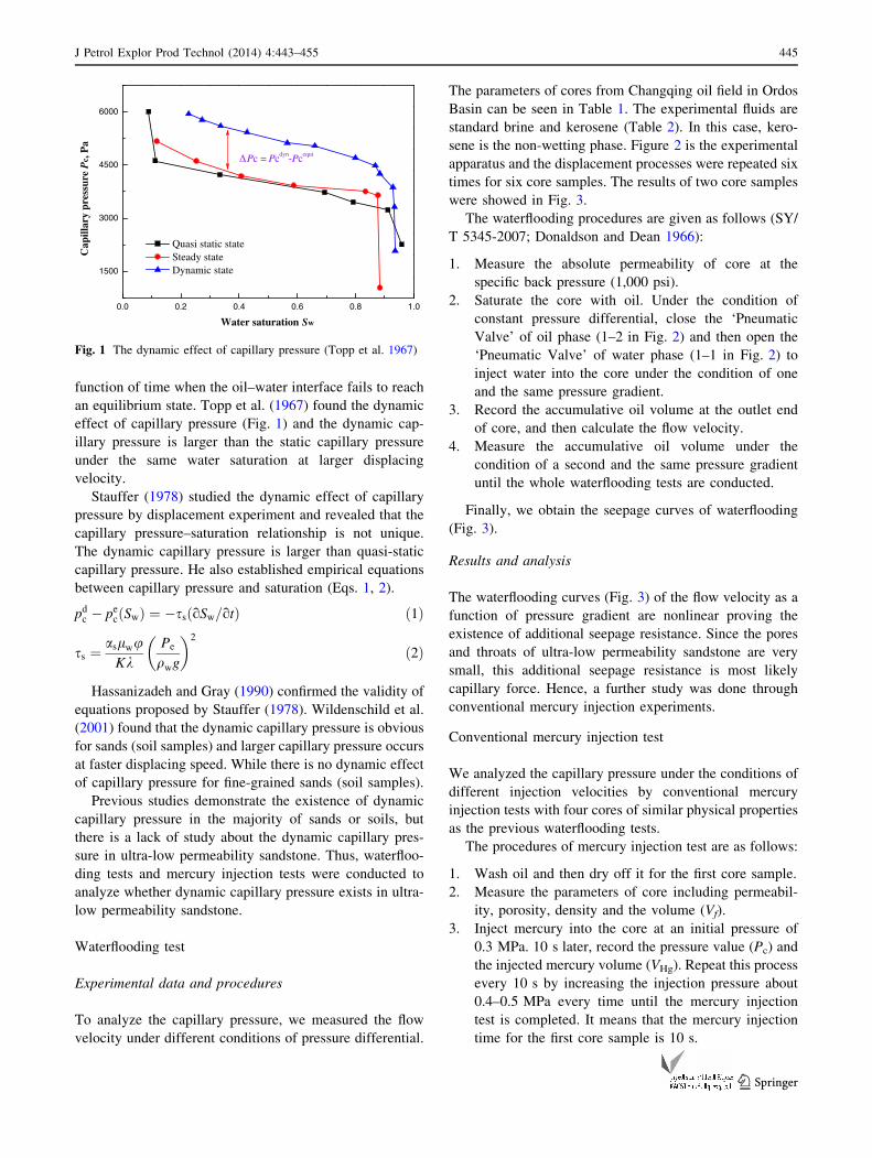
an equilibrium state. Topp et al. (1967) found the dynamic

effect of capillary pressure (Fig. 1) and the dynamic cap-

illary pressure is larger than the static capillary pressure

under the same water saturation at larger displacing

velocity.

Stauffer (1978) studied the dynamic effect of capillary

pressure by displacement experiment and revealed that the

capillary pressure–saturation relationship is not unique.

The dynamic capillary pressure is larger than quasi-static

capillary pressure. He also established empirical equations

between capillary pressure and saturation (Eqs. 1, 2).

pdc � pe

cðSwÞ ¼ �ssðoSw=otÞ ð1Þ

ss ¼aslwu

KkPe

qwg

� �2

ð2Þ

Hassanizadeh and Gray (1990) confirmed the validity of

equations proposed by Stauffer (1978). Wildenschild et al.

(2001) found that the dynamic capillary pressure is obvious

for sands (soil samples) and larger capillary pressure occurs

at faster displacing speed. While there is no dynamic effect

of capillary pressure for fine-grained sands (soil samples).

Previous studies demonstrate the existence of dynamic

capillary pressure in the majority of sands or soils, but

there is a lack of study about the dynamic capillary pres-

sure in ultra-low permeability sandstone. Thus, waterfloo-

ding tests and mercury injection tests were conducted to

analyze whether dynamic capillary pressure exists in ultra-

low permeability sandstone.

Waterflooding test

Experimental data and procedures

To analyze the capillary pressure, we measured the flow

velocity under different conditions of pressure differential.

The parameters of cores from Changqing oil field in Ordos

Basin can be seen in Table 1. The experimental fluids are

standard brine and kerosene (Table 2). In this case, kero-

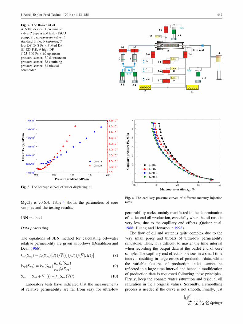
sene is the non-wetting phase. Figure 2 is the experimental

apparatus and the displacement processes were repeated six

times for six core samples. The results of two core samples

were showed in Fig. 3.

The waterflooding procedures are given as follows (SY/

T 5345-2007; Donaldson and Dean 1966):

1. Measure the absolute permeability of core at the

specific back pressure (1,000 psi).

2. Saturate the core with oil. Under the condition of

constant pressure differential, close the ‘Pneumatic

Valve’ of oil phase (1–2 in Fig. 2) and then open the

‘Pneumatic Valve’ of water phase (1–1 in Fig. 2) to

inject water into the core under the condition of one

and the same pressure gradient.

3. Record the accumulative oil volume at the outlet end

of core, and then calculate the flow velocity.

4. Measure the accumulative oil volume under the

condition of a second and the same pressure gradient

until the whole waterflooding tests are conducted.

Finally, we obtain the seepage curves of waterflooding

(Fig. 3).

Results and analysis

The waterflooding curves (Fig. 3) of the flow velocity as a

function of pressure gradient are nonlinear proving the

existence of additional seepage resistance. Since the pores

and throats of ultra-low permeability sandstone are very

small, this additional seepage resistance is most likely

capillary force. Hence, a further study was done through

conventional mercury injection experiments.

Conventional mercury injection test

We analyzed the capillary pressure under the conditions of

different injection velocities by conventional mercury

injection tests with four cores of similar physical properties

as the previous waterflooding tests.

The procedures of mercury injection test are as follows:

1. Wash oil and then dry off it for the first core sample.

2. Measure the parameters of core including permeabil-

ity, porosity, density and the volume (Vf).

3. Inject mercury into the core at an initial pressure of

0.3 MPa. 10 s later, record the pressure value (Pc) and

the injected mercury volume (VHg). Repeat this process

every 10 s by increasing the injection pressure about

0.4–0.5 MPa every time until the mercury injection

test is completed. It means that the mercury injection

time for the first core sample is 10 s.

0.0 0.2 0.4 0.6 0.8 1.0

1500

3000

4500

6000

Cap

illar

y pr

essu

re P

c , P

a

Water saturation Sw

Quasi static stateSteady stateDynamic state

Pc = Pcdyn-Pcequi

Fig. 1 The dynamic effect of capillary pressure (Topp et al. 1967)

J Petrol Explor Prod Technol (2014) 4:443–455 445

123

4. Calculate the mercury saturation (SHg) through the

following equation,

SHg ¼ VHg=ðuVf Þ ð3Þ

5. The mercury injection time for the other three core

samples is 60, 300 and 600 s, respectively. Repeat the

four procedures from step 1 to 4 and then, the capillary

pressure–mercury saturation relationships can be

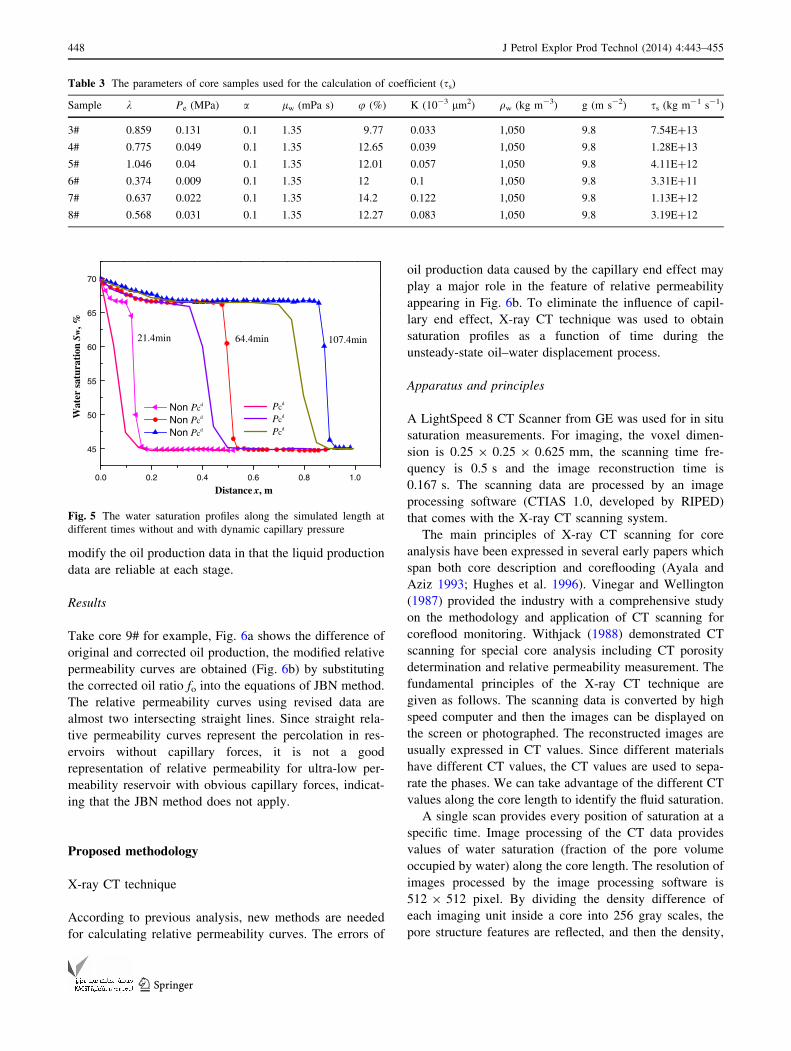
obtained in Fig. 4.

In Fig. 4, we see that the capillary pressure becomes

larger at a higher mercury injection velocity caused by

higher injection pressure. The capillary pressure differs

not quite when the mercury injection time is 300 and

600 s, indicating it can be approximately regarded as

static capillary pressure when the mercury injection time

reaches to 300 s (namely, the system reaches an equilib-

rium state).

We calculate the coefficient ss of ultra-low permeability

reservoir using Eq. 2, they can reach to 1011–

1013 kg m-1 s-1 (Table 3) while the coefficients ss cal-

culated by predecessors (Stauffer 1978; Wanna 1982;

Hassanizadeh and Gray 1990) are only 104–

107 kg m-1 s-1. Mirzaei and Das (2007) found that there

is a significant variation on the reported values of ss in the

literatures (0–109 kg m-1 s-1) depending on the size

(10-3–1 m) and geometry (2D or 3D) of domains. The

dynamic coefficient values up to 1011 kg m-1 s-1 were

found by Das et al. (2007) in their experiments on fine

sands with the permeability about 3 9 10-10 m2, which is

much larger than that of ultralow permeability core sample

(\1 9 10-3 lm2 or 1 9 10-15 m2). This indicates that the

coefficients ss are very big in ultra-low permeability res-

ervoir leading to obvious dynamic effect of capillary

pressure. The tighter the reservoir formation is, the larger

the coefficient ss will be. This result is in accordance with

the result of Das and Mirzaei (2012) where s is also found

to increase in the regions of less permeability.

Two-phase flow model

Then a two-phase flow model considering the dynamic

capillary pressure was established to analyze the influence

of dynamic capillary pressure on water saturation

distribution.

The dynamic capillary pressure is given by

po � pw ¼ pdc ¼ pe

c � sðoSw=otÞ ð4Þ

The basic differential equation of each phase is given as

follows. For the oil phase,

o

ox

KKro

lo

opo

ox

� �¼ u

oSo

otð5Þ

For the water phase,

o

ox

KKrw

lw

opw

ox

� �¼ u

oSw

otð6Þ

Thus substituting Eq. 5 into 6 and then combining with

4, the two-phase flow model is given by

o

ox

KKro

lo

o pw þ pec � sðoSw=otÞ

� �ox

� �þ o

ox

KKrw

lw

opw

ox

� �¼ 0

ð7Þ

The solution of the two-phase flow model was obtained

through the numerical method of implicit pressure–explicit

saturation (IMPES). The results can be seen in Fig. 5,

indicating that a reduction of forwarding velocity of water

saturation is induced considering the dynamic capillary

pressure and the existence of dynamic capillary pressure

has a significantly influence on the water saturation

distribution resulting in the smaller saturation gradient

and lower oil production.

Conventional methodology

Unsteady-state techniques

Laboratory equipment (Fig. 2) and procedures are avail-

able (see the previous section of waterflooding test) for

making the unsteady-state measurements under simulated

reservoir condition (SY/T 5345-2007; Donaldson and Dean

1966). Table 2 is the parameters of fluids. The salinity of

standard brine is 80 g/l, where the ratio of NaCl: CaCl2:

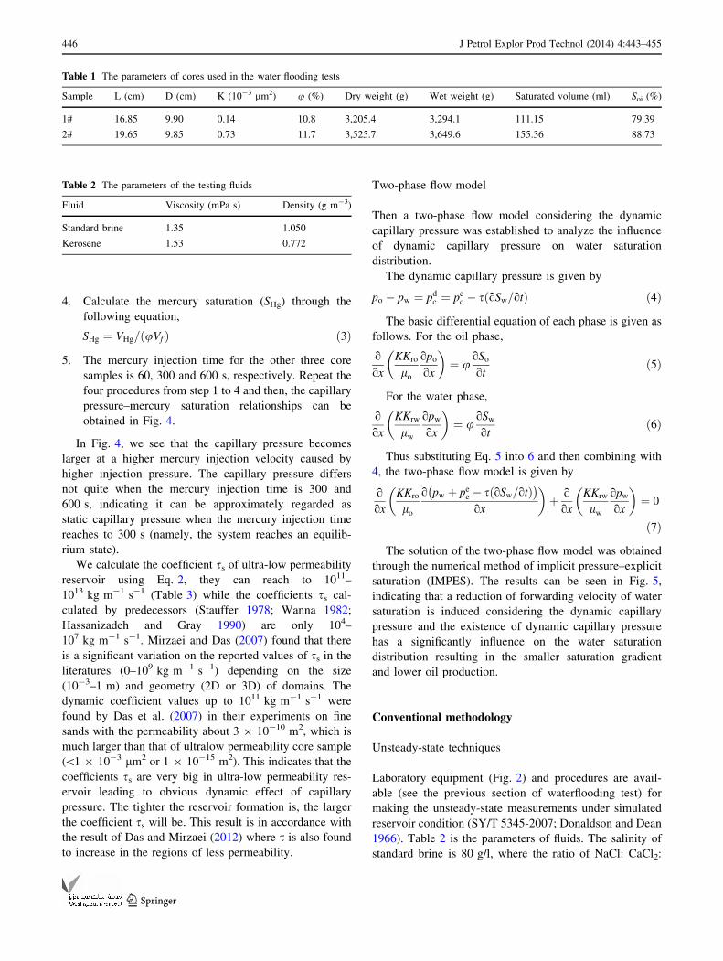
Table 1 The parameters of cores used in the water flooding tests

Sample L (cm) D (cm) K (10-3 lm2) u (%) Dry weight (g) Wet weight (g) Saturated volume (ml) Soi (%)

1# 16.85 9.90 0.14 10.8 3,205.4 3,294.1 111.15 79.39

2# 19.65 9.85 0.73 11.7 3,525.7 3,649.6 155.36 88.73

Table 2 The parameters of the testing fluids

Fluid Viscosity (mPa s) Density (g m-3)

Standard brine 1.35 1.050

Kerosene 1.53 0.772


123

MgCl2 is 70:6:4. Table 4 shows the parameters of core

samples and the testing results.

JBN method

Data processing

The equations of JBN method for calculating oil–water

relative permeability are given as follows (Donaldson and

Dean 1966):

kroðSweÞ ¼ foðSweÞ dð1=VðtÞÞ�

dð1=ðVðtÞIÞÞ� �

ð8Þ

krwðSweÞ ¼ kroðSweÞlw

lo

fwðSweÞfoðSweÞ

ð9Þ

Swe ¼ Swi þ VoðtÞ � foðSweÞVðtÞ ð10Þ

Laboratory tests have indicated that the measurements

of relative permeability are far from easy for ultra-low

permeability rocks, mainly manifested in the determination

of outlet end oil production, especially when the oil ratio is

very low, due to the capillary end effects (Qadeer et al.

1988; Huang and Honarpour 1998).

The flow of oil and water is quite complex due to the

very small pores and throats of ultra-low permeability

sandstone. Thus, it is difficult to master the time interval

when recording the output data at the outlet end of core

sample. The capillary end effect is obvious in a small time

interval resulting in large errors of production data, while

the variable features of production index cannot be

reflected in a large time interval and hence, a modification

of production data is requested following these principles.

Firstly, keep the connate water saturation and residual oil

saturation in their original values. Secondly, a smoothing

process is needed if the curve is not smooth. Finally, just

Fig. 2 The flowchart of

AFS300 device. 1 pneumatic

valve, 2 bypass and test, 3 ISCO

pump, 4 back-pressure valve, 5

standard brine, 6 kerosene, 7

low DP (0–8 Psi), 8 Med DP

(8–125 Psi), 9 high DP

(125–300 Psi), 10 upstream

pressure sensor, 11 downstream

pressure sensor, 12 confining

pressure sensor, 13 triaxial

coreholder

0.0 0.5 1.0 1.5 2.04.0x10-4

6.0x10-4

8.0x10-4

1.0x10-3

1.2x10-3

1.4x10-3

1.6x10-3

Core 1#Flo

w v

eloc

ity,

ml/m

in

Pressure gradient, MPa/m

Core 2#

0.0

2.0x10-3

4.0x10-3

6.0x10-3

8.0x10-3

1.0x10-2

1.2x10-2

1.4x10-2

1.6x10-2

1.8x10-2

Fig. 3 The seepage curves of water displacing oil90 80 70 60 50

0

1

2

3

4

5

6

7

t=10st=60st=300st=600s

Cap

illar

y pr

essu

re P

c , M

Pa

Mercury saturation SHg

, %

Fig. 4 The capillary pressure curves of different mercury injection

rates


123

modify the oil production data in that the liquid production

data are reliable at each stage.

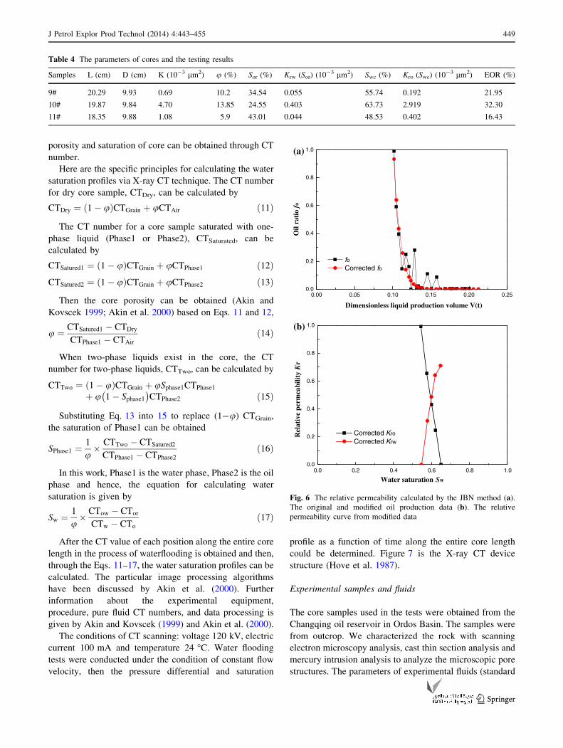
Results

Take core 9# for example, Fig. 6a shows the difference of

original and corrected oil production, the modified relative

permeability curves are obtained (Fig. 6b) by substituting

the corrected oil ratio fo into the equations of JBN method.

The relative permeability curves using revised data are

almost two intersecting straight lines. Since straight rela-

tive permeability curves represent the percolation in res-

ervoirs without capillary forces, it is not a good

representation of relative permeability for ultra-low per-

meability reservoir with obvious capillary forces, indicat-

ing that the JBN method does not apply.

Proposed methodology

X-ray CT technique

According to previous analysis, new methods are needed

for calculating relative permeability curves. The errors of

oil production data caused by the capillary end effect may

play a major role in the feature of relative permeability

appearing in Fig. 6b. To eliminate the influence of capil-

lary end effect, X-ray CT technique was used to obtain

saturation profiles as a function of time during the

unsteady-state oil–water displacement process.

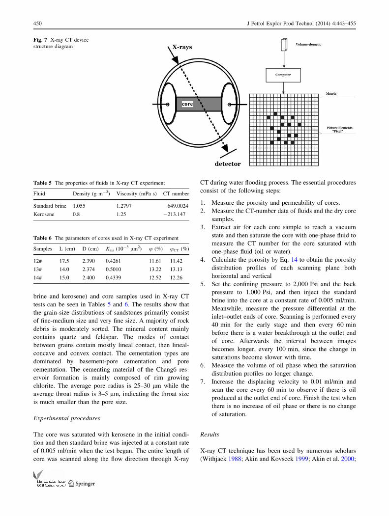
Apparatus and principles

A LightSpeed 8 CT Scanner from GE was used for in situ

saturation measurements. For imaging, the voxel dimen-

sion is 0.25 9 0.25 9 0.625 mm, the scanning time fre-

quency is 0.5 s and the image reconstruction time is

0.167 s. The scanning data are processed by an image

processing software (CTIAS 1.0, developed by RIPED)

that comes with the X-ray CT scanning system.

The main principles of X-ray CT scanning for core

analysis have been expressed in several early papers which

span both core description and coreflooding (Ayala and

Aziz 1993; Hughes et al. 1996). Vinegar and Wellington

(1987) provided the industry with a comprehensive study

on the methodology and application of CT scanning for

coreflood monitoring. Withjack (1988) demonstrated CT

scanning for special core analysis including CT porosity

determination and relative permeability measurement. The

fundamental principles of the X-ray CT technique are

given as follows. The scanning data is converted by high

speed computer and then the images can be displayed on

the screen or photographed. The reconstructed images are

usually expressed in CT values. Since different materials

have different CT values, the CT values are used to sepa-

rate the phases. We can take advantage of the different CT

values along the core length to identify the fluid saturation.

A single scan provides every position of saturation at a

specific time. Image processing of the CT data provides

values of water saturation (fraction of the pore volume

occupied by water) along the core length. The resolution of

images processed by the image processing software is

512 9 512 pixel. By dividing the density difference of

each imaging unit inside a core into 256 gray scales, the

pore structure features are reflected, and then the density,

Table 3 The parameters of core samples used for the calculation of coefficient (ss)

Sample k Pe (MPa) a lw (mPa s) u (%) K (10-3 lm2) qw (kg m-3) g (m s-2) ss (kg m-1 s-1)

3# 0.859 0.131 0.1 1.35 9.77 0.033 1,050 9.8 7.54E?13

4# 0.775 0.049 0.1 1.35 12.65 0.039 1,050 9.8 1.28E?13

5# 1.046 0.04 0.1 1.35 12.01 0.057 1,050 9.8 4.11E?12

6# 0.374 0.009 0.1 1.35 12 0.1 1,050 9.8 3.31E?11

7# 0.637 0.022 0.1 1.35 14.2 0.122 1,050 9.8 1.13E?12

8# 0.568 0.031 0.1 1.35 12.27 0.083 1,050 9.8 3.19E?12

0.0 0.2 0.4 0.6 0.8 1.0

45

50

55

60

65

70

107.4min64.4min21.4min

Wat

er s

atur

atio

n S w

, %

Distance x, m

Non Pcd

Non Pcd

Non Pcd

Pcd

Pcd

Pcd

Fig. 5 The water saturation profiles along the simulated length at

different times without and with dynamic capillary pressure


123

porosity and saturation of core can be obtained through CT

number.

Here are the specific principles for calculating the water

saturation profiles via X-ray CT technique. The CT number

for dry core sample, CTDry, can be calculated by

CTDry ¼ ð1 � uÞCTGrain þ uCTAir ð11Þ

The CT number for a core sample saturated with one-

phase liquid (Phase1 or Phase2), CTSaturated, can be

calculated by

CTSatured1 ¼ 1 � uð ÞCTGrain þ uCTPhase1 ð12ÞCTSatured2 ¼ 1 � uð ÞCTGrain þ uCTPhase2 ð13Þ

Then the core porosity can be obtained (Akin and

Kovscek 1999; Akin et al. 2000) based on Eqs. 11 and 12,

u ¼ CTSatured1 � CTDry

CTPhase1 � CTAir

ð14Þ

When two-phase liquids exist in the core, the CT

number for two-phase liquids, CTTwo, can be calculated by

CTTwo ¼ 1 � uð ÞCTGrain þ uSphase1CTPhase1

þ u 1 � Sphase1

� �CTPhase2 ð15Þ

Substituting Eq. 13 into 15 to replace (1-u) CTGrain,

the saturation of Phase1 can be obtained

SPhase1 ¼ 1

u� CTTwo � CTSatured2

CTPhase1 � CTPhase2

ð16Þ

In this work, Phase1 is the water phase, Phase2 is the oil

phase and hence, the equation for calculating water

saturation is given by

Sw ¼ 1

u� CTow � CTor

CTw � CTo

ð17Þ

After the CT value of each position along the entire core

length in the process of waterflooding is obtained and then,

through the Eqs. 11–17, the water saturation profiles can be

calculated. The particular image processing algorithms

have been discussed by Akin et al. (2000). Further

information about the experimental equipment,

procedure, pure fluid CT numbers, and data processing is

given by Akin and Kovscek (1999) and Akin et al. (2000).

The conditions of CT scanning: voltage 120 kV, electric

current 100 mA and temperature 24 �C. Water flooding

tests were conducted under the condition of constant flow

velocity, then the pressure differential and saturation

profile as a function of time along the entire core length

could be determined. Figure 7 is the X-ray CT device

structure (Hove et al. 1987).

Experimental samples and fluids

The core samples used in the tests were obtained from the

Changqing oil reservoir in Ordos Basin. The samples were

from outcrop. We characterized the rock with scanning

electron microscopy analysis, cast thin section analysis and

mercury intrusion analysis to analyze the microscopic pore

structures. The parameters of experimental fluids (standard

Table 4 The parameters of cores and the testing results

Samples L (cm) D (cm) K (10-3 lm2) u (%) Sor (%) Krw (Sor) (10-3 lm2) Swc (%) Kro (Swc) (10-3 lm2) EOR (%)

9# 20.29 9.93 0.69 10.2 34.54 0.055 55.74 0.192 21.95

10# 19.87 9.84 4.70 13.85 24.55 0.403 63.73 2.919 32.30

11# 18.35 9.88 1.08 5.9 43.01 0.044 48.53 0.402 16.43

0.00 0.05 0.10 0.15 0.20 0.250.0

0.2

0.4

0.6

0.8

1.0

Oil

rati

o f o

Dimensionless liquid production volume V(t)

fo Corrected fo

(a)

0.0 0.2 0.4 0.6 0.8 1.00.0

0.2

0.4

0.6

0.8

1.0

Rel

ativ

e pe

rmea

bilit

y K

r

Water saturation Sw

Corrected Kro

Corrected Krw

(b)

Fig. 6 The relative permeability calculated by the JBN method (a).

The original and modified oil production data (b). The relative

permeability curve from modified data


123

brine and kerosene) and core samples used in X-ray CT

tests can be seen in Tables 5 and 6. The results show that

the grain-size distributions of sandstones primarily consist

of fine-medium size and very fine size. A majority of rock

debris is moderately sorted. The mineral content mainly

contains quartz and feldspar. The modes of contact

between grains contain mostly lineal contact, then lineal-

concave and convex contact. The cementation types are

dominated by basement-pore cementation and pore

cementation. The cementing material of the Chang6 res-

ervoir formation is mainly composed of rim growing

chlorite. The average pore radius is 25–30 lm while the

average throat radius is 3–5 lm, indicating the throat size

is much smaller than the pore size.

Experimental procedures

The core was saturated with kerosene in the initial condi-

tion and then standard brine was injected at a constant rate

of 0.005 ml/min when the test began. The entire length of

core was scanned along the flow direction through X-ray

CT during water flooding process. The essential procedures

consist of the following steps:

1. Measure the porosity and permeability of cores.

2. Measure the CT-number data of fluids and the dry core

samples.

3. Extract air for each core sample to reach a vacuum

state and then saturate the core with one-phase fluid to

measure the CT number for the core saturated with

one-phase fluid (oil or water).

4. Calculate the porosity by Eq. 14 to obtain the porosity

distribution profiles of each scanning plane both

horizontal and vertical

5. Set the confining pressure to 2,000 Psi and the back

pressure to 1,000 Psi, and then inject the standard

brine into the core at a constant rate of 0.005 ml/min.

Meanwhile, measure the pressure differential at the

inlet–outlet ends of core. Scanning is performed every

40 min for the early stage and then every 60 min

before there is a water breakthrough at the outlet end

of core. Afterwards the interval between images

becomes longer, every 100 min, since the change in

saturations become slower with time.

6. Measure the volume of oil phase when the saturation

distribution profiles no longer change.

7. Increase the displacing velocity to 0.01 ml/min and

scan the core every 60 min to observe if there is oil

produced at the outlet end of core. Finish the test when

there is no increase of oil phase or there is no change

of saturation.

Results

X-ray CT technique has been used by numerous scholars

(Withjack 1988; Akin and Kovscek 1999; Akin et al. 2000;

Fig. 7 X-ray CT device

structure diagram

Table 5 The properties of fluids in X-ray CT experiment

Fluid Density (g m-3) Viscosity (mPa s) CT number

Standard brine 1.055 1.2797 649.0024

Kerosene 0.8 1.25 -213.147

Table 6 The parameters of cores used in X-ray CT experiment

Samples L (cm) D (cm) Kair (10-3 lm2) u (%) uCT (%)

12# 17.5 2.390 0.4261 11.61 11.42

13# 14.0 2.374 0.5010 13.22 13.13

14# 15.0 2.400 0.4339 12.52 12.26


123

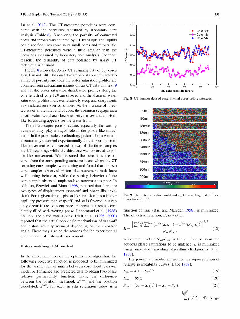
Lu et al. 2012). The CT-measured porosities were com-

pared with the porosities measured by laboratory core

analysis (Table 6). Since only the porosity of connected

pores and throats was counted by CT technique and liquids

could not flow into some very small pores and throats, the

CT-measured porosities were a little smaller than the

porosities measured by laboratory core analysis. For these

reasons, the reliability of data obtained by X-ray CT

technique is ensured.

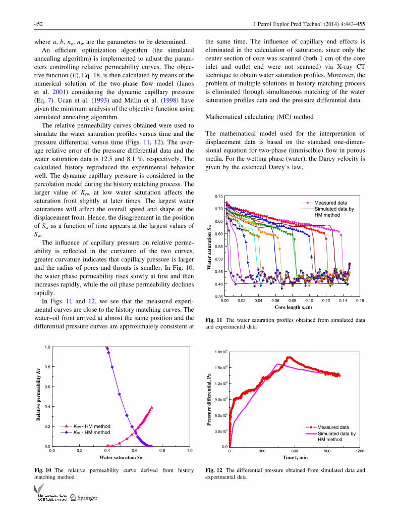
Figure 8 shows the X-ray CT scanning data of dry cores

12#, 13# and 14#. The raw CT-number data are converted to

a map of porosity and then the water saturation profiles are

obtained from subtracting images of raw CT data. In Figs. 9

and 11, the water saturation distribution profiles along the

core length of core 12# are showed and the shape of water

saturation profiles indicates relatively steep and sharp fronts

in simulated reservoir conditions. As the increase of injec-

ted water at the inlet end of core, the common seepage area

of oil–water two phases becomes very narrow and a piston-

like forwarding appears for the water front.

The microscopic pore structure, especially the sorting

behavior, may play a major role in the piston-like move-

ment. In the pore-scale coreflooding, piston-like movement

is commonly observed experimentally. In this work, piston-

like movement was observed in two of the three samples

via CT scanning, while the third one was observed unpis-

ton-like movement. We measured the pore structures of

cores from the corresponding same positions where the CT

scanning core samples were coring and found that the two

core samples observed piston-like movement both have

well-sorting behavior, while the sorting behavior of the

core sample observed unpiston-like movement is poor. In

addition, Fenwick and Blunt (1998) reported that there are

two types of displacement (snap-off and piston-like inva-

sion). For a given throat, piston-like invasion has a higher

capillary pressure than snap-off, and so is favored, but can

only occur if the adjacent pore or throat is already com-

pletely filled with wetting phase. Lenormand et al. (1988)

obtained the same conclusions. Dixit et al. (1998, 2000)

reported that the actual pore-scale mechanisms of snap-off

and piston-like displacement depending on their contact

angle. These may also be the reasons for the experimental

phenomenon of piston-like movement.

History matching (HM) method

In the implementation of the optimization algorithm, the

following objective function is proposed to be minimized

for the verification of match between core flood reservoir

model performance and predicted data to obtain two-phase

relative permeability function. Thus, the difference

between the position measured, xmeas, and the position

calculated, xcalc, for each in situ saturation value as a

function of time (Bail and Marsden 1956), is minimized.

The objective function, E, is written

E ¼PNprof

i¼0

PNsat

j¼1 ðxcalcðSwj; tiÞ � xmeasðSwj; tiÞÞ2

h i1=2

NsatNprof

ð18Þ

where the product NsatNprof is the number of measured

aqueous phase saturations to be matched. E is minimized

using simulated annealing algorithm (Kirkpatrick et al.

1983).

The power law model is used for the representation of

relative permeability curves (Lake 1989),

Kro ¼ að1 � SweÞno ð19ÞKrw ¼ bSnw

we ð20Þ

Swe ¼ ðSw � SwiÞ=ð1 � Sor � SwiÞ ð21Þ

0 20 40 60 80 1001700

1800

1900

2000

2100

2200

2300

CT

-num

ber

The axial scanning layers

Core 12# Core 13# Core 14#

Fig. 8 CT-number data of experimental cores before saturated

120min

180min

300min

540min

660min

780min

900min

80min

40min

1000min

Fig. 9 The water saturation profiles along the core length at different

times for core 12#


123

where a, b, no, nw are the parameters to be determined.

An efficient optimization algorithm (the simulated

annealing algorithm) is implemented to adjust the param-

eters controlling relative permeability curves. The objec-

tive function (E), Eq. 18, is then calculated by means of the

numerical solution of the two-phase flow model (Janos

et al. 2001) considering the dynamic capillary pressure

(Eq. 7). Ucan et al. (1993) and Mitlin et al. (1998) have

given the minimum analysis of the objective function using

simulated annealing algorithm.

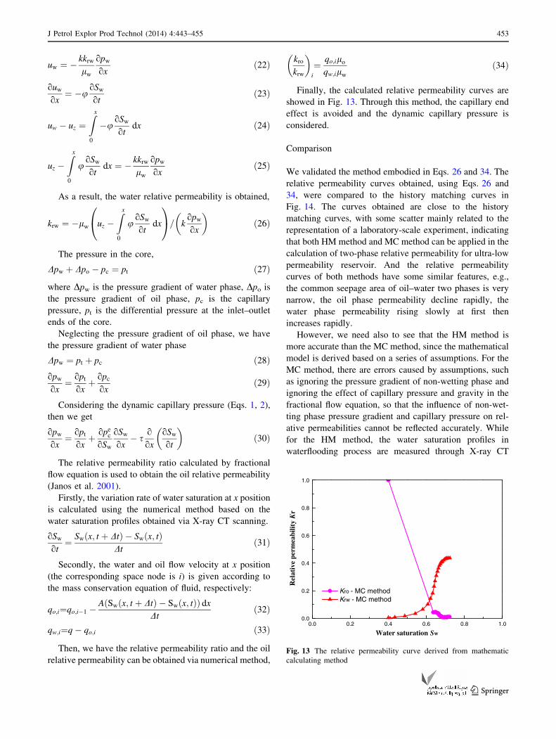
The relative permeability curves obtained were used to

simulate the water saturation profiles versus time and the

pressure differential versus time (Figs. 11, 12). The aver-

age relative error of the pressure differential data and the

water saturation data is 12.5 and 8.1 %, respectively. The

calculated history reproduced the experimental behavior

well. The dynamic capillary pressure is considered in the

percolation model during the history matching process. The

larger value of Krw at low water saturation affects the

saturation front slightly at later times. The largest water

saturations will affect the overall speed and shape of the

displacement front. Hence, the disagreement in the position

of Sw as a function of time appears at the largest values of

Sw.

The influence of capillary pressure on relative perme-

ability is reflected in the curvature of the two curves,

greater curvature indicates that capillary pressure is larger

and the radius of pores and throats is smaller. In Fig. 10,

the water phase permeability rises slowly at first and then

increases rapidly, while the oil phase permeability declines

rapidly.

In Figs. 11 and 12, we see that the measured experi-

mental curves are close to the history matching curves. The

water–oil front arrived at almost the same position and the

differential pressure curves are approximately consistent at

the same time. The influence of capillary end effects is

eliminated in the calculation of saturation, since only the

center section of core was scanned (both 1 cm of the core

inlet and outlet end were not scanned) via X-ray CT

technique to obtain water saturation profiles. Moreover, the

problem of multiple solutions in history matching process

is eliminated through simultaneous matching of the water

saturation profiles data and the pressure differential data.

Mathematical calculating (MC) method

The mathematical model used for the interpretation of

displacement data is based on the standard one-dimen-

sional equation for two-phase (immiscible) flow in porous

media. For the wetting phase (water), the Darcy velocity is

given by the extended Darcy’s law,

0.0 0.2 0.4 0.6 0.8 1.00.0

0.2

0.4

0.6

0.8

1.0

Rel

ativ

e pe

rmea

bilit

y K

r

Water saturation Sw

Krw - HM methodKro - HM method

Fig. 10 The relative permeability curve derived from history

matching method

0.00 0.02 0.04 0.06 0.08 0.10 0.12 0.14 0.160.35

0.40

0.45

0.50

0.55

0.60

0.65

0.70

0.75

Simulated data by HM method

Wat

er s

atur

atio

n Sw

Core length x,cm

Measured data

Fig. 11 The water saturation profiles obtained from simulated data

and experimental data

0 300 600 900 12000.0

3.0x105

6.0x105

9.0x105

1.2x106

1.5x106

1.8x106

Pre

ssur

e di

ffer

enti

al, P

a

Time t, min

Simulated data by HM method

Measured data

Fig. 12 The differential pressure obtained from simulated data and

experimental data


123

uw ¼ � kkrw

lw

opw

oxð22Þ

ouw

ox¼ �u

oSw

otð23Þ

uw � uz ¼Zx

0

�uoSw

otdx ð24Þ

uz �Zx

0

uoSw

otdx ¼ � kkrw

lw

opw

oxð25Þ

As a result, the water relative permeability is obtained,

krw ¼ �lw uz �Zx

0

uoSw

otdx

0@

1A= k

opw

ox

� �ð26Þ

The pressure in the core,

Dpw þ Dpo � pc ¼ pt ð27Þ

where Dpw is the pressure gradient of water phase, Dpo is

the pressure gradient of oil phase, pc is the capillary

pressure, pt is the differential pressure at the inlet–outlet

ends of the core.

Neglecting the pressure gradient of oil phase, we have

the pressure gradient of water phase

Dpw ¼ pt þ pc ð28Þopw

ox¼ opt

oxþ opc

oxð29Þ

Considering the dynamic capillary pressure (Eqs. 1, 2),

then we get

opw

ox¼ opt

oxþ ope

c

oSw

oSw

ox� s

o

ox

oSw

ot

� �ð30Þ

The relative permeability ratio calculated by fractional

flow equation is used to obtain the oil relative permeability

(Janos et al. 2001).

Firstly, the variation rate of water saturation at x position

is calculated using the numerical method based on the

water saturation profiles obtained via X-ray CT scanning.

oSw

ot¼ Sw x; t þ Dtð Þ � Sw x; tð Þ

Dtð31Þ

Secondly, the water and oil flow velocity at x position

(the corresponding space node is i) is given according to

the mass conservation equation of fluid, respectively:

qo;i¼qo;i�1 �A Sw x; t þ Dtð Þ � Sw x; tð Þð Þ dx

Dtð32Þ

qw;i¼q � qo;i ð33Þ

Then, we have the relative permeability ratio and the oil

relative permeability can be obtained via numerical method,

kro

krw

� �i

¼ qo;ilo

qw;ilw

ð34Þ

Finally, the calculated relative permeability curves are

showed in Fig. 13. Through this method, the capillary end

effect is avoided and the dynamic capillary pressure is

considered.

Comparison

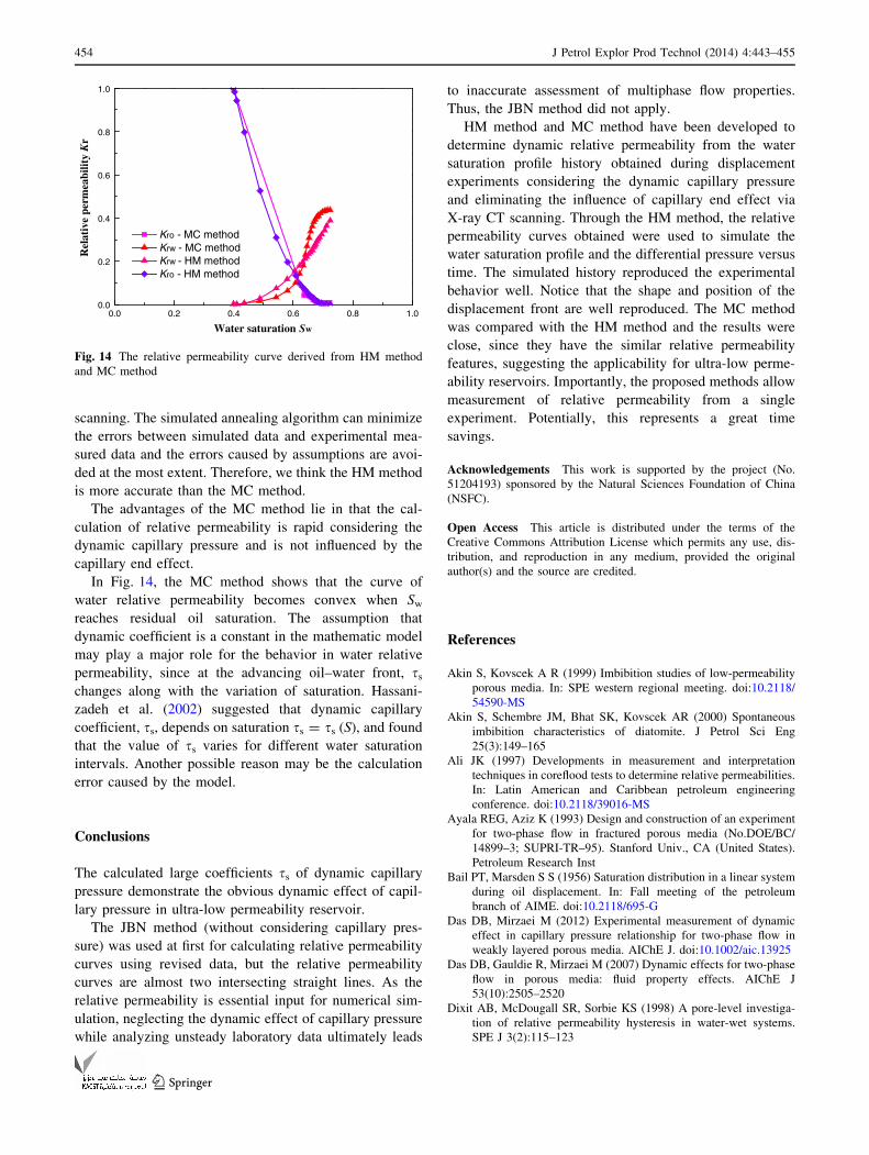
We validated the method embodied in Eqs. 26 and 34. The

relative permeability curves obtained, using Eqs. 26 and

34, were compared to the history matching curves in

Fig. 14. The curves obtained are close to the history

matching curves, with some scatter mainly related to the

representation of a laboratory-scale experiment, indicating

that both HM method and MC method can be applied in the

calculation of two-phase relative permeability for ultra-low

permeability reservoir. And the relative permeability

curves of both methods have some similar features, e.g.,

the common seepage area of oil–water two phases is very

narrow, the oil phase permeability decline rapidly, the

water phase permeability rising slowly at first then

increases rapidly.

However, we need also to see that the HM method is

more accurate than the MC method, since the mathematical

model is derived based on a series of assumptions. For the

MC method, there are errors caused by assumptions, such

as ignoring the pressure gradient of non-wetting phase and

ignoring the effect of capillary pressure and gravity in the

fractional flow equation, so that the influence of non-wet-

ting phase pressure gradient and capillary pressure on rel-

ative permeabilities cannot be reflected accurately. While

for the HM method, the water saturation profiles in

waterflooding process are measured through X-ray CT

0.0

0.2

0.4

0.6

0.8

1.0

Rel

ativ

e pe

rmea

bilit

y K

r

Water saturation Sw

Kro - MC methodKrw - MC method

0.0 0.2 0.4 0.6 0.8 1.0

Fig. 13 The relative permeability curve derived from mathematic

calculating method


123

scanning. The simulated annealing algorithm can minimize

the errors between simulated data and experimental mea-

sured data and the errors caused by assumptions are avoi-

ded at the most extent. Therefore, we think the HM method

is more accurate than the MC method.

The advantages of the MC method lie in that the cal-

culation of relative permeability is rapid considering the

dynamic capillary pressure and is not influenced by the

capillary end effect.

In Fig. 14, the MC method shows that the curve of

water relative permeability becomes convex when Sw

reaches residual oil saturation. The assumption that

dynamic coefficient is a constant in the mathematic model

may play a major role for the behavior in water relative

permeability, since at the advancing oil–water front, ss

changes along with the variation of saturation. Hassani-

zadeh et al. (2002) suggested that dynamic capillary

coefficient, ss, depends on saturation ss = ss (S), and found

that the value of ss varies for different water saturation

intervals. Another possible reason may be the calculation

error caused by the model.

Conclusions

The calculated large coefficients ss of dynamic capillary

pressure demonstrate the obvious dynamic effect of capil-

lary pressure in ultra-low permeability reservoir.

The JBN method (without considering capillary pres-

sure) was used at first for calculating relative permeability

curves using revised data, but the relative permeability

curves are almost two intersecting straight lines. As the

relative permeability is essential input for numerical sim-

ulation, neglecting the dynamic effect of capillary pressure

while analyzing unsteady laboratory data ultimately leads

to inaccurate assessment of multiphase flow properties.

Thus, the JBN method did not apply.

HM method and MC method have been developed to

determine dynamic relative permeability from the water

saturation profile history obtained during displacement

experiments considering the dynamic capillary pressure

and eliminating the influence of capillary end effect via

X-ray CT scanning. Through the HM method, the relative

permeability curves obtained were used to simulate the

water saturation profile and the differential pressure versus

time. The simulated history reproduced the experimental

behavior well. Notice that the shape and position of the

displacement front are well reproduced. The MC method

was compared with the HM method and the results were

close, since they have the similar relative permeability

features, suggesting the applicability for ultra-low perme-

ability reservoirs. Importantly, the proposed methods allow

measurement of relative permeability from a single

experiment. Potentially, this represents a great time

savings.

Acknowledgements This work is supported by the project (No.

51204193) sponsored by the Natural Sciences Foundation of China

(NSFC).

Open Access This article is distributed under the terms of the

Creative Commons Attribution License which permits any use, dis-

tribution, and reproduction in any medium, provided the original

author(s) and the source are credited.

References

Akin S, Kovscek A R (1999) Imbibition studies of low-permeability

porous media. In: SPE western regional meeting. doi:10.2118/

54590-MS

Akin S, Schembre JM, Bhat SK, Kovscek AR (2000) Spontaneous

imbibition characteristics of diatomite. J Petrol Sci Eng

25(3):149–165

Ali JK (1997) Developments in measurement and interpretation

techniques in coreflood tests to determine relative permeabilities.

In: Latin American and Caribbean petroleum engineering

conference. doi:10.2118/39016-MS

Ayala REG, Aziz K (1993) Design and construction of an experiment

for two-phase flow in fractured porous media (No.DOE/BC/

14899–3; SUPRI-TR–95). Stanford Univ., CA (United States).

Petroleum Research Inst

Bail PT, Marsden S S (1956) Saturation distribution in a linear system

during oil displacement. In: Fall meeting of the petroleum

branch of AIME. doi:10.2118/695-G

Das DB, Mirzaei M (2012) Experimental measurement of dynamic

effect in capillary pressure relationship for two-phase flow in

weakly layered porous media. AIChE J. doi:10.1002/aic.13925

Das DB, Gauldie R, Mirzaei M (2007) Dynamic effects for two-phase

flow in porous media: fluid property effects. AIChE J

53(10):2505–2520

Dixit AB, McDougall SR, Sorbie KS (1998) A pore-level investiga-

tion of relative permeability hysteresis in water-wet systems.

SPE J 3(2):115–123

0.0 0.2 0.4 0.6 0.8 1.00.0

0.2

0.4

0.6

0.8

1.0R

elat

ive

perm

eabi

lity K

r

Water saturation Sw

Kro - MC methodKrw - MC methodKrw - HM methodKro - HM method

Fig. 14 The relative permeability curve derived from HM method

and MC method


123

http://dx.doi.org/10.2118/54590-MS



http://dx.doi.org/10.2118/695-G

http://dx.doi.org/10.1002/aic.13925

Dixit A, Buckley J, McDougall S, Sorbie K (2000) Empirical

measures of wettability in porous media and the relationship

between them derived from pore-scale modelling. Transp Porous

Media 40(1):27–54

Donaldson EC, Dean GW (1966) Two- and three-phase relative

permeability studies. U.S.Bureau of Mines, Washington, DC

Fenwick DH, Blunt MJ (1998) Three-dimensional modeling of three

phase imbibition and drainage. Adv Water Resour 21(2):

121–143

Firoozabadi A, Aziz K (1988) Relative permeabilities from centrifuge

data. In: SPE California regional meeting. doi:10.2118/15059-

MS

Hassanizadeh SM, Gray WG (1990) Mechanics and thermodynamics

of multiphase flow in porous media including interphase

boundaries. Adv Water Resour 13(4):169–186

Hassanizadeh SM, Celia MA, Dahle HK (2002) Dynamic effect in the

capillary pressure-saturation relationship and its impacts on

unsaturated flow. Vadose Zone J 1(1):38–57

Hirasaki GJ, Rohan JA, Dudley JW (1995) Interpretation of oil/water

relative permeabilities from centrifuge displacement. SPE Adv

Technol Ser 3(1):66–75

Honarpour M, Mahmood SM (1988) Relative-permeability measure-

ments: an overview. J Petrol Technol 40(8):963–966

Hove AO, Ringen JK, Read PA (1987) Visualization of laboratory

corefloods with the aid of computerized tomography of X-rays.

SPE Reserv Eng 2(2):148–154

Huang DD, Honarpour MM (1998) Capillary end effects in coreflood

calculations. J Petrol Sci Eng 19(1):103–117

Hughes RG, Brigham WE, Castanier LM (1996) CT imaging of two

phase flow in fractured porous media. In: Proceedings of the 21st

workshop on geothermal reservoir, engineering. Stanford Uni-

versity, Stanford, pp 22–24

Janos T, Tibor B, Peter S, Faruk C (2001) Direct determination of

relative permeability from nonsteady-state constant pressure and

rate displacements. In: SPE production and operations sympo-

sium. doi:10.2118/67318-MS

Kamath J, de Zabala EF, Boyer RE (1995) Water/oil relative

permeability endpoints of intermediate-wet, low-permeability

rocks. SPE Form Eval 10(1):4–10

Kirkpatrick S, Gelatt CD, Vecchi MP (1983) Optimization by

simulated annealing. Science 220(4598):671–680

Lake LW (1989) Enhanced oil recovery, Chap. 3. Prentice Hall, Inc,

Englewood Cliffs

Lenormand R, Touboul E, Zarcone C (1988) Numerical models and

experiments on immiscible displacements in porous media.

J Fluid Mech 189(1):165–187

Lu W, Liu Q, Zhang Z et al (2012) Measurement of three-phase

relative permeabilities. Petrol Explor Dev 39(6):758–763

Mirzaei M, Das DB (2007) Dynamic effects in capillary pressure–

saturations relationships for two-phase flow in 3D porous media:

Implications of micro-heterogeneities. Chem Eng Sci 62(7):

1927–1947

Mitlin VS, Lawton BD, McLennan JD, Owen LB (1998) Improved

estimation of relative permeability from displacement experi-

ments. In: International petroleum conference and exhibition of

Mexico. doi:10.2118/39830-MS

Qadeer S, Dehghani K, Ogbe DO, Ostermann RD (1988) Correcting

oil/water relative permeability data for capillary end effect in

displacement experiments. In: SPE California regional meeting.

doi:10.2118/17423-MS

Stauffer F (1978) Time dependence of the relations between capillary

pressure, water content and conductivity during drainage of

porous media. In: IAHR symposium on scale effects in porous

media, vol 29. Thessaloniki, Greece. pp 335–352

The Oil and Gas Professional Standards Compilation Group of

People’s Republic of China (2007) SY/T 5345-2007 the test

method for relative permeability. Petroleum Industry Press,

Beijing

Topp GC, Klute A, Peters DB (1967) Comparison of water content-

pressure head data obtained by equilibrium, steady-state, and

unsteady-state methods. Soil Sci Soc Am J 31(3):312–314

Ucan S, Civan F, Evans R D (1993) Simulated annealing for relative

permeability and capillary pressure from unsteady-state non-

darcy displacement. In: SPE Annual technical conference and

exhibition. doi:10.2118/26670-MS

Vinegar HJ, Wellington SL (1987) Tomographic imaging of three-

phase flow experiments. Rev Sci Instrum 58(1):96–107

Wanna J (1982) Static and dynamic water content -pressure head

relations of porous media. Colorado State University, Fort

Collins

Wildenschild D, Hopmans JW, Simunek J (2001) Flow rate depen-

dence of soil hydraulic characteristics. Soil Sci Soc Am J

65(1):35–48

Withjack EM (1988) Computed tomography for rock-property

determination and fluid-flow visualization. SPE Form Eval

3(4):696–704


123







Documents

Determination of dynamic relative permeability in ultra