Determination of dimension of variety

& some applications

Author: Wenyuan Wu

 Supervisor: Greg Reid

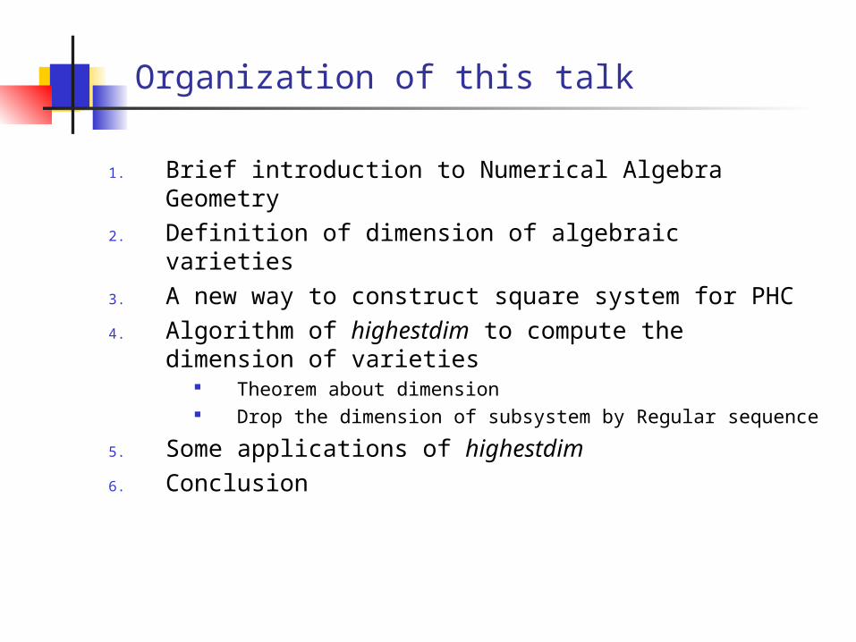
Organization of this talk

1. Brief introduction to Numerical Algebra Geometry2. Definition of dimension of algebraic varieties3. A new way to construct square system for PHC4. Algorithm of highestdim to compute the dimension of

varieties Theorem about dimension Drop the dimension of subsystem by Regular sequence

5. Some applications of highestdim 6. Conclusion

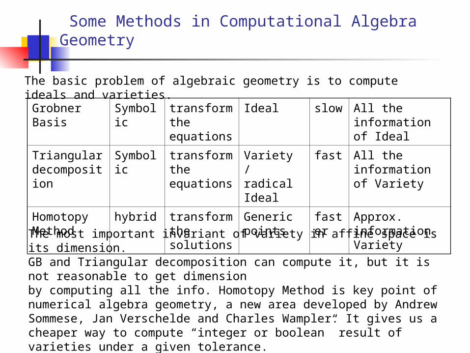
Some Methods in Computational Algebra Geometry

Grobner Basis Symbolic transform the equations

Ideal slow All the information of Ideal

Triangular decomposition

Symbolic transform the equations

Variety / radical Ideal

fast All the information of Variety

Homotopy Method

hybrid transform the solutions

Generic points

faster Approx. information Variety

The basic problem of algebraic geometry is to compute ideals and varieties.

The most important invariant of variety in affine space is its dimension. GB and Triangular decomposition can compute it, but it is not reasonable to get dimensionby computing all the info. Homotopy Method is key point of numerical algebra geometry, a new area developed by Andrew Sommese, Jan Verschelde and Charles Wampler. It gives us a cheaper way to compute “integer or boolean” result of varieties under a given tolerance.

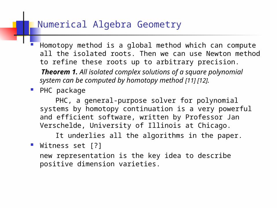
Numerical Algebra Geometry Homotopy method is a global method which can compute all the

isolated roots. Then we can use Newton method to refine these roots up to arbitrary precision.

Theorem 1. All isolated complex solutions of a square polynomial system can be computed by homotopy method [11] [12].

PHC package

PHC, a general-purpose solver for polynomial systems by homotopy continuation is a very powerful and efficient software, written by Professor Jan Verschelde, University of Illinois at Chicago.

It underlies all the algorithms in the paper. Witness set [?]

new representation is the key idea to describe positive dimension varieties.

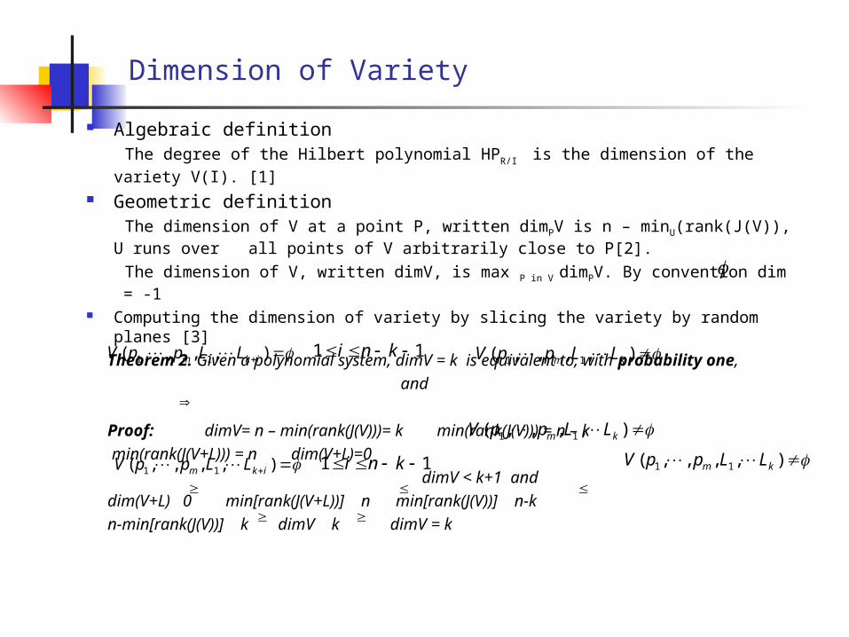
Dimension of Variety

Algebraic definition The degree of the Hilbert polynomial HPR/I is the dimension of the variety V(I).

[1] Geometric definition

The dimension of V at a point P, written dimPV is n – minU(rank(J(V)), U runs over all points of V arbitrarily close to P[2].

The dimension of V, written dimV, is max P in V dimPV. By convention dim = -1 Computing the dimension of variety by slicing the variety by random planes

[3] Theorem 2. Given a polynomial system, dimV = k is equivalent to, with probability one,

and

Proof: dimV= n – min(rank(J(V)))= k min(rank(J(V))) = n – k

min(rank(J(V+L))) = n dim(V+L)=0

dimV < k+1 and

dim(V+L) 0 min[rank(J(V+L))] n min[rank(J(V))] n-k

n-min[rank(J(V))] k dimV k dimV = k

),,,,( 11 ikm LLppV 11 kni ),,,,( 11 km LLppV

),,,,( 11 km LLppV

),,,,( 11 ikm LLppV 11 kni ),,,,( 11 km LLppV

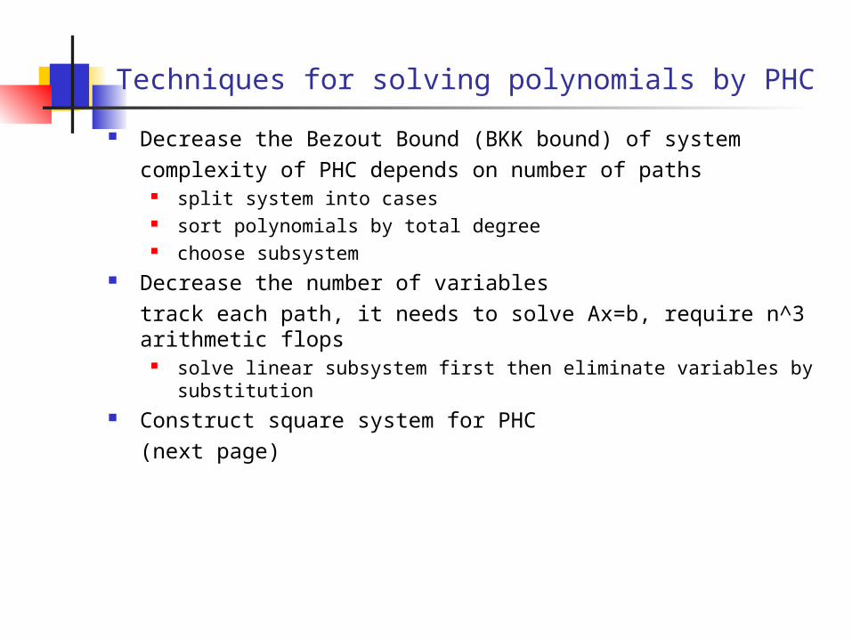
Techniques for solving polynomials by PHC

Decrease the Bezout Bound (BKK bound) of system

complexity of PHC depends on number of paths split system into cases sort polynomials by total degree choose subsystem

Decrease the number of variables

track each path, it needs to solve Ax=b, require n^3 arithmetic flops solve linear subsystem first then eliminate variables by substitution

Construct square system for PHC

(next page)

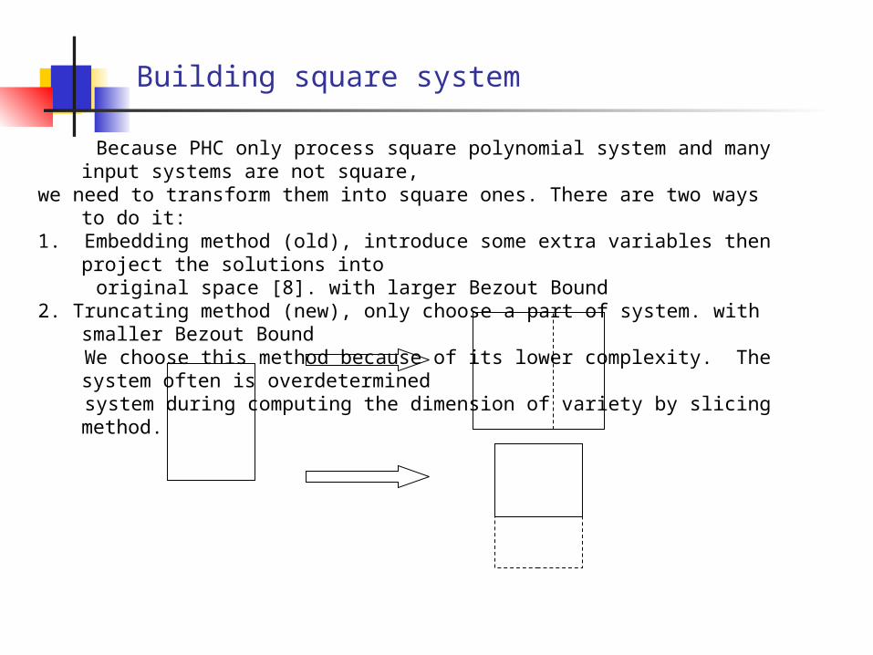
Building square system Because PHC only process square polynomial system and many input systems are not square,we need to transform them into square ones. There are two ways to do it:1. Embedding method (old), introduce some extra variables then project the solutions into original space [8]. with larger Bezout Bound2. Truncating method (new), only choose a part of system. with smaller Bezout Bound We choose this method because of its lower complexity. The system often is overdetermined system during computing the dimension of variety by slicing method.

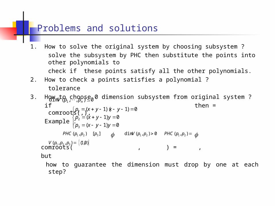
Problems and solutions

1. How to solve the original system by choosing subsystem ?

solve the subsystem by PHC then substitute the points into other polynomials to

check if these points satisfy all the other polynomials.

2. How to check a points satisfies a polynomial ?

tolerance

3. How to choose 0 dimension subsystem from original system ?

if then = comroots(,),

Example :

comroots( , ) = ,

but

how to guarantee the dimension must drop by one at each step?

0),,(dim 1 nppV

0)1(

0)1(

0)1)(1(

3

2

1

yyxp

yyxp

yxyxp

0),(dim 21 ppV ),( 21 ppPHC ),( 21 ppPHC ][ 3p ),,( 321 pppV )0,1(

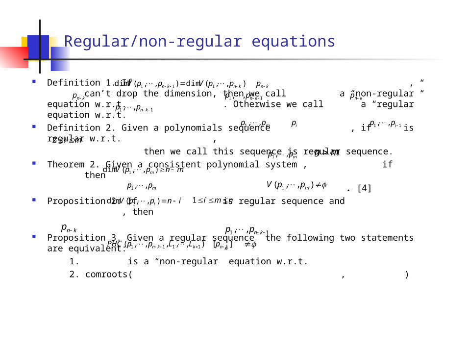
Regular/non-regular equations Definition 1. If , can’t drop the dimension, then we

call a “non-regular” equation w.r.t. . Otherwise we call a “regular” equation w.r.t.

Definition 2. Given a polynomials sequence , if is regular w.r.t. ,

then we call this sequence is regular sequence. Theorem 2. Given a consistent polynomial system , if then

. [4] Proposition 2. If is regular sequence and , then

Proposition 3. Given a regular sequence the following two statements are equivalent:

1. is a “non-regular” equation w.r.t.

2. comroots( , )

),,(dim),,(dim 111 knkn ppVppV knp

knp 11 ,, knpp knp

11 ,, knpp

mpp ,,1 ip 11 ,, ipp

mi 2

mpp ,,1 mn

mnppV m ),,(dim 1

mpp ,,1 ),,( 1 mppV

inppV i ),,(dim 1 nmi 1

knp 11 ,, knpp

),,,,,( 1111 kkn LLppPHC ][ knp

How to build the regular sequence

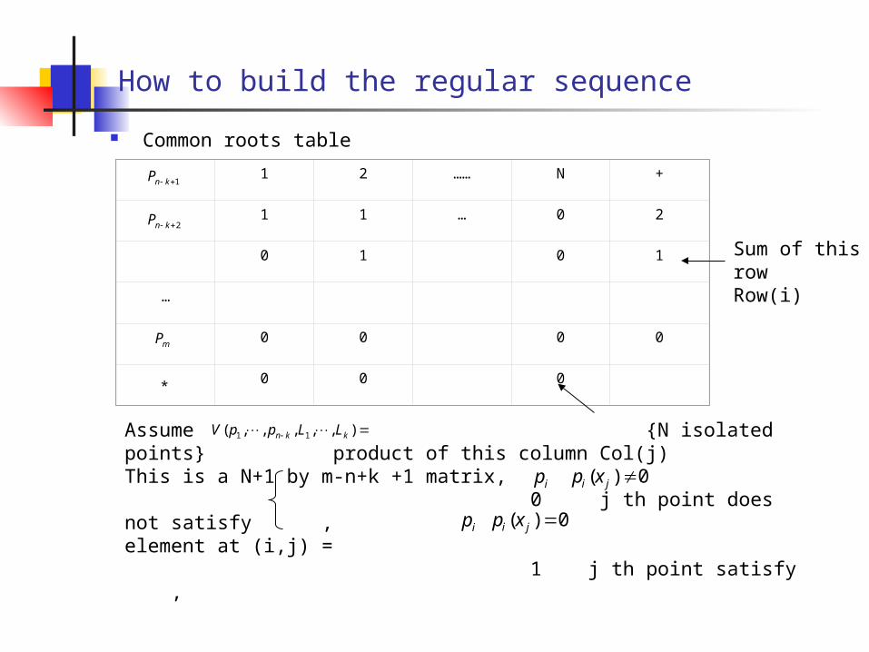
Common roots table

1 knP

2 knP

mP

  1 2 …… N +

1 1 … 0 2

0 1   0 1

…          

0 0   0 0

0 0   0  

Assume {N isolated points} product of this column Col(j)This is a N+1 by m-n+k +1 matrix, 0 j th point does not satisfy ,element at (i,j) = 1 j th point satisfy ,

),,,,,( 11 kkn LLppV

*

0)( ji xpip

ip 0)( ji xp

Sum of this rowRow(i)

continue

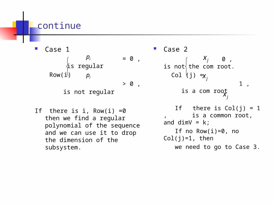
Case 1 = 0 , is regular

Row(i)

> 0 , is not regular

If there is i, Row(i) =0 then we find a

regular polynomial of the sequence and we can use it to drop the dimension of the subsystem.

Case 2 0 , is not the com root.

Col (j) =

1 , is a com root

If there is Col(j) = 1 , is a common root, and dimV = k;

If no Row(i)=0, no Col(j)=1, then

we need to go to Case 3.

ip

ip

jx

jx

jx

continue

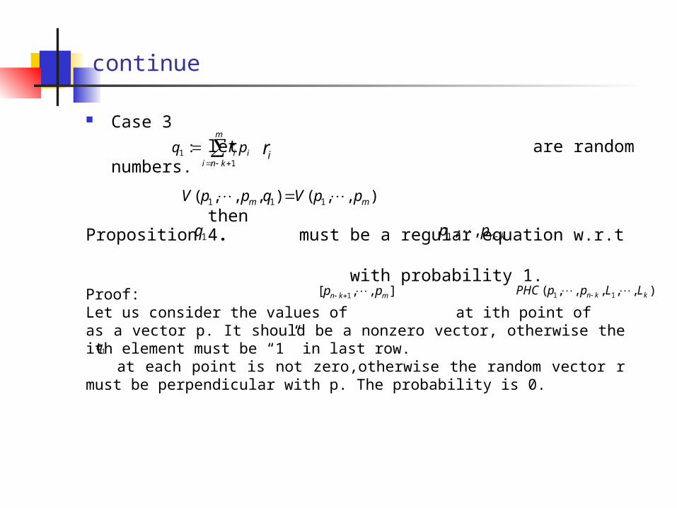
Case 3

let are random numbers.

then

m

kniii prq

11 :

ir

),,(),,,( 111 mm ppVqppV

Proposition 4. must be a regular equation w.r.t with probability 1. Proof: Let us consider the values of at ith point of as a vector p. It should be a nonzero vector, otherwise the ith element must be “1” in last row. at each point is not zero,otherwise the random vector r must be perpendicular with p. The probability is 0.

1q knpp ,,1

],,[ 1 mkn pp ),,,,,( 11 kkn LLppPHC

1q

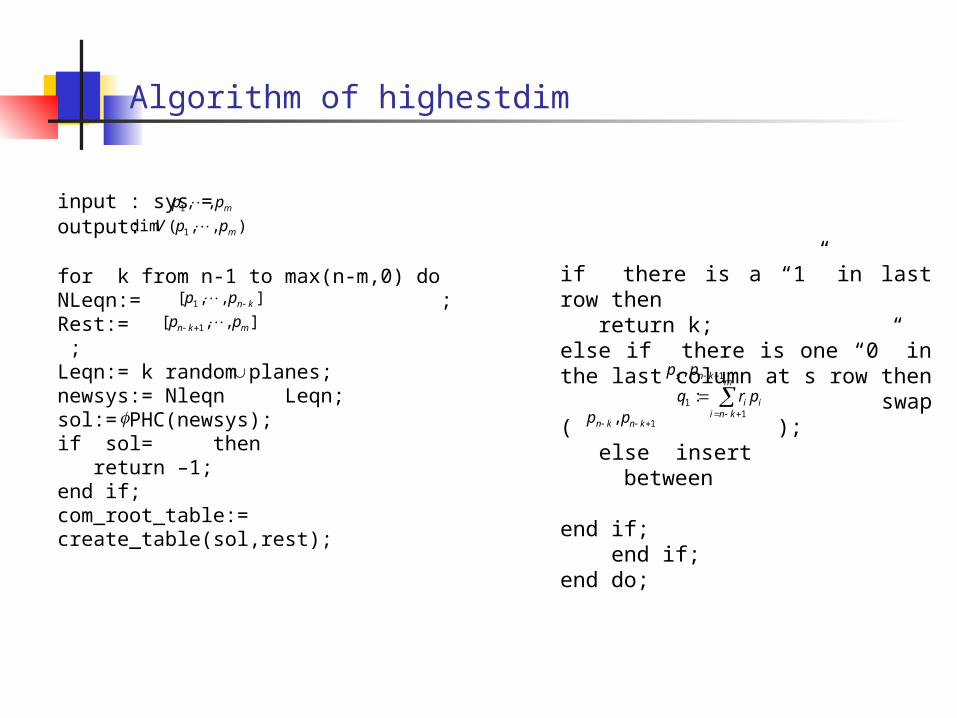
Algorithm of highestdim

input : sys = output:

for k from n-1 to max(n-m,0) doNLeqn:= ;Rest:= ;Leqn:= k random planes;newsys:= Nleqn Leqn;sol:= PHC(newsys);if sol= then return –1;end if;com_root_table:= create_table(sol,rest);

mpp ,,1 ),,(dim 1 mppV

if there is a “1” in last row then return k;else if there is one “0” in the last column at s row then swap ( ); else insert between end if; end if;end do;

],,[ 1 knpp ],,[ 1 mkn pp

1, kns pp

m

kniii prq

11 :

1, knkn pp

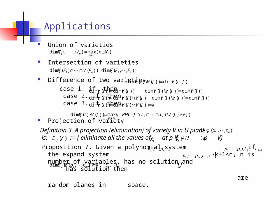
Applications

Union of varieties Intersection of varieties Difference of two varieties case 1. if then case 2. if then case 3. if then

Projection of variety

Proposition 7. Given a polynomial system , if the expand system , k+1<n, n is number of variables, has no solution and has solution then

are random planes in space.

)(dimmax)dim(1

1 ini

n VVV

)),,(dim())()(dim( 11 nn FFVFVFV

)):(dim())(\)(dim( JIVJVIV

))(dim())(dim( JVIV ))(dim())(\)(dim( IVJVIV ))()(dim())(dim( JVIVIV

))(dim())(\)(dim( IVJVIV

kJVIVIV ))()(dim())(dim(

}))(\)(:{max))(\)(dim( 10

JVLLIPHCiJVIV iki

Definition 3. A projection (elimination) of variety V in U plane , is: := { eliminate all the values of at p if : p V}

},,{ 1 nxxU

)(VEU ix Uxi

mpp ,,1 111 ,,,, km LLpp

km LLpp ,,,, 11

kppVE mU )),,((dim 1 kLL ,1 U

continue

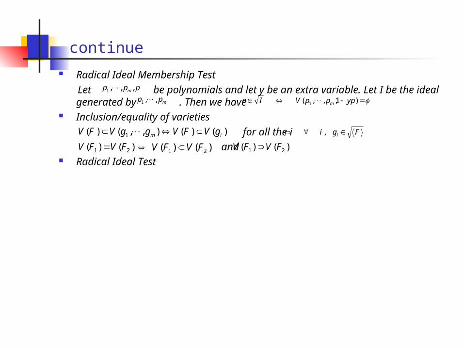
Radical Ideal Membership Test

Let be polynomials and let y be an extra variable. Let I be the ideal generated by . Then we have

Inclusion/equality of varieties

for all the i

and Radical Ideal Test

ppp m ,,,1

mpp ,,1 )1,,,( 1 ypppVIp m

)()(),,()( 1 im gVFVggVFV Fgi i ,

)()( 21 FVFV )()( 21 FVFV )()( 21 FVFV

Conclusion

a new numerical symbolic method “highestdim” which has lower complexity to determine the dimension of variety

a new way to test radical ideal membership based on “highestdim” Application in RIF package of Maple

Reference

[2] David Cox, John Little and Donal O’Shea. Using Algebra Geomery. Springer-Verlag, (1998) New York.

[4] David Cox, John Little and Donal O’Shea. Ideals, Varieties, and Algorithms. Springer-Verlag, (1997) New York.

[8] Andrew J. Sommese and Jan Verschelde: Numerical Homotopies to compute Generic Points on Positive Dimensional Algebraic Sets. The Abstract and gzipped postscript file, Revised version. Journal of Complexity 16(3):572-602, 2000.

[11] GARCIA, C. B. and ZANGWILL, W. I., "Finding all solutions to polynomial systems and other systems of equations," Math. Program. 16, pp. 159-176 (1979).

[12] T.Y. Li and X. Wang. Nonlinear homotopies for solving deficient polynomial systems with parameters. SIAM J. Numer. Anal., 29(4):1104-1118, 1992.

Keith Kendig, Elementary Algebraic Geometry. Springer-Verlag, (1997) New York.